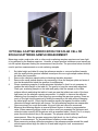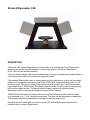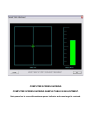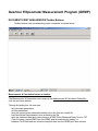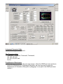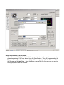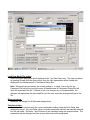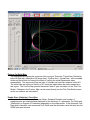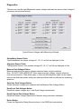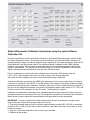
1
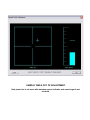
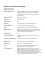
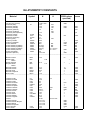
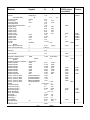
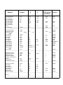
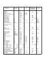
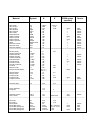
LSE STOKES ELLIPSOMETER USER MANUAL 7109-C370B GAERTNER SCIENTIFIC CORPORATION 3650 W. Jarvis Ave., Skokie, IL 60076 USA TEL: 847 673 5006; FAX: 847 673 5009 www.GaertnerScientific.com OPTIONAL SCATTER MODIFICATION FOR SOLAR CELL OR ROUGH SCATTERING SAMPLE MEASUREMENT Measuring certain rough solar cells or other rough scattering samples requires more laser light to be gathered by the analyzer aperture. However, a larger aperture introduces more inaccuracy into the optical alignment making the measurement less precise. The procedure below should be used to perform measurements on such scattering samples. 1. 2. 3. 4. 5. 6. Set table height and table tilt using the reference sample or a normal polished sample with the small pinhole aperture installed in analyzer since a rough sample makes setting the table often impossible. Remove the reference sample without disturbing the table alignment. Remove the small pinhole aperture by unscrewing it from the analyzer plate and screw it into the threaded hole below the aperture for safekeeping. Chose a scattering sample of similar substrate thickness so that it is not necessary to readjust the table height or the table tilt. The goal is to keep the same table alignment. Place your scattering sample on the table and gently slide the sample on the table surface without readjusting the table to locate an area that reflects as much of the laser light beam into the analyzer opening as possible. It is helpful to observe the reflected scattering from the sample on the large ring surrounding the aperture opening. Direct as much of the light into the aperture by sliding the sample on the table without changing the table height and tilt. Check that the sample remains flat against the table surface otherwise the angle and height will change. Not all scattering samples are measurable. Some are simply too rough and scatter too much light and cannot be measured. Measure the scattering sample at several different regions to obtain a representative value. When measuring silicon nitride on silicon enter your expected film thickness and refractive index normally 800 Angstroms with an expected index 2.0 and 0 for K or simply press the nitride shortcut key in the program. The program should make the measurement. When the program encounters light levels too low it will say insufficient power for measurement. Try several different locations on the sample. When measuring ordinary reflective samples or the reference sample reinstall the small pinhole aperture and align the table for tilt and table height for best measurement accuracy. LASER SAFETY CERTIFICATION All laser Ellipsometers supplied by Gaertner comply with CDRH requirements 21CFR 1040 for a class II laser product emitting less than 1 milliwatt or class llla (less than 5 milliwatt) of low power radiation. As with any bright source such as the sun or arc lamp, the operator should not stare directly into the laser beam or its reflection from highly reflecting surfaces. Appropriate Warning Logotypes and Aperture labels alert users and service personnel of the presence of laser radiation during operation. Reproductions of these labels are shown. WARRANTY All optical, mechanical and electrical components of Gaertner Ellipsometers, including the lasers are warranted for one year from the date of delivery. Gaertner will correct any defects in material or workmanship at no cost. Shipping charges, travel and lodging costs incurred by service personnel are not covered by this warranty. Warranty on defects in material and workmanship for any computer, computer monitor and printer supplied with the Ellipsometer is covered by its respective manufacturer and is passed through onto the user. The computer manufacturer will, at their option, repair or replace equipment that proves defective during the warranty period. Repairs necessitated by the misuse of the equipment, including use of software or interfacing not supplied by Gaertner, are not covered by this warranty. No other warranty is expressed or implied, including, but not limited to, implied warranty of merchantability and suitability for a particular purpose. Gaertner shall not be liable for consequential damages. OPERATING INSTRUCTIONS DO NOT turn on the power supply WITHOUT A LASER CONNECTED. If you do turn off the power supply and wait AT LEAST FIVE MINUTES before connecting the laser. 1. 2. 3. 4. Make certain the power switch (front panel) is in the “0” (OFF) position. Check that the voltage setting on the voltage selector switch (REAR PANEL) matches the input voltage. Insert the line cord into the receptacle (REAR PANEL). Plug the other end of the line cord into an appropriate receptacle. Plug the male high voltage connector from the laser head into the high voltage receptacle (REAR PANEL). This connection is a TIGHT FIT. To prevent faulty operation, be sure the male connector is FULLY SEATED. To prevent the possibility of electric shock, FULLY TIGHTEN THE HIGH VOLTAGE CONNECTOR RETAINING SCREW (under high voltage receptacle). Turn the power supply on by switching the power switch to “1” (ON). The INDICATOR LIGHT will turn on IMMEDIATELY. There will be a THREE TO SEVEN SECOND SAFETY DELAY before the laser turns on. On lasers equipped with a safety shutter, laser emission WILL NOT BE VISIBLE UNTIL THE SHUTTER IS OPENED. REMOTE CONNECTOR WARNING-PREVENTION OF ELECTRIC SHOCK: To maintain the conformance of this unit with the requirements of EN61010 - 1:1993, the power supply must be SWITCHED OFF AND DISCONNECTED FROM MAINS POWER before removing the remote plug from the socket. The remote connector is provided as a safety feature to allow REMOTE ACTUATION of the laser power supply if remote actuation is desired, ensure that the cable and remote switch are RATED FOR THE SPECIFIED POWER SUPPLY INPUT VOLTAGE AND CURRENT. The remote switch WILL ACTUATE THE POWER SUPPLY ONLY WHEN THE MAIN POWER SWITCH IS SWITCHED ON. As supplied, the polarized remote connector plug is WIRED WITH AN INTERNAL JUMPER. If the connector is to be used with a remote external switch, modify the plug as follows: 1. 2. 3. 4. 5. 6. 7. 8. 9. Switch OFF power and disconnect power supply from mains power. Remove remote connector plug from its socket (REAR PANEL) by pulling straight out. Press out the silver-colored locking pin. Remove plug shell. Remove the shorting wire from the plug terminals. Drill or punch a hole in the flat end of the plug shell. Slide the plug shell onto the remote connector cable. Solder the cable leads to the plug terminals. Insert the connector into its receptacle. FUSING 1. 2. The power supply is protected by an INTERNAL, NON-REPLACEABLE FUSE. The fuse is rated 230 VOLTS, 1 ½ AMP, NORMAL ACTING. IF YOU EXPERIENCE A PROBLEM… CHECK: 1. 2. 3. 4. 5. 6. That the indicator light is on, indicating presence of line voltage. That the laser shutter is open, if provided. That the remote plug is firmly inserted in the remote connector receptacle. That the remote switch is switched on, if used. That the high voltage connector is firmly inserted in the high voltage receptacle. That the voltage selector switch is set correctly. If the power supply is not operated in accordance with these instructions, the function of essential safety features may be impaired. The laser power supply has no user serviceable parts within and requires no user maintenance. Top Module Contains Alignment Laser Diode and Position Sensor Entrance Aperture on Inside Plate Sample Table Left Module Contains Measuring Laser Right Module Contains StokesMeter™ Detector & Interface to PC Base Plate LSE STOKES Ellipsometer INSTALLATION INSPECTION Inspect the shipping container and the Ellipsometer for shipping damage. Verify that the Sample Table, Sample Wafer, Computer Interface Card, Laser Power Supply and User Manual with CD’s software disks are removed from the shipping container together with the Ellipsometer. LOCATION CONSIDERATIONS The LSE Ellipsometer is designed for use in either a production or laboratory facility under environmentally controlled conditions providing relatively constant room ambient temperature at 20ºC (68ºF) and dry, dust-free atmosphere. The Ellipsometer requires a clean, solid, level work surface. The LSE Ellipsometer alignment laser and StokesMeter™ detector is powered by the computer interface card that in turn is powered by the computer. The HeNe measuring laser is powered by its own separate key operated powered supply. The line voltage to the equipment should be free of transients having harmonies in the range from audio frequencies to several megahertz. A voltage surge protector is recommended for the system power. INSTALLATION Install the National Instruments NI-DAQmx Software Driver and reboot the computer before connecting the USB cable between the Ellipsometer and the computer. 1. Install the NI-DAQmx Software Driver on your WINDOWS 8/7/VISTA/ XP computer using the supplied DVD or download the NI-DAQmx Driver from the NI.COM website. Allow the computer to reboot to complete installation. It is not necessary to install documentation. Allow configuration of the NI-DAQmx Measurement and Automation Explorer. 2. Connect the USB cable to the ellipsometer interface located on the bottom of the right hand module and to a USB connection on your PC using the supplied USB cable. This connection also powers the ellipsometer laser diode used for sample alignment. 3. Upon booting up the computer, the USB Interface should be automatically recognized by the computer. To verify this, run the NI Measurement and Automation Explorer from the icon on your desktop. View Devices and Interfaces and the NI USB 6211 interface should be shown. 4. Run SETUP from the CD to install the Gaertner GEMP Software. The GEMP program will be loaded into the C: \ GSC directory. 5. Run C: \ GSC \ GEMP.exe program to make measurements. Check operation by measuring the reference sample. If the following WINDOWS error is encountered: 1. Setup.exe - Entry Point Not Found The procedure entry point HeapSetInformation cound not be located in the dynamic link library KERNEL32.dll Install the appropriate Windows Hotfix contained within the directory \KB835732\Win2000 or WinXP found in the GSC directory 2. If you get the following message when trying to start the GEMP program, C:\GSC\GEMP.exe This application has failed to start because the application configuration is incorrect. Reinstalling the application may fix this problem. Run the Windows redistributable vcredist_x86.exe found in the GSC directory. Should the installation fail recheck the steps above. If communication still fails try another computer. Stokes Ellipsometer LSE DESCRIPTION The model LSE Stokes Ellipsometer is a continuation of an entirely new line of Ellipsometer based on the revolutionary StokesMeter™ technology (winner of Photonics Spectra and R & D 100 best new products awards). The unit’s elegant design offers unprecedented ease of use and instantaneous measurement at a cost much lower than conventional metrology instruments. This patented Ellipsometer uses no moving parts and no modulators to quickly and accurately determine the complete polarization state of the 6328Å HeNe Laser measuring beam at a 70º incidence angle. The space-saving design features a small footprint yet it can accommodate large samples up to 300mm wide. The sample stage is rapidly moved by hand to measure any point on the sample surface. The sample table includes a manual tilt and table height adjustment, which is set using an alignment screen on the computer. GEMP Windows Software can measure the top layer film thickness and film refractive index on a substrate or on 1, 2 or 3 known bottom layers. The films can be transparent or absorbing. This durable integration of hardware and software is fast and easy to use. Extremely precise, stable and low cost the model LSE Stokes Ellipsometer represents an excellent value in a basic Ellipsometer. DESCRIPTION OF TECHNOLOGY This patented device uses no moving parts and no modulators to quickly and accurately determine the complete polarization state of the measuring beam. ABSTRACT A photopolarimeter meter for the simultaneous measurement of all four Stokes parameters of light. The light beam, the state of polarization of which is to be determined, strikes, at oblique angles of incidence, three photodetector surfaces in succession, each of which is partially spectrally reflecting and each of which generates an electrical signal proportional to the fraction of the radiation it absorbs. A fourth photodetector is substantially totally light absorptive and detects the remainder of the light. The four outputs thus developed form a 4 x 1 signal vector I which is linearly related, I = AS, to the input Stokes vector S. Consequently, S is obtained by S = A (-1) I. The 4 x 4 instrument matrix A must be nonsingular, which requires that the planes of incidence for the first three detector surfaces are all different. For a given arrangement of four detectors, A can either be computer or determined by calibration. The clean, compact StokesMeter™ replaces a typical rotating Analyzer Assembly consisting of a Drum, Prism, Encoders, Switches, Motor and Detector and their associated electronics. In addition, the waveplate mechanism on the Polarizer Arm is eliminated. This result in a fact, precise, stable no moving parts Ellipsometer. StokesMeter™ References R.M.A. Azzam and N.M. Bashara, Ellipsometery and Polarized Light (North-Holland, Amsterdam, 1987). M.Bom and E.Wolf, Principles of Optics (Pergamon, New York, 1975). W.A. Shurcliff, Polarized Light (Harvard Univ. Press Cambridge, MA, 1962). R.M.A. Azzam, “ Measurement of the Stokes parameters of light; A unified analysis of Fourier photopolarimetry” Optik 52, 253-256 (1979). R.M.A. Azzam, “ Division-of-amplitude photopolarimeter (DOAP) for the simultaneous measurement of all four Stokes parameters of light”, Optica Acta 29, 685-689 (1982). R.M.A. Azzam, “Beam splitters for the division-of-amplitude photopolarimeter (DOAP)”, Optica Acta 32, 1407-1412 (1985). R.M.A. Azzam, “Arrangement of four photodetectors for measuring the state of polarization of light”, Opt. Lett 10, 309-311 (1985). U.S. Patent 4,681,450 (July 21, 1987). R.M.A. Azzam, E. Masetti, I.M. Elminyawi and F.G. Grosz, “Construction, calibration, and testing of a four-detector photopolarimeter”, Rev. Sci. Instrum. 59, 84-88 (1988). R.M.A. Azzam, I.M. Elminyawi and A.M. El-Saba, “General analysis and optimization of the fourdetector photopolarimeter”, J. Opt. Soc. Am. A 5, 681-689 (1988). R.M.A. Azzam and A.G. Lopez, “Accurate calibration of the four-detector photopolarimeter with imperfect polarizating optical elements”, J. Opt. Soc. Am. A 6, 1513-1521 (1989). R.M.A. Azzam, “Instrument matrix of the four-detector photopolarimeter: Physical meaning of its rows and columns and constraints on its elements”, J. Opt. Soc. Am. A 7, 87-91 (1990). R.M.A. Azzam and A.G. Lopez, “Precision analysis and low-light-level measurements using a prototype four-detector photopolarimeter”, Rev. Sci. Instrum. 61, 2063-2068 (1990). M.R. Latta and S.L. Heesacker, “Measurement of polarization components using a four-detector polarimeter”, SPIE Proc. 1166, 207-219 (1990). R.M.A. Azzam, K.A. Giardina and A.G. Lopez, “Conventional and generalized Mueller-matrix ellipsometry using the four-detector photopolarimeter “, Opt. Eng. 30, 1583-1589 (1991). MEASUREMENT The model LSE STOKES ELLIPSOMETER is constructed using optical and solid state components and contains no mechanical moving parts (apart from the sample table). This insures highly reliable measurements and long-term stability. The LSE uses two low power lasers (less than 5 milliwatt) for sample measurement and alignment. The HeNe 632.8 nm measurement beam, after reflecting from the sample, enters a patented arrangement of 4 stationary photodiode detectors that instantaneously determine the polarization state of the reflected measuring beam. A separate solid-state alignment laser beam at 670 nm strikes the sample at normal incidence sending the beam to a position sensor permitting the sample tilt and height to be adjusted via an alignment screen on the computer (see following diagrams). Laser Safety Prior to turning on the ellipsometer please refer to the diagram noting the location of the laser beam exit apertures and the entrance aperture. The measuring beam exit aperture is located on the left module inside plate and the alignment aperture is on the top inside plate. Although the design of the instrument makes direct laser contact with the eyes unlikely; the use of low power lasers under 5mW (less than the power output found in some laser pointers) further adds to the safety of the instrument. Regardless: Please observe laser caution to prevent any possible eye damage from looking into the laser beam or its specular reflection. Sample Measurement Familiarize yourself with the sample table. Operate the two sample table tilt knobs and the table height adjustment with the table removed from the ellipsometer. Freely manipulate the table adjustments until these adjustments are understood and easily performed. The table adjustment is the only subjective user adjustment directly affecting the accuracy of the measurements. 1. Place the sample table over the screw at the center of the base plate and secure the table base using the thumb screw from underneath the base plate if desired. 2. For laser safety, verify that the laser shutter plate ( located on the top module) is blocking the exit aperature. The separate HeNe laser power supply should not be turned on without first connecting it to the HeNe laser (Refer to the OPERATING INSTRUCTIONS described earlier). 3. With the interface card, cable and software installed (refer to installation instructions) turn the computer on. The computer interface card supplies power to the alignment laser located in the top module and the StokesMeter detector located in the right module.. Alignment laser emission is controlled by your computer. With the interface cable connected the alignment laser is on when the computer is turned on. A mechanical shutter plate is located at the exit aperature of the alignment laser located in the top module. Check that the mechanical shutter plate is now fully open. The laser alignment beam should now be visible if you wave your hand over the sample table 4. The measurement point is indicated by the alignment laser beam spot on the table surface. This beam location will be difficult to see on very clean samples so keep the table position as a reference. Do not turn on the separate HeNe power supply without first connecting the male high voltage connector from the left laser module into the high voltage receptacle of the separate power supply. With the HeNe laser connected, turn the power supply on. Open the mechanical laser shutter located at the HeNe laser exit aperture by rotating the knurled wheel in a downward direction. The reflected beam should be visible against the inside plate on the right side. 5. Place a sample on the table. The sample may be centered using the table rings as a reference. The table itself can be centered with respect to the instrument by observing the alignment laser beam position on the table surface with the sample removed. 6. Run the GEMP measurement program. Refer to the pages that follow for a detailed explanation of this program. 7. Enter the Measurement and Calculation window by clicking on the ellipsometer icon on the GEMP program toolbar. 8. Prior to any measurement, the sample table must be adjusted. Clicking on the Sample Alignment button with your mouse to enter the alignment screen. First adjust the tilt by working the sample table tilt knobs until the target cross is centered on the screen (see diagram). Note that tilt should always be adjusted first. Second adjust the height by working the sample table vertical adjustment wheel to obtain maximum power to the detector. This occurs when the longer horizontal bar reaches and is even with the shorter index bar. The shorter index bar indicates the maximum power that has been obtained thus far, while the longer index bar indicates the actual power that is currently entering the aperture. Raise and lower the sample table through the maximum to mark the maximum power position. For a preliminary table height alignment, observe the location of the laser beam at the 1 mm entrance aperture located on the right module inner plate and adjust the sample table height until the measurement laser beam enters the aperture. 9. Return to the GEMP program Measurement and Calculation window. Execute the measurement by clicking the Measure and Calculate button or one of the Shortcut buttons (e.g. Thin Oxide, Thin Nitride). See the GEMP Calculation Mode on the pages that follow for further information. SAMPLE TABLE Adjustment of the sample table is done with the aid of the GEMP program by clicking on the Sample Table Adjustment button. A sample table power bar and cross target tilt adjustment screen are displayed on the computer monitor. Place the wafer on the table. The table rings serve as a useful reference to help center the wafer. For a preliminary “ballpark” alignment observe the laser beam reflection at the 1 mm entrance aperture located on the right module inner plate. Adjust the table tilt and height until the beam enters the aperture. USE ONE HAND TO HOLD STEADY THE TABLE BASE (if not secured to the base plate with the fastening screw) AND WITH THE OTHER HAND WORK THE TABLE ADJUSTMENTS. First adjust the sample tilt by turning the tilt adjustment x and y plane knobs under the table until the target cross is centered within the TILT screen. The tilt is always adjusted first. Next adjust the table height by turning the vertical adjustment wheel to raise the power bar and the shorter index bar to their highest position. The maximum position is marked by the shorter index bar when the table passes thru the maximum power position. The table height is correct when the power bar is approximately even with the shorter index bar. SAMPLE TABLE OUT OF ADJUSTMENT. Note power bar is not even with maximum power indicator and cross target is not centered. COMPUTER SCREEN SHOWING COMPUTER SCREEN SHOWING SAMPLE TABLE IN ADJUSTMENT. Note power bar is even with maximum power indicator and cross target is centered. Gaertner Ellipsometer Measurement Program (GEMP) DOCUMENT PRINT AREA WINDOW Toolbar Buttons Toolbar buttons have corresponding menu commands as shown below. Measurement & Calculation button on toolbar. The Measurement & Calculation button pops up the Measurement & Calculation Dialog Box over the print area window. Through this dialog box, the user can: set instrument parameters, set film parameters, save the current active parameters setting into a tfm (thin film model) file, load New Model file parameters from an existing tfm file, save the measured data and current setup to a SMD (Store Measured Data) file or a TXT (Text) file open a saved SMD file to the GEMP print area window by loading, or measure Psi & Delta and two solutions and print them into the GEMP print area window. Instrument Parameter fields: Phi, Wavelength and Ambient N Film Parameter fields: Thickness1, Thickness2, Thickness3, Thickness4, Nf1, Nf2, Nf3, Nf4, Kf1, Kf2, Kf3, Kf4, and Ns, Ks Print Measured Data button: Prints the measured data to the print area window. (Since the GEMP print area window is behind the Measurement & Calculation Dialog Box, the user may need to move the Measurement & Calculation Dialog Box by dragging it to see part of the GEMP print area window.) Save Current Model to a file button: Opens the Save As dialog box in which the user can type in the file name to save current parameters setting. If the user doesn’t type the file extension, *.tfm will be appended to the file name the user has typed in. For example, if the user typed test1 in the File name: field, the file name will be test1.tfm . Since this file is a normal text file, the user can use any text editing program to see the contents. Load New Model File button: Opens the Open dialog box which displays all the *.tfm files if there are. The user can select an existing file and click the Open button, then the file’s parameters will be loaded and displayed in the Measurement & Calculation Dialog Box. Note: Whenever the user saves, the current setting to, or loads, from a tfm file, the Parameter File field at the top-right corner of Measurement & Calculation Dialog Box will show the associated tfm file. However, if the user changes any of the parameters, the changes will not update the associated file until the user saves the changed settings to the file. Measure button: Measures the sample Psi & Delta and displays them. Calculate button: Calculates the 2 solutions with the current parameters setting using the Psi & Delta and displays the result. Psi, and Delta values or model parameters can also be manually entered into the edit fields. Solutions 1 and Solutions 2 are calculated using the entered values. The parameters can be changed as often as you wish and results recalculated. Measure and Calculate button: Measures and displays the Psi and Delta and does the calculation in the selected Calculation Mode with entered parameter values and displays the result. If the Automatic Print Data field is checked, the Psi & Delta, and the calculation result will print into the GEMP print area window. Calculation Modes or Combinations: The GEMP software acquires data from the ellipsometer and calculates the ellipsometer values of Psi and Del for the measured sample. The calculation modes in the software offer various choices for converting the results of the Psi & Del measurement into a user-constructed model of the sample. Enter values of film thickness, film refractive index Nf and absorption Kf into the sample model fields. Simply click 2 of the desired parameters to be determined using the computer's mouse pointer and then click the calculate button. The individual values in the setup or construction of the sample model can be repeatedly changed and recalculated until a best-fit solution for the sample is found. Although the GEMP software permits up to 4 layers with 14 individual values to be entered into the setup fields for modeling of the sample only the 1 or 2 top unknown values can be calculated since only 2 values (Psi and Delta) are returned from the measurement. The number of unknowns can never be greater than the number known. Usually the unknowns are the top film Thickness1 and the film refractive index Nf1 with all of the other bottom 12 values entered as known or zero parameter values. • Thickness1 –Always uses the entered value of film refractive index Nf1 to calculate the Top Film Thickness1. In addition the software also calculates one of the measured values of PsiC or DeltaC. The agreement between the measured Psi or Delta and the calculated values of PsiC or DeltaC gives an indication of the correctness of the value of index and other values in the model of the sample. This mode will give the best repeatability in thickness and if the index value is correct then this mode also gives the best and most stable film thickness measurement. This mode can be used to measure very thin films down to 1Å as well as near period films. • Thickness1 & Nf1 –Always returns a measured film refractive index Nf1 no matter how unstable and incorrect. Since the calculation of top film Thickness 1 is dependent on this index value it will also be incorrect. This measurement mode is used to find an approximate value of film refractive index and thickness. Refer to the Contour Plots screen described below for regions of reliable index measurement. • Thickness1 Nf1 & AutoFix Nf1 - Calculates Top Film Thickness1 and automatically measures the film refractive index Nf1 if it is in a good measurement range. If the index value is weak and unstable then it automatically defaults to the entered value and is fixed. The index value is important because its value is used to calculate the optical path or film thickness. An example would be 500Å SiO2 film layer on a Silicon wafer measuring Psi 21.37 and Delta 98.713. The software would calculate a film refractive index of 1.458 and Thickness1 of 456.50Å. Since SiO2 is completely transparent at the measured wavelength of 6328 Å the absorption Kf1 is zero. This same SiO2 oxide film if etched down to 100 Å would measure a Psi of 11.25 and Delta of 151.778. In this thickness range the refractive index measurement is unstable so this calculation mode permits the software to fix the index at its entered default value of 1.46 and calculate the thickness. A similar fixing of index would occur if this oxide were within a few hundred angstroms of the period value of 2800 Å. Again the index measurement is unstable in this thickness range (within about 25% of zero thickness or period value). Conversely the best thickness range for index measurement is mid period 1400Å for SiO2 and 900Å for Nitrides which have a period value of 1800Å. Refer to the Contour Screen for the different regions of index measurement. • Thickness1 & Thickness2 - Calculates the top film Thickness1 and the film Thickness2. All other values are fixed in this calculation. An example would be a 600Å Nitride layer Thickness1on 400Å of Oxide Thickness2 on a Silicon substrate. In this mode the Thickness2 behaves much like the index and becomes unstable and difficult to measure in thinner ranges of thickness. • Thickness1 & Kf1 - Calculates the top film Thickness1 and the top film absorption Kf1. An example would be a polysilicon film with a approximate Thickness1 of 4000Å a known index value Nf1 of 4.0 and an absorption Kf1 of about 0.3 over a 1000Å known oxide layer on a Silicon wafer. In this example the oxide layer Thickness2 and refractive index must be accurately known. The polysilicon must be known to within 800Å since its high film index gives it a period value of only 800Å. In most cases the absorption Kf1of the polysilicon is more volatile and than the real refractive index Nf1. Since the Nf1 is more stable, the Nf1 is fixed and the absorption Kf1 is measured. • Substrate - Calculates the real Ns and imaginary part of the refractive index Ks of a bare substrate. Although the measurement itself is simple the results are more complicated because most substrates including silicon form a thin native oxide layer on the surface of the substrate when exposed to air. This offsets the calculated values. In addition, microscopic surface roughness introduces polarization errors that influence the Ks value. For consistency well known published “book” values are generally used in place of individual user measured values. A good substrate will be flat, stable, have a smooth highly reflective surface with a different index than the film layer being measured. If the substrate is transparent like glass or fused silica then care must be taken so that the light reflected from the bottom surface does not enter the ellipsometer. A transparent substrate can be thicker than 6mm, or have its bottom surface roughened to scatter the light or placed in optical contact with a thicker layer to absorb the unwanted bottom reflection. A 10mm thick polished fused silica plate is an example of a good substrate. Enlarge Psi-Delta Map: The enlarged map displays the contours of the top layer Thickness T1(pink line), Refractive index Nf1(red line), Absorption Kf1(brown line), Ψ(yellow line), ∆(green line), with moveable sliders on the left side for seeing the effects of varying the model parameters index measurability. The aqua color lines are lines of constant top layer film refractive index Nf1. The white lines are regions of Autofix of Nf1 since the index cannot be easily measured in this region. The Contour Map permits theoretical "what if" type simulation on the Thin Film Model. Changes in the Contour Map can be saved directly into the Thin Film Model screen as the two screens are interrelated. Enable Stats (Statistics) Check Box: When checked the Minimum, Maximum, Mean, Standard Deviation and number of measurements are calculated and displayed for the thickness, 2nd parameter, Psi, Delta and %Reflectivity or Degree of Polarization depending on the ellipsometer. If the Automatic Print Data field is checked, each measured Psi & Delta, and the calculation result will print into the GEMP print area window. Timed Measurement Fields: Enter the number of readings to be averaged during each measurement. Enter the interval in seconds between each measurement. Print Stats button: Prints the displayed statistics table of values into the GEMP print area window. Clear Stats button: Empties and fills the statistics table with zeroes. Print Measured Data button: Prints Psi & Delta and the two solutions(if there are calculated solutions) into the GEMP print area window. Note: If the Automatic Print Data field is checked, this button is not available until the Automatic Print Data field is cleared (or unchecked). Print Listing button: Prints the list of 10 film thicknesses that correspond to the measured Psi & Delta values. The user must determine thru other means the correct film thickness from this list of possible film thicknesses. Automatically Print Data check box: Automatically prints the Psi & Delta and the calculation results into the GEMP print area window. Shortcut buttons: User can attach a Model File to each shortcut button. Use the small vertical button to the left of each shortcut. The name of the Model Setup File will be displayed on the button. Return button: Closes the Measurement & Calculation Dialog Box and returns to the print area window. MAINTENANCE No maintenance is required other than a periodic check of your reference sample . Follow the procedure described below to reset the Dark Current and/or Calibration utilizing the optional Stokes Calibration Kit or other known thickness standards. WARNING There are no user serviceable items within the enclosure covers of the ellipsometer or it’s connected components. Removing these covers can be dangerous exposing personnel to possible lethal voltages, especially in the laser power supply. Also damage to sensitive components can result. Removing these covers is therefore not advised and will void the warranty. Refer any instrument service issues to Gaertner Scientific at our email address [email protected] DARK VOLTAGE MEASUREMENT The ellipsometer sensors have a Dark Voltage that should be near zero to about 3 decimal places. The Dark Voltage is set at the factory as part of the calibration process. However the interaction between the A / D interface card and any individual computer may vary with computer model and manufacturer. If the Dark Voltages are not nearly zero then the Dark Voltage can be reset using the GEMP Program as follows: • • • Click Ellipsometer from GEMP print area window (Blank screen except for Tool Bar). Click Diagnostics from Ellipsometer Menu and use the key sequence Ctrl-Alt-Shift-F10 Click on the Measure Dark Voltages button with laser(s) ON and the Sample Table positioned such that the reflection of the laser(s) from the table does not enter the entrance aperture(s) of the ellipsometer. Measuring Dark Voltage allows the system to compensate for internal reflections. CAUTION: If the Dark Voltage is reset improperly then the ellipsometer will not measure correctly. This can happen if a sample or even the sample table surface itself causes the beam to be reflected into the analyzer during the measurement of the Dark Voltage. Check that your Dark Voltages are near zero with no laser light entering the right module analyzer pinhole and the opening of top module alignment laser but with both lasers ON. Diagnostics: The user can view the eight Ellipsometer sensor voltages and reset the sensor’s dark voltages if necessary (see previous section). Typical Sensor Voltages while Measuring a Sample StokesMeter Sensor Fields: The StokesMeters four sensor voltages V1, V2, V3, and V4 are displayed in Volts. Alignment Sensor Fields: The Alignment Sensor’s four quadrant voltages V5, V6, V7, and V8 are displayed in Volts. Measure Dark Voltages Button: Measures and stores the sensor voltages measured under no-light conditions. Note: DO NOT TURN LASERS OFF when measuring dark voltages. Internal reflections must be accounted for. Place black paper or other non reflecting black object on the sample table so that both laser beams striking the table are diffused and not reflected into measuring apertures. Save New Dark Voltages Button: Stores the sensor voltages just measured with the Measure Dark Voltages Button. Recall Last Dark Voltages Button: Recalls the sensor voltages prior to last Dark Voltage measurement. Recall Original Dark Voltages Button: Recalls the sensor voltages measured at Gaertner during instrument calibration. Return Button: Closes the Diagnostics Dialog Box and returns to the GEMP print area window. Stokes Ellipsometer Calibration Instructions using the optional Stokes Calibration Kit An Instrument Matrix is used to describe the elements of the Stokes Ellipsometer and is used to modify the Stokes Polarization Vector. During the process of calibration, the Instrument Matrix elements are updated setting the angle of incidence, polarizer angle, responsivity of the optical detectors, angles of the optical detectors, and dark current offsets. The Instrument Matrix is updated via the GEMP software program in conjunction with four silicon dioxide calibration thin film standards traceable to NIST and a quartz or glass sample. The samples are specifically chosen to cover the 4 quadrants of the Poincare Sphere ensuring accurate measurement over the entire thickness range. Prior to recalibrating your instrument make a backup copy of the entire GSC directory and call it GSC_OLD. It will be useful in the event you need to return to the original calibration. Also check the Dark Voltage per the prior section before performing a calibration. Access the calibration screen from the GEMP print area window (clear screen except for the tool bar) by using the key sequence Ctrl-Alt-Shift-F10. On the left side of the screen are the target calibration sample parameters used during factory calibration. If different, enter each of the new wafer parameters printed on the cover of the calibration kit samples. Note that the 20 Angstrom sample index values of 2.8, 3.875, and 0.018 are used for PSI matching in the thin film mode. These values for sample 2. Calibration is performed by measuring all five calibration samples using the right side of the screen and following the directions as prompted. Once all five samples are measured, the Calculate New Calibration Matrix button is used to match the measured data to the target data as closely as possible. IMPORTANT: In order to reproduce the wafer measurement values it is necessary to measure each wafer at the same location sites as was measured in our lab. 1. Position the sample stage so that the top laser alignment beam (models LSE, LSE-WS) or crosshairs (models L115S, L116S) is at the center of the 8 inch table. Most tables will have a center mark or small hole at this location. 2. Align the 4 inch wafer within the 4 inch circular ring on the table. 3. Measure at this location. Target Sample Data Fields: Displays the target values of film thickness Df, film index Nf, substrate index Ns, and substrate absorption Ks for the five calibration samples. Note: Sample 2 has indices of Nf = 2.8 Ns = 3.875 and Ks = 0018. These values are important for Psi – matching, so Do Not Change the Refractive Indices for this 20 Å sample. Measured Sample Data Fields: Displays the measured values of the ellipsometric angles Psi and Delta as well as the corresponding calculated film parameters for the five calibration samples. Adjust Sample Table Prior to Measurement Button: Allows user to align sample table prior to measurement of each calibration sample. Measure Buttons: Measures and stores the sensor voltages for each calibration sample. First the sample table alignment screen will appear, allowing sample table tilt and height to be adjusted. This first position is the Root Position. Then user will be prompted to adjust tilt to four additional positions A, B, C and D. A measurement is performed at each tilt position and contributes to the instrument’s calibration. Note: User should only adjust Sample Table Height while in the Root Position. Do Not Adjust Sample Table Height for Position A, Position B, Position C, or Position D. Individual measured samples will not match the target calibration value of the samples until all 5 samples are measured and a new matrix is calculated. Calculate New Calibration Matrix Button: Calculates a new StokesMeter Calibration Matrix based on the measured values of the calibration samples. This utility attempts to match the Measured Sample Data as closely as possible to the Target Sample Data. Do Not Use This Button Until All Calibration Samples Have Been Measured. Calibration Fields: Displays the instruments Polarizer Angle and Angle of Incidence Phi as well as the Overall Error of Calibration. Overall Error represents the total error in the measured values of Psi and Delta as compared to the Target Values for all five Calibration Samples. Data View Button: Allows user to view the calibration data for each of the five calibration positions (Root, A, B, C, D). Return Button: Closes the Calibration Dialog Box and returns to the GEMP print area window.. MODEL LSE STOKES ELLIPSOMETER SPECIFICATIONS Method of Measurement: Patented StokesMeter determines the complete beam polarization using no moving parts and no modulators, only 4 stationary silicon detectors so measurements are exact and stable Measurement Time: Practically instantaneous Light Source: 6328Å HeNe Laser Beam Diameter: 1 mm Alignment: Tilt and table height on computer alignment screen. Sample (Wafer) Size: Up to 300 mm wafers easily accommodated Stage: Hand positioning with tilt and table height adjustment USB PC Interface: LGEMP 4 layer absorbing program runs under Windows 8, 7, VISTA/Xp/2000 with a 600 x 800 minimum resolution VGA monitor. Connects via 2.0 USB interface. Incidence Angle: 70º Film Thickness Range: 0-60,000 Angstroms on substrate or on 1,2,3 or 4 known sublayers Precision and Repeatability: ± 1 Angstrom over most of the measurement range Refractive Index: ± 0.002 over most of the measurement range Environment: 20º C (68º F) dry dust free atmosphere Power: Supplied thru computer Interface card and HeNe laser power supply. 100,115,230 Volt, 50/60 Hz. CDRH Compliance: All laser Ellipsometers supplied by Gaertner comply with CDRH requirements 21 CFR 1040 for a Class II or Class IIIa laser product emitting less than 5 milliwatt of low power radiation. As with any bright source such as the sun or arc lamp, the operator should not stare directly into the laser beam or into its reflection from highly reflective surfaces. ELLIPSOMETRY CONSTANTS Material --------------------- Symbol N K (6328Å unless specified) Source Acrylics (gen. purpose) 1.485-1.500 5893 Aluminum (bulk) A1 1.62 5.44 Aluminum (metallic) 1.30 7.48 6199 Shiles Aluminum (metallic) 1.39 7.65 6358 Shiles Aluminum (polished) 1.5 5.5 Greef Aluminum (sputtered) 2.26 Aluminum (UHV deposited) 1.43 7.28 Nyce Aluminum Carbide A14C3 2.7 Aluminum Fluoride A1F3 1.38 55u Mathis Aluminum Oxide (film) A12O3 1.7 Antimony (bulk) Sb 3.17 4.94 Antimony Trioxide Sb2O3 2.05 ? Mathis Antimony Trisulphide Sb2S3 3.01 0.55u Mathis Arsenic Selenide As2Se3 N/A N/A 6320 Palik Arsenic Sulfide (crystalline) As2S3 3.19 (a) N/A 6250 Palik Arsenic Sulfide (crystalline) As2S3 2.53 (b) N/A Palik Arsenic Sulfide (crystalline) As2S3 2.84 (c) 6.2 x 10⁻⁶ (c) Palik Arsenic Sulfide (vitreous) a-As2S3 2.60 6.2 x 10⁻⁶ 6400 Palik Arsenic Trisulphide As2S3 2.8 ? Mathis Asphaltum (bitumen) 1.64-1.66 5893 --------------------------------------------------------------------------------------------------------------------------------------------------------------------------Barium Fluoride BaF2 1.29 5u Mathis Barium Oxide BaO 1.98 ? Mathis Barium Sulphide BaS 2.16 ? Mathis Beryllium Oxide BeO 1.72 ? Mathis Bismuth Fluoride BiF3 1.74 1u Mathis Bismuth Fluoride BiF3 1.64 10u Mathis Bismuth Oxide Bi2O3 2.55 ? Mathis Bismuth Trisulphide Bi2S3 1.5 ? Mathis Boron Oxide B2O3 1.46 ? Mathis --------------------------------------------------------------------------------------------------------------------------------------------------------------------------Cadmium (bulk) Cd 1.31 5.31 Cadmium Fluoride CdF2 1.56 ? Mathis Cadmium Oxide CdO 2.5 Cadmium Selenide CdSe 2.4 0.6u Mathis Cadmium Siliside CdSiO2 1.69 ? Mathis Cadmium Sulphide CdS 2.4 ? Mathis Cadmium Telluride CdTe 2.99 0.351 6199 Palik Cadmium Telluride CdTe 2.873 N/A 6250 Palik Calcium Fluoride CaF2 1.2-1.4 ? Mathis Calcium Oxide CaO 1.84 ? Mathis Calcium Silicate CaO-SiO2 1.61 ? Mathis Calcium Sulphide CaS 2.14 ? Mathis Calcium Tungstate CaWO4 1.92 ? Mathis Carbon 2.705 0.512 to 0.04 Cellulose Acetate 1.47-1.51 5893 Cellulose Acetate Butyrate 1.47-1.49 5893 Cellulose Nitride 1.47-1.58 5893 Cellulose Propionate 1.47-1.48 5893 Cerium Fluoride CeF3 1.63 0.55u Mathis Cerium Oxide Ce2O3 1.95 ? Mathis Material Chiolote Symbol N K (6328Å unless specified) Source Na5A13F14 1.33 ? Mathis Chromium (bulk) Sr 3.4 4.4 Chromium Oxide Sr3O3 2.25 Cobalt (bulk) Co 2.35 4.40 Cobalt Chromium CoCr 1.83 3.772 Cobalt Deposited 3.10 Copolyvinyl Chloride Acetate 1.53 5893 Copper (bulk) Cu 0.44 3.26 Copper (evap.) 0.09 3.39 Copper (evap.) 0.14 3.33 Copper (evap.) 0.28 2.76 Copper (evap.) 0.272 3.24 6199 Palik Copper Chloride CuC1 1.93 ? Mathis Copper Oxide Cu2O 2.705 10u Mathis Copper Oxide CuO 2.63 ? Mathis Copper Sulfide CuS 1.45 ? Mathis Corn Oil 1.4733 5893 Cryolite Na3AIF6 2.34 6330A Mathis Cubic Carbon (Diamond) C 2.411 (neg1.) 6439 Palik Cubic Carbon (Diamond) C 2.408 (c) ------------------------------------------------------------------------------------------------------------------------------------------------------------------------Diamond C 2.42 ------------------------------------------------------------------------------------------------------------------------------------------------------------------------Ethyl Cellulose 1.47 5893 ------------------------------------------------------------------------------------------------------------------------------------------------------------------------Gadolinium Gallium Garnet GGG 1.965 Small Value 6330 Gadolinium Oxide Gd2O3 1.8 0.55u Mathis Gadolinium Aluminum Arsenide GaA1As 3.0 Gallium Arsenide GaAs 3.8-4 0.3-0.6 Gallium Arsenide GaAs 3.746 0.653 Gallium Arsenide GaAs 3.888 0.590 Gallium Arsenide GaAs 3.878 0.211 6199 Palik Gallium Arsenide GaAs 3.867 0.203 6262 Palik Gallium Arsenide GaAs 3.856 0.196 6326 Palik Gallium Arsenide GaAs 4.981 0.995 4416 Gallium Phosphide GaP 3.313 N/A 6300 Palik Garnet:: Common, black 3CaOFe2O33SiO2 1.857 5893 Garnet:: Common, black A12O33FeO3SiO2 1.801 5893 Garnet:: Common, black 3CaOA12O33SiO2 1.735 5893 Garnet:: Common, black 3MnOA12O3ASiO2 1.811 5893 Garnet:: Common, black 3CaOCr2O33SiO2 1.838 5893 Gelatin 1.516-1.534 0 Germanium (bulk) Ge 5.45 0.85 Germanium (evap.) 4.7 1.52 Germanium (evap.) 5.588 0.933 6199 Palik Germanium (evap.) 5.5 N/A 6358 Palik Glass, Borisilicate 1.51-1.52 Glass, Schott 8329 1.47 ? Mathis Gold (bulk) 0.306 3.12 Gold (electrol.) 0.31 3.31 Gold (evap.) 0.155 3.2 Gold (plated) 0.194 N/A (~ 3) 6199 Palik Gold (sputtered) Au 0.25 3.46 ------------------------------------------------------------------------------------------------------------------------------------------------------------------------Halfnium Oxide HfO2 2.0 0.5u Mathis Material Symbol N K (6328Å unless specified) Source Indium Antimonide InSb 4.249 1.799 6236 Palik Indium Arsenide InAs 3.962 0.606 6326 Palik Indium Phosphide InP 3.42 Indium Phosphide InP 3.55 0.0813 Indium Phosphide InP 3.549 0.317 6199 Palik Indium Phosphide InP 3.530 0.299 6391 Palik Indium Tin Oxide 1.83 (85% transparent) Iridium Ir 2.50 4.57 6199 Palik Iron Oxide (red) Fe2O3 2.78 5893 --------------------------------------------------------------------------------------------------------------------------------------------------------------------------Lanthanum Bromide LaBr3 1.94 ? Mathis Lanthanum Fluoride LaF3 1.59 0.55u Mathis Lanthanum Oxide La2O3 1.09 0.5u Mathis Lead Chloride PbC12 2.2 ? Mathis Lead Fluoride PbF2 1.75 0.3u Mathis Lead Iodide PbI2 2.7 ? Mathis Lead Oxide PbO 2.55 ? Mathis Lead Selenide PbSe 3.65 2.9 6199 Palik Lead Sulfide PbS 4.29 1.48 6199 Palik Lead Telluride PbTe (6.4) (4.3) 6199 Korn & Braunst Lithium Bromide LiBr 1.78 ? Mathis Lithium Chloride LiC1 1.66 ? Mathis Lithium Fluoride LiF 1.391 (neg1.) 6400 Palik Lithium Niobate LiNbO3 2.284 ord ( ⊥ ) 6439 Palik Lithium Niobate LiNbO3 2.200 ext ( ) Palik Lithium Oxide Li2O 1.64 ? Mathis --------------------------------------------------------------------------------------------------------------------------------------------------------------------------Magnesium Chloride MgC12 1.6 ? Mathis Magnesium Fluoride MgF2 1.385 0.0704 Magnesium Oxide MgO 1.7 ? Mathis Manganese Sulphide MnS 2.7 ? Mathis Melamine Formaldehyde 1.6 ? Mathis Mercury Hg 1.719 4.697 Mercury Oxide HgO 2.400 Molybdenum Trioxide MoO3 1.9 ? Mathis --------------------------------------------------------------------------------------------------------------------------------------------------------------------------Neodymium Fluoride NdF3 1.61 0.55u Mathis Nickel (bulk) Ni 1.89 3.55 Nickel (bulk) Ni 1.99 3.95 Nickel (electrol.) 1.56 3.40 Nickel (electrol.) 1.93 3.65 6199 Palik Nickel Oxide NiO 2.18 ? Mathis Niobium (bulk) Nb 1.8 2.11 5790 Niobium Pentoxide Nb2O5 2.3 ? Mathis --------------------------------------------------------------------------------------------------------------------------------------------------------------------------Oil Lube 1.36 --------------------------------------------------------------------------------------------------------------------------------------------------------------------------- Material Symbol N K (6328Å unless specified) Source Polyamide 1.6 Polyethylene 1.51 5893 Polysilicon 4.06 0.012 Irene Polysilicon (amorphous) 4.535-4.06 0.236-0.012 Polysilicon (large grain P doped) 3.823 0.028 Polystyrene 1.592-1.597 5893 Polystyrene Butadiene 1.585 5893 Polyvinyl Acetal 1.46-1.50 5893 Polyvinyl Acetate 1.467 5893 Polyvinyl Chloride 1.544 5893 Potassium Bromide KBr 1.56 ? Mathis Potassium Chloride KC1 1.488 (neg1.) 6400 Palik Potassium Fluoride KF 1.35 ? Mathis Potassium Iodide KI 1.68 ? Mathis Praseodymium Oxide Pr2O3 2.0 ? Mathis --------------------------------------------------------------------------------------------------------------------------------------------------------------------------Quartz (Fused Silica Silicon 1.457 0 Dioxide Glass) --------------------------------------------------------------------------------------------------------------------------------------------------------------------------Rhodium Rh 2.12 5.51 6199 Palik Rubber-chlorinated 1.56 5893 Rubidium Chloride RbC1 1.49 ? Mathis --------------------------------------------------------------------------------------------------------------------------------------------------------------------------Sapphire (crystalline) A12O3 1.785 4416 Sapphire (crystalline) A12O3 1.765 Scandium Oxide Sc2O3 1.88 0.5u Mathis Selenite CaSO42H2O 1.5205 5893 Selenite CaSO42H2O 1.5226 Selenite CaSO42H2O 1.5296 Silicide (similar to poly) 4.245 1.368 Silicon Si 4.770 0.17 4416 Silicon Si 3.906 0.022 6199 Palik Silicon Si 3.893 0.022 6262 Palik Silicon Si 3.882 0.019 6326 Palik Silicon Si 3.870 0.018 6391 Palik Silicon (Amorphous) a-Si 4.1 0.213 Silicon (Amorphous) a-Si 4.23 0.461 6199 Palik Silicon (Amorphous) a-Si (4.71) (0.217) 6199 Palik Silicon Carbide SiC 2-2.7 Silicon Carbide SiC 2.634 N/A 6199 Palik Silicon Dioxide (crystalline) SiO2 1.543 ord (6278) Palik Silicon Dioxide (crystalline) SiO2 1.522 ext Palik Silicon Dioxide (deposited) SiO2 1.43-1.45 0 Silicon Dioxide (Glass) or Quartz SiO2-glass 1.457 6438 Palik Silicon Dioxide (grown) SiO2 1.455-1.46 0 Silicon Dioxide (grown) SiO2 1.466 4416 Silicon Monoxide (noncrystalline) SiO 1.969 0.012 6199 Palik Silicon Nitride (noncrystalline) Si3N4 2.060 4416 Silicon Nitride Si3N4 2.022 (negl.) 6199 Palik Silicon Oxide Si2O3 1.55 Silox (mixture of saline & oxygen) 1.44-1.45 Material Symbol N K (6328Å unless specified) Source Silver (bulk) Ag 0.240-3 2.8-4.14 Silver (evap.) Ag 0.066 4.02 Silver (evap.) Ag 0.131 3.88 6199 Palik Silver Bromide AgBr 2.25 ? Mathis Silver Chloride AgC1 2.07 ? Mathis Silver Iodide AgI 2.21 ? Mathis Sodium Bromide NaBr 1.64 ? Mathis Sodium Chloride NaC1 1.541 6400 Palik Sodium Cyanide NaCN 1.45 ? Mathis Sodium Fluoride NaF 1.30 0.55u Mathis Sodium Hydroxide NaOH 1.36 ? Mathis Spinel MgO35A12O3 1.72 ? Mathis Strontium Fluoride SrF2 1.44 ? Mathis Strontium Oxide SrO 1.87 ? Mathis Strontium Sulphide SrS 2.11 ? Mathis --------------------------------------------------------------------------------------------------------------------------------------------------------------------------Tantalum (bulk) Ta 2.1 2.33 Tantalum Pentoxide Ta2O5 2.1 Thallium Bromide T1Br 2.3 ? Mathis Thallium Chloride T1C1 2.78 ? Mathis Thallium Iodide (B) T1I 2.78 Thorium Bromide ThBr4 2.47 5u Mathis Thorium Dioxide ThO2 1.86 2.2u Mathis Thorium Fluoride ThF4 1.52 ? Mathis Thorium Oxyfluoride ThOF4 1.52 ? Mathis Tin Oxide SnO2 2.0 0.03 Titanium (evap.) Ti 3.00 3.62 Titanium Dioxide (Rutile) TiO2 2.87 = n , 6400 Palik 2.58 = n ⊥ Titanium Nitride TiN 1.5 2.0 Titanium Oxide TiO 2.2 Tungsten (bulk) W 3.27 3.5 Tungsten (bulk) W 3.60 2.89 6199 Palik Tungsten Trioxide WO3 1.68 ? Mathis --------------------------------------------------------------------------------------------------------------------------------------------------------------------------Vanadium (bulk) Va 3.06 3.21 --------------------------------------------------------------------------------------------------------------------------------------------------------------------------X-Ray (substrate) 1.74 X-Ray Film 1.55 0 --------------------------------------------------------------------------------------------------------------------------------------------------------------------------Ytterbium Fluoride YbF3 1.57 3.8u Mathis Yttrium Oxide Y2O3 1.86 Small Value 6330 --------------------------------------------------------------------------------------------------------------------------------------------------------------------------Zinc (bulk) Zn 2.40 5.53 Zinc (evap.) Zn 2.30 4.90 Zinc Selenide ZnSe 2.6 ? Mathis Zinc Sulfide (cubic) ZnS 2.358 N/A (~ 3.6x10⁻⁶) 6199 Palik Zinc Sulfide (hexagonal) ZnS-hex 2.38 ord 6 x 10 – 2 ord 6199 Palik Zinc Sulfide (hexagonal) ZnS-hex 2.36 ext N/A Palik Zinc Sulfide (hexagonal) ZnS-hex 2.354 ord N/A 6250 Palik