Download Chapter 1 - Biblioteca CIO

Centro de Investigaciones en Óptica A.C.
TESIS
POLARÍMETRO DE MUELLER COMPLETO BASADO EN
RETARDADORES DE CRISTAL LÍQUIDO Y MODULADORES
FOTOELÁSTICOS
QUE PARA OBTENER EL GRADO DE:
MAESTRO EN OPTOMECATRÓNICA
PRESENTA
Ing. Alicia Fernanda Torales Rivera
LEÓN, GUANAJUATO, ABRIL 2010
A MIS PADRES
ii
AGRADECIMIENTOS
A mi madre, por siempre creer en mí y alentarme a seguir adelante.
A mi padre, por todo el apoyo que siempre me ha dado durante mi vida y
particularmente a lo largo de mis estudios de postgrado.
A mi hermana Ceci, por toda la paciencia y cariño que siempre me ha
tenido.
A mis asesores, el Dr. Geminiano Martínez Ponce y la Dra. Cristina Solano
Sosa, por todo lo que me enseñaron, su infinita paciencia y muy
especialmente por haberme apoyado y creído en mí desde el principio.
A mis sinodales, el Dr. Daniel Malacara Hernández y Dr. Juan Manuel
López Ramírez, por muy amablemente haber consentido a revisar y evaluar
este trabajo.
Al Dr. Sergio Calixto, por haberme proporcionado un lugar de trabajo cerca
de mis asesores y laboratorio, y por todo su apoyo.
Al Consejo Nacional de Ciencia y Tecnología (CONACYT) y el Consejo de
Ciencia y Tecnología del Estado de Guanajuato (CONCYTEG) por las
becas que me fueron otorgadas durante mis estudios.
iii
INDEX
Summary (English) ............................................................................................. 1
Resumen (Español)............................................................................................ 2
Chapter 1: Introduction
1.1 On Polarisation and its importance in Science..............................................
1.2 Polarisation and Coherence..........................................................................
1.2.1 Linear Polarisation...........................................................................
1.2.2 Circular Polarised Light...................................................................
1.2.3 Elliptically Polarised Light................................................................
1.3 Polarising Elements......................................................................................
1.3.1 Linear Polarisers.............................................................................
1.3.2 Glan Thompson Prism....................................................................
1.3.3 Dichroic Sheet Polariser.................................................................
1.3.4 Retarders.......................................................................................
1.3.5 Birefringent Plate Retarders..........................................................
1.3.6 Liquid Crystal Variable Retarder (LCVR).......................................
1.3.7 Photoelastic Modulator (PEM) .......................................................
1.4 Dual PEM Systems in Polarimetry...............................................................
1.4.1 Applications of a Dual Modulator System.......................................
1.5 Polarisation in Nature...................................................................................
1.5.1 Why is the sky blue? ......................................................................
1.5.2 Seeing Polarisation.........................................................................
1.5.3 Polarisation in Medicine..................................................................
Chapter 2: Review of Literature
2.1 Introduction..................................................................................................
2.2 Polarimeters that enable measurement of the 4
Stokes Parameters............................................................................................
2.2.1 Rotating element polarimeters.......................................................
2.2.2 Oscillating element polarimeters....................................................
2.2.3 Phase modulation polarimeters.....................................................
2.3 The Mueller matrix......................................................................................
2.4 Mueller matrix polarimeters........................................................................
2.4.1 Rotating element polarimeter........................................................
2.4.2 Phase-modulating polarimeter......................................................
2.4.3 Oscillating element polarimeter.....................................................
2.4.4 Applications of a Mueller polarimeter............................................
2.5 Detection Devices: Different types of photon detector................................
2.5.1 The photomultiplier tube................................................................
2.5.2 Photodiodes..................................................................................
2.6 Data processing system.............................................................................
2.6.1 Lock-in Amplifier: Principle of Operation.......................................
2.6.2 Basic Theory.................................................................................
2.6.3 Why design and implement a LIA
3
3
4
6
7
8
8
8
9
9
10
11
12
12
13
14
14
14
15
17
18
18
19
20
21
23
24
24
25
26
26
26
27
30
30
32
iv
when there are commercial ones available? .........................................
2.7 Analysis of Different System Configurations
based on PEM devices....................................................................................
Chapter 3: Methods
3.1 Introduction...............................................................................................
3.2 Optical measurement system description.................................................
3.2.1 Constituting elements..................................................................
3.2.2 Full-Stokes polarimeter: Mathematical
Analysis and Interpretation...................................................................
3.3 Control and Communication......................................................................
3.3.1 LCVR Control..............................................................................
3.3.2 PEM Control................................................................................
3.3.3 Signal Analysis............................................................................
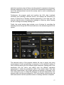
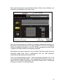
3.4 Main Labview Program and User Interface...............................................
Chapter 4: Results
4.1 Characterisation of elements and system.................................................
4.1.1 LCVR characterisation.................................................................
4.1.2 Characterisation of Polarisation State Generator………………..
4.2 Characterisation of the system..................................................................
4.2.1 Results for different media and comparison
to ideal response..................................................................................
4.2.2 Repeatability and Precision.........................................................
4.2.3 Analysis of system performance through
gradual variation of a single factor.......................................................
34
34
36
36
37
45
51
51
53
55
56
63
63
66
68
72
73
75
Chapter 5: Conclusions
5.1 System performance...............................................................................
5.2 System limitations...................................................................................
5.3 Future work.............................................................................................
5.3.1 Lock-In amplifier.............................................................................
5.3.2 Data acquisition card......................................................................
5.3.3 PEM based PSG............................................................................
5.3.4 Mechanical system.........................................................................
5.3.5 Readings for wider areas................................................................
5.3.4 Spectral range.................................................................................
77
77
78
78
79
79
79
79
80
References....................................................................................................
81
Appendix A....................................................................................................
84
Analysis for transmitted light intensity
for a dual photoelastic modulator system
Appendix B...................................................................................................
92
Transmission Laser Ellipsometer: Business Plan
v
List of Figures
Figure 1.1. Representation of linearly polarised light at 45°..................................6
Figure 1.2. Representation of circularly polarised light..........................................7
Figure 1.3. Representation of elliptically polarised light.........................................8
Figure 1.4 – Glan-Thompson prism.......................................................................9
Figure 1.5 – A quarter waveplate retarder.............................................................10
Figure 1.6 –Principle of operation of an LCVR......................................................11
Figure 1.7 – The components of a photoelastic modulator...................................12
Figure 1.8 – Polarimetric system based on photoelastic modulators....................13
Fig. 2.1 – Example of a rotating-element polarimeter...........................................18
Fig. 2.2 - Two mechanical rotation setups suitable for rotation of elements
in a polarimeter.....................................................................................................19
Fig. 2.3 – Dual PEM Stokes polarimeter...............................................................20
Fig. 2.4 – Rotating element Mueller polarimeter...................................................24
Fig.2. 5 – Complete Mueller polarimeter based on photoelastic modulators........24
Fig. 2.6 – Complete Mueller polarimeter based on liquid crystal variable
retarders (LCVR)..................................................................................................25
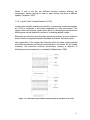
Figure 2.7 – Typical spectral response of a silicon photodiode............................28
Figure 2.8 – Photodiode operating modes............................................................29
Fig. 2.9 - Lock-In Amplifier Functional Block Diagram..........................................31
Figure 2.10 - Graphical representation of two sinusoidal signals with a
phase difference of 90° and the resulting multiplication.......................................32
Fig. 3.1 – Full Mueller polarimeter........................................................................37
Fig. 3.2 – Experimental setup used for the characterisation of the
photoelastic modulator..........................................................................................38
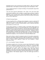
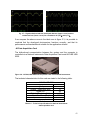
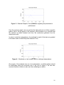
Fig. 3.3 – Ideal output of system for a retardance of half a wave
and 1.5 waves.......................................................................................................39
Fig. 3.4 – Output signals obtained using a New Focus photodetector
with a retardance of half a wave and 1.5 waves....................................................39
Fig. 3.5 – Basic current to voltage converter.........................................................40
vi
Fig. 3.6 – Current to voltage converter with a bandwidth of BW = 1.65 MHz
and dark current compensation............................................................................42
Fig. 3.7 – Signals obtained with the developed detector and the commercial
one........................................................................................................................43
Figure 3.8 – NI DAQ USB 6229 Data acquisition card from National
Instruments...........................................................................................................43
Figure 3.9 – Diagram of slot blade disc used for the chopper..............................45
Figure 3.10 – Schematic of the dual-photoelastic based full-Stokes
polarimeter............................................................................................................45
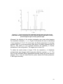
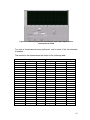
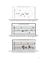
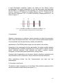
Figure 3.11 – Fourier spectrum of the modulated intensity signal
using the circular polarisation sensitive configuration for three
different states of polarisation: linearly polarised light and right
circularly polarised light.........................................................................................50
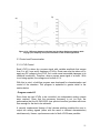
Figure 3.12 – Difference between calculated and incident Stokes
parameters while varying a) the ellipticity and b) the orientation of
the incident light beam...........................................................................................51
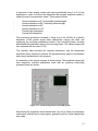
Figure 3.13 – Control program for dual LCVR system...........................................52
Figure 3.14 – Digital switch used to control the input of the reference
signal for the lock-in amplifier.................................................................................54
Figure 3.15 – Software simulation for the switching device....................................54
Figure 3.16 – Connection diagram for the system..................................................55
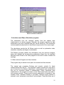
Figure 3.17 – Control window for Basic Serial Write and Read.vi..........................56
Figure 3.18 – Control panel for manual operation of system..................................57
Figure 3.19 – User interface for automatic measurement sequence......................58
Figure 3.20 – Implementation and control panel of the voltage sequence
for the LCVRs.........................................................................................................59
Figure 3.21 – Subvi which calculates the Mueller matrix from a given set
of four Stokes vectors.............................................................................................62
Figure 3.22 – Automatic measurement user panel, displaying the Mueller
matrix of the sample under study............................................................................62
Figure 4.1 – Labview program for controlling the input square signal used
to characterise the LCVR........................................................................................64
Figure 4.2. Comparison between the obtained curves for orientation....................65
vii
Figure 4.3. Comparison between the obtained curves for ellipticity of
outcoming beam.....................................................................................................65
Figure 4.4 Experimental setup for the polarisation state generator
based on two liquid crystal variable retarders.........................................................66
Figure 4.5. Experimental setup for the polarisation state analyser
based on two photoelastic modulators....................................................................68
Figure 4.6. Curves representing the last three stokes vectors for
each of the linear polarisations with varying orientation from 0° to 180°................69
Figure 4.7. Curves representing the last three Stokes vectors for each
of the elliptical polarisations oriented a 90° and ellipticities varying from
-1 to 1......................................................................................................................71
Figure 4.8. The sixteen Mueller Matrix elements, averaged throughout
five different measurements, along with their respective error for a /2
retarder...................................................................................................................74
Figure 4.9. The sixteen Mueller Matrix elements, averaged throughout
five different measurements, along with their respective error for a /4
retarder...................................................................................................................74
Figure 4.10. The sixteen Mueller Matrix elements, averaged throughout
five different measurements, along with their respective error for Air.....................74
Figure 4.11. Elements for the Mueller matrix corresponding to a quarter
waveplate retarder throughout a series of measurements with various
light intensities........................................................................................................75
List of Tables
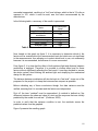
Table 3.1- Applied voltages to both LCVRs required to obtain all six main
polarisation states...................................................................................................37
Table 3.2 – Technical specifications for silicon photodiodes..................................40
Table 3.3 – Technical specifications for the AD823 Opamp...................................41
Table 3.4 – Technical specifications for National Instruments data acquisition
Card........................................................................................................................43
Table 3.5 – Sample list of ASCII commands for the Lock-in amplifier....................44
Table 4.1 – Results for LCVR characterisation.......................................................64
viii
Table 4.2. Applied voltages for generating various polarisation states
used for the complete system characterisation.......................................................67
Table 4.3. Stokes vectors for each of the generated orientations for
the linear polarisations in the system......................................................................69
Table 4.4 - Stokes vectors for each of the generated ellipticities at 90°.................71
ix
Thesis Title: “COMPLETE MUELLER POLARIMETER BASED ON LIQUID
CRYSTAL VARIABLE RETARDERS AND PHOTOELASTIC
MODULATORS”
Candidate: Eng. Alicia Fernanda Torales Rivera
Chairsperson: Dr. Geminiano Martínez Ponce / Dra. Cristina Solano
Program: Masters in Optomechatronics
The implemented Mueller polarimeter works in transmission and is constituted by
two modules: a polarisation state generator (PSG) and a polarisation state
analyser (PSA). The PSG is based on a dual system of liquid crystal variable
retarders (LCVR) set up in accordance to generate any state of polarisation by
combining the induced retardance in each. ON the other hand, the PSA is
constituted by a dual Photoelastic Modulator (PEM) system which in turn allows for
the measurement of the four Stokes parameters without the need to modify the
experimental setup.
The measurement for the 16 element Mueller matrix associated to a transparent
optical medium is achieved by using a single wavelength ( = 632.8nm). The
procedure consists on propagating a beam of light with four different polarisation
states (generated by the PSG) through the sample and to measure the polarisation
state in the outcoming beam with the PSA. The aforementioned provides a system
of equations which will in turn lead to details on all the sample’s linear anisotropies
such as linear and circular birefringence and linear and circular diattenuation. The
system uses a silicon photodiode as a means of detecting the incident beam and
its behaviour. The photoreceiver encompasses, along with the photodiode, a
preamplifying stage and a lock-in amplifier for signal detection and analysis. The
system is controlled via a computer and a data acquisition card from National
Instruments™. The control program was developed in Labview™ and allows the
user to take measurements either manually, step by step or with an automatic
sequence.
The applications for this measurement device include material analysis for the
development of optical devices, characterisation of optical tissue, detection of
polluting substances, and pharmaceutics quality control among many others.
1
Nombre de la Tesis: “POLARÍMETRO DE MUELLER COMPLETO BASADO EN
RETARDADORES
DE
CRISTAL
LÍQUIDO
Y
MODULADORES
FOTOELÁSTICOS”
Defensor: Ing. Alicia Fernanda Torales Rivera
Asesor: Dr. Geminiano Martínez Ponce / Dra. Cristina Solano
Postgrado: Maestría en Optomecatrónica
El polarímetro de Mueller implementado funciona en transmisión y esta compuesto
por dos módulos: un generador y un analizador de estados de polarización, PSG y
PSA, respectivamente. El PSG está constituido por un sistema dual de placas
retardadoras variables de cristal líquido (LCVR) dispuestos de tal manera que
pueden generar cualquier estado de polarización al combinar los retardos
inducidos en cada una. Por otra parte, el PSA esta formado por un sistema dual de
moduladores fotoelásticos (PEM) que permiten la medición de los cuatro
parámetros de Stokes sin modificar el arreglo experimental.
La medición de los 16 elementos de la matriz de Mueller asociados a un medio
óptico transparente se lleva a cabo utilizando una sola longitud de onda ( =
632.8nm). El procedimiento consiste en propagar un haz de luz con cuatro estados
de polarización diferentes generados por el PSG a través de la muestra y medir
los estados de polarización en el haz transmitido empleando el PSA. Lo anterior
proporciona un sistema de ecuaciones que llevará a la obtención de todas las
anisotropías lineales de la muestra bajo estudio (birrefringencia lineal / circular,
diatenuación lineal / circular). El sistema utiliza como dispositivo de detección un
fotodiodo de silicio con etapa de preamplificación y un amplificador de amarre de
fase para el análisis de la señal. El sistema es controlado por medio de una
computadora y una tarjeta de adquisición de datos de National Instruments™. El
programa de control desarrollado en la plataforma Labview™ permite al usuario
tomar las mediciones de manera manual, paso a paso, o con una secuencia
automática.
Las aplicaciones en donde las bondades de este instrumento de medición son de
gran utilidad incluyen el estudio de materiales para el desarrollo de dispositivos
ópticos, la caracterización de tejido biológico, la detección de contaminantes, el
control de calidad de fármacos, entre otros muchos.
2
Chapter 1
Introduction
1.1 On Polarisation and its importance in Science
Light polarisation is widely acknowledged to be one of the most important
properties of light (Collet, 2005), being broadly used in several applications in a
wide variety of fields, including Medicine, Holography, Biology, Pharmaceutics,
and Food Processing. This property has led to numerous discoveries and
technological breakthroughs all the way back to the 1600s (Goldstein, 2003).
According to Maxwell’s theory, light, as an electromagnetic wave, presents both
an oscillating electric field and an oscillating magnetic field. The former
oscillating at the same frequency than the latter, but with a perpendicular
orientation. Only the electrical field is considered when determining the
polarisation state of light.
1.2 Polarisation and Coherence
In 2005, Nobel Laureate R.J. Glauber proposes that the coherence condition is
fulfilled only if the light is totally polarised (Réfrégier, 2007). Additionally, Emil
Wolf (Pye, 2001) stated that there is an intimate relationship between
polarisation properties of a random electromagnetic beam and its coherence
properties.
Assuming that monochromatic light travels in sinusoidal waves, the amplitude
and phase of such waves can only be maintained constant throughout certain
amount of time. Afterwards, the amplitude is bound to vary the further it travels.
The period of time in which the phase of a light wave remains on average,
constant is known as coherence time.
Given that it is possible to define a polarisation state only when both
components of light maintain the same relative phase one with respect to the
other, it is possible to say that polarisation of light is only possible when the light
is coherent.
Furthermore, a single ray of light consists of two independent oppositely
polarised rays. When passed through a birefringent (doubly refractive) crystal,
such as calcite, two emerging rays can be observed. This is due to the fact that
in a birefringent crystal, these two rays experience different refractive indexes.
If then, a second crystal is used through which both rays pass through, by
means of rotation one of the beams can be completely extinguished, whereas
the other one’s intensity is maximised. By rotating the second crystal again,
another 90°, the first ray reappears at maximum intensity and the second one
vanishes. Finally, if the crystal is to be reoriented at an angle of 45°, the
3
intensities of the two rays are equal. These two rays are then said to be
polarised (Collet, 2005).
The two rays represent the “S” and the “P” polarisation states. The S and P
notations come from the German words for parallel (paralelle) and
perpendicular (senkrecht). This way, a light beam can be represented by two
components, the P polarisation component, usually denoted as E y and the S
polarisation component, denoted as Ex.
As a wave, light propagates sinusoidally throughout space at an angular
frequency . If we represent the maximum amplitudes of the two components
as Eox and Eoy and the phases as x and y, a beam of light can be represented
by the following equations:
Ex(z,t) = Eox cos(t – kz + x)
Ey(z,t) = Eoy cos(t - kz + y)
Where k = 2/, which is the wave number magnitude.
In the case in which the components have identical phases, one can obtain
linearly polarised light in several directions. It is possible to combine the
orthogonal components of linearly polarised light so as to produce other types
of polarised light.
Another case worth noting is when the components’ phases are 90° out of
phase with each other, whereas the amplitudes are exactly the same. This
results in circularly polarised light.
If neither of the conditions described above is met, then the light will present an
elliptical polarisation, which is considered to be the most general case. In order
to analitically visualise the above description, we shall briefly develop some
theory.
1.2.1 Linear Polarisation
Considering light as an electric field whose magnitude oscillates through time
and which is oriented along the polarisation axis, the polarisation is linear. Thus,
for light propagating along the z axis, it is possible to describe linearly polarised
light along the x axis as:
Ex = Eox sin[t – kz + o] i
(1.1)
And along the y axis as:
4
Ey= Eoy sin[t - kz + y] j
(1.2)
Where:
Eox,oy  Amplitude (electric field magnitude)
i  Unit vector along the x axis
j  Unit vector along the y axis
 = 2 ( = wave frequency)
k= 2/ ( = wavelength)
o = absolute phase
Hence, the electric field of linearly polarised light may be described as the
vector sum of Ex and Ey.
E = Ex + Ey
= {Eox i + Eoy j} sin[t – kz + o]
(1.3)
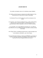
This configuration may be better visualised in the following figure, in which the
two orthogonal components are represented in blue and the resulting
polarisation in red.
5
Figure 1.1. Representation of linearly polarised light at 45°. a) isometric view. b) frontal view.
1.2.2 Circular Polarised Light
Consider the case in which both components are equal in magnitude, but 90°
(/2 rad) apart from each other in phase.
Ercp = Eo{sin[t – kz + o] i + sin[t – kz + o + /2] j}
= Eo{sin[t – kz + o] i + cos[t – kz + o] j}
(1.4a)
Elcp = Eo{sin[t – kz + o] i + sin[t – kz + o - /2] j}
= Eo{sin[t – kz + o] i - cos[t – kz + o] j}
(1.4b)
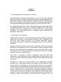
This configuration results in circularly polarised light, which can be better
visualised in the following figure:
6
Figure 1.2. Representation of circularly polarised light (represented by the arrows). a)
isometric view. b) frontal view.
As seen from the z axis, the electric field-representing vector has a constant
magnitude, but its orientation changes over time in such a way that the vector’s
head describes a circular route over time. Thus, the vector in the z=0 plane
seems to draw a circle clockwise when seen from the z+ side in front of the
origin.
Hence, this polarisation is called “left circularly polarised light”.
1.2.3 Elliptically Polarised Light
Elliptically polarised light may be considered as the general case of polarisation.
Again, if the phases are separated 90° from each other, but the component Ey ≠
0 and Ey < Ex, then the light will be elliptically polarised, with the major axis of
the ellipse directed along the x axis. If, on the other hand, E x ≠ 0 and Ex < Ey,
the major axis of the ellipse will be along the y axis. Hence, the ellipticity and
orientation of the polarisation ellipse will depend on the relative values of E x and
Ey and on their respective relative phases.
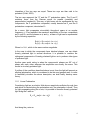
Similarly to circularly polarised light, the electric field vector of elliptically
polarised light forms an ellipse through time as seen from the z axis. It would
appear like a flattened spiral when seen from the xy plane (figure 3).
7
Figure 1.3. Representation of elliptically polarised light (represented by the arrows). a)
isometric view. b) frontal view.
Another possible way of obtaining elliptically polarised light is with different
phases of 0°, 90°, 180° and 270°, despite having equal amplitudes. Also if E x ≠
Ey and x≠y.
1.3 Polarising Elements
1.3.1 Linear Polarisers
Linear polarisers can transmit light, whose electric field vector oscillates within
the plane that contains the polariser’s axis. This plane’s orientation can be
varied by rotating the polariser. If the plane is horizontal, the polariser is called
a horizontal linear polariser. If the electric field of the light passing through the
polariser’s got a component that is orthogonal to the polariser’s transmission
axis, it will suffer attenuation of said component.
Whenever a linear polariser is placed in front (or behind) another linear
polariser, both of them with their axes placed orthogonally to each other
(crossed polarisers), all light should ideally be extinguished.
1.3.2 Glan Thompson Prism
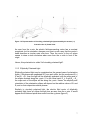
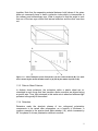
The Glan Thompson prism configuration is shown in figure 1.4. The prism is
polished in such a way that the optical axis is located in the plane of the
entrance face as well as parallel to the diagonal cut. This prism has several
advantages. Since light enters the crystal normal to the surface and to the optic
axis, both the ordinary and the extraordinary rays move normal to the surface,
without deviating. For traditional Glan-Thompson prisms, both halves are glued
8
together. Note that the separating material between both halves of the prism
does not necessarily have to have a refraction index which is intermediate to
the ordinary and extraordinary rays. What is required is that the angle is such
that one of the two rays suffers total internal reflection and the other one does
not.
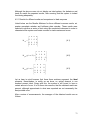
Figure 1.4 – Glan-Thompson prism. Perspective (A) and cross-sectional (B). The optic
axis is shown by the double headed arrows in (A) and by the matrix of points in (B).
1.3.3 Dichroic Sheet Polariser
In dichroic sheet polarisers, the molecules within a plastic sheet are reorientated in such a way that their transition dipole moments are aligned along
a specific axis. Thus, light polarised in this same axis is absorbed whereas light
polarised orthogonally is transmitted.
1.3.4 Retarders
Retarders make the absolute phases of two orthogonal polarisation
components to be varied after propagation, as a function of thickness. A
common example is the quarter wave plate retarder (/4), which increases by
90° the phase of a linear polarisation relative to another.
9
Retardance is an effect caused by the refractive index. As light is transmitted
from vacuum to another material, the speed of light is reduced by a factor of 1/n,
where n is the refractive index of the material. Since the frequency remains
constant when the light passes from one medium to another, this results in a
faster variation of the phase angle of light within a body than in vacuum.
Consequently, any transparent body increases the phase of light in comparison
to the one it has outside the body.
A body that provokes retardation between orthogonal components in the same
degree, for any given polarisation, regardless of the orientation of propagation,
is said to be isotropic in nature.
1.3.5 Birefringent Plate Retarders
Birefringent plate retarders can cause a phase difference between two
orthogonal polarisations.
It is also possible to modify the polarisation state using anisotropic absorption
elements.
Figure 1.5 – A quarter waveplate retarder.
Consider a linearly polarised light beam that passes through a birefringent
crystal or waveplate. Given that linearly polarised light is formed by two
components (Eq. 1.3), this causes the two components to experience slightly
different refractive indexes.
If we have a plate of thickness d and assuming that the wavelength  remains
the same before and after passing through the medium, the wavelength in the
crystal may be defined as /n, where n is the crystal’s index of refraction. Thus,
the total number of waves in the plate is d/(/n). If each of the mutually
orthogonal components is affected by a different refraction index, the phase
difference after exiting the plate can be defined as:
(1.5)
10
Where ni and nj are the two different refractive indexes affecting the
components, hence causing for them to pass through the plate at different
speeds (Tompkins, 2005).
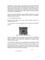
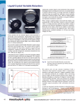
1.3.6 Liquid Crystal Variable Retarder (LCVR)
Liquid crystal variable retarders are real-time, continuously tunable waveplates.
An LCVR is composed of two plates separated by a few micrometers. This
space is filled with nematic liquid crystal, which is a birefringent material whose
birefringence can be adjusted by means of a variating applied voltage.
Electrodes are located in specific places among the retarder, so as to enable an
electric field to be applied between both plates and hence, the liquid crystal.
Upon application of the voltage, the molecules within the liquid crystal gradually
reorientate themselves until they are perpendicular to the plates. As the voltage
increases, the molecules continue reorientating, causing a reduction in
birefringence and consequently, in retardation (Meadowlark, 2009).
Figure 1.6 – Schematic representation of the principle of operation of an LCVR
11
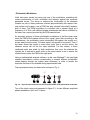
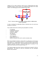
1.3.7 Photoelastic Modulator (PEM)
A photoelastic modulator causes a phase shift between the orthogonal
components of a light beam to change sinusoidally as a function of time. This
phase shift is obtained by making the two perpendicular components of light
pass through a waveplate at different speeds. This is achieved by inducing a
time-varying birefringence by way of a time-varying stress in a normally
isotropic material. An isotropic material will become anisotropic when stressed
and will thus induce the same kind of birefringence as an anisotropic crystal like
calcite.
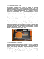
A picture of the constituting elements of a photoelastic modulator is shown in
figure 1.7. A piezoelectric transducer is a block of crystalline quartz cut at a
specific orientation (-18°, Xcut).
A metal electrode is deposited on each of two sides and the transducer is cut in
such a way that it resonates at a specified frequency F. The resonance is
uniaxial and is directed along the long axis of the crystal. A block of fused
quartz is cemented to the end of the transducer. The length of the fused quartz
is such that it also has F as the fundamental longitudinal resonance. When both
elements are cemented together, resonance of the transducer causes a
periodic strain in the fused quartz (Jellison, 2005).
Figure 1.7 – The components of a photoelastic modulator
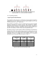
1.4 Dual PEM Systems in Polarimetry
A dual Photoelastic modulator system can obtain all 16 elements of the Mueller
Matrix (provided the four incident polarisation states of the incoming beam are
known), which describes the polarisation properties of a material (Goldstein,
2003). The typical configuration for such an ellipsometer would be tuning the
first PEM, P1, at frequency F1 and orientation of 0°, and the second PEM (P2)
tuned at frequency F2 (where F2 is slightly different from F1). Furthermore, P2
must have an orientation of 45°. P2 is then followed by a linear polariser at 0°,
as shown in figure 1.8.
12
Figure 1.8 – Polarimetric system based on photoelastic modulators(PEM1 y PEM2).
A is a linear polariser (analyser).
1.4.1 Applications of a Dual Modulator System
Whether in transmission or reflection, certain materials can affect the
polarisation state of light that interacts with them. This is due to intrinsic
qualities and properties of said materials such as optical activity, chirality
and reflectivity.
Applications for Dual PEM Systems range from the medical to the military.
Depending on the wavelength and other parameters, the system enables
analysis and characterisation of different materials (most of them organic in
nature, but also certain reflecting materials). Such materials are used in
medical analysis, holography, food processing and pharmaceutics, among
others.
Dual PEM polarimeters are used in astronomy to study light polarisation
from nearby stars and sunspots.
Another useful application of this system is in optical fibres. When a fibre is
bent, it generates mechanical stress, which in turn causes the polarisation
state of the light travelling through the fibre to change. Light polarisation may
also vary depending on the environment the fibre is in. Polarimeters are
hence used to monitor the polarisation state of light coming out of the fibre
(Hinds Instrument, 2005).
Intrinsic qualities of materials have an effect on the way light interacts with
them. Properties and characteristics such as stress, defects, reflectivity, and
polarisation loss may be determined with the instrument by measuring the
polarization state of light after passing through a material.
Other applications include thin film characterisation as well as laser test and
measurement.
13
1.5
Polarisation in Nature
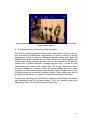
1.5.1 Why is the sky blue?
In other planets and satellites in outer space, the sky appears black and the
stars are visible throughout all day, regardless of the position of the Sun.
Nevertheless, here on Earth, the daytime sky appears blue and stars are not
visible. Whereas during night when the Sun is set, the stars are clearly
visible and the sky appears to be black. Why is this?
John Tyndall explained this phenomenon by showing that scattering of
sunlight, thus polarising it to a certain degree, takes place in the upper
atmosphere (Pye, 2001). Furthermore, he demonstrated that small particles
in the atmosphere scatter light of short wavelengths more strongly than
those of larger wavelengths. Thus, the blue color is predominantly scattered
rather than say, the red one. Lord Rayleigh further estimated that the
atmosphere need not necessarily contain solid or liquid particles for the
scattering to occur. A large enough amount of gas molecules will also suffice
for blue light to be scattered.
As it may be surmised, UV light, being shorter in wavelength than blue, is
scattered even more strongly, and although the human eye cannot see it,
several other animals are able to detect near-UV light and use it for different
survival purposes.
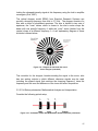
1.5.2 Seeing Polarisation
Besides UV-light, certain animals, mostly insects, are also able to detect
polarisation. Fifty years ago, Karl von Frisch studied the bees’ navigation
abilities. He discovered that bees used the orientation from the sun to tell their
kin the location of food sources. When an explorer bee leaves the hive in
search of food, it locates the position of the sun and can travel relatively large
distances up to nearly 4 hours away from the hive before heading straight
back. Nevertheless, the Sun’s position will obviously change throughout that
period of time. In addition, Frisch also noted that bees are able to navigate
accurately even when the Sun is covered by a cloud or mountain, thus
realising the Sun’s position isn’t the bees’ true compass, but rather the
polarisation pattern in the sky, determined in turn, by the Sun itself.
Through experimentation with Polaroid film, Frisch was able to prove his
theory, and proposed that each segment in the eight-segmented bee eye is
more sensitive to one specific direction of polarisation, thus enabling the bees
to detect different orientations.
14
Ants are also able to discriminate polarisation in sunlight (Pye, 2001).
Experiments on desert ants have been carried out in their natural habitat.
These insects often forage wide desertic areas in search of food, with no
landmarks to guide them back to their nest. If, for instance, the entire sky is to
be obscured by a cardboard box, the ants’ pathway becomes erratic,
rendering the insects unable to find their way back. In other experiments, the
sunlight was shielded from the ants, and in its stead, a reflection of the sun
was projected toward the insects. The result was a direction reversal of their
course.
It is not only insects that can see polarisation and use it in their daily lives.
Research with molluscs has also been carried out with results suggesting they
are also able to detect it. Exactly what use polarisation is to them is as yet
unknown, but scientists have theorised it may be used to their advantage in
spotting food. Some small fishes they feed on, have reflecting scales,
imitating the reflections of light in water, rendering them nearly invisible to
most predators. However, these reflections in the fishes’ scales do not match
in terms of polarisation, to the scattering produced by incident light on water,
thus enabling the octopus to distinguish its prey with relative ease.
Finally, a crustacean species, commonly known as “Peacock Mantis Shrimp”
has been reported to be able to detect circularly polarised light, better in fact,
than any man-made optical device currently in existence (Matson, 2009).
1.5.3 Polarisation in Medicine
Applications in tissue studies
Biological media comprise two large categories in which the different tissues
and fluids may be divided (Tuchin, 2006). The first one, known as “Weakly
Scattering Media”, which transparent tissues and fluids such as cornea,
vitreous humour and crystalline lens. The second one, the “Strongly
Scattering Media” includes opaque or turbid tissues and fluids like the skin,
brain, blood and lymph.
Biological tissues are rendered transparent in the near-infrared (NIR) region of
the spectrum, due to the absence of absorbing chromophores in this spectral
range. A chromophore is a chemical and part of a molecule that absorbs light
“with a characteristic spectral pattern” (Tuchin, 2006), hence being
responsible for the molecule’s color.
However, biological tissues produce rather strong scattering in this spectral
region, making it difficult to obtain clear images of inhomogeneties within the
sample, making them hard to localise. Due to this, classic imaging is virtually
useless for studying this kind of media and specialised techniques need to be
used when analysing biological tissues.
15
In certain tissues for example, the degree of polarisation of transmitted or
reflected light is measurable regardless of the tissue’s thickness, whereas in
other media, reflected or transmitted light depolarises much too fast for
obtaining useful information out of it degree of polarisation. Still, information
about the structure and birefringence of its components may be obtained by
measuring the degree of depolarisation of initially polarised light passing
through a tissue sample.
However, it is not only from these polarisation properties that useful
information can be obtained. Several tissues, retina and tooth enamel among
them, present properties such as linear birefringence and optical activity due
to their composition and nature. Collagen, keratin or glucose being present in
them.
Considering all the aforementioned, it is safe to say that biological tissues and
fluids are, in most cases, polarising materials to some extent. These
properties are expected to enhance the improvement of the current
techniques in medical tomography and other diagnostic methods (Tuchin,
2006).
Other important medical applications which use polarisation include glucose
and bacteria sensing.
This work will not delve on the history of polarisation studies, but rather in the
nature of the phenomenon and its applications.
16
Chapter 2
Review of Literature
2.1 Introduction
Several instruments for measuring polarisation of light, i.e., polarimeters and
ellipsometers, have been proposed throughout the years (Guo, 2007; Wang, 2005;
Oakberg, 2005; Giudicotti, 2007; Aspnes, 1976, Azzam, 1977; Ord, 1977). This
kind of systems, in which this work will focus, enable measurement of light
polarisation properties before and after light has gone through or has been
reflected by a sample.
Polarimeters also enable the study and analysis of parameters such as the
complex refractive index and thickness of thin films.
The term “Polarimetry” describes the polarisation properties of light. Hence, a
polarimeter measures and analyses such properties from a beam of light. In its
simplest form, a polarimeter is composed of a polarisation state generator and a
polarisation state analyser. Together, they constitute a closed-loop system, in
which control and feedback is provided to and from the system. For this project, we
will use the terms “polarimeter” and “ellipsometer” as equivalent.
In addition, polarimeters may also be classified as Stokes Polarimeters and Mueller
Matrix Polarimeters. The former merely describes the polarisation state of light
through the Stokes Parameters, whereas the latter, enables the description of the
polarisation properties of a material in reflection or transmission.
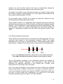
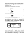
The Stokes vector is a set of four parameters which together define the polarisation
state of a given beam of light. The vector is defined as follows:
 S0 
 
 S1 
S 
 2
S 
 3
(2-1)
Where S0 represents the total light intensity of the beam, regardless of the
polarisation state, S1 refers to the linearly polarised components either vertically or
horizontally oriented. S2 also refers to the linearly polarised components but with
±45° of orientation, and finally S3 represents the right and left circularly polarised
components.
17
Furthermore, from these parameters it is possible to obtain the degree of
polarisation, ellipticity and orientation of the analysed beam.
Besides there being different measuring systems, there are also different
components and configurations used in them (Aspnes, 1976). These mainly
include modulating elements, detection devices and data processing systems. All
of them with both advantages and disadvantages.
An analysis of the most commonly used systems and elements is presented. Note
that only the systems that are able to measure all four Stokes components will be
mentioned.
Furthermore, besides the polarimetry system itself, an appropriate data processing
system ought to be implemented in order to interpret the results correctly, calculate
the Mueller Matrix and finally obtain the polarisation state and properties from the
sample under study.
2.2 Polarimeters that enable measurement of the 4 Stokes Parameters
2.2.1 Rotating element polarimeters
The elements that constitute these systems are all linear retarders and polarisers .
Fig. 2.1 – Example of a rotating-element polarimeter
These elements are usually rotated by mechanical or electromechanical means.
Measurements need to be forcibly taken periodically with a rotation at a continuous
speed or making pauses at periodic intervals to take each measure. The former
method is undeniably the most accurate and fastest one, as it provides a greater
number of measurements, but the detection and data acquisition need to have a
very fast response.
Stepper motors or servo motors are often the preferred choice for these
polarimeters, though systematic errors and encoder performance may affect the
precision and reliability of the obtained data (Giudicotti, 2007). Different mechanical
18
setups have been used, usually involving a quarter-wave plate retarder and/or an
analyser mounted on a rotation stage, driven by a motor. Two of these setups are
shown below on figure 2. The mechanism on the left shows a motor-band system
that enables automatic rotation of the base in which the waveplate is mounted. The
second mechanism proposes a system of two gears. One of them is mounted on
the motor, whereas the second one serves the double purpose of rotating stage
and mount for the retarder. Needless to say, the latter example is more accurate,
as long as both gears are perfectly compatible in matter of diameter/number of
teeth relationship. Nevertheless, at least the gear in which the waveplate is
mounted ought to be custom – made for the plate to fit properly in the exact centre.
Mini-steppers have also been used successfully, providing greater accuracy in the
measurements (Ord, 1977).
The measurements are then taken using the angular position of the transmission
axis of the rotating element as reference, hence determining the initial point of the
graphic generated by the acquired data, thus simplifying the mathematical analysis.
Whenever more than one element is rotating, they must both do so at the same
frequency (Azzam, 1977).
The mathematical analysis for these type of system usually encompasses Fourier
analysis of the recorded signal (Goldstein, 2003), though a weighted least-square
best fit has also been proven efficient (Giudicotti, Brombin, 2007).
Finally, it must be stated, that when these systems are used as ellipsometers, they
are of no real use for samples undergoing rapid changes.
Fig. 2.2 - Two mechanical rotation setups suitable for
rotation of elements in a polarimeter.
2.2.2 Oscillating element polarimeters
These systems rotate the polarisation of light using an electro or magneto-optical
device such as a Faraday cell (Goldstein, 2003). If the plane of polarisation is
19
rotated in the cell, the effect would be the same as mechanically rotating the
elements in a rotating element polariser by a proportional angle.
As stated in last chapter, these cells may be driven by a periodic voltage signal,
thus forcibly requiring a signal generator. The most widely used devices are the
liquid crystal variable retarders (LCVRs).
For the specific case of LCVRs, two of them are required to measure all four
Stokes parameters (Meadowlark optics, 2005).
These systems provide for a significantly faster response than those previously
described, thus proving far more efficient when used with rapid-changing samples
(Aspnes, 1976). Nevertheless, when calibrating and taking measurements, care
must be taken to preserve a constant temperature level, since liquid crystals are
sensitive to temperature variations and may affect the obtained results (Carey,
1996).
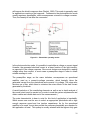
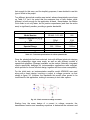
2.2.3 Phase modulation polarimeters
These systems use modulators that are controlled by an electrical signal. The most
commonly used element is the photoelastic modulator (PEM). The system
presented here is of this type. It consists basically of a dual phase modulator and a
fixed analyser. A diagram of the element setup is presented in the following figure:
Fig. 2.3 – Dual PEM Stokes polarimeter, which measures all four Stokes parameters,
where PEM1 and PEM2 are photoelastic modulators and A denotes an analyser.
The two photoelastic modulators in the polarisation analyser are operated at
slightly different resonant frequencies, thus generating a “beat signal” that
modulates the polarised component of the incident light. Typically, these
frequencies are in the range of tens of kilohertz.
One of the main advantages of this system over both rotating and oscillating
element polarimeters is speed. Although they all require an electrical signal for
control and acquisition purposes, the response of PEMs is significantly faster than
any motor or liquid crystal cell. Nevertheless, the overall cost of the device
increases significantly given the high cost of each modulator.
20
These systems, though popular as a dual PEM system, are used in different
physical setups involving axis orientation.
2.3 The Mueller Matrix
Consider the Stokes vector from equation (2-1), with its four parameters
represented by:
 S0 
 
 S1 
S 
 2
S 
 3
which together represent the polarisation properties of a given light beam.
Let us now assume that the beam interacts with a polarising medium whose
characteristics are at present unknown. The emerging beam will then be
represented by a new Stokes vector, which we shall represent by:
 S0 ' 
 
 S1 ' 
 S '
 2
 S '
 3
(2-2)
If we represent each of the Si’ (where i = 0,1,2,3) parameters as a linear
combination of the original Si parameters, we may obtain the following relations
(Goldstein, 2003):
S0'  m00S0  m01S1  m02S 2  m03S3
(2-3a)
S  m10S0  m11S1  m12S 2  m13S3
(2-3b)
S  m20S0  m21S1  m22S 2  m23S3
(2-3c)
S3'  m30S0  m31S1  m32S2  m33S3
(2-3d)
'
1
'
2
In matrix form, (2-3) can also be expressed as,
 S 0 '   m00
  
 S1 '   m10
 S '   m
 2   20
 S '  m
 3   30
m01 m02
m11 m12
m21 m22
m31 m32
m03  S 0 
 
m13  S1 
m23  S 2 
 
m33  S 3 
(2-4)
21
or
(2-5)
S '  MS
Where S and S’ are the Stokes vectors and M is the 4 x 4 matrix known as the
Mueller Matrix.
Whenever an optical beam interacts with matter, whatever the media, its
polarisation state nearly always suffer changes. Depending on specific properties
of the material, the polarisation state of the incident beam varies accordingly.
Some of these variations in polarisations state include changes in the amplitude,
phase, direction of the orthogonal field components, and transference of energy
from polarised states to the unpolarised state (Goldstein, 2003). Each of these
elements may be in turn, represented by a particular Mueller Matrix.
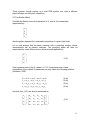
For instance, a linear polariser, with its axes along the x and y directions may be
represented by the following Mueller Matrix:
 p x2
 2
1  px
Mp  
2


where,
and
 p y2
 p y2
0
0
p x2  p y2
p x2  p y2
0
0
0
0
2 px p y
0
0 

0 
0 
2 p x p y 
(2-6)
0  px, y  1
px and py are the attenuation coefficients of the polariser.
For simplification purposes, an alternate notation may also be used, where the
same Mueller Matrix defined in (2-6) can be rewritten as:
A

B
Mp 
0

0

B 0 0

A 0 0
0 C 0

0 0 C 
(2-7)
Where,
22
A
1 2
( p x  p y2 )
2
(2-7a)
B
1 2
( p x  p y2 )
2
(2-7b)
C
1
(2 p x p y )
2
(2-7c)
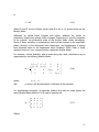
Furthermore, each of the Mueller Matrix elements describes a different property of
the material it represents. Among such properties, it is possible to determine the
diattenuation (differential attenuation of orthogonal polarisations for both linear and
circular polarisation states), depolarisation coefficient, and linear retardance
assuming a thin film. Thus, the properties are represented as follows (Tuchin, 2009;
Kim, 1987):
p
 ( LD0 )  ( LD45 ) (CD) 

  ( LD )
p
(CB )
( LB45 ) 
0

m
 ( LD45 )  (CB )
p
 ( LB0 )


 ( LB45 )
( LB0 )
p 
 (CD)
(2-8)
Where,
P
LD0
LD45
CD
CB
LB0
LB45
=
=
=
=
=
=
=
Isotropic Absortion
Linear Diattenuation (0° or 90°)
Linear Diattenuation (±45°)
Circular Diattenuation
Circular Birefringence
Linear Birefringence (0° or 90°)
Linear Birefringence (±45°)
However, not all materials alter polarisation in the same way or indeed, in the same
degree. When it is required to analyse the polarising properties of a specific
material, a Mueller Matrix polarimeter is then used, which enables the
measurement of the different elements that constitute the Mueller Matrix that
represents said material, thus providing useful information on properties and
characteristics of the sample under study.
2.4 Mueller Matrix Polarimeters
Mueller Polarimeters aim to measure the elements from the 4x4 Mueller Matrix of a
given sample either in reflection or transmission. A polarimeter is said to be
23
complete if it measures all 16 elements from the matrix, whereas an incomplete
polarimeter merely measures a part of the matrix. Given that different elements
from the Mueller Matrix represent different properties of the material under study, it
is sometimes unnecessary to measure all 16 elements, and thus, an incomplete
polarimeter may be used for such cases.
In order to have a complete measuring system, the instrument must encompass
two stages, both functioning in strict synchronicity. The first stage consists of a
complete polarisation state analyser (PSA) and the second, a complete
polarisation state generator (PSG). The reason for both stages is clear: it is
necessary to know which polarisation state is entering the sample as well as which
state is exiting it, thus enabling calculation of which polarisation changes occurred
during the process.
As in the case of Stokes polarimeters, there are different elements available for
both the PSA and PSG stages, these being either rotating elements or phasemodulating devices. As in the previous section, only complete Mueller polarimeters
will be mentioned.
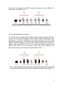
2.4.1 Rotating element polarimeter
A rotating element polarimeter capable of measuring all 16 elements of Mueller
matrix is formed by a fixed polarimeter, followed by a rotating retarder, which
together constitute the PSG stage. The sample is located in the middle of both
PSG and PSA stages. The PSA stage is similarly formed by a rotating retarder,
followed by a fixed analyser. The following diagram illustrates this setup:
Fig. 2.4 – Rotating element Mueller polarimeter, where “P” denotes the polariser, “A” is an
analyser, and R1 and R2 are retarders.
2.4.2 Phase-Modulating Polarimeter
This system uses photoelastic modulators (PEM) as a means for controlling and
determining the state of polarisation of a light beam. The arrangement consists on
a fixed polarimeter oriented at 0°, a PEM oriented at 45°, followed by a second
PEM oriented horizontally. These elements together constitute the PSG stage of
the system. Again, the sample is located between the PSG and PSA. The PSA
24
then follows the sample with a PEM oriented horizontally, a second PEM at 45°
and finally, a fixed analyser at 0°.
Fig. 2.5 – Complete Mueller polarimeter based on photoelastic modulators.
The same notation as in the previous figure is used for the constituting elements.
2.4.3 Oscillating Element Polarimeter
Yet another setup for measuring the Mueller matrix has been proposed based on
the use of four LCVRs (De Martino, 2003; Uberna, 2006). Although still under
development, the results obtained thus far seem promising. The PSG stage
generates a sequence of four different retardations before the beam enters the
sample. Different retardation values have been tested, each based on the work of
different authors and criteria. A set of four values has been proposed by the
authors, with which the most accurate results have been obtained. The
experimental setup for the instrument is presented as follows,
Fig. 2.6 – Complete Mueller polarimeter based on liquid crystal variable retarders (LCVR). 
and its different subindexes represent various possible orientations of the elements.
25
2.4.4 Applications of a Mueller Polarimeter
Whether in transmission or reflection, certain materials can affect the polarisation
state of light that interacts with them. This is due to intrinsic qualities and properties
of said materials such as optical activity, chirality and reflectivity.
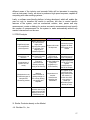
Applications for Dual PEM Systems range from the medical to the military.
Depending on the wavelength and other parameters, the system enables analysis
and characterisation of different materials (most of them organic in nature, but also
certain reflecting materials). Such materials are used in medical analysis,
holography, food processing and pharmaceutics, among others.
Dual PEM polarimeters are used in astronomy to study light polarisation from
nearby stars and sunspots.
Another useful application of this system is in optical fibres. When a fibre is bent, it
generates mechanical stress, which in turn causes the polarisation state of the light
travelling through the fibre to change. Light polarisation may also vary depending
on the environment the fibre is in. Polarimeters are hence used to monitor the
polarisation state of light coming out of the fibre (Hinds Instrument, 2005).
Intrinsic qualities of materials have an effect on the way light interacts with them.
Properties and characteristics such as stress, defects, reflectivity, and polarisation
loss may be determined with the instrument by measuring the polarisation state of
light after passing through a material.
Other applications include thin film characterisation as well as laser test and
measurement.
2.5 Detection Devices: Different Types of Photon Detectors
2.5.1 The Photomultiplier Tube
A typical photomultiplier tube consists of a vacuum tube containing a
photosensitive cathode followed by a series of electrodes (known as dynodes) that
collect and multiply the photocurrent generated in the cathode (Jonasz, 2009). A
voltage of the order of hundreds of volts is distributed between the electrodes of
the multiplier by a voltage divider network. A photon that strikes the photocathode
ejects an electron with the quantum efficiency of less than one fourth. Such
electron is then accelerated by the potential differences between the cathode and
the following electrode. The impact with said electrode results in the ejection of
several next-generation electrons. This electron multiplication continues for each of
the following dynodes, ending up in the anode, where the electrons are collected.
The overall process hence provides for an approximate of 106 electron gain.
26
2.5.2 Photodiodes
Sensing devices for polarisation measuring systems require a high-speed, lownoise response. Since the system presented in this work is to measure a single
light beam, we will focus on photodiodes as the preferred means of measuring light
intensity.
Photodiodes generate a small electrical current, which is proportional to the level of
the illumination incident on its surface.
There are two types of photodiode available for this kind of application: the PIN
photodiode, which can detect signals within a significantly wide spectral band, and
the avalanche photodiode, which has a faster response (Graeme, 1995).
Nevertheless, controlling the second type presents a somewhat greater challenge.
The photodiode to be used must be carefully selected in accordance to the signal
characteristics, such as amplitude and frequency. Not all photodiodes will be able
to detect a signal at a high frequency, nor will they be equally sensitive to all
wavelengths. Also, operation conditions should be taken into account so as to
minimise possible electrical noise and temperature variations during
measurements.
The main properties to keep in mind while choosing a suitable photodiode are
junction capacitance (Cj), dark current, spectral range, active area, and response
time (Graeme, 1995).
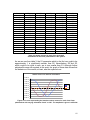
Spectral Response
The current generated by a given level of incident light varies with wavelength. The
relation between photoelectric sensitivity and wavelength is referred to as the
spectral response of the photodiode.
The operating wavelength for this stage of the project is that of  = 632.8nm, which
corresponds to the red color. Bearing this in mind, a silicon photodiode was chosen
due to its high sensitivity to red light.
In the following figure, a typical spectral response curve of photodiodes made of
different materials is presented (Johnson, 2004), in which the diode’s sensitivity
along a specific range of the spectrum may be seen. Notice that, according to the
graph, silicon photodiodes provide a fairly good responsivity along the red part of
the spectrum, making them suitable for the application at hand.
27
Figure 2.7 – Typical spectral response of a silicon photodiode.
Dark Current
It is a small current that flows when a reverse voltage is applied to a photodiode, i.e.
when the diode is used in photoconductive mode, even when no illumination is
incident on the diode. This current adds noise to the overall signal and must
therefore be minimised as much as possible.
Active Area
Physically, the active area refers to the amount of surface in the photodiode that
detects illumination. It is directly related to yet another characteristic, which is the
junction capacitance (cj). The smaller the active area is the smaller the junction
capacitance, which in turn provides for a greater frequency bandwidth (Graeme,
1995).
Mode of Operation
Any photodiode may be used in one of two different operating modes, the
photovoltaic and the photoconductive. In the former one, the photodiode functions
as a current source, simply changing light to an electric signal. On the other hand,
the photoconductive mode requires an inverse voltage to be applied to the diode.
This mode provides a greater linearity and frequency response, but is more
susceptible to noise and dark current (Jung, 2002). By applying and inverse
polarisation to the photodiode, the junction capacitance is reduced, which in turn
28
will improve the diode’s response time (Rashid, 1999). This mode is generally used
for applications requiring a fast response. Furthermore, the photoconductive mode
usually requires a preamplifier, which encompasses a current to voltage converter.
Thus, the linearity is lost after the conversion.
Figure 2.8 – Photodiode operating modes
In the photoconductive mode, it is possible to read either a voltage or current signal.
However, the generated electrical current is a linear function of the light intensity,
as opposed to the voltage response. Since most devices are designed to reading
voltage rather than current, in most cases a preamplifier stage in order to obtain
suitable readings in volts.
The preamplifier stage, as the name indicates, encompasses an operational
amplifier used as a current-to-voltage converter, which basically takes the
generated current from the photodiode and converts it to voltage. This stage also
functions as a filter, which aims to minimise the noise effects of the dark current
generated by the diode.
A careful selection of the constituting elements as well as an in depth analysis of
the overall circuit must be carried out in order to meet the system requirements and
obtain usable and reliable data out of the measurements.|
The main characteristic to bear in mind for this kind of application is bandwidth.
Which means one must be sure to select an appropriate photodiode with a high
enough response speed and low junction capacitance. As for the operational
amplifier to be used, it must also provide the necessary bandwidth one requires for
the application at hand. This opamp is usually selected with the highest unity gain
29
bandwidth product to input capacitance as possible (Graeme, 1995). The unity gain
bandwidth refers to the frequency at which unity gain occurs (Neiswander, 1975).
A more detailed description of analysis and design of the preamplifier stage will be
presented later on.
It has also been proposed (Neiswander, 1975, Fjarlie, 1977) that under harsh
environmental conditions, such as airborne or space borne monitoring, it might be
advisable to cool the entire circuit, diode and preamplifier stage included up to
200K. It has been reported that by doing this, dark current and other noise sources
may be actively suppressed.
2.6 Data Processing System
A Lock-in Amplifier (LIA) is a filtering system designed to acquire a particular AC
signal buried in noise or other signals and “extract” it from the rest, providing its
amplitude and phase. A reference sinusoidal signal, tuned to frequency and phase
of the desired one must be used.
Though signal generators or oscillators provide a reasonably stable signal, the
generated frequency varies by a few hertz through time. For this application, this
variation will not do, since we are aiming to “lock” the signal that is buried in noise.
Therefore, a phase locked loop (PLL) is also required to ensure that the reference
signal is precisely tuned and whose frequency is continuous. Basically, the PLL,
along with passive components with calculated values, is fed the sinusoidal signal
at a specific frequency. The circuit then feeds back the signal to the PLL and
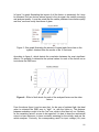
stabilizes the frequency, so as to ensure that it is fixed at the desired value.
Care must be taken to select the adequate values for the passive components.
Otherwise, the obtained frequency will not match the desired one. Formulae have
been provided for this purpose, and whenever the results render a non commercial
value for resistors and/or capacitors, trimpots are often advisable to ensure
frequency accuracy.
2.6.1 Lock-in Amplifier: Principle of Operation
The reference signal is fed to the lock in via one input channel and to a phase
locked loop, whereas the noisy signal and fed to another one. The noisy signal
then enters an optional amplifying stage (because usually the amplitude of the
desired signal is too small, usually in the range of mili or nanovolts). After the
amplification, the signal is sent to two separate stages. One stage directly
multiplies (or mixes) the noisy signal with the reference signal. The other one also
multiplies the noisy signal, but this time with the reference signal 90° out of phase.
So for instance, if the reference signal is a Sine, this other signal would be a
Cosine.
30
Both outputs are then fed to low-pass filters, tuned to eliminate all AC components,
and keep only those with frequencies close to zero, which would be the DC
component.
The actual process and complete circuit is somewhat more complex than the
description above. Since the signal may be buried in several others with various
frequencies, both greater and smaller, more than one filter may be required, either
low-pass or high-pass after the gain stage and others just before the final output.
Finally, a band-suppressing notch filter is sometimes recommended to be used
right after the amplifying stage to eliminate a reduced range of specific frequencies
whose amplitude is greater or equal to the one that is being extracted, yet
significantly apart in frequency terms from the desired signal (otherwise, one might
accidentally eliminate the signal along with the unwanted noise).
It must also be noted that the process of phase-sensitive detection demands an
exact phase synchronisation between the reference signal and the modulation of
the light beam (Chabay, 1975). With this in mind, it is advisable to use the very
same electrical signal that is driving the photoelastic modulators as the reference
for the lock-in.
A block diagram of the main stages of a lock-in amplifier is presented in figure 1.9:
Fig. 2.9 - Lock-In Amplifier Functional Block Diagram
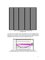
Phase sensitive detectors, shown in the above figure, measure the phase
difference between two signals of the same frequency. It does so by multiplying
31
both signals and thus obtaining a DC signal proportional to the phase difference
between the signals. For two square signals at a low frequency, an XOR gate will
suffice to achieve this. Nevertheless, for higher frequencies in sinusoidal
waveforms, a more specialised circuit is required. The IC AD633 is an analog
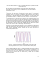
multiplier designed for this purpose.
Figure 2.10 - Graphical representation of two sinusoidal signals with a phase difference of
90° (left) and the resulting multiplication (right).
2.6.2 Basic Theory
Mathematically speaking, if we express the desired signal as,
Vsig Sin( r t   sig )
(2-9)
Where Vsig is the amplitude of the signal.
And the reference signal as,
VL Sin( L t   ref )
(2-10)
By multiplying both signals, we get:
V PSD  VsigVL Sin ( r t   sig ) Sin ( L t   ref )
(2-11)
1
1
 VsigV L Cos ([ r   L ]t   sig   ref )  VsigV L Cos ([ r   l ]t   sig   ref )
2
2
The output is then passed through a low pass filter to remove all AC components,
keeping solely the DC one, which is proportional to that of the signal. Thus,
32
1
VPSD  VsigVL Cos( sig   ref )
2
(2-12)
Assuming that sig = ref, then (sig - ref) = 0 and cos (sig - ref) = 1. Resulting in,
1
VPSD  VsigVL
2
(2-13)
If, on the other hand, (sig - ref) = 90°, the output would be zero.
In short, a lock-in with just one PSD renders an output of VsigCos.
Since we are looking for the value of Vsig, the phase dependency needs to be
eliminated. This can be achieved by adding a second PSD, and using the same
reference signal, but shifted 90° with respect to the previous one. Thus, after lowpass filtering the second output,
1
VPSD2  VsigVL Sin ( sig   ref )  Vsig Sin ( )
2
(2-14)
Conventionally, this last expression is referred to as “Y”, or “in-phase component”,
whereas the expression VsigCos is called “X”, or “quadrature component”.
Having both X and Y, it is now possible to obtain both the amplitude (R) and the
phase () of the signal by:

R  X 2 Y2

1
2
 Vsig
(2-15)
and
Y 

X
  tan 1 
(2-16)
Thus obtaining the required information from the signal.
It must be noted that LIA’s output is given in RMS, so a factor of (2)1/2 must be
considered during calculations.
Also, in order to minimise ambient noise and light intensity fluctuation, a chopper
may be added to the optical system, rotating at a much lower frequency (around
500 Hz), thus providing for a greater signal-to-noise ratio (Guo, 2007).
33
2.6.3 Why design and implement a LIA when there are commercial ones available?
There is a wide variety of commercially available lock-in amplifiers that work within
a specific frequency range. Although it is advisable to use a commercial LIA for
calibrating and testing the instrument, it is nevertheless important that the final
installment of the complete system include its own LIA.
Design and construction of a lock-in specifically for the application at hand may be
more desirable for a number of reasons.
Firstly, the cost of a commercial lock-in is significant, and by purchasing it, the total
cost of the instrument under development is consequently increased. Also, when
working with a specific set of single values, precious time and calibration procedure
may be saved with a circuit built to the exact instrument’s specifications, whereas
with a commercial lock-in a lengthy procedure involving warm-up, adjustment and
calibration must take place before any actual measurements can be obtained.
Finally, the whole automation process may be hindered or negatively affected by
the limitations of the commercial lock-in. Although most of these devices have a
built-in system for computer interfacing and programming, the port or other
specifications and protocols might not necessarily be the most convenient for the
system at hand. In contrast, when a lock-in is developed specifically for an
application in mind, it is possible to consider the available and most suitable
resources for interfacing and to effectively establish communication with the
computer or any third party equipment that is needed by the instrument, thus
allowing for the engineer to choose the hardware and software to use, at least to
some extent. Needless to say, this significantly simplifies the overall
implementation of the complete system.
2.7 Analysis of Different System Configurations based on PEM devices
The appropriate orientation of the PEMs varies depending on the application at
hand. In imaging applications, specifically while using a spectropolarimetric camera,
a dual system with both PEM retardance axes aligned and the modulators used in
tandem proved successful, the experimental setup being as follows:
One setup involves a quarter waveplate retarder with its fast axis oriented at -45°,
followed by both PEMS oriented horizontally and finally a second quarter
waveplate retarder oriented at 45°. This setup provided for a circular retarder that
modulates the Q and U parameters. Since measurement of the parameter V
(circular polarisation) was not required for the specific application, it sufficed for
satisfactory measurement of only 3 of the 4 Stokes parameters, I, Q and U (Diner,
2007). Nevertheless, if it were required to fully measure the degree of polarisation
of incident light, this system would not be adequate by itself.
34
Yet another configuration, proposed by Hinds Instruments (Wang, 2005) involves
one of the modulators oriented at 45° and the second one horizontally, followed by
an analyser oriented at 22.5°.
35
Chapter 3
Methods
3.1 Introduction
The full Mueller Matrix polarimeter described here is based on both dual Liquid
Crystal Variable Retarders (LCVR) and Photoelastic Modulator (PEM) systems.
The instrument is constituted by two stages: a polarisation state generator
(PSG) and a polarisation state analyser (PSA). The first controls and feedbacks
the polarisation state of an incoming red beam at a wavelength of =632.8 nm
while the second is a full Stokes polarimeter.
As above mentioned, the polarisation state of a beam emitted by a continuous
wave He-Ne laser is controlled by means of a set of two LCVRs, each driven by
a periodic voltage signal. These signals are computer generated and fed to the
phase modulating elements through a Data Acquisition Card. The voltage
amplitudes are combined according to the desired polarisation state, thus,
providing full knowledge of the initial polarisation state of the light beam before
entering the sample under study.
On the other hand, the full Stokes polarimeter measures the four parameters
describing the polarisation state of the outgoing beam once it has gone through
the sample being analysed. The PSA is based on two PEMs and an analyser,
followed by a photoreceiver that in turn send the information to a Data Analysis
system in order to determine the beam’s state of polarisation.
After collecting a number of measurements, they are sent to the computer in
order to be analysed, so as to determine the full Mueller Matrix of the sample
and hence, useful information on the material’s optical properties.
This chapter will thus focus on the methodology and tools used to control and
enable correct performance of the overall system.
3.2 Optical Measurement System Description
In Fig. 3.1 the overall measurement system is presented schematically. The
device will enable the calculation of the 16 coefficients from the Mueller matrix
and hence, different optical properties of the material under analysis. LCVRs
are 1’ diameter scientific grade elements from Arcoptix™. On the other hand,
PEMs are made of fused silica (IISF42 and IISF47) and provided by Hinds
Instruments™.
36
Fig. 3.1 – Full Mueller polarimeter. “P” and “A” denote polariser and analyzer,
respectively; PEM 1, 2, 3, and 4 are photoelastic modulators.
3.2.1 Constituting elements
- Liquid Crystal Variable Retarders
The polarisation state generator is constituted by a linear polariser (P1) with its
transmission axis at 0°, followed by two liquid crystal retarders (LCVR1 and
LCVR2) oriented at 45° and 0° respectively.
Both LCVRs are controlled by means of a 1KHZ square wave signal of variable
amplitude, generated by a function generator and controlled via software.
Depending on the amplitudes of both signals, the LCVRs induce a retardation in
the light, and hence, a change in polarisation. Specific amplitude values are to
be sent to the retarders in order to induce a known polarisation state.
By applying a series of square signals at different amplitudes and combinations
between both LCVRs, the required voltage values for achieving the six main
polarisation states from an incident linearly polarised beam oriented at 0°, were
determined. The set of voltages fed to the LCVRs and the generated
polarisation state in the probe beam are shown on Table 3.1.
Polarisation
State
Voltage
LCVR 0° (V)
Linear 0°
Linear 90°
Right Circular
Left Circular
45°
-45°
4.9
1.599
2.92
1.457
5.25
5.4
Voltage
LCVR 45°
(V)
0.98
2.873
2.245
4.68
2.227
4.75
Table 3.1. Applied voltages to both LCVRs
required to obtain all six main polarisation states.
37
- Photoelastic Modulators
Initial tests were carried out using only one of the modulators, evaluating the
correct performance of both, modulator and detector against the computer
generated curves. The set-up to examine the functionality of the elements
consists on pair of linear polarisers oriented perpendicularly with respect from
one another (null system), and a PEM, fast axis oriented horizontally, between
both of them. The PEM modulation is controlled with a square signal at a
frequency of 47 KHz, with different phase retardances that can be modified by
the users via a control provided by the PEM manufacturer.
An important property of these photoelastic modulators is that the beam must
enter the PEM at the precise centre of the crystal, given that, according to the
manufacturer, the modulation varies sinusoidally throughout the crystal as it
moves away from the centre. This was tested, and proved to be correct. Thus, if
the beam enters the crystal in some other point that is not the centre, the
obtained curves will not be the ones expected. For this reason, a black
cardboard mask was made for both modulators that cover the windows the
crystals are in and with a small orifice in the exact centre so as to ensure the
incident beam enters the PEM at the right point.
Using a mathematical analysis software, in this case Mathcad™, the ideal light
intensity transmission curves corresponding to several different polarisation
states passing through the system were estimated, in order to predict the
response that was to be obtained during experimental trials.
The experimental setup for these tests is shown in Fig. 2.
Fig. 3.2 – Experimental setup used for the characterisation of the photoelastic modulator.
Two of the ideal curves are presented in figure 3.3, for two different amplitude
phase retardations: half- and 1.5-wave.
38
a)
It
t
10000000
b)
It
t
10000000
Fig. 3.3 – Ideal output of system for a retardance of a) half a wave (=) and b) 1.5 waves
(=3).
Using a commercial photoreciever, New Focus Model 1801, the above signals
can be obtained using the experimental setup shown in figure 3.2.
a)
b)
Fig. 3.4 – Output signals obtained using a New Focus photodetector with a retardance of
a) half a wave (=) and b) 1.5 waves (=3).
-
Detector
Since the instrument ought to be independent from commercial equipment
besides the modulators, a photodetector system was to be developed in order
to detect the signal. The design was based on the performance characteristics
from the commercial one.
The photodetecting system consists in itself on different stages, which shall
now be analysed separately the better to describe its overall operation.
As stated in the previous chapter, a silicon PIN photodiode was selected for this
system due to its spectral response, more specifically, to its high sensitivity to
red light.
Considering the operating frequency of both photoelastic modulators, 45 KHz
and 47 KHz respectively, it is advisable that the response speed of the detector
be several times these frequencies. Since the response of PIN photodiodes is
39
fast enough for this case, and for simplicity purposes, it was decided to use this
type of diode in the project.
Two different photodiode models were tested, whose characteristics are shown
on Table 3.2. Let it be noted that the response time of both diodes, while
different, is brief enough for the application at hand. Nevertheless, the Melles
Griot diode is not only faster, but its junction capacitance (and thus the active
area) is significantly smaller, providing a greater bandwidth.
Manufacturer
Advanced Photonix
Model Number
Junction Capacitance (Cj) @
10V
Dark Current
SD 445-11-21-305
Spectral Range
Active Area
Response Time @ 10V
350 - 1100nm
107.2mm2
13ns
350pf
30nA
Melles Griot
13 DSH
005
5.5pf
0.25nA
350 1100nm
1.57mm2
2.5ns
Table 3.2 – Technical specifications for silicon photodiodes
Once the photodiode had been selected, tests with different electronic designs
for the preamplifier stage were made, as well as with different models of
operational amplifiers (Opamps) available on the market. Naturally, integrated
circuits specifically designed for instrumentation applications were selected,
which provide for a more efficient design, together with less noise susceptibility.
For the initial tests, an instrumentation amplifier model AD624AD was used
along with a basic design, involving a current to voltage converter, as that
shown in figure 3.5. However, the bandwidth this model offers proved to be
insufficient for this application, making it necessary to test other options.
Fig. 3.5 – Basic current to voltage converter
Starting from the same design of a current to voltage converter, the
transference function and necessary equations to determine the minimum and
40
maximum frequencies the circuit could handle, were obtained. In the circuit in
figure 3.4, C1 denotes the net capacitance (Cphotodiode + Copamp) and fu is the
Unitiy Gain-Bandwidth product (GBW), which determines the frequency at
which the unity gain occurs.
Analysing the circuit the following equations may be obtained,
1
2R2C1
1
f2 
2R2C2
f1 



f2  f1 fu
C2 
,
(3.1)
,
(3.2)
,
C1
2 R2 fu
(3.3)
.
(3.4)
Combining equations (3.1) and (3.2),

f2 
fu
2 R2 C1
.
(3.5)
Thus, knowing the characteristics for both the photodiode and the operational
amplifier, it is possible to determine the bandwidth of the circuit.

From equation 3.5, it may be established that in order to maximise f 2, the
opamp must have a high fu as well as a low CIN. Thus, the relationship fu/CIN
allows for an adequate selection of an operational amplifier. With this in mind,
and after having evaluated different models, the AD823 IC, whose main
characteristics are shown in Table III, was selected.
GBW
(fu)
(MHz)
16
AD823
Capacitance (CIN)
(pF)
1.8
fu / CIN
(MHz /
pF)
8.9
Table 3.3 – Technical specifications for the AD823 Opamp
The obtainable bandwidth using the AD823 IC and the Melles Griot diode can
be calculated using equations 3.1 to 3.5. Thus, the resulting bandwidth is 1.65
MHz. with a maximum frequency of 1.868 MHz. Since the diode will be
inversely polarised, some amount of dark current, and hence a certain amount
of noise, is unavoidable. Adding a second photodiode D2 to the circuit can
reduce the error this generates. It must be noted that D2 ought to have the
same characteristics as the first diode D1, inversely polarised with the same
41
voltage as D1 so that it conducts a dark current of approximately the same
magnitude through a 100 K resistor, thus suppressing the effects of D1’s dark
current. The following figure shows a diagram of the circuit.
C2
1pF
R2 = 100KOhm
33.2kΩ
VEE
-15V
33.2kΩ
33.2kΩ
VCC
15V
D1
2
C1
D2
100nF
4
7.5pF
1
3
100kΩ
8 AD823AN
VEE
-15V
Fig. 3.6 – Current to voltage converter with a bandwidth of BW = 1.65 MHz and dark
current compensation.
In order to minimise the undesirable effects of electrical noise, the circuit was
encased in a metal box.
The complete element list constituting the preamplifier is as follows,
-
IC AD823AN
2 Identical Photodiodes
(3) 33.2 KW resistors
(2) 100 KW resistor
1pF capacitor
7.5 pF capacitor
100 nF capacitor
Power Source (±15 V)
Metallic encasing for the circuit in order to minimize noise
With the photodetector finished, several tests for performance and accuracy
were carried out. For comparison purposes, a commercial detector was initially
used (New Focus, Model 1801), and its response was then verified by the
computer generated simulation, henceforth ensuring the accuracy of the
experimental system previously shown in figure 3.2.
The following images were taken using an oscilloscope connected to the two
photodetectors. The results for both the commercial and the developed
detectors are presented.
42
a)
b)
Fig. 3.7 – Signals obtained with the developed detector (upper curves) and the
commercial one (lower curves) for a retardance of a) 0.5 and b) 1.5
If we compare the above curves to the ideal ones in figure 3.3, it is possible to
conclude that the developed photoreceiver functions correctly, and that its
performance and bandwidth are suitable for the application at hand.
- NI Data Acquisition Card
The bidirectional communication between the system and the computer is
controlled via a National Instruments Data Acquisition Card model NI DAQ USB
6229.
Figure 3.8 – NI DAQ USB 6229 Data acquisition card from National Instruments.
The technical characteristics for this card are stated in the following table:
NI DAQ USB 6229
Analog Inputs
Analog Outputs
Analog - Resolution (bits)
Digital I/O
Digital - Resolution (bits)
Input Max Rate (S/s)
Output Max Rate (S/s)
Range (V)
32
4
16
48
32
250 K
833 K
±10
Table 3.4 – Technical specifications for National Instruments
data acquisition card
43
- Commercial Lock-in Amplifier
Characteristics
The lock-in amplifier from Stanford Research Systems, model SR830 was used
for measuring the different components of the output signal, read and sent by
the photodetector.
The LIA can communicate bidirectionally with the computer via the serial port
(rs232) and a series of commands in ASCII characters.
The SR830 has a 256 input character buffer, and different commands may be
sent in quick succession so that the buffer lines them up and the device
performs them in the order they were received (FIFO). Some examples of the
main instructions used for these particular applications are presented on table V.
These commands are either for an action to be performed by the amplifier or for
monitoring the LIA’s status, such as locked and overloaded states in order to
prevent any measurement errors. All commands must end with a carriage
return in order that the device “knows” the instruction line is over.
Command
*IDN?
PHAS x
IGND 1
OFLT i
APHS
OUTP 1
Description
Queries the device identification
Sets the phase to the value of x,
where x is expressed in
degrees.
Specifies the input shield
grounding to the “Ground” state.
Sets the time constant to the
value of i, where I ranges from
10us to 30 Ks.
Performs the autophase
function.
Reads the current value of X
Table 3.5 – Sample list of ASCII commands for the Lock-in amplifier
- Optical Chopper
In order to accurately measure the dc signal with synchronous detection using a
lock-in amplifier, in an analogous way as the ac signals are measured, it is
desirable to minimise the effects of light intensity fluctuation and normalise the
total light intensity of the incoming beam.
For this purpose, a mechanical chopper was added to the system, whose
rotation takes place at a regular frequency F (of 500 Hz. in this case) and
44
locking the chopped intensity signal at this frequency using the lock-in amplifier
once again (Guo, 2007).
The optical chopper model SR540 from Stanford Research Systems can
provide a chopping frequency from 4Hz to 3.7 KHz. The chopper consists of a
disc with a series of equidistant apertures. The disc is divided in two sets of
apertures, the “inner” series, which is closes to the disc’s centre chops the
beam with one specific frequency f i while the “outer” series (farther from the
centre) chops at a different frequency fo. A self explanatory diagram of these
divisions is shown below:
Figure 3.9 – Diagram of slot blade disc used
for the chopper (unscaled)
The controller for the chopper, besides sending the signal to the motor, also
has two analog outputs in which different reference signals may be read,
including the square signal that matches the chopping frequency, twice the
frequency and the sum and difference of the inner and outer frequencies.
3.2.2 Full-Stokes polarimeter: Mathematical Analysis and Interpretation
Consider the following optical setup,
Figure 3.10 – Schematic of the dual-photoelastic based full-Stokes polarimeter
45
In which A represents a linear polariser and 1, 2 and L represent the
orientation angle of the PEM1, PEM2 and A respectively, and the incident
monochromatic beam is polarised with a specific orientation and ellipticity.
Then, the transmitted beam has a Stokes vector I o  {I o , Qo , U o , Vo } given by:
I o  L( L ) P2 ( 2 ) P1 (1 ) I i ,
(3.6)
where,
P1 (1 )  R(1 ) P1 R(1 ),
P2 ( 2 )  R( 2 ) P2 R ( 2 ),
L( L )  R( L ) LR( L ),
and
1

1 1
L 
2 0

0

1

0
P
0

0

1
1
0
0
0
0
0
0
0

0
,
0

0 
0
0
1
0
0 Ci
0  Si
0
1

 0 C 2
R     
0  S 2

0
0

0 

0 
,
Si 

Ci 
0
 S 2
C 2
0
0

0
,
0

1 
i=1,2. R is the Mueller rotation matrix. I is the retardance induced by the i-th
photoelastic modulator and Sx and Cx represent the sin x and cos x respectively.
46
The signal collected by the photoreceiver D is proportional to the light intensity,
which is given by the first row of Io,
I D  Io 
1
 A0 I i  A1Qi  A2U i  A3Vi 
2
(3.7)
where
A0  1,

 S



A1  C2 C21 C2(1  L )  C1 S 21 S 2(1  L )  S1 S2 S 21 S 2( 2  L )  S2 C21 C2(1  2 2  L )  C1 S 21 S 2(1  2 2  L ,
2
A2  C2
2
21

2


C2(1  L )  C1 C21 S 2 (1  L )  S1 S2 C21 S 2( 2  L )  S2  S 21 C2 (1  2 2  L )  C1 C21 S 2 (1  2 2  L ,
2
A3  C2 S1 S 2(1  L )  S2 C1 S 2 ( 2  L )  S2 S1 S 2(1 2 2  L )
2
2
It can be seen from equation 3.7 that each term is proportional to one Stokes
parameter at the input.
The phase retardation values 1 and 2 induced by the propagation through P1
and P2 respectively, may be expressed as,
i   i sin(i t ), i  1,2,
(3.8)
where I is the phase retardation amplitude and I is the modulation angular
frequency. Using equation 3.8, equation 3.7 is often rewritten by means of the
Fourier expansion in terms of the first class Bessel functions,

sin( i sin i t )  2 J 2 k 1 ( i ) sin(2k  1)i t ,
(3.9)
k 1
and

cos( i sin i t )  J 0 ( i )  2 J 2 k ( i ) cos 2ki t ,
(3.10)
k 1
In practice, the angles [1,2,L], the retardation amplitudes (1,2), and the
index order k of the Bessel function expansion are chosen conveniently to
simplify the analysis of Io.
47
Special Case: Circular Polarisation Sensitivity
Full Stokes polarimeters may be classified in accordance to their sensitivity to
either linear or circular polarisation. In this project, we shall focus on the latter.
One set of conditions to be met for obtaining circular polarisation sensitivity in
the system are as follow: 1   ,  2  0 ,  L   , J 0 (1 )  J 0 ( 2 )  0 , and k =
4
8
1. These settings correspond to an already commercially available dual-PEM
polarimeter.
After using equations 3.9 and 3.10, equation 3.7 can be further simplified as:
Io 
1
Ii 
2
2
( J 2 ( ) cos(21t )  J 1 ( ) 2 {cos[(1   2 )t ]  cos[(1   2 )t ]})Qi 
2
2
J 2 ( ) cos(2 2t )U i 
2
2
( J 1 ( ) sin(1t )  J 1 ( ) J 2 ( ){sin[(21   2 )t ]  sin[21   2 )t ]})Vi ,
2
(3.11)
where   1   2 .
From equation 3.11, it is possible to obtain an approximate value Iap for Ii by
using a lock in amplifier tuned and synchronised at the adequate frequencies. If
these conditions are met, the Stokes parameter I ap is proportional to the DC
term in the ID signal obtained by the photoreceiver. Qap can be found from the
amplitudes of the signals at frequencies 21 and 1 ± 2. Uap is proportional to
the amplitude of the signal at frequency 22. Finally, Vap is calculated using the
amplitudes of the signals at frequencies 1 and 21 ± 2. These amplitudes are
obtained from,
I ap  2I (0),
Qap 
2 Re{I (21 )}
2 Re{I (1  2 )}

,
J 2 ( )
I ap
J1 ( ) 2
I ap
U ap  
2 Re{I (22 )}
,
J 2 ( )
I ap
(3.12)
(3.13)
(3.14)
48
Vap 
2 Im{I (1 )}
2
Im{I (21  2 )}
,

J1 ( )
I ap
J1 ( ) J 2 ( )
I ap
(3.15)
where,
I ( ) 
t
1
I D exp(it )dt ,
t t
(3.16)
2t is the integration time and i   1 .
Numerical Evaluation
The numerical evaluation of the full Stokes polarimeter was made using
Mathcad. The modulator frequencies have been set at f1  42KHz
and f 2 47 KHz , where 1  2f i . The integration time of the lockin was set at
t  0.2ms .
A criterion for selecting the frequencies at which the lock in amplifier should be
tuned is to identify the stronger signals through the analysis of the Fourier
spectrum of equation 3.11. In figure 3.11a, the figure spectra of the signals
when linearly polarised with orientation   0 and  / 4 , and right circularly
polarised light are shown. From this, it is evident that Q ap and Vap will be
obtained from equations 3.13 and 3.15 respectively. It can also be concluded
that this configuration will have a larger sensitivity towards circularly polarised
light.
49
Figure 3.11 – Fourier spectrum of the modulated intensity signal using the circular
polarisation sensitive configuration for three different states of polarisation: linearly
polarised light and right circularly polarised light.
Afterward, the ellipticity of the incident polarisation was varied whilst keeping
the orientation constant (  3 / 8) . Figure 12a illustrates the error in calculating
Ii from equations 3-12 to 3-15. In this case, the Stokes parameter for circularly
polarised light (V) is recovered better than those for linearly polarised light (Q
and U). This result is to be expected because the sensitivity to circular
polarisation of the configuration. The largest error is that of Q.
To obtain the results shown in figure 3.12b, the orientation  of elliptically
polarised light was changed while keeping the ellipticity constant:   0.5 . The
error for the calculated Stokes parameters behaves exactly as in the previous
analysis. Thus, it may be stated that the system detects the Stokes parameter
V with higher accuracy.
50
b)
a)
Figure 3.12 – Difference between calculated and incidence Stokes parameters while
varying a) the ellipticity and b) the orientation of the incident light beam.
3.3 Control and Communication
3.3.1 LCVR Control
Each LCVR is driven by a square signal with variable amplitude that ranges
from 0 to ±8 V rms and a frequency of 1KHz. Great care must be taken not to
apply any DC voltage to the LCVR, for it could cause irreversible damages to its
chemical constitution. Therefore, when a square wave signal of at least 1 KHz
is not being applied, the voltage must be that of 0 V.
With this in mind, a LabView program was developed for characterisation and
control of the retarders. This program is explained in greater detail in the
section below.
- Program control VI
Since there are two LCVRs to be controlled, two independent analog outputs
were required. Given that the necessary frequency is not too high, the
performance that the NI DAQ 6229 (see previous section) provides was more
than enough for the feat to be achieved.
A recently implemented feature of the Labview platform enables the user to
output two analog signals (either with the same or different characteristics)
simultaneously. Hence, synchronous control of both LCVRs was possible.
51
A sequence of two analog outputs with varying amplitude (from 0 to 8 V) was
developed in order to monitor and determine the required amplitude values to
obtain the main six polarisation states. These states include:
-
Linear polarisation at 0° (Horizontally polarised light)
Linear polarisation at 90° (Vertically polarised light)
Linear polarisation at 45°
Linear polarisation at -45°
Circular right polarisation
Circular left polarisation
The monitoring procedure consisted in fixing one of the LCVRs at a specific
amplitude of the square signal while sequentially varying the other and
registering the resulting polarisations states of the outcoming beam, knowing
beforehand the polarisation state of the incoming beam. The same process was
then repeated with the other LCVR.
The resulting table provided the required information, and the determined
amplitude values required to achieve the aforementioned states of polarisation
were hence implemented in the program.
A screenshot of the control program is shown below. The amplitude values and
their respective resulting polarisation state with an incoming horizontally
polarised beam are shown.
Figure 3.13 – Control program for dual LCVR system
After having the amplitude values determined, four out of these six polarisation
states were selected and a new program, generating all four states sequentially
was made.
52
3.3.2 PEM Control
- Switch Control
Given that four different signals must be used as reference for the lock-in
amplifier to detect and measure the necessary amplitudes for the signal
analysis. As previously mentioned, the photoelastic modulators are each
controlled by separate device, provided by the manufacturer along with the
PEMs.
Since the reference signal used to locate a specific component of the system’s
output signal, it follows that the reference must have the same frequency as the
one we wish to measure. Furthermore, the reference must be perfectly
synchronised to the other for the “lock-in” to happen.
Fortunately, each PEM controller has two signal outputs, which are the square
signal at which the PEM is being driven, with a frequency f, and a second
square signal at twice the frequency f.
Thus, we have therefore a total of four signals: f1, 2f1, f2, and 2f2. The
subindexes 1 and 2 refer to the two PEMs, one driven at 45Hz and the other at
47Hz.
Finally, the chopping frequency must also be taken into account, given that it is
modulating the signal as well, though in this case, in matter of amplitude.
A switching device was hence developed intended to be controlled by the
computer and sequentially switch among all four signals to be fed to the lock-in
amplifier for the different amplitudes to be measured and sent in turn to the
computer. Simply put, the device feed the different reference signals to the
lock-in amplifier, one at a turn, through one same output.
Figure 14 shows the schematic diagram for a single switch. The switching
device is constituted by five of this.
53
Figure 3.14 – Digital switch used to control the input of
the reference signal for the lock-in amplifier
The “digital control switch” from figure 14 represents a simple digital switch that,
in this case, will be one of the acquisition cards digital outputs. Five of these
terminals were used for each of the signals. The relay is fed by a 12 V source,
the same as the detector, so that no additional voltage sources are required.
The function generator emulates the reference signal from the PEM controller
and the response was monitored in an oscilloscope. A computer simulation
using MultisimTM is shown in the figure below in both the ON and OFF state.
Figure 3.15 – Software simulation for the switching device.
54
Finally, the overall connection diagram, including LCVRs, PEM controllers,
switch, DAQ, source, and detector is depicted in figure 3.16.
Figure 3.16 – Connection diagram for the system.
3.3.3 Signal Analysis
- RS-232 Interface Control Program
Basic Serial Write and Read.vi
The program enables data communication in and out of the serial rs232 port,
allowing the user to control the transmission rate, number of bits to read or write
and the port number to use. The program is already an example from the
Labview library and merely used as an addition to the overall program for
communication with the lock-in amplifier. The program is called as a subvi from
different parts of the main programs.
55
Figure 3.17 – Control window for
Basic Serial Write and Read.vi
- Calculations and Ellipse Simulation programs
The calculations from the “Analysis” section from this chapter were
implemented in a Labview program. Basically, the program receives the data
measured by the lock-in amplifier and sent via the serial port. This information
includes amplitude and phase for the different components of the output signal.
The calculations provide the full Stokes vector as well as polarisation state,
orientation, ellipticity and degree of polarisation.
The Elipse.vi program gathers the calculations form the previous program,
draws and displays the corresponding polarisation ellipse from the specified
data and sends it back to the main program for the user to better visualise the
readings.
3.4 Main Labview Program and User Interface
The program may be divided in two parts: the manual and the automatic.
The manual part comprises Boolean and numeric controls for direct
communication with the LIA. The amplifier’s manual provides the user with a
set of instructions for different adjustments, measurements and specifications
that can be controlled during a measurement. These commands were
implemented in the program by means of the “Basic serial write and read.vi”
(see previous section). These controls include manipulation of sensitivity, time
constant, filters, reference (floating or grounded), reference signal (internal or
external), reset, autophase, autoreserve, and autogain. These last three are of
56
particular importance since all three must be pressed in sequence autoreserveautogain-autophase for the lock-in to perform the measurement accurately. The
rest of the aforementioned controls are mainly used to avoid overloading and
minimise noise.
Furthermore, the program reads and monitors the LIA’s state (overload,
unlocked) upon pressing a Boolean control, and displays the information by
means of text-boxes or Boolean indicators depending on the data type. The
user also has the option of sending the readings to a data log, either creating
the file or writing in an already existing one.
Finally, the control window also includes a set of buttons for controlling the
switching device through the DAQ card and hence, the reference signals for the
system.
Figure 3.18 – Control panel for manual operation of system
The automatic option of the program enables the user to specify how many
measurements to take and performs a sequence, for the specified number of
times, switching among the four different signal references, reading each of the
amplitudes from the lock-in and calling upon the different calculation
programmes to obtain the polarisation state of the incident beam. Note that
after each measurement, the program pauses and displays a message to the
user, asking him or her to realign the elements for the next measurement. The
program waits until the user presses the “OK” button before continuing with the
next measurement until the specified number of readings has been completed.
57
After each measurement, the polarisation ellipse, Stokes vector, ellipticity, and
orientation are displayed for the user to see.
Figure 3.19 – User interface for automatic measurement sequence
Once the measurements are finished, the program displays the readings in a
data table for perusal whilst sent to a data log (ASCII or TXT file). The different
columns containing information on the four Stokes parameters are also drawn
in graphics for better analysis and simplicity purposes.
Nevertheless, the above program is only one half of the entire project since the
measuring stage must work in synchronicity with the state generator,
constituted by the already mentioned LCVRs.
Thus, the state-generating program - which sequentially generates four of the
six fundamental polarisation states – was implemented in the main program. As
each of the four states is generated, the resulting Stokes vector is measured,
resulting in a series of four measurements.
58
Figure 3.20 – Implementation and control panel of
the voltage sequence for the LCVRs
Finally, the sample to be analysed was added to the experimental setup. Since
the incident light upon the material under study has a known polarisation state
(due to the LCVRs system), the sole unknown information is the polarisation
state of the outcoming state, which is in turn measured by the dual-PEM system
and detector.
All in all, the system constitutes a closed loop given that the input is controlled
by the PC and the output is fed onto it.
Finally, with the required information from both the system’s input and output, it
is possible to calculate the Mueller Matrix of the sample.
The calculation of the Mueller Matrix by the labview program is as follows.
Suppose that a medium can be represented by the Mueller matrix
m00
m
M   10
m20

 m30
m01 m02
m11 m12
m21 m22
m31 m32
m03 
m13 
m23 

m33 
(3.17)
59
On way of finding the 16 constituting elements is propagating a light beam with
four different known states of polarisation and by analysing the changes the
beam suffers upon exiting the sample. Thus, the incident polarisation states are:
i
I LH
1 
1 
1 
1
1 
0 
0 
 1
i
i
i
   ; I 45
   ; I RC
   ; I LV
  ,
0 
1 
0 
0
 
 
 
 
0 
0 
1 
0
(3.18)
and the polarisation states after having exited the medium,
o
I LH
o
o
o
o
 I 45

 I RC

 I LV

 I LH

 o
 o 
 o 
 o 
Q  o
Q 
Q  o Q45  o
  LH
; I 45  o ; I RC   RC
; I LV   LV
,
o
o 
o
U 45 
U RC 
U LV
U LH 
 o
 o 
 o 
 o 
 VLH 
 V45 
 VRC 
 VLV 
(3.19)
The 16 elements are obtained by solving the linear equations system,
1
1

1

1
0

0
0

0
0

0

0
0

0
0

0
0

1
0
0
1
0
0
0
0
0
0
0
0
0
0
0
0
0
1
0
0
0
0
0
0
0
0
0
0
0
0
0
0
0
0
1
0
0
0
0
0
0
0
0
0
0
0
0
0
0
0
0
0
1
1
1
1
0
0
0
0
0
0
0
0
0
0
0
0
1
0
0
1
0
0
0
0
0
0
0
0
0
0
0
0
0
1
0
0
0
0
0
0
0
0
0
0
0
0
0
0
0
0
1
0
0
0
0
0
0
0
0
0
0
0
0
0
0
0
0
0
1
1
1
1
0
0
0
0
0
0
0
0
0
0
0
0
1
0
0
1
0
0
0
0
0
0
0
0
0
0
0
0
0
1
0
0
0
0
0
0
0
0
0
0
0
0
0
0
0
0
1
0
0
0
0
0
0
0
0
0
0
0
0
0
0
0
0
0
1
1
1
1
0
0
0
0
0
0
0
0
0
0
0
0
1
0
0
1
0
0
0
0
0
0
0
0
0
0
0
0
0
1
0
0
0
0
0
0
0
0
0
0
0
0
0
0
0
0
1
0
o

 m00   I LH
 m   o 
  01   I 45 
o 
 m02   I RC
   o 
  m03   I LV 
o 
  m10  QLH
   o 
  m11   Q45 
  m  Q o 

  12   RC
o
  m13   QLV 
 m   U o 
  20   LH 
o

  m21   U 45
   o 
 m22  U RC 
o 
 m23  U LV
   o 
 m30   VLH 
  m31   V o 

    45
o
 m32   VRC 
 m   V o 
  33   LV 
(3.20)
The solution for the elements of M is,
60
 0.5
 0.5

 0.5

 0.5
 0

 0
 0

 0
 0

 0

 0
 0

 0
 0

 0
 0

0
0
1
0
0
0
0
0
0
0
0
0
0
0
0
0
0 0.5
0
0  0.5
0
0  0.5
0
1  0.5
0
0
0
0.5
0
0
0.5
0
0
 0.5
0
0
 0.5
0
0
0
0
0
0
0
0
0
0
0
0
0
0
0
0
0
0
0
0
0
0
0
0
0
0
0
0
0
0
1
0
0
0
0
0
0
0
0
0
0
0
0
0
0
0
0
0
0
0
0
0
0 0.5
0
0  0.5
0
0  0.5
0
1  0.5
0
0
0
0.5
0
0
0.5
0
0
 0.5
0
0
 0.5
0
0
0
0
0
0
0
0
0
0
0
0
0
0
0
0
0
0
0
0
0
0
1
0
0
0
0
0
0

0
0
0
0
0
0
0
0
0
0
0
0
0
0
0
0
0
0
0
0
0
0
0 0.5
0
0  0.5
0
0  0.5
0
1  0.5
0
0
0
0.5
0
0
0.5
0
0
 0.5
0
0
 0.5
0
0
0
0
0
0
0
0
0
0
0
0
0
0
1
0
o
  m00 
0
0    I LH
 o    

0
0    I 45    m01 
o 
m02 
0
0    I RC

  


o 
0
0    I LV    m03 
o 
 m10 
0
0   QLH
  o    
0
0    Q45    m11 
o 
m 
0
0    QRC
  o    12 
0
0    QLV    m13 
 o     
0
0   U LH
  m20 

o

0
0   U 45    m21 
  o    
0
0   U RC
  m22 
o 


m23 

0
0
U LV
  o    
0 0.5    VLH   m30 
0  0.5   V45o    m31 
  o    
0  0.5   VRC
  m32 
 o    

1  0.5   VLV    m33 
(3.21)
Hence, one last program was implemented onto the main one, which merely
gathers the data and calculates the Mueller Matrix of the material under
analysis (figure 21), displaying the results for the user’s perusal (figure 22) and
sending it as well to a datalog should the user wish to import the results to a
spreadsheet later on.
61
Figure 3.21 – Subvi which calculates the Mueller matrix from a given set of four Stokes
vectors
Figure 3.22 – Automatic measurement user panel, displaying the Mueller matrix of the
sample under study.
62
Chapter 4
Results
4.1 Characterisation of elements and system
4.1.1 LCVR characterisation
Given that the polarisation state generator (PSG) is one of the two main stages
in the project, it is of vital importance to ensure that its constituting elements are
functioning correctly for the generated states to be as precise as possible. This
is why, before attempting to make the PSG, it was necessary to analyse both
LCVRs’ responses and compare them. Given that both LCVRs are the same
brand and model, in this case the manufactures being ARCoptix, it is to be
expected that both their responses are the same or, at least, very similar.
The selected procedure for these characterisations is simple, though the
process might be lengthy. Using a Helium-Neon laser, whose wavelength is
approximately  = 633 nm. and a commercial polarimeter from Thorlabs, this
characterisation was possible.
First off, the necessary electrical connections to control each LCVR were made.
For this particular model, the retarder has two banana type connectors with
independent voltage polarisation, i.e. it is irrelevant which terminal is connected
to ground and which to positive voltage.
The LCVR ought to be oriented with its fast axis at a 45° angle with respect to
the incoming laser beam polarisation. Thus, the incoming beam was oriented at
45°, whereas the LCVR remained horizontal.
Using a data acquisition card from National Instruments (NI DAQ USB-6229), a
Labview program was developed in order to inject the LCVR with a square 1
KHz signal at a specific voltage, which the user was to vary from 0 to 10 volts.
In the following figure, a screenshot of said program is presented:
63
Figure 4.1 – Labview program for controlling the input square signal used to
characterise the LCVR
Two sets of measurements were performed, one for each of the two retarders
to analyse.
The results for the measurement are listed on the following table:
Amplitude
0.00
0.5
1.00
1.5
2.00
2.50
3.00
3.50
4.00
4.5
5.00
5.5
6.00
6.5
7.00
7.5
8.00
8.5
9.00
9.5
10.00
LCVR2
LCVR1 (2nd measurement)
Orientation
Ellipticity
Amplitude
Orientation
Ellipticity
47.35
-0.3
0,0000
44.52
-0.33
47.35
-0.29
0,5000
44.55
-0.33
47.4
0.00
10,000
45.75
-0.04
142.16
-0.2
15,000
152.89
-0.28
48.22
0.17
20,000
45.03
0.26
141.04
0.52
25,000
152.67
0.38
141.86
-0.04
30,000
151.73
-0.11
143.84
-0.35
35,000
154.37
-0.39
147.1
-0.57
40,000
160.49
-0.6
154.73
-0.76
45,000
174.4
-0.74
178.49
-0.87
50,000
15.53
-0.76
26.3
-0.82
55,000
28.99
-0.7
35.45
-0.73
60,000
35.08
-0.63
39.03
-0.66
65,000
38.2
-0.57
40.85
-0.6
70,000
40.03
-0.52
41.96
-0.54
75,000
41.15
-0.47
42.6
-0.5
80,000
41.99
-0.44
43.04
-0.46
85,000
42.35
-0.41
43.5
-0.43
90,000
43
-0.38
43.71
-0.4
95,000
43.15
-0.35
43.91
-0.38
100,000
43.44
-0.33
Table 4.1 – Results for LCVR characterisation
64
Orientation (second measurement)
Orientation (°)
200
150
100
50
10
.0
0
9.
00
8.
00
7.
00
6.
00
5.
00
4.
00
3.
00
2.
00
1.
00
0.
00
0
Am plitude (V)
Figure 4.2. Comparison between the obtained curves for orientation. The lilac curve
corresponds to LCVR1 and the blue curve to LCVR2.
Ellipticity
0.6
0.4
10
.0
0
9.
00
8.
00
7.
00
6.
00
5.
00
4.
00
3.
00
2.
00
-0.4
1.
00
0
-0.2
0.
00
Ellipticity
0.2
-0.6
-0.8
-1
Am plitude (V)
Figure 4.3. Comparison between the obtained curves for ellipticity of outcoming beam.
The lilac curve corresponds to LCVR1 and the blue curve to LCVR2.
Although a slight phase difference is evident, one can also clearly see that both
curves are very similar to each other. However, it must be noted that even a
slight deviation in alignment and orientation may cause a certain amount of
error in the obtained data.
Once having established the correct performance of both LCVRs, the stage for
the polarisation state generator was set up. As stated in previous chapters, this
stage consists on a linear polariser followed by two LCVRs, the first oriented at
45° and the other at 0°. A picture of the setup for the PSG may be seen in Fig.
4.4.
65
Figure 4.4 Experimental setup for the polarisation state generator based on two liquid
crystal variable retarders.
4.1.2 Characterisation of Polarisation State Generator
With all the constituting elements working as a single system, the next step is to
test and make the appropriate measurements in order to ensure its correct
performance. Hence, a series of different polarisation states, both linear and
elliptical, were generated using the 2 LVCRs. The setup for these retarders was
fairly simple, merely requiring the first LCVR to be oriented at 45° and the
second one to remain horizontal. Through trial and error, a series of input
signals were fed to each LCVR, ranging from 0 to 8 volts. While fixing one of
the input voltages to a specific value, the second voltage would be varied
gradually, until the desired voltages were obtained. These voltages were to vary
in ellipticity while the orientation remained constant. These values were then to
be applied to the retarders in order to characterise the finished instrument.
Furthermore, obtaining linear polarisations (ellipticity=0) at different orientations
was desirable as well for the same reasons. Thus, the following values were
obtained for each of the described state of polarisation:
66
Voltage
Voltage
for LCVR
for LCVR
45° (V)
0° (V)
O=90°, e=-1
1.457
4.68
O=90°, e=-.9
1.451
4.448
O=90°, e=-.8
1.453
4.193
O=90°, e=-.7
1.455
3.979
O=90°, e=-.6
1.458
3.832
O=90°, e=-.5
1.461
3.639
O=90°, e=-.4
1.467
3.43
O=90°, e=-.3
1.476
3.248
O=90°, e=-.2
1.485
3.143
O=90°, e=-.1
1.55
2.935
O=90°, e=0
1.599
2.873
O=90°, e=.1
2.299
2.855
O=90°, e=.2
2
3.1
O=90°, e=.3
1.985
3.245
O=90°, e=.4
1.96
3.36
O=90°, e=.5
1.946
3.57
O=90°, e=.6
1.939
3.75
O=90°, e=.7
1.933
3.96
O=90°, e=.8
1.929
4.17
O=90°, e=.9
1.925
4.364
O=90°, e=.10
2.92
2.245
O = 0°, e=0
4.9
0.98
O=45°, e=0
5.25
2.227
O=-45°, e=0
5.4
4.75
Table 4.2. Applied voltages for generating various polarisation
states used for the complete system characterisation.
Note: “O” stands for orientation and “e” for ellipticity.
Polarisation
State
With these voltages established, and the second stage, i.e. the polarisation
state analyser (PSA), completed, it was possible to verify the correct
performance of both stages. It must be stated however, that the PSA was
previously tested using other means to generate known polarisation states,
such a linear polarisers and waveplate retarders. Once more, the ThorLabs
Polarimeter was used as reference for such measurements. A picture of the
optical setup for the PSA is shown in figure 4.5.
67
Figure 4.5. Experimental setup for the polarisation state analyser based on two
photoelastic modulators
4.2 Characterisation of the system
With both stages working and by measuring a series of different states of
polarisation, both linear and elliptical, it was possible to characterise the system.
Firstly, a linear polarisation was generated using the two LCVRs. After each
measurement, the polarisation was rotated by 10 degrees, going from 0° to
180°. The necessary calculations for determining the 4 Stokes parameters
along with ellipticity and orientation were performed by the labview program and
logged into a text file. The obtained results are shown in the table below.
68
Orientation
0
10
20
30
40
50
60
70
80
90
100
110
120
130
140
150
160
170
180
Ellipticity
-8.50E-04
-8.40E-04
-7.69E-04
-5.33E-04
1.33E-04
6.89E-04
1.64E-03
2.71E-03
3.97E-03
5.19E-03
5.77E-03
4.43E-03
2.95E-03
1.82E-03
8.26E-04
4.42E-05
-1.02E-03
-1.11E-03
-1.10E-03
S0
1.00E+00
1.00E+00
1.00E+00
1.00E+00
1.00E+00
1.00E+00
1.00E+00
1.00E+00
1.00E+00
1.00E+00
1.00E+00
1.00E+00
1.00E+00
1.00E+00
1.00E+00
1.00E+00
1.00E+00
1.00E+00
1.00E+00
S1
2.14E-01
2.15E-01
2.03E-01
1.72E-01
1.10E-01
1.27E-02
-4.40E-02
-9.13E-02
-1.54E-01
-2.03E-01
-2.10E-01
-1.60E-01
-1.03E-01
-5.43E-02
8.43E-03
8.63E-02
1.99E-01
2.14E-01
2.14E-01
S2
3.03E-02
-2.37E-02
-7.47E-02
-1.30E-01
-1.86E-01
-2.16E-01
-2.11E-01
-1.96E-01
-1.52E-01
-7.32E-02
4.70E-02
1.45E-01
1.89E-01
2.09E-01
2.16E-01
1.98E-01
8.43E-02
3.02E-02
3.04E-02
S3
-1.70E-03
-1.68E-03
-1.54E-03
-1.07E-03
2.65E-04
1.38E-03
3.28E-03
5.42E-03
7.94E-03
1.04E-02
1.15E-02
8.86E-03
5.90E-03
3.63E-03
1.65E-03
8.83E-05
-2.04E-03
-2.22E-03
-2.19E-03
Table 4.3. Stokes vectors for each of the generated
orientations for the linear polarisations in the system
As we can see from table 3, the S1 parameter which in the first row ought to be
approximately 1 is significantly smaller than S0. Nevertheless, S2 and S3,
which ought to be close to zero, are in turn smaller than S1. Although further
adjustments were still required at this point, the graph of these data shows that
the behaviour of the results, at least, was the expected one.
Stokes Vectors for different orientations
2.50E-01
2.00E-01
1.50E-01
1.00E-01
S1
5.00E-02
S2
0.00E+00
-5.00E-02
S3
1
3
5
7
9
11
13
15
17
19
-1.00E-01
-1.50E-01
-2.00E-01
-2.50E-01
Figure 4.6. Curves representing the last three stokes vectors for each of the linear
polarisations with varying orientation from 0° to 180°. The amplitude is given in millivolts.
69
As we can see in figure 4.6, S3 remains relatively constant, its value nearing
zero, as ought to be the case for all linear polarisations, thus indicating that the
input beam had a linear polarisations, regardless of the orientation. The
parameter S0 was not included in the graph, since it always amounts to one
once all four parameters have been normalised.
As for the elliptical polarisations, as stated above, the orientation was fixed at a
specific angle, in this case 90° while the ellipticity was varied from -1 to 1 by .1
each time. The results are shown in the table below.
70
Ellipticity
-1.0
-0.9
-0.8
-0.7
-0.6
-0.5
-0.4
-0.3
-0.2
-0.1
0.0
0.1
0.2
0.3
0.4
0.5
0.6
0.7
0.8
0.9
1.0
S0
1.00E+00
1.00E+00
1.00E+00
1.00E+00
1.00E+00
1.00E+00
1.00E+00
1.00E+00
1.00E+00
1.00E+00
1.00E+00
1.00E+00
1.00E+00
1.00E+00
1.00E+00
1.00E+00
1.00E+00
1.00E+00
1.00E+00
1.00E+00
1.00E+00
S1
-1.08E-01
-2.38E-01
-4.11E-01
-5.54E-01
-6.50E-01
-7.66E-01
-9.87E-01
-9.93E-01
-9.96E-01
-1.00E+00
-1.00E+00
-9.99E-01
-9.71E-01
-9.30E-01
-8.88E-01
-7.89E-01
-6.84E-01
-5.44E-01
-4.01E-01
-2.65E-01
-1.43E-01
S2
-1.81E-01
-9.63E-02
-6.30E-02
-3.91E-02
-3.14E-02
-1.35E-02
7.69E-04
4.40E-03
5.93E-03
1.18E-02
2.05E-02
3.24E-02
4.79E-02
5.64E-02
5.08E-02
4.67E-02
4.18E-02
3.73E-02
3.23E-02
2.76E-02
-2.14E-01
S3
-9.78E-01
-9.66E-01
-9.09E-01
-8.31E-01
-7.60E-01
-6.42E-01
-1.62E-01
-1.17E-01
-8.95E-02
-2.25E-02
-1.22E-02
1.93E-02
2.33E-01
3.64E-01
4.56E-01
6.13E-01
7.29E-01
8.38E-01
9.15E-01
9.64E-01
9.66E-01
Table 4.4 - Stokes vectors for each of the generated
ellipticities at 90°
It must be noted, that these results were taken after various adjustments had
been made to the system, which is the reason why the normalised Stokes
parameters are much closer to the ideal values than was the case for the linear
polarisation results. These same results are graphed in figure 4.7.
1.50E+00
1.00E+00
5.00E-01
0.00E+00
1 2 3 4 5 6 7 8 9 10 11 12 13 14 15 16 17 18 19 20 21
S1
S2
S3
-5.00E-01
-1.00E+00
-1.50E+00
Figure 4.7. Curves representing the last three Stokes vectors for each
of the elliptical polarisations oriented a 90° and ellipticities varying from -1 to 1.
71
Although the above curves do not display an ideal pattern, the behaviour and
trend do match the expected results, thus ensuring that the system is indeed
functioning adequately.
4.2.1 Results for different media and comparison to ideal response
Listed below are the Mueller Matrices for three different common media, air,
quarter waveplate retarder and halfwave plate retarder. These media were
selected to perform a series of test using the completed instrument in order to
characterise the system and locate sources for inaccuracies and errors.
M AIR
1
0

0

0
0
1
0
0
0
0
1
0
0
0
0

1
1
0
M QWP (   / 2)  
0

0
1
0
M HWP (   )  
0

0
(4.1)
0
1
0
0
0 0
0 0 
0  1

1 0
0 0 0
1 0 0 
0 1 0 

0 0  1
(4.2)
(4.3)
Let us bear in mind however that these three matrices represent the ideal
elements. Nevertheless, in reality as we know, no optical element is one
hundred percent ideal. Along with this, the system is still bound to have a
certain amount of error. It is for these two reasons, that the obtained results we
present, although approximate to what was expected are not necessarily the
best possible ones.
After a series of measurements, the averages of the obtained results are as
follows:
72
M AIR
0
0
0 
 1
 .0028
.996
0.08175 0.007 


 0.0445  0.0033 .92675 0.0775


 0.027 0.04375  0.0698 .9385 
(4.4)
0
0
0 
 1
  0.007
.9824  0.193  0.3046

M QWP (   / 2) 
 0.0234  0.089 0.0192  .9486 


 0.0052 0.0354 .9886  0.0052
(4.5)
0
0
0 
 1
 .0136
 .606  0.1768
.9638
M HWP (   )  
 .0646  0.211  0.7166 0.2332 


 .0054  0.1464 0.0498  0.9718
(4.6)
If we compare the above matrices to the ideal ones, it is clear that the obtained
results differ from the expected ones, though a tendency to either “0” or “1” is
apparent in each case, none of the values, with the exception of those in the
first row, actually reaches 0 or 1. This suggests, as stated above, a certain
amount of inaccuracy both in the optical elements used for the analysis and the
instrument itself.
4.2.2 Repeatability and Precision
Using the same three media as in the previous section, i.e. air, quarter wave
plate retarder and half waveplate retarder, a series of 5 measurements for each
of them was performed in order to test the repeatability and precision of the
system. The graphed results for the three cases are shown on figures 8-10.
73
Mueller matrix elements average for HWP
1.5
1
0.5
0
0
5
10
15
20
-0.5
-1
-1.5
Figure 4.8. The sixteen Mueller Matrix elements, averaged throughout five different
measurements, along with their respective error (in black) for a /2 retarder.
Mueller Elements Average for QWP
1.5
1
0.5
0
-0.5
1
2
3
4
5
6
7
8
9
10
11
12
13
14
15
16
-1
-1.5
Figure 4.9. The sixteen Mueller Matrix elements, averaged throughout five different
measurements, along with their respective error (in black) for a /4 retarder.
Mueller Matrix Elements Average for Air
1.2
1
0.8
0.6
0.4
0.2
0
-0.2
1
2
3
4
5
6
7
8
9
10
11
12
13
14
15
16
-0.4
-0.6
Figure 4.10. The sixteen Mueller Matrix elements, averaged throughout five different
measurements, along with their respective error (in black) for Air.
74
From figures 8 - 10 it is evident that the repeatability for the three different
measurement sets is not constant. For the case of the Half Waveplate (figure 6),
the standard deviation, represented by a black line in all 16 points, remains the
smallest of the three sets, whereas the measurements for air present a far
greater deviation, particularly among the zero elements. The latter case might
be due to variations in ambient factors among the different measurements,
noting that they were performed on different days, as opposed to other two
cases.
Nevertheless, it is also the half wave plate retarder measurement that
presented a greater inaccuracy in all 16 elements, landing farther from either 0
or 1 (depending on the element) than was the case for the other two media.
This may be caused by the superior thickness in this media when compared to
the other two. The highest accuracy was obtained for the quarter waveplate
retarder, whose values were far more proximate to 0 or 1, though a fairly decent
accuracy was also achieved when measuring air.
4.2.3 Analysis of system performance through gradual variation of a single
factor
In order to determine the system’s susceptibility to changing surrounding
conditions, a series of measurements varying the ambient light intensity were
taken. Using a quarter waveplate retarder as a media, a simple light dimmer to
control the illumination, and a radiometer to monitor the varying light intensity,
the 16 Mueller matrix elements were obtained and recorded for eight different
intensities. The obtained results are shown in the figure below.
Mueller Matrix Elements with various Light Intensities
1.5
Element Value
1
0.5
0
-0.5
0
7.60E-04 2.30E-03 8.56E-03 1.21E-02 2.94E-02 5.05E-02 7.12E-02
-1
-1.5
Light Intensity (W/cm2)
m00
m01
m02
m03
m10
m11
m12
m13
m20
m21
m22
m23
m30
m31
m32
m33
Figure 4.11. Elements for the Mueller matrix corresponding to a quarter waveplate
retarder throughout a series of measurements with various light intensities
From figure 11, we can see that those elements that should be approximate to
one present a relatively constant behaviour, with its values fairly close to 1. As
for the elements that should ideally be zero vary somewhat among themselves,
though they are all small. However, we may also notice that they don’t share a
75
common sign either, some of them being negative and the other positive. This
suggests a certain amount of inaccuracy in the measurements. Furthermore,
although the curves do present a certain degree of consistency, their behaviour
is not as constant as that of the elements that represent the value of 1.
Finally, the element m23, which for this case should be close to the value of “-1”,
deviates from the ideal value by a significant amount except for the second
measurement. Yet again, apart from the second value, the curve’s behaviour is
relatively constant.
76
Chapter 5
Conclusions
5.1 System performance
As the results from the previous section have shown, there is still work to be
done in regard to the system’s accuracy. In order to make a more robust
instrument further adjustments and modifications ought to be implemented.
Nevertheless, the system proved to be working up to a certain point. The
obtained Mueller matrices for different media do coincide with the predefined
ones albeit with limited accuracy. The basic functions of the instrument however
have been successfully implemented as were both stages, the polarisation
state generator (PSG) and the polarisation analyser.
Endeavouring to make a fully autonomous instrument, a photoreceiver was
designed and implemented, specifically design for the system and the
frequency and amplitude of the signals to be read. Also, a switching system that
would enable to automatically read all reference signals by turns to be fed to
the lock-in system was made and, encompassed with digital commands
controlled via the PC, enabled the measurement process to be automated.
As for the software, a program that allows the user to request a measurement,
or manually control the measurement process, that for both cases logs and
displays the obtained results was developed and is functioning correctly.
Finally, it must be noted, that the system may be used either as a laser
transmission ellipsometer or a standard polarimeter which determines the state
of polarisation (ellipticity, orientation, and stokes vector) of an incident light
beam.
5.2 System limitations
From the system’s characterisation, it remains clear that the system’s accuracy
and repeatability need to be improved. Also, the system’s susceptibility to
ambient factors must be minimised for it to be considered robust.
First off, all noise needs to be minimised. Although the photoreceiver was
enclosed in a metal case, which indeed proved effective, the rest of the system
remains in the open. In order to reduce the instrument’s susceptibility to light
changes as well as other sources of noise, it might be advisable to enclose the
whole system, blocking as much ambient light as possible.
Another source for inaccuracy, as with all optical systems, is a faulty alignment.
Try as one might to realign the constituting elements for each set of
measurements, differences, however slight, in alignment are inevitable. Thus,
77
the retarders, modulators, polarisers, and the rest of the elements should be
fixed in a specific position so as to guarantee a proper alignment during all
measurements.
Another possible source for inaccuracies is the integration time constant that is
being used. Although a time constant of 1ms was used, which, according to an
ideal system’s response ought to provide a minimum error in the lock-in’s
readings, it is possible that another value proves to be more effective. Thus
further tests should be performed while trying other time constants, comparing
the response in each case.
Finally, the system’s speed must be addressed. The lock-in amplifier’s
response needs to be faster and the communication between amplifier and PC
can be enhanced by changing the communication interface. The amplifier had
an already developed communication interface via the serial port, RS232.
However, by using the USB port instead, the communication speed could be
increased and thus, the entire measurement process sped up. Another way of
enhancing the system’s response would be optimising the control program. An
in-depth analysis of the code and functions must be done, which, when properly
done, might lead to locating bottlenecks in the processing and finding more
efficient and faster ways of carrying out certain functions.
5.3 Future work
Besides the proposed adjustments and enhancements necessary for the
system, further work is required for a feasable, marketable instrument to be
obtained.
5.3.1 Lock-In amplifier
Although the commercial amplifier was able to take the appropriate
measurements, it takes up too much time to lock the signal, measure the
amplitude and send the data to the PC. Since the amplifier is designed for
measuring signals with a wide range of frequencies and amplitudes, it provides
different time constants, cut-off frequencies, and various options that the user
can manipulate according to the signal they are trying to measure.
Since we have specific frequencies and signals to measure, a lock-in amplifier
specifically designed for the system and measurement requirements might
speed up the process, since it would have a fixed time constant and cut off
frequencies for the filters predefined, so there would be no need for in-themoment adjustments to be performed via PC or manually.
A good option would be designing an amplifier for each of the four signals to
measure, using each of the four reference signals. This would then enable, not
only to have fixed parameters and save processing time, but it would allow for
the four signals to be measured simultaneously without the need for switching
78
and waiting one signal at one frequency to be measured before the next one
can be read, as is the case right now. This would undeniably enhance the
instrument’s response and make the system non-dependant from third party
equipment by integrating it all in the same instrument.
It must be noted, that these quadruple lock-in amplifier was indeed
contemplated, and its design and implementation begun. Nevertheless, due to
time and budget limitations, the commercial one was used as a temporary
measure, postponing the plans for the other one.
5.3.2 Data acquisition card
Another piece of equipment that must be replaced for the system to become
autonomous is the data acquisition card. Now that the required number of
signals to generate and acquire, the frequency and sampling requirements and
voltage range have all been established, it is possible to design and implement
an acquisition card solely dedicated to meeting this instrument’s needs.
Another important detail is that since the control program was developed in
Labview, it might be advisable to develop a user interface in the same platform
so as to simplify the communication among all the elements in the system.
5.3.3 PEM based PSG
Two liquid crystal variable retarders (LCVR) are being currently used for the
polarisation state generator. However, two photoelastic modulators (PEM) will
replace these LCVRs in order to achieve a faster response.
5.3.4 Mechanical system
As stated in the previous section, the optical elements ought to be fixed down
so that alignment problems do not ensue. Nevertheless, although the LCVRs,
retarders, polarisers, and PEMs can be fixed in a certain position, a mount for
all of these elements and the sample must be properly designed. This however,
can only be done once the definite constituting elements are acquired.
Another aspect to consider is that the ellipsometer is expected to perform
measurements in reflection as well as in transmission for future stages of the
instrument. Finally, it must be determined whether a single point or a wide area
is to be analysed. Thus, an appropriate mount for either laser or camera must
also be implemented.
5.3.5 Readings for wider areas
As stated above, one possibility of future stages of the project is to analyse
more than one point within the sample. That is a wider area in which different
changes may be taken place in different points of the sample. A CCD camera is
79
to be bought and will be used instead of the photoreceiver. Image processing
might thus be necessary in the future, and the control program and calculations
should be modified accordingly.
5.3.4 Spectral range
Finally, the instrument is intended to work within a wide spectral range. At the
moment, the instrument only detects red light at a wavelength of =632.8 nm. If
the spectral range is to be widened, a white light source must be used along
with a monochromatic, so that selection of wavelength is available. Furthermore,
the camera which is to replace the photoreceiver must be sensitive to all the
desired wavelengths so that measurements are possible.
80
References
Aspnes, D. (1976) Rotating-compensator/analyzer fixed-analyzer ellipsometer: Analysis
and comparison to other automatic ellipsometers. Journal of Optical Society of America,
Vol. 66, No. 9
Azzam, R. (1977) Fourier Photoellipsometers and Photopolarimeters based on
Modulated Optical Rotation. SPIE Optical Polarimetry, Vol. 112
Carey, R. (1996) Programmable liquid crystal waveplates in ellipsometric measurements.
IOP Publishing, Ltd.
Chabay, I. (1975) Infrared Circular Dichroism and Linear Dichroism Spectrophotometer.
Applied Optics Vol. 14, No. 2
Collins, R. W, Chen, I. An, C. (2005). Rotating polarizer and analyzer ellipsometry in
Handbook of ellipsometry. New York: Springer.
Corn, R. (1996) Rapid-scan Polarization-modulated Fourier-transform Infra-red
Reflection Absorption Spectroscopy, Hinds Instruments Inc.
De Martino, A. (2003) Optimized Mueller polarimeter with liquid crystals, Optics Letters,
Vol. 28, No. 8, Optical Society of America
Diner, J. D. (2007) Dual-photoelastic-modulator-based polarimetric imaging concept for
aerosol remote sensing. Applied Optics, Vol. 46, No. 35
Fjarlie, E. (1977) Photodiode preamplifier systems: low-noise positive-feedback. Applied
Optics Vol. 16, No. 2
Giudicotti, L. (2007) Data analysis for a rotating quarter-wave, far-infrared Stokes
polarimeter. Applied Optics, Vol. 46, No. 14
Goldstein, D. (2003). Polarized light (2nd ed.). United States of America : Marcel Dekker.
Graeme, J. G. (1995) Photodiode Amplifiers, United States of America: McGraw Hill, Ch.
4
Guo, X. (2007) Stokes polarimetry in multiply scattering chiral media: effects of
experimental geometry. Applied Optics, Vol. 46, No. 20.
81
Hinds Instrument (2005). Dual PEM Stokes Polarimeter: Applications.
(http://www.hindspem.com/DUALPEMStokesPolarimeter/default.aspx)
Hinds Instruments (2007) PEM 100 Photoelastic Modulator User Manual, Hinds
Instruments Inc.
J. G. Graeme. (1995) Photodiode Amplifiers, United States of America: McGraw Hill
Jellison, G. E., Modine, F. A. (2005). Polarization modulation ellipsometry in Handbook of
ellipsometry. New York: Springer.
Johnson, M. (2004) Photodetection and Measurement, McGraw Hill, Ch. 1.
Jonasz, M. (2009) Handbook of measuring system design: Light Sources and Detectors,
T.3, Ch. 91, Wiley Ed.
Jung, W. G. (2002) Op Amp Applications,: Analog Devices Inc.
Kim, Myeonghee (1987) Differential Polarization Imaging, II. Symmetry Properties and
Calculations. Biophysical journal. Vol. 52
Kromer, P. Pc-Based Lock-In Detection of Small Signals in the Presence of Noise,
Department of Physics, University of Texas, Austin
Meadowlark, (2009). Polarization Control with Liquid Crystals.
Neiswander, R. (1975) Low-noise extended-frequency response with cooled silicon
photodiodes. Applied Optics Vol. 14, No. 11
Oakberg, T. (2005) Magneto-Optic Kerr Effect. Hinds Instruments Application Note.
Ord, J. (1977) Self-Nulling Ellipsometer Design. SPIE Optical Polarimetry, Vol. 112
Perkin Elmer Instruments (2000) Specifying Lock-in Amplifiers, Technical Notes TN
1001, Perkin Elmer Instruments
82
Pye, D., (2001). Polarised Light in Science and Nature. United Kingdom: Institute of
Physics, London.
Rashid, M., (1999) Circuitos Microelectrónicos, Mexico : Thomson Editores, p. 297
Refrégiér, P. (2007) Intrinsic Coherence: A New Concept in Polarization and Coherence
Theory. Optics and Physics News. Optical Society of America.
Signal Recovery (2005) The Incredible Story of Dr D.P. Freeze, Technical Note TN 1007
Signal Recovery (2008) The Analog Lock-In Amplifier, Technical Note TN 1002
Stanford Research Systems (2004) About Lock-In Amplifiers, Application Note #3
Tuchin, V. V., Wang, L. V., Zimnyakov, D. A. (2006). Optical Polarization in Biomedical
Applications. Germany: Springer
Tuchin, V.V.( 2009) Handbook of Optical Sensing of Glucose in biological Fluids and
Tissues, CRC Press, Taylor & Francis Group
Urbena, R. (2006) New Polarisation generator/analyzer for imaging Stokes and Mueller
polarimetry, The international Society for Optical Engineering, SPIE
W. G. Jung. (2002) Op Amp Applications, United States of America: Analog Devices Inc.
Wang, B. (2005) Dual PEM Systems: Polarimetry Applications. Hinds Instruments
Application Note.
83
Appendix A
ANALYSIS FOR TRANSMITTED LIGHT INTENSITY FOR A DUAL
PHOTOELASTIC MODULATOR SYSTEM
A. Torales-Rivera1
G. Martínez-Ponce
C. Solano
Centro de Investigaciones Óptica
Apdo. Postal 1-948, 37000 León, Guanajuato, México
1
[email protected]
INTRODUCTION
The construction of a photoelastic modulator based polarimeter has been
motivated by the necessity to quantify the optical properties of photosensitive
materials to a single wavelength. Such a system is able to measure the changes
different polarisation states in a beam of light experiment while propagating
through a material sample by means of the optical anisotropies it possesses.
A comparison between experimentally obtained signals and ideal ones is
presented. Furthermore, an approximate of the ideal curved using Bessel functions
is also compared in order to establish differences between all three curves.
Finally, a statistical analysis of 16 experimental curves was carried out, in each
case randomly varying various factors that may influence the quality of the
measurements, so as to determine the degree of impact of each one of them and
thus enhance the system’s performance.
THEORY
Suppose that a beam of polarised light Si = {Si,0,Si,1,Si,2,Si,3} is cast upon a
polarimetric system constituted by two photoelastic modulators P1 and P2 with their
optical axes oriented at 1 = 0° y 2 = 45° respectively, followed by a polariser (i.e.
analyser) A oriented at  = 0° and a photoreceiver. The retardance values for P1
and P2 are designated as and respectively whilst the modulating frequencies
are 1 and 2. Thus, the outcoming beam may be obtained from the product
S s  AR  2  P2 R  2  P1 Si ,
(1)
84
where
1

1
A
0

0
1
0
1
0
0
0
0
0
0
1


0
0
, Pi  
0
0


0
0
0
0
1
0
0
cosi sin i t 
0
 sini sin i t 



0
, i  1,2
sini sin i t 

cosi sin i t 
0
and R(x) is the rotation matrix
.The light intensity registered by the photoreceiver ID is given by the first row of Ss.
That is,
.
1
1
1
I D  S s ,0  S i ,0  cos1 sin 1t S i ,1  sin1 sin 1t sin 2 sin 2 t S i , 2 
2
2
2
. (2)
1
sin1 sin 1t cos 2 sin 2t S i ,3
2
In Mueller polarimetry, equation 2 is usually expressed in Bessel function terms as,
I D  S s ,0 
1
1
S i ,0  J 0 1   2 J 2 1 cos 21t S i ,1 
2
2
1
2 J1 1 sin 1t 2 J1  2 sin 2t S i,2 
2
, (3)
1
J1 1 sin 1t J 0  2   2 J 2  2 cos22t S i,3
2
where Ji(x) is the first degree polynomial i. This approximation is useful when
choosing f1 and f2 and optimising the system for obtaining the Stokes vector from
the incident light.
Fig.1 Polarimetric system based on photoelastic modulators (PEM1 and PEM2).
85
A is a linear polariser and D a photoreceiver.
EXPERIMENTAL SETUP
One of the modulator’s optical axes is oriented at 45°, while the second one is set
horizontally. The retardance value is considered as one of the values under study
by comparing the ideal, experimental, and mathematically estimated curves. The
detected signal is sent to a computer for processing by means of LabView™
software. The device that is being developed aims to obtain the transmission
Mueller matrix of different materials with optical applications, thus providing
information on various of its properties.
The obtained results present a root mean square error among the three compared
data which varies from 10 to 20%. This value is related to the sampling frequency
that was used during the experiment.
With the purpose of optimising the system’s overall performance, the effect of
different variables such as ambient light, distance between modulators, mechanical
noise, metal encasing, input voltage for the photoreceiver and quality of the
analyser.
By establishing 2 different levels for each of the afore mentioned factors and by
means of a 26-2 factorial design with a IV level resolution, a statistical analysis that
allowed us to determine which of the six factors contributes more to the
performance of the system, and which, if any, is crucial to its optimal response,
was carried out.
The following table shows the two levels used for each of the factors analysed
during the study:
Factor
High Level
Low Level
Ambient Light
1
0
Distance between
6 cm.
12 cm.
modulators
Mechanical Noise
1
0
Metallic Encasing
1
0
Input Voltage
15 V
12 V
Analyser
Calcite
Glass
Table 1 – Varying factors during the experiments and their respective low and high
values.
86
Note: The values shown as “0” and “1” represent the absence o presence of said
factor respectively.
By using these values and randomly varying each factor a data matrix was
generated, hence obtaining a total of 16 different tests, each with a different
combination of values.
Furthermore, with the purpose of analysing the impact each of the modulator’s
retardance value on the system, the experiment was carried out using a specific
combination of retardance amplitudes for the modulators. The tests were made
with retardance values of /2 radians for the first PEM and  for the second one.
The resulting curves in each case were compared to the computer generated curve.
A total of 62 values in each of the tests was obtained and a cubic interpolation was
performed using a mathematical software, in this case Matlab. Next, the RMS error
for each of the results was computed, having considered this the output variable in
the experiment in order to analyse the variables and thus optimise the system
based on the result from the corresponding statistical analysis.
In figure 2 one of the graphs (light intensity vs. time) is presented. The data for this
graph was obtained from the experimental tests. The blue curve represents the
ideal computer generated response, whereas the red curve represents the
experimentally obtained data.
Figure 2 – Comparison between the experimental curves (red) and the
computer generated ones by means of a mathematical software (blue).
From the obtained RMS error values , a statistical analysis was carried out with the
aid of the statistical software Statgraphics™ with the purpose of establishing up to
which point does each of the studied factors influence the performance of the
system and hence minimise the error whilst striving to obtain the most reliable
instrument possible.
87
In figure 3 a graph illustrating the impact of all the factors is presented. As it may
be surmised, the two factors whose impact is the strongest are metallic encasing
and analyser quality. It must be noted that the calcite polarisers have better quality
and thus, are more costly than those of glass.
Figure 3 - Bar graph illustrating the amount of impact each factor has on the
system, obtained from the results of the 16 first tests.
According to figure 4, which depicts the correlation between the most significant
effects, it is possible to determine the optimal values for each of the factors so as
to minimise the RMS error.
Figure 4 – Effect of both levels for each of the analysed factors on the other
factors
From the above figure it can be seen that, for the case of ambient light, the ideal
value to minimise the RMS error is “high”, i.e. with the lights on. The distance
between modulators ought to be the “low” one, which in this case is 6 cm. Similarly,
for the remaining factors, as was to be expected, it is best to keep the mechanical
noise to a bare minimum, to have a metallic encasing for the circuitry and use the
calcite analyser. Curiously, the corresponding result for input voltage (Vin) was
88
somewhat unexpected, resulting in a “low” level voltage, which is that of 12 volts as
opposed to 15V, which it must be said, was the value recommended by the
manufacturer.
In the following table, a summary of the results is presented.
Factor
Recommended
Level
High
Ambient Light
Distance between
Low
modulators
Mechanical noise
Low
Metallic Encasing
High
Input Voltage
Low
Analyser Type
High
Table 2 – Recommended values for each of the studied factors.
Now, based on the graph on figure 3, it is necessary to determine which of the
factors will be maintained at the recommended level and which are not significant
to the measurements, thus allowing us to select which level to use, not necessarily
because it is recommended, but because it is more economical.
From figure 3, it is clear that the effect of both ambient light and distance between
modulators is negligent. Therefore, it is possible to choose either level for these
factors without significantly affecting the final result. It was then decided to encase
the whole system, thus blocking the ambient light and simplifying the mechanical
design for the system.
The distance between modulators will also be kept at a “low level”, since one of the
purposes for the project is to keep the instrument as compact as possible.
Before validating any of these conclusions though, the data variance must be
verified; ensuring that it is constant and the factors are independent.
First off, the term “residual” must be approached. A residual is defined as “the
difference between the observed value in a test and the response that was initially
predicted by the model for such test.” (Gutiérrez, 2008).
In order to verify that the variance condition is met, the residuals versus the
predicted values must be graphed.
Figure 5 presents the resulting graph.
89
Figure 5 – Residual Graph for the experiments regarding the polarimeter’s
performance.
From the previous graph, one can see that the data points do not follow a specific
pattern, that is, the ay appear to fall randomly, which enables us to conclude that
the variance is indeed constant and thus, the conclusions gathered from the
analysis are valid.
In order to verify the independence, the residuals for each of the tests are graphed
in the same order in which they were obtained. Thus,
Figure 6 – Residuals vs. test number used for verifying independence.
Once again, if the residuals turn out to be independent, no definite pattern should
be observable along the horizontal axis. If we look at figure 6, we can also
conclude that this condition is also met, thus validating our results.
90
BIBLIOGRAPHY
R. W. Collins, I. An, C. Chen, “Rotating polarizer and analyzer ellipsometry”
en Handbook of ellipsometry, Eds. H. G. Tompkins, E. A. Irene, William
Andrew Pub. (Nueva York, 2005).
2. G. E. Jellison, F. A. Modine, “Polarization modulation ellipsometry” en
Handbook of ellipsometry, Eds. H. G. Tompkins, E. A. Irene, William Andrew
Pub. (Nueva York, 2005).
3. D. Goldstein, Polarized light, 2nd ed., Estado Unidos de América : Marcel
Dekker, 2003, p. 562
4. H. Gutiérrez Pulido, R. De la Vara Salazar, Análisis y diseño de
experimentos, 2a ed., México : McGraw Hill, 2008, p. 180-182
1.
91
Appendix B
Transmission Laser Ellipsometer
Business Plan
Dr. Geminiano Martínez Ponce
Dr. Cristina Solano Sosa
Eng. Alicia F. Torales Rivera
October 5th 2009
92
Transmission Laser Ellipsometer
I. Theory
Photoelastic Modulator (PEM)
A photoelastic modulator causes a phase shift to change sinusoidally as a function
of time. This phase shift is obtained by making the two perpendicular components
of light pass through a waveplate at different speeds. This is achieved by inducing
a time-varying birefringence by way of a time-varying stress in a normally isotropic
material. An isotropic material will become anisotropic when stressed and will thus
induce the same kind of birefringence as an anisotropic crystal like calcite.
The construction of a photoelastic modulator is shown in figure I.1. A piezoelectric
transducer is a block of crystalline quartz cut at a specific orientation (-18°, Xcut)1.
A metal electrode is deposited on each of two sides and the transducer is cut in
such a way that it resonates at a specified frequency f. The resonance is uniaxial
and is directed along the long axis of the crystal. A block of fused quartz is
cemented to the end of the transducer. The length of the fused quartz is such that
it also has f as the fundamental longitudinal resonance. When both elements are
cemented together, resonance of the transducer causes a periodic strain in the
fused quartz.
Figure I.1 – The components of a photoelastic modulator.
Dual PEM Systems in Polarimetry
93
A dual Photoelastic modulator system can obtain all four Stokes vectors
simultaneously. The typical configuration for such an ellipsometer would be tuning
the first PEM, P1, at frequency F1 and orientation of 0°, and the second PEM (P2)
tuned at frequency F2 (where F2 is slightly different from F1). Furthermore, P2
must have an orientation of 45°. P2 is then followed by a linear polariser at 0°, as
shown in figure I.2.
Fig. I.2 – Polarimetric system based on photoelastic modulators(P1 y P2).
A is a linear polariser (analyzer) and D is a photoreceptor.
II. Applications
Whether in transmission or reflection, certain materials can affect the polarisation
state of light that interacts with them. This is due to intrinsic qualities and properties
of said materials such as optical activity, chirality and reflectivity.
Applications for Dual PEM Systems range from the medical to the military.
Depending on the wavelength and other parameters, the system enables analysis
and characterization of different materials (most of them organic in nature, but also
certain reflecting materials). Such materials are used in medical analysis,
holography, food processing and pharmaceutics, among others.
Properties and characteristics such as stress, defects, reflectivity, polarisation loss
and polarisation mode of dispersion2 may be determined with the instrument.
Other applications include thin film characterization and laser test and
measurement.
III. Overview of the Device
The device is mainly composed out of two blocks: The polarisation generator block
and the polarisation analysis block (see figure III-1).
94
The former is constituted by a linear polarizer (P1) with its transmission axis at 0°,
followed by two liquid crystal retarders* (LCVR1 and LCVR2) oriented at 45° and 0°
respectively.
Both LCVRs are controlled by means of a 2KHZ square wave signal of variable
amplitude, generated by a function generator and controlled via software.
Depending on the amplitudes of both signals, the LCVRs induce a retardation in
the light, and hence, a change in polarization. Specific amplitude values are to be
sent to the retarders in order to induce a known polarisation state.
Figure III-1 : Element diagram of the device.
The second block, of polarisation analysis, is formed by two photoelastic
modulators (PEM1 and PEM2), the first one being oriented at 0° and the second at
45°, followed by a second linear polarizer at 0° and a photodetector. Both
modulators resonate at slightly different frequencies, and allow the incoming light
to be modulated, thus sending a characteristic signal to the detector depending on
the polarisation state of said light (figure III-2).
Eventually, this pair of liquid cristal retarders will be replaced by a pair of photoelastic modulators,
thus providing the system with a significantly greater speed response.
*
95
Figure III-2 : Sample signals obtained with two different detectors, outcoming from
a dual modulator system.
The signal from the detector is then sent to a PC via an acquisition board, for
analysis.
Using a Lock-In Amplifier, the obtained signal is analysed and the polarisation state
is thus determined and displayed by the software.
With this knowledge, different characteristics about the sample may be obtained,
such as composition and concentration.
In the final instrument, the detector will be replaced by a CCD camera, for analysis
of a wider spectrum and variety of samples.
The device is to encompass as well a monochromator, enabling a wide selection of
wavelengths, from ultraviolet to infrared, in order to broaden the scope of materials
that can be studied.
Finally, a special mount will be designed to enclose all the constituting elements of
the device and to provide mechanical mobility, both manual and automatic, to
different parts so as to provide greater flexibility and versatility to the device.
IV. Justification: The need for this device
Although similar instruments are already available in the market, the instrument will
enable analysis in both transmission and reflection, as opposed to most of those
already on sale. Furthermore, what is probably the most attractive feature of this
system, the instrument and proposed analysis will provide for a far more economic
instrument, enabling easier access to the system. This way, we are confident
96
different areas of the industry and research fields will be interested in acquiring
such an instrument. Lastly, we strive to produce a high speed response, capable of
competing with other existing systems.
Lastly, a software user-friendly platform is being developed, which will enable the
user not only to visualize the results in real-time, but also to control specific
features of the system, such as mechanical rotation, start, pause and stop
measurement, create a datalog for various successive measurements and specify
the number of measurements for the system to make automatically without any
needed intervention from the user.
V. STOW Analysis
Strengths
Opportunities
Weaknesses
Threats
Significantly lower
cost compared to
similar systems
Mexico and the rest
of Latin America
might prefer
acquiring this system
for its lower cost,
shipping and
customs expenses
System still under
development
Continuous system
upgrade for other
instruments in the
market
Works in both
transmission and
reflection
No similar system Lacking mechanical
manufactured within
and electrical
the country
design of mount
Development of
system not over
costly
People might prefer
Food and
Lacking funding for
a much more costly
pharmaceutics
equipment
system
industry relatively
acquisition (i.e.
manufactured in
strong in the Country
CCD Camera)
the US or Europe
Mechanical mount
for different types of
samples and
functioning modes
Medical
instrumentation is
getting stronger in
the country among
universities and
hospitals
Dependence on
another
manufacturer
regarding the
modulators
Worldwide renown
manufacturers as
main competitors
The system is still
years away from
being launched into
the market, by
which time there
may well be a
similar yet
affordable system
already for sale
Customers in Mexico
wouldn't need to pay
import taxes and the
shipping would cost
considerably less
VI. Similar Products already on the Market
J.A. Woollam Co., Inc.
97
Ellipsometry Solutions
VASE®
According to the catalogue information, this ellipsometer can be used on materials
research such as semiconductors, metals, and polymers. It has a spectral range of
193 to 2500 nm, which is achieved using a monochromator. Among the mentioned
measurement capabilities there are reflection and transmission ellipsometry,
depolarization and scatterometry. Furthermore, the device provides an acquisition
rate of 0.1 to 3 seconds per wavelength, depending on reflectivity of sample,
though for high accuracy measurements, in may take up to 20 seconds per
wavelength.
J.A. Woollam Co., Inc.
Ellipsometry Solutions
M-2000®
According to the information provided by the manufacturer, this device is a
spectroscopic ellipsometer mainly used for thin film characterization. It
encompasses CCD detection for the entire spectrum (i.e. it is able to measure
hundreds of wavelengths simultaneously) and offers different configurations.
One of the most attractive features of this device is its mechanical flexibility. The
device’s mount allows the incidence angle to be modified either manually or
automatically. It also includes an automated focusing camera feature, for more
accurate exploration of the sample.
Teledyne Judson Technologies
Policam II – Polarimetric Imaging Camera
Although still under development, this camera is already being promoted among
the science community. Some of the main features this camera offers are CCD
sensors, VGA or Megapixel sensor resolution, complete Stokes parameter
measurement and a spectral bandwidth of 450-670 nm. The device will use a
Firewire interface.
VII. Required resources and elements
As stated in the sections above, there are various elements constituting the whole
device. In this section, we shall state both the main and complementary elements
required for the system assembly and functioning, as well as experts and
engineers to put the whole thing together and ensure its correct overall functioning.
Optical and electro optical elements:
Light Source (white, spectrum must include from UV to IR)
Monochromator
Dual System PEM modulators (1)
98
Dual System PEM modulators (2)
2 linear polarizers (select type)
Photodiode* (wavelength response : from UV to IR, high speed response
CCD Camera (wavelength response : from UV to IR)
Electronic Elements
Photodiode pre-amplifier (not purchased, but designed and manufactured by the
research team)
- IC AD823AN
- 2 Identical Photodiodes
- (3) 33.2 KW resistors
- (2) 100 KW resistor
- 1pF capacitor
- 7.5 pF capacitor
- 100 nF capacitor
- Power Source (±15 V)
- Metallic encasing for the circuit in order to minimize noise
Acquisition and transmission card (currently under development)
This card is to be designed and manufactured by the research team, with two
objectives in mind: first, to reduce the cost of the entire product and second, to
make the system as independent from other companies as possible.
Additionally, this card will be designed specifically for the system, that is to say, it
will be made to meet the particular needs of the instrument, including sampling rate,
required signal outputs and inputs and voltage specifications.
This card will be controlled via the instrument’s software, which is also under
current development.
The list of components that will be used for the card is shown in the table below:
Element/System
PIC18F4553
MASTER-PROG
SOCKET
QUARTZ CRYSTAL
USB CONNECTOR
USB CABLE
BREADBOARD
CABLE (mtr)
*
Quantity
1
1
1
1
1
1
1
2
Currently, the photodiode model 13 DSH 005 from Melles Griot is being used.
99
CONNECTORS
RED LEDS
GREEN LEDS
Micro switch
FENOLIC PLATES
PNP BLUE SHEETS
NE555
IC AD823AN
DIODES
DIODE BRIDGE.
TRANSF.
MC7912
MC7812
ZENER DIODE
FERRIC CLORIDE
CP. DE 100UF
CP. DE 4.7 UF
CAP DE 1NF
CAP 2200 UF A 25
VOLTS
CAP 33 PF
CAP 47 NF
CAP 10NF
CAP 470 PF
CAP 22 PF
CAP 470 PF
CAP 27 Pf
CAP 100mF
CAP .1mF
R 4.7 K
R 470 OHMS
R 1K
R 22k OHMS
R 27k OHMS
R 15k OHMS
R 100k OHMS
R 33k OHMS
15
2
2
4
3
3
3
6
6
1
1
1
1
2
1
5
5
6
2
10
10
10
10
10
10
2
8
6
4
10
10
10
10
5
5
10
100
Software resources
As previously mentioned, the system is to be controlled via a computer and its own
software. From among the different platforms that could enable the creation of this
software, LabVIEW™, from National Instruments™ was chosen because of the
ease of use, versatility and tools it offers. Furthermore, an acquisition card, also
from National Instruments™, is currently being used for testing, while the system’s
own card is completed.
VIII. Manufacturing process
Mechanical Mount
The design and implementation of the mount must go through various stages in
order for it to function.
The mount will have to modes of operation: Manual and Automatic.
This requirement encompasses the need for both a mechanical and an electrical
design. Requirements for the subsystem are yet to be defined, but it will definitely
be controlled via the same software, generated in LabView and make use of one or
more stepper motors for automatic movement.
Data Acquisition and Transmission Card
This card will have essentially two constituent elements, the electronical and he
programming.
The control of the data I/O will be controlled using a programmed microprocessor,
which will in turn be implemented in the final circuit board. The signal generation,
filtering and signal conditioning will be managed with operational amplifiers and
other active and passive elements yet to be determined.
VIII. Cost analysis and comparison
The total cost for the circuits’ elements is shown above. Both the detector circuits
and the card circuits are considered.
Element/System
Cost per
unit
Qty
Total
IC AD823AN
$180.00
5
$900.00
Photodiodes (FDS010)
33.2 KW resistors
$558.83
$1.00
4
6
$2,235.33
$6.00
Details
Instrumentation Amplifier for
better performance
Must be identical
1/4 watt
101
100 KW resistor
1pF capacitor
7.5 pF capacitor
100 nF capacitor
Metallic encasing
PIC18F4553
MASTER-PROG
SOCKET
QUARTZ CRYSTAL
$1.00
$3.00
$3.00
$3.00
$30.00
$120.00
$450.00
$6.00
$12.00
4
2
2
2
2
1
1
1
1
$4.00
$6.00
$6.00
$6.00
$60.00
$120.00
$450.00
$6.00
$12.00
1/4 watt
ceramic @ 60 V
ceramic @ 60 V
ceramic @ 60 V
For noise reduction
40-PIN PDIP
universal programmer for Pics
40 PIN
20 MHZ
USB CONNECTOR
$12.00
1
$12.00
USB CONECTOR B TYPE
USB CABLE
BREADBOARD
CABLE (mtr)
$54.00
$93.00
$12.00
1
1
2
$54.00
$93.00
$24.00
I/O A & B
CONNECTORS
$8.00
15
$120.00
w/screws
RED LEDS
GREEN LEDS
Micro switch
FENOLIC PLATES
$3.00
$3.00
$4.00
$16.00
2
2
4
3
$6.00
$6.00
$16.00
$48.00
3mm.
3mm.
Switch 2 termin.
10x15cm
PNP BLUE SHEETS
$64.00
3
$192.00
For printing circuit boards
NE555
$7.00
3
$21.00
Linear signal generator
IC AD823AN
DIODES
DIODE BRIDGE.
$180.00
$2.00
$10.00
6
6
1
$1,080.00
$12.00
$10.00
AD823AN
1N4004
TRANSF.
$130.00
1
$130.00
12 VOL. 1.2 AMP
MC7912
MC7812
ZENER DIODE
FERRIC CLORIDE
CP. DE 100UF
CP. DE 4.7 UF
CAP DE 1NF
CAP 2200 UF A 25
VOLTS
CAP 33 PF
CAP 47 NF
CAP 10NF
CAP 470 PF
$10.00
$10.00
$6.00
$71.00
$3.00
$3.00
$3.00
1
1
2
1
5
5
6
$10.00
$10.00
$12.00
$71.00
$15.00
$15.00
$18.00
VOLTAGE REGULATOR
VOLTAGE REGULATOR
ZENER DIODE ½ WATT
930 ML
ceramic @ 60 V
ceramic @ 60 V
ceramic @ 60 V
$3.00
2
$6.00
ceramic @ 60 V
$3.00
$3.00
$3.00
$3.00
10
10
10
10
$30.00
$30.00
$30.00
$30.00
ceramic @ 60 V
ceramic @ 60 V
ceramic @ 60 V
ceramic @ 60 V
UTP
102
CAP 22 PF
CAP 470 PF
CAP 27 Pf
CAP 100mF
CAP .1mF
R 4.7 K
R 470 OHMS
R 1K
R 22k OHMS
R 27k OHMS
R 15k OHMS
R 100k OHMS
R 33k OHMS
Total Cost
$3.00
$3.00
$3.00
$3.00
$3.00
$1.00
$1.00
$1.00
$1.00
$1.00
$1.00
$1.00
$1.00
10
10
2
8
6
4
10
10
10
10
5
5
10
$30.00
$30.00
$6.00
$24.00
$18.00
$4.00
$10.00
$10.00
$10.00
$10.00
$5.00
$5.00
$10.00
$6,084.33
ceramic @ 60 V
ceramic @ 60 V
ceramic @ 60 V
25 VOLTS MIN.
25 VOLTS MIN.
1/2 Watt
1/2 Watt
1/2 Watt
1/2 Watt
1/2 Watt
1/2 Watt
1/2 Watt
1/2 Watt
Note: Prices are in Mexican Pesos
The system will include its own function generator, power supply and some other
necessary equipment for the instrument to function properly. However, for
comparison purposes only, we consider the cost of the equipment should it be
acquired separately, as will be the case of some of the following components:
Qty
Total
Details
Power Supply (±15)
Function Generator
Monochromator
Cost per
unit
$6,497.12
$8,816.55
$29,596.47
1
3
1
$6,497.12
$26,449.64
$29,596.47
3 Amperes
Light source
Polarizer (Glan-Thompson)
Beam Splitter
Photoelastic Modulators (Dual Syst.)
Data Acquisition Card (National
Instruments)
CCD Camera (Edmund Optics)
Total
$23,424.89
$5,886.74
$3,730.08
$209,070.87
1
2
1
2
$23,424.89
$11,773.48
$3,730.08
$418,141.74
$26,110.55
$47,812.82
1
1
$26,110.55
$47,812.82
$593,536.79
Element/System
White light (from UV to
NIR)
Note: Prices are in Mexican Pesos
As a whole a system like this in the market, including shipping expenses and taxes
would cost around US$126,636.39 (see attached quotation) which translates to
$1,717,685.86 in mexican pesos.
103
As for the system we propose, the approximate costs would be as follows,
Power Supply (±15)
Lock-in Amplifier
Monochromator
$1,000.00
$300.00
$29,596.47
1
3
1
$1,000.00
$900.00
$29,596.47
Light source
Polarizer (Glan-Thompson)
Beam Splitter
Photoelastic Modulators (Dual Syst.)
Data Acquisition Card (Manufactured)
CCD Camera (Edmund Optics)
Total
$23,424.89
$5,886.74
$3,730.08
$209,070.87
$3,000.00
$47,812.82
1
2
1
2
1
1
$23,424.89
$11,773.48
$3,730.08
$418,141.74
$3,000.00
$47,812.82
$539,379.48
3 Amperes
White light (from UV to
NIR)
Note: Prices are in Mexican Pesos
104