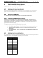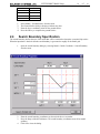
1
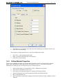
2D Slope Stability Modeling Software
Tutorial Manual
Date Last Edited: November 24, 2004
Written by:
Murray Fredlund, Ph.D.
Gilson Gitirana, Ph.D.
Robert Thode, B.Sc.G.E.
Edited by:
Murray Fredlund, Ph.D.
SoilVision Systems Ltd.
Saskatoon, Saskatchewan, Canada
Software License
The software described in this manual is furnished under a license agreement. The software may be used or
copied only in accordance with the terms of the agreement.
Software Support
Support for the software is furnished under the terms of a support agreement.
Copyright
Information contained within this User’s Manual is copyrighted and all rights are reserved by SoilVision
Systems Ltd. The SVFLUX software is a proprietary product and trade secret of SoilVision Systems. The
User’s Manual may be reproduced or copied in whole or in part by the software licensee for use with
running the software. The User’s Manual may not be reproduced or copied in any form or by any means
for the purpose of selling the copies.
Disclaimer of Warranty
SoilVision Systems Ltd. reserves the right to make periodic modifications of this product without obligation
to notify any person of such revision. SoilVision does not guarantee, warrant, or make any representation
regarding the use of, or the results of, the programs in terms of correctness, accuracy, reliability, currentness,
or otherwise; the user is expected to make the final evaluation in the context of his (her) own problems.
Trademarks
Windows™ is a registered trademark of Microsoft Corporation.
SoilVision® is a registered trademark of SoilVision Systems Ltd.
SVFLUX ™ is a trademark of SoilVision Systems Ltd.
CHEMFLUX ™ is a trademark of SoilVision Systems Ltd.
SVSOLID ™ is a trademark of SoilVision Systems Ltd.
SVHEAT ™ is a trademark of SoilVision Systems Ltd.
ACUMESH ™ is a trademark of SoilVision Systems Ltd.
FlexPDE® is a registered trademark of PDE Solutions Inc.
Surfer® is a registered trademark of Golden Software Inc.
Slicer Dicer® is a registered trademark of Visualogic Inc.
Copyright © 2005
by
SoilVision Systems Ltd.
Saskatoon, Saskatchewan, Canada
ALL RIGHTS RESERVED
Printed in Canada
Table of Contents
3
of
1 Tutorial Example Model
...................................................................................................................................
1.1 Adding
a Project
...................................................................................................................................
1.2 Adding
a Model
...................................................................................................................................
1.3 Opening
the Model
...................................................................................................................................
1.4 Defining
the Model
1.4.1 ...................................................................................................................................
Specify Settings
1.4.2 ...................................................................................................................................
Setting the Workspace
1.4.3 ...................................................................................................................................
Define Material Properties
1.4.4 ...................................................................................................................................
Adding Regions
1.4.5 ...................................................................................................................................
Defining Region Geometry Shapes
1.4.6...................................................................................................................................
Specify Boundary Conditions
...................................................................................................................................
1.5 Specifying
the Water Table
...................................................................................................................................
1.6 Specify
Plots
...................................................................................................................................
1.7 Specify
Output Files
...................................................................................................................................
1.8 Analyze
2 SVDYNAMIC Model Setup
...................................................................................................................................
2.1 Adding
a Project and Model
...................................................................................................................................
2.2 Defining
the Model
2.2.1...................................................................................................................................
Importing Geometry from SVSOLID
...................................................................................................................................
2.3 Adding
the Ground Surface
...................................................................................................................................
2.4 Search
Boundary Specification
...................................................................................................................................
2.5 Analyze
the Slope
...................................................................................................................................
2.6 Results
3 References
16
4
5
6
6
6
6
7
8
9
9
10
11
12
12
12
13
13
13
13
13
14
15
15
16
4
Tutorial Example Model
1
of
16
Tutorial Example Model
The following example will introduce the operation and features of SVDYNAMIC and will provide
instructions on how to setup a model of a simple till slope with a weak clay seam. A water table is present as
well as a proposed roadbed to which a load is applied. The purpose of this model is to determine the slip
surface for the present conditions and the resulting factor of safety for the slip surface. The model dimensions
and soil properties are provided below.
SVDYNAMIC Project Name: Tutorial
Model Name: Tutorial1
SVSOLID Project Name: Tutorial
Model Name: Tutorial_SVDynamic
Region Geometry
Ground
Seam
Water Table
X
Y
X
Y
X
Y
0
0
0
25
0
36
100
0
68
25
58
34
100
20
64
28
85
20
0
28
80
22
78
24
Tutorial Example Model
72.8
22.4
68
25
64
28
62.4
30
57.2
35
52
37
46.8
40
41.6
41
36.4
50
31.2
50
26
50
20.8
48
15.6
50
10.4
56
0
58
5
of
16
Soil Properties
Soil 1:
Till
Young’s Modulus, E = 10000 kPa
Poisson’s Ratio, n = 0.4
Initial Void Ratio, eo = 0.3
Vertical Body Load, gy = -21 kN/m3
Cohesion, c = 25 kPa
Friction Angle, f = 30o
Soil 2:
Weak Clay
Young’s Modulus, E = 3000 kPa
Poisson’s Ratio, n = 0.35
Initial Void Ratio, eo = 0.3
Vertical Body Load, gy = -18 kN/m3
Cohesion, c = 0 kPa
Friction Angle, f = 10o
1.1
Adding a Project
The first step in defining a model is to decide the project under which the model is going to be organized. If
the project is not yet included you must add the project before proceeding with the model. In this case, the
model is placed under a project called Tutorial.
In order to add the project follow these steps:
1.
2.
3.
4.
Access the SVOffice 2006 Manager dialog.
Click New in the upper right of the Projects dialog.
The Create New Project dialog is opened along with a prompt asking for a new Project Name.
Type “Tutorial” as the new Project Name and press OK.
The Project Properties dialog is where information specific to each project is stored. This will include the
Tutorial Example Model
6
of
16
Project Name, Project Folder, and Project Notes information.
The Project Name is the only required information needed to define a project. The rest of the
fields are optional.
The dialog is opened ready to accept information.
It should be noted that once the project is defined it would be identified by the Project Name throughout the
rest of the program. Also, SVSOLID does not allow you to specify two projects with the same Project Name.
5.
6.
1.2
Fill out the dialog with the desired information.
To exit this dialog and return to SVOffice 2006 Manager, click OK. The project information is
automatically saved upon entry.
Adding a Model
Once a project has been created any number of models may be stored in Corresponding Models Under The
Project.
When the SVOffice 2006 Manager dialog is opened there will be a list of the projects that have been defined.
In this case there is only the Tutorial project. To add a model:
1.
2.
3.
4.
5.
1.3
Click on "New" in Corresponding Models Under The Project.
Enter Tutorial_SVDynamic in the Model Name box.
This example will be modeled in two-dimensions and is steady-state so we must select 2D for
System and Steady-State for Type.
Click the OK button to save the model and close the New Model dialog.
The new model will automatically added to Corresponding Models Under The Project.
Opening the Model
If the model was just added it will appear in the Corresponding Models Under The Project. Follow these steps
to open it in the workspace:
1.
2.
3.
1.4
Navigate back to the model via the Tutorial - 2D item.
Select Tutorial_SVDynamic.
The model may opened by clicking the OK button or by double clicking on the Model Name in
the tree. The model will now be opened in the workspace.
Defining the Model
The following section provides instructions on how to begin defining the model in the workspace.
1.4.1
Specify Settings
The first step in defining the model is to specify the settings that will be used for the model. To open the
Settings dialog select Model > Settings in the workspace menu.
The Settings dialog will contain information about the current model System, Analysis, Units, Initial
Conditions Settings, and more. The data for the model is in metric so the units will remain metric.
Tutorial Example Model
7
of
16
Options must be selected here in order to specify a water table as the initial pore-water pressure conditions.
Drawing of the water table is explained later in this tutorial.
1.
2.
3.
4.
5.
1.4.2
Select Consider PWP as the Analysis option.
Click OK to close the dialog.
Select Model > Initial Conditions > Settings from the menu. Select the Initial Pore Water
Pressure tab.
Select Draw Water Table as the Initial PWP Option.
Click OK to close the dialog.
Setting the Workspace
Before entering any model geometry it is best to set the World Coordinate System to ensure that the model
will fit in the drawing space.
1.
2.
Access the View Settings dialog by selecting View > Settings.
Enter the View Coordinates shown below into the Scale tab for the X and Y axis.
3.
4.
Enter the view coordinates as shown above.
Also set the CAD Window (drawing space) coordinates.
Tutorial Example Model
5.
6.
8
of
16
Select Format > Axis from the menu. Enter the values shown above for both the X and Y axis.
Click OK to close the dialog.
The workspace grid spacing needs to be set to aid in defining region shapes.
1.
2.
3.
1.4.3
Select View > Grid Spacing from the menu.
Enter 1 for both the horizontal and vertical spacing.
Click OK to close the dialog.
Define Material Properties
The next step in defining the model is to enter the material properties for the 2 soils that will be used in the
model. A till is defined for the slope and the seam will consist of a clay soil. This section will provide
instructions on creating the clay soil. Repeat the process to add the other soil.
1.
2.
3.
4.
5.
6.
Open the Soils dialog by selecting Model > Soils > Manager from the menu.
Click the New Soil button to create a soil.
Select the new soil and click Properties to open the Soil Properties dialog.
Enter the information above into the appropriate fields on the Description tab.
Move to the Parameters tab.
Refer to the data provided at the beginning of this tutorial. Enter the Young’s Modulus value of
3000 kPa.
Tutorial Example Model
7.
8.
9.
10.
11.
12.
13.
14.
15.
9
of
16
Enter the Poisson’s Ratio value of 0.35.
Enter the Initial Void Ratio value of 0.3.
Move to the Body Load tab.
Enter the X-Axis Body Load as 0 kN/m3.
Enter the Y-Axis Body Load as –18 kN/m3.
Move to the Shear Strength tab.
Enter the Cohesion as 0 kPa.
Enter the Friction Angle as 10o.
Repeat these steps to create the till soil.
The negative sign for the body load indicates that the vertical body load will act down.
1.4.4
Adding Regions
A region in SVSOLID is the basic building block for a model. A region represents both a physical portion of
soil being modeled and a visualization area in the SVSOLID CAD workspace. A region will have a set of
geometric shapes that define its soil boundaries. Also, other modeling objects including features, water tables,
text, and line art are defined on any given region.
This model will be divided into three regions, which are named Slope, Clay Seam, and Water Table. The first
2 regions will have one of the soils just defined specified as its soil properties. The third region will be used
just to draw the water table. To add the necessary regions follow these steps:
1.
2.
3.
4.
5.
6.
7.
8.
9.
1.4.5
Open the regions dialog by selecting Model > Geometry > Regions from the menu.
Change the first region name from Region 1 to Slope. Highlight the name and type new text.
Select the Soil Index from the drop-down corresponding to the till.
Press the New button to add a second region.
Change the name of the second region to Clay Seam.
Select the clay soil for the Clay Seam region.
Click New to add the third region.
Name it Water Table.
Click OK to close the dialog.
Defining Region Geometry Shapes
The shapes that define each soil region will now be created. Note that when drawing geometry shapes the
region that is current in the region selector is the region the geometry will be added to. The Region Selector is
at the top of the workspace.
· Define the Ground
To draw the slope the instructions below explain the use of the Region Properties dialog to create the
core shape.
1.
2.
3.
4.
5.
6.
Ensure that “Slope” is current in the region selector.
Select Model > Geometry > Region Properties from the menu.
The Shape 1 tab will open.
Type 0 into the X column and 0 into the Y column.
Type 100 into the X column and 0 into the Y column.
Refer to the geometry table at the beginning of this tutorial at enter the remaining points.
Tutorial Example Model
10
of
16
· Define the Clay Seam
To draw the seam the instructions below explain the use of the mouse to create the core shape.
1.
2.
3.
4.
5.
6.
7.
8.
9.
Ensure the “Clay Seam” region is current in the region selector.
Select Draw > Model Geometry > Polygon Region from the menu.
The cursor will now be changed to cross hairs.
Move the cursor near (0,25) in the drawing space. You can view the coordinates of the current
position the mouse is at in the status bar.
When the cursor is near the point, right click. This will cause the cursor to snap to the point
(The SNAP and GRID options in the status bar must both be bold).
To select the point as part of the shape left click on the point.
Now move the cursor near (68,25). Right click to snap the cursor to the exact point and then
left click on the point. A line is now drawn from (0,25) to (68,25).
Refer to the geometry table at the beginning of this tutorial and add the remaining points.
To add the last point, move the cursor near the point (0,28) and right click snapping the cursor
to the point. Double click on the point to finish the shape. A line is now drawn from (64,28)
to (0,28) and the shape is automatically finished by SVSOLID by drawing a line from (0,28)
back to the start point, (0,25).
Select a shape with the mouse and select Edit > Delete from the menu if a mistake was made
entering the coordinate points for a shape. This will remove the entire shape from the region. To
edit the shape use the Region Properties dialog.
At times it may be tricky to snap to a grid point that is near a line defined for a region. Turn the
object snap off by clicking on “OSNAP” in the status bar to alleviate this problem.
1.4.6
Specify Boundary Conditions
Now that all of the regions and the model geometry have been successfully defined, the next step is to specify
the boundary conditions. A load expression will be defined on the roadway location on the slope region with
the sides being fixed in the X-direction. At the base the region will be fixed in both the X and Y directions.
The Clay Seam region is internal to the Slope region and will not need to be altered. The steps for specifying
the boundary conditions are thus:
1.
2.
3.
4.
5.
6.
7.
8.
9.
10.
11.
12.
13.
14.
Select the “Slope” region in the drawing space.
From the menu select Model > Boundaries > Boundary Conditions. The boundary conditions
dialog will open.
Select the point (0,0) from the list on the Segment tab.
From the X Boundary Condition drop down select a Fixed boundary condition.
From the Y Boundary Condition drop down select a Fixed boundary condition.
Select the point (100,0) from the list.
From the X Boundary Condition drop down select a Continue boundary condition.
From the Y Boundary Condition drop down select a Free boundary condition.
Select the point (100,20) from the list.
From the X Boundary Condition drop down select a Free boundary condition.
Select the point (36.4,50) from the list.
From the Y Boundary Condition drop down select a Load Expression boundary condition.
This will cause the Load Expression box to be enabled.
In the Expression box enter a load of -1000.
Select the point (26,50) from the list.
Tutorial Example Model
11
of
16
15. From the Y Boundary Condition drop down select a Free boundary condition.
16. For the last point, select Fixed as the X Boundary Condition.
17. Click the OK button to close the dialog.
The Free Y boundary condition for the point (100,0) becomes the boundary condition for the
following line segments that have a Continue boundary condition until a new boundary
condition is specified. By specifying a Load Expression condition at point (36.4,50) the
Continue is turned off.
Boundary Condition Summary
X
Y
0
0
X Boundary Condition Y Boundary Condition
Fixed
Fixed
100
0
Continue
Free
100
20
Free
Continue
85
20
Continue
Continue
80
22
Continue
Continue
78
24
Continue
Continue
72.8
22.4
Continue
Continue
68
25
Continue
Continue
64
28
Continue
Continue
62.4
30
Continue
Continue
57.2
35
Continue
Continue
52
37
Continue
Continue
46.8
40
Continue
Continue
41.6
41
Continue
Continue
36.4
50
Continue
Load Expression = -1000
31.2
50
Continue
Continue
26
50
Continue
Free
20.8
48
Continue
Continue
15.6
50
Continue
Continue
10.4
56
Continue
Continue
0
58
Fixed
Continue
1.5
Specifying the Water Table
A water table will be drawn across the model to indicate the initial pore-water pressure conditions. The
pore-water pressure equals 0 at the water table elevation and is hydrostatic in the remainder of the model.
1.
2.
3.
4.
Select Draw < Initial Water Table from the menu.
The Water Table dialog will open. Click the Draw button.
With the mouse click on the point (0,36).
To finish the Water Table double-click on the point (58,34). A dashed-dot line is drawn across
the model.
Tutorial Example Model
1.6
12
of
16
Specify Plots
There are many plot types that can be specified to visualize the results of the model. A vertical stress contour
plot will be generated for this example.
1.
2.
3.
4.
5.
6.
7.
1.7
Open the Plot Manager dialog by selecting Model > Plot Manager from the menu.
The toolbar at the bottom left of the dialog contains a button for each plot type. Click on the
Contour button to begin adding the first contour plot. The Plot Properties dialog will open.
Enter the title Vertical Stress.
Select sy as the variable to plot from the drop-down.
Select the Output Options tab and select the PLOT output option.
Click OK to close the dialog and add the plot to the list.
Click OK to close the Plot Manager and return to the workspace.
Specify Output Files
There are 4 output file types that can be specified to export the results of the model. A pore-water pressure
table file is required for the SVDYNAMIC analysis. A stress table file will be generated automatically as long
as the required soil properties are provided. The file will be called:
Tutorial_Tutorial_SVDynamic_SVDynamicData.tbl.
1.
2.
3.
4.
5.
6.
7.
8.
1.8
Open the Output Manager dialog by selecting Model > Reporting > Output Manager from the
menu.
The toolbar at the bottom left of the dialog contains a button for each output file type. Click on
the Table button to begin adding the output file. The Output File Properties dialog will open.
Enter the title pwp.
Select all the variable uw in the variable list.
Press the Add Selection button.
Check the Write File box.
Click OK to close the dialog and add the output file to the list.
Click OK to close the Output Manager and return to the workspace.
Analyze
The next step is to analyze the model. Click the Analyze button located in the toolbar. This action will write
the descriptor file and open the SVSOLID solver. The solver will automatically begin solving the model.
Once the solver has completed analyzing the model it will generate the stress state .TBL that is called
Tutorial_Tutorial_SVDynamic_SVDynamicData.tbl. The default format for this file is
ProjectName_ModelName_SVDynamicData.tbl. The specified pwp.tbl file will also be created.
SVDYNAMIC Model Setup
2
13
of
16
SVDYNAMIC Model Setup
After the model has been created and solved in SVSOLID, the model data can be imported into
SVDYNAMIC and the slope stability setup can be done.
2.1
Adding a Project and Model
Projects and models in SVDYNAMIC are created the same way as in SVSOLID. Refer to the SVSOLID
portion of this Tutorial Manual and create the Project Name: Tutorial and the Model Name: Tutorial1.
2.2
Defining the Model
The following section provides instructions on how to set up the model in SVDYNAMIC.
2.2.1
Importing Geometry from SVSOLID
Geometry for the SVDYNAMIC model is imported from an SVSOLID model. The geometry must be
imported before any other modeling operations are available. The import includes regions, region shapes,
world coordinate system settings, and water tables. The units for the SVDYNAMIC model are set to the
SVSOLID model units during import.
To import the geometry from the SVSOLID model previously created:
1.
2.
3.
4.
2.3
Select Model > Import Geometry > From Existing Model from the menu to open the above
Import SVSolid Geometry dialog.
The Import Geometry dialog will open. Specify the Tutorial Project the geometry will be
imported from.
Select the Model Name: Tutorial_SVDynamic from Corresponding Models under the project.
Press Import.
Adding the Ground Surface
The Ground Surface is a necessary component of the SVDYNAMIC analysis and should correspond to the top
of the model geometry. The following list contains the ground surface points:
X
Y
100
20
85
20
80
22
78
24
72.8
22.4
68
25
64
28
62.4
30
57.2
35
52
37
46.8
40
41.6
41
36.4
50
31.2
50
SVDYNAMIC Model Setup
1.
2.
3.
4.
2.4
26
50
20.8
48
15.6
50
10.4
56
0
58
14
of
16
Select Model > Ground Surface from the menu.
The Ground Surface dialog is displayed without any data.
Enter the above coordinate points for the ground surface.
Press the OK key to complete the ground surface.
Search Boundary Specification
The search boundary defines the area of the model that will be examined to determine a potential slip surface.
When the input data is loaded a default search boundary is generated to roughly fit the model grid.
1.
Open the search boundary dialog by selecting Model > Initial Conditions > Search Boundary
from the menu.
2.
3.
Enter the search boundary coordinates as shown in the above screenshot.
Press the Snap to Model Grid button. The search boundary coordinates must fall on model
gridlines.
Click OK to close the dialog.
4.
SVDYNAMIC Model Setup
15
of
16
See the SVDYNAMIC User’s Manual for all the requirements of the search boundary.
2.5
Analyze the Slope
The model setup is now complete. From the menu select Solve > Analyze or press the Analyze button in the
toolbar. SVDYNAMIC will begin solving the model and will open the Analysis Message Window.
2.6
Results
After the SVDYNAMIC solver has analyzed a model it will display the final factor of safety and analysis time
in the Message Window. The resulting Slip Surface will also be drawn in the workspace and the factor of
safety for the slip surface will be shown in the upper right portion of the workspace.
The factor of safety for the slip surface of this slope under the defined conditions is 0.77.
Once an analysis has been completed and the slip surface generated distance graphs can be plotted. A distance
graph is an input or output variable vs. distance along the slip surface. Select Model > Plots to open the
Distance Graph dialog.
References
3
16
of
16
References
D. G. Fredlund and H. Rahardjo, 1993. Soil Mechanics for Unsaturated Soils. John Wiley & Sons, New York
Ha T. V. Pham, 2002. Slope Stability Analysis Using Dynamic Programming Method With A Finite Element
Stress Analysis. University of Saskatchewan, Canada
Fredlund, D.G., and Gitrana Jr, G.F.N. 2003. Analysis Of Transient Embankment Stability Using The
th
Dynamic Programming Method. Proceedings of the 56 Canadian Geotechnical Conference,
Winnipeg, Canada. Sept.29 to Oct 1, Vol. 1, pp. 807 to 814.