Download Brief User Guide for Program CARE-3: Analyzing Continuous

September, 2003
Brief User Guide for Program CARE-3:
Analyzing Continuous-Time Capture-Recapture Data
Wen-Han Hwang and Anne Chao
Program CARE-3 (for CApture-REcapture) is written in GAUSS language and the
program calculates population size estimates for various closed continuous-time
capture-recapture models with/without covariates. Relevant covariates such as
environmental variables or individuals characteristics can be incorporated into the
models to assess the effect of each covariate on the capture probabilities.
Program CARE-3 can be downloaded from Anne Chao’s website at
http://chao.stat.nthu.edu.tw/softwareCE.html.
The source files along with
illustrative data sets will be stored automatically in a specified directory in your
computer.
You do not need to purchase GAUSS software to run this program. A working
environment of Gauss is provided by the following procedures: First doubly click the
downloaded file “care-3.exe” to unzip all files to the specified folder. Then doubly
click the “GRTM.exe” to unzip all files of the “Gauss Run-Time Module” (GRTM),
which is GUASS free-ware for non-commercial redistribution. Then doubly click
the “setup.exe” to install the GRTM. (The GRTM allows licensee to redistribute
licensee’s compiled GAUSS programs free of charge to other users who do not have
GAUSS so long as licensee’s GAUSS program is distributed free of charge.) Then
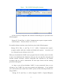
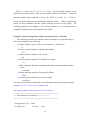
restart your computer after completing the installation of GRTM. As the computer
restarts in Window interface, doubly click the icon “GSRUN50” on the desktop of
your computer to initialize Gauss Run-Time Module and then the interface is shown
below.
-1-
Figure. The GAUSS Working Environment
All the necessary background and estimation methodologies are provided in the
following paper:
Hwang, W. H. and Chao, A. (2002). Continuous-time capture-recapture models
with covariates. Statistica Sinica 12, 1115-1131.
For models without covariates, more details are given in the following paper:
Hwang, W-H, Chao, A. and Yip, P. S. F. (2002). Continuous-time capturerecapture models with time variation and behavioral response. Australian and
New Zealand Journal of Statistics 44, 41-54.
When you download the GAUSS source program from the website, please note that
we have also distributed four illustrative data sets (the two data files simeg.dat and
coul.dat contain covariates, whereas simeg2.dat and coul2.dat do not include
covariates) that are used to demonstrate the data input format and the running
procedure in this guide.
As long as you will not distribute CARE-3 in any commercial form, you are
welcome to use CARE-3 for your own research and applications.
If you publish
your work based on the results from CARE-3, please use the following reference for
citing CARE-3.
Hwang, W.-H. and Chao, A. (2003) Program CARE-3: CApture-REcapture
-2-
(Part 3). Program and User's Guide published at http://chao.stat.nthu.edu.tw.
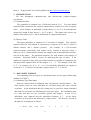
1. INTRODUCTION
We first distinguish continuous-time and discrete-time capture-recapture
experiments:
(1) Continuous-Time:
The population is sampled over a fixed time interval [0, τ ]. For each animal
captured in the experiment, the complete capture history consists of a series of capture
times. As an example, an individual’s capture history (1, 4, 6.5, 8, 9) means that the
animal was caught in time unit of 1, 4, 6.5, 8 and 9. The capture time can be any
number in the interval [0, τ ], but an animal may be captured many times.
(2) Discrete-Time:
The target population is sampled over T occasions or samples. The complete
capture history for each animal is expressed as a sequence of 0’s and 1’s, where 0
denotes absence and 1 denotes presence. For example, in a five-occasion
capture-recapture experiment, each animal can be counted at most five times; a
history (0 1 0 0 1) means that the animal was caught in the second and fifth occasions,
but not in the others. The maximum frequency for each animal is the number of
occasions. (Program CARE-2 focuses on analyzing this type of data.) If the
number of occasions is large, this type of data can also be regarded as continuous-type
and the possible captures times are the integers 1, 2, ..., T. For example, in the case
of T = 10, a history (0 1 0 0 1 0 1 1 0 1) for which the individual was caught on
occasions 2, 5, 7, 8 and 10 corresponds to capture times 2, 5, 7, 8, and 10.
2.
DATA INPUT FORMAT
Corresponding to the two types of experiments, there are two types of data input
formats for CARE-3:
(1) Continuous Type Data Input:
Data are collected from a continuous-time experiment as described above. The
exact capture times for each individual are recorded along with some relevant
covariates. In the distributed data file (simeg.dat), we provide a simple simulated
data with two covariates for illustrating the necessary input. The termination time
is 2 units and there are two covariates (gender and weight). A total of 161
individuals were captured and the maximum frequency is 7. In the input,
covariates are first given and followed by capture times. The first five records in
the data file are displayed as follows:
0
20.585
0.005
1.098
1.551
0
-3-
0
0
0
0
21.876
0.007
1.604
1.741
0
0
0
0
1
18.579
0.018
0.256
0.365
0.495
0.526
0.624
1.636
1
20.969
0.041
0.171
0.174
0.471
1.860
1.869
0
1
18.538
0.044
0.488
0.539
0.679
1.407
1.733
0
The first column shows the gender (1:male, 0:female); the second column
denotes the weight in gram, and the other columns record the exact capture times.
For example, the first record indicates that a female individual with weight 20.585
grams was caught in time units of 0.005, 1.098 and 1.551. Note that four extra 0’s
must be added to fit our required input. The third record shows that a male
individual with 18.579 grams was caught seven times; no additional 0’s are added
because seven times is the maximum frequency. The fifth record means that a male
with weight 18.538 grams was caught six times in time units of 0.044, 0.488, 0.539,
0.679, 1.407 and 1.733. A zero is added in the last column to fit the required input.
(2) Discrete Type Data Input:
Data are collected from a discrete-time experiment and are arranged in the usual
“individual capture history” as described in CARE-2 for discrete-time data analysis.
In the distributed file coul.dat, we store the data for a ten-occasion house mouse
collected by Coulombe and discussed in Section 4 of Hwang and Chao (2002). The
reader is referred to the above paper for further details. There were 171 animals
caught with two covariates: gender and age (adult and non-adult). For each record,
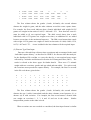
the covariates must precede the capture history. For example, the first five records
in the file coul.dat are given below:
0
1
1
1
1
1
0
0
0
0
0
1
1
1
1
1
1
1
0
0
0
0
1
0
0
1
1
0
1
0
0
1
1
0
0
0
1
0
1
1
0
0
0
0
1
0
1
1
1
1
1
0
0
0
1
0
0
1
0
0
The first column shows the gender (1:male, 0:female); the second column
denotes the age (1:adult, 0:non-adult) and the other columns record presence (1) or
absence (0) in each occasion. For example, the first record means a female adult
was caught on occasions 1, 2, 3, 4 and 10 and not in the others. Similar
interpretation pertains to the other records.
When covariates are not recorded or considered, the data input format is similar
-4-
except that there are no columns for covariates. In the distributed data files,
simeg2.dat and coul2.dat, contain identical capture records as those in simeg.dat and
coul.dat but the covariates are dropped.
Remark: The data file must be saved as an askii file. If your data were
originally processed by EXCEL, please re-save it as .prn file (using blank as
separation of numbers).
CARE-3 will not work if you re-save it as .txt (using tab as
separation) file.
3. MODELS AND ESTIMATES FEATURED IN CARE-3
Assume there are N individuals, indexed by 1, 2, …, N. Also assume that the
experiment period is relatively short so that the population size remains fixed in the
study period. Suppose that the experiment terminates at the time τ and Ni(t) denotes
the number of times the ith animal has been caught in [0, t]. Each {Ni(t); 0 ≤ t ≤ τ}
is a continuous-time counting process with intensity λi(t). The intensity for the ith
animal, λi (t ) is λi (t ) dt = P{dN i (t ) = 1 Ft − } , where Ft is the capture history
generated by {N1 (u ), N 2 (u ),..., Nν (u ); 0 ≤ u ≤ t} .
Let the associated covariates for
the ith individual be Z i = ( Z i1 , Z i 2 ,..., Z i p )′ , where p denotes the number of covariates.
In program CARE-3, we only handle the estimation procedure for time-independent
covariates because an experiment’s duration is usually short for a closed model as a
matter of practice.
Let λ0 (t ) be any arbitrary non-negative time-varying function defined in [0, τ].
The covariates are used to model individual heterogeneity. Let β = ( β1 , β 2 , ..., β p )′
be a vector of unknown regression coefficients. We use λ0(t), exp( β ′ Z i ) and φ to
model respectively the time, heterogeneity and the behavioural response effects.
Thus a multiplicative type of model Mtbh is
 λ (t ) exp( β ′ Z i ) until first capture,
λi (t ) =  0
φ λ0 (t ) exp( β ′ Z i ) for any recapture.
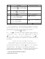
The continuous-time models featured in CARE-3 are summarized in Table 1.
Table 1. Continuous-Time Models Featured in CARE-3
-5-
Model
Assumption
Restriction in model Mtbh
Mtbh
 λ (t ) exp( β ′ Z i ) until first capture,
λi (t ) =  0
φ λ0 (t ) exp( β ′ Z i ) for any recapture.
Mbh
 λ exp( β ′ Z i ) until first capture,
λi (t ) = 
φ λ exp( β ′ Z i ) for any recapture.
Mth
λi (t ) = λ0 (t ) exp( β ′ Z i )
Mtb
 λ (t ) until first capture,
λi (t ) =  0
φ λ0 (t ) for any recapture.
Mb
 λ until first capture,
λi (t ) = 
φ λ for any recapture.
i.e. β = 0, λ0 (t ) ≡ λ in model Mtbh
Mt
λi (t ) = λ0 (t )
i.e. set φ = 1, β = 0 in model Mtbh
i.e. set λ0 (t ) ≡ λ in model Mtbh
i.e. set φ = 1 in model Mtbh
i.e. β = 0 in model Mtbh
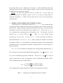
Let φ = exp(α) and Xi (t) = I [the ith animal has been captured in (0, t)] denotes
the prior capture history, where I [.] is the usual indicator function. For the most
general model Mtbh, the intensity of the ith individual can be rewritten as
λi (t ) = λ0 (t )exp( β ′ Z i + αX i (t )) .
Let γi = exp( β ′Z i ) and denote the baseline cumulative intensity function by
t
Λt = ∫ 0 λ0 (u )du , t ∈ [0, τ ] .
Also, let the conditional MLE be denoted as
( βˆ ,φˆ, Λˆτ ) = ( βˆ1 , βˆ2 , ..., βˆ p , φˆ , Λˆτ ), then we subsequently get γˆi = exp( βˆ ′ Z i ) .
The proposed Horvitz-Thompson type of population size estimator in Hwang and
Chao (2002) is
Mτ
νˆ = ∑ I (δ i = 1) /[1 − exp( −γˆi Λˆτ )] = ∑ 1 /[1 − exp( −γˆi Λˆτ )] .
δ i =1
i =1
Program CARE-3 calculates the above population size estimate and its s.e. as
well as the regression coefficients, i.e., estimate of β = ( β1 , β 2 , ..., β p )′ for the above
four models in Table 1. The estimated s.e. for all estimates are obtained by an
asymptotic method except for model Mtbh. For model Mtbh, Hwang and Chao (2002)
suggested a bootstrap procedure to obtain s.e. See the above paper for details.
4. RUNNING PROCEDURES BY EXAMPLES
4.1 Models With Covariates
-6-
Example 1: (Continuous Type Data; Data is stored in the file c:\simeg.dat)
We describe the procedures for analyzing the data in the file simeg.dat. All
procedures must be executed in a GAUSS environment.
(1) Provoke GAUSS environment either by doubly clicking GSRUN50 on your
desktop as described earlier or by clicking the executable file GSRUN.exe stored
in the directory GSRUN50.
(2) Click “File” on the top menu of GAUSS and subsequently click “Run Program”
and select the program CARE-3.gcg which is stored in a pre-specified working
directory (The default is c:\program files\CARE-3\).
It prompts you
subsequently the following input steps:
(3) Then proceed the following steps:
(a) Please input the type of data (1 for continuous, 2 for discrete)
?1
(b) Please input the number of distinct individuals:
? 161
(c) Please input the maximum frequency:
?7
(d) Please input the end time of study period:
?2
(e) Please input the number of individual covariates:
?2
(f) Please input the filename containing individual covariates and the capture
times
c:\simeg.dat
(g) Please input the number of bootstrap replications for obtaining s.e. under
model Mtbh:
? 200
(Note: This step specifies the number of bootstrap replications for calculating
variance estimator for model(tbh). A suggested number of bootstrap
replications is 500. Here we use 200 is just for demonstration. You may
specify a larger number, but it will take longer execution time)
(h) Please input the filename to save the output:
c:\test.out
Then wait for a while for executing the program, the output will be shown in the
output window in GAUSS and also will be saved in the designated file. The above
specification corresponds to the following setting in the source program:
-7-
datatype=1, r=161, c=7, p=2, tau=2, and nb=200.
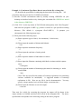
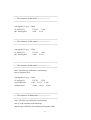
The results in output window are shown below (also saved in c:\test.out):
===========================================
=== The estimates of Mt model ============
===========================================
converged?('0'=yes) 0.000
N^ and se(N^)
185.560
6.418
===========================================
=== The estimates of Mb model ============
===========================================
converged?('0'=yes) 0.000
N^ and se(N^)
212.078 21.194
phi^ and se(phi^)
1.514 0.324
===========================================
=== The estimates of Mtb model ============
===========================================
converged?('0'=yes) 0.000
N^ and se(N^)
183.657 12.535
phi^ and se(phi^)
0.960 0.236
===========================================
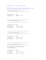
=== The estimates of Mth model ============
===========================================
Note: The first reg coefficient is an intercept
beta_0=ln(landa_tau).
converged?('0'=yes) 0.000
N^ and se(N^)
197.201 9.463
reg coefficients
1.690 0.643 -0.072
-8-
standard error
0.689
0.144
0.034
===========================================
=== The estimates of Mbh model ============
===========================================
Note: The first reg coefficient is an intercept
beta_0 is the estimate of the intercept;
and the 1ast coefficient is the behavioral response effect
theta_{p+2}=ln(phi)
converged?('0'=yes) 0.000
N^ and se(N^)
239.685 30.749
reg coefficients
0.564 0.693 -0.073 0.495
standard error
0.745 0.151 0.036 0.223
===========================================
=== The estimates of Mtbh model ===========
===========================================
Note: The first reg coefficient is an intercept
theta_0=ln(landa_tau);
and the 1ast coefficient is the behavioral response effect
theta_{p+2}=ln(phi)
converged?('0'=yes) 0.000
N^ and se(N^)
205.824 31.970
reg coefficients
1.582 0.658 -0.072 0.127
standard error
0.694 0.154 0.033 0.323
To help the user interpret the results, we discussed the numerical outputs for two
models Mtbh and Mth. Let Z1 denote the covariate gender and let Z2 denote the
covariate weight. The intensity function for the most general model Mtbh was
assumed to be λi (t ) = λ0 (t ) exp( β1Z i1 + β 2 Z i 2 + αX i (t )) , where Z i1 = I [the ith
individual is a male], Z i 2 = weight, and Xi (t) = I [the ith individual has been captured
in (0, t)]. The parameter estimates under model Mtbh are β$1 = 0.658 (s.e. 0.15), β$2
-9-
= -0.072 (s.e. 0.032) and αˆ = 0.127 (s.e. 0.316). The behavioral response is not
significantly different from 0, thus a proper model would be model Mth. Based on
the above output, under model Mth, we have β$1 = 0.643 (s.e. 0.144), β$2 = -0.072 (s.e.
0.034) and both coefficients are significantly different from 0. Hence it implies that
males are more catchable and the capture intensity decreases with weight. The
resulting population size estimate is 197 with an estimated s.e. of 9.46 based on an
asymptotic formula given in Hwang and Chao (2002).
Example 2: (Discrete Type Data; Data is stored in the file c:\coul.dat)
The running procedures are similar to those in Example 1 except that Steps (c)
and (d) are changed to the following:
(a) Please input the type of data (1 for continuous, 2 for discrete)
?2
(b) Please input the number of distinct individuals:
? 171
(c) Please input the number of occasions:
? 10
(d) Please input the number of individual covariates:
?2
(e) Please input the filename containing individual covariates and the capture
times
c:\coul.dat
(f) Please input the number of bootstrap for Mtbh:
? 200
(g) Please input the filename to save the output:
c:\test2.out
The above specification corresponds to the following setting in the source program:
datatype=2, r=171, c=tau=10, p=2, and nb=200.
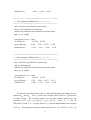
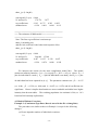
The output is shown below (also saved in c:\test2.out):
===========================================
=== The estimates of Mt model ============
===========================================
converged?('0'=yes) 0.000
N^ and se(N^)
172.198
1.931
- 10 -
===========================================
=== The estimates of Mb model ============
===========================================
converged?('0'=yes) 0.000
N^ and se(N^)
176.833 3.388
phi^ and se(phi^)
0.981 0.110
===========================================
=== The estimates of Mtb model ============
===========================================
converged?('0'=yes) 0.000
N^ and se(N^)
172.195 1.681
phi^ and se(phi^)
1.000 0.139
===========================================
=== The estimates of Mth model ============
===========================================
Note: The first reg coefficient is an intercept
beta_0=ln(landa_tau).
converged?('0'=yes) 0.000
N^ and se(N^)
179.221 3.259
reg coefficients
1.091 -0.175 0.293
standard error
0.089 0.091 0.094
===========================================
=== The estimates of Mbh model ============
===========================================
Note: The first reg coefficient is an intercept
beta_0 is the estimate of the intercept;
and the 1ast coefficient is the behavioral response effect
- 11 -
theta_{p+2}=ln(phi)
converged?('0'=yes) 0.000
N^ and se(N^)
178.776 3.877
reg coefficients
-1.193 -0.175 0.293 -0.022
standard error
0.128 0.091 0.094 0.113
===========================================
=== The estimates of Mtbh model ===========
===========================================
Note: The first reg coefficient is an intercept
theta_0=ln(landa_tau);
and the 1ast coefficent is the behavioral response effect
theta_{p+2}=ln(phi)
converged?('0'=yes) 0.000
N^ and se(N^)
206.009 15.340
reg coefficients
0.497 -0.155 0.329 0.687
standard error
0.226 0.074 0.080 0.258
We interpret the results for the most complicated model Mtbh. The model
assume an intensity function λi (t ) = λ0 (t ) exp( β 1 Z i1 + β 2 Z i 2 + αX i (t )) where Z i1 = I
[the ith individual is a male], Z i 2 = I [the ith individual is an adult], and Xi (t) = I [the
ith individual has been captured in (0, t)]. The parameter estimates are β$1 = − 0.155
(s.e. 0.08), β$2 = 0.329 (s.e. 0.08) and αˆ = 0.687 (s.e. 0.253) and all coefficients are
significant. Hence it implies that females are more catchable and adults have higher
intensity than do non-adults. The resulting population size estimate is 206 (s.e. 14.2
based on 200 bootstrap replications).
4.2 Models Without Covariates
Example 3: (Continuous Type Data; Data is stored in the file c:\simeg2.dat)
The procedures are similar to those in Example 1 except for the following
changes:
(e) Please input the number of individual covariates:
?0
- 12 -
(f) Please input the filename containing individual covariates and the capture
times
c:\simeg2.dat
(g) Please input the number of bootstrap replications for obtaining s.e. under
model Mtbh:
?0
(h) Please input the filename to save the output:
c:\test3.out
Then wait for a while for executing the program, the output will be shown in the
output window in GAUSS and also will be saved in the designated file. The above
specification corresponds to the following setting in the source program:
datatype=1, r=161, c=7, p=0, tau=2, and nb=0.
The results in output window are shown below (also saved in c:\test3.out):
===========================================
=== The estimates of Mt model ============
===========================================
converged?('0'=yes) 0.000
N^ and se(N^)
185.560
6.418
===========================================
=== The estimates of Mb model ============
===========================================
converged?('0'=yes) 0.000
N^ and se(N^)
212.078 21.194
phi^ and se(phi^)
1.514 0.324
===========================================
=== The estimates of Mtb model ============
===========================================
- 13 -
converged?('0'=yes) 0.000
N^ and se(N^)
183.657 12.535
phi^ and se(phi^)
0.960 0.236
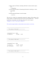
Example 4: (Discrete Type Data; Data is stored in the file c:\coul2.dat)
The procedures are similar to those in Example 2 except for the following
changes:
(d) Please input the number of individual covariates:
?0
(e) Please input the filename containing individual covariates and the capture
times
c:\coul2.dat
(f) Please input the number of bootstrap for Mtbh:
?0
(g) Please input the filename to save the output:
c:\test4.out
The above specification corresponds to the following setting in the source program:
datatype=2, r=171, c=tau=10, p=0, and nb=0.
The output is shown below
===========================================
=== The estimates of Mt model ============
===========================================
converged?('0'=yes) 0.000
N^ and se(N^)
172.198
1.931
===========================================
=== The estimates of Mb model ============
===========================================
converged?('0'=yes) 0.000
N^ and se(N^)
176.833 3.388
phi^ and se(phi^)
0.981 0.110
- 14 -
===========================================
=== The estimates of Mtb model ============
===========================================
converged?('0'=yes) 0.000
N^ and se(N^)
172.195 1.681
phi^ and se(phi^)
1.000 0.139
- 15 -