1
PMLAB
User Guide
Marc Solé
Josep Carmona
13-05-14
2
Contents
1 Introduction
1.1 Motivation . . . . . . . . . . . . . . . .
1.2 Log extraction . . . . . . . . . . . . . .
1.3 Organization of the Package . . . . . . .
1.4 Downloading . . . . . . . . . . . . . . .
1.5 Contributors . . . . . . . . . . . . . . .
1.6 License . . . . . . . . . . . . . . . . . . .
1.7 Installation . . . . . . . . . . . . . . . .
1.7.1 Option 1: virtualized installation
1.7.2 Option 2: source Installation . .
1.8 IPython basics . . . . . . . . . . . . . .
.
.
.
.
.
.
.
.
.
.
.
.
.
.
.
.
.
.
.
.
.
.
.
.
.
.
.
.
.
.
.
.
.
.
.
.
.
.
.
.
.
.
.
.
.
.
.
.
.
.
.
.
.
.
.
.
.
.
.
.
.
.
.
.
.
.
.
.
.
.
.
.
.
.
.
.
.
.
.
.
.
.
.
.
.
.
.
.
.
.
.
.
.
.
.
.
.
.
.
.
.
.
.
.
.
.
.
.
.
.
.
.
.
.
.
.
.
.
.
.
.
.
.
.
.
.
.
.
.
.
.
.
.
.
.
.
.
.
.
.
.
.
.
.
.
.
.
.
.
.
.
.
.
.
.
.
.
.
.
.
.
.
.
.
.
.
.
.
.
.
.
.
.
.
.
.
.
.
.
.
.
.
.
.
.
.
.
.
.
.
.
.
.
.
.
.
.
.
.
.
.
.
.
.
.
.
.
.
.
.
.
.
.
.
.
.
.
.
.
.
.
.
.
.
.
.
.
.
.
.
.
.
.
.
.
.
.
.
.
.
.
.
.
.
.
.
.
.
.
.
.
.
.
.
.
.
.
.
.
.
.
.
.
.
.
.
.
.
.
.
.
.
.
.
.
.
.
.
.
.
5
5
5
6
6
7
7
7
7
7
8
2 Logs
2.1 Plain logs and Enhanced logs . . . .
2.2 Manual modification of logs . . . . .
2.3 Loading/Saving . . . . . . . . . . . .
2.4 Encoders . . . . . . . . . . . . . . .
2.4.1 Default encoders . . . . . . .
2.4.2 Loading and saving encoders
2.4.3 Encoding a log . . . . . . . .
2.5 Projections . . . . . . . . . . . . . .
2.6 Filters . . . . . . . . . . . . . . . . .
2.6.1 Default filters . . . . . . . . .
2.6.2 Filtering . . . . . . . . . . . .
2.7 Clustering . . . . . . . . . . . . . . .
2.8 Noise . . . . . . . . . . . . . . . . . .
.
.
.
.
.
.
.
.
.
.
.
.
.
.
.
.
.
.
.
.
.
.
.
.
.
.
.
.
.
.
.
.
.
.
.
.
.
.
.
.
.
.
.
.
.
.
.
.
.
.
.
.
.
.
.
.
.
.
.
.
.
.
.
.
.
.
.
.
.
.
.
.
.
.
.
.
.
.
.
.
.
.
.
.
.
.
.
.
.
.
.
.
.
.
.
.
.
.
.
.
.
.
.
.
.
.
.
.
.
.
.
.
.
.
.
.
.
.
.
.
.
.
.
.
.
.
.
.
.
.
.
.
.
.
.
.
.
.
.
.
.
.
.
.
.
.
.
.
.
.
.
.
.
.
.
.
.
.
.
.
.
.
.
.
.
.
.
.
.
.
.
.
.
.
.
.
.
.
.
.
.
.
.
.
.
.
.
.
.
.
.
.
.
.
.
.
.
.
.
.
.
.
.
.
.
.
.
.
.
.
.
.
.
.
.
.
.
.
.
.
.
.
.
.
.
.
.
.
.
.
.
.
.
.
.
.
.
.
.
.
.
.
.
.
.
.
.
.
.
.
.
.
.
.
.
.
.
.
.
.
.
.
.
.
.
.
.
.
.
.
.
.
.
.
.
.
.
.
.
.
.
.
.
.
.
.
.
.
.
.
.
.
.
.
.
.
.
.
.
.
.
.
.
.
.
.
.
.
.
.
.
.
.
.
.
.
.
.
.
.
.
.
.
.
.
.
.
.
.
.
.
.
.
.
.
.
.
.
.
.
.
.
.
.
.
.
.
.
.
.
.
.
.
.
.
.
.
.
.
.
.
.
.
.
9
9
9
11
11
11
11
12
12
13
13
13
14
14
. . . . . . . .
. . . . . . . .
. . . . . . . .
. . . . . . . .
. . . . . . . .
in graph tool
.
.
.
.
.
.
.
.
.
.
.
.
.
.
.
.
.
.
.
.
.
.
.
.
.
.
.
.
.
.
.
.
.
.
.
.
.
.
.
.
.
.
.
.
.
.
.
.
.
.
.
.
.
.
.
.
.
.
.
.
.
.
.
.
.
.
.
.
.
.
.
.
.
.
.
.
.
.
.
.
.
.
.
.
.
.
.
.
.
.
.
.
.
.
.
.
.
.
.
.
.
.
.
.
.
.
.
.
.
.
.
.
.
.
.
.
.
.
.
.
.
.
.
.
.
.
.
.
.
.
.
.
.
.
.
.
.
.
15
15
15
15
16
16
17
3 Transition Systems
3.1 Obtainig a TS from a log . . . . .
3.2 Loading/Saving . . . . . . . . . . .
3.3 Manual modification of TSs . . . .
3.4 Visualization . . . . . . . . . . . .
3.5 Operations related to logs . . . . .
3.6 Taking advantage of the algorithms
.
.
.
.
.
.
.
.
.
.
.
.
.
.
.
.
.
.
.
.
.
.
.
.
.
.
4 Petri Nets
4.1 Obtaining a PN from a TS . . . .
4.1.1 It takes eons to finish, what
4.2 Loading/Saving . . . . . . . . . . .
4.3 Visualization . . . . . . . . . . . .
4.4 Simulation . . . . . . . . . . . . . .
. . . . . .
can I do?
. . . . . .
. . . . . .
. . . . . .
.
.
.
.
.
.
.
.
.
.
.
.
.
.
.
.
.
.
.
.
.
.
.
.
.
.
.
.
.
.
.
.
.
.
.
.
.
.
.
.
.
.
.
.
.
.
.
.
.
.
.
.
.
.
.
.
.
.
.
.
.
.
.
.
.
.
.
.
.
.
.
.
.
.
.
.
.
.
.
.
.
.
.
.
.
.
.
.
.
.
.
.
.
.
.
.
.
.
.
.
.
.
.
.
.
.
.
.
.
.
.
.
.
.
.
.
.
.
.
.
.
.
.
.
.
19
19
19
19
19
20
5 Causal Nets
5.1 Obtaining a Cnet from
5.2 Loading/Saving . . . .
5.3 Visualization . . . . .
5.4 C-net manipulation . .
.
.
.
.
.
.
.
.
.
.
.
.
.
.
.
.
.
.
.
.
.
.
.
.
.
.
.
.
.
.
.
.
.
.
.
.
.
.
.
.
.
.
.
.
.
.
.
.
.
.
.
.
.
.
.
.
.
.
.
.
.
.
.
.
.
.
.
.
.
.
.
.
.
.
.
.
.
.
.
.
.
.
.
.
.
.
.
.
.
.
.
.
.
.
.
.
.
.
.
.
.
.
.
.
21
21
21
22
22
a
.
.
.
log
. .
. .
. .
.
.
.
.
.
.
.
.
.
.
.
.
.
.
.
.
.
.
.
.
.
.
.
.
.
.
.
.
.
.
.
.
3
.
.
.
.
4
CONTENTS
5.5
5.6
Simulation . . . . . . . . . . . . . . . . . . . . . . . . . . . . . . . . . . . . . . . . . . . . .
Operations related to Transition Systems . . . . . . . . . . . . . . . . . . . . . . . . . . .
22
22
6 BPMN diagrams
6.1 Obtaining a BPMN diagram from a Cnet . . . . . . . . . . . . . . . . . . . . . . . . . . .
6.2 Manually creating a BPMN diagram . . . . . . . . . . . . . . . . . . . . . . . . . . . . . .
6.3 Loading/Saving . . . . . . . . . . . . . . . . . . . . . . . . . . . . . . . . . . . . . . . . . .
23
23
24
24
7 Module scripts
7.1 Obtaining a BPMN diagram from a log . . . . . . . . . . . . . . . . . . . . . . . . . . . .
25
25
8 Adding packages/modules to the suite
27
Chapter 1
Introduction
1.1
Motivation
With the explosion of digital data and the need to support processes, Process Mining has arisen as a
promising discipline which integrates several areas ranging from data mining, business processes management and many others [vdA11].
In the last years new environments for scientific computing have appeared, and among them we focused
in IPython (http://ipython.org/). The goal was to have an scripting environment for applying process
mining algorithms, and take advantage of the existing body of algorithmic libraries developed by the
Python community in the last decade. Hence, we have developed a library of process mining algorithms
which can be combined with existing python libraries, and hence instead of a closed system, PMLAB is
open by nature. We felt that this was a real gap in current tool support in the field.
In order to manipulate digital data, typically one has to look at the data in several ways and then
figure out which type of processing would yield the best results. This requires a high-degree of flexibility and an environment in which one can quickly test ideas. Such exploration process is perfectly
suited for IPython/Python capabilities. There are other Process Mining suites, notably the excellent
ProM [vdAvDG+ 07] (http://www.promtools.org/prom6/) with all its plug-ins. ProM is fantastic as a
user, but requires quite an effort to become a developer. Also it is difficult to execute things in batch
and, of course, it does not provide you with the ability to literally play with data, as this suite tries to do.
Since we offer a programming environment, at any point you can do whatever you are able to program.
And in Python you can program succintly quite a lot of things.
1.2
Log extraction
The typical problem one has to face when performing process mining on real data is obtaining such data
(log). There is specialized software for this task (for instance, Nitro 1 ), In practice, one frequently ends
up writing some Python script to generate a log. Let us show an example.
Consider the following data extracted from a recommendation software of Chicago restaurants:
07/Sep/1996:12:17:05
07/Sep/1996:12:21:57
07/Sep/1996:12:23:36
07/Sep/1996:12:25:14
...
www-c09.proxy.gnn.com 0 560L 110L 110
foley.ripco.com 0 423L 77L 77
foley.ripco.com 0 633N 633N 159P 159P 475
foley.ripco.com 0 441L 537L 537
Here the actions we are interested in are the letters that appear from the fourth column until the previous
to the last. Each line represents a sequence of user actions. To obtain a log from that data, I used the
following Python script, to whom the filename of the file containing the data is passed as a parameter:
1 Available
at http://www.fluxicon.com/nitro/.
5
6
CHAPTER 1. INTRODUCTION
"""script to generate events from the recommendation system example"""
import sys
with open(sys.argv[1]) as f:
for line in f:
words = line.split()
for w in words[3:-1]:
print w[-1],
print
Executing this script with the previous file, we obtain the following output, which can be redirected
to a file.
L L
L L
N N P P
L L
...
The resulting file is in “raw” format (see more on this format in 2.3).
1.3
Organization of the Package
A Python package strictly follows a directory structure and filename convention.
pmlab
init .py
log
init .py
reencoders.py
projectors.py
filters.py
clustering.py
noise.py
ts
init .py
pn
init .py
simulation.py
cnet
init .py
bpmn
init .py
scripts
init .py
A package is a directory containing a init .py file, and a module is a *.py file (other than
init .py). As one can deduce from the directory structure, a package can contain other packages as
well as modules. The importing mechanism for both elements is the same. The statement:
import pmlab
will make available to the user all the objects defined inside the init .py file of the pmlab directory.
Similarly, writing:
import pmlab.log.filters
will load all the objects inside the filters.py file in the pmlab/log directory.
1.4
Downloading
The package can be downloaded in two forms:
• Virtualized: We have created a VirtualBox virtual machine in Lubuntu which can be easily downloaded and installed in few steps.
1.5. CONTRIBUTORS
7
• Sources: We provide the python library together with the installation script. It is expected to be
installed in a Linux distribution, since some binaries that are also provided are compiled for this
platform.
Both options can be downloaded from the following link:
https://www.dropbox.com/sh/ndfobzbsidjhgw0/AAD9olaC9WWouzxOM2PkDEZla
Since the installation is not straightforward, we strongly advice to start with the virtualized version
of the suite. This will avoid the need for solving external dependencies with some binaries and libraries
that are used in our algorithms.
1.5
Contributors
Most of this software has been developed by Marc Solé, as a result of his research in Process Mining
within the Barcelona’s Process Mining group lead by Josep Carmona. Josep has contributed eventually
in some of the packages.
1.6
License
Since some of the software we use is GPL, the license of the suite is GPL v3.
1.7
1.7.1
Installation
Option 1: virtualized installation
In the download link from the previous section, select the file PMLAB-LUBUNTU.zip within the folder
Virtualized. The steps to do the installation are:
1. Uncompress the file (resulting in the file PMLAB-LUBUNTU.vdi) in a local folder of your machine.
2. If you dont have it installed, install a VirtualBox client.
3. Run VirtualBox and select “New Virtual machine”. After adding a name for the new machine,
select “Linux” and “64 bits”, and set the virtual RAM used.
4. Select “Use an existing virtual disk”, and link it to the path where the file PMLAB-LUBUNTU.vdi has
been stored in your local machine. After this, a new virtual machine running Lubuntu has been
created. The user available (user1, password user1) contains on its desktop a direcct link to the
installed PMLAB suite.
1.7.2
Option 2: source Installation
In the download link from the previous section, select the file PMLAB files.zip within the folder Sources.
Currently the package assumes that the following applications are available (some of these are provided
in the aforementioned file):
• IPython (http://ipython.org/)
• rbminer (http://people.ac.upc.edu/msole/homepage/Software.html)
• log2ts (available at the same address as rbminer)
• stp (http://people.csail.mit.edu/vganesh/STP_files/stp-docs.html) [MIT]
• petrify (http://www.lsi.upc.edu/~jordicf/petrify/)
• lpsolve (http://sourceforge.net/projects/lpsolve/)
• graphviz (http://www.graphviz.org/)
8
CHAPTER 1. INTRODUCTION
It assumes they are located in /usr/local/bin. If some of these applications are not installed, the
package will work except for the functionalities that require these applications (which are quite a few).
Besides that, the package also depends on some python packages. In particular:
• graph tool (http://projects.skewed.de/graph-tool/) [GPL]
• pyparsing [Free license]
• pygame [LGPL]
• pydot [MIT]
However, these packages are already defined in the setup script of our package, so that typing:
python setup.py install
should already fetch and install the required packages (if not already present in the system). In some
cases it might be advisable to install these Python packages using the installers provided by the Linux
distribution (i.e. through synaptic or another package manager). This is particularly true for packages
that include C code such as graph tool and pygame, since they usually have they own dependencies and
the Linux package system simplifies the task.
1.8
IPython basics
We strongly recommend the use of IPython to work with this package. We summarize some of the most
useful additional commands it provides with respect to the standard Python interpreter.
First of all, IPython can execute the same commands as the standard Python interpreter. However
you can check the current directory with the pwd command, list it with ls, copy files with cp and execute
arbitrary shell commands by prefixing the command with the ! symbol.
IPython will store all commands typed, so that they can be retrieved afterwards. For instance
history ~3/1-~0/200
will print from the first command of 3 sessions ago to the command 200 of the current session. Commands
can be saved to a file using the save command or rerun (rerun).
A very helpful feature of IPython for a package half documented like this one, is the help function.
We can see the docstring of any module or variable by simply writing the name of the module/variable
(the module must have been imported before, and the variable must exist, obviously) and appending ?.
We can see the source code by appending ??, which is a very nice feature to find interesting methods in
the classes that are not described in this document.
Chapter 2
Logs
To work with logs, the log module has to be imported:
import pmlab.log
2.1
Plain logs and Enhanced logs
The package was developed basically for plain logs, that is a list of activity sequences, in which an activity
is simply a string (activity name). Log objects provide two basic methods to access these sequences:
get cases Returns the list of all cases (with repetitions).
get uniq cases Returns a dictionary in which each unique case is mapped to the number of occurrences
in the log.
An example, in which we first create a log by providing all the cases, and then we print the unique cases:
>>> log = pmlab.log.Log(cases=[[’A’,’B’,’A’,’B’],[’C’,’D’],[’A’,’C’,’B’],[’C’,’D’]])
>>> log.get_uniq_cases()
defaultdict(<type ’int’>, {(’A’, ’C’, ’B’): 1, (’C’, ’D’): 2, (’A’, ’B’, ’A’, ’B’): 1})
In this other example we do it the other way round: the log is created specifying occurrences (note
that the sequences need to be a tuple then not a list, since dictionary keys must be non-mutable) and we
print all the cases:
>>> log = pmlab.log.Log(uniq_cases={(’A’,’B’,’A’):2,(’C’,’D’):3,(’E’,):1})
>>> log.get_cases()
[(’A’, ’B’, ’A’), (’A’, ’B’, ’A’), (’C’, ’D’), (’C’, ’D’), (’C’, ’D’), (’E’,)]
Note that singleton tuples need a final comma (otherwise they are interpreted as normal parenthesis).
Enhanced logs, on the other hand, provide a general mechanism to add arbitrary information to each
activity, using a dictionary. In this example we define an enhanced log and we obtain its cases. Note
that the default behavior of the get cases function is to return the activities names (it uses the name
field of the dictionary) so that algorithms working on plain logs will work also for enhanced logs without
modification (beware that, however in many cases the result would be a plain log). If all the information
want to be retrieved then we must provide a parameter to the function.
>>> log = pmlab.log.EnhancedLog(cases=[[{’name’:’A’,’timestamp’:1},{’name’:’B’,’timestamp’:3}],
[{’name’:’E’,’timestamp’:5}]])
>>> log.get_cases()
[[’A’, ’B’], [’E’]]
>>> log.get_cases(True)
[[{’name’: ’A’, ’timestamp’: 1}, {’name’: ’B’, ’timestamp’: 3}],
[{’name’: ’E’, ’timestamp’: 5}]]
2.2
Manual modification of logs
There are two things that must be taken into account when modifying/adding/removing cases of a log.
One is that Python uses references (so in general assignment does not produce a copy of the data), the
9
10
CHAPTER 2. LOGS
other is that logs memoize cases/unique cases, so that if a log is created by providing the unique cases,
the first time that all the cases are demanded they are computed and stored. Further modification of
unique cases will not trigger the recomputation of all the cases. For this reasons the safe way to modify
a log is simply to create a new one by selecting the appropriate cases.
Let us see an example:
>>> log = pmlab.log.Log(cases=[[’A’,’B’],[’C’,’D’]])
>>> log.get_cases()
[[’A’, ’B’], [’C’, ’D’]]
>>> import copy
>>> cases = copy.deepcopy(log.get_cases())
>>> cases
[[’A’, ’B’], [’C’, ’D’]]
>>> del cases[1][1]
>>> cases
[[’A’, ’B’], [’C’]]
>>> cases[0][0] = ’S’
>>> cases
[[’S’, ’B’], [’C’]]
>>> cases[0].append(’E’)
>>> cases
[[’S’, ’B’, ’E’], [’C’]]
>>> nlog = pmlab.log.Log(cases=cases)
>>> nlog.get_uniq_cases()
defaultdict(<type ’int’>, {(’C’,): 1, (’S’, ’B’, ’E’): 1})
>>> log.get_uniq_cases()
defaultdict(<type ’int’>, {(’A’, ’B’): 1, (’C’, ’D’): 1})
As you can see the cases between log and nlog are not shared. This is thanks to the deep copy
of the cases performed by the standard copy module. Should we have not deep copied the cases, the
modifications would have been performed to both logs (since the cases would be shared).
For instructions on how elements can be inserted in arbitrary positions in a Python list, please consult
the Python documentation, since the syntax is quite powerful but out of scope of this document.
In the following example we construct a log by merging the two previous logs. To show the effects of
the inherent sharing of Python, in this case we intentionally forgot the deep copy:
>>> slog = pmlab.log.Log(cases=log.get_cases()+nlog.get_cases())
>>> slog.get_cases()
[[’A’, ’B’], [’C’, ’D’], [’S’, ’B’, ’E’], [’C’]]
>>> slog.get_cases()[0][0] = ’Z’
>>> slog.get_cases()
[[’Z’, ’B’], [’C’, ’D’], [’S’, ’B’, ’E’], [’C’]]
>>> log.get_cases()
[[’Z’, ’B’], [’C’, ’D’]]
In this case, the modification of the merged log entails the modification of one of the component logs.
For the particular operation of merging, the log class overrides the sum operator that performs a deep
copy of the cases:
>>> alog = log + nlog
>>> alog.get_cases()
[[’A’, ’B’], [’C’, ’D’], [’S’, ’B’, ’E’], [’C’]]
A final word of warning: the current implementation tries to save as much as possible writing temporal
files for the applications that work with files. This means that if a log is loaded from a file and no
modification is performed, then the original file is used instead of writing a temporal copy of it. All log
methods that modify the log keep track of that, however, it is not possible for the class to keep track
of the user manual modifications. The best approach is to generate a new log rather than performing
inplace changes.
To sum up. To perform manual changes follow these steps (in that order):
1. Deep copy the (unique) cases to a variable.
2. Perform the desired modifications using all the power of Python syntax.
2.3. LOADING/SAVING
11
3. Create a new log from the modified (unique) cases.
2.3
Loading/Saving
To load a log from a file we use the following function:
log = pmlab.log.log_from_file(’96q3.tr’)
One of the parameters available is the format parameter. If nothing is specified, then the filename
extension is used to try to infer the file format. In this case, the ’.tr’ extension refers to a file in “raw”
format. Support for XES files is also provided. Note that the default xes option will only consider the
activity names. If all the information wants to be stored, use the xes all format option, that returns an
enhanced log.
The raw format is just a list of sequences of activity names separated by some whitespace(s). Sequences
are separated by newlines. Activity names cannot contain whitespaces, even if quotes are used. Several
additional parameters are available, please check the docstring and the next example.
If the log is already stored in some iterable, e.g., a list of strings, then the function
pmlab.log.log_from_iterable
can be used instead, as in this example:
>>> test2 = [’# Reading file: a12f0n00_1.filter.tr’, ’.state graph’, ’s0 S s1’]
>>> log2 = pmlab.log.log_from_iterable(test2,
reencoder=lambda x: x.translate(None,’.’),
comment_marks=’#’)
[[’state’, ’graph’], [’s0’, ’S’, ’s1’]]
Here we considered as comments all the lines starting with ’#’, and all activity names are encoded
with a function that removes all dots inside the activity names.
To save a log, use the save function of a log object:
log.save(’test.tr’)
Currently we provide support for saving in raw format and in XES format.
2.4
Encoders
The purpose of encoders is to adapt (i.e., change) the activity names of the logs, typically to make them
compliant for some third-party tool. There are several already ready-to-use encoders, as well as a general
mechanism to load/save dictionary-based encoders. In any case creating an encoder should be quite easy.
To import the encoders type:
import pmlab.log.reencoders
2.4.1
Default encoders
The are three classes of encoders already available:
AlphaReencoder Encodes each activity using single characters, starting by ’a’. Nice to save space in
drawings if semantics of activities are not specially important.
EventNumberReencoder Encodes each activity using ’e’ plus a number. Works better than the
AlphaReencoder if there are lots of activities (since then the characters can become non-alphabetical
and even non-ASCII).
StpReencoder Removes problematic characters when using the STP SMT-solver.
2.4.2
Loading and saving encoders
All encoders inherit from the DictionaryEncoder, that provides a save function to store the translation
dictionary into a file. Conversely there is a function to load the generated files, as in this example:
12
CHAPTER 2. LOGS
>>> ne.dict
{’a’: ’e0’, ’b’: ’e1’, ’c’: ’e2’, ’d’: ’e3’, ’e’: ’e4’}
>>> ne.save(’test.dict’)
>>> e = pmlab.log.reencoders.reencoder_from_file(’test.dict’)
>>> e.dict
{’a’: ’e0’, ’b’: ’e1’, ’c’: ’e2’, ’d’: ’e3’, ’e’: ’e4’}
2.4.3
Encoding a log
A log can be encoded during load from a file passing the encoder as a parameter to the loading function,
or just calling the reencode function of a log object:
log.reencode( pmlab.log.reencoders.AlphaReencoder() )
Please note that if using the encoder during the log load, the parameter expects an encoding function,
not an object, so you must provide a reference to the reencode function of the encoder. However you
can just use a lambda function. In any case, the resulting DictionaryReencoder is stored inside the log
(reencoder on load field), so that the process is reversible even if a lambda function is used.
It is possible to obtain an inverted encoder (i.e., a decoder) for a given encoder, so that one can restore
a log after it has been processed, as in the next example:
>>> log.get_cases()
[[’a’, ’b’, ’c’], [’a’, ’d’, ’e’, ’c’], [’a’, ’e’, ’d’, ’c’]]
>>> ne = pmlab.log.reencoders.EventNumberReencoder()
>>> log.reencode(ne)
>>> log.get_cases()
[[’e0’, ’e1’, ’e2’], [’e0’, ’e3’, ’e4’, ’e2’], [’e0’, ’e4’, ’e3’, ’e2’]]
>>> ie = ne.decoder()
>>> ie.dict
{’e0’: ’a’, ’e1’: ’b’, ’e2’: ’c’, ’e3’: ’d’, ’e4’: ’e’}
>>> log.reencode(ie)
>>> log.get_cases()
[[’a’, ’b’, ’c’], [’a’, ’d’, ’e’, ’c’], [’a’, ’e’, ’d’, ’c’]]
Note that the reencode function of a log has parameters to automatically save the encoder to a file,
saving some typing (consult the docstring of the function).
2.5
Projections
The purpose of projectors is to remove/keep some of the activities in the logs (vertical slicing). However
this module also allows for some horizontal slicing considering the activities that appear in each case. To
import the projectors type:
import pmlab.log.projectors
This module contains one main functions and several helping ones. The main function is project log.
As shown in this example its default usage is to preserve only the activities passed as parameters:
>>> log = pmlab.log.Log(cases=[[’A’,’B’],[’C’,’D’]])
>>> plog = pmlab.log.projectors.project_log(log, [’A’,’D’])
>>> plog.get_cases()
[[’A’], [’D’]]
However, using the parameter action the behavior can be modified. For instance, we can specify the
list of activities to remove (action=’suppress’) or that the case is kept or removed only if all the activities
are/are not in the list (actions keep if all and suppress if all ). To complete all the logical possibilities we
have the additional actions keep if any and suppress if any that will keep/remove a case if at least one
of its activities appears in the list.
The helper functions in this module are used to build reasonable activity lists, based on the activity
frequencies. In the following example, we will select the two most frequent activities and project the log,
keeping only the cases containing some of these activities.
2.6. FILTERS
13
>>> log = pmlab.log.Log(cases=[[’A’,’B’,’A’,’B’],[’C’,’D’],[’A’,’C’,’B’]])
>>> freq = log.activity_frequencies()
>>> freq
defaultdict(<type ’int’>, {’A’: 3, ’C’: 2, ’B’: 3, ’D’: 1})
>>> mostfreq = pmlab.log.projectors.most_frequent(freq, 2)
>>> mostfreq
{’A’: 3, ’B’: 3}
>>> plog = pmlab.log.projectors.project_log(log, mostfreq, action=’keep_if_any’)
>>> plog.get_cases()
[[’A’, ’B’, ’A’, ’B’], [’A’, ’C’, ’B’]]
The other helper function above threshold simply keeps all the activities whose frequency is above
the given threshold. Note that “activity frequency” in general refers to the total number of occurrences
in all the log. However, the activity frequencies function can also give the number of cases in which
an activity appears (this is useful to give a percentage of occurrence, which is the notion of “activity
frequency” used in ProM).
2.6
Filters
As with projections, the filter module has one main function and several already-defined filters. To use
this module, type:
import pmlab.log.filters
2.6.1
Default filters
RemoveImmediateRepetitionsFilter Removes immediate repetitions of activities (only one activity
per repetition row is left).
CaseLengthFilter Keeps the cases whose length satisfy the conditions specified in the constructor
(above and/or below some thresholds.
PrefixerFilter Prefixes each activity with some given prefix. (Yes, I know this should be an encoder
rather than a filter. . . )
FrequencyFilter Only the cases above a given frequency threshold (in number of occurrences or as a
percentage) are kept.
2.6.2
Filtering
The main function is the filter log function, that takes a log and a filter as parameters. In the following example, we use a frequency filter to retain the most frequent cases so that the amount of the log
preserved is over 35%.
>>> log = pmlab.log.Log(cases=5*[[’A’,’B’,’A’,’B’]]+3*[[’C’,’D’]]+2*[[’A’,’C’,’B’]])
>>> log.get_uniq_cases()
defaultdict(<type ’int’>, {(’A’, ’C’, ’B’): 2, (’C’, ’D’): 3, (’A’, ’B’, ’A’, ’B’): 5})
>>> ff = pmlab.log.filters.FrequencyFilter(log, log_min_freq=0.35)
#All unique cases with at least 5 cases will be kept
#Filter will save 5 cases (50.0%)
#Filter will save 1 unique sequences (33.3%)
>>> flog = pmlab.log.filters.filter_log(log, ff)
>>> flog.get_uniq_cases()
defaultdict(<type ’int’>, {(’A’, ’B’, ’A’, ’B’): 5})
In this example, keeping the most frequent case (a 33% of all unique cases), we already preserve 50%
of the log (considering repetitions).
14
CHAPTER 2. LOGS
2.7
Clustering
To use the clustering algorithms, import the module as follows:
import pmlab.log.clustering
This module offers the following clustering algorithms:
random balanced clusters Returns a list of logs obtained by random balancing clustering. Actually
the order is not random but follows the original log order. To obtain a random one, you can use
the shuffle function in the standard random module:
>>> import random
>>> random.shuffle(log.get_cases(True))
This clustering method works with plain and enhanced logs (i.e., it returns enhanced logs).
max alphabet clusters Creates n clusters (logs). The first n − 1 contain cases such that the alphabet
of the log is below the given threshold. The last one contains all remaining cases.
optional clusters Returns n clusters (logs) such that they all have a size less than the given threshold
by splitting cases that contain and do not contain a particular activity. The activity chosen is the
one that gives the more balanced splitting. If no splitting activity is available, then the cluster is
not further split, regardless of its size.
xor activities clusters Splits in clusters selecting a pair of mutually exclusive activities. Produces
three logs: one containing all the cases in which the first exclusive activity appears, the second
containing all the cases of the second activity, and the last one containing all the cases in which
none of the previous activities appears.
2.8
Noise
Import the noise module with:
import pmlab.log.noise
This module only includes a single function, log from noise that takes a log and a probability of
error and generates a new (plain) log with suppressions/insertions/swaps of activities. Currrently there
are two noise types: single and maruster. Refer to the docstrings.
An example with 50% of error probability:
>>> l.get_cases()
[[’a’, ’b’, ’d’, ’c’, ’f’],
[’a’, ’c’, ’b’, ’d’, ’f’],
[’a’, ’c’, ’d’, ’b’, ’f’],
[’a’, ’d’, ’e’, ’f’],
[’a’, ’b’, ’c’, ’d’, ’f’],
[’a’, ’e’, ’d’, ’f’]]
>>> nl = pmlab.log.noise.log_from_noise(l, noise=’single’, perror=0.5)
>>> nl.get_cases()
[[’a’, ’b’, ’d’, ’c’],
[’a’, ’c’, ’b’, ’d’, ’f’],
[’a’, ’c’, ’d’, ’b’, ’f’],
[’a’, ’d’, ’d’, ’e’, ’f’],
[’a’, ’b’, ’c’, ’d’, ’f’],
[’a’, ’e’, ’d’, ’f’]]
Chapter 3
Transition Systems
To work with Transition Systems (TSs), the ts module has to be imported:
import pmlab.ts
3.1
Obtainig a TS from a log
The most important function in this module is ts from log that generates a TS from a log by applying
some conversion method. The current conversion methods are: seq (sequential), set, mset (multiset), and
cfm (common final marking). See [SC10] for the conversion details. Additionally there are a couple of
parameters, tail and folding that expect integers. Tail forces to consider only the last n activities seen in
the case, while folding applies folding strategies to simplify Petri net discovery [SC13]. For instance:
>>> ts = pmlab.ts.ts_from_log(l, ’mset’, folding=1)
will yield a TS in which states have been folded in a way that the Petri net found using 1-bounded
regions is exactly the same as if we used the sequential or multiset conversion without foldings.
The conversion is actually performed by the log2ts tool, so if this tool is not available this function
will not work.
3.2
Loading/Saving
A TS can be saved using the save function of the class:
>>> ts.save(’ts.sg’)
The default format is the SIS format, although other formats are available. However, be careful since
currently we are only providing loading capabilities for the SIS format, through this function:
>>> ts = pmlab.ts.ts_from_file(’ts.sg’)
3.3
Manual modification of TSs
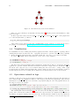
We currently provide only methods to add states and edges. Example:
>>> ts = pmlab.ts.ts_from_file(’f96q3.set.sg’)
>>> s4 = ts.add_state(’s4’)
>>> ts.add_edge(’s3’,’added’,s4)
#<Edge object with source ’2’ and target ’4’ at 0xaf2bf14>
This yields the TS in Figure 3.1. Note that we can reference vertices using the vertex descriptor or
by name.
15
16
CHAPTER 3. TRANSITION SYSTEMS
s0
L
s1
s3
L
s2
N
N
added
L
s4
Figure 3.1: TS with an added vertex and transition.
There are some technical problems with removing vertices1 , thus the preferred mechanism is to filter
states and edges.
To filter edges and vertices, use the graph tool set edge filter and set vertex filter on the graph member of the TS (with name g). That is:
ts.g.set_vertex_filter(bmap)
where bmap is a Boolean property map containing True for the vertices to be kept. Please refer to
the graph tool documentation (http://projects.skewed.de/graph-tool/doc/index.html).
3.4
Visualization
For visualization we rely on third-party libraries/applications. First of all, the graph tool package offers a
drawing function that can either use cairo or graphviz. To these two options we also added the possibility
to call the draw astg application that comes with Petrify (also expected to be in /usr/local/bin).
To draw a TS, simply call the draw function on the object. Some examples:
>>> ts.draw(’ts.png’)
>>> ts.draw(’ts_astg.ps’,’astg’)
>>> ts.draw(None, ’cairo’)
The first version writes a PNG file using graphviz (the default driver). The second uses the draw astg
application to generate a PS file. The last one is used for interactive output. However, in this last version,
the labels of the edges are lost, so it is of limited utility (also the nodes tend to overlap). Valid output
formats include PS, PDF, SVG and PNG. The output format is deduced from the filename extension.
Clearly this part needs some cleaning and modifications, but this is what we have by the moment.
3.5
Operations related to logs
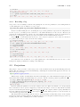
A useful operation is to incorporate frequency information to the TS states and arcs. For that purpose
there exists the map log frequencies function. The frequency information is graphically depicted in the
draw function by means of larger nodes and wider edges (when using the cairo and graphviz drivers, not
the astg). Let us see an example:
>>> log.get_uniq_cases()
defaultdict(<type ’int’>, {(’N’, ’N’): 46, (’L’,): 41,
(’L’, ’L’): 146, (’L’, ’L’, ’L’, ’L’): 64})
>>> ts.map_log_frequencies(log, state_freq=True, edge_freq=True, state_cases=True)
The resulting TS is shown in Figure 3.2. As you can see the labelling algorithm of graph tool is not
perfect, since some labels are hidden by the width of the edges, but there is a graphical representation of
the number of sequences visiting each vertex and edge. In this particular example we have also instructed
1 graph
tool reorders all vertex descriptors when one of them is removed, invalidating our dictionary that maps state
3.6. TAKING ADVANTAGE OF THE ALGORITHMS IN GRAPH TOOL
17
s0
L
N
s1
s5
L
N
s2
s6
L
s3
L
s4
Figure 3.2: TS with state and edge frequencies.
the algorithm to store the numbers of the unique sequences going through each state. The frequency can
be retrieved using the get state frequency method, while the list of unique sequences is obtained via
the get state cases method:
>>> ts.get_state_frequency(’s5’)
46
>>> ts.get_state_cases(’s5’)
array([0])
>>> log.get_uniq_cases().items()[0]
((’N’, ’N’), 46)
Some functions related to logs and TSs have been compiled into a special module:
import pmlab.log_ts
Currently there is only a single function, namely cases included in ts that returns a log containing
only the cases (and part of the cases) that fit inside the TS. Additionally, some related information is
also printed in the screen:
>>> ml = pmlab.log_ts.cases_included_in_ts(l, ts)
#Total cases in log: 7
#Excluded:
0
0.00%
#Partially Included: 1 14.29% average included length 50.00%
#Totally Included:
6 85.71%
3.6
Taking advantage of the algorithms in graph tool
The graph tool package offers a wide range of algorithms on graphs. The member g of a TS object
contains the underlying graph that can be passed as parameter to any of the graph tool algorithms.
For instance if you want to obtain the vertices of the TS ts (in this particular case this corresponds to
Figure 3.2) sorted in topological order, you can use:
>>> import graph_tool.all as gt
>>> sort = gt.topological_sort(ts.g)
>>> print sort
[5 4 3 1 6 2 0]
names to these descriptors.
18
CHAPTER 3. TRANSITION SYSTEMS
Note that these values are the internal vertex indices, so if you want to obtain the corresponding state
name, you must first obtain the vertex object, and then the name of that vertex:
>>> [ts.vp_state_name[ts.g.vertex(i)] for i in sort]
[’s4’, ’s3’, ’s2’, ’s1’, ’s6’, ’s5’, ’s0’]
Chapter 4
Petri Nets
The Petri Nets module is imported with:
import pmlab.pn
4.1
Obtaining a PN from a TS
The discovery algorithms can be accessed through the pn from ts function. The current methods are
based on the theory of regions. This function receives as parameters the discovery method to use (rbminer
or stp), the desired k-boundedness and an aggregation factor.
>>> pn = pmlab.pn.pn_from_ts(ts, k=2, agg=4)
For instance in this example the rbminer tool is used (the default one), to search for 2-bounded regions
with an aggregation factor of 4. This latter factor is ignored when using stp, which searches for ALL
minimal regions. Since no simplification is performed afterwards, it can generate more places.
4.1.1
It takes eons to finish, what can I do?
Some advices: if using rbminer, reduce the aggregation factor. Depending on the number of state of
the TS and the number of activities, smaller values might be needed to avoid a combinatorial explosion.
Values from 2 to 4 often work.
Sometimes the problem is not the aggregation factor, but the simplification step when lots of places
have been found. Rbminer includes an option to disable the simplification (currently not handled in
the python function). However it is usually better to try with other approaches, since if the simplification phase could not finish due to the large number of places, non-simplifying the net will yield an
uncomprehensible model anyway.
4.2
Loading/Saving
A PN can be saved using the save method, as usual. The target format is the SIS format.
>>> pn.save(’test.g’)
>>> pn2 = pmlab.pn.pn_from_file(’test.g’)
The function pn from file allows loading a saved PN. It infers the format from the filename extension,
unless explicitely provided. Two input formats are currently supported: SIS (.g extension) and PNML
(.pnml extension).
4.3
Visualization
Works similarly to the TS visualization. However we currently provide only support for the cairo and
draw astg drivers (simply we have not the time yet to write the code to handle the graphviz driver).
When using draw astg the valid output formats are PS, GIF and DOT.
19
20
CHAPTER 4. PETRI NETS
4.4
Simulation
The PN simulation has its own module:
import pmlab.pn.simulation
This module contains a single function, simulate, that returns a log in which all cases where obtained
by simulating the PN with the given parameters.
>>> slog = pmlab.pn.simulation.simulate(pn,method=’rnd’,num_cases=10,length=4)
>>> slog.get_cases()
[[’a’, ’b’, ’d’, ’c’],
[’a’, ’c’, ’b’, ’d’],
[’a’, ’e’, ’d’, ’f’],
[’a’, ’b’, ’d’, ’c’],
[’a’, ’c’, ’b’, ’d’],
[’a’, ’c’, ’b’, ’d’],
[’a’, ’e’, ’d’, ’f’],
[’a’, ’c’, ’b’, ’d’],
[’a’, ’c’, ’b’, ’d’],
[’a’, ’d’, ’c’, ’b’]]
Depending on the parameters, please be patient, this code has not been optimized for performance.
Chapter 5
Causal Nets
The Causal Nets module is imported with:
import pmlab.cnet
5.1
Obtaining a Cnet from a log
The easiest way to obtain a C-net that can replay the log is to use the immediately follows C-net. The
function that computes this trivial C-net is immediately follows cnet from log:
>>> cif = pmlab.cnet.immediately_follows_cnet_from_log(clog)
For more interesting C-nets we use an SMT solver, called stp. The stp solver is a little bit picky about
variable names. Moreover, logs to be used for C-net discovery have to satisfy some properties related
to the initial and final activities. Thus, this module provides a function that conditions a given log for
C-net discovery.
>>> clog = pmlab.cnet.condition_log_for_cnet(l)
Once a suitable log is available, we can use the cnet from log function. With the default parameters,
it returns a tuple whose first element is the discovered C-net, and the second one is an object containing
the binding frequencies computed. The discovered C-net has been arc minimized, and then all redundant
bindings have been removed. A skeleton (i.e., a list of activity pairs) can be provided also. The binding
frequencies can be later on used for enhancing model representation (particularly BPMN diagrams derived
from the C-net).
A nice way to obtain a reasonable skeleton is to use the heuristics of the Heuristic Miner. The function
flexible heuristic miner provides this functionality:
>>> skeleton = pmlab.cnet.flexible_heuristic_miner(clog,0.6,0.6,0.5)
>>> cn, bfreq = pmlab.cnet.cnet_from_log(clog, skeleton=skeleton)
5.2
Loading/Saving
As with other objects in the suite, the Cnet class has its own save method. The formats available are
JSON (native) or ProM (in two variants, the new and the old format). At the time of writing this
document with ProM6.1 the format is still the old one.
>>> cn.save(’test.cn’)
>>> cn.save(’test.prom.cnet’,format=’prom’)
>>> cn.save(’test.oldprom.cnet’,format=’prom_old’)
Loading is provided through the following module function:
21
22
CHAPTER 5. CAUSAL NETS
>>> cn = pmlab.cnet.cnet_from_file(’test.cn’)
5.3
Visualization
C-nets are complex to depict. We provide a prototype of interactive visualizer based on the pygame
package. Do not expect it to work correctly for large C-nets, however it will do the trick for the small
ones (this is better than nothing). Just call the draw function to start the visualizer.
>>> cn.draw()
5.4
C-net manipulation
C-nets can be merged simply by using the addition operator.
>>> cnm = cn + cif
5.5
Simulation
The simulation functions are located inside the simulation module of this sub-package:
import pmlab.cnet.simulate_cnet
fitting cases in skeleton Returns a log containing the sequences that would fit in any C-net using
the arcs in [skeleton] (regardless of the actual bindings that would be required). Useful if using a
skeleton generated using the FHM and you do not want to add elements to the skeleton to include
all the behavior of the log, but want to retain as much as the behavior of the log that can be
explained by that skeleton.
nonfitting cases in cn Returns a log with all the cases of the given log that are non-fitting in the given
C-net.
fitness Returns the fitness of the given log with respect to the C-net.
5.6
Operations related to Transition Systems
We can compute a lower bound on the ETC metric for a given TS using the etc lower bound method.
In the following example we develop a complete case from the beginning:
>>> import pmlab.log
>>> log = pmlab.log.log_from_file(’f96q3.tr’)
>>> import pmlab.cnet
>>> clog = pmlab.cnet.condition_log_for_cnet(log)
>>> ts = pmlab.ts.ts_from_log(clog, ’mset’)
>>> ts.map_log_frequencies(clog)
>>> cn, bfreq = pmlab.cnet.cnet_from_log(clog)
>>> cn.etc_lower_bound(ts)
0.902352418996893
Here we first load a log, we condition it for C-net discovery and we build a TS using the sequential
conversion (we must use this conversion to check the ETC metric) to whom we add the frequency
information. Finally, we pass this TS to the etc lower bound function that returns a lower bound on the
ETC metric. In this particular example the C-net is a very precise model, with a lower bound of 90.2%.
This value is a lower bound because the algorithm does not actually check if the escaping edges are
actually valid C-net cases (they could not, in which case the real number of escaping edges would be
inferior, thus the real ETC value would be larger).
Chapter 6
BPMN diagrams
The BPMN module is imported with:
import pmlab.bpmn
6.1
Obtaining a BPMN diagram from a Cnet
The following example show how to obtain a BPMN from a C-net derived from a log.
>>> import pmlab.cnet
>>> log = pmlab.log.Log(cases=[[’A’,’B’],[’C’,’D’]])
>>> clog = pmlab.cnet.condition_log_for_cnet(log)
>>> cn, bfreq = pmlab.cnet.cnet_from_log(clog)
>>> import pmlab.bpmn
>>> bp = pmlab.bpmn.bpmn_from_cnet(cn)
>>> bp.add_frequency_info(clog, bfreq)
Checking A
Checking C
Checking B
with E: 1 100.0% 50.0%
Checking E
Checking D
with E: 1 100.0% 50.0%
Checking S
with C: 1 50.0% 100.0%
with A: 1 50.0% 100.0%
Note that the BPMN is enhanced depicting (through the arc width in the diagram) the frequency of
each path according to the binding frequency obtained during the C-net computation, and that the log
must also be provided. The output gives tabular information: for instance, the line
Checking B
with E: 1 100.0% 50.0%
indicates that there is a single trace through the arc connecting B and E, and that this single sequence
represents the 100% of the sequences that go out from B and the 50% of the sequences that arrive to E.
The BPMN class provides also another method to enhance the output that is related to the durations
of the activities. In particular, the add activity info function takes a dictionary that maps each activity
to a dictionary containing information of the activity. If this dictionary contains the entry avg duration,
then the activities are depicted using a color scheme that represents fast activities (with respect to the
average duration of an activity) with green colors and slow activities with red colors.
To generate a DOT file containing the BPMN diagram, use the print dot function. If additional
information has been provided through some enhancement function, it will be automatically displayed.
23
24
CHAPTER 6. BPMN DIAGRAMS
6.2
Manually creating a BPMN diagram
It is perfectly possible to create a BPMN diagram from scratch or to add arcs/activities to an existing
one. Use the add element and add connection functions:
from pmlab.bpmn import BPMN, Activity, Gateway
b = BPMN()
act1 = b.add_element(Activity(’hola’))
b.add_connection(b.start_event, act1)
act2 = b.add_element(Activity(’adeu’))
b.add_connection(act2, b.end_event)
gw = b.add_element(Gateway(’exclusive’))
x1 = b.add_element(Activity(’exclusive1’))
x2 = b.add_element(Activity(’exclusive2’))
b.add_connection(act1, gw)
b.add_connection(gw, [’exclusive1’,’exclusive2’])
gw2 = b.add_element(Gateway(’exclusive’))
b.add_connection([’exclusive1’,’exclusive2’], gw2)
b.add_connection(gw2,’adeu’)
b.print_debug()
b.print_dot(’bpmn.dot’)
! dot -Tps ’bpmn.dot’ > ’bpmn.ps’
This code generates the following figure:
hola
exclusive1
exclusive2
adeu
Figure 6.1: BPMN diagram
To generate a PDF from the PS file, use the following commands:
ps2pdf bpmn.ps
pdfcrop bpmn.pdf
6.3
Loading/Saving
Currently, there are no load/save operations for this class, so you have to generate it from the C-net every
time (yes, I know, this is something we must work out at some point) or just use the Dot file generated.
Chapter 7
Module scripts
The scripts module is imported with:
import pmlab.scripts
This module contains few examples on how to use the objects and algorithms of previous modules in
order to create high-level scripts. It is a temporary module that may be removed in the future.
7.1
Obtaining a BPMN diagram from a log
The first and maybe most useful functionality provided in the module is presented below: how to discover
a BPMN diagram from a log. See the simple invocation below for an example.
>>>
>>>
>>>
>>>
import pmlab.scripts
log = pmlab.log.Log(cases=[[’A’,’B’,’F’],[’A’,’C’,’D’,’F’]])
b = pmlab.scripts.bpmn_discovery(l)
pmlab.scripts.draw_bpmn(b)
This code generates the following figure:
A
C
D
B
F
Figure 7.1: BPMN diagram
Other simple functionalities are implemented in this package (plotting charts, parallel discovery, etc.).
We advice the user to explore the file init .py.
25
26
CHAPTER 7. MODULE SCRIPTS
Chapter 8
Adding packages/modules to the
suite
To add a package foo, one should simply create a directory inside the directory where the pmlab package
is located, and inside the foo directory, create a init .py file. Then this package can be imported as
import pmlab.foo
Similarly, if one wants to create a module bar inside this package, then a bar.py file has to be create
inside the foo directory. Then the module can be imported with
import pmlab.foo.bar
However, my recomendation is that you create your scripts on your own folders, simply importing the
modules you need from the suite. These scripts can quite easily become a package or a module later on.
The idea is that if you feel your scripts add necessary/useful functionality, you can send them to us, so
that we can merge them with the “official” code. Note that the current package distribution stores the
code in terms of the objects they work on (logs, TSs, PNs, etc.). In general this is a reasonable option,
since techniques that work well for all kinds of models are, unfortunately, not very frequent.
Please try to follow as much as possible the conventions in the code:
• The function that creates an object of type X from another of type Y is usually named X from Y.
• Similarly, to retrieve X from a file (load) we usually have a function X from file.
• The function to save an object is name save.
• The function to obtain a graphical representation of an object is named draw, although we usually
keep this name if the function accepts similar parameters to the already existing draw methods.
27
28
CHAPTER 8. ADDING PACKAGES/MODULES TO THE SUITE
Bibliography
[SC10]
Marc Solé and Josep Carmona. Process mining from a basis of state regions. In Petri
Nets, volume 6128 of LNCS, pages 226–245, 2010.
[SC13]
Marc Solé and Josep Carmona. Region-based foldings in process discovery. IEEE Trans.
Knowl. Data Eng., 25(1):192–205, 2013.
[vdA11]
Wil M. P. van der Aalst. Process Mining - Discovery, Conformance and Enhancement of
Business Processes. Springer, 2011.
[vdAvDG+ 07] Wil M. P. van der Aalst, Boudewijn F. van Dongen, Christian W. Günther, R. S. Mans,
Ana Karla Alves de Medeiros, Anne Rozinat, Vladimir Rubin, Minseok Song, H. M.
W. (Eric) Verbeek, and A. J. M. M. Weijters. ProM 4.0: Comprehensive support for
real process analysis. In Int. Conf. on Applications and Theory of Petri Nets and Other
Models of Concurrency, volume 4546 of LNCS, pages 484–494, 2007.
29