Download A Poor Man`s Resistance Bridge

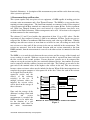
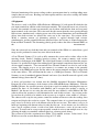
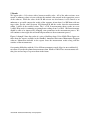
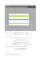
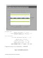
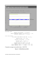
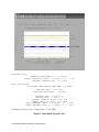
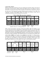
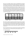
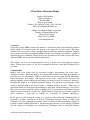
A Poor Man’s Resistance Bridge
Speaker: Gary Bennett
Fluke Corporation
PO Box 9090
Everett, WA 98206
Phone: (425) 446-6365; FAX: (425) 446-5649
Email: [email protected]
Authors: Gary Bennett Fluke Corporation
Thomas A. Marshall Data Proof
2562 Lafayette Street
Santa Clara, CA 95050
www.DataProof.com
1. Abstract
Using only a single DMM, scanner and software, a lab can have their own automated resistance
bridge capable of accuracies from sub ppm to a few ppm over its entire range. This paper
describes how we created a simple resistance bridge using off the shelf test equipment. Software
was created to take dual four-terminal DMM resistance ratio readings and control a scanner to
automate the process. Multiple forward and reverse measurements are taken to reduce the effects
of thermal EMFs and to provide statistical information.
This “bridge” can be set up to automatically scale up or down over a wide range of resistance
values. Results from various 1:1 and 10:1 measurements between 1 ohm and 10 kilohm will be
presented.
2. Introduction
Bridges have been widely used for precision resistance measurements for many years.
Automated Current Comparator Bridges are commercially available today with the capability of
providing very low uncertainties. However, their high cost prevents many smaller laboratories
from owning these new bridges. Our objective was to create a simple lower cost system for
making standard resistor comparisons for buildups of various resistor sets between 1 ohm and 1
Megohm that would fit in a smaller laboratories budget. Our parameters were that the system
would be fully automated and would require a minimum number of pieces. Each piece of
equipment should be off the shelf and multipurpose with other standard functions. Our goal for
this system was that it would be capable of making 10 to 1 measurements with about 1 part per
million or better accuracies for each step. While Current Comparators are certainly capable of
better accuracies, 1 ppm may be suitable for a majority of standards laboratories.
In this paper we will present the results of a system developed with the combined efforts of
researchers at Fluke Corporation in Everett Washington and Data Proof in Santa Clara
California. All of the equipment used in this system is available off-the-shelf and may already be
available in many standards laboratories. The measurement software was developed in California
and the testing and evaluation was performed in Washington State in the Fluke Primary
2005 NCSL International Workshop and Symposium
Standards Laboratory. A description of this measurement system and the results from our testing
of the system are presented
3. Measurement Setup and Procedure
This system requires only two pieces of test equipment, a DMM capable of making precision
resistance ratio measurements and a Low Thermal Scanner. The DMM is set up to make fourterminal resistance comparisons. The four Front terminals are connected to the A-Line output of
a Quad Scanner and the Rear terminals are connected to the scanner B-Line. In this experiment
two 320A Low Thermal Scanners were used instead of a Quad Scanner since these were
available in the Fluke Laboratory. Either arrangement can be used. All resistors to be compared
are then connected to the scanner inputs.
The software [1,2 and 3] used enables the comparison of from 1:1 up to 10:1 values. For this
experiment we first compared a known 1 Ohm to an unknown 10 Ohm. In the next run we
compared the 10 Ohm to an unknown 100 Ohm carrying each value up to 10K ohms. Whether
making a run with two resistors or more than two resistors in a run, all readings are made with
two resistors at a time until all the resistors in the run are included in the measurement. The
resistors are measured first in the forward direction with one resistor connected to the front
DMM terminals, then the measurement is reversed so the other resistor is connected to the front
terminals.
The DMM is set to read the ratio between the two resistors and the average of the forward and
reverse reading is recorded. With two resistors in the run this is repeated four times, half with
the first resistor in the second position. If more then two resistors are to be compared the
software sets up the resistors in pairs in a statistically balanced design. Any number of resistors
can be compared with this software, between two and eight. The readings are recorded as the
ppm ratio to the nominal value of the highest value resistor in the run. This was necessary
because various resistance values may be included in the run. When all the intercomparisons are
complete the program computes a least-squares-fit of the data. Values for each of the resistors
are assigned based on the leastsquares-fit results and the
value(s) of the reference
R1
Front
8508A/01
resistor(s) in the test. If
READING OHMS
multiple reference values are
Rear
included the resistor values
R2
will be based on the average of
164B
LOW
IEEE.488
these references.
THERMAL
R3
BUS
Since only the average of the
difference readings from both
forward
and
reverse
measurements is recorded, the
DMM needs to be stable only
for the duration of a pair
measurement rather than for
the
entire
measurement.
SCANNER
COMPUTER
RN
METHOD 1B: DUAL FOUR-TERMINAL CONNECTION TO DMM
2005 NCSL International Workshop and Symposium
Figure 1
Statistical monitoring of the meter readings reduces measurement time by avoiding taking more
samples than are necessary. Readings are taken rapidly until five successive readings fall within
a preset deviation.
4. Equipment
The meter we used is the Fluke 8508A Reference Multimeter [4] with option 01 which has the
rear input terminals in addition to the front input terminals. The reason this meter was selected is
because four terminal resistance measurements can be taken with both the front and rear panel
input terminals at the same time. This ratio mode has the current from the meter passing through
both resistors simultaneously, reducing errors caused by current fluctuations and environmental
effects since both resistors are affected the same way at the same time. For resistors below
20 k
a stimulus current (of alternating polarity) is applied through both resistors
simultaneously, and the potential difference measured across the resistors is scanned between the
Front and Rear Terminals. The alternating polarity greatly reduces the affect of thermal EMFs on
the
measurements.
Since the ratio mode uses both the front and rear terminals of the 8508A it is critical that a good
range zero be performed to cancel any zero offsets in the meter.
A Low Thermal Scanner [5] is used to fully automate the system and to reduce offsets in the
metering circuit. Besides switching between resistors, the scanner connects each resistor
alternately to both inputs of the DMM. The 164A Quad Scanner is ideally suited for this purpose
because it is specifically designed for making direct four-terminal comparisons between two sets
of four output connectors. Two conventional Low Thermal Scanners can also be used in this
system. The simplest way to set up two scanners is to connect one scanner to the potential
terminals of the DMM and resistor and the other to the current terminals and then set them both
to the same address. This will function the same as a 164B Quad Scanner. The Low Thermal
Scanners we used contributed minimal thermal emf errors (less than 20 nanovolts typical) with
minimal leakage (better then 1012 ohms).
A driver and procedure was written into the OhmRef Automated Resistance Maintenance
Program [6] to take advantages of the features of the 8508A/01Reference Multimeter. With the
OhmRef software, the operator can now select from several test methods including this new test
method. For those of you familiar with OhmRef you’ll recognize this method as similar to
Method 1 but because we are using the ratio mode the new method is called Method 1B. This
software allows the operator to store information for each of their resistors. Any resistor on the
list can then be selected to be include in the test run, up to eight at a time within a 1:10 ratio.
The software will set up the test pattern; control the scanner and meter to take the readings, then
compute and display the results in a report. The computed value of a resistor from the previous
run is stored so it can be used as the known value in the next test run. This makes it easy to do
build-ups beginning with known values for only the first run. A new feature was also added to
store a run or sequence of runs so with a few clicks of the mouse a series of test runs can be
repeated. Test runs can be set up to run repeatedly to make it easier to run multiple tests in a day
or during the night, to accumulate sufficient data over a shorter period of time.
The resistors used in this experiment were Fluke 742A standard resistors. Values from 1 to
10 k were used in an environment that was kept at 23°C ±0.6.
2005 NCSL International Workshop and Symposium
5. Results
We began with a 1
resistor with a known traceable value. All of the other resistors were
treated as unknown values resistors with just the nominal value entered in the appropriate screen
of the software. While the value of the 10 k resistor was also known, it was entered as an
unknown so we could compare the results of the sequence of runs from 1 to 10K ohms with our
target value. For the values between 10
through 10 k the results show the measurements
within 1 µ / of the certified values. The 1 to 10
measurement shows results just over
1 µ / . More work is continuing on getting better readings from 1 to 10 . 10 measurements
should be able to be improved by changing some parameters in the measurement process. We
will continue to investigate this and make improvements to the measurement process.
Figures 1 through 5 show the results of a series of build ups from 1 to 10 k . These figures are
taken from the reports available in the OhmRef, Automated Resistance Maintenance Program
software. Information included in the reports show the measurement results along with the
statistics of the measurements.
Overcoming difficulties with the 1 to 10 measurements caused delays in our work that did
not allow us to make the planned measurements from 10 k to 1 M . These measurements will
take place and we hope to report on them in the future.
2005 NCSL International Workshop and Symposium
UCL
MEAN
Cert. Value
LCL
dp
RESISTOR DATA:
NOMINAL RESISTANCE = 10 ohm(s)
ACTUAL CERTIFIED VALUE = 36.1 PPM (10.000361)
EXPANDED UNCERTAINTY = 1.37 PPM
DATA STATISTICS:
DEVIATION FROM NOMINAL OHM FOR: 10_ohm_U
MEAN OF DATA: 37.187 PPM
STANDARD DEVIATION: 0.195 PPM
HIGHEST VALUE IN DATA: 37.384 PPM
LOWEST VALUE IN DATA: 36.954 PPM
UPPER CONTROL LIMIT (+ 2 Sigma): 37.47 PPM
LOWER CONTROL LIMIT (- 2 Sigma): 34.73 PPM
Comparison average verses certified value: 1.087 PPM
Figure 2. 10
2005 NCSL International Workshop and Symposium
Build Up From 1
.
UCL
Cert. Value
MEAN
LCL
dp
RESISTOR DATA:
NOMINAL RESISTANCE = 100 ohm(s)
ACTUAL CERTIFIED VALUE = 3.3 PPM (100.00033)
EXPANDED UNCERTAINTY = 0.62 PPM
DATA STATISTICS:
DEVIATION FROM NOMINAL OHM FOR: 100_ohmU
MEAN OF DATA: 3.254 PPM
STANDARD DEVIATION: 0.133 PPM
HIGHEST VALUE IN DATA: 3.400 PPM
LOWEST VALUE IN DATA: 3.015 PPM
UPPER CONTROL LIMIT (+ 2 Sigma): 3.920 PPM
LOWER CONTROL LIMIT (- 2 Sigma): 2.680 PPM
Comparison average verses certified value: - 0.046 PPM
Figure 3. 100
2005 NCSL International Workshop and Symposium
Build Up From 10
.
UCL
MEAN
Cert. Value
LCL
dp
RESISTOR DATA:
NOMINAL RESISTANCE = 1 kilohm(s)
ACTUAL CERTIFIED VALUE = 4.4 PPM (1,000.0044)
EXPANDED UNCERTAINTY = 0.49 PPM
DATA STATISTICS:
DEVIATION FROM NOMINAL OHM FOR: 1k_ohm_U
MEAN OF DATA: 4.400 PPM
STANDARD DEVIATION: 0.108 PPM
STARTING DATE: 27 Apr 2005
ENDING DATE: 29 Apr 2005
HIGHEST VALUE IN DATA: 4.512 PPM
LOWEST VALUE IN DATA: 4.282 PPM
UPPER CONTROL LIMIT (+ 2 Sigma): 4.890 PPM
LOWER CONTROL LIMIT (- 2 Sigma): 3.910 PPM
Comparison average verses certified value: 0.000 PPM
Figure 4. 1 k
2005 NCSL International Workshop and Symposium
Build Up from 100
.
UCL
MEAN
Cert. Value
LCL
RESISTOR DATA:
NOMINAL RESISTANCE = 10 kilohm(s)
ACTUAL CERTIFIED VALUE = 4.2 PPM (10,000.042)
EXPANDED UNCERTAINTY = 0.50 PPM
DATA STATISTICS:
DEVIATION FROM NOMINAL OHM FOR: 10K_OHMU
MEAN OF DATA: 4.593 PPM
STANDARD DEVIATION: 0.044 PPM
STARTING DATE: 27 Apr 2005
ENDING DATE: 30 Apr 2005
HIGHEST VALUE IN DATA: 4.297 PPM
LOWEST VALUE IN DATA: 4.210 PPM
UPPER CONTROL LIMIT (+ 2 Sigma): 4.700 PPM
LOWER CONTROL LIMIT (- 2 Sigma): 3.700 PPM
Comparison average verses certified value: 0.393 PPM
Figure 5. 10 k
2005 NCSL International Workshop and Symposium
Build Up from 1 k .
6. Uncertainty Analysis
While the results show the build ups from 1 to 10 k , this uncertainty analysis will show the
uncertainties of measurements starting at 10 k and building down to 1 which gives the best
uncertainties over the greatest range. The descriptions of the uncertainty components are divided
into three parts. The components associated with the transfer uncertainty of the 8508A. The
components associated with OhmRef Method 1B. Finally, the reference resistor and the
combination of build up or build down transfers are discussed.
Table 1. Fluke 8508A uncertainty components.
8508A Transfer
Uncertainty (20min)
8508A Measurement
Uncertainty
Reference
UUT
Reference
UUT
µ /
µ /
µ /
µ /
8508A Range Nominal
Nominal Reading
Range
(URM)
(UUM)
20
10
1
0.8
0.7
2.2
14.8
200
100
10
0.2
0.15
0.5
3.2
2,000
1,000
100
0.2
0.15
0.5
3.2
20,000
10,000
1,000
0.2
0.15
0.5
3.2
Type
B
B
Distribution Normal
Normal
Confidence Limit (C.L.) or Coverage Factor (C.F.)
95%
95%
Degrees of
Freedom
200
200
200
200
Table 1 shows the uncertainty components coming from the Fluke 8508A. The 8508A is set up
to use the ratio mode for these measurements so the Transfer Uncertainty was used. The 8508A
Transfer Specification uses both µ / of reading and µ / of range specifications. These were
combined and computed separately for both the reference and UUT resistors. For example, the
10 UUT is measured using the 200 Range which has a 0.15 µ / of range specification and
0.2 µ / of reading specification. The 10 UUT will have an uncertainty of 3.2 µ / ( [0.15
µ / of 200 is 0.00003 + 0.2 µ / of 10 is 0.000002 ] / 10 * 1E+6 = 3.2). The uncertainty
contribution for the 8508A is listed under the columns labeled 8508A Measurement Uncertainty,
one column for the Reference resistance measurement and another column for the UUT
resistance measurement. The degrees of freedom for these specifications were infinite. In the
Fluke Primary Standards Lab we enter 200 for any degrees of freedom that are infinite.
Table 2. OhmRef uncertainty components.
UUT
Nominal
1
10
100
1,000
Type
Distribution
C.L. or C.F.
Effect of 1E+12
leakage
Ref
UUT
µ /
µ /
(URL)
(UUL)
0.00
0.00
0.00
0.00
0.00
0.00
0.01
0.00
B
B
Normal
Normal
95%
95%
OhmRef
Method 1B
Degrees
Type A
Degrees
of
µ /
of
Freedom
(UA)
Freedom
200
0.20
4
200
0.13
5
200
0.11
5
200
0.04
4
A
Normal
1
2005 NCSL International Workshop and Symposium
Transfer
Combined
Uncertainty
µ /
7.5
1.6
1.6
1.6
B
Normal
1
Effective
Degrees
of
Freedom
209
212
211
210
Table 2 shows the uncertainty components associated with OhmRef Method 1B. Data Proof
Scanners have a thermal EMF specification of 50nV but is typically 20nV. Because the 8508A is
in the TruOhm mode for measurements below 20 k , the 8508A reverses the current through the
resistors during the measurement process, reducing the thermal EMFs to negligible levels. The
first two columns contain the uncertainty caused by the specified leakage resistance of 1E+12 .
Again, like the 8508A section, the uncertainty for measurements of reference resistors and UUT
resistors are listed separately. The next component is the Type A component. In this case, we
have chosen to show the standard deviation of repeated measurements. For example, the 100
UUT Type A was determined by repeating the measurement six times and determining the
standard deviation of the six reported values. This shows the excellent repeatability of the entire
system. Another approach would be to use the standard deviation listed on the software report.
The column labeled Transfer Combined Uncertainty is the combination of all the components
we’ve discussed so far. Essentially, this column has the normalized, relative specification of the
resistance measurement system.
Table 3. Final combination of uncertainty components.
UUT
Value
1
10
100
1,000
Type
Distribution
C.L. or C.F.
Standard
Resistor
Uncertainty
µ /
(USTD)
0.3
0.3
0.3
0.3
B
Normal
95%
Degrees
of
Freedom
200
200
200
200
Combined
Uncertainty
µ /
(UC)
8.0
2.8
2.3
1.6
B
Normal
1
Effective
Degrees
of
Freedom
271
637
425
214
Expanded
Uncertainty
µ /
(UE)
16
5.6
4.6
3.3
B
Normal
95%
Table 3 shows the combination of the Transfer Combined Uncertainty with that of the Standard
Resistor. This brings the uncertainty from a relative relation to an absolute value. In our example
we are using the uncertainty of an ESI SR 104 10 k resistor calibrated by the Fluke Primary
Lab as our standard. This resistor is the starting point for all measurements. If measuring a 1 k
resistor, the Transfer Combined Uncertainty for the 1 k UUT is combined with the Standard
Resistor Uncertainty. However, if you are going to measure a 10
resistor then you must
combine the Transfer Combined Uncertainties of the 10 UUT, 100 UUT, 1 k UUT and the
Standard Resistor.
Below is the mathematical model for the 1 k measurement. The components listed match those
in tables 1 through 3 above. The expanded uncertainty is 2 times the combined uncertainty in this
case because the effective degrees of freedom of the combined uncertainty is so high.
UC = Combined uncertainty
Uc =
U RM
2
2
U
+ UM
2
2
U RL
+
2
2
U
+ UL
2
2005 NCSL International Workshop and Symposium
2
U STD
+
2
2
+U A
2
UE = Expanded uncertainty
K = 2
U E = k ∗U C
7. Evaluation / Conclusion
The results of these measurements were well within the 1 µ / goal for 10 through 10 k
measurements and just above 1 µ / for the 1
to 10 measurements. While the data so far is
very encouraging, we should exercise caution before drawing conclusions from such a small
number of data points.
The uncertainty of the OhmRef Method 1B is about half the uncertainty of the meter itself with
the major contributor of the uncertainty the transfer uncertainty of the Fluke 8508A. With some
work to characterize the transfer uncertainty of the 8508A in the OhmRef system the uncertainty
could be reduced to improve the overall uncertainty of the system.
While the system’ s uncertainty could never approach the uncertainty of a current comparator,
these initial measurements lead us to believe that achieving uncertainties close to 1 µ /
between 1 and 10 k are possible with a little additional work.
References
1) Kenneth L. Garcia; “AUTORES: Automated Resistance Maintenance Program”,
MSCProceedings, January 1992
2) James A. Marshall and Thomas A Marshall; ” Improving Automated Measurements for
Voltage, Resistance and Temperature”, NCX Proceedings, August 199 I
3) Thomas A. Marshall and James A Marshall, Developing Resistance Measurement Software,
MSC Proceedings, January 1993
4) Fluke 8508A Digital Reference Multimeter Users Manual, July 2002
5) Data Proof Operating Manual & Service Manual For 160B, 164B, 320B Low Thermal
Scanners, 1984-2005
6) Data Proof Automated Resistance Maintenance Program User Manual, 1994-2005
2005 NCSL International Workshop and Symposium