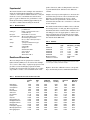
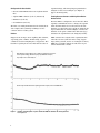
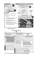
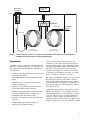
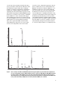
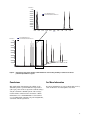
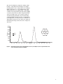
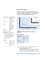
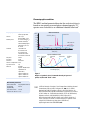
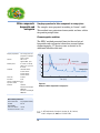
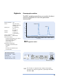
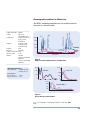
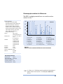
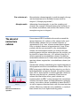
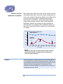
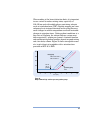
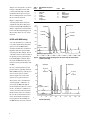
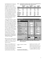
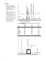
1
Solutions that meet
your demands for
food safety
testing
Excellent choices for
food applications
Productivity Tools
Applications
> Return to Table of Contents
> Search entire document
Retention Time Locking with the
MSD Productivity ChemStation
Technical Overview
Introduction
A retention time is the fundamental qualitative
measurement of chromatography. Most peak identification is performed by comparing the retention
time of the unknown peak to that of a standard. It
is much easier to identify peaks and validate methods if there is no variation in the retention time of
each analyte.
However, shifts in retention time occur frequently.
Routine maintenance procedures such as column
trimming alter retention times. In a multi-instrument laboratory running duplicate methods, the
retention times for each instrument will differ from
each other, even when run under nominally identical conditions. These differences in retention times
mean that each instrument must have a separate
calibration and integration event table, making it
time-consuming to transfer methods from one
instrument to another. Differences in retention
time also complicate comparison of data between
instruments over time.
What Is Retention Time Locking?
Retention time locking (RTL) allows a close match
of retention times on one Agilent Technologies
GC/MSD or GC system to those on another like
system with the same nominal column. By making
an adjustment to the inlet pressure, the retention
times on one system can be closely matched to
those on another system using the same nominal
column. The ability to very closely match retention
times from one system to another can greatly
reduce the time it takes to develop and transfer
methods. “RTLocked” methods can also compensate for degradations in chromatographic perfor-
mance. The ability to correct for degrading chromatographic performance, optimize lab resources,
and still provide the correct answer saves time,
money, and results in significant productivity
gains.
Using GC/MS, it is also possible to screen samples
for the presence of target compounds using a mass
spectral database of RTL spectra. The RTL mass
spectral database provides additional confirmatory information in spite of changes to the chromatographic system. One such database is the
G1672AA Pesticide RTL Library. This database
allows for quick and easy screening of pesticide
samples.
When Should I Lock My Methods?
Locking or relocking your methods should be done
whenever you make any changes to the chromatographic system or move methods from one system
to another (GC or GC/MS). To establish and maintain a locked method, RTL should be performed
whenever:
• The column is changed or trimmed
• The method is installed on a new instrument
• A detector of different outlet pressure is used
(GC vs. MS)
• System performance is validated
• Troubleshooting chromatographic problems
How Does It Work?
The process of RTL is to determine what adjustment in inlet pressure is necessary to achieve the
desired match in retention
times. To lock a given method for
the first time or for the reasons
above, you must first develop a
Retention Time vs. Pressure (RT
vs. P) calibration curve. Using an
established method, multiple
(five) injections of the standard
are used to calculate the retention times at predefined inlet
pressures. The use of an automatic sampler simplifies this
process. The RT vs. P calibration
data for each of the five injections are saved and used to correct locked methods.
chosen and then used for both
developing the locking calibration and locking all future systems. The compound, or target
peak, should be easily identifiable, symmetrical, and should
elute in the most critical part of
the chromatogram. Compounds
that are very polar or subject to
degradation should be avoided.
• Target pressure –10%
Once the target compound has
been chosen and all other chromatographic parameters of the
method have been determined,
the five calibration runs are performed. The resulting RT vs. P
calibration curve data are saved.
The software is then used to
select and integrate the peak
used for locking.
• Target pressure (nominal
method pressure)
Creating an RTL Method
The five defined pressures are:
• Target pressure –20%
• Target pressure +10%
• Target pressure +20%
Even when using columns with
the same part number (same id,
stationary phase type, phase
ratio, and same nominal length),
separate and different locking
calibration curves may be
needed. Other examples of when
separate locking calibration
curves are required include:
The following is an overview of
the actual steps taken to acquire
the RT vs. P calibration curve
data, selecting the compound/
peak to use and locking the
method.
Acquiring the RTLock Data
From Instrument Control, select
the Instrument menu and
Acquire RTLock Calibration
Data.... Agilent Technologies
GCs are the only ones supported.
See Figure 1.
If you are using an automatic
sampler, the five sample injections will be made automatically.
This example illustrates how
RTL works on a GC/MS system.
Upon completion of the fivesample analysis, Data Analysis
will begin and display the nominal MS total ion chromatogram
(TIC). If the system was configured as a stand-alone GC, all five
chromatograms will be displayed. From these displays, you
will select the compound that
will be used for RTLocking of the
method.
Selecting the RTLock Compound
Use the mouse to select the compound or peak that you would
like used for locking. For GConly mode, you must select one
peak from each of the five chromatograms for RTLocking. Once
you have made your selection,
you will be asked to allow the
software to automatically find
the remaining peaks. You may
choose to zoom the display for
better visibility. See Figure 2.
• Systems with different
column outlet pressures
(MSD/vacuum, FID/atmospheric)
• Columns differing from the
“nominal” length by more
than 15% (for example, due to
trimming)
• Systems where the predicted
locking pressure falls outside
the range of the current calibration
Selecting the Standard Compound for
RTLocking
A specific compound (usually
one found in the normal method
calibration standard) must be
2
Figure 1.
From instrument control, you select the mode of data acquisition for RTL.
Calculating the RTLock Curve and
Saving a Method
Figure 2.
Figure 3.
From this panel, the user selects the peak used for RTL. In this example the
second peak has been selected. The spectrum of the selected compound is
also displayed and is used to confirm the RTL compound.
When the RT vs. P calibration curve equation is calculated, the correlation
coefficient is determined for the RTLocked compound in each of the five
calibration samples. The resulting coefficient is displayed at each peak.
The “nominal,” or no change to pressure calibration sample, has a
correlation of 1.
Once the RTLock compound has
been selected, the new RT vs. P
curve for each compound will be
displayed. To select a new compound and calculate new RT vs.
P curves, reset the nominal
MSTIC from the RTLock menu
item. Select a new compound as
the RTL compound and from the
RTLock menu item, select Calculate New Curve from Selected
Peaks. This will generate new RT
vs. P calibration curves. The new
RT vs. P calibration curve equation will be displayed on the
screen along with the correlation
coefficient. Select Yes to either
create a new, or update an existing, RT vs. P calibration file. See
Figure 3.
Next, you can enter the name
and retention time of the
RTLock compound. See Figure 4
and Figure 5.
Figure 4.
Enter or confirm the name of
the RTLock compound.
Figure 5.
Enter or confirm the retention
time of the RTLock compound.
3
You will then be asked to confirm the RTLock pressure that
has been calculated and will be
used for that method. Select Yes
to confirm the new RTLock
pressure and save the method.
See Figure 6.
A report is also available that
provides detailed information
regarding the RTLock method.
See Figure 8. The report
includes:
• RTLock compound name
• Method name
• RTLock curve equation and
correlation coefficient data
• Calibration date
• Instrument name
• Operator name
• Status of method (on or off)
• Tabular retention time/
pressure calibration table
• Maximum deviation
• Locked retention time information (file name, acquisition
date, instrument name, and
operator name)
• Report date
Figure 6.
By selecting Yes, you RTLock
and save the method.
View Current RTLock Method Setpoints and Report
Once the system is calibrated
and locked, you can view and
confirm the RTLock setpoints by
selecting View Current Method
Setpoints. See Figure 7.
Figure 7.
Viewing the RTLock retention
times and corresponding
pressures for the RTLock
method.
Figure 8.
4
Example RTLock Report
Running an RTLock Method
Once the RTL method is created,
you can analyze and process new
samples. This requires that you
unlock and relock the methods
without editing the quantitation
calibration data. The following
example demonstrates how
retention times might change
when column maintenance is
performed or a method is moved
to a new GC/MS system. See
Figure 9. Once the method is
RTLocked, new samples are analyzed and retention times corrected. See Figure 10.
After cut
Locked
Figure 9.
Overlay of an RTLocked data file (labeled Locked) and the resulting data
file after clipping one meter off the column (labeled After Cut).
Unlocking and Relocking a Method
Once a method is locked you may
unlock or relock it using the same
or different compounds or after
additional maintenance. To
define a new compound for
RTLocking, select RTLock Setup
from the View menu in Data
Analysis. See Figure 11. The
nominal RTLock sample that represents the method you are working on will be displayed. Once
again, use the mouse to identify a
new RTLock compound.
Figure 10. Offset overlay of RTLocked data file and the RTCorrected datafile show
peaks overlapped and corrected for column maintainence.
Figure 11. To define a new compound for RTLocking, select RTLock Setup from the
View menu in data analysis.
5
www.agilent.com/chem
After selecting the compound to
RTLock, from the RTLock menu
item, select Calculate New
Curve from Selected Peaks. This
will generate a new RT vs. P calibration curve. The new RT vs. P
calibration curve equation will
be displayed on the screen along
with the correlation coefficient.
Select Yes to create a new or
update an existing RTLock calibration. See Figure 12. From the
RTLock menu you can also:
• View current setpoints
• Calculate the RT vs. P curve
• Restore the original
chromatograms
• Report the RTLock calibration
• Unlock the method
• Relock the method
Summary
RTLocking provides an easy and
flexible tool that can be used to
reduce the time and complexity
often associated with routine
chromatographic maintenance.
It allows methods to be transferred between like GC/MS systems without time-intensive
edits to the quant database and
reacquisition of standards. It
also simplifies the process for
executing routine chromatographic maintenance. RTLocking
can minimize mistakes and provide a productivity improvement
for most applications by reducing the time and setpoint
changes required to update a
method.
For More Information
For more information on our
products and services, visit our
Web site at
www.agilent.com/chem.
Figure 12. RTLock view and menu
choices.
Agilent shall not be liable for errors contained herein or
for incidental or consequential damages in connection
with the furnishing, performance, or use of this material.
Information, descriptions, and specifications in this
publication are subject to change without notice.
© Agilent Technologies, Inc. 2008
Printed in the USA
May 5, 2008
5989-8574EN
Low-Pressure Retention Time Locking
with the 7890A GC
Application
HPI
Authors
Courtney Milner and Russell Kinghorn
BST International
41 Greenaway Street
Bulleen, VIC 3105
Australia
Matthew S. Klee
Agilent Technologies, Inc.
2850 Centerville Road
Wilmington, DE 19808
USA
Abstract
Retention time locking was introduced over a decade ago
with the Agilent 6890 gas chromatograph. The next generation of GC from Agilent – the 7890A – has enhanced and
extended the functionality previously available, including
a new electronic pneumatic control system capable of
pressure control to the third decimal place. This application demonstrates the ability of the EPC system to be used
for retention time locking at low pressures, in this case
with a 320-µm column on a 5975 GC-MS.
Introduction
The introduction of retention time locking (RTL)
with the 6890 GC gave users a new way of improving productivity by eliminating the need to constantly update compound retention time data
whenever a column was trimmed or replaced. It
also allowed the same methods to be run on multiple systems with the same retention times. The
introduction of eMethods further enhanced the
portability of these methods.
Most RTL-based methods were established on
GC/MS systems, where a typical head pressure for
a 30 m × 0.25 µm id column is > 10 psi. With
setability to two decimal places, four-digit pressure
setpoints for such columns (for example, 11.54 psig)
result in excellent inter-instrument and intrainstrument RTL precision.
Amongst the many optimization tasks in GC
method development is deciding on the best
column dimension to select. This can realistically
only be determined with full knowledge of the
sample characteristics and analysis goals (that is,
components of interest, complexity, detection
limits required, and the matrix of the sample).
Larger diameter columns have the advantages of
ruggedness and sample capacity over smaller
dimension columns. The larger the diameter of the
column, the less pressure is needed to establish
optimal flows. However, for the most precise RTL,
one needs the ability to set pressure very precisely.
With two-decimal-place precision at low pressures
(for example, 1.28 psig), locking a system to a
target retention time is less precise for column
dimensions, such as 0.32-µm columns.
The 7890 GC’s fifth generation EPC provides excellent low-pressure control, and with third-decimalplace control of the pressure, providing the
precision demanded for RTL at low pressures. This
application explores the suitability of the 7890 for
RTL at low pressures with a 320-µm column and
uses a translation of the method described in Agilent Technologies publication 5989-6569EN, “Reliable transfer of existing Agilent 6890/5973GC/MSD
methods to the new 7890/5975 GC/MSD.”
Experimental
The method used for this example was translated
using the Agilent Method Translator software to
convert to a 250-µm id column method to a 320-µm
method. A series of standards was run from 10
ppb to 5 ppm to illustrate the performance of the
method, followed by trimming approximately 45
cm off the column and relocking the method.
Table 1.
Carrier gas
RTL peak
Split/splitless inlet
Oven
Sample
MSD
HP-5 25 m × 0.32 µm × 0.52 µm
p/n 19091J-112
Helium, constant pressure mode –
nominal 3.761 psi
Fluoranthene at 11.112 min
300 °C, pulsed splitless 7 psi for 0.3 in,
50 mL/min purge at 0.75 min
55 °C (1.1 min) to 320 °C (6.5 min) at
22.88 °C/min
1-µL injection, PAH 0.01 to 5 ppm
concentration range
Scan 45–400 u
Samples = 22
Autotune EM + 200V
Source = 230 °C
Quad = 150 °C
Transfer line = 280 °C
Results and Discussion
The test sample with 16 polynuclear aromatic
hydrocarbons (PAHs) was chosen for this example
as it covers a wide range of physical properties and
provides several challenging separations. This
requires the retention time precision to be as tight
as possible to ensure correct identification of the
The initial retention times in Table 2 were achieved
at a head pressure of 3.761 psig. This setpoint was
determined from the retention time calibration and
relocking process to be appropriate to achieve the
target retention time of 11.112 min for the locking
compound fluoranthene. Table 3 shows the calibration data from the RTL runs.
Table 3.
RTL Data
Run
RTLOCK1.D
RTLOCK2.D
RTLOCK3.D
RTLOCK4.D
RTLOCK5.D
Maximum deviation
Correlation co-efficient
Pressure
(psi)*
Retention
Deviation
time (mins) (seconds)
3.01
3.38
3.76
4.14
4.51
11.212
6.018
11.166
3.264
11.112
0.000
11.070
–2.508
11.020
–5.508
6.018 seconds
0.999
* Even though pressure setpoints used for RTL calibration need only be to be to two
decimal places, the ability to precisely set locking pressures based on the calibration curve requires setability to the third decimal place.
Figure 1 shows the calibration curves corresponding to the linearity metrics summarized in Table 2.
Retention Time Precision of Low-Pressure RTL
Naphthalene
Acenapthylene
Acenaphthene
Fluorene
Phenanthrene
Anthracene
Fluoranthene
Pyrene
Chrysene
Benz[a]anthracene
Benz[b]fluoranthene
Benz[k]fluoranthene
Benz[a]pyrene
Indeno[1,2,3-cd]pyrene
Dibenz[a,h]anthracene
Benzo[ghi]perylene
2
Samples were injected in triplicate to measure the
retention time precision of the locked method at
different concentrations from 0.01 to 5 ppm.
Table 2 shows the performance metrics for the
retention time and also the correlation co-efficient
for the analysis.
Method Conditions
Column
Table 2.
peaks of interest, and relocking must be effective
or peak identification will fail on the different
column.
Average
retention
time
RSD
(%)
Calibration
linearity (r2)
5.884
7.753
7.968
8.562
9.702
9.752
11.119
11.388
12.808
12.855
14.285
14.314
14.815
17.088
17.098
17.725
0.055
0.045
0.044
0.048
0.089
0.044
0.031
0.090
0.094
0.046
0.045
0.069
0.035
0.051
0.066
0.089
0.997
0.997
0.997
0.997
0.997
0.996
0.996
0.996
0.996
0.997
0.995
0.995
0.996
0.996
0.995
0.997
RT before
relocking
Relocked
RT
5.809
7.676
7.893
8.486
9.621
9.671
11.041
11.308
12.719
12.774
14.168
14.201
14.686
16.890
16.903
17.508
5.876
7.746
7.959
8.556
9.692
9.746
11.116
11.383
12.799
12.849
14.277
14.306
14.807
17.074
17.082
17.709
ΔRT when
relocked
0.008
0.007
0.009
0.006
0.010
0.006
0.003
0.005
0.009
0.006
0.008
0.008
0.008
0.014
0.016
0.016
4500000
4000000
Naphthalene
Acenapthylene
Acenaphthene
Fluorene
Phenanthrene
Anthracene
Fluoranthene
Pyrene
Chrysene
Benz[a]anthracene
Benz[b]fluoranthene
Benz[k]fluoranthene
Benz[a]pyrene
Indeno[1,2,3-cd]pyrene
Dibenz[a,h]anthracene
Benzo[ghi]perylene
3500000
Response
3000000
2500000
2000000
1500000
1000000
500000
0
0
1000
2000
3000
Concentration ppb
4000
5000
6000
Figure 1. GCMS calibration curves for 16 PAHs using 320-µm id column with low-head pressure.
Figure 2 presents overlayed chromatograms for the
replicate sample injections, showing the excellent
precision of the replicate injections summarized in
Table 2.
Abundance
3000000
TIC: 1802024.D\data.ms
TIC: 1801023.D\data.ms
TIC: 1803025.D\data.ms
2600000
2200000
1800000
1400000
1000000
600000
200000
9.60
9.80
10.00
10.20
10.40 10.60
Time
10.80
11.00
11.20
11.40
Abundance
3800000
3400000
3000000
2600000
2200000
1800000
1400000
TIC: 1802024.D\data.ms
TIC: 1801023.D\data.ms
TIC: 1803025.D\data.ms
1000000
600000
200000
4.00
6.00
8.00
12.00
10.00
14.00
16.00
18.00
Time
Figure 2.
Overlay of three replicate injections of 2 ppm standard prior to column maintenance and relocking,
including a zoomed area of the four peaks from phenanthrene to pyrene.
3
A 45-cm length of column was removed from the
column to simulate typical maintenance that may
be performed on a column during routine use. The
method was then relocked and the sample re-run
to check the efficacy of relocking at low pressure.
The relocked method had a resulting pressure of
3.168 psig. The change in locking pressure can,
over time, provide guidance as to the extent at
which column trimming can be undertaken without the need for full re-locking of the method.
Figure 3 shows an overlay of the before and after
column trimming and the extent of the retention
time change. Figure 4 presents an overlay of chromatograms, one of the originals and one after
column trimming and relocking. The last two
columns of Table 2 compare the relocked retention
times of target compounds to the originals.
Abundance
1e+07
9000000
8000000
7000000
6000000
5000000
4000000
3000000
2000000
1000000
0
TIC: RELOCK1.D\data.ms
TIC: 1902027.D\data.ms
9.40 9.60 9.80 10.00 10.20 10.40 10.60 10.80 11.00 11.20 11.40
Time
TIC: RELOCK1.D\data.ms
Abundance
TIC: 1902027.D\data.ms
1e+07
9000000
8000000
7000000
6000000
5000000
4000000
3000000
2000000
1000000
0
4.00
6.00
8.00
10.00
12.00
14.00
16.00
18.00
Time
Figure 3.
4
Overlay of injection before and after column maintenance showing the extent of retention time variation,
including a zoomed area of the four peaks from phenanthrene to pyrene
Abundance
1e+07
9000000
TIC: 1901026.D\data.ms
TIC: RELOCKCHECKA.D\data.ms
8000000
7000000
6000000
5000000
4000000
3000000
2000000
1000000
0
9.60
9.80
10.00
10.20
10.40
10.60
Time
10.80
11.00
11.20
11.40
TIC: 1901026.D\data.ms
TIC: RELOCKCHECKA.D\data.ms
Abundance
1e+07
9000000
8000000
7000000
6000000
5000000
4000000
3000000
2000000
1000000
0
4.00
6.00
8.00
10.00
12.00
14.00
16.00
18.00
Time
Figure 4.
Overlay of injections before and after column maintenance and relocking, including a zoomed area of the four
peaks from phenanthrene to pyrene.
Conclusions
For More Information
This application demonstrates the ability of the
7890 GC system to perform RTL at low pressures
(sub 5 psi), such as those experienced when using a
320-µm column in a GC-MS system. The average
retention time variation before and after column
maintenance for a 16-PAH mixture is less than 0.5
sec, providing high confidence in peak assignments,
even with critical separations.
For more information on our products and services,
visit our Web site at www.agilent.com/chem.
5
www.agilent.com/chem
Agilent shall not be liable for errors contained herein or for incidental or consequential
damages in connection with the furnishing, performance, or use of this material.
Information, descriptions, and specifications in this publication are subject to change
without notice.
© Agilent Technologies, Inc. 2008
Printed in the USA
July 11, 2008
5989-8366EN
Case Study for Agilent Lab Monitor and
Diagnostic Software
Application
HPI, Environmental, Food Safety
Author
Chunxiao Wang
Agilent Technologies (Shanghai) Co. Ltd.
412 Ying Lun Road
Waigaoqiao Free Trade Zone
Shanghai 200131
China
Abstract
Agilent Lab Monitor & Diagnostic (LMD) software can
monitor in real time all the Agilent GCs and LCs in your
lab. It automatically tracks supply usage, monitors chromatographic quality, and notifies you of maintenance
needs before a problem occurs by keeping track of injections, hours of operation, and other parameters that you
specify. Two case studies are given demonstrating some
of the features and benefits of this software.
Introduction
Agilent Lab Monitor & Diagnostic (LMD) software
is an innovative tool to help you manage your lab
to ensure performance, productivity, and reliability. LMD software can monitor in real time a single
Agilent GC or LC or all the Agilent GCs and LCs in
your lab. It automatically tracks supply usage,
monitors chromatographic quality, and notifies you
of maintenance needs before a problem occurs by
keeping track of injections, hours of operation, and
other parameters that you specify. LMD software
“knows” when it's time to replace consumables or
perform basic upkeep. It provides full diagnostic
capabilities with an extended list of tests and calibration procedures and automates basic diagnostic
routines that help verify proper instrument performance. The software is coupled with an extensive
suite of user information Help functions that provide quick, easy access to maintenance information, such as manuals and videos, so that you can
get the information you need right when you need
it.
LMD provides the following features and benefits:
• Increases your lab’s uptime by alerting you to
problems before they happen
• Provides intuitive help with diagnostic capabilities and easy-to-follow repair procedures in
case of a problem
• Enhances diagnostics and troubleshooting functionality with searchable, complete user information capability
• Keeps your systems in top condition and helps
with routine troubleshooting
• Maximizes column and consumables utilization
by optimizing replacement schedules
• Helps you meet regulatory requirements by
keeping all maintenance, event, and run logs in
a single, easily accessible location
• Provides a link to the optional, Web-enabled
Remote Advisor to back up your internal service and support resources
The following two case studies demonstrate some
of the features and benefits of the Agilent LMD
software.
Configuration for Case Studies
• One PC with LMD monitors two Agilent 7890A
GCs
• Agilent LMD software (A.01.03, Advanced)
• Firmware (A.01.06)
• ChemStation (B.03.02)
The first case study demonstrates the feature/benefit of right advice/alarm by tracking resource
counters before results go bad.
Problem
Oxygen is an enemy to most capillary GC columns,
especially polar columns. In this study, a polar
column is used for analyzing trace oxygenates. The
baseline is getting worse after 400 runs because of
septum leakage, which may impact quantitative
analysis for trace-level analysis (see Figure 1,
upper chromatogram).
Tracking Resource Counters and Giving Alarm Before
Results Go Bad
Because LMD is configured to track the GC’s inlet
septum, it reminds the user to change the septum
when the limit has been reached, before the GC
baseline goes bad. After the septum is changed, the
expected baseline is obtained. Figure 1 shows the
baseline of the polar column after 400 runs (top)
and after the septum has been changed (bottom).
LMD can track not only the inlet septum, but also
other GC resources, like the inlet o-ring, oxygen
traps, inlet gold seal, and so on. As Figure 2 shows,
LMD gives real-time indicators and alerts of preventive maintenance needs.
After 400 runs, the baseline (polar column) is getting worse because
of the septum leakage, which may impact quantitative analysis,
especially for trace level analysis.
Get the expected baseline after replacing the inlet septum, based on LMD advice.
Figure 1.
2
Baseline chromatograms on polar column after 400 runs and after the inlet septum has
been replaced.
Real-time indicators
and alerts of preventive
maintenance needs
Four Alert Actions:
Set Not Ready
Set Service Due
Email
Text Message
Setup value of
Warning, Limit
Figure 2.
LMD real-time indicators and alerts of preventive maintenance needs.
Figure 3.
Alert email for when the front inlet septum limit has been reached.
Four alert actions are available: Set Not Ready, Set
Service Due, Email, and Text Message. For example, when the email alert action is selected, LMD
will send an alert email to the users you specify.
Figure 3 shows an example email alert informing a
user that the front inlet septum’s limit has been
reached.
An email alert is configured in only three steps:
1. Manage the users (see Figure 4)
2. Manage the alerts (see Figure 5)
3. Configure the maintenance indicators
3
Procedure
1. Select Lab Monitor Management > Users
2. Add a graphic for the user if you like
3. Select “Email” from the Method pull-down menu.
4. Enter the first email address for your distribution list in the Parameter field. Select
“Add.” Add as many email addresses to your distribution list as you like.
5. Select “Apply Changes” when you have added all the email addresses.
1
2
3
4
5
Figure 4.
Procedure for managing users.
2
3
1
4
Procedure
1. Select Lab Monitor Management, Manage > Alerts.
2. Enter the address for the email server of the LMD PC network; this needs to be
provided by the customer IT department.
3. Use the default Port 25 unless the IT department instructs you otherwise.
4. Select the email recipients from the distribution list that was created in the
Users menu.
5. Select “Apply” to save these entries.
5
Figure 5.
4
Procedure for managing alerts.
1
2
Procedure
1. Edit parameters and click the icon that allows for selection of diagnostic counters.
2. Select the counters that you want to use within LMD.
Figure 6A. Procedure for configuring maintenance indicators. Set up the resource counter within ChemStation/Workstation.
Procedure
3. Select “Maintenance Indicators”
4. Select counters that you want to use within LMD
5. Setup the same counters within LMD “Maintenance Indicators
6. “Reset Value” sets the count back to 0
7. “Save changes” accepts your selections for Warning and Limit values
Figure 6B. Procedure for configuring maintenance indicators. Set up the same counter within LMD.
In this example, a warning email will be sent at 350 injections on the front inlet liner. At 400 injections the GC will be set to
“Not Ready,“ thus stopping the sequence, and an email will be sent to the distribution list that was set up in the previous
procedure (see Figure 4).
5
For the 7890A GC, the resource counters must first
be enabled from ChemStation before they will
count within LMD (see Figure 6A). Next, the same
counters are set up within LMD maintenance indicators (see Figure 6B).
2. Run SS inlet 7890A pressure decay test to confirm a leakage. Result: Failed. The above tests
indicate that there is leakage in the inlet
system. The procedures and result are shown in
Figure 9.
The next case study demonstrates how LMD can
provide intuitive help and easy-to-follow procedures in case there is a problem with diagnostic
capabilities. It also illustrates how the complete,
searchable user information enhances the diagnostic and troubleshooting functionality of LMD.
3. Solve the inlet leak problem by tightening the
column fittings, base gold seal fitting, split vent
trap housing, septum nut, and the latch to the
SSL inlet. Result: These actions don't work.
Problem
The trace level peak was lost or its response
reduced on the 7890A GC with FID and capillary
column. In this scenario, the response of ethylbenzene is reduced and m-oxylene is lost, as shown in
Figure 8.
Designing Diagnostics and Tests to Solve Specific
Problems
This problem may be caused by inlet leakage. The
diagnostic tests of the LMD software simplify complex troubleshooting tests for the user by automatically performing specific troubleshooting-related
tasks. For example, the inlet leak and inlet decay
tests helps the user with quick diagnostics, and the
FID checkout test helps verify proper performance
with convenient guidance. The problem can be
fixed efficiently with the intuitive help of LMD.
When an LMD test is running the GC Remote light
comes on, indicating control of the GC. At this
time, the ChemStation must be closed to run the
LMD tests.
1. Run SS inlet 7890A leak check. Result: Failed.
The procedures and result are shown in
Figure 8.
4. Replace the inlet septum and the liner O-ring.
User document search capability makes it easy
to find instructions on how to change the consumables, including the inlet septum and liner
O-ring. Also, detailed consumable information,
including part number, helps you select the
right part (see Figure 10).
5. Run the SS inlet pressure decay and leak check
tests. Result: Passed. See Figure 11.
6. Run the FID checkout test to confirm that the
GC system is operating properly. Before the
detector checkout test can run, you have to
install the appropriate consumable parts; that
is, an evaluation column, HP-5 30 m x
0.32 mm x 0.25 µm (p/n 19091J-413); an FID
performance evaluation (checkout) sample
(p/n 5188-5372) is also needed. The software
will prompt you when you are required to perform a task or answer a question. When the FID
detector checkout test is finished, restore the
instrument to normal operating conditions.
Result: Passed. See Figure 12.
7. Run trace-level aromatic sample. The expected
result is obtained as shown in Figure 13 after
diagnostics and troubleshooting.
8. The GC system is fixed.
• The response of ethylbenzene is reduced and m-oxylene is lost.
• Inlet leakage may be the reason. Intuitive help for diagnostics
is available from LMD.
Figure 7.
6
Trace level peak lost or response reduced on 7890GC with FID and capillary column.
Test procedure
Test result shows there is
leakage in inlet system
Figure 8.
Procedure and result for SS inlet leak check test.
Figure 9.
Procedure and result for SS inlet pressure decay test.
7
Procedure
User document search capability gives the
instructions:
1. Type “inlet liner,” then click Go for
searching.
2. Select Maintaining your GC>100......, then
you can get the instructioins.
3. Instructions on how to change the inlet
septum and liner O-ring
4. Click Replacement O-ring for detailed
information on consumables and parts for
SS inlet, including part number.
Figure 10. Searchable, complete user information capability allows for enhanced diagnostics and
troubleshooting functionality.
Figure 11. The result passed both inlet leak check and pressure decay test after troubleshooting.
8
Figure 12. The result has passed FID checkout test.
Figure 13. Expected result for trace-level aromatic sample is obtained after troubleshooting with intuitive help
from LMD.
9
www.agilent.com/chem
Conclusions
Agilent Lab Monitor & Diagnostic (LMD) software
is a new tool to help ensure the productivity, performance, and reliability of instruments in the lab.
LMD monitors multiple instruments in the lab continuously in real time and detects maintenance
needs and instrument problems before a problem
occurs. These case studies demonstrated the benefits of Agilent LMD software for customers.
• Right advice before results go bad
Real-time instrument monitoring tracks the
number of runs or the life of GC resources, such
as inlet septa, liners, and o-rings. Then, when
the user-specified limit has been reached, LMD
generates an Alert Action, for example, it sends
an alert email to specified user(s).
• Intuitive help in case of a problem
•
•
Easy-to-use system tests, including an inlet
leak test and inlet decay test, will help you
do quick diagnostics.
•
A detector checkout test will provide con
venient guidance to help you verify proper
performance.
• Extensive user document search capability
LMD offers easy-to-find and easy-to-use instructions on how to change the consumables,
including the inlet septum and liner O-ring, and
detailed consumable information, including
part numbers, to help you select the right parts.
For More Information
For more information on our products and services,
visit our Web site at www.agilent.com/chem.
Diagnostics and tests will help you solve
problems and verify proper performance.
Agilent shall not be liable for errors contained herein or for incidental or consequential
damages in connection with the furnishing, performance, or use of this material.
Information, descriptions, and specifications in this publication are subject to change
without notice.
© Agilent Technologies, Inc. 2008
Printed in the USA
May 15, 2008
5989-8613EN
Capillary Flow Technology for GC/MS:
A Simple Tee Configuration for Analysis
at Trace Concentrations with Rapid
Backflushing for Matrix Elimination
Application
Environmental, Drug Testing, and Forensics
Author
Harry Prest
Agilent Technologies Inc.
5301 Stevens Creek Blvd.
Santa Clara, CA 95051
USA
Abstract
Capillary Flow Technology devices offer the potential to
enhance GC/MSD operation and robustness. In operation,
they can allow rapid service of the GC column and inlet,
including liner and septum, without venting or subjecting
the MSD to air. In terms of robustness, late eluting compoundscan be removed from the column by "backflushing," which forces components to retreat through the
column into the injection port before they damage the
MSD source or compromise the next analysis. This leads
to higher analytical integrity as both the column phase
and the MSD can be protected. This application describes
a simple arrangement for Capillary Flow Technology
devices that provides ventless maintenance features with
highly accelerated backflushing and minimal losses in the
MSD signal. This solution supports GC analysis in constant flow mode with pressure pulsed injections and is
recommended for all MSD users (in both electron impact
or chemical ionization modes), including those with diffusion pump systems.
Introduction
The introduction of Electronic Pressure Control
(EPC) was a major advance for GC and especially
GC/MS analysis. EPC allowed development of the
constant flow mode of analysis, which generates
chromatographic peaks of consistent width (time)
and allows optimization of MS cycle times to meet
either qualitative or quantitative requirements.
Also, splitless injections gained pressure pulsing
or ramped flow modes, which lowered the analytes’ residence time in the hot injection port and
confined the expansion of the injection solvent
(avoiding overfilling of the liner). The power of this
approach lead to continued evolution of EPC technology with the present state of the art represented
in the new 7890A GC.
The recent addition of Capillary Flow Technology
(CFT) devices has reinvigorated and recast Deans
switching and other pressure control approaches
to GC analysis. One such CFT device, the QuickSwap [1–3], provides two important capabilities to
GC/MS:
1) The ability to service and/or replace the entire
analytical column or the injection port liner
and septum without venting the MSD (yet still
retaining high vacuum integrity)
2) The ability to remove from the column late-eluting, highly retained components that elute after
the target compounds of analytical interest by
reversing the carrier flow direction through the
column in what is called “backflushing.” With
the oven temperature elevated and the flow
reversed, these very high boiling interferences
can be pushed off the column into the split vent
and thereby prevent degradation of the column
phase or the detector.
A schematic representation of the arrangement
that makes this possible is shown in Figure 1.
1 to 4 psi
Aux
Aux EPC
EPC
During
GC
run
0.8 to 2.5 mL/min
Split Vent
Σ
Z mL/min
S/SL Inlet
30 m
17.1 cm
Quickswap
MSD
MSD Optimum
< 1.5mL/min
10 to 75 psi
After
GC
run
10 to 25 mL/min
S/SL Inlet
2 psi
Figure 1.
Aux EPC
Split Vent
30 m
MSD
Quickswap
Schematic of QuickSwap arrangement.
Every new approach has a downside and for
QuickSwap it is the additional makeup flow
required to purge the QuickSwap device during
analysis which dilutes the signal in the GC/MSD.
This is not an issue for many users since the sensitivity of the MSD is usually more than adequate.
However, analysis at trace concentrations has
more stringent requirements and maintaining a
signal closely comparable to that of a single continuous column is essential.
Another CFT configuration for GC/MSD applications designed specifically for trace GC/MS analysis where customers do not wish to surrender
signal is possible using the QuickSwap or any of
several other CFT devices. In this alternate configuration, the CFT device is located in the middle of
the analytical column, essentially splitting the
column in half. For example, a 15-m column preceeds and follows a CFT tee. Schematically this
arrangement is illustrated in Figure 2. The auxiliary EPC device adds just enough pressure (flow)
to match the flow (pressure) from the first column,
so there is little flow addition and therefore less
“dilution” and loss in the GC/MSD signal. Backflushing is similarly simple; the pressure or flow is
dropped in the first column section while the
second section column flow is increased.
2
17.1 cm
Advantages of this pressure controlled tee (PCT)
approach are similar to those of QuickSwap, such
as:
• Service of injection port liner and septum without venting the MSD
• Column cutback or replacement of the “front”
or first column without venting the MSD
But additional advantages of the PCT arrangement
over QuickSwap are:
• Minimal or no signal loss (in EI- or CI-MS) is
obtained because of the very small additional
“makeup” gas flow.
• Constant flow mode and pressure pulsed
injections are straightforward.
• This configuration is suitable for diffusion
pumped systems and allows backflushing in
diffusion pumped systems.
• Backflushing is more rapid and can be initiated
earlier.
This application details some configurations and
provides an example of backflushing.
Pressure/flow
controller
Split/splitless
injection port
Vent
7890A GC
Z mL/min
CFT Device
Z mL/min
5975C MSD
EI mode
Z mL/min
15-m HP-5 ms
(0.25 mm id × 0.25 µm)
Figure 2.
15-m HP-5 ms
(0.25 mm id × 0.25 µm)
Schematic of pressure controlled tee arrangement for the GC-MSD: solid lines indicate the forward flow during
GC/MSD analysis and the dashed lines indicate backflushing flows.
Experimental
A number of devices can be used in this approach
and those arrangements will be cited later, but for
these experiments the instrument configuration
was as follows:
• 7890A GC with split/splitless ports in front and
back and a 7683B ALS
• 5975C MSD with performance turbomolecular
pump
• 2 HP-5ms 15 m × 0.25 mm id × 0.25 µm film
columns (19091S-431)
• CFT device: 2-way unpurged splitter (G318160500) with SilTite ferrules and nuts
• CFT GC mounting hardware: dual-wide mounting bracket (G2855-00140) or single-wide
mounting bracket kit (G2855-00120)
• Deactivated 0.25 mm id column approximately
1 m long
As an overview of the configuration, the 1-m
column was connected to the back injection port
and to the first position on the CFT splitter using
the appropriate SilTite fittings. (This CFT device
has three connection points and is really best
thought of as a simple tee reminiscent of glass Yor T-connectors and will be referred to as a “CFT
device” or “CFT tee” from here forward).
One of the 15-m HP-5ms columns was connected at
the uppermost position on the CFT tee and the
other end through the transfer line into the MSD
as usual. The other 15-m HP-5ms column was connected to the midpoint of the CFT device and the
front injection port.
In detail, the arrangements were as follows. The
CFT tee was attached to the forward position on
the mounting hardware on the right side in the GC
oven. The 1-m long section of guard column was
wound on a spare column cage and hung on the
column hanger in the back of the oven. (This could
simply be added to one of the 15-m HP-5ms column
• 2 CFT blanking plugs (G2855-60570 or as
G2855-20550 with G2855-20593)
3
cages to avoid the extra cage.) Using a Vespel/
graphite ferrule, one end was connected to the
back injection port and the other end to the lowest
connection of the CFT device with a SilTite ferrule
and nut. The other two CFT tee connections were
sealed with CFT blanking plugs and the back injection port was pressure tested as described in the
7890A Advanced User Guide (part number G343090015).
One of the 15-m columns was then hung on the
cage carrying the 1-m column and installed with
one end through the MSD transfer line. Since this
column (column #2) can be expected to have a
rather long life as it will be protected by the
upstream column, a SilTite ferrule is recommended for the transfer-line seal. These ferrules do
not develop leaks as the transfer-line temperature
is cycled; however, the Vespel/graphite ferrules can
shrink and develop leaks. (Note that if the surface
of the transfer line is very worn it may fail to seal
well, in which case the Restek Agilent interface
cleaner [P/N 113450] can be used to resurface the
sealing surface if very carefully employed). The
other end of this GC column was connected to the
uppermost connection on the CFT tee with the
SilTite ferrule.
The “upstream” 15-m GC column (column #1) was
hung on the other 15-m column cage and installed
in the front split/splitless injection port with a
Vespel/graphite ferrule, liner, and BTO septum, as
usual. The other end was connected to the CFT tee
middle post and, after temporarily removing the
other connected columns, blanked off and pressure
tested as above.
All connections were then re-established to the
CFT tee with the 1-m column in the lower position;
the front, first column (#1) connected in the
middle position; and the rear, second or MSD
column (#2) in the uppermost connection. Helium
was supplied to both the front and back ports, and
a helium leak detector was used to check for any
leaks.
A picture of the arrangement is shown in Figure 3.
To MSD –
second
column
From front
inlet – first
column
From back
inlet – flow
control
Figure 3.
4
Picture of the installed pressure controlled tee arrangement for the GC/MSD.
GC Configuration
Operating with Pressure Pulsed-Splitless Injection
The GC can be configured in several ways. However, for instructional purposes and those of these
experiments, the GC was configured as follows:
Figures 4A and 4B show screen captures of the
7890A GC configuration for a standard pressurepulsed splitless injection with constant flow mode
operation; they show the front and back injection
port parameters. Remember, the arrangement is
set up such that the front port, into which the
sample will be injected, is configured as if a 30-m
column were installed into the MSD. Typical pressure-pulse conditions are set for these parameters:
a 25 psi pulse for 0.5 minutes; split flow on at
0.75 minutes at 50-mL/min; with gas saver on at
2 minutes at 15-mL/min. The general rules apply
for pressure-pulsed splitless injections: given a
particular liner, inlet temperature, injection
volume, and solvent, the expansion of the solvent
is confined to a fraction of the interior volume
(< 0.75) of the liner by the pressure applied.
Column #1:
Inlet:
Outlet:
Mode:
Column #2:
Inlet:
Outlet:
Mode:
30 m × 0.25 mm id × 0.25 µm column
Front injection port: pulsed
splitless mode, split flow
15 mL/min
MSD (vacuum)
Constant flow
15 m × 0.25 mm id × 0.25 µm column
Back injection port: split mode,
split flow 15-mL/min
MSD (vacuum)
Constant flow
The flows were set to 1.2-mL/min, all zones were
left cold, and the MSD power was turned on. With
the MSD and GC zones still “cold,” the MSD background was checked to be sure m/z 28 was
decreasing, indicating that the system was tight.
Only after there was confidence that there was no
leak were other zones brought up to temperature.
Figure 4A (upper panel).
Figure 4B shows that the back injection port is
in split mode, at 120 °C (to remove water background), with split flow and gas saver set at
15-mL/min flow.
Typical pressure-pulsed splitless injection parameters for constant flow:
front injection port.
5
Figure 4B (lower panel).
Typical pressure-pulsed splitless injection parameters for constant flow:
back injection port (not used for injection but for column control).
Figures 5A and 5B show the constant flow mode
settings for the two columns. The front column
flow is the typical 1.20 mL/min, but the back
Figure 5A (upper panel).
6
column flow is slightly higher at 1.25 mL/min to
prevent any backflow. Essentially the additional
flow is equivalent to an extra meter of column
length.
Typical pressure-pulsed splitless injection parameters for constant flow: First
column section (configured as a 30-m column).
Figure 5B (lower panel).
Typical pressure-pulsed splitless injection parameters for constant flow: Second
column section (configured as a 15-m column).
Results and Discussion
column configuration. Both peak height and area
remain the same, indicating that there is no loss in
Figure 6 shows the results for pressure-pulsed
signal. This is as expected since no signal dilution
splitless injections of octafluoronaphthalene (OFN) is taking place. There is a slight degradation in S/N
at 1-pg/µL acquired in selected ion monitoring
for the CFT tee results as the background noise is
(SIM) with the two 15-m column and CFT tee conraised by about 35% due to the additional flow configuration and the standard 30-m continuous
troller. The important point is that the signal is
preserved at trace levels.
CFT tee
Abundance
Standard 30-m column
5.00
5.05
5.10
5.15
5.20
5.25
5.30
5.35
5.40
5.45
5.50
5.55
5.60
5.65
5.70
5.75
5.80
5.85
Time
Figure 6.
Reconstructed total ion chromatogram (RTIC) of three replicate SIM acquisitions of octafluoronaphthalene using pulsed splitless injection with CFT tee (left profiles) and with a standard 30-m continuous
column configuration (right profiles).
7
PCT relative to the linear velocity suggests a
relatively rapid transit through the device.
Chromatographic Character
Another common chromatographic test used in
organochlorine pesticide analysis (as in USEPA
method 8081) examines degradation of 4,4'-DDT
and Endrin. This degradation test was developed
to indicate the degree of activity of the injection
port by examining the amounts of DDD and DDE
products of DDT and the ketone and aldehyde
products of Endrin. The situation is complicated
here as the degradation products can be generated
in both the injection port and the CFT tee. How-
Abundance
Beyond preserving signal, the CFT device should
exhibit reasonable chromatographic performance.
One indication of chromatographic integrity is the
peak shape profiles of the fatty acid methyl esters
(FAMEs). The result for GC/MS analysis of a
FAMEs standard acquired using a metabolomics
method is shown in Figure 7 and suggests very
little degradation of chromatography using this
PCT. This can be expected as the path is deactivated and the path length in the channels in the
6.00
8.00
10.00
12.00
14.00
16.00
18.00
20.00
22.00
24.00
Time
18.50
18.70
18.90
Abundance
18.30
6.00
8.00
10.00
12.00
14.00
16.00
18.00
20.00
22.00
24.00
Time
Figure 7.
8
Reconstructed total ion chromatogram (RTIC) of a multicomponent FAMEs standard using pulsed splitless
injection with CFT tee (upper) and the reconstructed extracted ion chromatogram (REIC) for m/z 74. The
enlarged panel is for octadecanoic methyl ester.
ever, because those products formed in the injection port and those formed at the CFT device will
have different retention times due to differing
lengths of column, the degradation contributions
from the two origins should be discernable. By
analyzing these known breakdown products in the
PCT and then injecting the DDT and Endrin agents
themselves, an estimate of the activity contributed
by the CFT device can be calculated. The upper
panel of Figure 8 presents the reconstructed total
ion current (RTIC) for the selected ion monitoring
(SIM) signals of the four breakdown products.
These were acquired in SIM-scan mode with a
single SIM group composed of one or two major
ions for each compound so there was no time
selection for the compounds’ appearance. On the
basis of summed areas, the total breakdown for
Endrin is less than 13% with the CFT device contributing less than 10% of the total breakdown
area or less than 1.2% to the area total. The DDT
breakdown is less than 4% for the system; however, the CFT device contributes about 46% of the
total observed breakdown and is about double the
breakdown generated by the port. It is possible
some DDD breakdown is “hidden” under the DDT
peak. On the basis of the DDT to DDE contribution
from the CFT tee, however, it is likely to increase
the breakdown perhaps less than about another
2%. A better study would use on-column injection
Abundance
DDD
EK
DDE
EA
20.00
20.20
20.40
20.60
20.80
21.00
21.20
21.40
21.60
21.80
22.00
22.20
22.40
22.60
22.80
Time
4,4’-DDT
Abundance
Endrin
EK*
DDD*
EA*
DDE*
20.00
20.20
20.40
20.60
20.80
21.00
21.20
21.40
21.60
21.80
22.00
22.20
22.40
22.60
22.80
Time
Figure 8.
CFT tee activity. A: the REIC of a GC-MS SIM acquisition using pulsed splitless injection with the PCT configuration of
the expected degradation products of DDT and Endrin at 0.2 ng on column : 4,4’-DDE (DDE), 4,4’-DDD (DDD), Endrin aldehyde (EA), and ketone (EK). B: REIC for an injection of 2.0 ng of 4,4’-DDT and Endrin identifying degradation products.
Those with an asterix (*) are attributed to the injection port and due to the CFT device activity such as; from Endrin (5 as
ketone) and from 4,4’-DDT (6 as DDE). Note 7 is tenatively identified as DDMU, source unknown.
9
of all components, but the verdict is likely the
same: the CFT device has some activity but is comparable to that of other elements (for example, in
the inlet and liner). It is worth noting that this CFT
device has a very long path compared to others
(see the Alternative Configurations section) and
that air intrusion in any part of the system will be
a major issue in considering activity problems.
Adding Backflush
Figures 9A, 9B, and 9C show the GC parameters
for adding backflush. They are quite simple. The
oven temperature can remain the same as the temperature at the end of the oven program or can be
raised to the isothermal or programmed temperature limits in Post Run for backflushing. Raising
the column temperature during Post Run helps
condition the column and removes some column
bleed but is not necessary. The front column
(column #1) flow is dropped to 0.3 mL/min and
the back column (column #2) flow is raised to
4 mL/min.
To quickly estimate the duration of the Post-Run
time parameter, notice that the back column
(column #2) in Figure 9C cites the column Holdup
Time at a given flow. At the 1.25-mL/min shown,
the Holdup Time is roughly 0.4 minutes. When the
Figure 9A (upper panel).
10
column #2 flow is raised to 4 mL/min, the Holdup
Time for back flow through column #1 will be less
than this (actually around 0.26 min). But estimating that every 0.4 minute the front 15-m column
section would be flushed at least once is very conservative and an adequate approximation. Five to
10 column volumes will flush this front 15-m section in less than 2 to 4 minutes, which is relatively
rapid. Choose a time in this range (for example,
3 minutes) and test the effectiveness of the
backflush method by injecting a sample and follow
this with a solvent blank injected under the nonbackflush GC/MSD method. There should be no
sign of carryover. Extend this Post-Run time if
there is carryover or further raise the Post-Run
temperature or both. This is a very conservative
approach.
Column or Inlet Servicing and Maintenance
To change the liner, septum, cutback the column,
or replace the front 15-m column, simply cool the
inlet(s) and increase the flow on the back column
(column #2) to 4 mL/min and set the front injection port pressure to OFF. It is worth saving this
method (such as SERVICE-Front.M). When the
head of the column is removed from the injection
port, one can confirm that the carrier is flowing
back up the column by immersing the tip in liquid.
Adding backflushing in Post Run: oven parameters.
Figure 9B (middle panel).
Adding backflushing in Post Run: front column (column #1) parameters.
Figure 9C (lower panel).
Adding backflushing in Post Run: back column (column #2) parameters.
11
This backflow also prevents fines from the column
cutting from entering the column. Make the necessary service and reattach and reload the analytical
method.
If a completely new 15-m column (#1) is installed,
it can be conditioned in situ by setting up the
backflow condition with the oven at the conditioning column temperature.
Advanced Techniques: Concurrent Backflushing
If the fastest possible total analytical time is the
highest priority, one will realize that backflush can
begin earlier than the elution of the last component. In other words, backflushing can occur
9.00
9.50
10.00
10.50
a
b
during the analytical acquisition, thereby increasing productivity. After the last compound of interest has passed the CFT tee and entered the back
15-m column, the pressure or flow through the earlier 15-m column can be dropped and compounds
will cease moving forward and actually begin to
retreat. When the last compound elutes, then the
flow in the back column can be raised to complete
backflushing. This is demonstrated in Figure 10.
The calculations are also very simple. To calculate
when the flow (pressure) in the front column
(column #1) is to be reduced, simply subtract the
Holdup Time (Figure 9C) from the last compound’s
11.00
11.50
12.00
9.00
9.50
10.00
10.50
11.00
11.50
12.00
9.00
9.50
10.00
10.50
11.00
11.50
12.00
Figure 10. Example of backflushing with flow or pressure control. Upper panel: RTIC of original six-component
standard. The third peak is considered the last analyte and the fourth peak the beginning of the lateeluting interferences. Middle panel: RTIC of the same standard with backflushing beginning at
10.1 min (a), where the first 15-m column (column #1) flow is dropped and at (b) where column #2
flow is increased to 4 mL/min. Note that the last analyte is retained but the late eluters never enter
the MSD. Lower panel: solvent blank run without backflush after the backflush method which
shows no carryover.
12
elution time. After this last compound has eluted,
go into Post Run and set the second 15-m column
(#2) flow to 4-mL/min (or the pumping system
maximum) with the front column (#1) pressure
remaining low and the oven at the final programmed temperature. This can best be accomplished in ramped flow mode or in pressure
programming. Do this for two to three column volumes and test with a sample followed by a solvent
blank to see if this is sufficient. Experimentation
with particular samples will enable setting these
requirements more efficiently.
Conclusions
However, the best CFT tee device appears to be the
new Purged Ultimate Union (G3186-60580),
Figure 11. As the name describes, this is essentially a union with a gas purging line, making it a
very low dead volume tee. It occupies very little
space and can be suspended from the column cage,
the oven wall, or through the upper GC wall. Preliminary tests of this Purged Ultimate Union using
DDT and Endrin have shown very little breakdown.
Chromatographic behavior is also very good.
Similarly, the carrier control need not be the back
injection port split/splitless module; a Pressure
Control Module (PCM) or EPC module can be used.
Of the two, the Pressure Control Module may be
more convenient.
Alternative Configurations
The CFT is very rich and allows many possible
arrangements; these are only a few suggestions or
alternatives. The CFT tee used here can be replaced
by a purged two-way splitter with one channel
plugged (G3180-61500) or even the QuickSwap
itself can be moved back from the MSD interface
and suspended in the oven.
Most importantly, the CFT tee position itself does
not need to be exactly in the middle. The best
arrangements can be considered on the basis of
selection against components and the rapidity of
backflushing. In other words, rapid backflushing
suggests a shorter upstream column #1. So
another arrangement is at the two-thirds mark or a
10-m column, then the CFT tee, and then a 20-m
column to create a 30-m analytical column. Here
Purged
Ultimate
Union
Figure 11. Purged Ultimate Union.
13
www.agilent.com/chem
backflushing would be nearly 10 times faster than
the arrangement with QuickSwap and more than
twice as fast as the 15-m column for the same pressure. This would be the best arrangement for the
MSD with a diffusion pump. Also, in terms of analytical time, this approach would provide even
higher efficiency since 10 column volumes could be
flushed in about 2 minutes. If backflushing begins
before the analytical run ends (as shown in
Advance Techniques and in Figure 10), then in
many cases the Post-Run time would be very short
or entirely unnecessary, yet still provide sufficient
backflushing. This would further reduce total cycle
times.
The joined columns need not match in many
aspects. For example, a 0.32-mm id may be the first
column and a 0.25-mm id the second column. In
this situation it will be better to have the columns
configured and described as they actually exist in
the 7890A. For example, column #1 inlet is the
splitless port and the outlet is the PCM module A;
column #2 inlet is the PCM module A and the
outlet is the MSD. Considerations of capacity, resolution, robustness, etc., can be entertained in several innovative ways to enhance productivity and
data quality.
This solution can also be implemented on the
Agilent 6890 GC. Of course, the PCT tee configuration is not confined to the Agilent GC/MS detector,
but is suitable for other detection schemes as well.
References
1. The 5975C Series GC/MSD, Agilent Technologies publication 5989-7827EN
2. Frank David and Matthew S. Klee, “Analysis of
Suspected Flavor and Fragrance Allergens in
Cosmetics Using the 7890A GC with Column
Backflush,” Agilent Technologies publication
5989-6460EN
3. Frank David and Matthew S. Klee, “GC/MS
Analysis of PCBs in Waste Oil Using the Backflush Capability of Agilent QuickSwap Accessory,” Agilent Technologies publication
5989-7601EN
(These references are available in the Literature
Library at www.chem.agilent.com.)
Acknowledgements
The author is very grateful to Bruce Quimby, Wes
Norman, and Matthew Klee for several informative
and encouraging discussions. Also, a special
thanks to Wes Norman for providing superb CFT
devices tailored to the needs of the GC/MSD and
an advance example of the Purged Ultimate Union.
For More Information
For more information on our products and services,
visit our Web site at www.agilent.com/chem.
Future software releases will contain a key command that will allow more functionality and
greater ease of use: it will allow the user to apply
the IGNORE READY = TRUE condition to the EPC
device controlling the CFT tee. This will prevent
the pressure pulse or other flow conditions from
producing a “not ready” condition for the instrument.
Agilent shall not be liable for errors contained herein or for incidental or consequential
damages in connection with the furnishing, performance, or use of this material.
Information, descriptions, and specifications in this publication are subject to change
without notice.
© Agilent Technologies, Inc. 2008
Printed in the USA
June 24, 2008
5989-8664EN
Low-Pressure Retention Time Locking
with the 7890A GC
Application
HPI
Authors
Russell Kinghorn and Courtney Milner
BST, 41 Greenaway Street
Bulleen, VIC 3105
Australia
Matthew S. Klee
Agilent Technologies, Inc.
2850 Centerville Road
Wilmington, DE 19808
USA
Abstract
Retention time locking was introduced over a decade ago
with the Agilent 6890 gas chromatograph. The next generation of GC from Agilent – the 7890A – has enhanced and
extended the functionality previously available, including
a new electronic pneumatic control system capable of
pressure control to the third decimal place. This application demonstrates the ability of the EPC system to be used
for retention time locking at low pressures, in this case
with a 320-µm column on a 5975 GC-MS.
Introduction
The introduction of retention time locking (RTL)
with the 6890 GC gave users a new way of improving productivity by eliminating the need to constantly update compound retention time data
whenever a column was trimmed or replaced. It
also allowed the same methods to be run on multiple systems with the same retention times. The
introduction of eMethods further enhanced the
portability of these methods.
Most RTL-based methods were established on
GC/MS systems, where a typical head pressure for
a 30 m × 0.25 µm id column is > 10 psi. With
setability to two decimal places, four-digit pressure
setpoints for such columns (for example, 11.54 psig)
result in excellent inter-instrument and intrainstrument RTL precision.
Amongst the many optimization tasks in GC
method development is deciding on the best
column dimension to select. This can realistically
only be determined with full knowledge of the
sample characteristics and analysis goals (that is,
components of interest, complexity, detection
limits required, and the matrix of the sample).
Larger diameter columns have the advantages of
ruggedness and sample capacity over smaller
dimension columns. The larger the diameter of the
column, the less pressure is needed to establish
optimal flows. However, for the most precise RTL,
one needs the ability to set pressure very precisely.
With two-decimal-place precision at low pressures
(for example, 1.28 psig), locking a system to a
target retention time is less precise for column
dimensions, such as 0.32-µm columns.
The 7890 GC’s fifth generation EPC provides excellent low-pressure control, and with third-decimalplace control of the pressure, providing the
precision demanded for RTL at low pressures. This
application explores the suitability of the 7890 for
RTL at low pressures with a 320-µm column and
uses a translation of the method described in Agilent Technologies publication 5989-6569EN, “Reliable transfer of existing Agilent 6890/5973GC/MSD
methods to the new 7890/5975 GC/MSD.”
Experimental
The method used for this example was translated
using the Agilent Method Translator software to
convert to a 250-µm id column method to a 320-µm
method. A series of standards was run from 10
ppb to 5 ppm to illustrate the performance of the
method, followed by trimming approximately 45
cm off the column and relocking the method.
Table 1.
Carrier gas
RTL peak
Split/splitless inlet
Oven
Sample
MSD
HP-5 25 m × 0.32 µm × 0.52 µm
p/n 19091J-112
Helium, constant pressure mode –
nominal 3.761 psi
Pyrene at 11.112 min
300 °C, pulsed splitless 7 psi for 0.3 in,
50 mL/min purge at 0.75 min
55 °C (1.1 min) to 320 °C (6.5 min) at
22.88 °C/min
1-µL injection, PAH 0.01 to 5 ppm
concentration range
Scan 45–400 u
Samples = 22
Autotune EM + 200V
Source = 230 °C
Quad = 150 °C
Transfer line = 280 °C
Results and Discussion
The test sample with 16 polynuclear aromatic
hydrocarbons (PAHs) was chosen for this example
as it covers a wide range of physical properties and
provides several challenging separations. This
requires the retention time precision to be as tight
as possible to ensure correct identification of the
The initial retention times in Table 2 were achieved
at a head pressure of 3.761 psig. This setpoint was
determined from the retention time calibration and
relocking process to be appropriate to achieve the
target retention time of 11.112 min for the locking
compound pyrene. Table 3 shows the calibration
data from the RTL runs.
Table 3.
RTL Data
Run
RTLOCK1.D
RTLOCK2.D
RTLOCK3.D
RTLOCK4.D
RTLOCK5.D
Maximum deviation
Correlation co-efficient
Pressure
(psi)*
Retention
Deviation
time (mins) (seconds)
3.01
3.38
3.76
4.14
4.51
11.212
6.018
11.166
3.264
11.112
0.000
11.070
–2.508
11.020
–5.508
6.018 seconds
0.999
* Even though pressure setpoints used for RTL calibration need only be to be to two
decimal places, the ability to precisely set locking pressures based on the calibration curve requires setability to the third decimal place.
Figure 1 shows the calibration curves corresponding to the linearity metrics summarized in Table 2.
Retention Time Precision of Low-Pressure RTL
Naphthalene
Acenapthylene
Acenaphthene
Fluorene
Phenanthrene
Anthracene
Fluoranthene
Pyrene
Chrysene
Benz[a]anthracene
Benz[b]fluoranthene
Benz[k]fluoranthene
Benz[a]pyrene
Indeno[1,2,3-cd]pyrene
Dibenz[a,h]anthracene
Benzo[ghi]perylene
2
Samples were injected in triplicate to measure the
retention time precision of the locked method at
different concentrations from 0.01 to 5 ppm.
Table 2 shows the performance metrics for the
retention time and also the correlation co-efficient
for the analysis.
Method Conditions
Column
Table 2.
peaks of interest, and relocking must be effective
or peak identification will fail on the different
column.
Average
retention
time
RSD
(%)
Calibration
linearity (r2)
5.884
7.753
7.968
8.562
9.702
9.752
11.119
11.388
12.808
12.855
14.285
14.314
14.815
17.088
17.098
17.725
0.055
0.045
0.044
0.048
0.089
0.044
0.031
0.090
0.094
0.046
0.045
0.069
0.035
0.051
0.066
0.089
0.997
0.997
0.997
0.997
0.997
0.996
0.996
0.996
0.996
0.997
0.995
0.995
0.996
0.996
0.995
0.997
RT before
relocking
Relocked
RT
5.809
7.676
7.893
8.486
9.621
9.671
11.041
11.308
12.719
12.774
14.168
14.201
14.686
16.890
16.903
17.508
5.876
7.746
7.959
8.556
9.692
9.746
11.116
11.383
12.799
12.849
14.277
14.306
14.807
17.074
17.082
17.709
ΔRT when
relocked
0.008
0.007
0.009
0.006
0.010
0.006
0.003
0.005
0.009
0.006
0.008
0.008
0.008
0.014
0.016
0.016
4500000
4000000
Naphthalene
Acenapthylene
Acenaphthene
Fluorene
Phenanthrene
Anthracene
Fluoranthene
Pyrene
Chrysene
Benz[a]anthracene
Benz[b]fluoranthene
Benz[k]fluoranthene
Benz[a]pyrene
Indeno[1,2,3-cd]pyrene
Dibenz[a,h]anthracene
Benzo[ghi]perylene
3500000
Response
3000000
2500000
2000000
1500000
1000000
500000
0
0
1000
2000
3000
Concentration ppb
4000
5000
6000
Figure 1. GCMS calibration curves for 16 PAHs using 320-µm id column with low-head pressure.
Figure 2 presents overlayed chromatograms for the
replicate sample injections, showing the excellent
precision of the replicate injections summarized in
Table 2.
Abundance
3000000
TIC: 1802024.D\data.ms
TIC: 1801023.D\data.ms
TIC: 1803025.D\data.ms
2600000
2200000
1800000
1400000
1000000
600000
200000
9.60
9.80
10.00
10.20
10.40 10.60
Time
10.80
11.00
11.20
11.40
Abundance
3800000
3400000
3000000
2600000
2200000
1800000
1400000
TIC: 1802024.D\data.ms
TIC: 1801023.D\data.ms
TIC: 1803025.D\data.ms
1000000
600000
200000
4.00
6.00
8.00
12.00
10.00
14.00
16.00
18.00
Time
Figure 2.
Overlay of three replicate injections of 2 ppm standard prior to column maintenance and relocking,
including a zoomed area of the four peaks from phenanthrene to pyrene.
3
A 45-cm length of column was removed from the
column to simulate typical maintenance that may
be performed on a column during routine use. The
method was then relocked and the sample re-run
to check the efficacy of relocking at low pressure.
The relocked method had a resulting pressure of
3.168 psig. The change in locking pressure can,
over time, provide guidance as to the extent at
which column trimming can be undertaken with
the need for full re-locking of the method.
Figure 3 shows an overlay of the before and after
column trimming and the extent of the retention
time change. Figure 4 presents an overlay of chromatograms, one of the originals and one after
column trimming and relocking. The last two
columns of Table 2 compare the relocked retention
times of target compounds to the originals.
Abundance
1e+07
9000000
8000000
7000000
6000000
5000000
4000000
3000000
2000000
1000000
0
TIC: RELOCK1.D\data.ms
TIC: 1902027.D\data.ms
9.40 9.60 9.80 10.00 10.20 10.40 10.60 10.80 11.00 11.20 11.40
Time
TIC: RELOCK1.D\data.ms
Abundance
TIC: 1902027.D\data.ms
1e+07
9000000
8000000
7000000
6000000
5000000
4000000
3000000
2000000
1000000
0
4.00
6.00
8.00
10.00
12.00
14.00
16.00
18.00
Time
Figure 3.
4
Overlay of injection before and after column maintenance showing the extent of retention time variation,
including a zoomed area of the four peaks from phenanthrene to pyrene
Abundance
1e+07
9000000
TIC: 1901026.D\data.ms
TIC: RELOCKCHECKA.D\data.ms
8000000
7000000
6000000
5000000
4000000
3000000
2000000
1000000
0
9.60
9.80
10.00
10.20
10.40
10.60
Time
10.80
11.00
11.20
11.40
TIC: 1901026.D\data.ms
TIC: RELOCKCHECKA.D\data.ms
Abundance
1e+07
9000000
8000000
7000000
6000000
5000000
4000000
3000000
2000000
1000000
0
4.00
6.00
8.00
10.00
12.00
14.00
16.00
18.00
Time
Figure 4.
Overlay of injections before and after column maintenance and relocking, including a zoomed area of the four
peaks from phenanthrene to pyrene.
Conclusions
For More Information
This application demonstrates the ability of the
7890 GC system to perform RTL at low pressures
(sub 5 psi), such as those experienced when using a
320-µm column in a GC-MS system. The average
retention time variation before and after column
maintenance for a 16-PAH mixture is less than 0.5
sec, providing high confidence in peak assignments,
even with critical separations.
For more information on our products and services,
visit our Web site at www.agilent.com/chem.
5
www.agilent.com/chem
Agilent shall not be liable for errors contained herein or for incidental or consequential
damages in connection with the furnishing, performance, or use of this material.
Information, descriptions, and specifications in this publication are subject to change
without notice.
© Agilent Technologies, Inc. 2008
Printed in the USA
April 8, 2008
5989-8366EN
Precise Time-Scaling of Gas Chromatographic
Methods Using Method Translation and
Retention Time Locking
Application
Gas Chromatography
May 1998
Authors
Key Words
B. D. Quimby, L. M. Blumberg,
M. S. Klee, and P. L. Wylie
Agilent Technologies, Inc.
2850 Centerville Road
Wilmington, DE 19808-1610
USA
Pesticides, GC, GC-AED, retention
time locking, RTL, method translation, scalable RT libraries
Abstract
Complete development of a gas chromatographic method often involves a
significant amount of effort. Once a
method is completed, retention time
locking (RTL) can be used to implement
the method and to obtain the same
retention times on multiple systems.
This application note describes how to
use method translation combined with
RTL to implement precise time-scaled
versions of a method on multiple instrument types. This allows the original
method to be re-used with minimal
effort, while optimizing the method for
a given sample type or instrument
setup. In this way, the utility of the
original method is extended greatly,
increasing the payback on the investment in its development and optimizing
its use for specific analyses. In this
note, the Agilent RTL Pesticide Library
method is used as an example. The
steps involved in precise time-scaling of
the method to different speeds, detectors, and columns are presented.
Introduction
Interest in the analysis of pesticide
residues has been increasing recently,
in part due to the discovery that some
of these compounds act as endocrine
disrupters. Agilent Technologies has
responded to the need for rapid, accurate, and comprehensive screening
analysis for pesticides by developing
a method to screen for 567 pesticides
and suspected endocrine disrupters.
The method uses element- selective
detection and a retention time locked
library of retention times to find and
identify pesticides in a sample.1
In the method, sample extracts are
run with element-selective detection
using a prescribed set of chromatographic conditions and with the
column retention time locked to the
retention times in a table. If any peaks
containing heteroatoms are observed,
the section of the table corresponding
to a small time window around the
observed peak is searched. The time
search results are further sorted using
the observed element content of the
peak. The combination of time and
element content narrows rapidly the
possible compounds that could have
produced the heteroatom response to
a few pesticides.
The element-selective detection
is done with either gas
chromatography-atomic emission
detection (GC-AED), which can
screen for all the individual elements
found in pesticides, or with a combination of other selective detectors
like the electron capture detector
(ECD), the nitrogen-phosphorus
detector (NPD), the flame photometric detector (FPD), or the electrolytic
conductivity detector (ELCD).
The GC-AED technique can also be
used to calculate element ratios and
to quantitate unknown peaks that are
detected because of its equimolar element response factors. The measured
element ratios can be used to further
distinguish between possible identities of detected heteroatomic compounds, often resulting in a single
entry as the likely identity of a given
peak. With compound-independent
calibration, the amount of the
unknown can be calculated using element response factors generated with
a different standard compound.
Once the element-selective screen is
completed, samples that contain any
suspect compounds are run on a GC
with mass spectral detection (GC-MS)
system that is retention time locked
to the pesticide method, thus having
the same retention times as the
element-selective detectors. Using the
possible identities generated from the
element screen, the GC-MS data is
evaluated to decide which (if any) of
the possible identities for suspect
peaks is correct. The confirmation
process is simplified greatly because
the element screen usually yields only
a few possibilities and because the
retention time in the GC-MS run is
accurately known. In practice,
extracted ion chromatograms for
characteristic ions of each possible
compound are used to determine the
identity of suspect compounds.
This screening method minimizes
false negatives, even in dirty samples,
by using element-selectivity and time
in the initial screen. With elementselective detection, all compounds
containing chlorine, phosphorus,
nitrogen, etc. are detected. Even if a
detected heteroatomic compound is
not in the table, its presence is
known, and it can be marked for further GC-MS evaluation. By using GCMS for confirmation, false positives
are also minimized.
The RTL Pesticide Library method is
a good example of a method in which
a substantial investment of time and
material has been made. As with
many methods intended for use in
multiple laboratories, it would be
desirable to be able to scale the
method for use in different situations
of sample type and instrument setup.
Because the method relies on the
measured retention times of 567 compounds, it would be impractical to remeasure all the retention times
whenever the method is modified, for
example, to increase its speed.
Method translation2–4 is a calculation
technique developed at Agilent
Technologies that allows a capillary
column GC method to be translated
to different chromatographic conditions. The technique calculates the
required changes in inlet pressure and
oven temperature ramp rates and
hold times required to maintain peak
elution order identical to that of a reference method. In this way, the speed
of an analysis can be scaled predictably to accommodate the needs of
a specific sample or instrument type.
The inlet pressure calculated for the
new version of a method by the
method translation software is based
on the assumed or nominal dimensions of the column. As such, the calculated inlet pressure will provide a
close, but not exact, match to the
desired scaled retention times. To
match precisely the retention times of
the scaled method to the desired
scale factor, the new method must be
retention time locked. Retention time
locking3 (RTL) is a technique developed by Agilent Technologies
whereby the inlet pressure required
to match retention times precisely is
calculated from a calibration curve of
inlet pressure versus retention time.
Using method translation followed by
RTL allows a method to be scaled by
a precisely known factor. Once the
chromatography has been scaled, a
retention time table, such as the RTL
Pesticide Library, can then be scaled
by the same factor, resulting in a new
library whose retention times match
those of the scaled method precisely.
2. Use the method translation software4 to calculate the inlet pressure and oven temperature
adjustments to obtain the desired
scaling of the method. The scale
factor is the “speed gain” value
reported in the method translation
software. Make sure that the new
method parameters are consistent
with the hardware capabilities of
where the new method will be
used.
3. Perform the RTL calibration runs
for the new method. Alternatively,
the method translation software
can be used to calculate the RTL
calibration points for the new
method using those from the original method.
4. Retention time lock the new
method using the locking reference standard from the original
method. The new method should
be locked to the original reference
standard retention time divided by
the scale factor.
5. Export the retention time table as
a text file using the EXPORT function in the RTL SEARCH menu of
the RTL ChemStation software.
6. Divide the retention times in the
table by the scale factor in a
spreadsheet program like
Microsoft® Excel™.
7. Re-import the new, scaled table.
8. Run a representative test mixture
to validate the scaled method.
Several examples of scaling the
HP RTL Pesticide Library are
presented below.
Experimental
The steps required to scale the
method are:
All data were collected on
Agilent 6890 Series GC systems. All
systems were equipped with:
1. Determine the desired scale factor
for the new method.
•
Electronic pneumatics control
(EPC)
2
•
Split/splitless inlet
•
Automatic liquid sampler
The GC-AED system also included an
Agilent G2350A atomic emission
detector with GC-AED ChemStation
software (rev B.00.00) for Microsoft®
Windows NT®.
The GC-micro-ECD system was controlled by Agilent GC ChemStation
software (rev A.05.04). Both the
GC-AED and the GC-micro-ECD
ChemStations contained RTL software for GC ChemStation (G2080AA)
and the Retention Time Locking Pesticide Library for GC ChemStation
(G2081AA).
The GC-MS system (G1723A) used
consisted of an 6890 Series GC
equipped with an Agilent 5973 mass
selective detector (MSD). The
process for retention time locking the
GC-MS system is described in
reference 2.
All systems except the micro-ECD
instrument used 30 m ´ 0.25 mm id ´
0.25 mm HP-5MS columns (part no.
19091S-433). The Agilent micro-ECD
instrument used 10 m ´ 0.1 mm id ´
0.1 mm HP-5 column (part no.
19091J-141).
RTL measurements were made with a
solution of dichlorvos, methyl chlorpyrifos, and mirex, each at 10-ppm
concentration in acetone. All injections were 1-mL splitless, except for
the micro-ECD experiments, which
were 1-mL split 100:1. In all methods,
inlets were operated at 250 °C and
detectors at 300 °C.
Method translation requires inlets to
be run in constant pressure mode to
obtain precise scaling of retention
times. Thus, all methods discussed in
the note were run in this mode.
3
Results and Discussion
Locking GC-MS with Other GC
Detectors
When using selective GC detectors in
conjunction with GC-MS, one problem that is encountered is knowing
the relationship between retention
times on the selective detector and
that of the GC-MS. In GC-MS, the
outlet pressure of the column is
vacuum, while with most other GC
detectors, the outlet pressure of the
column is at or near atmospheric
pressure. This difference in outlet
pressures results in large differences
in retention time between GC with
MS detection and GC with other
detectors. Comparison of GC-FID, a
general detector, with GC-MS is reasonably straightforward, because the
total ion chromatogram (TIC) of the
GC-MS system has similar response
to the FID. Retention times on the
GC-MS system corresponding to
those on the GC-FID can be determined by looking for similar patterns
of response. With selective detectors,
this is much more difficult because
the response patterns from selective
detectors usually do not resemble the
TIC. For this reason, matching the
retention times of selective detectors
precisely with the GC-MS system simplifies data analysis greatly.
In this first example of scaling the
RTL Pesticide Library, the method
will be scaled from the GC-AED
method to the GC-MS method. In this
case, the desired scale factor is
exactly 1, that is, the GC-MS retention
times are desired to be exactly the
same as those of the GC-AED. The
first step is to use the method translation software to determine the GC
conditions to use for GC-MS.
Figure 1 shows the method translation software. The original method
conditions for the GC-AED pesticide
method are entered in the column
labeled “Original Method.” The
column dimensions, carrier gas type,
inlet pressure, outlet pressure, ambient pressure, and oven temperature
program are entered here. Note that
the inlet pressure is in psi (gauge),
while the outlet pressure and ambient
pressure are psi (absolute). The original method here is being used on a
GC-AED system, so the outlet pressure is entered as atmospheric pressure plus 1.5 psi, the operating
pressure of the GC-AED.
The “Criterion” parameter is set to
“None,” which allows the user to
select a specific value of “speed gain”
by adjusting the value of hold-up time
for the translated method (see
figure 1). In the column labeled
“Translated Method,” the parameters
of column dimensions, carrier gas
type, outlet pressure, and ambient
pressure for the GC-MS method are
entered. Note that the inlet pressure
and oven program are not entered;
they are calculated by the program.
To set the speed gain to a desired
value, take the calculated value of
hold-up time in the first column
(0.996060 minute) and divide it by the
scale factor. Because in this case the
desired scale factor (“speed gain”) is
1, the same hold-up time for both the
GC-AED and the GC-MS methods is
required. Clicking the radio button
next to the hold-up time in the “Translated Method” column will do this
automatically.
The method translation indicates that
to obtain the same retention times on
the GC-MS system as on the GC-AED,
use all the same method parameters
except inlet pressure. Instead of using
27.6 psi as is used on the GC-AED,
method translation calculates that
17.93 psi on the GC-MS system will
result in matching retention times. As
mentioned above, this inlet pressure
is calculated on the assumed dimensions of the column in the GC-MS
system. To get the retention times to
match precisely, RTL3 is used.
To retention time lock the GC-MS
method to the GC-AED method in this
example, it is necessary to construct
an RTL calibration file for the GC-MS
system. Construction of this file only
needs to be done once. All subsequent users of the GC-MS method will
then be able to use this calibration
file for a similarly configured GC-MS
instrument.
The RTL calibration file is constructed by running five calibration
runs of the target compound, in this
case methyl chlorpyrifos, at five different inlet pressures. The runs are
made at conditions identical to the
nominal method except that four of
the runs are made at different pressures. The pressures used are
typically:
Figure 1. Method translation software showing scaling HP RTL Pesticide Method from GCAED conditions to GC-MS with a scale factor of 1.
the nominal method pressure, and the
retention time is observed. The pressure and resulting retention time are
then entered into the “(Re)Lock New
Column” menu item of the RTL software to calculate the correct pressure
for obtaining locked retention times.
•
Target pressure – 20%
•
Target pressure – 10%
•
Target pressure (nominal method
pressure)
•
Target pressure + 10%
Normally, the RTL calibration for a
new method is determined by actually
making the five calibration runs. In
the current example, methyl chlorpyrifos would be run at:
•
Target pressure + 20%
•
17.93 psi – 20% = 14.34 psi
•
17.93 psi – 10% = 16.14 psi
•
17.93 psi (nominal method
pressure)
The retention time of the target compound is determined for each run.
The resulting set of five pressures and
corresponding retention times is then
entered in the RTL calibration dialog
box for the method and saved with
the method.
To lock the method on the GC-MS
setup, the target compound is run at
•
17.93 psi + 10% = 19.72 psi
•
17.93 psi + 20% = 21.56 psi
However, because the new GC-MS
method is scaled from an existing
GC-AED method that already has RTL
calibration data, method translation
can be used to calculate the new RTL
calibration points. This is useful when
you want to try a scaled method
rapidly and save the time required in
making the five runs. (Note: For
methods that will be used extensively, the five-runs approach may
provide a somewhat better calibration. It is recommended that for these
methods, the standard calibration be
performed.)
To calculate the five RTL calibration
pairs of pressure and retention time
for the GC-MS method from those of
the GC-AED method:
•
Take the inlet pressure used for
each original GC-AED RTL calibration run, and enter it into the
method translation software for
the inlet pressure of the original
method. Make sure the hold-up
times are locked, giving a “speed
gain” of 1.
4
•
The inlet pressure calculated in
the “Translated Method” column
will now change to a new value,
corresponding to the pressure
that would be obtained if the
calibration run were made on a
GC-MS system. This pressure is
used with the retention time
obtained for the corresponding
GC-AED calibration run as a calibration point for the GC-MS
method.
When all five points have been
calculated in this way, they are
entered into the RTL calibration
dialog box for the GC-MS method and
saved with the method. Table 1 lists
the original RTL calibration pressures
and times with the calculated pressures and times for the GC-MS
method.
To test the accuracy of using a
predicted RTL calibration file for
GC-MS, a real calibration set was
measured on the GC-MS system. The
data is shown in the first two columns
of table 2. (Note: The calibration
points are spaced ~ 5% apart in pressure instead of the typical 10%.) A
GC-MS RTL calibration file was constructed with these measured points.
For each point, the locking pressure
required to lock the method was calculated and is shown in column 3 of
table 2.
The locking pressure is the pressure
determined by the RTL software that
would make methyl chlorpyifos have
a retention time of 16.596 minutes.
This is determined by entering the
pressure and retention time for each
point into the “(Re)Lock New
Column” menu item of the RTL software. If the calibration is done correctly, the locking pressures
determined from each point should
be very similar, as they are in column
3 of table 2.
5
Column 4 of table 2 shows the locking
pressures for the same set of runs but
determined using the GC-MS RTL calibration points calculated using
method translation. The calculated
data provide locking pressures that
agree well with those based on measured data. The range in locking pressures pressure is only from 17.72 to
17.75 psi. This range of 0.03 psi corresponds to only about a 0.006-minute
range in the retention time of methyl
chlorpyrifos.
Figure 2 shows the locked
chromatograms from a threecomponent mixture run on GC-AED
and GC-MS systems. As can be seen,
the retention times are well matched
between the two methods.
Table 1.
The RTL Pesticide Library contains
the retention times of the 567 pesticides measured with GC-FID. The
values measured with the FID would
be the same observed with any detector that is operated at or near atmospheric pressure. Because retention
time matching is critical in this application, the retention times for all the
compounds in the table were also
measured on the GC-MS system after
scaling as described here. Figure 3 is
a plot of the difference between the
retention times measured on the
GC-FID and the GC-MS systems. The
plot shows the retention times match
well within ± 0.1 minute out to 30
minutes. A few compounds at the end
deviate outside this window, with one
compound 0.2-minute different. The
RTL Calibration Points from Original GC-AED Method and
Calculated Points for GC-MS
GC-AED RTL Calibration
GC-MS RTL Calibration
Ret Time
(min)
Calculated
Pressure
(psi)
Calculated
Ret Time
(min)
33.1
15.346
24.27
15.346
30.4
15.919
21.18
15.919
27.6
16.578
17.934
16.578
24.8
17.338
14.654
17.338
22.1
18.242
11.449
18.242
Pressure
(psi)
Table 2.
Comparison of Locking Pressures Calculated Using
Measured and Predicted GC-MS RTL Calibration Data
GC-MS Locking Runs
Measured GC-MS RTL Cal Points
Pressure
( psi)
Locking Pressures
Using Measured
RTL Cal Points
Using Calculated
RTL Cal Points
Ret Time
(min)
Pressure
(psi)
Pressure
(psi)
20
16.127
17.73
17.75
19
16.326
17.72
17.73
18
16.536
17.72
17.72
17
16.760
17.74
17.74
16
16.988
17.72
17.74
Locking GC-AED with Other GC
Detectors
When the method translation step is
done to scale the GC-AED method to
other atmospheric pressure detectors,
the only different parameter to enter
is the outlet pressure. The outlet pressure for the GC-AED method is
16.2 psi and that for the others is
14.696 psi. The method translation
calculates that the nominal GC-AED
inlet pressure of 27.6 psi would be
changed to 26.29 psi for the other
atmospheric detectors. This difference (<5%) is so small that it can be
neglected, because corrections in this
range are compensated easily by the
retention time locking step. Thus, the
method conditions and RTL calibration points used with GC-AED are
interchangeable with FID, NPD, ECD,
FPD, and other atmospheric detector
methods.
Note that this would not always be
the case. If for example, a method is
being scaled that uses a very low inlet
pressure, the 1.5-psi difference in
outlet pressure could become significant. It is best to check the method
with method translation and see if the
inlet pressure will change by >10%. If
it does, it would be advisable to collect (or translate) a new RTL calibration centered around the translated
nominal inlet pressure.
Gaining Speed in the Same
Instrument Setup
the matrix. This approach can save a
significant amount of analysis time.
In the analysis of pesticide residues in
food, there are usually only a few
compounds encountered in any one
sample. Because the screening
method uses selective detectors, it
makes sense to consider trading
speed for chromatographic resolution. Selective detectors respond to
only those compounds containing a
specific heteroatom(s), and the chromatography only needs to resolve
those compounds from each other,
not from every other compound in
In this example of scaling the RTL
Pesticide Library, the method will be
increased in speed at the expense of
chromatographic resolution. The first
consideration is by what factor to
increase the speed. The method translation software is useful for determining this. A candidate speed gain, in
this example threefold, is entered into
the method translation software. The
resulting inlet pressure and oven temperature ramp rates are then
inspected to see if the instrument on
1
3
GC-MS
2
5
10
15
20
25
30
35
25
30
35
GC-AED
0
5
10
15
20
40 min
Figure 2. GC-AED chlorine and GC-MS TIC chromatograms of three-component locking mixture. Peak identifications: 1. dichlorvos, 2. methyl chlorpyrifos, 3. mirex.
0.300
0.200
Difference (mm)
deviation is clearly largest in the
isothermal hold region, which starts
at 31.87 minutes. This effect is seen
with GC-MS, but not with scaling to
other atmospheric pressure detectors.
While the cause is not yet clearly
understood, it appears related to the
vacuum outlet pressure of the GC-MS
column. Although this level of matching is very good, the table includes
both the GC-FID and GC-MS retention
times so that smaller time windows
can be used in searching unknowns.
0.100
0.000
0
5
10
15
20
25
30
35
40
45
-0.100
-0.200
-0.300
Retention Time (min)
Figure 3. Difference plot of GC-MS and GC-FID retention times in RTL Pesticide Library.
6
which the new method will be run is
compatible with those parameters.
Figure 4 shows the method translation software with the data entered
for a speed gain of 3. Note that
columns for “Original Method” and
“Translated Method” are set up as in
the previous example with two exceptions. Because the scaling is from
GC-AED to GC-AED, the outlet pressure in both columns is entered as
16.2 psi. The second and most significant difference is the holdup time.
The desired “speed gain” is 3.
To set the speed gain, the calculated
value of hold-up time in the first
column (0.996060 minute) is divided
by exactly 3. This value
(0.33202 minute) is entered for the
hold-up time in the second column.
This will force the speed gain to
exactly 3.
GC-AED method. This is done by the
same process as shown in the GC-MS
scaling above. In this case, when one
of the original method RTL calibration pressures is entered, the resulting holdup time must be divided by 3
and entered for the holdup time in the
“Translated Method” column. This
will force the “speed gain” back to 3.
The resulting inlet pressure is then
paired with the retention time of the
corresponding original GC-AED calibration run, but divided by 3 as a calibration point for the new method.
Table 3 shows the RTL calibration
points from the original GC-AED
method and calculated points for the
threefold speed gain (3´) method.
When the calibration data is entered
into the RTL calibration dialog box,
the target time for methyl chlorpyrifos is entered as 5.532 minutes, which
is 16.596 minutes divided by 3.
Table 4 compares the locking pressures determined with measured and
with calculated RTL calibration
points. As in the above GC-MS example, the range of the locking pressures
from the calculated data is only
0.11 psi (87.88 to 87.99), which
corresponds to ~ 0.003 minute.
Figure 5 compares the chromatograms of the RTL locking mixture from both the original and the 3´
scaled methods. Note that while the
chromatographic resolution is
reduced, the speed is increased by a
factor of 3.
Figure 6 shows a plot of the difference between the RTL Pesticide
Library retention times, divided by 3,
and those of the 3´ method. The data
were taken with a 36-component
subset of the library. The plot shows
the retention times match well within
± 0.05 minute for all compounds, even
The inlet pressure and oven temperature ramp for the new threefold speed
method are now calculated. The calculated inlet pressure is 87.862 psi,
which is compatible with the EPC
module on the current system (maximum 100 psi). Note that the helium
source supplying the GC must be
capable of reaching 100 psi of helium.
An optional 150-psi EPC module is
available for the HP 6890 GC to provide additional inlet pressure, if
necessary.
The oven temperature program calculated for the new method has the first
ramp listed as 75 °C/min. This ramp
rate is compatible with the 240-V
oven option on the current instrument but would not work with a
120-V oven, which is limited to about
50 °C/min in this temperature range.
With a 120-V oven, the speed gain
would be limited to about 2.
The next step is to calculate the RTL
calibration points from the original
7
Figure 4. Method translation software showing scaling RTL Pesticide method scaled to
threefold faster method.
those in the 3.3-minute hold time at
the end of the run.
Table 3.
RTL Calibration Points from Original GC-AED Method and
Calculated Points for Threefold Speed Gain (3´) Method
GC-AED RTL Calibration
Gaining Speed with a Small-Bore
Column
Pressure
(psi)
Ret Time
(min)
33.1
15.346
106.21
5.115
30.4
15.919
97.23
5.306
27.6
16.578
87.86
5.526
24.8
17.338
78.44
5.779
22.1
18.242
69.31
6.081
In the previous example, speed was
gained at the expense of resolution.
In this example, speed will be gained
while maintaining most of the resolution but sacrificing capacity. This is
done by scaling the original method
to a 0.1-mm id column.
In scaling to columns of a different
diameter, there are two important
considerations that must be obeyed
to obtain precise matching to a
library or reference method. The first
is that the stationary phase composition must be the same as that used in
the original method. The second is
that the phase ratio of the column
being scaled to must be the same as
that of the reference method.
Columns of the same phase ratio have
the same ratio of inner diameter to
film thickness. Because the reference
method was developed on a column
with 0.25 mm id ´ 0.25 mm film thickness, scaling to a 0.1-mm id column
will require a 0.1-mm film thickness. A
10-m column of these dimensions was
chosen for this example.
The micro-ECD for the 6890 GC is
extremely sensitive, with detection
limits in the low femtogram range for
polyhalogenated pesticides. These
detection limits are so low that it is
reasonable to consider using split
mode for a rapid screening method.
Using split mode with a split ratio of
100 still gives a detection limits in the
range of a few picograms. The split is
also more compatible with the relatively low capacity of the column.
3x GC-AED RTL Calibration
Calculated
Pressure
(psi)
Table 4.
Calculated
Ret Time
(min)
Comparison of Locking Pressures Calculated Using Measured and Predicted 3´ GC-AED RTL Calibration Data
3x GC-AED Locking Runs
Locking Pressures
Measured 3x GC-AED RTL Cal Points
Pressure
( psi)
Using Measured
RTL Cal Points
Ret Time
(min)
Using Calculated
RTL Cal Points
Pressure
(psi)
Pressure
(psi)
97
5.319
87.99
87.99
92
5.433
87.94
87.95
87
5.557
87.99
87.99
82
5.689
87.99
87.96
77
5.832
87.97
87.88
3
1
GC-AED (1x)
2
0
5
10
15
20
25
30
35
40 min
GC-AED (3x)
0
2
4
6
8
10
12
min
Figure 5. Chlorine chromatograms from original and 3x GC-AED methods of three-component
locking mixture. Peak identifications: 1. dichlorvos, 2. methyl chlorpyrifos,
3. mirex.
8
The RTL calibration points for
the new 3´ 0.1-mm micro-ECD
method were both calculated with
method translation and measured.
Table 5 shows the calculated values.
When the locking pressures from the
measured and calculated values were
examined, the calculated values provided much poorer predictions of
locking pressure than expected. The
pressure required to actually lock the
column was confirmed to be
65.95 psi, as predicted by the measured RTL calibration data. Method
translation had predicted the inlet
pressure would be 58.514 psi for an
assumed 10-m column length.
Because the actual locking pressure
was noticeably higher, this suggests
that the actual column length was
longer and/or the column diameter
was smaller and/or the film thickness
larger than the assumed values.
As an experiment, it was assumed
that the problem was in the assumed
length of the column used in calculating the RTL calibration points. The
column length entry for the 0.1-mm
column was iteratively adjusted until
the calculated inlet pressure matched
the actual locking pressure, 65.95 psi.
This resulted in a calculated column
length of 10.5622 m. A new set of calculated RTL calibration points were
calculated using 10.5622 m as the
length of the 0.1-mm column. The
results are shown in table 6.
9
0.2
0.15
0.1
Difference (min)
Figure 7 shows the method translation from the GC-AED method to the
0.1-mm id column with a scale factor
of 3. A speed gain of 3 was again
chosen based on oven and inlet limitations as described above. The same
scaling process as used above is
followed.
0.05
0
0
2
4
6
8
10
12
14
-0.05
-0.1
-0.15
-0.2
Retention Time (min)
Figure 6. Difference plot of RTL Pesticide Library (GC-FID) retention times divided by 3 minus
3´ GC-AED retention times for 36-compound subset of the library.
Figure 7. Method translation software showing scaling RTL pesticide method scaled to a
threefold faster method on a 10-m ´ 0.1-mm id column.
Table 7 shows a comparison of locking pressures calculated using measured and predicted 3´ 0.1-mm id
micro-ECD calibration data. The
range of locking pressures from the
measured data (66.03 to 65.93) only
corresponds to a spread in retention
times of about 0.004 minute. However, with the data calculated based
on a 10-m assumed length, the spread
(66.38 to 63.18) is much larger and
would correspond to a time range of
0.14 minute. The locking pressures
calculated using the 10.5622 value are
much more consistent with the measured values. The range in retention
times would be ~ 0.03 minute if all the
calculated points are used, and if the
first value in column 5 is ignored, the
range drops to ~ 0.005 minute.
The fact that the agreement in locking
pressures is much improved by using
10.56 m instead of 10 m suggests that
length is probably the largest contributor to the discrepancy. These results
should reinforce the recommendation
that if a method is to be used extensively, it is prudent to obtain measured RTL calibration data. It should
be noted, however, that even with the
RTL calibration from the 10-m
assumed length, the worst consequence would be that the RT locking
step would need to be repeated an
extra time to get a more precise
match.
Figure 8 compares the chromatograms of the RTL locking mixture
from both the original and the
3 ´ 0.1-mm id micro-ECD methods.
Table 5.
RTL Calibration Points from Original GC-AED Method and
Calculated Points for 3´ 0.1-mm id Micro-ECD Method
Assuming 10-m Column Length
GC-AED RTL Calibration
3x Micro-ECD RTL Calibration
Pressure
(psi)
Ret Time
(min)
Calculated
Pressure
(psi)
33.1
15.346
71.03
5.115
30.4
15.919
64.90
5.306
27.6
16.578
58.51
5.526
24.8
17.338
52.11
5.779
22.1
18.242
45.91
6.081
Table 6.
Calculated
Ret Time
(min)
RTL Calibration Points from Original GC-AED Method and
Calculated Points for 3´ 0.1-mm id Micro-ECD Method
Assuming 10.5622-m Column Length
GC-AED RTL Calibration
3x Micro-ECD RTL Calibration
Pressure
(psi)
Ret Time
(min)
Calculated
Pressure
(psi)
Calculated
Ret Time
(min)
33.1
15.346
80.03
5.115
30.4
15.919
73.13
5.306
27.6
16.578
65.95
5.526
24.8
17.338
58.74
5.779
22.1
18.242
51.75
6.081
Table 7.
Comparison of Locking Pressures Calculated Using Measured and
Predicted 3´ 0.1-mm id Micro-ECD Calibration Data
3x Micro-ECD Locking Runs
Measured 3x Micro-ECD RTL
Cal Points
Locking Pressures
Using Measured Using 10-m Calculated Using 10.56-m Calculated
RTL Cal Points
RTL Cal Points
RTL Cal Points
Pressure
(psi)
Ret Time
(min)
Pressure
(psi)
Pressure
(psi)
Pressure
(psi)
48.81
6.323
65.95
66.38
65.30
52.66
6.041
66.03
65.77
65.85
58.51
5.797
65.95
65.12
65.96
64.36
5.585
65.93
64.36
65.95
70.22
5.396
66.00
63.18
65.90
10
References
Note that while the most of the
chromatographic resolution is preserved, the speed is increased by a
factor of 3.
After being locked, the three peaks in
the 3´ micro-ECD method had retention times of 1.924, 5.533, and 9.963
minutes, respectively. These values
are very close to the RTL Pesticide
Library retention times for the three
compounds divided by 3: 1.932, 5.532,
and 9.949. The fact that the largest
difference between the scaled table
and the 3´ micro-ECD method is only
0.014 minute again demonstrates the
precision of retention time matching
achievable with the scaling technique
described here.
Conclusions
Using method translation combined
with retention time locking provides a
means of extending the usefulness of
existing capillary GC methods. The
ability to precisely scale a method to
meet the needs of different samples
and instrument types greatly reduces
the effort required to re-use methods,
thus saving time and money.
1. P. L. Wylie and B. D. Quimby, “A
Method Used to Screen for 567
Pesticides and Suspected
Endocrine Disrupters,”
Hewlett-Packard Company, Application Note 228-402, Publication
5967-5860E, April 1998.
2. M. Klee and V. Giarrocco, “Predictable Translation of Capillary
GC Methods for Fast GC,”
Hewlett-Packard Company, Application Note 228-373, Publication
5965-7673E, March 1997.
3. V. Giarrocco, B. D. Quimby, and
M. S. Klee,“Retention Time Locking: Concepts and Applications,”
Hewlett-Packard Company, Application Note 228-392, Publication
5966-2469E, December 1997.
4. Capillary Column Method Translator, user contributed software,
free download from:
www.hp.com/go/mts.
3
1
GC-AED (1x)
2
0
5
10
15
20
25
30
35
40 min
GC-micro-ECD (3x)
0
2
4
6
8
10
12
min
Figure 8. Chlorine chromatogram from 1´ GC-AED method (top) and 3´ micro-ECD method
(bottom) of three-component locking mixture. Peak identifications: 1. dichlorvos, 2.
methyl chlorpyrifos, 3. mirex.
11
Agilent shall not be liable for errors contained herein or for
incidental or consequential damages in connection with the
furnishing, performance, or use of this material.
Information, descriptions, and specifications in this publication
are subject to change without notice.
Microsoft® and Windows NT® are U.S. registered trademarks.
Copyright© 2006
Agilent Technologies, Inc.
Printed in the USA 1/2006
5967-5820E
The 5973N inert MSD: Using Higher Ion
Source Temperatures
Application
Authors
Tuning
Harry Prest and Charles Thomson
Agilent Technologies, Inc.
5301 Stevens Creek Boulevard
Santa Clara, CA 95052-8059
Figures 1 and 2 show the results for autotuning the
Inert Source at the standard 230 °C ion source
temperature and the 300 °C temperature limit of
the new source (quadrupole temperature 200 °C).
The higher temperature for the source produces a
perfluorotributylamine (PFTBA) spectrum that
shows lower abundances of the higher mass fragments, which is not entirely unexpected. The
m/z 219 fragment has dropped to an abundance
comparable to the m/z 69 ion and the ion at m/z 502
has dropped about 50%. This is to be expected as
the internal energy of the calibrating gas has
increased. Note, however, that the isotopic ratios
are maintained.
Abstract
The new 5973N inert MSD and ChemStation software
(G1701DA) offers the capability of operating the ion
source at higher temperatures. This feature, combined
with the improved inertness of the source, can provide the
user with improvements in analysis, if exploited coherently. This application note provides advice and examples
of how to explore the utility of ion source temperature.
Introduction
The default ion source temperature of 230 °C is
commonly applied in electron impact (EI) ionization on the 5973 MSD platforms. The new Inert
Source when used with the new revision of the
ChemStation software (rev. DA) allows ion source
temperature to be set to a maximum of 300 °C. As
with all advances, there are advantages and disadvantages in operating at higher source temperatures. This note will address several general
aspects in EI operation.
The user should also expect to see a higher background in the higher temperature tunes. A portion
of the background will be due to ions associated
with column bleed. Bleed, which usually condenses
in the source, now is volatized and will appear as
an increase in background and baseline.
100
219
90
69
80
70
Mass
69.00
219.00
502.00
60
50
Abundance
382336
461504
51720
Relative
abundance
100.00
120.71
13.53
Iso
abundance
4302
19976
5073
Iso mass
70.00
220.00
503.00
Iso ratio
1.13
4.33
9.81
40
30
20
502
10
50
Figure 1.
100
150
200
250
300
350
400
450
500
550
600
650
700
Autotune results for an ion source temperature of 230 °C.
100
69
219
90
80
70
Mass
69.00
219.00
502.00
60
50
Abundance
425024
395392
24688
Relative
abundance
100.00
93.03
5.81
Iso
abundance
4657
17000
2563
Iso mass
70.00
220.00
503.00
Iso ratio
1.10
4.30
10.38
40
30
20
10
502
50
Figure 2.
2
100
150
200
250
300
350
400
Autotune results for an ion source temperature of 300 °C.
450
500
550
600
650
700
Implications for Analytical Applications
Although the tuning compound showed a spectral
change that favored more fragmentation, and all
compounds could be expected to be influenced similarly, there are some advantages that can occur for
less fragile compounds, especially those that have
higher boiling points and are late eluting in GC.
Analysis of the class of compounds known as “persistent organic pollutants” (POPs) is likely to benefit
from higher source temperatures.
To illustrate the aspects that need to be examined,
consider the six polychlorinated biphenyls (PCBs)
acquired in full-scan and presented in Figure 3. The
overlaid reconstructed total-ion-current chromatograms (RTICCs) suggest that the higher source
temperature increases the total response for the
later eluting PCBs but produces little enhancement
for the early eluters. This could be due to more fragmentation and may not necessarily be useful if the
increase in the RTIC is due to lower mass fragments
since these lower mass ions are usually compromised by interferences. A calculation of the
signal/noise (S/N) for the RTICCs shows that while
there is an increase in signal at the source higher
temperature, there is also an increase in the background noise and the result is a lower S/N ratio for
the higher source temperature.
110
100
Relative abundance
90
80
70
300˚C
230˚C
60
50
40
30
20
10
0
6.00
Figure 3.
6.10
6.20
6.30
6.40
6.50
6.60
6.70
6.80
Time
6.90
7.00
7.10
7.20
7.30
7.40
7.50
Overlaid RTICC of six PCBs acquired in full-scan (50–505 amu) at source temperatures of 230 °C and 300 °C. From
left to right, or earlier to later, in the chromatogram, the PCBs consist of a Cl3-Biphenyl, Cl4-B, Cl5-B, Cl6-B, another
Cl6-B and a Cl7-B.
3
Figure 4 shows the same analytes acquired in
selected-ion-monitoring mode (SIM) using three
ions for each component (M, M+2 or M–2, and
M–70). The same trend appears with an enhancement apparent in signal for the later eluting PCBs
but little increase for the earlier PCBs. Now, however, the RTIC for the SIM acquisition does show a
higher S/N ratio for these later PCBs. As opposed
to the full-scan acquisition, the SIM mode acquisition at higher source temperature does increase
signal for the ions of interest and, because there
was no increase in background, a useful S/N
increase was obtained. As always, the guiding
principle that an increase in signal is only useful if
it exceeds the concomitant increase in background
holds. This is clearly illustrated by the third PCB,
the pentachlorobiphenyl (Cl5–B). Figure 5 shows
the behavior of the signal and background for the
two source temperatures for one of the pentachlorobiphenyl confirming ions. The higher
source temperature raises the signal and the background for this ion of interest over the lower temperature but fortunately signal increases faster
than background. In this case, the background is
due to column bleed components and is unavoidable but fortunately not very intense. This may or
may not be the case in sample analysis.
120
110
100
90
Abundance
80
70
300˚C
230˚C
60
50
40
30
20
10
0
5.90
Figure 4.
6.00
6.10
6.20
6.30
6.40
6.50
6.60
6.70
Time
6.80
6.90
7.00
7.10
7.20
7.30
7.40
7.50
Overlaid RTICC of six PCBs acquired in SIM at source temperatures of 230 °C and 300 °C. From left to right, or earlier to
later, in the chromatogram the PCBs consist of a Cl3-Biphenyl, Cl4-B, Cl5-B, Cl6-B, another Cl6-B and a Cl7-B.
6000
5500
5000
4500
Abundance
4000
300˚C
230˚C
3500
3000
2500
2000
1500
1000
500
0
6.40
6.45
6.50
6.55
6.60
6.65
6.70
6.75
6.80
Time
Figure 5.
4
Overlaid extracted ion-current chromatograms of one ion (M-70) for the pentachlorobiphenyl acquired in SIM at source
temperatures of 230 °C and 300 °C.
The detection limits for many late eluting, “highboiling” compounds that will improve by implementing higher source temperatures (for example,
PAHs, terphenyls, etc.). As an illustration of the
enhancement for very “high-boiling” compounds,
consider the 6-ring benzenoid hydrocarbon (PAH),
coronene (CAS 191-07-1). This compound is difficult to determine due to low response and poor
chromatography, although it is present in many
sediment samples. Figure 6 shows overlaid RICCs
for acquisitions of coronene at 230 °C and 300 °C.
Although the peak area is the same, the enhanced
Gaussian peak shape achieved at 300 °C improves
detection.
1800000
1600000
1400000
Abundance
1200000
1000000
300˚C
230˚C
800000
600000
400000
200000
0
9.38
Figure 6.
9.40
9.42
9.44
9.46
9.48
9.50
9.52
9.54
Time
9.56
9.58
9.60
9.62
9.64
9.66
9.68
Overlaid extracted ion-current chromatograms of one ion (m/z 300) for coronene acquired in full scan at
source temperatures of 230 °C, and 300 °C.
5
Source "Bakeout"
There may be considerable temptation to use the
higher source temperature for source “cleaning” by
“baking”. In other words, when the user notices a
higher background in the source or a reduction in
response, the ill-conceived approach of baking the
source clean may come to mind. The result will be
that “garbage” coating the source will be volatized
further into the analyzer; the other lenses will get
dirtier, as will the multiplier, etc. “Baking” is not a
substitute for mechanical cleaning of the source.
However, baking a source after a cleaning is a good
approach and a macro that provides this option is
given in Table 1. After a source has been cleaned,
and the MS system pumped down and checked to
be leak free, this macro can be implemented either
Table 1.
manually or in a sequence. (Note that the temperature limits in the tune file need to be altered to 300
and 200 for source and quadrupole, respectively).
Manually the bakeout is called from the command
line in TOP by –
macro "bake.mac" <enter>
bake 2 <enter>
The “2” calls for a 2 hour bakeout, and which can
be set to anytime the user requires.
Copy the lines in Table 1 into Notepad and save
the file as BAKE.MAC in the MSDCHEM\MSEXE
directory. The “!” indicates a comment (line) which
is not executed. Note that the temperature limits,
which reside in the tune file, must be edited to
allow the higher settings.
ChemStation Macro for Baking the Source and Quadrupole After Source Maintenance
name Bake
! this macro sets the source and quad temps to their maximum and holds for a set period
parameter hours def 6
! default setting is 6 hours -this is customizable
msinsctl "mstemp QUAD, , , 200"
! sets the quad temperature to bake at 200C
synchronize
msinsctl "mstemp SOURCE, , , 300"
! sets the source temperature to bake at 300C
synchronize
SLEEP hours*60*60
! bakes for set period
msinsctl "mstemp QUAD, , , 150"
! sets the quad temperature to operating temp at 150C
synchronize
msinsctl "mstemp SOURCE, , , 230"
! sets the source temperature to operating temp at 230C
synchronize
return
6
Usually a source cleaning is executed at the end of
the working day, and the system pumped down
overnight for operation the next day. In this case, a
“pumpdown sequence” is useful. After the system
is confirmed to be leak-tight, this sequence is
loaded and executed which bakes the source and
quad overnight, then executes an Autotune, and
then makes a few injections of a checkout standard
to confirm system performance. In this way, the
analyst returns the next day to review data about
the system prior to beginning new analyses. An
example of this is given in Figure 7.
Figure 7.
Pumpdown sequence table using source bakeout.
Line 1 Loads the Bake macro. Line 2 sets the bake
time to 10 hours. After the bake, (Line 3) an autotune is executed. Lines 4 and 5 run the system performance method, CHECKOUT.M, on the system
checkout standard. Note: after the system has been
cleaned and leak-checked, the CHECKOUT.M
method should be loaded, THEN this sequence
should be run!
7
www.agilent.com/chem
Conclusions
The increased source temperature limit available
on the 5973N inert MSD can provide improved
detection limits for common, late-eluting, recalcitrant compounds such as the POPs when properly
applied. A requirement, that must be explored, is
that the higher source temperatures do not
increase compound fragmentation or reduce the
intensity of the (useful) higher mass ions. These
improvements are most likely to be realized in SIM
acquisitions where the increased background that
must result from higher source temperatures is not
as likely to affect the signal.
This application note also describes a programmed
bake-out of the source and quadrupole that can be
automatically implemented after source cleaning.
This bake-out provides a rapid lowering of the airwater background and can be used within the
sequence table as part of the instrument
performance checkout.
For More Information
For more information on our products and services, visit our Web site at www.agilent.com/chem.
Agilent shall not be liable for errors contained herein or for incidental or consequential
damages in connection with the furnishing, performance, or use of this material.
Information, descriptions, and specifications in this publication are subject to change
without notice.
© Agilent Technologies, Inc. 2004
Printed in the USA
February 10, 2004
5989-0678EN
Combined EI and CI Using a Single Source
Technical Overview
Chris Sandy
Agilent Technologies
Introduction
The Agilent 5973x gas chromatograph/mass selective detectors (GC/MSDs) come with sources optimized for electron ionization (EI) and chemical
ionization (CI). However, there are occasions where
another ionization mode is desired without changing sources. This note demonstrates the capability
of acquiring high-quality EI spectra with the CI
source.
Data Acquisition
An Agilent 5973 inert MSD with a CI source was
set up for the experiments. The following process
was used to tune the MS:
1. Perform the CI autotune at the normal methane
reagent gas flow rate (typically at a mass flow
controller (MFC) setting of 20%).
2. Reduce the CI flow to 2%.
3. Set the emission current to 250 µa.
4. In Manual Tune, ramp the repeller from
0–5 volts for the mass 69 ion.
5. Set the repeller voltage to the maximum value.
6. Turn off the CI gas.
7. Save tune file.
8. Associate tune file with method.
Data was acquired in positive CI (PCI) and EI
modes. Figure 1 shows the CI and EI total ion
chromatograms using the CI source. The major and
minor peaks are easily comparable in the two
chromatograms.
Figure 2 shows the CI spectrum for Hexadecanolide
(MW = 254) with the expected adduct ions for
methane. Note the relatively large response for the
255 ion. As expected, there is little fragmentation
due to the soft ionization.
Figure 1.
PCI and EI total ion chromatograms using the CI source.
Figure 2.
PCI and EI spectra for Hexadeconolide.
2
Figure 3.
Acquired EI spectrum compared to the NIST02 library reference spectrum.
The EI data in Figure 3 shows much more fragmentation useful for compound identification. The
response for 255 is relatively small. Using the
NIST02 library, the EI reference spectra for
Hexadecanolide (Oxacyclohelptadecan-2-one) was
retrieved with a 98% quality match.
Summary
This data demonstrates the Agilent 5973 inert
GC/MSD’s ability to acquire high quality EI spectra
using the CI source. The EI spectra can be
searched against standard libraries for identification while the CI spectra provide molecular weight
information. The ability to acquire both types of
data without changing sources results in increased
productivity.
For More Information
For more information on our products and services,
visit our Web site at: www.agilent.com/chem
3
www.agilent.com/chem
The author, Chris Sandy, is a GC MS Applications
Specialist for Agilent Technologies in the UK.
Agilent shall not be liable for errors contained herein or for incidental or consequential
damages in connection with the furnishing, performance, or use of this material.
Information, descriptions, and specifications in this publication are subject to change
without notice.
© Agilent Technologies, Inc. 2004
Printed in the USA
January 30, 2004
5989-0595EN
Optimizing the Agilent Technologies
6890 Series GC for High Performance
MS Analysis
Technical Overview
Author
The Carrier Gas Line
Linda Doherty
Agilent Technologies, Inc.
Life Sciences and Chemical Analysis
5301 Stevens Creek Blvd
Santa Clara, California 95051
USA
The GC carrier gas should be at least 99.999%
helium. Lower grades of helium are available and
may contain impurities that can damage the GC
column (for example, oxygen) and contribute to
the chemical noise background. Even with a high
purity gas there may be trace water, oxygen, and
hydrocarbons. Putting a trap in the carrier line
will eliminate these contaminants (see Figure 1).
The mass spectrometer (MS) gas purifier trap is
recommended and shipped with all new mass
selective detectors (MSDs). It must be installed
diagonally or vertically for optimum performance.
Do not install it horizontally. High-purity helium
also increases the effective lifetime of traps.
Abstract
Trace level GC/MS analysis requires a system that is
performing at its best. Without a properly optimized GC,
the mass spectrometer may not give the sensitivity
expected. In other words, when more of the sample gets
from the injection port to the ion source, the more likely a
detector will produce a signal. Also, if the chemical noise
from the GC is too high, the signal-to-noise ratio and
ability to detect small analyte concentrations will be
reduced. This note is a "how-to" guide for improving the
GC performance. This will, in many instances, improve
the overall performance of a GC/MS system. This guide
is specific for the Agilent Technologies 6890 Series GC
used with the Agilent Technologies 5973 MSD.
Supplies
In order to improve the system performance, some
supplies should be on hand. These may not give
significant improvements by themselves, but when
installed together, they will give the best results.
Many of the referenced supplies have changed over
the past few years and will continue to be
improved. It is important to stay informed and
purchase the most recently updated versions of the
consumables. Refer to www.agilent.com/chem for
the latest comsumables available.
Precleaned, refrigeration grade 1/8-inch copper
tubing should be used with high quality carrier
gas. Other tubing can be cleaned by running solvents (methanol, ethyl acetate, hexane) through it
in a water aspirator vacuum setup. The use of
chlorinated solvents is not recommended due to
Two-Stage
regulator
On/Off
valve
Gas
purifier
Main supply
on/off valve
Agilent 6890 Series GC
Main gas
supply
Figure 1.
General gas plumbing assembly. The MS gas
purifier must be installed diagonally or vertically.
possible long term contamination of flow lines and
controllers. Another commonly used cleaning technique is to heat the copper tubing with a Bunsen
burner, propane torch, or heat gun, while helium is
flowing through the tubing. This is done after connecting the tubing to the helium supply but before
connecting it to the GC. This process bakes off all
the volatile contaminants. Take proper safety precautions while heating the tubing. Laboratory
manifold systems, especially when new, tend to
have hydrocarbon contaminants. Purging the new
lines, before connecting the clean tubing to analytical instruments, is essential. The supplies needed
for the carrier gas line are:
1. Septum retainer nut
2. Septum
3. Insert assembly
4. O-ring
6. Split vent line
5. Liner
7. Insulation
8. Capillary inlet body
9. Retaining nut
10. Inlet base seal
11. Washer
12. Reducing nut
• ≥99.999% He: Gas supplier
• Clean copper tubing (50 ft): p/n 5180-4196
• Mass Spectrometer gas purifier: p/n RMSH-2
13. Insulation
• Bracket to mount the gas purifier: p/n UMC-5-2
Splitless Inlet Consumables
The capillary inlet (Figure 2) has many consumable parts that should be kept on hand. Many of
these consumables, such as liners (5), come in a
variety of designs (Appendix A). The proper liner
to use is dependent on the application. For trace
level analysis, the single tapered, deactivated liner
is recommended. The Viton O-ring (4) holding the
liner in place should be replaced periodically to
reduce the chance of leaking. The seal and the
washer in the bottom of the injection port (10, 11)
should be replaced whenever the reducing nut (12)
is removed. The recommended seal is gold plated
to reduce metal catalyzed thermal degradation of
analytes. Septa (2) should be replaced quite frequently: for example, every 100 injections. The low
bleed, precored, red septa should be used. Keeping
a beaker of septa in an oven at 250 °C at all times
will eliminate the need to condition the septum
once it is in place. A Merlin MicrosealTM is highly
recommended over a conventional septum nut and
septum (1, 2). The Microseal eliminates the need
for septa and lasts for tens of thousands of injections without leaking. It is most appropriate with
the Automatic Liquid Sampler (ALS) injection
tower and only works with untapered, blunt tip
syringe needles. The Microseal has been improved
this past year. Older seals have a maximum pressure rating of 30 psi. The new seals are rated to
100 psi. The new seal and nut are recommended.
The gold nuts (stamped “303C”) are not compatible
with the new seals. A gray nut, stamped “221B,”
should be installed.
2
14. Insulation cup
15. Ferrule
16. Column nut
Figure 2.
Capillary inlet assembly.
Electronic pneumatic control (EPC) is an integral
part of the Agilent 6890 Series GC. The EPC version of the Agilent 6890 is required when using an
Agilent 5973 MSD. The manual version of the
Agilent 6890 will not work with the Agilent 5973
MSD. Electronic control gives the best repeatability
in retention time and area counts. Using the electronic pulsed splitless mode allows for complete
transfer of larger volume injections (up to 5 µL)
onto the column. Even larger volume injections
(>5 µL) may result in more inlet maintenance,
especially with dirty samples.
The Agilent 6890 does have an inlet that accommodates injections up to 250 µL. It is called the programmable temperature vaporizer (PTV). It works
with the ALS to deliver large volume injections
(LVI). The inlet works by venting the solvent before
analysis. The analyte is trapped and concentrated.
It is then delivered to the column as a single plug.
The list of splitless inlet consumables is:
• Molded Septa (11 mm, red, 25/pk):
p/n 5181-3383
Or
• High Pressure Merlin Microseal starter kit:
p/n 5182-3442
• Merlin Microseal septum: p/n 5182-3444
• Merlin Microseal septum nut: p/n 5182-3445
• Liner, single taper, deactivated, no glass wool:
p/n 5181-3316
• Viton O-ring (12/pk): p/n 5180-4182
• Gold plated seal: p/n 18740-20885
The column, column nut, and ferrules supplies
include:
• 30-m column, 0.25-mm id, 0.25 µm, low bleed
(HP-5MS): p/n 19091S-433
• Column nuts (wrench-tighten only) 2/pk:
p/n 5181-8830
• Ferrules for 0.2-mm id columns, 10/pk:
p/n 5062-3516
• Ferrules for 0.25-mm id columns, 10/pk:
p/n 5181-3323
• Ferrules for 0.32-mm id columns, 10/pk:
p/n 5062-3514
• Ceramic scoring wafer (column cutter), 4/pk:
p/n 5181-8836
• Washer (to go with seal): p/n 5061-5869
• 10-µL Blunt needle syringe: p/n 9301-0713
Column Consumables
The optimal choice of column is once again dependent on the application. For trace-level, highsensitivity applications, a column with a thin film
and low bleed is best. A 30 m, 0.25-mm id, 0.25-µm
film, 5% phenyl–95% methyl silicone column is a
versatile column used for many applications. Special low-bleed MS columns cost more but give
better results.
The proper column nut and ferrule combination
are critical for a leaktight seal. Newer column nuts
may not be compatible with all ferrules. The
proper ferrule will be dependent on column outer
diameter (od) and is specified below. The ferrule
should only be slightly larger than the column od.
The use of 100% graphite ferrules is not recommended, as they are easily over-tightened causing
graphite to extrude into the injection port. This
will be apparent when disassembling the injection
port. If there are pieces of graphite in the bottom
of the injection port, the ferrule(s) was/were overtightened. The presence of graphite in a hot injection port can cause thermally labile compounds to
degrade. It can also affect the chromatography and
cause tailing. Thus, 10% graphite, 90% Vespel ferrules are highly recommended. Vespel® ferrules
will shrink as they are heated. Conditioning them
for 4 hours in a 250 °C oven will preshrink them
before use. Alternatively, the column nuts
(Figure 2, number 16) can be retightened after the
column oven cycles a few times.
A sharp column-cutting tool is needed for making
clean cuts. The ceramic scoring wafers or sapphire
square edge pens are desirable. The diamond point
pens are harder to use. Ceramic scoring wafers are
extremely sharp. They should be used with care.
An X-ACTO® or Swiss Army knife is not a column
cutting tool.
Use a 10× magnifier to assure that the cut is clean
and no column shards are lodged inside the
column.
Interfacing the Column to the MS
The column is connected to the MS through an
interface that is sealed with a column nut and ferrule. The specific ferrule used depends on the
column diameter. Never use a 100% graphite ferrule.
Similar to the injection port, pieces of graphite
may extrude into the interface and contaminate
the MS. The ferrules required are 15% graphite,
85% Vespel. The column nut listed is brass; stainless steel nuts should never be substituted. Stainless nuts may damage the threads on the interface.
Damaged threads cause air leaks and replacement
of the entire interface.
The MS interface supplies include:
• Brass column nut: p/n 05988-20066
• Ferrules for 0.2 and 0.25-mm id columns, 10/pk:
p/n 5062-3508
• Ferrules for 0.32-mm id columns, 10/pk:
p/n 5062-3506
3
Installation of Consumables
This section assumes that you are going to perform
preventative maintenance (PM) on your
Agilent 6890 Series GC. If this is a new gas chromatography/mass selective detector (GC/MSD)
system, many of these steps will be completed by a
Customer Engineer during installation. Before
beginning the PM, please read this section carefully. The necessary manuals will be referenced
frequently. These manuals can be downloaded from
our Web site at www.agilent.com/chem.
The manuals necessary include:
• Agilent 6890N GC User Information Manual:
G1530-90210
• Agilent 6890 Series GC Service Manual:
G1530-90220
• Agilent 5973 Series MSD Hardware Installation
Manual: G2589-90006
• Agilent 5973 inert MSD Hardware Manual:
G2589-90071
• Agilent 5973 Series MSD Site Preparation
Guide: G2589-90070
With all of the consumable supplies previously
mentioned at hand, a proper PM can be completed.
To begin a PM, it is necessary to cool the GC zones
(oven, inlet, MS interface). Vent the Agilent 6890
Series MSD. Please refer to the MS hardware
manuals for venting instructions.
Installation of Gas Supplies
Follow the directions in the GC site
preparation/installation manual and install the gas
line supplies. Take care in making the Swagelok
connections. The trap can break if too much stress
is placed on the connection during tightening. Leak
check all connections with a helium leak detector.
(No Snoop please!) Make sure to purge all lines
with helium before connecting them to the GC.
Installation of Capillary Inlet Supplies
Before handling any of the injection port supplies,
wash hands and/or wear lint-free gloves. Oils on
the hands will be transferred to these parts and
become background in the system, requiring extra
bakeout time. Following the instructions in the GC
operating manual, remove the septum nut, septum,
and liner. Discard the septum, liner, and liner
O-ring. Open the oven door, loosen the 1/16-inch
column nut, and remove the column and nut.
4
Remove the insulation cup and any necessary insulation (Figure 2, number 14) to provide access to
the reducing nut (Figure 2, number 12). If the
lower insulation cup was not in place, find it,
because this piece improves the inlet temperature
profile.
With a 1/2-inch wrench, remove the reducing nut
(Figure 2, number 12). Due to heat cycling of the
GC, the reducing nut will be very tight. Remove the
seal and the washer (Figure 2, number 10, 11) and
discard. Place a new washer in the reducing nut
and a new seal (flat side with groove up). Handtighten the reducing nut back into place within the
retaining nut and then wrench-tighten until very
tight. Replace the insulation cup. Insert a new liner
and O-ring. The single taper liners are installed
with the taper down, toward the column end of the
inlet. Hand-tighten the insert assembly (Figure 2,
number 3). Add the Merlin Microseal or proper
preconditioned septum and septum nut. The
molded septum is installed with the hole up.
Follow the directions supplied with the Merlin
Microseal to insure proper installation. If the green
septum nut is used, wrench-tighten the weldment
and septum nut with the septum nut wrench until
the C-ring lifts off the top of the green septum nut.
At this point, the inlet should be leak checked.
Follow the directions in the GC maintenance and
troubleshooting section of the manual.
Column Installation
Working with fused silica columns may be dangerous. Wear proper eye protection. Inspect the
column for damage or breakage. Unweave 0.5–1
coil of the column from its basket to make it easier
to install. Push a septum onto the inlet end of the
column about 10 cm. Put the column nut and
appropriate ferrule on the column. Cut 5–10 cm off
the inlet end of the column. Check the cut with a
10× magnifier; the cut should be straight, not
jagged, with no column shards within the column.
If the cut is jagged or shards are inside, try again.
After a clean cut is obtained, mark the proper
column position with the septum (Figure 3). The
septum will hold the column nut and ferrule in
place. Place the column on the column hanger.
Insert the column nut into the inlet reducing nut
and finger-tighten. Wrench-tighten the column nut.
The column should be stationary in the ferrule.
Carefully slide the septum down away from the nut
without disturbing the column positioning. The
septum can be left in place if desired. Using the GC
keypad or the MS ChemStation software, input the
Table 1.
Head Pressures and Calculated Flowrates for a Splitless Inlet at an Oven
Temperature of 25 °C with the Outlet Pressure set to Vacuum
Column id
(mm)
Length
(meters)
Head pressure
(psi)
Linear velocity
(cm/s)
Column flow
(mL/min)
0.20
0.20
0.20
0.25
0.32
0.32
12
25
50
30
30
50
6.0
15.0
28.0
6.2
3.4
5.5
57
39
28
36
50
34
1.0
1.0
1.0
1.0
2.0
1.5
Column hanger position
Column
nut
the column nut in case it loosened. Check once
again for column flow. Remove the end of the
column from the beaker and close the oven door.
Condition the column by slowly (5 °C/min) ramping it to its maximum operating temperature.
Leave it at that temperature for least 2 hours;
overnight is preferable. The maximum operating
temperature for an HP-5MS column is 325 °C. Cool
the oven to ambient and insert the interface nut
and ferrule onto the column. Properly cut off
5–10 cm of the column. Properly place the column
into the interface by following the directions in the
MS hardware manual for the Agilent 5973 and for
the Agilent 6890 series MSD. Hand-tighten the
interface nut and then wrench-tighten the nut. The
nut should be tightened only until you hear two
squeaks. This is a firm seal. Pump down the detector as directed by the MSD manual (for the
Agilent 5973 and for the Agilent 6890 Series MSD).
Keep the oven at ambient temperature until the
source is hot. Check the interface connection after
the interface is heated. The interface nut may need
additional tightening.
Septum
Tips for Better Method Performance
Marking the column position
Capillary column
Capillary inlet
4
2
cm
4-6 mm
Inlet
reducing
nut
Septum
Ferrule
Capillary
column
Numerous splitless parameters need to be optimized for the best splitless injection. Those
parameters include:
• Injection port temperature
• Column flow
Figure 3.
Proper installation of capillary columns in a
capillary inlet.
Column Dimensions, set Outlet Pressure to Vacuum
and Column Flow between 1 and 1.5 mL/min
helium (Table 1). The Split Vent Flow should be
approximately 50 mL/min. These parameters are
accessed through the inlet and column screens.
Place the detector end of the column into a beaker
of water and check for bubbles to show helium
flow. Heat the injection port. When the injection
port reaches the setpoint temperature, retighten
• Liner design
• Solvent
• Sample volume
• Sample volatility
• Splitless valve time
• Injection speed
5
The proper inlet temperature is needed to evaporate high boiling point compounds without
thermally degrading other compounds. Normally,
the inlet temperature is a compromise between
these two factors. A good starting point is 250 °C.
Liner design is one of the most difficult choices
simply because of the variety of liners available.
The features that are most important in a liner are
the volume, whether it is deactivated or not, and
whether or not it contains deactivated glass wool.
As a general choice for high sensitivity work, a
4-mm single tapered, deactivated liner with no
glass wool is recommended. For large volume injections (≥2 µL) and for the highest repeatability
(especially with small volume injections of ≤0.5 µL
[1]), deactivated glass wool is necessary. For dirty
samples, deactivated glass wool helps to keep the
nonvolatiles from getting to the column, but too
much deactivated glass wool can greatly decrease
sensitivity. Often, the most appropriate liner must
be determined through experimentation. Please
note: Removing and/or breaking deactivated glass
wool creates active sites.
Splitless valve timing is critical. The ON time (splitless mode) should to be long enough to assure that
all of the injected sample reaches the column.
A textbook splitless injection has the liner volume
swept at least two times (during the “ON” time). A
4-mm liner has an approximate volume of 1 mL.
With a GC/MS flow rate of 1 mL/min, a 2-min
splitless injection would be necessary.
injection process. With pulsed splitless injections,
flows during the splitless time can be 2-6 mL/min,
resulting in splitless times less than 2 min for a
4-mm id liner. The pulsed splitless injection mode
on the Agilent 6890 is recommended for GC/MS
work. After the injection pulse, the system returns
to analytical flow rates of 1–4 mL/min He. The
highest flow allowable depends on the MSD. Refer
to the appropriate MS hardware manual for your
detector’s limit.
Unless all analytes have high boiling points, the initial oven temperature should be set to take advantage of the solvent effect. The solvent effect focuses
the analytes on the head of the column. The oven
temperature should typically be set to ≥10 °C below
the boiling point of the solvent used (Table 2). On
the other hand, the MS interface temperature
should be hot enough to avoid loss of analytes on
cold spots. The interface should be set to the maximum oven temperature for the analysis or
10 °C–15 °C higher if the upper temperature limit
for the column is not exceeded. The default
method temperature is 280 °C; the interface temperature should be optimized as part of method
development.
Finally, the rate of auto-injection of a sample has
been studied for splitless injections. It has been
found that fast injections, such as with the ALS,
tend to give the most repeatable and
non-discriminating results.
Table 2.
However, this long splitless time has not been
common. There are two reasons for this:
• Conventional (manually controlled) capillary
inlets were pressure regulated (constant pressure, regardless of oven temperature) and not
flow regulated (changing pressure with oven
temperature), so a higher-than-optimal flow
was set initially so that the flow did not go to
zero at high oven temperatures. Thus, a typical
splitless or “OFF” time has been between 0.5 to
1.5 min.
• Liner volumes smaller than the textbook examples have typically been used. Since a 2-mm
liner (250 µL volume) was more commonly
employed, the splitless time was proportionally
shorter.
Finally, with the programmable control afforded by
EPC, flows can be reliably pulsed during the
6
Boling and Initial Oven Temperatures for Common
Solvents
Solvent
Boiling point
(°C)
Initial oven temperature
(°C)
Diethyl ether
n-Pentane
Methylene chloride
Carbon disulfide
Acetone
Chloroform
Methanol
n-Hexane
Ethyl acetate
Acetonitrile
n-Heptane
Isooctane
Toluene
36
36
40
46
56
61
65
69
77
82
98
99
111
10 to 25
10 to 25
10 to 35
10 to 35
25 to 45
25 to 50
35 to 55
40 to 60
45 to 65
50 to 70
70 to 90
70 to 90
80 to 100
Using Pulsed Splitless Injections
Pulsed splitless injections are the best way to do
splitless injections. EPC of the splitless inlet allows
for high flow rates initially, followed by more typical GC/MS flow rates. A pulsed splitless injection
transfers more of the sample onto the column and
allows for increased injection volumes up to 5 µL.
When the injected volume is flash vaporized, the
required expansion volume for the solvent is
greatly increased (solvent choice also effects
expansion volume). The use of higher initial inlet
pressures reduces the volume (P1V1 = P2V2) so the
entire injected volume can move to the column.
The higher pressure also decreases the likelihood
that highly volatile compounds will escape out the
top of the injection port through the septum purge
vent (Figures 4 and 5). In the case of thermally
labile compounds, the faster they leave the hot
injection port the less likely they are to degrade
[2, 3]. The flow rate is then reduced to the value
desired for the chromatographic separation. This
flow is held constant by increasing the pressure as
the oven temperature increases. Figure 6 is a
graphical representation of the pulsed splitless
technique with constant flow. Pulsed splitless
injections should always be used when sensitivity
and/or repeatability are critical. Refer to the GC
operating manual for how to set up a pulsed
splitless injection.
Electronic pressure and flow control of carrier
gases not only help with larger volumes, they also
help to decrease run times and maintain stable MS
sensitivity by keeping the carrier gas flow constant. These lead to shorter analyses, higher sensitivity, and higher reproducibility. The benefits for
the analyst are more chromatographic analyses per
shift, better data, and higher revenues per
instrument.
Septum
Septum purge vent
Flow Carrier gas in
Inlet purge (off)
Low inlet pressure/Low column flow
Liner
= More volatile compound
= Less volatile compound
Column
Figure 4.
A low initial inlet pressure causes loss of volatile
compounds.
Septum
Septum purge vent
Flow Carrier gas in
Inlet purge (off)
High inlet pressure/High column flow
= More volatile compound
= Less volatile compound
Liner
Column
Figure 5.
With the correct inlet pressure there is no loss of
volatile compounds.
7
30 psi
400 ˚C
1.5 min
320 ˚C
300 ˚C
98 psi/min
16 psi
200 ˚C
180 ˚C
130 ˚C
100 ˚C
5.4 psi
90 ˚C
0
5
10
15
20
25
30
Run time
Injection
Inlet pressure (
Oven temperature (
Figure 6.
30 m × 0.25-mm id column;
vacuum compensation on;
constant flow rate, 0.8 mL/min
2.0 min
)
)
Pulsed splitless injection technique employing constant flow with EPC. This technique allows larger
injection volumes and inhibits the loss of volatile
compounds out of the septum purge vent.
Summary
Following the instructions in this guide will
improve analytical results with your GC/MSD
system. Contamination interferring with the determination of your analytes will be minimized and
sample transfer optimized, both improving
sensitivity.
A final note: the choice of vials and septa will
affect your results. Screw cap vials are not recommended for GC/MS analyses. Application note
“Effects of Vial Septa Used in GC/ECD Analysis of
Trace Organics” Agilent Technologies publication
5091-8980E www.agilent.com/chem will help you
make the right choice.
References
1. “Analyzing aromatics in reformulated gasoline
by GC/MS”, Agilent Technologies, publication
(23) 5964-0116E.
2. Philip L. Wylie et al. Improving the Analysis of
Pesticides by Optimizing Splitless Injections.
1995 Pittsburgh Conference paper number 347.
3. Philip L. Wylie and Katsura Uchiyama.
Improved Gas Chromatogaphic Analysis of
Organophoshorous Pesticides with Pulsed
Splitless Injection. (1996) JAOAC 79: 571-577.
8
Appendix A
Capillary Inlet System Liners
Applications
Fast
Slow &
injection
manual
(7673 ALS)
injection
Configuration
Liner
Single-Taper liner
Single-Taper liner
Double-Taper liner
Capillary liner
Split liner
Split liner
Splitless liner
Splitless liner
Direct liner
Part no.
Price
5062-3587
34
5181-3316
5181-3315
19251-60540
18740-60840
18740-80190
18740-80220
5181-8818
18740-80200
31
34
26
46
41
27
30
17
ID
volume
Glass type
Deactivated
Glass
wool *
packing**
Split
Splitless
4 mm
(0.8-mm end)
900 L
Borosilicate
YES
YES**
C
4 mm
(0.8-mm end)
900 L
Borosilicate
YES
NO
—
4 mm
(0.8-mm end)
800 L
Borosilicate
YES
NO
—
4 mm
990 L
Borosilicate
NO
YES**
4 mm
with cup
Borosilicate
NO
YES
+ column
packing
—
—
4 mm
with cup
Borosilicate
NO
NO
—
—
2 mm
250 L
Quartz
(Purity 8)
NO
NO
—
A,B
2 mm
250 L
Quartz
(Purity 8)
YES
NO
—
1.5 mm
140 L
Borosilicate
NO
NO
—
Split
Splitless
Linear seals
Fluorocarbon
(Max
350 ˚C)
Graphite
(350 ˚C
and above)
C
5180-4182
(12/pk)
12
5180-4173
(12/pk)
48
A
—
5180-4182
(12/pk)
12
5180-4173
(12/pk)
48
A
—
5180-4182
(12/pk)
12
5180-4173
(12/pk)
48
D
5180-4182
(12/pk)
12
5180-4168
(12/pk)
48
—
5180-4182
(12/pk)
12
5180-4168
(12/pk)
48
—
5180-4182
(12/pk)
12
5180-4168
(12/pk)
48
—
B
5180-4182
(12/pk)
12
5180-4173
(12/pk)
48
A,B
—
B
5180-4182
(12/pk)
12
5180-4173
(12/pk)
48
A,B
—
B
5180-4182
(12/pk)
12
5180-4173
(12/pk)
48
D
E
General
recommendation
* Quality discounts
available; please inquire.
See notes at left
regarding use
** Silanized glass wool,
10 gm, (pesticide grade)
(Agilent p/n 5181-3317).
A. Can be used without the glass wool in some
applications, but liners with glass wool are generally recommended for best reproducibility in
fast injections.
B. Recommended only for small (< 0.5 µL) volumes, depending on solvent and conditions.
C. The glass wool packing as supplied may not provide adequate mixing for good precision in split
injections. Liners can be packed with silanized
glass wool positioned as in the straight 4-mm
capillary liner, part number 19251-60540.
D. Taper liners are recommended for best performance in this application, particularly with
labile samples and wide-boilingrange mixtures.
E. Not recommended for use with EPC.
9
www.agilent.com/chem
For More Information
For more information on our products and services,
visit our Web site at: www.agilent.com/chem
Agilent shall not be liable for errors contained herein or for incidental or consequential
damages in connection with the furnishing, performance, or use of this material.
Information, descriptions, and specifications in this publication are subject to change
without notice.
MicrosealTM is a trademark of the Merlin Instrument Company.
SwagelokTM is a registered trademark of the Swagelok Complany.
SnoopTM is a registered trademark of the Nupro Company
Vespel® is a registered trademark of E. I. du Pont de Nemours Co. (Inc.)
X-Acto® is a registered trademark of the Hunt Corporation.
© Agilent Technologies, Inc. 2003
Printed in the USA
November 14, 2003
5988-9944EN
HPLC
for Food
Analysis
A Primer
© Copyright Agilent Technologies Company, 1996-2001.
All rights reserved. Reproduction, adaption, or translation
without prior written permission is prohibited, except as
allowed under the copyright laws.
www.agilent.com/chem
Printed in Germany
September 01, 2001
Publication Number 5988-3294EN
HPLC
for Food
Analysis
A Primer
The fundamentals of an
alternative approach to
solving tomorrow’s
measurement
challenges
Angelika
Gratzfeld-Hüsgen and
Rainer Schuster
Acknowledgements
We would like to thank Christine
Miller and John Jaskowiak for
their contributions to this primer.
Mrs. Miller is an application
chemist with Agilent Technologies
and is responsible for the
material contained in chapter 5.
Mr. Jaskowiak, who wrote chapter 7,
is a product manager for liquid
chromatography products at
Agilent Technologies.
© Copyright Agilent Technologies Company
1996-2001. All rights reserved. Reproduction,
adaption, or translation without prior
written permission is prohibited, except
as allowed under the copyright laws.
Printed in Germany, September 1, 2001.
Publication Number 5988-3294EN
Preface
Modern agriculture and food processing often involve the
use of chemicals. Some of these chemicals and their functions are listed below:
• Fertilizers: increase production of agricultural plants
• Pesticides: protect crops against weeds and pests
• Antibiotics: prevent bacteria growth in animals during
breeding
• Hormones: accelerate animal growth
• Colorants: increase acceptability and appeal of food
• Preservatives and antioxidants: extend product life
• Natural and artificial sweeteners and flavors: improve
the taste of food
• Natural and synthetic vitamins: increase the nutritive
value of food
• Carbohydrates: act as food binders
Such chemicals improve productivity and thus increase
competitiveness and profit margins. However, if the
amounts consumed exceed certain limits, some of these
chemicals may prove harmful to humans.
Most countries therefore have established official tolerance
levels for chemical additives, residues and contaminants in
food products. These regulations must be monitored carefully to ensure that the additives do not exceed the prescribed levels. To ensure compliance with these regulatory
requirements, analytical methods have been developed to
determine the nature and concentration of chemicals in
food products. Monitoring of foodstuffs includes a check
of both the raw materials and the end product. To protect
consumers, public control agencies also analyze selected
food samples.
High-performance liquid chromatography (HPLC) is used
increasingly in the analysis of food samples to separate and
detect additives and contaminants. This method breaks
down complex mixtures into individual compounds, which
in turn are identified and quantified by suitable detectors
III
and data handling systems. Because separation and detection occur at or slightly above ambient temperature, this
method is ideally suited for compounds of limited thermal
stability. The ability to inject large sample amounts (up to
1–2 ml per injection) makes HPLC a very sensitive analysis
technique. HPLC and the nondestructive detection techniques also enable the collection of fractions for further
analysis. In addition, modern sample preparation techniques such as solid-phase extraction and supercritical fluid
extraction (SFE) permit high-sensitivity HPLC analysis in
the ppt (parts per trillion) range. The different detection
techniques enable not only highly sensitive but also highly
selective analysis of compounds.
Hydrophilic
HPLC
Synthetic
Glyphosate food dyes
Aldehydes
Ketones
Enzymes
Glycols
Sulfonamides
Nitriles
Polarity
Inorganic ions
Amino acids
Volatile
carboxylic
acids
Nitrosamine
TMS
derivative
of sugars
Epoxides
PG, OG, DG
phenols
BHT, BHA, THBQ
antioxidants
Organophosphorous
pesticides
Alcohol
Sugars
Aflatoxins
Fatty acids
PAHs
Sugar
alcohols
Antibiotics
Flavonoids
Anabolica
Aromatic amines
Natural food dyes
Fat soluble vitamins
PCB
Essential oils
C2/C6 hydrocarbons
Polymer monomers
Fatty acid
methylester
Triglycerides
Phospho-lipids
Aromatic esters
Hydrophobic
HPLC
GC
Volatile
Volatility
Figure 1
Match of analyte characteristics to carrier medium
IV
Nonvolatile
Its selective detectors, together with its ability to connect a
mass spectrometer (MS) for peak identification, make gas
chromatography (GC) the most popular chromatographic
method.
HPLC separates and detects at ambient temperatures. For
this reason, agencies such as the U.S. Food and Drug
Administration (FDA) have adopted and recommended
HPLC for the analysis of thermally labile, nonvolatile, highly
polar compounds.
Capillary electrophoresis (CE) is a relatively new but rapidly growing separation technique. It is not yet used in the
routine analysis of food, however. Originally CE was applied
primarily in the analysis of biological macromolecules, but
it also has been used to separate amino acids, chiral drugs,
vitamins, pesticides, inorganic ions, organic acids, dyes, and
surfactants.1, 2, 3
Part 1 is a catalog of analyses of compounds in foods. Each
section features individual chromatograms and suggests
appropriate HPLC equipment. In addition, we list chromatographic parameters as well as the performance characteristics that you can expect using the methods shown. In part 2
we examine sample preparation and explain the principles
behind the operation of each part of an HPLC system—sampling systems, pumps, and detectors—as well as instrument
control and data evaluation stations. In the last of 11 chapters, we discuss the performance criteria for HPLC, which
are critical for obtaining reliable and accurate results. Part 3
contains a bibliography and an index.
V
Contents
Part One
The HPLC Approach
Chapter 1 Analytical examples of food additives
Acidulants . . . . . . . . . . . . . . . . . . . . . . . . . . . . . . . . . . . . . . . . 2
Antioxidants . . . . . . . . . . . . . . . . . . . . . . . . . . . . . . . . . . . . . 4
Preservatives . . . . . . . . . . . . . . . . . . . . . . . . . . . . . . . . . . . . . 6
Artificial sweeteners . . . . . . . . . . . . . . . . . . . . . . . . . . . . . . . 8
Colorants . . . . . . . . . . . . . . . . . . . . . . . . . . . . . . . . . . . . . . . . 10
Flavors . . . . . . . . . . . . . . . . . . . . . . . . . . . . . . . . . . . . . . . . . . 12
Vanillin . . . . . . . . . . . . . . . . . . . . . . . . . . . . . . . . . . . . . . . 12
Bitter compounds: hesperidin and naringenin . . . . . . . 14
Chapter 2 Analytical examples of residues and
contaminants
Residues of chemotherapeutics and antiparasitic drugs . .
Tetracyclines . . . . . . . . . . . . . . . . . . . . . . . . . . . . . . . . . .
Fumonisins . . . . . . . . . . . . . . . . . . . . . . . . . . . . . . . . . . . . . .
Mycotoxins . . . . . . . . . . . . . . . . . . . . . . . . . . . . . . . . . . . . . .
Bisphenol A diglydidyl-ether (BADGE) . . . . . . . . . . . . . . . .
Pesticides . . . . . . . . . . . . . . . . . . . . . . . . . . . . . . . . . . . . . . .
Carbamates . . . . . . . . . . . . . . . . . . . . . . . . . . . . . . . . . . .
Glyphosate . . . . . . . . . . . . . . . . . . . . . . . . . . . . . . . . . . . .
16
18
19
21
24
26
28
29
Chapter 3 Analytical examples of natural
components
Inorganic anions . . . . . . . . . . . . . . . . . . . . . . . . . . . . . . . . . .
Lipids . . . . . . . . . . . . . . . . . . . . . . . . . . . . . . . . . . . . . . . . . . .
Triglycerides and hydroperoxides in oils . . . . . . . . . . .
Triglycerides in olive oil . . . . . . . . . . . . . . . . . . . . . . . . .
Fatty acids . . . . . . . . . . . . . . . . . . . . . . . . . . . . . . . . . . . . . . .
Carbohydrates . . . . . . . . . . . . . . . . . . . . . . . . . . . . . . . . . . .
Vitamins . . . . . . . . . . . . . . . . . . . . . . . . . . . . . . . . . . . . . . . . .
Water-soluble vitamins . . . . . . . . . . . . . . . . . . . . . . . . . .
Fat-soluble vitamins . . . . . . . . . . . . . . . . . . . . . . . . . . . .
Analysis of tocopherols on normal-phase column . . . .
Biogenic amines . . . . . . . . . . . . . . . . . . . . . . . . . . . . . . . . . .
Amino acids . . . . . . . . . . . . . . . . . . . . . . . . . . . . . . . . . . . . . .
Peptides . . . . . . . . . . . . . . . . . . . . . . . . . . . . . . . . . . . . . . . . .
32
35
35
37
38
40
42
42
45
46
48
50
52
VI
Part Two
The Equipment Basics
Chapter 4 Separation in the liquid phase
Separation mechanisms . . . . . . . . . . . . . . . . . . . . . . . . . . . .
Reversed-phase materials . . . . . . . . . . . . . . . . . . . . . . . .
Ion-exchange materials . . . . . . . . . . . . . . . . . . . . . . . . . .
Size-exclusion gels . . . . . . . . . . . . . . . . . . . . . . . . . . . . .
Adsorption media . . . . . . . . . . . . . . . . . . . . . . . . . . . . . .
The advent of narrow-bore columns . . . . . . . . . . . . . . . . . .
Influence of column temperature on separation . . . . .
58
58
58
59
59
59
60
Chapter 5 Sample preparation
Sample preparation steps . . . . . . . . . . . . . . . . . . . . . . . . . . .
Automation . . . . . . . . . . . . . . . . . . . . . . . . . . . . . . . . . . . .
Solids . . . . . . . . . . . . . . . . . . . . . . . . . . . . . . . . . . . . . . . . . . .
Ultrasonic bath liquid extraction . . . . . . . . . . . . . . . . . .
Steam distillation . . . . . . . . . . . . . . . . . . . . . . . . . . . . . . .
Supercritical fluid extraction . . . . . . . . . . . . . . . . . . . . .
Liquids . . . . . . . . . . . . . . . . . . . . . . . . . . . . . . . . . . . . . . . . . .
Liquid-liquid extraction . . . . . . . . . . . . . . . . . . . . . . . . .
Solid-phase extraction . . . . . . . . . . . . . . . . . . . . . . . . . . .
Gel permeation chromatography . . . . . . . . . . . . . . . . .
Guard columns . . . . . . . . . . . . . . . . . . . . . . . . . . . . . . . .
62
62
63
63
64
64
65
65
65
66
67
Chapter 6 Injection techniques
Characteristics of a good sample introduction device . . .
Manual injectors . . . . . . . . . . . . . . . . . . . . . . . . . . . . . . . . . .
Automated injectors . . . . . . . . . . . . . . . . . . . . . . . . . . . . . . .
Autosampler with sample pretreatment capabilities . . . .
Derivatization . . . . . . . . . . . . . . . . . . . . . . . . . . . . . . . . . .
70
71
72
72
73
Chapter 7 Mobile phase pumps and degassers
Characteristics of a modern HPLC pump . . . . . . . . . . . . . .
Flow ranges . . . . . . . . . . . . . . . . . . . . . . . . . . . . . . . . . . .
Gradient elution . . . . . . . . . . . . . . . . . . . . . . . . . . . . . . . .
Gradient formation at high pressure . . . . . . . . . . . . . . .
Gradient formation at low pressure . . . . . . . . . . . . . . .
76
76
76
77
77
VII
Pump designs for gradient operation . . . . . . . . . . . . . . . . .
Low-pressure gradient Agilent 1100 Series pump . . . .
High-pressure gradient Agilent 1100 Series pump . . . .
Degassing . . . . . . . . . . . . . . . . . . . . . . . . . . . . . . . . . . . . . . . .
Helium degassing . . . . . . . . . . . . . . . . . . . . . . . . . . . . . .
Vacuum degassing . . . . . . . . . . . . . . . . . . . . . . . . . . . . .
78
78
80
82
83
84
Chapter 8 Detectors
Analytical parameters . . . . . . . . . . . . . . . . . . . . . . . . . . . . . . 87
Limit of detection and limit of quantification . . . . . . . 87
Selectivity . . . . . . . . . . . . . . . . . . . . . . . . . . . . . . . . . . . . . 87
Linearity . . . . . . . . . . . . . . . . . . . . . . . . . . . . . . . . . . . . . . 88
Qualitative information . . . . . . . . . . . . . . . . . . . . . . . . . . 88
UV detectors . . . . . . . . . . . . . . . . . . . . . . . . . . . . . . . . . . . . . 89
Diode array detectors . . . . . . . . . . . . . . . . . . . . . . . . . . . . . 90
Three dimensions of data . . . . . . . . . . . . . . . . . . . . . . . . 91
Fluorescence detectors . . . . . . . . . . . . . . . . . . . . . . . . . . . . 95
Cut-off filter . . . . . . . . . . . . . . . . . . . . . . . . . . . . . . . . . . . 96
Signal/spectral mode . . . . . . . . . . . . . . . . . . . . . . . . . . . . 96
Online spectral measurements and
multi signal acquisition . . . . . . . . . . . . . . . . . . . . . . . . . . 96
Multisignal . . . . . . . . . . . . . . . . . . . . . . . . . . . . . . . . . . . . 97
Electrochemical detectors . . . . . . . . . . . . . . . . . . . . . . . . . . 98
Electrode materials . . . . . . . . . . . . . . . . . . . . . . . . . . . . . 99
Flow cell aspects . . . . . . . . . . . . . . . . . . . . . . . . . . . . . . . 99
Automation features . . . . . . . . . . . . . . . . . . . . . . . . . . . 100
Mass spectrometers . . . . . . . . . . . . . . . . . . . . . . . . . . . . . . . 101
API interfaces . . . . . . . . . . . . . . . . . . . . . . . . . . . . . . . . 102
Refractive index detectors . . . . . . . . . . . . . . . . . . . . . . . . . 104
VIII
Chapter 9 Derivatization chemistries
Addition of UV-visible chromophores . . . . . . . . . . . . . . . . 108
Addition of a fluorescent tag . . . . . . . . . . . . . . . . . . . . . . . 109
Precolumn or postcolumn? . . . . . . . . . . . . . . . . . . . . . . . . . 109
Automatic derivatization . . . . . . . . . . . . . . . . . . . . . . . . . . . 110
Chapter 10 Data collection and evaluation techniques
Strip chart recorders . . . . . . . . . . . . . . . . . . . . . . . . . . . . . . 112
Integrators . . . . . . . . . . . . . . . . . . . . . . . . . . . . . . . . . . . . . . 113
Personal computers . . . . . . . . . . . . . . . . . . . . . . . . . . . . . . 114
Local area networks . . . . . . . . . . . . . . . . . . . . . . . . . . . . . . 117
Networked data systems . . . . . . . . . . . . . . . . . . . . . . . . . . . 118
Chapter 11 Factors that determine performance in HPLC
Limit of detection and limit of quantification . . . . . . . . . 121
Accuracy and precision . . . . . . . . . . . . . . . . . . . . . . . . . . . . 122
Qualitative information . . . . . . . . . . . . . . . . . . . . . . . . . . . 123
Part Three
References and Index
References . . . . . . . . . . . . . . . . . . . . . . . . . . . . . . . . . . . . . . 125
Index . . . . . . . . . . . . . . . . . . . . . . . . . . . . . . . . . . . . . . . . . . . 129
IX
The
HPLC
Approach
Part One
A demonstration
of liquid chromatographic
separations in
food analysis
Chapter 1
Analytical examples
of food additives
1
Acidulants
Sorbic acid and citric acids are commonly used as
acidulants4 and/or as preservatives. Acetic, propionic,
succinic, adipic, lactic, fumaric, malic, tartaric, and
phosphoric acids can serve as acidulants as well. Acidulants
are used for various purposes in modern food processing.
For example, citric acid adds a fresh, acidic flavor, whereas
succinic acid gives food a more salty, bitter taste. In
addition to rendering foods more palatable and stimulating,
acidulants act as
• flavoring agents to intensify certain tastes and mask
undesirable aftertastes
• buffering agents to control the pH during food
processing and of the finished products
• preservatives to prevent growth of microorganisms
• synergists to antioxidants to prevent rancidity and
browning
• viscosity modifiers in baked goods
• melting modifiers in cheese spreads and hard candy
• meat curing agents to enhance color and flavor
Sample preparation
Sample preparation depends strongly on the matrix to be
analyzed, but in general steam distillation and solid-phase
extraction techniques can be used.
Chromatographic conditions
Water
Isocratic
Autopump +
sampler
vacuum
degasser
Column
compartment
Detector
(VWD, DAD
or refractive
index)
High-performance liquid chromatography (HPLC) with
UV-visible diode-array detection (UV-DAD) has been
applied in the analysis of citric acid in wine and in a vodka
mixed drink. Retention time and spectral data were used as
identification tools.
Control and
data evaluation
2
Sample preparation
filtration
Column
300 x 7.8 mm BioRad
HPX 87-H, 9 µm
Mobile phase
isocratic
Flow rate
0.0035 M H2SO4
mAU
400
1
2
3
4
5
6
1
300
0.6 ml/min
Column compartment 65 °C
Injection volume
10 µl
Detector
UV-VWD
detection wavelength
192 nm or 210 nm
?
200
Oxalic acid
Citric acid
Tartaric acid
Malic acid
Sulfur-trioxide
Succinic acid
7
8
9
10
11
12
Lactic acid
Glycerol
DEG
Acetic acid
Methanol
Ethanol
?
?
100
3
2
?
5
6 7 8
4
White wine
?
9 10
12
11
Standard
0
0
10
5
15
Time [min]
20
25
Figure 2
Analysis of acidulants in white wine
Conditions as above except
Mobile phase
0.007 M H2SO4
isocratic
Detector
UV-DAD
mAU
100
Citric acid
Citric acid
Glucose
Fructose
20
Sample spectrum
overlaid with
library spectrum
match 994
0
HPLC method performance
Limit of detection 100 ng injected amount,
S/N = 2 equivalent to
2 ppm with 50 µl
injected volume
Repeatability of
RT over 10 runs
< 0.1 %
areas over 10 runs < 3 %
190
Wavelength [nm] 276
Ethanol
0
0
5
10
Time [min]
15
20
Figure 3
Analysis of citric acid in vodka
4. Official Methods of Analysis, Food Compositions; Additives, Natural
Contaminants, 15th ed; AOAC: Arlington, VA, 1990, Vol. 2.; Official Method
AOAC 986.13: quinic, malic, citric acid in cranberry juice cocktail and
apple juice.
3
1
Antioxidants
The following compounds are used as antioxidants in food
products:4
Natural antioxidants:
• vitamin C
• vitamin E
Synthetic antioxidants:
• BHT
• BHA
• TBHQ
• THBP
• PG
• OG
• DG
• Ionox-100
• NDGA
• TDPA
• ACP
butylated hydroxytoluene
butylated hydroxyanisole
mono-tert-butylhydroquinone
2,4,5-trihydroxybutyrophenone
propyl gallate
octyl gallate
dodecyl gallate
4-hydroxymethyl-2,6-di(tert-butyl)phenol
nordihydroguaiaretic acid
3,3'-thiodipropionic acid
ascorbyl-palmitate
Antioxidants may be naturally present in food, or they may
be formed by processes such as smoking. Examples of
natural antioxidants include tocopherols (vitamin E)
and acsorbic acid (vitamin C). A second category of
antioxidants comprises the wholly synthetic antioxidants.
When these antioxidants are added to foodstuffs, they
retard the onset of rancidity by preventing the oxidative
degradation of lipids. In most countries where antioxidants
are permitted either singly or as combinations in foodstuffs,
maximum levels for these compounds have been set.
Sample preparation
Sample preparation depends strongly on the matrix to be
analyzed. For samples low in fat, liquid extraction with
ultrasonic bath stimulation can be used. For samples with
more complex matrices, solid-phase extraction, liquid/liquid
extraction, or steam distillation may be necessary.
4
Chromatographic conditions
HPLC and UV-visible diode-array detection have been
applied in the analysis of antioxidants in chewing gum.
Spectral information and retention times were used for
identification.
Sample preparation
ultrasonic liquid
extraction with
acetonitrile (ACN)
Column 1
100 x 4 mm BDS, 3 µm
Mobile phase
A = water + 0.2 ml
H2SO4, pH = 2.54
B = ACN
Gradient
start with 10 % B
at 3 min 60 % B
at 4 min 80 % B
at 11 min 90 % B
Flow rate
0.5 ml/min
Post time
4 min
Column compartment 30 °C
Injection volume
5 µl
Detector
UV-DAD
detection wavelength
260/40 nm,
reference wavelength
600/100 nm
mAU
1
2
3
4
5
6
7
8
1500
1000
2
500
3
1
4
0
2
4
Vitamin C
PG
THBP
TBHQ
BHA
4-hydroxy
BHT
Chewing gum extract
ACP
56
6
8
Time [min]
10
Repeatability of
RT over 10 runs
areas over 10 runs
12
Control and
data evaluation
0.1–2 ng (injected
amount), S/N = 2
< 0.2 %
<1%
Standard
Figure 4
Analysis of antioxidants in chewing gum
HPLC method performance
Limit of detection
8
7
Quaternary
pump +
vacuum
degasser
Autosampler
Column
compartment
Diodearray
detector
Water
Acetonitrile
4. Official Methods of Analysis, Food Compositions; Additives, Natural
Contaminants, 15th ed; AOAC: Arlington, VA, 1990, Vol. 2.;
AOAC Official Method 983.15: Antioxidants in oils and fats.
5
1
Preservatives
The following compounds are used as preservatives in food
products:
• benzoic acid
• sorbic acid
• propionic acid
• methyl-, ethyl-, and propylesters of p-hydroxy benzoic
acid (PHB-methyl, PHB-ethyl, and PHB-propyl,
respectively)4
Preservatives inhibit microbial growth in foods and
beverages. Various compound classes of preservatives are
used, depending on the food product and the expected
microorganism. PHBs are the most common preservatives
in food products. In fruit juices, in addition to sulfur
dioxide, sorbic and benzoic acid are used as preservatives,
either individually or as a mixture.
Sample preparation
Sample preparation depends strongly on the matrix to be
analyzed. For samples low in fat, liquid extraction with
ultrasonic bath stimulation can be used. For samples with
more complex matrices, solid-phase extraction, liquid/liquid
extraction, or steam distillation may be necessary.
Control and
data evaluation
Water
6
Acetonitrile
Quaternary
pump +
vacuum
degasser
Autosampler
Column
compartment
Diodearray
detector
Chromatographic conditions
HPLC and UV-visible diode-array detection have been
applied in the analysis of preservatives in white wine and
salad dressing. Spectral information and retention times
were used for identification.
HPLC method performance
Limit of detection
Repeatability of
RT over 10 runs
areas over 10 runs
30
200 Wavelength [nm] 320
BHT
40
sample
10
BHA
50
30
PHB-propyl
60
Absorbance (scaled)
Spectral library
50 library
match 999
PHB-ethyl
mAU
Benzoic acid
Carrez clearing and
filtration for the salad
dressing. None for
white wine.
Column
125 x 4 mm
Hypersil BDS, 5 µm
Mobile phase
A = water + 0.2 ml
H2SO4, pH = 2.3
B = ACN
Gradient
start with 10 % B
at 3 min 60 % B
at 4 min 80 % B
at 6 min 90 % B
at 7 min 10 % B
Flow rate
2 ml/min
Post time
1 min
Column compartment 40 °C
Injection volume
2 µl
Detector
UV-DAD
detection wavelength
260/40 nm
Sorbic acid
PHB-methyl
Sample preparation
20
Standard
White wine
10
Salad dressing
0
1
2
3
4
Time [min]
Figure 5
Analysis of preservatives in white wine and salad dressing
10 ppm, S/N = 2
< 0.1 %
<3%
4. Official Methods of Analysis, Food Compositions; Additives, Natural
Contaminants, 15th ed; AOAC: Arlington, VA, 1990, Vol. 2.; AOAC
Official Method 979.08: Benzoate, caffeine, saccharine in carbonated
beverages.
7
1
Artificial
sweeteners
The following compounds are used as artificial sweeteners
in food products:
• acesulfam
• aspartame
• saccharin4
Nowadays, low-calorie sweeteners are widely used in foods
and soft drinks. Investigations of the toxicity of these
compounds have raised questions as to whether they are
safe to consume. As a result, their concentration in foods
and beverages is regulated through legislation in order to
prevent excessive intake.
Sample preparation
Sample preparation depends strongly on the matrix to be
analyzed. For sample low in fat, liquid extraction at low pH
with ultrasonic bath stimulation can be used. For samples
with more complex matrices, solid-phase extraction,
liquid/liquid extraction, or steam distillation may be
necessary.
Fluorescence
detector
Water Methanol
8
Quaternary
pump +
vacuum
degasser
Autosampler
Column
compartment
Diodearray
detector
Control and
data evaluation
Chromatographic conditions
The HPLC method presented here for the analysis of
aspartame is based on automated on-column derivatization
and reversed-phase chromatography. UV spectra were
evaluated as an additional identification tool.5
o-phthalaldehyde (OPA)
mercapto-propionic
acid (MPA)
Column
100 x 2.1 mm
Hypersil ODS, 5 µm
Mobile phase
A = 0.01 mM sodium
acetate
B = methanol
Gradient
start with 5 % B
at 5 min 25 % B
at 10 min 35 % B
at 13 min 55 % B
at 18 min 80 % B
at 20 min 95 % B
Flow rate
0.35 ml/min
Post time
5 min
Column compartment 40 °C
Injection volume
1 µl
Injector program for online derivatization
1. Draw 5.0 µl from vial 3 (borate buffer)
2. Draw 0.0 µl from vial 0 (water)
3. Draw 1.0 µl from vial 1 (OPA/MPA)
4. Draw 0.0 µl from vial 0 (water)
5. Draw 1.0 µl from sample
6. Mix 7 µl (6 cycles)
7. Inject
Detectors
UV-DAD:
detection wavelength
338/20 nm or
fluorescence:
excitation wavelength
230 nm,
emission wavelength
445 nm
mAU
Aspartame spectra
60
scaled
Derivatization agent
50
original
derivatized
40
30
250
20
350
300
Wavelength [nm]
400
Aspartame
10
0
0
2
4
6
Time [min]
8
10
Figure 6
Chromatogram and spectra of derivatized and non derivatized
aspartame
HPLC method performance
Limit of detection
for fluorescence
for DAD
200 pg (injected amount),
S/N = 2
1 ng (injected amount),
S/N = 2
Repeatability
of RT over 10 runs < 0.1 %
of areas over 10 runs < 5 %
5. A.M. Di Pietra et al., “HPLC analysis of aspartame and saccharin
in pharmaceutical and dietary formulations”;
Chromatographia, 1990, 30, 215–219.
4. Official Methods of Analysis, Food Compositions; Additives, Natural
Contaminants, 15th ed; AOAC: Arlington, VA, 1990, Vol. 2.; Official
Method AOAC 979.08: Benzoate, caffeine, saccharin in soda beverages.
9
1
Colorants
We have selected the food color E104 Quinolin yellow and
E131 Patent blue as application examples. Synthetic colors
are widely used in the food processing, pharmaceutical, and
chemical industries for the following purposes:4
• to mask decay
• to redye food
• to mask the effects of aging
The regulation of colors and the need for quality control
requirements for traces of starting product and by-products
have forced the development of analytical methods. Nowadays, HPLC methods used are based on either ion-pairing
reversed-phase or ion-exchange chromatography.
UV absorption is the preferred detection method. The UV
absorption maxima of colors are highly characteristic.
Maxima start at approximately 400 nm for yellow colors,
500 nm for red colors, and 600–700 nm for green, blue,
and black colors. For the analysis of all colors at maximum
sensitivity and selectivity, the light output from the detector
lamp should be high for the entire wavelength range.
However, this analysis is not possible with conventional
UV-visible detectors based on a one-lamp design. Therefore,
we have chosen a dual-lamp design based on one deuterium
and one tungsten lamp. This design ensures high light output
for the entire wavelength range.
Sample preparation
Water Acetonitrile
Quaternary
AutoColumn
pump +
sampler
compartvacuum
ment
degasser
Diodearray
detector
Whereas turbid samples require filtration, solid samples
must be treated with 0.1 % ammonia in a 50 % ethanol and
water mixture, followed by centrifugation. Extraction is
then performed using the so-called wool-fiber method. After
desorption of the colors and filtration, the solution can be
injected directly into the HPLC instrument.
Control and
data evaluation
10
Chromatographic conditions
The HPLC method presented here for the analysis of dyes is
based on ion-pairing reversed-phase chromatography. UV
spectra were evaluated as an additional identification tool.6
Sample preparation
injection without
further preparation
Column
125 x 3 µm
Hypersil BDS, 3 mm
Mobile phase
A = 0.01 M NaH2PO4+
0.001 M tetrabutylammoniumdihydrogenphosphate, pH = 4.2
B = ACN
Gradient
start with 15 %
in 10 min to 40 %
in 14 min to 90 %
until 19 min at 90 %
in 20 min to 15 % ACN
Stop time
20 min
Post time
4 min
Flow rate
0.8 ml/min
Column compartment 40 °C
Injection volume
1 µl
Detector
UV-DAD
signal A: 254/50 nm (for
optimization of
separation)
signal B: 350/20 nm
signal C: 465/30 nm
signal D: 600/40 nm
Woodruff lemonade
mAU
12
Patent blue
Chinolin yellow
10
8
6
465 nm/30 nm
4
600 nm/40 nm
2
0
2
4
Norm Tartrazine
yellow
40
30
20
10
0 300
6
8
Time [min]
10
12
Spectra of different colors
Amaranth
Patent blue
red
400
500
600
Wavelength [nm]
700
14
Brilliant
blue
800
Figure 7
Analysis of synthetic colors in lemonade. Overlay of spectra of
yellow, red, blue and “black” colors
HPLC method performance
Limit of detection
for UV-DAD
Repeatability
of RT over 10 runs
of areas over 10 runs
2 ng (injected amount)
S/N = 2
< 0.2 %
<3%
4. Official Methods of Analysis, Food Compositions; Additives, Natural
Contaminants, 15th ed; AOAC: Arlington, VA, 1990, Vol. 2.; Official
Method AOAC 981.13: Cresidine sulfonic acid in FD&C Red No. 40;
Official Method AOAC 982.28: Intermediates and reaction by-products
in FD&Y Yellow No. 5; Official Method AOAC 977.23: 44’ (Diazoamino)
dibenzene sulfonic acid (DAADBSA) in FD&C Yellow No. 6;
Official Method AOAC 980.24: Sulfanilic acid in FD&C Yellow No. 6.
6. A.G. Huesgen, R.Schuster, “Sensitive analysis of synthetic colors
using HPLC and diode-array detection at 190–950 nm”,
Agilent Application Note 5964-3559E, 1995.
11
1
Flavors
The following compounds are examples of flavoring agents
used in food products:
• lupulon and humulon (hop bittering compounds)
• vanillin
• naringenin and hesperidin (bittering compounds)
Three major classes of compounds are used as flavoring
agents: essential oils, bitter compounds, and pungency
compounds. Although the resolution afforded by gas
chromatography (GC) for the separation of flavor
compounds remains unsurpassed, HPLC is the method of
choice if the compound to be analyzed is low volatile or
thermally unstable.
Vanillin Sample preparation
Turbid samples require filtration, whereas solid samples
must be extracted with ethanol. After filtration, the solution
can be injected directly into the HPLC instrument.
Control and
data evaluation
Water
12
Acetonitrile
Quaternary
pump +
vacuum
degasser
Autosampler
Column
compartment
Diodearray
detector
Sample preparation
injection without
further preparation
Column
100 x 4 mm
Hypersil BDS, 3 µm
Mobile phase
A = water + 0.15 ml
H2SO4 (conc.), pH = 2.3
B = ACN
Gradient
start with 10 % B
at 3 min 40 % B
at 4 min 40 % B
at 6 min 80 % B
at 7 min 90 % B
Flow rate
0.8 ml/min
Post time
3 min
Column compartment 30 °C
Injection volume
5 µl
Detector
UV-DAD
detection wavelength
280/80 nm,
reference wavelength
360/100 nm
Chromatographic conditions
The HPLC method presented here for the analysis of vanillin
is based on reversed-phase chromatography. UV spectra
were evaluated as an additional identification tool.7
Norm.
400
Vanillin
4-hydroxy benzoic acid
4-hydroxybenzaldehyde
300
200
Ethylvanillin
Vanillin alcohol
Coumarin
Standard
100
Vanillin extract
0
0
1
2
3
4
Time [min]
5
6
7
Figure 8
Determination of the quality of vanillin extract
Conditions as above, except
Column
100 x 2.1 mm
Hypersil ODS, 5 µm
Mobile phase
A = water + 5 mM
NaH2PO4
B = methanol
Gradient
at 10 min 70 % B
Flow rate
0.4 ml/min
mAU
60
40
50
40
30
20
30
10
0
Syringaaldehyde
Gallic acid
50
Vanillin
10
Limit of detection
0
0.2–5 ng (injected
amount) S/N = 2
Repeatability
of RT over 10 runs < 0.2 %
of areas over 10 runs < 1 %
Match 991
217 Wavelength [nm] 400
Salicylaldehyde
20
HPLC method performance
Vanillin
Standard
Cognac
0
2
4
Time [min]
6
8
10
Figure 9
Analysis of vanillin in cognac. Identification of vanillin through
spectra comparison
7. Herrmann, A, et al.;,“Rapid control of vanilla-containing products
using HPLC”; J. Chromatogr., 1982, 246, 313–316.
13
1
Bitter compounds:
hesperidin and
naringenin
Sample preparation for bitter compounds in orange juice8
The samples were prepared according to Carrez 1 and 2.
This method uses potassium ferrocyanide and zinc sulfate
for protein precipitation.
Chromatographic conditions
The HPLC method presented here for the analysis of
hesperidin and naringenin is based on reversed-phase
chromatography. UV spectra were evaluated as an
additional identification tool.
Sample preparation
The orange juice was
prepared according to
Carrez 1 and 2.
Column
125 x 4 mm
Hypersil BDS, 5 µm
Mobile phase
A = water + 0.15 ml/l
H2SO4 (conc.), pH = 2.4
B = ACN
Gradient
start with 20 % B
at 3 min 20 % B
at 5 min 90 % B
at 6 min 20 % B
Flow rate
2 ml/min
Post time
1 min
Column compartment 40 °C
Injection volume
1 µl
Detector
UV-DAD
detection wavelength
260/80 nm,
reference wavelength
380/80 nm
mAU
20
Naringenin
15
Hesperidin
10
5
Orange juice
0
-5
0.5
1
1.5
2
Time [min]
Figure 10
Analysis of bitter compounds in orange juice
HPLC method performance
Limit of detection
for DAD
Repeatability
of RT over 10 runs
of areas over 10 runs
Standard
1 ng (injected amount),
S/N = 2
< 0.2 %
< 1 %.
14
8. Official Methods of Analysis; Horwitz, W., Ed.; 14th ed.;
AOAC: Arlington, VA, 1984; secs 12.018–12.021.
2.5
Chapter 2
Analytical examples
of residues
and contaminants
2
Residues of
chemotherapeutics
and antiparasitic
drugs
In addition to several other drugs, nitrofurans and
sulfonamides such as sulfapyridine, N-acetyl metabolite,
ethopabat, chloramphenicol, meticlorpindol, metronidazol,
ipronidazol, furazolidone, and nicarbazin are frequently fed
to domestic cattle.
Modern intensive animal breeding demands permanent
suppression of diseases caused by viruses, bacteria,
protozoa, and/or fungi. A number of chemotherapeutics are
available for the prevention and control of these diseases.
After application, residues of these drugs can be found in
foods of animal origin such as milk, eggs, and meat. These
chemotherapeutics can cause resistancy of bacteria.
Because of the toxic nature of chemotherapeutics, for
example, choramphenical, government agencies in many
countries, including the United States, Germany, and Japan,
have set tolerance levels for residues of these drugs.
Simple and reliable analysis methods are necessary in order
to detect and quantify residues of chemotherapeutic and
antiparasitic drugs in food products. Malisch et al. have
developed an HPLC method to determine 11 of these
compounds.9,10 The internal standard (ISTD) comprises
benzothiazuron and pyrazon.
Sample preparation
After homogenization or mincing and pH adjustment,
the samples were extracted using liquid/liquid extraction
followed by degreasing, purification, and concentration.
Control and
data evaluation
Water
16
Acetonitrile
Quaternary
pump +
vacuum
degasser
Autosampler
Column
compartment
Diodearray
detector
Mobile phase
Gradient
Flow rate
Injection volume
Detector
HPLC method performance
Limit of detection
0.001–0.05 mg/kg
Repeatability
of RT over 10 runs < 0.12 %
of areas over 10 runs < 1.5 %
Chromatographic conditions
The HPLC method presented here for the analysis of
residues of drugs in eggs, milk, and meat is based on
reversed-phase chromatography and multisignal UV-visible
diode-array detection (UV-DAD). UV spectra were
evaluated as an additional identification tool.
Sulfapyridine
t R= 12.2 min
match 997
80
Scaled
Column
Sample preparation
was done according to
reference9
250 x 4.6 mm
Spherisorb ODS-2, 5 µm
A = sodium acetate
buffer, 0.02 M, pH = 4.8
B = ACN/water (60:40)
start with 8 % B
at 5 min 8 % B
at 7 min 20 % B
at 14 min 23 % B
at 16 min 33 % B
at 19 min 40 % B
at 21 min 50 % B
at 26 min 60 % B
at 30 min 80 % B
at 33 min 90 % B
at 43 min 90 % B
at 55 min 8 % B
1.5 ml/min
20 µl
UV-DAD
detection wavelengths
275/80 nm, 315/80 nm,
and 360/80 nm,
reference wavelength
500/100 nm
Scaled
Sample preparation
40
250
300
350
Wavelength [nm]
80
40
offset
0
Pyrazon
t R= 9 min
match 998
offset
0
400
400
300
350
250
Wavelength [nm]
9
mAU
20
10
5
3
8
4
10
1
11 Egg sample
6,7
Standard
2
0
10
1
2
3
4
metronidazol
meticlorpindol
sulfapyridine
furazolidone
Time [min]
5
6
7
8
20
pyrazon
ipronidazol
chloramphenicol
N-acetyl metabolite of 3
30
9 3-ethopabat
10 benzothiazuron
11 nicarbazin
Figure 11
Analysis of residues in an egg sample. Identification through
spectra comparison
9. H. Malisch, et al.,“Determination of residues of chemotherapeutic
and antiparasitic drugs in food stuffs of anomaly origin with HPLC and
UV-Vis diode-array detection”, J. Liq. Chromatogr., 1988, 11 (13),
2801–2827.14.
10. EC Guideline 86/428 EWG 1985.
17
2
Tetracyclines
Tetracyclines are used worldwide as oral or parenteral
medication in the form of additives in animal feed. In
food-producing animals, these drugs exhibit a high degree
of activity toward a wide range of bacteria.9, 11
Sample preparation
Sample preparation
1 g sample was mixed
with citric acid (100 mg).
➔ add 1 ml nitric acid
(30 %) or 0.1 m oxalic
acid
➔ add 4 ml methanol
5 min in the ultrasonic
bath
➔ add water up to 10 ml
total volume
➔ centrifuge
➔ inject
Column
100 × 4 mm
Hypersil BDS, 3 µm
Mobile phase
A = water, pH = 2.1 with
sulfuric acid
B = ACN
Gradient
start with 15 % B
at 10 min 60 % B
Flow rate:
0.5 ml/min
Column compartment 25 ºC
Detector
UV-DAD
detection wavelength
355 nm/20 nm,
reference wavelength
600/100 nm
After homogenization or mincing and addition of mineral
acids to dissociate tetracyclines from proteins, the samples
were extracted using liquid/liquid extraction followed by
degreasing and/or deproteinization, purification, and
concentration.12
Chromatographic conditions
The HPLC method presented here for the analysis of meat is
based on reversed-phase chromatography and UV-visible
diode-array detection. UV spectra were evaluated as an
additional identification tool.
Oxytetracycline 1.8 ng
Oxytetracycline
2
5
1
4
Library match 980
250 Wavelength [nm] 400
3
370 ppb
2
Pork muscle
1
Blank
0
2
4
Time [min]
6
8
Figure 12
Trace analysis of tetracycline residues in meat. Identication of
oxytetracycline through spectra comparison
HPLC method performance
Limit of detection
for UV-DAD
100 ppb
Repeatability
of RT over 10 runs < 0.2 %
of areas over 10 runs < 2 %
3
6
18
9. H. Malisch et al., “Determination of residues of chemotherapeutic and
antiparasitic drugs in food stuffs of anomaly origin with HPLC and UV-Vis
diode-array detection” J. Liq. Chromatogr., 1988, 11 (13), 2801–2827.14.
11. M.H. Thomas, J. Assoc. Off. Anal.; 1989 , 72 (4) 564.
12. Farrington et. al., “Food Additives and Contaminants, 1991, Vol. 8, No. 1, 55-64”.
Fumonisins
Fumonisins are characterized by a 19-carbon aminopolyhydroxyalkyl chain which is diesterified with propane1,2,3-tricarboxylic acid. Analogues B 1-3 in figure 13 show a
difference only in the number and position of the hydroxyl
groups present on the molecule.
Fragmentation experiments using collision induced dissociation (CID) show no difference between fumonisins B2
and B3. Consequently, it was necessary to separate these
compounds chromatographically for quantitative analysis.
However, in crude corn extracts the CID-fragment ions
provide important confirmatory information. In order to
obtain spectra of the fragment ions as well as the pseudomolecular ions in a single scan, operating at maximum
sensitivity, the fragmentor voltage was set to 230 V while
scanning from 150 amu to 680 amu and then to 100 V
when scanning from 690 amu to 800 amu.
Sample preparation
Extraction according to § 35, LMBG.13
Chromatographic conditions
The Agilent 1100 Series LC/MSD proved to be capable
of detecting and quantifying fumonisins at 250 picograms
per component regardless of their chemical structure and
without the need for derivatization during the sample
preparation procedure. The Agilent 1100 Series LC/MSD
provided optimum sensitivity in the selected ion monitoring mode. Even when operating in scan mode (150 amu to
800 amu), the Agilent 1100 Series LC/MSD still provided
sensitivity more than a factor of 10 better than reported
for a fluorescence detector.
19
722.5
352.4
723.5
411.6
100000
FB1
392.5
334.4
200000
370.5
2
0
300
200
Zorbax Eclipse
XDB-C18,
2.1 mm x 150 mm,
5 µm
Mobile phase A
5 mM ammonium
acetate pH3
Mobile phase B
acetonitrile
Gradient
0 min 33% B
8 min 60% B
9 min 33% B
Flow rate
250 µl/min
Injection vollume
5 µl
Column compartment 40°C
704.7
728.5
750.5
769.5
336.2
354.4
376.6
0
300
553.5
50000
512.0
336.4
354.5
150000
500
400
728.5
FB2
250000
m/z
700
600
706.5
500
400
707.3
708.7
728.5
300
200
m/z
700
600
100000
60000
20000
250000
3.237
Figure 13
Mass spectra of Fumonisins B 1,2,3 when the fragmentor is ramped
from 230 to 100V
FB1
MS EIC m/z 723
3.228
FB1
MS EIC m/z 335
150000
7.683
50000
FB3
FB3
FB2
1
2
3
4
5
6
7
9.862
MS EIC m/z 337
100000
60000
20000
FB2
6.248
MS EIC m/z 707
7.675
300000
200000
100000
6.241
Nebulizer pressure
Dryng gas temp.
Drying gas flow
Vcap.
Fragmentor
Scan range
API-ES positive or
APCI negative
30 psig
350°C
6 l/min
4000 volts
100 volts
m/z 120 –820
m/z
700
600
FB3
220.1
100000
163.1
170.1
200000
200
Ionization mode
500
400
706.5
707.5
LC/MS conditions
Colum
8
Time [min]
Figure 14
Identification of different Fumonisin species in corn extract by retention
time with further confirmation through fragment ion
20
13. Lebensmittel- und Bedarfsgegenständegesetz, Paragraph 35, Germany.
Mycotoxins
The following mycotoxins have been analyzed: aflatoxins
G2, G1, B2, B1, M2, and M1; ochratoxin A; zearalenone; and
patuline.
Mycotoxins are highly toxic compounds produced by fungi.
They can contaminate food products when storage
conditions are favorable to fungal growth. These toxins are
of relatively high molecular weight and contain one or more
oxygenated alicyclic rings. The analysis of individual
mycotoxins and their metabolites is difficult because more
than 100 such compounds are known, and any individual
toxin is likely to be present in minute concentration in a
highly complex organic matrix. Most mycotoxins are
assayed with thin-layer chromatography (TLC). However,
the higher separation power and shorter analysis time of
HPLC has resulted in the increased use of this method.
The required detection in the low parts per billion (ppb)
range 4,13 can be performed using suitable sample
enrichment and sensitive detection.
Sample preparation
Samples were prepared according to official methods.13
Different sample preparation and HPLC separation
conditions must be used for the different classes of
compounds. The table on the next page gives an overview
of the conditions for the analysis of mycotoxins in
foodstuffs.
Chromatographic conditions
The HPLC method presented here for the analysis of mycotoxins in nuts, spices, animal feed, milk, cereals, flour, figs,
and apples is based on reversed-phase chromatography,
multisignal UV-visible diode-array detection, and fluorescence detection. UV spectra were evaluated as an additional
identification tool.
21
2
Column class
Matrix
Sample preparation
Chromatographic conditions
Aflatoxins
nuts,
➯ extraction
G2 , G1 , B2 , B1 , spices,
according to Para.
M2 , M1
animal
35, LMBG*8,12
feed, milk,
dairy
products
Hypersil ODS, 100 × 2.1 mm id, 3-µm
particles
water/methanol/ACN (63:26:11) as
isocratic mixture**
flow rate: 0.3 ml/min at 25 °C
DAD: 365/20 nm
Fluorescence detector (FLD):
excitation wavelength 365 nm,
emission wavelength 455 nm
Ochratoxin A
Lichrospher 100 RP18, 125 × 4 mm
id, 5-µm particles
water with 2 % acetic acid/ACN
(1:1)*
cereals,
flour, figs
➯ extraction
according to
Para. 35, LMBG
➯ acidify with HCl
➯ extract with
toluene
➯ SiO2 cleanup elute
toluene/acetic
acid (9:1)
Zearalenone
cereals
➯ extract with
toluene
flow rate: 1 ml/min at 40 °C
FLD: excitation wavelength 347 nm,
emission wavelength 480 nm
Hypersil ODS, 100 × 2.1 mm id, 3 µm
particles
➯ Sep-pak cleanup
water/methanol/ACN (5:4:1)
isocratic mixture*
➯ elute toluene/acetone (95:5)
flow rate: 0.45 ml/min at 45 °C
DAD: 236/20 nm
➯ AOAC 985.18:4
α-zearalenol and FLD: excitation wavelength 236 nm,
zearalenone in
emission wavelength 464 nm
corn
Patuline
apple
products
➯ cleanup on Extrelut Superspher RP18, 125 × 4 mm id,
4-µm particles
➯ silica gel cleanup
water 5 %–95 % ACN
➯ elute toluene/
flow rate: 0.6 ml/min at 40 °C
ethylacetate (3:1)
DAD: 270/20 nm
or
Lichrospher diol, 125 × 4 mm id,
5-µm particles
hexane/isopropanol (95:5) as
isocratic mixture
flow rate: 0.6 ml/min at 30 °C
DAD: 270/20 nm
* Lebensmittel- und
Bedarfsgegenständegesetz, Germany
** 100 % B is recommended for cleaning
the column
22
HPLC method performance
mAU
1–5 µg/kg
1–500 ng
30 pg to 2 ng
1
10
5
FLD:
λ em
λ ex
365 nm
455 nm
G1 5 ng
15
B1 5 ng
20
< 0.12 %
< 1.5 %
M2 5 ng
Limit of detection
Repeatability
of RT over 10 runs
of areas over 10 runs
Linearity
of UV-visible DAD
of fluorescence
DAD: 365 nm
0
2
4
Time [min]
6
8
10
Figure 15
Analysis of aflatoxins with UV and fluorescence detection
mAU
5
Pistachio nut
4
3
2
FLD
1
DAD
2
4
6
8
Time [min]
Fluorescence
detector
Water Methanol
Quaternary
AutoColumn
pump +
sampler
compartvacuum
ment
degasser
Control and
data evaluation
Diodearray
detector
Figure 16
Analysis of aflatoxins in pistachio nuts with UV and fluorescence detection
13. Lebensmittel- und Bedarfsgegenständegesetz, Paragraph 35, Germany.
4. Official Methods of Analysis, Food Compositions; Additives, Natural
Contaminants, 15th ed; AOAC: Arlington, VA, 1990, Vol. 2.; AOAC Official
Method 980.20: aflatoxins in cotton seed products; AOAC Official Method
986.16: Aflatoxins M1 , M2 in fluid milk; AOAC Official Method 985.18:
α-zearalenol.
23
2
Bisphenol A
diglycidyl-ether
(BADGE)
Bisphenol A diglycidyl-ether (BADGE) is present in the
three most common coatings (epoxy lacquer, organosol
lacquer and polyester lacquer) used to protect the inside
surfaces of cans used for food packaging. In canned foods
containing a high proportion of fat, BADGE tends to migrate
into the fatty phase where it remains stable, whereas in
water it is hydrolyzed.
BADGE was originally determined to be mutagenic during
in vitro tests but a later re-assessment, using in vivo tests,
led to a different conclusion. While further tests are being
performed, a maximum concentration of 1 mg BADGE per
kg of food has been agreed.
Sample preparation
Extracted with water/alcohol 50/50 or n-heptane at reflux
temperature for six hours.
Chromatographic conditions
A fast separation was developed by using the enhanced
specificity provided by the Agilent 1100 Series LC/MSD in
CID (collision induced dissociation) mode allowing the
detection of BADGE via the molecular ion combined with
confirmation using the most abundant fragment ion.
24
12.112
12.429
13.773
14.095
15.059
15.918
20.712
8.341
7.992
500000
MS EIC m/z 358
300000
100000
0
2.5
5
7.5
10
12.5
Time [min]
15
17.5
20
5
0
15.949
16.509
-5
16.329
16.861
17.302
17.922
10
10.815
UV-Vis 230 nm
mAU
13.332
13.461
13.874
14.367
15.100 15.343
Figure 17
Extract from tuna 0.2 ppm, 1 µl injected
-10
500000
10.870
API-ES positive
50 psig
350 °C
3500 volts
70 volts
m/z 250 –400
2 s/scan
UV-Vis 230 nm
10.185
10.494
Ionization mode
Nebulizer pressure
Dryng gas temp.
Vcap.
Fragmentor
Scan range
Scan speed
mAU
2
0
-2
-4
-6
-8
-10
-12
5.929
Zorbax Eclipse
XDB-C8,
2.1 mm x 50 mm,
5µ
Mobile phase A
5 mM ammonium
acetate in water,
pH3
Mobile phase B
acetonitrile
Gradient
0 min 25% B
5 min 50 % B
Flow rate
300 µl/min
Injection volume
1 µl
Column compartment 40 °C
Detector
UV-DAD
210 nm/6 nm,
ref. 360/60 nm
254 nm/6 nm,
ref. 360/60 nm
0.574
0.769
LC/MS conditions
Colum
MS EIC m/z 358
300000
100000
0
2.5
5
7.5
10
12.5
Time [min]
15
17.5
20
Figure 18
Extract from sardine 20 ppm, 1 µl injected
25
2
Pesticides
The following compound classes of pesticides have been
analyzed: triazines, phenylurea-herbicides, methabenzthiazuron, diquat, paraquat, and mercaptobenzothiazol.
Carbamates and glyphosate also have been analyzed but
with different equipment. In most countries, growing
concern about the residues of pesticides in food products is
evident. Therefore, regulations limiting the concentration
of pesticides in foodstuffs have been introduced to protect
consumers from contaminated food products. Several
methods are used to control these limits. HPLC is recommended for the analysis of low volatile compounds and for
compounds that are unstable when heated.
Sample preparation
Sample preparation and enrichment depend strongly on the
matrix. Drinking water samples, for example, must be
extracted using solid-phase extraction, whereas vegetables
are extracted with liquid/liquid extraction after homogenization, followed by additional cleaning and sample
enrichment.
Control and
data evaluation
Water
26
Acetronitrile
Quaternary
pump +
vacuum
degasser
Autosampler
Column
compartment
Diodearray
detector
14. Specht, W. “Organochlor- und Organophosphor-Verbindungen sowie
stickstoffhaltige sowie andere Pflanzenschutzmittel”, DFG-Methodensammlung, 1982, 19.
Chromatographic conditions
The HPLC method presented here was used for the analysis
of pesticides in salad samples and spices.
Sample preparation
Column
Mobile phase
Gradient
Flushing time
Post time
Flow rate
Oven temperature
Injection volume
Detector
Salad was homogenized
and then extracted with
liquid/liquid extraction.
The extract was cleaned
with gel permeation
chromatography using
cyclohexane/ethyl acetate. Spices were prepared according to
Specht14 with gel permeation chromatography.
100 × 3 mm
Hypersil BDS, 3 µm
water/ACN (95:5)
at 10 min 25 % ACN
at 26 min 42 % ACN
at 34 min 60 % ACN
10 min at 100 % ACN
6 min
0.5 ml/min
42 °C
3–10 µl
UV-DAD
detection wavelengths
214/15 nm, 230/20 nm,
and 245/20 nm
reference wavelength
400/80 nm
mAU
3 different
salad samples
120
Vinclozolin
80
Folpet
Carbendazim*
40
0
10
15
20
25
Time [min]
30
Limit of detection
0.01 µg/l
Repeatability
of RT over 10 runs < 0.2 %
of areas over 10 runs < 1 %
40
Figure 19
Analysis of pesticide residues in three different salad samples
* Carbendazim has a low recovery rate of only approximately 40 %
mAU
100
Vinclozolin
Procymidon
80
60
Nitro
compounds
Chlorpyripho-ethyl
Paprika (Spain)
40
HPLC method performance
35
20
Paprika (Turkey)
0
10
20
30
Time [min]
40
50
Figure 20
Analysis of pesticide residues in two paprika samples
27
2
Carbamates
Chromatographic conditions
The HPLC method presented here was used for the direct
analysis of carbamates in water with postcolumn
derivatization.15 Fruits and vegetables must be extracted at
neutral pH with water prior to HPLC analysis.
Sample preparation
Column
none
250 x 4 mm C18 phase
from Pickering, 5 µm
Mobile phase
water/methanol
(MeOH, 88:12)
Gradient
at 2 min 12 % MeOH
at 42 min 66 % MeOH
at 46 min 66 % MeOH
at 46.1 min 100 % MeOH
at 49 min 100 % MeOH
Flow rate
0.8 ml/min
Column compartment 37 °C
Injection volume
10 µl standard
Fluorescence detector
Excitation wavelength: 230 nm or 330 nm
Emission wavelength: 425 nm
Photomultiplier gain: 12
Response time: 4 s
Derivatization reagent pump
flow rate for hydrolization agent:
0.3 ml/min (NaOH)
flow rate for derivatization agent:
0.3 ml/min (OPA)
%F
6
5.5
3
5
1
19
Sample A
4
15
2
17
7 9
4.5
20
14
4
3.5
10
15
20
25
30
35
40
45
Time [min]
%F
5.5
Sample B
10
5
5
11
18
8
4.5
12
4
23
21
16
13
22
3.5
10
15
20
Sample A
1 butocarboxim sulfoxide
2 aldicarb sulfoxide
3 butoncarboxim sulfone
4 aldicarb sulfone
6 methomyl
7 ethiofencarb sulfoxide
25
30
Time [min]
9 ethiofencarb sulfone
14 butocarboxim
15 aldicarb
17 propoxur
19 carbaryl
20 ethiofencarb
35
Sample B
5 oxamyl
8 thiofanox sulfoxide
10 thiofanox sulfone
11 3-hydroxycarbofuran
12 methiocarb sulfoxide
13 methiocarb sulfone
40
16
18
21
22
23
45
3-ketocarbofuran
carbofuran
1-naphthol
thiofanox
methiocarb
Figure 21
Analysis of two different carbamate standards
HPLC method performance
Control and
data evaluation
Limit of detection
100 ppt, S/N = 2
Repeatability
of RT over 10 runs < 0.1 %
of areas over 10 runs < 0.5–5 %
Water Methanol
28
Quaternary
pump +
vacuum
degasser
Autosampler
Pickering
post-column
derivatization system
Fluorescence
detector
15. ”A new approach to lower limits of detection and easy spectral
analysis” Agilent Primer 5968-9346E, 2000
Glyphosate
Chromatographic conditions
The HPLC method presented here was used for the direct
analysis of glyphosate in water with postcolumn
derivatization.16
Sample preparation
Column
none
150 x 4 mm cation
exchange, K + form from
Pickering, 8 µm
Mobile phase
A = 5 mM KH2PO4 ,
pH = 2.0
B = 5 mM KOH
Flow rate
0.4 ml/min
Gradient
at 15 min 0 % B
at 17 min 100 % B
Column compartment 55 °C
Injection volume
50 µl standard
Fluorescence detector
Excitation wavelength: 230 nm or 330 nm
Emission wavelength: 425 nm
Photomultiplier gain: 12
Response time: 4 s
Derivatization reagent pump
flow rate for hydrolization agent:
0.3 ml/min
(OCl*)
flow rate for derivatization agent:
0.3 ml/min (OPA)
Norm.
7.5
Glyphosate
7
AMPA
6.5
6
5.5
5
2.5
5
7.5
10
12.5
Time [min]
15
20
Figure 22
Analysis of glyphosate standard
HPLC method performance
Limit of detection
500 ppt
Repeatability
of RT over 10 runs < 0.8 %
of areas over 10 runs < 2.2 %
17.5
Control and
data evaluation
Water
KOH
Quaternary
pump +
vacuum
degasser
Autosampler
Pickering
post-column
derivatization system
Fluorescence
detector
16. R. Schuster, “A comparison of pre- and post-column sample
treatment for the analysis of glyphosate”, Agilent Application Note
5091-3621E , 1992.
29
30
Chapter 3
Analytical
examples of
natural
components
3
Inorganic anions
Anions containing halogen, nitrogen, and sulfur are used as
additives in food industries. For example, nitrites act as
preservatives in smoked sausage. Nowadays, dedicated
instrumentation such as special columns and electroconductivity detectors are used in the analysis of inorganic
anions. Because specialized equipment has a very limited
application range, a method was developed for analyzing
anionsusing reversed-phase chromatography and indirect
UV detection. Another, more selective and sensitive
approach for the analysis of selected anions is electrochemical detection.
Sample preparation
Excepting filtration, sample preparation normally is
unnecessary if the sample is aqueous. Other matrices
can be extracted with hot water, followed by filtration.
Control and
data evaluation
Water/ACN
32
Isocratic
pump +
vacuum
degasser
AutoAutosampler
sampler
Column
compartment
Variable
wavelength
detector
Chromatographic conditions
The HPLC method presented here was used for the analysis
of anions in drinking water.
Sample preparation
Column
Mobile phase
Flow rate
Oven temperature
Injection volume
Detector
filtration
HP-IC (modifiers for the
mobile phase are
included)
water/acetonitrile (ACN)
(86:14), adjusted to
pH = 8.6 with
carbonate-free NaOH
1.5 ml/min
40 ºC
25 µl
UV-VWD
detection wavelength
266 nm
HPLC method performance
Limit of detection
for UV-VWD
0.1–1 ppb with S/N = 2
and 25 µl injected
volume
Repeatability of
RT over 10 runs
< 0.8 %
areas over 10 runs < 1 %
mAU
100
80
F-
HCO-3
Drinking water
Cl - = 15 ppm
60
40
Cl - NO-
20
2
0
-
SO24 = 40 ppm
NO-3 = 0.9 ppm
2
Br -
NO-3
-
H2PO4
2-
SO4
Standard
-20
2
4
6
Time [min]
8
10
Figure 23
Analysis of anions in drinking water with indirect UV-detection
33
3
Chromographic conditions for electrochemical detection
The HPLC method presented here was used for the
analysis of iodide in table salt.17
mV
180.
IStandard
160
Sample preparation
Table salt was dissolved
in water.
Column
200 x 4 mm
Sperisorb ODS2, 5 µm
Mobile phase
water with 5.2 g/l
K2HPO4 + 3 g/l
tetrabutylammoniumdihydrogenphosphat/ACN
(85:15)
Flow rate
1 ml/min
Oven temperature
ambient 24 ºC
Injection volume
0.1 µl
Detector
electrochemical (ECD)
Electrode:
glassy carbon,
Working potential: 1 V
Operation mode: amperometry
I-
140
Table salt
120
100
2
4
6
8
Time [min]
10
12
14
Figure 24
Analysis of iodide in table salt
HPLC method performance
Limit of detection
for ECD
40 µg/l
Repeatability of
RT over 10 runs
< 0.1 %
areas over 10 runs 3 %
Linearity
min 50 pg to 150 ng
Control and
data evaluation
Water
34
Isocratic
pump +
vacuum
degasser
AutoAutosampler
sampler
Column
compartment
Electrochemical
detector
17. A.G. Huesgen, R. Schuster, ”Analysis of selected anions with HPLC
and electrochemical detection”, Agilent Application Note 5091-1815E, 1991.
Lipids
Triglycerides and
hydroperoxides in oils
Both saturated and unsaturated triglycerides have been
analyzed. Fats and oils are complex mixtures of
triglycerides, sterols, and vitamins. The composition of
triglycerides is of great interest in food processing and
dietary control. Owing to the low stability of triglycerides
containing unsaturated fatty acids, reactions with light and
oxygen form hydroperoxides, which strongly influence the
taste and quality of fats and oils. Adulteration with foreign
fats and the use of triglycerides that have been modified by
a hardening process also can be detected through
triglyceride analysis.
The HPLC method presented here was used to analyze
triglycerides, hydroperoxides, sterols, and vitamins with
UV-visible diode-array detection (UV-DAD). Spectra were
evaluated in order to trace hydroperoxides and to
differentiate saturated from unsaturated triglycerides.
Unsaturated triglycerides in olive oil have a very distinctive
pattern. Other fats and oils are also complex mixtures of
triglycerides but exhibit an entirely different pattern.
Adulteration with foreign fats and the use of refined
triglycerides in olive oil also can be detected through
triglyceride analysis.
Sample preparation
Triglycerides can be extracted from homogenized samples
with petrol ether. Fats and oils can be dissolved in
tetrahydrofuran.17
Control and
data evaluation
Water
Acetonitrile
Quaternary
pump +
vacuum
degasser
Autosampler
Column
compartment
Diodearray
detector
35
3
00L
* Hydroperoxides
120
PLL
*
100
*
20
000
*
*
40
*
*
S00
80
60
215 nm
240 nm
0
10
15
Time [min]
5
20
25
Figure 25
Triglyceride pattern of aged sunflower oil. The increased response
at 240 nm indicates hydroperoxides
5
0
13.0
Time [min]
215 nm
5
280 nm
23.0
0
000
00L
Poor quality
S00
10
LL0
10
S00
15
mAU
20
Good quality
15
LL0
000
00L
LL0
Olive oil
mAU
20
LLL
HPLC method performance
Limit of detection
for saturated triglycerides
> 10 µg
for unsaturated triglycerides
fatty acids with 1 double bond >150 ng
fatty acids with 2 double bonds > 25 ng
fatty acids with 3 double bonds < 10 ng
Repeatability of
RT over 10 runs
< 0.7 %
areas over 10 runs
<6%
140
Absorbance [scaled]
Samples were dissolved
in tetrahydrofuran (THF).
Column
200 x 2.1 mm
Hypersil MOS, 5 µm
Mobile phase
A = water
B = ACN/methyltert.butylether (9:1)
Gradient
at 0 min 87 % B
at 25 min 100 % B
Post time
4 min
Flow rate
0.8 ml/min
Column compartment 60 ºC
Injection volume
1 µl standard
UV absorbance
200 nm and 215 nm to detect triglycerides
240 nm to detect hydroperoxides
280 nm to detect tocopherols and decomposed triglycerides (fatty acids with three
conjugated double bonds)
LLL
Sample preparation
215 nm
13.0
Time [min]
280 nm
23.0
Figure 26
Analysis of olive oil. The response at 280 nm indicates a conjugated
double bond and therefore poor oil quality
36
Triglycerides in olive oil
Unsaturated triglycerides in olive oil have very characteristic patterns. Other fats and oils are also complex mixtures
of triglycerides but with different patterns.
Sample preparation information
Triglycerides can be extracted from homogenized samples
with petrol ether. Fats and oils can be dissolved in
tetrahydrofurane.
Chromatographic conditions
The presented HPLC method was used to analyze the
unsaturated triglycerides, LnLnLn, LLL, and OOO.18
mV
200
180
140
120
100
000
160
LLL
Samples were dissolved
in tetrahydrofurane.
Column
200 × 2.1 mm
Hypersil MOS, 5 µm
Mobile phase
acetone/ACN (30:70)
Flow rate
0.5 ml/min
Column compartment 30 ºC
Injection volume
2 µl
Detector
refractive index
LnLnLn
Sample preparation
Rape oil
80
HPLC method performance
Limit of detection
for ECD
50 µg/l with S/N = 2
Repeatability of
RT over 10 runs
< 0.3 %
areas over 10 runs 5 %
Olive oil
Standard
60
40
2
4
Time [min]
8
6
Figure 27
Analysis of the triglyceride pattern of olive and rape oil
Control and
data evaluation
Acetronitrile
Isocratic
pump +
vacuum
degasser
AutoAutosampler
sampler
Column
compartment
Refractive
index
detector
18. “Determination of triglycerides in vegetable oils”,
EC Regulation No. L248, 28ff.
37
3
Fatty acids
Saturated and unsaturated fatty acids from C4 through C22
have been analyzed. Fatty acids are the primary components of oils and fats and form a distinctive pattern in each
of these compounds. For example, butter and margarines
can be differentiated by the percentage of butyric acid in
the triglycerides. To determine the fatty acid pattern of a fat
or oil, free fatty acids first are obtained through hydrolysis.
Derivatization is then performed to introduce a chromophore, which enables analysis of the fatty acids using
HPLC and UV-visible detection.
Sample preparation
The triglycerides were hydrolyzed using hot methanol and
KOH, followed by derivatization.
Chromatographic conditions
The HPLC method presented here was used in the analysis
of the fatty acid pattern of dietary fat. The method involves
hydrolysis with hot KOH/methanol and online derivatization
with bromophenacyl bromide.
Control and
data evaluation
Water
38
Quaternary
pump +
vacuum
degasser
Acetonitrile
Autosampler
Column
compartment
Variable
wavelength
detector
C18-3
1400
C18-2
C18-1
mAU
1000
Standard
600
20
25
C22
C18
C20
C14
15
C16
Dietary fat
200
Standard
30
Time [min]
Figure 28
Analysis of a dietary fat triglyceride pattern. Overlay of one sample
and two standard chromatograms
0
20
22
24
26
Time [min]
28
30
C22, 3.3 ng
C20, 5.2 ng
VWD
C18, 4.5 ng
DAD
10
C16, 6.7 ng
20
C14, 3.0 ng
30
C12, 4.0 ng
Norm
40
C10, 9.9 ng
Sample preparation
0.215 g fat was hydrolyzed with 500 µl
MEOH/ KOH at 80 ºC for 40 min in a
thermomixer. After cooling 1.5 ml ACN/THF
(1:1) was added, and the mixture was shaken
for 5 min. The mixture was then filtered
through a 0.45-µm Minisart RNML from
Satorius.
Column
200 x 2.1 mm, MOS, 5 µm
Mobile phase
A = water (70 %)
B = (ACN + 1 % THF)
(30 %)
Gradient
at 5 min 30 % B
at 15 min 70 % B
at 17 min 70 % B
at 25 min 98 % B
Flow rate
0.3 ml/min
Column compartment 50 °C
Detector
variable wavelength,
258 nm
Derivatization
60 mg/ml bromophenacyl
bromide was dissolved
in ACN.
Injector program for online derivatization
1. Draw 2.0 µl from vial 2 (ACN)
2. Draw 1.0 µl from air
3. Draw 1.0 µl from vial 3 (derivatization
agent)
4. Draw 0.0 µl from vial 4 (wash bottle)
(ACN/THF, 50:50)
5. Draw 1.0 µl from sample
6. Draw 0.0 µl from vial 4 (wash bottle)
7. Draw 1.0 µl from vial 3 (derivatization
agent)
8. Draw 0.0 µl from vial 4 (wash bottle)
9. Draw 1.0 µl from vial 5 (acetonitrile +
5 % TEA)
10. Draw 0.0 µl from vial 4 (wash bottle)
11. Mix 9 µl in air, 30 µl/min speed, 10 times
12. Wait 2.0 min
13. Inject
32
Figure 29
Trace analysis of triglycerides with a diode-array and a variable
wavelength detector in series
HPLC method performance
Limit of detection
200 pg injected amount,
S/N = 2
Repeatability of
RT over 10 runs
< 0.1 %
areas over 10 runs 5 %
39
3
Carbohydrates
The following carbohydrates have been analyzed: glucose,
galactose, raffinose, fructose, mannitol, sorbitol, lactose,
maltose, cellobiose, and sucrose. Food carbohydrates are
characterized by a wide range of chemical reactivity and
molecular size. Because carbohydrates do not possess
chromophores or fluorophores, they cannot be detected
with UV-visible or fluorescence techniques. Nowadays,
however, refractive index detection can be used to detect
concentrations in the low parts per million (ppm) range and
above, whereas electrochemical detection is used in the
analysis of sugars in the low parts per billion (ppb) range.
Sample preparation
Degassed drinks can be injected directly after filtration.
More complex samples require more extensive treatment,
such as fat extraction and deproteination. Sample cleanup
to remove less polar impurities can be done through
solid-phase extraction on C18 columns.
Control and
data evaluation
Water
40
Isocratic
pump +
vacuum
degasser
AutoAutosampler
sampler
Column
compartment
Refractive
index
detector
Chromatographic conditions
The HPLC method presented here was used to analyze
mono-, di-, and trisaccharides as well as sugar alcohols.
Sample preparation
Samples were directly
injected.
Column
300 x 7.8 mm Bio-Rad
HPXP, 9 µm
Mobile phase
water
Column compartment 80 ºC
Flow rate
0.7 ml/min
Detector
refractive index
Norm
Citric acid?
Lactose
Glucose
800
Raffinose
Galactose
600
Standard
400
HPLC method performance
Limit of detection
< 10 ng with S/N = 2
Repeatability of
RT over 10 runs
< 0.05 %
areas over 10 runs 2 %
Lemonade
200
5
Fructose
15
Time [min] 10
160
140
Glucose
Fructose
Raffinose
180
Galactose
Norm
Lactose
Figure 30
Analysis of carbohydrates in lemonade
Standard
120
100
80
Cellbiose
5
Maltose
10
Corn extract
Sucrose
15
Standard
20
Time [min]
Figure 31
Analysis of carbohydrates in corn extract
4. Official Methods of Analysis, Food Compositions; Additives, Natuaral
Contaminants, 15th ed; AOAC: Arlington, VA, 1990, Vol. 2; AOAC Official
Method 980.13: Fructose, glucose, lactose, maltose, sucrose in milk chocolate;
AOAC Official Method 982.14: Glucose, fructose, sucrose, and maltose in
presweetened cereals; AOAC Official Method 977.20: Separation of sugars in
honey; AOAC Official Method 979.23: Saccharides (major) in corn syrup;
AOAC Official Method 983.22: Saccharides (minor) in corn syrup;
AOAC Official Method 984.14: Sugars in licorice extracts.
41
3
Vitamins
Water-soluble vitamins
Fat-soluble vitamins, such as vitamins E, D, and A, and
water-soluble vitamins, such as vitamins C, B6, B2, B1, and
B12, have been analyzed.
Vitamins are biologically active compounds that act as
controlling agents for an organism’s normal health and
growth. The level of vitamins in food may be as low as a few
micrograms per 100 g. Vitamins often are accompanied by
an excess of compounds with similar chemical properties.
Thus not only quantification but also identification is
mandatory for the detection of vitamins in food. Vitamins
generally are labile compounds that should not exposed to
high temperatures, light, or oxygen. HPLC separates and
detects these compounds at room temperature and blocks
oxygen and light.19 Through the use of spectral information,
UV-visible diode-array detection yields qualitative as well as
quantitative data. Another highly sensitive and selective
HPLC method for detecting vitamins is electrochemical
detection.
Sample preparation
Different food matrices require different extraction
procedures.19 For simple matrices, such as vitamin tablets,
water-soluble vitamins can be extracted with water in an
ultrasonic bath after homogenization of the food sample.
Control and
data evaluation
Water
42
Acetonitrile
Quaternary
pump +
vacuum
degasser
Autosampler
Column
compartment
Diodearray
detector
Chromatographic conditions for UV detection
Sample preparation
Column
HPLC method performance
Limit of detection
< 500 pg (injected
amount), S/N = 2
Repeatability of
RT over 10 runs
< 0.2 %
areas over 10 runs < 2 %
B6
Pantothenic acid
B1
Norm
Vitamin C
filtration
100 x 4 mm
Hypersil BDS, 3 µm
Mobile phase
A= water with pH = 2.1
(H2SO4) = 99 %
B = ACN 1 %
Gradient
at 3.5 min 1 % B
at 11 min 25 % B
at 19 min 90 % B
Post time
6 min
Flow rate
0.5 ml/min
Column compartment 30 ºC
Injection volume
2–5 µl
Detector
UV-DAD
detection wavelength
220/30 nm,
reference wavelength
400/100 nm
1500
1000
Folic acid, d
Riboflavin
5'phos
B12
Riboflavin
Biotin
The HPLC method presented here was used to analysis
vitamins in a vitamin drink.
500
0
4
2
Vitamin
tablet
Saccharin
Citric acid
0
8
6
Time [min]
Standard
10
12
Figure 32
Analysis of water-soluble vitamins in a vitamin tablet
Norm
Norm
Folic acid
Riboflavin
800
400
400
200
0
250
350
0
550 nm
450
Norm
1000
250
350
450
550 nm
Vitamin B 1,B 6,B 12
600
200
250
350
450
550 nm
Figure 33
Spectra of water-soluble vitamins
19. L.M. Nollet, “ Food Analysis by HPLC”, New York, 1992.
43
3
Chromatographic conditions for electrochemical detection
The HPLC method presented here was used in the analysis
of vitamins in animal feed.20
Sample preparation
Vitamin preparation was
diluted with water 1:100
Column
125 x 4 mm, Lichrospher
RP 18, 5 µm
Mobile phase
water + 0.02 M KH2PO4 +
0.03 M tetrabutylammoniumhydrogensulfat +
0.03 M heptanesulfonic
acid + 2 % ACN
Stop time
15 min
Flow rate
0.8 ml/min
Column compartment 30 ºC
Injection volume
1 µl standard
0.5 µl sample
Detector
electrochemical
Working electrode: glassy carbon
Operation mode:
amperometry
Working potential: 1.2 V
Range:
0.5 µA
Reference
electrode:
AgCl/KCl
Response time:
1s
mV
240
Vitamin C
220
200
180
Vitamin B 6
160
140
Vitamin B 6
Standard
120
0
1
2
Time [min]
3
4
5
Figure 34
Analysis of vitamin B6 in a vitamin preparation
HPLC method performance
Limit of detection
30 pg (injected amount)
S/N = 2
Repeatability of
RT over 10 runs
< 0.5 %
areas over 10 runs < 5 %
Linearity
30 pg to 1 ng
Control and
data evaluation
Water
44
Isocratic
pump +
vacuum
degasser
AutoAutosampler
sampler
Column
compartment
Electrochemical
detector
20. A.G. Huesgen, R. Schuster, “Analysis of selected vitamins with
HPLC and electrochemical detection”,
Agilent Application Note 5091-3194E , 1992.
6
Fat-soluble vitamins
Sample preparation
Different food matrices require different extraction
procedures. These procedures include alkaline hydrolysis,
enzymatic hydrolysis, alcoholysis, direct solvent extraction,
and supercritical fluid extraction of the total lipid content.
Column
100 x 2.1 mm
Hypersil MOS, 5 µm
Mobile phase
A = water
B = ACN (70 %)
Gradient
at 15 min 90 % B
at 16 min 95 % B
Post time
3 min
Flow rate
0.5 ml/min
Column compartment 40 ºC
Injection volume
2–5 µl
Detector
UV-DAD
detection wavelengths
230/30 nm, 400/100 nm;
reference wavelengths
280/40 nm, 550/100 nm
1 ppb with S/N = 2
< 0.82 %
< 2.2 %
Water Methanol
Quaternary
AutoColumn
pump +
sampler
compartvacuum
ment
degasser
The HPLC method presented here was used in the analysis
of a vitamin standard.
mAU
Standards
Vitamin D3
700
δ-tocopherol
600
500
β-and γ-tocopherol
400
300
200
α-tocopherol
100
0
HPLC method performance
Limit of detection
Repeatability of
RT over 10 runs
areas over 10 runs
Chromatographic conditions for UV detection
2
4
6
8
Time [min]
10
12
14
Figure 35
Analysis of fat-soluble vitamins with UV detection
Diodearray
detector
Control and
data evaluation
45
3
Chromatographic conditions for electrochemical detection
The HPLC method presented here was used in the analysis
of a vitamin standard.20
Column
Mobile phase
Stop time
Flow rate
Oven temperature
Injection volume
Detector
Working electrode:
Operation mode:
Working potential:
Range:
Reference
electrode:
Response time:
125 x 4 mm
Lichrospher RP18, 5 µm
methanol + 5 g/l
lithiumperchlorate +
1 g/l acetic acid
20 min
1 ml/min
30 ºC
1 µl standard
electrochemical
glassy carbon
amperometry
0.9 V
0.5 µA
mV
118.5
118.0
-tocopherol
117.5
117.0
116.5
0
2
4
6
8
10
Time [min]
Figure 36
Analysis of a fat-soluble vitamin with electrochemical detection
AgCl/KCl
8s
HPLC method performance
Limit of detection
80 pg (injected amount),
S/N = 2
Repeatability of
RT over 10 runs
< 0.5 %
areas over 10 runs < 5 %
Linearity
30 pg to 1 ng
Analysis of tocopherols
on normal-phase
column
Standard
Control and
data evaluation
Water
Isocratic
pump +
vacuum
degasser
AutoAutosampler
sampler
Column
compartment
Electrochemical
detector
Tocopherols cannot be separated completely using
reversed-phase chromatography. However, normal-phase
chromatography can separate isocratically all eight
tocopherols (T) and tocotrienols (T3 ) naturally occurring in
fats, oils, and other foodstuffs. Fluorescence detection is
recommended for the analysis of total lipid extraction
because UV absorbance detection is not selective enough to
prevent detection of coeluting peaks.
46
Chromatographic conditions for analysis of
tocopherols on normal-phase column
The HPLC method presented here was used in the analysis
of margarine.
Sample preparation
20 g sample dissolved
in 15 ml hexane
Column
100 x 2.1 mm
Hypersil SI 100, 5 µm
Mobile phase
hexane + 2 %
isopropanol
Stop time
8 min
Flow rate
0.3 ml/min
Column compartment 25 ºC
Injection volume
0.5 µl
Detector
UV-DAD
295/80 nm
Fluorescence
excitation wavelength
295 nm,
emission wavelength
330 nm
HPLC method performance
Limit of detection
10–20 ng, S/N = 2
for diode-array
Limit of detection
0.5–2 ng S/N = 2
for fluorescence
Repeatability of
RT over 10 runs
<2%
areas over 10 runs < 2 %
γ-tocopherol
mAU
20
15
10
δ-tocopherol
α-tocopherol
β-tocopherol
DAD
0
1
2
Autosampler
4
Time [min]
5
6
7
%F
γ-tocopherol
β-tocopherol
90
70
δ-tocopherol
α-tocopherol
30
Standard
77.3 %
9.5 %
11.2 %
1.9 %
Margarine
10
Hexane
Isocratic
pump +
vacuum
degasser
3
Figure 37
Analysis of tocopherols on normal phase using UV and fluorescence
detection
50
Fluorescence
detector
FLD
5
Column
compartment
Control and
data evaluation
Diodearray
detector
1
2
3
4
Time [min]
5
6
Figure 38
Analysis of tocopherol concentration in margarine fat extract with
fluorescence detection
47
3
Biogenic amines
The following amines were analyzed: ammonia, amylamine,
1-butylamine, 1,4-diaminobutane, 1,5-diaminopentane,
diethylamine, ethanolamine, ethylamine, hexylamine,
histamine, isobutylamine, isopropylamine, methylamine,
3-methylbutylamine, morpholine, phenethylamine,
propylamine, pyrrolidine, and tryptamine.
Free amines are present in various food products and
beverages, including fish, cheese, wine, and beer.
High concentrations of specific amines can have toxic
properties. As a result, several countries have set maximum
tolerance levels for these compounds in foodstuffs. HPLC is
now preferred for the analysis of amines in food matrices
because of its shorter analysis time and relatively simple
sample preparation.
Sample preparation
Amines can be extracted from different matrixes using
liquid/liquid extraction or solid-phase extraction followed
by derivatization.
Control and
data evaluation
Water
48
Acetonitrile
Quaternary
pump +
vacuum
degasser
Autosampler
Column
compartment
Variable
wavelength
detector
Chromatographic conditions for UV detection
The HPLC method presented here was used to analyze
amines in wine.21
Sample preparation
25 ml wine was decolored with
polyvinylpyrrolidoine. After filtration, the
amines (5 ml sample, pH = 10.5) were
derivatized with 2 ml dansyl chloride
solution (1 %). The reaction solution was
cleaned with solid-phase extraction using
C18 cartridges (500 mg). After elution
with 2 ml ACN, the solution was
concentrated to 100 µl.
Column
250 x 4.6 mm
Spherisorb ODS2, 5 µm
Mobile phase
A = water + 5 % ACN =
75 %
B = ACN (25 %)
Gradient
at 5 min 45 % B
at 30 min 45 % B
at 50 min 60 % B
at 55 min 80 % B
at 60 min 80 % B
Stop time
60 min
Post time
4 min
Flow rate
1 ml/min
Column compartment 60 ºC
Detector
UV-VWD
250 nm
mAU
1
3
4
8.0e4
5
7
8
16
4
6.0e
6
2
9
13
17
11
19
ethanolamine
ammonia
methylamine
ethylamine
morpholine
i-propylamine
propylamine
60
Time [min] 40
20
1
2
3
4
5
6
7
20
12
2.0e4
18
15
10
4.0e4
Standard
14
8
9
10
11
12
13
14
pyrrolidine
i-butylamine
1-butylamine
tryptamine
diethylamine
phenethylamine
3-methylbutylamine
15
16
17
18
19
20
amylamine
1,4-diaminobutane
1,5-diaminopentane
hexylamine
histamine
heptylamine
(internal standard)
Figure 39
Analysis of amine standard with UV detection after derivatization
HPLC method performance
Recovery rate
> 85 %
Limit of detection
50–150 µg/l
Method repeatability for
5 red wine analyses < 5 %
Linearity 500 µg/l to 20 mg/l
21. O. Busto, et al., “Solid phase extraction applied to the determination of
biogenic amines in wines by HPLC”, Chromatographia, 1994, 38(9/10),
571–578.
49
3
Amino acids
Both primary and secondary amino acids were analyzed in
one run.
The amino acid composition of proteins can be used to
determine the origin of meat products and thus to detect
adulteration of foodstuffs. Detection of potentially toxic
amino acids is also possible through such analysis. Through
the use of chiral stationary phases as column material, D
and L forms of amino acids can be separated and quantified.
HPLC in combination with automated online derivatization
is now a well-accepted method for detecting amino acids
owing to its short analysis time and relatively simple sample
preparation.
Sample preparation
Hydrolyzation with HCl or enzymatic hydrolysis is used to
break protein bonds.
Chromatographic conditions
The HPLC method presented here was used in the analysis
of secondary and primary amino acids in beer with
precolumn derivatization and fluorescence detection.22, 23
Fluorescence
detector
Water
50
Acetonitrile
Quaternary
pump +
vacuum
degasser
Autosampler
Column
compartment
Diodearray
detector
Control and
data evaluation
ILE
LEU
40
LYS
0
MET
GLN
SER
ASN
20
WL
switch
CIT
HIS
30
10
PRO
PHE
50
γ−ABA
VAL
TYR
GLY
60
ASP
HPLC method performance
Limit of detection
DAD < 5 pmol
FLD < 100 fmol
Repeatability of
RT over 6 runs
<1%
areas over 6 runs
<5%
Linearity DAD
1 pmol to 4 nmol
70
GLU
Gradient
at 0 min 0 % B at 0.45 ml/min flow rate
at 9 min 30 % B
at 11 min 50 % B at 0.8 ml/min flow rate
at 13 min 50 % B
at 14 min 100 % B at 0.45 ml/min flow rate
at 14.1 min at 0.45 ml/min flow rate
at 14.2 min at 0.8 ml/min flow rate
at 17.9 min at 0.8 ml/min flow rate
at 18 .0 min at 0.45ml/min flow rate
at 18 min 100 % B
at 19 min 0 % B
Post time
4 min
Flow rate
0.45 ml/min
Column compartment 40 ºC
Injection volume
1 µl standard
Detector
UV -DAD
338 nm and 266 nm
Fluorescence
Excitation wavelength: 230 nm
Emission wavelength: 450 nm
at 11.5 min
Excitation wavelength: 266 nm
Emission wavelength: 310 nm
Photomultiplier gain: 12
Response time:
4s
mAU
ALA
Mobile phase
filtration
200 x 2.1 mm
Hypersil ODS, 5 µm
A = 0.03 M sodium acetate
pH = 7.2 + 0.5% THF
B = 0.1 M sodium acetate/
ACN (1:4)
ARG
Sample preparation
Column
2
4
6
8
Time [min]
10
12
Figure 40
Analysis of amino acids in beer after online derivatization
Injector program for online derivatization
1. Draw 3.0 µl from vial 2 (borate buffer)
2. Draw 1.0 µl from vial 0 (OPA reagent)
3. Draw 0.0 µl from vial 100 (water)
4. Draw 1.0 µl from sample
5. Draw 0.0 µl from vial 100 (water)
6. Mix 7.0 µl (6 cycles)
7. Draw 1.0 from vial 1 FMOC reagent
8. Draw 0.0 µl from vial 100 (water)
9. Mix 8.0 µl (3 cycles)
10. Inject
22. ”Sensitive and reliable amino acid analysis in protein hydrolysates
using the Agilent 1100 Series”, Agilent Technical Note 5968-5658E, 1999
23. R. Schuster, “Determination of amino acids in biological,
pharmaceutical, plant and food samples by automated precolumn
derivatization and HPLC”, J. Chromatogr., 1988, 431, 271–284.
51
3
Peptides
Peptide mapping of phytochrome from dark grown oat
seedlings using capillary liquid chromatography
The analyzed phytochrome is a photoreceptor protein
that controls light-dependent morphogenesis in plants. For
example, potato clod forms pale long sprouts if it germinates in a dark cellar. However, if this process takes place
in the light, a normal plant with green leaves grows and
photosynthesis occurs. Phytochrome proteins are present
in very low concentrations in potato clod, and sample
volume and concentration of these proteins is rather low
following sample preparation. In this case, columns or
capillaries with a small internal diameter are preferred
because sensitivity increases with decreasing internal
diameter of the column. The use of capillaries with an
internal diameter of 100–300 µm enables flow rates as low
as 0.5–4.0 µl/min, which reduces solvent consumption.
Such flow rates are well-suited to liquid chromatographymass spectroscopy (LC/MS) electrospray ionization.
In our experience, the appropriate conversion of standard
HPLC equipment to a capillary HPLC system is cost-effective
and yields the highest performance for running capillary
columns. For conversion, a flow stream-split device, a
35-nL capillary flow cell for the detector, and capillary connections between system modules are required. System
delay volume should be as low as possible. To meet the
demands of such a system, the Agilent 1100 Series binary
pump, which has inherently low delay volume, was selected
as a pumping system. The flow splitter, the capillary flow
cell for the detector, and the column were purchased from
LC Packings in Amsterdam.24
With this design, a standard flow rate (for example, 100 or
50 µl/min) can be set for the pump. This flow then can be
reduced by calibrated splitters between 0.5 and 4 µl/min, for
example. This flow rate is optimal for capillary columns
with an internal diameter of 300 µm.
52
Chromatographic conditions
Capillary HPLC with UV and MS detection has been used in
the analysis of phytochrome protein from dark grown oat
seedlings. Figures 41, 42 and 43 show the UV and total ion
chromatogram together with two mass spectra of selected
fragments. The Agilent 1100 Series LC system was used
without mixer. All tubings were as short as possible, with an
internal diameter of 75–120 µm id.
Sample preparation
The extracted protein was reduced and alkylated prior to
digestion with trypsin.
Sample
tryptic digest of
phytochrome from oat
seedlings, 7 pmol/µl
Capillary column
300 µm x 25 cm, C18
Mobile phase
A = 0.025 % TFA in water
B = 0.02 % TFA in ACN
Gradient
0.35 % B/min
Flow rate
100 µl/min split to
4 µl/min
Column compartment 25 ºC
Injection volume
2.5 µl
Detector
UV-VWD
wavelength 206 nm with
a 35-nl, 8-mm flow cell
HPLC method performance
Limit of detection
1 pmol
Repeatability of
RT over 10 runs
< 0.7 %
areas over 6 runs
<1%
mAU
120
100
80
60
40
20
40
60
80
100
Time [min]
Figure 41
Capillary LC-MS of a phytochrome tryptic digest (17.5 pmol)—UV trace
Control and
data evaluation
Water Acetonitrile
Binary
pump +
vacuum
degasser
Flow
split
device
Autosampler
Column
compartment
Mass
spectrometer or VWD
detector
53
3
MS data was used for further evaluation. Some of the tryptic
mass fragments of the phytochrome are signed. As an
example, figure 42 shows two mass spectra.
Scan
Threshold
Sampling
Stepsize
Drying gas
Nebulizer
Vcyl -5500, Vend -3500,
Vcap -4000, CapEx 150
400–1800 m/z
150
1
0.15 amu
nitrogen, 150 °C
gas nitrogen, < 20 psi
T15
160000
T60-61
T12
140000
T8
120000
Abundance
Voltages
T46
100000
T92
80000
T42 T14
T58
60000
The Agilent 5989B MS engine was equipped
with an Iris™ Hexapole Ion Guide
40000
20000
40
50
60
70
80
Time [min]
90
100
110
Figure 42
Capillary LC-MS of a phytochrome tryptic digest (17.5 pmol)—total ion
chromatography (TIC)
415.4
T12 (MW = 828.5)
6000
Abundance
Abundance
10000
796.6
8000
6000
4000
829.7
2000
0
4000
3000
2000
1000
450 550 650 750 850 m/z
Time [min]
T58 (MW = 2387.2)
5000
1194.7
500 700 900 1100 1300 m/z
Time [min]
Figure 43
Mass spectra of T12 and T58
54
24. “Capillary Liquid Chromatography with the Agilent 1100 Series Modules
and Systems for HPLC”, Agilent Technical Note 5965-1351E , 1996.
55
The
Equipment
Basics
Part Two
An overview of the
hardware and the software
components needed
for successful HPLC,
and an introduction to
the analytical techniques
that have become
routine in food analysis
Chapter 4
Separation in
the liquid phase
4
Liquid chromatography offers a wide variety of
separation modes and mobile phases for optimizing
your separation system.
Separation
mechanisms
Stationary phases can be classified according to the
mechanism by which they separate molecules:
• partition phases
• adsorption phases
• ion-exchange phases
• size-exclusion phases
Nowadays the most popular column material is reversed
phase, in which separation is achieved through partition
and through adsorption by unprotected silanol groups. In
reversed-phase chromatography, the stationary phase is
nonpolar (or less polar than in the mobile phase) and the
analytes are retained until eluted with a sufficiently polar
solvent or solvent mixture (in the case of a mobile-phase
gradient).
Reversed-phase materials
Reversed-phase materials have wide application and a long
lifetime. Moreover, these media have good batch-to-batch
reproducibility, low equilibration times, high mechanical
stability, and predictable elution times and elution order.
Reversed-phase chromatography is frequently used in food
analysis, as shown in part one of this primer.
Ion-exchange materials
Compared with reversed-phase media, ion-exchange
materials have a shorter lifetime, are less mechanically
stable, and take longer to equilibrate. These columns have
limited application in food analysis and are used primarily
for inorganic cations and anions or for glyphosate.
58
Size-exclusion gels
Adsorption media
The advent of
narrow-bore
columns
%F
140
250 x 2.1 mm id column
120
100
80
60
40
250 x 4.6 mm id column
20
0
5
10
15
Time [min]
Figure 44
Effect of bore dimensions on
separation
20
Size-exclusion chromatography is used for sample cleanup
and fractionation and is described in more detail in
chapter 5 (“Sample preparation”).
Adsorption chromatography is used for sampling and
cleanup. For example, flavonoids from plant material can
be cleaned, fractionated, and enriched on alumina. Other
examples are given in chapter 5.
Discussions of HPLC methods often revolve around the
internal diameter (id), or bore, of the column to be used.
Standard-bore columns have an internal diameter of
approximately 4 or 5 mm, whereas narrow-bore columns
have an internal diameter of approximately 2 mm. When
packed with the same materials as the standard-bore
column, the narrow-bore column can achieve the same
resolving power with less solvent because the analytes can
be eluted at a lower flow rate (< 0.5 ml/min) than the 2–3
ml/min required for standard-bore columns. In addition,
narrow-bore columns are 4–6 times more sensitive using the
injection volume required for a standard-bore column (see
figure 44).
Narrow-bore columns nonetheless place higher demands on
the equipment used than standard-bore columns. First, the
HPLC pump must yield these low flow rates in a way that is
both reproducible and precise. Second, all capillary connections, that is, from injector to column and from column to
detector, must be kept to a minimum. Third, because
column frits block more often, guard columns are
recommended. An HPLC system designed for narrow-bore
columns (low dead volume and high-performance pumping
system) can achieve solvent economies of more than 60 %
as well as improve detection limits with the same injection
volume. Moreover, under the same conditions, a standardbore column may have higher resolving power.
59
4
Influence of column
temperature on separation
Many separations depend not only on the column material
and mobile phases but also on the column temperature. In
such cases, column temperature stability is the dominating
factor for the elution order. A thermostatted column
compartment using Peltier control with good ambient
temperature rejection ensures stable chromatographic
conditions. Periodic fluctuations in room temperature
during 24-hour use influence these conditions. Figure 45
shows the advantage of Peltier control over conventional
air cooling.
Retention time
Agilent 1100 Series thermostatted
column compartment
71.20
71.00
Conventional
column oven
70.80
Day
Day
Night
70.60
70.40
1
2
3
4
5
Run number
6
7
8
9
10
Figure 45
Comparison of Peltier and conventional cooling as demonstrated using
retention time fluctuations of a peptide peak over a sequence of 10
consecutive tryptic peptide maps
In brief…
Reversed-phase stationary phases are the most popular
LC media for the resolution of food mixtures. The use of
narrow-bore columns can result in gains in sensitivity and
reduced solvent consumption. For example, these
columns have been applied successfully in the analysis of
aflatoxins and fatty acids.
60
Chapter 5
Sample
preparation
5
The isolation of analytes from other matrix
constituents is often a prerequisite for successful
food analysis. The broad selection of cleanup and
enrichment techniques takes into account the many
matrices and compound classes under study.
Sample preparation
steps
Sample preparation for HPLC can be broken down into the
following main steps:
1. Sampling
Collection
Storage
2. Cleanup/enrichment offline
Homogenization, centrifugation, precipitation,
hydrolyzation, liquid/liquid extraction, solid-phase
extraction, ultrasonic bath liquid extraction,
supercritical fluid extraction, concentration
3. Cleanup/enrichment online
Guard columns
Online solid-phase extraction
Gel-permeation chromatography (GPC)
4. Chemical derivatization
Precolumn, online, or offline
(see also discussion of postcolumn derivatization,
chapter 9)
Automation
Manual extraction, cleaning, and concentration of the sample
prior to transfer to the HPLC instrument is time-consuming
and can drain resources. Sample preparation therefore
should be automated where possible. Nowadays the sample
can be fractionated and/or derivatized automatically.
62
Supercritical fluid extraction (SFE) systems and automated
solid-phase extraction equipment also have been interfaced
directly to liquid chromatographs. Equipment used to automate preparation of HPLC samples includes:
• Valves—Valves are used to switch to guard columns and
online solid-phase extraction techniques.25 Switching
valves are common in HPLC, and some instruments even
have built-in column compartment valves. With a six-port
valve, for example, the eluant stream can be switched
from one column to another to cut out a peak. This peak
is then analyzed on the second column.
• SFE interfaces—This technique is rather new, and online
systems are under development.26 An offline procedure
has been used successfully in the analysis of vitamin K in
infant formula.27
• Precolumn derivatization—This well-accepted and
commercially available technique28 has been applied
in the analysis of amino acids in beer (see page 50 ff.).
Reagents also can be used postcolumn (see page 28).
• Automated solid-phase extraction—This relatively new
technique is used to analyze bittering compounds in
beer.29
Solids
Solid samples, for example chocolate or meat, should be
homogenized before such techniques as steam distillation,
SFE, or ultrasonic-stimulated liquid extraction are
applied.30
Ultrasonic bath liquid
extraction
Ultrasonic bath liquid extraction is a very simple extraction
method. Selectivity is achieved through the use of appropriate
solvents. Antioxidants and preservatives can be extracted
with this technique if the matrix is low in fat.
63
5
Steam distillation
✔
✘
Uses relatively small quantities of organic
solvents, thereby reducing costs and
facilitating disposal. Extraction times are
in minutes rather than hours.
Samples high in fat cannot be extracted.
Steam distillation is only used to extract volatile
compounds from solid homogenized matrices. For example,
biphenyl and 2-phenylphenol pesticides can be extracted
from citrus fruits with this technique.31
✔
Enables selective extraction of volatile
compounds.
Supercritical fluid
extraction
✘
Extraction times are long and offline.
Narrow range of use.
Until now, supercritical fluid extraction (SFE) was rarely
used in food analysis. However, the input of modern SFE
instruments can be automated with sampling devices. This
method is used primarily for GC,26, 32 although LC coupling
also has been performed with SFE.33
✔
Uses small quantities of organic solvents,
thereby reducing costs and facilitating
disposal. Extraction times are in minutes
rather than hours. Can be automated.
64
✘
Weak solvating power limits range of
analytes. Ultrapure fluids for trace
analysis are not always available.
Liquids
Liquid-liquid extraction, on- and offline solid-phase
extraction, and GPC are used in the analysis of liquid
samples or extracts from solid samples.
Liquid-liquid extraction
Liquid-liquid extraction is the most common extraction
method. It requires an appropriate solvent and a separating
funnel, or a continuous or counter-current distribution
apparatus
✔
Simple, with highly selective modifiers
(pH, salts, or ion-pairing reagents).
Solid-phase extraction
✘
Requires large amounts of toxic solvents,
can emulsify, and is difficult to automate.
Suitable for cleaning clear liquids such as filtered beverages, solid-phase extraction (SFE) is simple in principle.
The sample is first sucked through a preconditioned cartridge or disk filled with adsorbents. The solid then traps
the compounds of interest, which can be extracted later
with a small amount of an organic eluant. A variety of materials provides a choice of selectivities for use as a fractioning tool. Two or more separate cartridges filled with specific
adsorption materials can trap individual fractions of the
sample.
SPE is one of the fastest-growing sample preparation and
cleanup techniques.34 Attempts have been made to automate both the procedure and its interface with the chromatograph. Systems based on robotics and valves are
available. Pumping a certain volume of water sample
through one or more precolumns filled with extraction
materials will extract and concentrate the compounds of
interest. After desorption with a suitable solvent, the analytes can be introduced into a liquid or gas chromatograph
for identification and quantification. The precolumns are
65
5
exchanged automatically between analyses to prevent
clogging and memory effects.35 So far this system has
been used only to extract pesticides and polynuclear
aromatics in river water. A different online solid-phase
extraction system has been used to extract and analyze
iso-a-acids in beer.36, 40
Gel permeation
chromatography
✔
✘
Uses small amounts of organic solvents,
can run several samples at once, and can
be automated.
Differing batch-to-batch efficiencies can
reduce reproducibility. Risk of irreversible
adsorption. Degradation by surface
catalysis can occur.
Also known as size-exclusion chromatography, gel permeation chromatography (GPC) has become a standard technique for isolating compounds of low molecular weight
from samples that contain compounds of high molecular
weight, such as oil or fats. The separation is based on differences in size, with higher molecular weight compounds
retained less than smaller ones. GPC has been used successfully to separate vitamins A, D, and E from glycerides in
infant formula and clean-up of pesticides in spices (see
chapter 2, page 22 ff).37
✔
Highly reproducible, good automation
possibilities.
66
✘
Large amounts of solvents needed,
separation efficiency may differ from
batch to batch.
Guard columns
A guard column is connected in front of the analytical
column to prevent contamination of the analytical column
by the matrix. Either the guard column can be included in
analytical column design, or both columns can be
interconnected by a valve that, when switched, transfers
fractions from the precolumn to the analytical column. The
latter technique is more flexible and can be used for sample
cleanup and enrichment. Alternatively, a backflush valve
can be used to enrich the sample on a precolumn. Reversing
the direction of flow transfers compounds concentrated
from the precolumn to the analytical column.
✔
Highly reproducible, good automation
possibilities.
In brief…
✘
More complex, and more expensive if a
valve is used.
Many food analyses are governed by officially recognized
methods, which often include details on sample
preparation. Recent trends toward automated sample
preparation increase precision by eliminating operator
variances. Should you adopt a newly developed sample
preparation technique, however, please be aware that the
method must comply with existing good laboratory
practice (GLP) regulations and with accreditation
standards.38
67
68
Chapter 6
Injection
techniques
6
After the sample has been prepared for introduction
onto the LC column, analysis can begin. Judgements
based on analyte concentration require a reliable
quantity of sample volume. The process of
introducing the sample onto the column with
precision syringes can be automated for increased
throughput.39, 40
Characteristics of
a good sample
introduction device
Normal
The main requirements for any sampling device are good
precision of injection volumes, low memory effects
(carry-over of material from one injection to another), and
the ability to draw viscous samples and inject variable volumes. Modern sampling systems can further increase productivity with features such as online precolumn
derivatization for selective detection, heating and cooling
for improved stability, and microsampling of material in low
supply. Some analyses may require corrosive solvents or
mobile-phase additives such as 0.1 N HCl or 60 % formic
acid. Some vendors supply devices of corrosion-resistant
titanium to solve this problem.
Load
Inject
Figure 46
A typical 6-port
injection valve
Injection systems often are based on a six-port valve, which
is put through several steps for each injection, as illustrated
in figure 46. In the first step, denoted here as load, the sample is either aspired by a vacuum (in automated systems) or
expressed by a syringe plunger (in manual systems) into a
sample loop, where it rests until the valve is switched to
inject. This second step connects the pump and the mobile
phase with the column. The contents of the sample loop
then move into the solvent flow path and onto the analytical
column. Because all parts of the system are constantly
flushed during analysis, the remnants of a previous injection are removed before the next injection occurs.
70
The quality of the separation on the column depends on the
quality of the injection—a short, sharp injection increases
the likelihood of short, sharp peaks. The use of a minimum
number of fittings between the injector and the column
reduces the diffusion of the contents of the sample loop into
the mobile-phase fronts in front of and behind the column.
So-called low dead volume fittings with the minimum
required internal capacity are available. These fittings have
no “dead ends” or unnecessary spaces where solvent and
sample can mix.
Manual injectors
Simple manual injectors remain popular in some
laboratories because they are inexpensive and because
their operation requires little previous experience, which is
important if the equipment is used infrequently. With a
precision syringe, the operator can fill the sample loop at
atmospheric pressure by injecting the contents into the
injection port. A switch of the rotor attached to the valve
realigns the valve ports to the inject position. Solvent from
the pump then flushes the contents of the sample loop onto
the column. Continual flushing during the run keeps the
injection port and valve clear of remnants of previous
samples.
✔
Inexpensive.
✘
No automation and no provision for online
derivatization. Syringe must be cleaned
manually, offline.
71
6
Automated injectors
Automated injectors contain a mechanically driven version
of the same six-port valve found in manual injectors.
Pneumatic or electrical actuators control the valve as it
switches between steps in the injection cycle. A metering
device can handle injection volumes of 0.1–1500 µl. With
sample loops of larger capacity, such a device can inject up
to 5 ml. Vials designed to hold microliter volumes can be
used to inject as little as 1 µl of a 5-µl sample. Even the way
the needle enters the vial can be controlled with computer
software: deep down to aspire from the denser of two
layers, or a shallow dip into the supernatant phase. With
this technique, even viscous samples can be analyzed if the
right equipment is used. The time required to extract the
syringe plunger is simply protracted, permitting meniscus
motion of higher reproducibility.
✔
Highly reproducible. Can be fully
automated. Flow maintained over all parts
in contact with sample, preventing
inaccuracies from intermingling between
runs.
Autosampler with
sample pretreatment
capabilities
✘
Equipment can be costly.
Autosamplers can provide online precolumn derivatization,
dilute small volumes of sample, and add internal standards.
You may need to protect unstable species by keeping the
sample chilled with a cooling device connected to a flow
of refrigerated water or, more conveniently, by Peltier
elements. Alternatively, you might want to induce reactions
using heat applied within the injection device of the
autosampler. Commercially available autosamplers
offer all these features.
72
Derivatization
As discussed later in chapter 8, derivatization may be
required if the analytes lack chromophores and if detection
is not sensitive enough. In this process, a chromophore
group is added using a derivatization reagent. Derivatization
can occur either in front of or behind the analytical column
and is used to improve sensitivity and/or selectivity.
Precolumn derivatization is preferable because it requires
no additional reagent pump and because reagents can be
apportioned to each sample rather than pumped through
continuously. Automated precolumn derivatization yields
excellent precision. Moreover, it can handle volumes in the
microliter range, which is especially important when
sample volume is limited. The principles involved are
illustrated in figure 47.
Sample
Reagent
Metering
device
Reagent
Sampling
unit
6-port valve
From pump
To column
To waste
Figure 47
Automated precolumn derivatization
The robotic arm of the autosampler transports, in turn, a
sample vial and several reaction vials under the injection
needle. The needle is extended by a length of capillary at
the point at which the derivatization reaction takes place.
73
6
The injector draws distinct plugs of sample and derivatization
reagent into the capillary. The back-and-forth movement
of the plunger mixes the plugs. With the right software, the
autoinjector can be paused for a specified length of time to
allow the reaction to proceed to completion. If the reaction
requires several reagents, the autosampler must be
programmable, that is, it must be able to draw sequentially
from different reagent vials into one capillary.
In this complex sample manipulation, the needle must be
cleaned between vials, for example by dipping into wash
vials of distilled water.
In brief…
Automated sampling systems offer significant advantages
over manual injectors, the most important of which is
higher reproducibility of the injection volume. Sample
throughput also can be increased dramatically. Modern
autosamplers are designed for online sample preparation
and derivatization. For food analysis, an automated
injection system is the best choice.
74
Chapter 7
Mobile phase
pumps and
degassers
7
The pump is the most critical piece of equipment for
successful HPLC. Performance depends strongly on
the flow behavior of the solvent mixture used as
mobile phase—varying solvent flow rates result in
varying retention times and areas. Conclusions
from a calibration run for peak identification or
quantification depend on reproducible data. In this
chapter we discuss multiple aspects of pump
operation, including solvent pretreatment and its
effect on performance.
Characteristics of a
modern HPLC pump
A modern HPLC pump must have pulse-free flow, high
precision of the flow rates set, a wide flow rate range, and
low dead volume. In addition, it must exhibit control of a
maximum operating pressure and of at least two solvent
sources for mobile-phase gradients, as well as precision and
accuracy in mixing composition for these gradients.
Flow ranges
We discuss two gradient pump types: that constructed for
flow rates between 0.2 and 10 ml/min (low-pressure gradient
formation), and that designed for flow rates between 0.05
and 5 ml/min (high-pressure gradient formation).
Gradient elution
In separating the multiple constituents of a typical food
sample, HPLC column selectivity with a particular mobile
phase is not sufficient to resolve every peak. Changing the
eluant strength over the course of the elution by mixing
increasing proportions of a second or third solvent in the
flow path above the column improves peak resolution in two
76
ways. First, resolution is improved without extending the
elution period, which prevents long retention times (peaks
that have been retained on the column for a longer period of
time tend to broaden and flatten through diffusion, lowering
the S/N and therefore detection levels). Second, gradient
elution sharpens peak widths and shortens run time,
enabling more samples to be analyzed within a given time
frame. The solvents that form the gradient in front of the
column can be mixed either after the pump has applied high
pressure or before, at low pressure.
Gradient formation at high
pressure
Gradient formation at low
pressure
If mixing takes place after pressure has been applied, a
high-pressure gradient system results (this is most often
achieved by combining the output of two isocratic pumps,
each dedicated to one solvent).
✔
✘
Ability to form sharp gradient profiles and
to change solvents rapidly (100% A to
100% B), without degassing, for standard
applications.
Expensive. An additional mixer for lowest
mixing noise at flow rates below 200 µl is
needed for mobile-phase compositions.
At low pressure, mixing of the gradient solvents occurs
early in the flow path before the pump applies pressure, as
in the two examples below.
✔
Less expensive than gradient elution. Can
mix more than two channels. Low mixing
noise without a dedicated mixer.
✘
Degassing is necessary for highest
reproducibility.
77
7
Pump designs for
gradient operation
Low-pressure gradient
Agilent 1100 Series pump
Vacuum chamber
From
solvent
bottles
Damper
Purge
valve
Outlet
valve
Proportioning
valve
Inlet
valve
To
waste
To
sampling
unit and
column
Figure 48
Low pressure gradient pump
In food analysis, pump performance is critical. In the
examples, we describe a low-pressure gradient system and a
high-pressure gradient system, both of which perform
according to food analytical requirements. The former has a
single dual-piston mechanism for low-pressure gradient
formation, whereas the latter has a double dual-piston
mechanism for high-pressure gradient formation. After
passing the online vacuum degasser, the mobile phase enters
the first pump chamber through an electronically activated
inlet valve (see figure 48). Active valves resolve the problem
of contaminated or sticky ball valves by making the pump
easy to prime. Output from the first piston chamber flows
through a second valve and through a low-volume pulse
dampener (with pressure transducer) into a second piston
chamber. Output from the second chamber flows onto the
sampling unit and column. The pistons in the pump
chambers are motor driven and operate with a fixed-phase
0.08%
mAU
0.09%
0.09%
50
0.10%
40
0.11%
0.15%
0.07%
0.08%
0.08%
0.10% 0.08%
0.08% 0.08%
0.09%
0.09%
30
20
10
0
5
10
Time [min]
15
20
Figure 49
Retention time precision (% RSD) of 10 injections of a polycyclic
aromatic hydrocarbon (PNA) standard sample
78
25
difference of 180°, so that as one delivers mobile phase, the
other is refilling. The volume displaced in each stroke can be
reduced to optimize flow and composition precision at low
flow rates. With solvent compressibility, compensation, and
a low-volume pulse dampener, pulse ripple is minimal,
resulting in highly reproducible data for retention times and
areas (see figure 49). A wide flow range of up to 10 ml/min
and a delay volume of 800–1100 µl support narrow-bore,
standard-bore, and semipreparative applications. Four
solvents can be degassed simultaneously with high
efficiency.
mAU
mAU
80
80
60
60
40
40
20
20
0
0
0
5
10
15
Time [min]
20
0
5
10
15
20
Time [min]
Figure 50
Results of a step-gradient composition (0–7%) of a high-pressure
pump (left) and of a low-pressure pump (right)
Performance of low-pressure pump design
Flow precision < 0.3 % (typically < 0.15 %)
based on retention times
of 0.5 and 2.5 ml/min
Flow range
0.2–9.999 ml/min
Delay volume ca. 800–1100 µl
Pressure pulse < 2 % amplitude (typically
< 1 %), 1 ml/min propanol,
at all pressures
Composition
± 0.2 % SD
precision
at 0.2 and 1 ml/min
In this design, gradients are formed by a high-speed
proportioning valve that can mix up to four solvents on the
low-pressure side. The valve is synchronized with piston
movement and mixes the solvents during the intake stroke
of the pump. The solvents enter at the bottom of each
chamber and flow up between the piston and the chamber
wall, creating turbulences. Compared with conventional
multisolvent pumps with fixed stroke volumes, pumps with
variable stroke volumes generate highly precise gradients,
even at low flow rates (see figure 50).
79
7
High-pressure gradient
Agilent 1100 Series pump
Performance of high-pressure pump
design
Flow precision < 0.3 %
Flow range
0.05–5 ml/min
Delay volume 180–480 µl (600–900 µl
with mixer
Pressure pulse < 2 % amplitude (typically,
1 %), 1 ml/min
isopropanol, at all pressure
> 1MPa
Composition
precision
< 0.2 % at 0.1 and
1.0 ml/min
The Agilent 1100 Series high-pressure gradient pump is
based on a double dual-piston mechanism in which two
pumps are connected in series in one housing. This configuration takes up minimal bench space and enables very
short internal and external capillary connections. Both
pistons of both individual pumps are servocontrolled in
order to meet chromatographic requirements in gradient
formation (see figure 51).
Three factors ensure gradients with high precision at low
flow rates: a delay volume as low as 180–480 µl internal
volume (without mixer), maximum composition stability
and retention time precision, and a flow range typically
beginning at 50 µl/min.
The same tracer gradient used to determine composition
precision and accuracy also was used to determine the
ripple of the binary pump (see figures 50 and 52). The delay
volume was measured by running a tracer gradient. Large
delay volumes reduce the sharpness of the gradient and
therefore the selectivity of an analysis. They also increase
the run-time cycle, especially at low flow rates.
Damper
To
sampling
unit and
column
Purge
valve
Mixer
Outlet
valve
Outlet
valve
Inlet
valve
Figure 51
Schematics of the high-pressure gradient Agilent 1100 Series pump
80
Inlet
valve
When working at the lowest detection limits, it is important
to use a mixer to reduce mixing noise, especially at
210–220 nm and with mobile phases containing solvents
such as tetrahydrofuran (THF). Peptide mapping on 1-mm
columns places stringent demands on the pump because
small changes in solvent composition can result in sizeable
changes in retention times. Under gradient conditions at a
flow rate of 50 µl/min, the solvent delivery system must
deliver precisely 1 µl/min per channel. A smooth baseline
and nondistorted gradient profiles depend on good mixing
and a low delay volume. Figure 53 shows six repetitive runs
of a tryptic digest of myoglobin with a retention time
precision of 0.07–0.5% RSD.
mAU
binary pump
without mixer 380 µl
with mixer 850 µl
300
200
at 5 min
start of
gradient
100
quaternary pump
950 µl
0
3
4
5
6
Time [min]
7
8
9
10
Figure 52
Delay volume of high- and low-pressure gradient pumps
81
7
mAU
0.38%
300
250
0.07%
200
0.04%
150
100
50
0.15%
0.08%
0.06%
0.53%
0.04%
0.02%
0.04%
0
20
40
60
80
Time [min]
100
120
Figure 53
Overlay of six repetitive runs of a tryptic digest of myoglobin in RSD of
RT is as low as 0.07–0.5 %
Degassing
Degassing removes dissolved gases from the mobile phase
before they are pumped over the column. This process
prevents the formation of bubbles in the flow path and
eliminates volumetric displacement and gradient mixing,
which can hinder performance. Instable flow causes
retention on the column and may increase noise and drift on
some flow-sensitive detectors. Most solvents can partially
dissolve gases such as oxygen and thereby harm detectors.
Detrimental effects include additional noise and drift in UV
detectors, quenching effects in fluorescence detectors, and
high background noise from the reduction of dissolved
oxygen in electrochemical detectors used in reduction
mode (in oxidation mode, the effect is less dramatic).
82
The oxygen effect is most apparent in the analysis
of polycyclic aromatic hydrocarbons (PNAs) with
fluorescence detection, as shown in figure 50. The less
oxygen present in the mobile phase, the less quenching
occurs and the more sensitive the analysis.
Fluorescence
12
10
Signal heights
for selected PNAs
5
8
6
4
1
6
2
2
3
10
11
4
12
13
14
In general, one of three degassing techniques is used: on- or
offline vacuum degassing, offline ultrasonic degassing, or
online helium degassing. Online degassing is preferable
since no solvent preparation is required and the gas
concentration is held at a constant, minimal level over a
long period of time. Online helium and online vacuum
degassing are the most popular methods.
Time [min]
Agilent on-line degassing
Helium degassing
No degassing
Figure 54
The loss of response due to
quenching can be recovered with
either helium or vacuum degassing.
Helium degassing
In helium degassing, gas is constantly bubbled through the
mobile-phase reservoir. This process saturates the solvent
and forces other gases to pass into the headspace above.
✔
Requires only a simple regulator. Several
channels can be purged simultaneously
without additional dead volume.
✘
Expensive. Evaporation of the more
volatile components can change
composition over time. Oxygen is better
purged by vacuum degassing.
83
7
Vacuum degassing
In vacuum degassing, the solvent is passed through a
membranous tube made of a special polymer that is
permeable to gas but not to liquids under vacuum. The
pressure differences between the inside and outside of the
membrane cause continuous degassing of the solvent. New
online degassers with low internal volume (< 1 ml) allow
fast changeover of mobile phases.
✔
Less expensive to use and maintain than
helium degassing. The composition of
premixed solvents is unaffected, and
removal of oxygen is highly efficient.
Several channels can be degassed
simultaneously.
In brief…
✘
Increases dead volume and may result in
ghost peaks, depending on the type of
tubing and type of solvent used.
The choice of pump depends on both elution mode
(isocratic or gradient) and column diameter (narrow bore
or standard bore). Although an isocratic system often is
sufficient, gradient systems are more flexible. Moreover,
their short analysis times make gradient systems ideal for
complex samples, sharp peaks, resolution of multiple
species, and automatic system cleansing with additional
online solvent channel. Agilent 1100 Series pumps
are best suited for flow ranges from 0.05 ml/min up to
10 ml/min and can therefore be used with columns that
have an inner diameter of 1 mm to 8 mm. Although many
officially recognized methods are based on standard
columns and flow rates, the trend is toward narrow-bore
columns. These consume less solvent, which also reduces
waste disposal, thus lowering operating costs.
84
Chapter 8
Detectors
8
Most detectors currently used in HPLC also can be
applied in the analysis of food analytes. Each
technique has its advantages and disadvantages.
For example, diode array UV-absorbance detectors
and mass spectrometers provide additional spectral
confirmation, but this factor must be weighed against
cost per analysis when deciding whether to use a
detector routinely.
The ability to use UV spectra to confirm the presence of certain food analytes and their metabolites and derivatives
makes UV absorbance the most popular detection technique. However, for analytical problems requiring high sensitivity and selectivity, fluorescence detection is the method
of choice. Although electrochemical detectors are also
highly sensitive and selective, they are rarely used in food
analysis. Conductivity detectors, on the other hand, are
well-suited for the sensitive and selective analysis of cations
and anions, and thermal energy detectors are used for
high-sensitivity determination of nitrosamines down to 10
parts per trillion (ppt). Refractive index (RI) detectors are
appropriate only if the above-mentioned detectors are not
applicable or if the concentration of analytes is high, or
both.
86
Analytical
parameters
The most important parameters for food analysis are:
• limit of detection (LOD) and limit of quantification
(LOQ)
• linearity
• selectivity
• qualitative information
Limit of detection and limit
of quantification
The LOD and LOQ of an analytical system depend on the
noise and drift of the detection equipment. Absolute detector LOD can be determined by injecting a sample directly
into the detector. It is often expressed as minimum detectable level, which is sometimes defined as equal to the noise
level. However, the LOD depends not only on the detector
but may also depend on the oxygen content of the mobile
phase, the injection system, peak broadening on the column, and temperature differences among system components. Taking these factors into account, the LOD is defined
as 2 to 3 times the noise level. The LOQ is defined as 10 to
20 times the noise level. A UV detection system can be used
to measure quantitative amounts down to 500 pg per injection. The LOD can be as low as 100 pg for food compounds
such as antioxidants if detection wavelengths have been
optimized to match the extinction coefficients of as many
compounds as possible. Fluorescence and electrochemical
detectors operate in the very low picogram range. The LOD
of a mass spectrometer connected to HPLC equipment
depends on the type of interface used. Instruments with
electrospray interfaces can detect down to the picogram
range. Refractive index detectors normally are appropriate
above 500 ng.
Selectivity
We define the selectivity of a detection system as the ability
to select only those compounds of interest in a complex
matrix using specific compound properties. A detector is
selective if it does not respond to coeluting compounds that
87
8
could interfere with analyte quantification. A UV absorbance
detector can be made selective by setting an appropriate
wavelength with a narrow bandwidth for the compound of
interest. However, the selectivity of detectors based on such
a universal feature is low compared with the selectivity of
detectors based on fluorescence and electrochemistry.
Response characteristics are very selective, shown by a
limited number of compounds. Mass spectrometers can be
applied selectively or universally (in total scan mode),
depending on the analysis to be performed. RI detectors
are universal by definition.
Linearity
Detector response can be expressed both as dynamic range
and as linear dynamic range. Dynamic range is the ratio of
the maximum and the minimum concentration over which
the measured property (absorbance, current, and so on) can
be recorded. However, in practice, linear dynamic range—
the range of solute concentration over which detector
response is linear—is more commonly used. Plotting the
response of injections of different analyte concentration
against their concentrations should give a straight line over
part of the concentration range. Response often is linear for
only one tenth of the full dynamic range. UV detectors are
linear over a range of a maximum of five orders of magnitude, whereas fluorescence and electrochemical detectors
are linear over a range of two orders of magnitude. Mass
spectrometers are usually linear over three orders of magnitude, and RI detectors are linear over a maximum of four
orders of magnitude.
Qualitative information
A classical identification tool in chromatography is the mass
spectrogram, which is recorded by a mass spectrometer. Its
appeal in HPLC, however, is limited owing to the cost of
interfacing the mass spectrometer equipment. If the spectra
of the analytes differ markedly, UV absorbance spectra can
be used for identification using diode array technology.
Fluorescence and electrochemical detectors can be used
only to identify compounds based on their retention times.
88
UV detectors
Figure 55 shows the optical path of a conventional variable
wavelength detector. Polychromatic light from a deuterium
lamp is focused onto the entrance slit of a monochromator
using spherical and planar mirrors. The monochromator
selectively transmits a narrow band of light to the exit slit.
The light beam from the exit slit passes through the flow
cell and is partially absorbed by the solution in the flow cell.
The absorbance of the sample is determined by measuring
the intensity of the light reaching the photodiode without
the sample (a blank reference) and comparing it with the
intensity of light reaching the detector after passing through
the sample.
Cut-off filter
Holmium oxide filter
Deuterium lamp
Slit
Lens
Mirror 1
Grating
Sample diode
Flow cell
Beam splitter
Mirror 2
Reference diode
Figure 55
Conventional variable wavelength detector
Most variable wavelength detectors split off part of the light
to a second photodiode on the reference side. The reference
beam and the reference photodiode are used to compensate
for light fluctuations from the lamp. For optimum sensitivity,
89
8
the UV detector can be programmed for each peak within
a chromatographic run, which changes the wavelength
automatically. The variable wavelength detector is designed
to record absorbance at a single point in the spectrum at
any given point in time. However, in practice, different
wavelengths often must be measured simultaneously, for
example when two compounds cannot be separated
chromatographically but have different absorbance maxima.
If the entire spectrum of a compound is to be measured,
the solvent flow must be stopped in order for a variable
wavelength detector to scan the entire range, since
scanning takes longer than elution.
✔
✘
Sensitive; can be tuned to the wavelength
maxima of individual peaks. Some
instruments are equipped with scanning
mechanisms with stopped-flow operation.
Diode array
detectors
Single-wavelength measurement is not
always sufficient. Without spectra, peaks
cannot be identified.
Figure 52 shows a schematic diagram of a photodiode array
detector (DAD). An achromatic lens system focuses polyTungsten
lamp
Holium
oxide
filter
Deuterium lamp
950 nm
190 nm
Achromatic
lens
1024-element
diode array
Standard
flow cell
Figure 56
Diode array detector optics
90
Programmable
slit
chromatic light from the deuterium and tungsten lamps into
the flow cell. The light then disperses on the surface of a diffraction grating and falls on the photodiode array. The range
varies from instrument to instrument. The detector shown
here is used to measure wavelengths from 190 to 950 nm
using the twin-lamp design.
0.6
0.7 mAU
0.4
0.2
0
240
260
280 nm
Figure 57
High-resolution spectrum for
benzene in the low absorbance
range
Conventional
DAD
Signal
acquisition
1
8
Spectra
acquisition
stop flow
on-line
Three dimensions of data
In our example, the array consists of 1024 diodes, each of
which measures a different narrow-band spectrum. Measuring the variation in light intensity over the entire wavelength
range yields an absorption spectrum. The bandwidth of
light detected by a diode depends on the width of the
entrance slit. In our example, this width can be programmed to selected values from 1 to 16 nm. If very high
sensitivity is required, the slit is opened to 16 nm for maximum light throughput. If maximum spectral resolution is
needed, the slit is narrowed to 1 nm. At this setting, the fine
structure of benzene can be detected, even at 0.7 mAU
full-scale (mAUFS; see figure 57). Because the relative positions of the sample and the diffraction grating are reversed
compared with a conventional instrument, this configuration is often referred to as reversed optics. The most significant differences between a conventional UV absorbance
detector and a DAD are listed at left.
DADs connected to appropriate data evaluation units help
optimize wavelengths for different compounds over the
course of the run. Maxima can be seen easily using
three-dimensional plots of data, or as absorbance intensity
plotted over time at different wavelengths, that is, as an
isoabsorbance plot (see figure 58). Figure 55 illustrates the
optimization result for antibiotics. The ability to acquire and
store spectra permits the creation of electronic spectral
libraries, which can be used to identify sample compounds
during method development.
91
8
Figure 58
Isoabsorbance plot
Multisignal detection yields optimum sensitivity over a wide
spectral range. However, the spectral axis in figure 58
shows that no single wavelength can detect all antibiotics at
highest sensitivity.
mAU
10
8
100
5
80
meticlorpindolmetronidazol
nicarbazine
100
Absorbance
(scaled)
9
0
2
60
1
6,7
260 300 340 380
Wavelength [nm]
4
275 nm
40
11
315 nm
20
360 nm
Figure 59
Multisignal detection of antibiotic
drugs
0
10
92
20
Time [min] 30
1
2
3
4
5
6
7
8
9
10
11
40
Metronidazol
Meticlorpinol
Sulfapyridine
Furazolidon
Pyrazon
Ipronidazol
Chloramphenicol
N-Acetylsufapyridine
Ethopabat
Benzothiazuron
Nicarbazin
Figure 60
Peak purity analysis
In light of the complexity of most food samples, the ability
to check peak purity can reduce quantification errors. In the
most popular form of peak purity analysis, several spectra
acquired during peak elution are compared. Normalized and
overlaid, these spectra can be evaluated with the naked eye,
or the computer can produce a comparison. Figure 60
shows a peak purity analysis of antibiotics. If a spectral
library has been established during method development, it
can be used to confirm peak identity. Analyte spectra can be
compared with those stored in the library, either interactively or automatically, after each run.
93
8
Figure 61 shows both the quantitative and qualitative results
of the analysis. Part one of this primer contains several
applications of UV absorbance DAD detection.
18
9
8 10
5
14
Peak Purity Check and Identification
3
Part 1: General information
10
1
6
7
2
11
4
6
2
10
20
30
Match > 950
1
2
3
4
5
6
?-*Metronidazole
?-*Meticlorpindol
Sulfapyridine
Furazolidone
Pyrazon
?-*Ipronidazole
* * * * *
Operator Name:
0/ 1 (s0B
Date & Time:
Data File Name:
Integration File Name:
Calibration File Name:
Quantitation method:
Sample Info:
Misc. Info:
Method File Name:
Library File Name:
Reference Spectrum:
Time window from:
Dilution Factor: 1.0
7 Chloramphenicol
8 N-Acetylsulfapyridine
9 Ethopabate
10 Benzothiazuron
11 *Nicarbazin
R E P O R T
* * * * *
BERWANGER
(s1B
10 Sep 86
9:17 am
LH:LETAA00A
DATA:DEFAULT.I
DATA:ANTI.Q
ESTD
DOTIERUNGSVERSUCHE
ANTIBI.M
DATA:ANTIBI.L
Apex
6.0 % to: 2.0 %
Sample Amount: 0.0
Vial/Inj.No.:
calibrated by
Area response
Wavelength from: 230 to: 400 nm
Library Threshhold:
950
Peak Purity Threshold:
950
Smooth Factor:
7
Resp.Fact.uncal.peaks:
None
Part 2: Quantitation, peak purity check and peak identification
Name
Amount
[ng/l]
Peak-Ret. Cal.-Ret. Lib.-Ret Purity Library Res.
[min]
[min]
[min]
Matchfactor
________________________________________________________________________________
Figure 61
Quantitative and qualitative results for
the analysis of antibiotic drugs
Sulfapyridine
10.31
A 12.183
12.143
12.159
999
1000
0.9
Furazolidone
4.54
A 16.096
16.024
16.028
992
984
1.3
Pyrazon
13.72
A 19.024
18.987
19.000
1000
1000
1.7
N-Acetylsulfapyidine
14.66
A 23.307
23.282
23.282
976
1000
1.1
Ethopabat
13.40
A 23.874
23.840
23.848
911
996
2.3
12.80
A 24.047
24.024
24.029
998
1000
0.7
3.00
A 32.733
32.722
32.709
336
984
1.2
*up
Benzthiazuron
Nicarbazin
*up
========
72.41
✔
Enables maximum peak purity and
identity, measurement of multiple
wavelengths, acquisition of absorbance
spectra, and spectral library searches.
94
✘
DADs are best suited for universal rather
than sensitive analysis (for which
electrochemical or fluorescence
detection is more appropriate).
Fluorescence
detectors
Xenon
flash lamp
Fluorescence is a specific type of luminescence that is
created when certain molecules emit energy previously
absorbed during a period of illumination. Luminescence
detectors have higher selectivity than, for example, UV
detectors because not all molecules that absorb light also
emit it. Fluorescence detectors are more sensitive than
absorbance detectors owing to lower background noise.
Most fluorescence detectors are configured such that
fluorescent light is recorded at an angle (often at a right
angle) to the incident light beam. This geometry reduces the
likelihood that stray incident light will interfere as a
background signal and ensures maximum S/N for sensitive
detection levels.
Emission
monochromator
Lens
Mirror
Lens
Photomultiplier
Excitation
monochromator
Photodiode
Sample
Figure 62
Schematics of a fluorescence
detector
The new optical design of the Agilent 1100 Series fluorescence detector is illustrated in figure 62. A Xenon flash
lamp is used to offer the highest light intensities for excitation in the UV range. The flash lamp ignites only for
microseconds to provide light energy. Each flash causes
fluorescence in the flow cell and generates an individual
data point for the chromatogram. Since the lamp is not
powered on during most of the detector operating time, it
offers a lifetime of several thousand hours. No warmup
time is needed to get a stable baseline. A holographic grating is used as a monochromator to disperse the polychromatic light of the Xenon lamp. The desired wavelength is
then focused on the flow cell for optimum excitation. To
minimize stray light from the excitation side of the detector, the optics are configured such that the emitted light is
recorded at a 90 degree angle to the incident light beam.
Another holographic grating is used as the emission monochromator. Both monochromators have optimized light
throughput in the visible range.
A photomultiplier tube is the optimum choice to measure
the low light intensity of the emitted fluorescence light.
Since flash lamps have inherent fluctuations with respect
to flash-to-flash intensity, a reference system based on a
95
8
photodiode measures the intensity of the excitation and
triggers a compensation of the detector signal.
Cut-off filter
Since the vast majority of emission maxima are above
280 nm, a cut-off filter (not shown) prevents stray light
below this wavelength to enter the light path to the emission monochromator. The fixed cut-off filter and bandwidth (20 nm) avoid the hardware checks and documentation work that is involved with an instrument that has
exchangeable filters and slits.
Signal/spectral mode
The excitation and emission monochromators can switch
between signal and spectral mode. In signal mode they are
moved to specific positions that encode for the desired
wavelengths, as with a traditional detector. This mode
offers the lowest limits of detection since all data points
are generated at a single excitation and emission wave
length.
Online spectral measurements
and multisignal acquisition
A scan of both the excitation and the emission spectra can
be helpful in method development. However, only detectors
with motor-driven gratings on both sides can perform such
a scan. Some of these detectors also can transfer this data
to a data evaluation computer and store spectra in data
files. Once the optimum excitation and emission
wavelength has been determined using scanned spectra,
detectors with grating optics can be programmed to switch
between these wavelengths during the run.
The spectral mode is used to obtain multi-signal or spectral information. The ignition of the flash lamp is synchronized with the rotation of the gratings, either the excitation or emission monochromator. The motor technology
for the gratings is a long-life design as commonly used in
high-speed PC disk drive hardware. Whenever the grating
has reached the correct position during a revolution, the
Xenon lamp is ignited to send a flash. The flash duration is
below two microseconds while the revolution of the grating takes less than 14 milliseconds. Because of the rotating monochromators, the loss in sensitivity in the spectral
96
mode is much lower compared to conventional dual-wavelength detection with UV detectors.
Multisignal
PNA analysis, for example, can be performed with simultaneous multi wavelength detection instead of wavelengthswitching. With four different wavelengths for emission,
all 15 PNAs can be monitored (figure 63).
1
2
3
4
5
6
7
1 excitation WL at 260 nm
4 emission WL at 350, 420,
440 and 500 nm
LU
180
Ex=275, Em=350, TT
Reference
chromatogram
with switching events
160
Naphthalene
Acenaphthene
Fluorene
Phenanthrene
Anthracene
Fluoranthene
Pyrene
5
1
100
2
3
1
4
Benz(a)anthracene
Chrysene
Benzo(b)fluoranthene
Benzo(k)fluoranthene
Benz(a)pyrene
Dibenzo(a,h)anthracene
Benzo(g,h,i)perylene
Indeno(1,2,3-cd)pyrene
10
6
11
140
120
8
9
10
11
12
13
14
15
12
2
7
3
8
5
4
9
15
13 14
80
60
40
20
0
Ex=260, Em=500
Ex=260, Em=440
Ex=260, Em=420
Ex=260, Em=350
0
5
10
15
20
25
Time [min]
Figure 63
Simultaneous multi wavelength detection for PNA-analysis
The upper trace was received with traditional wavelength switching.
1 Ex/Em = 260/420 nm
2 Ex/Em = 270/440 nm
3 Ex/Em = 260/420 nm
4 Ex/Em = 290/430 nm
5 Ex/Em = 250/550 nm
97
8
✔
Highly specific. Flash lamps eliminate
drawback of baseline drift from heat
transfer. Fluorescent tagging improves
detection limits.
Electrochemical
detectors
Reference
Reference
electrode
electrode
Working
Working
electrode
electrode
Counter
electrode
++
Cell
Cell
V
Figure 64
Three-electrode electrochemical
detector
✘
Fluorescence spectra are not commonly
used to confirm peak identity.
Electrochemical detection techniques are based on the
electrical charge transfer that occurs when electrons are
given up by a molecule during oxidation or absorbed by a
molecule during reduction. This oxidation or reduction
takes place on the surface of a so-called working electrode.
Whether a compound is reduced or oxidized and the speed
of the reaction depend on the potential difference between
the working electrode and the solution containing the
compounds. From the activation energies and redox
potentials expressed by the Nernst equation, reaction speed
can be determined. The resulting current is proportional to
the number of reactions occurring at the electrode, which in
turn is an indicator of the concentration of the compound of
interest at the surface.
In the detection process, three electrodes are used: the
working electrode, in which the reaction takes place; the
counter electrode, which applies the potential difference
between mobile phase and the working electrode; and the
reference electrode, which compensates for any change in
eluant conductivity (see figure 64). The reference electrode
readings feed back to the counter electrode in order to keep
the potential difference constant during peak elution as
current flows through the working electrode.
98
Current
E2
E1/2
Optimum potential
E1
0.4
0.8
0.6
Potential [V]
1.0
Figure 65
Current-voltage relationship
Detector response results from amplification of the electron
flow and its subsequent conversion to a signal. Extremely
low currents representing analyte quantities in the
picogram range and below can be measured with today’s
advanced electronics. Although electrochemical detection
can detect only those substances that can be electrolyzed,
this limitation is actually an advantage when applied to
complicated food matrices because it improves selectivity.
To determine the optimum working electrode potential, the
relationship between detector response (current) and
potential applied (voltage) must be plotted for each
compound as a current-voltage (CV) curve, as shown in
figure 65. At a potential less than E1, oxidation cannot occur
because the supply of energy is insufficient. Increasing the
potential to E1/2 will electrolyze 50 % of all molecules at the
surface of the electrode. Maximum response requires a
potential just above E2. This potential is known as the
limiting current because any further increase in voltage will
limit detection by raising noise.
Electrode materials
Several materials are used in working electrodes, the most
common of which is glassy carbon. These materials also
include gold (for sugars and alcohols), platinum (for chlorite, sulfite, hydrazine, and hydrogen peroxide), silver (for
halogens), copper (for amino acids), mercury (in reductive
mode for thiosulfate), and combined mercury-gold (in
reductive mode for nitrogenous organic compounds).
Flow cell aspects
Numerous cell designs have been described in the
literature. The majority can be classified as one of three
principal types: thin-layer design, wall-jet design, and
porous flow-through design (see figure 66). The porous
flow-through cell design differs significantly from the other
two in that coulometric detection ensures 100 % reaction
yield on the surface of the electrode. The other designs
allow an efficiency of only 1–10 % by amperometric
detection. However, amperometric detection is usually the
more sensitive technique and is preferred over coulometric
99
8
detection. electrochemical detectors can employ 1-µl
flow cells and are well-suited to narrow-bore HPLC.
Thin layer
Reference
electrode
Wall jet
Auxilliary
electrode
Reference
electrode
Porous flow-through
Auxilliary
electrode
Reference Auxilliary
electrode electrode
Working
electrode
Working electrode
Working electrode
Figure 66
Thin-layer design, wall-jet design, and porous flow-through design
Automation features
oxidative
cleaning (+1.3 V)
Potential [V]
working
potential (1.2 V)
reductive cleaning (-0.1 V)
Figure 67
Cleaning of working electrode
3-Nitrophenol
1.4
1.3
V 1.2
1.1
1.0
0.9
0.8
4
6
p-Chloro m-cresol
8
Time [ms]
10
12
Figure 68
Autoincrement mode
Until recently, the electrochemical technique was considered difficult to apply and not stable enough for routine
analysis. However, recent improvements have made the use
of these detectors routine, for example in the analysis of
catecholamines in clinical research and routine testing laboratories. When applied between runs or even during peak
elution (for example in sugar analysis using gold electrodes),
self-cleaning routines based on pulsed amperometry
improve stability (see figure 67).
Although an optimum potential for a mixture of compounds
can be determined by evaluating the voltamograms for each
compound, these optimizing steps can be automated using
certain electrochemical detectors in so-called auto-increment
mode. The HPLC equipment runs a series of injections over
a range of increasing potentials (defined by start and end
potentials and increment parameter), as shown in figure 68.
A drift sensor helps ensure that a specified threshold is
maintained before the next analysis begins (see figure 69).
100
Current
Falling current detector not ready
Current steady detector triggers
next injection
Threshold set by
drift trigger parameter
Time [min]
Should the electrode surface of the flow cell become
severely contaminated, as is likely for food matrixes, the
cell must be disassembled and the electrode removed and
cleaned in a strong acid or other suitable cleaning agent.
Modern detectors are designed for ease of access and disassembly. Part one of this primer contains several applications of electrochemical detection.
Baseline
Figure 69
Drift trigger
Molecular weight
Mass spectrometers
Electrospray
ThermoParticle spray
beam
GC/MS
Polarity/solubility in water
Figure 70
Suitability of MS interfaces
The identification of complex samples presents a problem
for LC analysis. Coeluting compounds generally can be
identified using UV absorbance detection with diode array
technology, but this method may not be specific enough
where spectra differences are low. Detection techniques
such as fluorescence may offer higher specificity than UV
detection, but if many different compounds are to be analyzed, these techniques also may not yield desired results.
With mass spectroscopy (MS), several different analyte
classes in a wide variety of sample types can be identified
with greater certainty. Although GC/MS is a well-established
technique for food analysis, LC/MS is only now emerging as
a useful tool in this area. A GC-based analysis is appropriate
only for those food compounds that are volatile and thermally stable (see figure 70). However, many compounds are
nonvolatile, extremely polar, or thermally labile. Such compounds often can be separated successfully with LC, and
the development of improved interfaces has made LC/MS
more popular.
101
8
HPLC
High pressure
liquid phase
separation
MS
High vacuum
required
Produces large
quantities of
volatilized solvent
(100–1000 ml/min
gas)*
Typical MS
vacuum systems
designed for low
ml/min gas load
No mass range
limitation
Depends on
masss/charge
and mass range
of analyzer
Can use
inorganic buffers
Prefers volatile
buffers
* About 1000-fold increase going from liquid to gas
phase with typical LC solvent
API interfaces
Mass spectrometers nevertheless are more easily interfaced
with GC equipment than with LC equipment. The table at
left lists the different operational conditions of LC and MS.
Early efforts to interface LC with MS used direct liquid
injection and moving-belt interfaces, but these methods
proved ineffective and unreliable. In the 1980s, thermospray
and particle beam interfaces improved both the range of
applicability and the reliability of LC/MS. However, low sensitivity, the narrow mass and polarity range of analytes, and
frequent maintenance requirements limited the effectiveness of these interfaces. More recently, two atmospheric
pressure ionization (API) interfaces—electrospray and
atmospheric pressure chemical ionization (APCI)—have
replaced almost completely thermospray and particle beam
techniques. These interfaces have a broad range of analyte
molecular weights and polarities, high sensitivity, improved
usability, and reduced maintenance needs. Selection of the
appropriate LC/MS interface for an application depends on
factors such as the polarity, molecular weight, and thermal
lability of the analyte.
In electrospray, effluent is directed through a nebulizing
needle into a high-voltage field where charged droplets are
formed (see figure 71). The charged droplets are then dried
HPLC inlet
Octopole
Skimmers
Nebulizer
Capillary
+
+++ +
+ +
Fragmentation
zone (CID)
+
Lenses
Figure 71
API-electrospray LC/MS interface
102
+
+
+ +
+
+
Quadrupole
Abundance
6
4 5
3
12
0
7
8 1
2
3
4
5
6
7
8
Aldicarb sulfoxide
Aldicarb sulfone
Methomyl
3-hydroxycarbofuran
Aldicarb
Carbofuran
Carbaryl
Methiocarb
10 Time [min] 20
Figure 72
Carbamate analysis
and, as they shrink, analyte ions are desorbed. The ions
are transported to the mass analyzer through a series of
vacuum stages and ion-focusing elements.
Electrospray ionization can produce multiply charged ions
of macromolecular analytes such as proteins and peptides.
Because mass analyzers separate ions based on mass-tocharge ratio (m/z), lower-cost mass spectrometers with
mass ranges of several thousand m/z can be used to analyze
compounds in excess of 150,000 daltons. The primary use of
electrospray has been the analysis of compounds of higher
molecular weight. However, this technique also has been
applied successfully to small polar molecules. Fig. 72 shows
a separation of carbamate pesticides using electrospray.
HPLC inlet
Nebulizer
Skimmers
Octopole
Capillary
+
+
+
+
+
Corona
needle
Fragmentation
zone (CID)
Lenses
Quadrupole
Figure 73
APCI LC/MS interface
APCI also can be used to analyze moderate polarity
analytes. As in electrospray, APCI ionization occurs at
atmospheric pressure via a chemical ionization process
(see figure73).
103
8
Abundance
<- [M + NH ] +
4
100000
80000
60000
40000
20000
m/z
603
400
987
639
600
800
1000
Figure 74
Mass spectrum of the fatty acid
triolein (C18:1, [cis]-9)
molecular weight = 884.781
molecular formula = C57H104O6
Refractive index
detectors
APCI requires some compound volatility and is less suitable
for highly thermally labile compounds. Figure 74 shows a
typical triglyceride mass spectrum. Both the degree of
unsaturation and the length of the fatty acid side chains can
be determined from the [M + NH4] + ion, which corresponds
to mass M + 18. In-source CID experiments also can be
helpful in determining the fatty acid composition of chromatographic peaks. Full-scan methods allow easy identification at the low nanogram level. If more precise
quantitation is required, selected ion mode (SIM) can be
used to obtain detection limits at the low picogram level.
✔
Polar and semipolar compounds up to
150,000 daltons can be analyzed. Highly
sensitive. Strong molecular ions.
Fragments, depending on in-source CID
parameters.
✘
Data analysis for complex heterogeneous
mixtures of multiply charged analytes is
not straightforward. Matrix can interfere
with the ionization process.
Refractive index (RI) detection is based on the difference in
RI between the solution in the sample cell and the pure
mobile-phase solution in the reference cell. Because the
composition of the eluents must remain fixed throughout
the analysis, this detector is not suitable for gradient analysis.
Four main types of RI detectors are available: deflection
according to Snell’s law, reflection according to Fresnel’s
law, interference, and Christiansen effect. The first, which
uses the dual-cell design, is by far the most popular.
However, the nearly designed Agilent 1100 Series refractive
index detector allows detection limits to the low ng range.
Because RI detectors lack sensitivity and exhibit a tendency
to drift owing to temperature changes, they are used primarily in the analysis of carbohydrates and nonaromatic acids.
✔
Universal detector.
104
✘
Low sensitivity, no gradient operation.
In brief…
The following table reviews the detection techniques
discussed in this chapter—your decision ideally should
reflect a balance between desired results and financial
resources.
Detector
Sensitivity
Selectivity
Advantages
Applications
UV variable
wavelength
+
-
Low cost,
universal acids
Organic acids, fatty
after derivatization,
inorganic anions
UV-DAD
+
+
Peak purity
confirmation
Antioxidants,
preservatives, flavors,
colorants, antiparasitic
drugs, mycotoxins,
pesticides, vitamins,
amines after
derivatization
Fluorescence
++
+
High sensitivity
Artificial sweeteners,
mycotoxins, vitamins,
carbamates, glyphosate
Electrochemical
++
+
High sensitivity
Vitamins, inorganic
anions
Mass spectrometer scan
-
++
Identity,
structure
Carbamates, lipids
Mass spectrometer SIM
++
++
High selectivity
Pesticides, proteins
-
-
Universal
Carbohydrates,
nonaromatic acids
RI
105
106
Chapter 9
Derivatization
chemistries
9
When analyte concentrations are particularly low,
sample handling equipment for chemical derivatization
can enhance the sensitivity and selectivity of results.
As discussed in chapter 6, such equipment is
available both pre- and postcolumn. In this chapter,
we detail the chemistries that can be applied to food
compounds and list the detection techniques for
which they are best suited.
Addition of UV-visible
chromophores
Labeling compounds with reagents that enable UV absorption is one of the most popular derivatization techniques.
The reagent should be selected such that the absorption
maximum of the reaction product exhibits not only
improved sensitivity but also good selectivity. This combination reduces matrix effects resulting from the reagent,
from by-products, or from the original matrix. The following
table lists common compounds and reactions. In part one of
this primer we give examples of compound derivatization,
including that of fatty acids and amino acids.
Target compound
Reagent
λ
Alcohols
-OH
phenylisocyanate
250 nm
Oxidizable sulfur
compounds
SO32-
2,2’-dithiobis (5-nitro-pyridine)
320 nm
Fatty acids
-COOH
p-bromophenacyl bromide
2-naphthacyl bromide
258 nm
250 nm
Aldehydes and
ketones
-CO-COOH,
=C=O, and -CHO
2,4-dinitrophenyl hydrazine
365 nm
Primary amines
-NH2
Primary and
NHR
secondary amines
108
ο-phthalaldehyde (OPA)
340 nm
9-fluorenylmethyl chloroformate
(FMOC)
256 nm
Addition of a fluorescent tag
Fluorescence is a highly sensitive and selective detection
technique. Adding fluorescent properties to the molecule of
interest is of particular benefit in food analysis, in which
components must be detected at very low concentrations.
The following table lists common fluorescent tags. In part
one of this primer we give examples for carbamates41 and
glyphosate.42
Target compound
Precolumn or postcolumn?
Pickering
system
Water Methanol
Quaternary
AutoColumn
pump +
sampler
compartvacuum
ment
degasser
Fluorescence
detector
Tagging reagent
λ
Alcohols
-OH
phenylisocyanate
λex 230 nm, λem 315 nm
Primary amines
-NH2
o-phthalaldehyde
(OPA)
λex 230 nm, l em 455 nm
Primary and
NHR
secondary amines
9-fluorenylmethyl,
chloroformate
(FMOC)
λex 230 nm, l em 315 nm
Precolumn techniques can be run either offline or online,
but postcolumn techniques should be run online for
maximum accuracy. In postcolumn derivatization, reagents
can be added only through supplementary equipment (see
figure 75) such as pumps. Mixing and heating devices also
may be required. Increasing the dead volume behind the
column in this way will result in peak broadening. Although
this broadening may have no effect on standard-bore
columns with flow rates above 1 ml/min, postcolumn
derivatization is not suitable for narrow-bore HPLC.
Control and
data evaluation
Figure 75
Pickering postcolumn
derivatization equipment for the
analysis of carbamates
109
9
Automatic derivatization
1
2
3
4
5
6
7
8
9
Draw
Draw
Draw
Draw
Draw
Draw
Mix
Draw
Inject
1.0 µl
0 µl
1.0 µl
0 µl
1.0 µl
0 µl
8 cycles
1.0 µl
from vial 12
from vial 0
from vial 8
from vial 0
from sample
from vial 0
Both pre- and postcolumn derivatization techniques can be
automated with modern HPLC equipment. The single-step
mechanical functions of an autoinjector or autosampler can
be programmed prior to analysis and stored in an injector
program (see left). These functions include aspiration of the
sample and of the derivatization agent, and mixing.
Precolumn derivatization is fully compatible with
narrow-bore HPLC and can result in fivefold improvements
in S/N, with much lower solvent consumption than that
from standard-bore methods. The analysis of fatty acids in
part one of this primer illustrates this principle.
from vial 12
✔
Derivatization improves detectability of
trace species. It can be automated and
integrated online within the analysis.
Many chemistries have been developed
for routine use both pre- and postcolumn.
In brief…
✘
Additional investment in equipment.
Derivatization offers enhanced analytical response, which
is of benefit in food analysis. Chemical modifications can
be automated either before or after separation of the
compounds under study. In precolumn derivatization,
autoinjectors with sample pretreatment capabilities (see
chapter 6) are used, whereas in postcolumn derivatization, additional reagent pumps are plumbed to the chromatograph upstream of the detector. The latter approach
adds dead volume and therefore is not suitable for the
narrow-bore column technique described in chapter 4.
110
Chapter 10
Data collection
and evaluation
techniques
10
Regardless which detection system you choose for your
laboratory, the analytical data generated by the instrument
must be evaluated. Various computing equipment is available
for this task. The costs depend on the reporting requirements
and on the degree of automation required.
Depending on individual requirements, increasingly complex
techniques are available to evaluate chromatographic data:
at the simplest level are strip chart recorders, followed by
integrators, personal computer–based software packages
and, finally, the more advanced networked data systems,
commonly referred to as NDS. Although official methods
published by the U.S. Environmental Protection Agency
(EPA) and by Germany’s Deutsche Industrienorm (DIN)
provide detailed information about calculation procedures
and results, they give no recommendations for equipment.
Strip chart
recorders
Strip chart recorders traditionally have been used in connection with instruments that record values over a period of time.
The recorder traces the measurement response on scaled
paper to yield a rudimentary result. In the age of electronic
data transfer, such physical records have been largely surpassed by data handling equipment preprogrammed to make
decisions, for example to reject peaks that lie outside a certain time window.
✔
Inexpensive.
112
✘
No record of retention times, no
quantitative results on-line, no automatic
baseline reset between runs, no
electronic storage.
Integrators
Integrators offer several advantages over strip chart recorders and consequently are becoming the minimum standard
for data evaluation. Integrators provide a full-scale chromatographic plot and multiple report formats. Area percent,
normalization, and external and internal standard calculations are basic features of almost all modern integrators.
Annotated reports list amounts, retention times, calculation
type (peak areas or heights), and integration parameters as
well as the date and time of measurement. Advanced features may provide for automated drawing of the baselines
during postrun replotting and for the plotting of calibration
curves showing detector response. For unattended analyses
in which several runs are performed in series, integrators
normally are equipped with a remote control connected to
the autosampler in the system. Most models can also store
raw data for replotting or reintegration at a later date. Some
instruments have computer programming capabilities and
can perform more advanced customized statistical calculations using the BASIC programming language, for example.
Multichannel integrators are available for some analytical
methods requiring two or more detection signals.
✔
Inexpensive. Facilitates reporting of
retention times, quantitative results, and
automatic baseline resets.
✘
No instrument control or report
customization.
113
10
Personal computers
In recent years personal computers (PCs) have become
increasingly popular as data analysis tools in analytical laboratories. PCs offer more flexibility and better data storage
capabilities than traditional storage methods. Moreover,
on-line functions such as word processing, spreadsheet
analyses, and database operations can be performed simultaneously (see figure 76). Through computer networks, laboratory instruments can be interconnected to enable the
central archival of data and the sharing of printer resources.
Client/server-based software extends these capabilities by
distributing the processing across multiple processing units
and by minimizing the time spent validating software.
With PCs, all aspects of the HPLC system can be accessed
using a single keyboard and mouse. Parameters for all modules, including pump, detector, and autosampler, can be
entered in the software program, saved to disk, and printed
for documentation. Some HPLC software programs include
diagnostic test procedures, instrument calibration procedures, and extensive instrument logbooks, all of which can
facilitate the validation processes of various regulatory
agencies. Such complementary functions, although not
Figure 76
Cross sample reports regression analyses, trend charts and other
calculations consolidate sample data, enhancing the overall
productivity and efficiency of the laboratory
114
directly related to the control of the equipment, are more
easily built into a software program than into the equipment
itself. In fact, many GLP/GMP features are added to every
new version of the software programs sold with HPLC
equipment (see figure 77). For example, in some chromatography software, the raw data files can store more than
just signal data. A binary check-sum protected file stores
instrument parameters (system pressure, temperature, flow,
and solvent percent) as well as all aspects of the analytical
method, including integration events, calibration settings,
and a date-stamped logbook of events as they occurred during the run. Additionally, with spectral libraries, compounds
can be identified not only on the basis of their elution profile but also according to their spectral characteristics. Such
procedures can be fully automated to reduce analysis time
and user interaction.
Figure 77
Maintenance and diagnosis screen
115
10
A single PC running the appropriate chromatography software can process data from several detectors simultaneously. This feature is particularly useful in analyses in
which sensitivity and selectivity must be optimized to different matrices and concentrations. For example, in the analysis of polynuclear aromatic hydrocarbons, UV absorbance
and fluorescence detection are applied in series. The PC
displays graphically the chromatographic signals and spectra, enabling detailed interpretation of the data. Software
purity algorithms can be used to help determine peak
homo-geneity, even for coeluting peaks.
Flexible software programs can report data in both standard and customized formats. For example, some chromatography software can be programmed to yield results on
peak purity and identification by spectra or, for more
complex analyses, to generate system suitability reports.
Any computer-generated report can be printed or stored
electronically for inclusion in other documents. PCs are
well-suited for the modification of calibration tables and for
the reanalysis of integration events and data. The software
must record such recalculation procedures so that the
analysis can be traced to a particular set of parameters in
accordance with GLP/GMP principles.
A computer can automate entire sequences of unattended
analyses in which chromatographic conditions differ from
run to run. Steps to shut down the HPLC equipment also
can be programmed if the software includes features for
turning off the pump, thermostatted column compartment,
and detector lamp after completion of the sequence. If the
HPLC equipment malfunctions, the software reacts to protect the instrumentation, prevent loss of solvents, and avoid
unnecessary lamp illumination time. A good software application should be able to turn off the pump, thermostatted
column compartment, and detector lamp in the event of a
leak or a faulty injection. System suitability tests also can be
incorporated in a sequence. When performed on a regular
116
basis, such tests can validate assumptions about performance of the analytical system and help verify results.
✔
Enables control of multiple instruments.
Additional software can be used for
many other tasks. Provides for better data
storage and archival.
Local area networks
Shared printing
peripherals
Figure 78
A laboratory LAN —
connecting instruments and
collating analytical results
✘
Requires more bench space for
peripherals such as printers or plotters.
A laboratory running food analyses frequently requires
multiple instruments from multiple instrument vendors for
sample analysis. Although the integrators and PC systems
described above can evaluate data at analytical instrument
stations throughout the laboratory, this data must be collected centrally—over a network, for example—in order to
generate a single report for multiple analytical techniques.
Local area networks (LANs) offer several advantages in
addition to shared data processing (see figure 78). Centralized printing saves bench space and reduces equipment
expenses, and centralized file security through a single
computer—the server—accelerates data backup. Standard
network software and hardware cannot handle data files
from diverse analytical instrument vendors. The analytical
software therefore should have file conversion utilities
based on the Analytical Instrument Association ANDI file
format (*.cdf).
✔
Integrates multiple techniques and
instruments from multiple vendors. Saves
bench space and computer processing
resources. Access to network utilities
such as e-mail.
✘
Data processing features may not match
those of dedicated data analysis software
applications.
117
10
Networked data
systems
In brief…
The Agilent ChemStation remote access and data storage
modules combine isolated islands of data into a powerful
client/server networked information system. Each Agilent
ChemStation becomes a network client. It is possible to
oversee and control all laboratory operations securely and
easily from any computer on the network. The progress of
each analysis is monitored to ensure the quality of the
results the first time the sample is analyzed. Appropriate
action can be taken with the access remote capability
from wherever you happen to be if the performance looks
suspect. Laboratory data is automatically stored on one
centralized and secure server system.
Which data handling technique is most effective and economical for your laboratory depends on several factors:
• the size of the laboratory
• the role of the laboratory in the organization
• industrial testing, public safety testing, and so on
• the demands on sample throughput
• the range of analytes under study
For laboratories with few instruments and low sample
throughput, integrator systems normally suffice, although
a PC may be more appropriate for automated operation of
multiple HPLC instruments. A client/server networked data
system helps consolidate documentation and validation
processes for multiple techniques and instruments from
multiple vendors.
118
Chapter 11
Factors that
determine
performance
in HPLC
11
The analysis of food samples places high demands on
HPLC equipment, notably in the areas of performance, stability,
and reliability. Modern evaluation software enables you to
determine the suitability of a particular piece of HPLC
equipment for analysis. The factors that influence the outcome
of a measurement thus can be identified before results are
published to confirm assumptions made during analysis or to
draw attention to erroneous data.
In this chapter we focus on those instrument-related
parameters that strongly influence the limit of detection
(LOD) and the limit of quantification (LOQ). We also
discuss the accuracy, precision, and qualitative information
that an HPLC system can provide. Some vendors address
the performance of specific instrumentation in technical
notes.43 Such notes include detailed performance test
procedures and results for individual modules as well as for
complete HPLC systems.
120
Limit of detection
and limit of
quantification
The principle determinant of the LOD in HPLC is the
response of the detector to the compound of interest. The
response factor thus depends primarily on the choice of
detection technique. However, regardless of the quality of
the detector, the LOD or LOQ remains a function of peak
height. This height can sink if the peak is allowed to
disperse within the surrounding liquid in the flow path. All
parts of the flow path in front of the detector therefore
must be designed to limit broadening and flattening of the
response.
A minimum of narrow capillaries between injector and
column and from column to detector helps keep dead
volume low. With low injection volumes, separation
efficiency of the column can be utilized to the maximum,
thereby improving peak height. In other words, the lower
the column volume, the lower the peak volume eluted.
Other factors that influence peak dispersion include pump
performance, degassing efficiency, capacity factor (k’), and
column particle size. Any improvements can be registered
by calculating the S/N of the analyte. Indeed, the noise of
the detector should be tested regularly in this way to ensure
that performance is maintained. Dead volume of the
complete injection system can be determined by first
injecting a tracer mobile-phase additive into the flow path
with the column disconnected and then recording the time
this additive takes to reach the detector at a particular flow
rate. The flow cell volume of the detector should be as low
as possible, whereas its pathlength should be as long as
possible, according to Beer’s law.
Maximizing analyte response is not sufficient to ensure
good results, however, since the level of background noise
from the detector can counter any gains made. In particular,
the performance of the pump in combination with certain
solvents can increase detector noise level, as described in
chapter 7. Degassing is necessary in order to avoid gas
121
11
bubbles, which can cause noise or spikes, or oxygen
quenching in fluorescence.
High k’ values result from higher elution volume or from
longer retention time. These values are accompanied by
broader peak width and smaller peak height, that is, peaks
with longer retention times have poorer S/N. The use of
different columns, different mobile phases, and different
flow rates can improve S/N. Packing material also directly
influences peak dispersion; for example, smaller-sized
particles reduce peak dispersion.
Accuracy and
precision
Accuracy is the degree of agreement between test results
and true values. It is influenced by the analytical method,
the extraction procedure used, and the choice of column or
detector. Prior to the adoption of any HPLC method for routine use, the degree of agreement with an established reference method should be determined, or a control run should
be performed with a known quantity of spiked sample
matrix. In practice, however, the degree of agreement will
never reach 100 %. This mismatch can be corrected by calibration with standards of known concentration and, based
on these results, by calculating the accurate results from an
unknown sample. Inclusion of an external or internal standard calibration procedure ensures accuracy in food analysis.
The precision of a method is the degree of agreement
among individual test results when an analysis is applied
repeatedly to multiple samplings. Precision is measured by
injecting a series of standards and then calculating the relative standard deviation of retention times and areas or peak
heights. Precision may be measured at three levels: repeatability, intermediate precision, and reproducibility. Repeatability is associated with an analysis performed in one
laboratory by one operator using a single piece of equipment
over a relatively short time period. Intermediate precision is
122
the long-term variability of the measurement process
for a method performed within one laboratory but on different days. Reproducibility applies to an analysis performed
in more than one laboratory. Any HPLC method used in
food analysis should be tested for both repeatability and
reproducibility.
The precision of a method is strongly influenced by the
performance of the HPLC instrumentation. Repeatability of
flow rates, gradient formation, and injection volumes can
affect precision, as can response stability of the detector,
aging of the column, and temperature stability of the
column oven. The equipment should be inspected on a
regular basis using the test methods recommended by the
supplier to ensure reliability, high performance, and good
analytical results.
Qualitative
information
HPLC analytes can be identified on the basis of their
retention times and either their UV-visible or mass spectra.
Compounds, on the other hand, are identified primarily
according to the degree of agreement between retention
times recorded using calibration standards and those
obtained from the sample. Unfortunately, co-eluting peaks
can falsify results obtained with samples containing
unknowns, especially for food matrices such as meat,
vegetables, or beverages. In such cases, samples often can
be identified using UV-visible spectral information. A diode
array detection system enables online acquisition, and a
number of software packages offer automatic evaluation,
for example for the analysis of polynuclear aromatic
hydrocarbons (PNAs) and pesticides.41
123
References
and Index
Part Three
References
01. D.N. Heiger, “High Performance
Capillary Electrophesis–An
Introduction”, Agilent Primer
5968-9936E, 2000.
02. CD-ROM ”CE Partner”, Agilent
publication 5968-9893E
03. CD-ROM ”CE Guidebook”, Agilent
publication 5968-9892E
04. Official Methods of Analysis, Food
Compositions; Additives, Natural
Contaminants, 15th ed; AOAC:
Arlington, VA, 1990, Vol. 2.
05. A.M. Di Pietra, et al., “HPLC analysis
of aspartame and saccharin in
pharma- ceutical and dietary
formulations”, Chromatographia,
1990, 30, 215–219.
06. A.G. Huesgen, R. Schuster, “Sensitive
analysis of synthetic colors using
HPLC and diode-array detection at
190–950 nm”, Agilent Application
Note 5964-3559E, 1995.
7. A. Herrmann, et al., “Rapid control of
vanilla-containing products using
HPLC”, J. Chromatogr., 1982, 246,
313–316.
08. Official Methods of Analysis;
W. Horwitz, Ed.; 14th ed.; AOAC:
Arlington, VA, 1984; secs 12.018–
12.021.
09. H. Malisch, et al., “Determination of
residues of chemotherapeutic and
antiparasitic drugs in food stuffs of
anomaly origin with HPLC and UV-Vis
diode-array detection”, J. Liq.
Chromatogr., 1988, 11 (13), 2801–2827.
10. EC Guideline 86/428 EWG 1985.
11. M.H. Thomas, J. Assoc. Off. Anal.;
1989, 72 (4) 564.
12. Farrington et. al., “Food Additives and
Contaminants”, 1991, Vol. 8, No. 1,
55-64”.
13. Lebensmittel- und
Bedarfsgegenständegesetz,
Paragraph 35, Germany.
126
14. W. Specht, “Organochlor- und Organophosphor-Verbindungen sowie
stickstoffhaltige sowie andere
Pflanzenschutzmittel”, DFG-Methoden
sammlung, 1982, 19.
15. ”A new approach to lower limits of
detectionand easy spectral analysis”,
Agilent Primer 5968-9346E, 2000.
16. R. Schuster, “A comparison of preand post-column sample treatment for
the analysis of glyphosate”,
Agilent Application Note
5091-3621E, 1992.
17. A.G. Huesgen, R. Schuster, ”Analysis
of selected anions with HPLC and
electrochemical detection”,
Agilent Application Note
5091-1815E, 1991.
18. “Determination of triglycerides in
vegetable oils”, EC Regulation No.
L248, 28ff.
19. L.M. Nollet, Food Analysis by HPLC
New York, 1992.
20. A.G. Huesgen, R. Schuster, “Analysis
of selected vitamins with HPLC and
electrochemical detection”,
Agilent Application Note
5091-3194E, 1992.
21. O. Busto, et al. “Solid phase
extraction applied to the
determination of biogenic amines in
wines by HPLC”, Chromatographia,
1994, 38(9/10), 571–578.
22. “Sensitive and reliable amino acid
analysis in protein hydrolysates using
the Agilent 1100 Series”,
Agilent Technical Note, 5968-5658E, 2000
23. R. Schuster, “Determination of amino
acids in biological, pharmaceutical,
plant and food samples by automated
precolumn derivatisation and HPLC”,
J. Chromatogr., 1988, 431, 271–284.
24. Capillary Liquid Chromatography with
the Agilent 1100 Series Modules and
Systems for HPLC”, Agilent
Technical Note 5965-1351E, 1996.
25. R. W. Frei and K. Zech, “Selective
sample handling and detection in
HPLC”, J. Chromatogr. 1988, 39A.
26. D. R. Gere et al., “Bridging the
automation gap between sample
preparation and analysis: an overview
of SFE, GC, GC/MSD and HPLC
applied to several types of
environmental samples”,
J. Chromatogr. Sci., 1993, July.
27. M.A. Schneidermann, et al., J. Assoc.
Off. Anal. Chem., 1988, 71, 815.
28. R.Schuster, “A comparison of pre- and
postolumn sample treatment for the
analysis of glyphosate”,
Agilent Application Note
5091-3621E, 1992.
29. M. Verzele et al., J. Am. Soc. Brew.
Chem., 1981, 39, 67.
30. W.M. Stephen, “Clean-up techniques
for pesticides in fatty foods”, Anal.
Chim. Acta, 1990, 236, 77–82.
31. J.E. Farrow, et al., Analyst 102, 752
38. W.O. Landen Jr., J. Assoc. Off. Anal.
Chem., 1985, 68, 183.
39. L. Huber, “Good laboratory practice for
HPLC, CE and UV-Visible spectroscopy”,
Agilent Primer, 5968-6193E, 2000
40. R. L. Grob, M. A. Kaiser,
“Environmental problem solving using
gas and liquid chromatography”,
J. Chromatogr. ,1982, 21.
41. A. G. Huesgen et al., “Polynuclear
aromatic hydrocarbons by HPLC”,
Agilent Application Note,
5091-7260E, 1992.
42. R. Schuster, “A comparison of preand postolumn sample treatment for
the analysis of glyphosate”,
Agilent Application Note,
5091-3621E, 1992.
43. H. Godel, “Performance
characteristics of the HP 1100 Series
modules and systems for HPLC,”
Agilent Technical Note,
5965-1352E, 1996.
32. H. Schulenberg-Schell et al., Poster
presentation at the 3rd International
Capillary Chromatography
Conference, Riva del Garda, 1993.
33. S. K. Poole et al., “Sample preparation
for chromatographic separations: an
overview”, Anal. Chim. Acta, 1990,
236, 3–42.
34. R. E. Majors, “Sample preparation
perspectives: Automation of solid
phase extraction”, LC-GC Int. 1993, 6/6.
35. E. R. Brouwer et al., “Determination of
polar pollutants in river water using
an on-line liquid chromatographic
preconcentration system,”
Chromatographia, 1991, 32, 445.
36. I. McMurrough, et al., J. Am. Soc.
Brew. Chem., 1988.
37. K. K. Unger, Handbuch für Anfänger
und Praktiker, 1989, Git Verlag,
Germany.
127
128
Index
129
Numerics
1,4-diaminobutan, 48
1 5-diaminopentane, 48
1-butylamine, 48
1-naphthol, 28
2,2'-dithiobis (5-nitro-pyridine), 108
2,4-dinitrophenyl hydrazine, 108
2-naphthacyl bromide, 108
2-phenylphenol, 58
3-hydroxycarbofuran, 28
3-ketocarbofuran, 28
3-methylbutylamine, 48
9-fluorenylmethyl chloroformate
(FMOC), 108
A
absorption spectrum, 91
accreditation standards, 59
accuracy, 120, 122
acesulfam, 8
acetic acid, 2
acids
3,3'-thiodipropionic, 4
acetic, 2
adipic, 2
amino, 50
ascorbic, 4
benzoic, 5
butyric, 38
citric, 2, 3, 43
fatty, 35, 38, 60,108
folic, 43
fumaric, 2
lactic, 2
malic, 2
mercapto-propionic (MPA), 9
nordihydroguaiaretic, 4
oxalic, 3
panthothenic, 43
phosphoric, 2
propionic, 2, 5
sorbic, 2, 6
succinic, 2
tartaric, 2
acidulants, 2, 3
additives, III
adipic acid, 2
adsorption chromatography, 59
adulteration, 35
aflatoxins, 21, 22, 23, 60
alcohols, 108
alcoholysis, 45
aldehydes, 108
aldicarb, 28
aldicarb sulfone, 28
aldicarb sulfoxide, 28
alducarb, 28
alkaline hydrolysis, 45
amines, 48
primary, 108
secondary, 108
amino acids, V, 50, 99
ammonia, 48
AMPA, 29
amperometric detection, 98
amylamine, 48
animal feed, 18, 21, 22, 44
anions, 33
inorganic, 32
antibiotics, III
antioxidants, III, 4, 63
apples, 21, 22
artificial sweeteners, III, 8
ascorbic acid, 4
aspartame, 8
atmospheric pressure chemical ionization
(APCI), 102 - 104
autoincrement mode, 100
automated injector, 72
autosampler, 72, 109
B
backflash valve, 67
bacteria, 15
BASIC programming language, 112
beer, 48, 50
Beer's law, 121
benzoic acid, 6
benzothiazuron, 16
BHA butylated hydroxyanisole, 4
BHT butylated hydroxytoluene, 4
biogenic amines, 48
biotin, 43
biphenyl, 84
bisphenol A (BADGE), 24
130
bitter compounds, 12, 14
bromophenacyl bromide, 38
butocarboxim, 28
butocarboxim sulfone, 28
butocarboxim sulfoxide, 28
butter, 38
butyric acid, 38
C
calibration
curves, 113
settings, 115
tables, 116
capacity factor, 121
capillary electrophoresis, V
capillary liquid chromatography, 52
carbamates, 26,103,109
carbaryl, 28
carbendazim, 27
carbofuran, 28
carbohydrates, III, 40, 41
Carrez, 7, 14
cell design (electrochemical)
porous flow-through, 99, 100
thin-layer, 99, 100
wall-jet, 98, 100
cellobiose, 39
cereals, 19, 20
cheese, 48
chemical residues, 16
chemotherapeutics, 16
chewing gum, 5
chiral drug, V
chloramphenicol, 15
chlorite, 99
chlorpyripho-ethyl, 27
chromophore, 38, 108
citric acid, 2, 3, 43
cleanup, 54
client/server-based software, 114
cognac, 13
collision induced dissociation (CID), 19
colorants, III, 10
column
guard, 59, 67
narrow-bore, 59
standard-bore, 59
temperature, 60
compressibility, 79
computer networks, 114
computing equipment, 112
conductivity detector, 86
copper, 99
corn, 41
coulometric detection, 98
counter electrode, 98
cross sample reports, 114
D
dairy products, 22
dansyl chloride, 49
data
evaluation, 112
generation, 112
storage, 114
dead volume, 59, 71, 121
DEG, 3
degassing, 82
helium, 83
ultrasonic, 83
vacuum, 83, 84
derivatization, 73
chemical, 62, 108
postcolumn, 109, 110
precolumn, 109, 110
detection
amperometric, 98
coulometric, 99
detector, 86-105
conductivity, 86
diode array, 86, 90, 105
electrochemical, 86, 87, 98, 105
electroconductivity, 32
fluorescence, 87, 95, 105
mass spectrometer, 86, 88, 101, 105
refractive index, 86, 87, 104
response, 88
thermal energy, 86
UV, 89, 90
variable wavelength, 89, 90, 105
deuterium lamp, 10, 90, 92
DG dodecyl gallate, 4
diagnostic test, 114
diethylamine, 48
diode array detector, 87, 91
diquat, 26
direct solvent extraction, 45
drift, 87
drift trigger, 101
drinking water, 26, 33
dual-lamp design, 10
dual-piston mechanism, 78
dyes, V
dynamic range, 88
E
eggs, 16,17
electrochemical detector, 86, 87, 98, 105
electroconductivity detector, 32
electrospray ionization, 102, 103
elution order, 60
emission, 96, 97
emission grating, 95
enzymatic hydrolysis, 45
essential oils, 12
ethanol, 3
ethanolamine, 48
ethiofencarb, 28
ethiofencarb sulfone, 28
ethiofencarb sulfoxide, 28
ethopabat, 16
ethylamine, 48
excitation, 96, 97
excitation grating, 95
extinction coefficients, 87
extraction
liquid-liquid, 65
solid-phase, 63, 65
supercritical fluid, 64
F
fats, 35, 37, 38
fatty acids, 35, 38, 60, 108
fertilizers, III
figs, 21, 22
fish, 48
flavors, III, 12
flour, 21, 30
flow
precision, 79
ranges, 76
rates, 76
fluorescence detection, 109
fluorescence detector, 87, 95, 105
fluorescent tag, 109
folic acid, 43
folpet, 27
Food and Drug Administration (FDA), V
food colors, 10
fragmentation, 19
fructose, 40
fruit juices, 6
fruits, 28
fumaric acid, 2
fumonisins, 19
fungi, 15, 21
furazolidone, 15
G
galactose, 40
gel permeation chromatography (GPC),
27, 66
glassy carbon, 99
GLP/GMP principles, 114
glucose, 40
glycerol, 3
glyphosate, 26, 29
gold, 99
good laboratory practice (GLP), 67
gradient
elution, 76
formation, 77
high pressure, 80
low-pressure, 78
guard column, 59, 67
H
halogens, 99
hesperidin, 12, 14
hexylamine, 48
histamine, 48
hormones, III
humulon, 12
hydrazine, 99
hydrogen peroxide, 99
hydrolysis, 38
hydroperoxides, 35, 36
131
I
indirect UV-detection, 33
injection volumes, 70
injector
automated, 72
manual, 71
program, 110
inorganic anions, 32
inorganic ions, V
instrument
calibration, 114
logbooks, 114
parameters, 115
integration
events, 115
parameters, 113
integrators, 112 , 113
interface (MS)
moving belt, 102
particle beam, 102
thermospray, 102
intermediate precision, 122
iodide, 34
ion-exchange chromatography, 10
ion-exchange phases, 58
ionox-100
4-hydroxymethyl-2,6-di(tert-butyl)
phenoI, 4
ion-pairing reversed-phasechromatography,
10, 11
ipronidazol, 16
isoabsorbance plot, 91, 92
isobutylamine, 48
isopropylamine, 48
K
ketones, 108
L
lactic acid, 2
lactose, 42
LC/MS, 52, 101, 102
LC/MSD, 19, 24
lemonade, 41
light intensity, 91
limit of detection (LOG), 87, 120, 121
limit of quantification (LOQ), 87, 120, 121
linearity, 87, 88
lipids, 35
liquid-liquid extraction, 65
local area network (LAN), 117
long-term variability, 123
luminescence, 95
lupulon, 12
M
malic acid, 2
maltose, 40
mannitol, 40
manual injector, 71
margarine, 38, 47
mass spectra, 53, 54
mass spectrometer, V, 86, 88, 101, 105
meat, 16, 63
memory effect, 70
mercaptobunzothiazol, 26
mercapto-propionic acid, 9
mercury, 99
mercury-gold, 99
methabenzthiazuron, 26
methanol, 3
methiocarb, 28
methiocarb sulfone, 28
methiocarb sulfoxide, 28
methomyl, 28
methylamine, 48
meticlorpindol, 16
metronidazol, 16
microbial growth, 6
microorganism, 6
microsampling, 70
milk, 16, 21, 22
mixing noise, 81
molecular weight, 66
monochromator, 89
morpholine, 48
moving-belt interface (MS), 102
multichannel integrators, 113
multisignal, 97
multisignal detection, 92
mycotoxins, 21
132
N
N-acetyl metabolite, 15
naringenin, 12, 14
narrow-bore column, 59
natural sweeteners, III
Nernst equation, 98
networked data systems, (NDS), 112, 118
nicarbazin, 16
nitrites, 32
nitro compounds, 27
nitrofurans, 16
NOGA nordihydroguaiaretic acid, 4
noise, 87, 122
normalization, 113
normal-phase column, 46, 47
nuts, 21, 22
O
oat seedlings, 52, 53
ochratoxin A, 21, 22
OG octyl gallate, 4
oils, 35 - 38
one-lamp design, 10
online spectral measurements, 96
o-phthalaldehyde (OPA), 9, 108
orange juice, 14
organic acids, V
oxalic acid, 3
oxamyl, 28
oxidizable sulfur compounds, 108
oxytetracycline, 18
P
pantothenic acid, 43
paprika, 27
paraquat, 26
partition phases, 58
Patent blue, 10
patuline, 21, 22
p-bromophenacyl bromide, 108
peak
co-eluting, 123
dispersion, 121, 122
elution, 93
identity, 93, 94
purity, 93, 94
Peltier control, 60
peptides, 52
performance test, 122
personal computers, 114
pesticides, III, V, 26, 58
petrol ether, 35, 37
PG propyl gallate, 4
PHB-ethyl, 6
PHB-methyl, 6
PHB-propyl, 6
phenethylamine, 48
phenylisocyanate, 108
phenylurea-herbicides, 26
phosphoric acid, 2
photodiode, 89
array, 91
photomultiplier tube, 97
photoreceptor protein, 52
phytochrome proteins, 52
pistachio nuts, 23
platinum, 99
polycyclic aromatic hydrocarbons, 96
pork muscle, 18
postcolumn derivatization, 28, 29, 109, 110
potassium ferrocyanide, 14
precision, 120, 122
precolumn derivatization, 109, 110
precolumns, 65
preservatives, III, 6, 7, 63
procymidon, 27
propionic acid, 2, 6
propoxur, 28
propylamine, 48
protein precipitation, 14
proteins, 18
protozoa, 16
pulse ripple, 79
pump
high-pressure gradient, 80
low-pressure gradient, 78
pumps, 76-84
pungency compounds, 12
pyrazon, 15
pyrrolidine, 48
Q
qualitative information, 87, 88, 120, 123
quenching effects, 82
Quinolin yellow, 10
R
raffinose, 40
redox potentials, 98
reference electrode, 98
refractive index detector, 86, 87, 104
regression analysis, 114
reintegration, 113
repeatability, 122
reproducibility, 122
residues, 16, 26
reversed optics, 91
reversed phase, 58
riboflavin 5' phosphate, 43
S
saccharin, 8, 43
salad, 27
salad dressing, 7
sample
cleanup, 59
preparation, 62
pretreatment, 72, 110
volume, 72
sampling device, 70
scanning, 96
selected ion mode (SIM), 105
selectivity, 87
separation, 58
sequences, 116
silver, 99
size-exclusion chromatography, 66
slit, 91
smoked sausage, 32
soft drinks, 8
solid-phase extraction, 65
sorbic acid, 2, 6
sorbitol, 39
spectral
libraries, 115
resolution, 91
spices, 21, 22, 27
spikes, 122
spreadsheet, 114
standard
external, 113
internal, 113
standard-bore column, 59
steam distillation, 64
sterols, 35
strip chart recorders, 112
succinic acid, 2
sucrose, 40
suitability reports, 110
sulfapyridine, 16
sulfite, 99
sulfonamides, 16
sulfur dioxide, 6
supercritical fluid extraction (SFE), IV,
63, 64
surfactants, V
sweeteners, 8
switching valves, 63
system suitability, 116
T
table salt, 34
tartaric acid, 2
TBHQ mono-tert-butylhydroquinone, 4
TDPA 3,3'-thiodipropionic acid, 4
tetracyclines, 18
tetrahydrofurane, 35
THBP 2,4,5-trihydroxybutyrophenone, 4
thermal
energy detector, 86
thermal stability, IV
thin-layer chromatography (TLC), 21
thiofanox, 28
thiofanox sulfone, 28
thiofanox sulfoxide, 28
thiosulfate, 99
tocopherols, 4, 45 - 47
tocotrienols, 46
tolerance levels, III
total ion chromatography, 53, 54
toxicity, 8
toxins, 19
tracer, 80, 121
trend charts, 114
triazines, 26
triglycerides, 35 - 39
trypsin, 53
tryptamine, 48
tungsten lamp, 10, 91
133
U
ultrasonic bath liquid extraction, 63
UV absorbance, 86
UV detector, 89, 90
V
validation processes, 113
vanillin, 12, 13
variable volumes, 70
variable wavelength detector, 89, 90
vegetables, 26, 28
vinclozolin, 27
viruses, 15
viscous samples, 60
vitamins, V, 4, 35, 42, 44, 66
drink, 43
fat-soluble, 42, 46
natural, III
standard, 46
synthetic, III
tablets, 42, 43
water-soluble, 42, 43
vodka, 2
W
wavelength switching, 96
wine, 2, 7, 48
wool-fiber method, 10
working electrode, 98
X
xenon flash lamp, 95
Z
zearalenone, 21, 22
zinc sulfate, 14
134
Retention Time Locking:
Concepts and Applications
Application
Gas Chromatography
December 1997
Authors
Key Words
Vince Giarrocco
Bruce Quimby
Matthew Klee
Agilent Technologies, Inc.
2850 Centerville Road
Wilmington, DE 19808-1610
USA
Retention time locking, method validation, styrene analysis, ASTM D
5135, capillary gas chromatography,
laboratory productivity
Abstract
The concepts and applications of retention time locking (RTL) are described.
RTL simplifies the process of transferring methods from chromatographic
instrument to chromatographic instrument, column to column, and detector to
detector. The analysis of impurities in
styrene according to ASTM D 5135 is
used to demonstrate the efficacy of the
approach. Using RTL, the retention
times matched within an average of
0.16% (0.02–0.03 minute) in constant
pressure modes.
Introduction
Retention time is the fundamental
qualitative measurement of chromatography. Most peak identification
is performed by comparing the retention time of the unknown peak with
that of a standard. It is much easier to
identify peaks and validate methods if
there is no variation in the retention
time of each analyte.
However, shifts in retention time
occur frequently. Routine maintenance procedures such as column
trimming alter retention times. In a
multi-instrument laboratory running
duplicate methods, the retention
times for each instrument will differ
from each other, even when run
under nominally identical conditions.
These differences in retention times
mean that each instrument must have
a separate calibration and integration
event table, making it time-consuming
to transfer methods from one instrument to another. Differences in retention time also complicate comparison
of data between instruments and over
time.
Retention time locking (RTL) is the
ability to very closely match chromatographic retention times in any
Agilent 6890 gas chromatograph (GC)
system to those in another 6890 GC
system with the same nominal
column.
There are several subtle effects that
combine to cause retention time differences between similarly configured GC systems. Columns of the
same part number can vary slightly in
length, diameter, and film thickness.
GC pneumatics can have small variations in the actual inlet pressure
applied at a given setpoint. The actual
temperature of the GC oven also has
minute but real deviations from the
indicated value. The sum of these and
other effects result in the observed
retention time differences between
similarly configured GC systems.
The pneumatics and oven temperature control of the 6890 GC have
advanced the state of the art in GC
hardware accuracy and precision.
Agilent’s advances in fused silica capillary column technology have
resulted in highly reproducible
column-to-column retention characteristics. With these advances, retention time precision for a given peak in
a single GC setup is usually better
than 0.01 minute. However, even with
these advances in columns and instrument hardware, the sum of the effects
mentioned above can cause retention
time differences between identically
configured GC systems of as much as
0.4 minute.
It would be impractical to control all
of the instrument and column variables to a degree where retention
time differences between similarly
configured GC systems are removed.
There is, however, a means of greatly
reducing these differences. By
making an adjustment in the inlet
pressure, the retention times on a
given GC setup can be closely
matched to those of a similarly configured GC system. RTL is based on
this principle. The process of RTL is
to determine what adjustment in inlet
pressure is necessary to achieve the
desired match in retention times.
Agilent RTL software (G2080AA),
which integrates into the Agilent GC
ChemStation (version A.05.02 or
later), provides the tool required to
determine the correct inlet pressure
quickly and simply.
There are several advantages gained
by using RTL in the laboratory. Peak
identification becomes easier and
more reliable. It is easier to compare
data both between instruments and
over time. Comparison of data when
using different detectors for analyte
identification is simplified. Transferring methods from instrument to
instrument or laboratory to laboratory is easier because calibration time
windows normally will not require
readjustment. Validation of system
performance is easier. With “locked”
GC methods, the development and
use of retention time data bases for
unknown identification is much more
straightforward.
To maintain a locked method, RTL
should be performed whenever:
•
Systems where the predicted locking pressure falls outside the
range of the current calibration
A specific solute (usually one found
in the normal method calibration
standard) must be chosen and then
used for both developing the locking
calibration and locking all future systems. The solute, or target peak,
should be easily identifiable, symmetrical, and should elute in the most
critical part of the chromatogram.
Solutes that are very polar or subject
to degradation should be avoided.
Once the target solute has been
chosen and all other chromatographic
parameters of the method have been
determined, five calibration runs are
performed. The runs are made at conditions identical to the nominal
method except that four of the runs
are made at different pressures. The
pressures used are typically:
•
The column is changed or
trimmed
•
The method is installed on a new
instrument
•
Target pressure – 20%
•
A detector of different outlet pressure is used
•
Target pressure – 10%
•
System performance is validated
•
•
Troubleshooting chromatographic
problems
Target pressure (nominal method
pressure)
•
Target pressure + 10%
•
Target pressure + 20%
To lock a given method for the firsttime or for the reasons below, one
must first develop a retention time
versus pressure (RT vs. P)
calibration.
Even when using columns with the
same part number (same id, stationary phase type, phase ratio, and same
nominal length), separate/different
locking calibration curves are needed
when using:
•
Systems with different column
outlet pressures (FID/atmospheric, MSD/vacuum, AED/
elevated)
•
Columns differing from the “nominal” length by more than 15% (e.g.,
due to trimming)
The retention time of the target compound is determined for each run.
The resulting five pairs of inlet pressures and corresponding retention
times are entered into the
ChemStation software to generate an
RTL calibration file.
Figure 1 shows the dialog box used to
enter the calibration data. After the
data is entered, a plot is displayed, as
shown in figure 2. The maximum
departure of the fitted curve from the
data is given for both time and pressure. If the fit is acceptable, the retention time versus pressure calibration
is stored and becomes part of the GC
2
method. This calibration need only be
generated once. Subsequent users of
the method can use this calibration
when running the method on a similar
instrument setup, regardless of
location.
To relock a system or lock a new one:
1. Set up the method conditions and
run a standard containing the
target compound.
2. Enter the actual retention time of
the target compound into the
“(Re)Lock current method” dialog
box (see figure 3).
3. Update the 6890 method with the
new calculated pressure, and save
the method.
4. Validate the retention time lock by
injecting the standard at the new
pressure, and compare the retention time obtained to the desired
retention time.
Figure 1. Dialog box used for entering
retention time locking calibration
data
5. Repeat steps 2 to 4, if necessary.
A Note on Constant Flow versus
Constant Pressure Modes of EPC
Operation
Many GC chromatographers prefer to
use the “constant flow mode” of EPC
operation. In this mode, inlet pressure
increases automatically to maintain
constant outlet flow rate as the oven
temperature increases during the run.
Constant flow mode reduces run time
and ensures that flow-sensitive detectors see a constant column effluent
flow.
The “constant pressure” mode of EPC
operation is also popular. In this
mode, the pressure remains constant
during the run (outlet flow will
decrease as temperature increases).
For those wishing to reduce run time
in constant pressure mode, a higher
pressure can be chosen. For
3
Figure 2. Plot of calibration data as displayed by RTL software
Figure 3. Dialog box used to calculate locking pressure and update the
6890 method
flow-sensitive detectors, one can set
“constant column flow + makeup” via
the 6890 keyboard or ChemStation. In
this mode, the makeup flow is
increased as the column flow
decreases to keep the sum of the two
constant.
The underlying theory of RTL predicts that constant pressure mode of
EPC provides the closest matching of
retention times. If one desires to compare data from systems with very different configurations, such as GC/FID
to GC/MSD, it is best to use constant
pressure mode. As can be seen from
the styrene analysis data herein,
retention time matching between systems of the same configuration
(GC/FID, in this case) is still quite
good in the constant flow mode.
This application note shows the use
of RTL to lock retention times
between multiple chromatographic
instruments, columns, and detector
types and demonstrates RTL in both
constant flow and constant pressure
modes.
Experimental
•
Temperature program: 80 °C
(9 min), 5 °C/min to 150 °C
The sample was then run at four
other pressures to collect the five
data pairs for RTL calibration.
Because this method was run in constant flow mode, the pressures
entered into the RTL software were
the initial pressures. The a-methylstyrene peak (peak 10) was chosen as
the target compound. The calibration
data are shown in figure 1.
The inlet pressures/flows used are
indicated with each chromatogram.
A third 6890 Series GC was also used.
This system was equipped with an
Agilent 5973 mass selective detector
(MSD) and was used for peak identification. The GC-MSD chromatographic parameters used were the
same as the GC systems noted above
except for the inlet pressures as
indicated.
The method conditions and RTL calibration were then moved to GC
system 2, a different GC and column.
The sample was run at the original
method inlet pressure of 18.2 psi. The
chromatogram obtained using this
scouting run is overlaid on the original chromatogram in figure 5. The
retention times shifted about
0.3 minute on the second GC. This is
a typical result obtained when trying
to replicate an analysis on a second
instrument or with a second column.
Results and Discussion
GC-FID to GC-FID Locking
Figure 4 shows the original
chromatogram (GC system 1)
obtained from running a styrene
sample under the conditions specified
in ASTM D 5135.1 Many of the typical
impurities found in styrene are found
here. The phenylacetylene peak represents about 60 ppm. The peaks are
identified in table 1.
pA
28
Two 6890 Series GC systems were
used. Each system was equipped
with:
26
•
Electronic pneumatics control
(EPC)
22
•
Split/splitless inlet (250 °C,
He carrier gas, split 80:1)
The retention time of a-methylstyrene
was entered into the RTL software
2
9
10
4
24
6
•
Automatic liquid sampler
•
GC ChemStation
(version A.05.02)
20
5
18
11
16
•
Flame ionization detector (FID)
•
60 m ´ 0.32 mm, 0.5 mm
HP-INNOWax column
(part no. 19091N-216)
7
14
13
12
1
12
2.5
5
8
7.5
10
12.5
15
17.5
20
22.5
min
Figure 4. Styrene sample run on GC system 1 at 18.2 psi initial pressure, constant flow mode
4
dialog box on GC system 2, as shown
in figure 3. The RTL software indicated the initial pressure should be
modified from 18.2 psi to 18.96 psi.
The new initial pressure was entered
into the method and saved.
Figure 6 compares the
chromatograms obtained from the
original run and after locking retention times using the a-methylstyrene.
Table 2 compares the retention times
before and after using this approach.
The retention times are now closely
matched.
Table 1.
Peak Identities for Figure 4
Peak #
1
2
3
4
5
6
7
Name
Nonaromatics
Ethylbenzene
p-Xylene
m-Xylene
i-Propylbenzene
o-Xylene
n-Propylbenzene
pA
27.5
Peak #
8
9
10
11
12
13
Name
p/m-Ethyltoluene
Styrene
a-Methylstyrene
Phenylacetylene
b-Methylstyrene
Benzaldehyde
a-Methylstyrene
Ethylbenzene
25.6
22.5
10.318 min
17.778 min
10.658 min
18.099 min
20
GC-FID to GC-MSD Locking
17.5
A second experiment was conducted
to lock the original method from GC
system 1 to the GC-MSD. This is
useful for identification of unknown
impurities that show up in the FID
chromatogram. For example, there is
a shoulder evident on the front side of
the phenylacetylene peak in figure 4.
It would simplify locating the impurity in the GC-MSD data if the retention times closely matched that of the
GC-FID.
Because constant pressure mode is
preferred when comparing data from
FID and MSD systems, constant pressure mode was chosen, and the
styrene sample was re-run on GC
system 1 at 18.2 psi for reference.
The next step was to determine the
chromatographic conditions to be
used on the GC-MSD. The Agilent
method translation software tool was
used to calculate the conditions necessary to have the peaks elute in the
identical order on the two systems.2,3
Because the retention times need to
match, the dead time and temperature program used for running the
GC-MSD must be the same as the GC
5
15
“Original”
(GC system 1, column 1)
12.5
10
“Scouting” (GC system 2, column 2)
5
7.5
10
12.5
15
17.5
20
22.5
min
Figure 5. Comparison of original chromatogram on GC system 1 with GC system 2 before
retention time locking
pA
27.5
a-Methylstyrene
Ethylbenzene
10.318 min
vs.
10.298 min
25.6
17.778 min
vs.
17.776 min
22.5
20
17.5
15
12.5
“Original”
(GC system 1, column 1)
10
“Locked” (GC system 2, column 2)
5
7.5
10
12.5
15
17.5
20
22.5
Figure 6. Comparison of original chromatogram on GC system 1 with GC System 2 after
retention time locking
min
method. The pressure used, however,
will be different due to the difference
in column outlet pressure. The
GC-MSD inlet pressure is calculated
using the “none” mode of the method
translation software (figure 7). In this
mode, the holdup time between the
two columns was forced to be identical to the GC-FID. This gives a speed
gain of 1. The pressure calculated for
use on the GC-MSD was 8.44 psi.
Note that this calculated pressure is
only the nominal pressure required to
get similar retention times, not the
exact locking pressure.
Table 2.
GC-FID Retention Times Before and After Locking for Styrene Impurities (Constant
Flow Conditions). Chromatograms Shown in Figures 4, 5, and 6.
Original Run
GC 1/Column 1
18.2 psi
10.318
10.616
10.858
11.985
12.533
13..360
17.778
18.806
20.248
24.097
Component
Ethylbenzene
p-Xylene
m-Xylene
i-Propylbenzene
o-Xylene
n-Propylbenzene
a-Methylstyrene*
Phenylacetylene
b-Methylstyrene
Benzaldehyde
Average D
* Used in locking calculation
GC2–GC1
Before RTL
0.340
0.333
0.337
0.359
0.345
0.364
0.321
0.275
0.310
0.279
0.326
Scouting Run
GC 2/Column 2
18.2 psi
10.658
10.949
11.195
12.344
12.878
13.724
18.099
19.081
20.558
24.376
GC2–GC1
After RTL
–0.020
–0.026
–0.022
+0.005
–0.012
–0.016
–0.002
–0.040
–0.006
–0.069
0.028
Locking Run
GC 2/Column 2
19.0 psi
10.298
10.590
10.836
11.990
12.521
13.376
17.776
18.766
20.242
24.028
A different RTL calibration is required
for GC-MSD because the outlet pressure is vacuum, and that of the FID is
atmospheric pressure. Five runs were
made on the GC-MSD system bracketing the 8.44 psi nominal method pressure. Because the GC-MSD used in
this study was not equipped with RTL
software, a dummy method was created in GC system 1 and the GC-MSD
RTL calibration data was entered into
it. A scouting run of the Styrene
sample was made on the GC-MSD,
and the a-methylstyrene retention
time was used for locking. The locking inlet pressure calculated with the
dummy method was 7.9 psi and was
entered into the GC-MSD.
Figure 8 shows the resulting matched
chromatograms from the GC-FID and
GC-MSD. As seen in table 3, the retention times are now closely matched
within 0.02 minute.
Figure 9 shows the MSD first choice
of library search result of the impurity that created the shoulder on the
front side of the Phenylacetylene
peak. RTL ensured that this shoulder
remained separated on the MSD
system and eluted at the same time
Figure 7. Method translation software provides scaled conditions for GC systems with
different configurations
for easy comparison to the FID
results.
Conclusions
Retention time locking facilitates
replicating results from instrument to
instrument, from column to column,
and from detector to detector by
locking retention times. The retention
times of a styrene sample analyzed
according to ASTM D 5135 matched
to within 0.06 minute after locking.
6
References
1. ASTM D 5135-95, “Analyses of
Styrene by Capillary Gas Chromatography,” Annual Book of
Standards, Volume 06.04, ASTM,
100 Bar Harbor Drive,
West Conshohocken, PA 19428
USA.
2. M. Klee and V. Giarrocco, “Predictable Translation of Capillary
GC Methods for Fast GC”
Agilent Technologies, Inc., Application Note 228-373, Publication
5965-7673E, March 1997.
3. GC Pressure/Flow Calculator for
Windows, Version 2.0 and Method
Translation Tool Version 2.0.
Available at http://www.
chem.agilent.com/servsup/
usersoft/main.html.
GC-FID
GC-MSD, TIC
1.0
3.0
5.0
7.0
9.0
11.0 13.0
15.0
17.0
19.0
21.0
23.0
25.0 min
Figure 8. Comparison of chromatogram on GC system 1 with GC-MSD system after retention
time locking, Constant Pressure Mode
Table 3.
GC-FID vs. GC-MSD, Method Translated then Locked—Retention Times (Constant
Pressure Conditions)
GC-FID
Original
18.2 psi
10.315
10.620
10.869
12.038
12.613
13.492
18.276
19.406
21.008
25.475
Component
Ethylbenzene
p-Xylene
m-Xylene
i-Propylbenzene
o-Xylene
n-Propylbenzene
a-Methylstyrene*
Phenylacetylene
b-Methylstyrene
Benzaldehyde
GC-MSD
7.9 psi
10.338
10.642
10.890
12.053
12.630
13.508
18.267
19.389
20.987
25.415
Average
RT
Difference
min
0.023
0.022
0.021
0.015
0.017
0.016
–0.009
–0.017
–0.011
–0.060
0.021
* Used in locking calculation
Phenylacetylene
1-Ethenyl-3-methyl-benzene
17.6
18.0
18.4
18.8
19.2
19.6
20.0
20.4
20.8
Figure 9. GC-MSD identification of impurity in shoulder of phenylacetylene peak
7
min
Agilent shall not be liable for errors contained herein or for
incidental or consequential damages in connection with the
furnishing, performance, or use of this material.
Information, descriptions, and specifications in this publication
are subject to change without notice.
Copyright© 2000
Agilent Technologies, Inc.
Printed in the USA 3/2000
5966-2469E
Large Volume Injection for Gas
Chromatography Using a PTV Inlet
Application
Gas Chromatography
March 1997
Authors
Introduction
Bill Wilson, Philip L. Wylie,
and Matthew S. Klee
Agilent Technologies, Inc.
2850 Centerville Road
Wilmington, DE 19808-1610
USA
The demand for lower detection
limits is important in environmental,
pharmaceutical, food analysis, and
other gas chromatography (GC)
applications. This demand has driven
instrument manufacturers to provide
more sensitive instrumentation and
procedures, which has prompted regulators to reduce allowable limits,
and so on in a never-ending cycle.
Improvements in sample handling,
sample injection techniques, and
detectors have all contributed to the
ability to measure compounds at
decreasing levels.
Abstract
Reduced sample detection limits is a
continuing goal in gas chromatography.
Large sample injection volume is one
possible approach. New inlets and injection techniques supporting large volume
injection (LVI) have been developed in
recent years. This paper discusses the
uses and limitations of LVI, describes
LVI with a programmable temperature
vaporizer (PTV) inlet, and reviews the
results of LVI analysis of pesticides and
straight-chain hydrocarbons.
Key Words
Large volume injection, LVI, programmed temperature vaporizer,
PTV, gas chromatography, GC, pesticide analysis, hydrocarbon analysis
Concentrating samples is an established approach for increasing
method sensitivity. For many environmental analysis, this involves extraction followed by solvent evaporation,
which generates large volumes of
waste solvent and increases sample
preparation time significantly. Recent
advances, such as supercritical fluid
extration (SFE), solid-phase extraction (SPE), solid-phase microextraction (SPME), and pressurized fluid
extraction, are making inroads on
liquid/liquid extractions, but these
still involve additional sample preparation time.
Detection limits can be reduced by
lowering system background and
interferences. This can be done
through sample cleanup, such as
florisil column chromatography, SPE,
and SPME, and by using selective
detectors that do not respond to the
background. How-ever, the cleanup
requires time, and the need for
reduced limits has surpassed the sensitivity of even the best detectors.
Large volume injection (LVI) is
another approach to lower detection
limits. The typical injection volume
for capillary column analysis is 0.5 to
2 mL. Agilent 6890 Series and 5890 gas
chromatographs (GCs) allow approximately two times the normal injection
volume (up to 5 mL, depending on the
solvent) using "pulsed" splitless injection. Injecting still larger volumes
with standard techniques can lead to
contamination of the system, irreproducible results, and loss of sample.
With the new LVI technique, good
chromatography can be obtained with
injection volumes of 5 to 500 mL or
more.
Table 1 summarizes several common
ways to lower detection limits.
Table 1. Approaches to Lowering Detection Limits
Concentrate the Sample
Extraction followed by evaporation of
solvent
Solid-phase extraction (SPE)
Solid-phase micro extraction (SPME)
Headspace sampling
Purge and trap (P&T) sampling
Large volume injection (LVI)
Transfer More Sample into the
Column
Cool on-column (COC) injection
Splitless injection
Large volume injection (LVI)
In LVI, a large volume of sample is
injected. The bulk of the solvent is
evaporated before transfer of the
sample to the analytical column and
the start of the analytical sepa-ration.
There are two primary techniques to
eliminate solvent: PTV and cool oncolumn injection with solvent vapor
exit (COC-SVE). COC-SVE is most
appropriate for clean samples with
volatile (early-eluting) compo-nents
such as extracts of drinking water.
The COC-SVE technique is discussed
elsewhere.1
PTV
LVI with PTV is ideal for trace analysis of later eluting solutes (boiling
points approximately 100°C higher
than the solvent) and for dirty samples. Typical injection volumes for
solvent elimination PTV are 25 to
100 mL. Injection volumes up to 1 mL
have been demonstrated.2 The large
sample volumes are injected by
manual injection, by multiple sample
injections from a standard automatic
sampler, or by LVI with a variablespeed injector.
An automatic injector is recommended for maximum reproducibility.
A standard automatic sampler making
repeat injections is more cost effective than purchasing a variable-speed
sampler and requires less solvent for
syringe cleaning.
Use More Sensitive or Selective
Detectors
Electron capture detector (ECD)
Electrolytic conductivity detector
(ELCD)
Atomic emission detector (AED)
Selected-ion monitoring mass
spectrometry (SIM-MS)
Nitrogen-phosphorus detector (NPD)
Flame photometric detector (FPD)
The Agilent 6890 Series GC uses a
standard automatic sampler with
syringe sizes up to 50 mL. A 50-mL
syringe can inject up to 25 mL. Multiple injections can be used with the
PTV inlet when even larger volumes
are required. With the 6890 GC
system, delay between injections can
be controlled as well as the number
of injections or the total injection
volume. Injection parameters are set
through the Agilent ChemStation.
A problem with multiple injections is
the increased number of punctures of
the GC inlet and vial septa. This
reduces septum life and increases the
possibility of contamination of
sample and inlet. Using a "septumless
head" for the inlet can eliminate the
inlet problems. Figure 2A shows
septum cap extract that contaminated the sample after the vial was
pierced 40 times during several
multiple-injection experiments. 100%
Teflon septa minimize sample contamina-tion such as this, but once punctured, Teflon septa do not reseal.
The PTV inlet can be considered a
temperature-programmable
split/ splitless inlet with the same
basic configuration. While it can be
used hot for split and splitless applications, this is not recommended
because the volume of vaporized
solvent may exceed the low internal
volume of the PTV inlet. PTV is ideal
for cold split or splitless applications,
Decrease System Noise
Selective detectors
Sample cleanup to reduce interferences
Use headspace or purge and trap
sampling
Decrease column bleed
avoiding most of the problems associated with hot inlets such as sample
discrimination, liner overload, and
sample decomposition.
For large volume injections, the PTV
is used in a "solvent vent" or "solvent
elimination" mode. Sample is introduced into the inlet with the inlet
temperature near the boiling point of
the solvent and with a relatively high
split ratio. The solvent (and
low-boiling solutes) is vented while
the higher boiling solutes (more than
about 100°C above the solvent boiling
point) remain and are concentrated
in the inlet. After a preset time, the
split vent is closed and the inlet temperature increased to transfer the
solutes and any residual solvent to
the column for separation.
Because the sample is evaporated
from the inlet, nonvolatile sample
components and degradation products remain behind in the inlet, minimizing column contamination. There
is evidence that inlet contamination
in PTVs influences subsequent injections less than in hot inlets. If contamination becomes an issue, the inlet
liner is easily changed. Thus, PTV is a
better choice for dirty samples than
cool-on-column and split/ splitless
inlet.
2
For a PTV inlet to work well, inlet
temperature must be programmed
independently from the column oven.
The 6890 provides this function. For
example, the inlet can be heated with
the split flow off to transfer the
sample to the column before the oven
temperature program begins. After
sample transfer, the inlet can be
heated further to bake off contaminants with a high split flow to minimize inlet contamination.
LVI by PTV is not a good choice when
the target compounds include highly
volatile species because these lowboiling compounds are vented along
with the solvent. The lowest boiling
target compound should boil at least
100°C above the solvent to have a reasonable chance of success.
Table 2 lists the advantages and disadvantages of LVI by solvent elimination PTV.
Experimental
A 6890 GC with electronic pneumatics control (EPC) was used. A
G1916A automatic liquid sampler
(ALS) with a G1513A controller performed sample injection. An Agilent
ChemStation (version A.04.02) controlled the instruments and acquired
and processed data.
Table 3 lists the hardware and software revisions that support multiple
injections, postdwell time, and the
slow plunger mode required for
LVI-PTV.
Experimental conditions for the
GC methods are given with the
chromatograms.
3
Table 2. Advantages and Disadvantages of LVI by Solvent Elimination PTV
Advantages
Most flexible LVI technique
Good for late-eluting compounds such as pesticides,
PAHs, etc
Inlet protects column so one can use dirty samples
Disadvantages
Loss of volatile sample components
Possibility of sample decomposition(although less
than with split/splitless)
More difficult to use than conventional inlets like
split/splitless
Table 3. Software, Hardware, and Firmware Versions that Support LVI-PTV
Item
ChemStation software
G1513A injector
G1512A ALS
6890 GC
Software/Firmware
A.04.02 or higher
A.09.10
A.01.08
A.02.01 or higher
Results and Discussion
Multiple Injections
Multiple injections are a
straight-forward and reliable way to
introduce large sample volumes into
the inlet. Figure 1 shows the linearity
obtained from two sets of multiple
injections using a standard
G1513 ALS.
Area
Count
Packed Liner
12,000
10,000
8,000
Response Factor RSD
C23: 2.1%
C22: 2.6%
6,000
4,000
Depending on solvent type and injection volume, liquid sample may run
down the liner and enter the column.
If this occurs, the column may overload with solvent causing catastrophic peak splitting and possible
damage to the stationary phase. To
minimize this possibility, a packed
liner should be used with multiple
injections of more than 5 mL.
In addition to preventing solvent from
flowing into the column, glass wool
or other packing provides a surface
to retain a film of solvent which, in
turn, helps retain early-eluting compounds. Figure 2A shows loss of analytes eluting before C18. Figure 2B,
with glass wool packing in the liner,
shows complete recovery down to
C14.
2,000
0
0
100
50
150
200
250
Total Injection Volume, µL
Figure 1. Linearity of multiple injections
pA
Inlet = 40 ˚C at injection
Open baffle liner
50 mL/min purge for 2.5 min
A
2500
30 m x 0.32 mm x 0.25 µm HP-5
2000
C18
1500
C16
Septum extract
1000
(vial pierced 40 times)
C14
500
C12
C10
0
0
2.5
5
10
7.5
12.5
15
17.5
20
22.5
Minutes
pA
B
C14
6000
C16
Glass wool packed liner
C18
5000
10 x 25 µL injections
4000
3000
2000
C12
1000
C10
0
0
2.5
5
7.5
10
12.5
15
17.5
20
22.5
Minutes
Figure 2. Comparison of packed and open baffle liners using PTV
sample: C10-C44 in Hexane
4
PTV
5 X 5 µL Injections
Figure 3 is a chromatogram of an LVI
of pesticides using a PTV inlet. By
injecting 25 mL divided into five injections, good response is obtained from
a 0.01-ppm mixture
COC-SVE is usually the preferred
technique for samples with
low-boiling components, because
volatile compounds evaporate with
the solvent (as shown in Figure 2A)
with PTV. However, for volatile samples that are too dirty for COC-SVE
sampling, the PTV inlet can be
cryocooled below ambient temperature resulting in much better recovery
of the low boilers. Figure 4 compares
the recovery of C10 using PTV withthe inlet temperature at 40°C and
-10°C during the injection step. There
is 100% recovery of C10 with
cryocooling. Much less solvent was
eliminated at the lower temperature,
which helped retain the early-eluting
compounds.
It is important to determine carefully
the best injection parameters for LVI
methods. Figure 5 shows the improvement in peak shape obtained for a
sample containing pesticides when
the initial PTV temperature, vent
flow, and injection delay are optimized. Inlet temperature and vent
flow influence the speed and extent
of solvent removal. The chromatogram in figure 5B indicates that
insufficient solvent was vented,
thereby increasing the chance of
carry-over,degrading peak shape, andincreasing ghost peaks.
1. Methamidophos
2. Acephate
3. Dimethoate
4. Diazinon
4 5 6
2
1
9. Imazalil
10. Ethion
11. Phosmet
12. Azinphos-methyl
5. Chlorothalonil
6. Chlorpyrifos-Methyl
7. Chlorpyrifos
8. Thiabendazole
7
11
10
8
3
12
9
0
5
6
7
8
9
10
11
12
Minutes
Figure 3. LVI with solvent elimination PTV
Pesticides: 0.01 ppm; PTV conditions: vent flow, 300 mL/min;vent pressure: 0 until 1 min;
purge flow: 50 mL/min at 3.50 min; gassaver on at 4.70 min; PTV initial temperature: 20 °C;
PTV initial time:1.1 min; PTV rate: 700 °C/min; PTV final temperature: 300 °C; injection delay:
0.00 min; column: 30 m x 0.25 mm x 0.25 mm HP-5MS
pA
PTV = 40 ˚C
3000
C23
100 % Recovery
2000
C20
C16
1000
C14
Hexane
Solvent
C12
C10
0
2
0
4
6
pA
8
10
12
C10
C14
3000
C23
PTV = 10 ˚C
2000
C12
C16
8
10
C20
1000
0
Conclusion
GC using LVI is useful for lowering
detection limits. It has broad applicability for applications that require
more sensitivity than can be obtained
with standard injection volumes. PTV
inlets are appropriate for LVI of lateeluting samples, for dirty samples,
and for any cold split/splitless injection. Total automation of temperature, pressure, and flow simplifies
5
0
2
4
6
12
Minutes
Figure 4. PTV with cryocooled inlet
PTV use. LVI with solvent elimination
PTV requires careful method development for maximum accuracy and
reproducibility.
References
1. B. Wilson, et al., "Large Volume
Injection for Gas Chromatography
UsingCOC-SVE," Agilent
Technologies, Application Note
228-377, Publication Number
(23)5965-7923E, March 1997.
2. J. Staniewski and J. Rijks, HRC,
16(1993)182.
Abundance
9e+05
9e+06
7e+06
5e+06
Initial PTV Temp = 20 ˚C
Vent Flow = 300 mL/min
5e+05
2e+05
7.60
8.00
8.40
8.70
3e+06
A
500000
0
5
6
7
8
9
10
11
12
1.2e+07
6e+07
Initial PTV Temp = 35 ˚C
Vent Flow = 100 mL/min
9e+06
5e+06
4e+07
2e+06
B
8.20
2e+07
9.00
8.60
5000000
0
5
6
7
8
9
10
Minutes
Figure 5. Effect of PTV setpoints on peak shape
sample: pesticides at 1.0 ppm (peaks identified in figure 3); column: 30 m x 0.25 mm x 0.25 mm HP-5MS
Agilent shall not be liable for errors contained herein or for
incidental or consequential damages in connection with the
furnishing, performance, or use of this material.
Information, descriptions, and specifications in this publication
are subject to change without notice.
Copyright© 2000
Agilent Technologies, Inc.
Printed in the USA 2/2000
5965-7770E
11
12