Download Pulsed Nuclear Magnetic Resonance

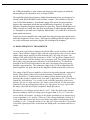
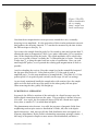
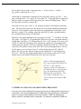
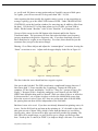
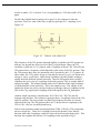
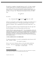
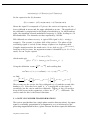
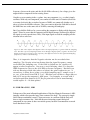
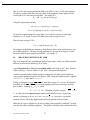
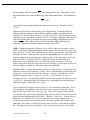
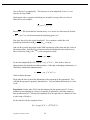
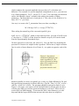
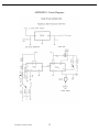
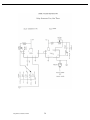
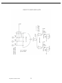
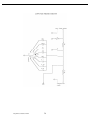
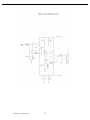
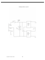
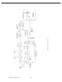
Physics 322, Physical Measurements Laboratory
Pulsed Nuclear Magnetic Resonance
(version February 2008)
I. INTRODUCTION
A. GENERAL COMMENTS
Nuclear Magnetic Resonance (NMR) spectroscopy is perhaps one of the most important
scientific developments of the twentieth century. Since its discovery in the mid 1940’s,
NMR has found applications ranging from solid state physics and materials science to
chemical analysis and biophysics. This experiment will serve as an introduction to many
of the chemical and physical principles underlying such studies. While many phenomena
can be explored with this apparatus, time may not allow for the completion of every
exercise. In performing the lab, then, be sure to choose a wide assortment of
measurements.
B. REFERENCES
Before proceeding, it is essential to become familiar with the theory and concepts
governing NMR. Particular emphasis should be given to understanding Boltzmann
equilibrium, the Larmor frequency, rotating reference frames, free precession, nutation by
radio frequency (RF) pulses, spin echoes, T1, T2, and chemical shifts. Note that without a
prior comprehension of these concepts, the lab will not be understood at all. The material
in this write-up does not substitute for reading the references.
The following publications are excellent references for this experiment:
i.
ii.
iii.
iv.
Experimental Pulse NMR: A Nuts and Bolts Approach, by E. Fukushima and
S.B.W. Roeder. A must-read for the basics, especially pp. 1-35, 50-60, 125-139,
185-197, and 297-312.
High Resolution Nuclear Magnetic Resonance, by J.A. Pople, W.G. Schneider,
and H.J. Bernstein. Specific attention should be given to Chapter 1 (pages 3-11),
Chapter 3 (pages 22-49), and pages 50-73 and 82-86 of Chapter 4. Chapter 5
presents a fairly light introduction to the high-resolution spectra used in chemical
analysis.
Concepts in Magnetic Resonance (John Wiley & Sons, Inc.) Vol. 12(5), 257-268
(2000). This article describes the apparatus and experiments of this laboratory
exercise.
There is a good NMR text on the web by U. Hornak at
http://www.cis.rit.edu/htbooks/nmr . Hornak has a companion text on MR
Last printed 3/10/08 3:41 PM
1
imaging at the same address (but htbooks/mri). The NMR text is available at the
Physics 322 website.
II. PULSED NMR APPARATUS: HARDWARE DESCRIPTION
The pulsed nuclear magnetic resonance apparatus used in this experiment is simple but
exhibits state-of-the-art performance. Its principal components include a 14,092 gauss
permanent magnet, an NMR probe, an RF receiver, an RF transmitter, and a pulse
generator; data analysis and spectra acquisition is performed using a PC. For reference, a
block diagram of the complete system along with circuit drawings of the probe, RF
receiver, RF transmitter, pulse generator, and power supply may be found in Appendix I.
The block diagram is must-reading; it is the last page of this write-up.
A. PERMANENT MAGNET
The permanent magnet used in this experiment is manufactured by Hitachi. Having a
field strength of 14,092 gauss, the magnet also obtains very high field homogeneity (i.e.,
field uniformity). In order to maintain field stability, the temperature of the magnet must
remain at 35 degrees Celsius. An inner, proportional oven and an outer (‘guard’) on-off
controller provide this regulation. The electronics for temperature control are at one end
of the magnet. The power consumption for the magnet is well under 100 watts. The field
strength determines the frequency of spin precession, which is here (for H nuclei at
14,092 Gauss) 60.00 MHz.
Note: The Hitachi unit has no on-off switch! Leave it plugged in at all times –
including the days and months of semester breaks - to keep the magnet at a stable
temperature.
To improve the field homogeneity, a set of electrical gradient coils (termed ‘shims’) are
provided. The shim coils are attached to the NMR probe – and thus are not within
viewing range. These coils do allow for gradients to be generated. A set of 9 controls on
the front panel of the magnet frame permits for adjustment of field homogeneity. The
most recent resonance settings have been logged in a red notebook labeled “NMR
Experiment,” kept with the apparatus. Fine tuning of these settings will cancel most
imperfections in the permanent magnet, thereby producing an extremely homogenous
field (to a few parts in 108).
i.
As the labeling of some of the controls suggests, each control adjusts a coefficient
in a three-dimensional Taylor expansion of the field strength:
H(x,y,z) = Ho + axx + ayy + azz + …
where ax is controlled by the knob labeled x, ay is controlled by the knob labeled
y, and az is controlled by the knob labeled z.
Last printed 3/10/08 3:41 PM
2
ii.
iii.
In addition, there is a (very) FINE Y control, which, as the name suggests, allows
for fine-tuning on Y. A FIELD SHIFT knob at the left allows the field to be
changed by 0 to 0.7 gauss (approximately, a 3000 Hz range), up or down
depending on the ± switch selection.
The power supply below the shim control panel is used to power both the shims
and the temperature controller board. It has 120 VAC at a few points, so keep
your hands out of it.
B. NMR PROBE
The NMR probe contains the RF coil* that surrounds the NMR sample, used for both
transmitting (i.e., flipping the spins) and receiving (i.e., detecting the precessing spins.
This is accomplished by conversion of the precessing spin magnetization into a radiofrequency voltage). For greater efficiency, the coil is tuned by appropriate capacitors to
60 MHz. The impedance of the coil is transformed to be 50 ohm resistive, the industry
standard value for radio-frequency equipment.
The NMR probe may be thought of as a transducer, converting between the realm of RF
voltages and currents and the realm of RF magnetic fields. Loosely interpreted, then, the
NMR probe may be considered as an antenna; note however that none of the energy is
actually radiated.
For experiments requiring an extremely homogeneous field, the sample tube can be
rapidly rotated such that each spin will more nearly feel the same time-averaged field
strength. That is, each spin will spend time in regions of higher and lower field strength,
so an averaging occurs. For this purpose, an air jet and air turbine wheel are used. While
Hitachi originally used a small compressor to generate the air for the jet, this approach
was abandoned in the Physical Measurements Lab. Rather, house air is used instead: a
regulator in the Lab is permanently set to +3 psig (equivalently, 0.2 atm positive
pressure). This air is connected via hoses to the barb fitting of a valve located on the
front-left side of the magnet’s frame. The amount of air flow into the probe may be
controlled by this valve. The spinner can be temperamental; Hitachi chose their design to
avoid the competitor’s superior, patented design!
C. RADIO-FREQUENCY RECEIVER
As seen in the system block diagram, the spin signal from the NMR probe is directed by
the diode boxes to the Hitachi amplifier (51 dB gain, 60±1 MHz). The input amplifier is
low-noise, as is appropriate for 10-100 microvolt signals. The signal is passed to an
additional 32 dB gain amplifier through a step attenuator (0-31 dB in 1 dB step
increments), which allows the overall gain to be reduced for large signals. The output of
*
Note that the RF coil has about a 5.5 mm diameter and is about 2mm long – a very short solenoid. This is
why the field H1 is so inhomogeneous, even across small volume samples.
Last printed 3/10/08 3:41 PM
3
the 32 dB gain amplifier is at the Larmor spin frequency (the frequency at which the
nuclear spins precess about their axis), or nearly 60 MHz.
The amplified signal is then frequency-shifted (heterodyned) to near zero frequency by
mixing it with the 60.000 MHz crystal oscillator’s output. (This oscillator is also the
source of the RF transmitter.) Note that the output of the mixer (the phase-sensitive
detector) has components at both the sum and difference frequencies. It is only the
difference frequency that passes through the low-pass filter. Thus the NMR signal at 60
MHz ± (where is small, since the spins are quite near 60 MHz) appears at frequency
. This signal is of a much lower frequency than 60 MHz. See section III L for more on
phase-sensitive detection.
In brief, the receiver amplifies the weak signals from the precessing spins and the mixer
shifts their frequencies to low values. This frequency shifting makes the signal easier to
see on the oscilloscope and easier to digitize for recording in the computer.
D. RADIO-FREQUENCY TRANSMITTER
As seen in the system block diagram, the 60.000 MHz crystal oscillator is the RF
source. The oscillator's output is split, with one output going to the receiver's mixer
and the other output gated by Hewlett-Packard gates. By using two gates, any
leakage of RF pulses while the transmitter is in the "off" position is suppressed (if
the first gate doesn’t kill the leakage, the second gate will). The gating signals for
these gates come from the pulse generator (as described below). To control the
strength of the RF field Hl presented to the spins, the output of the gates passes
through a step attenuator. The attenuator output feeds a 10 Watt (maximum) RF
power amplifier; the gain control on this amplifier should remain fully clockwise.
The output of the RF power amplifier is directed to the probe through a network of
diodes. These diodes collectively form the automatic Transmit-Receive (T-R)
switch. Recall the V-I characteristics of ordinary silicon diodes: in the forward
direction, the current I remains nearly zero until V approaches 0.5-0.7 Volts (this is
termed the ‘forward knee’). As a result, a pair of diodes in parallel with reverse
polarity will act as a high impedance for small signals (like the 10-100 microvolts
generated by the precessing spins) and as a low impedance for large signals (like
the many volts from the RF power amplifier during RF pulses).
Put otherwise, for voltages greater than 0.5 to 0.7 Volts, the diode in the forward
direction conducts, while for voltages more negative than -0.5 to -0.7 Volts, the
reverse diode will conduct. In doing so, the diodes essentially act as shorted wires
or zero impedance (‘on’ switch). However, if the voltage magnitude is below |0.5|
Volts, neither the forward nor the reverse diode can conduct, rendering the diode
assembly as ‘off’. Using this model of ‘on’ and ‘off’ silicon switches, it is possible
to track the signal/power flow to and from the NMR probe, in transmit and receive
modes.
Last printed 3/10/08 3:41 PM
4
In the event that a transmitter pulse of excessive amplitude and/or duration is sent to
the NMR probe, the fuse should blow before the diodes and the NMR probe are
damaged (see block diagram). Because the pulse generator can put out long pulses
when it is turned on or off, the RF power amplifier should always be turned on
last and turned off first. In this way no long pulses are sent to the probe.
In summary, the RF transmitter generates RF pulses (as commanded by the pulse
generator) to produce the RF magnetic field H l in the NMR probe; it is this timevarying field that flips the spins. A network of diodes performs automatic T-R
switching, allowing the same probe to be used for both transmitting and receiving.
E. PULSE GENERATOR
The pulse generator controls both the length of the RF pulses and the spacing
between them. The output of the pulse generator drives the transmitter gates and
triggers the oscilloscope and/or computer used to display and/or acquire the spin
signal.
This is a simple pulse generator that runs a fixed sequence. The sequence is initiated
by the repetition rate generator, which sends out a triggering pulse every 0.1-100
seconds (as selected by front panel knobs). This triggers pulse 1 followed by a first
delay, then pulse 2 followed by a second delay, and then pulse 3. The entire
sequence repeats with the next triggering pulse as demanded by the repetition rate
generator. Note that the pulse widths can be independently adjusted from 1-100 μsec
and the delays can be set independently from 0.1 msec to 10 seconds.
Each pulse (1, 2, and 3) has a separate front panel output BNC port for triggering
either the counter/timer, the oscilloscope or the computer at the desired point in the
pulse sequence. The output to the transmitter gates is toggle-switch selected to
include pulse 1 (off-on), pulse 2 (off-on), and pulse 3 (off-on). Turning a pulse off
at the toggle switch does not change the internal workings of the pulse generator;
rather, the deselected pulse simply is not sent to the transmitter gates. So, for
example, one could still trigger on pulse 2, even if only pulses 1 and 3 are sent to
the transmitter gates.
F. OSCILLOSCOPE
The Tektronix 2221A oscilloscope is a storage device allowing for real-time
acquisition and analysis of NMR signals. To begin, select “non-storage” and use
it as an ordinary scope. Start with a liquid sample, 2 ms/cm time-base, 20 mV/cm
vertical base and external triggering; one trace per pulse will be generated.
For a non-blinking (stored) display, hit the "storage" button. Note that the scope
has separate intensity controls for store and non-store. Throughout most of this
experiment, the scope should remain in the ‘stored’ display. (You'll really
Last printed 3/10/08 3:41 PM
5
appreciate the storage feature - it's a lot easier to look at.) In the event the scope
is not set up for storage, hit the ACQ button in the SETUP box. Hit the 4K/1K
button and turn the cursor knob until “Trig Pos: 4K/1K” appears. Now hit ACQ to
exit; the scope should be set to store.
Note that the Tektronix 2221A is a lot more oscilloscope than will be needed in
this experiment. Once set up though, its extra capabilities do not get in the way.
G. COUNTER
The Hewlett-Packard 5314A is a 100MHz/100ns Universal Counter. It features a sevendigit, seven-segment LED display with overflow indication, seven function performance,
and full input signal conditioning. The seven functions of the counter include Frequency,
Single-Shot Period, Period Average, Time Interval, Totalize, Ratio, and Self Check.
These functions are accomplished by a single LSI integrated circuit. The input signal is
AC coupled and can be conditioned by slope selection, trigger level, or attenuation.1
Throughout this experiment, the counter will be used to achieve enhanced accuracy in
setting the pulse width and measuring pulse delays. Only the four buttons to the right of
the counter should be adjusted.
In adjusting the counter settings, the objective is to trigger to start the timer on the front
edge of the pulse and stop the timer on the back edge. The ‘+/- slope’ switch controls
whether the ‘event’ occurs when the input voltage goes up or down through the selected
level. The level control is responsible for generating an event when the input signal
passes the dialed-in level (DC voltage) in the direction given by the slope (+/-).
There are 2 events: one to start the counter and the other to stop. You can choose to start
and stop on the same voltage source or 2 different sources (a setting marked ‘SEP’ for
separate inputs or ‘COMMON’ for a single input). On ‘SEP,’ you could choose to
measure the time interval between the + (rising) edge of a voltage input into the A BNC
connector and stop on the - edge of the voltage hooked to the B BNC connector, or,
conversely, you could choose to measure the interval starting on the – edge of the A input
and stopping on the + edge of the B input. On ‘COMMON,’ you can time the interval
from one edge to the other of the same voltage (input to A; no choice, it must be A).
So to measure the length of (say) pulse 1, hook the “output 1” of the pulse generator to
the timer’s A input. The slope settings should be + and – (left, right) and you should
select COMMON.
To measure the delay between pulses 1 and 2, hook “output 1” to the timer’s A input and
“output 2” to B input. Select “SEP” (for separate). The delays are generally much longer
1
As adopted from the HP 5314A Universal Counter Operating and Service Manual. For additional
information, please refer to this manual, located on the table next to the magnet. The manual is also
available from the 322 class web-site.
Last printed 3/10/08 3:41 PM
6
than the pulses themselves, so it matters little whether you trigger on pulse 1’s rising or
falling edge (same with pulse 2).
Use the N=1 setting (no averaging) and select time interval A to B (TI, A-B). The shift
key (black/blue) should be on blue. The timer counts in microseconds. Leave the two
level knobs pointing to the + symbol (this is in the middle of the TTL voltage range of 0
to 3 volts).
H. COMPUTER
The computer can be used to digitize, signal average, and/or store any signal viewed by
the oscilloscope. The Pentium 4 PC supports a Windows XP operating system. It has a
processing speed of 1.6GHz and a memory of 128MB RAM. FIDoLite* software,
developed by Caleb Browning and Sam Gross of Mark Conradi’s research group, allows
one to acquire and save signal data and launch the signal analysis. FIDoLite may be
accessed either from the Desktop or from the shortcut in the Start Menu.
Once the program has opened, two displays can be seen on the screen. If a sample is in
the probe, hit “Acquire.” The top display will output the signal seen on the oscilloscope
while the bottom display will be zeroed out. This bottom graph is a remnant from the full
FIDo program and is not used in this experiment. Your hardware has a single phase
detector, with its output representing the spin magnetization along a particular axis in the
rotating frame. The software supports two phase detectors (called in-phase and
quadrature, I and Q,) along perpendicular axes in the rotating frame.
Before acquiring signal, make sure that the data directory is set to c:\FIDo\data\. Once
signal has been acquired, be sure to save the data in the ‘data filename’ slot. All
filenames should end with the file extension ‘.dat’.
The upper-limit, lower-limit control adjusts the maximum and minimum voltage levels
displayed on the graphs. Note that the digitizer saturates at a ±5 Volts regardless of the
value of these controls. To ensure that the signal is not clipped by exceeding the
digitizer’s input range, the receiver attenuation should be set such the FID fits within
±2.5 Volts on the display.
The trigger level value controls the voltage required to trigger the digitizer. The trigger
signal is TTL (transistor-transistor logic); thus you should use the default value of 1.6
Volts.
The trigger slope function determines whether the digitizer will trigger on the rising
(positive) edge of the signal or the falling (negative) edge. This should remain in its
default position of triggering on the negative (falling) edge.
FIDoLite also allows the user to set the dwell time (the amount of time between
successive time points), the number of points (how many points will be sampled each
*
Note that Dr. Conradi’s group plans to maintain FIDoLite for its research
Last printed 3/10/08 3:41 PM
7
acquisition), and the number of acquisitions. The phase, which determines what angle (in
degrees) the incoming data will be phase-shifted, can also be adjusted. This value should
remain at its default position of zero degrees.
Note that Fourier analysis is easily and quickly performed by depressing the ‘analyze’
button. Once in the analyze screen, hit ‘Fourier Transform’ to acquire the FFT spectrum.
Please see section III F for more details.
For additional information regarding the FIDoLite program, a FIDoLite User’s Manual is
included on the Desktop. In the event of program failure, a backup floppy disc is
available. A copy of the backup disc may be obtained either from the teaching team or
from Conradi’s group.
IMPORTANT CONSIDERATIONS
1. Hardware Do’s and Don’ts
i.
ii.
iii.
iv.
v.
Always leave the Hitachi unit plugged in.
Do not break a sample tube in the probe. Insert and remove sample tubes
with the greatest caution. If you do break one, don’t make it worse – get
help.
Do not let foreign objects fall into the magnet’s opening. Be sure to keep the
opening covered by the Plexiglas fitting at all times.
Besides the shim controls, do not adjust the magnet. Receive help if it
doesn’t seem to be working.
Always turn on the RF power amplifier LAST. Turn this unit off first. In
fact, we recommend turning on and off only the power amplifier,
oscilloscope, and counter/timer. The rest of the apparatus should remain on.
2. Depth Gauges
i.
ii.
iii.
Two depth gauges are provided with the wooden sample tube holder; made of
Plexiglas, these gauges allow you to insert the NMR tube and adjust the height of
the air turbine wheel.
In the longer depth gauge, the distance from tube bottom to the bottom of the air
turbine is 103 mm. This setting will be used in spinning the sample tubes. At this
setting, the glass tube spins with its weight supported by a little Teflon disk
(bearing) at the bottom of the probe. The turbine wheel stands free, so it can spin
the tube.
The shorter gauge is set for 89 mm, and is used for holding the bottom of the
NMR tube near the center of the RF coil. This setting is handy for putting small
amounts of sample into the RF coil. Note the weight of the tube rests on the
turbine, so it will not spin this way; leave the spinning-air off.
III. PROTON NMR EXPERIMENTS
Last printed 3/10/08 3:41 PM
8
A. SETTING UP – FINDING A FIRST NMR SIGNAL
Insert a sample of water into the probe and set the receiver attenuator to 16 dB
(towards the ‘in’ direction) of attenuation and the transmitter attenuator to 13 dB.
Use the 103 mm depth gauge so that this long sample extends both above and
below the RF coil. The oscilloscope should be on a 5 ms/cm time-base and a 20
mV/cm vertical setting. Ensure that the vertical input of the oscilloscope is
connected to the unamplified output of the low-pass filter box.
The oscilloscope should remain on 20 mV/cm. If the signal is too large or too
small, change the receiver attenuator accordingly. Note, if the attenuator switch is
“IN”, this means the decibels (dB) of attenuation are in the signal path (so,
attenuating). If the switch is “OUT”, the attenuator is out of the path (so, no
attenuation). The total attenuation in dB is the sum of all the “IN” sections.
Decibels:
PIN
). So 10 dB is a power ratio of 0.1 and
The number of dB = 10 log ( POUT
10
voltage ratio of 1 / 10 (because power is proportional to voltage squared).
dB________P-ratio________V-ratio
0
1
1
3
2
1.414
6
4
2
10
10
3.16
20
100
10
30
1000
31.6
46
40000
200
Set the pulse generator for a repetition rate of one pulse per second; input a single
pulse (make it pulse 1) of about 2 μsec width. Note the knobs on the pulse
generator have scales for approximate reading. The oscilloscope should trigger
externally (external trigger source) on pulse 1.
You should see an NMR signal! To acclimate yourself with the electronics, you
may want to spend some time “flying” the controls. Vary the receiver attenuation.
Make the pulse width shorter and longer. Adjust the field shift control on the
Hitachi shim panel; you should be able to make the displayed signal pass through
zero frequency (“zero beat”). Recall the oscilloscope sees the phase detector output,
which is the difference frequency between the spins and the 60.0 MHz oscillator.
Try turning the shim controls to see how an inhomogeneous field leads to a more
rapid decay (shorter time duration, T2*) of the signal’s envelope. This free
induction decay may be visualized in the following way:
Last printed 3/10/08 3:41 PM
9
Figure 1: The FID,
both as visualized in
the x-y rotating
frame, and as seen
on the oscilloscope.
Note that the net magnetization vector precesses around the z axis, eventually
decaying to zero amplitude. It is the projection of this circular motion onto one axis
that produces the decaying sinusoid. T2 * can thus be measured by the time it takes
the FID envelope to decay by 1/e.
Now remove the sample from the probe for 10 seconds (a time much greater than T1,
allowing the spins to demagnetize). With 1 μsec pulse width and a 0.4 sec repetition
time, let the sample back into the probe. The signal amplitude will be observed to
grow over a period of about 2 seconds, the T1 (relaxation time) of water. Note that
it takes time T1 to bring the spins back into a state of equilibrium. Here you used
small-angle RF pulses, so as to perturb the relaxing spin magnetization as little as
possible.
Avoid overloading the receiver. Keep the output level at the unamplified output of
the low-pass filter below 0.1 Volts peak-to-peak (2.5 Volts peak to peak at
amplified port). Use the step attenuator to accomplish this. This limit of 0.1 Volts
peak-to-peak is 5 cm peak-to-peak vertically on the scope (20 mV/cm setting).
As previously mentioned, handle the sample tubes with caution: Once the sample
tubes are in the hole at the top of the probe let the tubes gently fall into place.
When removing the tube, gently lift straight up.
B. MOTIONAL AVERAGING
In general, the diffusive motions of the molecules in a liquid average away the
dipole-dipole interactions between the spins. This averaging is absent, however,
in a solid. As a result, the free induction decay (FID) has a much more rapid
decay time (a smaller T 2*) in solids than in liquids.
The phenomenon arises because, in a solid, the presence of magnetic fields from
neighboring nuclear spins causes a distribution of fields, H; this is the dipoledipole interaction. And, since =H, this field distribution also corresponds to a
frequency distribution. By the Fourier relationship (uncertainty principle) t 1,
this range of frequencies implies a more narrow time distribution, and hence a
Last printed 3/10/08 3:41 PM
10
shorter T2 *. Let’s say it differently: assume a set of spins or oscillators with
frequencies distributed over a range . At t=0, they are all in-phase. It takes a
time T2 * for them to get appreciately out of phase (maybe 1 or 2 radians), with T 2 *
= 1/.
Use a single pulse of 2 μsec width repeating every 2 seconds. You do not
need to spin these samples. Compare the free induction decays of the
following:
i.
ii.
iii.
iv.
v.
vi.
Water
Adamantane – an organic solid where the molecules rotate freely but
do not translate; C10H16, a tetrahedral shaped molecule.
Plexiglas – a very rigid solid with essentially no motions; polymethylmethacrylate
Rubber – which, according to NMR, seems more like a liquid than a
solid
Grease – also liquid-like, a swollen gel
You could also study the curing of a 2-part epoxy. Just mix the two
parts together and place a small amount in the bottom of a 5mm
NMR tube (make sure none gets on the outside of your tube!). Use
the air turbine to hold the end of the tube near the RF coil. The
89mm depth gauge will help to achieve this end. As the epoxy
cures, T 2* should get shorter (the material becomes increasingly
solid-like). Use “5-minute” epoxy and work fast so you don’t waste
a whole day doing this!.
In each case, it is the length of the decay (T2 *) in which we are interested. Note
that the T2 * of the above solids is on the order of 10-100 μ sec, while the T2 * of
water is limited by the magnet’s homogeneity and is approximately 20 msec here.
(This factor of 1000 is big!)
When looking at the rapidly decaying signals of solids, be sure to use a short filter
time constant (1 or 2 μ sec). To guarantee that you are seeing NMR (and not just the
tuned circuit ringing of the probe), try removing the sample to see the difference.
Since the Hitachi-built probe has some hydrogen-bearing solids near the coil, there
is a signal with a short T2 * even without a sample inserted, but it will be smaller
than the signal of the plexiglass. You can convince yourself that you are seeing the
plexiglass NMR signal by watching on the oscilloscope for the displayed signal to
increase when you drop-in the plexiglass sample tube.
C. NUTATIONS
The experimental objective in studying nutations is to examine the effect of an
RF pulse upon the spins. A single pulse is applied to the sample with a
repetition time much greater than T 1 . In this way, the spins are allowed to
return to equilibrium before another pulse of magnitude H 1 is applied for a
time t (the width of the pulse). The spins are expected to nutate (or
Last printed 3/10/08 3:41 PM
11
precess) about H 1 through an angle of H 1 t =. Since the spin’s
magnetization M starts along the z-axis, the projection of M in the x-y plane
will be:
M o sin = M o sin(H 1 t )
From the variation of amplitude with t , one can determine both the nutation
frequency H 1 /2 (where /2 = 4.2577 x 10 3 Hz/gauss for protons) and the
pulse widths that correspond to 90 and 180 degree pulses. You will
recognize a 90 degree pulse as the pulse giving maximum FID amplitude; the
180 degree pulse produces a minimum amplitude FID following it. Note that
a plot of M versus t will produce a damped sinusoidal oscillation. Plot this
for yourself. The damping is due to the variation of H 1 over the sample
volume. Recall the RF coil is quite small, so its field H 1 is not very uniform.
For this experiment, use the sample of glycerol (which has a very short, convenient
Tl of about 0.1 sec). The amount of glycerol in the sample tube is fairly small,
allowing all the spins to more nearly see the same Hl. Using the air turbine, suspend
the sample tube so that the sample is close to the center of the probe’s RF coil; from
the bottom of the turbine to the bottom of the test tube should be 89 mm (the 89 mm
depth gauge should be used to obtain this distance). Use a single pulse, repeating
every 1.0 sec (>> Tl ). Record the initial amplitude of the spin signal versus t of
the pulse. Pulse width should be measured using either the oscilloscope (or a
second oscilloscope) or the counter-timer. To measure the signal amplitude, be sure
to get off resonance enough to provide a convenient beat note whose amplitude is
easily determined. Use the field shift knob to get an FID similar to that of Figure 1.
Note that by looking at the initial phase of the signal, it is possible to distinguish
between + and – amplitudes. This is easier if you are closer to resonance, since here
there are fewer beats in the FID.
It is advisable to determine Hl for 3 settings of the transmitter attenuator. Keep the
results handy so you can set 90° and 180° pulses for many of the later exercises.
D. SPIN ECHOES AND T2 MEASUREMENT
Spin echoes are an interesting phenomenon, demonstrating that spectroscopic
techniques can modify the system Hamiltonian. In the spin echo, the 180 degree pulse
positions the spins as though they ran backwards between the two pulses.
A spin echo is formed using a two pulse sequence, consisting of a 90° pulse
followed by a delay and then a 180° pulse. If the net magnetization vector is
assumed to be initially oriented along the z-axis, the /2 pulse (along x) will rotate
the magnetization by 90 degrees to the -y-axis. During time between the first and
second pulse, the different spin packets will freely evolve (or dephase) in the x-y
plane because they see slightly different static fields H and precess at slightly
different frequencies = H. The pulse then rotates each magnetization vector
Last printed 3/10/08 3:41 PM
12
180° about the x-axis of the rotating frame, leaving the vectors again in the x-y
plane. After a further time , the magnetization vectors are back in phase along the
y-axis and an echo is observed (see Experimental Pulse NMR: A Nuts and Bolts
Approach for a good discussion complete with figures).
In this exercise, the behavior of the spin echo will be used to determine T 2 of
glycerol. Use the depth gauge and put the short sample of glycerol in the probe at
the correct height (89 mm). Select two pulses set to 90° (pulse 1) and 180° (pulse
2). Space the pulses by = 5 msec, say, to start. Un-adjust the shim controls to
make a rapid decay (short T 2 *), easily achieved by mis-adjusting the z-shim by a
couple of turns on the knob. Don’t forget to record the “correct” setting so you can
return to it. Tune onto resonance (use field shift knob) so a rapidly decaying FID is
seen after pulse 1 and you will see a similar but inverted spin echo at time after the
second pulse. Use 1.0 sec repetition time and trigger on the first pulse.
You should see an FID after pulse 1, possibly a weak FID after pulse 2, and a spin
echo at 2 after the first pulse. Try varying the spacing to see that the echo really
does occur at time 2 (measuring from the first pulse). For fixed vary the first
and second pulse widths to obtain maximum echo amplitudes. These pulse widths
should correspond to 90° and 180° nutations, as found in part C. Plot the echo
amplitude M on a log scale as a function of 2. A nearly exponential decay obeying
Ae-2 /T2 will be observed. Determine T2 of glycerol.
You can use linear graph paper to plot log M as a function of 2. If M is the echo
amplitude and
M = exp(2/2), then
Ln M = ln A –(2)( T12 ). This is of slope –intercept form, y = b + mx,
where y = ln M, x = 2 and the slope m = -1/T2 .
Likewise, the three-pulse sequence /2- - /2-T- /2- -echo (with T > ) creates
a stimulated echo at time after the third /2 pulse. Again it is assumed that the net
magnetization vector is initially oriented along the z-axis. This equilibrium zmagnetization is transferred to transverse magnetization by the first /2 pulse.
During free evolution of length , the magnetization dephases. The second /2
pulse rotates the magnetization vectors into the xz plane. During time T, the
transverse magnetization decays, while Mz stays constant (no precession since it is
parallel to the field). At time t = T + , the third /2 pulse transfers the zmagnetization pattern again to transverse magnetization which forms an echo at
time t = T + 2 along the +y-axis.
Roughly speaking, the /2- - /2-T- /2- -echo sequence is a 90- -180- -echo
where the 180 is broken into two 90° pieces spaced by T. During this “time-out,”
the spin magnetization component parallel to z does not precess, so that the interval
T does not affect the echo formation: Try varying the delay intervals and see if you
Last printed 3/10/08 3:41 PM
13
can identify all the FIDs and echoes you see. We recommend the three pulses be
45, 45, and 90 degrees, to best see all the echoes. Try turning off one or more of the
RF pulses (toggle switches on the pulse generator) to check yourself-the 1-3 echo
(FID following pulse 1 refocused by pulse 3) will not disappear when pulse 2 is
switched off, though the 1-3 echo may change amplitude. When pulse 1 is off, you
will see an echo of the FID following pulse 2, refocused by pulse 3. It may help to
keep these echoes apart from each other in time. We recommend using a first delay
of 5 ms and a second delay of 15 ms. You may need to reduce the field uniformity
(z shim knob) so the FIDs and echoes are short and do not run into each other.
E. MEASURE RELAXATION TIME T1
This exercise will allow you to measure the spin relaxation time T 1 - i.e., the time it
takes the system to return to equilibrium – using two distinct methods: SaturationRecovery and Inversion-Recovery. Measure T1 for any of the following samples:
i.
Glycerol
ii.
Rubber
iii.
Grease
iv.
Solid Adamantane
v.
A solution of water with dilute cupric ion (paramagnetic). Note that the T1
of any substance is shortened by the large magnetic moment of paramagnetic
ions. Paramagnetic here means that the ion has a net unpaired electron spin.
In most substances, all the election spins are paired anti-parallel, leading to
cancellation.
Saturation uses a two-pulse sequence consisting of a 90° pulse followed by a delay t
and then another 90° pulse (90°-t-90°). The FID following the second “inspection”
pulse is proportional to the z-magnetization (Mz ) just before the pulse. Thus by
measuring the amplitude of the FID following this pulse, we inspect the Zmagnetization just prior to the pulse. In order for the FID to decay rapidly (to
prevent one FID from running into the next), the z-shim may be un-adjusted.
Trigger the scope on the second 90° pulse so that the FID from pulse 2 is observed.
Both pulse 1 and pulse 2 should be switched on at the pulse generator.
Vary the time t using the first delay’s knobs; watch the FID amplitude change as
you do. The FID signal amplitude M will vary as
M(t) =A (1-B exp (-t/T1 )).
For a perfect first 90° pulse, B=1.
If t >> T1 (this t can be regarded as infinite), M=A so
M – M(t) = AB exp(-t/T1 ). Taking the natural log of both sides,
Ln [M - M(t)] = ln (AB) + (-1/T1 ) t.
Last printed 3/10/08 3:41 PM
14
We recognize this as slope –intercept form, y = b+mx, where y = ln [M –
M(t) ] and x=t and slope m=(-1/T1 ).
Notice that it is important to measure M for a long delay time to get “M ”. You
may recall that for t > 5T1, exp(-t/1 ) is less than 1%. You might also be impressed
that our analysis in terms of the slope makes the value of B unimportant. That is,
the first pulse need not be exactly 90°.
Inversion recovery uses a 180°- t -90° (inspect) sequence to determine relaxation
time. The first pulse inverts Mz; Mz then recovers towards equilibrium during the
interval t. The second 90° pulse tips whatever magnetization is along the z-axis
into the x-y plane. The resulting signal just after the 90° pulse is proportional to
the z-magnetization just prior to the pulse.
Therefore, the signal amplitude will vary again as A(1-Be - t /T1 ), with B=2 for ideal
180° pulse. See Figure 2. By plotting M-M(t) on a log scale, one again obtains a
straight line with slope -1/Tl. When using the 180°- t -90° sequence, be sure to wait
at least 5T1 between repetitions of the experiment. Otherwise, the magnetization
coming into the sequence will be less than the equilibrium value M. That is, you
want your 180° pulse to work on the full, 100% recovered magnetization. So you
let the spins recover (at least 5 times T1 ) before doing the next 180° and 90°
pulses. By the way, this tedious waiting is not required for T 1 measurement by
90°-t-90°. After all, any magnetization that recovers between the one 90°-t-90°
and the next is just slated for death (Mz =0) by the next 90° pulse.
Figure 2: How the magnetization
Mz varies just after the 90°pulse in
the 180°- t -90° (inspect)
sequence (solid curve) and 90°-t90° (dashed curve). The plot also
gives the amplitude of the FID
following the second pulse. The
role of the second pulse is to
convert Mz into observable NMR
signal.
F. CHEMICAL USES OF NUCLEAR MAGNETIC RESONANCE
In recent years, Nuclear Magnetic Resonance has become an indispensable analytical tool
in chemistry. The chemical applications of NMR range from analyzing the content and
purity of a sample to determining its molecular structure. NMR can quantitatively
analyze mixtures containing known compounds. For unknown compounds, NMR can
Last printed 3/10/08 3:41 PM
15
either be used to match against known spectral collections (tabulated in books or on-line)
or to infer the molecular structure directly. Once the basic structure is known, NMR can
be used to determine molecular conformation in solution; it can also be used to study
physical properties at the molecular level, including conformational exchange, phase
changes, solubility, and diffusion.
We note, for example, that the Washington University Chemistry Department has
approximately 4 NMR machines for analysis of reaction products. This translates into a
2 million dollar investment. Nationwide, the monetary total of all NMR instruments is
perhaps 1 billion dollars (!).
This exercise will lead you through the basics of chemical NMR spectroscopy.
So how does chemical NMR spectroscopy work? Consider for example a simple (and
perhaps all-too-familiar) molecule: CH3CH2OH, ethanol. This compound has three types
of hydrogen nuclei including CH3 (methyl), CH2(methylene), and OH (hydroxyl). For
each of these, the resonance frequency is proportional to the field Hn at the nucleus:
f = (/2)Hn
And the field at the nucleus H n is made up of the external field H o from the
magnet and a weak field from the nearby electrons:
f = (/2) (Ho + H)
Now H is due to weak currents in the electronic cloud induced by the external field
(similar to eddy currents). So, H is proportional to Ho:
H = -
Ho
Note that the negative sign is incorporated into the definition by convention. Thus,
f = Ho(1- ) / 2
Here, is called the chemical shift; for protons, the range of chemical shifts is about 0-10
parts per million. These shifts are small!!!! NMR was around for a few years before the
shifts were observed. Basically, the early magnets were not uniform in field, so the NMR
lines were too broad.
However – and here’s the good part – even though is small, is different for each type
of hydrogen nuclei. Thus, in the same external field Ho, the CH3, CH2, and OH protons
(hydrogen nuclei) have three slightly different frequencies. The Fourier spectrum should
look like:
Last printed 3/10/08 3:41 PM
16
Figure 3: From left to right the
peaks with increasing frequency
are CH3, CH2, and OH, with the
intensity ratio 3:2:1 (ratio of
areas in the spectrum) arising
from the relative numbers of each
kind of proton.
Note that for ethanol, the overall width of the spectrum is about 4 parts per million. At a
60 MHz frequency, this implies that the spectrum is only approximately 240 Hz wide. If
the field Ho is not extremely homogeneous (ppm or better), then each line will be so
broad that it merges with the next. This is why it is of utmost importance to have a
uniform field.
Let’s get started. To shim (i.e., improve the homogeneity of) the magnet, use a single
pulse of about 1μsec every 0.5 seconds. Use a transmitter attenuation of 13dB. Such
settings correspond to a small tip angle so that the experiment can be repeated faster than
once per T l . More formally, the small pulse barely perturbs the magnetization
because the cosine of a small angle is nearly 1. Use the water sample,
suspended in the probe a distance of 103 mm (use the depth gauge). As will be
seen, the water sample has only a single resonance line; all the H nuclei are
equivalent.
G. SHIMMING
By adjusting the shim controls, you can make the water FID extend further
across the oscilloscope screen to the right (longer T 2 * means better field
uniformity as it takes longer to de-phase when the spins all run at more nearly
the same frequency). Start with the settings in the logbook, or the settings
from the last group of students (assuming they were successful).
Initial adjustment is done on x, y, and z with the sample tube not spinning. Go over
these in a loop 3 times. Now turn on the spinner-drive air and make sure the
sample is indeed spinning. With the sample of water spinning smoothly (in
truth, the spinner turbine and bearing are the least robust parts of the
apparatus; be forgiving), and having already set x, y, and z on the nonspinning sample, the important controls are y (or fine y) and curvature (with
the uninformative label “B”). Maximize the duration of the FID using fine y;
then try a new setting of B by 10 or 20 points (i.e., 0.1 or 0.2 turns on the
knob), again optimizing fine y.
With y (or fine y) and B adjustments, you should be able to make the water
FID last 0.5 seconds or so, with a 1/e decay time of perhaps 0.2 seconds,
corresponding to a frequency width (see below) of about 2 Hz. 2 Hz out of 60
MHz means the field is uniform to about 3 parts in 10 8 , which is remarkable.
Last printed 3/10/08 3:41 PM
17
Note: as you make the field more uniform and the FID grows longer in
duration, you will want to increase the repetition time, so that one FID is fully
decayed before you hit the next rf pulse. This might mean 1 pulse every 3
seconds. Patience is suggested.
Make sure to record your settings in the log book, to help keep track of
changes (it helps the next group of students). And if you turn the wrong
knob, you’ll be glad to have recorded the optimum settings, so your error is
easily corrected.
Figure 4: This figure
depicts the full width at
half maximum (FWHM) of
a resonance line.
You can now use the FIDoLite software to capture the FID and perform a FFT on the
FID, outputting the Real and Imaginary parts each as a function of frequency. Be sure to
save the FID and the final Real and Imaginary FFT files with the extension ‘.dat.’ To
view and print the files, you can access the data arrays from EXCEL. First, from EXCEL,
open the directory the data is saved in (should be c:\FIDo\data\). Then choose file type as
delimited, hit ‘next’, and set delimiters as tab. The worksheet will display all numerical
values associated with the signal and spectrum. To graph the data, simply create a new
chart in the EXCEL worksheet.
Acquire one FID (no averaging needed-these are big signals) and Fourier transform
(FT) it - you'll see a single line because H2O has all equivalent hydrogens. (Your FT
software package cannot distinguish + and - frequencies, so the spectrum will have
mirror symmetry about the origin). And there may be an even bigger line at zero
frequency if you did not correct the baseline of the data.
How to FT: Now is a good time to teach you how to FT properly. First, choose a
dwell time (DW, time per point) which is short enough that you properly sample the
highest frequency component of the signal (look at FID on scope). The Nyquist
criterion is that the highest frequency sine (or cosine) needs at least 2 samples in
each cycle. Typically, the dwell might be 100 s to 1 ms.
Next choose the number of acquired points N so that the total time duration T of the
acquired data set is long enough to fully capture the signal; the signal should decay
fully in the first ~30% of the time. T determines the “digital frequency resolution”,
with the frequency-domain points (i.e., after Fourier transformation) spaced by 1/T.
Let’s say you want 0.25 Hz spacing in frequency, so your time-domain data set must
be T~4 seconds long. At a dwell DW = 1 ms, this is N=4000 points (FIDo knows
2n, so it will make this N=4096), a manageable data set. But if you chose DW=10
Last printed 3/10/08 3:41 PM
18
s, you’d need 100 times as many points and you’d quickly run out of disk space.
As a guide, you will never need N to be greater than 16K = 16,384.
After acquiring the data (usually the signal-to-noise is great, so one acquisition or
average is plenty), go to the ANALYZE feature of FIDo. Under TRANSLATION
CONTROLS, put-in the baseline window (for removing any dc additive offset from
the data). Use the last 25% of the data points (so for N=4096, go from 3000 to
4000). Hit the button “Baseline” to do it; here “Baseline” is an imperative verb.
Get out of this screen (use the OK button at the bottom) and hit the Fourier
Transform button. The spectrum will show lines mirrored about zero frequency;
just pay attention to the positive frequency side. If you have baselined correctly,
there should not be a spike at zero frequency. For water, there should be just one
resonance line (except for the mirror image).
Phasing: Go to Phase Adjust and adjust the “constant phase” correction, leaving the
“linear” correction at zero. Adjust until the upper display looks like in Figure 4.1.
Figure 4.1
Phasing of lineshape.
The idea is that the curve should not have negative regions.
Now put in ethyl alcohol. The FID is much more complicated because there are 3
lines (more than 3, if one considers the J-couplings). Capture the FID in the
computer, FT the signal, and display. You'll see 3 lines (or 3 groups of lines), like
Figure 3. Because of the ± frequency ambiguity, you'll want to use the FIELD
SHIFT knob (Hitachi shim panel) so that all 3 lines are either all above or all below
0 (this means the 3 sets of spins are above or below the 60.000 MHz source that
drives the receiver's mixer). Once all 3 lines are on the same side of 60.000 MHz,
the spacing between them will be independent of the field shift.
But there's more to be seen! If you have not already shimmed on spinning water, do
it now. Put the H2 O back in and turn on the spinning air. It’s desirable to have the
tube spin at a rate of about 30Hz, which is faster than the human eye can follow.
On this valve, about 1/4 turn will be fully open and will provide fast spinning. The
H2 O FID will be much longer, so you'll need to go to a longer oscilloscope time
base. Touch up the Y control (or FINE Y) to improve things a bit more. You should
Last printed 3/10/08 3:41 PM
19
be able to make a T2* of order 0.2 sec, corresponding to a 2 Hz line width (1/30
ppm).
Put the ethyl alcohol back in and get it to spin. Use the computer to take the
spectrum. You'll see each of the lines is split by spin-spin, or J, couplings, as in
Figure 4.2.
Figure 4.2
Ethanol, with added acid.
The frequency of the CH3 protons depends slightly on whether the CH2 protons are
both up, one up and one down (twice as likely), or both down. Hence the CH3
resonance is split into a 1-2-1 pattern, with a J splitting of about 5 Hz. Likewise the
CH2 protons have a frequency which depends on the states of the CH3 protons. Thus
the CH2 protons show they are interacting with 3 protons by the 1-3-3-1 pattern. In
other words, the 3 H’s can be all up, two up and one down (3 ways), two down and
one up (3 ways), or all down. Under many conditions, the OH protons exchange
rapidly between different alcohol molecules. Thus the OH proton shows neither J
couplings nor gives rise to J-couplings of the other protons. This is another kind of
motion averaging. The ethanol sample with a bit of added acid has rapid exchange
of OH hydrogens on the molecules. This is the simplest case. The sample of dry
alcohol (no water nor acid to catalyze hydroxyl exchange) shows J-couplings by the
OH (of the CH2 signal) and J-coupling of the OH signal by the CH2 hydrogens.
Another simple spectrum is ethylbenzene, H3 C-CH2 -C6 H5. The C6H5 has the
benzene-ring structure. The resonance spectrum shows J-couplings between the CH2
and CH3 protons. The ring protons are shifted up-frequency because of currents
induced in the ring. The ring protons (there are 5) do not show J-couplings to the
CH2 or CH3 - they are too many bonds away.
Take a look at another sample-tetramethylsilane (TMS, (CH3 )4 Si). This compound
shows a single line. There are J-couplings between the protons, but a famous
theorem states that J-couplings cannot be observed between equivalent nuclei. This
theorem also explains the absence of J-couplings in the spectrum of H2 O.
Last printed 3/10/08 3:41 PM
20
Another sample is 2,2,2-trifluoroethanol (F3 CCH2OH). Here there are separate lines
for the CH2 and OH resonances. The CH2 resonance will be split by the three 19F
spins (S=1/2). Thus, one expects a 1-3-3-1 pattern for the CH2 protons. It is a simple
proof that the 19F nucleus has spin one half. If 19 F were spin-zero, there would be
no splitting of the CH2 resonance. Work out the patterns if 19F were spin-1 or spin3/2.
A related sample is 2-iodo-1,1,1-trifluoroethane (IH2 CCF3 ). Here the CH2 protons
are the only protons on the molecule. You'll see a 1-3-3-1 pattern from J-coupling
between the CH2 protons and the three 19F spins. There is, however, no J-coupling
between the CH2 protons and the iodine ( 127I, s=5/2 ), even though they are only two
bonds separated (I-C-H). The reason is the 127 I have a large electric quadrupole
moment, resulting in a very fast 127 I T1. Thus the 127I are rapidly jumping between
the levels m=-5/2, -3/2, -1/2, 1/2, 3/2, 5/2. This averages the J-splittings to zero, yet
another example of motional narrowing. But here it is the spin coordinate which is
moving, not a spatial coordinate.
Reviewing, we have seen motional averaging to reduce the line width in liquids
(less than 1 Hz) from the huge width (40 KHz) in the solid-state, averaging of Jcouplings by OH groups hopping from one ethanol molecule to the next, averaging
of J-couplings to 127I nuclei (by the fast T1, of this spin), and averaging of an
inhomogeneous (non-uniform) magnetic field by spinning of the sample.
H. SPINNING SIDEBANDS
Put the H2 O sample in the probe and shim the magnet for longest T 2* (nonspinning). Use 1 short pulse (1 μsec) every 1.0 seconds. Keep the signal below 100
mV peak to peak (unamplified port of low-pass filter). Now turn on the spinning air
and T2 will get much longer. Adjust Y or FINE Y to optimize. You will want to
slow the repetitions to one every 5 seconds. Now use the computer to take the freq
spectrum (i.e., acquire the FID with the computer, FT it, and display the spectrum).
You'll see a single, sharp resonance.
You may notice small periodic modulation in the FID envelope (adjust the FIELD
SHIFT away from zero beat so the envelope is easily seen). This modulation is
from the spinning. Record the optimum setting of the Z-shim. Now change Z to
make the modulation more evident. Notice that the modulation is small for the
correct Z setting and the modulation grows deeper (the envelope decays closer to
zero) as Z is changed away from the optimum setting.
Here's the physics: in a Z-gradient, the spins will de-phase more rapidly. But when
you rotate the sample about the y-axis, any spin sees exactly zero time average field
(from the Z-gradient) after an integer number of revolutions. That is, a spin may be
in a region of extra large H field for a while, and later an extra small H field. After
360° of revolution, all the field from the Z-gradient averages to zero. So the spins
are all back in phase after l, 2, 3,…n revolutions of the sample tube.
Last printed 3/10/08 3:41 PM
21
The math: for a z-gradient, of strength G gauss per cm, H = Gz. Here we omit the
constant magnetic field (we are doing this in the appropriate rotating frame). For a
spin at radius r from the center-line and initially at angle about the axis, z = r
cos(t + ). Here is the angular frequency of the tube rotation. Thus the spin
sees H(t) = rG cos(t + ). The spin's precessional phase obeys = d/dt.
Thus
t
= H (t ' )dt '
0
So we have:
t
= rG
cos(t '+)dt ' =
0
rG
rG
[sin(t + ) sin ] .
sin(t '+) =
Clearly, if t corresponds to an integer number of revolutions, the periodic nature of
the sine function will cause = 0. The spins get back in phase every integer
number of revolutions. These re-phasings have been termed ‘spun-echoes.’ Get
it?
For really large z-gradients, the spins will quickly de-phase after each ‘spun echo’.
The FID will appear as a series of narrow pulses across the screen.
Send the FID to the computer and examine the FT. For small modulation, you'll see the
original resonance (“center-band”) flanked by two spinning sidebands. The sidebands are
separated by the sample tube’s rotation frequency (typically 30 Hz).* These sidebands are
just like those of AM radio. For the case of a large z-gradient producing sharp, wellseparated echoes, there are several sidebands on each side. They are also each separated
by the spinning frequency.
I. THE MATHEMATICS OF SIDEBANDS
To understand sidebands, it is useful to understand the math relevant to AM
radio. Consider a signal
f(t)=cos o t(1+acos m t)
Here o is the carrier frequency and m is the much smaller modulation
frequency. The term in parentheses is “the modulation”. Expanding,
f(t)=cos o t + a cos o t cos m t
Recall that
*
If you want, you could put a black dot or stripe on the turbine wheel and measure its frequency
with a strobe light. The Physics 117-118 technical assistant has a strobe.
Last printed 3/10/08 3:41 PM
22
cos(x)cos(y)= (1/2)cos(x+y)+(1/2)cos(x-y)
So the expression for f(t) becomes
f(t) = cos o t + (a/2) cos( o + m )t + (a/2)cos( o - m )t
Hence the signal f is composed of 3 pieces: the carrier at frequency o , the
lower sideband at o - m and the upper sideband at o + m . The amplitude of
the sidebands is proportional to the depth of modulation a. In AM broadcast
radio, the maximum allowed modulation frequency is 5 KHz, leading to a 10
KHz bandwidth. The channels are thus separated by 10 KHz.
FM sidebands are almost as easy. A typical FM signal is f(t) = cos( o t +
acos m t). The acos m t is a phase shift of the carrier. The phase of the
oscillating signal is varied; a time change of phase is a frequency shift.
i t+ acos m t )
Complex notation makes the math easier. So we look at g( t) = e ( 0
.
Looking at the last term, the argument acos m t is bounded by ±a. So if a is
small, we can Taylor expand
e ix =1+ix+(-x 2 /2)-…..
which makes g(t)
i t
g(t) = e 0 (1 + iacos m t-(a 2 /2) cos 2 m t + …)
Using the definition cos t =
1
2
(eit + e it ) and recalling that
cos 2 m t = ( 1 / 2) ( 1 + cos2 m t) = 1 / 2 + ( 1/4 )( e i 2mt + ei 2mt )
we find:
4 a 2 i 0 t i a i ( 0 + m )t
a 2 i ( 0 + 2 m )t
i ( 0 m ) t
e
g (t ) = +
+
e
+ ei ( 0 2 m )t e
e
2
4 8
These terms are the carrier, the first sidebands (n=±1) and the second sidebands(n=±2). Note that for a small ‘a,’ a 2 is negligible so the signal is
essentially just the carrier and first sidebands. When a is big, you need to
keep all the terms in the expansion, so there are 3 rd , 4 th ,… sidebands. The
correct math for this is the Bessel functions.
J. A NOTE ON FOURIER TRANSFORMATIONS
The receiver provided here has a single phase-sensitive detector (mixer). Its output
signal is, essentially, proportional to a component (x or y or in-between) of the
precessing magnetization in the x-y plane. Because the mixer reports the difference
Last printed 3/10/08 3:41 PM
23
frequency (between the spins and the 60.000 MHz reference), the voltage gives the
magnetization component in the rotating frame.
Consider a vector rotating in the x-y plane. Any one component, (x, y, or other) simply
oscillates. With only one component,, one cannot tell which sense of rotation (clockwise
or counter clockwise) the vector has. In terms of NMR, one cannot tell whether one is
above or below the 60 MHz reference. Thus, one wants to adjust the field shift so that all
the NMR lines are on the same side of 60 MHz, removing the ambiguity.
But if you shift the field too far, you are asking the computer to digitize a high frequency
signal. Please be aware that the computer (and all digital storage oscilloscopes) digitize
the signal at evenly spaced times. Thus, if the input signal exceeds the sampling rate the
situation below can occur:
Figure 5: Sine wave input to the digitizer where the input frequency is greater than the sampling
rate. The dots represent sampling instants. Even though a high frequency signal is involved, the
digital oscilloscope will show a low frequency (the difference between the signal and sampling
frequencies). This is called aliasing.
Thus, it is imperative that the Nyquist criterion not be exceeded when
sampling. The Nyquist criterion dictates that the signal frequency cannot
exceed half the sampling rate. If the field is shifted too far, signals will
appear at alias frequencies. One way to avoid aliasing, then, is to keep the
NMR frequencies close to the 60.0 MHz reference frequency. But then you
risk not knowing which side (above or below) the spin frequencies are. A
second way is brute force, using a very high sampling rate (1 sample every 5
s, say, so the dwell time DW is 5 s). But then you will have a huge data set
and you’ll eat up the computer’s disk space. For example, to record with 4
second acquisition duration (0.25 Hz per point after Fourier transforming)
would require 8 10 5 data points!
K. NMR IMAGING, MRI
Perhaps one of the most influential applications of Nuclear Magnetic Resonance is MRimaging, which relies upon the large water content of the body. The concept is simple.
Since human constitution is nearly 70 percent water, in a uniform field the body will
show a single resonance line. Note that the more interesting organic/biological
compounds in our system do have non-trivial spectra, but their concentrations are much
lower than that of water.
Last printed 3/10/08 3:41 PM
24
If a gradient field is applied from head to toes (the y direction), each horizontal plane in
the body will have a different resonance frequency. Thus, spins’ y-coordinates have been
labeled by their NMR frequencies. If our physiology were one-dimensional, NMR
imaging would be no more complex than acquiring the spectrum in the presence of the
gradient and converting the NMR frequency back to the y-coordinate using
f = (/2)H = (/2)(Ho + Gy)
However, since we are 3 dimensional, real imagers use gradients along X, Y, and Z, all
three, switching them on and off within each pulse sequence. The method employed is
called ‘spin-warp’ imaging, and was involved in R.R. Ernst’s Nobel Prize in chemistry in
1992.
It is interesting to note that an ordinary x-ray is a projection of a 3-dimensional body into
two dimensions: there is thus no way to distinguish objects in front of or behind each
other. This is true of any shadowgram. And yet, these simple pictures are of
considerable diagnostic value. Since static magnetic fields and RF pulses have been
found not to injure living organisms, MR-imaging is competing with x-ray tomography
as a main diagnostic tool in medicine.
To illustrate the fundamentals of MR-imaging, we’ll content ourselves with 1-D images
of some simple ‘phantoms’ (test samples). The wood sample tube holder should contain
two NMR tubes that have (glued inside) two small water capillary tubes. Use the one
with the wooden dowel inside. Put it in the NMR probe with the tubes spaced along z
(from pole face to pole face, or along the longest direction of the magnet assembly).
Use a single 90-degree pulse every 6 seconds. To produce a large gradient, turn the z
control to one extreme or another (i.e., if it’s normal setting is 865, turn it to 000; if
normally below 500, turn it to 999). Use a FIELD SHIFT of about 700 or 800 (7 or 8
turns from ‘zero-beat’). As seen in figure 6, a signal reminiscent of Young’s double slit
should be observed. (Indeed, there is a physical and mathematical connection between
imaging and diffraction!) The FID envelope shows a beating or interference of the
signals at the two frequencies.
Figure 6: Beat pattern
expected from the two NMR
tubes in slightly different
magnetic fields caused by
the field gradient.
Send this signal to the computer and perform a Fourier analysis. As depicted
Figure 7: Frequency
spectrum of the sample of
two capillaries in a zgradient
Last printed 3/10/08 3:41 PM
25
in figure 7, the projection of the phantom onto the z-axis will be observed.
Now turn the phantom 90° so that the two capillaries have the same z coordinate.
The two peaks will merge. Compare the image of the two capillaries with the image
of the 5mm outer-diameter tube of water (about 4.2 mm inner diameter). Do the
dimensions make sense compared with the NMR images?
Note that the glass tubes and the water have small but non-negligible magnetic
susceptibilities. Thus, each tube provides a gradient across the other tube. To
minimize this, we are using the largest possible external gradient that the magnet
can provide. Nevertheless, you will still notice that one peak is less tall and broader
than the other.
Now let’s consider NMR imaging: if one images humans in terms of number of
protons per cubic millimeter, there is not much contrast. Most body tissues and
organs are all fairly similar; as Lao Szu notes, “to an NMR machine, our bodies are
like big bags of dirty water.” However, modern MRI uses pulse sequences that
distinguish different tissues in terms of their T1 and T2 . Let’s examine how this is
achieved:
The other phantom with 2 capillary tubes should be used. Examining it straight up
from the bottom, it is seen that one capillary is blue – it has CuSO4 dissolved into
the H2O, reducing the T1 of the water in this capillary. The other capillary has pure
H2 O, so its T1 is about 2 seconds.
First form an image with one 90° pulse repeating approximately every 6 seconds. Both
tubes should appear with equal intensity (area in frequency domain). Then increase the
repetition rate to one pulse per 0.5 seconds. The CuSO4 tube will recover fully, since its
Tl is short. However, the pure H2O will be partly saturated as the nuclear magnetization
does not have sufficient time to relax between pulses. Now, in the image, one peak will
be decreased in area. Rotation of the phantom by 180° in the probe should interchange
the 2 peaks. Thus, not only can you tell there are 2 tubes (and how big each is and how
far is the spacing), but you can tell that they are filled with different fluids (different
T1’s). You have made a Tl-weighted image. Too bad your leg won't fit into this thing!
L. PHASE-SENSITIVE DETECTION
The mixer (also known as phase-sensitive detector) is a 3-port (two inputs and one
output) analog, passive device. The output X is approximately the product of the L and R
inputs. The L input is from the 60 MHz (o/2) oscillator. The R input is the amplified
spin signal. Thus
L(t) = cos ot,
R(t) = a(t) cos(t+ ).
Last printed 3/10/08 3:41 PM
26
Here a(t) is the time-varying amplitude (think of an FID or echo), is the spin frequency
H, and is a phase-shift (there are long cables in the apparatus, long compared to the
wavelength, so is not known in advance). The output X is
X(t) = LR = a(t) cos(t+) cos(ot).
Using the trigonometric identity,
cos x cos y = ()[cos(x+y) + cos(x-y)],
X(t) = (a(t)/2)[cos((+o)t+) + cos((-o)t+)]
We pass the output through a low-pass filter, so we take the average over the high
frequency (+o, nearly 2 times 120 MHz); the cosine averages to zero.
Thus, the time-average of X is
< X > = (a(t)/2) cos((-o) t + ).
The output is at the difference frequency, the difference between the spin frequency and
the 60 MHz oscillator. The time-varying amplitude a is present in the output. Overall,
the mixer shifts the spin signal from 60 MHz + to simply .
M.
MEASURING DIFFUSION BY NMR
This is an advanced topic, extending the study of spin echoes. Here you will measure the
diffusion coefficient (or diffusivity, D) of water.
A good introduction to diffusion and random walks is the book by H.C. Berg, Random
Walks in Biology. Also see Chapter 1 of F. Reif’s text on statistical physics.
Consider a random walker (drunk starting at a lamppost) who takes a unit length step
every second, randomly forward or backward. After 5 steps his displacement x5 might be
+1-1-1-1+1 = -1. Note that xn+1 = xn ± 1.
Taking an ensemble average, xn+1= xn + 0, since the average of ±1 is zero. By inductive
reasoning, we see xn = 0, xn+1 = 0; we are not surprised, because each step is as likely
plus as minus. Squaring xn+1 = xn ±1 yields
x 2n+1 = x 2n + 1 ±
2X n . Taking the ensemble average,
2
X n+1
=
2
Xn
+
1 + 0. Thus, the mean squared displacement builds linearly in time. Again using
inductive reasoning (n=0, n=1, n=2, etc.), we see
2
Xn
= n. Note this is very unlike
constant velocity, where the displacement itself (not squared) is linear in time.
Molecules in a gas or liquid move in such a fashion, being propelled “randomly” by their
own thermal motion and their neighbors’. This diffusive motion is three dimensional, but
Last printed 3/10/08 3:41 PM
27
2
like the random walk, one expects X to be proportional to time. This motion is what
the botanist Brown saw and was labeled (by others) Brownian motion. The definition of
D is
2
X = 2Dt,
expressing the mean squared displacement during time interval t. The units of D are
cm2/sec.
Diffusivity D decreases with increasing gas or liquid density. In a denser fluid, the
diffusing molecule changes its direction more rapidly (roughly, one change for each
collision). So the D of water is about 2 10-5 cm2/sec at 25°C, while D of helium atoms
in helium gas (at 1 atmosphere) is about 2 cm2/sec. The value for helium is large because
of the low number density, the small mass (and correspondingly high thermal velocity,
with () mvx2 = kT), and the small size of the He atom (making collisions less
frequent). Long mean-free paths translate into large values of D.
NMR: Consider the response of spins to a 90-180echo pulse sequence, when
there is a uniform field gradient applied to the sample. Between the two pulses, the
spins de-phase; the 180° pulse flips the spins in such a way that they will come back
into phase at time 2 (and generate a spin echo), provided they run at the same
frequency during the de-phasing and re-phasing parts of the experiment. But if the
spins can diffuse, each spin will have a different average location (and see a
different average field and precess at a different average frequency) in the two
halves (between 90 and 180 versus between 180 and echo). So the spins will not all
be back in-phase, leading to a reduction in the echo amplitude.
Mathematically, we approximate that a spin has average location x1 , during the first
half and x2 during the second half. Clearly, this is oversimplified; the spin does not
jump from x1 to x2 at the instant of the 180 pulse. Anyway, recall there is a field
gradient along the x-axis, so a spin at x1 sees H = Gx1 (as always, we are in a
rotating frame so we can drop the uniform field from our equations) and precesses at
=H=Gx1. During the first half of duration , it accumulates precessional phase
about the magnetic field of 1 = = Gx1 .
In the second half, the spin is taken to be at x2 , so it accumulates phase 2 = Gx2.
The total phase accumulated, from the first 90° pulse where the spins all start inphase to the time of the echo, is 0 = 2 - 1. The crucial negative sign reminds
you that the 180° pulse inverts the phase of the spins (or makes it seem the spins all
precessed backwards during the first half). Thus 0 = G(x2 -x1 ). If there were no
diffusion, x2 -x1 would be zero for every spin and every spin would have 0 = 0.
All the spins would be back in-phase at the echo time and the echo would be full
amplitude. But if there is diffusion, then the spins will have a distribution of phases
0 . The spins will not all be in-phase, so the vector sum will not be as large (the
Last printed 3/10/08 3:41 PM
28
echo will have less amplitude). This decrease in echo amplitude is how we can
measure D using NMR.
Squaring the above equation and taking its ensemble average (there are lots of
molecules in our sample),
2
2
Ö0 = (G ) (X 2 X 1 )
2
2
Recall ÄX = 2Dt and assume the motion from x1 to x2 occurs in a time interval of about
, 0 = (G ) 2 2 D . So the mean-squared de-phasing grows as 3 .
2
How does this affect the signal amplitude? For a random variable 0 with
probability distribution P(0), cos 0 = P(o) cos 0 d0.
And cos 0 is just the projection (in the NMR experiment) of the spins onto the x-axis in
the rotating frame. Provided P is a2 Gaussian (normal) distribution centered about zero,
like we have here, P(0)~Ke b 0 , some integration yields:
cos 0 = exp( 0 2 / 2).
So our echo amplitude M is M = cos 0 = exp( 2 G 2 D 3 ). Now, had we done no
approximation, but instead treated the position x of the spin as changing continuously, we
would have obtained the correct answer,
M = cos 0 = exp( 2 G 2 D 3 2 / 3),
which is almost the same.
Please take the time to check the dimensions of the argument of the exponential. You
will find the argument is properly dimensionless. You can find the dimensions of from
=H.
Experiment: Put the tube of H2O into the magnet with the spinning air off. Create a
gradient by mis-adjusting by 4 turns or 9 turns the Z shim knob; record the setting for
later measurement of G. Measure the amplitude M of the spin-echo as a function of for
a wide range of delays .
Fit the data M with the equation below:
M = A exp(-2/T2 + -2 G2 D3 2/3),
Last printed 3/10/08 3:41 PM
29
which combines the expected amplitude decreases due to T 2 -relaxation and
diffusion. The constant A is just the amplitude extrapolated to zero ; you can treat
it as a fitting parameter. For T2, just use T2 =T1 (use T1 for water that you measured
earlier; this should be about 2 seconds); this reduces the number of fitting
parameters. The horizontal axis of your plot is 3 . The value of for H nuclei is 2
times 4257.7 s-1 per Gauss.
One way is to remove the T2 attenuation from your data, according to
M M exp(+2/T2 ) = A exp(-2 G2 D3 2/3).
Thus, taking the natural log of the corrected signal M gives
ln M = ln A + (-2G2D2/3)3, which is slope-intercept form. In a plot of ln M versus
3, the slope is –2G2D2/3; all the factors are known except D, so D can be found
from the experimentally determined slope.
We have glossed over one issue, the value of G. You can find G by measuring the
spectrum of a known-size sample in that z-gradient. With water (a single resonance
line) in a tube of inner diameter d (see Figure 8), two points at opposite ends of the
Figure 8: Spectrum of
round tube of diameter d of
water in gradient G. The
object is pictured as having
many slices normal to z, so
the spectrum is the
projection onto the z-axis.
diameter (parallel to z-axis) are spaced by d, so they see fields differing by Gd, and
their precession frequencies (in Hertz) differ by (/2)Gd. Thus, f2-f1=f = /2 =
H/2 = GZ/2 = Gd/2. The spectrum should be analyzed to find f, as in
Figure 8. Of course, you want to use the field shift knob so all the spins are above
or below 60.0 MHz, to avoid the spectrum folding-over on itself. Please refer to
section III K on NMR imaging. To measure the tube’s inner diameter, go to the
shop and find the largest drill bit that can enter the tube; then use calipers to
Last printed 3/10/08 3:41 PM
30
measure the drill bit. Wipe off all foreign material (like steel particles) before
touching drill bit to sample tube.
You should measure G at 2 settings of the z-shim knob and measure D for each
value of G. Writing down the knob setting will allow you to first measure both G
values and then later do both echo measurements to determine D.
Last printed 3/10/08 3:41 PM
31
APPENDIX I. Circuit Diagrams
Last printed 3/10/08 3:41 PM
32
Last printed 3/10/08 3:41 PM
33
Last printed 3/10/08 3:41 PM
34
Last printed 3/10/08 3:41 PM
35
Last printed 3/10/08 3:41 PM
36
Last printed 3/10/08 3:41 PM
37
Last printed 3/10/08 3:41 PM
38
Last printed 3/10/08 3:41 PM
39