Download Agilent 54610B Oscilloscope

User and
Service Guide
Publication number 54610-97018
August 2000
For Safety Information, Warranties, and Regulatory information,
see the pages behind the index.
© Copyright Agilent Technologies 1993, 1994, 2000
All Rights Reserved
Agilent 54610B
Oscilloscope
A General-Purpose Oscilloscope
The Agilent 54610B oscilloscope offers exceptional waveform
viewing and measurements in a small, lightweight package. This dual
channel,
500 MHz bandwidth oscilloscope is designed for use in labs where
high speed analog and digital circuits are being tested. This
oscilloscope gives you:
•
•
•
•
•
500 MHz bandwidth, and 1 ns/div Main and Delayed time bases
Selectable input impedance
Protection of the internal 50 ohm load
Adjustable time nulling to remove the effects of cabling
Repetitive waveform sampling at up to 10 GSa/sec
(20 MSa/sec single shot)
• Viewable external trigger input
This oscilloscope is very easy to use because of its familiar controls
and real time display. You can discard your viewing hood as this
oscilloscope has none of the viewing problems that are associated
with analog oscilloscopes. A bright, crisp display is obtained at all
sweep speeds and delayed sweep magnifications. Storage is as
simple as pressing a button. View events ahead of the trigger using
negative time. Cursors and automatic measurements greatly simplify
your analysis tasks.
You can upgrade this oscilloscope for hardcopy or remote control
with the addition of an interface module. Unattended waveform
monitoring and additional waveform math, such as FFT, can be
added with the addition of one of the Measurement/Storage modules.
Bring your scope and PC together with BenchLink software.
BenchLink, which runs under Windows, allows the easy transfer of
scope traces and waveform data to your PC for incorporation into
documents or storage.
ii
Accessories supplied
• Two 1.5 meter, 10:1 Rugged 500 MHz Probes (10073B)
• Power cord for country of destination
• This User and Service Guide
Accessories available
•
•
•
•
•
•
•
•
•
34810B BenchLink Software
54650A GPIB Interface Module
54652B /Parallel/RS-232 Interface Module
54654A Operator’s Training Kit
54657A and Agilent 54659B Measurement/Storage Modules
1185A Carrying Case
1186A Rackmount Kit
10070B 1.5 meter, 1:1 Probe
10020A Resistive Divider Probe Kit
iii
Options available
•
•
•
•
•
•
•
•
•
•
iv
Option 001 RS-03 Magnetic Interference Shielding Added to CRT
Option 002 RE-02 Display Shield Added to CRT
Option 005 Enhanced TV/Video Trigger
Option 101 Accessory Pouch and Front-Panel Cover
Option 103 Operator’s Training Kit (54654A)
Option 104 Carrying Case (1185A)
Option 106 BenchLink Software (34810B)
Option 090 Deletes Probes
Option 908 Rackmount Kit (1186A)
Power Cords (see the table of Replaceable Parts in chapter 3,
Service)
In This Book
This book is the operating and service manual for the Agilent 54610B
oscilloscope, and contains four chapters.
First Time Users Chapter 1 is a quick start guide that gives you a brief
overview of the oscilloscope.
Advanced users Chapter 2 is a series of exercises that guide you
through the operation of the oscilloscope.
Service technicians Chapter 3 contains the service information for the
oscilloscope. There are procedures for verifying performance,
adjusting, troubleshooting, and replacing assemblies in the oscilloscope.
Reference information Chapter 4 lists the characteristics of the
oscilloscope.
v
vi
Contents
1 The Oscilloscope at a Glance
To connect a signal to the oscilloscope 1–5
To display a signal automatically 1–7
To set up the vertical window 1–8
To set up the time base 1–10
To trigger the oscilloscope 1–12
To use roll mode 1–15
2 Operating Your Oscilloscope
To use delayed sweep 2–3
To use storage oscilloscope operation 2–6
To capture a single event 2–8
To capture glitches or narrow pulses 2–10
To trigger on a complex waveform 2–12
To make frequency measurements automatically 2–14
To make time measurements automatically 2–16
To make voltage measurements automatically 2–19
To make cursor measurements 2–23
To remove cabling errors from time interval measurements 2–27
To make setup and hold time measurements 2–28
To view asynchronous noise on a signal 2–29
To reduce the random noise on a signal 2–31
To analyze video waveforms 2–34
To save or recall traces 2–38
To save or recall front-panel setups 2–39
To use the XY display mode 2–40
3 Service
To return the oscilloscope to Agilent Techologies 3–4
Verifying Oscilloscope Performance 3–5
To check the output of the DC CALIBRATOR 3–6
To verify voltage measurement accuracy 3–7
Contents-1
Contents
To verify bandwidth 3–10
To verify horizontal ∆t and 1/∆t accuracy 3–14
To verify trigger sensitivity 3–17
Adjusting the Oscilloscope 3–21
To adjust the power supply 3–22
To perform the self-calibration 3–24
To adjust the high-frequency pulse response 3–26
To adjust the display 3–28
Troubleshooting the Oscilloscope 3–30
To construct your own dummy load 3–31
To check out the oscilloscope 3–32
To check the LVPS (Low Voltage Power Supply) 3–35
To run the internal self-tests 3–36
Replacing Parts in the Oscilloscope 3–39
To replace an assembly 3–40
To remove the handle 3–45
To order a replacement part 3–45
4 Performance Characteristics
Vertical System 4–2
Horizontal System 4–4
Trigger System 4–5
XY Operation 4–6
Display System 4–6
Acquisition System 4–7
Advanced Functions 4–8
Power Requirements 4–8
General 4–9
Glossary
Index
Contents-2
1
The Oscilloscope at a Glance
The Oscilloscope at a Glance
One of the first things you will want to do with your new oscilloscope
is to become acquainted with its front panel. Therefore, we have
written the exercises in this chapter to familiarize you with the
controls you will use most often.
The front panel has knobs, grey keys, and white keys. The knobs are
used most often and are similar to the knobs on other oscilloscopes.
The grey keys bring up softkey menus on the display that allow you
access to many of the oscilloscope features. The white keys are
instant action keys and menus are not associated with them.
Throughout this book, the front-panel keys are denoted by a box
around the name of the key, and softkeys are denoted by a change in
the text type. For example, Source is the grey front-panel key
labeled Source under the trigger portion of the front panel, and
Line is a softkey. The word Line appears at the bottom of the
display directly above its corresponding softkey.
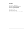
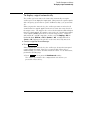
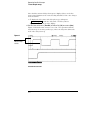
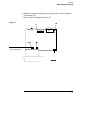
Figure 1-1 is a diagram of the front panel controls and input
connectors.
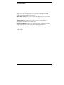
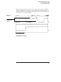
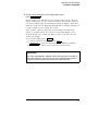
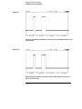
Figure 1-2 is a status line example. The status line, located at the top
of of the display, lets you quickly determine the setup of the
oscilloscope. In this chapter you will learn to read at a glance the
setup of the oscilloscope from the status line.
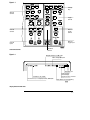
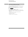
Figure 1-3 is a diagram showing which grey keys to press to bring up
the various softkey menus.
1-2
Figure 1-1
Storage
keys
General
controls
Trigger
controls
External
trigger
control
Channel
controls
External
trigger input
Channel
inputs
Horizontal
controls
Front Panel Controls
Figure 1-2
Delayed sweep is on, 500 ns/div
Main sweep 500 ms/div
Autostore is on
Channel 2 is on, 4 V/div
Channel 1 is on, ac coupled, inverted, 100 mV/div
Auto triggered,
positive slope;
trigger source is channel 1
Peak detect is on and operating
Display Status Line Indicators
1-3
Figure 1-3
Press this key
To obtain this menu
Softkey Menu Reference
1-4
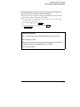
Press this key
To obtain this menu
The Oscilloscope at a Glance
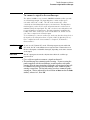
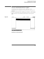
To connect a signal to the oscilloscope
To connect a signal to the oscilloscope
The Agilent 54610B is a two-channel, 500 MHz bandwidth oscilloscope with
an external trigger input. The input impedance of this oscilloscope is
selectable--either 50Ω or 1 MΩ. The 50Ω mode matches 50Ω cables
commonly used in making high frequency measurements. This impedance
matching gives you the most accurate measurements since reflections are
minimized along the signal path. The 1 MΩ mode is for use with probes and
for general purpose measurements. The higher impedance minimizes the
loading effect of the oscilloscope on the circuit under test. In this exercise
you connect a signal to the channel 1 input.
To avoid damage to your new oscilloscope, make sure that the voltage level of
the signal you are using is less than or equal to 250 V (dc plus the peak ac).
For a complete list of the characteristics see chapter 4, "Performance
Characteristics."
CAUTION
Do not exceed 5 Vrms in 50Ω mode. When input protection is enabled in
50Ω mode, the 50Ω load will disconnect if greater than 5 Vrms is detected.
However the inputs could still be damaged, depending on the time constant
of the signal.
CAUTION
The 50Ω input protection mode only functions when the oscilloscope
is powered on.
• Use a cable or a probe to connect a signal to channel 1.
• The oscilloscope has automatic probe sensing . If you are using the
probes supplied with the oscilloscope, or other probes with probe
sensing, then the input impedance and probe attenuation factors will
be automatically set up by the oscilloscope when automatic probe
sensing is turned on. The default setting is to have automatic probe
sensing on. This is indicated by the selection of Auto n under the Probe
softkey, where n is 1, 10 or 100.
1-5
The Oscilloscope at a Glance
To connect a signal to the oscilloscope
• If you are not using automatic probe sensing, then follow these next
two steps.
• To set the input impedance, press
1 . Select the desired Input
impedance of 50Ω or 1MΩ.
• To set the probe attenuation factor press 1 . Select the Next
Menu softkey. Next toggle the Probe softkey to change the
attenuation factor to match the probe you are using.
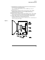
You should compensate 10:1 probes to match their characteristics to the
oscilloscope. A poorly compensated probe can introduce measurement
errors. To compensate a probe, follow these steps.
1 Connect the 10:1 probe from channel 1 to the front-panel probe adjust
signal on the oscilloscope.
2 Press Autoscale .
3 Use a nonmetallic tool to adjust the trimmer capacitor on the probe
for the flattest pulse possible as displayed on the oscilloscope.
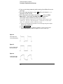
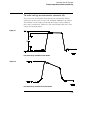
Figure 1-4
Overcompensation
causes pulse peaking.
Figure 1-5
Correct compensation
with a flat pulse top
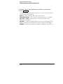
Figure 1-6
Undercompensation
causes pulse rolloff
1-6
The Oscilloscope at a Glance
To display a signal automatically
To display a signal automatically
The oscilloscope has an Autoscale feature that automatically sets up the
oscilloscope to best display the input signal. Using Autoscale requires signals
with a frequency greater than or equal to 50 Hz and a duty cycle greater than
1%.
When you press the Autoscale key, the oscilloscope turns on and scales all
channels that have signals applied, and it selects a time base range based on
the trigger source. The trigger source selected is the highest numbered input
that has a signal applied. If a signal is connected to the external trigger input
on the Agilent 54610B, then it is selected as the trigger source. Autoscale
will, in both 50Ω and 1MΩ impedance modes, reset the Coupling to DC, the
Bandwidth Limit (BW Lim) to Off, all Verniers to Off, and Signal Inversion
(Invert) to Off. Input protection in 50Ω mode is not affected by Autoscale.
1 Connect a signal to the oscilloscope.
2 Press Autoscale .
When you press the Autoscale key, the oscilloscope changes the front-panel
setup to display the signal. However, if you pressed the Autoscale key
unintentionally, you can use the Undo Autoscale feature. To use this feature,
perform the following step.
• Press
Setup
. Next, press the Undo Autoscale softkey.
The oscilloscope returns to the configuration in effect before you
pressed the Autoscale key.
1-7
The Oscilloscope at a Glance
To set up the vertical window
To set up the vertical window
The following exercise guides you through the vertical keys, knobs, and
status line.
1 Center the signal on the display with the Position knob.
The Position knob moves the signal vertically, and it is calibrated. Notice
that as you turn the Position knob, a voltage value is displayed for a short
time indicating how far the ground reference is located from the center of the
screen. Also notice that the ground symbol on the right side of the display
moves in conjunction with the Position knob.
Measurement hints
If the channel is dc coupled, you can quickly measure the dc component of the
signal by simply noting its distance from the ground symbol.
If the channel is ac coupled, the dc component of the signal is removed allowing
you to use greater sensitivity to display the ac component of the signal.
1-8
The Oscilloscope at a Glance
To set up the vertical window
2 Change the vertical setup and notice that each change affects the
status line differently.
You can quickly determine the vertical setup from the status line in the
display.
• Change the vertical sensitivity with the Volts/Div knob and notice that it
causes the status line to change.
• Press
1
.
A softkey menu appears on the display, and the channel turns on (or
remains on if it was already turned on).
• Toggle each of the softkeys and notice which keys cause the status line to
change.
Channels 1 and 2 have a vernier softkey that allows the Volt/Div knob
to change the vertical step size in smaller increments. These smaller
increments are calibrated, which results in accurate measurements
even with the vernier turned on.
• To turn the channel off, either press
1
a second time or press the
left-most softkey.
Invert operating hint
When you are triggered on the signal you are inverting, the inversion also
applies to the trigger signal (what was a rising edge now is a falling edge). If the
signal has a 50% duty cycle (square wave or sine wave), the displayed
waveform appears not to invert. However, for signals with a duty cycle other
than 50%, the displayed waveform does invert as you would expect.
1-9
The Oscilloscope at a Glance
To set up the time base
To set up the time base
The following exercise guides you through the time base keys, knobs, and
status line.
1 Turn the Time/Div knob and notice the change it makes to the status
line.
The Time/Div knob changes the sweep speed from 1 ns to 5 s in a 1-2-5 step
sequence, and the value is displayed in the status line.
2 Change the horizontal setup and notice that each change affects the
status line differently.
• Press
Main/Delayed
.
A softkey menu appears on the display with six softkey choices.
• Toggle each of the softkeys and notice which keys cause the status line to
change.
1-10
The Oscilloscope at a Glance
To set up the time base
There is also a horizontal vernier softkey that allows the Time/Div
knob to change the sweep speed in smaller increments. These smaller
increments are calibrated, which results in accurate measurements
even with the vernier turned on.
• Turn the Delay knob and notice that its value is displayed in the status line.
The Delay knob moves the main sweep horizontally, and it pauses at
0.00 s, mimicking a mechanical detent. At the top of the graticule is a
solid triangle ( ▼ ) symbol and an open triangle ( ∇ ) symbol. The ▼
symbol indicates the trigger point and it moves in conjunction with the
Delay knob. The ∇ symbol indicates the time reference point. If the
time reference softkey is set to left, the ∇ is located one graticule in
from the left side of the display. If the time reference softkey is set to
center, the ∇ is located at the center of the display. The delay number
tells you how far the reference point ∇ is located from the trigger
point ▼.
All events displayed left of the trigger point ▼ happened before the
trigger occurred, and these events are called pretrigger information or
negative time. You will find this feature very useful because you can
now see the events that led up to the trigger point. Everything to the
right of the trigger point ▼ is called posttrigger information. The
amount of delay range (pretrigger and posttrigger information)
available is dependent on the sweep speed selected. See "Horizontal
System" in chapter 4, for more details.
1-11
The Oscilloscope at a Glance
To trigger the oscilloscope
To trigger the oscilloscope
The following exercise guides you through the trigger keys, knobs, and status
line.
1 Turn the trigger Level knob and notice the changes it makes to the
display.
As you turn the Level knob or press a trigger menu key, for a short time two
things happen on the display. First, the trigger level is displayed in inverse
video. If the trigger is dc coupled, it is displayed as a voltage. If the trigger is
ac coupled or if LF reject was selected, it is displayed as a percentage of the
trigger range. Second, if the trigger source is turned on, a line is displayed
showing the location of the trigger level (as long as ac coupling or low
frequency reject are not selected).
2 Change the trigger setup and notice that each change affects the
status line differently.
• Press
Source
.
A softkey menu appears on the display showing the trigger source
choices.
• Toggle each of the softkeys and notice that each key causes the status line
to change.
3 The Agilent 54610B has a viewable external trigger, which is useful
for making timing measurements. It is also useful for ensuring that
the trigger level is not set to a value that results in trigger instability
which causes display to appear unstable. One example of this
measurement challenge is the ringing on a fast signal.
• Press
External Trigger
.
A softkey menu appears on the display showing the external trigger
choices.
Toggle each of the softkeys, turn the knob, and notice how the display
changes.
1-12
The Oscilloscope at a Glance
To trigger the oscilloscope
• Press
Mode
.
A softkey menu appears on the display with five trigger mode choices.
• Toggle the Single and TV softkeys and notice that they affect the status
line differently. (You can only select TV if the trigger source is either
channel 1 or 2.)
When the oscilloscope is triggering properly, the trigger mode portion
of the status line is blank.
What happens if the oscilloscope loses trigger?
If Auto Level is the trigger mode, Auto flashes in the status line. If dc coupled,
the oscilloscope resets the trigger level to the center of the signal. If ac
coupled, the oscilloscope resets the trigger level to halfway between the
minimum and maximum amplitudes as displayed on the screen. In addition,
every time you press the Auto Level softkey, the oscilloscope resets the trigger
level.
If Auto is the trigger mode, Auto flashes in the status line and the oscilloscope
free runs.
If either Normal or TV is the trigger mode, the trigger setup flashes in the status
line.
1-13
The Oscilloscope at a Glance
To trigger the oscilloscope
• Press
Slope/Coupling
.
A softkey menu appears on the display. If you selected Auto level,
Auto, Normal, or Single as a trigger mode, six softkey choices are
displayed. If you selected TV as a trigger source, five other softkey
choices are available.
• Toggle each of the softkeys and notice which keys affect the status line.
• On the Agilent 54610B, the external trigger input is selectable as ac or dc
coupled or ground.
3 Adjust the Holdoff knob and observe how it changes the display.
Holdoff keeps the trigger from rearming for an amount of time that you set.
Holdoff is often used to stabilize the display of complex waveforms. The
Holdoff range is from 200.0 ns to about 13.5 s. When you adjust the Holdoff
knob, the current holdoff time is briefly displayed in inverse video near the
bottom of the display. For an example of using Holdoff, refer to the section,
"To trigger on a complex waveform" on page 2-12.
To set a long holdoff time, go to a slower sweep speed.
The value used to increment the holdoff depends upon the sweep speed or
time/div selection. However, the actual holdoff value is a fixed number; it is not
a percentage of sweep speed. For a time/div setting of 5 ns/div, the holdoff
increment is about 50 ns. For a time/div setting of 5 s/div, the holdoff increment
is about 100 ms.
1-14
The Oscilloscope at a Glance
To use roll mode
To use roll mode
Roll mode continuously moves data across the display from right to left.
Roll mode allows you to see dynamic changes on low frequency signals,
such as when you adjust a potentiometer. Two frequently used applications
of roll mode are transducer monitoring and power supply testing.
1 Press Mode . Then press the Auto Lvl or Auto softkey.
2 Press Main/Delayed .
3 Press the Roll softkey.
The oscilloscope is now untriggered and runs continuously. Also notice that
the time reference softkey selection changes to center and right.
4 Press Mode . Then press the Single softkey.
The oscilloscope fills either 1/2 of the display if Center is selected for the time
reference, or 9/10 of the display if Right is selected for the time reference,
then it searches for a trigger. After a trigger is found, the remainder of the
display is filled. Then the oscilloscope stops acquiring data.
You can also make automatic measurements in the roll mode. Notice that the
oscilloscope briefly interrupts the moving data while it makes the
measurement. The acquisition system does not miss any data during the
measurement. The slight shift in the display after the measurement is
complete is that of the display catching up to the acquisition system.
Roll mode operating hints
Math functions, averaging, and peak detect are not available.
Holdoff and horizontal delay are not active.
Both a free running (nontriggered) display and a triggered display (available in
the single mode only) are available.
It is available at sweep speeds of 200 ms/div and slower.
1-15
1-16
2
Operating Your Oscilloscope
Operating Your Oscilloscope
By now you are familiar with the VERTICAL, HORIZONTAL, and TRIGGER
groups of the front-panel keys. You should also know how to
determine the setup of the oscilloscope by looking at the status line.
If you are unfamiliar with this information, we recommend you read
chapter 1, "The Oscilloscope at a Glance."
This chapter takes you through two new groups of front-panel keys:
STORAGE, and the group of keys that contains the Measure,
Save/Recall, and Display keys. You will also add to your knowledge of
the HORIZONTAL keys by using delayed sweep.
We recommend you perform all of the following exercises so you
become familiar with the powerful measurement capabilities of your
oscilloscope.
2-2
Operating Your Oscilloscope
To use delayed sweep
To use delayed sweep
Delayed sweep is a magnified portion of the main sweep. You can use
delayed sweep to locate and horizontally expand part of the main sweep for a
more detailed (high resolution) analysis of signals. The following steps show
you how to use delayed sweep. Notice that the steps are very similar to
operating the delayed sweep in analog oscilloscopes.
1 Connect a signal to the oscilloscope and obtain a stable display.
2 Press Main/Delayed .
3 Press the Delayed softkey.
The screen divides in half. The top half displays the main sweep, and the
bottom half displays an expanded portion of the main sweep. This expanded
portion of the main sweep is called the delayed sweep. The top half also has
two solid vertical lines called markers. These markers show what portion of
the main sweep is expanded in the lower half. The size and position of the
delayed sweep are controlled by the Time/Div and Delay knobs. The
Time/Div next to the
symbol is the delayed sweep sec/div. The delay
value is displayed for a short time at the bottom of the display.
• To display the delay value of the delayed time base, either
press
Main/Delayed
or turn the Delay knob.
• To change the main sweep Time/Div, you must turn off the delayed sweep.
2-3
Operating Your Oscilloscope
To use delayed sweep
Since both the main and delayed sweeps are displayed, there are half as
many vertical divisions so the vertical scaling is doubled. Notice the changes
in the status line.
• To display the delay time of the delayed sweep, either press
Main/Delayed or turn the delay knob. The delay value is
displayed near the bottom of the display.
4 Set the time reference (Time Ref) to either left (Lft) or center (Cntr).
Figure 2-1 shows the time reference set to left. The operation is like the
delayed sweep of an analog oscilloscope, where the delay time defines the
start of the delayed sweep.
Figure 2-1
Delayed sweep
markers
Time reference set to left
2-4
Operating Your Oscilloscope
To use delayed sweep
Figure 2-2 shows the time reference set to center. Notice that the markers
expand around the area of interest. You can place the markers over the area
of interest with the delay knob, then expand the delayed sweep with the time
base knob to increase the resolution.
Figure 2-2
Delayed sweep
markers
Time reference set to center
2-5
Operating Your Oscilloscope
To use storage oscilloscope operation
To use storage oscilloscope operation
There are four front-panel storage keys. They are white instant action keys
that change the operating mode of the oscilloscope. The following steps
demonstrate how to use these storage keys.
1 Connect a signal to the oscilloscope and obtain a stable display.
2 Press Autostore .
Notice that STORE replaces RUN in the status line.
For easy viewing, the stored waveform is displayed in half bright and the
most recent trace is displayed in full bright. Autostore is useful in a number
of applications.
•
•
•
•
Displaying the worst-case extremes of varying waveforms
Capturing and storing a waveform
Measuring noise and jitter
Capturing events that occur infrequently
2-6
Operating Your Oscilloscope
To use storage oscilloscope operation
3 Using the position knob in the Vertical section of the front panel,
move the trace up and down about one division.
Notice that the last acquired waveform is in full bright and the previously
acquired waveforms are displayed in half bright.
• To characterize the waveforms, use the cursors. See "To make cursor
measurements" on page 2-23.
• To clear the display, press Erase .
• To exit the Autostore mode, press either
Run
or Autostore .
Summary of storage keys
Run – The oscilloscope acquires data and displays the most recent trace.
Stop – The display is frozen.
Autostore – The oscilloscope acquires data, displaying the most recent trace in
full bright and previously acquired waveforms in half bright.
Erase – Clears the display.
2-7
Operating Your Oscilloscope
To capture a single event
To capture a single event
To capture a single event, you need some knowledge of the signal in order to
set up the trigger level and slope. For example, if the event is derived from
TTL logic, a trigger level of 2 volts should work on a rising edge. The
following steps show you how to use the oscilloscope to capture a single
event.
1 Connect a signal to the oscilloscope.
2 Set up the trigger.
• Press
• Press
Source
. Select a trigger source with the softkeys.
Slope/Coupling
. Select a trigger slope with the softkeys.
• Turn the Level knob to a point where you think the trigger should work.
3 Press Mode , then press the Single softkey.
4 Press Erase
to clear previous measurements from the display.
5 Press Run .
Pressing the Run key arms the trigger circuit. When the trigger conditions
are met, data appears on the display representing the data points that the
oscilloscope obtained with one acquisition. Pressing the Run key again
rearms the trigger circuit and erases the display.
2-8
Operating Your Oscilloscope
To capture a single event
6 If you need to compare several single-shot events,
press Autostore .
Like the Run key, the Autostore key also arms the trigger circuit. When the
trigger conditions are met, the oscilloscope triggers. Pressing the Autostore
key again rearms the trigger circuit without erasing the display. All the data
points are retained on the display in half bright with each trigger allowing you
to easily compare a series of single-shot events.
After you have acquired a single-shot event, pressing a front-panel key,
softkey, or changing a knob can erase the event from the display. If you
press the Stop key, the oscilloscope will recover the event and restore the
oscilloscope settings.
• To clear the display, press Erase .
• To exit the Autostore mode, press either
Run
or Autostore . Notice that RUN replaces STORE in the status line,
indicating that the oscilloscope has exited the Autostore mode.
Operating hint
The single-shot bandwidth is 2 MHz for single-channel operation, and 1 MHz for
two-channel operation. There are twice as many sample points per waveform
on the one-channel acquisition than on the two-channel acquisition.
2-9
Operating Your Oscilloscope
To capture glitches or narrow pulses
To capture glitches or narrow pulses
A glitch is a rapid change in the waveform that is usually narrow as compared
to the waveform. This oscilloscope has two modes of operation that you can
use for glitch capture: peak detect and Autostore.
1 Connect a signal to the oscilloscope and obtain a stable display.
2 Find the glitch.
Use peak detect for narrow pulses or glitches that require sweep speeds
slower than 50 µs/div.
• To select peak detect, press
Display
. Next, press the Peak Det
softkey.
Peak detect operates at sweep speeds from 5 s/div to 50 µs/div. When
operating, the initials Pk are displayed in the status line in inverse
video. At sweep speeds faster than 50 µs/div, the Pk initials are
displayed in normal video, which indicates that peak detect is not
operating.
2-10
Operating Your Oscilloscope
To capture glitches or narrow pulses
Use Autostore for the following cases: waveforms that are changing,
waveforms that you want to view and compare with stored waveforms,
and narrow pulses or glitches that occur infrequently but require the
use of sweep speeds outside the range of peak detect.
• Press
Autostore
.
You can use peak detect and Autostore together. Peak detect
captures the glitch, while Autostore retains the glitch on the display in
half bright video.
3 Characterize the glitch with delayed sweep.
Peak detect functions in the main sweep only, not in the delayed sweep. To
characterize the glitch with delayed sweep follow these steps.
• Press
Main/Delayed
. Next press the Delayed softkey.
• To obtain a better resolution of the glitch, expand the time base.
• To set the expanded portion of the main sweep over the glitch, use the
Delay knob.
• To characterize the glitch, use the cursors or the automatic measurement
capabilities of the oscilloscope.
2-11
Operating Your Oscilloscope
To trigger on a complex waveform
To trigger on a complex waveform
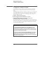
The difficulty in viewing a complex waveform is triggering on the signal.
Figure 2-3 shows a complex waveform that is not synchronized with the
trigger.
The simplest trigger method is to trigger the oscilloscope on a sync pulse that
is associated with the waveform. See "To trigger the oscilloscope" on page
1-10. If there is no sync pulse, use the following procedure to trigger on a
periodic complex waveform.
1 Connect a signal to the oscilloscope.
2 Set the trigger level to the middle of the waveform.
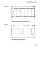
3 Adjust the Holdoff knob to synchronize the trigger of the
oscilloscope with the complex waveform.
By setting the Holdoff to synchronize the trigger, the oscilloscope ignores the
trigger that results in figure 2-3, and waits for the trigger that results in figure
2-4. Also notice in figure 2-3 that the trigger is stable, but the waveform is
not synchronized with the trigger.
Holdoff operating hints
1 The advantage of digital holdoff is that it is a fixed number. As a result,
changing the time base settings does not affect the holdoff number; so, the
oscilloscope remains triggered. In contrast, the holdoff in analog oscilloscopes
is a function of the time base setting making it necessary to readjust the holdoff
each time you change the time base setting.
2 The rate of change of the holdoff adjustment knob depends on the time base
setting you have selected. If you need a lengthy holdoff setting, increase the
time/div setting on the time base, then make your coarse holdoff adjustment.
Now switch back to the original time/div setting and make the fine adjustment to
reach the exact amount you want.
2-12
Operating Your Oscilloscope
To trigger on a complex waveform
Figure 2-3
Stable trigger, but the waveform is not synchronized with the trigger
Figure 2-4
Holdoff synchronizes the waveform with the trigger
2-13
Operating Your Oscilloscope
To make frequency measurements automatically
To make frequency measurements automatically
The automatic measurement capability of the oscilloscope makes frequency
measurements easy, as the following steps demonstrate.
1 Connect a signal to the oscilloscope and obtain a stable display.
2 Press Time .
A softkey menu appears with six softkey choices.
3 Toggle the Source softkey to select a channel for the frequency
measurement.
4 Press the Freq softkey.
The oscilloscope automatically measures the frequency and displays the
result on the lower line of the display. The number in parentheses after the
word Freq is the number of the channel that the oscilloscope used for the
measurement. The oscilloscope retains in memory and displays the three
most current measurement results. If you make a fourth measurement, the
left-most result is dropped
2-14
Operating Your Oscilloscope
To make frequency measurements automatically
If the Show Meas softkey is turned on, cursors are displayed on the
waveform that show the measurement points for the right-most
measurement result. If you select more than one measurement, you
can show a previous measurement by reselecting the measurement.
• To find the Show Meas softkey, press the Next Menu softkey.
The oscilloscope makes automatic measurements on the first
displayed event. Figure 2-5 shows how to use delayed sweep to
isolate an event for a frequency measurement. If the measurement is
not possible in the delayed time base mode, then the main time base is
used. If the waveform is clipped, it may not be possible to make the
measurement.
Figure 2-5
Delayed time base isolates an event for a frequency measurement
2-15
Operating Your Oscilloscope
To make time measurements automatically
To make time measurements automatically
You can measure the following time parameters with the oscilloscope:
frequency, period, duty cycle, width, rise time, and fall time. The following
exercise guides you through the Time keys by making a rise time
measurement. Figure 2-6 shows a pulse with some of the time measurement
points.
1 Connect a signal to the oscilloscope and obtain a stable display.
When the signal has a well-defined top and bottom, the rise time and fall time
measurements are made at the 10% and 90% levels. If the oscilloscope
cannot find a well-defined top or bottom, the maximum and minimum levels
are used to calculate the 10% and 90% points. These levels are shown on
page 2-19 in figures 2-8 and 2-9.
Figure 2-6
2-16
Operating Your Oscilloscope
To make time measurements automatically
2 Press Time .
A softkey menu appears with six softkey choices. Three of the softkeys are
time measurement functions.
Source Selects a channel for the time measurement.
Time Measurements Three time measurement choices are available: Freq
(frequency), Period, and Duty Cy (duty cycle). These measurements are
made at the 50% levels. Refer to figure 2-6.
Clear Meas (clear measurement) Erases the measurement results and
removes the cursors from the display.
Next Menu Replaces the softkey menu with six additional softkey choices.
3 Press the Next Menu softkey.
Another time measurement softkey menu appears with six additional choices.
Four of the softkeys are time measurement functions.
Show Meas (show measurement) Displays the horizontal and vertical cursors
where the measurement was taken.
2-17
Operating Your Oscilloscope
To make time measurements automatically
Time Measurements Four additional time measurement choices are available;
+Width, [Pulse Width] -Width, Rise Time, and Fall Time. Width measurements
are made at the 50% levels, whereas rise time and fall time measurements are
made at the 10% to 90% levels.
Previous Menu Returns to the previous softkey menu.
4 Press the Rise Time softkey.
The oscilloscope automatically measures the rise time of the signal and
displays the result on the display.
The oscilloscope makes automatic measurements on the first displayed
event. Figure 2-7 shows how to use delayed sweep to isolate an edge for a
rise time measurement.
Figure 2-7
Delayed sweep isolates a leading edge for a rise time measurement
2-18
Operating Your Oscilloscope
To make voltage measurements automatically
To make voltage measurements automatically
You can measure the following voltage parameters automatically with the
oscilloscope: peak-to-peak, average, rms, maximum, minimum, top, and base.
The following exercise guides you through the Voltage keys by making an
rms voltage measurement. Figures 2-8 and 2-9 show pulses with some of the
voltage measurement points.
Figure 2-8
Pulse where the top and bottom are well-defined
Figure 2-9
Pulse where the top and bottom are not well-defined
2-19
Operating Your Oscilloscope
To make voltage measurements automatically
1 Connect a signal to the oscilloscope and obtain a stable display.
2 Press Voltage .
A softkey menu appears with six softkey choices. Three of the softkeys are
voltage measurement functions.
Source Selects a channel for the voltage measurement.
Voltage Measurements Three voltage measurement choices are available:
Vp-p, Vavg, and Vrms. The measurements are determined by voltage
histograms of the signal.
Clear Meas (clear measurement) Erases any measurement results from the
display, and removes the horizontal and vertical cursors from the display.
Next Menu Replaces the softkey menu with six additional softkey choices.
2-20
Operating Your Oscilloscope
To make voltage measurements automatically
3 Press the Vrms softkey.
The oscilloscope automatically measures the rms voltage and displays the
result on the display.
The oscilloscope makes automatic measurements on the first pulse or period
in the display. Figure 2-10 shows how to use delayed sweep to isolate a pulse
for an rms measurement.
Figure 2-10
Delayed sweep isolates an area of interest for an rms voltage measurement
2-21
Operating Your Oscilloscope
To make voltage measurements automatically
4 Press the Next Menu softkey.
Another voltage measurement softkey menu appears with six additional
choices. Four of the softkeys are voltage measurement functions.
Show Meas (show measurement) Displays the horizontal and vertical cursors
that show where the measurement was taken on the signal.
Voltage Measurements Four additional voltage measurement choices are
available: Vmax, Vmin, Vtop, Vbase.
Previous Menu Returns to the previous softkey menu.
2-22
Operating Your Oscilloscope
To make cursor measurements
To make cursor measurements
The following steps guide you through the front-panel Cursors key. You can
use the cursors to make custom voltage or time measurements on the signal.
Examples of custom measurements include rise time measurements from
reference levels other than 10-90%, frequency and width measurements from
levels other than 50%, channel-to-channel delay measurements, and voltage
measurements. See figures 2-11 through 2-16 for examples of custom
measurements.
1 Connect a signal to the oscilloscope and obtain a stable display.
2 Press Cursors .
A softkey menu appears with six softkey choices. Four of the softkeys are
cursor functions.
Source Selects a channel for the voltage cursor measurements.
Active Cursor There are four cursor choices: V1, and V2 are voltage
cursors, while t1, and t2 are time cursors. Use the knob below the
Cursors key to move the cursors. When you press the V1 and V2
softkeys simultaneously or the t1 and t2 softkeys simultaneously, the
cursors move together.
Clear Cursors Erases the cursor readings and removes the cursors from the
display.
2-23
Operating Your Oscilloscope
To make cursor measurements
Figure 2-11
Cursors used to measure pulse width at levels other then the 50% points
Figure 2-12
Cursors used to measure the frequency of the ringing on a pulse
2-24
Operating Your Oscilloscope
To make cursor measurements
Figure 2-13
Cursors used to make channel-to-channel delay measurements
Figure 2-14
The cursors track delayed sweep. Expand the display with delayed sweep, then characterize
the event of interest with the cursors.
2-25
Operating Your Oscilloscope
To make cursor measurements
Figure 2-15
Pressing t1 and t2 softkeys simultaneously causes the cursors to move together when the cursor
knob is adjusted.
Figure 2-16
By moving the cursors together, you can check for pulse width variations in a pulse train, as
figures 2-15 and 2-16 show.
2-26
Operating Your Oscilloscope
To remove cabling errors from time interval measurements
To remove cabling errors from time interval
measurements
When measuring time intervals in the nanosecond range, small differences in
cable length can totally obscure the measurement. The following exercise
shows how to remove errors that different cable lengths or characteristics
introduce to your measurement. The Skew control makes it possible to
remove this offset error from your measurement.
This process is also referred to as deskewing.
1 Select Time Reference to Center, with the Graticule turned on.
2 Connect the channels to be nulled to a common test point and obtain
a stable display. A fast edge is a good choice.
3 Press Print/Utility , then select the Self Cal menu. This gives
you access to the calibration and skew adjustments.
4 Select Skew 1 > 2 to adjust channel 2 with respect to channel 1. Rotate
the knob to bring the channels into time alignment. This nullifies the
cable delay.
5 Select Skew 1 > E to adjust the External Trigger with respect to
Channel 1. Rotate the knob to bring these channels into time
alignment..
Note: This adjustment is not affected by pressing Autoscale. Only the
default setup will return the skew values to zero seconds.
2-27
Operating Your Oscilloscope
To make setup and hold time measurements
To make setup and hold time measurements
One method of testing a device for its setup and hold times limits uses a
variable pulse generator to provide the time varying pulses, and an
oscilloscope to monitor when the setup and hold times are violated.
Selecting the trigger for this measurement is important. The clock is not a
good choice for a trigger because it is not unique. Triggering on the Q output
results in loss of trigger when the setup and hold time is violated. Triggering
on the D input is the best choice. In this example the flip flop is clocked on
the rising edge.
1 Set time skew to remove errors introduced by different cables for
2
3
4
5
6
this time interval measurement.
Connect the D input of the flip-flop to the External Trigger on your
oscilloscope. Set the scope to trigger on the rising edge.
Connect the flip-flop’s clock signal to channel 1.
Connect the Q output to channel 2 of the oscilloscope.
Press Autoscale , then turn on the External Trigger so that it is
viewable.
Use the time cursors to measure the difference between the rising
edge of the clock and the D input to determine setup and hold time.
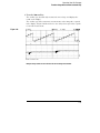
Figure 2-17
Setup time measurement: channel 1 = clock, channel 2 = Q output, and
External Trigger = D input
2-28
Operating Your Oscilloscope
To view asynchronous noise on a signal
To view asynchronous noise on a signal
The following exercise shows how to use the oscilloscope to view
asynchronous noise on a signal that is not synchronous to the period of the
waveform.
1 Connect a noisy signal to the oscilloscope and obtain a stable display.
Figure 2-18 shows a waveform with asynchronous noise at the top of the
pulse.
Figure 2-18
Asynchronous noise at the top of the pulse
2-29
Operating Your Oscilloscope
To view asynchronous noise on a signal
2 Press Autostore .
Notice that STORE is displayed in the status line.
3 Set the Trigger Mode to Normal, then adjust the trigger level into the noise
region of the signal.
4 Decrease the sweep speed for better resolution of the asynchronous
noise.
• To characterize the asynchronous noise signal, use the cursors.
Figure 2-19
This is a triggered view of the asynchronous noise shown in figure 2-18.
2-30
Operating Your Oscilloscope
To reduce the random noise on a signal
To reduce the random noise on a signal
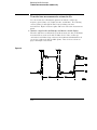
If the signal you are applying to the oscilloscope is noisy (figure 2-22), you
can set up the oscilloscope to reduce the noise on the waveform (figure
2-23). First, you stabilize the displayed waveform by removing the noise
from the trigger path. Second, you reduce the noise on the displayed
waveform.
1 Connect a signal to the oscilloscope and obtain a stable display.
2 Remove the noise from the trigger path by turning on either high
frequency reject or noise reject.
High frequency reject (HF Reject) adds a low pass filter with the 3 dB point at
50 kHz (see figure 2-20). You use HF reject to remove high frequency noise
such as AM or FM broadcast stations from the trigger path.
Figure 2-20
0 dB
3 dB down point
Pass
Band
dc
50 kHz
HF reject
2-31
Operating Your Oscilloscope
To reduce the random noise on a signal
Low frequency reject (LF Reject) adds a high pass filter with the 3-dB point at
50 kHz (see figure 2-21). Use LF reject to remove low frequency signals such
as power line noise from the trigger path.
Figure 2-21
0 dB
3 dB down point
Pass
Band
dc
50 kHz
LF reject
Noise reject increases the trigger hysteresis band. By increasing the trigger
hysteresis band you reduce the possibility of triggering on noise. However,
this also decreases the trigger sensitivity so that a slightly larger signal is
required to trigger the oscilloscope.
Figure 2-22
Random noise on the displayed waveform
2-32
Operating Your Oscilloscope
To reduce the random noise on a signal
3 Use averaging to reduce noise on the displayed waveform.
To use averaging follow these steps.
• Press
Display
, the press the Average softkey.
Notice that Av appears in the status line.
• Toggle the # Average softkey to select the number of averages that best
eliminates the noise from the displayed waveform.
The Av letters in the status line indicate how much of the averaging
process is finished by turning to inverse video as the oscilloscope
performs averaging. The higher the number of averages, the more
noise that is removed from the display. However, the higher the
number of averages, the slower the displayed waveform responds to
waveform changes. You need to choose between how quickly the
waveform responds to changes and how much noise there is on the
signal.
Figure 2-23
On this waveform, 256 averages were used to reduce the noise
2-33
Operating Your Oscilloscope
To analyze video waveforms
To analyze video waveforms
The TV sync separator in the oscilloscope has an internal clamp circuit. This
removes the need for external clamping when you are viewing unclamped
video signals. TV triggering requires two vertical divisions of display, either
channel 1 or channel 2 as the trigger source, and the selection of internal
trigger. Turning the trigger level knob in TV trigger does not change the
trigger level because the trigger level is automatically set to the sync pulse
tips.
For this exercise connect the oscilloscope to the video output terminals on a
television. Then set up the oscilloscope to trigger on the start of Frame 2.
Use the delayed sweep to window in on the vertical interval test signals
(VITS), which are in Line 18 for most video standards (NTSC, PAL, SECAM).
1 Connect a TV signal to channel 1, then press Autoscale .
2 Press Display , then press the Peak Det softkey.
3 Press Mode , then press the TV softkey.
4 Press Slope/Coupling , then press the Field 2 softkey.
2-34
Operating Your Oscilloscope
To analyze video waveforms
Polarity
Selects either positive or negative sync pulses.
Field 1
Field 2
Triggers on the field 1 portion of the video signal.
Triggers on the field 2 portion of the video signal.
Line Triggers on all the TV line sync pulses.
HF Rej Controls a 500 kHz low pass filter in the trigger path.
5 Set the time base to 200 µs/div, then center the signal on the display
with the delay knob (delay about 800 µs).
6 Press Main/Delayed , then press the Delayed softkey.
7 Set the delayed sweep to 20 µs/div, then set the expanded portion
over the VITS (delay about 988.8 µs).
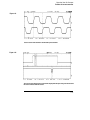
Figure 2-24
Frame 2 windowed on the VITS in Line 18
2-35
Operating Your Oscilloscope
To analyze video waveforms
8 Press Main/Delayed , then press the Main softkey.
9 Use the horizontal vernier to change the time base to 7 µs/div, then
center the signal on the display with the delay knob (delay about
989 µs).
Figure 2-25
Full screen display of the IRE
2-36
Operating Your Oscilloscope
To analyze video waveforms
Delay in TV line units hint
The Agilent 54610B oscilloscope has the ability to display delay in TV-line units.
Using the TV field trigger mode activates this line-counting feature. When Field
1 or Field 2 is selected as the trigger source, delay can be set in terms of time or
line number.
Both-fields triggering in the Agilent 54610B hint
The Agilent 54610B can trigger on the vertical sync pulse in both TV fields at the
same time. This allows you to view noninterlaced video signals which are
common in computer monitors. To trigger on both sync pulses, press Field 1 and
Field 2 at the same time.
TV trigger operating hints
The color burst changes phase between odd (Fields 1 and 3) and even (Fields 2
and 4). It looks double-triggered. Increase the holdoff to greater than the frame
width to finetune your trigger stability. For example, use a holdoff value of
around 63 ms for NTSC, and around 76 ms for PAL.
When looking at live video (usually a field), use peak detect to improve the
appearance of the display.
When making cursor measurements, use Autostore since you are usually
looking for pulse flatness and extremes.
When using line trigger, use minimum holdoff to display all the lines. Due to the
relationship between the horizontal and vertical sync frequencies the display
looks like it is untriggered, but it is very useful for TV waveform analysis and
adjustment because all of the lines are displayed.
2-37
Operating Your Oscilloscope
To save or recall traces
To save or recall traces
The oscilloscope has two pixel memories for storing waveforms. The
following exercise guides you through how to store and recall waveforms
from pixel memories.
1 Connect a signal to the oscilloscope and obtain a stable display.
2 Press
Trace
.
A softkey menu appears with five softkey selections. Four of the softkeys are
trace memory functions.
Trace Selects memory 1 or memory 2.
Trace Mem Turns on or off the selected memory.
Save to Saves the waveform to the selected memory. The front-panel setup
is saved to a separate memory location.
Clear Erases the selected memory.
Recall Setup Recalls the front-panel setup that was saved with the
waveform.
3 Toggle the Trace softkey to select memory 1 or memory 2.
4 Press the Save to softkey.
The current display is copied to the selected memory.
5 Turn on the Trace Mem softkey to view the stored waveform.
The trace is copied from the selected trace memory and is displayed in half
bright video.
2-38
Operating Your Oscilloscope
To save or recall front-panel setups
The automatic measurement functions do not operate on stored traces.
Remember, the stored waveforms are pictorial information rather than stored
data.
• If you have not changed the oscilloscope setup, use the cursors to make
the measurements.
• If you have changed the oscilloscope setup, press the Recall Setup softkey.
Then,use the cursors to make the measurements.
Trace memory operating hint
The standard oscilloscope has volatile trace memories. When you add an
interface module to the oscilloscope, the trace memories become nonvolatile.
To save or recall front-panel setups
There are 16 memories for storing front-panel setups. Saving front-panel
setups can save you time in situations where several setups are repeated
many times.
1 Press Setup .
2 To change the selected memory location, press either the left-most
softkey or turn the knob closest to the Cursors key.
3 Press the Save softkey to save a front-panel setup, then press the Recall
softkey to recall a front-panel setup.
2-39
Operating Your Oscilloscope
To use the XY display mode
To use the XY display mode
The XY display mode converts the oscilloscope from a volts versus time
display to a volts versus volts display. You can use various transducers so the
display could show strain versus displacement, flow versus pressure, volts
versus current, or voltage versus frequency. This exercise shows a common
use of the XY display mode by measuring the phase shift between two signals
of the same frequency with the Lissajous method.
1 Connect a signal to channel 1, and a signal of the same frequency but
out of phase to channel 2.
2 Press Autoscale , press Main/Delayed , then press the XY
softkey.
3 Center the signal on the display with the Position knobs, and use the
Volts/Div knobs and the vertical Vernier softkeys to expand the signal
for convenient viewing.
sin θ =
Figure 2-26
2-40
A
C
or
B
D
Operating Your Oscilloscope
To use the XY display mode
Figure 2-27
4 Press Cursors .
5 Set the Y2 cursor to the top of the signal, and set Y1 to the bottom of
the signal.
Note the ∆Y value at the bottom of the display. In this example we are using
the Y cursors, but you could have used the X cursors instead. If you use the
X cursors, make sure you center the signal in the Y axis.
Figure 2-28
2-41
Operating Your Oscilloscope
To use the XY display mode
6 Move the Y1 and Y2 cursors to the center of the signal.
Again, note the ∆Y value.
Figure 2-29
7 Calculate the phase difference using formula below.
sin θ =
2-42
second ∆Y 111.9
=
= 27.25 degrees of phase shift.
244.4
first ∆Y
Operating Your Oscilloscope
To use the XY display mode
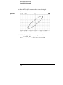
Figure 2-30
Signals are 90° out of phase
Figure 2-31
Signals are in phase
2-43
Operating Your Oscilloscope
To use the XY display mode
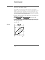
XY display mode operating hint
When you select the XY display mode, the time base is turned off. Channel 1 is
the X-axis input, channel 2 is the Y-axis input, and the external trigger in the
Agilent 54610B is the Z-axis input. If you only want to see portions of the Y
versus X display, use the Z-axis input. Z-axis turns on and off the trace (analog
oscilloscopes called this Z-blanking because it turned the beam on and off).
When Z is low (<1.3 V), Y versus X is displayed; when Z is high (>1.3 V), the trace
is turned off.
2-44
3
Verifying Oscilloscope Performance 3–5
Adjusting the Oscilloscope 3–21
Troubleshooting the Oscilloscope 3–30
Replacing Parts in the Oscilloscope 3–39
Service
Service
If the oscilloscope is under warranty, you must return it to Agilent
Techologies for all service work covered by the warranty. See "To
return the oscilloscope to Agilent Techologies," on page 3-4. If the
warranty period has expired, you can still return the oscilloscope to
Agilent Techologies for all service work. Contact your nearest Agilent
Techologies Sales Office for additional details on service work.
If the warranty period has expired and you decide to service the
oscilloscope yourself, the instructions in this chapter can help you
keep the oscilloscope operating at optimum performance.
This chapter is divided into the following four sections:
•
•
•
•
Verifying Oscilloscope Performance on page 3-5
Adjusting the Oscilloscope on page 3-21
Troubleshooting the Oscilloscope on page 3-30
Replacing Parts in the Oscilloscope on page 3-39. Service should be
performed by trained service personnel only. Some knowledge of
the operating controls is helpful, and you may find it helpful to read
chapter 1, "The Oscilloscope at a Glance."
3-2
Service
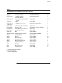
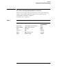
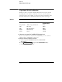
Table 3-1
Recommended list of test equipment to service the oscilloscope
Equipment
Critical specifications
Recommended Model/Part
Use1
Signal generator
1 to 500 MHz at 200 mV
high stability timebase
Agilent 8656B Option 001
P
Digital multimeter
0.1 mV resolution, better than 0.01%
accuracy
Agilent 34401A
P, A, T
Oscilloscope
100 MHz
Agilent 54600A
T
Power meter and
Power sensor
1 to 500 MHz ±3% accuracy
Agilent 436A and Agilent 8482A
P
Power supply
14 mV to 35 Vdc, 0.1 mV resolution
Agilent 6114A
P
Pulse generator
Rise time < 175 ps
PSPL 1107B TD and PSPL 1110B Driver
A
Pulse generator
10 kHz, 500 mV p-p, rise time <5 ns
Agilent 8112A
A
Power splitter
Outputs differ < 0.15 dB
Agilent 11667B
P
Shorting cap
BNC
Agilent 1250-0774
P
Time Mark Generator Stability 5 ppm after 30 minutes
Tektronix TG501A and TM503B
P
Adapter
SMA (f) to BNC (m)
Agilent 1250-1787
A
Adapter
BNC (f-f)
Agilent 1250-0080
P, A
Adapter
BNC tee (m) (f) (f)
Agilent 1250-0781
P, A
Adapter
N (m) to BNC (f), Qty 3
Agilent 1250-0780
P
Adapter
BNC (f) to dual banana (m)
Agilent 1251-2277
P
Adapter
Type N (m) to BNC (m)
Agilent 1251-0082
P
Cable
BNC, Qty 3
Agilent 10503A
P, A
Cable
BNC, 9 inches, Qty 2
Agilent 10502A
P, A
Cable
Type N (m) 24 inch
Agilent 11500B
P
P = Use for Performance Verification.
A = Use for Adjustments.
T = Use for Troubleshooting.
3-3
Service
To return the oscilloscope to Agilent Techologies
To return the oscilloscope to Agilent Techologies
Before shipping the oscilloscope to Agilent Techologies, contact your nearest
Agilent Techologies Sales Office for additional details.
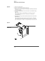
1 Write the following information on a tag and attach it to the
oscilloscope.
•
•
•
•
Name and address of owner
Model number
Serial number
Description of service required or failure indications
2 Remove all accessories from the oscilloscope.
The accessories include the power cord, probes, cables, and any modules
attached to the rear of the oscilloscope. Do not ship accessories back to
Agilent Techologies unless they are associated with the failure symptoms.
3 Protect the control panel with cardboard.
4 Pack the oscilloscope in styrofoam or other shock-absorbing material
and place it in a strong shipping container.
You can use either the original shipping containers, or order materials from
an Agilent Sales Office. Otherwise, pack the oscilloscope in 3 to 4 inches of
shock-absorbing material to prevent movement inside the shipping container.
5 Seal the shipping container securely.
6 Mark the shipping container as FRAGILE.
3-4
Verifying Oscilloscope Performance
This section shows you how to verify the electrical performance of the
oscilloscope, using the performance characteristics in chapter 4 as the
standard. The characteristics checked are dc calibrator, voltage
measurement accuracy, bandwidth, horizontal accuracy, and trigger
sensitivity.
You should verify the performance of the oscilloscope when you first
receive it, and every 12 months or after 2,000 hours of operation.
Also, make sure you allow the oscilloscope to operate for at least 30
minutes before you begin the following procedures.
Perform self-calibration first
For the oscilloscope to meet all of the verifications tests in the ambient
temperature where it will be used, the self-calibration tests described on
page 3-24 should first be performed. Allow the unit to operate for at least
30 minutes before performing the self-calibration.
Each procedure lists the recommended equipment for the test. You
can use any equipment that meets the critical specifications.
However, the procedures are based on the recommended model or
part number.
On page 3-20 of this chapter is a test record for recording the test
results of each procedure. Use the test results to gauge the
performance of the oscilloscope over time.
3-5
Service
Verifying Oscilloscope Performance
To check the output of the DC CALIBRATOR
In this test you measure the output of the DC CALIBRATOR with a multimeter.
The DC CALIBRATOR is used for self-calibration of the oscilloscope. The
accuracy is not specified, but it must be within the test limits to provide for
accurate self-calibration.
Test limits: 5.000 V ±10 mV and 0.000 V ± 500 µV.
Table 3-2
Equipment Required
Equipment
Critical specifications
Recommended
Agilent Model/Part
Digital Multimeter
0.1% mV revolution, better than 0.01%
accuracy
34401A
Cable
BNC
10503A
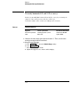
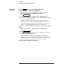
1 Connect a multimeter to the rear panel DC CALIBRATOR connector.
2 Press Print/Utility .
3 Press the Self Test softkey, then press the DAC softkey.
The multimeter should measure 0.00 V dc ± 500 µV. If the result is not
within the test limits, see "Troubleshooting the oscilloscope," on page 3-30.
4 Press any key to continue the test.
The multimeter should read 5.000 V ±10 mV. If the result is not within the
test limits, see "Troubleshooting the oscilloscope," on page 3-30.
3-6
Service
Verifying Oscilloscope Performance
To verify voltage measurement accuracy
In this test you verify the voltage measurement accuracy by measuring the
output of a power supply using dual cursors on the oscilloscope, and
comparing the results with a multimeter.
Test limits: ±2.4% of full scale.
Table 3-3
Equipment Required
Equipment
Critical specifications
Recommended
Agilent Model/Part
Power supply
14 mV to 35 Vdc, 0.1 mV resolution
6114A
Digital multimeter
Better than 0.1% accuracy
34401A
Cable
BNC, Qty 2
10503A
Shorting cap
BNC
1250-0774
Adapter
BNC (f) to banana (m)
1251-2277
Adapter
BNC tee (m) (f) (f)
1250-0781
3-7
Service
Verifying Oscilloscope Performance
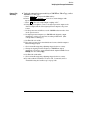
1 Set up the oscilloscope.
a Press Setup , then press the Default Setup softkey.
b Press Voltage , then press the Vavg softkey.
c Set the Volts/Div to the first line of table 3-4.
d Adjust the channel 1 Position knob to place the baseline near
(but not at) the bottom of the display.
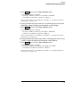
2 Press
Cursors
, then press the V1 softkey.
3 Using the cursors knob, set the V1 cursor on the baseline.
If you are in an electrically noisy environment, it can help to place a shorting
cap on the input BNC connector when positioning V1.
4 Connect the power supply to the oscilloscope and to the multimeter,
using the BNC tee and cables.
5 Set the power supply output to the first line in table 3-4.
3-8
Service
Verifying Oscilloscope Performance
6 Press the V2 softkey, then position the V2 cursor to the baseline.
The ∆V value at the bottom of the display should be within the test limits of
table 3-4. If a result is not within the test limits, see "Troubleshooting the
Oscilloscope," on page 30.
7 Continue checking the voltage measurement accuracy with the
remaining lines in table 3-4.
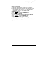
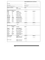
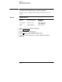
Table 3-4
Voltage Measurement Accuracy
Volts/Div setting
Power supply setting
Test limits
5 V/Div
35 V
34.04 V
to
35.96 V
2 V/Div
14 V
13.616 V
to
14.384 V
1 V/Div
7V
6.808 V
to
7.192 V
0.5 V/Div
3.5 V
3.404 V
to
3.596 V
0.2 V/Div
1.4 V
1.3616 V
to
1.4384 V
0.1 V/Div
700 mV
680.8 mV
to
719.2 mV
50 mV/Div
350 mV
340.4 mV
to
359.6 mV
20 mV/Div
140 mV
136.16 mV
to
143.84 mV
10 mV/Div
70 mV
68.08 mV
to
71.92 mV
5 mV/Div*
35 mV
33.66 mV
to
36.34 mV
2 mV/Div*
14 mV
12.66 mV
to
15.34 mV
*Full scale is defined as 56 mV on the 5 mV/div and 2 mV/div ranges.. Full scale on all
other ranges is defined as 8 divisions.
8 Disconnect the power supply from the oscilloscope, then repeat
steps 1 to 7 for channel 2.
3-9
Service
Verifying Oscilloscope Performance
To verify bandwidth
In this test you verify bandwidth by using a power meter and power sensor to
set output of a signal generator at 1 MHz and the upper bandwidth limit. You
use the peak-to-peak voltage at 1 MHz and the upper bandwidth limit to
calculate the bandwidth response of the oscilloscope.
Test limits:
Agilent 54610B, all channels (−3 dB)
dc to 500 MHz
ac coupled 10 Hz to 500 MHz.
Table 3-5
Equipment Required
Equipment
Critical specifications
Recommended
Agilent Model/Part
Signal generator
1 to 500 MHz at 200 mV
8656B opt 001
Power meter and
Power Sensor
1 to 500 MHz ±3% accuracy
436A and 8482A
Power splitter
Outputs differ by < 0.15 dB
11667B
Cable
Type N (m), 24 inch
11500B
Adapter
Type N (m) to BNC (m)
1251-0082
3-10
Service
Verifying Oscilloscope Performance
1 Connect the equipment.
a Connect the signal generator to the input of the power splitter.
b Connect the power sensor to one output of the power splitter, and
connect channel 1 of the oscilloscope to the other power splitter
output. Set the oscilloscope input impedance to 50Ω.
2 Set up the oscilloscope.
a Press Setup , then press the Default Setup softkey.
b Set the time base to 500 ns/div.
c Press 1 to select channel 1, then select 50Ω input and 100 mV/div.
d Press Display , then press the Average softkey.
e Toggle the # Average softkey to select 8 averages.
3 Set the signal generator for 1 MHz at about 5.6 dBm.
Notice that the signal on the display is about 5 cycles and six divisions of
amplitude.
3-11
Service
Verifying Oscilloscope Performance
4 Press Voltage , then press the Vp-p softkey.
Wait a few seconds for the measurement to settle (averaging is complete),
then note the Vp-p reading from the bottom of the display.
Vp-p = _______ mV.
5 Set the calibration factor percent of the power meter to the 1 MHz
value from the calibration chart on the probe, then press dB (REF)
on the power meter to set a 0 dB reference.
6 Change the frequency of the signal generator to 500 MHz
7 Set the calibration factor of the power meter to 500 MHz percent
value from the chart on the probe.
Adjust the amplitude of the signal generator for a power reading as close as
possible to 0.0 dB (REL). Power meter reading = ______ dB.
3-12
Service
Verifying Oscilloscope Performance
8 Change the time base to 5 ns/div.
Wait a few seconds for the measurement to settle (averaging is complete),
then note the Vp-p reading from the bottom of the display.
Vp-p = ______ mV.
9 Calculate the response using the following formula.
 step 8 result 
20 log10 

 step 4 result
10 Correct the result from step 9 with any difference in the power meter
reading from step 7. Make sure you observe all number signs.
For example:
Result from step 9 = −2.3 dB
Power meter reading from step 7 = −0.2 dB (REL)
True response = (−2.3) − (−0.2) = −2.1 dB
The true response should be ≤−3 dB.
If the result is not ≤−3 dB, see "Troubleshooting the Oscilloscope," on page
3-30.
11 Repeat steps 1 to 10 for channel 2.
3-13
Service
Verifying Oscilloscope Performance
To verify horizontal ∆t and 1/∆t accuracy
In this test you verify the horizontal ∆t and 1/∆t accuracy by measuring the
output of a time mark generator with the oscilloscope.
Test limits: ±0.01% ±0.2% of full scale ±200 ps (same channel)
Table 3-6
Equipment Required
Equipment
Critical specifications
Recommended Model/Part
Time marker generator
Stability 5 ppm after 1/2 hour
TG 501A and TM 503B
Cable
BNC, 3 feet
Agilent 10503A
1 Connect the time mark generator to channel 1. Then, set the time
mark generator for 0.1 ms markers.
2 Setup the oscilloscope.
a Press Setup , then press the Default Setup softkey.
b Press Autoscale .
c Set the time base to 20 µs/div.
d Adjust the trigger level to obtain a stable display.
3-14
Service
Verifying Oscilloscope Performance
3 Press Time , then press the Freq and Period softkeys.
You should measure the following:
Frequency 10 kHz, test limits are 9.959 kHz to 10.04 kHz.
Period 100 µs, test limits are 99.59 µs to 100.4 µs.
If the measurements are not within the test limits, see "Troubleshooting the
Oscilloscope," on page 3-30.
4 Change the time mark generator to 1 µs, and change the time base to
200 ns/div. Adjust the trigger level to obtain a stable display.
5 Press Time , then press the Freq and Period softkeys.
You should measure the following:
Frequency 1 MHz, test limits are 995.7 kHz to 1.004 MHz.
Period 1 µs, test limits are 995.7 ns to 1.004 µs.
If the measurements are not within the test limits, see "Troubleshooting the
Oscilloscope," on page 3-30.
6 Change the time mark generator to 20 ns, and change the time base to
5 ns/div. Adjust the trigger level to obtain a stable display.
7 Press Time , then press the Freq and Period softkeys.
You should measure the following:
Frequency 50 MHz, test limits are 49.25 MHz to 50.77 MHz.
Period 20 ns, test limits are 19.70 ns to 20.30 ns.
If the measurements are not within the test limits, see "Troubleshooting the
Oscilloscope," on page 3-30.
3-15
Service
Verifying Oscilloscope Performance
8 Change the time mark generator to 2 ns, and change the time base to
1 ns/div. Adjust the trigger level to obtain a stable display.
9 Press Time , then press the Freq and Period softkeys.
You should measure the following:
Frequency 500 MHz, test limits are 446.4 MHz to 568.2 MHz.
Period 2 ns, test limits are 1.760 ns to 2.240 ns.
If the measurements are not within the test limits, see "Troubleshooting the
Oscilloscope," on page 3-30.
3-16
Service
Verifying Oscilloscope Performance
To verify trigger sensitivity
In this test you verify the trigger sensitivity by applying 100 MHz to the
oscilloscope. The amplitude of the signal is decreased to the specified levels,
then you check to see if the oscilloscope is still triggered. You then repeat
the process at the upper bandwidth limit.
Test limits:
Internal trigger
dc to 100 MHz, 0.5 div or 5.0 mV p-p
100 MHz to 500 MHz, 1 div or 10 mV p-p
External trigger
dc to 100 MHz, <75 mV p-p
100 MHz to 500 MHz, <150 mV p-p
Table 3-7
Equipment Required
Equipment
Critical specifications
Recommended
Agilent Model/Part
Signal generator
100 MHz and 500 MHz sine waves
8656B Option 001
Power splitter
Outputs differ < 0.15 dB
11667B
Cable
BNC, Qty 3
10503A
Adapter
N (m) to BNC (f), Qty 3
1250-0780
Power meter and
Power sensor
1 to 500 MHz +/-3%
436A and 8482A
3-17
Service
Verifying Oscilloscope Performance
Internal Trig
Sensitivity
1 Press Setup , then press the Default Setup softkey.
2 Connect the signal generator to channel 1.
3 Verify the trigger sensitivity at 100 MHz and 0.5 divisions.
a Set the signal generator to 100 MHz and about 50 mV.
b Press Autoscale .
c Press 1 to select channel 1, then select 50Ω input impedance.
d Decrease the output of the signal generator until there is 0.35 vertical
divisions of the signal displayed.
The trigger should be stable. If the triggering is not stable, try
adjusting the trigger level. If adjusting the trigger level makes the
triggering stable, the test still passes. If adjusting the trigger does not
help, see "Troubleshooting the Oscilloscope," on page 3-30.
4 Verify the trigger sensitivity at 1 division for the frequency shown
below.
a Change the output of the signal generator to 500 MHz and set
amplitude to about 100 mV.
b Press Autoscale .
c Decrease the output of the signal generator until there is 1 vertical
division of the signal displayed.
The trigger should be stable. If the triggering is not stable, try
adjusting the trigger level. If adjusting the trigger level makes the
triggering stable, the test still passes. If adjusting the trigger does not
help, see "Troubleshooting the Oscilloscope," on page 3-30.
5 Repeat steps 1 through 4 for channel 2.
3-18
Service
Verifying Oscilloscope Performance
External Trig
Sensitivity
6 Verify the external trigger sensitivity at 500 MHz at 150 mV p-p, and at
100 MHz at 75 mV p-p.
a Press
c Press
b
Source , then press the Ext softkey.
External Trigger
, then select external trigger with
input coupling of 50Ω.
1
then select signal input coupling of 50 Ω.
Using the power splitter, connect one signal generator output to the
channel 1 input and the other signal generator output to the power
sensor.
Set the power meter Cal Factor to the 500 MHz value from the chart
on the power sensor.
Set signal generator frequency to 500 MHz and adjust the output
amplitude to achieve a power meter reading of 0.075 mW. (This
corresponds to 150 mV p-p.)
Set Time/div to 1 ns/div.
Disconnect power meter from divider and connect divider output to
External Trigger Input.
Check for stable triggering, adjusting trigger level if necessary.
Change the signal generator frequency to 100 MHz at output
amplitude of 75 mV p-p, as measured with the Agilent 54610B. Press
Voltage, then the softkey Vp-p.
Set Time/div to 10 ns/div.
Check for stable triggering, adjusting trigger level if necessary.
Record results in Performance Test Record. If test fails, refer to
"Troubleshooting the Oscilloscope" on page 3-30.
c Press
d
e
f
g
h
i
j
k
l
m
3-19
Agilent 54610B Performance Test Record
Serial No. ______________________________________
Test by_____________________________________
Test Interval ____________________________________
Work Order No._______________________________
Recommended Next Testing _______________________
Temperature _________________________________
Output of dc calibrator
Result
Limits
4.990 V to 5.010 V
_______
Voltage measurement accuracy
Range
Reading
Test Limits
5 V/Div
2 V/Div
1 V/Div
500 mV/Div
200 mV/Div
100 mV/Div
50 mV/Div
20 mV/Div
10 mV/Div
5 mV/Div
2 mV/Div
35 V
14 V
7V
3.5 V
1.4 V
700 mV
350 mV
140 mV
70 mV
35 mV
14 mV
34.04 V to 35.96 V
13.616 V to 14.384 V
6.808 V to 7.192 V
3.404 V to 3.596 V
1.3616 V to 1.4384 V
680.8 mV to 719.2 mV
340.4 mV to 359.6 mV
136.16 mV to 143.84 mV
68.08 mV to 71.92 mV
33.66 mV to 36.34 mV
12.66 mV to 15.34 mV
Bandwidth
Test Limits
≤−3 dB
Channel 1
Channel 2
_______
_______
_______
_______
_______
_______
_______
_______
_______
_______
_______
_______
_______
_______
_______
_______
_______
_______
_______
_______
_______
_______
Channel 1
Channel 2
_______
_______
Horizontal ∆t and 1/∆t accuracy
Frequency
Period
Frequency
Period
Frequency
Period
Frequency
Period
Reading
Test Limits
10 kHz
100 µs
1 MHz
1 µs
50 MHz
20 ns
500 MHz
2 ns
9.959 kHz to 10.04 kHz
99.59 µs to 100.4 µs
995.7 kHz to 1.004 MHz
995.7 ns to 1.004 µs
49.25 MHz to 50.77 MHz
19.70 ns to 20.30 ns
446.4 MHz to 568.2 MHz
1.760 ns to 2.240 ns
Trigger sensitivity
Test Limits
Internal trigger
25 MHz at 0.35 divisions
500 MHz at 1 division
Results
_______
_______
_______
_______
_______
_______
_______
_______
Channel 1
Channel 2
_______
_______
_______
_______
External
External trigger
500 MHz at 150 mV p-p
100 MHz at 75 mV p-p
3-20
_______
_______
Adjusting the Oscilloscope
This section explains how to adjust the oscilloscope so that it is at
optimum operating performance. You should perform the hardware
adjustments periodically as indicated below.
• Hardware at 12 months or 2,000 hours of operation
• Firmware at 6 months or 1000 hours of operation, or
if ambient temperature is greater than 10 °C from the calibration
temperature, or if the user desires to maximize the measurement
accuracy
The amount of use, environmental conditions, and your past
experience with other instruments can help you to determine if you
need a shorter adjustment interval.
Make sure you allow the oscilloscope to warm up for at least 30
minutes before you start the adjustments.
WARNING
CAUTION
The maintenance described in this section is performed with power supplied
to the oscilloscope and with the protective covers removed. Only trained
service personnel who are aware of the hazards involved should perform the
maintenance. Whenever possible, perform the procedures with the power
cord removed from the oscilloscope. Read the safety summary at the back
of this book before proceeding.
Do not disconnect any cables or remove any assemblies with the power
applied to the oscilloscope, or damage to the oscilloscope can occur.
3-21
Service
Adjusting the Oscilloscope
To adjust the power supply
On the power supply there is only one adjustment and that is for the +5.1 V.
The other voltages are based on the +5.1 V adjustment. In this procedure
you use a multimeter to measure the +5.1 V, and if necessary, you adjust the
supply to within tolerance.
Table 3-8
Equipment Required
Equipment
Critical specifications
Recommended
Model/Part
Digital multimeter
0.1 mV resolution, accuracy ±0.05%
Agilent 34401A
1 Set up the oscilloscope for the voltage adjustment.
a Turn off the oscilloscope and disconnect power cable.
b Remove the cover from the oscilloscope as described in "To replace
an assembly" on page 3-40 of this chapter.
c Place the oscilloscope on its side.
d Connect the negative lead of the digital multimeter to a ground point
on the oscilloscope.
e Reconnect power cable.
f Turn on the oscilloscope.
3-22
Service
Adjusting the Oscilloscope
2 Measure the power supply voltages at L1, L2, and L3 on the system
board.
Make sure that the voltage measurements are within the following tolerances.
+5.1 V
±150 mV (+4.95 V to +5.25 V)
+15.75 V
±787 mV (+14.96 V to +16.54 V)
− 15.75 V
±787 mV (−14.96 V to −16.54 V)
If the +5.1 V measurement is out of tolerance, adjust the +5.1 V adjustment
on the power supply. The ±15.75 V supplies are not adjustable and are
dependent upon the +5.1 V supply. If adjusting the power supply does not
bring all the voltages within tolerance, see "Troubleshooting the
Oscilloscope," on page 3-30 in this chapter.
Figure 3-1
3-23
Service
Adjusting the Oscilloscope
To perform the self-calibration
In this procedure you load the default calibration factors to give a known
starting point for the firmware calibration. However, once the default
calibration factors are loaded, you must perform the remainder of the
firmware calibration to maintain the accuracy of the oscilloscope.
Table 3-9
Equipment Required
Equipment
Critical specifications
Recommended
Agilent Model/Part
Pulse generator
100 kHz, 1 V p-p, rise time <5 ns
8112A
Cable
BNC, 3 feet
10503A
Cable
BNC, 9 inches, Qty 2
10502A
Adapter
BNC tee (m) (f) (f)
1250-0781
Adapter
BNC (f-f)
1250-0080
1 Check the rear panel DC CALIBRATOR output level.
If you are not sure how to check the DC CALIBRATOR, see "To check the
output of the DC CALIBRATOR," on page 3-6.
2 Load the default calibration factors.
a Set the rear-panel CALIBRATION switch to UNPROTECTED
(up position).
b Press Print/Utility , then press the Self Cal Menu softkey.
c Press the Load Defaults softkey.
3-24
Service
Adjusting the Oscilloscope
Vertical self cal
3 After the message "Default calibration factors loaded" is displayed on the
lower left side of the display, press the
Vertical softkey.
4 Follow the instructions on the display, then press the
Continue
softkey.
The display prompts instruct you to connect the rear panel DC CALIBRATOR
output first to external trigger, then to channel 1, then to channel 2.
5 When the message "Press Continue to return to calibration menu" appears on
the display, press the Continue
Delay self cal
softkey.
6 Connect a pulse generator set to 100 kHz and 1 V p-p and with a rise
time less than 5 ns to channels 1 and 2. Set the oscilloscope’s input
impedance to 50Ω. Make sure you use the Agilent 10502A cables to
ensure equal cable lengths.
7 Press the Delay softkey, then follow the instructions on the display.
The display will instruct you to connect the signal simultaneously to
channels 1 and 2, then to channel 1 and external trigger, and finally to
channel 2 and and external trigger..
8 Set the rear-panel CALIBRATION switch to PROTECTED.
3-25
Service
Adjusting the Oscilloscope
To adjust the high-frequency pulse response
In this procedure you adjust the high-frequency pulse response for each
channel.
Table 3-10
Equipment Required
Equipment
Critical specifications
Recommended
Model/Part
Pulse generator
Rise time < 175 ps
PSPL 1107B TD and
PSPL 1110B Driver
Adapter
SMA (f) to BNC (m)
Agilent 1250-1787
1 Connect the pulse generator to channel 1.
2 Press Autoscale .
3 Change the time base to 10 ns/div.
4 Press 1 , then toggle the Vernier softkey to On.
5 Adjust the Volt/Div until there are about 6 divisions of vertical
deflection.
3-26
Service
Adjusting the Oscilloscope
6 Adjust the channel 1 high-frequency response for 1.5 minor division
of overshoot (6%).
7 Repeat steps 1 through 6 for channel 2.
Figure 3-2
High-frequency pulse
response adjustments
3-27
Service
Adjusting the Oscilloscope
To adjust the display
The display adjustments are optional and normally do not require
adjustment. You should use this procedure only for the few cases when the
display is obviously out of adjustment.
Equipment Required
Table 3-11
Equipment
Critical specifications
Recommended
Model/Part
Digital multimeter
Accuracy ±0.05%, 1 mV resolution
Agilent 34401A
1 Connect the digital multimeter to the end of R901 closest to the fuse.
2
3
4
5
6
7
See figure 3-3.
Adjust +B for +14.00 V.
Press Print/Utility . Press the Self Test softkey, then press
the Display softkey.
Adjust V.HO (vertical hold) for vertical synchronization.
Set the intensity control (on the front panel) to mid-range.
Adjust Sub Bri (sub bright) to the lowest setting so that the half
bright blocks on the display are visible.
Increase the intensity control to a comfortable viewing level.
This is usually about 3/4 of its maximum range.
3-28
Service
Adjusting the Oscilloscope
8 Adjust HB Cont (half bright contrast) for the best contrast between
the half bright and full bright blocks.
You can readjust Sub Bri, intensity control, and HB Cont to suit your
individual preference.
9 Press any key to continue to the next test pattern. Then, adjust
H.Hold (horizontal hold) to center the display horizontally.
10 Adjust Focus for the best focus.
11 Press any key to continue to the normal display pattern. Then adjust
V.Lin (vertical linearity) for equal sizing of all four corner squares.
12 Adjust V.Size (vertical size) to center the display vertically at the
maximum allowable size without losing the text.
Adjustments V.Lin and V.Size interact so you may need to readjust sizing and
vertical centering of the display.
Figure 3-3
3-29
Troubleshooting the Oscilloscope
The service policy for this instrument is replacement of defective
assemblies. The following procedures can help isolate problems to the
defective assembly.
WARNING
CAUTION
The maintenance described in this section is performed with power supplied
to the oscilloscope and with the protective covers removed. Only trained
service personnel who are aware of the hazards involved should perform the
maintenance. Whenever possible, perform the procedures with the power
cord removed from the oscilloscope. Read the safety summary at the back
of this book before proceeding.
Do not disconnect any cables or remove any assemblies with the power
applied to the oscilloscope, or damage to the oscilloscope can occur.
The following equipment is needed for troubleshooting the
oscilloscope.
Table 3-12
Equipment Required
Equipment
Critical specifications
Recommended
Agilent model/part
Digital multimeter
Accuracy ±0.05%, 1 mV resolution
34401A
Oscilloscope
100 MHz
54600B
Compatible with power supply
54600-66504
1
Dummy load
1
See page 3-31 to construct your own dummy load.
3-30
Service
Troubleshooting the Oscilloscope
To construct your own dummy load
1 Obtain a connector compatible with the connector on the LVPS.
2 Connect the following load resistors to the connector.
+5.1 V requires a 3 A load, 1.7 Ω and 15 W on pin 15, 17, or 19.
+15.75 V requires a 1.3 A load, 12.2 Ω and 20.5 W on pin 11 or 13.
With the fan operating, −15.75 V requires a 0.6 A load, 26.25 Ω and
9.5 W on pin 5 or 7.
Without the fan operating, −15.75 V requires a 0.8 A load, 26.25 Ω and
13 W on pin 5 or 7.
3 Connect the other end of the resistors to ground pins 2, 4, 6, and 8.
3-31
Service
Troubleshooting the Oscilloscope
To check out the oscilloscope
1 Is there an interface module connected to the oscilloscope?
If yes, do the following steps. If not, go to step 2.
a Turn off the oscilloscope.
b Remove the module.
c Turn on the oscilloscope, then check for the failing symptom.
If the failing symptom disappears, replace the module. If not, go to
step 2.
2 Disconnect any external cables from the front panel.
3 Disconnect the power cord, then remove the cover.
4 Connect the power cord, then turn on the oscilloscope.
If the display comes on after a few seconds, (logo and copyright text,
followed by a graticule with text at top of the display) go to "To check the
LVPS," on page 3-35. If after checking the LVPS the voltages are within the
test limits, go to step 8. If not, go to step 6. If the display did not come on,
do the steps below.
a Check the intensity knob to see setting to see if its set too low.
b If there is still no display, disconnect the power cord.
c Check all cable connections.
d Go to "To check the LVPS," on page 3-35.
If the voltages are within the limits go to step 5. If not, go to step 6.
3-32
Service
Troubleshooting the Oscilloscope
5 Disconnect the display cable, then check the following signals on the
system board.
Table 3-13
Signals at U56
Signal
Frequency
Pulse width
Voltage
U16 Pin 7
DE
19.72 kHz
38.0 µs
2.6 Vp-p
U16 Pin 24
Hsync
19.72 kHz
3.0 µs
5.0 Vp-p
U9 Pin 2
Vsync
60.00 Hz
253.5 µs
5.2 Vp-p
If the signals are good, replace the display assembly. If not, replace the
system board.
6 Disconnect the LVPS ribbon cable from the display board.
3-33
Service
Troubleshooting the Oscilloscope
7 Measure the power supply voltages again (steps 1-3).
If the voltages are within the test limits, replace the display assembly. If not,
do the steps below.
a Disconnect the power cord.
b Disconnect the ribbon cable from the power supply.
c Connect the dummy load to the power supply connector.
d Connect the power cord, then measure the power supply voltages
again (see new tolerances below).
+5.1 V (4.95 V to +5.25 V)
+15.75 V (+15 V to +16.5 V)
−15.75 V (−15 V to −16.5 V)
If the voltages are now within the test limits, replace the system
board. If not, replace the power supply.
8 Is the fan running?
If yes, go to "To run the internal self-tests," on page 3-36. If not, do the steps
below.
The LVPS has a thermal cut-out circuit. If the fan is defective, the LVPS
shuts down when it gets too hot for safe operation.
a Disconnect the fan cable from the power supply.
b Measure the fan voltage at the connector on the power supply.
If the fan voltage is −8.3 Vdc, replace the fan. If not, replace the
power supply.
3-34
Service
Troubleshooting the Oscilloscope
To check the LVPS (Low Voltage Power Supply)
1 Disconnect the power cord, then set the oscilloscope on its side.
2 Connect the negative lead of the multimeter to a ground point on the
oscilloscope. Connect the power cord and turn on the oscilloscope.
3 Measure the power supply voltages at L3, L4, and L5 on the system
board. See LVPS figure on page 3-23.
+5.1 V ±150 mV (+4.95 V to + 5.25 V)
+15.75 V ±787 mV (+14.96 V to +16.54 V)
−15.75 V ±787 mV (−14.96 V to −16.54 V)
If the +5.1 V measurement is out of the test limits, adjust the +5.1 V
adjustment on the power supply. The ±15 V supplies are not adjustable and
are dependent upon the +5.1 V supply.
Blown fuse
If the fuse is blown in the power supply, the power supply is defective. Replace
the power supply.
3-35
Service
Troubleshooting the Oscilloscope
To run the internal self-tests
1 Perform the keyboard test.
a Press Print/Utility .
b Press the Self Tst softkey, then press the Keyboard softkey.
A pictorial diagram of the front panel will appear on the display.
c Press each key, and notice that when you press a key a corresponding
block on the display fills in.
d Rotate the knobs (except the intensity) and notice that an arrow
appears on the display that points in the direction you rotate the knob.
e Do all the keys and knobs work?
If yes, Press Stop two or three times (the display indicates how
many times), then go to step 2. If not, replace the keyboard and
keyboard assembly.
3-36
Service
Troubleshooting the Oscilloscope
2 Check the output level of the DAC.
a Press the DAC softkey.
b Connect a multimeter to the rear panel DC CALIBRATOR connector.
The multimeter should read 0 V ±500 µV.
c Press any key to continue.
The multimeter should read 5 V ±10 mV.
d Are the DAC voltages correct?
If yes, press any key to continue. If not, replace the system board.
3 Perform the ROM test
a Press the ROM softkey.
b Does the display message say Test Passed?
If yes, press any key to continue. If not, (the display message says
Test Failed) replace the system board.
3-37
Service
Troubleshooting the Oscilloscope
4 Perform the RAM test.
a Press the RAM softkey.
b Does the display message say Test Passed?
If yes, press any key to continue. If not, (the display message says
Test Failed) replace the system board.
5 Perform the display test.
a Press Print/Utility .
b Press the Self Tst softkey, then press the Display softkey.
c Do the half bright and full bright squares appear?
If yes, continue with the steps below. If not, replace the display.
d Press any key to continue.
e Do squares appear in the four corners?
If yes, the display is good. If not, replace the display.
f Press any key to end the test.
g If you still have the failing symptom, replace the system board.
3-38
Replacing Parts in the Oscilloscope
This section contains instructions for removing and ordering
replaceable assemblies. Also in this section is a parts list for the
assemblies and hardware of the oscilloscope that you can order from
Agilent Technologies.
Before working on the oscilloscope, read the safety summary at the
front of this book.
WARNING
CAUTION
Hazardous voltages are on the CRT, power supply, and display sweep board.
To avoid electrical shock, disconnect the power cord from the oscilloscope.
Wait at least three minutes for the capacitors in the oscilloscope to
discharge before you begin disassembling the oscilloscope.
Do not replace assemblies with the oscilloscope turned on or damage to the
components can occur.
3-39
Service
Replacing Parts in the Oscilloscope
To replace an assembly
Refer to the exploded view of the oscilloscope, figure 3-8, for details on how
the oscilloscope fits together. To install an assembly, follow the instructions
in reverse order.
You will need the following tools to disassemble the oscilloscope:
• T15 TORX driver to remove the oscilloscope from the cabinet and to
remove the fan.
• T10 TORX driver to remove the assemblies from the deck.
• Flat-blade screwdriver to remove the optional modules and the pouch.
• 9/16-inch nut driver or wrench to remove BNC nut.
1 Remove the oscilloscope from the cabinet.
a Turn off the oscilloscope and disconnect the power cable.
b If a module is installed, remove it from the oscilloscope.
c Using the T15 TORX driver, remove the two screws from the rear of
the cabinet.
d Using your thumbs, gently push on the two rear-panel connectors to
slide the oscilloscope out of the cabinet.
2 Remove the faulty assembly.
You can remove any of the following six assemblies: fan, front panel, display,
system board, power supply, and keyboard.
Fan
a Disconnect the fan cable from the power supply board.
b Using the T15 TORX driver, remove the three screws that hold the fan
to the deck.
Front panel
a Remove the intensity knob by pulling straight out.
b Disconnect the keyboard ribbon cable from the system board.
c Remove the probe sense nuts.
3-40
Service
Replacing Parts in the Oscilloscope
d Use a screwdriver to release retainer tab A, and your finger to release
retainer tab B. See figure 3-5.
Releasing front panel from deck of intrument
When tab B is released, be careful that the sheet metal tab of front-panel
ground input clears the softkey circuit board. The circuit board may be
depressed slightly with a screwdriver to avoid damage to the circuit board.
e Rotate the front panel out until the bottom clears the rear of the
assembly, then lift the front panel to free the hooks on top.
Hint: When installing the front panel, make sure that the power switch
shaft is aligned with its mating hole in the front panel.
Hint: The front panel swings in to engage the two retainer tabs.
Before attempting to engage the retainer tabs, make sure that the six
hooks on top of the front panel are fully engaged with their mating
holes in the sheet metal.
Figure 3-5
Tab B
Tab A
3-41
Service
Replacing Parts in the Oscilloscope
Display
a Remove the front panel.
b Disconnect the ribbon cable and the calibration cable from the
display.
c Using the T10 TORX driver, remove the two screws that hold the
display to the deck.
Make sure that when you reinstall these screws that you use the
correct parts. If longer screws are used, they can short the system
board to ground.
d As you lift the display, rotate it off the two tabs on the side of the
deck.
System board
a Using the T10 TORX driver, remove the eight screws that hold the
system board to the deck (two of the screws are in the attenuator
covers).
b Remove the two screws from the rear-panel interface connector and
the nut from the rear-panel BNC.
c Disconnect the three ribbon cables and the calibration cable.
d As you remove the system board, rotate the system board so that the
BNCs clear the front panel.
3-42
Service
Replacing Parts in the Oscilloscope
Power supply
a Remove the fan.
b Disconnect the ground wire (green wire with the yellow stripe) from
the deck.
c Disconnect the ribbon cable from the power supply board.
d Use a screw driver to gently unhook the latch that holds the white
shaft to the power switch, then disconnect the shaft from the power
switch. After you disconnect the shaft, make sure you position it in
the recess along the side of the display bracket.
Figure 3-6
e Using the T10 TORX driver, remove the screw holding the power
supply board to the deck.
f Slide the power supply board towards the front panel about a half an
inch. Slip the keyhole slots on the power supply board off of the pins
on the deck.
3-43
Service
Replacing Parts in the Oscilloscope
Keyboard
a Remove the front panel.
b Remove all the knobs by pulling straight out.
c Flex the bezel of the front panel to unsnap the small keyboard under
the display opening.
d Using the T10 TORX driver, remove the three screws from the large
keyboard.
Make sure that when you reinstall these screws that you use the
correct parts. If longer screws are used, they can damage the
front-panel label.
e Press down on the top of the keyboard, and rotate the bottom of the
keyboard out.
When installing the keyboard, make sure that the probe calibration
cable is kept away from the keyboard cable or noise can occur in the
probe adjust signal. See figure 3-7 for positioning the keyboard cable.
Figure 3-7
Probe calibration cable
Keyboard cable
3-44
Service
Replacing Parts in the Oscilloscope
To remove the handle
• Rotate the handle down until it is just past the last detent position
(about 1/2 inch before the handle touches the bottom of the
oscilloscope), then pull the sides of the handle out of the cabinet.
To order a replacement part
The system board is part of an exchange program with Agilent Technologies.
The exchange program allows you to exchange a faulty assembly with one
that has been repaired and performance verified by Agilent Technologies.
After you receive the exchange assembly, return the defective assembly to
Agilent Technologies. A United States customer has 30 days to return the
defective assembly. If you do not return the faulty assembly within the 30
days, Agilent Technologies will charge you an additional amount. This
amount is the difference in price between a new assembly and that of the
exchange assembly. For orders not originating in the United States, contact
your nearest Agilent Technologies Sales Office for information.
3-45
Service
Replacing Parts in the Oscilloscope
• To order a part in the material list, quote the Agilent Technologies
part number, indicate the quantity desired, and address the order to
your nearest Agilent Technologies Sales Office.
• To order a part not listed in the material list, include the model
number and serial number of the oscilloscope, a description of the
part (including its function), and the number of parts required.
Address the order to your nearest Agilent Technologies Sales Office.
• To order using the direct mail order system, contact your nearest
Agilent Technologies Sales office.
Within the USA, Agilent Technologies can supply parts through a direct mail
order system. The advantages to the system are, direct ordering and
shipment from the Agilent Technologies Parts Center in Roseville, California.
There is no maximum or minimum on any mail order. (There is a minimum
amount for parts ordered through a local Agilent Technologies Sales Office
when the orders require billing and invoicing.) Transportation costs are
prepaid (there is a small handling charge for each order) and no invoices.
In order for Agilent Technologies to provide these advantages, a check or
money order must accompany each order. Mail order forms and specific
ordering information are available through your local Agilent Technologies
Sales Office. Addresses and telephone numbers are located in a separate
document shipped with the instrument.
3-46
Service
Replacing Parts in the Oscilloscope
Figure 3-8
Exploded view of oscilloscope showing reference designators.
3-47
Service
Replacing Parts in the Oscilloscope
Table 3-14
Replaceable Parts
Reference
Designator
Agilent Part
Number
Qty
Description
A1
A2
A3
0950-2125
2090-0316
54610-66508
1
1
1
A3
54610-69508
A4
A5
A5
54610-66504
54615-63403
54615-69403
1
1
1
Power supply assembly
Display assembly
System board
(includes A/D, but not attenuators)
Exchange system board
(includes A/D, but not attenuators)
Keyboard
Attenuator assembly
Attenuator assembly, exchange
B1
3160-1006
1
Fan
H1
H2
H3
H4
H5
0515-0372
0515-0380
0515-0430
1250-2075
2190-0068
11
5
5
1
1
Machine screw M3 X 8
Machine screw M4 X 10
Machine screw M3 X 6
RF connector nut, 0.5 inch
Lock washer
MP1
MP2
MP3
1251-2485
1400-1581
54610-41901
1
1
1
Connector dust cover
Cable clamp
Large keypad
MP4
54610-94305
1
Front-panel label
MP5
MP6
MP7
MP8
MP9
MP10
MP11
MP12
54610-94304
54601-00101
54601-07101
54601-41902
54601-42201
54601-43701
54601-64401
54601-44901
1
1
1
1
1
1
1
1
Handle Label
Deck
EMI gasket
Small rubber keypad
Front panel
Power-switch shaft
Cabinet (comes with handle and feet installed)
Handle
MP13
MP14
MP15
54601-47401
54601-47402
54601-47403
8
3
1
Small knob
Large knob
Intensity knob
3-48
Service
Replacing Parts in the Oscilloscope
Reference
Designator
Agilent Part
Number
Qty
Description
W1
W1
W1
W1
W1
8120-1521
8120-1703
8120-0696
8120-1692
8120-0698
1
Standard power cord
Power cord option 900, United Kingdom
Power cord option 901, Australia
Power cord option 902, Europe
Power cord option 904, 250 V, USA/Canada
W1
W1
W1
W1
8120-2296
8120-2957
8120-4600
8120-4754
10073B
Power cord option 906, Switzerland
Power cord option 912, Denmark
Power cord option 917, Africa
Power cord option 918, Japan
2
Passive probes, 10X
Option 101
Accessory pouch and front-panel cover.
5041-9411
54601-44101
Pouch
Front-panel cover
3-49
3-50
4
Performance Characteristics
Performance Characteristics
The performance characteristics describe the typical performance of
the Agilent 54610B oscilloscope. You will notice that some of the
characteristics are marked as tested, these are values that you can
verify with the performance tests under "Verifying Oscilloscope
Performance," on page 3-5.
Vertical System
Channels 1 and 2
Bandwidth1:
dc to 500 MHz −3 dB
ac coupled, 10 Hz to 500 MHz −3 dB
Rise time:
700 ps (calculated)
Dynamic range: ±12 divisions
Math functions: Channel 1 + or − Channel 2
Input resistance: 1 MΩ or 50Ω selectable
Input capacitance: ≈8 pf
Maximum input voltage: 250 V [(dc + peak ac(<10 kHz)] or
5 Vrms in 50Ω mode
1
Tested, see "To verify bandwidth," on page 3- 10.
Upper bandwidth reduced 2 MHz per degree C above 35°C
4-2
Performance Characteristics
Vertical System
Channels 1 and 2 (continued)
Range: 2 mV/div to 5 V/div
Accuracy1: ±2.0% of full scale
Verniers1: Fully calibrated, accuracy ±2.0 % of reading
Cursor accuracy1, 2, 3:
Single cursor accuracy: vertical accuracy ±1.2% of full scale ±0.5% of
position value
Dual cursor accuracy: vertical accuracy ±0.4% of full scale
Bandwidth limit: ≈30 MHz
Coupling: Ground, ac, and dc
Inversion: Channel 1 and channel 2
CMRR (common mode rejection ratio): ≈ 20 dB at 50 MHz
Probe Sense: Automatic readout of 1X, 10X and 100X probes
1
When the temperature is within ±10 °C from the calibration range.
2
Use a full scale of 56 mV for 2 mV/div and 5 mV/div ranges.
Tested, see "To verify voltage measurement accuracy" on page 3-7.
3
4-3
Performance Characteristics
Horizontal System
Horizontal System
Sweep speeds: 5 s/div to 1 ns/div main and delayed
Accuracy: ±0.01% of reading
Vernier (Both main and delayed sweep): Accuracy ±0.05% of reading
Horizontal resolution: 25 ps
Cursor accuracy1 (∆t and 1/∆t):
±0.01% ±0.2% of full scale ±200 ps
Delay jitter: 10 ppm
Pretrigger delay (negative time): ≥10 divisions
Posttrigger delay (from trigger point to start of sweep):
The greater of 2560 divisions or 50 ms, but not to exceed 100 s.
Delayed sweep operation:
From 2 times up to 200 times main sweep
Delayed sweep can be as fast as 1 ns/div but must be at least 2 times
main sweep.
Horizontal modes: Main, Delayed (Alt), X-Y, and Roll
1
Tested, see "To verify horizontal ∆t and 1/∆t accuracy," on page 3-14.
4-4
Performance Characteristics
Trigger System
Trigger System
Sources:
Channels 1, 2, line, and external
Internal trigger
Sensitivity1:
dc to 25 MHz
0.5 div or 5.0 mV
100 MHz to 500 MHz 1 div or 10 mV
Coupling: ac, dc, LF reject, HF reject, and noise reject
LF reject attenuates signals below 50 kHz, and
HF reject attenuates signals above 50 kHz
Modes: Auto, Autolevel, Normal, Single, and TV
TV triggering: Available on channels 1 and 2
TV line and field: 0.5 division of composite sync for stable display
Holdoff: Adjustable from 200 ns to ≈13 s
External trigger
Range: ±18 V
Sensitivity1:
dc to 100 MHz
<75 mV
100 MHz to 500 MHz
<150 mV
Trigger View: External trigger input is displayed along with
channel 1 and channel 2
Trigger View Bandwidth: ≥ 300 MHz
Coupling: ac, dc, LF reject, HF reject, and noise reject
Input resistance: 1 MΩ or 50Ω
Input capacitance: ≈12 pf
Maximum input voltage: 250 V [(dc + peak ac(<10 kHz)]
1
Tested, see "To verify trigger sensitivity," on page 3-17.
4-5
Performance Characteristics
XY Operation
XY Operation
Operating mode: X=Ch 1, Y=Ch 2, Z=Ext. Trigger
Z Blanking: TTL high blanks trace
Bandwidths: X-axis and Y-axis same as vertical system
Z-axis is dc to 100 MHz
Phase difference: ±3 degrees at 100 kHz
Display System
Display: 7-inch raster CRT
Resolution: 256 vertical by 500 horizontal points
Controls: Front-panel intensity control
Graticule: 8 × 10 grid or frame
Storage Scope: Autostore saves previous sweeps in half bright display and the
most recent sweep in full bright display. This allows easy differentiation of
current and historic information.
4-6
Performance Characteristics
Acquisition System
Acquisition System
Maximum sample rate:
10 GSa/s for repetitive signals,
20 MSa/s for single shot signals on a single channel,
and 10 MSa/s for single shot signals on dual channels
Resolution: 8 bits
Simultaneous channels: Channels 1 and 2
Record length:
Vectors off: 4,000 points
Vectors on and/or single shot: 2,000 points
Maximum update rate:
Vectors off: 1,500,000 points/sec
Vectors on: 60 full screens/sec, independant of the number of
waveforms being displayed
Single-shot bandwidth: 2 MHz single channel, 1 MHz dual channel
Acquisition modes: Normal, Peak Detect, and Average
Peak detect: 50 ns glitch capture (100 ns dual channel)
Operates at sweep speeds of 50 µs/div and slower
Average: Number of averages selectable at 8, 64, and 256
Roll Mode: At sweep speeds of 200 ms/div and slower, waveform data
moves across the display from right to left with no dead time.
Display can be either free-running (non-triggered) or triggered
to stop on a trigger event.
4-7
Performance Characteristics
Advanced Functions
Advanced Functions
Automatic measurements: (measurements are continuously updated)
Voltage: Vavg, Vrms, Vp-p, Vtop, Vbase, Vmin, Vmax
Time: Frequency, period, + width, − width, duty cycle, rise time, and
fall time
Cursor Measurements: Four cursors can be positioned on the display
to make time voltage measurements. The cursors will track
changes in position and delay controls. Readout in V, T.
Setup functions:
Autoscale: Sets vertical and horizontal deflections and trigger level.
Requires a signal with a frequency ≥50 Hz, duty cycle >1% and voltage level
channels 1 and 2 > 20 mVp-p,
external trigger > 100 mVp-p
Save/Recall: 16 front-panel setups can be stored and recalled from
nonvolatile memory.
Trace memory: Two volatile pixel memories allow storage of multi-valued
waveforms.
Power Requirements
Line voltage range: 100 Vac to 250 Vac
Line voltage selection: Automatic
Line frequency: 45 Hz to 440 Hz
Maximum power consumption: 220 VA
4-8
Performance Characteristics
General
General
Environmental characteristics
The instrument meets or exceeds the environmental requirements of
MIL-T-28800D for Type III, Class 3, Style D equipment as described below.
Ambient temperature: (Tested to MIL-T-28800D paragraphs 4.5.5.13 option 2
and 4.5.5.14)
Operating: −10 °C to +55 °C
Nonoperating: −51 °C to +71 °C
Humidity: (tested to Agilent Technologies environmental specification
section 758 paragraphs 4.0, 4.1, and 4.2 for class B-1 products)
Operating: 95% relative humidity at +40 °C for 24 hours
Nonoperating: 90% relative humidity at +65 °C for 24 hours
Altitude: (Tested to MIL-T-28800E paragraph 4.5.5.2)
Operating: to 4,500 m
Nonoperating: to 15,000 m
EMI
EMI (commercial) CISPR II (ISM, Group 1, Class A equipment)
EMI Meets the requirements in accordance with MIL-T-28800D
CE01: Part 2 narrow band requirements up to 15 kHz
CE03: Part 4
CS01: Part 2
CS02: Part 2
CS06: Part 5 limited to 300 V
RE01: Parts 5 and 6 measured at 30.48 cm, 15 dB relaxation to 20 kHz, and
exceptioned from 20kHz to 50 kHz.
RE02: Part 2 (limited to 1 GHz) Full limits of class A1C and A1F,
with option 002 installed
without option 002 installed 10 dB relaxation, 14 kHz to 1 GHz
RS02: Part 2, Part I
RS02: Part 2, Part II exceptioned
RS03: Part 2, limited to 1 V/meter from 14 kHz to 1 GHz
(with option 001 installed) Slight trace shift from 80 MHz to 200 MHz
4-9
Performance Characteristics
General
Vibration
Operating: 15 minutes along each of the 3 major axes; 0.0635 mm p-p
displacement, 10 Hz to 55 Hz in one-minute cycles. Held for 10 minutes
at 55 Hz (4 g at 55 Hz).
Shock
Operating: 30 g, 1/2 sine, 11 ms duration, 3 shocks per axis along major axis.
Total of 18 shocks.
Physical characteristics
Size (excluding handle)
Height 172 mm
Width 322 mm
Depth 317 mm
Weight: 6.8 kg
4-10
Glossary
50Ω Input Protection This only
functions when the scope is powered
on. The 50Ω load will typically disconnect if greater than 5 Vrms is
detected. However, the inputs could
still be damaged, depending on the
time constant of the signal.
Auto A trigger mode that produces a baseline display if the trigger
conditions are not met. If the trigger
frequency is less than 25 Hz, a free
running display will result even if the
level and slope conditions are met.
Auto Level The oscilloscope sets
the trigger point to the 50% amplitude point on the displayed
waveform. If there is no signal present, a baseline is displayed.
Autoscale Front-panel key that
automatically sets up the oscilloscope to display a signal.
Autostore displays the stored
waveforms in half bright, and the
most recent trace is displayed in full
bright.
Baseline Free running trace on
the display when no signal is applied
and the trigger mode is set to auto or
auto level.
BW Lim (Bandwidth Limit) Limits
the displayed bandwidth of the selected channel to 30 MHz, and is
available for channels 1 and 2 only.
This feature is useful for viewing
noisy signals
Couplng (Coupling) This changes
the input coupling. Channels 1 and
2, and the External Trigger allow dc,
ac, or ground.
Cursors Horizontal and vertical
markers used for making custom voltage and time measurements.
Delay In main sweep, the delay
knob moves the sweep horizontally,
and indicates how far the time reference is from the trigger point. In
delayed sweep the delay knob moves
the starting point of the portion of
the main sweep to be expanded by
the delayed sweep.
Delayed Gives an expanded view
of the main sweep.
Deskewing The removal of time
offset errors between two signals.
The error is typically due to differences in either cable lengths or
characteristics. Also called Time
Null.
Display Allows selection of either
normal, peak detect, or averaged display modes.
Erase Clears the display.
Glossary–1
Glossary
External Trigger Extra input to
the oscilloscope normally used for
triggering. The external trigger is
viewable on the Agilent 54610B, allowing it to be used as an additional
channel.
Field 1 Triggers on the field 1 portion of the video signal.
Field 2 Triggers on the field 2 portion of the video signal.
HF Reject (high frequency reject)
Adds a low pass filter with a 3 dB
point at 50 KHz to the trigger path.
Holdoff Keeps the trigger from rearming for an amount of time set by
the holdoff knob.
Internal Trigger The oscilloscope
triggers from a channel input that
you choose.
Invert Invert changes the polarity
of the waveform, and is available for
channels 1 and 2. When the oscilloscope is triggered on the signal to be
inverted, the trigger is also inverted.
Level Front-panel knob that
changes the trigger level.
LF Reject (low frequency reject)
Adds a high pass filter with a 3 dB
point at 50 KHz to the trigger path.
Glossary–2
Line In TV trigger mode, the oscilloscope triggers on the TV line sync
pulses. As a trigger source, the oscilloscope triggers off of the power line
frequency.
Main Sets the oscilloscope to a
volts vs time display that displays
the main time base sweep.
Mode Allows you to select one of
five trigger modes, Auto level, Auto,
Normal, Single, TV.
Noise Rej (noise reject) Decreases the trigger sensitivity to
reduce the triggering on signal noise.
Normal If a trigger signal is present and the trigger conditions are
met, a waveform is displayed. If
there is no trigger signal, the oscilloscope does not trigger and the
display is not updated.
Peak Det (peak detect) Allows detection of signal extremes as the
sample rate is decreased in the 5 s to
50 ms/div time base settings.
Polarity Selects either positive or
negative TV sync pulses.
Position Knob that moves the signal vertically on the display.
Glossary
Print/Utility Allows access to the
module menus and service menus.
Setup Allows access to front-panel
setup keys.
Probe Allows selection of 1, 10, or
100 to match a probe’s division ratio
so that the vertical scaling and voltage measurements reflect the actual
voltage levels at the tip of the probe.
Single (single shot) The oscilloscope triggers once when the trigger
conditions are met. The oscilloscope
must be rearmed before the oscilloscope retriggers by pressing either
the Run or Autostore front-panel
keys.
Probe Sense Automatically
detects the division ratio of the
probe.
Recall Recalls a selected frontpanel setup that you saved to one of
16 memory locations. Memory selection is with either a softkey or the
knob closest to the Cursors frontpanel key.
Skew Time offset between two signals, typically due to differences in
either cable lengths or
characteristics.
Slope/Coupling Allows access to
the trigger slope and input coupling
menus.
Recall Setup Recalls the frontpanel setup that was saved with a
waveform.
Slope Selects either the rising or
falling edge of the signal to trigger
the oscilloscope.
Run The oscilloscope acquires
data and displays the most recent
trace.
Source Allows you to select a trigger source.
Stop Freezes the display.
Save Saves the current front-panel
setup to one of the possible 16 memory locations. Memory selection is
with either a softkey or the knob
closest to the Cursors front-panel
key.
Time Allows access to the automatic time measurement keys.
Time/Div Changes the time base
in a 1-2-5 step sequence from 1 ns to
5 s.
Glossary–3
Glossary
Time Null The removal of time offset errors between two signals. The
error is typically due to differences
in either cable lengths or characteristics. Also called
deskewing.
Time Ref Lft Cntr (time reference left or center) Sets the time
reference to either one graticule in
from the left edge of the display or
to center of the display.
Trace Allows access to the trace
storage keys.
Trace Mem (trace memory) One
of two pixel memory locations used
for storing traces.
Glossary–4
TV Allows access to the TV or
video trigger keys.
Vernier Vernier allows a calibrated fine adjustment with the
channel 1 and 2 Volts/Div knob, and
the time base Time/Div knob.
Voltage Allows access to the automatic voltage measurement keys.
Volts/Div Changes the vertical
scaling in a 1-2-5 step sequence from
2 mV to 5 V.
XY Changes the display to a volts
versus volts display.
Index
A
ac coupling, 1–8, 1–12, 4–3, 4–5
accuracy
cursors, 4–3 to 4–4
horizontal, 4–4
vertical, 4–3
acquisition characteristics, 4–7
Active Cursor, 2–23
adjustments
display, 3–28 to 3–29
high frequency, 3–21 to 3–29
low frequency, 3–21 to 3–29
power supply, 3–22 to 3–23
advance functions, 4–8
altitude characteristics, 4–9
ambient temperature, 3–21, 4–9
assembly replacement, 3–40
attenuation factor
of probe, 1–6
Auto, 1–13
auto level, 1–13
Auto Level softkey, 1–13
Auto softkey, 1–13
automatic measurements
time, 2–16 to 2–18
voltage, 2–19 to 2–22
automatic probe sensing, 1–5
autoscale
characteristics, 4–8
to autoscale, 1–7
Undo, 1–7
autostore, 2–6 to 2–7, 2–9 to 2–10
Av, 2–33
Average softkey, 2–33
averaging, 2–33, 4–7
B
bandwidth
characteristics, 4–2
limit, 4–3
single shot, 2–9, 4–7
to verify, 3–10
XY, 4–6
C
calibration
adjustments, 3–21 to 3–29
delay, 3–25
self, 3–24 to 3–25
vertical, 3–25
channel signal connection, 1–5
characteristics, 4–2 to 4–6, 4–8 to 4–10
Clear Cursors softkey, 2–23
Clear Meas softkey, 2–17
clear measurement, 2–17
Clear softkey, 2–38
color burst, 2–37
compensation probe, 1–6
complex waveforms, 2–12
coupling
ac, 1–8, 1–12, 4–3, 4–5
dc, 1–8, 1–12, 4–3, 4–5
cursor measurements, 2–23 to 2–26
Cursors
active, 2–23
clear, 2–23
Cursors key, 2–23
custom measurements, 2–23
D
DAC softkey, 3–6
DC Calibrator, 3–6, 3–24
dc coupling, 1–8, 1–12, 4–5
delay, 1–11
delay calibration, 3–25
Delay knobs, 2–3
Delayed softkey, 2–3
delayed sweep
characteristics, 2–3 to 2–5, 4–4
operation, 2–3 to 2–5, 2–11
delta t/delta V
See cursor measurements
disassembly, 3–40
display
characteristics, 4–6
to adjust, 3–28 to 3–29
to erase, 2–8
Display softkey, 3–28
Duty Cy softkey, 2–17
duty cycle, 2–16 to 2–17
E
EMI, 4–9
environmental characteristics, 4–9
Erase softkey, 2–7 to 2–8
erasing the display, 2–8
exploded view, 3–47
external trigger, 1–5, 1–14, 4–5
F
fall time, 2–16, 2–18
Field 1 softkey, 2–35
Field 2 softkey, 2–35
firmware calibration, 3–24
Freq softkey, 2–14
frequency
measurements, 2–14 to 2–15, 2–17
reject, 2–31 to 2–32, 2–35, 4–5
front-panel keys
See keys listed by name
G
general characteristics, 4–9 to 4–10
glitch capture, 2–10 to 2–11
H
half bright contrast, 3–29
HF Rej softkey, 2–35
high frequency pulse response, 3–26
high frequency reject, 2–31, 2–35, 4–5
holdoff, 1–14, 2–12
Holdoff knob, 1–14
horizontal
accuracy, 4–4
characteristics, 4–4
hold, 3–29
vernier, 1–11
horizontal system, 1–11
humidity characteristics, 4–9
I
input
capacitance, 4–2, 4–5
coupling, 1–8, 1–12, 4–3, 4–5
maximum voltage, 1–5, 4–2, 4–5
resistance, 4–2, 4–5
internal self tests, 3–36
internal trigger, 4–5
invert, 1–9, 4–3
Index-1
Index
noisy signals
to remove from display, 2–31 to 2–33
to view, 2–29, 2–31 to 2–33
nonvolatile memory, 2–38
Normal softkey, 1–13
L
LF reject, 2–32
line
trigger, 1–12, 4–5
trigger (TV), 4–5
Line softkey
Source, 1–12
TV, 2–35
Load Defaults softkey, 3–24
low frequency
reject, 2–32, 2–35, 4–5
O
one-channel acquisition, 2–9
oscilloscope maintenance, 3–5 to 3–19
M
main sweep, 2–3
Main/Delayed key, 2–3
marker
See cursor measurements
math functions, 4–2
maximum input voltage
trigger, 4–5
vertical, 4–2
measurement
automatic, 2–16 to 2–22
clear, 2–17
custom, 2–23
duty cycle, 2–16 to 2–17
fall time, 2–16, 2–18
frequency, 2–14 to 2–15, 2–17
period, 2–16 to 2–17
phase, 2–40 to 2–42
rise time, 2–16, 2–18
show, 2–15, 2–17
time, 2–16 to 2–18
width, 2–16
Mode key, 1–13
N
narrow pulses, 2–10 to 2–11
negative time, 1–11
Next Menu softkey, 2–15, 2–17, 2–20
noise
asynchronous signal, 2–29 to 2–30
reject, 2–31
noise reject, 4–5
Index-2
P
Peak Det softkey, 2–10
peak detect, 2–10
peak to peak voltage, 2–20
performance
tests, 3–5 to 3–19
verification, 3–5 to 3–19
performance characteristics
horizontal, 4–4
posttrigger, 4–4
pretrigger delay, 4–4
vertical, 4–2 to 4–3
period measurements, 2–16 to 2–17
phase measurement, 2–40 to 2–42
physical characteristics, 4–10
Plot
See User’s Guide for optional interface
module
Polarity softkey, 2–35
Position knob, 1–8
Power requirements, 4–8
power supply
to adjust, 3–22 to 3–23
voltage measurements, 3–23
Previous Menu softkey, 2–18
Print
See User’s Guide for optional interface
module
probe
automatic sensing, 1–5
compensation, 1–6
connection, 1–5
trimmer capacitor, 1–6
Probe softkey, 1–6
pulse
measurements, 2–16 to 2–18
pulse parameters
See time measurements
R
rearming trigger, 2–8
Recall Setup softkey, 2–38
recall waveforms, 2–38
reject
noise, 4–5
replacement
list, 3–48
parts, 3–45
rise time measurement, 2–16, 2–18
Rise Time softkey, 2–18
Roll
mode, 1–15
softkey, 1–15
Run, 2–7 to 2–8
S
sample rate, 4–7
save
setups, 2–39
waveforms, 2–38
Save to softkey, 2–38
self-calibrations, 3–24 to 3–25
self-tests, 3–36
setup saving, 2–39
Show Meas softkey, 2–15, 2–17
signal
automatic display, 1–7
dc component, 1–8
noise, 2–29, 2–33
single
event, 2–8 to 2–9
trigger, 2–8 to 2–9
single shot
bandwidth, 2–9
event, 2–9
Single softkey, 2–8
Slope/Coupling key, 2–8
softkey, 1–2
See keys listed by name
Source softkey, 1–13, 2–14, 2–17, 2–20
specifications
See characteristics
status line, 1–2
Stop key, 2–7, 2–9
storage operation, 2–6 to 2–7
sub bright, 3–28
subtract waveforms, 4–2
Index
sweep
delayed, 1–10 to 1–11, 4–4
main, 1–10 to 1–11, 4–4
roll, 1–15
speed, 1–10 to 1–11, 4–4
T
temperature
characteristics, 4–9
warm up, 3–5, 3–21
test record, 3–20
time
negative, 1–11
time base
accuracy, 4–4
range, 1–10, 4–4
setup, 1–10 to 1–11
Time key, 2–14
time measurements
duty cycle, 2–16 to 2–18
fall time, 2–16 to 2–18
frequency, 2–16 to 2–18
period, 2–16 to 2–18
rise time, 2–16 to 2–18
width, 2–16 to 2–18
time reference, 2–4
Time/Div, 2–3
trace
memory, 2–38
recall, 2–38
softkey, 2–38
to save, 2–38
Trace Mem softkey, 2–38
trigger
characteristics, 4–5
complex waveforms, 2–12
external, 1–14, 4–5
holdoff, 1–14, 2–12
internal, 4–5
level, 1–12, 2–8
loss of, 1–13
maximum input voltage, 4–5
mode, 1–13 to 1–14
point, 1–11
posttrigger information, 1–11
pretrigger information, 1–11
rearming, 2–8
roll, 1–15
single, 2–8 to 2–9
slope, 2–8
source, 1–12, 1–14, 2–8
to verify, 3–17
TV, 1–13, 2–34, 2–37
TV mode, 2–35
troubleshooting the oscilloscope, 3–9
TV
trigger, 1–13, 2–34, 2–37
trigger mode, 2–35
trigger-both fields, 2–37
vertical sync, 2–37
TV softkeys, 1–13
two-channel acquisition, 2–9
V
vernier
accuracy, 4–3 to 4–4
horizontal, 1–11, 4–4
vertical, 1–9
Vernier softkey, 1–9, 1–11
vertical
calibration, 3–25
characteristics, 4–2 to 4–3
linearity, 3–29
scaling, 1–9
sensitivity, 1–9
size, 3–29
step size, 1–9
sync, 2–37
window, 1–8 to 1–9
Vertical softkey, 3–25
video
trigger, 2–34, 2–37
waveforms, 2–34 to 2–37
VITS, 2–34
voltage
adjustment, 3–22
maximum input, 1–5, 4–2, 4–5
measurement accuracy, 3–7
measurements, 2–19 to 2–22
peak to peak, 2–20
Vavg, 2–20
Vbase, 2–22
vernier, 1–9
Vmax, 2–22
Vmin, 2–22
Vrms, 2–20 to 2–21
Vtop, 2–22
volts versus time, 2–40
volts versus volts, 2–40
Volts/Div knob, 1–9
W
waveform
complex, 2–12
saving, 2–38
width, 2–16, 2–18
X
XY
characteristics, 4–6
cursors, 2–40 to 2–44
display mode, 2–40 to 2–44
measurements, 2–42
XY softkey, 2–40
Z
Z-blanking, 2–39
Index-3
Index-4
DECLARATION OF CONFORMITY
according to ISO/IEC Guide 22 and EN 45014
Manufacturer’s Name:
Agilent Technologies
Manufacturer’s Address:
1900 Garden of the Gods Road
Colorado Springs , CO 80901 USA
Declares, That the product
Product Name:
Digitizing Oscilloscope
Model Number(s):
54610B
Product Options:
All
Conforms to the following Product Specifications:
Safety:
IEC 1010-1:1990 +A1 / EN 61010-1:1993
UL 3111
CSA-C22.2 No. 1010.1:1993
EMC:
CISPR 11:1990 /EN 55011 (1991): Group 1 Class A
IEC 555-2:1982 + A1:1985 / EN 60555-2:1987
IEC 555-3:1982 + A1:1990 / EN 60555-3:1983 + A1:1991
IEC 801-2:1991/EN 50082-1 (1992):4 kV CD, 8 kV AD
IEC 801-3:1984/EN 50082-1 (1992):3 V/m, {1kHz 80% AM,27-1000MHz}
IEC 801-4:1988/EN 50082-1 (1992): 0.5 kV Sig. Lines, 1kV Power Lines
Supplementary Information:
The product herewith complies with the requirements of the Low Voltage
Directive 73/23/EEC and the EMC Directive 89/336/EEC, and carries the CE-marking
accordingly.
This product was tested in a typical configuration with Agilent Technologies test
systems.
Colorado Springs, 1/23/97
John Strathman, Quality Manager
European Contact: Your local Agilent Technologies Sales and Service Office or Agilent Technologies GmbH, Department ZQ /
Standards Europe, Herrenberger Strasse 130, 71034 Böblingen Germany (FAX: +49-7031-143143)
 Copyright Agilent
Technologies 1993, 1994,
2000
All Rights Reserved.
Reproduction, adaptation, or
translation without prior
written permission is
prohibited, except as allowed
under the copyright laws.
Document Warranty
The information contained in
this document is subject to
change without notice.
Agilent Technologies
makes no warranty of any
kind with regard to this
material, including, but
not limited to, the implied
warranties or
merchantability and
fitness for a particular
purpose.
Agilent Technologies shall
not be liable for errors
contained herein or for
incidental or consequential
damages in connection with
the furnishing, performance,
or use of this material.
Complete product warranty
information is given at the
end of this manual.
Safety
This apparatus has been
designed and tested in
accordance with IEC
Publication 348, Safety
Requirements for Measuring
Apparatus, and has been
supplied in a safe condition.
This is a Safety Class I
instrument (provided with
terminal for protective
earthing). Before applying
power, verify that the correct
safety precautions are taken
(see the following warnings).
In addition, note the external
markings on the instrument
that are described under
"Safety Symbols."
Warning
• Before turning on the
instrument, you must connect
the protective earth terminal
of the instrument to the
protective conductor of the
(mains) power cord. The
mains plug shall only be
inserted in a socket outlet
provided with a protective
earth contact. You must not
negate the protective action
by using an extension cord
(power cable) without a
protective conductor
(grounding). Grounding one
conductor of a two-conductor
outlet is not sufficient
protection.
• Only fuses with the
required rated current,
voltage, and specified type
(normal blow, time delay,
etc.) should be used. Do not
use repaired fuses or
short-circuited fuseholders.
To do so could cause a shock
of fire hazard.
Agilent Technologies
P.O. Box 2197
1900 Garden of the Gods Road
Colorado Springs, CO 80901
• Service instructions are for
trained service personnel. To
avoid dangerous electric
shock, do not perform any
service unless qualified to do
so. Do not attempt internal
service or adjustment unless
another person, capable of
rendering first aid and
resuscitation, is present.
• If you energize this
instrument by an auto
transformer (for voltage
reduction), make sure the
common terminal is
connected to the earth
terminal of the power source.
Safety Symbols
Instruction manual symbol:
the product is marked with
this symbol when it is
necessary for you to refer to
the instruction manual in
order to protect against
damage to the product.
Hazardous voltage symbol.
• Whenever it is likely that
the ground protection is
impaired, you must make the
instrument inoperative and
secure it against any
unintended operation.
• Do not operate the
instrument in the presence of
flammable gasses or fumes.
Operation of any electrical
instrument in such an
environment constitutes a
definite safety hazard.
• Do not install substitute
parts or perform any
unauthorized modification to
the instrument.
• Capacitors inside the
instrument may retain a
charge even if the instrument
is disconnected from its
source of supply.
• Use caution when exposing
or handling the CRT.
Handling or replacing the
CRT shall be done only by
qualified maintenance
personnel.
Earth terminal symbol: Used
to indicate a circuit common
connected to grounded
chassis.
WARNING
The Warning sign denotes a
hazard. It calls attention to a
procedure, practice, or the
like, which, if not correctly
performed or adhered to,
could result in personal
injury. Do not proceed
beyond a Warning sign until
the indicated conditions are
fully understood and met.
CA UTIO N
The Caution sign denotes a
hazard. It calls attention to
an operating procedure,
practice, or the like, which, if
not correctly performed or
adhered to, could result in
damage to or destruction of
part or all of the product. Do
not proceed beyond a
Caution symbol until the
indicated conditions are fully
understood or met.
Product Warranty
This Agilent Technologies
product has a warranty
against defects in material
and workmanship for a period
of three years from date of
shipment. During the
warranty period, Agilent
Technologies will, at its
option, either repair or
replace products that prove
to be defective.
For warranty service or
repair, this product must be
returned to a service facility
designated by Agilent
Technologies.
For products returned to
Agilent Technologies for
warranty service, the Buyer
shall prepay shipping charges
to Agilent Technologies and
Agilent Technologies shall
pay shipping charges to
return the product to the
Buyer. However, the Buyer
shall pay all shipping charges,
duties, and taxes for products
returned to Agilent
Technologies from another
country.
Agilent Technologies
warrants that its software and
firmware designated by
Agilent Technologies for use
with an instrument will
execute its programming
instructions when properly
installed on that instrument.
Agilent Technologies does
not warrant that the
operation of the instrument
software, or firmware will be
uninterrupted or error free.
Limitation of Warranty
The foregoing warranty shall
not apply to defects resulting
from improper or inadequate
maintenance by the Buyer,
Buyer-supplied software or
interfacing, unauthorized
modification or misuse,
operation outside of the
environmental specifications
for the product, or improper
site preparation or
maintenance.
No other warranty is
expressed or implied. Agilent
Technologies specifically
disclaims the implied
warranties or merchantability
and fitness for a particular
purpose.
About this edition
This is the the Agilent
54610B Oscilloscope User
and Service Guide.
Exclusive Remedies
The remedies provided herein
are the buyer’s sole and
exclusive remedies. Agilent
Technologies shall not be
liable for any direct, indirect,
special, incidental, or
consequential damages,
whether based on contract,
tort, or any other legal theory.
Publication number
54610-97018
Printed in USA.
Edition dates are as follows:
54610-97018, August 2000
54610-97009, March 1994
Assistance
Product maintenance
agreements and other
customer assistance
agreements are available for
Agilent Technologies
products.
For any assistance, contact
your nearest Agilent
Technologies Sales Office.
Certification
Agilent Technologies certifies
that this product met its
published specifications at
the time of shipment from the
factory. Agilent Technologies
further certifies that its
calibration measurements are
traceable to the United States
National Institute of
Standards and Technology, to
the extent allowed by the
Institute’s calibration facility,
and to the calibration
facilities of other
International Standards
Organization members.
New editions are complete
revisions of the manual.
Update packages, which are
issued between editions,
contain additional and
replacement pages to be
merged into the manual by
you. The dates on the title
page change only when a new
edition is published.