1
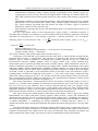
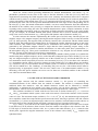
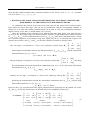
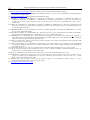
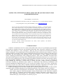
SISOM 2009 and Session of the Commission of Acoustics, Bucharest 28-29 May
SATELLITE ATTITUDE DYNAMICS USING EULER ANGLES 3D ROTATION
PARAMETERIZATION
Dan DUMITRIU, Cornel SECARĂ
Institute of Solid Mechanics, Romanian Academy, Str. Constantin Mille, nr. 15, 010141 Bucharest, Romania
Corresponding author: Dr.-Ing. Dan DUMITRIU, e-mail: [email protected]
Abstract: This paper studies the attitude/orientation dynamics of a CubeSat, i.e., a 10×10×10 cm cube
small satellite with the mass of 1 kg. The dynamics considerations presented here remain valid for
bigger satellites and for satellites of non-cubic forms. No atmospheric drag, solar radiation pressure or
other perturbations were considered in this paper. The attitude dynamics of the satellite with respect
to its center of mass is formulated using Euler angles 3D rotation parameterization. Based on the
direct dynamics formulation, an inverse dynamics approach has been developed as satellite
orientation guidance&control strategy, and will be presented in a future paper. The difficulty of the
case considered is the fact that the attitude control is performed using a two-axis momentum reaction
G
G
wheels system, so not all three axes are controlled, but only the xsat and y sat axes. If a three-axis
moment control based on inverse dynamics is quite trivial, our two-axis moment control is not
obvious at all, one can find always unfavorable cases when the proposed control strategy fails. The
two-axis moment control problem can occur also for a three-axis controlled satellite in the accidental
case when one moment thruster fails.
Keywords: CubeSat, Attitude Determination and Control, Direct Dynamics, 3D Rotation
Parameterization, Euler Angles.
1. INTRODUCTION
CubeSat is a standard 10×10×10 cm cube small satellite with a mass of 1 kg maximum, proposed since
1999 jointly by Stanford University and California Polytechnic State University (CalPoly) [1-3]. Briefly,
CubeSat can be defined as “1 liter, 1 kilogram, 1 Watt” [6], due to its small size associated with very low
energy consumption. The standardization of this miniaturized satellite (called also pico-satellite) is aimed to
reduce the launch costs and to induce a better collaboration between universities working on the same topics
and model. The first CubeSats were launched in 2003, and nowadays it is quite a popular tool for space
science technology demonstration, with pedagogical purposes. Thus, many worldwide universities have
developed CubeSat projects involving teams of students supervised by their professors. Let’s cite here just a
few most recent CubeSat projects [12] developed by different European universities and research centers:
Ecole Polytechnique Fédérale de Lausanne, Switzerland [4], University of Vigo, Spain [5], Université de
Liège, Belgium [6], University of Trieste, Italy [7], Narvik University College, Norway [8], Würzburg
University, Germany [9], Romanian Space Agency in collaboration with University of Bucharest and
University Politehnica of Bucharest [10-11]. Let’s cite also pico-satellites “XI-IV” and “XI-V” developed by
University of Tokio [13] and CanX-2 (Canadian Advanced Nanospace eXperiment 2) developed by the
Space Flight Laboratory at the University of Toronto Institute for Aerospace Studies [14].
Beside its pedagogical role, the main CubeSat space exploration purpose is to collect in-orbit scientific
information and to send this information to the Earth/ground station. The scientific issues are numerous:
- weather observation and atmospheric measurements: airglow phenomena [4], ionizing radiation [5],
solar weather, magnetic field and atmospheric density measurements in near Earth space radiation
environment [7], greenhouse gases detection using a miniature atmospheric spectrometer [14], inorbit temperature measurements [8], micrometeorite detection [10-11], cosmic radiation dose
measurement [11], GPS atmospheric occultation [14], etc;
Satellite Attitude Dynamics using Euler Angles 3D Rotation Parameterization
99
-
communication technology testing: software defined reconfigurable radio (SRAD) system [5],
communication protocol in space for D-STAR (Digital Smart Technology for Amateur Radio) [6],
VHF/UHF communication with the ground station [8-9], other amateur radio frequency experiments
[13];
- experimental validation of space navigation technology: solar panel deployment system [5], Attitude
Determination and Control Subsystem (ADCS) [8-9], formation-flying technology demonstration
[14], surface material experiment that will measure the effects of atomic oxygen on advanced
materials for satellites in low Earth orbit [14];
- Earth monitoring (taking Earth pictures and downloading them to the ground station [8,10-11,13])
and astronomy.
The new Vega launch vehicle of the European Space Agency (ESA) is scheduled to deploy, in
November 2009, a number of 9 CubeSats, on an orbit characterized by the following parameters, at least for
AtmoCube [7]: semi-major axis a = 7153.14 [km] , eccentricity e = 0.0594 , inclination i = 71° . It results the
3
following period T of the reference orbit: T = 2π a ≅ 6020.8 [s] ≅ 100.35 [min] , where μ = G ⋅ mEarth =
μ
3
= 3.986 ⋅ 106 [ km2 ] . It comes also:
s
- number of orbits/day = 14.3;
- ΔΩ (node shift/orbit due to Earth rotation) = -25.09 deg/orbit (-358.96 deg/day);
- average CubeSat velocity = 7.458 [km/s];
The average visibility at the ground station will be around 8 min [7,11].
Among the 9 CubeSats that will be deployed on this orbit, there is Goliat CubeSat developed by the
Romanian Space Agency in collaboration with University of Bucharest and University Politehnica of
Bucharest [10-12]. Goliat is planned to accomplish three scientific payloads [10-11]: low Earth orbit
micrometeorite detection (SAMIS platform based on impact sensors [11]), cosmic radiation dose
measurement (Dose-N experiment), Earth observation (CICLOP camera). Goliat satellite Bus consists of a
number of different subsystems [11]: Electrical Power Supply (EPS), Attitude Determination and Control
Subsystem (ADCS), Radio Communications (COMM), on-board computer, etc. Each of these customized
components fulfills a specific task in order to support the payloads of Goliat. For example, the power supply
of around 2 Watts is generated by solar cells/panels placed on the sides of the cube and there is also a
reloading battery as buffer for temporarily power peaks, i.e., if for some reason (eclipse, failure) the solar
panels don’t supply enough power [7,8,11-12]. In what concerns the ground stations which will ensure the
radio communications with the satellite, for Goliat there is one ground station in Bucharest and the second
one with a 4m dish telescope is located in Cluj-Napoca [11].
The camera mounted on a CubeSat should be able to take pictures of the Earth, pictures as clear as
possible, e.g., CICLOP camera mounted on Goliat has an expected picture area of 50×70 km, with a pixel
area of 21×28 m [11]. One should be able to discern between land and water (for example) on the
downloaded pictures. For that, it is a must to have a good stability of the camera (so of the CubeSat) and the
appropriate orientation, all this in the hazardous and perturbed orbital environment. If the CubeSat is not
stable, then the pictures will show us a blurred image of the area the picture has taken [4,8].
This paper concerns the attitude dynamics and control of the satellite, which is part of the Attitude
Determination and Control Subsystem (ADCS) payload, where position, velocity and orientation are
determined and controlled. In terms of control, the ADCS shall perform [4,8]: 1) detumbling after launch or
after some free-flying period, i.e., to reduce the angular velocity (spinning rate) of the satellite to a minimum;
2) attitude stabilization, i.e., maintaining an existing orientation; 3) attitude maneuver control, i.e., to
orientate the satellite from a current/initial attitude to the attitude desired for taking pictures or for some other
action.
The ADCS determines and actively controls the attitude of the satellite, using: a) appropriate sensors to
provide feedback on satellite orientation; b) an actuator mechanism to implement the control; c) the on-board
computer microcontroller unit, which receives the sensor measurements, then determines the attitude and
finally computes the control signals. The control can also be commanded from the ground station.
Dan DUMITRIU, Cornel SECARĂ
100
There are various sensors providing information for attitude determination: sun sensors, e.g., six
photodiodes positioned on the sides of the cube to find the direction of the Sun [8,11-12]; three-axis
magnetometers measuring the Earth magnetic field vector (intensity and direction) that will be compared
with the model [3,4,8,9,11,14]; three-axis gyroscope to measure the spinning rate for each axis (needed for a
correct propagation of the attitude data) [4,9,11]; a nanospacecraft-sized star tracker [14], etc. The currents
produced by the solar cells can also provide information about the solar angle on the corresponding side of
the cube [8,13]. Once the attitude information available, one must extract/determine from this information
the attitude of the satellite, more precisely to compute the direction of the magnetic field and of the sun
according to the position along the orbit. This attitude determination is quite a complex estimation; it needs
different algorithms and models, such as a propagator, an Earth's magnetic field model, a sun vector model,
etc [4]. For example, an Extended Kalman Filter (EKF) estimator can be used for attitude determination,
using a time series of measurements (e.g., GPS signals) and dynamic and/or kinematic models [15].
In what concerns the actuators implementing the control part of ACDS, many CubeSat projects use
magnetic torque coils (magneto-torquers) which generate the magnetic fields necessary to orient the satellite
[3,4,7,8]. More precisely, the magnetic field provided by current in the coil interacts with the Earth's natural
magnetic field, thus producing the resultant torque for orienting the satellite. Magneto-torquers are not really
active actuators; they rather realize efficient passive stabilization and control, provided that the torque
generated by the permanent magnets should be larger than the other perturbing torques acting on the
CubeSat. Another passive solution for satellite stabilization is to take some profit from a perturbation, i.e.,
the atmospheric drag [16]. These passive stabilization solutions are very frequent for low altitude satellite
missions, because of their reduced cost and power consumption.
Several actuator system choices can be made, following the attitude control payload: a) to stabilize the
satellite using three magneto-torquers, one for each of the three orthogonal axes of the CubeSat [3]; b) to use
only two magneto-torquers to passively stabilize two of the CubeSat axes [7], and for the third axis one or
two momentum wheels can possibly be used as active actuators [9,12,14]; c) or to use three active actuators,
e.g., momentum reaction wheels, one active actuator per each satellite axis [14]. Other choices are possible,
e.g., Goliat uses only a two momentum wheels actuation system, to control its 3D attitude motion [11]. This
case will be studied here. The “handicap” of controlling only two axes for a 3D rotation motion must be
bypassed using an appropriate control. This two-axis control case of an underactuated satellite is very
interesting, since this special situation can occur even for three-axis controlled satellites in the accidental
case when one moment thruster fails.
2. SATELLITE ATTITUDE DYNAMICS PROBLEM
This paper concerns only the attitude maneuver control, i.e., the process of controlling the
reorientation/rotation of the satellite from one attitude to another. The satellite is considered already
stabilized before this maneuver. Also, the attitude maneuver control can be followed by “attitude
stabilization” to maintain the new attitude [4,8]. More precisely, only the direct dynamics formulation is
presented here, while an inverse dynamics control technique will be presented in a future paper.
The actuation considered is similar with the one conceived on Goliat CubeSat [11], i.e., a two axes
G
G
( xsat and y sat ) momentum wheels system, where each micro-motor is fixed in the structure’s hole, from the
center of a face. The maximum torque available is Tmax = 0.12 ⋅ 10-3 [N ⋅ m] , the minimum torque being null.
Servo amplifiers control the torque and the speed between the limits, allowing to perform a full 360º rotation
in around 40 s [11]. Since no magneto-torquers where used as actuators, but momentum reaction wheels, no
interaction between the CubeSat satellite and Earth’s magnetic field was considered in this paper.
Fig. 1 shows a view from above the orbital plane, indicating the orthogonal axes of the Local Vertical
Local Horizon (LVLH) reference frame used to locate the satellite with respect to the reference orbit. The
G
G
LVLH origin is located on the reference orbit; z LVLH points in the nadir direction; y LVLH is normal to the
G
orbital plane, opposite the angular momentum vector of the reference orbit; finally, x LVLH completes the
right-hand frame.
101
Satellite Attitude Dynamics using Euler Angles 3D Rotation Parameterization
Fig. 1. View of the orbital plane, with the Local Vertical Local Horizon (LVLH) inertial reference frame
G
G
G
Fig. 2 shows the CubeSat and its body frame (with the origin in O and with xsat , y sat and z sat as body
axes), as well as the axes of LVLH which is the “fixed”, inertial frame with respect to whom the body frame
will be located. For simplification, the gravity center G of the satellite was considered as coincident with the
G
geometric center of the cube O, i.e., G≡O. The axis z sat of the body frame is oriented on the direction of the
G
G
camera objective, while xsat and y sat axes coincide with the direction of positive torques Tx and Ty produced
by the two momentum reaction wheels actuating the CubeSat. The desired attitude for taking pictures will
G
G
G
G
G
G
correspond to xsat = x LVLH , y sat = y LVLH and z sat = z LVLH (nadir direction), i.e., null Euler angles for the
orientation of the body frame with respect to LVLH (see next section for details of Euler angles 3D rotation
parameterization).
Fig. 2. View of the CubeSat with its body axes, compared with LVLH axes
CubeSat is a standard 10×10×10 cm cube small satellite; its mass is around m = 1 [kg] and the
following symmetric moment of inertia tensor with respect to the body frame was considered here:
⎡ J xx
⎢
J = ⎢ J xy
⎢ J xz
⎣
J xy
J yy
J yz
J xz ⎤ ⎡16.51
0
0 ⎤
⎥ ⎢
J yz ⎥ = ⎢ 0
16.51
0 ⎥⎥ [kg ⋅ cm 2 ] .
J zz ⎥⎦ ⎢⎣ 0
0
16.80 ⎥⎦
(1)
The moment of inertia tensor is approximated as constant in time, considering the momentum reaction
wheels as moving bodies perfectly centered when rotating around their actuation axis. The form of J in (1)
Dan DUMITRIU, Cornel SECARĂ
102
G
G
shows that the satellite considered has a symmetric structure on xsat and y sat axes, i.e., J xx = J yy , and there
is no cross term, i.e., J xy = J xz = J yz = 0 .
3. EULER ANGLES 3D ROTATION PARAMETERIZATION OF CUBESAT’S BODY FRAME
WITH RESPECT TO THE INERTIAL LVLH REFERENCE FRAME
To parameterize the position of the body frame with respect to the inertial LVLH reference frame,
Euler angles are used in this paper. One can also use quaternions, with the corresponding equations of
motion [3,17,19]. Other 3D rotation parameterizations can be used as well, such as Rodrigues parameters,
angular velocity vector, full 3×3 rotation matrix, etc [17,22-24].
Thus, the orientation of the CubeSat can be defined using three Euler angles (roll, pitch and yaw)
[3,15-19,22-25]. These Euler angles are obtained from the sequence of right hand positive rotations from the
G
G
G
G G G
( x LVLH , y LVLH , z LVLH ) LVLH orthonormal basis to the ( xsat , y sat , z sat ) body frame orthonormal basis. Among
the 12 possible sequences of 3D rotations using Euler angles [25], the x-y-x (roll-pitch-roll) sequence was
G
G
chosen to be used here, since xsat and y sat are the only CubeSat axes which are actuated. Thus:
0
0 ⎤
⎡1
⎢
• the roll angle α corresponds to a first x-axis elementary rotation matrix R α = ⎢0 cos α − sin α ⎥⎥
⎢⎣0 sin α cos α ⎥⎦
G
G
G
describing the transformation between the orthonormal basis ( x LVLH , y LVLH , z LVLH ) and the intermediate
G
G G
orthonormal basis ( x LVLH , y1 , z1 ), i.e.
G
G
G
G
y LVLH = R α y1 and z LVLH = R α z1 ;
⎡ cos β 0 sin β ⎤
• the pitch angle β corresponds to a second y-axis elementary rotation R β = ⎢⎢ 0
1
0 ⎥⎥ describing
⎢⎣ − sin β 0 cos β ⎥⎦
G
G G
the transformation between the intermediate orthonormal basis ( x LVLH , y1 , z1 ) and another intermediate
G G G
orthonormal basis ( xsat , y1 , z 2 ), i.e.
G
G
G
G
x LVLH = R β xsat and z1 = R β z 2 ;
0
0 ⎤
⎡1
⎢
⎥
• finally, the roll angle γ corresponds to a third x-axis elementary rotation R γ = 0 cos γ − sin γ
⎢
⎥
⎣⎢0 sin γ cos γ ⎦⎥
G G G
describing the transformation between the intermediate orthonormal basis ( xsat , y1 , z 2 ) and the body
G G G
frame orthonormal basis ( xsat , y sat , z sat ), i.e.
G
G
G
G
y1 = R γ y sat and z 2 = R γ z sat .
Based on this x-y-x (roll-pitch-roll) Euler angles parameterization, appropriate for the studied case where
G
G
xsat and y sat are the only actuated axes, the attitude matrix A is computed as follows [25]:
0
0 ⎤ ⎡ cos β 0 sin β ⎤ ⎡1
0
0 ⎤
⎡1
⎢
⎥
⎢
⎥
⎢
A = R α R β R γ = ⎢ 0 cos α − sin α ⎥ ⎢ 0
1
0 ⎥ ⎢0 cos γ − sin γ ⎥⎥ =
⎣⎢ 0 sin α cos α ⎦⎥ ⎣⎢ − sin β 0 cos β ⎦⎥ ⎣⎢0 sin γ cos γ ⎦⎥
sin β sin γ
sin β cos γ
⎡ cos β
⎤
⎢
= ⎢ sin α sin β cos α cos γ − sin α cos β sin γ − cos α sin γ − sin α cos β cos γ ⎥⎥
⎢⎣ − cos α sin β sin α cos γ + cos α cos β sin γ − sin α sin γ + cos α cos β cos γ ⎥⎦
(2)
103
Satellite Attitude Dynamics using Euler Angles 3D Rotation Parameterization
This attitude matrix A transforms an arbitrary vector v from the satellite body frame coordinates to the orbitdefined LVLH coordinates: v LVLH = A v sat . That’s why it is also called 3×3 direction cosine matrix from
body frame coordinates to inertial LVLH coordinates. In particular, A transforms the moving axes of the
G
G
G
G
G
G
body frame into the “fixed” axes of LVLH, i.e.: x LVLH = A xsat , y LVLH = A y sat and zLVLH = A zsat .
The singularities associated to Euler angles parameterizations are well-known, e.g., in our x-y-x case if
G
G
β is a multiple of π, then x LVLH and xsat coincide, and the rotations of angles α and γ are getting superposed
G
G
in a single rotation of angle α±γ around the same axis xsat = x LVLH . In this singular case, only the sum of α
and γ or their difference matters, thus there is an infinity of solutions α and γ for obtaining the concerned
rotation [23]. So, when working with Euler angles parameterizations, one has always to deal with these
singularities and be careful to avoid their negative effect on solving the equations of motion.
From (2), it comes easily the derivative of the attitude matrix:
⎡
⎢
−β sinβ
⎢
⎢
⎢
= ⎢α
cos αsinβ+β sin αcosβ
A
⎢
⎢
⎢
⎢α
sin αsinβ−β cos αcosβ
⎢
⎣
β cosβsin γ +γ sinβcos γ
sin αcos γ −γ cos αsin γ −α cosαcosβsin γ
−α
+β sin αsinβsin γ −γ sin αcosβcos γ
cosαcos γ −γ sin αsin γ −α
sin αcosβsin γ
α
−β cos αsinβsin γ +γ cos αcosβcos γ
⎤
⎥
⎥
⎥
α sin αsin γ −γ cos αcos γ −α cos αcosβcos γ ⎥
⎥
+β sin αsinβcos γ +γ sin αcosβsin γ
⎥
⎥
⎥
cosαsin γ −γ sin αcos γ −α
sin αcosβcos γ⎥
−α
⎥
−β cos αsinβcos γ −γ cosαcosβsin γ
⎦
β cosβcos γ −γ sinβsin γ
Let us calculate now the angular velocity tensor j(ω) as [20,23]:
= (R R R )T A
= RT RT RT A
j(ω) = A T A
α β γ
γ β α
⎡
0
−(α sin β cos γ − β sin γ ) α sin β sin γ + β cos γ ⎤
⎢
⎥
0
= ⎢ α sin β cos γ − β sin γ
−(α cos β + γ ) ⎥
⎢ −(α sin β sin γ + β cos γ )
⎥
0
α cos β + γ
⎣
⎦
(3)
where ω = [ ω1 ω2 ω3 ] is the angular velocity vector referenced with respect to the inertial LVLH frame,
but expressed in body frame coordinates [15,23], and the linear mapping j(ω) is nothing else than the cross
product on the left by ω, it has the following skew-symmetric form:
T
⎡ 0
j(ω) = ⎢⎢ ω3
⎢⎣ −ω2
−ω3
0
ω1
ω2 ⎤
⎥
−ω1 .
⎥
0 ⎥⎦
(4)
G G G
By identification between (3) and (4), one obtains the components in the body frame (O; xsat , y sat , z sat ) of the
angular velocity vector ω [16-19,21]:
⎧ω1 = α cos β + γ
⎪
⎨ω2 = α sin β sin γ + β cos γ
⎪
⎩ω3 = α sin β cos γ − β sin γ
(5)
Dan DUMITRIU, Cornel SECARĂ
104
4. CUBESAT ATTITUDE DYNAMICS USING EULER’S EQUATION OF MOTION
The rotation motion of a rigid body is generated by the torques applied on this body. For CubeSat, the
only torques considered here are the two torques produced by the two momentum reaction wheels used as
G G G
actuators, gathered in the torque vector T expressed in the body frame (O; xsat , y sat , z sat ) as
⎡Tx ⎤
G
G
T = Tx xsat + Ty y sat = ⎢⎢Ty ⎥⎥ .
⎢⎣ 0 ⎥⎦
(6)
In-orbit perturbations acting on CubeSat, e.g., atmospheric drag or solar radiation pressure, are neglected in
this paper. So, there is no torque generated by the in-orbit perturbation forces.
G G G
Considered with respect to the inertial LVLH frame, but expressed in the body frame (O; xsat , y sat , z sat ),
Euler’s equation of motion for the CubeSat relates the time derivative of the angular momentum vector
H = J ω to the torque vector T [3,15-16,18-21]:
T=
dH
.
= Jω
dt
(7)
where it was considered that J = 0 , for the considered J given by (1).
By derivation of (5), one obtains the time derivative of the angular velocity vector:
⎧ω
1 = α
cos β + γ − αβ
sin β
⎪⎪
cos γ + αβ
sin γ
2 =α
sin β sin γ + β
cos β sin γ + αγ
sin β cos γ − βγ
⎨ω
⎪
sin γ + αβ
cos γ
sin β cos γ − β
cos β cos γ − αγ
sin β sin γ − βγ
⎪⎩ω3 = α
(8)
= J −1T , provides:
Taking into account the expression (8) of ω, Euler’s equation of motion (7), rewritten as ω
⎧α
cos β + γ − αβ
sin β = (J −1T)1
⎪⎪
cos γ + αβ
sin γ = (J −1T)
sin β sin γ + β
cos β sin γ + αγ
sin β cos γ − βγ
⎨α
2
⎪
−1
⎪⎩α sin β cos γ − β sin γ + αβ cos β cos γ − αγ sin β sin γ − βγ cos γ = (J T)3
(9)
where J −1 stands for the inverse of the moment of inertia tensor J and where (J −1T)i , i=1,2,3 is the i-th
component of J −1T vector.
and γ :
, β
From (9), one obtains easily the explicit expressions of α
⎧α
−1
−1
1
⎪ = sin β [(J T) 2 sin γ + (J T)3 cos γ − αβ cos β + βγ ]
⎪⎪
= ( J −1T) cos γ − (J −1T) sin γ − αγ
sin β
⎨β
2
3
⎪
] + α β
⎪γ = (J −1T)1 − cos β [(J −1T) 2 sin γ + (J −1T)3 cos γ + βγ
sin β
sin β
⎪⎩
(10)
These expressions (10) are the differential equations characterizing the direct dynamics of CubeSat’s
attitude. It is easy to integrate (10) using for example Runge-Kutta integration methods.
In the considered case where the moment of inertia tensor J has the form (1), so
Ty
T
J −1 = diag( 1 , 1 , 1 ) , and for the torque vector T given by (6), then (J −1T)1 = x , (J −1T) 2 =
and
J xx J yy J zz
J xx
J yy
(J −1T)3 = 0 , and the differential equations (10) simplify as follows:
105
Satellite Attitude Dynamics using Euler Angles 3D Rotation Parameterization
⎧
⎛T
⎞⎟
= 1 ⎜ y sin γ − αβ
cos β + βγ
⎪α
J
sin
β
⎝ yy
⎠
⎪
⎪
⎪ Ty
sin β
⎨β = J cos γ − αγ
yy
⎪
⎪
⎛T
T
⎞⎟ + αβ
⎪γ = x − cos β ⎜ y sin γ + βγ
J xx sin β ⎝ J yy
⎪⎩
⎠ sin β
(11)
CubeSat direct dynamics results based on the Runge-Kutta numerical integration of the differential
equations (10) involving the Euler angles will be presented in next subsection.
5. SOME ATTITUDE CONTROL RESULTS OBTAINED USING AN INVERSE DYNAMICS
TECHNIQUE
To show some direct dynamics results, obtained by solving the differential equations (11), one needs to
use some control law, i.e., some evolution for the torques Tx and Ty . In fact, an attitude control technique
based on inverse dynamics of (10)-(11) is already in-testing. The results presented below are obtained using
the control law provided by our attitude control technique, which will be presented in a future paper.
Let’s recall that the purpose of the attitude maneuver control is to rotate the satellite from an initial
attitude at time tin, characterized by the Euler angles (αin , βin , γ in ) , to the final time tf desired attitude
characterized by (α f , βf , γ f ) . The satellite is considered already stabilized before this maneuver, i.e.,
α in ≅ 0 , β in ≅ 0 , γ in ≅ 0 . At the end tf of the maneuver, the satellite should have null velocity, i.e., α f ≅ 0 ,
β f ≅ 0 , γ f ≅ 0 , and should be oriented towards the Earth in order to take pictures, i.e., α f ≅ 0 , βf ≅ 0 ,
G
G
G
G
G
G
γ f ≅ 0 ( z sat must coincide with z LVLH , and we will also impose xsat = x LVLH and y sat = y LVLH ).
To perform this rotation maneuver in Δtmaneuv = tf − tin seconds, the satellite considered in this paper
G
G
disposes of active control torques only on two axes, more precisely of Tx on xsat axis and of Ty on y sat axis.
Table 1 shows two cases of attitude control maneuver (Case 1 and Case 2), successfully performed, both for
Δtmaneuv = 100 [s] .
Table 1. Satellite final state tf for Case 1 and 2 of attitude control
Case 1
Case 2
αin [°]
-117.74
131.62
βin [°]
172.71
-96.35
γin [°]
-82.29
109.76
Fig. 3 shows the direct dynamics results, as well as the torques which produced Case 1 direct dynamics
results. Fig. 4 shows Case 2 direct dynamics results with the corresponding torques.
Fig. 3. Case 1 results in what concerns the Euler angles and the corresponding torques to obtain Case 1 direct dynamics
Dan DUMITRIU, Cornel SECARĂ
106
Fig. 4. Case 2 results in what concerns the Euler angles and the corresponding torques to obtain Case 2 direct dynamics
One can see that in Case 1 and 2 the attitude control maneuver was successfully performed. But there are still
cases where the maneuver is not converging, so there is still work to do before proposing in the next paper a
reliable attitude control technique based on inverse dynamics.
5. CONCLUSIONS AND FUTURE WORK
After an extended introduction trying to present general considerations about different CubeSat
projects, this paper develops the differential equations which are governing the attitude dynamics of a
CubeSat. A usual Euler angles parameterization was used to represent the 3D rotation of the satellite. Based
on the direct dynamics formulation, an inverse dynamics approach can be used as control technique for
performing attitude control maneuver. Improving such a control technique is an ongoing work and will be
presented in a future paper. The purpose is to have a reliable Attitude Determination and Control Subsystem
(ADCS), able to rotate on command the satellite to a desired attitude, and keep it in that attitude.
The particularity of the considered attitude control problem is that only two axes of the satellite are
actuated, not all three. So, one deals with an under-actuated system where the difficulty is to control different
3D rotations using only two actuators for three degrees of freedom. This two-axis moment control problem
can occur for a three-axis controlled satellite in the accidental case when one moment thruster fails. So, the
study of this two-axis only active control case is very important for a majority of satellite missions.
ACKNOWLEDGEMENT. The authors gratefully acknowledge the National Authority for Scientific
Research (ANCS, UEFISCSU), for financial support through PN-II project nr. 106/2007, code ID_247/2007.
The authors thank Dr.-Ing. Boris CONONOVICI, Dr.-Ing. Ion NIŢU and the colleagues from the
Mechatronics Department at the Institute of Solid Mechanics, for useful insights and discussions on the
topics of this paper.
REFERENCES
1. http://en.wikipedia.org/wiki/Cubesat
2. http://www.cubesat.org/
3. KRISHNAMURTHY, N., Dynamic Modelling of CubeSat Project MOVE, Master Thesis, Luleå University of Technology,
Sweden, 2008.
4. http://swisscube.epfl.ch/ (Swisscube CubeSat project developped by Ecole Polytechnique Fédérale de Lausanne)
5. http://www.xatcobeo.com/ (Xatcobeo CubeSat project developed by University of Vigo)
6. http://www.leodium.ulg.ac.be/cmsms/ (Oufti-1 CubeSat project developed by Université de Liège)
7. http://www2.units.it/~atmocube/ (AtmoCube Cubesat project developed by University of Trieste)
8. http://hincube.hin.no/ (Hincube Cubesat project developed at Narvik University College, Norway)
9. http://www7.informatik.uni-wuerzburg.de/ (UWE-3 CubeSat project developed by Würzburg University)
107
Satellite Attitude Dynamics using Euler Angles 3D Rotation Parameterization
10. http://ro.wikipedia.org/wiki/GOLIAT (Goliat CubeSat project developed by Romanian Space Agency)
11. Mugurel BĂLAN et al. (Romanian CubeSat Project members), GOLIAT – project overview (presentation), CubeSat Developers'
Workshop, 9-10 August 2008.
12. http://forum.spacealliance.ro/ (Space technology and education portal)
13. FUNASE, R., TAKEI, E., NAKAMURA, Y., NAGAI, M., ENOKUCHI, A., YULIANG, C., NAKADA, K., NOJIRI, Y.,
SASAKI, F., FUNANE, T., EISHIMA, T., NAKASUKA, S., Technology demonstration on University of Tokyo’s picosatellite “XI-V” and its effective operation result using ground station network, Acta Astronautica, 61, 7-8, pp. 707-711,
October 2007
14. SARDA, K., EAGLESON, S., CAILLIBOT, E., GRANT, C., KEKEZ, D., PRANAJAYA, F., ZEE, R.E., Canadian advanced
nanospace experiment 2: Scientific and technological innovation on a three-kilogram satellite, Acta Astronautica, 59, 1-5, pp.
236-245, July-September 2006.
15. PURIVIGRAIPONG, S., Spacecraft Attitude Estimations Using Phase Information of GPS Signals, Thammasat Int. J. Sc. Tech.,
8, 1, pp. 44-53, January-March 2003.
16. BOLANDI, H., BADPA, A., NASIRI SARVI, M., Application of passive gg-aero stabilization for near-Earth small satellites,
Iranian Journal of Information Science & Technology, 3, 1, pp. 57-71, January-June 2005.
17. RODRIGUES, D.S.S., ZANARDI, M.C., Spacecraft Attitude Propagation with Different Representations, In : Advances in
Space Dynamics 4: Celestial Mechanics and Astronautics (editor H.K. Kuga), pp. 143-150, Instituto Nacional de Pesquisas
Espaciais – INPE, São José dos Campos, SP, Brazil, 2004.
18. KANG J-Y, SHIN, K-K, Analysis of the Antenna Pointing Instability of a Satellite in Spin-Stabilized Injection Mode, ETRI
Journal, 16, 2, pp. 27-41, July 1994.
19. IZZO, D., BEVILACQUA, R., VALENTE, C., Optimal large reorientation manoeuvre of a spinning gyrostat, 6th Cranfield
Conference on Dynamics and Control of Systems and Structures in Space: 2004, Cranfield University Press, Bedfordshire,
UK, 2004, pp. 607-616.
20. STUCK, B.W., Solar Pressure Three-Axis Attitude Control, Journal of Guidance and Control, 3, 2, pp. 132-139, 1980.
21. WIE, B., Solar Sail Attitude Control and Dynamics, Part 1 & Part 2, Journal of Guidance, Control, and Dynamics, 27, 4, pp.
526-535 (Part 1), pp. 536-544 (Part 2), July-August 2004.
22. GOGU, G., COIFFET, Ph., Représentation du mouvement des corps solides, Editions Hermès, Paris, 1996.
23. DUMITRIU, D., Modélisation dynamique des systèmes articulés par des vecteurs translation et des matrices rotation. Prise en
compte des rigidités par des multiplicateurs de Lagrange. Simulations du mouvement à l’aide d’un code en C++, Ph.D.
thesis, University of Poitiers, France, 2003.
24. SPRING, K.W., Euler parameters and the use of quaternion algebra in the manipulation of finite rotations : A review,
Mechanism and Machine Theory, 21, 5, pp. 365-373, 1986.
25. http://en.wikipedia.org/wiki/Euler_angles