Download DSSAT User's Guide Vol. 3 - Projetos e Redes do Macroprograma 1

DSSAT
version 3
VOLUME 3
A Decision Support System
for Agrotechnology Transfer
Volume 3
DSSAT version 3
Editors:
Gordon Y. Tsuji
Goro Uehara
Sharon Balas
International Benchmark Sites Network for Agrotechnology Transfer
University of Hawaii, Honolulu, Hawaii
IBSNAT, The International Benchmark Sites Network for Agrotechnology
Transfer, is a network consisting of the contractor (University of Hawaii),
its subcontractors and many global collaborators. Together they have
created a network of national, regional and international agricultural
research for the transfer of agrotechnology among global partners in both
developed and lesser developed countries.
From 1982 to 1987, IBSNAT was a program of the U.S. Agency for
International Development under a cost-reimbursement Contract, No.
DAN-4054-C-00-2071-00, with the University of Hawaii. From 1987 to
1993, the contract was replaced with a Cooperative Agreement, No.
DAN-4054-A-00-7081-00, between the University of Hawaii and USAID.
Correct Citation: G.Y. Tsuji, G. Uehara and S. Balas (eds.). 1994.
DSSAT v3. University of Hawaii, Honolulu, Hawaii.
Copyright  University of Hawaii 1994
All reported opinions, conclusions and recommendations are those of the authors
(contractors) and not those of the funding agency or the United States govern-
LIBRARY
OF
CONGRESS 94-19296
ISBN 1-886684-03-0 (VOLUME 3)
ISBN 1-886684-00-6 (3 VOLUME SET)
D S S AT
V3
VOLUME 3
VOLUME 3-1
S E A S O N A L A N A LY S I S
VOLUME 3-2
S E Q U E N C E A N A LY S I S
VOLUME 3-3
W E AT H E R M A N
VOLUME 3-4
GENOTYPE COEFFICIENT
C A L C U L AT O R
DSSAT v3, Volume 3
iv
•
DSSAT v3, Volume 3
•
DSSAT v3, Volume 3
•
DSSAT v3, Volume 3
•
DSSAT v3, Volume 3
•
DSSAT v3, Volume 3
•
DSSA
TABLE OF CONTENTS
VOLUME 3-1.
CHAPTER ONE.
S E A S O N A L A N A LY S I S
1
INTRODUCTION
3
SYSTEM REQUIREMENTS
CHAPTER TWO.
4
CREATING MODEL INPUT FILES
FOR
SEASONAL
ANALYSIS
CHAPTER THREE.
5
RUNNING SEASONAL ANALYSIS EXPERIMENTS
13
OVERVIEW
13
AN EXAMPLE
14
INFORMATION
CHAPTER FOUR.
AND
ERROR MESSAGES
17
ANALYZING SEASONAL ANALYSIS EXPERIMENTS
23
OVERVIEW
23
AN EXAMPLE
24
ANALYZE BIOPHYSICAL VARIABLES
26
GRAPHICS MAIN MENU
28
ANALYZE ECONOMIC VARIABLES
34
ECONOMIC EVALUATION MAIN MENU
34
MODIFY HARDCOPY OPTIONS
44
SELECTING ANOTHER INPUT FILE
INFORMATION
AND
FOR
ANALYSIS
ERROR MESSAGES
48
REFERENCES
APPENDIX A.
55
COMBINING YIELD
AND
PRICE DISTRIBUTIONS
AN ILLUSTRATION
APPENDIX B.
48
THREE DECISION CRITERIA
57
58
59
MEAN-VARIANCE (EV) ANALYSIS
59
STOCHASTIC DOMINANCE (SD) ANALYSIS
59
MEAN-GINI DOMINANCE (MGD) ANALYSIS
60
AN EXAMPLE
60
¥ DSSAT v3, Volume 3 ¥ DSSAT v3, Volume 3 ¥ DSSAT v3, Volume 3 ¥ DSSAT v3, Volume 3 ¥ DSSAT v3, Volume 3 ¥ DSSAT v3, Volume 3 ¥ DSSAT v3, Volume
v
FIGURES
FIGURE 1. STEPS
IN
SEASONAL ANALYSIS
FIGURE 2. MENU OPTIONS
FOR THE
4
SEASONAL ANALYSIS PROGRAM
23
FIGURE 3. STOCHASTIC PRICE-COST DISTRIBUTIONS
38
TABLES
TABLE 1. SEASONAL EXPERIMENT LISTING FILE EXP.LST
5
TABLE 2. PART
7
OF
MODEL INPUT FILE UFGA7812.SNX
TABLE 3. SUMMARY OUTPUT LISTING FILE SEASONAL.LST
13
TABLE 4. SUMMARY OUTPUT FILE UFGA7812.SNS (FIRST 20
DATA RECORDS ONLY)
18
TABLE 5. PRICE-COST FILE DEFAULT.PRI
37
TABLE 6. SAMPLE SECTION
45
OF
GRAPH.INI
TABLE 7. PRINTER TYPES SUPPORTED
GRAPHICS PROGRAM
46
TABLE 8. EXPERIMENT DATA CODES FILE DATA.CDE – SUMMARY
SECTION ONLY
47
TABLE 9. PART
DSSAT v3, Volume 3
vi
•
DSSAT v3, Volume 3
OF
•
BY THE
SEASONAL ANALYSIS RESULTS FILE UFGA7812.SNR 4 9
DSSAT v3, Volume 3
•
DSSAT v3, Volume 3
•
DSSAT v3, Volume 3
•
DSSAT v3, Volume 3
•
DSSA
VOLUME 3-2.
CHAPTER ONE.
S E Q U E N C E A N A LY S I S
67
INTRODUCTION
69
SYSTEM REQUIREMENTS
CHAPTER TWO.
70
CREATING MODEL INPUT FILES
FOR
SEQUENCE
ANALYSIS
FILEX
FOR
73
SEQUENCE ANALYSIS
73
TIMING CONTROLS
78
SIMULATION CONTROL OPTIONS
79
CHAPTER THREE.
RUNNING SEQUENCE ANALYSIS EXPERIMENTS
81
OVERVIEW
81
AN EXAMPLE
82
INFORMATION
CHAPTER FOUR.
AND
ERROR MESSAGES
84
ANALYZING SEQUENCE ANALYSIS EXPERIMENTS
89
OVERVIEW
89
AN EXAMPLE
90
ANALYZE BIOPHYSICAL VARIABLES
93
GRAPHICS-REGRESSION MAIN MENU
96
ANALYZING MORE
THAN
ONE CROP
AT A
TIME
107
ANALYZE ECONOMIC VARIABLES
112
ECONOMIC EVALUATION MAIN MENU
112
MODIFY HARDCOPY OPTIONS
121
SELECTING ANOTHER INPUT FILE
INFORMATION
AND
FOR
ANALYSIS
126
ERROR MESSAGES
126
REFERENCES
APPENDIX.
133
THE STABILITY
OF
OUTPUT VARIABLES
FROM
REPLICATED SEQUENCE EXPERIMENTS
135
FIGURES
FIGURE 1. STEPS
IN
SEQUENCE ANALYSIS
FIGURE 2. MENU OPTIONS
FOR THE
SEQUENCE ANALYSIS PROGRAM
71
90
¥ DSSAT v3, Volume 3 ¥ DSSAT v3, Volume 3 ¥ DSSAT v3, Volume 3 ¥ DSSAT v3, Volume 3 ¥ DSSAT v3, Volume 3 ¥ DSSAT v3, Volume 3 ¥ DSSAT v3, Volume
vii
FIGURE 3. “SIMULATED” SEQUENCE OUTPUTS
AND
FOR
N = 100, 20, 10,
5, RESPECTIVELY.
136
TABLES
TABLE 1. SEQUENCE EXPERIMENT LISTING FILE EXP.LST
TABLE 2. A SAMPLE FILEX
FOR
73
CROP SEQUENCING: EBAF1101.SQX 7 5
TABLE 3. SUMMARY MODEL OUTPUT LISTING FILE SEQUENCE.LST
81
TABLE 4. SUMMARY OUTPUT FILE EBAF1101.SQS (FIRST 20
DATA RECORDS ONLY)
TABLE 5. PART
OF THE
85
DEFAULT SEQUENCE PRICE FILE, DEFAULT.PRQ 1 1 5
TABLE 6. SAMPLE SECTION
OF
GRAPH.INI
TABLE 7. PRINTER TYPES SUPPORTED
BY THE
123
GRAPHICS PROGRAM
124
TABLE 8. EXPERIMENT DATA CODES FILE DATA.CDE – SUMMARY
SECTION ONLY
TABLE 9. PART
DSSAT v3, Volume 3
viii
•
DSSAT v3, Volume 3
OF
•
125
SEQUENCE ANALYSIS RESULTS FILE EPAF1101.SQR 1 2 7
DSSAT v3, Volume 3
•
DSSAT v3, Volume 3
•
DSSAT v3, Volume 3
•
DSSAT v3, Volume 3
•
DSSA
VOLUME 3-3.
CHAPTER ONE.
W E AT H E R M A N
INTRODUCTION
137
139
PROGRAM DESCRIPTION
139
OVERVIEW
140
OF
FUNCTIONS
SYSTEM REQUIREMENTS
CHAPTER TWO.
140
GETTING STARTED
141
STARTING WEATHERMAN
141
WEATHERMAN USER INTERFACE
141
COMMON DIALOG BOXES
144
STEPS
FOR
CLEANING
CHAPTER THREE.
AND
INTRODUCTORY TUTORIAL
BROWSE
THE
SELECT
NEW STATION
A
CONVERTING WEATHER DATA
MENU
AND
ONLINE HELP
147
149
149
149
IMPORT DAILY WEATHER FILES
150
CALCULATE WEATHER GENERATOR PARAMETERS
152
GENERATE WEATHER DATA
152
CALCULATE STATISTICS
153
CALCULATE STATISTICS
FOR THE
GENERATED DATA
GRAPH OBSERVED DAILY TEMPERATURE
GRAPH STATISTICS
FOR
OBSERVED
AND
153
GENERATED DATA
EXPORT DAILY WEATHER FILES
CHAPTER FOUR.
153
WEATHERMAN REFERENCE GUIDE
154
155
157
VARIABLES
157
FILE MENU
157
STATION MENU
160
IMPORT/EXPORT MENU
164
GENERATE MENU
173
ANALYZE MENU
179
OPTIONS MENU
186
QUIT MENU
192
¥ DSSAT v3, Volume 3 ¥ DSSAT v3, Volume 3 ¥ DSSAT v3, Volume 3 ¥ DSSAT v3, Volume 3 ¥ DSSAT v3, Volume 3 ¥ DSSAT v3, Volume 3 ¥ DSSAT v3, Volume
ix
REFERENCES
193
APPENDIX A.
ABBREVIATIONS USED
WEATHERMAN
IN
195
DAILY WEATHER VARIABLES
195
SUMMARY FILES
195
APPENDIX B.
CLIMATE FILE FORMAT
197
TABLES
TABLE 1. USER INTERFACE ITEMS
AND THEIR
FUNCTIONS
IN
WEATHERMAN
TABLE 2. LIST
OF
142
ESSENTIAL STEPS
WEATHER DATA FILE
FROM
RAW DATA
IN
FOR
CREATING
WITH THE
COMPLETE DAILY
A
CORRECT FORMAT
AND
UNITS
WEATHERMAN
TABLE 3. WEATHERMAN VARIABLES
AND
148
ASSOCIATED UNITS
TABLE 4. WEATHER STATION INFORMATION REQUIRED
FOR A
158
NEW
STATION
162
TABLE 5. EXPLANATION
OF
ERROR CODES USED
TO
FLAG SUSPECT
OR
ERRONEOUS DATA
DSSAT v3, Volume 3
x
170
TABLE 6. EXPLANATION
OF
IMPORT OPTIONS
171
TABLE 7. EXPLANATION
OF
EXPORT OPTIONS
175
TABLE 8. EXPLANATION
OF
DATA FILL OPTIONS
176
TABLE 9. EXPLANATION
OF
STATISTICS TIME GROUPINGS
182
•
DSSAT v3, Volume 3
•
DSSAT v3, Volume 3
•
DSSAT v3, Volume 3
•
DSSAT v3, Volume 3
•
DSSAT v3, Volume 3
•
DSSA
VOLUME 3-4.
CHAPTER ONE.
GENOTYPE COEFFICIENT
C A L C U L AT O R
INTRODUCTION
201
203
PROGRAM COMPONENTS
203
SYSTEM REQUIREMENTS
207
CHAPTER TWO.
CHAPTER THREE.
GETTING STARTED
209
RUNNING GENCALC
211
DETERMINE GENETIC COEFFICIENTS
211
DISCUSSION
221
REFERENCES
223
APPENDIX A.
GENCALC MODEL REQUIREMENTS
225
APPENDIX B.
CONFIGURATION FILE (DSSATPRO.FLE)
231
APPENDIX C.
ABBREVIATIONS
233
FIGURE
FIGURE 1. GENCALC COMPONENTS
204
TABLES
TABLE 1. REQUIREMENTS
FOR
CROP MODELS
TO
WORK UNDER
GENCALC
225
TABLE 2. EXAMPLE
OF A
CULTIVAR (GENOTYPE) COEFFICIENT FILE
TABLE 3. EXAMPLE
OF THE
REQUIRED SECTION
OF THE
OVERVIEW.OUT FILE
TABLE 4. EXAMPLE
OF AN
228
EXPERIMENT DETAILS FILE
TABLE 5. EXAMPLE CONTENTS
OF THE
227
DSSATPRO.FLE FILE
229
232
¥ DSSAT v3, Volume 3 ¥ DSSAT v3, Volume 3 ¥ DSSAT v3, Volume 3 ¥ DSSAT v3, Volume 3 ¥ DSSAT v3, Volume 3 ¥ DSSAT v3, Volume 3 ¥ DSSAT v3, Volume
xi
DSSAT v3, Volume 3
xii
•
DSSAT v3, Volume 3
•
DSSAT v3, Volume 3
•
DSSAT v3, Volume 3
•
DSSAT v3, Volume 3
•
DSSAT v3, Volume 3
•
DSSA
VOLUME 3-1
SEASONAL
ANALYSIS
P. K . T H O R N T O N ,
G. HOOGENBOOM,
P. W. W I L K E N S ,
J . W. J O N E S
INTERNATIONAL FERTILIZER DEVELOPMENT CENTER
UNIVERSITY OF GEORGIA, UNIVERSITY OF FLORIDA
INTERNATIONAL BENCHMARK SITES NETWORK FOR AGROTECHNOLOGY TRANSFER
Seasonal Analysis ¥ Seasonal Analysis ¥ Seasonal Analysis ¥ Seasonal Analysis ¥ Seasonal Analysis ¥ Seasonal Analysis ¥ Seasonal Analysis ¥ Seasonal Analysis ¥ Seas
DSSAT v3, Volume 3 ¥ DSSAT v3, Volume 3 ¥ DSSAT v3, Volume 3 ¥ DSSAT v3, Volume 3 ¥ DSSAT v3, Volume 3 ¥ DSSAT v3, Volume 3 ¥ DSSAT v3, Volume 3 ¥ DSSAT v3, V
2
sis
• Analysis ¥ Seasonal Analysis ¥ Seasonal Analysis ¥ Seasonal Analysis ¥ Seasonal Analysis ¥ Seasonal Analysis ¥ Seasonal Analysis ¥ Seasonal Analysis ¥ Seasonal Analysis ¥
CHAPTER ONE .
INTRODUCTION
The Seasonal Analysis program allows the user to perform comparisons of simulations obtained by running the DSSAT v3 crop models with different combinations of inputs. A simulation experiment, which may be made up of many treatments and may be replicated through time using different weather years, is set up
by the user, the models are run, and the user can then analyze the results using
the seasonal analysis program. The ÒseasonalÓ aspect of the driver and analysis
programs relates to the fact that what is being run are experiments of single cropping seasons; while these may be replicated, there are no carry-over effects from
one season or crop to the subsequent season or crop. Those types of experiments
can be simulated and analyzed using the sequence driver and analysis programs
(see Volume 3-2, Thornton et al. 1994, of this book for a description of these programs).
Seasonal Analysis is useful for comparing methods of managing a crop in particular environments, such as different planting dates, varieties, or fertilizer application regimes, for example. If such comparisons are made across many different
types of weather years, then the variability associated with crop performance, as a
function of the interactions between weather and other factors of the physical
environment, can be isolated and quantified. The information produced can be
used to help pre-screen a wide variety of different options, the most promising of
which might then warrant further evaluation and, eventually, field testing.
There are three basic steps involved in Seasonal Analysis:
1. The creation of an appropriate model input file;
2. Running the crop model(s) using a special controller program called the seasonal
analysis driver;
3. Analyzing the results of the simulation using the Seasonal Analysis program.
The links between these steps are shown in Figure 1. Seasonal analyses are run
from the DSSAT v3 Shell (see Volume 1-3, Hunt et al. 1994, of this book) under the
menu item ANALYSES. The three steps are explained in Chapter 2 herein.
3 ¥ DSSAT v3, Volume 3 ¥ DSSAT v3, Volume 3 ¥ DSSAT v3, Volume 3 ¥ DSSAT v3, Volume 3 ¥ DSSAT v3, Volume 3 ¥ DSSAT v3, Volume 3 ¥ DSSAT v3, Volume 3 ¥ DSSAT v3,
3
Seasonal Analysis ¥ Seasonal Analysis ¥ Seasonal Analysis ¥ Seasonal Analysis ¥ Seasonal Analysis ¥ Seasonal Analysis ¥ Seasonal Analysis ¥ Seasonal Analysis ¥ Seas
DSSATPRO.FLE
DSSATPRO.FLE
PRICE FILE(S) *.PRI
XCREATE
PROGRAM
OR
EXP.LST
DRIVER
PROGRAM
UFGA7801.SNX
SEASONAL
ANALYSIS
PROGRAM
UFGA7812.SNX
ASCII
TEXT
EDITOR
SEASONAL.LST
UFGA7812.SNS
UFGA7812.SNR
CROP
MODELS
FILEXs
SUMMARY
OUTPUT
FILES
ANALYSIS
RESULTS
FILES
OUTPUT FILES
STEP 1 CREATE A FILEX
STEP 2 RUN THE EXPERIMENT
STEP 3 ANALYZE MODEL OUTPUTS
NOTES
FILEX are crop model input files, listed in EXP.LST
Summary Output Files contain model outputs, and are listed in SEASONAL.LST
ANALYSIS RESULTS FILES contain the results of all analyses carried out
DSSATPRO.FLE contains path information for all components of the DSSAT v3
PRICE FILES for seasonal analysis have the extension PRI
FIGURE 1. STEPS
IN
SEASONAL ANALYSIS.
SYSTEM REQUIREMENTS
The useable portion of your systemÕs 640 Kb RAM should be at least 520 Kb in
size for the models to run and for the analysis program and graphics to work.
If the driver or analysis program still does not work properly, one problem may
be associated with the number of BUFFERS and FILES defined in CONFIG.SYS.
These will need to be set to at least 20 each.
Replicated seasonal simulations on an 8086 or 80286 system may take a great deal
of time. In such cases, the number of replicates should be kept to a minimum.
Seasonal analysis, like the rest of the DSSAT3, will operate without a math
coprocessor, but this is not recommended
DSSAT v3, Volume 3 ¥ DSSAT v3, Volume 3 ¥ DSSAT v3, Volume 3 ¥ DSSAT v3, Volume 3 ¥ DSSAT v3, Volume 3 ¥ DSSAT v3, Volume 3 ¥ DSSAT v3, Volume 3 ¥ DSSAT v3, V
4
• Analysis ¥ Seasonal Analysis ¥ Seasonal Analysis ¥ Seasonal Analysis ¥ Seasonal Analysis ¥ Seasonal Analysis ¥ Seasonal Analysis ¥ Seasonal Analysis ¥ Seasonal Analysis ¥
sis
CHAPTER TWO .
CREATING MODEL INPUT FILES FOR
SEASONAL ANALYSIS
The program XCreate (see Volume 1-4, Imamura 1994, of this book for a description of this program) can be used to create model input files (FILEXs) for running
seasonal analyses. (For a description of FILEX, see Volume 2-1, Jones et al. 1994,
of this book.) Alternatively, these files can be created using an ASCII text editor.
The advantage of using the program XCreate is that the experiment listing file
EXP.LST is updated automatically (see Volume 2-1, Jones et al. 1994, of this book
for a description of EXP.LST). If you create a seasonal analysis FILEX yourself
using an ASCII editor, then you must either update EXP.LST yourself, or run the
File Manager Utility program (by opening the SEASONAL Ñ ÒInputsÓ menu
items of the DSSAT v3 Shell) for the FILEX to be accessible to the seasonal analysis driver.
Seasonal analysis model input files created with XCreate have the extension SNX.
You may also put FILEXs that refer to a particular crop in EXP.LST, using the
ÒExperimentÓ option mode of FILEX creation found in the XCreate program.
Thus you could run a FILEX called UFGA9201.MZX, as long as this file was listed
in the listing file EXP.LST in the directory that contains the seasonal analysis
input files, which is usually DSSAT3\SEASONAL (see Table 1 for an example of
the EXP.LST file).
TABLE 1. SEASONAL EXPERIMENT LISTING FILE EXP.LST.
*EXPERIMENT LIST
@#
1
2
3
4
5
FILENAME
UFGA7801
UFGA7802
UFGA7805
UFGA8201
UFGA7812
EXT
SNX
SNX
SNX
SNX
SNX
ENAME
GAINESVILLE, SOYBEAN, IRRIGATED AND RAINFED
EXAMPLE SEASONAL ANALYSIS, SB+MZ
PLANTING DATE EXPERIMENT, 1978 BRAGG, GNV
GAINESVILLE, FLORIDA, MAIZE, IR*N-FERT
GAINESVILLE, FLORIDA, SB IRRIGATION EXPERIMENT
3 ¥ DSSAT v3, Volume 3 ¥ DSSAT v3, Volume 3 ¥ DSSAT v3, Volume 3 ¥ DSSAT v3, Volume 3 ¥ DSSAT v3, Volume 3 ¥ DSSAT v3, Volume 3 ¥ DSSAT v3, Volume 3 ¥ DSSAT v3,
5
Seasonal Analysis ¥ Seasonal Analysis ¥ Seasonal Analysis ¥ Seasonal Analysis ¥ Seasonal Analysis ¥ Seasonal Analysis ¥ Seasonal Analysis ¥ Seasonal Analysis ¥ Seas
An example of a seasonal analysis FILEX is shown in Table 2. Though not all of the
SIMULATION CONTROL blocks of FILEX appear in Table 2, you can print a full
listing of this file, UFGA7812.SNX, found on the DSSAT v3 distribution diskette.
Refer to the shaded portions in Table 2 when reading the following paragraphs.
In the *TREATMENTS section of the file, treatments are specified as for a regular
experiment. You need to ensure that the treatment numbers are in ascending, consecutive order (treatment numbers are specified in the two columns with header
@N). In Seasonal Analysis, the options ÒR,Ó ÒOÓ and ÒCÓ should always be left at
their default values of 1, 0 and 0, respectively.
Because the example experiment UFGA7812SN is a comparison of automatic irrigation schedules, the example found in Table 2 requires 6 simulation control sections,
as specified by the simulation control factor levels SM, under *TREATMENTS.
In the *SIMULATION CONTROLS blocks in Table 2, there are a number of simulation control options that are generally important for Seasonal Analyses. These are
described as follows.
NYERS
NYERS is the number of replicates for the experiment and should have a value
between 1 and 30. You may need to check the availability of historical weather data
files if you are running a number of replicates and the weather data switch WTHER
(one of the METHODS options found in the *SIMULATION CONTROLS block) is
set to ÒMÓ (measured). In this case, make sure that you have at least NYERS+1
complete years of historical weather data available. Most often, seasonal analyses
are run using simulated weather with this switch set to ÒWÓ (as set in Table 2) or
ÒS.Ó ÒWÓ is for the WGEN (Richardson and Wright 1984) weather generator and
ÒSÓ is for the SIMMETEO (Geng et al. 1988) weather generator. In either of these
cases, the climate file for the site (with extension CLI) will be used by the model.
NREPS
NREPS should be left at the default value of 1. It has no meaning for Seasonal
Analysis.
RSEED
RSEED is the random number seed for weather generation. RSEED is used only if
the WTHER option is set to ÒWÓ or ÒS.Ó If you start a simulation from the same
starting date (SDATE) with the same seed, you will obtain the same sequence of
random numbers, and hence the same sequence of daily weather.
DSSAT v3, Volume 3 ¥ DSSAT v3, Volume 3 ¥ DSSAT v3, Volume 3 ¥ DSSAT v3, Volume 3 ¥ DSSAT v3, Volume 3 ¥ DSSAT v3, Volume 3 ¥ DSSAT v3, Volume 3 ¥ DSSAT v3, V
6
sisAnalysis ¥ Seasonal Analysis ¥ Seasonal Analysis ¥ Seasonal Analysis ¥ Seasonal Analysis ¥ Seasonal Analysis ¥ Seasonal Analysis ¥ Seasonal Analysis ¥ Seasonal Analysis ¥
TABLE 2. PART OF MODEL INPUT FILE UFGA7812.SNX.
*EXP.DETAILS: UFGA7812SN GAINESVILLE, FLORIDA, SB IRRIGATION EXPERIMENT
*TREATMENTS
——————-FACTOR LEVELS——————
@N R O C TNAME.....................CU FL SA IC MP MI MF MR MC MT ME MH SM
1 1 0 0 RAINFED
1 1 0 1 1 0 0 1 0 0 0 0 1
2 1 0 0 AUTOMATIC 90%
1 1 0 1 1 0 0 1 0 0 0 0 2
3 1 0 0 AUTOMATIC 70%
1 1 0 1 1 0 0 1 0 0 0 0 3
4 1 0 0 AUTOMATIC 50%
1 1 0 1 1 0 0 1 0 0 0 0 4
5 1 0 0 AUTOMATIC 30%
1 1 0 1 1 0 0 1 0 0 0 0 5
6 1 0 0 AUTOMATIC 10%
1 1 0 1 1 0 0 1 0 0 0 0 6
*CULTIVARS
@C CR INGENO CNAME
1 SB IB0001 BRAGG
*FIELDS
@L ID_FIELD WSTA.... FLSA
1 UFGA0001 UFGA7801 -99
*INITIAL
@C
PCR
1
SB
@C ICBL
1
5
1
15
1
30
1
45
1
60
1
90
1
120
1
150
1
180
FLOB FLDT
0 IB000
FLDD
0
FLDS FLST SLTX
0 00000 -99
CONDITIONS
ICDAT ICRT
78166
100
SH2O SNH4
0.086
0.6
0.086
0.6
0.086
0.6
0.086
0.6
0.086
0.6
0.076
0.6
0.076
0.6
0.130
0.6
0.258
0.6
ICND
-99
SNO3
1.5
1.5
1.5
1.5
1.5
0.6
0.5
0.5
0.5
ICRN
1.00
ICRE
1.00
*PLANTING DETAILS
@P PDATE EDATE PPOP
1 78166
-99 29.9
PPOE
29.9
PLME
S
PLDS
R
PLRS
91
PLRD
0
*RESIDUES AND OTHER ORGANIC MATERIALS
@R RDATE RCOD RAMT RESN RESP RESK
1 78166 IB001 1000 0.80 -9.00 -9.00
RINP
100
RDEP
15
*SIMULATION CONTROLS
@N GENERAL
NYERS
1 GE
20
@N OPTIONS
WATER
1 OP
Y
@N METHODS
WTHER
1 ME
W
@N MANAGEMENT PLANT
1 MA
R
@N OUTPUTS
FNAME
1 OU
Y
NREPS
1
NITRO
Y
INCON
M
IRRIG
N
OVVEW
N
START
S
SYMBI
Y
LIGHT
E
FERTI
R
SUMRY
A
SDATE
78166
PHOSP
N
EVAPO
R
RESID
R
FROPT
10
RSEED
9875
POTAS
N
INFIL
S
HARVS
M
GROTH
N
PLDP
4.0
PLWT
-99
SLDP ID_SOIL
180 IBSB910015
PAGE PENV PLPH
-99 -99.0 -99.0
SNAME....................
DISES
N
PHOTO
C
CARBN WATER NITRO MINER DISES
N
N
N
N
N
LONG
N
3 ¥ DSSAT v3, Volume 3 ¥ DSSAT v3, Volume 3 ¥ DSSAT v3, Volume 3 ¥ DSSAT v3, Volume 3 ¥ DSSAT v3, Volume 3 ¥ DSSAT v3, Volume 3 ¥ DSSAT v3, Volume 3 ¥ DSSAT v3,
7
Seasonal Analysis ¥ Seasonal Analysis ¥ Seasonal Analysis ¥ Seasonal Analysis ¥ Seasonal Analysis ¥ Seasonal Analysis ¥ Seasonal Analysis ¥ Seasonal Analysis ¥ Seas
@
@N
1
@N
1
@N
1
@N
1
@N
1
AUTOMATIC MANAGEMENT
PLANTING
PFRST PLAST
PL
155
200
IRRIGATION IMDEP ITHRL
IR
30
50
NITROGEN
NMDEP NMTHR
NI
30
50
RESIDUES
RIPCN RTIME
RE
100
1
HARVEST
HFRST HLAST
HA
0
365
PH2OL
40
ITHUR
100
NAMNT
25
RIDEP
20
HPCNP
100
PH2OU
100
IROFF
IB001
NCODE
IB001
@N
2
@N
2
@N
2
@N
2
@N
2
GENERAL
GE
OPTIONS
OP
METHODS
ME
MANAGEMENT
MA
OUTPUTS
OU
NREPS
1
NITRO
Y
INCON
M
IRRIG
A
OVVEW
N
START
S
SYMBI
Y
LIGHT
E
FERTI
R
SUMRY
A
SDATE
78166
PHOSP
N
EVAPO
R
RESID
R
FROPT
10
RSEED
9875
POTAS
N
INFIL
S
HARVS
M
GROTH
N
@
@N
2
@N
2
@N
2
@N
2
@N
2
AUTOMATIC MANAGEMENT
PLANTING
PFRST PLAST
PL
155
200
IRRIGATION IMDEP ITHRL
IR
30
90
NITROGEN
NMDEP NMTHR
NI
30
50
RESIDUES
RIPCN RTIME
RE
100
1
HARVEST
HFRST HLAST
HA
0
365
PH2OL
40
ITHUR
100
NAMNT
25
RIDEP
20
HPCNP
100
PH2OU
100
IROFF
IB001
NCODE
IB001
PH2OD PSTMX PSTMN
30
40
10
IMETH IRAMT IREFF
IB001
10 0.75
NAOFF
IB001
@N
6
@N
6
@N
6
@N
6
@N
6
GENERAL
GE
OPTIONS
OP
METHODS
ME
MANAGEMENT
MA
OUTPUTS
OU
START
S
SYMBI
Y
LIGHT
E
FERTI
R
SUMRY
A
SDATE
78166
PHOSP
N
EVAPO
R
RESID
R
FROPT
10
NYERS
20
WATER
Y
WTHER
W
PLANT
R
FNAME
Y
NYERS
20
WATER
Y
WTHER
W
PLANT
R
FNAME
Y
NREPS
1
NITRO
Y
INCON
M
IRRIG
A
OVVEW
N
PH2OD PSTMX PSTMN
30
40
10
IMETH IRAMT IREFF
IB001
10 0.75
NAOFF
IB001
HPCNR
0
SNAME....................
DISES
N
PHOTO
C
CARBN WATER NITRO MINER DISES
N
N
N
N
N
LONG
N
HPCNR
0
RSEED
9875
POTAS
N
INFIL
S
HARVS
M
GROTH
N
SNAME....................
DISES
N
PHOTO
C
CARBN WATER NITRO MINER DISES
N
N
N
N
N
LONG
N
DSSAT v3, Volume 3 ¥ DSSAT v3, Volume 3 ¥ DSSAT v3, Volume 3 ¥ DSSAT v3, Volume 3 ¥ DSSAT v3, Volume 3 ¥ DSSAT v3, Volume 3 ¥ DSSAT v3, Volume 3 ¥ DSSAT v3, V
8
sis• Analysis ¥ Seasonal Analysis ¥ Seasonal Analysis ¥ Seasonal Analysis ¥ Seasonal Analysis ¥ Seasonal Analysis ¥ Seasonal Analysis ¥ Seasonal Analysis ¥ Seasonal Analysis ¥
@
@N
6
@N
6
@N
6
@N
6
@N
6
AUTOMATIC MANAGEMENT
PLANTING
PFRST PLAST
PL
155
200
IRRIGATION IMDEP ITHRL
IR
30
10
NITROGEN
NMDEP NMTHR
NI
30
50
RESIDUES
RIPCN RTIME
RE
100
1
HARVEST
HFRST HLAST
HA
0
365
PH2OL
40
ITHUR
100
NAMNT
25
RIDEP
20
HPCNP
100
PH2OU
100
IROFF
IB001
NCODE
IB001
PH2OD PSTMX PSTMN
30
40
10
IMETH IRAMT IREFF
IB001
10 0.75
NAOFF
IB001
HPCNR
0
3 ¥ DSSAT v3, Volume 3 ¥ DSSAT v3, Volume 3 ¥ DSSAT v3, Volume 3 ¥ DSSAT v3, Volume 3 ¥ DSSAT v3, Volume 3 ¥ DSSAT v3, Volume 3 ¥ DSSAT v3, Volume 3 ¥ DSSAT v3,
9
Seasonal Analysis ¥ Seasonal Analysis ¥ Seasonal Analysis ¥ Seasonal Analysis ¥ Seasonal Analysis ¥ Seasonal Analysis ¥ Seasonal Analysis ¥ Seasonal Analysis ¥ Seas
FNAME
FNAME is one of the OUTPUTS switches found in the *SIMULATION CONTROLS blocks. If this switch is set to ÒN,Ó then the summary output file from the
model runs will be named SUMMARY.SNS. If FNAME is set to ÒY,Ó then the
summary output file name will be the same as the model FILEX name, except that
the last letter of the extension will be changed from ÒXÓ to ÒS.Ó Thus, for the
experiment FILEX shown in Table 2 which has the name UFGA7812.SNX, the
summary output file will be named UFGA7812.SNS since the switch FNAME is
set to ÒY.Ó
SUMRY
SUMRY is one of the OUTPUTS switches found in the *SIMULATION CONTROLS blocks. For seasonal simulations, this controller should always be set to
ÒAÓ (append); otherwise the summary output file will be successively overwritten by each treatment and earlier outputs will be lost. In Table 2, the other OUTPUT switches are set to ÒNÓ to prevent within-season output from the models.
Since seasonal simulations with many replicates can produce prodigious quantities of output data, it makes sense to turn these output files off, unless you need
them specifically.
You should note that if there are multiple simulation control sections in FILEX,
then the driver program will use the values of NYERS, WTHER, RSEED, FNAME
and SUMRY that pertain to the lowest valid simulation control level in the file. In
other words, the value of NYERS, the number of replicates, in the lowest simulation control factor level (SM=1), is used for all other treatments; in Table 2, for
example, NYERS is set to 20. You could not, therefore, run an experiment that
has 4 replicates for Treatment 1 and 10 replicates for Treatment 2, for instance; this
would not make much sense anyway.
For the specific experiment in Table 2, the first treatment is set up as a rainfed
treatment (see *TREATMENTS). Thus the IRRIG switch, which is a MANAGEMENT option in the *SIMULATION CONTROLS block is set to ÒNÓ for Òno irrigationÓ in block 1(i.e., N=1).
For subsequent treatments, automatic irrigation is to be applied, but the threshold
at which water is applied, in terms of the percentage of soil water in the profile, is
changed; this is the primary experimental variable. In the second *SIMULATION
DSSAT v3, Volume 3 ¥ DSSAT v3, Volume 3 ¥ DSSAT v3, Volume 3 ¥ DSSAT v3, Volume 3 ¥ DSSAT v3, Volume 3 ¥ DSSAT v3, Volume 3 ¥ DSSAT v3, Volume 3 ¥ DSSAT v3, V
10
• Analysis ¥ Seasonal Analysis ¥ Seasonal Analysis ¥ Seasonal Analysis ¥ Seasonal Analysis ¥ Seasonal Analysis ¥ Seasonal Analysis ¥ Seasonal Analysis ¥ Seasonal Analysis ¥
sis
CONTROLS block (i.e., N=2) in Table 2, the IRRIG switch is set to ÒAÓ for ÒautomaticÓ. The corresponding information in the AUTOMATIC MANAGEMENT
section of the file, under IRRIGATION, shows that IMDEP is set to 30 and ITHRL
to 90. Thus irrigation will be applied automatically when available soil water is
less than or equal to a value of 90 percent (ITHRL) of what the soil can hold in the
top 30 cm of the profile (IMDEP).
Compare this with the *SIMULATION CONTROLS block number 6 (i.e., N=6))
where, under AUTOMATIC MANAGEMENT, ITHRL has a value of 10 (i.e., the
soil water trigger will operate when available water reaches 10 percent of field
capacity in the top 30 cm). Note that all other switches in each of the SIMULATION CONTROLS blocks in Table 2 are the same.
In general, you may mix crops in a seasonal analysis FILEX. Thus you can compare performance of different crops in the same experiment. Treatment 1 might
involve maize, and Treatment 2 dry bean, for example.
3 ¥ DSSAT v3, Volume 3 ¥ DSSAT v3, Volume 3 ¥ DSSAT v3, Volume 3 ¥ DSSAT v3, Volume 3 ¥ DSSAT v3, Volume 3 ¥ DSSAT v3, Volume 3 ¥ DSSAT v3, Volume 3 ¥ DSSAT v3,
11
Seasonal Analysis ¥ Seasonal Analysis ¥ Seasonal Analysis ¥ Seasonal Analysis ¥ Seasonal Analysis ¥ Seasonal Analysis ¥ Seasonal Analysis ¥ Seasonal Analysis ¥ Seas
DSSAT v3, Volume 3 ¥ DSSAT v3, Volume 3 ¥ DSSAT v3, Volume 3 ¥ DSSAT v3, Volume 3 ¥ DSSAT v3, Volume 3 ¥ DSSAT v3, Volume 3 ¥ DSSAT v3, Volume 3 ¥ DSSAT v3, V
12
• Analysis ¥ Seasonal Analysis ¥ Seasonal Analysis ¥ Seasonal Analysis ¥ Seasonal Analysis ¥ Seasonal Analysis ¥ Seasonal Analysis ¥ Seasonal Analysis ¥ Seasonal Analysis ¥
sis
CHAPTER THREE .
RUNNING SEASONAL ANALYSIS EXPERIMENTS
OVERVIEW
The seasonal analysis driver program takes the FILEX selected or created by the
user, and runs through each treatment in the experiment, calling the appropriate
crop model. It is very important to understand that the seasonal driver can be
used for any experiment that does not involve a sequence. Thus, as far as the driver is concerned, it makes no difference if FILEX describes a real 10-treatment single year experiment, or if it describes a hypothetical 4-treatment simulation
experiment to be replicated twenty times. The driver can thus be used to generate replicated experiment output files, or it may simply be used to run all the
treatments pertaining to a real-world experiment automatically.
The driver is a FORTRAN program that allows the user to pick a specific entry
from EXP.LST (i.e., a particular FILEX; see Volume 2-1, Jones et al. 1994, of this
book for a description of EXP.LST). This FILEX is then read and various controls
are set. Each treatment specified in this FILEX is then run in its order of appearance in the *TREATMENTS section of the FILEX. The appropriate model is called
for each treatment (the model is run under the command of the driver program),
and it will be run for as many replicates as are specified by NYERS in the FILEX.
When all the treatments of the selected simulation or real-world experiment have
been run, the results listing file SEASONAL.LST (see the example in Table 3) is
updated with the name and description of the summary output file produced.
The user can then quit the program or choose another FILEX for running with the
seasonal driver.
The seasonal driver can be run in a stand-alone mode or through the DSSAT v3
Shell (see Volume 3-1, Hunt et al. 1994, of this book for a description of the Shell).
TABLE 3. SUMMARY OUTPUT LISTING FILE SEASONAL.LST.
*SEASONAL LIST
@# FILENAME EXT ENAME
1 UFGA7801 SNS GAINESVILLE, SOYBEAN, IRRIGATED AND RAINFED
2 UFGA7802 SNS EXAMPLE SEASONAL ANALYSIS, SB+MZ
3 UFGA7812 SNS GAINESVILLE, FLORIDA, SB IRRIGATION EXPERIMENT
3 ¥ DSSAT v3, Volume 3 ¥ DSSAT v3, Volume 3 ¥ DSSAT v3, Volume 3 ¥ DSSAT v3, Volume 3 ¥ DSSAT v3, Volume 3 ¥ DSSAT v3, Volume 3 ¥ DSSAT v3, Volume 3 ¥ DSSAT v3,
13
Seasonal Analysis ¥ Seasonal Analysis ¥ Seasonal Analysis ¥ Seasonal Analysis ¥ Seasonal Analysis ¥ Seasonal Analysis ¥ Seasonal Analysis ¥ Seasonal Analysis ¥ Seas
It is important to note that in whichever mode the driver is run, the program
expects to find all the model program(s) in the same directory. In the case of the
DSSAT v3 Shell, this will generally be the C:\DSSAT3 directory. If model executable files are not found in that directory, then an error message is printed and
the user must arrange the executable files so that this condition is met. The file
DSSATPRO.FLE (see the Appendix to Volume 1 of this book for a description of
this file) is also expected to be in this same directory, with appropriate pointers to
the relevant directories.
From within DSSAT v3, the current directory for seasonal runs will generally be
DSSAT3\SEASONAL, where such files as EXP.LST, SEASONAL.LST and appropriate FILEXs are stored.
The file EXP.LST may contain up to 99 experiments, a limit imposed by the file
structure. Up to 99 treatments may be simulated using the driver (again a limit
imposed by FILEX), but it should be noted that the seasonal analysis program has
a limit of handling a maximum of 20 treatments and 30 replicates (i.e., a total of
600 separate model runs).
AN EXAMPLE
On activating the ÒSimulateÓ option under the ÒSeasonalÓ window (Screen 1, following page) from the DSSAT v3 Shell main menu item ANALYSES, the driver
program is activated, and after an introductory screen the user is presented with
the following screen (Screen 2, following page). Screen 2 contains the contents of
the file EXP.LST, the listing file in the current directory of selected FILEXs for seasonal analysis. This lists the file name, crop group code (generally ÒSNÓ for seasonal analysis, although it may be any valid crop code), and a file description.
The description may be up to 60 characters long; if it is shorter, the description is
padded with full stops. The file description is obtained from columns 26 through
85 of the first line of FILEX (see Table 2).
If the colors on the screen are difficult to see (such as when the program is being
run on a monochrome laptop computer), you can force the program to display
screens in monochrome by pressing the <ALT>-<F2> keys. Note that you cannot
reverse the color scheme during a session with the program, nor is your preference stored from one session to another.
Use the mouse or cursor arrow keys to choose the Gainesville soybean irrigation
experiment FILEX, UFGA7812.SNX (used in the example in Table 2). If the chosen FILEX cannot be found, an error message is printed on the screen, and the
menu reappears for making another choice.
DSSAT v3, Volume 3 ¥ DSSAT v3, Volume 3 ¥ DSSAT v3, Volume 3 ¥ DSSAT v3, Volume 3 ¥ DSSAT v3, Volume 3 ¥ DSSAT v3, Volume 3 ¥ DSSAT v3, Volume 3 ¥ DSSAT v3, V
14
• Analysis ¥ Seasonal Analysis ¥ Seasonal Analysis ¥ Seasonal Analysis ¥ Seasonal Analysis ¥ Seasonal Analysis ¥ Seasonal Analysis ¥ Seasonal Analysis ¥ Seasonal Analysis ¥
sis
DECISION SUPPORT SYSTEM FOR AGROTECHNOLOGY TRANSFER
DATA
MODEL
ANALYSES
TOOLS
SETUP/QUIT
S Seasonal
Q Sequence
C Create
I Inputs
S Simulate
O Outputs
A Analyze
Run the appropriate crop model(s) using a controlling 'driver' program.
↑ ↓ → ← moves through menu choices
moves to higher menu level
ESC
Version: 3.0
SCREEN 1.
DSSAT Version 3.0 Cropping Season Analysis
FILE
UFGA7801
UFGA7802
UFGA7805
UFGA8201
UFGA7812
F1 (Help)
EXT ENAME
SNX
SNX
SNX
SNX
SNX
GAINESVILLE, SOYBEAN, IRRIGATED AND RAINFED........
EXAMPLE SEASONAL ANALYSIS, SB+M2...................
PLANTING DATE EXPERIMENT, 1978 BRAGG, GNV..........
GAINESVILLE, FLORIDA, MAIZE, IR*N-FERT.............
GAINESVILLE, FLORIDA, SB IRRIGATION EXPERIMENT.....
306432 Mem
SCREEN 2.
3 ¥ DSSAT v3, Volume 3 ¥ DSSAT v3, Volume 3 ¥ DSSAT v3, Volume 3 ¥ DSSAT v3, Volume 3 ¥ DSSAT v3, Volume 3 ¥ DSSAT v3, Volume 3 ¥ DSSAT v3, Volume 3 ¥ DSSAT v3,
15
Seasonal Analysis ¥ Seasonal Analysis ¥ Seasonal Analysis ¥ Seasonal Analysis ¥ Seasonal Analysis ¥ Seasonal Analysis ¥ Seasonal Analysis ¥ Seasonal Analysis ¥ Seas
Once a valid FILEX name is selected, the driver checks to see if there is an existing output file with the same name in the current directory (this is controlled
within FILEX, see above). If there is, then the user is warned that the output file
will be overwritten. Press <Y> to continue regardless, or <N> to quit the program to allow you to rename or move the existing output file.
Once past Screen 2, the driver will issue appropriate commands and call up the
crop model(s). The initial model-produced screen warns the user not to touch the
keyboard. Once simulations are under way, each model run is summarized on
the screen, so that the user can chart progress of the experiment (Screen 3, below,
shows the first 20 simulations associated with model input file UFGA7812.SNX).
Experiments with many treatments and/or many replicates may take a great deal
of time to simulate, especially on older personal computers. No keyboard input
should be made, unless an error occurs, until the simulations have finished.
To abort the simulation runs before they have finished, press the <ESC> key or
<CTRL-BREAK>.
For each FILEX simulated, the driver updates or creates a listing file which stores
the names of the summary results files (in similar fashion to EXP.LST, which
stores the names of available FILEXs in the current directory). This file, SEASONAL.LST, is of the same format (Table 3), and is used by the analysis program
described in the next section. Two other messages may appear on the final
screen:
SCREEN 3.
DSSAT v3, Volume 3 ¥ DSSAT v3, Volume 3 ¥ DSSAT v3, Volume 3 ¥ DSSAT v3, Volume 3 ¥ DSSAT v3, Volume 3 ¥ DSSAT v3, Volume 3 ¥ DSSAT v3, Volume 3 ¥ DSSAT v3, V
16
• Analysis ¥ Seasonal Analysis ¥ Seasonal Analysis ¥ Seasonal Analysis ¥ Seasonal Analysis ¥ Seasonal Analysis ¥ Seasonal Analysis ¥ Seasonal Analysis ¥ Seasonal Analysis ¥
sis
1. If FNAME was set to ÒN,Ó then the summary output file produced by the
model(s), SUMMARY.OUT, was renamed to SUMMARY.SNS; the program
tells you that this has been done;
2. If the summary output file of the appropriate name does not appear in SEASONAL.LST, then SEASONAL.LST is updated, and the program tells you that
this has been done.
Press any key to continue. You will then be asked if you want to run another
experiment. Respond by pressing the <N> or <ENTER> keys to exit the program, or the <Y> key to return to the opening screen showing file EXP.LST, where
another experiment can be chosen and simulated (see Screen 2). You may simulate as many FILEXs as you like, one after the other, without exiting the driver
program.
Simulation results are stored in the summary output file, in this example
UFGA7812.SNS. The first 20 simulation records of this file are shown in Table 4.
I N F O R M AT I O N A N D E R R O R M E S S A G E S
A number of information and error messages are produced by the driver program. In the list that follows, each message is preceded by a single-digit code and
a three digit message/error number. If the single-digit code is Ò0,Ó then this is a
fatal error, and the program exits. If the code is Ò1,Ó then the program will continue, as the error may not be fatal. Information messages have code Ò1Ó also.
0 001
Cannot find experiment file.
The FILEX experiment listing file could not be found in the current directory.
0 002
No entries found in file.
The FILEX experimental listing file was found, but it contains no valid entries.
1 003
Cannot find file :
The specified file cannot be found (non-fatal).
0 004
Error reading :
An undefined read error occurred when attempting to read the file. The problem
is usually caused by incorrect format of the file.
0 005
No valid treatments found in file.
No valid treatments were found in the FILEX selected.
3 ¥ DSSAT v3, Volume 3 ¥ DSSAT v3, Volume 3 ¥ DSSAT v3, Volume 3 ¥ DSSAT v3, Volume 3 ¥ DSSAT v3, Volume 3 ¥ DSSAT v3, Volume 3 ¥ DSSAT v3, Volume 3 ¥ DSSAT v3,
17
Seasonal Analysis ¥ Seasonal Analysis ¥ Seasonal Analysis ¥ Seasonal Analysis ¥ Seasonal Analysis ¥ Seasonal Analysis ¥ Seasonal Analysis ¥ Seasonal Analysis ¥ Seas
TABLE 4. SUMMARY OUTPUT FILE UFGA7812.SNS, FIRST 20 DATA RECORDS ONLY.
Columns 1-86
*SUMMARY : UFGA7812SN GAINESVILLE, FLORIDA, SB IRRIGATION EXPERIMENT
!IDENTIFIERS...............................DATES......................... DRY WEIGHTS.
@RP TN ROC CR TNAM
FNAM
SDAT PDAT ADAT MDAT HDAT DWAP CWAM
1 1 100 SB RAINFED
UFGA0001 78166 78166 78213 78282 78294
67 5880
2 1 100 SB RAINFED
UFGA0001 79166 79166 79212 79284 79296
67 7489
3 1 100 SB RAINFED
UFGA0001 80166 80166 80212 80282 80294
67 6692
4 1 100 SB RAINFED
UFGA0001 81166 81166 81212 81287 81299
67 5931
5 1 100 SB RAINFED
UFGA0001 82166 82166 82212 82283 82295
67 7175
6 1 100 SB RAINFED
UFGA0001 83166 83166 83213 83285 83297
67 5802
7 1 100 SB RAINFED
UFGA0001 84166 84166 84213 84285 84297
67 6203
8 1 100 SB RAINFED
UFGA0001 85166 85166 85213 85284 85296
67 6392
9 1 100 SB RAINFED
UFGA0001 86166 86166 86212 86285 86297
67 6986
10 1 100 SB RAINFED
UFGA0001 87166 87166 87212 87282 87294
67 6980
11 1 100 SB RAINFED
UFGA0001 88166 88166 88213 88284 88296
67 6632
12 1 100 SB RAINFED
UFGA0001 89166 89166 89212 89284 89296
67 5566
13 1 100 SB RAINFED
UFGA0001 90166 90166 90213 90283 90295
67 6403
14 1 100 SB RAINFED
UFGA0001 91166 91166 91212 91282 91294
67 6448
15 1 100 SB RAINFED
UFGA0001 92166 92166 92213 92283 92295
67 7030
16 1 100 SB RAINFED
UFGA0001 93166 93166 93212 93283 93295
67 6900
17 1 100 SB RAINFED
UFGA0001 94166 94166 94212 94283 94295
67 4905
18 1 100 SB RAINFED
UFGA0001 95166 95166 95212 95283 95295
67 7110
19 1 100 SB RAINFED
UFGA0001 96166 96166 96212 96283 96295
67 6787
20 1 100 SB RAINFED
UFGA0001 97166 97166 97212 67279 97291
67 4863
Columns 87-176
....................................WATER.....................................NITROGEN....
HWAM HWAH BWAH HWUM H#AM H#UM IR#M IRCM PRCM ETCM ROCM DRCM SWXM NI#M NICM
3565 3565 3924 171 2083 2.05
0
0 834 509
35 365
84
0
0
3166 3166 3526 143 2218 2.05
0
0 904 489
38 419 117
0
0
2939 2939 2992 163 1806 2.05
0
0 502 452
1
70 138
0
0
3602 3602 3573 183 1972 2.05
0
0 718 491
8 243 135
0
0
2942 2942 2860 174 1695 2.05
0
0 833 479
11 390 111
0
0
3415 3415 2788 165 2070 2.05
0
0 611 466
13 150 141
0
0
3210 3210 3181 166 1934 2.05
0
0 513 455
9 117
90
0
0
3280 3280 3706 177 1849 2.05
0
0 872 486
22 431
92
0
0
3214 3214 3766 171 1878 2.05
0
0 557 487
5 153
71
0
0
3329 3329 3304 170 1953 2.05
0
0 445 449
1
39 115
0
0
2808 2808 2759 163 1719 2.05
0
0 462 446
1
81
92
0
0
3253 3253 3149 162 2013 2.05
0
0 819 501
43 309 125
0
0
3140 3140 3309 142 2213 2.05
0
0 527 432
27 145
80
0
0
3457 3457 3573 175 1973 2.05
0
0 803 481
13 365 101
0
0
3388 3388 3512 161 2104 2.05
0
0 534 473
3 128
89
0
0
2287 2287 2618 155 1474 2.05
0
0 493 423
4
68 157
0
0
3521 3521 3588 169 2081 2.05
0
0 828 517
20 305 144
0
0
3479 3479 3308 184 1894 2.05
0
0 684 478
27 252
86
0
0
1798 1798 3064 105 1705 2.05
0
0 689 412
29 309
98
0
0
DSSAT v3, Volume 3 ¥ DSSAT v3, Volume 3 ¥ DSSAT v3, Volume 3 ¥ DSSAT v3, Volume 3 ¥ DSSAT v3, Volume 3 ¥ DSSAT v3, Volume 3 ¥ DSSAT v3, Volume 3 ¥ DSSAT v3, V
18
• Analysis ¥ Seasonal Analysis ¥ Seasonal Analysis ¥ Seasonal Analysis ¥ Seasonal Analysis ¥ Seasonal Analysis ¥ Seasonal Analysis ¥ Seasonal Analysis ¥ Seasonal Analysis ¥
sis
Columns 177-252
...................................
NFXM NUCM NLCM NIAM CNAM GNAM
280
18
21
27 214 185
337
18
19
27 265 227
302
18
21
27 235 202
288
34
3
28 220 187
321
26
14
28 263 229
292
17
19
28 219 187
310
27
8
30 250 217
301
30
6
29 241 204
329
17
23
26 251 209
313
23
9
31 243 205
308
34
1
29 249 212
282
29
4
29 207 179
308
19
17
29 238 207
303
24
8
31 240 200
316
24
18
26 256 220
311
28
7
31 251 216
254
29
3
31 176 146
324
23
17
29 262 224
331
20
15
29 260 222
240
16
17
27 150 115
ORGANIC MATTER... PHOSPHORUS............
RECM ONAM OCAM PO#M POCM CPAM SPAM
1000 3836
39
0
0
0
0
1000 3838
39
0
0
0
0
1000 3836
39
0
0
0
0
1000 3837
39
0
0
0
0
1000 3834
39
0
0
0
0
1000 3838
39
0
0
0
0
1000 3837
39
0
0
0
0
1000 3837
39
0
0
0
0
1000 3835
39
0
0
0
0
1000 3838
39
0
0
0
0
1000 3837
39
0
0
0
0
1000 3839
39
0
0
0
0
1000 3836
39
0
0
0
0
1000 3838
39
0
0
0
0
1000 3835
39
0
0
0
0
1000 3836
39
0
0
0
0
1000 3839
39
0
0
0
0
1000 3833
39
0
0
0
0
1000 3838
39
0
0
0
0
1000 3841
39
0
0
0
0
3 ¥ DSSAT v3, Volume 3 ¥ DSSAT v3, Volume 3 ¥ DSSAT v3, Volume 3 ¥ DSSAT v3, Volume 3 ¥ DSSAT v3, Volume 3 ¥ DSSAT v3, Volume 3 ¥ DSSAT v3, Volume 3 ¥ DSSAT v3,
19
Seasonal Analysis ¥ Seasonal Analysis ¥ Seasonal Analysis ¥ Seasonal Analysis ¥ Seasonal Analysis ¥ Seasonal Analysis ¥ Seasonal Analysis ¥ Seasonal Analysis ¥ Seas
0 006
Error in *SIMULATION CONTROL factor levels.
The FILEX specified by the user is defective in one of the following ways: a)
FNAME was not set or not found; b) NREPS was not set or not found; or c) the
simulation control factor level with the lowest number specified by the user did
not have a corresponding *SIMULATION CONTROLS block in the file.
0 007
Error in *CULTIVAR factor levels in file :
A cultivar factor level was specified in the selected FILEX that did not have a corresponding cultivar description in the *CULTIVARS section of the file.
1 008
Model runs completed!
1 009
SUMMARY.OUT renamed to SUMMARY.SNS.
1 010
SEASONAL.LST updated, added file.
Specified summary output file added to the listing file.
0 011
A required file was not found .. aborting.
This usually refers to the absence of the file DSSATPRO.FLE, which could not be
found.
0 012
Excessive path length error.
You need to reduce the path length as specified in DSSATPRO.FLE for the crop
model ÒccÓ (e.g. MZ). Path lengths as specified in the DSSATPRO.FLE must be
less than 36 characters in total length, including drive letter, colon, and leading
and trailing slashes (\). If these paths are modified using the SETUP menu of the
DSSAT v3 Shell (see Volume 1-3, Hunt et al. 1994, of this book for a description of
the SETUP menu), then there is no problem, as the screens will not allow you to
enter paths longer than this. If you modify DSSATPRO.FLE with a text editor,
then you need to ensure that this total length is not exceeded.
0 013
No code error.
The crop code specified (e.g. MZ) could not be found in the file DSSATPRO.FLE.
This will occur if a cultivar is specified in FILEX that does not have a valid crop
code.
0 014
Read error in file :
An undefined read error occurred when reading the specified file; check the format of the file.
0 020
A problem was encountered executing another program.
The driver was not able to execute another program. Check the free RAM that
you have on your computer, and increase it if possible by unloading unnecessary
resident programs (e.g., a network).
DSSAT v3, Volume 3 ¥ DSSAT v3, Volume 3 ¥ DSSAT v3, Volume 3 ¥ DSSAT v3, Volume 3 ¥ DSSAT v3, Volume 3 ¥ DSSAT v3, Volume 3 ¥ DSSAT v3, Volume 3 ¥ DSSAT v3, V
20
• Analysis ¥ Seasonal Analysis ¥ Seasonal Analysis ¥ Seasonal Analysis ¥ Seasonal Analysis ¥ Seasonal Analysis ¥ Seasonal Analysis ¥ Seasonal Analysis ¥ Seasonal Analysis ¥
sis
0 021
A problem was encountered erasing a file.
The specified file could not be erased.
0 022
A problem was encountered copying a file.
The specified file could not be copied successfully.
1 055
Problem in finding the appropriate help screen.
The required help screen or the help screen file, SEADRV.HLP, could not be
found.
1 100
Error!
Undetermined error.
3 ¥ DSSAT v3, Volume 3 ¥ DSSAT v3, Volume 3 ¥ DSSAT v3, Volume 3 ¥ DSSAT v3, Volume 3 ¥ DSSAT v3, Volume 3 ¥ DSSAT v3, Volume 3 ¥ DSSAT v3, Volume 3 ¥ DSSAT v3,
21
Seasonal Analysis ¥ Seasonal Analysis ¥ Seasonal Analysis ¥ Seasonal Analysis ¥ Seasonal Analysis ¥ Seasonal Analysis ¥ Seasonal Analysis ¥ Seasonal Analysis ¥ Seas
DSSAT v3, Volume 3 ¥ DSSAT v3, Volume 3 ¥ DSSAT v3, Volume 3 ¥ DSSAT v3, Volume 3 ¥ DSSAT v3, Volume 3 ¥ DSSAT v3, Volume 3 ¥ DSSAT v3, Volume 3 ¥ DSSAT v3, V
22
• Analysis ¥ Seasonal Analysis ¥ Seasonal Analysis ¥ Seasonal Analysis ¥ Seasonal Analysis ¥ Seasonal Analysis ¥ Seasonal Analysis ¥ Seasonal Analysis ¥ Seasonal Analysis ¥
sis
CHAPTER FOUR .
ANALYZING SEASONAL ANALYSIS EXPERIMENTS
OVERVIEW
Having produced a summary simulation output file from a seasonal experiment,
the next step is to analyze this and compare treatments (these treatments may or
may not be replicated, but in seasonal analysis there will usually be a number of
replicates). A brief overview of the analysis programÕs capabilities follows,
together with some general usage notes. It should be noted that the analysis program can handle a maximum size of 30 replicates or 20 treatments.
Figure 2 shows the major menu options available. The program does the following.
Biophysical Analysis. Calculates means, standard deviations, maxima and
minima by treatment for any or all of the 35 summary output file variables.
These can be plotted as box plots, cumulative function plots, or as mean-variance
diagrams. All graphs can be screen dumped to a printer or output to a file for
plotting.
Economic Analysis. Calculates means, standard deviations, maxima and
minima by treatment of economic returns, and plots these as box plots, cumulative function plots, or mean-variance diagrams. Prices and costs can be changed
within a session, and price-cost variability can be included in the analysis.
QUIT
BIOPHYSICAL
ANALYSIS
ECONOMIC
ANAYLSIS
SELECT OUTPUT
VARIABLE(S)
ACCESS A
PRICE FILE
CALCULATE & TABULATE
SUMMARY STATISTICS
PLOT GRAPHS
SELECT MODEL
OUTPUT FILE
EDIT PRICE
FILE
SELECT GRAPHICS
HARDCOPY OPTIONS
CALUCULATE ECONOMIC RETURNS
TABULATE
SUMMARY STATISTICS
PLOT GRAPHS
PERFORM
STRATEGY ANALYSIS
FIGURE 2. MENU OPTIONS FOR THE SEASONAL ANALYSIS PROGRAM.
3 ¥ DSSAT v3, Volume 3 ¥ DSSAT v3, Volume 3 ¥ DSSAT v3, Volume 3 ¥ DSSAT v3, Volume 3 ¥ DSSAT v3, Volume 3 ¥ DSSAT v3, Volume 3 ¥ DSSAT v3, Volume 3 ¥ DSSAT v3,
23
Seasonal Analysis ¥ Seasonal Analysis ¥ Seasonal Analysis ¥ Seasonal Analysis ¥ Seasonal Analysis ¥ Seasonal Analysis ¥ Seasonal Analysis ¥ Seasonal Analysis ¥ Seas
Formal strategy evaluation of all treatments, if required, is carried out using
mean-Gini stochastic dominance (see Appendix B herein).
Any number of summary output files can be analyzed during one session with
the program. The user can also control the type and format of hardcopy outputs
from the graphics produced.
While these analyses are being performed, results are written to a results file. At
the completion of the session, the user can access this file and use the data contained within in any way required. For example, it could be edited for importing
into a graphics, spreadsheet or statistics program.
AN EXAMPLE
The Seasonal Analysis program is called from the ANALYSES main menu of the
DSSAT v3 Shell (Screen 4, below) and then from the ÒSeasonalÓÐÓAnalyzeÓ submenus. After an introductory screen, the main menu appears on Screen 5 (on following page).
First you must select a cropping season file to analyze (i.e., a summary output file
from a previously-run simulation). On selecting this item, the program searches
SEASONAL.LST, the listing file that contains the available model summary output files in the current directory (see Table 3). These are presented to the user (see
Screen 6, on following page). Note that the entries in SEASONAL.LST do not
DECISION SUPPORT SYSTEM FOR AGROTECHNOLOGY TRANSFER
DATA
MODEL
ANALYSES
TOOLS
SETUP/QUIT
S Seasonal
Q Sequence
C Create
I Inputs
S Simulate
O Outputs
A Analyze
<None>
<None>
Analyze
Analyze model
model outputs.
outputs.
↑ ↓ → ← moves through menu choices
ESC
moves to higher menu level
Version: 3.0
SCREEN 4.
DSSAT v3, Volume 3 ¥ DSSAT v3, Volume 3 ¥ DSSAT v3, Volume 3 ¥ DSSAT v3, Volume 3 ¥ DSSAT v3, Volume 3 ¥ DSSAT v3, Volume 3 ¥ DSSAT v3, Volume 3 ¥ DSSAT v3, V
24
sisAnalysis ¥ Seasonal Analysis ¥ Seasonal Analysis ¥ Seasonal Analysis ¥ Seasonal Analysis ¥ Seasonal Analysis ¥ Seasonal Analysis ¥ Seasonal Analysis ¥ Seasonal Analysis ¥
DSSAT Version 3.0 Cropping Season Analysis Tool
Main Menu
Select a cropping season file for analysis
Analyse Biophysical variables
Analyse Economic variables
Modify hardopy options
About VARAN2....
Exit
F1 (Help)
214240 Mem
SCREEN 5.
have to match the entries in EXP.LST, either in number or in order; you
may have run and analyzed the experiments in a different order, for example.
As for the driver program, if the colors on the screen are difficult to see
(such as when the program is being run on a monochrome laptop comput-
DSSAT Version 3.0 Cropping Season Analysis Tool
Main Menu
EXT
FILE
UFGA7801 SNS
UFGA7802 SNS
UFGA7812 SNS
ENAME
GAINESVILLE, SOYBEAN, IRRIGATED AND RAINFED ........
EXAMPLE SEASONAL ANALYSIS, SB+MZ ...................
GAINESVILLE, FLORIDA, SB IRRIGATION EXPERIMENT .....
Modify hardcopy options
About VARAN2 ....
Exit
F1 (Help)
214240 Mem
SCREEN 6.
3 ¥ DSSAT v3, Volume 3 ¥ DSSAT v3, Volume 3 ¥ DSSAT v3, Volume 3 ¥ DSSAT v3, Volume 3 ¥ DSSAT v3, Volume 3 ¥ DSSAT v3, Volume 3 ¥ DSSAT v3, Volume 3 ¥ DSSAT v3,
25
Seasonal Analysis ¥ Seasonal Analysis ¥ Seasonal Analysis ¥ Seasonal Analysis ¥ Seasonal Analysis ¥ Seasonal Analysis ¥ Seasonal Analysis ¥ Seasonal Analysis ¥ Seas
er), you can force the program to display screens in monochrome by pressing the
<ALT>-<F2> keys. Again, note that you cannot reverse the color scheme during
a session with the program, nor is your preference stored from one session to
another.
Use the mouse or cursor keys to select the third file, UFGA7812.SNS, in Screen 6.
After the file is selected, the program gives the user the opportunity to change the
name of the analysis results file. By default, this file name will be the same as the
summary output file, except the last letter of the extension will be ÒRÓ (for
ÒresultsÓ). Note that file names are preserved across all three steps of the seasonal analysis procedure: if the model FILEX is UFGA7812.SNX, then simulation
results from the model(s) are saved in UFGA7812.SNS, and analysis results in
UFGA7812.SNR. If you want to change the results file name, enter a new name (8
characters maximum). Do not add the extension; this is added automatically, and
cannot be changed, and will always be ÒccRÓ where ÒccÓ is the crop code (usually
SN for seasonal analysis).
The next screen presented (Screen 7, on following page) summarizes the simulation runs found in the chosen summary output file. The experiment code, crop
group and file title are displayed, with a treatment-by-treatment listing of treatment title, file ID, the number of replicates, and the appropriate crop pertaining
to each treatment. If there are problems with the summary output file, for
instance an unequal number of replicates because of model failure for some reason in some treatments, these problems will usually be apparent at this stage.
Such errors are usually trapped by the analysis program and result in a warning
message to the user and termination of the program.
Press any key to continue, and the main menu of the Analysis program appears
again (Screen 5). The items in this menu are illustrated in turn.
A N A LY Z E B I O P H Y S I C A L V A R I A B L E S
On choosing the main menu option, ÒAnalyze Biophysical Variables,Ó in Screen 5,
with the mouse or cursor keys, a list of the variables available for analysis
appears (Screen 8, on following page). This is a listing of all the 35 output variables written to the summary output file. You can scroll up and down this list
using the <-> and <¯> keys on the keyboard. Choose variable number 9, ÒHAR
YIELD kg/ha (i.e., harvest yield),Ó in Screen 8 by placing the cursor bar over the
variable in the list and select it by pressing the space bar. A tick mark in the
bracket to the right of the variable indicates that this is the variable selected. The
space bar can be used to toggle the selection off and on.
DSSAT v3, Volume 3 ¥ DSSAT v3, Volume 3 ¥ DSSAT v3, Volume 3 ¥ DSSAT v3, Volume 3 ¥ DSSAT v3, Volume 3 ¥ DSSAT v3, Volume 3 ¥ DSSAT v3, Volume 3 ¥ DSSAT v3, V
26
• Analysis ¥ Seasonal Analysis ¥ Seasonal Analysis ¥ Seasonal Analysis ¥ Seasonal Analysis ¥ Seasonal Analysis ¥ Seasonal Analysis ¥ Seasonal Analysis ¥ Seasonal Analysis ¥
sis
DSSAT Version 3.0 Cropping Season Analysis Tool
File Title: GAINESVILLE, FLORIDA, SB IRRIGATION EXPERIMENT
Experiment Code: UFGA7812 Crop Group: SN Runs : 120 Replications : 20
Treat
1
2
3
4
5
6
F1 (Help)
Title
RAINFED............
AUTOMATIC 90%......
AUTOMATIC 70%......
AUTOMATIC 50%......
AUTOMATIC 30%......
AUTOMATIC 10%......
Field
UFGA0001
UFGA0001
UFGA0001
UFGA0001
UFGA0001
UFGA0001
Press any key to continue..
Reps
Crop
20
20
20
20
20
20
SB
SB
SB
SB
SB
SB
214240 Mem
SCREEN 7.
DSSAT Version 3.0 Cropping Season Analysis Tool
Main Menu
Analysis
Select a cropping season file for analysis
[ ]
1 START SIM day
[ ]
2 PLANTING day
Analyse Biological variables
day
[ ]
3 ANTHESIS
Analyse
Economic variables
[ ]
4 MATURITY day
day options
[ ]
5 HARVET
Modify
hardopy
WT kg/ha [ ]
6 SOWING
About
VARAN2....
7 TOPS WT. kg/ha [ ]
8 MAT YIELD kg/ha [ ]
Exit
9 HAR YIELD kg/ha [√ ]
10 BYPRODUCT kg/ha [ ]
11 WEIGHT mg/unit [ ]
12 NUMBER #/m2
[ ]
13 NUMBER #/unit
[ ]
14 IRRIG APPS #
[ ]
15 IRRIG mm
[ ]
16 PRECIP mm
[ ]
17 ET TOTAL mm
[ ]
18 RUNOFF mm
[ ]
↑ ↓
F1 (Help)
214240 Mem
SCREEN 8.
3 ¥ DSSAT v3, Volume 3 ¥ DSSAT v3, Volume 3 ¥ DSSAT v3, Volume 3 ¥ DSSAT v3, Volume 3 ¥ DSSAT v3, Volume 3 ¥ DSSAT v3, Volume 3 ¥ DSSAT v3, Volume 3 ¥ DSSAT v3,
27
Seasonal Analysis ¥ Seasonal Analysis ¥ Seasonal Analysis ¥ Seasonal Analysis ¥ Seasonal Analysis ¥ Seasonal Analysis ¥ Seasonal Analysis ¥ Seasonal Analysis ¥ Seas
DSSAT Version 3.0 Cropping Season Analysis Tool
1
2
3
4
5
6
F1
Main Menu
Variable : HAR YIELD kg/ha
Analysis
Select a cropping season file for analysis
START SIM day
[Field
]
1 Treatment
Crop Mean
St.Dev.
[ ]
2 PLANTING day
Analyse Biological variables
RAINFED............
UFGA0001
SB
3134.9
443.9
day
[ ]
3 ANTHESIS
Analyse
Economic variables
AUTOMATIC
90%......
UFGA0001
SB
3529.2
144.1
day
[ ]
4 MATURITY
AUTOMATIC
70%......
UFGA0001
SB
3528.3
145.7
day options
[ ]
5 HARVET
Modify
hardopy
AUTOMATIC
50%......
UFGA0001 SB
3539.8
122.9
SOWING
WT
kg/ha
[
]
6
About
VARAN2....
AUTOMATIC
30%...... UFGA0001 SB
3506.1
109.9
TOPS
WT.
kg/ha
[
]
7
AUTOMATIC
10%...... UFGA0001 SB
3228.0
287.0
8 MAT YIELD kg/ha [ ]
Exit
9 HAR YIELD kg/ha [ ]
10 BYPRODUCT kg/ha [ ]
11 WEIGHT mg/unit [ ]
12 NUMBER #/m2
[ ]
13 NUMBER #/unit
[ ]
14 IRRIG APPS #
[ ]
15 IRRIG mm
[ ]
16 PRECIP mm
[ ]
17 ET TOTAL mm
[ ]
18 RUNOFF mm
[ ]
↑ ↓
(Help)
Press any key to continue..
Min
1798.0
3219.0
3219.0
3249.0
3241.0
2530.0
Max
3602.0
3761.0
3761.0
3759.0
3725.0
3602.0
214240 Mem
214240
Mem
SCREEN 9.
The program calculates various statistics and presents them on screen (see Screen
9, above). These values show, by treatment, the mean, standard deviation, minimum, and maximum harvest yield obtained from running the soybean simulation model. Screen 9 shows the results obtained from the simulation of the automatic irrigation experiment at Gainesville, Florida, UFGA7812.SNX, and referred
to above. As might be expected for this simulation, mean soybean yield
increased as the irrigation threshold increased (i.e., more water was applied to
the crop).
Press any key to continue, and the Graphics main menu appears (Screen 10, on
following page). Three types of graphs can be plotted, described as follows.
GRAPHICS MAIN MENU
OPTION 1. BOX PLOT
If this option is selected in Screen 10, a list of all the treatments is presented ( by
default, all treatments are selected for plotting box plots when this option is
selected). All of the treatments can be selected at once by pressing the <+> key, or
they can be selected individually by using the space bar as described before
under Screen 8. (To deselect all treatments, press the <-> key.) After treatment
selection (use the default for this example), press the <ENTER> key and a box
plot appears (see Screen 11, on second following page). This is a way of assessing
visually the variability of the output variable under consideration. For the distriDSSAT v3, Volume 3 ¥ DSSAT v3, Volume 3 ¥ DSSAT v3, Volume 3 ¥ DSSAT v3, Volume 3 ¥ DSSAT v3, Volume 3 ¥ DSSAT v3, Volume 3 ¥ DSSAT v3, Volume 3 ¥ DSSAT v3, V
28
• Analysis ¥ Seasonal Analysis ¥ Seasonal Analysis ¥ Seasonal Analysis ¥ Seasonal Analysis ¥ Seasonal Analysis ¥ Seasonal Analysis ¥ Seasonal Analysis ¥ Seasonal Analysis ¥
sis
DSSAT Version 3.0 Cropping Season Analysis Tool
Main Menu
Analysis
Select a cropping season file for analysis
SIM day
1 START
HAR YIELD
kg/ha[ ]
[ ]
2 PLANTING day
Box plot
Analyse
Biological variables
day
[ ]
3 ANTHESIS
Analyse
Economic
variables
Cumulative
function
plot
[ ]
4 MATURITY day
Mean-Variance plot
HARVET
day
[
]
5
Modify
hardopy options
WT kg/ha [ ]
6 SOWING
About
VARAN2....
Quit
...
7 TOPS WT. kg/ha [ ]
8 MAT YIELD kg/ha [ ]
Exit
9 HAR YIELD kg/ha [√]
10 BYPRODUCT kg/ha [ ]
11 WEIGHT mg/unit [ ]
12 NUMBER #/m2
[ ]
13 NUMBER #/unit
[ ]
14 IRRIG APPS #
[ ]
15 IRRIG mm
[ ]
16 PRECIP mm
[ ]
17 ET TOTAL mm
[ ]
18 RUNOFF mm
[ ]
↑ ↓
F1 (Help)
214240 Mem
SCREEN 10.
bution of the variable for each treatment selected, the 0th (the lowest single short
line), 25th (the lower of the short lines connected by the vertical bar), 50th (the
star), 75th (the upper of the short lines connected by the vertical bar), and 100th
(the upper single short line) percentiles are plotted. Visually, these box plots are
sometimes clearer than cumulative probability curves if there are many treatments. The 50th percentile is the median of each output variable distribution, not
the mean; but for symmetrical distributions, the median will often not differ
greatly from the mean value. Note the effect of irrigation treatment on the distribution of soybean yield.
This graph may be plotted on your printer by pressing the <P> key while the
graph is on the screen. If the graph does not plot, you may need to change hardcopy settings (refer to the section below, ÒGraphics Hardcopy SetupÓ).
Depending on the printer and the resolution used, there may be a delay of a few
seconds while this is done; wait for the graph to show on the screen again before
continuing.
NOTE: To return to the Analysis program from any graph, press any key.
OPTION 2. CUMULATIVE FUNCTION PLOT
When this option is selected in Screen 10, output variables by treatment are plot3 ¥ DSSAT v3, Volume 3 ¥ DSSAT v3, Volume 3 ¥ DSSAT v3, Volume 3 ¥ DSSAT v3, Volume 3 ¥ DSSAT v3, Volume 3 ¥ DSSAT v3, Volume 3 ¥ DSSAT v3, Volume 3 ¥ DSSAT v3,
29
Seasonal Analysis ¥ Seasonal Analysis ¥ Seasonal Analysis ¥ Seasonal Analysis ¥ Seasonal Analysis ¥ Seasonal Analysis ¥ Seasonal Analysis ¥ Seasonal Analysis ¥ Seas
BOX PLOT OF HAR YIELD kg/ha
4.200k
3.600k
✳
✳
✳
✳
✳
✳
HAR
HAR YIELD
YIELD kg/ha
3.000k
2.400k
1.800k
0
1
2
3
4
5
6
7
TREATMENT
HWAH
HWAH
SCREEN 11.
ted as cumulative function plots. (Cumulative function plots are sometimes
called cumulative probability function (CPF) plots or cumulative distribution
function plots Ð these are the same.) Here, the output distribution for each treatment is ordered from smallest to largest, and plotted against equal increments of
cumulative probability.
After selecting this option, the treatment selection screen appears, allowing the
user to select which treatments are to be plotted in this way (see Screen 12, on fol-
DSSAT v3, Volume 3 ¥ DSSAT v3, Volume 3 ¥ DSSAT v3, Volume 3 ¥ DSSAT v3, Volume 3 ¥ DSSAT v3, Volume 3 ¥ DSSAT v3, Volume 3 ¥ DSSAT v3, Volume 3 ¥ DSSAT v3, V
30
• Analysis ¥ Seasonal Analysis ¥ Seasonal Analysis ¥ Seasonal Analysis ¥ Seasonal Analysis ¥ Seasonal Analysis ¥ Seasonal Analysis ¥ Seasonal Analysis ¥ Seasonal Analysis ¥
sis
DSSAT Version 3.0 Cropping Season Analysis Tool
Main Menu
Analysis
Select a cropping season file for analysis
SIM day
1 START
HAR YIELD
kg/ha[ ]
day - 6[ Max
]
2 PLANTING
CPF
Graph
Box plot
Analyse
Biological
variables
day
[ ]
3 ANTHESIS
1 RAINFED............
[√]
Analyse
Economic
variables
Cumulative
function
plot UFGA0001
day
[ ]
4 MATURITY
2 AUTOMATIC
90%......
UFGA0001
[√]
Mean-Variance
plot
day options
[ ]
5 HARVET
Modify
3 hardopy
AUTOMATIC
70%...... UFGA0001
[√]
WT kg/ha [ ]
6 SOWING
About
4 VARAN2....
AUTOMATIC
50%...... UFGA0001
[√]
Quit
...
7 TOPS WT. kg/ha [ ]
5 AUTOMATIC
30%......
UFGA0001
[√]
YIELD kg/ha
[ ]
8 MAT
Exit
6 AUTOMATIC
10%......
UFGA0001
[√]
YIELD kg/ha
[ ]
9 HAR
10 BYPRODUCT kg/ha [ ]
11 WEIGHT mg/unit [ ]
12 NUMBER #/m2
[ ]
13 NUMBER #/unit
[ ]
14 IRRIG APPS #
[ ]
15 IRRIG mm
[ ]
16 PRECIP mm
[ ]
17 ET TOTAL mm
[ ]
18 RUNOFF mm
[ ]
↑ ↓
F1 (Help)
214240 Mem
SCREEN 12.
lowing page). A maximum of six cumulative function plots may be graphed at
any time, and you can select or deselect all the treatments at once with the <+> or
<-> key (as described before under Screen 8), or individual treatments with the
space bar. If more than six treatments are selected, the program will plot the first
six treatments selected, and the rest will be ignored.
For the example, keep all treatments selected (as illustrated in Screen 12) and
press the <ENTER> key. The resulting plot is shown in Screen 13 (on following
page). To print the graphs, press the <P> key; press the <ENTER> key to return
to the Graphics main menu (Screen 10)
OPTION 3. MEAN-VARIANCE PLOT
When this option in Screen 10 is selected, output variables may be plotted in
mean-variance space. The calculated mean is plotted against the variance for the
output variable of interest, and the treatment numbers themselves are drawn on
the graph. A maximum of 20 treatments may be plotted in this way. Such graphs
are another way of giving an indication of the relative variability associated with
each treatment, and are useful for visualizing the tradeoffs that must sometimes
be made between striving for a higher mean value while increasing the variability
(as described by the variance) for the output of interest.
Choose the mean-variance plot option to produce the plot (Screen 14, on second
following page). Note the high variance and comparatively low mean for the
3 ¥ DSSAT v3, Volume 3 ¥ DSSAT v3, Volume 3 ¥ DSSAT v3, Volume 3 ¥ DSSAT v3, Volume 3 ¥ DSSAT v3, Volume 3 ¥ DSSAT v3, Volume 3 ¥ DSSAT v3, Volume 3 ¥ DSSAT v3,
31
Seasonal Analysis ¥ Seasonal Analysis ¥ Seasonal Analysis ¥ Seasonal Analysis ¥ Seasonal Analysis ¥ Seasonal Analysis ¥ Seasonal Analysis ¥ Seasonal Analysis ¥ Seas
CPF PLOT OF HAR
1.000
CUMULATIVE
PROBABILITY
CUMULATIVE
PROBABILITY
0.800
0.600
0.400
0.200
TRT4
TRT3
TRT2
TRT1
1.200k
1.800k
TRT5
TRT6
2.400k
3.000k
3.600k
4.200k
HAR
YIELD
kg/ha
HARV
YIELD
kg/ha
(1) TRT1
(1) TRT3
(1) TRT5
(1) TRT2
(1) TRT4
(1) TRT6
SCREEN 13.
rainfed treatment, Treatment Number 1. There is little to choose between
Treatments 2, 3, and 4, in terms of their mean and variance. It seems fairly clear
that if the irrigation threshold is at least 50 percent of field capacity, then soybean
yields are not limited by water availability in this experiment.
DSSAT v3, Volume 3 ¥ DSSAT v3, Volume 3 ¥ DSSAT v3, Volume 3 ¥ DSSAT v3, Volume 3 ¥ DSSAT v3, Volume 3 ¥ DSSAT v3, Volume 3 ¥ DSSAT v3, Volume 3 ¥ DSSAT v3, V
32
• Analysis ¥ Seasonal Analysis ¥ Seasonal Analysis ¥ Seasonal Analysis ¥ Seasonal Analysis ¥ Seasonal Analysis ¥ Seasonal Analysis ¥ Seasonal Analysis ¥ Seasonal Analysis ¥
sis
E-V PLOT OF HAR YIELD kg/ha
3.600k
4
23
5
3.500k
MEAN
MEAN
3.400k
3.300k
6
3.200k
1
0.0k
30.0k
60.0k
90.0k
120.0k
150.0k
180.0k
210.0k
VARIANCE
VARIANCE
HWAH
HWAH
SCREEN 14.
The y-axis for such a plot is always scaled automatically, and care will sometimes
be needed in interpretation, as the difference between the means (i.e., the difference from the top to the bottom of the scale) may not be very much, and will
sometimes be much less than appears from a cursory glance at the graph. To
print the plot, press the <P> key, or press the <ENTER> key to return to the
Graphics main menu (Screen 10).
3 ¥ DSSAT v3, Volume 3 ¥ DSSAT v3, Volume 3 ¥ DSSAT v3, Volume 3 ¥ DSSAT v3, Volume 3 ¥ DSSAT v3, Volume 3 ¥ DSSAT v3, Volume 3 ¥ DSSAT v3, Volume 3 ¥ DSSAT v3,
33
Seasonal Analysis ¥ Seasonal Analysis ¥ Seasonal Analysis ¥ Seasonal Analysis ¥ Seasonal Analysis ¥ Seasonal Analysis ¥ Seasonal Analysis ¥ Seasonal Analysis ¥ Seas
NOTE: To calculate statistics for all variables in the summary output file, select all the
variables from the variable menu (Screen 8) with the <+> key. This will result in means,
standard deviations, maxima and minima being calculated for all 35 output variables.
Results will be written to the results file, not the screen. If you want to see results and/or
graphs on the screen, choose individual variables to analyze one by one. Before quitting
the Analysis program, you are given the option to print the results file if you require.
A N A LY Z E E C O N O M I C V A R I A B L E S
Choosing the main menu option, ÒAnalyze Economic Variables,Ó in Screen 5,
allows the analysis of the treatments in economic terms. When this option is
selected, the Economic Evaluation main menu (Screen 15, on following page) is
presented. There are three major options in Screen 15, described as follows:
E C O N O M I C E VA L U AT I O N M A I N M E N U
OPTION 1. ACCESS A PRICE FILE
Before economic evaluation can be undertaken, the program must have access to
a price-cost file that details the costs and prices to be used for the analysis. The
program will try to read an appropriate price-cost file by itself without input
from the user, but other options are also available. When ÒAccess price fileÓ is
selected from Screen 15, Screen 16 (on following page) is presented; the price-file
options available from this screen are described below.
¥ Tied Price-Cost Files. Use a price file, with extension PRI, that is
tied to the experiment FILEX (in this example, file UFGA7812.PRI).
This file option might be used when you have a complicated experiment and you wish to preserve the prices and costs that pertain to
the experiment.
¥ Default Price-Cost File. A default price file, distributed with DSSAT
v3, called DEFAULT.PRI, can be used. This default file may be as
simple or as complicated as the user requires.
¥ User-Specified Price-Cost File. You can browse the directory structure of your hard disk and highlight the file you want to use. The
directory can be browsed using the arrow keys and pressing the
<ENTER> key for the highlighted selection. Alternatively, the
mouse can be used to move the highlight bar and the right-hand
mouse button will select the highlighted file.
DSSAT v3, Volume 3 ¥ DSSAT v3, Volume 3 ¥ DSSAT v3, Volume 3 ¥ DSSAT v3, Volume 3 ¥ DSSAT v3, Volume 3 ¥ DSSAT v3, Volume 3 ¥ DSSAT v3, Volume 3 ¥ DSSAT v3, V
34
• Analysis ¥ Seasonal Analysis ¥ Seasonal Analysis ¥ Seasonal Analysis ¥ Seasonal Analysis ¥ Seasonal Analysis ¥ Seasonal Analysis ¥ Seasonal Analysis ¥ Seasonal Analysis ¥
sis
DSSAT Version 3.0 Cropping Season Analysis Tool
Main Menu
EXT ENAME
FILE
Access a price file (current file UFGA7812.PRI)
Edit price file for sensitivity analysis
Calculate economic returns
Quit ...
Exit
F1 (Help)
214240
214240 Mem
Mem
SCREEN 15.
If no price-cost file can be found, or if no tied price-cost file exists, then the program will generate a tied price-cost file using default values. These values can be
edited as required (see following section).
DSSAT Version 3.0 Cropping Season Analysis Tool
Main Menu
Options
Price File Access
Use C:\DSSAT3\ECONOMIC\UFGA7812.PRI
Use C:\DSSAT3\ECONOMIC\DEFAULT.PRI
Select a new price file
Quit
Exit
F1 (Help)
214240 Mem
SCREEN 16.
3 ¥ DSSAT v3, Volume 3 ¥ DSSAT v3, Volume 3 ¥ DSSAT v3, Volume 3 ¥ DSSAT v3, Volume 3 ¥ DSSAT v3, Volume 3 ¥ DSSAT v3, Volume 3 ¥ DSSAT v3, Volume 3 ¥ DSSAT v3,
35
Seasonal Analysis ¥ Seasonal Analysis ¥ Seasonal Analysis ¥ Seasonal Analysis ¥ Seasonal Analysis ¥ Seasonal Analysis ¥ Seasonal Analysis ¥ Seasonal Analysis ¥ Seas
Format and Content of Price-Cost Files. The format of the default pricecost file DEFAULT.PRI for seasonal analysis is shown in Table 5, together with a listing of the headers that appear in the file. The eleven prices and costs that are currently included are as follows.
Cost or Price
1
2
3
4
5
6
7
8
9
10
11
Units
Price of harvest product (e.g., grain) $/t
Price of harvest byproduct
$/t
Base production costs
$/ha
Nitrogen fertilizer cost
$/kg
Cost per N fertilizer application
$
Irrigation costs
$/mm
Cost per irrigation application
$
Seed cost
$/kg
Cost of organic amendments
$/t
Phosphorus fertilizer cost
$/kg
Cost per P fertilizer application
$
Associated Model
Output
yield, t/ha
byproduct yield, t/ha
Ð
N applied, kg/ha
No. of N applications
irrigation applied, mm
No. of irrigation applications
seed sown, kg/ha
residue applied, t/ha
P applied, kg/ha
No. of P applications
Note that costs and prices can be negative or positive; this might apply particularly to
harvest byproduct, where a negative income is posited (i.e., it costs the farmer money
to remove the byproduct Ð straw or stover, for example). Any monetary units can be
used; so Ò$Ó can be thought of as Òmoney in generalÓ rather than Òdollars.Ó
Economic evaluation of the treatments can take account of price and cost variability.
Details on how this is done within the program are given in Appendix A.
Seasonal analysis price files, as shown in Table 5, contain 5 lines per section: a header
line, a line containing the distribution type for each of the 11 prices and costs, and
three lines of parameters describing the distributions (i.e., PAR1, PAR2, PAR3).
Distribution types are described by the variable IDIS, and can have the following values:
<0
0
1
2
3
Ignored: the variable is not used in the analysis
Fixed: a deterministic or nonvariable price or cost is used
Uniform: U(a,b,), a=lower, b=upper bound, third parameter ignored
Triangular: T(a,b,c), a=lower, b=mode, c=upper bound
Normal: N(x,s,), x=mean, s=standard deviation, third parameter ignored
DSSAT v3, Volume 3 ¥ DSSAT v3, Volume 3 ¥ DSSAT v3, Volume 3 ¥ DSSAT v3, Volume 3 ¥ DSSAT v3, Volume 3 ¥ DSSAT v3, Volume 3 ¥ DSSAT v3, Volume 3 ¥ DSSAT v3, V
36
sis• Analysis ¥ Seasonal Analysis ¥ Seasonal Analysis ¥ Seasonal Analysis ¥ Seasonal Analysis ¥ Seasonal Analysis ¥ Seasonal Analysis ¥ Seasonal Analysis ¥ Seasonal Analysis ¥
TABLE 5. PRICE-COST FILE DEFAULT.PRI.
* PRICE-COST_FILE : DEFAULT FOR SEASONAL ANALYSIS
!
!
!
!
!
if
if
if
if
if
IDIS=-1,
IDIS= 0,
IDIS= 1,
IDIS= 2,
IDIS= 3,
cost/price component is ignored in analysis
fixed value in PAR1
uniform variate (PAR1=lower, PAR2=upper bound)
triangular variate (PAR1=lower, PAR2=mode, PAR3=upper bound)
normal variate (PAR1=mean, PAR2=st. dev.)
! File sectioned by crop.
A crop’s treatment sections must be contiguous.
* MZ
* TREATMENT 1
@PRAM
GRAN
IDIS
3
PAR1 160.00
PAR2
16.00
PAR3
.00
BYPR
0
10.00
.00
.00
BASE
0
240.00
.00
.00
NFER
0
0.45
.00
.00
NCOS
0
12.00
.00
.00
IRRI
0
.50
.00
.00
IRCO
0
12.50
.00
.00
SCOS
0
.46
.00
.00
RESM
-1
.00
.00
.00
PCOS
-1
.00
.00
.00
PFER
-1
.00
.00
.00
* SB
* TREATMENT 1
@PRAM
GRAN
IDIS
3
PAR1 320.00
PAR2
32.00
PAR3
.00
BYPR
0
0.00
.00
.00
BASE
0
390.00
.00
.00
NFER
0
0.45
.00
.00
NCOS
0
12.00
.00
.00
IRRI
0
.50
.00
.00
IRCO
0
12.50
.00
.00
SCOS
0
.46
.00
.00
RESM
-1
.00
.00
.00
PCOS
-1
.00
.00
.00
PFER
-1
.00
.00
.00
* BN
* TREATMENT 1
@PRAM
GRAN
IDIS
3
PAR1 360.00
PAR2
36.00
PAR3
.00
BYPR
0
0.00
.00
.00
BASE
0
380.00
.00
.00
NFER
0
0.45
.00
.00
NCOS
0
12.00
.00
.00
IRRI
0
.50
.00
.00
IRCO
0
12.50
.00
.00
SCOS
0
.46
.00
.00
RESM
-1
.00
.00
.00
PCOS
-1
.00
.00
.00
PFER
-1
.00
.00
.00
Headers:
PRAM Parameter
IDIS Distribution type (see file header)
PAR1 Distribution parameter 1
PAR2 Distribution parameter 2
PAR3 Distribution parameter 3
GRAN
BYPR
BASE
NFER
NCOS
IRRI
IRCO
SCOS
RESM
PCOS
PFER
Price of grain, $/t
Price of harvest byproduct, $/t
Base production costs, $/ha
Nitrogen fertilizer cost, $/kg
Cost per N fertilizer application, $
Irrigation cost, $/mm
Cost per irrigation application, $/ha
Seed cost, $/kg
Cost of organic amendments, $/t
Phosphorus fertilizer cost, $/kg
Cost per P fertilizer application, $
3 ¥ DSSAT v3, Volume 3 ¥ DSSAT v3, Volume 3 ¥ DSSAT v3, Volume 3 ¥ DSSAT v3, Volume 3 ¥ DSSAT v3, Volume 3 ¥ DSSAT v3, Volume 3 ¥ DSSAT v3, Volume 3 ¥ DSSAT v3,
37
Seasonal Analysis ¥ Seasonal Analysis ¥ Seasonal Analysis ¥ Seasonal Analysis ¥ Seasonal Analysis ¥ Seasonal Analysis ¥ Seasonal Analysis ¥ Seasonal Analysis ¥ Seas
Note that if IDIS equals 1, 2, or 3, then the prices and costs are stochastic.
Figure 3 shows the general shapes of the three stochastic price-cost distributions
that may be used (uniform, triangular, and normal).
If you specify a large number (more than three) of stochastic prices and costs, and
your computer is not of the fastest, the economic analysis program may take a
long time to run. Usually it is best to use only a few stochastic prices and costs.
The price-cost file is sectioned by crop, then by treatment number within crop
(see Table 5). You may have multiple treatment sections per crop; you may speci-
IDIS = 1
UNIFORM
Pr
Mean = (a+b)/2
Variance = (b-a)2/12
a
b
$
IDIS = 2
Pr
TRIANGULAR
Mean = (a+b+c)/3
2
2
Variance = {(b-a) +(b-a)(c-b) + (c-b) }/18
a
b
c
$
IDIS = 3
Pr
Mean = x
NORMAL
Variance = s
2
s
x
$
FIGURE 3. STOCHASTIC PRICE-COST DISTRIBUTIONS.
DSSAT v3, Volume 3 ¥ DSSAT v3, Volume 3 ¥ DSSAT v3, Volume 3 ¥ DSSAT v3, Volume 3 ¥ DSSAT v3, Volume 3 ¥ DSSAT v3, Volume 3 ¥ DSSAT v3, Volume 3 ¥ DSSAT v3, V
38
sis
• Analysis ¥ Seasonal Analysis ¥ Seasonal Analysis ¥ Seasonal Analysis ¥ Seasonal Analysis ¥ Seasonal Analysis ¥ Seasonal Analysis ¥ Seasonal Analysis ¥ Seasonal Analysis ¥
fy more than one treatment number, or you may specify the keyword ALL, in the *
TREATMENT line of a crop section. Thus, for example, Ò* TREATMENT ALLÓ and
Ò* TREATMENT 1 2 3Ó are valid; the treatment numbers and keyword ALL should
simply be space-delimited; the exact format does not matter. If you have * TREATMENT ALL, this will ensure that those costs and prices will be used for all treatments pertaining to that crop. A fatal error occurs if there is no appropriate crop
section in the price-cost file. Thus if you use the DEFAULT.PRI price-cost shown in
Table 5 to analyze a wheat experiment, you will need to add a *WH section to the
file.
As noted above, if a section with ALL in the treatment header is found, then that
section will be used for all the prices and costs for that crop. The program will
match treatment numbers by section if it can. If treatment numbers in FILEX cannot
be matched directly with the treatment sections in the price-cost file, then the program will use the next highest treatment number section that has been specified in
the price-cost file. If you are unsure about the prices and costs used in any analysis,
you can refer to the analysis results file, where the prices and costs used in each
analysis are written out explicitly.
OPTION 2. EDIT PRICE FILE
FOR
SENSITIVITY ANALYSIS
The second option, ÒEdit price file for sensitivity analysisÓ in Screen 15 allows the
user to make changes to a price-cost file. When this option is selected, you have the
choice to edit each treatment separately or all of them together. Select all the treatments using the <+> key or select one at a time using the space bar. Press the
<ENTER> key. The next screen presented (Screen 17, on following page) shows the
current values of costs and prices. Press any key to continue. Screen 18 (on second
following page) will be presented, from which you can select the cost-price variable
to change. For example, to change the grain price, select this item. A submenu will
give you the choice of distribution (or it may be fixed or ignored), and you will be
prompted for the appropriate distribution parameters.
If you have made any changes, restore the original values of prices and costs so that
the screen appears as in Screen 17. To do this, either reset any values changed using
the menus, or exit this part of the program and then reenter it. Then select the
ÒDone with changesÓ option or press the <ESC> key to return to the Economic
Evaluation menu (Screen 15).
OPTION 3. CALCULATE ECONOMIC RETURNS
When this option is selected from Screen 15, the program will calculate the mean,
3 ¥ DSSAT v3, Volume 3 ¥ DSSAT v3, Volume 3 ¥ DSSAT v3, Volume 3 ¥ DSSAT v3, Volume 3 ¥ DSSAT v3, Volume 3 ¥ DSSAT v3, Volume 3 ¥ DSSAT v3, Volume 3 ¥ DSSAT v3,
39
Seasonal Analysis ¥ Seasonal Analysis ¥ Seasonal Analysis ¥ Seasonal Analysis ¥ Seasonal Analysis ¥ Seasonal Analysis ¥ Seasonal Analysis ¥ Seasonal Analysis ¥ Seas
DSSAT Version 3.0 Cropping Season Analysis Tool
Cost-Price Sensitivity Analysis: All Treatments
No.
1
2
3
4
5
6
7
8
9
10
11
Cost-Price
Distribution -------------- Values --------------
Grain price - - $/t
Harvest byprod - $/t
Base prod costs $/ha
N fert cost - - $/kg
N cost per appl - $
Irrig cost - - $/mm
Irr cost per appl $
Seed cost - - - $/kg
Organic amends - $/t
P fert cost - - $/kg
P cost per appl - $
F1 (Help)
Normal
Fixed
Fixed
Fixed
Fixed
Fixed
Fixed
Fixed
Ignored
Ignored
Ignored
av
320.00 sd
.00
345.00
.45
12.00
.50
12.50
.46
32.00
Press any key to continue..
214240 Mem
SCREEN 17.
standard deviation, maximum and minimum value of net return or gross margin
per hectare for each treatment (see Screen 19, on following page), using the costs
and prices specified. Note that for the example, returns per hectare are highly
DSSAT Version 3.0 Cropping Season Analysis Tool
Cost-Price Sensitivity Analysis: All Treatments
Cost-Price
No.
Distribution -------------- Values -------------Edit?
av 320.00 sd
32.00
1 Grain price - - $/t Normal
byprod
- $/t Fixed
2 Harvest
.00
Grain
price
- - $/t
3 Base prod costs $/ha Fixed
345.00
Harvest byprod - $/t
4 N fert cost - - $/kg Fixed
.45
Base
prod
cost
$/ha
Fixed
5 N cost per appl - $
12.00
N
Irrigcost
cost- -- -$/kg
$/mm Fixed
6 fert
.50
N
per appl
- $ $ Fixed
7 cost
Irr cost
per appl
12.50
Irrig
8 Seedcost
cost- -- - $/mm
- $/kg Fixed
.46
9 Organic
amends
$/t Ignored
Irr
cost per
appl - $
10
P fert
- $/kg
- $/kg Ignored
Seed
cost cost
- - 11
P costamends
per appl
- $
Ignored
Organic
- $/t
P fert cost - - $/kg
P cost per appl - $
Done with changes
F1 (Help)
214240
214240 Mem
Mem
SCREEN 18.
DSSAT v3, Volume 3 ¥ DSSAT v3, Volume 3 ¥ DSSAT v3, Volume 3 ¥ DSSAT v3, Volume 3 ¥ DSSAT v3, Volume 3 ¥ DSSAT v3, Volume 3 ¥ DSSAT v3, Volume 3 ¥ DSSAT v3, V
40
sis• Analysis ¥ Seasonal Analysis ¥ Seasonal Analysis ¥ Seasonal Analysis ¥ Seasonal Analysis ¥ Seasonal Analysis ¥ Seasonal Analysis ¥ Seasonal Analysis ¥ Seasonal Analysis ¥
DSSAT Version 3.0 Cropping Season Analysis Tool
Economic Analysis
Money per Hectare
Treatment
1
2
3
4
5
6
Field
RAINFED............
AUTOMATIC 90%......
AUTOMATIC 70%......
AUTOMATIC 50%......
AUTOMATIC 30%......
AUTOMATIC 10%......
F1 (Help)
Crop
UFGA0001
UFGA0001
UFGA0001
UFGA0001
UFGA0001
UFGA0001
SB
SB
SB
SB
SB
SB
Mean
623.2
356.5
534.0
607.0
668.8
637.7
St.Dev.
236.9
191.3
187.1
187.2
189.4
191.8
Press any key to continue..
Min
65.7
20.6
210.6
307.4
345.0
243.4
Max
1045.0
671.6
811.8
933.5
982.1
990.5
214240
214240Mem
Mem
SCREEN 19.
variable; note also that returns per hectare decrease markedly as more irrigation
is applied. Heavily irrigated treatments are clearly economically wasteful in this
situation for the costs and prices used (which are fictitious and for illustrative
purposes only).
From within Screens 17, 18 or 19, press any key to continue, and the economics
Graphics/Strategy menu appears (Screen 20, on following page). The first three
options in Screen 20 operate in exactly the same way as described for the biophysical variables in the section entitled, ÒAnalyze Biophysical Variables.Ó The
fourth option in Screen 20, ÒStrategy Analysis,Ó is described as follows.
STRATEGY ANALYSIS – MEAN-GINI DOMINANCE
When the ÒStrategy AnalysisÓ option is selected in Screen 20, the resulting screen
(Screen 21, on following page) lists the mean-Gini dominant treatment of the
experiment, in terms of the costs and prices used to analyze it. Appendix B discusses strategy analysis in some detail. Basically, however, a dominant treatment
is one that would be preferred by a decision maker over the other (ÒdominatedÓ)
treatments, if various things are assumed about the decision makerÕs attitudes
and preferences. It is a form of decision analysis that takes account of the risk
involved. Note that the dominant strategy (Treatment 5, displayed on Screen 21)
produced the highest mean return per hectare ($668.80/ha, as shown on Screen
19).
3 ¥ DSSAT v3, Volume 3 ¥ DSSAT v3, Volume 3 ¥ DSSAT v3, Volume 3 ¥ DSSAT v3, Volume 3 ¥ DSSAT v3, Volume 3 ¥ DSSAT v3, Volume 3 ¥ DSSAT v3, Volume 3 ¥ DSSAT v3,
41
Seasonal Analysis ¥ Seasonal Analysis ¥ Seasonal Analysis ¥ Seasonal Analysis ¥ Seasonal Analysis ¥ Seasonal Analysis ¥ Seasonal Analysis ¥ Seasonal Analysis ¥ Seas
DSSAT Version 3.0 Cropping Season Analysis Tool
Main Menu
Options
Graphics/Strategy
file UFGA7812.PRI
ty analysis
Box plot
Cumulative function plot
Mean-Variance plot
Strategy analysis
Exit
Quit
214240 Mem
F1 (Help)
SCREEN 20.
DSSAT Version 3.0 Cropping Season Analysis Tool
Strategy Analysis
Mean-Gini Dominance
Dominant Treatment
5
SB
AUTOMATIC 30%...... UFGA0001
Do you want more details (Y/N?)
[Yes]
F1 (Help)
214240 Mem
SCREEN 21.
DSSAT v3, Volume 3 ¥ DSSAT v3, Volume 3 ¥ DSSAT v3, Volume 3 ¥ DSSAT v3, Volume 3 ¥ DSSAT v3, Volume 3 ¥ DSSAT v3, Volume 3 ¥ DSSAT v3, Volume 3 ¥ DSSAT v3, V
42
sis
• Analysis ¥ Seasonal Analysis ¥ Seasonal Analysis ¥ Seasonal Analysis ¥ Seasonal Analysis ¥ Seasonal Analysis ¥ Seasonal Analysis ¥ Seasonal Analysis ¥ Seasonal Analysis ¥
Results of the calculations carried out to establish this mean-Gini dominance can
be viewed by pressing the <Y> or <ENTER> keys. Screen 22 displayed below, lists
the mean return for each treatment, the mean return minus its gini coefficient, and
whether the treatment is efficient (or dominant) or not. In the example shown,
note that the extra cost of irrigating frequently is not justified in terms of the
added benefit of more yield. This example is discussed in more detail in
Appendix B.
NOTE: You should be careful in interpreting the output of Strategy Analysis, as the
assumptions may not always be valid. It is, however, a useful tool for helping you to ÒprescreenÓ a wide variety of options and identifying those options or treatments that merit
further investigation. Of course, there may be many reasons why a dominant treatment is
not appropriate for a particular farmer; further analyses outside the confines of the
DSSAT3 will always be required before much can be said about the feasibility of particular
management options in any particular situation.
Another case where you should exercise great care in interpretation is when you are investigating the economic benefits of fertilizer use. You may have the situation where you are
running a treatment with the nitrogen routines of the crop models turned off. If you analyze such a treatment economically, then you will often obtain abnormally large economic
returns, apparently with no N inputs to the system!
DSSAT Version 3.0 Cropping Season Analysis Tool
Strategy Analysis
Mean-Gini Dominance: E(x) mean return $/ha
Γ
F(x) Gini ceofficient $/ha
Treatment
1
2
3
4
5
6
SB
SB
SB
SB
SB
SB
F1 (Help)
Field
RAINFED............
AUTOMATIC 90%......
AUTOMATIC 70%......
AUTOMATIC 50%......
AUTOMATIC 30%......
AUTOMATIC 10%......
UFGA0001
UFGA0001
UFGA0001
UFGA0001
UFGA0001
UFGA0001
E(x)
623.2
356.5
534.0
607.0
668.8
637.7
Press any key to continue
E(x) - ΓF(x) Efficient
(Yes/No)
486.9
244.2
424.3
496.9
558.1
526.2
N
N
N
N
N
Y
N
214240 Mem
214240
Mem
SCREEN 22.
3 ¥ DSSAT v3, Volume 3 ¥ DSSAT v3, Volume 3 ¥ DSSAT v3, Volume 3 ¥ DSSAT v3, Volume 3 ¥ DSSAT v3, Volume 3 ¥ DSSAT v3, Volume 3 ¥ DSSAT v3, Volume 3 ¥ DSSAT v3,
43
Seasonal Analysis ¥ Seasonal Analysis ¥ Seasonal Analysis ¥ Seasonal Analysis ¥ Seasonal Analysis ¥ Seasonal Analysis ¥ Seasonal Analysis ¥ Seasonal Analysis ¥ Seas
You should also exercise caution when interpreting the economic benefits to fertilizer use in
terms of a simulated N response curve, for example. The economic optimum N application
rate will often be overestimated using the model, simply because the crop model and the economic analysis will usually assume that Òall other things are equalÓ. Of course, they are
not; the inputs required to obtain a general yield level of 1 t of cereal per hectare and those
required to obtain 7 t per hectare are likely to be very different (more labor for weed, pest,
and disease control, etc). This highlights the general observation that running a simulation
experiment is trivial; interpreting the output produced requires great care.
Press any key in Screen 22 to return to the Graphics/Strategy menu (Screen 20).
Choose the ÒQuitÓ option in Screen 20 twice (or hit the <ESC> key twice) to return
to the Seasonal Analysis main menu (Screen 5).
MODIFY HARDCOPY OPTIONS
On choosing the main menu option, ÒModify Hardcopy Options,Ó in Screen 5, with
the mouse or cursor keys, you can change the way in which hardcopies of the
graphs are produced on your printer or plotter. The screen that appears (Screen 23,
on following page) when this option is selected, lists the current graphics hardcopy
options. These are stored in an ASCII file called GRAPH.INI (see Table 6). The various controller options can be changed from Screen 2, simply by selecting the option
to change and choosing any of the valid options (thus your printer port might be
LPT2 rather than LPT1). After making any changes to the controller options in this
screen, you can select to abandon the changes you have made, or you can save the
changes to the file GRAPH.INI.
Normally, configuration of the graphics program will be carried out through the
configuration menu in the Seasonal and Sequence Analysis programs. You may
wish to edit GRAPH.INI with a text editor, however. The section of GRAPH.INI
that holds configuration data for the graphics program is under the [WMGraf] section of the INI file. Defaults for plotting are defined in this section, in the format
Òkeyword=Ó followed by a string, integer, or real variable. Specifically, the keyword
definitions and possible values are:
gcolor[0..7]:
tics:
driver:
refers to the default color palette for plotting. Values are 0 to 15.
interval number of major divisions on the X and Y axis (-9 chooses
Autoscaling)
number of tic marks between the major divisions (-9 chooses
Autoscaling)
an integer value of 0 to 33 is specified. The printer/plotter options
are listed in Table 7.
DSSAT v3, Volume 3 ¥ DSSAT v3, Volume 3 ¥ DSSAT v3, Volume 3 ¥ DSSAT v3, Volume 3 ¥ DSSAT v3, Volume 3 ¥ DSSAT v3, Volume 3 ¥ DSSAT v3, Volume 3 ¥ DSSAT v3, V
44
sis• Analysis ¥ Seasonal Analysis ¥ Seasonal Analysis ¥ Seasonal Analysis ¥ Seasonal Analysis ¥ Seasonal Analysis ¥ Seasonal Analysis ¥ Seasonal Analysis ¥ Seasonal Analysis ¥
DSSAT Version 3.0 Cropping Season Analysis Tool
Main Menu
Hardcopy
Printer driver
Printer port
Orientation
X Multiplier
Y Multiplier
File name
:
:
:
:
:
:
HP LaserJet/DeskJet B&W 150 dpi
LPT1:
Portrait
1.00
1.00
C:\DSSAT3\SEASONAL\VARAN200.GRA
Save changes and exit
Abandon changes and exit
F1 (Help)
214240
214240Mem
Mem
SCREEN 23.
TABLE 6. SAMPLE SECTION OF GRAPH.INI.
[WMgraf]
color0=1
color1=15
color2=14
color3=12
color4=15
color5=10
color6=11
color7=13
interval=-9
tics=-9
driver=7
port=0
orientation=0
fontsize=6
xmult=1.00
ymult=1.00
usetics=Y
usekeyword=1
file=OUTPUT
3 ¥ DSSAT v3, Volume 3 ¥ DSSAT v3, Volume 3 ¥ DSSAT v3, Volume 3 ¥ DSSAT v3, Volume 3 ¥ DSSAT v3, Volume 3 ¥ DSSAT v3, Volume 3 ¥ DSSAT v3, Volume 3 ¥ DSSAT v3,
45
Seasonal Analysis ¥ Seasonal Analysis ¥ Seasonal Analysis ¥ Seasonal Analysis ¥ Seasonal Analysis ¥ Seasonal Analysis ¥ Seasonal Analysis ¥ Seasonal Analysis ¥ Seas
port:
orientation:
fontsize:
xmult:
ymult:
file:
0 for LPT1:, 1 for LPT2:, 2 for COM1:, 3 for COM2:, or 4 for
redirection of output to a file
0 for portrait or 1 for landscape
fontsize for labels (1 to 20)
X multiplier
Y multiplier
name for file output if port=4
The printer types supported by the graphics program are shown in Table 7.
TABLE 7. PRINTER TYPES SUPPORTED BY THE GRAPHICS PROGRAM.
Driver Number
0
1
2
3
4
5
6
7
8
9
10
11
12
13
14
15
16
17
18
19
20
21
22
23
24
25
26
27
28
29
30
31
32
33
Driver Description
Epson 9 Pin
60 x 72 dpi
Epson 9 Pin 120 x 72 dpi
Epson 9 Pin 240 x 216 dpi
Epson 24 Pin 180 x 180 dpi
Epson 24 Pin 360 x 180 dpi
Epson 24 Pin 360 x 360 dpi
HP LaserJet/DeskJet B&W 100 dpi
HP LaserJet/DeskJet B&W 150 dpi
HP LaserJet/DeskJet B&W 300 dpi
HP DeskJet 500C 100 dpi 8 color
HP DeskJet 500C 150 dpi 8 color
HP DeskJet 500C 300 dpi 8 color
HP PaintJet 90 dpi B&W
HP PaintJet 180 dpi B&W
HP PaintJet 90 dpi 16 color
HP PaintJet 180 dpi 8 color
HP PaintJet 180 dpi 16 color (XL)
HP ThinkJet 192 dpi
HP 7475A Plotter A size paper
HP 7475A Plotter B size paper
HP 7475A Plotter A4 size paper
HP 7475A Plotter A3 size paper
HP 7550 Plotter A size paper
HP 7550 Plotter B size paper
HP 7550 Plotter A4 size paper
HP 7550 Plotter A3 size paper
HP 7440 Plotter A4 size paper
HP 7470 Plotter A3 size paper
HP LaserJet HPGL Mode A size paper
HP LaserJet HPGL Mode B size paper
PostScript Printer Courier
PostScript Printer Helvetica
PostScript Printer Times
PostScript Printer Symbol
DSSAT v3, Volume 3 ¥ DSSAT v3, Volume 3 ¥ DSSAT v3, Volume 3 ¥ DSSAT v3, Volume 3 ¥ DSSAT v3, Volume 3 ¥ DSSAT v3, Volume 3 ¥ DSSAT v3, Volume 3 ¥ DSSAT v3, V
46
sis• Analysis ¥ Seasonal Analysis ¥ Seasonal Analysis ¥ Seasonal Analysis ¥ Seasonal Analysis ¥ Seasonal Analysis ¥ Seasonal Analysis ¥ Seasonal Analysis ¥ Seasonal Analysis ¥
Legends for the graphics program are taken from a DSSAT v3 file called
DATA.CDE (see Table 8). (For a description of the DATA.CDE file, see the
Appendix to Volume 1 of this book.) This file lists, among other things, the headers, abbreviations, and definitions of the 35 output variables in the summary
model output file that can be analyzed using the seasonal analysis program, in
the section headed by the *SUMMARY keyword.
TABLE 8. EXPERIMENT DATA CODES FILE DATA.CDE — SUMMARY SECTION ONLY.
*EXPERIMENTAL DATA CODES
*SUMMARY
SDAT START SIM day
PDAT PLANTING day
ADAT ANTHESIS day
MDAT MATURITY day
HDAT HARVEST day
DWAP SOWING WT kg/ha
CWAM TOPS WT. kg/ha
HWAM MAT YIELD kg/ha
HWAH HAR YIELD kg/ha
BWAH BYPRODUCT kg/ha
HWUM WEIGHT mg/unit
H#AM NUMBER #/m2
H#UM NUMBER #/unit
IR#M IRRIG APPS #
IRCM IRRIG mm
PRCM PRECIP mm
ETCM ET TOTAL mm
ROCM RUNOFF mm
DRCM DRAINAGE mm
SWXM EXTR WATER cm
NI#M NITR APPL #
NICM TOT N APP kg/ha
NFXM N FIX kg/ha
NUCM N UPTAKE kg/ha
NLCM N LEACH kg/ha
NIAM SOIL IN N kg/ha
CNAM CROP N kg/ha
GNAM PRODUCT N kg/ha
RECM RESIDUE kg/ha
ONAM ORGANIC N kg/ha
OCAM ORGANIC C t/ha
PO#M P APPL #
POCM TOT P APP kg/ha
CPAM CROP P kg/ha
SPAM SOIL P kg/ha
Simulation start date (YRDOY)
Planting date (YRDOY)
Anthesis date (YRDOY)
Physiol maturity date (YRDOY)
Harvest date (YRDOY)
Planting material wt (kg dm/ha)
Tops wt at maturity (kg dm/ha)
Yield at maturity (kg dm/ha)
Yield at harvest (kg dm/ha)
By-product harvest (kg dm/ha)
Wt at maturity (mg dm/unit)
Number at maturity (no/m2)
Number at maturity (no/unit)
Irrigation applications (no)
Season irrigation (mm)
Season precipitation (mm)
Season evapotranspiration (mm)
Season surface runoff (mm)
Season water drainage (mm)
Extr water at maturity (cm)
Number of N applications (no)
Total inorganic N appl (kg/ha)
N fixed during season (kg/ha)
N uptake during season (kg/ha)
N leached during season (kg/ha)
Soil inor-N at maturity (kg/ha)
Tops N at maturity (kg/ha)
Product N at maturity (kg/ha)
Total residue applied (kg/ha)
Org soil N at maturity (kg/ha)
Org soil C at maturity (t/ha)
Number of P applications (no)
Total P applied (kg/ha)
Tops P at maturity (kg/ha)
Soil P at maturity (kg/ha)
3 ¥ DSSAT v3, Volume 3 ¥ DSSAT v3, Volume 3 ¥ DSSAT v3, Volume 3 ¥ DSSAT v3, Volume 3 ¥ DSSAT v3, Volume 3 ¥ DSSAT v3, Volume 3 ¥ DSSAT v3, Volume 3 ¥ DSSAT v3,
47
Seasonal Analysis ¥ Seasonal Analysis ¥ Seasonal Analysis ¥ Seasonal Analysis ¥ Seasonal Analysis ¥ Seasonal Analysis ¥ Seasonal Analysis ¥ Seasonal Analysis ¥ Seas
SELECTING ANOTHER INPUT FILE
FOR
A N A LY S I S
Having analyzed one simulation summary file, you can choose to analyze another file in Screen 5. Note that a new analysis results (SNR) file will be produced
for each summary output file (SNS) you analyze. You can choose to print the
results file at this stage in the program, if you require (see following paragraph).
When you have concluded all the analysis you require, quit the program from the
main menu screen (Screen 5). A message will appear with a reminder of the path
and name of the log file containing analysis results that has just been produced
(an example of part of such a file is shown in Table 9). This file can be edited as
required, and the data imported into any application capable of reading ASCII
text files for whatever purpose you require. Before you exit the program, you are
given the option of printing this file. You should be aware that the file may be
very long, however, if you have carried out many analyses.
I N F O R M AT I O N
AND
ERROR MESSAGES
A number of information and error messages are produced by the Seasonal
Analysis program. In the list that follows, each message is preceded by a singledigit code and a three digit message/error number. If the single-digit code is Ò0,Ó
then this is a fatal error, and the program exits. If the code is Ò1,Ó then the program will continue, as the error may not be fatal. Information messages have
code Ò1Ó also. Some of these messages are self-explanatory. Others are indications of serious problems and you should check your file formats.
0 001
Cannot find directory file :
The summary output listing file could not be found in the current directory.
0 002
No entries found in file :
The summary output listing file could be found, but no valid entries were found
in it.
1 003
Cannot find file :
The specified file cannot be found in the appropriate directory.
0 004
Error reading :
An error occurred during file reading; this is usually due to incorrect format of
the specified file.
0 007
Cannot access file :
The specified file cannot be found in the appropriate directory.
DSSAT v3, Volume 3 ¥ DSSAT v3, Volume 3 ¥ DSSAT v3, Volume 3 ¥ DSSAT v3, Volume 3 ¥ DSSAT v3, Volume 3 ¥ DSSAT v3, Volume 3 ¥ DSSAT v3, Volume 3 ¥ DSSAT v3, V
48
sis
• Analysis ¥ Seasonal Analysis ¥ Seasonal Analysis ¥ Seasonal Analysis ¥ Seasonal Analysis ¥ Seasonal Analysis ¥ Seasonal Analysis ¥ Seasonal Analysis ¥ Seasonal Analysis ¥
TABLE 9. PART OF SEASONAL ANALYSIS RESULTS FILE UFGA7812.SNR.
*SN_ANALYSIS_LOG : UFGA7812SN GAINESVILLE, FLORIDA, SB IRRIGATION EXPERIMENT
Date: 20 Apr, 1994
Time: 11:48:18
Input file : C:\DSSAT3\SEASONAL\UFGA7812.SNS ——————————————
BIOLOGICAL VARIABLES
Calculated Values: Variable = HAR YIELD kg/ha
1
2
3
4
5
6
treatment
RAINFED............
AUTOMATIC 90%......
AUTOMATIC 70%......
AUTOMATIC 50%......
AUTOMATIC 30%......
AUTOMATIC 10%......
treat
1
2
3
4
5
6
0th
1798.0
3219.0
3219.0
3249.0
3241.0
2530.0
field crop
UFGA0001 SB
UFGA0001 SB
UFGA0001 SB
UFGA0001 SB
UFGA0001 SB
UFGA0001 SB
10th
2755.9
3338.5
3336.9
3407.5
3431.2
2892.3
mean
3134.90
3529.20
3528.30
3539.75
3506.15
3228.00
percentiles
25th
50th
2941.3
3233.5
3468.0
3548.5
3461.5
3543.0
3482.8
3527.5
3460.8
3481.0
3047.8
3304.0
st.dev
443.91
144.06
145.71
122.89
109.92
286.99
75th
3425.5
3632.5
3637.0
3629.5
3542.8
3430.5
90th
3525.4
3696.7
3695.9
3694.5
3679.2
3525.4
100th
3602.0
3761.0
3761.0
3759.0
3725.0
3602.0
90th
.0
27.0
15.1
9.1
6.0
2.0
100th
.0
30.0
17.0
11.0
7.0
2.0
BIOLOGICAL VARIABLES
Calculated Values: Variable = IRRIG APPS #
1
2
3
4
5
6
treatment
RAINFED............
AUTOMATIC 90%......
AUTOMATIC 70%......
AUTOMATIC 50%......
AUTOMATIC 30%......
AUTOMATIC 10%......
treat
1
2
3
4
5
6
0th
.0
12.0
6.0
3.0
.0
.0
field crop
UFGA0001 SB
UFGA0001 SB
UFGA0001 SB
UFGA0001 SB
UFGA0001 SB
UFGA0001 SB
10th
.0
18.8
8.8
4.9
1.9
.0
mean
.00
22.25
10.80
6.65
3.10
.65
percentiles
25th
50th
.0
.0
20.8
22.0
9.0
10.5
5.0
6.0
2.0
3.0
.0
.0
st.dev
.00
3.99
2.76
2.11
1.71
.81
75th
.0
25.0
11.3
8.3
4.0
1.0
3 ¥ DSSAT v3, Volume 3 ¥ DSSAT v3, Volume 3 ¥ DSSAT v3, Volume 3 ¥ DSSAT v3, Volume 3 ¥ DSSAT v3, Volume 3 ¥ DSSAT v3, Volume 3 ¥ DSSAT v3, Volume 3 ¥ DSSAT v3,
49
Seasonal Analysis ¥ Seasonal Analysis ¥ Seasonal Analysis ¥ Seasonal Analysis ¥ Seasonal Analysis ¥ Seasonal Analysis ¥ Seasonal Analysis ¥ Seasonal Analysis ¥ Seas
1 008
Read error in subroutine GETCOD, file :
An error occurred in reading the specified file.
0 009
Code could not be found :
The program attempted to find the specified code in the DSSATPRO.FLE, but
could not find it. The pathname associated with the code specifies the location of
the graphics program for the seasonal analysis graphics.
1 012
Treatments are not numbered consecutively from 1 :
The treatments in the summary output file selected are not numbered consecutively starting with a treatment number of 1. Treatment numbers in the file can
be edited to prevent this happening; a better solution is to edit treatment numbers
in the relevant FILEX itself.
1 013
Cannot find file :
The specified file cannot be found.
1 014
Must have at least 2 replicates for a CPF plot
To plot cumulative probability functions, you must have a distribution with at
least 2 values or replicates.
0 015
A problem was encountered generating a price file! Restart now..
An internally generated price file could not be completed.
1 020
A problem was encountered executing another program
The program was not able to execute another program; check the free RAM that
you have on your computer, and increase it if possible by unloading unnecessary
resident programs (e.g. a network).
1 021
A problem was encountered copying a file
The specified file could not be copied successfully.
1 022
A problem was encountered erasing a file
The specified file could not be erased successfully.
1 023
Error in TUKEY.FOR
An error occurred when calculating percentiles of a distribution.
1 024
READ Error in file :
A read error occurred in the specified file; check the format of the file.
1 025
Unequal treatment reps in file :
Unequal treatment replicates were found in the selected summary output file; exit
and fix the file to avoid this message.
DSSAT v3, Volume 3 ¥ DSSAT v3, Volume 3 ¥ DSSAT v3, Volume 3 ¥ DSSAT v3, Volume 3 ¥ DSSAT v3, Volume 3 ¥ DSSAT v3, Volume 3 ¥ DSSAT v3, Volume 3 ¥ DSSAT v3, V
50
• Analysis ¥ Seasonal Analysis ¥ Seasonal Analysis ¥ Seasonal Analysis ¥ Seasonal Analysis ¥ Seasonal Analysis ¥ Seasonal Analysis ¥ Seasonal Analysis ¥ Seasonal Analysis ¥
sis
1 026
READ Error in DATA.CDE
An error occurred when reading the file DATA.CDE; check that it is complete and
the format is correct.
1 027
All variances are zero
The variances for the selected treatments are zero.
1 028
Total number of runs exceeds 600
See message 031.
1 029
Number of treatments exceeds 20
See message 031.
1 030
Number of replicates exceeds 30
See message 031.
1 031
File is too big to analyze:
This error message arises in conjunction with one of three other messages, and
refers to the fact that the selected summary output file is too large with respect to
total number of runs (error message 028), number of treatments (error message
029), or number of replicates (error message 030).
1 032
Analysis results written to the file :
Analysis results have been written to the specified file.
1 033
Output written to :
Program output has been written to the specified file.
1 034
For graphics, choose variables one at a time !
To produce graphs of model outputs, choose single variables.
1 035
Output already written to :
Output for this variable has already been written to the analysis results file.
1 036
For graphics, choose single variables
As for message 034.
1 037
The program has no access to a price file. Access one!
0 038
Error in filename :
Error in filename specification.
3 ¥ DSSAT v3, Volume 3 ¥ DSSAT v3, Volume 3 ¥ DSSAT v3, Volume 3 ¥ DSSAT v3, Volume 3 ¥ DSSAT v3, Volume 3 ¥ DSSAT v3, Volume 3 ¥ DSSAT v3, Volume 3 ¥ DSSAT v3,
51
Seasonal Analysis ¥ Seasonal Analysis ¥ Seasonal Analysis ¥ Seasonal Analysis ¥ Seasonal Analysis ¥ Seasonal Analysis ¥ Seasonal Analysis ¥ Seasonal Analysis ¥ Seas
1 039
Crop code not matched in price file :
There was no section in the price file corresponding to the specified crop code;
you must edit the file so that this section exists.
1 040
Read error in price file :
Check the format of the price file; a read error occurred.
0 041
Cannot find file :
Specified file cannot be found.
0 042
Error in :
0 043
Read error in file :
Read error in the specified file.
0 044
Must have at least 2 replicates for a CPF plot!
See message 014.
1 045
Error in TUKEY.FOR; <Enter> to quit
See message 023.
0 046
ERIC2 size problem
Array overflow error.
1 047
A price file must be accessed using opt. 1 before using this option
You must access a price file before attempting to carry out the economic calculations.
0 048
Error in CONVOL.FOR!
Error in combining distributions.
1 049
All variances are zero; <Enter> to continue
See message 027.
1 050
Cannot find a file .. choose again :
1 051
You must first select an analysis!
Select one of the analysis options before continuing.
1 052
All data are ZERO. Plotting causes unpredictable behavior!
1 055
Problem in finding the appropriate help screen
The appropriate help screen could not be found.
DSSAT v3, Volume 3 ¥ DSSAT v3, Volume 3 ¥ DSSAT v3, Volume 3 ¥ DSSAT v3, Volume 3 ¥ DSSAT v3, Volume 3 ¥ DSSAT v3, Volume 3 ¥ DSSAT v3, Volume 3 ¥ DSSAT v3, V
52
sis
• Analysis ¥ Seasonal Analysis ¥ Seasonal Analysis ¥ Seasonal Analysis ¥ Seasonal Analysis ¥ Seasonal Analysis ¥ Seasonal Analysis ¥ Seasonal Analysis ¥ Seasonal Analysis ¥
1 058
1 060
There were no matching files found!
The requested subdirectory to be searched doesnÕt exist!!!
1 100
Error!
Undetermined error.
1 131
You MUST turn on the printer now or the program will crash!
1 148
A problem was encountered in trying to print a file!
The results file could not be printed successfully.
3 ¥ DSSAT v3, Volume 3 ¥ DSSAT v3, Volume 3 ¥ DSSAT v3, Volume 3 ¥ DSSAT v3, Volume 3 ¥ DSSAT v3, Volume 3 ¥ DSSAT v3, Volume 3 ¥ DSSAT v3, Volume 3 ¥ DSSAT v3,
53
Seasonal Analysis ¥ Seasonal Analysis ¥ Seasonal Analysis ¥ Seasonal Analysis ¥ Seasonal Analysis ¥ Seasonal Analysis ¥ Seasonal Analysis ¥ Seasonal Analysis ¥ Seas
DSSAT v3, Volume 3 ¥ DSSAT v3, Volume 3 ¥ DSSAT v3, Volume 3 ¥ DSSAT v3, Volume 3 ¥ DSSAT v3, Volume 3 ¥ DSSAT v3, Volume 3 ¥ DSSAT v3, Volume 3 ¥ DSSAT v3, V
54
sis
• Analysis ¥ Seasonal Analysis ¥ Seasonal Analysis ¥ Seasonal Analysis ¥ Seasonal Analysis ¥ Seasonal Analysis ¥ Seasonal Analysis ¥ Seasonal Analysis ¥ Seasonal Analysis ¥
REFERENCES
.
The following references contain more details on strategy analysis:
Anderson, J. R., J.L. Dillon and J.B. Hardaker. 1977. Agricultural Decision
Analysis. Iowa State University Press.
Buccola, S. T. and A. Subaei. 1984. Mean-Gini analysis, stochastic efficiency and
weak risk aversion. Australian Journal of Agricultural Economics 28, 77-86.
Fawcett, R. H. and P.K. Thornton. 1990. Mean-Gini dominance in decision analysis. IMA Journal of Mathematics Applied in Business and Industry 6, 309-317.
Halter, A. N. and G.W. Dean. 1971. Decisions under uncertainty with research
applications. South-Western Publishing Company, Cincinnati, OH.
Raiffa, H. 1968. Decision Analysis. Addison Wesley, Reading, MA.
The Seasonal Analysis program is outlined in the following:
Thornton, P. K. and G. Hoogenboom. 1994. A computer program to analyze single-season crop model outputs. Agronomy Journal (in press).
Details on FILEX creation and editing may be found in:
Imamura, D.T. 1994. Creating management files to run crop models & document
experiments. In: Tsuji, G.Y., G. Uehara and S. Balas (eds). DSSAT v3. Vol. 14. University of Hawaii, Honolulu, HI.
Other References:
Geng, S., J.S. Auburn, E. Brandsetter and B. Li. 1988. A program to simulate
meterological variables: Documentation for SIMMETEO. Agronomy
Progress Report No. 204. Dept. of Agronomy and Range Sci., Univ. of
California, Davis. CA.
3 ¥ DSSAT v3, Volume 3 ¥ DSSAT v3, Volume 3 ¥ DSSAT v3, Volume 3 ¥ DSSAT v3, Volume 3 ¥ DSSAT v3, Volume 3 ¥ DSSAT v3, Volume 3 ¥ DSSAT v3, Volume 3 ¥ DSSAT v3,
55
Seasonal Analysis ¥ Seasonal Analysis ¥ Seasonal Analysis ¥ Seasonal Analysis ¥ Seasonal Analysis ¥ Seasonal Analysis ¥ Seasonal Analysis ¥ Seasonal Analysis ¥ Seas
Hunt, L.A., J.W. Jones, P.K. Thornton, G. Hoogenboom, D.T. Imamura, G.Y. Tsuji
and U. Singh. 1994. Accessing data, models and application programs. In:
Tsuji, G.Y., G. Uehara and S. Balas (eds.). DSSAT v3. Vol. 1-3. University of
Hawaii, Honolulu, HI.
Jones, J.W., L.A. Hunt, G. Hoogenboom, D.C. Godwin, U. Singh, G.Y. Tsuji, N.
Pickering, P.K. Thornton, W.T. Bowen, K.J. Boote and J.T. Ritchie. 1994. Input
and output files. In: Tsuji, G.Y., G. Uehara and S. Balas (eds). DSSAT v3. Vol.
2-1. University of Hawaii, Honolulu, HI.
Richardson, C.W. and D.A. Wright. 1984. WGEN: a model for generating daily
weather variables. United States Department of Agriculture, Agricultural
Research Sevice, ARS-8, Washington, DC.
Thornton, P.K., P.W. Wilkens, G. Hoogenboom and J.W. Jones. 1994. Sequence
analysis. In: Tsuji, G.Y., G. Uehara and S. Balas (eds). DSSAT v3. Vol. 3-2.
University of Hawaii, Honolulu, HI.
DSSAT v3, Volume 3 ¥ DSSAT v3, Volume 3 ¥ DSSAT v3, Volume 3 ¥ DSSAT v3, Volume 3 ¥ DSSAT v3, Volume 3 ¥ DSSAT v3, Volume 3 ¥ DSSAT v3, Volume 3 ¥ DSSAT v3, V
56
• Analysis ¥ Seasonal Analysis ¥ Seasonal Analysis ¥ Seasonal Analysis ¥ Seasonal Analysis ¥ Seasonal Analysis ¥ Seasonal Analysis ¥ Seasonal Analysis ¥ Seasonal Analysis ¥
sis
APPENDIX A .
COMBINING YIELD AND PRICE DISTRIBUTIONS
If the user specifies price and cost variability, the Seasonal Analysis program proceeds by combining the simulated distributions of biophysical outputs with the
user-specified distributions of costs and prices. The method used is illustrated
below for a simulated yield distribution made up of seven replicates.
Gross margin or net return calculations involve simple algebra, in the simplest
case no more than the following:
Return = Price * Yield - Costs of production
The simulation models can produce a distribution of yields. If price is defined as
a distribution also, then a way has to be found to estimate the new distribution
for the quantity Òprice times yield.Ó Similarly, distributions may have to be subtracted from each other to produce the ÒfinalÓ distribution of returns per hectare.
The analysis program does this as follows.
The values of the relevant biophysical outputs (yield, residue, and so forth) for
each replicate are combined algebraically with the inverse of the appropriate analytical cumulative probability function that is used to describe the particular cost
or price, using five equi-distant percentiles of the CPF (the 0th, 25th, 50th, 75th,
and 100th percentiles). The inverse of a cumulative probability distribution is an
algebraic expression whereby the value of the random variable associated with
any value of cumulative probability can be calculated. The distribution vector
containing the values of gross margin or net return per hectare, which is then of
length 5*n, where n is the number of replicates, is sorted and collapsed to length
n by linear interpolation.
Each algebraic operation on the distributions is done separately for each stochastic price or cost. The final distribution of returns per hectare will contain the
same number of members as there were yields in the original yield distribution
(i.e., number of replicates).
One point to bear in mind is that the method of combining distributions is not
exact, but an approximation. You may find that the mean of the distribution of
returns per hectare derived using one or more stochastic price or cost will be
3 ¥ DSSAT v3, Volume 3 ¥ DSSAT v3, Volume 3 ¥ DSSAT v3, Volume 3 ¥ DSSAT v3, Volume 3 ¥ DSSAT v3, Volume 3 ¥ DSSAT v3, Volume 3 ¥ DSSAT v3, Volume 3 ¥ DSSAT v3,
57
Seasonal Analysis ¥ Seasonal Analysis ¥ Seasonal Analysis ¥ Seasonal Analysis ¥ Seasonal Analysis ¥ Seasonal Analysis ¥ Seasonal Analysis ¥ Seasonal Analysis ¥ Seas
somewhat different from the mean when all prices and costs are fixed. This is to
be expected, but the differences should not be large, and ranking of treatments
should not be greatly affected.
A N I L L U S T R AT I O N
STEP 1
Order the 7-member simulated yield distribution from smallest to largest:
yield Y, t/ha: 0.90 1.60 1.90 2.10 2.40 2.50 3.10
STEP 2
Assume grain price is described by a triangular distribution with minimum
value $90/t, mode $110/t, and maximum value $120/t; calculate the following percentiles from the inverse of the triangular distribution:
percentile :
0.0
25.0
50.0
price P, $/t :
90.0 102.2 107.3
75.0
100.0
111.3 120.0
STEP 3
Multiply each yield by each of the five price percentiles to form a vector of
length 35; then order this from smallest to largest:
n
:
P*Y:
1
2
81.00
91.98
3
96.57
4
....
34
35
100.17 .... 345.03 372.00
STEP 4
From the distribution of P*Y, described by 35 values, calculate by linear
interpolation the following percentiles of the distribution, so that for 7 values
of yield, we obtain 7 values of P*Y:
percentile:
P*Y
:
0.0
16.7
33.3
50.0
66.7
83.3
100.0
81.00 153.76 192.73 225.00 254.33 282.00 372.00
DSSAT v3, Volume 3 ¥ DSSAT v3, Volume 3 ¥ DSSAT v3, Volume 3 ¥ DSSAT v3, Volume 3 ¥ DSSAT v3, Volume 3 ¥ DSSAT v3, Volume 3 ¥ DSSAT v3, Volume 3 ¥ DSSAT v3, V
58
• Analysis ¥ Seasonal Analysis ¥ Seasonal Analysis ¥ Seasonal Analysis ¥ Seasonal Analysis ¥ Seasonal Analysis ¥ Seasonal Analysis ¥ Seasonal Analysis ¥ Seasonal Analysis ¥
sis
APPENDIX B .
THREE DECISION CRITERIA
The stochastic efficiency rules are an important class of decision criteria, and are
particularly suited to the analysis of simulation model output. These have their
basis in Bernoullian utility theory, and differ in the assumptions that are made
about the decision makerÕs attitude to risk. (Refer to the ÒReferenceÓ section in
this Part for sources of information on the issues discussed in this appendix).
These rules were developed to tackle the problem of portfolio selection in investment theory, but are now firmly- entrenched tools for risk analysis in all sorts of
applications. All involve a pair-wise comparison of random variables, and strictly speaking, these should relate to financial gains and losses. The result of the
analysis is an efficient set of treatments. The efficient set contains a subset of
treatments that are superior (there may be one only, but sometimes there will be
more than one efficient treatment). Three variations are described briefly below.
M E A N - V A R I A N C E ( E V ) A N A LY S I S
For two risky prospects, A and B, with means E(.) and variances V(.) respectively,
then A dominates B if
E(A) = E(B) and V(A) < V(B) or if
V(A) = V(B) and E(A) > E(B).
A is then said to be EV-efficient. If prospects are plotted in EV space (V the ordinate, E the abscissa), then utility increases in a north-westerly direction. EV
analysis assumes that the decision maker has a quadratic utility function for gains
and losses, and/or that the risky prospects are distributed normally (or at least
distributed symmetrically). These are often untenable assumptions, and the EV
criterion has fairly weak discriminatory power (i.e., the efficient sets tend to be
large).
S T O C H A S T I C D O M I N A N C E ( S D ) A N A LY S I S
For two risky prospects, A and B, A dominates B by first-order stochastic dominance (FSD) if the Cumulative Distribution Function (CDF) of gains from A lies to
the right of the CDF of B over the entire probability interval 0 to 1.
If the CDFs of A and B intersect, then no dominance by FSD can be established.
3 ¥ DSSAT v3, Volume 3 ¥ DSSAT v3, Volume 3 ¥ DSSAT v3, Volume 3 ¥ DSSAT v3, Volume 3 ¥ DSSAT v3, Volume 3 ¥ DSSAT v3, Volume 3 ¥ DSSAT v3, Volume 3 ¥ DSSAT v3,
59
Seasonal Analysis ¥ Seasonal Analysis ¥ Seasonal Analysis ¥ Seasonal Analysis ¥ Seasonal Analysis ¥ Seasonal Analysis ¥ Seasonal Analysis ¥ Seasonal Analysis ¥ Seas
If, however, the area between the two CDFs below the point of intersection is
greater than the area between the two CDFs above the point of intersection, then
A dominates B by second-order stochastic dominance (SSD); otherwise, no dominance can be established, and both A and B are second-order efficient.
For FSD, no assumptions are made about the attitude of the decision maker to
risk; for SSD, it is assumed the decision maker is averse to risk to some unknown
degree. No assumptions need be made about the distributional properties of the
random variables, either.
M E A N - G I N I D O M I N A N C E ( M G D ) A N A LY S I S
For two risky prospects, A and B, A dominates B by MGD if:
E(A) >= E(B) and E(A) - G(A) >= E(B) - G(B)
with strict inequality for one of these expressions, where E(.) is the mean, and G(.)
is the Gini coefficient of distributions A and B (which is half the value of GiniÕs
mean difference: the absolute expected difference of a pair of randomly selected
values of the variable).
MGD, like SSD, assumes that the decision maker is averse to risk, but unlike SSD,
the extremely risk-averse are excluded from the analysis. It is thus a more discriminating decision rule than SSD (since the MGD efficient set is usually smaller), and computationally, MGD is generally much easier to establish than SSD.
AN EXAMPLE
In the seasonal analysis program, E-V analysis can be carried out visually from EV plots of economic returns, and mean-Gini analysis may be carried out by
choosing the appropriate menu options. (Notes on first- and second-degree stochastic dominance are included for interestÕs sake for those readers familiar with
DSSAT Version 2.1).
To illustrate, consider again the example obtained by analyzing the file
UFGA7812.SNS using the costs and prices as in the distribution version of
UFGA7812.PRI.
The box plot in Screen 24 (on following page) shows the impact of large amounts
of irrigation on monetary returns per hectare. If you look at the amount of irrigation water applied in the six treatments (Screen 25, on 2nd following page) and
compare this with the yields obtained (see Screen 9), it is clear that much of the
DSSAT v3, Volume 3 ¥ DSSAT v3, Volume 3 ¥ DSSAT v3, Volume 3 ¥ DSSAT v3, Volume 3 ¥ DSSAT v3, Volume 3 ¥ DSSAT v3, Volume 3 ¥ DSSAT v3, Volume 3 ¥ DSSAT v3, V
60
sis• Analysis ¥ Seasonal Analysis ¥ Seasonal Analysis ¥ Seasonal Analysis ¥ Seasonal Analysis ¥ Seasonal Analysis ¥ Seasonal Analysis ¥ Seasonal Analysis ¥ Seasonal Analysis ¥
BOX PLOT OF MONETARY RETURNS PER HA
1.080k
0.900k
0.720k
❈
MONEY / HA
❈
❈
❈
0.540k
❈
0.360k
❈
0.180k
0
1
2
3
4
55
6
7
TREATMENT
ALL_TRTS
SCREEN 24.
water applied in Treatments 2, 3, and 4 is wasted; only a small amount of
supplemental irrigation is required to alleviate most of the water stress
that may occur in most years.
The same can be seen in terms of the number of irrigation applications
made in each treatment (Screen 26, on following page). We can conclude
that the cost of irrigation water per mm, the cost of each irrigation application, and the limited yield response to heavy irrigation applications,
combine in such a way that the most profitable option of the six considered is to apply irrigation at a threshold of 30 percent of field capacity.
3 ¥ DSSAT v3, Volume 3 ¥ DSSAT v3, Volume 3 ¥ DSSAT v3, Volume 3 ¥ DSSAT v3, Volume 3 ¥ DSSAT v3, Volume 3 ¥ DSSAT v3, Volume 3 ¥ DSSAT v3, Volume 3 ¥ DSSAT v3,
61
Seasonal Analysis ¥ Seasonal Analysis ¥ Seasonal Analysis ¥ Seasonal Analysis ¥ Seasonal Analysis ¥ Seasonal Analysis ¥ Seasonal Analysis ¥ Seasonal Analysis ¥ Seas
DSSAT Version 3.0 Cropping Season Analysis Tool
1
2
3
4
5
6
F1
Main Menu
Variable : IRRIG mm
Analysis
Select a cropping season file for analysis
START SIM day
[ ]
1Treatment
Field
Crop
Mean
St.Dev.
[ ]
2 PLANTING day
Analyse Biological variables
day
[ ]
3 ANTHESIS
RAINFED............
UFGA0001
SB
.0
.0
Analyse
Economic variables
day
[ ]
4 MATURITY
239.7
AUTOMATIC
90%......
UFGA0001
SB
43.0
day options
[ ]
5 HARVET
170.5
AUTOMATIC
70%......
UFGA0001
SB
44.0
Modify
hardopy
WT kg/haUFGA0001
[ ]
6 SOWING
135.1
42.6
AUTOMATIC
50%......
SB
About
VARAN2....
77.5
kg/ha UFGA0001
[ ]
7 TOPS WT.
43.2
AUTOMATIC
30%......
SB
19.1
24.0
kg/haUFGA0001
[ ]
8 MAT YIELD
AUTOMATIC
10%......
SB
Exit
9 HAR YIELD kg/ha [ ]
10 BYPRODUCT kg/ha [ ]
11 WEIGHT mg/unit [ ]
12 NUMBER #/m2
[ ]
13 NUMBER #/unit
[ ]
14 IRRIG APPS #
[ ]
15 IRRIG mm
[ ]
16 PRECIP mm
[ ]
17 ET TOTAL mm
[ ]
18 RUNOFF mm
[ ]
↑↓
(Help)
Press any key to continue..
Min
Max
.0
131.0
93.0
61.0
.0
.0
.0
325.0
266.0
224.0
177.0
59.0
214240 MEM
214240
Mem
SCREEN 25.
DSSAT Version 3.0 Cropping Season Analysis Tool
1
2
3
4
5
6
Main Menu
Variable :
Analysis
Select a cropping season file for
START SIM day Field
[ ]
1Treatment
Crop
[ ]
2 PLANTING day
Analyse Biological variables
day UFGA0001
[ ]
3 ANTHESIS
RAINFED............
SB
Analyse
Economic variables
day UFGA0001
[ ]
AUTOMATIC
90%......
SB
4 MATURITY
AUTOMATIC
70%......
UFGA0001
SB
day options
[ ]
5 HARVET
Modify
hardopy
AUTOMATIC
50%......
UFGA0001
SB
WT kg/ha
[ ]
6 SOWING
About
VARAN2....
AUTOMATIC
SB
WT. kg/haUFGA0001
[ ]
7 TOPS 30%......
AUTOMATIC
10%......
UFGA0001
SB
kg/ha
[ ]
8 MAT YIELD
Exit
HAR YIELD kg/ha
BYPRODUCT kg/ha
WEIGHT mg/unit
NUMBER #/m2
NUMBER #/unit
IRRIG APPS #
IRRIG mm
PRECIP mm
ET TOTAL mm
RUNOFF mm
↑ ↓
F1 (Help)
9
10
11
12
13
14
15
16
17
18
[
[
[
[
[
[
[
[
[
[
IRRIG APPS #
analysis
Mean
St.Dev.
Min
Max
.0
22.3
10.8
6.7
3.1
.6
.0
12.0
6.0
3.0
.0
.0
.0
30.0
17.0
11.0
7.0
2.0
.0
4.0
2.8
2.1
1.7
.8
]
]
]
]
]
]
]
]
]
]
Press any key to continue..
214240
204240 MEM
Mem
SCREEN 26.
DSSAT v3, Volume 3 ¥ DSSAT v3, Volume 3 ¥ DSSAT v3, Volume 3 ¥ DSSAT v3, Volume 3 ¥ DSSAT v3, Volume 3 ¥ DSSAT v3, Volume 3 ¥ DSSAT v3, Volume 3 ¥ DSSAT v3, V
62
• Analysis ¥ Seasonal Analysis ¥ Seasonal Analysis ¥ Seasonal Analysis ¥ Seasonal Analysis ¥ Seasonal Analysis ¥ Seasonal Analysis ¥ Seasonal Analysis ¥ Seasonal Analysis ¥
sis
E-V PLOT OF MONETARY RETURNS PER HA
700.0
5
6
1
4
MEAN, MONEY / HA
600.0
3
500.0
400.0
2
0.00K
10.00K
20.00K
30.00K
40.00K
50.00K
60.00K
VARIANCE, MONEY / HA
(1) ALL_TRTS
SCREEN 27.
In terms of strategy analysis, the mean-Gini dominance calculations are shown in
Screen 22 of the main text. As noted above, the dominant strategy also has the
highest mean monetary return. In mean-Gini dominance, this will always be the
case, but it will sometimes happen that the variability associated with this ÒhighmeanÓ treatment will be so great that it will be joined in the efficient set by another treatment with lower mean but lower variability. In such a case, no decision
can be made with respect to which of the efficient treatments is better without
knowing more about the preferences and attitudes of the particular decision
maker. In any case, you should always remember that there is a variety of
3 ¥ DSSAT v3, Volume 3 ¥ DSSAT v3, Volume 3 ¥ DSSAT v3, Volume 3 ¥ DSSAT v3, Volume 3 ¥ DSSAT v3, Volume 3 ¥ DSSAT v3, Volume 3 ¥ DSSAT v3, Volume 3 ¥ DSSAT v3,
63
Seasonal Analysis ¥ Seasonal Analysis ¥ Seasonal Analysis ¥ Seasonal Analysis ¥ Seasonal Analysis ¥ Seasonal Analysis ¥ Seasonal Analysis ¥ Seasonal Analysis ¥ Seas
sources of error in simulation experiments: errors in input data and errors in
model specification, to name but two. Treatments with similar economic (or even
biological performance) are likely to be Òstatistically indistinguishableÓ in terms
of the modelÕs inherent errors, in any case; there is then little point in applying
increasingly sensitive analytical procedures in an attempt to distinguish what is
probably indistinguishable.
Visual inspection of the six treatments for mean-variance dominance can be done
for this experiment (see Screen 27, on previous page). Treatment 5 has the highest
mean, but note from Screen 19 of the main text that the standard deviation (and
hence the variance) of Treatments 4 and 5 are lower than that for Treatment 5.
According to strict application of the E-V rules, Treatments 5, 4, and 3 are E-V efficient. The differences in simulated variances are very small between these three
treatments, however. You should be careful not to be dogmatic in interpretation,
and bear in mind the errors in the model and the model input data.
For purposes of comparison, inspection of the CPF plot of monetary returns for
the six treatments (Screen 28, on following page) shows that none of the treatments is dominant by first-order stochastic dominance, since the CPF for
Treatment 5 crosses the CPFs of Treatments 1 and 6. Further analysis (outside the
DSSAT v3) shows that Treatment 5 is efficient or dominant according to secondorder stochastic dominance.
As might be expected, the efficient sets of treatments according to the various stochastic efficiency rules are related (see Buccola and Subaei (1984) for more
details). In essence, MG-efficient treatments and FSD/SSD efficient treatments
are members of the EV-efficient set; further, MG efficient treatments are members
of the FSD/SSD efficient set. To put it another way, EV-efficient sets tend to be
larger than FSD/SSD efficient sets, which in turn tend to be larger than MG-efficient sets.
One more point to bear in mind is that for comparison purposes, calculations are
made, and the analysis is carried out, on a per hectare basis. While making for
simplicity, this implies even more about the particular nature of the decision makerÕs attitudes and preferences, but is often forgotten or ignored. Strictly speaking,
these types of decision analysis relate to gains and losses of money in relation to
total wealth. For further details, consult Raiffa (1968).
DSSAT v3, Volume 3 ¥ DSSAT v3, Volume 3 ¥ DSSAT v3, Volume 3 ¥ DSSAT v3, Volume 3 ¥ DSSAT v3, Volume 3 ¥ DSSAT v3, Volume 3 ¥ DSSAT v3, Volume 3 ¥ DSSAT v3, V
64
• Analysis ¥ Seasonal Analysis ¥ Seasonal Analysis ¥ Seasonal Analysis ¥ Seasonal Analysis ¥ Seasonal Analysis ¥ Seasonal Analysis ¥ Seasonal Analysis ¥ Seasonal Analysis ¥
sis
CPR PLOT OF MONETARY RETURNS PER HA
1.000
CUMULATIVE PROBABILITY
0.800
0.600
TRT3
TRT2
0.400
TRT4
TRT1
TRT5
TRT6
0.200
0.000k
0.180k
0.360k
0.540k
0.720k
0.900k
1.080k
MONEY / HA
(1) TRT1
(1) TRT3
(1) TRT5
(1) TRT2
(1) TRT4
(1) TRT6
SCREEN 28.
3 ¥ DSSAT v3, Volume 3 ¥ DSSAT v3, Volume 3 ¥ DSSAT v3, Volume 3 ¥ DSSAT v3, Volume 3 ¥ DSSAT v3, Volume 3 ¥ DSSAT v3, Volume 3 ¥ DSSAT v3, Volume 3 ¥ DSSAT v3,
65
Seasonal Analysis ¥ Seasonal Analysis ¥ Seasonal Analysis ¥ Seasonal Analysis ¥ Seasonal Analysis ¥ Seasonal Analysis ¥ Seasonal Analysis ¥ Seasonal Analysis ¥ Seas
DSSAT v3, Volume 3 ¥ DSSAT v3, Volume 3 ¥ DSSAT v3, Volume 3 ¥ DSSAT v3, Volume 3 ¥ DSSAT v3, Volume 3 ¥ DSSAT v3, Volume 3 ¥ DSSAT v3, Volume 3 ¥ DSSAT v3, V
66
VOLUME 3-2
SEQUENCE
ANALYSIS
P.K. T HORNTON ,
P.W. W ILKENS ,
G. H OOGENBOOM ,
J.W. J ONES
INTERNATIONAL FERTILIZER DEVELOPMENT CENTER
UNIVERSITY OF FLORIDA, UNIVERSITY OF GEORGIA
INTERNATIONAL BENCHMARK SITES NETWORK FOR AGROTECHNOLOGY TRANSFER
Sequence Analysis ¥ Sequence Analysis ¥ Sequence Analysis ¥ Sequence Analysis ¥ Sequence Analysis ¥ Sequence Analysis ¥ Sequence Analysis ¥
DSSAT v3, Volume 3 ¥ DSSAT v3, Volume 3 ¥ DSSAT v3, Volume 3 ¥ DSSAT v3, Volume 3 ¥ DSSAT v3, Volume 3 ¥ DSSAT v3, Volume 3 ¥ DSSAT v3, V
68
equence Analysis ¥ Sequence Analysis ¥ Sequence Analysis ¥ Sequence Analysis ¥ Sequence Analysis ¥ Sequence Analysis ¥ Sequence Analysis ¥ Sequence
CHAPTER ONE .
INTRODUCTION
The Sequence Analysis program allows the user to carry out simulations of crop
rotations or crop sequences (i.e., any combination of crops grown one after another) using the DSSAT v3 crop models, and then to analyze the results. A simulation
experiment involving a crop rotation may be replicated through time using different weather sequences; the experiment is set up by the user, the appropriate models are run using a special program called the driver, and the user can then analyze
the results using the sequence analysis program. The ÒsequenceÓ aspect of the driver and analysis programs relates to the fact that what is being run are experiments
of multiple cropping seasons; the carry-over of soil water and nutrient status is
effected from one season or crop to the subsequent season or crop.
To clarify the terminology, a number of definitions are set out below:
Sequence: relates to the growing of particular crops, one after another over time,
where the carry-over effects from one crop to the next, whatever they may be, are
taken into account. A sequence may thus relate to the growing of maize planted
every year for 10 years; a sequence may be a short rotation of maize planted every
season followed by beans grown in the same wet season or calendar year; or a
sequence may consist of a four-year crop rotation, for example.
Treatment: any particular sequence run over a number of years; treatment 1 might
refer to maize grown every year for 10 years with low exogenous nitrogen fertilizer
input; treatment 2 the same, with high nitrogen input; treatment 3, a maize-bean
cropping system in alternate seasons with low nitrogen input; and so on.
Replicate: a repetition of the same sequence treatment run over the same conditions apart from weather. In a real field experiment, two sequence replicates might
refer to neighboring plots run with the same weather conditions, or the sequences
might be replicated with respect to time: replicate 1 grown over the period 19811985, and replicate 2 from 1986 to 1990. In the same way that computer experimentation can produce ÒpureÓ replication of single season performance by using
multiple year weather sequences, so computer experimentation can produce pure
replication of sequences, where starting conditions and management are identical,
but variation arises out of different weather sequences over the years of interest
and out of any intrinsic stochasticity that may be built into the model.
•
DSSAT v3, Volume 2
•
DSSAT v3, Volume 2
•
DSSAT v3, Volume 2
•
DSSAT v3, Volume 2
•
DSSAT v3, Volume 2
•
DSSAT v3, Volume 2
•
DSSAT v3,
69
Sequence Analysis ¥ Sequence Analysis ¥ Sequence Analysis ¥ Sequence Analysis ¥ Sequence Analysis ¥ Sequence Analysis ¥ Sequence Analysis ¥
Variation: for a simulation model with no intrinsic stochasticity (such as the
CERES or CROPGRO models), the sources of variation in a computer experiment
arise from the following: (a) between treatments; (b) between replicates; (c) within
sequences (i.e., between different years of the various sequence replicates). As for
replicated computer experiments run over single seasons, the only sources of error
that exist are model error and input data error, ultimately, as opposed to field
experiments, where errors arise from measurement, micro-variations in soil and
climate, and the rest. This ÒpureÓ replication can be difficult to analyze and interpret in the case of cropping sequences.
The driver program is capable of running up to 10 ÒtreatmentsÓ or sequences. The
analysis program, however, is capable of analyzing only one treatment at a time.
Thus no direct treatment comparisons are possible using the analysis program.
The major reason for this is to help foster Òhealthy skepticismÓ of sequence simulation results. At the current time, the sequence capabilities of the IBSNAT crop
models have not been extensively tested. It is envisaged that most users of the
sequence capability of the models will be interested in addressing Òwhat if...Ó
questions related to agricultural system performance. However, analysis results of
multiple treatment sequence experiments are written to an ASCII file, and you can
analyze these in any way you see fit outside the confines of DSSAT v3. You could,
for example, compare and contrast different sequence strategies directly, although
you should exercise care in interpreting the results you obtain.
There are three basic steps involved in Sequence Analysis:
1. The creation of an appropriate model input file;
2. Running the crop model(s) using the sequence driver;
3. Analyzing the results of the simulations using the analysis program.
The links between these steps are shown in Figure 1. Sequence analyses are run
from the DSSAT v3 Shell (see Volume 1-3, Hunt et al. 1994, of this book for a
description of the Shell) under the main menu item, ANALYSES. The three steps
are explained in Chapter 2 herein.
SYSTEM REQUIREMENTS
The useable portion of your systemÕs 640 Kb RAM should be at least 540 Kb in size
for the models to run and for the analysis program and graphics to work.
If the driver or analysis program still does not work properly, one problem may be
DSSAT v3, Volume 3 ¥ DSSAT v3, Volume 3 ¥ DSSAT v3, Volume 3 ¥ DSSAT v3, Volume 3 ¥ DSSAT v3, Volume 3 ¥ DSSAT v3, Volume 3 ¥ DSSAT v3, V
70
equence Analysis ¥ Sequence Analysis ¥ Sequence Analysis ¥ Sequence Analysis ¥ Sequence Analysis ¥ Sequence Analysis ¥ Sequence Analysis ¥ Sequence
associated with the number of BUFFERS and FILES defined in CONFIG.SYS.
These will need to be set to at least 20 each.
Replicated sequence simulations on an 8086 or 80286 system may take a great
deal of time. Sequence Analysis, like the rest of DSSAT v3, will operate without a
math coprocessor, but this is not recommended.
DSSATPRO.FLE
DSSATPRO.FLE
PRICE FILE(S) *.PRQ
XCREATE
PROGRAM
OR
EXP.LST
DRIVER
PROGRAM
UFGA7801.SQX
SEQUENCE
ANALYSIS
PROGRAM
EBAF1101.SQX
ASCII
TEXT
EDITOR
SEQUENCE.LST
EBAF1101.SQS
EBAF1101.SQR
CROP
MODELS
FILEXs
SUMMARY
OUTPUT
FILES
ANALYSIS
RESULTS
FILES
OUTPUT FILES
STEP 1 CREATE A FILEX
STEP 2 RUN THE EXPERIMENT
STEP 3 ANALYZE MODEL OUTPUTS
NOTES
FILEX are crop model input files, listed in EXP.LST
Summary Output Files contain model outputs, and are listed in SEQUENCE.LST
ANALYSIS RESULTS FILES contain the results of all analyses carried out
DSSATPRO.FLE contains path information for all components of the DSSAT v3
PRICE FILES for sequence analysis have the extension PRQ
FIGURE 1. STEPS
IN
SEQUENCE ANALYSIS.
¥ DSSAT v3, Volume 3 ¥ DSSAT v3, Volume 3 ¥ DSSAT v3, Volume 3 ¥ DSSAT v3, Volume 3 ¥ DSSAT v3, Volume 3 ¥ DSSAT v3, Volume 3 ¥ DSSAT v3, Volume
71
Sequence Analysis ¥ Sequence Analysis ¥ Sequence Analysis ¥ Sequence Analysis ¥ Sequence Analysis ¥ Sequence Analysis ¥ Sequence Analysis ¥
DSSAT v3, Volume 3 ¥ DSSAT v3, Volume 3 ¥ DSSAT v3, Volume 3 ¥ DSSAT v3, Volume 3 ¥ DSSAT v3, Volume 3 ¥ DSSAT v3, Volume 3 ¥ DSSAT v3, V
72
equence Analysis ¥ Sequence Analysis ¥ Sequence Analysis ¥ Sequence Analysis ¥ Sequence Analysis ¥ Sequence Analysis ¥ Sequence Analysis ¥ Sequence
CHAPTER TWO .
CREATING MODEL INPUT FILES FOR
SEQUENCE ANALYSIS
The utility program XCreate that is provided with the DSSAT v3 software can be
used to create model input files for running sequence analyses (see Volume 1-4,
Imamura 1994, of this book for a description of the XCreate program). These
model input files are referred to as FILEXs (see Volume 2-1, Jones et al. 1994, of
this book for a description of this file). Alternatively, these files can be created
using an ASCII text editor. The advantage of using the program XCreate is that
the experiment listing file EXP.LST (see Volume 2-1, Jones et al. 1994, of this book
for a description of this file) is updated automatically. If you create a sequence
analysis FILEX yourself, you must either update EXP.LST or run the File
Manager Utility program (accessed using the ÒSequence Ñ InputsÓ menu items
of the DSSAT v3 Shell; see Volume 1-3, Hunt et al. 1994, of this book for a description of the Shell) for the FILEX to be accessible to the system. The format of
EXP.LST is shown in Table 1.
F I L E X F O R S E Q U E N C E A N A LY S I S
Sequence analysis model input files created with XCreate have the extension
SQX. An example of a sequence analysis FILEX is shown in Table 2. There are
some important differences in the way in which a sequencing FILEX is set up,
compared with experiment or seasonal FILEXs. In the *TREATMENTS section of
the file, instead of setting up a number of treatments, you specify a rotation
ÒgermÓ; this is the sequence of crops that will be repeated over and over again.
In Table 2, for instance, the ÒgermÓ consists of maize, followed by fallow (i.e., no
crop is planted, but the models will simulate the soil water and nutrient processes
on a daily basis until the next crop is planted). Note that the treatment number
TABLE 1. SEQUENCE EXPERIMENT LISTING FILE EXP.LST.
*EXPERIMENT LIST
@#
1
2
3
FILENAME
UFGA7803
UFGA7804
EBAF1101
EXT
SQX
SQX
SQX
ENAME
SEQUENCE ANALYSIS, SIMPLE MULTI-TREAT FILE, 5:5
BN-BN YR 1, SB YR 2 EXAMPLE, 10:5
MA-FA, 30 YRS, 15 REPS, NO N
¥ DSSAT v3, Volume 3 ¥ DSSAT v3, Volume 3 ¥ DSSAT v3, Volume 3 ¥ DSSAT v3, Volume 3 ¥ DSSAT v3, Volume 3 ¥ DSSAT v3, Volume 3 ¥ DSSAT v3, Volume
73
Sequence Analysis ¥ Sequence Analysis ¥ Sequence Analysis ¥ Sequence Analysis ¥ Sequence Analysis ¥ Sequence Analysis ¥ Sequence Analysis ¥
(@N) is 1 for both rotation components. Each rotation component is assigned a
number in ascending order, starting from 1 (the R column). Thus maize is the first
component (R = Ò1Ó), and fallow is the second (R = Ò2Ó). The variables O and C in
sequencing FILEXs should always be set to Ò1Ó and Ò0,Ó respectively. These are
options that have not yet been implemented.
The rotation germ will be repeated for as many seasons as are specified in the
*SIMULATION CONTROLS section of the FILEX, under NYERS (one of the GENERAL options found in this section). In Table 2, NYERS is Ò30,Ó so the rotation
will be continued for 30 years.
This example FILEX specifies that maize is to be planted on day 305 (from PDATE
in the *PLANTING DETAILS section of the file; note that PLANT under MANAGEMENT options in the *SIMULATION CONTROLS block 1 (i.e., N =Ó1Ó) is set
to ÒRÓ for ÒrecordedÓ) in each year of simulation. Once the maize is mature, the
fallow model will be run, until the maize model is called for planting in the next
year.
This FILEX also specifies that there are to be 15 replicates of this sequence (refer to
NREPS under GENERAL options in *SIMULATION CONTROLS block 1).
Weather for the site EBAF is to be simulated using WGEN (refer to WTHER under
the METHOD options in *SIMULATION CONTROLS block 1; this is set to ÒWÓ).
You will notice that there are two simulation control blocks in this FILEX. In general, it is highly recommended that you specify as many simulation control blocks
as there are rotation components. So if you specify 7 rotation components, it is
safest to specify 7 simulation control blocks.
For sequence experiments, you should note that the values of NYERS, NREPS,
START, YRDAY, RSEED, all the OPTIONS variables, WTHER, and all the OUTPUTS variables are taken from the *SIMULATION CONTROLS block with the
lowest VALID number. The values of these variables in any other *SIMULATION
CONTROLS block are ignored. Thus in Table 2, the random number seed RSEED,
for example, in block 1 equals 3517; in block 2, RSEED equals 2150. Since block 1 is
a valid block number (i.e., in the *TREATMENTS section SM is specified as Ò1Ó for
the first component), then the values appearing here will be used. Block 2 is also
valid, but the values of NYERS, etc., will be ignored. In general, you may specify
simulation controls as you would for experiment or seasonal FILEXs; thus you
may specify automatic planting, etc.
DSSAT v3, Volume 3 ¥ DSSAT v3, Volume 3 ¥ DSSAT v3, Volume 3 ¥ DSSAT v3, Volume 3 ¥ DSSAT v3, Volume 3 ¥ DSSAT v3, Volume 3 ¥ DSSAT v3, V
74
equence Analysis ¥ Sequence Analysis ¥ Sequence Analysis ¥ Sequence Analysis ¥ Sequence Analysis ¥ Sequence Analysis ¥ Sequence Analysis ¥ Sequence
TABLE 2. A SAMPLE FILEX
FOR
CROP SEQUENCING: EBAF1101.SQX.
*EXP.DETAILS: EBAF1101SQ MAIZE-FALLOW, 30 YEARS, 15 REPS, NO N
*TREATMENTS
———-FACTOR LEVELS———
@N R O C TNAME.................... CU FL SA IC MP MI MF MR MC MT ME MH SM
1 1 1 0 Maize component
1 1 0 1 1 0 0 1 0 0 0 0 1
1 2 1 0 Fallow component
2 2 0 0 0 0 0 0 0 0 0 1 2
*CULTIVARS
@C CR INGENO CNAME
1 MZ IB0058 NC+59
2 FA IB0001
*FIELDS
@L ID_FIELD WSTA.... FLSA FLOB
1 EBAF0001 EBAF
-99
*INITIAL
@C
PCR
1
MZ
@C ICBL
1
5
1
10
1
20
1
30
1
40
1
50
1
60
1
70
1
80
1
100
1
120
CONDITIONS
ICDAT ICRT ICND
11244
100 -99
SH20 SNH4 SNO3
0.265
0.6 1.5
0.265
0.6 1.5
0.265
0.6 1.5
0.248
0.6 1.5
0.248
0.6 1.5
0.248
0.6 1.5
0.248
0.6 1.5
0.248
0.6 1.5
0.248
0.6 1.5
0.248
0.6 1.0
0.248
0.6 1.0
*PLANTING DETAILS
@P PDATE EDATE PPOP
1 11305
-99
6.2
FLST SLTX
SLDP IB_SOIL
0 00000 -99
180 IBMZ910032
ICRE
1.00
PLRS
80
PLRD
0
*RESIDUES AND OTHER ORGANIC MATERIALS
@R RDATE RCOD RAMT RESN RESP RESK
1 11300 IB001 5000
0.8
-9
-9
RINP
RDEP
15
HSIZ
PLME
S
FLDS
0
PLDS
R
*HARVEST DETAILS
@R HDATE HSTG HCOM
1 12304
PPOE
6.2
ICRN
1.00
FLDT FLDD
0 IB000
PLDP
5.0
PLWT
-99
PAGE PENV PLPH
-99 -99.0 -99.0
HPC
100.0
*SIMULATION CONTROLS
@N GENERAL
NYERS NREPS START YRDAY RSEED SNAME....................
1 GE
30
15
S 11244 3517 MZ component
@N OPTIONS
WATER NITRO SYMBI PHOSP POTAS DISES
1 OP
Y
Y
Y
N
N
N
¥ DSSAT v3, Volume 3 ¥ DSSAT v3, Volume 3 ¥ DSSAT v3, Volume 3 ¥ DSSAT v3, Volume 3 ¥ DSSAT v3, Volume 3 ¥ DSSAT v3, Volume 3 ¥ DSSAT v3, Volume
75
Sequence Analysis ¥ Sequence Analysis ¥ Sequence Analysis ¥ Sequence Analysis ¥ Sequence Analysis ¥ Sequence Analysis ¥ Sequence Analysis ¥
@N
1
@N
1
@N
1
METHODS
ME
MANAGEMENT
MA
OUTPUTS
OU
WTHER INCON LIGHT EVAPO INFIL PHOTO
W
M
E
R
S
C
PLANT IRRIG FERTI RESID HARVS
R
N
R
R
M
FNAME OVVEW SUMRY FROPT GROTH CARBN WATER NITRO MINER DISES
Y
N
A
7
N
N
N
N
N
N
@
@N
1
@N
1
@N
1
@N
1
@N
1
AUTOMATIC MANAGEMENT
PLANTING
PFIRST PLAST
PL
288
360
IRRIGATION IMDEP ITHRL
IR
30
50
NITROGEN
NMDEP NMTHR
NI
30
50
RESIDUES
RIPCN RTIME
RE
100
1
HARVEST
HFIRST HLAST
HA
0
365
PH2OL
40
ITHRU
100
NAMNT
25
RIDEP
20
HPCNP
100
PH2OU
100
IROFF
IB001
NCODE
IB001
@N
2
@N
2
@N
2
@N
2
@N
2
GENERAL
GE
OPTIONS
OP
METHODS
ME
MANAGEMENT
MA
OUTPUTS
OU
NREPS
15
NITRO
Y
INCON
M
IRRIG
N
OVVEW
N
START
S
SYMBI
Y
LIGHT
E
FERTI
R
SUMRY
A
YRDAY
11244
PHOSP
N
EVAPO
R
RESID
R
FROPT
7
RSEED
2150
POTAS
N
INFIL
S
HARVS
R
GROTH
N
@
@N
2
@N
2
@N
2
@N
2
@N
2
AUTOMATIC MANAGEMENT
PLANTING
PFIRST PLAST
PL
155
200
IRRIGATION IMDEP ITHRL
IR
30
50
NITROGEN
NMDEP NMTHR
NI
30
50
RESIDUES
RIPCN RTIME
RE
100
1
HARVEST
HFIRST HLAST
HA
0
365
PH2OL
40
ITHRU
100
NAMNT
25
RIDEP
20
HPCNP
100
PH2OU
100
IROFF
IB001
NCODE
IB001
PH2OD PSTMX PSTMN
30
40
10
IMETH IRAMT IREFF
IB001
10 0.75
NAOFF
IB001
NYERS
30
WATER
Y
WTHER
W
PLANT
R
FNAME
Y
LONG
N
PH2OD PSTMX PSTMN
30
40
10
IMETH IRAMT IREFF
IB001
10 0.75
NAOFF
IB001
HPCNR
0
SNAME....................
FA component
DISES
N
PHOTO
C
CARBN WATER NITRO MINER DISES
N
N
N
N
N
LONG
N
HPCNR
0
DSSAT v3, Volume 3 ¥ DSSAT v3, Volume 3 ¥ DSSAT v3, Volume 3 ¥ DSSAT v3, Volume 3 ¥ DSSAT v3, Volume 3 ¥ DSSAT v3, Volume 3 ¥ DSSAT v3, V
76
equence Analysis ¥ Sequence Analysis ¥ Sequence Analysis ¥ Sequence Analysis ¥ Sequence Analysis ¥ Sequence Analysis ¥ Sequence Analysis ¥ Sequence
Refer to the *TREATMENTS section in Table 2. Factor levels are specified as for
experiment or seasonal FILEXs. Thus, we have to specify a cultivar level (CU) for
each rotation component (even fallow, although this is a dummy value). The
rotation is grown in the same plot of land (FL = Ó1Ó for both rotation components). Initial conditions (IC) are specified for the maize component (IC = Ó1;Ó
note that these are the conditions that will pertain at the start of each sequence; in
subsequent seasons, Òinitial conditionsÓ in terms of soil water and ammonium
and nitrate levels are output by the preceding fallow model). Planting of maize
takes place according to the *PLANTING DETAILS section 1 (MP = Ó1Ó for
maize). Crop residue is applied at the start of the sequence according to the values specified in *RESIDUES section 1 (MR = Ó1Ó). The maize crop is controlled
by the simulation controls in SM=Ó1.Ó
For the fallow component, the cultivar and field is specified (CU = Ó2Ó and FL =
Ó1Ó). Simulation control is specified (SM= Ó2,Ó see above). One further factor
level is needed: a *HARVEST DETAILS section (MH = Ò1Ó) is REQUIRED for any
fallow component. This is necessary to tell the fallow model when to stop. In the
HDATE slot (harvest date) found in the *HARVEST DETAILS section, you must
specify a year and date for the fallow model to halt. This must be specified so
that it precedes the planting date, PDATE, of the next crop found in the *PLANTING DETAILS section, if planting is done as recorded (i.e., if PLANT = ÒR,Ó as it
does in Table 2 in the *SIMULATION CONTROLS section for the maize crop). If
planting should be automatic (PLANT = ÒAÓ), then you should specify a value of
HDATE such that it precedes or is equal to the first date of the planting window
for the next crop; this would be specified in PFIRST in the AUTOMATIC MANAGEMENT section of the relevant *SIMULATION CONTROLS block.
Note that in Table 2, HDATE is set to 12304. The year must be set to 12, since the
maize is first planted in 1911 (i.e. we have to look ahead to the next maize crop),
and day 304 precedes the planting date PDATE of 305.
Remember that this is a hypothetical sequence simulation; years have to be specified, and the FILEX in Table 2 assumes that the crop is planted in 1911. The actual year that the simulation starts is up to the user, since simulated weather is to be
used.
Note that you could specify a year of fallow in the experiment simply by setting
HDATE to 13304.
¥ DSSAT v3, Volume 3 ¥ DSSAT v3, Volume 3 ¥ DSSAT v3, Volume 3 ¥ DSSAT v3, Volume 3 ¥ DSSAT v3, Volume 3 ¥ DSSAT v3, Volume 3 ¥ DSSAT v3, Volume
77
Sequence Analysis ¥ Sequence Analysis ¥ Sequence Analysis ¥ Sequence Analysis ¥ Sequence Analysis ¥ Sequence Analysis ¥ Sequence Analysis ¥
TIMING CONTROLS
One of the most difficult things to define is the control of timing by the driver
and the crop models when run in sequence. Time is controlled internally in the
models and the driver. All that is required from FILEX is that there is enough
information to specify what happens exactly for the first germ of the rotation. In
subsequent run-throughs of the germ, the years of planting, fertilizer additions,
etc., will be automatically updated.
It is important that you understand how these operate for sequencing,because
some users may want to set up sequence FILEXs manually. Some practice will
probably be needed in this. The table below may help to make things clearer; it
shows the first few iterations of the sequence specified in Table 2:
Run Number Crop
Started
Finished
Year Day Year Day
ÑÑÑÑÑÑÑÑÑÑÑÑÑÑÑÑÑÑÑÑÑÑÑÑÑÑÑÑÑ
1
MZ
1911 244
1912 059
} germ 1
2
FA
1912 060
1912 304
} Ò
3
MZ
1912 305
1913 057
} germ 2
4
FA
1913 058
1913 304
} Ò
5
MZ
1913 305
1914 049
} germ 3
etc.
ÑÑÑÑÑÑÑÑÑÑÑÑÑÑÑÑÑÑÑÑÑÑÑÑÑÑÑÑÑ
ÒStartedÓ refers to the date when the appropriate crop model was called; ÒfinishedÓ refers to when the appropriate crop model ended its run. The maize
model ÒfinishedÓ its run once maturity had been reached; this is dependent on
weather, to some extent, so that it may vary from one year to the next. The fallow
model thus started at different dates, but it finished on the same day each year, as
specified by HDATE. Note also that the starting date of simulation is day 244 of
1911, specified by YRDAY in *SIMULATION CONTROLS block 1. Initial conditions relate to this date also (ICDAT = 11244 in the *INITIAL CONDITIONS section), and residue is added to the system on day 300 of 1911 (RDATE = 11300 in
the *RESIDUES section). Planting of maize, however, first takes place on day 305
of 1911, and on day 305 of each year thereafter (PDATE = 11305 in the *PLANTING DETAILS section).
DSSAT v3, Volume 3 ¥ DSSAT v3, Volume 3 ¥ DSSAT v3, Volume 3 ¥ DSSAT v3, Volume 3 ¥ DSSAT v3, Volume 3 ¥ DSSAT v3, Volume 3 ¥ DSSAT v3, V
78
equence Analysis ¥ Sequence Analysis ¥ Sequence Analysis ¥ Sequence Analysis ¥ Sequence Analysis ¥ Sequence Analysis ¥ Sequence Analysis ¥ Sequence
S I M U L AT I O N C O N T R O L O P T I O N S
There are a number of simulation control options in FILEX that are generally
important for sequence analyses (refer to the *SIMULATION CONTROLS block
number 1 (i.e., N = 1) in Table 2). These are described as follows.
NYERS
NYERS is the length of the sequence in years; it has a different meaning from
NYERS in Seasonal Analysis (refer to Part 1 of this Volume, Volume 3-1, Thornton
et al. 1994). NYERS may have a value between 1 and 50. Sequence experiments
will normally be run using simulated weather (i.e., where the variable WTHER,
one of the METHOD options, is set to ÒWÓ or ÒSÓ). If you have a real long-term
experiment, this will presumably be unreplicated in terms of weather; you may
then use WTHER set to ÒMÓ (ÒmeasuredÓ weather). If for any reason you want to
run a replicated sequence using historical weather, you would have to set up the
FILEX to have multiple treatments with a different *FIELDS block for each replicate; you would specify the germ for each treatment, and specify a different historical weather file to start the run with under the ÒWSTA....Ó header variable in each
*FIELDS control block. You would then need to check the availability of historical
weather data files.
NREPS
NREPS specifies the number of replicates of the rotation or crop sequence. It may
vary from 1 to 20. The impact of replication on the stability of simulation results is
very important, and is addressed in the Appendix to this Part.
CAUTION: You are highly recommended to read the Appendix before using any of the
sequence capabilities of DSSAT v3; it is easy to produce misleading results from analysis of
simulated sequence experiments.
RSEED
RSEED is the random number seed for weather generation. With the same seed,
you will obtain the same sequence of random numbers, and hence the same
sequence of daily weather, if you start from the same starting date of simulation
(SDATE). RSEED is used only if WTHER is set to ÒWÓ or ÒS.Ó When sequences are
replicated, the initial RSEED used is incremented to Rnew from the value in FILEX
according to:
Rnew = RSEED + 5(i-1)
¥ DSSAT v3, Volume 3 ¥ DSSAT v3, Volume 3 ¥ DSSAT v3, Volume 3 ¥ DSSAT v3, Volume 3 ¥ DSSAT v3, Volume 3 ¥ DSSAT v3, Volume 3 ¥ DSSAT v3, Volume
79
Sequence Analysis ¥ Sequence Analysis ¥ Sequence Analysis ¥ Sequence Analysis ¥ Sequence Analysis ¥ Sequence Analysis ¥ Sequence Analysis ¥
where i is the replicate number. If you run into problems, this will allow you to be
able to calculate the value of the random number seed that gave rise to the problem,
generate the offending weather sequence, and, hopefully, reproduce and isolate the
problem.
FNAME
If this switch is set to ÒN,Ó then the summary output file from the model runs will be
named SUMMARY.SQS. If FNAME is set to ÒY,Ó then the summary output file name
will be the same as the model FILEX name, except that the last letter of the extension
will be changed from X to S. Thus for the experiment FILEX in Table 2, which has the
name EBAF1101.SQX, the summary output file will be named EBAF1101.SQS, since
the switch FNAME is set to ÒY.Ó
SUMRY
For sequence simulations, this controller should always be set to A (append), otherwise the summary output file will be successively overwritten by each treatment and
earlier outputs lost. In Table 2, all the other OUTPUTS options are set to ÒN,Ó to prevent output from the models. Since sequence simulations with many replicates can
produce prodigious quantities of output data, it makes sense to turn these output files
off, unless you need them specifically.
Although setting up sequence FILEXs may seem complicated, it is rather flexible. The
distribution diskette of the Sequence Analysis program contains two other sequence
FILEXs that illustrate some of this flexibility. UFGA7803.SQX contains a simple multiple treatment experiment. Treatment 1 involves soybean and fallow, and Treatment 2
bean and fallow. Pay special attention to the values of N and R in the *TREATMENTS
section of this file.
Another FILEX that is distributed with the DSSAT v3 software is UFGA7804.SQX.
This is a more complicated rotation involving two bean crops in one season followed
by soybean in the next. The rotation germ is thus specified as BN1 - FA1 - BN2 - FA2 SB1 - FA3, spanning two seasons. Each fallow is distinct and must be so treated in the
analysis (see Chapter 4 herein).
You may specify rotations with up to 9 distinct components. The sequence driver will
operate even if no fallows are specified between each crop component. However, you
are highly recommended to specify fallows between each crop component. It is also
generally a good idea to make the sequence length exactly divisible by the germ
length; thus, if your germ describes a four-year rotation, set NYERS to a multiple of
four. This will avoid possible confusion when using the Sequence Analysis program.
DSSAT v3, Volume 3 ¥ DSSAT v3, Volume 3 ¥ DSSAT v3, Volume 3 ¥ DSSAT v3, Volume 3 ¥ DSSAT v3, Volume 3 ¥ DSSAT v3, Volume 3 ¥ DSSAT v3, V
80
equence Analysis ¥ Sequence Analysis ¥ Sequence Analysis ¥ Sequence Analysis ¥ Sequence Analysis ¥ Sequence Analysis ¥ Sequence Analysis ¥ Sequence
CHAPTER THREE .
RUNNING SEQUENCE ANALYSIS EXPERIMENTS
OVERVIEW
The Sequence Analysis driver program takes the FILEX selected or created by the
user, and runs through the rotation germ until NYERS have elapsed, calling the
appropriate crop model.
The driver is a FORTRAN program that allows the user to pick an entry from
EXP.LST (i.e., a particular FILEX; see Volume 2-1, Jones et al. 1994, of this book for a
description of the EXP.LST file). The FILEX is then read and various controls are
set. Each rotation component specified in the FILEX is then run in its order of
appearance in the *TREATMENTS block of the FILEX. The appropriate model is
called for each component (the model is run under the command of the driver program), and it will be run for as many years as are specified by NYERS and for as
many replicates as are specified by NREPS in the FILEX. When all runs have been
completed, the results listing file SEQUENCE.LST (see the example in Table 3) is
updated with the name and description of the summary output file produced. The
user can then quit the program or choose another FILEX for running under the
sequence driver.
The sequence driver can be run in a stand-alone mode or through the DSSAT v3
Shell (Volume 1-3, Hunt et al.1994, of this book). It is important to note that in
which ever mode the driver is run, the program expects to find the model program(s) in the same directory. If model executable files are not found in that directory, then an error message is printed and the user must arrange the executable
files so that this condition is met. The file DSSATPRO.FLE (see the Appendix to
Volume 1 of this book for a description of this file) also expected to be in this same
directory, with appropriate pointers to the relevant directories for the crop model
executable files.
TABLE 3. SUMMARY MODEL OUTPUT LISTING FILE SEQUENCE.LST.
*SEQUENCING LIST
@# FILENAME EXT ENAME
1 UFGA7803 SQS SEQUENCE ANALYSIS, SIMPLE MULTI-TREAT FILE, 5:5
2 UFGA7804 SQS BN-BN YR 1, SB YR 2 EXAMPLE, 10:5
3 EBAF1101 SQS MZ-FA, 30 YRS, 15 REPS, NO N
¥ DSSAT v3, Volume 3 ¥ DSSAT v3, Volume 3 ¥ DSSAT v3, Volume 3 ¥ DSSAT v3, Volume 3 ¥ DSSAT v3, Volume 3 ¥ DSSAT v3, Volume 3 ¥ DSSAT v3, Volume
81
Sequence Analysis ¥ Sequence Analysis ¥ Sequence Analysis ¥ Sequence Analysis ¥ Sequence Analysis ¥ Sequence Analysis ¥ Sequence Analysis ¥
From within DSSAT v3, the current directory for sequence runs will usually be
C:\DSSAT3\SEQUENCE, where such files as EXP.LST, SEQUENCE.LST and
appropriate FILEXs are stored.
The file EXP.LST may contain up to 99 experiments, a limit imposed by the file
structure. It should be borne in mind that the sequence analysis program has a
limit of being able to handle a maximum of 20 replicates and a total of 1000 separate model runs.
AN EXAMPLE
On activating the ÒSimulateÓ option under the ÒSequenceÓ window (Screen 1,
below), the driver program is activated, and the user is presented with Screen 2
(on following page). Screen 2 contains the contents of the file EXP.LST, the listing
file in the current directory of current or selected FILEXs for sequence analysis.
This lists the file number, file name, crop group code (ÒSQÓ for sequence analysis), and description. The description may be up to 60 characters long; if it is
shorter, the description is padded with full stops. The file description is obtained
from columns 26 through 85 of the first line of FILEX (see Table 2).
If the colors on the screen are difficult to see (such as when the program is being
run on a monochrome laptop computer), you can force the program to display
DECISION SUPPORT SYSTEM FOR AGROTECHNOLOGY TRANSFER
DATA
MODEL
ANALYSES
TOOLS
SETUP/QUIT
S Seasonal
Q Sequence
C
I
S
O
A
Create
Inputs
Simulate
Outputs
Analyze
Run the appropriate crop model(s) using a controlling 'driver' program.
↑ ↓ → ←
ESC
moves through menu choices
moves to higher menu level
Version: 3.0
SCREEN 1.
DSSAT v3, Volume 3 ¥ DSSAT v3, Volume 3 ¥ DSSAT v3, Volume 3 ¥ DSSAT v3, Volume 3 ¥ DSSAT v3, Volume 3 ¥ DSSAT v3, Volume 3 ¥ DSSAT v3, V
82
equence Analysis ¥ Sequence Analysis ¥ Sequence Analysis ¥ Sequence Analysis ¥ Sequence Analysis ¥ Sequence Analysis ¥ Sequence Analysis ¥ Sequence
DSSAT Version 3.0 Crop Sequencing Driver
FILE
EXT ENAME
UFGA7803 SQX SEQUENCE ANALYSIS, SIMPLE MULTI-TREAT FILE, 5:5 ....
UFGA7804 SQX BN-BN YR 1, SB YR 2 EXAMPLE, 10:5 ..................
EBAF1101 SQX MZ-FA, 30 YRS, 15 REPS, NO N .......................
F1 (Help)
71440 Mem
71440
SCREEN 2.
screens in monochrome by pressing the <ALT>-<F2> keys. Note that you cannot
reverse the color scheme during a session with the program, nor is your preference stored from one session to another.
If the chosen FILEX cannot be found, an error message is printed on the screen,
and the menu reappears for making another choice.
Select the third FILEX, EBAF1101.SQX, in Screen 2, using the cursor keys or the
mouse, and press the <ENTER> key. This is the same FILEX shown in Table 2.
Having chosen a valid FILEX name, the driver checks to see if there is an existing
output file with the same name in the current directory (this is controlled within
FILEX; see previous discussion ). If there is, then the user is warned that the output file will be overwritten. Press the <ENTER> or <Y> key to continue regardless, or else press the <N> key to quit the program so you can rename or move
the existing output file.
Once past Screen 2, the driver will issue appropriate commands and call up the
crop model(s). The initial model-produced screen warns the user not to touch the
¥ DSSAT v3, Volume 3 ¥ DSSAT v3, Volume 3 ¥ DSSAT v3, Volume 3 ¥ DSSAT v3, Volume 3 ¥ DSSAT v3, Volume 3 ¥ DSSAT v3, Volume 3 ¥ DSSAT v3, Volume
83
Sequence Analysis ¥ Sequence Analysis ¥ Sequence Analysis ¥ Sequence Analysis ¥ Sequence Analysis ¥ Sequence Analysis ¥ Sequence Analysis ¥
keyboard. Once simulations are under way, each model run is summarized on
the screen, so that the user can chart progress of the experiment. Sequence experiments over many years and/or with many replicates may take a great deal of
time to simulate, especially on older personal computers. No keyboard input
should be made, unless an error occurs.
To abort the simulation runs before they have finished, press the <ESC> key or
press <CTRL-BREAK>.
For each FILEX simulated, the driver updates or creates a listing file which stores
the names of the summary results files (in similar fashion to EXP.LST, which
stores the names of available FILEXs in the current directory). This file,
SEQUENCE.LST, is of the same format (Table 3), and is used by the analysis program described in the next section. Two other messages may appear on the final
screen:
1. If FNAME was set to ÒN,Ó then the summary output file produced by the
model(s), SUMMARY.OUT, was renamed to SUMMARY.SQS; the program
tells you that this has been done;
2. If the summary output file of the appropriate name does not appear in
SEQUENCE.LST, then SEQUENCE.LST is updated, and the program tells you
that this has been done.
Press the <ENTER> key to exit the program, or the <Y> key to return to Screen 2,
showing file EXP.LST, where another experiment can be chosen and simulated.
You may simulate as many FILEXs as you like, one after the other, without exiting
the driver program.
Simulation results are stored in the summary output file, in this example
EBAF1101.SQS (the first 20 data records of this file are shown in Table 4).
I N F O R M AT I O N A N D E R R O R M E S S A G E S
A number of information and error messages are produced by the sequence driver program. In the list that follows, each message is preceded by a single-digit
code and a three digit message/error number. If the single-digit code is Ò0,Ó then
this is a fatal error, and the program exits; if Ò1,Ó then the program will continue,
as the error may not be fatal. Information messages have code 1 also.
0 001
Cannot find experiment file :
The FILEX experiment listing file could not be found in the current directory.
DSSAT v3, Volume 3 ¥ DSSAT v3, Volume 3 ¥ DSSAT v3, Volume 3 ¥ DSSAT v3, Volume 3 ¥ DSSAT v3, Volume 3 ¥ DSSAT v3, Volume 3 ¥ DSSAT v3, V
84
equence Analysis ¥ Sequence Analysis ¥ Sequence Analysis ¥ Sequence Analysis ¥ Sequence Analysis ¥ Sequence Analysis ¥ Sequence Analysis ¥ Sequence
TABLE 4. SUMMARY OUTPUT FILE EBAF1101.SQS (FIRST 20 DATA RECORDS ONLY).
Columns 1-74
*SUMMARY : EBAF1101SQ
!IDENTIFIERS..............................
@RP TN ROC CR TNAM
FNAM
1 1 110 MZ Maize component
EBAF0001
2 1 210 FA Fallow component
EBAF0001
3 1 110 MZ Maize component
EBAF0001
4 1 210 FA Fallow component
EBAF0001
5 1 110 MZ Maize component
EBAF0001
6 1 210 FA Fallow component
EBAF0001
7 1 110 MZ Maize component
EBAF0001
8 1 210 FA Fallow component
EBAF0001
9 1 110 MZ Maize component
EBAF0001
10 1 210 FA Fallow component
EBAF0001
11 1 110 MZ Maize component
EBAF0001
12 1 210 FA Fallow component
EBAF0001
13 1 110 MZ Maize component
EBAF0001
14 1 210 FA Fallow component
EBAF0001
15 1 110 MZ Maize component
EBAF0001
16 1 210 FA Fallow component
EBAF0001
17 1 110 MZ Maize component
EBAF0001
18 1 210 FA Fallow component
EBAF0001
19 1 110 MZ Maize component
EBAF0001
20 1 210 FA Fallow component
EBAF0001
DATES.........................
SDAT PDAT ADAT MDAT HDAT
11244 11305 12010 12059 12059
12060
-99
-99
-99 12304
12305 12305 13010 13057 13057
13058
-99
-99
-99 13304
13305 13305 14006 14049 14049
14050
-99
-99
-99 14304
14305 14305 15008 15055 15055
15056
-99
-99
-99 15304
15305 15305 16007 16055 16055
16056
-99
-99
-99 16304
16305 16305 17009 17058 17058
17059
-99
-99
-99 17304
17305 17305 18010 18056 18056
18057
-99
-99
-99 18304
18305 18305 19008 19056 19056
19057
-99
-99
-99 19304
19305 19305 20006 20051 20051
20052
-99
-99
-99 20304
20305 21006 21006 21053 21053
21054
-99
-99
-99 21304
Columns 75-164
DRY WEIGHTS................................... WATER....................................
DWAP CWAM HWAM HWAH BWAH H#WM H#AM H#UM IR#M IRCM PRCM ETCM ROCM DRCM SWXM
27 5430 2006 2006 3734
348
487 78.6
0
0 1213
499
89
542
144
0
0
0
0
0
0
0
.00
0
0
615
221
45
352
141
29 2848
870
870 2112
369
200 32.2
0
0 1012
415
46
533
159
0
0
0
0
0
0
0
.00
0
0
559
194
54
325
144
27 4813 1748 1748 3336
342
432 69.7
0
0
632
382
26
225
143
0
0
0
0
0
0
0
.00
0
0
677
233
87
373
128
29 2537
824
824 1841
370
188 30.4
0
0 1070
384
86
565
162
0
0
0
0
0
0
0
.00
0
0
502
197
27
301
139
27 5061 1970 1970 3396
353
471 76.0
0
0
712
385
37
282
147
0
0
0
0
0
0
0
.00
0
0
454
198
28
236
139
34 1252
164
164 1114
434
32 11.2
0
0 1004
355
60
587
141
0
0
0
0
0
0
0
.00
0
0
641
226
41
376
139
28 2987
913
913 2215
356
217 35.0
0
0
940
404
50
469
157
0
0
0
0
0
0
0
.00
0
0
554
201
65
305
139
28 5498 2111 2111 3714
358
498 80.3
0
0
798
380
51
351
155
0
0
0
0
0
0
0
.00
0
0
493
217
19
276
136
26 3581 1292 1292 2490
335
326 52.5
0
0
807
369
64
349
161
0
0
0
0
0
0
0
.00
0
0
673. 229
79
386
141
29 4126 1450 1450 2901
368
333 53.7
0
0
851
400
42
398
152
0
0
0
0
0
0
0
.00
0
0
617
203
51
363
152
¥ DSSAT v3, Volume 3 ¥ DSSAT v3, Volume 3 ¥ DSSAT v3, Volume 3 ¥ DSSAT v3, Volume 3 ¥ DSSAT v3, Volume 3 ¥ DSSAT v3, Volume 3 ¥ DSSAT v3, Volume
85
Sequence Analysis ¥ Sequence Analysis ¥ Sequence Analysis ¥ Sequence Analysis ¥ Sequence Analysis ¥ Sequence Analysis ¥ Sequence Analysis ¥
Columns 165-252
NITROGEN.......................................
NI#M NICM NFXM NUCM NLCM NIAM CNAM GNAM
0
0
0
26
22
24
26
12
0
0
0
0
14
40
0
0
0
0
0
13
29
24
13
6
0
0
0
0
16
44
0
0
0
0
0
24
15
24
24
12
0
0
0
0
13
42
0
0
0
0
0
12
31
23
12
5
0
0
0
0
11
48
0
0
0
0
0
27
15
22
27
13
0
0
0
0
11
36
0
0
0
0
0
5
30
23
5
1
0
0
0
0
15
48
0
0
0
0
0
14
29
23
14
6
0
0
0
0
10
42
0
0
0
0
0
26
13
22
26
13
0
0
0
0
13
31
0
0
0
0
0
19
17
20
19
10
0
0
0
0
13
43
0
0
0
0
0
20
19
22
20
9
0
0
0
0
15
34
0
0
ORGANIC MATTER... PHOSPHORUS............
RECM ONAM OCAM PO#M POCM CPAM SPAM
5000 4260
43
0
0
0
0
3734 4221
42
0
0
0
0
0 4199
42
0
0
0
0
2112 4162
42
0
0
0
0
0 4139
42
0
0
0
0
3336 4098
41
0
0
0
0
0 4077
41
0
0
0
0
1841 4040
41
0
0
0
0
0 4017
40
0
0
0
0
3396 3980
40
0
0
0
0
0 3960
40
0
0
0
0
1114 3921
39
0
0
0
0
0 3898
39
0
0
0
0
2215 3863
39
0
0
0
0
0 3842
39
0
0
0
0
3714 3806
38
0
0
0
0
0 3788
38
0
0
0
0
2490 3752
38
0
0
0
0
0 3731
38
0
0
0
0
2901 3695
37
0
0
0
0
DSSAT v3, Volume 3 ¥ DSSAT v3, Volume 3 ¥ DSSAT v3, Volume 3 ¥ DSSAT v3, Volume 3 ¥ DSSAT v3, Volume 3 ¥ DSSAT v3, Volume 3 ¥ DSSAT v3, V
86
equence Analysis ¥ Sequence Analysis ¥ Sequence Analysis ¥ Sequence Analysis ¥ Sequence Analysis ¥ Sequence Analysis ¥ Sequence Analysis ¥ Sequence
0 002
No entries found in file :
The FILEX experimental listing file was found, but it contains no valid entries.
1 003
Cannot find file :
The specified file cannot be found (non-fatal).
0 004
Error reading :
An undefined read error occurred when attempting to read the file. The problem
is usually caused by incorrect format of the file.
0 005
No valid treatments found in file :
No valid treatments were found in the FILEX selected.
0 006
Error in *SIMULATION CONTROL factor levels :
The FILEX specified by the user is defective in one of the following ways:
FNAME was not set or not found, NREPS was not set or not found, or the simulation control factor level with the lowest number specified by the user did not
have a corresponding *SIMULATION CONTROL block in the file.
0 007
Error in *CULTIVAR factor levels in file :
A cultivar factor level was specified in the selected FILEX that did not have a corresponding cultivar description in the *CULTIVARS block of the file.
1 008
Model runs completed!
1 009
SUMMARY.OUT renamed to SUMMARY.SQS
1 010
SEQUENCE.LST updated, added file :
Specified summary output file added to the listing file.
0 011
A required file was not found .. aborting :
This usually refers to the absence of the file DSSATPRO.FLE, which could not be
found.
0 012
Excessive path length error :
You need to reduce the path length as specified in DSSATPRO.FLE for the crop
model ÒccÓ (e.g. MZ). Path lengths as specified in the DSSATPRO.FLE must be
less than 36 characters in total length, including drive letter, colon, and leading
and trailing slashes (\). If these paths are modified using the SETUP menu of the
DSSAT3 shell, then there is no problem, as the screens will not allow you to enter
paths longer than this. If you modify DSSATPRO.FLE with a text editor, then
you need to ensure that this total length is not exceeded.
¥ DSSAT v3, Volume 3 ¥ DSSAT v3, Volume 3 ¥ DSSAT v3, Volume 3 ¥ DSSAT v3, Volume 3 ¥ DSSAT v3, Volume 3 ¥ DSSAT v3, Volume 3 ¥ DSSAT v3, Volume
87
Sequence Analysis ¥ Sequence Analysis ¥ Sequence Analysis ¥ Sequence Analysis ¥ Sequence Analysis ¥ Sequence Analysis ¥ Sequence Analysis ¥
0 013
No code error :
The crop code specified (e.g. MZ) could not be found in the file DSSATPRO.FLE.
This will occur if a cultivar is specified in FILEX that does not have a valid crop
code.
0 014
Read error in file :
An undefined read error occurred when reading the specified file; check the format of the file.
0 015
Rotation Option feature not yet implemented; file :
The specified FILEX contained a value for the rotation option ÒOÓ other than 1;
exit and fix the file.
0 016
SEQDRV: READ error, file :
A read error occurred while the sequence driver was reading the specified file.
0 017
SEQDRV:
A sequence driver error occurred; check the format of FILEX.
0 018
Last model run could not be completed as specified
Check the format and contents of FILEX; if this error occurs, then the simulation
summary output file may not be analyzable.
0 019
This run mode is not yet implemented
0 020
A problem was encountered executing another program
The driver was not able to execute another program; check the free RAM that you
have on your computer, and increase it if possible by unloading unnecessary resident programs (e.g. a network).
0 021
A problem was encountered erasing a file
The specified file could not be erased.
0 022
A problem was encountered copying a file
The specified file could not be copied successfully.
1 055 Problem in finding the appropriate help screen
The required help screen, or the help screen file SEQDRV.HLP, could not be
found.
1 100 Error!
Undetermined error.
DSSAT v3, Volume 3 ¥ DSSAT v3, Volume 3 ¥ DSSAT v3, Volume 3 ¥ DSSAT v3, Volume 3 ¥ DSSAT v3, Volume 3 ¥ DSSAT v3, Volume 3 ¥ DSSAT v3, V
88
equence Analysis ¥ Sequence Analysis ¥ Sequence Analysis ¥ Sequence Analysis ¥ Sequence Analysis ¥ Sequence Analysis ¥ Sequence Analysis ¥ Sequence
CHAPTER FOUR .
ANALYZING SEQUENCE ANALYSIS EXPERIMENTS
OVERVIEW
Having produced a summary simulation output file from a sequence experiment,
the next step is to analyze this (the experiment may or may not be replicated). A
brief overview of the analysis programÕs capabilities follows, together with some
general usage notes. It should be noted that the analysis program can handle a
maximum of 1000 separate model runs.
Figure 2 shows the major menu options available. The program does the following.
Biophysical Analysis. Calculates means, standard deviations, maxima and
minima by year and by rotation component for any of the 35 summary output file
variables (a list of these is shown in Table 7). These can be plotted as box plots,
cumulative function plots, mean-variance diagrams, coefficient of variation plots,
or variance plots. All graphs can be screen dumped to a printer or output to a file
for plotting.
Economic Analysis. Calculates means, standard deviations, maxima and
minima by year and by rotation component of economic returns, and plots these
as box plots, cumulative function plots, or mean-variance diagrams. Prices and
costs can be changed within a session, and price-cost variability can be included
in the analysis. Simple probability analysis can be carried out, where the user
specifies a threshold level of economic returns per hectare; the probability of the
specified sequence failing to meet this threshold in each sequence year is then calculated and can be plotted.
Any number of summary output files can be analyzed sequentially during one
session with the program. The user can also control the way in which hardcopy
outputs are produced from the graphics program.
While these analyses are being performed, results are written to a results file.
The file can be printed from within the program, if required. At the completion
of the session, the user can access this file and use the data contained within in
any way required. For example, it could be edited for importing into a graphics,
spreadsheet or statistics program.
¥ DSSAT v3, Volume 3 ¥ DSSAT v3, Volume 3 ¥ DSSAT v3, Volume 3 ¥ DSSAT v3, Volume 3 ¥ DSSAT v3, Volume 3 ¥ DSSAT v3, Volume 3 ¥ DSSAT v3, Volume
89
Sequence Analysis ¥ Sequence Analysis ¥ Sequence Analysis ¥ Sequence Analysis ¥ Sequence Analysis ¥ Sequence Analysis ¥ Sequence Analysis ¥
QUIT
BIOPHYSICAL
ANALYSIS
SELECT 1 OF 35
OUTPUT VARIABLES
SELECT MODEL
OUTPUT FILE
ECONOMIC
ANAYLSIS
ACCESS A
PRICE FILE
INCLUDE OR
EXCLUDE FALLOWS
SELECT CROP CODES
EDIT A
PRICE FILE
SELECT GRAPHICS
HARDCOPY OPTIONS
CALCULATE ECONOMIC RETURNS
TABULATE
SUMMARY STATISTICS
SELECT ANALYSIS METHOD
PLOT GRAPHS
PERFORM
PROBABILITY ANALYSIS
CALCULATE & TABULATE
SUMMARY STATISTICS
PLOT GRAPHS
PERFORM REGRESSIONS
PLOT REGRESSIONS
AND RESIDUALS
FIGURE 2. MENU OPTIONS
FOR THE
SEQUENCE ANALYSIS PROGRAM.
AN EXAMPLE
The analysis program is called from the ANALYSES main menu item of the DSSAT
v3 Shell and then the ÒSequenceÐAnalyzeÓ submenus (Screen 3, on following
page). After an introductory screen, the main menu screen (Screen 4, on following
page) is presented.
First you must select a sequence output file to analyze (i.e., a summary output file
from a previously-run simulation). On selecting this item, the program searches
SEQUENCE.LST, the listing file that contains the available model summary output
files in the current directory (Table 3). These are presented to the user (see Screen
5). Note that the entries in SEQUENCE.LST do not have to match the entries in
EXP.LST, either in number or in order; you may have run and analyzed the experiments in a different order, for example.
Use the mouse or cursor keys to select the file EBAF1101.SQS in Screen 5. The program then gives the user the opportunity to change the name of the analysis results
file. By default, this will be the same as the summary output file, except the last letter of the extension will be ÒRÓ (for ÒresultsÓ). Note that file names are preserved
across all three steps of the sequence analysis procedure: if the model FILEX is
DSSAT v3, Volume 3 ¥ DSSAT v3, Volume 3 ¥ DSSAT v3, Volume 3 ¥ DSSAT v3, Volume 3 ¥ DSSAT v3, Volume 3 ¥ DSSAT v3, Volume 3 ¥ DSSAT v3, V
90
equence Analysis ¥ Sequence Analysis ¥ Sequence Analysis ¥ Sequence Analysis ¥ Sequence Analysis ¥ Sequence Analysis ¥ Sequence Analysis ¥ Sequence
DECISION SUPPORT SYSTEM FOR AGROTECHNOLOGY TRANSFER
DATA
MODEL
ANALYSES
TOOLS
SETUP/QUIT
S Seasonal
Q Sequence
C
I
S
O
A
Create
Inputs
Simulate
Outputs
Analyze
Analyze
modeloutputs.
outputs.
Analyze
model
↑ ↓ → ←
ESC
moves through menu choices
moves to higher menu level
Version: 3.0
SCREEN 3.
EBAF1101.SQX, then simulation results from the model(s) are saved in
EBAF1101.SQS, and analysis results in EBAF1101.SQR. If you want to change the
results file name, enter a new name (8 characters maximum). Do not add the
DSSAT Version 3.0 Crop Sequencing Analysis
Main Menu
Select a cropping season file for analysis
Analyse Biophysical variables
Analyse Economic variables
Modify hardopy options
About SUSTAIN2 ....
Exit
F1 (Help)
71440 Mem
SCREEN 4.
¥ DSSAT v3, Volume 3 ¥ DSSAT v3, Volume 3 ¥ DSSAT v3, Volume 3 ¥ DSSAT v3, Volume 3 ¥ DSSAT v3, Volume 3 ¥ DSSAT v3, Volume 3 ¥ DSSAT v3, Volume
91
Sequence Analysis ¥ Sequence Analysis ¥ Sequence Analysis ¥ Sequence Analysis ¥ Sequence Analysis ¥ Sequence Analysis ¥ Sequence Analysis ¥
extension; this is added automatically, and cannot be changed, and will always be
ÒccRÓ where ÒccÓ is the crop code (usually SQ for sequence analysis).
If the summary output file chosen contains more than 1 treatment, you will be
asked to select which treatment to analyze. If there are more than 10 treatments
in the file, then you may select only from amongst the first 10; the rest will be
ignored.
The next screen presented (Screen 6, on following page) summarizes the simulation runs found in the chosen summary output file. The experiment code, number of runs and replicates, starting and ending year of the sequence, the number
of model runs per replicate, the number of runs per rotation (i.e., the number of
crop components as specified in FILEX), and the crop codes used, are shown to
the user. If there are problems with the summary output file, for instance an
unequal number of replicates because of model failure for some reason, these
problems will usually be apparent at this stage. Such errors are usually trapped
by the analysis program and result in a warning message to the user and termination of the program.
Note that in the ÒCrop Codes UsedÓ portion of Screen 6, each crop code is followed by an integer. This is to allow analyses to be made on each separate crop
component specified in the original FILEX that controlled the sequence experiDSSAT Version 3.0 Crop Sequencing Analysis
Main Menu
FILE
EXT
UFGA7803 SQS
UFGA7804 SQS
EBAF1101 SQS
ENAME
SEQUENCE ANALYSIS, SIMPLE MULTI-TREAT FILE, 5:5 ....
BN-BN YR 1, SB YR 2 EXAMPLE, 10:5 ..................
MZ-FA, 30 YRS, 15 REPS, NO N .......................
Modify hardcopy options
About SUSTAIN2 ....
Exit
F1 (Help)
71440
71440 Mem
SCREEN 5.
DSSAT v3, Volume 3 ¥ DSSAT v3, Volume 3 ¥ DSSAT v3, Volume 3 ¥ DSSAT v3, Volume 3 ¥ DSSAT v3, Volume 3 ¥ DSSAT v3, Volume 3 ¥ DSSAT v3, V
92
equence Analysis ¥ Sequence Analysis ¥ Sequence Analysis ¥ Sequence Analysis ¥ Sequence Analysis ¥ Sequence Analysis ¥ Sequence Analysis ¥ Sequence
DSSAT Version 3.0 Crop Sequencing Analysis
Input File Analysis
Experiment Code
Number of runs
Number of reps
Starting year
Ending year
Runs per rep
Runs per rotation
Crop Codes Used
F1 (Help)
: EBAF
: 900
:
15
: 1911
: 1941
:
60
:
2
: MZ1
11
01
FA1
Press any key to continue..
71440
71440 Mem
SCREEN 6.
ment. In some rotations, you may have 2 or more fallow components (one
between maize and beans and another between beans and maize, for example).
In both biological and economic terms, these fallows may be quite different, and
need to be treated separately.
On pressing any key to continue, the main menu of the analysis program appears
again (Screen 4). The items in this menu are illustrated in turn.
A N A LY Z E B I O P H Y S I C A L V A R I A B L E S
On choosing the main menu option, ÒAnalyze Biophysical Variables,Ó in Screen 4,
with the mouse or cursor keys, a list of the variables available for analysis
appears (Screen 7, on following page). This is a listing of all the 35 output variables written to the summary output file. You can scroll up and down this list
using the <-> and <¯> arrow keys on the keyboard. Choose the variable, ÒHAR
YIELD kg/ha ,Ó in Screen 7 by placing the cursor bar over the variable in the list
and pressing the <ENTER> key.
The next screen presented (Screen 8, on following page) asks you to choose a crop
code for analysis. Choose the MZ1 component (multiple crop codes are discussed below). Thus, we have now selected to look at maize yields.
¥ DSSAT v3, Volume 3 ¥ DSSAT v3, Volume 3 ¥ DSSAT v3, Volume 3 ¥ DSSAT v3, Volume 3 ¥ DSSAT v3, Volume 3 ¥ DSSAT v3, Volume 3 ¥ DSSAT v3, Volume
93
Sequence Analysis ¥ Sequence Analysis ¥ Sequence Analysis ¥ Sequence Analysis ¥ Sequence Analysis ¥ Sequence Analysis ¥ Sequence Analysis ¥
DSSAT Version 3.0 Crop Sequencing Analysis
Main Menu
Analysis
Select a cropping season file for analysis
START SIM day
PLANTING
day
Analyse
Biological
variables
ANTHESIS
day
Analyse Economic
variables
MATURITY day
HARVEST
day
Modify
hardopy
options
SOWING
WT kg/ha
About
VARAN2....
TOPS WT. kg/ha
Exit
MAT YIELD kg/ha
HAR YIELD kg/ha
BYPRODUCT kg/ha
WEIGHT mg/unit
NUMBER #/m2
NUMBER #/unit
IRRIG APPS #
IRRIG mm
PRECIP mm
ET TOTAL mm
RUNOFF mm
↑↓
F1 (Help)
71440 Mem
SCREEN 7.
DSSAT Version 3.0 Crop Sequencing Analysis
Main Menu
Analysis
Select
a cropping season file for analysis
Crop
START
SIMcodes
day
PLANTING
day
1 MZ1Biological
[√]
Analyse
variables
ANTHESIS
day
Analyse
variables
2 FA1Economic
[
]
MATURITY day
HARVEST
day
Modify
hardopy
options
About
VARAN2....
SOWING
WT kg/ha
TOPS WT. kg/ha
Exit
MAT YIELD kg/ha
HAR YIELD kg/ha
BYPRODUCT kg/ha
WEIGHT mg/unit
NUMBER #/m2
NUMBER #/unit
IRRIG APPS #
IRRIG mm
PRECIP mm
ET TOTAL mm
RUNOFF mm
↑ ↓
F1 (Help)
71440 Mem
SCREEN 8.
DSSAT v3, Volume 3 ¥ DSSAT v3, Volume 3 ¥ DSSAT v3, Volume 3 ¥ DSSAT v3, Volume 3 ¥ DSSAT v3, Volume 3 ¥ DSSAT v3, Volume 3 ¥ DSSAT v3, V
94
equence Analysis ¥ Sequence Analysis ¥ Sequence Analysis ¥ Sequence Analysis ¥ Sequence Analysis ¥ Sequence Analysis ¥ Sequence Analysis ¥ Sequence
DSSAT Version 3.0 Crop Sequencing Analysis
Main Menu
Trends Over Time
Analysis
Select a cropping season file for analysis
[ ]
1 START SIM day
[ ] Variable : HAR YIELD kg/ha
2 PLANTING day
Analyse Biological variables
Crop
ANTHESIS day
[
] Code(s) : MZ1
3
Analyse Economic variables
[ ]
4 MATURITY day
Sequence Year
Mean
St.Dev.
Min
day options
[
]
5 HARVET
Modify
hardopy
WT kg/ha [ ]
6 SOWING
About
VARAN2....
1911.0
2223.9
406.0
1708.0
7 TOPS WT. kg/ha [ ]
1912.0
1087.5
394.2
517.0
8 MAT YIELD kg/ha [ ]
Exit
1913.0
1401.0
559.2
480.0
9 HAR YIELD kg/ha [ ]
1914.0
1242.3
674.8
183.0
10 BYPRODUCT
kg/ha [ ]
1915.0
1206.8
587.8
132.0
11 WEIGHT
[ ]
1916.0 mg/unit 1323.1
614.0
164.0
12 NUMBER
[
]
1917.0 #/m2
971.6
80.0
621.6
13 NUMBER
[
]
1918.0 #/unit
913.9
114.0
500.1
14 IRRIG
[ ]
1919.0APPS #
1107.2
400.0
632.0
15 IRRIG
[ ]
1920.0mm
1291.9
129.0
539.4
16 PRECIP mm
[ ]
17 ET TOTAL mm
[ ]
18 RUNOFF mm
[ ]
↑↓
F1 (Help)
Press any key to see more ..
Max
3041.0
1992.0
1987.0
2530.0
1970.0
2102.0
1955.0
2111.0
2467.0
2363.0
71440 Mem
71440
SCREEN 9.
The next screen (Screen 9, above ) shows the results of the calculations by the
program. The screen is headed ÒTrends Over Time,Ó as the trends in maize
yields may well be what we are interested in. The output variable is shown
(yield per hectare), together with the pertinent crop code (maize). For each
appearance of the chosen crop component, the program displays the mean, standard deviation and minimum and maximum values of the selected variable. In
the example, maize was grown each season, so an annual yield is displayed for
the years 1911 to 1940 (remember, the year numbers are purely for convenience in
this example). The experiment was replicated; if there were only one replicate,
then the standard deviation would be zero, and the mean, the minimum and the
maximum yield would be identical.
Press any key to continue, and repeat until the Graphics-Regression main menu
screen appears (Screen 10, on following page). If at any time you forget which
variable you are looking at or which crop components are being analyzed, move
the cursor bar to the ÒAbout this plotÓ option to remind yourself. Five types of
graphs can be plotted, described as follows.
¥ DSSAT v3, Volume 3 ¥ DSSAT v3, Volume 3 ¥ DSSAT v3, Volume 3 ¥ DSSAT v3, Volume 3 ¥ DSSAT v3, Volume 3 ¥ DSSAT v3, Volume 3 ¥ DSSAT v3, Volume
95
Sequence Analysis ¥ Sequence Analysis ¥ Sequence Analysis ¥ Sequence Analysis ¥ Sequence Analysis ¥ Sequence Analysis ¥ Sequence Analysis ¥
DSSAT Version 3.0 Crop Sequencing Analysis
Main Menu
Analysis
Select a cropping season file for analysis
START
SIM day
Trends
Over Time
PLANTING day
Analyse
Biological variables
Box plot
ANTHESIS
day
Analyse
Economic
variables
Cumulative
function
plot
MATURITY day
Mean-Variance plot
HARVEThardopy
day
Modify
Variance plotoptions
SOWING
WT kg/ha
About
VARAN2....
Coefficient of variation plot
TOPS WT. kg/ha
Regression menu
Exit
MAT YIELD kg/ha
HAR YIELD kg/ha
About this plot
BYPRODUCT
Quit ... kg/ha
WEIGHT mg/unit
NUMBER #/m2
NUMBER #/unit
IRRIG APPS #
IRRIG mm
PRECIP mm
ET TOTAL mm
RUNOFF mm
↑↓
F1 (Help)
71440 Mem
71440
SCREEN 10.
GRAPHICS-REGRESSION MAIN MENU
OPTION 1. BOX PLOT
If this option is selected in Screen 10, a box plot appears (Screen 11, on following
page). (by default, all years are selected for plotting box plots). The box plot is a
way of assessing visually the variability over time of the output variable under
consideration. For the distribution of the model output variable selected, the 0th
(the lowest single short line), 25th (the lower of the short lines connected by the
vertical bar), 50th (the star), 75th (the upper of the short lines connected by the
vertical bar), and 100th (the upper single short line) percentiles are plotted. The
50th percentile is the median of each output variable distribution, not the mean;
but for symmetrical distributions, the median will often not differ greatly from
the mean value.
This graph may be plotted on your printer by pressing the <P> key while the
graph is on the screen. If the graph does not plot, you may need to change hardcopy settings (refer to the section, ÒGraphics Hardcopy SetupÓ). Depending on
the printer and the resolution used, there may be a delay of a few seconds while
this is done; wait for the graph to show on the screen again before continuing.
DSSAT v3, Volume 3 ¥ DSSAT v3, Volume 3 ¥ DSSAT v3, Volume 3 ¥ DSSAT v3, Volume 3 ¥ DSSAT v3, Volume 3 ¥ DSSAT v3, Volume 3 ¥ DSSAT v3, V
96
equence Analysis ¥ Sequence Analysis ¥ Sequence Analysis ¥ Sequence Analysis ¥ Sequence Analysis ¥ Sequence Analysis ¥ Sequence Analysis ¥ Sequence
BOX PLOT OF HAR YIELD kg/ha MZ1
3.200k
2.800k
2.400k
❊
HAR YIELD kg/ha
2.00k
❊
1.600k
❊
1.200k
❊
❊
❊
❊
❊
❊
❊
0.800k
❊
❊
❊ ❊
❊ ❊
❊
❊
❊
❊
❊
❊
❊ ❊
0.400k
❊
❊
❊
❊
❊
❊
1.910k
1.918k
1918
1.926k
1926
1.934k
1934
1.942k
1.942k
YEAR
HWAH
HWAH
SCREEN 11.
NOTE: To return to the analysis program from any graph, press any key.
OPTION 2. CUMULATIVE FUNCTION PLOT
When this option is selected in Screen 10, output variables by year or season may
also be plotted as cumulative function plots. (Cumulative function plots are
sometimes called cumulative probability function (CPF) plots or cumulative distribution function plots Ð these are the same.) Here, the distribution for the cho¥ DSSAT v3, Volume 3 ¥ DSSAT v3, Volume 3 ¥ DSSAT v3, Volume 3 ¥ DSSAT v3, Volume 3 ¥ DSSAT v3, Volume 3 ¥ DSSAT v3, Volume 3 ¥ DSSAT v3, Volume
97
Sequence Analysis ¥ Sequence Analysis ¥ Sequence Analysis ¥ Sequence Analysis ¥ Sequence Analysis ¥ Sequence Analysis ¥ Sequence Analysis ¥
sen output variable for each season or year is ordered from smallest to largest,
and plotted against equal increments of cumulative probability.
After selecting this option, the year selection screen appears (Screen 12, below),
allowing the user to select which yearsÕ values are to be plotted in this way. A
maximum of six CPF plots may be graphed at any time, to reduce the confusion
of the plot. You can select or deselect years all at once with the <+> or the <->
key, or individually with the space bar. If more than six years are selected, the
program will plot the first six years selected; the rest will be ignored.
For the example, select the years 1911, 1913, 1915, 1917, 1919, and 1921 (as shown
in Screen 12), and press the <ENTER> key. The resulting plot is shown in Screen
13 (on following page). To print, press the <P> key, or press the <ENTER> key to
return the Graphics-Regression main menu (Screen 10).
DSSAT Version 3.0 Crop Sequencing Analysis
Main Menu
Analysis
Select a cropping season file for analysis
START
SIM Over
day Time
Trends
# YEAR
PLANTING
day
Analyse
Biological variables
Box plot
ANTHESIS
day [√]
1911.0
1Economic
Analyse
variables
Cumulative
function
plot
MATURITY
day [ ]
2 1912.0
Mean-Variance
plot
HARVEThardopy
Modify
3 day
1913.0
[√]
Variance
plot options
SOWING
kg/ha[ ]
About
VARAN2....
4 WT
1914.0
Coefficient
of variation plot
TOPS
WT.
kg/ha
5 1915.0
Regression
menu [√]
Exit
MAT YIELD
kg/ha[ ]
6 1916.0
HAR
YIELD
kg/ha
About
plot [√]
7this
1917.0
BYPRODUCT
kg/ha[ ]
Quit ...
8 1918.0
WEIGHT9 mg/unit
1919.0 [√]
NUMBER #/m2
10 1920.0 [ ]
NUMBER #/unit
11 1921.0 [√]
IRRIG APPS #
12 1922.0 [ ]
IRRIG mm
13 1923.0 [ ]
PRECIP mm
14 1924.0 [ ]
ET TOTAL mm
15 1925.0 [ ]
RUNOFF mm
16 1926.0 [ ]
↑↓ ↑↓
F1 (Help)
71440 Mem
71440
SCREEN 12.
DSSAT v3, Volume 3 ¥ DSSAT v3, Volume 3 ¥ DSSAT v3, Volume 3 ¥ DSSAT v3, Volume 3 ¥ DSSAT v3, Volume 3 ¥ DSSAT v3, Volume 3 ¥ DSSAT v3, V
98
equence Analysis ¥ Sequence Analysis ¥ Sequence Analysis ¥ Sequence Analysis ¥ Sequence Analysis ¥ Sequence Analysis ¥ Sequence Analysis ¥ Sequence
CPF PLOT OF HAR YIELD kg/ha MZ1
1.000
1915.0
1919.0
0.800
1921.0
1913.0
1911.0
CUMULATIVE PROBABILITY
1917.0
0.600
0.400
0.200
0
0.400k
0.800k
1.200k
1.600k
(1) 1911.0
(1) 1915.0
(1) 1919.0
2.000k
2.400k
2.800k
3.200k
(1) 1913.0
(1) 1917.0
(1) 1921.0
SCREEN 13.
OPTION 3. MEAN-VARIANCE PLOT
When this option in Screen 10 is selected, output variables may be plotted in
mean-variance space. The calculated mean is plotted against the variance for the
output variable of interest, and the sequence year numbers themselves are drawn
on the graph. All the seasons available may be plotted in this way, or you may
choose a subset of seasons to avoid confusion on the graph. Such graphs are
another way of giving an indication of the variability associated with each season
in the sequence, and are useful for visualizing the tradeoffs that must sometimes
¥ DSSAT v3, Volume 3 ¥ DSSAT v3, Volume 3 ¥ DSSAT v3, Volume 3 ¥ DSSAT v3, Volume 3 ¥ DSSAT v3, Volume 3 ¥ DSSAT v3, Volume 3 ¥ DSSAT v3, Volume
99
Sequence Analysis ¥ Sequence Analysis ¥ Sequence Analysis ¥ Sequence Analysis ¥ Sequence Analysis ¥ Sequence Analysis ¥ Sequence Analysis ¥
be made between striving for a higher mean value while increasing the variability (as described by the variance) for the output of interest.
Choose the mean-variance plot option to produce the plot (Screen 14, below).
The y-axis for such a plot is always scaled automatically, and care will sometimes
be needed in interpretation, as the difference between the means (i.e., the difference from the top to the bottom of the scale) may not be very much, and will
sometimes be much less than appears from a cursory glance at the graph. To
print the plot, press the <P> key, or press any key to return to the GraphicsRegression main menu (Screen 10).
E-V PLOT OF HAR YIELD kg/ha
2.500k
1
2.000k
1.500k
MEAN
MEAN
3
6
10
4
5
17
2
9
1.000k
12
15
22
8
7
13
14
19
21
30
11 28
25
0.500k
16
24
20
26
27
23
29
18
0
100.0k
200.0k
300.0k
400.0k
500.0k
VARIANCE
VARIANCE
HWAH
HWAH
SCREEN 14.
DSSAT v3, Volume 3 ¥ DSSAT v3, Volume 3 ¥ DSSAT v3, Volume 3 ¥ DSSAT v3, Volume 3 ¥ DSSAT v3, Volume 3 ¥ DSSAT v3, Volume 3 ¥ DSSAT v3, V
100
equence Analysis ¥ Sequence Analysis ¥ Sequence Analysis ¥ Sequence Analysis ¥ Sequence Analysis ¥ Sequence Analysis ¥ Sequence Analysis ¥ Sequence
OPTION 4. VARIANCE PLOT
If this option is selected in Screen 10, a time series is produced (Screen 15, below)
of the variance of the output variable chosen over the length of the sequence. The
variance will often be of use in determining whether variability in the system is
increasing or decreasing over time. If it is increasing, then this may be an indication of long-term problems in the system leading to unsustainable performance, for
example.
There will be some output variables where no change in variance is expected over
VARIANCE PLOT OF HAR YIELD kg/ha MZ1
500.0k
400.0k
VARIANCE
VARIANCE
300.0k
200.0k
100.0k
1911
1917
1917
1923
1923
1929
1935
1935
1941
YEAR
HWAH
HWAH
SCREEN 15.
¥ DSSAT v3, Volume 3 ¥ DSSAT v3, Volume 3 ¥ DSSAT v3, Volume 3 ¥ DSSAT v3, Volume 3 ¥ DSSAT v3, Volume 3 ¥ DSSAT v3, Volume 3 ¥ DSSAT v3, Volume
101
Sequence Analysis ¥ Sequence Analysis ¥ Sequence Analysis ¥ Sequence Analysis ¥ Sequence Analysis ¥ Sequence Analysis ¥ Sequence Analysis ¥
time, such as in seasonal rainfall. If there is a clear trend in seasonal rainfall and
you have used one of the weather generators, for example, this is clear indication
of a serious problem (BUT refer to the Appendix). Return to the GraphicRegression main menu (Screen 10) by pressing any key.
OPTION 5. COEFFICIENT
OF
VARIATION PLOT
The fifth graphics option in Screen 10 allows you to plot the coefficient of variation of the selected output variable, calculated as (s/x) * 100, where s is the standard deviation and x the mean, against time. This type of plot can give a useful
COEFFICIENT OF VARIATION PLOT OF HAR YIELD kg/ha MZ1
120.0
CV, %
90.0
60.0
30.0
1911
1917
1917
1923
1923
1929
1929
1935
1935
1941
YEAR
(1) HWAH
HWAH
SCREEN 16.
DSSAT v3, Volume 3 ¥ DSSAT v3, Volume 3 ¥ DSSAT v3, Volume 3 ¥ DSSAT v3, Volume 3 ¥ DSSAT v3, Volume 3 ¥ DSSAT v3, Volume 3 ¥ DSSAT v3, V
102
equence Analysis ¥ Sequence Analysis ¥ Sequence Analysis ¥ Sequence Analysis ¥ Sequence Analysis ¥ Sequence Analysis ¥ Sequence Analysis ¥ Sequence
indication of changes in relative variability through time. Screen 16 (on previous
page) shows an example for maize yield. Note that although mean yield
decreased through time, relative variability, as measured by the coefficient of
variation, increased markedly.
Return to the Graphics-Regression main menu (Screen 10) by pressing any key.
OPTION 6. REGRESSION MENU
Choose the ÒRegression MenuÓ option in Screen 10. The screen that appears
(Screen 17, below) gives you the option of calculating a linear or exponential
regression on the means of the seasonal output variable. The regression line with
the original means can be plotted, as can the residuals from the regression.
If you have not yet read the nAppendix, then please do so now. It cannot be
over-emphasized that the potential to produce spurious results is high at this
stage in the analysis program. To reiterate a major conclusion of Appendix A,
the chances of obtaining a meaningful regression of means with less than 10
replicates of the sequence are slim. You are urged to exercise caution in interpreting such analyses, and this is not something the program can do Ñ your own
common sense must prevail.
DSSAT Version 3.0 Crop Sequencing Analysis
Main Menu
Analysis
Select a cropping season file for analysis
START
SIM Over
day Time
Trends
PLANTING
day
Regression
Means
Box plot
Analyse
Biological of
variables
ANTHESIS
dayfunction
Analyse
Economic
variables
Cumulative
plot
Do a linear
regression
MATURITY
day plot
Mean-Variance
Dohardopy
an
regression
HARVET
dayexponential
Modify
Variance
plot options
SOWING
WT
kg/ha
Plot
the
regression
About
VARAN2....
Coefficient of variation line
plot
TOPS
WT. the
kg/ha
Plot
regression residuals
Regression
menu
Exit
MAT YIELD kg/ha
HAR
YIELD
About
thiskg/ha
plot
Quit
BYPRODUCT
Quit ... kg/ha
WEIGHT mg/unit
NUMBER #/m2
NUMBER #/unit
IRRIG APPS #
IRRIG mm
PRECIP mm
ET TOTAL mm
RUNOFF mm
↑↓
F1 (Help)
71440 Mem
SCREEN 17.
¥ DSSAT v3, Volume 3 ¥ DSSAT v3, Volume 3 ¥ DSSAT v3, Volume 3 ¥ DSSAT v3, Volume 3 ¥ DSSAT v3, Volume 3 ¥ DSSAT v3, Volume 3 ¥ DSSAT v3, Volume
103
Sequence Analysis ¥ Sequence Analysis ¥ Sequence Analysis ¥ Sequence Analysis ¥ Sequence Analysis ¥ Sequence Analysis ¥ Sequence Analysis ¥
REGRESSION MENU
From the regression menu, you must first choose to do a regression before plotting it or the residuals.
Linear Regression. To illustrate, choose the option, ÒDo a linear regression,Óin Screen 17. The resulting screen (Screen 18, below) gives the output, in
terms of the calculated constant or intercept, the slope or gradient, the quantity
r2, the standard error of the gradient, and a t-test that tests the hypothesis that
the gradient is significantly different from 0. The meaning of these outputs is as
follows (from Snedecor and Cochran, 1980).
The program performs a simple least-squares regression and fits the following
line to the data points:
y = mx + c
where y is the output variable under consideration (here, yield), m is the slope or
gradient, x is the year number, and c is a constant (the y-axis intercept, or the
value of y when x equals zero). The quantity r2 can be interpreted as the estimated proportion of the variance of y that can be attributed to its linear regression on
x. The hypothesis that the gradient is significantly different from zero (i.e., a
DSSAT Version 3.0 Crop Sequencing Analysis
Main Menu
Analysis
Regression
of Means
Select a cropping season
file for
analysis
START SIM day
PLANTING day
: HAR YIELD kg/ha
Analyse Biological Variable
variables
ANTHESIS
day Crop
Code(s) : MZ1
Analyse
Economic
variables
Type : Linear
MATURITY day
HARVEThardopy
day
Modify
options
SOWING
WT kg/ha
About
VARAN2....
Constant =
66358.4100
TOPS WT. kg/ha
=
-34.0009
Exit
MAT YIELD Gradient
kg/ha
=
.6039
HAR YIELD R-squared
kg/ha
error of gradient
=
BYPRODUCT Standard
kg/ha
T-test
of
gradient:
significant
at
p
=
WEIGHT mg/unit
NUMBER #/m2
NUMBER #/unit
IRRIG APPS #
IRRIG mm
PRECIP mm
ET TOTAL mm
RUNOFF mm
↑↓
F1 (Help)
5.212
.000
71440 Mem
71440
SCREEN 18.
DSSAT v3, Volume 3 ¥ DSSAT v3, Volume 3 ¥ DSSAT v3, Volume 3 ¥ DSSAT v3, Volume 3 ¥ DSSAT v3, Volume 3 ¥ DSSAT v3, Volume 3 ¥ DSSAT v3, V
104
equence Analysis ¥ Sequence Analysis ¥ Sequence Analysis ¥ Sequence Analysis ¥ Sequence Analysis ¥ Sequence Analysis ¥ Sequence Analysis ¥ Sequence
trend exists) can be tested by
t = m/sm
where t is distributed as StudentÕs t with n-2 degrees of freedom (sm is the standard
error of the gradient and n is the number of data points).
The model fitted,
y = a + §x + e
where e is a random variable drawn from N(0,sx.y2), makes a number of assumptions, including the following:
1. For each specific X there is a normal distribution of Y from which sample values
of Y are drawn at random;
2. The normal distributions of Y for specific X are independent;
3. The normal distributions of Y for specific X all have the same variance sx.y2.
All these assumptions are often violated when looking at trends in sequences: the
distribution of yields for any sequence year will often not be normal; the sequence
distributions are not independent, since yields in one year will be dependent to
some extent on yields in previous years; and the variances of output distributions
often change markedly over the length of the sequence.
For these reasons, great care is needed in interpreting the regressions. A quick idea
of the likely significance of the regression can be gained from inspection of the
value of r2; for the 10 or 20 data points that will often be used in the program, any
value less than 0.5 or so will indicate that the regression is not statistically significant.
In the example in Screen 18, the regression suggests that the slope or gradient is
negative (i.e., on average, there is a trend for maize yields to decrease by 34 kg/ha
each season). The standard error of the gradient is not large, compared with its
value. The slope is significantly different from zero, according to the t-test. The
regression explains a fair proportion of the variability in mean yield, since the value
of r2 is moderate (0.6).
Exponential Regression. The exponential regression option operates in the
same way, by fitting the linear transformation
ln(y) = ln(c) + mx
of the exponential function
y = c * exp(mx),
notation as above.
¥ DSSAT v3, Volume 3 ¥ DSSAT v3, Volume 3 ¥ DSSAT v3, Volume 3 ¥ DSSAT v3, Volume 3 ¥ DSSAT v3, Volume 3 ¥ DSSAT v3, Volume 3 ¥ DSSAT v3, Volume
105
Sequence Analysis ¥ Sequence Analysis ¥ Sequence Analysis ¥ Sequence Analysis ¥ Sequence Analysis ¥ Sequence Analysis ¥ Sequence Analysis ¥
Plot the Regression Line. Having fitted a regression, the regression
line can be plotted; choose this option from the Regression menu (Screen 17) to
produce the plot (Screen 19, below). The fitted line is shown together with the
seasonal means as small boxes. Note that the yield for 1911 is much higher than
its regressed value. This is largely due to the 5 t/ha of crop residue added at the
start of each sequence replicate (see Table 2).
Press any key to return to the Regression menu.
REGRESSION PLOT OF HAR YIELD kg/ha MZ1
2.500k
HAR YIELD kg/ha
2.000k
1.500k
1.000k
0.500k
1910
1910
1918
1918
1926
1926
1934
1934
1942
YEAR
(1) Yield
Yield at
at harvest
harvest (kg
(kgdm/ha)
dm/ha)
SCREEN 19.
DSSAT v3, Volume 3 ¥ DSSAT v3, Volume 3 ¥ DSSAT v3, Volume 3 ¥ DSSAT v3, Volume 3 ¥ DSSAT v3, Volume 3 ¥ DSSAT v3, Volume 3 ¥ DSSAT v3, V
106
equence Analysis ¥ Sequence Analysis ¥ Sequence Analysis ¥ Sequence Analysis ¥ Sequence Analysis ¥ Sequence Analysis ¥ Sequence Analysis ¥ Sequence
Plot the Regression Residuals. Now choose to plot the residuals (Screen 20,
on following page). These are the deviations of the points Y from the fitted line,
dy.x = Y - Y = y - mx
where Y is the regressed value of output and Y is the simulated value from the crop
model. No trends or patterns should be discernible in the residuals; such patterns are
evidence of serious violations of the assumption of statistical independence in particular, and the resulting regression should be discarded or treated with caution.
To sum up, despite the patina of ÒobjectivityÓ that may be given to your simulated
results using regression to find trends, you should exercise great care in interpreting
the outputs from the regression option. As noted above, there is no substitute for common sense.
A N A LY Z I N G M O R E T H A N O N E C R O P A T A T I M E
The analysis program has the option for analyzing more than one crop at a time. To
illustrate, return to the Analyses main menu (Screen 4), again select the option,
ÒAnalyze Biophysical Variables,Ó and then choose the variable precipitation (PRECIP
mm) from Screen 7, and pick both crop codes as shown in Screen 21 (on second following page.)
The resulting screen warns you that you have picked multiple crop codes. In the subsequent screen (Screen 22, on second following page), you have to make a choice as to
how the program will analyze these multiple crops. There are three options,
described as follows.
Option 1 - Additive. The values of the output variable for all selected crops will
be simply added together to provide a grand total by year of the output of interest;
Option2 - Average. The values of the output variable for all selected crops will
be averaged to provide a single ÒmeanÓ value of the output of interest for the relevant
calendar year;
Option 3 - Time Series. Each value of the output variable for all selected crop
codes will be treated independently to provide a time series of the output of interest.
Which option you choose will depend on the output variable and what you are trying
to achieve. It is important to understand the differences in these three options. For
example, it may make sense to add total fertilizer applied across different crops; it
may not make much sense to add bean yields and maize yields if grown in the same
growing season in the same calendar year.
¥ DSSAT v3, Volume 3 ¥ DSSAT v3, Volume 3 ¥ DSSAT v3, Volume 3 ¥ DSSAT v3, Volume 3 ¥ DSSAT v3, Volume 3 ¥ DSSAT v3, Volume 3 ¥ DSSAT v3, Volume
107
Sequence Analysis ¥ Sequence Analysis ¥ Sequence Analysis ¥ Sequence Analysis ¥ Sequence Analysis ¥ Sequence Analysis ¥ Sequence Analysis ¥
RESIDUALS, REGRESSION OF HAR YIELD kg/ha MZ1
633.1
HAR YIELD kg/ha
243.5
-146.1
-535.7
1910
1910
1918
1918
1926
1926
1934
1934
1942
YEAR
(1) Yield
Yield at
at harvest
harvest (kg
(kg dm/ha)
dm/ha)
SCREEN 20.
Choose the ÒTime seriesÓ option in Screen 22 for looking at precipitation for the
maize-fallow experiment. The resulting screen (Screen 23, on second following
page) lists the mean, standard deviation, minimum and maximum rainfall by
sequence year. Note that the sequence years have non-zero decimal points. The
time series is produced by treating maize and fallow separately; for the first
replicate, maize was harvested on day 59 in 1912 (see Table 4, data record 1,
under HDAT), with a cumulative rainfall mean of 1213 mm (Table 4, data record
1, under PRCM). For all 15 replicates, the mean harvest date was day 55.8 (you
can check this by analyzing the maize harvest date). Thus the sequence year
DSSAT v3, Volume 3 ¥ DSSAT v3, Volume 3 ¥ DSSAT v3, Volume 3 ¥ DSSAT v3, Volume 3 ¥ DSSAT v3, Volume 3 ¥ DSSAT v3, Volume 3 ¥ DSSAT v3, V
108
equence Analysis ¥ Sequence Analysis ¥ Sequence Analysis ¥ Sequence Analysis ¥ Sequence Analysis ¥ Sequence Analysis ¥ Sequence Analysis ¥ Sequence
DSSAT Version 3.0 Crop Sequencing Analysis
Main Menu
Analysis
Select a cropping season file for analysis
START
SIMcodes
day
Crop
PLANTING
day
1
MZ1
[√]
Analyse Biological
variables
ANTHESIS
day
Analyse
Economic
variables
2 FA1
[
√]
MATURITY day
HARVEST
day
Modify
hardopy
options
SOWING
WT kg/ha
About
VARAN2....
TOPS WT. kg/ha
Exit
MAT YIELD kg/ha
HAR YIELD kg/ha
BYPRODUCT kg/ha
WEIGHT mg/unit
NUMBER #/m2
NUMBER #/unit
IRRIG APPS #
IRRIG mm
PRECIP mm
ET TOTAL mm
RUNOFF mm
↑↓
F1 (Help)
71440
71440 Mem
SCREEN 21.
DSSAT Version 3.0 Crop Sequencing Analysis
Main Menu
Analysis
Select a cropping season file for analysis
Analysis
START
SIM day
PLANTING
day
Analyse
Biological
variables
Additive
ANTHESIS
day
Analyse
Economic
variables
Average
MATURITY day
Time hardopy
series
HARVEST
day
Modify
options
SOWING
WT kg/ha
About
VARAN2....
TOPS WT. kg/ha
Exit
MAT YIELD kg/ha
HAR YIELD kg/ha
BYPRODUCT kg/ha
WEIGHT mg/unit
NUMBER #/m2
NUMBER #/unit
IRRIG APPS #
IRRIG mm
PRECIP mm
ET TOTAL mm
RUNOFF mm
↑↓
F1 (Help)
71440
71440 Mem
SCREEN 22.
¥ DSSAT v3, Volume 3 ¥ DSSAT v3, Volume 3 ¥ DSSAT v3, Volume 3 ¥ DSSAT v3, Volume 3 ¥ DSSAT v3, Volume 3 ¥ DSSAT v3, Volume 3 ¥ DSSAT v3, Volume
109
Sequence Analysis ¥ Sequence Analysis ¥ Sequence Analysis ¥ Sequence Analysis ¥ Sequence Analysis ¥ Sequence Analysis ¥ Sequence Analysis ¥
number is calculated as 1912+(55.8/365), or 1912.2 to one decimal place (Screen 23).
The first fallow period of the first replicate stopped on day 304 in 1912, as it did for
each year subsequently (Table 4): remember that planting of maize took place on
day 305 each year. The mean sequence year number for the fallow rainfall total is
thus calculated as 1912+(304/365), or 1912.8 to one decimal place. These are the
year numbers that are used in all subsequent plots. Thus a box plot of precipitation shows a time series of these cumulative rainfall occurrences (see Screen 24, on
following page).
You may notice that the rainfall amount for the maize crop in 1911 - 1912 appears
higher than in other years. This is explained by the fact that in 1911, simulation
with the maize model started on day 244 (Tables 2 and 4); in all other years, the
maize model was run from day 305. Thus in 1911, the rainfall total covers a longer
period than in any of the other years. This again illustrates the care that is needed
in the interpretation of analysis results and the importance of understanding the
nature of your crop sequence.
Now return to the Crop Code menu (Screen 21), choose MZ1 and FA1 as before,
DSSAT Version 3.0 Crop Sequencing Analysis
Main Menu
Trends Over Time
Analysis
Select a cropping season file for analysis
[ ]
1 START SIM day
[ ] Variable : PRECIP mm
2 PLANTING day
Analyse Biological variables
Code(s) : MZ1 FA1
ANTHESIS day
[Crop
]
3
Analyse Economic variables
[ ]
4 MATURITY day
Sequence
Year
St.Dev.
Min
day options
[Mean
]
5 HARVET
Modify
hardopy
SOWING
WT
kg/ha
[
]
6
About VARAN2....
1912.2
137.3
763.0
WT. kg/ha 1050.9
[ ]
7 TOPS
1912.8
638.1
100.1
519.0
8 MAT YIELD kg/ha [ ]
Exit
1913.2
893.1
113.5
711.0
9 HAR YIELD kg/ha [ ]
1913.8
636.3
134.8
438.0
10 BYPRODUCT kg/ha [ ]
1914.1
846.6
99.2
632.0
11 WEIGHT mg/unit [ ]
1914.8
631.2
124.8
380.0
12 NUMBER #/m2
[ ]
1915.2
872.5
589.0
157.2
13 NUMBER
[ ]
1915.8#/unit
614.7
336.0
145.8
14 IRRIG
APPS #
[880.7
]
1916.2
712.0
141.4
15 IRRIG
mm
[557.8
]
1916.8
392.0
163.2
16 PRECIP mm
[ ]
17 ET TOTAL mm
[ ]
18 RUNOFF mm
[ ]
↑↓
F1 (Help)
Press any key to see more ..
Max
1222.0
898.0
1174.0
914.0
1007.0
850.0
1131.0
892.0
1182.0
981.0
71440
71440 Mem
SCREEN 23.
DSSAT v3, Volume 3 ¥ DSSAT v3, Volume 3 ¥ DSSAT v3, Volume 3 ¥ DSSAT v3, Volume 3 ¥ DSSAT v3, Volume 3 ¥ DSSAT v3, Volume 3 ¥ DSSAT v3, V
110
equence Analysis ¥ Sequence Analysis ¥ Sequence Analysis ¥ Sequence Analysis ¥ Sequence Analysis ¥ Sequence Analysis ¥ Sequence Analysis ¥ Sequence
BOX PLOT OF PRECIP mm MZ1 FA1
1.400k
1.200k
❊
❊
1.000k
❊
❊
❊
PRECIP mm
❊
❊ ❊
❊
❊
0.800k
❊
❊
❊
❊
❊
❊
❊ ❊
❊
❊
❊
0.600k
❊
❊ ❊
❊
❊ ❊
❊
❊ ❊
❊
❊
❊
❊
❊
❊ ❊
❊
❊
❊
❊ ❊ ❊ ❊
❊
❊
❊
❊
❊
❊ ❊ ❊
❊ ❊ ❊
❊
❊
❊
❊
❊
0.400k
1911
1911
1919
1919
1927
1927
1935
1935
1943
YEAR
Season precipitation
(mm)
Season
precipitation
(mm)
SCREEN 24.
but this time choose Analysis Option 1 (Additive) in Screen 22. Observe the differences in the tabular output and the plot; ÒmaizeÓ and ÒfallowÓ precipitations are
added together by the calendar year in which they occurred (according to harvest
dates in the summary output file).
Now do the same thing, but choose Analysis Option 2 (Average) in Screen 22; the
average values will be produced by calendar year. Note that this analysis has little
meaning here, but it is useful for understanding the differences in the analysis
options.
¥ DSSAT v3, Volume 3 ¥ DSSAT v3, Volume 3 ¥ DSSAT v3, Volume 3 ¥ DSSAT v3, Volume 3 ¥ DSSAT v3, Volume 3 ¥ DSSAT v3, Volume 3 ¥ DSSAT v3, Volume
111
Sequence Analysis ¥ Sequence Analysis ¥ Sequence Analysis ¥ Sequence Analysis ¥ Sequence Analysis ¥ Sequence Analysis ¥ Sequence Analysis ¥
The analysis program thus has the flexibility to analyze different combinations of
rotation components. Again, you should be careful in interpreting the results, as
they may not always be meaningful or useful.
A N A LY Z E E C O N O M I C V A R I A B L E S
Option 2, ÒAnalyze Economic Variables,Ó in the Sequence Analysis main menu
(Screen 4) allows the analysis of the sequence in economic terms. On choosing
this option, the Economic Evaluation main menu appears (Screen 25, on following page). There are four major options, described below.
E C O N O M I C E VA L U AT I O N M A I N M E N U
OPTION 1. ACCESS
A
PRICE FILE
Before economic evaluation can be undertaken, the program must have access to
a price-cost file that details the costs and prices to be used for the analysis. The
program will try to read an appropriate price-cost file by itself, but various
options are open to the user. Select this option to get to the next menu, Screen 26
(on following page).
* Tied Price-Cost Files: Use a price file, extension PRQ, that is ÒtiedÓ or
directly related to the experiment FILEX (in the example, EBAF1101.PRQ).
This option might be used when you have a complicated experiment and
you wish to preserve the prices and costs that pertain to the experiment.
* Default Price-Cost File: A default price file, called DEFAULT.PRQ, can be
used (this file is distributed with the DSSAT3). This default can be as simple or as complicated as the user requires (its format is shown in Table 5).
* User-Specified Price-Cost File: The user can browse the hard disk directory
structure and find an appropriate PRQ file that will be used in the analysis.
DSSAT v3, Volume 3 ¥ DSSAT v3, Volume 3 ¥ DSSAT v3, Volume 3 ¥ DSSAT v3, Volume 3 ¥ DSSAT v3, Volume 3 ¥ DSSAT v3, Volume 3 ¥ DSSAT v3, V
112
equence Analysis ¥ Sequence Analysis ¥ Sequence Analysis ¥ Sequence Analysis ¥ Sequence Analysis ¥ Sequence Analysis ¥ Sequence Analysis ¥ Sequence
DSSAT Version 3.0 Crop Sequencing Analysis
Main Menu
Economic Evaluation
Access a price file (current file EBAF1101.PRQ)
Choose to include fallow periods in analysis
Edit price file for sensitivity analysis
Do analysis
Modify hardcopy options
About SUSTAIN2 ....
Quit ...
Exit
F1 (Help)
71440
71440 Mem
Mem
SCREEN 25.
DSSAT Version 3.0 Crop Sequencing Analysis
Main Menu
Economic Evaluation
Price File Access
Access a price file (current file EBAF1101.PRQ)
Use C:\DSSAT3\ECONOMIC\DEFAULT.PRQ
Choose
to include fallow periods in analysis
Useprice
C:\DSSAT3\ECONOMIC\
Edit
file for sensitivity analysis
a new price file
Do Select
analysis
Modify
hardcopy options
About SUSTAIN2 ....
Quit
Quit
...
Exit
F1 (Help)
71440
71440 Mem
Mem
SCREEN 26.
¥ DSSAT v3, Volume 3 ¥ DSSAT v3, Volume 3 ¥ DSSAT v3, Volume 3 ¥ DSSAT v3, Volume 3 ¥ DSSAT v3, Volume 3 ¥ DSSAT v3, Volume 3 ¥ DSSAT v3, Volume
113
Sequence Analysis ¥ Sequence Analysis ¥ Sequence Analysis ¥ Sequence Analysis ¥ Sequence Analysis ¥ Sequence Analysis ¥ Sequence Analysis ¥
Format and Content of Price-Cost Files. The format of the default pricecost file DEFAULT.PRQ for sequence analysis is shown in Table 5, together with a
listing of the headers that appear in the file. The eleven prices and costs that are
currently included are as follows.:
Cost or Price
1
2
3
4
5
6
7
8
9
10
11
Units
Price of harvest product (e.g., grain)
Price of harvest byproduct
$/t
Base production costs
$/ha
Nitrogen fertilizer cost
$/kg
Cost per N fertilizer application $
Irrigation costs
$/mm
Cost per irrigation application $
Seed cost
$/kg
Cost of organic amendment
$/t
Phosphorus fertilizer cost
$/kg
Cost per P fertilizer application $
Associated Model
Output
$/t yield, t/ha
byproduct yield, t/ha
Ð
N applied, kg/ha
No. of N applications
irrigation applied, mm
No. of irrigation applications
seed sown, kg/ha
residue applied, t/ha
P applied, kg/ha
No. of P applications
Note that costs and prices can be negative or positive; this might apply particularly
to harvest byproduct, where a negative income is posited (i.e., it costs the farmer
money to remove the byproduct Ñ straw or stover, for example). Any monetary
units can be used; so Ò$Ó can be thought of as Òmoney in generalÓ rather than Òdollars.Ó
Economic evaluation of the sequence can take account of price and cost variability.
Details on how this is done within the program are given in Appendix A to Part 1
(Seasonal Analysis) of this Volume.
Sequence analysis price files, as shown in Table 5, can contain many lines per section: a header line, a line containing a value that is used for generating stochastic
values, and a time series of values. Stochastic generation of values is controlled as
follows:
0
Fixed: a deterministic or non-variable price or cost is used
>1 A normal variate is assumed, from the distribution N(x,s), where x is
the mean value that appears in the time series, and s is the standard
deviation. The value stored in the file is the standard deviation
expressed as a percentage of the mean, i.e., the coefficient of variation.
DSSAT v3, Volume 3 ¥ DSSAT v3, Volume 3 ¥ DSSAT v3, Volume 3 ¥ DSSAT v3, Volume 3 ¥ DSSAT v3, Volume 3 ¥ DSSAT v3, Volume 3 ¥ DSSAT v3, V
114
equence Analysis ¥ Sequence Analysis ¥ Sequence Analysis ¥ Sequence Analysis ¥ Sequence Analysis ¥ Sequence Analysis ¥ Sequence Analysis ¥ Sequence
TABLE 5. PART
OF THE
DEFAULT SEQUENCE PRICE FILE, DEFAULT.PRQ.
* PRICE-COST_FILE : DEFAULT FOR SEQUENCE ANALYSIS
! Line for which YRDOY=# is %SD of price/cost
* MZ
@YRDOY
#
1978001
1979001
1980001
1981001
1982001
1983001
1985001
1986001
1987001
1988001
1989001
1990001
1991001
1992001
1993001
1994001
1995001
GRAN
10.00
130.00
130.00
130.00
130.00
130.00
130.00
130.00
130.00
130.00
130.00
130.00
130.00
130.00
130.00
130.00
130.00
130.00
BYPR
0.00
10.00
10.00
10.00
10.00
10.00
10.00
10.00
10.00
10.00
10.00
10.00
10.00
10.00
10.00
10.00
10.00
10.00
BASE
0.00
155.00
155.00
155.00
155.00
155.00
155.00
155.00
155.00
155.00
155.00
155.00
155.00
155.00
155.00
155.00
155.00
155.00
NFER
0.00
.50
.50
.50
.50
.50
.50
.50
.50
.50
.50
.50
.50
.50
.50
.50
.50
.50
NCOS
.00
12.00
12.00
12.00
12.00
12.00
12.00
12.00
12.00
12.00
12.00
12.00
12.00
12.00
12.00
12.00
12.00
12.00
IRRI
0.00
.50
.50
.50
.50
.50
.50
.50
.50
.50
.50
.50
.50
.50
.50
.50
.50
.50
IRCO
.00
15.00
15.00
15.00
15.00
15.00
15.00
15.00
15.00
15.00
15.00
15.00
15.00
15.00
15.00
15.00
15.00
15.00
SCOS
.00
0.50
0.50
0.50
0.50
0.50
0.50
0.50
0.50
0.50
0.50
0.50
0.50
0.50
0.50
0.50
0.50
0.50
RESM
.00
0.00
0.00
0.00
0.00
0.00
0.00
0.00
0.00
0.00
0.00
0.00
0.00
0.00
0.00
0.00
0.00
0.00
PCOS
.00
.00
.00
.00
.00
.00
.00
.00
.00
.00
.00
.00
.00
.00
.00
.00
.00
.00
PFER
.00
.00
.00
.00
.00
.00
.00
.00
.00
.00
.00
.00
.00
.00
.00
.00
.00
.00
* SG
@YRDOY
#
1978001
1979001
GRAN
10.00
330.00
330.00
BYPR
0.00
10.00
10.00
BASE
0.00
395.00
395.00
NFER
0.00
.50
.50
NCOS
.00
12.00
12.00
IRRI
0.00
.50
.50
IRCO
.00
15.00
15.00
SCOS
.00
0.50
0.50
RESM
.00
0.00
0.00
PCOS
.00
.00
.00
PFER
.00
.00
.00
Headers:
YRDOY Date of price or cost, year (YR) and day number (DOY)
GRAN Price of grain, $/t
BYPR Price of harvest byproduct, $/t
BASE Base production costs, $/ha
NFER Nitrogen fertilizer cost, $/kg
NCOS Cost per N fertilizer application, $
IRRI Irrigation cost, $/mm
IRCO Cost per irrigation application, $/ha
SCOS Seed cost, $/kg
RESM Cost of organic amendments, $/t
PCOS Phosphorus fertilizer cost, $/kg
PFER Cost per P fertilizer application, $
¥ DSSAT v3, Volume 3 ¥ DSSAT v3, Volume 3 ¥ DSSAT v3, Volume 3 ¥ DSSAT v3, Volume 3 ¥ DSSAT v3, Volume 3 ¥ DSSAT v3, Volume 3 ¥ DSSAT v3, Volume
115
Sequence Analysis ¥ Sequence Analysis ¥ Sequence Analysis ¥ Sequence Analysis ¥ Sequence Analysis ¥ Sequence Analysis ¥ Sequence Analysis ¥
If you specify a large number (more than three) of stochastic prices and costs, and
your computer is not one of the fastest, the economic analysis program may take
a long time to run. Usually it is best to use only a few stochastic prices and costs.
The price-cost file is sectioned by crop as shown in Table 5. You may have different sections for different sequence components of the same crop; thus MZ1 and
MZ2 might share the same set of prices and costs, or you could have two sections, one headed Ò*MZ1Ó and one Ò*MZ2.Ó If no integer is specified with the
crop code, it is assumed to be a general section, and will be used for all component numbers with that crop code.
OPTION 2. CHOOSE TO INCLUDE/EXCLUDE FALLOW PERIODS IN ANALYSIS
The second option in the Economic Evaluation menu (Screen 25) allows the user
to decide whether to include or exclude the effects of fallow periods in the analysis. Selecting this option toggles the text from ÒincludeÓ to ÒexcludeÓ or viceversa. Fallow periods often have some economic cost, and you may want to
incorporate these into the analysis. If you include them, then you must have a
fallow section in the cost-price file you are using.
OPTION 3. EDIT PRICE FILE
FOR
SENSITIVITY ANALYSIS
When you choose this option in Screen 25, the program loads the default editor
and the price file that has been selected. You may then make changes to the price
file, save it, and exit to the analysis program. The editor that the program will
load is the editor specified in the SETUP menu item of the DSSAT Shell (see
Volume 1-3, Hunt et al. 1994, of this book for a description of the SETUP menu
item). You should be careful when making edits in the price file that you preserve the format of the file, otherwise you may obtain error messages when the
analysis program tries to read the modified file.
OPTION 4. DO ANALYSIS (CALCULATE
ECONOMIC RETURNS)
When this option is selected from Screen 25, the program will calculate the mean,
standard deviation, maximum and minimum value of net return or gross margin
per hectare for each sequence year using the costs and prices specified. The first
set of results are for total returns (Screen 27, on following page), including all the
crop components in the sequence (or excluding fallows, if you have selected this
option). Once these results have been tabulated, you may want to view the
returns arising from each separate crop component. If so, select <Yes> at this
point to be presented with tables of returns by crop component.
DSSAT v3, Volume 3 ¥ DSSAT v3, Volume 3 ¥ DSSAT v3, Volume 3 ¥ DSSAT v3, Volume 3 ¥ DSSAT v3, Volume 3 ¥ DSSAT v3, Volume 3 ¥ DSSAT v3, V
116
equence Analysis ¥ Sequence Analysis ¥ Sequence Analysis ¥ Sequence Analysis ¥ Sequence Analysis ¥ Sequence Analysis ¥ Sequence Analysis ¥ Sequence
DSSAT Version 3.0 Crop Sequencing Analysis
Total Return per Hectare
Mean
Year
Year
Year
Year
Year
Year
Year
Year
Year
Year
1911
1912
1913
1914
1915
1916
1917
1918
1919
1920
F1 (Help)
230.04
41.77
85.28
65.05
56.40
74.49
24.89
18.40
47.88
73.33
St.Dev.
84.66
73.82
92.87
114.94
95.37
100.17
101.02
89.13
109.34
95.61
Min
102.55
-62.64
-65.55
-95.57
-103.03
-99.50
-113.56
-105.71
-73.25
-103.87
Press any key to continue..
Max
430.76
228.98
229.98
320.76
226.15
246.28
223.78
251.42
313.52
293.66
71440
71440 Mem
SCREEN 27.
You then have the option to plot some results. The plot menu (Screen 28, below)
allows you to do box plots of economic returns by crop component or total
returns (all crop components included in the analysis). Select the option, ÒBox
DSSAT Version 3.0 Crop Sequencing Analysis
Main Menu
Economic Evaluation
Plot Menu
Access a price file (current file EBAF1101.PRQ)
Box
of Returns
- MZ1
ChoosePlot
to include
fallow
periods in analysis
Box price
Plot of
Returns
- FA1
Edit
file
for sensitivity
analysis
Do analysis
Modify
options
Box hardcopy
Plot of Total
Returns
About SUSTAIN2 ....
Probability
Analysis
Quit
...
Review results
Exit
Exit economic analysis
F1 (Help)
71440
71440 Mem
SCREEN 28.
¥ DSSAT v3, Volume 3 ¥ DSSAT v3, Volume 3 ¥ DSSAT v3, Volume 3 ¥ DSSAT v3, Volume 3 ¥ DSSAT v3, Volume 3 ¥ DSSAT v3, Volume 3 ¥ DSSAT v3, Volume
117
Sequence Analysis ¥ Sequence Analysis ¥ Sequence Analysis ¥ Sequence Analysis ¥ Sequence Analysis ¥ Sequence Analysis ¥ Sequence Analysis ¥
Plot of Total Returns,Ó in Screen 28 and the resulting box plot for all years is
shown in Screen 29 (below), in the same way as for the biophysical variable box
plots described above.
Return to the plot menu (Screen 28). Select the ÒProbability AnalysisÓ option; the
resulting screen is shown as Screen 30 (on following page). Again, you may do a
probability analysis by crop component or for total returns (all components
BOX PLOT OF MONETARY RETURNS PER HA, ALL ALL
500.0
400.0
300.0
❇
MONEY / HA
200.0
100.0
❇
❇
❇
❇
❇
0.0
❇
❇
❇ ❇
❇
❇ ❇
❇
❇
❇
❇
❇
❇
❇
❇
❇
❇ ❇ ❇
❇
❇
❇
-100.0
1908
1908
❇
❇
❇
1916
1916
1924
1924
1932
1932
1940
YEAR
ALL_YRS
SCREEN 29.
DSSAT v3, Volume 3 ¥ DSSAT v3, Volume 3 ¥ DSSAT v3, Volume 3 ¥ DSSAT v3, Volume 3 ¥ DSSAT v3, Volume 3 ¥ DSSAT v3, Volume 3 ¥ DSSAT v3, V
118
equence Analysis ¥ Sequence Analysis ¥ Sequence Analysis ¥ Sequence Analysis ¥ Sequence Analysis ¥ Sequence Analysis ¥ Sequence Analysis ¥ Sequence
DSSAT Version 3.0 Crop Sequencing Analysis
Main Menu
Economic Evaluation
Plot
Menu file (current file EBAF1101.PRQ)
Access
a price
Probability
Analysis
Box Plot
of Returns
- MZ1
Choose
to include
fallow
periods in analysis
Box
Plot file
of
- FA1
Returns
-- Returns
MZ1
Edit
price
for sensitivity
analysis
Do analysis -- FA1
ModifyReturns
hardcopy options
Box Plotreturns
of Total Returns
About Total
SUSTAIN2 ....
Quit
...
Probability
Analysis
ExitReview results
Exit economic analysis
F1 (Help)
71440
71440 Mem
SCREEN 30.
together). Select the ÒTotal returnsÓ option. You are then asked to enter a critical
return, $/ha, in Screen 31 (below). This might be a threshold value of returns
that the sequence is required to generate. In some situations, the probability of
DSSAT Version 3.0 Crop Sequencing Analysis
Main Menu
Economic Evaluation
Plot
Menu file (current file EBAF1101.PRQ)
Access
a price
Probability
Analysis
Choose
to include
fallow
periods in analysis
Box Plot
of Returns
- MZ1
Edit
price
for sensitivity
analysis
Returns
-- Returns
MZ1
Box
Plot file
of
- FA1
Do analysis
Returns -- FA1
Modify hardcopy options
Box Plotreturns
of Total Returns
About Total
SUSTAIN2 ....
Quit
...
Probability
Analysis
Variable
: Enter critical return, $/HA
Exit Review results
Current Value :
.000
Maximum
Value :
430.765
Exit economic
analysis
Minimum Value : -134.196
New Value
: 0.0 ■ ■ ■ ■ ■ ■
F1 (Help)
71440
71440 Mem
SCREEN 31.
¥ DSSAT v3, Volume 3 ¥ DSSAT v3, Volume 3 ¥ DSSAT v3, Volume 3 ¥ DSSAT v3, Volume 3 ¥ DSSAT v3, Volume 3 ¥ DSSAT v3, Volume 3 ¥ DSSAT v3, Volume
119
Sequence Analysis ¥ Sequence Analysis ¥ Sequence Analysis ¥ Sequence Analysis ¥ Sequence Analysis ¥ Sequence Analysis ¥ Sequence Analysis ¥
failing to generate a certain level of returns from an enterprise is an important
criterion of viability; if this probability of failure increases through time, then this
raises serious questions concerning the long-term viability of the crop sequence
or rotation. The probability analysis performed is one way of addressing this
issue.
Having selected the critical return (Screen 31; enter a value of $0/ha here), the
program will calculate the probability each year of failing to meet this critical
return. The resulting screen (Screen 32, below) shows the probability of the
sequence failing to generate positive returns per hectare in each sequence year.
Press any key to complete the display of the table. You are then asked if you
want to plot these probabilities. Enter <Y> to produce the plot in Screen 33 (on
following page).
The costs and prices used in the example are hypothetical (and are also constant
throughout the sequence from 1911 to 1940; edit the file EBAF1101.PRQ to see
this). As might be expected in such circumstances, reductions in mean yields
result in increased probabilities of negative returns across the years of the
sequence.
DSSAT Version 3.0 Crop Sequencing Analysis
Probability of Obtaining <
Component
Year
ALL
ALL
ALL
ALL
ALL
ALL
ALL
ALL
ALL
ALL
1911
1912
1913
1914
1915
1916
1917
1918
1919
1920
.00 $/Ha
Probability
.000
.297
.207
.303
.291
.240
.480
.458
.408
.192
Do you want to plot this (Y/N)?
[NO]
F1 (Help)
Press any key to continue....
71440
71440 Mem
Mem
SCREEN 32.
DSSAT v3, Volume 3 ¥ DSSAT v3, Volume 3 ¥ DSSAT v3, Volume 3 ¥ DSSAT v3, Volume 3 ¥ DSSAT v3, Volume 3 ¥ DSSAT v3, Volume 3 ¥ DSSAT v3, V
120
equence Analysis ¥ Sequence Analysis ¥ Sequence Analysis ¥ Sequence Analysis ¥ Sequence Analysis ¥ Sequence Analysis ¥ Sequence Analysis ¥ Sequence
PROBABILITY PLOT, X<
.00
1.000
0.800
PROBABILITY
0.600
0.400
0.200
1910
1910
1918
1918
1926
1926
1934
1934
1942
YEAR
(1) ALL_YRS
SCREEN 33.
Press any key, then press <Escape> three times to return to the Analysis Main
Menu (Screen 4).
MODIFY HARDCOPY OPTIONS
Select this option in the Sequence Analysis main menu in Screen 4 to change the
way in which hardcopies of graphs are produced on your printer or plotter. The
screen that appears (Screen 34, on following page) lists the current graphics hardcopy options. These are stored in an ASCII file called GRAPH.INI (see Table 6).
¥ DSSAT v3, Volume 3 ¥ DSSAT v3, Volume 3 ¥ DSSAT v3, Volume 3 ¥ DSSAT v3, Volume 3 ¥ DSSAT v3, Volume 3 ¥ DSSAT v3, Volume 3 ¥ DSSAT v3, Volume
121
Sequence Analysis ¥ Sequence Analysis ¥ Sequence Analysis ¥ Sequence Analysis ¥ Sequence Analysis ¥ Sequence Analysis ¥ Sequence Analysis ¥
DSSAT Version 3.0 Crop Sequencing Analysis
Main Menu
Hardcopy
Printer driver
: HP LaserJet/DeskJet B&W 150 dpi
Printer port
: LPT1:
Orientation
: Portrait
X Multiplier
: 1.00
Modify
hardcopy
options
Y Multiplier
: 1.00
About
.... : C:\DSSAT3\SEQUENCE\VARAN200.GRA
File SUSTAIN2
name
Exit
Save changes and exit
Abandon changes and exit
F1 (Help)
71440
71440 Mem
SCREEN 34.
The various controller options can be changed from this screen, simply by selecting
the option to change and choosing any of the valid options (thus your printer port
might be LPT2 rather than LPT1). On finishing, you can abandon the changes you
have made, or you can save the changes to the file GRAPH.INI.
Normally, configuration of the graphics program will be carried out through the
configuration menu in the sequence and seasonal analysis programs. You may
wish to edit GRAPH.INI with a text editor, however. The section of GRAPH.INI
that holds configuration data for the graphics program is under the [WMGraf] section of the INI file. Defaults for plotting are defined in this section, in the format
Òkeyword=Ó followed by a string, integer, or real variable. Specifically, the keyword definitions and possible values are as follows:
gcolor[0..7]:
interval:
tics:
driver:
refers to the default color palette for plotting. Values are 0 to 15.
number of major divisions on the X and Y axis (Ò-9Ó chooses
Autoscaling)
number of tic marks between the major divisions (Ò-9Ó chooses
Autoscaling)
an integer value of 0 to 33 is specified. The printer/plotter options
are listed in Table 7.
DSSAT v3, Volume 3 ¥ DSSAT v3, Volume 3 ¥ DSSAT v3, Volume 3 ¥ DSSAT v3, Volume 3 ¥ DSSAT v3, Volume 3 ¥ DSSAT v3, Volume 3 ¥ DSSAT v3, V
122
equence Analysis ¥ Sequence Analysis ¥ Sequence Analysis ¥ Sequence Analysis ¥ Sequence Analysis ¥ Sequence Analysis ¥ Sequence Analysis ¥ Sequence
port:
orientation:
fontsize:
xmult:
ymult:
file:
0 for LPT1:, 1 for LPT2:, 2 for COM1:, 3 for COM2:, or 4 for redirection of output to a file
0 for portrait or 1 for landscape
fontsize for labels (1 to 20)
X multiplier
Y multiplier
name for file output if port=4
The printer types supported by the graphics program are shown in Table 7.
You may also need to be aware that legends for the graphics program are taken
from a DSSAT3 file called DATA.CDE (see Table 8 and Appendix C to Volume 21, Jones et al. 1994, of this book). This lists, among other things, the headers,
abbreviations, and definitions of the 35 output variables in the summary model
output file that can be analyzed using the seasonal analysis program, in the section headed by the *SUMMARY keyword.
TABLE 6. SAMPLE SECTION
OF
GRAPH.INI.
[WMgraf]
color0=1
color1=15
color2=14
color3=12
color4=15
color5=10
color6=11
color7=13
interval=-9
tics=-9
driver=7
port=0
orientation=0
fontsize=6
xmult=1.00
ymult=1.00
usetics=Y
usekeyword=1
file=OUTPUT
¥ DSSAT v3, Volume 3 ¥ DSSAT v3, Volume 3 ¥ DSSAT v3, Volume 3 ¥ DSSAT v3, Volume 3 ¥ DSSAT v3, Volume 3 ¥ DSSAT v3, Volume 3 ¥ DSSAT v3, Volume
123
Sequence Analysis ¥ Sequence Analysis ¥ Sequence Analysis ¥ Sequence Analysis ¥ Sequence Analysis ¥ Sequence Analysis ¥ Sequence Analysis ¥
TABLE 7. PRINTER TYPES SUPPORTED
Driver Number
0
1
2
3
4
5
6
7
8
9
10
11
12
13
14
15
16
17
18
19
20
21
22
23
24
25
26
27
28
29
30
31
32
33
BY THE
GRAPHICS PROGRAM.
Driver Description
Epson 9 Pin
60 x 72 dpi
Epson 9 Pin 120 x 72 dpi
Epson 9 Pin 240 x 216 dpi
Epson 24 Pin 180 x 180 dpi
Epson 24 Pin 360 x 180 dpi
Epson 24 Pin 360 x 360 dpi
HP LaserJet/DeskJet B&W 100 dpi
HP LaserJet/DeskJet B&W 150 dpi
HP LaserJet/DeskJet B&W 300 dpi
HP DeskJet 500C 100 dpi 8 color
HP DeskJet 500C 150 dpi 8 color
HP DeskJet 500C 300 dpi 8 color
HP PaintJet 90 dpi B&W
HP PaintJet 180 dpi B&W
HP PaintJet 90 dpi 16 color
HP PaintJet 180 dpi 8 color
HP PaintJet 180 dpi 16 color (XL)
HP ThinkJet 192 dpi
HP 7475A Plotter A size paper
HP 7475A Plotter B size paper
HP 7475A Plotter A4 size paper
HP 7475A Plotter A3 size paper
HP 7550 Plotter A size paper
HP 7550 Plotter B size paper
HP 7550 Plotter A4 size paper
HP 7550 Plotter A3 size paper
HP 7440 Plotter A4 size paper
HP 7470 Plotter A3 size paper
HP LaserJet HPGL Mode A size paper
HP LaserJet HPGL Mode B size paper
PostScript Printer Courier
PostScript Printer Helvetica
PostScript Printer Times
PostScript Printer Symbol
DSSAT v3, Volume 3 ¥ DSSAT v3, Volume 3 ¥ DSSAT v3, Volume 3 ¥ DSSAT v3, Volume 3 ¥ DSSAT v3, Volume 3 ¥ DSSAT v3, Volume 3 ¥ DSSAT v3, V
124
equence Analysis ¥ Sequence Analysis ¥ Sequence Analysis ¥ Sequence Analysis ¥ Sequence Analysis ¥ Sequence Analysis ¥ Sequence Analysis ¥ Sequence
TABLE 8. EXPERIMENT DATA CODES FILE DATA.CDE – SUMMARY SECTION
ONLY.
*EXPERIMENTAL DATA CODES
*SUMMARY
SDAT START SIM day
PDAT PLANTING day
ADAT ANTHESIS day
MDAT MATURITY day
HDAT HARVEST day
DWAP SOWING WT kg/ha
CWAM TOPS WT. kg/ha
HWAM MAT YIELD kg/ha
HWAH HAR YIELD kg/ha
BWAH BYPRODUCT kg/ha
HWUM WEIGHT mg/unit
H#AM NUMBER #/m2
H#UM NUMBER #/unit
IR#M IRRIG APPS #
IRCM IRRIG mm
PRCM PRECIP mm
ETCM ET TOTAL mm
ROCM RUNOFF mm
DRCM DRAINAGE mm
SWXM EXTR WATER cm
NI#M NITR APPL #
NICM TOT N APP kg/ha
NFXM N FIX kg/ha
NUCM N UPTAKE kg/ha
NLCM N LEACH kg/ha
NIAM SOIL IN N kg/ha
CNAM CROP N kg/ha
GNAM PRODUCT N kg/ha
RECM RESIDUE kg/ha
ONAM ORGANIC N kg/ha
OCAM ORGANIC C t/ha
PO#M P APPL #
POCM TOT P APP kg/ha
CPAM CROP P kg/ha
SPAM SOIL P kg/ha
Simulation start date (YRDOY)
Planting date (YRDOY)
Anthesis date (YRDOY)
Physiol maturity date (YRDOY)
Harvest date (YRDOY)
Planting material wt (kg dm/ha)
Tops wt at maturity (kg dm/ha)
Yield at maturity (kg dm/ha)
Yield at harvest (kg dm/ha)
By-product harvest (kg dm/ha)
Wt at maturity (mg dm/unit)
Number at maturity (no/m2)
Number at maturity (no/unit)
Irrigation applications (no)
Season irrigation (mm)
Season precipitation (mm)
Season evapotranspiration (mm)
Season surface runoff (mm)
Season water drainage (mm)
Extr water at maturity (cm)
Number of N applications (no)
Total inorganic N appl (kg/ha)
N fixed during season (kg/ha)
N uptake during season (kg/ha)
N leached during season (kg/ha)
Soil inor-N at maturity (kg/ha)
Tops N at maturity (kg/ha)
Product N at maturity (kg/ha)
Total residue applied (kg/ha)
Org soil N at maturity (kg/ha)
Org soil C at maturity (t/ha)
Number of P applications (no)
Total P applied (kg/ha)
Tops P at maturity (kg/ha)
Soil P at maturity (kg/ha)
¥ DSSAT v3, Volume 3 ¥ DSSAT v3, Volume 3 ¥ DSSAT v3, Volume 3 ¥ DSSAT v3, Volume 3 ¥ DSSAT v3, Volume 3 ¥ DSSAT v3, Volume 3 ¥ DSSAT v3, Volume
125
Sequence Analysis ¥ Sequence Analysis ¥ Sequence Analysis ¥ Sequence Analysis ¥ Sequence Analysis ¥ Sequence Analysis ¥ Sequence Analysis ¥
SELECTING ANOTHER INPUT FILE
FOR
A N A LY S I S
Having analyzed one simulation summary file, you can choose to analyze another file in Screen 5. If you choose to do so, you have the option to print the summary results file that you have generated during the session for the particular
summary output file. Note that a new analysis results (SQR) file will be produced for each summary output file (SQS) you analyze. A sample of part of this
file is reproduced in Table 9. This file can be edited as required, and the data
imported into any application capable of reading ASCII text files for whatever
purpose you require.
I N F O R M AT I O N
AND
ERROR MESSAGES
A number of information and error messages are produced by the sequence
analysis program. In the list that follows, each message is preceded by a singledigit code and a three digit message/error number. If the single-digit code is Ò0,Ó
then this is a fatal error, and the program exits. If the code is Ò1,Ó then the program will continue, as the error may not be fatal. Information messages have code
Ò1Ó also. Some of these messages are self-explanatory. Others are indications of
serious problems, and you should check your file formats.
0 001
Cannot find directory file :
The summary output listing file could not be found in the current directory.
0 002
No entries found in file :
The summary output listing file could be found, but no valid entries were found
in it.
1 003
Cannot find file :
The specified file cannot be found in the appropriate directory.
0 004
Error reading :
An error occurred during file reading; this is usually due to incorrect format of
the specified file.
0 007
Cannot access file :
The specified file cannot be found in the appropriate directory.
1 008
Read error in subroutine GETCOD, file :
An error occurred in reading the specified file.
0 009
Code could not be found :
The program attempted to find the specified code in the DSSATPRO.FLE, but
could not find it. The pathname associated with the code specifies the location of
the graphics program for the sequence analysis graphics
DSSAT v3, Volume 3 ¥ DSSAT v3, Volume 3 ¥ DSSAT v3, Volume 3 ¥ DSSAT v3, Volume 3 ¥ DSSAT v3, Volume 3 ¥ DSSAT v3, Volume 3 ¥ DSSAT v3, V
126
equence Analysis ¥ Sequence Analysis ¥ Sequence Analysis ¥ Sequence Analysis ¥ Sequence Analysis ¥ Sequence Analysis ¥ Sequence Analysis ¥ Sequence
TABLE 9. PART
OF
SEQUENCE ANALYSIS RESULTS FILE EPAF1101.SQR.
*SQ_ANALYSIS_LOG : EBAF1101SQ
Date: 21 Apr, 1994
Time: 10:45:13
Input file : C:\DSSAT3\SEQUENCE\EBAF1101.SQS —————————-
Analysis of Treatment Number 1
Input File Analysis
Experiment Code : EBAF
Number of runs
: 900
Number of reps
:
15
Starting year
: 1911
Ending year
: 1941
Runs per rep
:
60
Runs per rotation:
2
11
Calculated Values: Variable = HAR YIELD kg/ha
Year
1911.0
1912.0
1913.0
1914.0
1915.0
1916.0
1917.0
1918.0
1919.0
1920.0
1921.0
1922.0
1923.0
1924.0
1925.0
1926.0
1927.0
1928.0
1929.0
1930.0
1931.0
1932.0
Mean
2223.87
1087.53
1401.67
1242.33
1206.80
1323.13
971.60
913.87
1107.20
1291.93
595.13
971.87
916.47
853.87
935.80
693.20
1129.73
304.27
740.53
650.47
694.87
911.07
01
MZ1
St.Dev
405.99
394.24
559.15
674.78
587.82
614.01
621.63
500.09
631.99
539.44
360.27
588.37
566.53
444.65
363.33
475.74
510.32
338.10
500.52
402.82
376.09
485.26
¥ DSSAT v3, Volume 3 ¥ DSSAT v3, Volume 3 ¥ DSSAT v3, Volume 3 ¥ DSSAT v3, Volume 3 ¥ DSSAT v3, Volume 3 ¥ DSSAT v3, Volume 3 ¥ DSSAT v3, Volume
127
Sequence Analysis ¥ Sequence Analysis ¥ Sequence Analysis ¥ Sequence Analysis ¥ Sequence Analysis ¥ Sequence Analysis ¥ Sequence Analysis ¥
1933.0
1934.0
1935.0
1936.0
1937.0
1938.0
1939.0
1940.0
Year
1911.0
1912.0
1913.0
1914.0
1915.0
1916.0
1917.0
1918.0
1919.0
1920.0
1921.0
1922.0
1923.0
1924.0
1925.0
1926.0
1927.0
1928.0
1929.0
1930.0
1931.0
1932.0
1933.0
1934.0
1935.0
1936.0
1937.0
1938.0
1939.0
1940.0
0th
1708.0
517.0
480.0
183.0
132.0
164.0
80.0
114.0
400.0
129.0
109.0
68.0
84.0
83.0
129.0
88.0
115.0
67.0
68.0
94.0
90.0
88.0
36.0
43.0
25.0
129.0
54.0
47.0
46.0
80.0
478.20
703.80
571.47
657.40
508.33
599.80
384.80
618.87
10th
1786.2
647.2
606.2
442.0
418.0
521.6
239.8
432.6
499.0
719.0
131.0
251.2
133.4
247.8
545.0
131.6
581.0
82.6
96.0
219.6
217.6
296.2
74.2
96.4
89.4
201.6
74.2
143.0
67.4
117.2
Percentiles
25th
50th
1903.0
2309.0
781.0
1167.0
999.0
1748.0
791.0
1142.0
794.0
1294.0
897.5
1346.0
531.5
829.0
573.5
882.0
590.0
911.0
965.0
1325.0
287.0
669.0
592.5
1098.0
588.0
930.0
579.0
912.0
736.5
1018.0
424.0
660.0
456.5
1264.0
90.5
117.0
331.5
740.0
496.0
558.0
417.0
677.0
605.0
1019.0
101.5
527.0
396.0
701.0
257.0
640.0
421.5
610.0
100.5
390.0
415.5
574.0
89.0
449.0
466.0
593.0
360.78
540.22
376.15
406.53
476.07
384.26
278.99
356.37
75th
2403.0
1298.0
1869.5
1688.5
1594.0
1812.5
1563.5
1249.0
1411.5
1640.5
842.0
1290.0
1226.0
1232.5
1130.0
831.0
1509.5
430.0
1012.5
780.5
934.5
1205.0
712.0
911.5
748.0
749.5
749.5
722.0
601.0
811.0
90th
100th
2761.2
3041.0
1446.8
1992.0
1969.6
1987.0
2082.2
2530.0
1923.2
1970.0
2026.6
2102.0
1812.6
1955.0
1296.2
2111.0
1969.2
2467.0
1763.4
2363.0
978.6
1261.0
1418.8
2370.0
1571.6
2026.0
1393.6
1404.0
1324.6
1541.0
1368.6
1697.0
1714.2
1917.0
783.8
1123.0
1445.2
1552.0
1068.6
1704.0
1215.2
1280.0
1476.4
1705.0
939.8
1051.0
1220.4
2116.0
966.6
1338.0
1106.0
1693.0
1189.6
1488.0
1102.8
1447.0
694.4
827.0
1126.2
1216.0
DSSAT v3, Volume 3 ¥ DSSAT v3, Volume 3 ¥ DSSAT v3, Volume 3 ¥ DSSAT v3, Volume 3 ¥ DSSAT v3, Volume 3 ¥ DSSAT v3, Volume 3 ¥ DSSAT v3, V
128
equence Analysis ¥ Sequence Analysis ¥ Sequence Analysis ¥ Sequence Analysis ¥ Sequence Analysis ¥ Sequence Analysis ¥ Sequence Analysis ¥ Sequence
Regression of Means Output
Type = Exponential
constant =
78.2470
gradient =
-.0372
r-squared =.6053
s yx =
236.041200
SE of gradient =
4.978952
T-test of gradient: t =
.0075
prob of greater value =
.994
Year
1911.
1912.
1913.
1914.
1915.
1916.
1917.
1918.
1919.
1920.
1921.
1922.
1923.
1924.
1925.
1926.
1927.
1928.
1929.
1930.
1931.
1932.
1933.
1934.
1935.
1936.
1937.
1938.
1939.
1940.
HAR YIELD kg/ha
Residual
Estimate
2223.8670
1087.5330
1401.6670
1242.3330
1206.8000
1323.1330
971.6000
913.8666
1107.2000
1291.9330
595.1334
971.8666
916.4667
853.8666
935.8000
693.2000
1129.7330
304.2667
740.5333
650.4667
694.8666
911.0667
478.2000
703.8000
571.4667
657.4000
508.3333
599.8000
384.8000
618.8666
821.9390
-263.2627
100.1375
-11.7258
-1.5211
158.8826
-150.1877
-167.0073
65.7482
288.4659
-371.7352
40.2621
18.8397
-11.0217
102.4562
-109.7501
356.0688
-441.1804
22.2745
-41.5955
28.0454
268.5660
-140.8671
107.3115
-3.2664
103.6289
-25.2404
85.6870
-110.5623
141.5714
1401.9280
1350.7960
1301.5290
1254.0590
1208.3210
1164.2510
1121.7880
1080.8740
1041.4520
1003.4670
966.8685
931.6045
897.6270
864.8884
833.3438
802.9501
773.6645
745.4470
718.2588
692.0621
666.8212
642.5006
619.0671
596.4885
574.7330
553.7711
533.5737
514.1130
495.3623
477.2952
¥ DSSAT v3, Volume 3 ¥ DSSAT v3, Volume 3 ¥ DSSAT v3, Volume 3 ¥ DSSAT v3, Volume 3 ¥ DSSAT v3, Volume 3 ¥ DSSAT v3, Volume 3 ¥ DSSAT v3, Volume
129
Sequence Analysis ¥ Sequence Analysis ¥ Sequence Analysis ¥ Sequence Analysis ¥ Sequence Analysis ¥ Sequence Analysis ¥ Sequence Analysis ¥
1 016
Bad crop code (record #, file):
Crop code found in the specified file that is not valid.
1 017
More than 9 crop codes found in file
The summary output file contained more than 9 crop codes, its current limit.
1 018
Sequence length exceeds 50 years
The summary output file is too long to analyze.
0 019
Multiple Treatments Found in File :
Two or more sequence treatments were found in the summary output file. You
must choose which one to analyze.
1 020
A problem was encountered executing another program
The program was not able to execute another program; check the free RAM that
you have on your computer, and increase it if possible by unloading unnecessary
resident programs (e.g., a network).
1 023
Error in TUKEY.FOR
An error occurred when calculating percentiles of a distribution.
1 024
READ Error in file :
A read error occurred in the specified file; check the format of the file.
1 026
READ Error in DATA.CDE
An error occurred when reading the file DATA.CDE; check that it is complete and
the format is correct.
1 028
Total number of runs exceeds 1000
See message 031.
1 029
Total number of years exceeds 50
See message 031.
1 030
Number of replicates exceeds 20
See message 031.
1 031
File is too big to analyze:
This error message arises in conjunction with one of three other messages, and
refers to the fact that the selected summary output file is too large with respect to
total number of runs (error message 028), number of years (error message 029), or
number of replicates (error message 030).
1 032
Analysis results written to the file :
Analysis results have been written to the specified file.
Program output has been written to the specified file.
DSSAT v3, Volume 3 ¥ DSSAT v3, Volume 3 ¥ DSSAT v3, Volume 3 ¥ DSSAT v3, Volume 3 ¥ DSSAT v3, Volume 3 ¥ DSSAT v3, Volume 3 ¥ DSSAT v3, V
130
equence Analysis ¥ Sequence Analysis ¥ Sequence Analysis ¥ Sequence Analysis ¥ Sequence Analysis ¥ Sequence Analysis ¥ Sequence Analysis ¥ Sequence
0 038
Error in filename :
Error in filename specification.
1 039
Crop code not matched in price file :
There was no section in the price file corresponding to the specified crop code;
you must edit the file so that this section exists.
1 040
Read error in price file :
Check the format of the price file; a read error occurred.
0 041
Cannot find file :
Specified file cannot be found.
0 042
Error in :
0 043
Read error in file :
Read error in the specified file.
0 044
Must have at least 2 replicates for a CPF plot!
0 046
ERIC2 size problem
Array overflow error.
1 047
A price file must be accessed using opt. 1 before using this option
You must access a price file before attempting to carry out the economic calculations.
1 049
All variances are zero; <Enter> to continue
1 050
Cannot find a file .. choose again :
1 051
You must first select a model output file!
Select one of the analysis options before continuing.
1 052
More than 10 treatments found; rest ignored
The simulation summary output file contains more than 10 treatments; you may
choose one of the first 10 only.
1 053
You must choose a treatment .. or loop forever!!
1 055
Problem in finding the appropriate help screen
The appropriate help screen could not be found.
1 058
There were no matching files found!
1 060
The requested subdirectory to be searched doesnÕt exist!!!
¥ DSSAT v3, Volume 3 ¥ DSSAT v3, Volume 3 ¥ DSSAT v3, Volume 3 ¥ DSSAT v3, Volume 3 ¥ DSSAT v3, Volume 3 ¥ DSSAT v3, Volume 3 ¥ DSSAT v3, Volume
131
Sequence Analysis ¥ Sequence Analysis ¥ Sequence Analysis ¥ Sequence Analysis ¥ Sequence Analysis ¥ Sequence Analysis ¥ Sequence Analysis ¥
1 070
No valid data;
For the crop code(s) and output variable selected, there are no valid data.
1 071
Error in regression routine (divide by zero or inputs out of range)
Problem in regression calculations; check the summary output file.
1 072
Reported regression outputs will not be meaningful;
Problem in regression.
1 073
Do a regression before plotting!
You must do a regression before you can plot the results.
1 074
All residuals are zero
0 075
File DATA.CDE not found
0 076
Error in JNO
Problem in counter in summary output file; check its format.
1 077
You must choose at least ONE crop code from this list;
1 078
Multiple crop codes chosen .. Choose method of analysis
1 079
No data found as specified
No data could be found for the variable and crop code(s) chosen.
1 080
All data found are zero
No non-zero data could be found for the variable and crop code(s) chosen.
1 081
Problem in ECONO2
Problem in price-cost calculations.
1 082
You may select up to FOUR crop codes with this option
1 082
This is not implemented yet!
1 083
Box plot of total returns NOT available for only one crop!
1 100
Warning!
General warning message.
1 131
You MUST turn on the printer now or the program will crash!
1 148
A problem was encountered in trying to print a file!
The results file could not be printed successfully.
DSSAT v3, Volume 3 ¥ DSSAT v3, Volume 3 ¥ DSSAT v3, Volume 3 ¥ DSSAT v3, Volume 3 ¥ DSSAT v3, Volume 3 ¥ DSSAT v3, Volume 3 ¥ DSSAT v3, V
132
equence Analysis ¥ Sequence Analysis ¥ Sequence Analysis ¥ Sequence Analysis ¥ Sequence Analysis ¥ Sequence Analysis ¥ Sequence Analysis ¥ Sequence
REFERENCES
The Sequence Analysis program is outlined in the following:
Thornton, P.K., G. Hoogenboom, P.W. Wilkens P W and W.T. Bowen. 1994. A
computer program to analyze multi-season crop model outputs. Agronomy
Journal (in press).
A good source of general information on regression is:
Snedecor, G.W. and W.G. Cochran. 1980. Statistical Methods. Iowa State
University Press, Ames, IA.
Other References:
Hunt, L.A., J.W. Jones, P.K. Thornton, G. Hoogenboom, D.T. Imamura, G.Y. Tsuji
and U. Singh. 1994. Accessing data, models and application programs. In:
Tsuji, G.Y., G. Uehara and S. Balas (eds.). DSSAT v3. Vol. 1-3. University of
Hawaii, Honolulu, HI.
Jones, J.W., L.A. Hunt, G. Hoogenboom, D.C. Godwin, U. Singh, G.Y. Tsuji, N.
Pickering, P.K. Thornton, W.T. Bowen, K.J. Boote and J.T. Ritchie. 1994. Input
and output files. In: Tsuji, G.Y., G. Uehara and S. Balas (eds). DSSAT v3. Vol.
2-1. University of Hawaii, Honolulu, HI.
Thornton, P.K., G. Hoogenboom, P.W. Wilkens and J.W. Jones. 1994a. Seasonal
analysis. In: Tsuji, G.Y., G. Uehara and S. Balas (eds.). DSSAT v3. Vol. 3-1.
University of Hawaii, Honolulu, HI.
¥ DSSAT v3, Volume 3 ¥ DSSAT v3, Volume 3 ¥ DSSAT v3, Volume 3 ¥ DSSAT v3, Volume 3 ¥ DSSAT v3, Volume 3 ¥ DSSAT v3, Volume 3 ¥ DSSAT v3, Volume
133
Sequence Analysis ¥ Sequence Analysis ¥ Sequence Analysis ¥ Sequence Analysis ¥ Sequence Analysis ¥ Sequence Analysis ¥ Sequence Analysis ¥
DSSAT v3, Volume 3
134
•
DSSAT v3, Volume 3
•
DSSAT v3, Volume 3
•
DSSAT v3, Volume 3
•
DSSAT v3, Volume 3
•
DSSAT v3, Volume 3
•
D
equence Analysis ¥ Sequence Analysis ¥ Sequence Analysis ¥ Sequence Analysis ¥ Sequence Analysis ¥ Sequence Analysis ¥ Sequence Analysis ¥ Sequence
APPENDIX A .
THE STABILITY OF OUTPUT VARIABLES FROM
REPLICATED SEQUENCE EXPERIMENTS
The main conclusion of this appendix can be stated simply: to obtain relatively stable estimates of output means and variances from replicated sequence experiments,
you should use as many replications as possible. In practice, you should always use
at least 10, and preferably nearer to 20 (the limit of the program).
Sequence outputs may be very unstable with fewer than 10 replicates. The major
implication of this is that it will be possible for users to draw erroneous conclusions
from insufficiently replicated sequence experiments. It is easy to show this with a
computer program that ÒsimulatesÓ a crop model by drawing a random sample
from a normal distribution (with mean 6 and standard deviation 1.5) to represent
yield, does this for 12 ÒyearsÓ in sequence, and replicates this sequence as often as
required, from 1 to 100. The null hypothesis of NO TREND OVER THE SEQUENCE
is thus true.
Results are shown in Figure 3. In the first graph, with a sample size of 100 (100
replicates), there is no apparent trend (nor should there be, as there is none), and the
maxima and minima of each distribution from one season to the next do not vary
greatly. The other graphs show what happens to random samples with fewer and
fewer replicates (20, 10, and 5, respectively). It can be seen that the plots become
progressively more erratic; note the increasingly variable maxima and minima, and
the highly variable spread of the median. With only 5 replicates we apparently have
an upward trend of the median.
The sequence analysis program was written with two main hypotheses in mind:
1. Cropping systems that have some sort of problem will eventually exhibit
decreasing performance levels over time, be it in terms of yields or economic
returns;
2. Some cropping systems will have problems over long periods of time that are
exhibited in terms of increases in variability over the sequence.
The analyses included in the program are designed to allow the user to identify
these types of problems. There may be situations where a simple graph of yields
¥ DSSAT v3, Volume 3 ¥ DSSAT v3, Volume 3 ¥ DSSAT v3, Volume 3 ¥ DSSAT v3, Volume 3 ¥ DSSAT v3, Volume 3 ¥ DSSAT v3, Volume 3 ¥ DSSAT v3, Volume
135
Sequence Analysis ¥ Sequence Analysis ¥ Sequence Analysis ¥ Sequence Analysis ¥ Sequence Analysis ¥ Sequence Analysis ¥ Sequence Analysis ¥
N=20
N=100
10
YIELD
YIELD
10
5
5
0
0
1
3
5
7
9
1
11
3
5
N=10
9
11
9
11
N=5
10
YIELD
10
YIELD
7
YEAR
YEAR
5
0
5
0
1
3
5
7
9
1
11
YEAR
3
5
7
YEAR
MAXIMUM
MEDIAN
MINIMUM
FIGURE 3. “SIMULATED” SEQUENCE OUTPUTS SHOWING INCREASINGLY ERRATIC
PLOTS AS REPLICATES FALL BELOW 100 (N = 20, 10 AND 5, RESPECTIVELY).
over time is sufficient to say with certainty, this is not a viable sequence. Other
situations may not be so cut and dried.
As noted in the introduction to this document, the sequencing capabilities of the
DSSAT v3 crop models have not been extensively tested, and this is another reason for exhibiting caution with regard to the conclusions you draw from any simulated sequence experiment.
DSSAT v3, Volume 3 ¥ DSSAT v3, Volume 3 ¥ DSSAT v3, Volume 3 ¥ DSSAT v3, Volume 3 ¥ DSSAT v3, Volume 3 ¥ DSSAT v3, Volume 3 ¥ DSSAT v3, V
136
VOLUME 3-3
WEATHERMAN
J.W. H ANSEN ,
N.B. P ICKERING ,
J.W. J ONES ,
C. W ELLS ,
H. C HAN ,
D.C. G ODWIN
INTERNATIONAL
UNIVERSITY OF FLORIDA
MASSEY UNIVERSITY, UNIVERSITY OF HAWAII
INTERNATIONAL FERTILIZER DEVELOPMENT CENTER
BENCHMARK SITES NETWORK FOR AGROTECHNOLOGY TRANSFER
WeatherMan ¥ WeatherMan ¥ WeatherMan ¥ WeatherMan ¥ WeatherMan ¥ WeatherMan ¥ WeatherMan ¥ WeatherMan ¥ WeatherMan ¥ WeatherMa
DSSAT v3, Volume 3 ¥ DSSAT v3, Volume 3 ¥ DSSAT v3, Volume 3 ¥ DSSAT v3, Volume 3 ¥ DSSAT v3, Volume 3 ¥ DSSAT v3, Volume 3 ¥ DSSAT v3, V
138
WeatherMan ¥ WeatherMan ¥ WeatherMan ¥ WeatherMan ¥ WeatherMan ¥ WeatherMan ¥ WeatherMan ¥ WeatherMan ¥ WeatherMan ¥ WeatherMan ¥
CHAPTER ONE .
INTRODUCTION
Daily weather data are commonly used as input to mathematical models used in
water related projects and agriculture. While the models expect the data to be
complete and reliable, raw data from a weather station, or even a reliable secondary supplier of weather data, are often flawed. Common data problems
include format errors, missing data, unreasonable values, data recorded in different units than needed, and data in an inconvenient format. Often there are no
data available for a specific site, or a particular variable is not in the available
weather record.
IBSNAT has focused on the development of crop models and software tools such
as the DSSAT to aid research and development in agriculture. Available and reliable weather data are essential for good predictions using these crop models.
The IBSNAT project has specified a minimum daily weather data set and format
for use with the crop models. In DSSAT v2.1, (IBSNAT 1986), the required daily
variables were solar radiation (MJ/m2/d), maximum temperature (oC) minimum
temperature (oC), and rainfall (mm). An extended DSSAT v2.1 data set included
photosynthetically active radiation (PAR, mol/m2/d). DSSAT v3 uses the same
minimum weather data set and allows optional variables, such as PAR, dew
point (oC) and wind speed (m/s). (For a description of DSSAT v3 file formats, see
Volume 2-1, Jones et al. 1994, of this book)
PROGRAM DESCRIPTION
The WeatherMan program is designed to simplify or automate many of the tasks
associated with handling, analyzing, and preparing weather data for use with
crop models or other simulation software. WeatherMan can be used either as a
stand-alone package or called from within the DSSAT v3 Shell (for a description
of the Shell, see Volume 1-3, Hunt et al. 1994, of this book). WeatherMan has the
ability to translate both the format and units of daily weather data files, check for
errors on import, and fill-in missing or suspicious values on export. WeatherMan
can also generate complete sets of weather data comprising solar radiation, maximum and minimum temperature, rainfall, and photosynthetically active radiation. Summary statistics can be computed and reported in tables. The summary
statistics or daily data can be viewed graphically.
WeatherMan is written in Borland Pascal v.7 (Borland, 1993). The user interface
in WeatherMan was developed using the object-oriented Turbo Vision libraries
•
DSSAT v3, Volume 3 •
DSSAT v3, Volume 3
•
DSSAT v3, Volume 3
•
DSSAT v3, Volume 3
•
DSSAT v3, Volume 3
•
DSSAT v3, Volume 3
•
DSSAT v3,
139
WeatherMan ¥ WeatherMan ¥ WeatherMan ¥ WeatherMan ¥ WeatherMan ¥ WeatherMan ¥ WeatherMan ¥ WeatherMan ¥ WeatherMan ¥ WeatherMa
provided with Borland Pascal and includes standard pull-down menus; dialog
boxes with push buttons, input lines, check boxes, radio buttons and scrolling
dynamic lists; and context-sensitive, cross-referencing online help. The user
interface functions with both keyboard and mouse.
OVERVIEW
OF
FUNCTIONS
The WeatherManÕs main menu items are: FILE, STATION, IMPORT/ EXPORT,
GENERATE, ANALYZE, OUTPUT, AND QUIT. The FILE menu accesses a userselectable text editor for data entry and correction, accesses the operating system
(DOS), and allows the current weather data directory to be changed. A new
weather station is selected from the STATION menu. The IMPORT/EXPORT
menu handles the conversion of file formats and units when importing and
exporting weather into or from an archive data file. Importing data refers to
reading a new weather data file and storing the data in an internal, archive data
file. Exporting data refers to creating a new weather data file and writing data
from the archive weather data file to a new data file in a prescribed format.
WeatherMan checks for and flags format or range errors on import. On export,
data flagged as missing or suspect can be replaced with estimates using several
methods. The GENERATE menu permits generation of synthetic sequences of
solar radiation, maximum and minimum temperature, rainfall, and photosynthetically active radiation for any duration. The ANALYZE menu includes the computation of summary statistics and the ability to display the results using tables
or graphs. The OPTIONS menu allows the user to customize and save the current configuration. The user can terminate a WeatherMan session using QUIT
from the main menu or selecting the option, ÒExit,Ó under the FILE menu.
SYSTEM REQUIREMENTS
WeatherMan is designed to run on an IBM compatible PC with DOS v3.1 or later
and with at least 280 kB of available conventional RAM to work with 5 weather
variables. Each additional variable requires about 12 kB of additional RAM.
WeatherMan will store its overlay in expanded memory if it is available. It will
be slower without expanded memory and require more conventional memory.
We recommend at least 300 kB of available expanded memory when running
WeatherMan. While a math co-processor is not required, it is recommended. A
hard disk is recommended. Archive weather data occupies about 14 kB of disk
space per year for five variables. Standard video drivers are detected automatically. Graphs can be output to several printers, plotters, and file formats.
DSSAT v3, Volume 3 ¥ DSSAT v3, Volume 3 ¥ DSSAT v3, Volume 3 ¥ DSSAT v3, Volume 3 ¥ DSSAT v3, Volume 3 ¥ DSSAT v3, Volume 3 ¥ DSSAT v3, V
140
WeatherMan ¥ WeatherMan ¥ WeatherMan ¥ WeatherMan ¥ WeatherMan ¥ WeatherMan ¥ WeatherMan ¥ WeatherMan ¥ WeatherMan ¥ WeatherMan ¥
CHAPTER TWO .
GETTING STARTED
S TA R T I N G W E AT H E R M A N
WeatherMan can be run either from the DSSAT v3 Shell or as a stand-alone program. From the DSSAT v3 Shell, call the WeatherMan by using the cursor keys to
select the DATA main menu item and then the submenu items, ÒWeatherÓ and
then ÒUtilities.Ó Alternatively, WeatherMan can be called by typing WM from
the DSSAT3 directory, or from any directory if \DSSAT3 is identified in the DOS
PATH variable.
The opening screen of the WeatherMan has a main menu on the top line, a blank
desktop in the center, and a status line on the bottom. An example of the startup
screen appearance is given in Screen 1 (below).
W E AT H E R M A N U S E R I N T E R FA C E
The WeatherMan interface is written in Borland PascalÕs Turbo Vision and generally follows the Microsoft Windows protocols. A mouse or a few standard keystrokes are used to access WeatherManÕs features (Table 1).
File Station Import/Export Generate Analyze Options Quit
12:35:59
F1 Help F10 Menu Stn: CCQU
SCREEN 1.
¥ DSSAT v3, Volume 3 ¥ DSSAT v3, Volume 3 ¥ DSSAT v3, Volume 3 ¥ DSSAT v3, Volume 3 ¥ DSSAT v3, Volume 3 ¥ DSSAT v3, Volume 3 ¥ DSSAT v3, Volume
141
WeatherMan ¥ WeatherMan ¥ WeatherMan ¥ WeatherMan ¥ WeatherMan ¥ WeatherMan ¥ WeatherMan ¥ WeatherMan ¥ WeatherMan ¥ WeatherMa
TABLE 1. USER INTERFACE ITEMS
AND THEIR
FUNCTIONS
IN
WEATHERMAN.
Item
Function
Main menu
Accessed with the <ALT>-hotkey sequence, e.g., <ALT>-<F>,
accesses the FILE main menu item. Or press the <F10> key
to select the menu and use the cursor keys.
Menu item
Press the hotkey letter or highlight the item using cursor
keys, and use the <ENTER> key or left mouse button. Menu
items (or sub-menus) do not require the <ALT> sequence.
Dialog box
A window that prompts for some user response. A dialog box
may contain push buttons, input lines, input lists, radio
buttons, or check boxes. In general, these items may be
selected with a mouse, <TAB>, <SHIFT>-<TAB), or an <ALT>hotkey combination.
Push button
A rectangular button that is activated by a mouse doubleclick or pressing the <ENTER> key. Most dialog boxes contain at-least OK and CANCEL buttons.
Input line
A highlighted bar that accepts string or numeric data. The
cursor, <INSERT>, and <DELETE> keys are active in an input
line.
Input list
An input line followed by a down arrow icon opens a dialog
box with a list of permissible entries. Activate by
selecting the icon with a mouse or selecting the input
line, and pressing the down cursor key.
Radio button
Radio buttons, (●), allow you to select one item from a set
of options. Select with a mouse, up and down cursor keys
and the <SPACE> bar, or an <ALT>-hotkey combination.
Check box
Check boxes, i.e., [X], allow you to select any combination
from a set of options. Select the same way as radio buttons.
<F1>
Context sensitive help.
CANCEL button
Ignores choice and returns to previous menu.
OK button
Accepts choice and exits the current dialog box or continues the process.
<ESC>
Equivalent to CANCEL.
DSSAT v3, Volume 3 ¥ DSSAT v3, Volume 3 ¥ DSSAT v3, Volume 3 ¥ DSSAT v3, Volume 3 ¥ DSSAT v3, Volume 3 ¥ DSSAT v3, Volume 3 ¥ DSSAT v3, V
142
WeatherMan ¥ WeatherMan ¥ WeatherMan ¥ WeatherMan ¥ WeatherMan ¥ WeatherMan ¥ WeatherMan ¥ WeatherMan ¥ WeatherMan ¥ WeatherMan ¥
<ENTER>
Accepts highlighted choice and performs function. For most
dialog boxes the default option is OK. For data entry dialog boxes, pressing the <ENTER> key is equivalent to pressing the <TAB> key.
L mouse button
Left button on the computer mouse. A single click highlights an item. Double click is equivalent to pressing the
<ENTER> key.
R mouse button
Right button on the computer mouse.
<TAB>
Move to the next data entry cell.
<SHIFT>-<TAB>
Move to the previous data entry cell.
<HOME>
Move to first data entry cell.
<END>
Move to the last data entry cell.
Down arrow
Same as using <TAB> key in data entry dialog boxes. When
an input line shows a down arrow icon, activates history or
list dialog box with choices listed for selection. The
history dialog box displays previous selections.
Up arrow
Same as using the <SHIFT>-<TAB> keys in data entry dialog
boxes.
<CTRL>-right arrow
Move to next data column.
<CTRL>-left arrow
Move to previous data column.
[■]
Click on [■] icon to close dialog box or window.
native to using the <ESC> key or CANCEL button.
<ALT>-<X>
Exit /Quit.
<ALT>-<Q>
Exit /Quit.
Equivalent to CANCEL.
An alter-
¥ DSSAT v3, Volume 3 ¥ DSSAT v3, Volume 3 ¥ DSSAT v3, Volume 3 ¥ DSSAT v3, Volume 3 ¥ DSSAT v3, Volume 3 ¥ DSSAT v3, Volume 3 ¥ DSSAT v3, Volume
143
WeatherMan ¥ WeatherMan ¥ WeatherMan ¥ WeatherMan ¥ WeatherMan ¥ WeatherMan ¥ WeatherMan ¥ WeatherMan ¥ WeatherMan ¥ WeatherMa
Where the dialog box displays a Down Arrow (¯) symbol, it is important to distinguish between the <TAB> and Down Arrow keys. The <TAB> and <SHIFT><TAB> keys are used for moving around the dialog box without the mouse,
while the Down Arrow key activates a history list of previous choices or a list of
available choices. An example of a history list is given in Screen 2 (below) for the
choice of a weather input file name.
The previously selected file names are shown in the history list as
UFGA7601.WTH, UFGA7801.WTH and UFGA7901.WTH. A file is selected by
pressing the <ENTER> key with the name highlighted. Use of history lists helps
speed up the selection process and avoid typing errors.
COMMON DIALOG BOXES
A list dialog box is presented when you wish to select a weather station, select a
file for import or export, select a file format, or select a file to edit or invert. An
example of this type of dialog box, for selecting a weather station, is given in
Screen 3 (on following page). The file mask on the first line may be restricted for
particular operations. In selecting a weather station, a 4-letter name is expected
and a .CLI extension is automatically appended. Selecting a file for import or
export allows any legal DOS file name and extension. For a format file, any legal
[ ]
Weather Input File Name
[ ]
OK
*.*
UFGA7901.WTH
UFGA7001.WTH
UFGA7601.WTH
ALCL5901.WTH
ATTRIB.FLE
AUXSTAT.BIN
Cancel
CCQU_AHY.SUM
CCQU_AMA.SUM
CCQU_AMM.SUM
SCREEN 2.
DSSAT v3, Volume 3 ¥ DSSAT v3, Volume 3 ¥ DSSAT v3, Volume 3 ¥ DSSAT v3, Volume 3 ¥ DSSAT v3, Volume 3 ¥ DSSAT v3, Volume 3 ¥ DSSAT v3, V
144
WeatherMan ¥ WeatherMan ¥ WeatherMan ¥ WeatherMan ¥ WeatherMan ¥ WeatherMan ¥ WeatherMan ¥ WeatherMan ¥ WeatherMan ¥ WeatherMan ¥
DOS name is accepted and the default extension of .FMT is appended. The ÒFormat
NameÓ dialog box has an additional Edit button that is explained in that section in
Chapter 4. Files from other directories can also be listed by selecting a directory. An
example of the ÒWeather StationÓ dialog box is given in Screen 3 (below).
Three kinds of archive files for a single station can exist: Raw (or observed), Filled,
and Generated. The raw archive file is generally retained, while filled and generated archive files may be automatically deleted upon exiting the WeatherMan,
depending on the options selected under the OPTIONS main menu item for
ÒTemporary filesÓ (see also the section entitled ÒGenerate MenuÓ in Chapter 4). The
archive file(s) are stored in the climate directory specified in DSSATPRO.FLE or in
OPTION\ÓDirectoriesÓ (see Chapter 4).
When an operation (e.g., ÒExport,Ó ÒStatisticsÓ) can be performed on more than one
type of data, an additional dialog box is used to clarify which archive file to use. An
example of the ÒArchive File TypeÓ dialog box is given in Screen 4 (on following
page).
For several operations, a time period can be selected. The general form of the ÒTime
PeriodÓ dialog box (see Screen 5, on following page) has both starting and ending
[ ]
Weather Station
Station name:
Files
2003
2006
2008
2025
2041
2503
2507
2508
2509
CCFP
CCMM
CCPA
CCPO
CCQU
CCSV
FARM
↓
OK
Cancel
TEST
UFGA
..\
C:\DSSAT3\WEATHER\CLIMATE\????.CLI
2003.CLI
3014
Feb 10, 1994
7:15pm
SCREEN 3.
¥ DSSAT v3, Volume 3 ¥ DSSAT v3, Volume 3 ¥ DSSAT v3, Volume 3 ¥ DSSAT v3, Volume 3 ¥ DSSAT v3, Volume 3 ¥ DSSAT v3, Volume 3 ¥ DSSAT v3, Volume
145
WeatherMan ¥ WeatherMan ¥ WeatherMan ¥ WeatherMan ¥ WeatherMan ¥ WeatherMan ¥ WeatherMan ¥ WeatherMan ¥ WeatherMan ¥ WeatherMa
Archive File Type
Archive types found:
(•) Observed data
( ) Generated data
( ) Filled data
OK
SCREEN 4.
dates where the dates are in year and day-of-year format. In some cases the date
may be year and month (see the ÒGraphics MenuÓ section in Chapter 4) or just
the year (see the ÒGenerate MenuÓ section in Chapter 4). The time period section
may also be part of another larger dialog box. An example of the ÒTime PeriodÓ
dialog box with year and day-of-year format is given in Screen 5 (below).
Time Period
Starting date:
Year
1980
1980
Ending date:
1987
1987
Day of
year
1
365
365
OK
SCREEN 5.
DSSAT v3, Volume 3 ¥ DSSAT v3, Volume 3 ¥ DSSAT v3, Volume 3 ¥ DSSAT v3, Volume 3 ¥ DSSAT v3, Volume 3 ¥ DSSAT v3, Volume 3 ¥ DSSAT v3, V
146
WeatherMan ¥ WeatherMan ¥ WeatherMan ¥ WeatherMan ¥ WeatherMan ¥ WeatherMan ¥ WeatherMan ¥ WeatherMan ¥ WeatherMan ¥ WeatherMan ¥
STEPS
D ATA
FOR
CLEANING
AND
C O N V E R T I N G W E AT H E R
One of the main uses of WeatherMan is to develop complete daily weather data
sets from raw data with missing data and incorrect values. Several steps are
required to complete this process and obtain weather data files that are complete
and in the desired format. The minimum requirements for cleaning and reformatting data are given in Table 2.
¥ DSSAT v3, Volume 3 ¥ DSSAT v3, Volume 3 ¥ DSSAT v3, Volume 3 ¥ DSSAT v3, Volume 3 ¥ DSSAT v3, Volume 3 ¥ DSSAT v3, Volume 3 ¥ DSSAT v3, Volume
147
WeatherMan ¥ WeatherMan ¥ WeatherMan ¥ WeatherMan ¥ WeatherMan ¥ WeatherMan ¥ WeatherMan ¥ WeatherMan ¥ WeatherMan ¥ WeatherMa
TABLE 2. LIST OF ESSENTIAL STEPS FOR CREATING A COMPLETE DAILY WEATHER
DATA FILE WITH THE CORRECT FORMAT AND UNITS FROM RAW DATA IN
WEATHERMAN.
1. Define weather station name and enter site characteristics.
a. Select the menu item Station|Select Station and enter a 4-character code
for the new station.
b. Enter the requested descriptive information for the new station in the
form presented on the screen.
2. Import one or more raw data files.
a. Select the menu item Import/Export and Import Single File items.
b. Create a format definition for the data file that is being imported
when prompted for selecting a file format. Select NEW format and
EDIT buttons to create the format. Enter the requested information
about the format (number of header lines, dates, variable and units
and columns for variables). Then select the SAVE button and give
the defined format a new 4-character name. Usually one would name
the format so that it describes the source of raw data.
c. After saving the format, select OK on the screen and data from the
raw data file will be read into an internal file named Station_GEN.WTD,
where Station_GEN is the name of the weather station.
3. Compute weather generator parameters for the site.
a. Select Generate button, followed by Calculate Parameters.
b. Select the button for Both Sets of Parameters. This will calculate the
necessary parameters for the weather generators so that missing data can
be filled in the exported data file.
4. Export the weather data.
a. Select the Import/Export and Export Yearly Files buttons. Select the
OBSERVED DATA button.
b. When prompted, enter starting and ending dates for the data to be
exported.
c. For exporting daily weather data to be used in DSSAT v3, select the
IBSNAT3 format file. Exported files will normally be located in the directory C:\DSSAT3\WEATHER and will be named according to the file naming conventions of DSSAT v3 (e.g., ????yy01.WTH, where ???? is the weather station
code and yy is the year).
DSSAT v3, Volume 3 ¥ DSSAT v3, Volume 3 ¥ DSSAT v3, Volume 3 ¥ DSSAT v3, Volume 3 ¥ DSSAT v3, Volume 3 ¥ DSSAT v3, Volume 3 ¥ DSSAT v3, V
148
WeatherMan ¥ WeatherMan ¥ WeatherMan ¥ WeatherMan ¥ WeatherMan ¥ WeatherMan ¥ WeatherMan ¥ WeatherMan ¥ WeatherMan ¥ WeatherMan ¥
CHAPTER THREE .
INTRODUCTORY TUTORIAL
In this introductory tutorial, you are going to define a new weather station, import
weather data and export data to a file of different format. You are also going to
generate data, analyze both data sets and compare them using both tables and
graphs.
In this tutorial, the nomenclature IMPORT/EXPORT|ÓImport single fileÓ means go
to the IMPORT/EXPORT menu item of the DSSAT v3 Shell, and then select the
ÒImport single fileÓ menu item from this menu. Selection is performed by highlighting the item and pressing the <ENTER> key, or double-clicking on the item
with the left mouse button, or using the keyboard shortcut keys (i.e., <ALT>-<I>
then <S>). Any of the three methods will work. Additional information is given in
the section ÒWeatherMan User InterfaceÓ in Chapter 2.
BROWSE
THE
MENU
AND
ONLINE HELP
Pressing the <F1> key provides context-sensitive, cross-referenced help. Look there
first if questions arise while doing the exercise. Abbreviated help is displayed on
the status line at the bottom of the screen. Pressing the <ESC> key or selecting the
CANCEL button will allow you to back out of most processes. Go to the FILE main
menu item and select ÒAboutÓ (i.e., FILE|ÓAboutÓ). Press the <F1> key to read an
introductory screen describing WeatherMan. Highlight ÒUser interfaceÓ and double-click or press the <ENTER> key to read about use of the keyboard and mouse.
Help for cross-referenced topics can generally be accessed in the same way.
SELECT
A
N E W S TAT I O N
Go to the STATION main menu item and open ÒSelect stationÓ (i.e.,
STATION|ÓSelect stationÓ). Enter ÒCCQUÓ for the station name. The ÒCCÓ is the
ID for the institute, CIAT (Centro Internacional de Agricultura Tropical, Cali,
Colombia), and the ÒQUÓ is the ID for the station location, Quilichao. When you
select a new (i.e., nonexistent) station, a dialog box, similar to Screen 6 appears,
but with default values in each field. The user should enter the values shown in
Screen 6 for this example.
NOTE: When the information for a weather station has already been entered, the Screen 6
dialog box would not appear the next time that station is selected. ÒCCQUÓ must not be
on the distribution disks.
¥ DSSAT v3, Volume 3 ¥ DSSAT v3, Volume 3 ¥ DSSAT v3, Volume 3 ¥ DSSAT v3, Volume 3 ¥ DSSAT v3, Volume 3 ¥ DSSAT v3, Volume 3 ¥ DSSAT v3, Volume
149
WeatherMan ¥ WeatherMan ¥ WeatherMan ¥ WeatherMan ¥ WeatherMan ¥ WeatherMan ¥ WeatherMan ¥ WeatherMan ¥ WeatherMan ¥ WeatherMa
[ ]
Station Data
Location:
Quilichao,NorthCauca,Colombia
Latitude (degrees):
Longitute (degrees):
Elevation (m):
Angstrom coefficient A:
Angstrom coefficient B:
Reference height (m):
Wind reference height (m):
Mean annual temperature (°C):
Temperature amplitude (°C):
Start of growing season (day):
Duration of growing season (days):
OK
3.080
-76.520
990.0
0.25
0.50
2.00
4.00
24.0
0.5
1
365
Cancel
SCREEN 6.
I M P O R T D A I LY W E AT H E R F I L E S
Select STATION|ÓEdit monthly means.Ó The Ò-99Ó indicates a missing value.
Select the CANCEL button or press the <ESC> key to return to the main menu.
Go to IMPORT/EXPORT|ÓImport single file.Ó Import the file, CCQU1980.DAT
by selecting it from the list. Since the format of CCQU1980.DAT does not match
any of the format files distributed with WeatherMan, you will need to create a
new format definition file. You will be asked for a format. Type or highlight
NEW and select the EDIT button. Screen 7 (on following page), the ÒEdit File
FormatÓ dialog box, will be presented. Select the VIEW FILE button in Screen 7
to view the imported file. The ÒFile ViewerÓ dialog box will be presented with
the file CCQU1980.DAT in the viewer. Note the number of header lines in the file
presented, and the starting position and width (in characters) of the data field for
each variable. You can select variable names and units from lists by selecting the
down arrow icon or by highlighting an input line and pressing the down cursor
key. When you have entered the format information in the Viewer, the ÒEdit File
FormatÓ dialog box should look like Screen 7.
Select the SAVE FORMAT button and save the format as ÒCCQU.Ó Then proceed
with importing by selecting the OK button. If you have enabled the ÒPreview
DSSAT v3, Volume 3 ¥ DSSAT v3, Volume 3 ¥ DSSAT v3, Volume 3 ¥ DSSAT v3, Volume 3 ¥ DSSAT v3, Volume 3 ¥ DSSAT v3, Volume 3 ¥ DSSAT v3, V
150
WeatherMan ¥ WeatherMan ¥ WeatherMan ¥ WeatherMan ¥ WeatherMan ¥ WeatherMan ¥ WeatherMan ¥ WeatherMan ¥ WeatherMan ¥ WeatherMan ¥
File Station Import/Export Generate Analyze Options Quit
14:39:35
[ ]
Edit File Format
Header output option:
Format name: CCQU
( ) None
Position Length
First
Date:
( ) IBSNAT v.3
Year
( ) IBSNAT v.2
1980
1
4
Month
( ) Variable names
1
6
2
Day
( ) From header file
1
9
2
2
No. header lines:
1
2
3
4
5
6
Variable Units
TMAX ↓
°F
TMIN ↓
°F
RAIN ↓
inch
SUNH ↓
Hrs
↓
↓
OK
↓
↓
↓
↓
↓
↓
Pos. Len.
33
5
26
5
12
5
20
4
0
0
0
0
Cancel
7
8
9
10
11
12
Variable
↓
↓
↓
↓
↓
↓
View file
Units
↓
↓
↓
↓
↓
↓
Pos.
0
0
0
0
0
0
Len.
0
0
0
0
0
0
Save format
SCREEN 7.
FormatsÓ option under ÒImport Options,Ó you will be presented with a ÒFormat
PreviewÓ dialog box, similar to the one shown in Screen 20.
Now import the rest of the files as a group using the CCQU format that you just
created.
Go to IMPORT/EXPORT|ÓImport multiple filesÓ to import the rest of the files as
a group, using the ÒCCQUÓ format that you just created. To do this, select ÒAdd
GroupÓ in the dialog box presented. Enter the file mask, CCQU*.DAT. You will
then be asked to select a format for the group of files being imported. After
selecting the format from the list presented when the SELECT FORMAT button is
pressed, a listing of files, as shown in Screen 8 (on following page), which match
the CCQU*.DAT mask, will appear in Screen 8.
Select the OK button to import all of the files in the list. You will then be asked if
you want to calculate monthly means. Select ÒNoÓ since you will do that in the
next step.
¥ DSSAT v3, Volume 3 ¥ DSSAT v3, Volume 3 ¥ DSSAT v3, Volume 3 ¥ DSSAT v3, Volume 3 ¥ DSSAT v3, Volume 3 ¥ DSSAT v3, Volume 3 ¥ DSSAT v3, Volume
151
WeatherMan ¥ WeatherMan ¥ WeatherMan ¥ WeatherMan ¥ WeatherMan ¥ WeatherMan ¥ WeatherMan ¥ WeatherMan ¥ WeatherMan ¥ WeatherMa
[ ]
Files To Import
Weather file
CCQU1980.DAT
CCQU1981.DAT
CCQU1982.DAT
CCQU1983.DAT
CCQU1984.DAT
CCQU1985.DAT
Format
CCQU
CCQU
CCQU
CCQU
CCQU
CCQU
Add file
Remove file
Select format
Add Group
Cancel
OK
SCREEN 8.
C A L C U L AT E W E AT H E R G E N E R AT O R P A R A M E T E R S
Go to GENERATE|ÓCalculate parameters,Ó to calculate parameters for both the
WGEN and SIMMETEO weather generators. Use the <F1> key to see the differences between WGEN and SIMMETEO. For a more complete description of these
two generators, see the section ÒGenerate MenuÓ in this Chapter .
Go to STATION|ÓEdit monthly meansÓ to view the monthly means which are
used as parameters for SIMMETEO. The WGEN parameters cannot be viewed or
edited directly from WeatherMan. They are, however, saved in a file (CCQU.CLI
in the climate directory) and can be edited from the DSSAT v3 Shell (see Volume
1-3, Hunt et al. 1994, of this book for a description of the Shell).
G E N E R AT E W E AT H E R D ATA
Go to GENERATE|ÓGenerate data.Ó Select SIMMETEO and simulate data for the
same period of time as the data that you imported. This period of time becomes
the defaults in the ÒGenerate Weather DataÓ dialog box (Screen 30).
DSSAT v3, Volume 3 ¥ DSSAT v3, Volume 3 ¥ DSSAT v3, Volume 3 ¥ DSSAT v3, Volume 3 ¥ DSSAT v3, Volume 3 ¥ DSSAT v3, Volume 3 ¥ DSSAT v3, V
152
WeatherMan ¥ WeatherMan ¥ WeatherMan ¥ WeatherMan ¥ WeatherMan ¥ WeatherMan ¥ WeatherMan ¥ WeatherMan ¥ WeatherMan ¥ WeatherMan ¥
C A L C U L AT E S TAT I S T I C S
Go to ANALYZE|ÓStatistics.Ó Select all statistics types and time groupings by
checking all of the boxes, using a mouse or cursor keys and press the <SPACE>
bar. Then, select the OK button to calculate statistics. Go to
ANALYZE|ÓReportÓ to view the statistics files. Print only the monthly summary moments file. Highlight the appropriate items in the ÒSummary StatisticsÓ or
ÒView/Print StatisticsÓ dialog box (see Screen 32 or Screen 33, respectively, in
Chapter 4) and use the <F1> key if you need help understanding a statistic type
or time grouping.
C A L C U L AT E S TAT I S T I C S
FOR THE
G E N E R AT E D D ATA
Go again to ANALYZE|ÓStatistics.Ó Select ÒOnly momentsÓ under Type of
Statistic, and ÒOnly Monthly SummaryÓ under Grouping. When you are asked
for the type of archive file, select ÒGenerated data.Ó View and print the results for
the generated data. (NOTE: Check the file header to make sure it is statistics for generated, not observed data.)
G R A P H O B S E R V E D D A I LY T E M P E R AT U R E
Go to ANALYZE|ÓGraph.Ó Screen 9 (below) is presented. The initial default
plots are always daily time series for observed data. Select the plot ranges with
minimum and maximum temperature (TMIN and TMAX) by checking the check
boxes at the left, using the <TAB> key and <SPACE> bar. Disable all other plot
ranges in Screen 9.
[ ]
Time Plot Ranges
Type
Plot
Num.
1 [X]
2 [X]
3 [X]
4 [X]
5 [X]
6 [X]
Station
CCQU RAW
CCQU RAW
CCQU RAW
CCQU RAW
CCQU RAW
CCQU RAW
↓
↓
↓
↓
↓
↓
Variable
TMAX
TMIN
RAIN
SUNH
Grouping
↓
↓
↓
↓
↓
↓
Range
Graph
Cancel
SCREEN 9.
¥ DSSAT v3, Volume 3 ¥ DSSAT v3, Volume 3 ¥ DSSAT v3, Volume 3 ¥ DSSAT v3, Volume 3 ¥ DSSAT v3, Volume 3 ¥ DSSAT v3, Volume 3 ¥ DSSAT v3, Volume
153
WeatherMan ¥ WeatherMan ¥ WeatherMan ¥ WeatherMan ¥ WeatherMan ¥ WeatherMan ¥ WeatherMan ¥ WeatherMan ¥ WeatherMan ¥ WeatherMa
To view the graph, select the GRAPH button. If the graph is cluttered, you can
plot a specified range of dates by selecting the RANGE button. Print the graph
by pressing the <P> key while the graph is displayed. (Printing will take several
minutes.) Pressing the <G> key toggles the grid lines on or off. Press any other
key to return to Screen 9.
G R A P H S TAT I S T I C S
D ATA
FOR
OBSERVED
AND
G E N E R AT E D
As an example graph, we will compare monthly means for maximum daily temperature for observed and generated data, and for wet days and dry days. In the
screen presented (Screen 9) when ANALYZE|ÓGraphÓ is selected, press the
GROUPING button and then the ÒMonthly summaryÓ time grouping. Highlight
the station for the first plot range and use the down arrow icon to select statistics
for generated data (CCQU GEN) from the list as shown in Screen 10 (below).
When Screen 11 (on following page) is presented, move to the field under
ÒVariableÓ in Plot Num. 1 and select mean maximum temperature (TMAX Mean)
from the list of available variables in the same way that you selected the station.
Finally, move to the field under ÒWet StateÓ and select DRY. Repeat the process
for the next 3 plot ranges. For Plot Num. 2, specify TMAX Mean on WET days
[ ]
Select from List
Select Site
[ ]
Plot
Num.
1 [X]
2 [ ]
3 [ ]
4 [ ]
5 [ ]
6 [ ]
Time Plot Ranges
CCQU GEN
CCQU RAW
Station
CCQU RAW
CCQU RAW
CCQU RAW
CCQU RAW
CCQU RAW
CCQU RAW
↓
↓
↓
↓
↓
↓
Type
Select
Variable
TMAX
TMIN
RAIN
SUNH
Grouping
↓
↓
↓
↓Cancel
↓
↓
Range
Graph
Cancel
CCQU: Generated data
SCREEN 10.
DSSAT v3, Volume 3 ¥ DSSAT v3, Volume 3 ¥ DSSAT v3, Volume 3 ¥ DSSAT v3, Volume 3 ¥ DSSAT v3, Volume 3 ¥ DSSAT v3, Volume 3 ¥ DSSAT v3, V
154
WeatherMan ¥ WeatherMan ¥ WeatherMan ¥ WeatherMan ¥ WeatherMan ¥ WeatherMan ¥ WeatherMan ¥ WeatherMan ¥ WeatherMan ¥ WeatherMan ¥
[ ]
Time Plot Ranges
Type
Plot
Num.
1 [X]
2 [X]
3 [X]
4 [X]
5 [ ]
6 [ ]
Station
CCQU GEN
CCQU GEN
CCQU RAW
CCQU RAW
CCQU RAW
CCQU RAW
↓
↓
↓
↓
↓
↓
Variable
TMAX MEAN
TMAX MEAN
TMAX MEAN
TMAX MEAN
↓
↓
↓
↓
↓
↓
Wet
State
DRY
WET
DRY
WET
ALL
ALL
Grouping
↓
↓
↓
↓
↓
↓
Range
Graph
Cancel
SCREEN 11.
for generated data. For Plot Num. 3 and 4, specify TMAX Mean on DRY days
and WET days for raw data. After you have specified the four plot ranges, the
dialog box will look like Screen 11 (above).
Graph and print the results. Note the similarity between observed and generated
maximum temperatures and the effect that rain (i.e. WET vs. DRY state) has on
maximum temperature.
E X P O R T D A I LY W E AT H E R F I L E S
Go to IMPORT/EXPORT|ÓExport yearly files.Ó Select the predefined DSSAT v3
format file. Single-year files will be named automatically using a default naming
convention. For this example, the first file exported will be called
CCQU8001.WTH, containing data for 1980. Use FILE|ÓEditÓ to access an external editor to view the newly created CCQU8001.WTH. Also view the original file
that you imported (CCQU1980.DAT) and note the changes in format and units.
You are now familiar with the basic features of WeatherMan. Additional details
on each menu in the WeatherMan main menu screen are described in Chapter 4.
¥ DSSAT v3, Volume 3 ¥ DSSAT v3, Volume 3 ¥ DSSAT v3, Volume 3 ¥ DSSAT v3, Volume 3 ¥ DSSAT v3, Volume 3 ¥ DSSAT v3, Volume 3 ¥ DSSAT v3, Volume
155
WeatherMan ¥ WeatherMan ¥ WeatherMan ¥ WeatherMan ¥ WeatherMan ¥ WeatherMan ¥ WeatherMan ¥ WeatherMan ¥ WeatherMan ¥ WeatherMa
DSSAT v3, Volume 3 ¥ DSSAT v3, Volume 3 ¥ DSSAT v3, Volume 3 ¥ DSSAT v3, Volume 3 ¥ DSSAT v3, Volume 3 ¥ DSSAT v3, Volume 3 ¥ DSSAT v3, V
156
WeatherMan ¥ WeatherMan ¥ WeatherMan ¥ WeatherMan ¥ WeatherMan ¥ WeatherMan ¥ WeatherMan ¥ WeatherMan ¥ WeatherMan ¥ WeatherMan ¥
CHAPTER FOUR .
WEATHERMAN REFERENCE GUIDE
VA R I A B L E S
WeatherMan works with a specific set of daily weather variables (Table 3). The
set of variables, default range check values (minimum, maximum and maximum
daily change), associated units, and unit conversion factors (multiplier and offset)
are specified in a file, called WM.VAR. Variables are stored in their default units
in the archive files. If you wish to add or change variables or units, please contact the authors for assistance.
FILE MENU
The FILE menu item found on the WeatherMan main menu gives access to an
editor, DOS functions, and additional help. The FILE pull-down menu is shown
in Screen 12 (below) and its options are described as follows.
EDIT
The ÒEditÓoption accesses a text editor so that data files can be viewed and edited. The user can use his/her own editor by changing the default under the
OPTIONS|ÓDirectoriesÓ menus.
File Station Import/Export Generate Analyze Options Quit
14:55:44
Edit
Invert
Change dir.
DOS shell
About
Exit Alt-X
SCREEN 12.
¥ DSSAT v3, Volume 3 ¥ DSSAT v3, Volume 3 ¥ DSSAT v3, Volume 3 ¥ DSSAT v3, Volume 3 ¥ DSSAT v3, Volume 3 ¥ DSSAT v3, Volume 3 ¥ DSSAT v3, Volume
157
WeatherMan ¥ WeatherMan ¥ WeatherMan ¥ WeatherMan ¥ WeatherMan ¥ WeatherMan ¥ WeatherMan ¥ WeatherMan ¥ WeatherMan ¥ WeatherMa
TABLE 3. WEATHERMAN VARIABLES
AND
ASSOCIATED UNITS.
Variable
Description
Default
unit
Other
units
SRAD
Total daily solar radiation
MJ/m2
cal/cm2, W-h/m2
TMAX
Maximum daily air temperature
°C
°F, °K
TMIN
Minimum daily air temperature
°C
°F, °K
RAIN
Total daily precipitation
mm
cm, inch
DEWP
Dew point temperature or vapor
pressure
°C
°F, °K, Pa, kPa,
MPa, mbar, bar
WIND
Total daily wind run
km
Miles, m/s,
Knots
SUNH
Total daily sunshine hours
%Hrs
n/N, Hrs
PAR
Total daily photosynthetic
radiation
Mol/m2
TDRY
Dry bulb air temperature at 9 am
°C
°F, °K
TWET
Wet bulb air temperature at 9 am
°C
°F, °K
EVAP
Total daily pan evaporation
mm
cm, inch
DSSAT v3, Volume 3 ¥ DSSAT v3, Volume 3 ¥ DSSAT v3, Volume 3 ¥ DSSAT v3, Volume 3 ¥ DSSAT v3, Volume 3 ¥ DSSAT v3, Volume 3 ¥ DSSAT v3, V
158
WeatherMan ¥ WeatherMan ¥ WeatherMan ¥ WeatherMan ¥ WeatherMan ¥ WeatherMan ¥ WeatherMan ¥ WeatherMan ¥ WeatherMan ¥ WeatherMan ¥
INVERT
The ÒInvertÓ option is a utility that reverses the order of lines in a text file
(required for the output of some dataloggers which record in reverse chronological order).
CHANGE DIR.
The ÒChange dir.Ó menu option will change the current directory to another
weather data directory. The ÒChange DirectoryÓ dialog box is given in Screen 13
(below).
[ ]
Change Directory
Directory name
C:\DSSAT3\WEATHER
Directory tree
Drives
C:\
DSSAT3
WEATHER
CLIMATE
↓
OK
Chdir
Revert
SCREEN 13.
The dialog box shown in Screen 13 applies to the data directory, where the daily
weather data files are kept. The CHDIR button will change the directory tree to
display the directories below the one that is highlighted. The REVERT button
restores the tree to the one presented on entry into the dialog box. The OK button
accepts the highlighted directory as the new data directory. The down arrow on
the first line activates the history list of previously chosen data directories. The
ÒChange dir.Ó menu option is equivalent to changing the weather data directory
under the OPTIONS|ÓDirectoriesÓ menus.
DOS SHELL
Selecting the ÒDos shellÓ menu option allows you to leave the WeatherMan program temporarily, without removing the program from the computerÕs RAM.
¥ DSSAT v3, Volume 3 ¥ DSSAT v3, Volume 3 ¥ DSSAT v3, Volume 3 ¥ DSSAT v3, Volume 3 ¥ DSSAT v3, Volume 3 ¥ DSSAT v3, Volume 3 ¥ DSSAT v3, Volume
159
WeatherMan ¥ WeatherMan ¥ WeatherMan ¥ WeatherMan ¥ WeatherMan ¥ WeatherMan ¥ WeatherMan ¥ WeatherMan ¥ WeatherMan ¥ WeatherMa
This function is useful for performing DOS functions like RENAME, DELETE or
COPY files. When you have finished any of these functions and wish to return to
the WeatherMan program, type EXIT at the DOS prompt.
ABOUT
The ÒAboutÓ option displays additional information about the WeatherMan program. The opening screen gives the credits. Introductory information about the
program can be accessed by pressing the <F1> key from the ÒAboutÓ dialog box
presented when ÒAboutÓ is selected.
EXIT
The ÒExitÓ option allows you to exit the Weatherman program. You may also exit
by pressing the <ALT>-< X> keys.
S TAT I O N M E N U
The STATION menu allows you to select a weather station and get general and
climate information for the station. Most operations in WeatherMan require the
selection of a weather station name. Two permanent files, located in the climate
directory, are identified by the station name. A climate file (.CLI) contains
descriptive information about the site, monthly weather generator coefficients,
range check values and counts of valid and flagged data. The format of the climate files is given in Appendix B. The station name also identifies an archive file
(.WTD) that has a standard format and set of units; this is required by most of the
functions in WeatherMan (e.g., data checking, data-fill, weather generators, statistics, graphics). The archive file is also used for storage of imported data. If the
user only wants to convert data file formats or change units of the variables using
the ÒConvertÓ option under the IMPORT/EXPORT main menu item, then a permanent archive file is not retained. The STATION pull-down menu window is
displayed in Screen 14 (on following page).
In Screen 14, after a weather station has been selected, the 4-letter station ID code
is displayed on the first line of the menu window and also on the status line at
the bottom of the screen. The example station ID code is ÒUFGAÓ in Screen 14.
The menu options in the STATION menu are described as follows.
SELECT STATION:
The ÒSelect station:Ó option shown in Screen 14 displays a list of all climate (CLI)
files in the climate directory. This dialog box uses the ÒFile ListÓ dialog box but
DSSAT v3, Volume 3 ¥ DSSAT v3, Volume 3 ¥ DSSAT v3, Volume 3 ¥ DSSAT v3, Volume 3 ¥ DSSAT v3, Volume 3 ¥ DSSAT v3, Volume 3 ¥ DSSAT v3, V
160
WeatherMan ¥ WeatherMan ¥ WeatherMan ¥ WeatherMan ¥ WeatherMan ¥ WeatherMan ¥ WeatherMan ¥ WeatherMan ¥ WeatherMan ¥ WeatherMan ¥
File
Station
Import/Export
Select station:
Generate
Analyze
Options
Quit
12:16:49
UFGA
Edit station information
Edit monthly means
Calculate monthly means
F1 Help
Stn: UFGA | Select or input a weather station ID.
SCREEN 14.
only allows a 4-letter station name. Selecting the OPTIONS main menu item and
then the ÒUpdateÓ option after selecting the station from this menu, places the
selected station name in the programÕs configuration file and automatically loads
it the next time WeatherMan is started.
Whenever a new weather station is selected, the user is requested to input general
information regarding the new station. These data items are listed in Table 4
along with an explanation of each item. Please note that the stationÕs latitude is
absolutely essential.
EDIT STATION INFORMATION
When the ÒEdit station informationÓ option is selected in Screen 14, the ÒStation
DataÓ dialog box (see Screen 15, on second following page) for entering additional
data or editing existing data is presented.
EDIT MONTHLY MEANS
When a new station is selected, a user may select the ÒEdit monthly meansÓ
option in order to enter the monthly means of the weather variables for this station. An example of a ÒMonthly Means and RainfallÓ data entry dialog box is
given in Screen 16 (on second following page)
Although you do not need to enter the monthly means of the variables listed in
Screen 16, many of the options for generating data filling in missing data during
¥ DSSAT v3, Volume 3 ¥ DSSAT v3, Volume 3 ¥ DSSAT v3, Volume 3 ¥ DSSAT v3, Volume 3 ¥ DSSAT v3, Volume 3 ¥ DSSAT v3, Volume 3 ¥ DSSAT v3, Volume
161
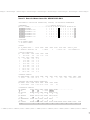
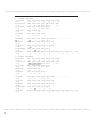
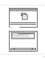
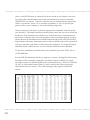
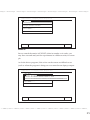
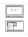
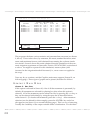
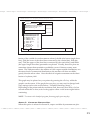
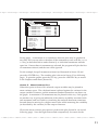
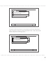
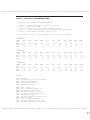
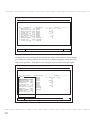
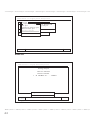
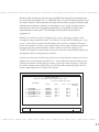
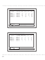
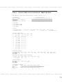
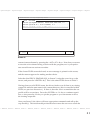
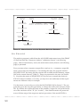
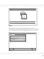
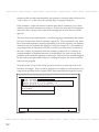
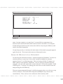
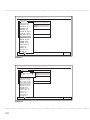
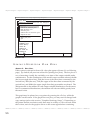
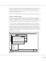
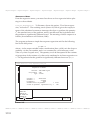
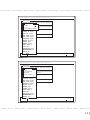
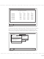
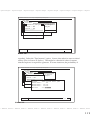
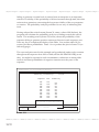
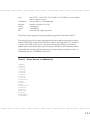
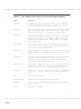
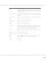
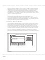
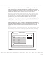
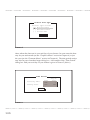
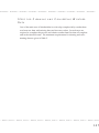
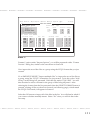
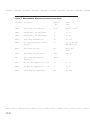
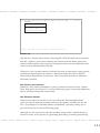
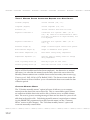
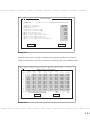
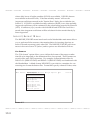
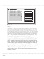
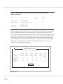
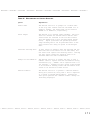
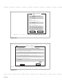
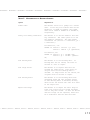
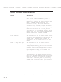
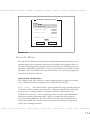
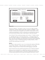
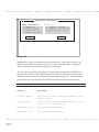
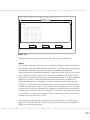
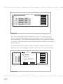
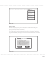
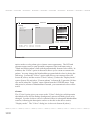
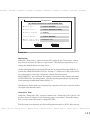
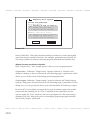
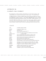
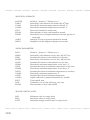
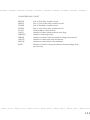
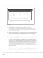
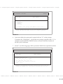
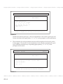
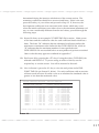
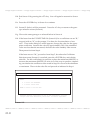
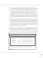
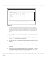
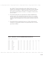
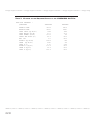
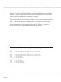
WeatherMan ¥ WeatherMan ¥ WeatherMan ¥ WeatherMan ¥ WeatherMan ¥ WeatherMan ¥ WeatherMan ¥ WeatherMan ¥ WeatherMan ¥ WeatherMa
TABLE 4. WEATHER STATION INFORMATION REQUIRED
FOR A
NEW STATION.
Latitude (degrees)
Station latitude (+=N, -=S).
Longitude (degrees)
Station longitude (+=E, -=W).
Elevation (m)
Station elevation above mean sea level.
Angstrom coefficient A
Coefficient A in equation: SRAD = (A + B *
n/N) * RE, where RE is extraterrestrial radiation and n is duration of bright sunshine, and
N is daylength.
Angstrom coefficient B
Coefficient B in equation: SRAD = (A + B *
n/N) * RE.
Reference height (m)
Height of meteorological sensors above ground.
Wind reference height (m)
Height of anemometer above ground.
Mean annual temperature (°C)
Mean annual average daily temperature.
Temperature amplitude (°C)
Half the range of monthly means for average
daily temperature.
Start of growing season (d)
Mean day-of-year for last frost.
Duration growing season (d)
Mean time from last frost to first frost.
Export will be dis-abled until it has been completed. An alternative to manual
data entry is to calculate the means from the daily data in the raw archive file.
Monthly climate statistics are available from several secondary data sources (eg.
Conway, et al., 1963; NOAA, 1974; Rudloff, 1981). The last two items in the dialog box shown in Screen 16 allow you to document the data source and the data
collection period.
CALCULATE MONTHLY MEANS
The ÒCalculate monthly meansÓ option in Screen 14 allows you to compute
means from the data in the raw archive file. This is a reasonable option if there
are sufficient reliable data in the archive file or if there are no available climate
data. The user is given a warning message if there are less than five years of reliable data in the archive file. Calculating monthly means is equivalent to estimating the SIMMETEO parameters from the Generate menu (see the ÒGenerate
MenuÓ section in this Chapter). The ÒCalculate monthly meansÓ option will
overwrite manually-entered data.
DSSAT v3, Volume 3 ¥ DSSAT v3, Volume 3 ¥ DSSAT v3, Volume 3 ¥ DSSAT v3, Volume 3 ¥ DSSAT v3, Volume 3 ¥ DSSAT v3, Volume 3 ¥ DSSAT v3, V
162
WeatherMan ¥ WeatherMan ¥ WeatherMan ¥ WeatherMan ¥ WeatherMan ¥ WeatherMan ¥ WeatherMan ¥ WeatherMan ¥ WeatherMan ¥ WeatherMan ¥
[ ]
Station Data
Location:
Gainesville,Florida
Latitude (degrees):
Longitute (degrees):
Elevation (m):
Angstrom coefficient A:
Angstrom coefficient B:
Reference height (m):
Wind reference height (m):
Mean annual temperature (°C):
Temperature amplitude (°C):
Start of growing season (day):
Duration of growing season (days):
29.630
-82.370
10.0
0.25
0.50
1.00
3.00
20.9
7.5
1
365
OK
Cancel
SCREEN 15.
Monthly mean hours of bright sunshine and Angstrom coefficients (Prescott,
1940) are included to aid in the estimation of missing daily solar radiation data
File Station Import/Export Generate Analyze Options Quit
12:51:39
[ ]
Monthly Means and Rainfall
Mean
--mean monthly values-Total Number
Angstrom coef.
A
TMAX
B
SPRAD
TMIN
rain of wet
SUNH
(%) (Y-int) (slope)
(°C)
(°C)
Mon (MJ/m2)
(mm)
days
1
19.3
5.7
94.2
-99.0
0.500
8.7
0.250
10.9
2
21.2
118.3
-99.0
7.2
0.500
8.3
0.250
13.4
3
24.3
109.8
-99.0
10.0
0.500
8.3
0.250
17.2
4
28.0
78.7
-99.0
13.5
0.500
5.8
0.250
21.4
5
30.9
101.1
-99.0
17.1
0.500
7.9
0.250
22.3
6
32.5
165.9
-99.0
20.6
0.500
12.4
0.250
20.8
7
33.1
175.1
-99.0
16.5
21.9
0.500
20.3
0.250
32.9
201.9
-99.0
8
16.2
21.9
0.500
18.8
0.250
31.6
136.2
-99.0
11.3
16.6
20.6
0.500
9
0.250
28.6
56.9
-99.0
6.5
14.6
16.3
0.500
0.250
10
24.5
59.3
-99.0
6.0
12.0
11.5
0.500
0.250
11
9.9
21.5
6.8
69.3
-99.0
7.9
0.250
0.500
12
Source:Calculated_from_daily_data
OK
F1 Help
Stn: UFGA
1st year: 1980
No. years: 25
Cancel
| Mean solar radiation (MJ/m2/d) for month.
SCREEN 16.
¥ DSSAT v3, Volume 3 ¥ DSSAT v3, Volume 3 ¥ DSSAT v3, Volume 3 ¥ DSSAT v3, Volume 3 ¥ DSSAT v3, Volume 3 ¥ DSSAT v3, Volume 3 ¥ DSSAT v3, Volume
163
WeatherMan ¥ WeatherMan ¥ WeatherMan ¥ WeatherMan ¥ WeatherMan ¥ WeatherMan ¥ WeatherMan ¥ WeatherMan ¥ WeatherMan ¥ WeatherMa
where daily hours of bright sunshine (SUNH) are available. If SUNH data are
not available in the archive file, ÒCalculate monthly meansÓ will use the
Angstrom coefficients entered in the ÒStation DataÓ dialog box as defaults (see
Screen 15). If SUNH is available but daily radiation (SRAD) is not, then monthly
Angstrom coefficients will be estimated by the relationship proposed by Rietveld
(1978). If sufficient (>5yr) records with both SRAD and SUNH are found for a
month, then Angstrom coefficients will be calculated for that month directly by
linear regression.
IMPORT/EXPORT MENU
The IMPORT/EXPORT menu item found on the WeatherMan main menu allows
you to perform all the necessary data manipulation for inserting data into an
archive file and extracting it into other files. The IMPORT/EXPORT pull-down
menu is shown in Screen 17 (below) and its options are described as follows.
FILE FORMATS
The ÒFile formatÓ option allows you to define the format of the target weather
data file to be imported or the destination file to be exported. These formats are
saved in files with .FMT extensions. For example, format definition files for
DSSAT v2.1 (IBSNAT2.FMT) and DSSAT v3 (IBSNAT3.FMT) are distributed with
the WeatherMan. A blank format, NEW.FMT, is provided as a template for constructing new format definition files. Format files specify columns of data, units
File
Station
Import/Export
Generate
Analyze
Options
Quit
14:08:26
Convert format
Import single file
Import multiple files
Import options
Edit range checks
Export single file
Export yearly files
Export options
Data fill options
SCREEN 17.
DSSAT v3, Volume 3 ¥ DSSAT v3, Volume 3 ¥ DSSAT v3, Volume 3 ¥ DSSAT v3, Volume 3 ¥ DSSAT v3, Volume 3 ¥ DSSAT v3, Volume 3 ¥ DSSAT v3, V
164
WeatherMan ¥ WeatherMan ¥ WeatherMan ¥ WeatherMan ¥ WeatherMan ¥ WeatherMan ¥ WeatherMan ¥ WeatherMan ¥ WeatherMan ¥ WeatherMan ¥
for each data column, date formats (i.e., year/month/day or year/day of year),
and file header options. Users can edit these formats and save the changes under
new or existing names.
The ÒFormat NameÓ dialog box that appears during Import, Export, and Convert
operations is a variation of the ÒFile ListÓ dialog box (see Screen 10) with an additional EDIT button. The EDIT button allows the user to view, edit, and save format files. If a name is entered that doesnÕt match an existing format, the user will
be prompted to edit a blank template format, NEW, and save it under the desired
name. The ÒEdit File FormatÓ dialog box presented when the EDIT button is
pressed is shown in Screen 18 (below).
In Screen 18, the format name is displayed in the top right corner window. The
ÒHeader output optionÓ in the top left region of the screen controls what header
lines are added to a file during an Export operation. The header can match
DSSAT v3 or v2.1 standards, consist of variable names right-justified in the
columns in which the variables will be written, or can be read from a text file.
Just below the ÒHeader output optionÓ is the ÒNo. header lines:Ó which is the
number of non-blank header lines to be skipped during Import.
The format for the date is entered in the upper right hand corner in Screen 18.
For Import, the date of the first data point should be entered only if dates are not
File Station Import/Export Generate Analyze Options Quit
[ ]
Edit File Format
Header output option:
Format name:
IBSNAT3
( ) None
Position
First
Date:
( ) IBSNAT v.3
Year
( ) IBSNAT v.2
1990
1
Month
( ) Variable names
1
0
Day
( ) From header file
1
9
4
No. header lines:
1
2
3
4
5
6
Variable
SRAD ↓
TMAX ↓
TMIN ↓
RAIN ↓
↓
↓
OK
Units
MJ/m2
°C
°C
mm
↓
↓
↓
↓
↓
↓
Pos. Len.
5
7
5
13
5
19
5
25
0
0
0
0
Cancel
7
8
9
10
11
12
Variable
↓
↓
↓
↓
↓
↓
View file
Units
↓
↓
↓
↓
↓
↓
14:39:35
Length
2
0
3
Pos.
0
0
0
0
0
0
Len.
0
0
0
0
0
0
Save format
SCREEN 18.
¥ DSSAT v3, Volume 3 ¥ DSSAT v3, Volume 3 ¥ DSSAT v3, Volume 3 ¥ DSSAT v3, Volume 3 ¥ DSSAT v3, Volume 3 ¥ DSSAT v3, Volume 3 ¥ DSSAT v3, Volume
165
WeatherMan ¥ WeatherMan ¥ WeatherMan ¥ WeatherMan ¥ WeatherMan ¥ WeatherMan ¥ WeatherMan ¥ WeatherMan ¥ WeatherMan ¥ WeatherMa
explicitly given in the import file. The date format can be year, month and day-ofmonth or year and day-of-year. The day-of-year format is inferred from a length of
0 for month and a length ³3 for the day.
Up to 12 variables can be imported in any order and with any units. The variables
and their units are entered in the lower left-hand windows in Screen 18. The choice
of variables and their units is made with lists that are activated by the down arrow
or double clicking with the left mouse button on the appropriate cell in these windows. Moving from cell-to-cell is achieved with the <TAB> and <SHIFT>-<TAB>
keys or single-clicking with the left mouse button. Based on the chosen variable,
the list will reflect valid units. For example, for temperature variables only temperature units are listed (¡C, ¡F, ¡K). The variables in the list and their associated units
and conversion factors are contained in an external file (WM.VAR). Please contact
the authors if you want to modify the list of variables.
The VIEW FILE button provides a file viewer to facilitate the choice of the position
and length of the variables in the data file (see Screen 19, below).
The SAVE FORMAT button provides access to a ÒFile ListÓ dialog box so that a
new or modified format can be saved to a file for subsequent use. The OK button
will accept any format changes for the current IMPORT/EXPORT session but will
not save them to a file, so when you quit the operation, any changes you have made
to the format will be lost.
File
Station
Import/Export
Generate Analyze
Edit File Format
Header output option:
( ) None
( ) IBSNAT v.3
( ) IBSNAT v.2
( ) Variable names
( ) From header file
No. header lines:
4
1
2
3
4
5
6
Variable
SRAD ↓
TMAX ↓
TMIN ↓
RAIN ↓
↓
↓
Units
MJ/m2
°C
°C
mm
[ ]
2
1
Format name:
Date:
Year
Month
Day
↓
↓
↓
↓
↓
↓
Pos.
7
13
19
25
0
0
Len.
5
5
5
5
0
0
Options
09:42:09
IBSNAT3
First
1900
1
1
Position
1
0
3
Variable
7
8
9
10
11
12
Quit
Units
↓
↓
↓
↓
↓
↓
↓
↓
↓
↓
↓
↓
C:\DSSAT3\WEATHER\UFGA8001.WTH
5
4
3
Length
2
0
3
Pos.
0
0
0
0
0
0
Len.
0
0
0
0
0
0
[↑ ]
6
7
*WEATHER : GAINESVILLE,FLORIDA,USA
@ INSI
UFGA
F1 Help
LAT
29.630
F10 Menu
LONG
-82.370
ELEV
10
TAV
20.9
AMP REFHT WNDHT
7.5 2.00 3.00
Stn: UFGA
SCREEN 19.
DSSAT v3, Volume 3 ¥ DSSAT v3, Volume 3 ¥ DSSAT v3, Volume 3 ¥ DSSAT v3, Volume 3 ¥ DSSAT v3, Volume 3 ¥ DSSAT v3, Volume 3 ¥ DSSAT v3, V
166
WeatherMan ¥ WeatherMan ¥ WeatherMan ¥ WeatherMan ¥ WeatherMan ¥ WeatherMan ¥ WeatherMan ¥ WeatherMan ¥ WeatherMan ¥ WeatherMan ¥
The VIEW FILE button displays the file in conjunction with a ruler as shown in
Screen 19.
If a format is being edited during an Import operation and the ÒPreview formatsÓ
option is enabled (with a tick mark) in the ÒImport OptionsÓ dialog box (see Screen
24), then a ÒPreview FormatÓ dialog box (Screen 20, below) will be presented when
either the OK or the SAVE button is pressed. The ÒPreview FormatÓ dialog box
displays a file viewer which shows the first 50 records of the weather file. The
columns where the program, using the current format, will look for variables are
labeled and highlighted.
CONVERT FORMAT
The ÒConvert formatÓ option found in the IMPORT/EXPORT pull-down menu
(see Screen 17) allows you to convert a weather data file from one format and set of
units to another without defining a weather station. A permanent archive file for
the raw data is not retained, and range checking and data fill are not performed.
When converting a weather file format, the user will be prompted to: (1) select the
target file to convert from, (2) select a format name for the target file, (3) select the
destination file name to convert to, and (4) select a format for the destination file.
The file names and format names are selected using the ÒFile ListÓ dialog box (see
Screen 10 or Screen 21, on following page).
[ ]
Preview Format
The highlighted text shows how WeatherMan will parse the first 50
records in UFGA8001.WTH based on the current format.
Continue?
C:\DSSAT3\WEATHER\UFGA8001.WTH
Yr Dy
80001
80002
80003
80004
80005
80006
80007
80008
80009
SRAD
8.7
13.9
13.0
2.0
13.6
14.2
13.6
9.1
6.8
TMAX
14.4
17.2
18.9
18.9
16.1
12.2
20.0
22.8
23.9
Yes
TMIN
2.8
-1.1
-1.1
5.0
5.0
-2.2
-1.1
5.0
10.6
RAIN
0.0
0.0
0.0
27.9
0.0
0.0
0.0
0.0
0.0
18.5
28.7
27.6
5.4
27.8
28.9
7.3
20.1
15.6
No
SCREEN 20.
¥ DSSAT v3, Volume 3 ¥ DSSAT v3, Volume 3 ¥ DSSAT v3, Volume 3 ¥ DSSAT v3, Volume 3 ¥ DSSAT v3, Volume 3 ¥ DSSAT v3, Volume 3 ¥ DSSAT v3, Volume
167
WeatherMan ¥ WeatherMan ¥ WeatherMan ¥ WeatherMan ¥ WeatherMan ¥ WeatherMan ¥ WeatherMan ¥ WeatherMan ¥ WeatherMan ¥ WeatherMa
[ ]
Files To Import
Weather file
UFGA7601.WTH
UFGA7801.WTH
UFGA7901.WTH
UFGA8101.WTH
UFGA8201.WTH
UFGA8401.WTH
UFGA8601.WTH
UFGA8001.WTH
Format
IBSNAT3
IBSNAT3
IBSNAT3
IBSNAT3
IBSNAT3
IBSNAT3
IBSNAT3
IBSNAT3
Add file
Remove file
Select format
Add Group
Cancel
OK
SCREEN 21.
IMPORT...
The ÒImport...Ò option can be used to import a single file or a set of files into an
archive file. The ÒImport single fileÓ option uses the standard ÒFile ListÓ dialog
box to select a import file name and format. These steps are identical to the first
two steps discussed in the above ÒConvert formatÓ section. The ÒImport multiple
filesÓ option builds a list of files and their corresponding formats. This feature is
useful where the weather variables are stored in different files with different formats, or for a group of files with the same format. The ÒFiles To ImportÓ dialog
box presented when this option is selected is shown in Screen 21.
In Screen 21, the ADD FILE button activates the IMPORT/EXPORT ÒFile NameÓ
dialog box and adds a file to the list displayed in the left-hand window of this
screen. The REMOVE FILE button can be used to delete a highlighted file from
the list. The first file chosen is inserted into the list with a format of Ònone.Ó The
SELECT FORMAT button activates the ÒFormat NameÓ dialog box and the user
can access the ÒEdit File FormatÓ dialog box using the EDIT button in that dialog
box. Adding subsequent files automatically assigns them the format name of the
highlighted line. This feature facilitates adding several files with the same format
to the list. The format of a highlighted file may also be modified from the
SELECT FORMAT button. Files in the list are imported sequentially when the
OK button is selected.
DSSAT v3, Volume 3 ¥ DSSAT v3, Volume 3 ¥ DSSAT v3, Volume 3 ¥ DSSAT v3, Volume 3 ¥ DSSAT v3, Volume 3 ¥ DSSAT v3, Volume 3 ¥ DSSAT v3, V
168
WeatherMan ¥ WeatherMan ¥ WeatherMan ¥ WeatherMan ¥ WeatherMan ¥ WeatherMan ¥ WeatherMan ¥ WeatherMan ¥ WeatherMan ¥ WeatherMan ¥
[ ]
Import Group File Mask
Path and file mask:
ufga*.wth
OK
↓
Cancel
SCREEN 22.
A group of files with similar names can also be added using the ADD GROUP button in Screen 21. This feature is especially useful for importing many one-year file
of the same format. Since a file mask is used to define the group, unwanted file
names are occasionally inserted in the list, but these are easily removed by use of
the REMOVE FILE button. The ÒImport Group File MaskÓ dialog box used to
define the group is shown in Screen 22 (above).
If the ÒPreview formats optionÓ is enabled under the ÒImport OptionsÓ dialog box
(Screen 24), a ÒPreview FormatÓ dialog box (Screen 20) will be presented before
each file is imported.
OnÓImport,Ó variables that have errors or are suspect are automatically flagged
(see the section ÒImport OptionsÓ in this Chapter and Screen 23 to change this setting). The flags used are lower case letters. When an original value is filled-in, its
flag is converted to upper case. The flags and their meaning are listed in Table 5.
At the end of the ÒImportÓ process, a summary report is given indicating the
quantity and quality of data in the raw archive file. An example of this report is
displayed in the ÒImport StatisticsÓ dialog box as shown in Screen 23 (on following
page).
IMPORT OPTIONS
The options for import can be changed using the ÒImport optionsÓ menu item
from Screen 17 which accesses the ÒImport OptionsÓ dialog box presented in
Screen 24 and explained in Table 6.
¥ DSSAT v3, Volume 3 ¥ DSSAT v3, Volume 3 ¥ DSSAT v3, Volume 3 ¥ DSSAT v3, Volume 3 ¥ DSSAT v3, Volume 3 ¥ DSSAT v3, Volume 3 ¥ DSSAT v3, Volume
169
WeatherMan ¥ WeatherMan ¥ WeatherMan ¥ WeatherMan ¥ WeatherMan ¥ WeatherMan ¥ WeatherMan ¥ WeatherMan ¥ WeatherMan ¥ WeatherMa
TABLE 5. EXPLANATION
ERRONEOUS DATA.
OF
ERROR CODES USED
Class
Description
Range check
Range check
Range check
Above maximum
Below minimum
Greater than maximum
daily change
Missing value
Format error
Conversion
Conversion
TO
FLAG SUSPECT
Import
code
Filled
code
a
b
A
B
r
n
e
R
N
E
OR
When range checking is turned on, the variables are checked against a maximum
value, a minimum value, and a maximum rate of change from one day to the
next. The values inserted in the raw archive file are not changed but marked with
an appropriate range check flag (see the ÒImportÓ section above). Default range
values are provided for a new weather station and these can be edited using the
ÒEdit range checksÓ option found in Screen 17 to access the ÒEdit Check RangesÓ
dialog box. An example of the ÒEdit Check RangesÓ dialog box is shown in
Screen 25 (on second following page).
[ ]
Import Statistics
Records in UFGA.WTD
TOTAL :
VALID :
MISSING:
ERROR :
ABOVE :
BELOW :
RATE
:
TOTAL
43380
43089
277
0
1
12
1
SRAD
8676
8670
0
0
0
6
0
TMAX
8676
8673
0
0
0
3
0
TMIN
8676
8675
0
0
0
0
1
RAIN
8676
8676
0
0
0
0
0
PAR
8676
8395
277
0
1
3
0
OK
SCREEN 23.
DSSAT v3, Volume 3 ¥ DSSAT v3, Volume 3 ¥ DSSAT v3, Volume 3 ¥ DSSAT v3, Volume 3 ¥ DSSAT v3, Volume 3 ¥ DSSAT v3, Volume 3 ¥ DSSAT v3, V
170
WeatherMan ¥ WeatherMan ¥ WeatherMan ¥ WeatherMan ¥ WeatherMan ¥ WeatherMan ¥ WeatherMan ¥ WeatherMan ¥ WeatherMan ¥ WeatherMan ¥
TABLE 6. EXPLANATION
OF
IMPORT OPTIONS.
Option
Explanation
Format name:
The default action is to prompt for a format name.
If the only file formats used are the DSSAT v2.1 or
DSSAT v3 formats, the format name can be fixed as
IBSNAT v2 or IBSNAT v3, respectively.
Check ranges:
The default is to perform range checking. The variables are checked for extreme values and the unaltered values are inserted in the raw data archive
file and marked with a flag (see Edit Range Checks
below). Import operations can speeded up without
range checking and it can be performed later on the
whole archive file using an option in the Analyze
menu.
Overwrite existing data:
If this option is enabled, when the existing and new
data both have valid values for the same dates, the
new values will replace the existing values. Turning
off this option causes the existing value to be
retained under the same circumstances.
Prompt for non-numerics:
The default action is to prompt the user to give a
numeric value to replace each new non-numeric string
encountered (e.g., “TRACE” can be replaced with ‘0.0’
for rainfall.) Turning off this option causes blanks
to be treated as missing values and non-numeric characters to be treated as format errors.
Preview formats:
The default action is to present a “Preview Format”
dialog box (Screen 20) every time a file is imported
or a format is edited during Import. Turning-off
this option prevents the “Preview Format” dialog box
from being displayed.
¥ DSSAT v3, Volume 3 ¥ DSSAT v3, Volume 3 ¥ DSSAT v3, Volume 3 ¥ DSSAT v3, Volume 3 ¥ DSSAT v3, Volume 3 ¥ DSSAT v3, Volume 3 ¥ DSSAT v3, Volume
171
WeatherMan ¥ WeatherMan ¥ WeatherMan ¥ WeatherMan ¥ WeatherMan ¥ WeatherMan ¥ WeatherMan ¥ WeatherMan ¥ WeatherMan ¥ WeatherMa
[ ]
Import Options
Format name:
( ) Prompt for name.
( ) IBSNAT3
( ) IBSNAT2
Other options:
[X] Check ranges.
[X] Overwrite existing data.
[X] Prompt for non-numerics.
[X] Preview formats
OK
Cancel
SCREEN 24.
All variables in Screen 25 are in the archive file units except for solar radiation
(SRAD) and photosynthetically active radiation (PAR) which are in percent of
extraterrestrial radiation. Updated ranges are saved to the weather station climate file. The DEFAULTS button restores the default values.
[ ]
Edit Check Ranges
Variable Minimum
SRAD*
5.0
TMAX
5.0
TMIN
-20.0
0.0
RAIN
0.0
DEWP
0.0
WIND
0.0
SUNH
5.0
PAR *
0.0
TDRY
0.0
TWET
0.0
EVAP
Maximum
85.0
40.0
30.0
600.0
25.0
500.0
100.0
85.0
35.0
25.0
15.0
MaxRate
70.0
20.0
20.0
500.0
5.0
300.0
90.0
70.0
20.0
20.0
15.0
*Radiation in % of extraterrestrial.
OK
SCREEN 25.
172
Defaults
Cancel
WeatherMan ¥ WeatherMan ¥ WeatherMan ¥ WeatherMan ¥ WeatherMan ¥ WeatherMan ¥ WeatherMan ¥ WeatherMan ¥ WeatherMan ¥ WeatherMan ¥
EXPORT...
The ÒExport...Ó option in Screen 17 can be used to export a single file or a set of
yearly files. The ÒExport single fileÓ option uses the ÒArchive TypeÓ dialog box
(Screen 4) (if the raw archive file is not the only type), ÒTime PeriodÓ dialog box
(Screen 5), and the ÒFile ListÓ dialog box (Screen 2) to select an export file name
and format. The ÒExport yearly fileÓ option uses the same dialog boxes, but the
file export names are built automatically based on the DSSAT v2.1 or DSSAT v3
file naming conventions. The files can easily be renamed using the DOS
RENAME command. Access to the ÒEdit FormatÓ dialog box is from the
ÒFormat FileÓ dialog box.
During ÒImport,Ó errors or suspect values in the raw archive file are marked
with a flag indicating the source of the error. On ÒExport,Ó if a data item is filled
in, the valueÕs error flag is converted to an upper case letter. This reminds the
user that the value was filled-in and the cause of the error. Error flag definitions
are listed in Table 5.
EXPORT OPTIONS
The options for export can be changed using theÓExport optionsÓ menu item
which accesses the ÒExport OptionsÓ dialog box presented in Screen 26 (on following page) and discussed in Table 7.
When any of the data fill options are turned on in Screen 26 by placing an ÔxÕ in
the left-hand box in the ÒOther options:Ó menu list, there are a number of ways
in which the data fill can be implemented. These options are accessed from the
ÒData fillÓ options menu item that invokes theÓ Data Fill OptionsÓ dialog box
given in Screen 27 (on following page) and discussed in Table 8.
G E N E R AT E M E N U
The GENERATE menu item found on the WeatherMan main menu allows estimation of the weather generator parameters and subsequent generation of daily
weather data. The weather generators used are adaptations of WGEN
(Richardson and Wright, 1984) and SIMMETEO (Geng et al. 1986; Geng and
Auburn, 1988). The SIMMETEO generator is embodied in the WGEN generator
but uses a different input section. The resulting WGEN/SIMMETEO is a translation of the FORTRAN version used internally in the DSSAT v3 crop models. In
this version of WeatherMan, both generators are restricted to generating the
DSSAT v2.1 extended weather data set of solar radiation, maximum temperature,
minimum temperature, rainfall, and PAR.
¥ DSSAT v3, Volume 3 ¥ DSSAT v3, Volume 3 ¥ DSSAT v3, Volume 3 ¥ DSSAT v3, Volume 3 ¥ DSSAT v3, Volume 3 ¥ DSSAT v3, Volume 3 ¥ DSSAT v3, Volume
173
WeatherMan ¥ WeatherMan ¥ WeatherMan ¥ WeatherMan ¥ WeatherMan ¥ WeatherMan ¥ WeatherMan ¥ WeatherMan ¥ WeatherMan ¥ WeatherMa
[ ]
Export Options
Format name:
( ) Prompt for name.
( ) IBSNAT3
( ) IBSNAT2
Yearly file
naming conventions:
( ) IBSNAT v.3
( ) IBSNAT v.2
Other options:
[X] Fill missing data.
[X] Fill range errors.
[ ] Fill missing dates.
[ ] Export data flags.
OK
F1 Help
Cancel
Stn: UFGA | Prompt for a format name on export.
SCREEN 26.
File
Station
[ ]
Import/Export
Generate Analyze
Data Fill Options
Options
Quit
14:19:23
Data fill method:
( ) Generate missing data with WGEN or SIMMETEO.
( ) Monthly means and stochastic rainfall generations.
Solar radiation (SRAD and PAR):
( ) Use method selected above to estimate radiation.
( ) Estimate radiation from sunshine hours.
Short (≤ 7 day) data gaps:
( ) Use method selected above to fill data.
( ) Estimate missing data using 10-day running mean.
Model for weather generation:
( ) WGEN
( ) SIMMETEO
Random seed for generator (1 to 32767):
OK
F1 Help
3823
Cancel
Stn: UFGA | Use a stochastic generator to fill missing data.
SCREEN 27.
DSSAT v3, Volume 3 ¥ DSSAT v3, Volume 3 ¥ DSSAT v3, Volume 3 ¥ DSSAT v3, Volume 3 ¥ DSSAT v3, Volume 3 ¥ DSSAT v3, Volume 3 ¥ DSSAT v3, V
174
WeatherMan ¥ WeatherMan ¥ WeatherMan ¥ WeatherMan ¥ WeatherMan ¥ WeatherMan ¥ WeatherMan ¥ WeatherMan ¥ WeatherMan ¥ WeatherMan ¥
TABLE 7. EXPLANATION
OF
EXPORT OPTIONS.
Option
Explanation
Format name:
The default action is to prompt for a format
name. If the only file formats used are the
DSSAT v2.1 or DSSAT v3 formats, the format
name can be fixed as IBSNAT v2 or IBSNAT v3,
respectively.
Yearly file naming convention:
The default is to use the DSSAT v3 file naming convention. The other option is to use
the DSSAT v2 convention. The file naming
conventions are (Station = 4 characters, yr =
2 characters):
For DSSAT v2.1, use
IBSNAT v2: Station + ‘0112.W’ + yr (raw)
Station + ‘GEN.W’ + yr (generated)
For DSSAT v3, use
IBSNAT v3: Station + yr + ‘01.WTH’(raw)
Station + yr + ‘01.WTG’ (generated)
Fill missing data:
The default is to fill missing data. If
missing data are not filled, the value is
written as -99.0 on output.
Fill range errors:
The default is to replace data that are
flagged for range errors. This option is
only in effect if Fill Missing Data is
checked. If range errors are not filled, the
original value is written on output.
Fill missing dates:
The default is to fill missing dates with
sequential dates and fill variable values.
If Fill Missing Dates is disabled, missing
dates in the raw archive file will also exist
in the output file.
Export Data Flags:
The default is to export the error flags as
lower case if data are not filled and upper
case if they were filled. If data are filled
and error flags are not exported, there will
be no indication that the data have been
¥ DSSAT v3, Volume 3 ¥ DSSAT v3, Volume 3 ¥ DSSAT v3, Volume 3 ¥ DSSAT v3, Volume 3 ¥ DSSAT v3, Volume 3 ¥ DSSAT v3, Volume 3 ¥ DSSAT v3, Volume
175
WeatherMan ¥ WeatherMan ¥ WeatherMan ¥ WeatherMan ¥ WeatherMan ¥ WeatherMan ¥ WeatherMan ¥ WeatherMan ¥ WeatherMan ¥ WeatherMa
TABLE 8. EXPLANATION
OF
DATA FILL OPTIONS.
Option
Explanation
Data fill method:
There are two generic data fill methods for all
data. Solar radiation and short periods of
missing data have additional methods. The first
method is to generate all missing data with the
WGEN or SIMMETEO weather generators (see
Generator section). The second method uses
monthly means from the climate file for all
variables except rainfall; a simple stochastic
generator is used for rainfall. Using monthly
means for rainfall is not an option since it
would cause severe problems with any water balance model if all days had some rainfall. Both
methods only fill solar radiation, maximum and
minimum temperature, rainfall, and PAR.
Solar radiation:
The default is to use the generic method selected above. An alternative is to estimate solar
radiation using the Angstrom coefficients in the
climate file. Sunshine hours data must be
available in the raw archive file to use this
method.
Short (≤ 7 Day) data gaps:
The default is to use the generic data fill
method given above. An alternative is to use a
10-day running mean for gaps that are less than
7 days long. This may give a more realistic
estimate of the actual average values for that
period than using long-term means. For data
gaps longer than 7 days, the above data fill
methods will still be used.
Model for weather generation:
The default is to use the SIMMETEO model since
it requires only the monthly means in the climate file. The WGEN model provides better estimates of variability if it has been parameterized from at least five years of good quality
daily data. Model parameters must be in the
climate file to use this option (see Generator
section).
DSSAT v3, Volume 3 ¥ DSSAT v3, Volume 3 ¥ DSSAT v3, Volume 3 ¥ DSSAT v3, Volume 3 ¥ DSSAT v3, Volume 3 ¥ DSSAT v3, Volume 3 ¥ DSSAT v3, V
176
WeatherMan ¥ WeatherMan ¥ WeatherMan ¥ WeatherMan ¥ WeatherMan ¥ WeatherMan ¥ WeatherMan ¥ WeatherMan ¥ WeatherMan ¥ WeatherMan ¥
The DSSAT v3 modifications of WGEN/SIMMETEO use standard deviations
rather than coefficients of variation which makes the generators more stable than
the original versions. Monthly input parameters are now used for all variables,
with linear interpolation computed internally. The modified SIMMETEO model
uses monthly climate parameters and regression equations (Geng, et al. 1988;
Geng and Auburn, 1986; Pickering et al. 1988) to compute the standard deviations.
The GENERATE menu provides the utilities necessary for estimating the generator parameters and generating daily data. The GENERATE menu is shown in
Screen 28 (below) and its options are described as follows.
CALCULATE PARAMETERS
When the ÒCalculate parametersÓ option shown in Screen 28 is selected, the
ÒCalculate ParametersÓ dialog box, shown in Screen 29 (on following page), is
presented.
From Screen 29, the parameters for WGEN or SIMMETEO can be computed separately or together. A standard ÒTime PeriodÓ dialog box (i.e., ÒStartingÓ and
ÒEndingÓ dates) is included in the dialog box shown in Screen 29, allowing you to
choose a particular time period if desired. The default is to use all the data in the
archive file, and the dates presented when Screen 29 appears should represent the
range of dates available in the archive file. The computed monthly parameters
are recorded in the climate file. Estimating the SIMMETEO parameters is equivalent to calculating monthly means from the STATION menu (see Screen 14)Ñboth
File
Station
Import/Export
Generate
Analyze
Options
Quit
14:55:44
Calculate parameters
Generate data
SCREEN 28.
¥ DSSAT v3, Volume 3 ¥ DSSAT v3, Volume 3 ¥ DSSAT v3, Volume 3 ¥ DSSAT v3, Volume 3 ¥ DSSAT v3, Volume 3 ¥ DSSAT v3, Volume 3 ¥ DSSAT v3, Volume
177
WeatherMan ¥ WeatherMan ¥ WeatherMan ¥ WeatherMan ¥ WeatherMan ¥ WeatherMan ¥ WeatherMan ¥ WeatherMan ¥ WeatherMan ¥ WeatherMa
[ ]
Calculate Parameters
Model:
( ) WGEN generator parameter
( ) SIMMETEO monthly means
( ) Both sets of parameters
Starting date:
Year
1980
Ending date:
1987
OK
Day of
year
1
365
Cancel
SCREEN 29.
calculate the same statistics. If the monthly means in the climate file are from a
longer and more reliable record than the daily data, the user should not estimate
SIMMETEOÕs parameters since the monthly means in the climate file will be overwritten. Estimating generator parameters is a reasonable option if there are sufficient reliable data in the raw archive file or if there are no available climate data.
The user is warned if there are less than five years of reliable data in the archive file.
GENERATE DATA
The ÒGenerate dataÓ menu item accesses the ÒGenerate Weather DataÓ dialog box
which is shown in Screen 30 (on following page).
Generated data are output to an archive file called Station_GEN.WTD. This file is
usually treated as a temporary file for the duration of the WeatherMan session (see
the following section entitled, ÒOptions MenuÓ and the subsection ÒTemporary
FilesÓ for a description of how to change from a temporary file). Either the WGEN
or SIMMETEO generator can be used to generate daily data. The standard ÒTime
PeriodÓ dialog box is inserted to choose the years to be generated; only full years can
be generated. The default action is to match the time period of the raw archive file,
although any time period can be specified. For comparing yearly time series graphically, matching the dates is a good choice. Just because generated and raw data have
the same time period does not mean that the generated data predict the raw daily
data; only the means are predicted on average. A random number seed is generated
and inserted in the dialog box shown in Screen 30. To generate an identical sequence
of weather data, the same random number seed should be specified.
DSSAT v3, Volume 3 ¥ DSSAT v3, Volume 3 ¥ DSSAT v3, Volume 3 ¥ DSSAT v3, Volume 3 ¥ DSSAT v3, Volume 3 ¥ DSSAT v3, Volume 3 ¥ DSSAT v3, V
178
WeatherMan ¥ WeatherMan ¥ WeatherMan ¥ WeatherMan ¥ WeatherMan ¥ WeatherMan ¥ WeatherMan ¥ WeatherMan ¥ WeatherMan ¥ WeatherMan ¥
[ ]
Generate Weather Data
Model:
( ) WGEN
( ) SIMMETEO
Starting year:
1980
Ending year:
1987
Random seed (1 to 32767):
3919
OK
Cancel
SCREEN 30.
A N A LY Z E M E N U
The ANALYZE menu item found on the WeatherMan main menu allows you to
calculate and present summary statistics in both tabular and graphical form. It
also repeats the range check and data fill functions that are normally done automatically on IMPORT or EXPORT. Analysis is performed on raw, filled or generated data. The ANALYZE menu is shown in Screen 31 (on following page) and
its options described as follows.
RANGE CHECK
AND
DATA FILL
The ÒRange checkÓ and ÒData fillÓ options listed in Screen 31 offer you another
way to perform functions normally done on IMPORT or EXPORT.
Range check. The ÒRange checkÓ option permits the range checking analysis
to be done on the complete raw archive file. After the check is done, the results
are given in an ÒImport StatisticsÓ dialog box similar to the dialog box for
IMPORT (see Screen 23). This re-checking process is useful when IMPORT has
been done with incorrect range check values or if range checking had been
turned off during IMPORT. It is also useful for identifying a reasonable set of
range check values for a weather station by iteratively setting the range check
values and viewing the results.
¥ DSSAT v3, Volume 3 ¥ DSSAT v3, Volume 3 ¥ DSSAT v3, Volume 3 ¥ DSSAT v3, Volume 3 ¥ DSSAT v3, Volume 3 ¥ DSSAT v3, Volume 3 ¥ DSSAT v3, Volume
179
WeatherMan ¥ WeatherMan ¥ WeatherMan ¥ WeatherMan ¥ WeatherMan ¥ WeatherMan ¥ WeatherMan ¥ WeatherMan ¥ WeatherMan ¥ WeatherMa
File
Station
Import/Export
Generate
Analyze
Options
Quit
14:55:44
Range check
Data fill
Statistics
Report
Graph
SCREEN 31.
Data fill. The ÒData fillÓ option creates a filled archive file called
Station_FIL.WTD. This file is usually treated as a temporary file for the duration
of the WeatherMan session (see the following section entitled, ÒOptions MenuÓ
and the subsection ÒTemporary FilesÓ for a description of how to change from a
temporary file). The filled archive file can be analyzed and compared with the
raw data to check the data fill algorithms.
STATISTICS
The ÒStatisticsÓ menu item listed in Screen 31 provides algorithms for summarizing the data in various ways. When this option is selected, the ÒArchive TypeÓ
dialog box is presented (Screen 32, on following page). This dialog box allows
you to choose raw, filled, or generated archive files.
Statistics are output to summary files and are usually treated as temporary files
for the duration of the WeatherMan session ( see the following section entitled,
ÒOptions MenuÓ and the subsection ÒTemporary FilesÓ for a description of how
to change from a temporary file). The SUM files are also used for the ÒReportÓ
and ÒGraphÓ options under the ANALYZE menu. The ÒTime PeriodÓ dialog box
allows the user to choose the time period to be analyzed. The default action is to
analyze the whole archive file.
In Screen 32, there are four types of statistics to select from: ÒMoments,Ó
ÒPercentiles,Ó ÒDistributionÓ and ÒTime structure.Ó The default choice is to calculate moments only. ÒMomentsÓ includes means, standard deviations, and
DSSAT v3, Volume 3 ¥ DSSAT v3, Volume 3 ¥ DSSAT v3, Volume 3 ¥ DSSAT v3, Volume 3 ¥ DSSAT v3, Volume 3 ¥ DSSAT v3, Volume 3 ¥ DSSAT v3, V
180
WeatherMan ¥ WeatherMan ¥ WeatherMan ¥ WeatherMan ¥ WeatherMan ¥ WeatherMan ¥ WeatherMan ¥ WeatherMan ¥ WeatherMan ¥ WeatherMan ¥
[ ]
Type
[X]
[ ]
[ ]
[ ]
Summary Statistics
of Statistic:
Momments
Percentiles
Distibution
Time structure
Grouping:
[X] Monthly summary
[ ] Monthly time series
[ ] Yearly time series
Starting date:
Year
1980
Ending date:
1987
OK
Day of year
1
365
Cancel
SCREEN 32.
skewness coefficient. ÒPercentilesÓ are the 0, 25, 50, 75, and 100 percentiles.
ÒDistributionÓ includes both histograms and cumulative probabilities. ÒTime
structureÓ includes autocorrelograms for all variables except rainfall, and has
conditional probabilities for rainfall. All statistics are automatically computed
for wet, dry and for all days, except ÒTime structureÓ which uses all days.
Also in Screen 32, three statistics groupings can be selected: ÒMonthly summary,Ó ÒMonthly time seriesÓ and ÒYearly time series.Ó A fourth grouping comprised of all data combined, is automatically performed with the monthly summary. The time series analyses are relatively slow since they require considerable
sorting prior to output. The default grouping is monthly summary. Table 9
describes these groupings in more detail.
REPORT
The ÒReportÓ option provides a way to view and print the summary (SUM) files
created under ÒStatistics.Ó When this option is selected, the ÒView/Print
StatisticsÓ dialog box shown in Screen 33 (on following page) is presented.
Screen 33 has the same Type and Grouping choices as the ÒSummary StatisticsÓ
dialog box shown in Screen 32. As a default, the same boxes are checked in
Screen 33 as were checked in Screen 32 since those summary files already exist.
If all the selected options have been previously analyzed, the files are viewed
¥ DSSAT v3, Volume 3 ¥ DSSAT v3, Volume 3 ¥ DSSAT v3, Volume 3 ¥ DSSAT v3, Volume 3 ¥ DSSAT v3, Volume 3 ¥ DSSAT v3, Volume 3 ¥ DSSAT v3, Volume
181
WeatherMan ¥ WeatherMan ¥ WeatherMan ¥ WeatherMan ¥ WeatherMan ¥ WeatherMan ¥ WeatherMan ¥ WeatherMan ¥ WeatherMan ¥ WeatherMa
[ ]
Type
[X]
[ ]
[ ]
[ ]
View/Print Statistics
of Statistic:
Momments
Percentiles
Distibution
Time structure
Grouping:
[X] Monthly summary
[ ] Monthly time series
[ ] Yearly time series
Cancel
OK
SCREEN 33.
sequentially. Up to 12 summary files are possible for each type of archive file.
When the OK button is pressed in Screen 33, the ÒSummary FileÓ dialog box
shown in Screen 34 (on following page) is presented.
The user can scroll both vertically and horizontally through the SUM file displayed in Screen 34. If the PRINT button in Screen 34 is pressed, the SUM file
displayed in the window is printed to the parallel printer port. The OK button
displays the next file while the CANCEL button aborts the viewing process.
TABLE 9. EXPLANATION
OF
STATISTICS TIME GROUPINGS.
Grouping
Explanation
All data combined
Pools all data together (computed automatically with
monthly summary).
Monthly summary
Pools all the data from each month together (eg. all of
January’s, all of February’s etc).
Monthly time series
Each month analyzed separately.
Yearly time series
Each year analyzed separately.
DSSAT v3, Volume 3 ¥ DSSAT v3, Volume 3 ¥ DSSAT v3, Volume 3 ¥ DSSAT v3, Volume 3 ¥ DSSAT v3, Volume 3 ¥ DSSAT v3, Volume 3 ¥ DSSAT v3, V
182
WeatherMan ¥ WeatherMan ¥ WeatherMan ¥ WeatherMan ¥ WeatherMan ¥ WeatherMan ¥ WeatherMan ¥ WeatherMan ¥ WeatherMan ¥ WeatherMan ¥
File
[ ]
Station
Import/Export
Generate
Analyze
Options
Quit
Summary File
UFGA_AMA.SUM
! Monthly summary moments for station UFGA observed data.
*SRADDRY
@
MTH
1
2
3
4
5
6
7
8
9
10
SDMN
11.9
14.8
18.8
22.7
23.4
22.4
22.0
20.3
17.7
15.4
SDSD
2.9
3.7
4.1
3.8
3.8
3.6
3.4
2.9
3.3
3.4
OK
F1 Help
SDSK
-0.9
-0.9
-0.8
-1.1
-1.1
-0.8
-0.9
-0.8
-1.0
-0.9
SDKT
0.3
0.3
0.0
1.6
1.2
0.3
1.0
0.6
0.8
0.7
Print
Cancel
Stn: UFGA | Use cursor keys or mouse to scroll, <Esc> or icon to quit.
SCREEN 34.
Variable names that appear in summary files are given in Appendix A.
GRAPH
The ÒGraphÓ option provides access to a graphics package to plot both the data
in the archive files and in the statistics (SUM) files. The following six graph types
are available: Time Plot, Box Plot, Histogram, Cumulative Distribution,
Autocorrelation, and Rainfall Probability. Within each graph type, up to six plots
can be defined (except for the Box Plot and Auto correlation which allow only a
single plot), but only the checked plots will actually be plotted. A plot definition
dialog box is used to create combinations of weather stations, variables, wet
states, and time ranges. A default set of plots is automatically loaded into this
dialog box. The down arrow or mouse can be used to access lists for the Station,
Variable and Wet state columns. Only valid choices are displayed. For example,
if statistics have not been calculated for a particular weather station, the statistics
variables for that station will not be displayed. In addition, the Wet state column
is not visible for a daily time grouping. The wet state refers to the occurrence of
rainfall; choices are Wet, Dry, or All.
An example of a plot definition dialog box is given in Screen 35 (on following
page) for a ÒTime Plot RangeÓ where six plots are defined and two (TMAX and
TMIN) are checked for plotting.
¥ DSSAT v3, Volume 3 ¥ DSSAT v3, Volume 3 ¥ DSSAT v3, Volume 3 ¥ DSSAT v3, Volume 3 ¥ DSSAT v3, Volume 3 ¥ DSSAT v3, Volume 3 ¥ DSSAT v3, Volume
183
WeatherMan ¥ WeatherMan ¥ WeatherMan ¥ WeatherMan ¥ WeatherMan ¥ WeatherMan ¥ WeatherMan ¥ WeatherMan ¥ WeatherMan ¥ WeatherMa
[ ]
Time Plot Range
Type
Plot
Num.
1 [X]
2 [ ]
3 [ ]
4 [ ]
5 [ ]
6 [ ]
Station
UFGA RAW
UFGA RAW
UFGA RAW
UFGA RAW
UFGA RAW
UFGA RAW
↓
↓
↓
↓
↓
↓
Variable
SPRAD
TMAX
TMIN
RAIN
PAR
Grouping
↓
↓
↓
↓
↓
↓
Range
Graph
Cancel
SCREEN 35.
The TYPE , GROUPING and RANGE buttons in Screen 35 control the graph
choices, while the GRAPH button displays the graph, and the CANCEL button
exits the dialog box. The TYPE button provides a choice of six graph types in the
ÒGraph TypeÓ dialog box that overlays the plot definition dialog box as shown in
Screen 36 (below).
The GROUPING button accesses a ÒSelect GroupingÓ dialog box similar to the
right hand side of the ÒSummary StatisticsÓ (Screen 32) or ÒView/Print StatisticsÓ
[ ]
Plot
Num.
1 [X]
2 [ ]
3 [ ]
4 [ ]
5 [ ]
6 [ ]
[ ]
Graph
Type
Time
Plot
Range
Type of Graph:
Time plot
Station ( ) Variable
plot ↓
SPRAD
UFGA RAW( ↓) Box
(
)
Histogram
↓
UFGA RAW ↓ TMAX
distribution
TMIN
↓
UFGA RAW( ↓) Cumul.
RAIN
↓
UFGA RAW( ↓) Autocorrelation
↓probability
PAR
UFGA RAW( ↓) Rainfall
↓
UFGA RAW ↓
Cancel
OK
Type
Grouping
Range
Graph
Cancel
SCREEN 36.
DSSAT v3, Volume 3 ¥ DSSAT v3, Volume 3 ¥ DSSAT v3, Volume 3 ¥ DSSAT v3, Volume 3 ¥ DSSAT v3, Volume 3 ¥ DSSAT v3, Volume 3 ¥ DSSAT v3, V
184
WeatherMan ¥ WeatherMan ¥ WeatherMan ¥ WeatherMan ¥ WeatherMan ¥ WeatherMan ¥ WeatherMan ¥ WeatherMan ¥ WeatherMan ¥ WeatherMan ¥
[ ]
[ ]
Plot
Num.
1 [X]
2 [ ]
3 [ ]
4 [ ]
5 [ ]
6 [ ]
Time Plot Range
Select Grouping
Station TimeVariable
grouping:
UFGA RAW(↓ ) SPRAD
↓
Monthly summary
↓ series
UFGA RAW(↓ ) TMAX
Montly time
↓ series
UFGA RAW(↓ ) TMIN
Yearly time
↓ series
UFGA RAW(↓ ) RAIN
Daily time
↓
UFGA RAW ↓ PAR
↓
UFGA RAW ↓
OK
Cancel
Type
Grouping
Range
Graph
Cancel
SCREEN 37.
(Screen 33) dialog boxes. Choices for Grouping are the same as in Screen 32 and
33, except there is an additional option: ÒDaily time series.Ó In some of the
graph types, the ÒDaily time seriesÓ option is replaced with an ÒAll dataÓ combined option, which pools all the available data together. An example of the
ÒSelect GroupingÓ dialog box is shown in Screen 37 (above) for a ÒTime plot.Ó
The RANGE button in Screen 37 selects a global time period for the graph using
the Time Period described in Chapter 2 in the section on ÒCommon Dialog Boxes
In WeatherMan.Ó Extreme limits on the time period are given as defaults in year,
day-of-year format (1800/001 to 2099/366) because it is impossible to determine
all the possible time periods for combinations of plots. Only feasible ranges will
be plotted. The GRAPH button calls the graphics program (WMGRAF.EXE) and
plots the data.
An example of a graph generated by WeatherMan is shown in Screen 38 (on following page). Screen 38 shows a daily time series of mean solar radiation in
MJ/m2/day on wetdays, SWMN, and on dry days, SDMN, over a 12-month period..
In Screen 38, the lower portion of the graphic screen contains a legend describing
the data plotted. The legend contains a representation of the lines and symbols
used for each plot, a multiplier for scaling the y-axis, and a brief text description
of the variable. In general, the first 4 characters are the variable type. If a ÒW,Ó
¥ DSSAT v3, Volume 3 ¥ DSSAT v3, Volume 3 ¥ DSSAT v3, Volume 3 ¥ DSSAT v3, Volume 3 ¥ DSSAT v3, Volume 3 ¥ DSSAT v3, Volume 3 ¥ DSSAT v3, Volume
185
WeatherMan ¥ WeatherMan ¥ WeatherMan ¥ WeatherMan ¥ WeatherMan ¥ WeatherMan ¥ WeatherMan ¥ WeatherMan ¥ WeatherMan ¥ WeatherMa
Time Plot
25.00
20.00
15.00
10.00
0.00
4.00
(1) SWMN(W),UFGARAW,ALL
8.00
12.00
16.00
(1) SDMN(D),UFGARAW,ALL
SCREEN 38.
ÒD,Ó or ÒAÓ appears in parentheses, it represents wet state (i.e., wet, dry, or all).
The next four characters following the first comma are the station name, followed
by ÒRAWÓ (observed data), ÒGENÓ (generated data), or ÒFILÓ (observed data
with any missing or suspect data filled-in). The text following the final comma
represents the time period (month, year, or ÒALLÓ). Variable names that appear
in graphs are defined in Appendix A.
OPTIONS MENU
The OPTIONS menu item found on the WeatherMan main menu allows you to
change and save options and defaults. The OPTIONS menu is shown in Screen
39 (on following page) and its options are described as follows.
NOTE: Unless the ÒUpdate optionsÓ option is selected first, the menu options listed in
Screen 38 are only for the WeatherMan session you are currently working in.
DSSAT v3, Volume 3 ¥ DSSAT v3, Volume 3 ¥ DSSAT v3, Volume 3 ¥ DSSAT v3, Volume 3 ¥ DSSAT v3, Volume 3 ¥ DSSAT v3, Volume 3 ¥ DSSAT v3, V
186
WeatherMan ¥ WeatherMan ¥ WeatherMan ¥ WeatherMan ¥ WeatherMan ¥ WeatherMan ¥ WeatherMan ¥ WeatherMan ¥ WeatherMan ¥ WeatherMan ¥
File
Station
Import/Export
Generate
Analyze
Options
Quit
14:50:09
Display mode
Colors
Directories
Temporary files
Graph colors
Graph output
Update options
SCREEN 39.
DISPLAY MODE
When the ÒDisplay modeÓ option is selected, the ÒVideo ModeÓ dialog box
shown in Screen 40 (below) is presented.
The ÒVideo modeÓ window in Screen 40 is best left on ÒAutodetectÓ unless the
program has difficulty selecting the correct mode and a manual choice of an alter-
[ ]
Video Mode
Video mode:
( ) Autodetect mode
( ) Color palette
( ) Black & White palette
( ) Monochrome palette
( ) Custom palette
OK
Cancel
SCREEN 40.
¥ DSSAT v3, Volume 3 ¥ DSSAT v3, Volume 3 ¥ DSSAT v3, Volume 3 ¥ DSSAT v3, Volume 3 ¥ DSSAT v3, Volume 3 ¥ DSSAT v3, Volume 3 ¥ DSSAT v3, Volume
187
WeatherMan ¥ WeatherMan ¥ WeatherMan ¥ WeatherMan ¥ WeatherMan ¥ WeatherMan ¥ WeatherMan ¥ WeatherMan ¥ WeatherMan ¥ WeatherMa
[ ]
Group
Desktop
Menus
Dialogs
Colors
Foreground
Item
Color
Background
Text Text Text
Text Text Text
NOTE: Must select Custom
palette to retain colors.
OK
Cancel
SCREEN 41.
native mode or color palette gives a better screen appearance. The LCD and
plasma screens used on some portable computers often look better using a
ÒBlack and White paletteÓ than with the automatically detected color mode. In
addition, the ÒColorsÓ option in Screen 39 allows you to create a custom color
palette. You may change the WeatherMan program default colors by doing the
following: 1) select the ÒColorsÓ option, and choose your custom colors (see
Screen 41, above, and the section ÒColorsÓ below); 2) select the ÒDisplay modeÓ
option (Screen 39) and select ÒCustom paletteÓ in Screen 40; 3) press the OK button; and 4) select the ÒUpdateÓ menu option from the OPTIONS menu. From
that point on, whenever WeatherMan is started, your customized colors will be
active.
COLORS
The ÒColorsÓoption gives you access to the ÒColorsÓ dialog box which permits
the default colors for the desktop (background), menus and dialog boxes to be
changed. In order for these colors to remain in effect in subsequent WeatherMan
sessions, following the description on how to do this in the above section,
ÒDisplay mode.Ó The ÒColorsÓ dialog box is shown in Screen 41 (above).
DSSAT v3, Volume 3 ¥ DSSAT v3, Volume 3 ¥ DSSAT v3, Volume 3 ¥ DSSAT v3, Volume 3 ¥ DSSAT v3, Volume 3 ¥ DSSAT v3, Volume 3 ¥ DSSAT v3, V
188
WeatherMan ¥ WeatherMan ¥ WeatherMan ¥ WeatherMan ¥ WeatherMan ¥ WeatherMan ¥ WeatherMan ¥ WeatherMan ¥ WeatherMan ¥ WeatherMan ¥
[ ]
Directories
[X] Obtain directories from DSSATPRO.FLE.
Weather data:
C:\DSSAT3\WEATHER\
Climate files:
C:\DSSAT3\WEATHER\CLIMATE\
Graphics program:
C:\DSSAT3\
Graphic output:
C:\DSSAT3\WEATHER\
Editor path & file:
Editor command line
C:DOS\EDIT.COM
OK
Cancel
SCREEN 42.
DIRECTORIES
When the ÒDirectoriesÓ option in Screen 39 is selected, the ÒDirectoriesÓ dialog
box, shown in Screen 42 (above), is presented. This dialog box permits you to
change the default directories and editor.
All the information listed in Screen 42 can also be obtained from the DSSAT v3
profile file called DSSATPRO.FLE (see Volume 1-3, Hunt et al. 1994, of this book
for a description of this file). When the ÒObtain directories from
DSSATPRO.FLEÓ box in Screen 42 is checked, directories that conflict with those
in DSSATPRO.FLE are disregarded. This box should generally be checked only
when running WeatherMan under DSSAT v3.
The directory, name, and any command line options for the userÕs favorite editor
can replace the default editor.
TEMPORARY FILES
When the ÒTemporary filesÓ option is selected, the ÒTemporary File OptionsÓ dialog box, shown in Screen 43 (on following page), is presented. From this dialog
box, you can control the status of temporary files.
The files that are temporary are filled and generated archive (WTD) files and sta¥ DSSAT v3, Volume 3 ¥ DSSAT v3, Volume 3 ¥ DSSAT v3, Volume 3 ¥ DSSAT v3, Volume 3 ¥ DSSAT v3, Volume 3 ¥ DSSAT v3, Volume 3 ¥ DSSAT v3, Volume
189
WeatherMan ¥ WeatherMan ¥ WeatherMan ¥ WeatherMan ¥ WeatherMan ¥ WeatherMan ¥ WeatherMan ¥ WeatherMan ¥ WeatherMan ¥ WeatherMa
[ ]
Temporary File Options
Filled and generated
archived files:
( ) Discard at end of session.
( ) Prompt for each file.
( ) Keep at end of session.
Summary statistics files:
( ) Discard at end of session.
( ) Prompt for each file.
( ) Keep at end of session.
OK
Cancel
SCREEN 43.
tistics (SUM) files. These files should normally be deleted to avoid wasting disk
space, but may be retained if desired. For example, generation and analysis of a
very long weather record may justify keeping the generated and statistics files.
GRAPH COLORS
AND
GRAPH OPTIONS
Both ÒGraph colors,Ó and ÒGraph optionsÓ allows you to set graph options.
Graph colors. When the ÒGraph colorsÓ option is selected, a ÒGraph ColorsÓ
dialog box dialog, as shown in Screen 44 (on following page), is presented, which
allows you to set the colors of the background and graph (lines).
Graph output. When the ÒGraph outputÓ option is selected, theÓGraph Output
OptionsÓ dialog box, shown in Screen 45 (on following page) is presented. In this
dialog box, you can specify the device, port and orientation for hardcopy output.
In Screen 45, you can select an output device type/resolution/paper size combination from the scrolling list. If a ÒfileÓ is selected as the output port (see the
options under the ÒPortÓ window), the user is prompted for a file name using a
standard ÒFile ListÓ dialog box prior to entering the graphics program from the
ANALYZE|ÓGraphÓ menu item.
DSSAT v3, Volume 3 ¥ DSSAT v3, Volume 3 ¥ DSSAT v3, Volume 3 ¥ DSSAT v3, Volume 3 ¥ DSSAT v3, Volume 3 ¥ DSSAT v3, Volume 3 ¥ DSSAT v3, V
190
WeatherMan ¥ WeatherMan ¥ WeatherMan ¥ WeatherMan ¥ WeatherMan ¥ WeatherMan ¥ WeatherMan ¥ WeatherMan ¥ WeatherMan ¥ WeatherMan ¥
[ ]
Graph Colors
Group
Background
Graph
Item
Axes
Plot
Plot
Plot
Plot
Plot
Plot
Color
& Labels
range #1
range #2
range #3
range #4
range #5
range #6
Cancel
OK
SCREEN 44.
UPDATE OPTIONS
Selecting the ÒUpdate optionsÓ menu item allows you to save the options you
have selected. All WeatherMan options are saved to the configuration file
[ ]
Graph Output Options
Output drivers
Epson 9 Pin
60 x 72 dpi
Epson 9 Pin 120 x 72 dpi
Epson 9 Pin 240 x 216 dpi
Epson 24 Pin 180 x 180 dpi
Epson 24 Pin 360 x 180 dpi
Epson 24 Pin 360 x 360 dpi
HP LaserJet/DeskJet B&W 100 dpi
HP LaserJet/DeskJet B&W 150 dpi
HP LaserJet/DeskJet B&W 300 dpi
HP DeskJet 500C 100 dpi 8 color
OK
Port
( )
( )
( )
( )
( )
LPT1
LPT2
COM1
COM2
file
Orientation:
( ) Portrait
( ) Landscape
Cancel
SCREEN 45.
¥ DSSAT v3, Volume 3 ¥ DSSAT v3, Volume 3 ¥ DSSAT v3, Volume 3 ¥ DSSAT v3, Volume 3 ¥ DSSAT v3, Volume 3 ¥ DSSAT v3, Volume 3 ¥ DSSAT v3, Volume
191
WeatherMan ¥ WeatherMan ¥ WeatherMan ¥ WeatherMan ¥ WeatherMan ¥ WeatherMan ¥ WeatherMan ¥ WeatherMan ¥ WeatherMan ¥ WeatherMa
WM.CFG while Graphics program options are saved to DEVICE.FLE and GCONFIG.FLE. These options are then used the next time WeatherMan is started.
QUIT MENU
When the QUIT menu item is selected from the WeatherMan main menu, you
can choose to exit the program. You may also use the <ALT>-<Q> key sequence
as a shortcut key sequence to quit. The user may also use the shortcut-key
options, <ALT>-<X> or <ALT>-<FX>, under the FILE menu to quit the
WeatherMan program.
DSSAT v3, Volume 3 ¥ DSSAT v3, Volume 3 ¥ DSSAT v3, Volume 3 ¥ DSSAT v3, Volume 3 ¥ DSSAT v3, Volume 3 ¥ DSSAT v3, Volume 3 ¥ DSSAT v3, V
192
WeatherMan ¥ WeatherMan ¥ WeatherMan ¥ WeatherMan ¥ WeatherMan ¥ WeatherMan ¥ WeatherMan ¥ WeatherMan ¥ WeatherMan ¥ WeatherMan ¥
REFERENCES
Borland. 1993. Borland Pascal Version 7. Borland International, Scotts Valley,
California.
Conway, H.M. Jr, S.L. May Jr., and E. Armstrong, Jr. 1963. The Weather Handbook.
Conway Publications, Atlanta, GA.
Geng, S., J.S. Auburn, E. Brandsetter and B. Li. 1988. A program to simulate meterological variables: Documentation for SIMMETEO. Agronomy Progress report No.
204. Dept. of Agronomy and Range Sci., Univ. of California, Davis, CA.
Geng, S. and J.S. Auburn. 1986. Weather simulation models based on summaries of
long-term data. In Intl. Symp. on Impact of Weather Parameters on the Growth
and Yield of Rice, April 7-10. International Rice Research Institute, Los Banos,
Philippines.
Hunt, L.A., J.W. Jones, P.K. Thornton, G. Hoogenboom, D.T. Imamura, G.Y. Tsuji and
U. Singh. 1994. Accessing data, models and application programs. In: Tsuji, G.Y.,
G. Uehara and S. Balas (eds.). DSSAT v3. Vol. 1-3. University of Hawaii,
Honolulu, HI.
Jones, J.W., L.A. Hunt, G. Hoogenboom, D.C. Godwin, U. Singh, G.Y. Tsuji, N.
Pickering, P.K. Thornton, W.T. Bowen, K.J. Boote and J.T. Ritchie. 1994. Input and
output files. In: Tsuji, G.Y., G. Uehara and S. Balas (eds). DSSAT v3. Vol. 2-1.
University of Hawaii, Honolulu, HI.
NOAA. 1974. Climate of the States. Water Information Center, National
Oceanographic and Atmospheric Administration, United States Department of
Commerce, Asheville, NC.
Pickering, N.B., J.W. Hansen, J.W. Jones, H. Chan, and D. Godwin. 1994.
WeatherMan: A utility for managing and generating daily weather data. Agron. J.
86(2):332-337.
Pickering, N.B., J.R. Stedinger, and D.A. Haith. 1988. Weather input for nonpointsource pollution models. J. Irrig. Drain. Eng. 114(4):674-690.
Prescott, J.A. 1940. Evaporation from a water surface in relation to solar radiation.
Trans. R. Soc. S. Austr. 64: 114-118.
¥ DSSAT v3, Volume 3 ¥ DSSAT v3, Volume 3 ¥ DSSAT v3, Volume 3 ¥ DSSAT v3, Volume 3 ¥ DSSAT v3, Volume 3 ¥ DSSAT v3, Volume 3 ¥ DSSAT v3, Volume
193
WeatherMan ¥ WeatherMan ¥ WeatherMan ¥ WeatherMan ¥ WeatherMan ¥ WeatherMan ¥ WeatherMan ¥ WeatherMan ¥ WeatherMan ¥ WeatherMa
Richardson, C.W. and D.A. Wright. 1984. WGEN: a model for generating daily
weather variables. United States Department of Agriculture, Agricultural
Research Service, ARS-8, Washington, DC.
Rietveld, M.R. 1978. A new method for estimating the regression coefficients in
the formula relating solar radiation to sunshine. Agricul. Meterol. 19:243-252.
Rudloff, W. 1981. World-Climate. Wissenschaftliche Verlagsgesellschaft, mbH
Stuttgart, Germany.
DSSAT v3, Volume 3 ¥ DSSAT v3, Volume 3 ¥ DSSAT v3, Volume 3 ¥ DSSAT v3, Volume 3 ¥ DSSAT v3, Volume 3 ¥ DSSAT v3, Volume 3 ¥ DSSAT v3, V
194
WeatherMan ¥ WeatherMan ¥ WeatherMan ¥ WeatherMan ¥ WeatherMan ¥ WeatherMan ¥ WeatherMan ¥ WeatherMan ¥ WeatherMan ¥ WeatherMan ¥
APPENDIX A .
ABBREVIATIONS USED IN WEATHERMAN
D A I LY W E AT H E R V A R I A B L E S
SRAD
TMAX
TMIN
RAIN
DEWP
WIND
SUNH
PAR
TWET
EVAP
Total daily solar radiation.
Maximum daily air temperature.
Minimum daily air temperature.
Total daily precipitation.
Dew point temperature or vapor pressure.
Total daily wind run.
Total daily sunshine hours.
Total daily photosynthetic radiation.
Wet bulb air temperature at 9 a.m.
Total daily pan evaporation.
Summar y Files
TIME
VARIABLES
DOC
MTH
MNO
YR
YRNO
Number of days since January 1, 1801.
Month (1 - January, 2 - February, etc.).
Month number, counting from the first month in the data set.
Year of century (eg., 94 can represent 1994).
Year number, counting from the first year in the data set.
MOMENTS
The first character in moment variables represents the weather variable type.
The second represents wet state. The final two represent the type of statistic.
S___
X___
N___
R___
P___
_D__
_W__
Total daily solar radiation.
Maximum daily air temperature.
Minimum daily air temperature.
Total daily precipitation.
Total daily photosynthetic radiation.
Dry days (i.e., without precipitation).
Wet days (i.e., with precipitation).
¥ DSSAT v3, Volume 3 ¥ DSSAT v3, Volume 3 ¥ DSSAT v3, Volume 3 ¥ DSSAT v3, Volume 3 ¥ DSSAT v3, Volume 3 ¥ DSSAT v3, Volume 3 ¥ DSSAT v3, Volume
195
WeatherMan ¥ WeatherMan ¥ WeatherMan ¥ WeatherMan ¥ WeatherMan ¥ WeatherMan ¥ WeatherMan ¥ WeatherMan ¥ WeatherMan ¥ WeatherMa
_A__
__MN
__SD
__SK
__KT
All days
Mean.
Standard deviation.
Skewness coefficient.
Kurtosis coefficient.
PERCENTILES
P0
P25
P50
P75
P100
Minimum.
25th percentile.
Median.
75th percentile.
Maximum.
DISTRIBUTION
BINi
TIME
The relative frequency of observations falling within the ith interval.
STRUCTURE
SDEV
LAGi
PW
PWW
PDW
PWWW
PDWW
PWDW
PDDW
Standard deviation.
Lag i (i=0..5) autocorrelation coefficients.
Probability of a wet day.
Probability of a wet day following a wet day.
Probability of a wet day following a dry day.
Probability of a wet-wet-wet sequence.
Probability of a dry-wet-wet sequence.
Probability of a wet-dry-wet sequence.
Probability of a dry-dry-wet sequence.
DSSAT v3, Volume 3 ¥ DSSAT v3, Volume 3 ¥ DSSAT v3, Volume 3 ¥ DSSAT v3, Volume 3 ¥ DSSAT v3, Volume 3 ¥ DSSAT v3, Volume 3 ¥ DSSAT v3, V
196
WeatherMan ¥ WeatherMan ¥ WeatherMan ¥ WeatherMan ¥ WeatherMan ¥ WeatherMan ¥ WeatherMan ¥ WeatherMan ¥ WeatherMan ¥ WeatherMan ¥
APPENDIX B .
CLIMATE FILE FORMAT
The climate file contains summary information on a site in five sections. The
*CLIMATE section contains characteristics of the location. The *MONTHLY
AVERAGES section contains monthly means and Angstrom coefficients used by
the SIMMETEO weather generator. The *WGEN PARAMETERS section contains
the monthly distribution parameters used by the WGEN weather generator. The
*RANGE CHECK VALUES section contains the values used to check for outliers
and suspect data during the Import process. The *FLAGGED DATA COUNT
section contains counts of total, erroneous, and suspect data in the archive file.
*CLIMATE
LAT
LONG
ELEV
TAV
AMP
warmest and
SRAY
TMXY
TMNY
RAIY
START
DURN
ANGA
ANGB
REFHT
WNDHT
GSST
GSDU
Latitude, degrees north.
Longitude, degrees east.
Elevation, m.
Mean annual temperature, ¼C.
Half of the mean temperature difference between the
coolest month.
Mean annual daily solar radiation, MJ/m2/day.
Mean annual daily maximum temperature, ¼C.
Mean annual daily minimum temperature, ¼C.
Mean annual daily rainfall, mm.
Mean day of year of the first frost-free day.
Mean number of days between the last and the first frost.
Intercept A in the Angstrom equation (Prescott, 1940).
Multiplier B in the Angstrom equation (Prescott, 1940).
Height of weather instruments above ground, m.
Height of annemometer above ground, m.
First year of observed weather data.
Number of years of observed weather data.
¥ DSSAT v3, Volume 3 ¥ DSSAT v3, Volume 3 ¥ DSSAT v3, Volume 3 ¥ DSSAT v3, Volume 3 ¥ DSSAT v3, Volume 3 ¥ DSSAT v3, Volume 3 ¥ DSSAT v3, Volume
197
WeatherMan ¥ WeatherMan ¥ WeatherMan ¥ WeatherMan ¥ WeatherMan ¥ WeatherMan ¥ WeatherMan ¥ WeatherMan ¥ WeatherMan ¥ WeatherMa
*MONTHLY AVERAGES
MONTH
SAMN
XAMN
NAMN
RTOT
RNUM
SHMN
AMTH
BMTH
Month (1 - January, 2 - February, etc.).
Mean daily solar radiation for month, MJ/m2/day.
Mean daily maximum temperature for month, ¼C.
Mean daily minimum temperature for month, ¼C.
Mean total rainfall for month, mm.
Mean number of days with rainfall for month.
Mean daily hours of bright sunshine for month, percent of
daylength.
Intercept A in the Angstrom equation for month.
Multiplier B in the Angstrom equation for month.
*WGEN PARAMETERS
MTH
SDMN
SDSD
SWMN
SWSD
XDMN
XDSD
XWMN
XWSD
NAMN
NASD
ALPHA
RTOT
PDW
RNUM
Month (1 - January, 2 - February, etc.).
Mean daily solar radiation on dry days, MJ/m2/day.
Standard deviation of solar radiation on dry days.
Mean daily solar radiation on wet days, MJ/m2/day.
Standard deviation of solar radiation on wet days.
Mean daily maximum temperature on dry days, ¼C.
Standard deviation of maximum temperature on dry days.
Mean daily maximum temperature on wet days, ¼C.
Standard deviation of maximum temperature on wet days.
Mean daily minimum temperature, ¼C.
Standard deviation of minimum temperature.
Alpha coefficient of gamma distribution for rainfall.
Total rainfall, mm.
Probability of a wet day following a dry day.
Mean number of days with rainfall.
*RANGE CHECK VALUES
MIN
MAX
RATE
Minimum value for range check.
Maximum value for range check.
Maximum change between days for range check.
DSSAT v3, Volume 3 ¥ DSSAT v3, Volume 3 ¥ DSSAT v3, Volume 3 ¥ DSSAT v3, Volume 3 ¥ DSSAT v3, Volume 3 ¥ DSSAT v3, Volume 3 ¥ DSSAT v3, V
198
WeatherMan ¥ WeatherMan ¥ WeatherMan ¥ WeatherMan ¥ WeatherMan ¥ WeatherMan ¥ WeatherMan ¥ WeatherMan ¥ WeatherMan ¥ WeatherMan ¥
*FLAGGED DATA COUNT
BEGYR
BEGDY
ENDYR
ENDDY
TOTAL
VALID
MISSING
ERROR
ABOVE
BELOW
RATE
Year of first daily weather record.
Day of year of first daily weather record.
Year of last daily weather record.
Day of year of last daily weather record.
Total number of observations.
Number of observations without error flags.
Number of missing values.
Number of values with non-numeric strings encountered.
Number of values above the maximum.
Number of values below the minimum.
Number of values with greater than maximum change from
previous day.
¥ DSSAT v3, Volume 3 ¥ DSSAT v3, Volume 3 ¥ DSSAT v3, Volume 3 ¥ DSSAT v3, Volume 3 ¥ DSSAT v3, Volume 3 ¥ DSSAT v3, Volume 3 ¥ DSSAT v3, Volume
199
WeatherMan ¥ WeatherMan ¥ WeatherMan ¥ WeatherMan ¥ WeatherMan ¥ WeatherMan ¥ WeatherMan ¥ WeatherMan ¥ WeatherMan ¥ WeatherMa
DSSAT v3, Volume 3 ¥ DSSAT v3, Volume 3 ¥ DSSAT v3, Volume 3 ¥ DSSAT v3, Volume 3 ¥ DSSAT v3, Volume 3 ¥ DSSAT v3, Volume 3 ¥ DSSAT v3, V
200
VOLUME 3-4
GENOTYPE
COEFFICIENT
CALCULATOR
L.A. H UNT,
S. PARARAJASINGHAM
UNIVERSITY OF GUELPH
INTERNATIONAL BENCHMARK SITES NETWORK FOR AGROTECHNOLOGY TRANSFER
Genotype Coefficient Calculator ¥ Genotype Coefficient Calculator ¥ Genotype Coefficient Calculator ¥ Genotype Coefficient Calculator ¥ Genotype Coeffi
DSSAT v3, Volume 3 ¥ DSSAT v3, Volume 3 ¥ DSSAT v3, Volume 3 ¥ DSSAT v3, Volume 3 ¥ DSSAT v3, Volume 3 ¥ DSSAT v3, Volume 3 ¥ DSSAT v3, V
202
or ¥ Genotype Coefficient Calculator ¥ Genotype Coefficient Calculator ¥ Genotype Coefficient Calculator ¥ Genotype Coefficient Calculato r ¥ Genotype
CHAPTER ONE .
INTRODUCTION
The Genotype Coefficient Calculator (or GenCalc) was developed to facilitate
determination of the genotype coefficients that are made use of by the IBSNAT
crop models (Hunt, 1988; Hunt et al., 1993). The first released version of the software was distributed earlier (Hunt et al., 1993; Hunt and Pararajasingham, 1993)
with focus on the crop models distributed with Version 2.1 of the IBSNAT software package called DSSAT. DSSAT v3, however, has new crop models and new
data standards and thus there was a need for GenCalc to be upgraded to facilitate
use with the new models. The changes required are minor, but for consistency it
was thought best to issue a users guide that relates specifically to the Version 3
series of models.
GenCalc V3.0 can be used with any model that is constructed to accord with certain basic requirements (Appendix 1). In particular, it requires genotype coefficient files that conform to the standard structures defined in Volume 2-1, Jones et
al. 1994, of this book, and a crop model output file, OVERVIEW.OUT, that contains a list of simulated and measured values for ÔkeyÕ variables. In use, it
requires that a user respond to a number of prompts. Information to help with
the choices is displayed on most screens.
PROGRAM COMPONENTS
GenCalc encompasses a number of components, as depicted in flow chart form in
Figure 1. The components are described as follows.
PROGRAMS
GENCALC.EXE.
GENCON.EXE.
GENMEANS.EXE.
The shell program that sets up the various control files,
activates the overall control program, and runs the appropriate model (BASIC).
A control program that reads simulated and measured data
from one of the model output files (OVERVIEW.OUT) and
then, if needed, changes the appropriate genotype coefficient to bring simulated values closer to the measured data
(FORTRAN).
An ÔaveragingÕ program that calculates means for coefficient values from individual experiments (BASIC).
¥ DSSAT v3, Volume 3 ¥ DSSAT v3, Volume 3 ¥ DSSAT v3, Volume 3 ¥ DSSAT v3, Volume 3 ¥ DSSAT v3, Volume 3 ¥ DSSAT v3, Volume 3 ¥ DSSAT v3, Volume
203
Genotype Coefficient Calculator
•
Genotype Coefficient Calculator
1. The user select the
cultivar, experiments,
treatments, and initial
genetic coefficient
values.
•
USER
•
Genotype Coefficient Calculator
•
Genotype
??XXXXXX.CUL
1
2. GENCALC creates three
files: GCOEFF.CTR
contains selected
experiments and treatments;
GCINIT.CTR contains
initial genetic coefficient
values for each
experiment/treatment
combination; and
GCRULES.CTR contains
information (error limits;
maximum and minimum
coefficients; sequence in
which coefficients are
examined) that determins
the course of calculations.
GENMEANS
6
6. GENMEANS averages
the sets of estimated
genetic coefficients to
create a single, final set
of genetic coefficients for
the selected cultivar.
GENCALC
2
??COEFF.TMP
GCOEFF.CTR
GCINIT.CTR
3. GENCON reads the
'control' files and
oversees the genetic
coefficient calculations.
??XXXXXX.CUL
GCRULES.CTR
5
3
5. GENCON stores the new set of
estimated genetic coefficients to
the file ??COEFF.TMP.
GENCON
4
CROP MODEL
FIGURE 1.
Genotype Coefficient Calculator
4. For each iteration, GENCON
updates the genetic coefficient
being worked upon and runs the
crop model. Simulated and
measured values stored in
OVERVIEW.OUT
OVERVIEW.OUT are
compared, and the genetic
coefficient changed to bring the
simulated value closer to the
measured.
GENCALC COMPONENTS.
The BASIC programs require a run-time module, BRUN45.EXE. ItÕs path must be
referenced in the path statement in the AUTOEXEC.BAT file.
FILES
DSSATPRO.FLE
A profile (configuration) file that indicates the name and
location on disk of programs and files that are used by
GenCalc. The file is detailed in Appendix B, along with
DSSAT v3, Volume 3 ¥ DSSAT v3, Volume 3 ¥ DSSAT v3, Volume 3 ¥ DSSAT v3, Volume 3 ¥ DSSAT v3, Volume 3 ¥ DSSAT v3, Volume 3 ¥ DSSAT v3, V
204
or ¥ Genotype Coefficient Calculator ¥ Genotype Coefficient Calculator ¥ Genotype Coefficient Calculator ¥ Genotype Coefficient Calculato r ¥ Genotype
GCRULES.FLE
??COEFF.TMP and
ENDPOINT.TMP
procedures for making changes to it. In DSSAT v3, GenCalc
is located in directory C:\DSSAT3. For stand-alone use, the
directory in which it is located could be chosen at the userÕs
discretion. In all cases, however, the directory must be referenced by adding a ÔSETÕ statement to the AUTOEXEC.BAT
file. For a C:\DSSAT3 location, the required statement
would be: SET DSSAT3 = C:\DSSAT3.
A file containing the rules that govern the sequence of genotype coefficient calculations for different crops. This file can
be located in any directory, but the directory must be referenced in the configuration file. Contents of the file are
copied to a temporary file (GCRULES.CTR) that is used during computation.
Files generated internally at each new model run. The ??
indicates a crop code such as ÔWHÕ for wheat. The calculated
genotype coefficient values are stored in ??COEFF.TMP
while end point information (simulated and measured values at completion) is stored in ENDPOINT.TMP for each
coefficient. Information in these files is displayed for perusal
at the completion of a genotype coefficient calculation session.
REQUIREMENTS
In DSSAT v3, the file designated as FILEA required in addition to those which are
necessary for running the DSSAT v3 models. The naming convention for these files
and for FILEA is described in Volume 2-1, Jones et al. 1994, of this book. FILEA
contains experimental data used to determine the goodness-of-fit of simulated
results. The following data must be present in FILEA:
Peanut:
Flowering date
Maturity date
Seed yield
Biomass at maturity
Seed number/m2
Seed number per pod
Seed dry weight
First pod date
Full pod date
Pod yield (dry)
¥ DSSAT v3, Volume 3 ¥ DSSAT v3, Volume 3 ¥ DSSAT v3, Volume 3 ¥ DSSAT v3, Volume 3 ¥ DSSAT v3, Volume 3 ¥ DSSAT v3, Volume 3 ¥ DSSAT v3, Volume
205
Genotype Coefficient Calculator ¥ Genotype Coefficient Calculator ¥ Genotype Coefficient Calculator ¥ Genotype Coefficient Calculator ¥ Genotype Coeffi
Maize:
Silking date
Maturity date
Grain yield (dry)
Biomass at maturity
Grain number/m2
Grain number per ear
Grain weight (dry)
Soybean:
Flowering date
Maturity date
Grain yield
Biomass at maturity (no leaves)
Grain number/m2
Grain number per pod
Grain dry weight
Wheat:
Anthesis date
Maturity date
Grain yield (dry)
Biomass at maturity
Grain number/m2
Grain number per spike
Grain weight (dry)
The files that contain the genotype coefficients for the models used with the calculator are named as ??XXXYY0.CUL, where Ò??Ó is the crop identification code,
ÒXXXÓ is the model abbreviation and ÒYYÓ is the version number of the model.
Genotype coefficient values calculated from model runs, at the userÕs discretion,
may be entered into this cultivar file. As described under the GenCalc operation
(see Step 5 in Chapter 4), the genotype coefficient values from the cultivar file are
copied to the GCINIT.CTR file for display as initial values for the genotype in
question. (The GCINIT.CTR file is explained in Figure 1). For the case where a
genotype that is not present in the cultivar file is included in an experiment, the
user must use an editor to enter into the cultivar file a unique number and name
and an initial ÔguessÕ at the genotype coefficients.
DSSAT v3, Volume 3 ¥ DSSAT v3, Volume 3 ¥ DSSAT v3, Volume 3 ¥ DSSAT v3, Volume 3 ¥ DSSAT v3, Volume 3 ¥ DSSAT v3, Volume 3 ¥ DSSAT v3, V
206
or ¥ Genotype Coefficient Calculator ¥ Genotype Coefficient Calculator ¥ Genotype Coefficient Calculator ¥ Genotype Coefficient Calculato r ¥ Genotype
SYSTEM REQUIREMENTS
GenCalc will run on any IBM or IBM-compatible computer with MS-DOS v3.0
and later. A hard disk drive with approximately 2 Mb free disk space is required.
For stand-alone installation, GenCalc requires the creation (if not already present)
of a directory C:\DSSAT3. The DSSATPRO.FLE described in the Components
section of this guide and Appendix B must be placed in this directory. GenCalc
also uses a number of subdirectories under C:\DSSAT3, namely GENOTYPE,
PEANUT, SOYBEAN, and WHEAT. The GenCalc component programs together
with the crop model executable programs are placed in the DSSAT3 subdirectory,
while the crop model input files are placed in subdirectories named after the crop
in question. Model and crop specific genotype coefficients files (??XXXYY0.CUL
files) and the GCRULES.FLE are placed in the GENOTYPE subdirectory. All
could be changed, as long as the location of the configuration file
(DSSATPRO.FLE) remains the same as that of the program executables.
¥ DSSAT v3, Volume 3 ¥ DSSAT v3, Volume 3 ¥ DSSAT v3, Volume 3 ¥ DSSAT v3, Volume 3 ¥ DSSAT v3, Volume 3 ¥ DSSAT v3, Volume 3 ¥ DSSAT v3, Volume
207
Genotype Coefficient Calculator ¥ Genotype Coefficient Calculator ¥ Genotype Coefficient Calculator ¥ Genotype Coefficient Calculator ¥ Genotype Coeffi
DSSAT v3, Volume 3 ¥ DSSAT v3, Volume 3 ¥ DSSAT v3, Volume 3 ¥ DSSAT v3, Volume 3 ¥ DSSAT v3, Volume 3 ¥ DSSAT v3, Volume 3 ¥ DSSAT v3, V
208
or ¥ Genotype Coefficient Calculator ¥ Genotype Coefficient Calculator ¥ Genotype Coefficient Calculator ¥ Genotype Coefficient Calculato r ¥ Genotype
CHAPTER TWO .
GETTING STARTED
GenCalc can be run from the DSSAT v3 Shell or as a stand-alone program. (See
Volume 1-3, Hunt et al. 1994b, of this book for a description of the Shell.) From
the DSSAT v3 Shell, open the DATA main menu, select ÒGenotypeÓ from the
menu (see Screen 1, below) and then select ÒCalculateÓ from the submenu presented. The first screen of the GenCalc program (Screen 3) will be presented.
To run GenCalc as a stand-alone program, refer to Hunt and Pararajasingham
(1994).
Transfer experiment data sets with genotypes you wish to examine into the
appropriate directory (e.g., wheat data into C:\DSSAT3\WHEAT), and use an
editor to add the experiment(s) to the list in the EXP.LST file. (See Appendix A
for an example of this file and Volume 2-1, Jones et al. 1994, for this book for a
description of this file.) These data sets must be complete with weather and soils
data and with data in the cultivar file.
DECISION SUPPORT SYSTEM FOR AGROTECHNOLOGY TRANSFER
DATA
B
X
G
W
S
P
E
MODEL
ANALYSES
TOOLS
SETUP/QUIT
Background
Experiment
Genotype
Weather
Soil
Pest
Economic
Cultivar, ecotype, and species information.
↑ ↓ → ← moves through menu choices
ESC
moves to higher menu level
Version: 3.0
SCREEN 1.
¥ DSSAT v3, Volume 3 ¥ DSSAT v3, Volume 3 ¥ DSSAT v3, Volume 3 ¥ DSSAT v3, Volume 3 ¥ DSSAT v3, Volume 3 ¥ DSSAT v3, Volume 3 ¥ DSSAT v3, Volume
209
Genotype Coefficient Calculator ¥ Genotype Coefficient Calculator ¥ Genotype Coefficient Calculator ¥ Genotype Coefficient Calculator ¥ Genotype Coeffi
DSSAT v3, Volume 3 ¥ DSSAT v3, Volume 3 ¥ DSSAT v3, Volume 3 ¥ DSSAT v3, Volume 3 ¥ DSSAT v3, Volume 3 ¥ DSSAT v3, Volume 3 ¥ DSSAT v3, V
210
or ¥ Genotype Coefficient Calculator ¥ Genotype Coefficient Calculator ¥ Genotype Coefficient Calculator ¥ Genotype Coefficient Calculato r ¥ Genotype
CHAPTER THREE .
RUNNING GENCALC
When GenCalc is opened from the DSSAT v3 Shell DATA main menu, Screen 2
(below) is presented. Follow the procedure in the steps listed below to determine
the coefficients for one genotype. This procedure is often followed in determining
coefficients, but it is not the only one. It should thus be viewed as a starting point,
not as a fixed recipe. Users may develop a different approach, as experience is
gained, or they may miss some steps. Users should also be aware that some errors
may cause the software to enter an endless loop. Should this appear to happen,
turn off the computer or re-boot by pressing <CTR>-<ALT>-<DEL>.
DETERMINE GENETIC COEFFICIENTS
1. In Screen 2, press the <I> key. This directs the genotype coefficient calculator
to determine values for specific experiment/treatment combinations.
2. Select a crop in Screen 3 (on following page) for the genotype you wish to calculate
GENOTYPE COEFFICIENT CALCULATOR
VERSION : 3
The calculator can be used to determine coefficients for individual
treatments, or to calculate averages from previous determinations.
PRESS
'I' for INDIVIDUAL determinations
'A' for AVERAGES calculations
'Q' to QUIT
NB Please ensure that any datasets to be used are 'model tested'.
Determine genotype coefficients for one or more experiments; calculate
average values after determining coefficients for several experiments.
SCREEN 2.
¥ DSSAT v3, Volume 3 ¥ DSSAT v3, Volume 3 ¥ DSSAT v3, Volume 3 ¥ DSSAT v3, Volume 3 ¥ DSSAT v3, Volume 3 ¥ DSSAT v3, Volume 3 ¥ DSSAT v3, Volume
211
Genotype Coefficient Calculator ¥ Genotype Coefficient Calculator ¥ Genotype Coefficient Calculator ¥ Genotype Coefficient Calculator ¥ Genotype Coeffi
G.C.CALCULATOR - INDIVIDUAL
VERSION : 3
PRESS:
B
I
M
R
S
W
for
for
for
for
for
for
BARLEY
MILLET
MAIZE
RICE
SORGHUM
WHEAT
O
for
OTHER
D
Y
P
for
for
for
DRY BEAN
SOYBEAN
PEANUT
A
C
T
for
for
for
AROIDS
CASSAVA
POTATO
ESC for previous screen
NB. The model installed must meet Gencalc requirements. If you
are unsure, exit and check Model and Gencalc documentation.
Determine genotype coefficients for one or more experiments; calculate
average values after determining coefficients for several experiments.
SCREEN 3.
3. Decide whether to delete the contents of individual values file
(??COEFF.TMP) from previous GenCalc sessions. As the message on the
screen indicates, the contents of this file must be deleted from time to time to
keep the file size manageable.
4. When a crop is selected (e.g., M = Maize) in Screen 3, a list of genotypes available for that crop for analysis is presented in Screen 4 (on following page).
Select one of the genotypes from the list.
5. After a genotype is selected in Screen 4, examine the list of genotype coefficients from the GCINIT.CTR file which will be displayed in a screen similar
to Screen 5 (on following page). In example Screen 5, the coefficients shown
are for maize. The coefficients displayed in this screen will be used as initial
values for the first run of the calculator. Abbreviations are listed in the file
GENCOEFF.ABV in the c:\DSSAT3\GENOTYPE directory (see Appendix C).
If satisfied with the coefficients listed, press ÒYÓ to accept the values. Or,
press ÒNÓ to modify the values of one or more of the coefficient(s) for use in
the first model run.
When ÒNÓ is selected in Screen 5, Screen 6 (on 2nd following page) is presented, in which you can alter the coefficient values. When values for all the coefficients listed are acceptable, press ÒYÓ at the Screen 5 prompt.
DSSAT v3, Volume 3 ¥ DSSAT v3, Volume 3 ¥ DSSAT v3, Volume 3 ¥ DSSAT v3, Volume 3 ¥ DSSAT v3, Volume 3 ¥ DSSAT v3, Volume 3 ¥ DSSAT v3, V
212
or ¥ Genotype Coefficient Calculator ¥ Genotype Coefficient Calculator ¥ Genotype Coefficient Calculator ¥ Genotype Coefficient Calculato r ¥ Genotype
G.C.CALCULATOR - INDIVIDUAL
CROP: Maize
No
1
2
3
4
VERSION : 3
MODEL: GECER930
Name
PIO 3382
McCurdy 84aa
H610(UH)
PIO x 304C
Enter NUMBER to select genotype: press ENTER for previous screen --->
Determine genotype coefficients for one or more experiments; calculate
average values after determining coefficients for several experiments.
SCREEN 4.
6. In the next dialog box presented, respond with an ÒNÓ to the prompt,
ÔCalculate ALL coefficients?Õ. And at the next prompt, respond with a ÒYÓ to
calculate only the DEVELOPMENT (those concerned with the duration of
the life cycle) coefficients.
7. Screen 7 (on following page) will be presented which lists experiments which
G.C.CALCULATOR - INDIVIDUAL
CROP: Maize
VERSION : 3
MODEL: GECER930
Current coefficients are:
P1
P2
P5
G2
G3 PHINT
1
2
3
4
5
6
320. .520 940. 625. 6.00 75.0
Use these for first simulation of new run ?
Press : Y or N
Generally, the displayed coefficients should be used for the first run;
changed for susequent runs. This helps in obtaining multi-site fits.
SCREEN 5.
¥ DSSAT v3, Volume 3 ¥ DSSAT v3, Volume 3 ¥ DSSAT v3, Volume 3 ¥ DSSAT v3, Volume 3 ¥ DSSAT v3, Volume 3 ¥ DSSAT v3, Volume 3 ¥ DSSAT v3, Volume
213
Genotype Coefficient Calculator ¥ Genotype Coefficient Calculator ¥ Genotype Coefficient Calculator ¥ Genotype Coefficient Calculator ¥ Genotype Coeffi
G.C.CALCULATOR - INDIVIDUAL
CROP: Maize
VERSION : 3
MODEL: GECER940
Current coefficients are:
P1
P2
P5
G2
G4 PHINT
1
2
3
4
5
6
320. .520 940. 625. 6.00 75.0
Which coefficient to change ?
ENTER 1,2 etc. -->
Generally, the displayed coefficients should be used for the first run;
changed for subsequent runs. This helps in obtaining multi-site fits.
SCREEN 6.
include the selected genotype. Choose experiments to be used for genotype coefficient calculation by typing either ÒYÓ or ÒNÓ to the prompt for each experiment.
8. The treatments for each experiment selected will be displayed in Screen 8 (on following page). Choose all or some treatment(s) in the chosen experiments for genotype coefficient calculation by responding appropriately (ÒYÓ or ÒNÓ) to the
prompts on the screen.
G.C.CALCULATOR - INDIVIDUAL
CROP: Maize
VERSION : 3
MODEL: GECER940
The selected genotype was included in experiment: IBWA8301
Accept this experiment ?
Press : Y or N
Generally it is preferable to work first with few experiments and/or
treatments, then to proceed using the coefficients so determined.
SCREEN 7.
DSSAT v3, Volume 3 ¥ DSSAT v3, Volume 3 ¥ DSSAT v3, Volume 3 ¥ DSSAT v3, Volume 3 ¥ DSSAT v3, Volume 3 ¥ DSSAT v3, Volume 3 ¥ DSSAT v3, V
214
or ¥ Genotype Coefficient Calculator ¥ Genotype Coefficient Calculator ¥ Genotype Coefficient Calculator ¥ Genotype Coefficient Calculato r ¥ Genotype
G.C.CALCULATOR - INDIVIDUAL
CROP: Maize
VERSION : 3
MODEL: GECER940
The selected genotype was included in experiments:
....... in the following treatments:
1
2
IBWA8301
3
Accept all treatments ?
Press : Y or N
Generally it is preferable to work first with few experiments and/or
treatments, then to proceed using the coefficients so determined.
SCREEN 8.
9. In the dialog box next presented, type an ÒNÓ at the prompt, ÔSelection of
runs for this genotype complete?Õ because you want to set up another
sequence of calculation for the genotype in question but with different initial
coefficients.
Screen 5 will again be presented (see Step 5). Change one of the coefficient(s)
by 20 to 30% as described under Step 5.
When the prompt ÔSelection of runs for this genotype complete?Õ reappears,
respond with ÒNÓ again to bring up the initial genotype coefficients list, but
this time decrease the appropriate coefficient by 10 to 20%.
NOTE: Setting an array of initial values for particular coefficient(s) is necessary to
develop data for examination of variation in the values fitted for the varying coefficient(s).
10. Now at the prompt, ÔSelection of runs for this genotype complete?Õ, type
ÒYÓto proceed with the genotype coefficient calculation. The calculator will
run the appropriate crop model, and data indicating the goodness-of-fit
between predicted and actual data will be displayed on the screen as calculations proceed. For each set of calculations, final coefficient values and end
point information are stored in files (??COEFF.TMP and ENDPOINT.TMP,
respectively) so that these are available for subsequent viewing.
¥ DSSAT v3, Volume 3 ¥ DSSAT v3, Volume 3 ¥ DSSAT v3, Volume 3 ¥ DSSAT v3, Volume 3 ¥ DSSAT v3, Volume 3 ¥ DSSAT v3, Volume 3 ¥ DSSAT v3, Volume
215
Genotype Coefficient Calculator ¥ Genotype Coefficient Calculator ¥ Genotype Coefficient Calculator ¥ Genotype Coefficient Calculator ¥ Genotype Coeffi
G.C.CALCULATOR - INDIVIDUAL
VERSION : 3
CROP: Maize
MODEL: GECER930
All calculations completed ...
PRESS: C to view COEFFICIENTS
E to view END POINTS
O to view OUTPUTS
A to calculate AVERAGES
ENTER to proceed to the next menu
It is generally desirable to examine the endpoints. If the fit was
not good, the process should be repeated with new initial values.
SCREEN 9.
11. When calculations are completed, press the <C> key in Screen 9 (above) to
view the array of coefficients calculated for each set of calculations in the
??COEFF.TMP file (Screen 10, below). While viewing these final coefficient
values, pay particular attention to the codes assigned by GenCalc, if at all, to
each of the calculated genotype coefficients (see Appendix C for a description
of these codes). Growth coefficients will have a ÒUÓ immediately following
the numerical value. This indicates that the particular coefficient was not
*MAIZE COEFFICIENTS
@NGENO
IB0063
IB0063
IB0063
IB0063
IB0063
EXPMENT
IBSI8001
IBSI8001
IBWA8301
IBWA8301
IBWA8301
R RUN T ETYPE
2 1 1 IB0001
2 1 2 IB0001
2 1 1 IB0001
2 1 2 IB0001
2 1 3 IB0001
P1
P2
320.D.5200D
320.D.5200D
340. .5200M
340. .5200M
340. .5200
P5
940.D
940.D
940.M
940.M
940.M
G2
G3 PHINT
625.U6.000U75.00U
625.U6.000U75.00U
625.U6.000U75.00U
625.U6.000U75.00U
625.U6 000U75.00U
SCREEN 10.
DSSAT v3, Volume 3 ¥ DSSAT v3, Volume 3 ¥ DSSAT v3, Volume 3 ¥ DSSAT v3, Volume 3 ¥ DSSAT v3, Volume 3 ¥ DSSAT v3, Volume 3 ¥ DSSAT v3, V
216
or ¥ Genotype Coefficient Calculator ¥ Genotype Coefficient Calculator ¥ Genotype Coefficient Calculator ¥ Genotype Coefficient Calculato r ¥ Genotype
determined during the iterative calculations of the current session. The
remaining coefficients should have no associated letter. If this is the case,
press the exit key of your editor and proceed to Step 12. If, however, the
development coefficients were associated with a letter, which may occur
when the initial coefficients were either close to the maximum/minimum values, or were considerably different from the real values, proceed through the
following steps:
11a. Screen 10 shows an an example ??COEFF.TMP file for maize. Make a note
of the letter and the coefficient value for each coefficient listed which has a
letter. The letter ÒMÓ indicates that the calculated coefficient reached the
maximum or minimum value defined in the GCRULES.FLE file, while an
ÒRÓ indicates that the maximum number of runs specified in the
GCRULES.FLE file was reached before an acceptable end point was reached.
Other codes that may appear are defined in Appendix C.
11b. Exit Screen 10 by pressing the <F7> key if using the editor (TVED.EXE) distributed with DSSAT v3. If you are using an editor of choice, use the
required key to exit the screen. You will be returned to Screen 9.
11c. Now in Screen 9, press the <E> key to view the end-points in the ENDPOINT.TMP file (see Screen 11, below). For each coefficient with an associated letter noted in Screen 10, make a note as to whether the simulated value is
greater or less than the measured value.
*GENOTYPE COEFFICIENT CALCULATION - END POINT COMPARISONS.
EXPERIMENT TRTMT COEFF NAME
IBSI8001
IBSI8001
IBSI8001
IBSI8001
IBSI8001
IBSI8001
IBWA8301
IBWA8301
IBWA8301
IBWA8301
IBWA8301
IBWA8301
IBWA8301
IBWA8301
IBWA8301
1
1
1
2
2
2
1
1
1
2
2
2
3
3
3
3
1
2
3
1
2
3
1
2
3
1
2
3
1
2
DESP
DUJU
DUGF
DESP
DUJU
DUGF
DESP
DUJU
DUGF
DESP
DUJU
DUGF
DESP
DUJU
DUGF
SIMULATED
(P2)
(P1)
(P5)
(P2)
(P1)
(P5)
(P2)
(P1)
(P5)
(P2)
(P1)
(P5)
(P2)
(P1)
(P5)
61.000
61.000
111.000
61.000
61.000
111.000
76.000
78.000
137.000
76.000
78.000
137.000
76.000
78.000
137.000
MEASURED REFERENCE TRAIT(S)
.000
.000
.000
.000
.000
.000
79.000
79.000
139.000
79.000
79.000
135.000
78.000
78.000
136.000
SILKING DATE
SILKING DATE
MATURITY DATE
SILKING DATE
SILKING DATE
MATURITY DATE
SILKING DATE
SILKING DATE
MATURITY DATE
SILKING DATE
SILKING DATE
MATURITY DATE
SILKING DATE
SILKING DATE
MATURITY DATE
F1ABORT F2UNDO F3PRINT F4MARK F5CUT F6PASTE F7EXIT F8DEL EOL F9DEL L F10UDEL L I
SCREEN 11.
¥ DSSAT v3, Volume 3 ¥ DSSAT v3, Volume 3 ¥ DSSAT v3, Volume 3 ¥ DSSAT v3, Volume 3 ¥ DSSAT v3, Volume 3 ¥ DSSAT v3, Volume 3 ¥ DSSAT v3, Volume
217
Genotype Coefficient Calculator ¥ Genotype Coefficient Calculator ¥ Genotype Coefficient Calculator ¥ Genotype Coefficient Calculator ¥ Genotype Coeffi
11d. Exit Screen 11 by pressing the <F7> key. You will again be returned to Screen
9.
11e. Press the <ENTER> key in Screen 9 to continue.
11f. Screen 12 (below) will be presented. Press the <G> key to return to the genotype selection screen (Screen 4).
11g. Choose the same genotype as selected before in Screen 4.
11h. If the letter from the??COEFF.TMP file (Screen 10) for a coefficient was an ÒR,Ó
respond with an ÒNÓ to the prompt, ÔUse these for first simulation of new
run?Õ. Then in the dialog box which appears, change the value for the appropriate coefficient. Increase the value by approximately 30% if the simulated
value was less than the measured; decrease the value similarly if the inverse.
Then proceed as from Step 6.
If the letter was an ÒM,Ó proceed as from Step 5, but when the Coefficient
Selection screen (Screen 6) is reached, press the <ENTER> key and edit the
rules file. For the coefficient(s) in question, reduce the minimum (MNCEF) or
increase the maximum (MXCEF) for rule set 2 of the crop in question, depending on whether the coefficient value noted in Step 11a was near the minimum
or maximum. Then exit the rules file and proceed as indicated in Step 6.
G.C.CALCULATOR - INDIVIDUAL
VERSION : 3
PRESS:
G
to select more GENOTYPES
C
to select another CROP
ENTER to return to the main menu
Determine genotype coefficients for one or more experiments; calculate
average values after determining coefficients for several experiments.
SCREEN 12.
DSSAT v3, Volume 3 ¥ DSSAT v3, Volume 3 ¥ DSSAT v3, Volume 3 ¥ DSSAT v3, Volume 3 ¥ DSSAT v3, Volume 3 ¥ DSSAT v3, Volume 3 ¥ DSSAT v3, V
218
or ¥ Genotype Coefficient Calculator ¥ Genotype Coefficient Calculator ¥ Genotype Coefficient Calculator ¥ Genotype Coefficient Calculato r ¥ Genotype
12. If the coefficient calculations proceeded to completion satisfactorily, press
the <ENTER> key and you will be prompted in the next screen for selection
of another genotype of the same crop, for the selection of another crop, or
for return to the main menu. Press the <ENTER> key to return to the
GenCalc main menu (Screen 2), and once within the main menu, press ÒAÓ
for the calculation of average coefficients from previous determinations.
Selecting ÒAÓ allows you to calculate the AVERAGES of coefficients calculated from various experiments using the Steps above. If desired, you may
replace coefficient values in the cultivar file with these values (see Step 20).
13. The calculator will then prepare a list of coefficients calculated for the genotype in question in previous specific experiment/treatment runs (Screen 13,
below). Each of these runs is assigned a sequence number in the listing (RUN
column) as shown in Screen 10, along with a number denoting whether all
(1), development (2) or growth (3) coefficients were determined (R column).
A column headed with a ÒTÓ contains the number of the treatment used for
the particular set of coefficient calculations.
14. In Screen 13, select a run number. Once a run number is chosen, mean coefficients are calculated from individual values obtained for different experiments and treatments but with the same initial coefficient values, along with
their respective coefficients of variation. These values are displayed, together
G.C.CALCULATOR - AVERAGES
CODE
IB0063
IB0063
IB0063
IB0063
IB0063
IB0063
IB0063
IB0063
IB0063
IB0063
EXPMENT
IBSI8001
IBSI8001
IBSI8001
IBSI8001
IBWA8301
IBWA8301
IBWA8301
IBWA8301
IBWA8301
IBWA8301
R RUN T ETYPE
2 1 1 IB0001
2 1 1 IB0001
2 2 1 IB0001
2 2 2 IB0001
2 1 1 IB0001
2 1 2 IB0001
2 1 3 IB0001
2 2 1 IB0001
2 2 2 IB0001
2 2 3 IB001
VERSION : 3
P1
P2
320.D.5200D
320.D.5200D
320.D.5200D
320.D.5200D
340. .5200M
340. .5200M
340. .5200M
340. .5200M
340. .5200M
340. .5200
P5
940.D
940.D
940.D
940.D
940.M
940.M
940.M
940.M
940.M
940.M
G2
G3 PHINT
625.U6.000U75.00U
625.U6.000U75.00U
625.U6.000U75.00U
625.U6.000U75.00U
625.U6.000U75.00U
625.U6.000U75.00U
625.U6.000U75.00U
625.U6.000U75.00U
625.U6.000U75.00U
625.U6.000U75.00U
Which RUN to select ? [ Enter number from RUN column ] -->
Main coefficients for different experiments and initial values.
Initial values are referenced in the 'Run' column. T=treatments.
SCREEN 13.
¥ DSSAT v3, Volume 3 ¥ DSSAT v3, Volume 3 ¥ DSSAT v3, Volume 3 ¥ DSSAT v3, Volume 3 ¥ DSSAT v3, Volume 3 ¥ DSSAT v3, Volume 3 ¥ DSSAT v3, Volume
219
Genotype Coefficient Calculator ¥ Genotype Coefficient Calculator ¥ Genotype Coefficient Calculator ¥ Genotype Coefficient Calculator ¥ Genotype Coeffi
G.C.CALCULATOR - AVERAGES
VERSION : 3
GENOTYPE: P10 X 304C
1
2
P1
P2
Old values: 320. .520
New vlues: 340. .520
C.V.'s:
0
0
Treatments:
3
3
5
G2
625.
.000
0
0
0
1
Number of experiments :
4
P5
940.
.000
0
6
G3 PHINT
6.00 75.0
.000 .000
0
0
0
0
1
SELECT an additional run ?
[ PRESS Y or N ]
Coefficient values determined for differnet experiments and one set
of initial values. Coefficients of variation if more than 3 values.
SCREEN 14.
with values currently in the cultivar file, in Screen 14 (above). Coefficients
that were not estimated, or for which calculations were terminated before an
acceptable end-point was reached, are displayed as zeros. These coefficients
would have had a letter associated with them in the ??COEFF.TMP file (see
Step 11).
15. In the dialog box at the bottom of Screen 14, press ÒYÓ to select an additional
run.
16. Press ÒYÓ again when the second set of coefficients has been calculated. Press
ÒYÓ and Ò3Ó to select results from the third run.
17. This time press ÒNÓ at the prompt in Screen 14 to indicate that run selection is
complete.
18. At this stage a list of standard deviations for coefficients in the different runs
is presented. Select the one with the lowest standard deviation for the ÔtargetÕ
coefficient.
19. A list of ÔnewÕ and ÔoldÕ mean coefficient values is now displayed. In this list,
coefficients that were not calculated will have been replaced by those in the
cultivar file. Press ÒYÓ at the prompt to accept all values.
DSSAT v3, Volume 3 ¥ DSSAT v3, Volume 3 ¥ DSSAT v3, Volume 3 ¥ DSSAT v3, Volume 3 ¥ DSSAT v3, Volume 3 ¥ DSSAT v3, Volume 3 ¥ DSSAT v3, V
220
or ¥ Genotype Coefficient Calculator ¥ Genotype Coefficient Calculator ¥ Genotype Coefficient Calculator ¥ Genotype Coefficient Calculato r ¥ Genotype
20. Respond with a ÒYÓ to the prompt asking whether or not to replace the ÔoldÕ
values in the cultivar file.
21. Respond with an ÒNÓ to the prompt asking if you wish to edit the cultivar
file, although including notes in the cultivar file may be useful for future reference.
22. At this stage, the process should be repeated from Step 1 to calculate the
growth coefficients for the cultivar in question. Exit the averaging program
and press the <ENTER> key to display the prompts to select another genotype or a different crop. Press the <G> key to select a genotype and repeat
the process.
23. Respond with an ÒNÓ response to the prompt ÒCalculate DEVELOPMENT
coefficients only.Ó Follow this by a ÒYÓ response to the prompt ÒCalculate
GROWTH coefficients onlyÓ in Step 6. Continue with Step 7.
Repeat the process for the GROWTH coefficients. Upon completion, you should
haveboth the DEVELOPMENT and GROWTH coefficients needed to run the
appropriate crop model.
DISCUSSION
The above step-by-step instructions cover the basics of GenCalc operation. The
various options available in GenCalc, however, make it possible to determine
genotype coefficients in a number of different ways. Users should be aware of
this and should experiment with procedures that may be more appropriate for
their own specific conditions. Users should also be aware that it may not be possible to ÔfitÕ coefficients for some data sets. Should this appear to be the case, a
user is encouraged to contact the authors and to provide them with a copy of the
data set being used. Such communication will help both with development of
the GenCalc software and with further enhancement of the crop models.
¥ DSSAT v3, Volume 3 ¥ DSSAT v3, Volume 3 ¥ DSSAT v3, Volume 3 ¥ DSSAT v3, Volume 3 ¥ DSSAT v3, Volume 3 ¥ DSSAT v3, Volume 3 ¥ DSSAT v3, Volume
221
Genotype Coefficient Calculator ¥ Genotype Coefficient Calculator ¥ Genotype Coefficient Calculator ¥ Genotype Coefficient Calculator ¥ Genotype Coeffi
DSSAT v3, Volume 3 ¥ DSSAT v3, Volume 3 ¥ DSSAT v3, Volume 3 ¥ DSSAT v3, Volume 3 ¥ DSSAT v3, Volume 3 ¥ DSSAT v3, Volume 3 ¥ DSSAT v3, V
222
or ¥ Genotype Coefficient Calculator ¥ Genotype Coefficient Calculator ¥ Genotype Coefficient Calculator ¥ Genotype Coefficient Calculato r ¥ Genotype
REFERENCES
Hunt, L.A. 1988. IBSNATÕs genetic coefficients: coping with germplasm diversity. Agrotechnology Transfer No. 7 p. 1-5.
Hunt, L.A. and S. Pararajasingham. 1993. GenCalc: Genotype coefficient calculator, userÕs guide, version 2.0. Crop Science Publication No. LAH-01-93,
University of Guelph.
Hunt, L.A., S. Pararajasingham, J.W. Jones, G. Hoogenboom, D.T. Imamura and
R.M. Ogoshi. 1993. GENCALC - Software to facilitate the use of crop models
for analyzing field experiments. Agron. J. 85:1090-1094.
Hunt, L.A., J.W. Jones, G. Hoogenboom, D.C. Godwin, U. Singh, N. Pickering,
P.K. Thornton, K.J. Boote and J.T. Ritchie. 1994a. General input and output
file structures for crop simulation models. In: Uhlir, P.F. and G.C. Carter
(eds.) Crop Modeling and Related Environmental Data, A Focus on
Applications for Arid and Semiarid REgions in Developing Countries.
CODATA Monograph Series, Volume 1. CODATA, Paris, France, pp. 35-72.
Hunt, L.A., J.W. Jones, P.K. Thornton, G. Hoogenboom, D.T. Imamura, G.Y. Tsuji
and U. Singh. 1994b. Accessing data, models and application programs. In:
Tsuji, G.Y., G. Uehara and S. Balas (eds.). DSSAT v3. Vol. 1-3. University of
Hawaii, Honolulu, HI.
IBSNAT. 1989. Decision support system for agrotechnology transfer V. 2.1: userÕs
guide. Department of Agronomy and Soil Science, College of Tropical
Agricultural and Human Resources. University of Hawaii, Honolulu, HI.
IBSNAT. 1990. Documentation for IBSNAT crop model input and output files, V.
2.1 for the decision support system for agrotechnology transfer (DSSAT V.
2.1). Technical Report 5. Department of Agronomy and Soil Science, College
of Tropical Agriculture and Human Resources, University of Hawaii,
Honolulu, HI.
Jones, J.W., L.A. Hunt, G. Hoogenboom, D.C. Godwin, U. Singh, G.Y. Tsuji, N.
Pickering, P.K. Thornton, W.T. Bowen, K.J. Boote and J.T. Ritchie. 1994. Input
and output files. In: Tsuji, G.Y., G. Uehara and S. Balas (eds). DSSAT v3. Vol.
2-1. University of Hawaii, Honolulu, HI.
¥ DSSAT v3, Volume 3 ¥ DSSAT v3, Volume 3 ¥ DSSAT v3, Volume 3 ¥ DSSAT v3, Volume 3 ¥ DSSAT v3, Volume 3 ¥ DSSAT v3, Volume 3 ¥ DSSAT v3, Volume
223
Genotype Coefficient Calculator ¥ Genotype Coefficient Calculator ¥ Genotype Coefficient Calculator ¥ Genotype Coefficient Calculator ¥ Genotype Coeffi
DSSAT v3, Volume 3 ¥ DSSAT v3, Volume 3 ¥ DSSAT v3, Volume 3 ¥ DSSAT v3, Volume 3 ¥ DSSAT v3, Volume 3 ¥ DSSAT v3, Volume 3 ¥ DSSAT v3, V
224
or ¥ Genotype Coefficient Calculator ¥ Genotype Coefficient Calculator ¥ Genotype Coefficient Calculator ¥ Genotype Coefficient Calculato r ¥ Genotype
APPENDIX A .
GENCALC MODEL REQUIREMENTS
For use with GenCalc, models must satisfy a number of basic requirements, as
summarized below in Table 1. Details of these requirements are provided below:
1. The name of the EXE file should be built in accord with a convention in which
the first two spaces are for a standard crop code (e.g., SB for soybeans; WH for
wheat), and the next six are for an abbreviated model name and number (e.g.,
SBGRO941 for the soybean ÔGROÕ model, 94 version, modification 1).
2. Input and simulator components of the model should obtain basic run control
information from the command line after the executable file name. For the
simulator component, which may be the only component of some models,
required information encompasses:( a) the name of the experiment
details/simulator control file, (b) a symbol to indicate the nature of the experiment details file (e.g., ÔXÕ for a standard experiment details file [see Volume 21, Jones et al. 1994, of this book for a description of this file]), (c) a symbol for
the mode of model operation (a ÔGÕ, programmed in the model to turn off all
prompts), (d) a run number and (e) a number indicating the treatment to be
TABLE 1. REQUIREMENTS
Aspect
Model name
Command line(s)
Input files
Output files
Experiment details, soil
and weather files
Experiment data file
FOR
CROP MODELS
TO
WORK UNDER GENCALC.
Requirement
According to convention (e.g. GECER930 for the generic
CERES model)
With basic information for running the driver, input and/or
simulator components of the model.
*.CUL file with genotype coefficients. File name linked to
the Model EXE name according to convention
OVERVIEW.OUT file with table of predicted and measured
data
Standard (Jones et al., 1994).
Standard ÔAÕ files with averages from one or more experiments (Jones et al., 1994).
¥ DSSAT v3, Volume 3 ¥ DSSAT v3, Volume 3 ¥ DSSAT v3, Volume 3 ¥ DSSAT v3, Volume 3 ¥ DSSAT v3, Volume 3 ¥ DSSAT v3, Volume 3 ¥ DSSAT v3, Volume
225
Genotype Coefficient Calculator ¥ Genotype Coefficient Calculator ¥ Genotype Coefficient Calculator ¥ Genotype Coefficient Calculator ¥ Genotype Coeffi
used. The latter two items may be omitted, in which case the run number will
be assigned a value of one, and the first treatment encountered will be simulated. The information should be conveyed as in the example which follows:
C:\CRGRO940.EXE XFILE.RUN X G 1 3
where CRGRO940.EXE is the name of the simulator; XFILE.RUN is the name of
the file containing the experimental details; X is the experiment details file
type; G is the simulator ÔmodeÕ switch (G indicates that all prompts should be
switched off); 1 is the run number; and 3 is the number of the treatment to be
used for simulation.
For the inputs component, where present, the required information encompasses the name of the file to be generated, its type, an inputs program ÔmodeÕ
switch, and reference numbers for the experiment and treatment to be used.
This required information should be conveyed as follows:
C:\MINPT940.EXE XFILE.RUN X G 1 3
where MINPT940.EXE is the name of the inputs program; XFILE.RUN is the
name of the file to be generated to transfer data to the simulator; X is the type
of transfer file to be generated; G is the inputs ÔmodeÕ switch (G indicates that
all prompts should be switched off); 1 is the experiment number (as in the
EXP.LST file); and 3 is the treatment number.
For models which need to run with their own ÔdriverÕ, the command line
would need to be structured as in the example below:
C:\MDRIVE940.EXE MINPT940.EXE CRGRO940.EXE X G 1 3
where MDRIV940.EXE is the name of the model ÔdriverÕ; MINPT940.EXE is the
name of the inputs program (reader); CRGRO940.EXE is the name of the simulator; X is the type of transfer file; G is the ÔmodeÕ switch for input and simulator components; 1 is the experiment number (as in the EXP.LST file); and 3 is
the treatment number.
3. The model should use a genotype coefficient file (or cultivar file) that is named
in accord with the EXE file name, but that has a zero (0) in position 8 and an
extension ÔCULÕ. The format of this file should accord with the standards laid
down by Hunt et al. (1993) and in Volume 2-1 (Jones et al. 1994) of this book .
In this standard, each line begins with 6 spaces for a cultivar identification code
(the first two items should be the code for the Institute that assigned the num-
DSSAT v3, Volume 3 ¥ DSSAT v3, Volume 3 ¥ DSSAT v3, Volume 3 ¥ DSSAT v3, Volume 3 ¥ DSSAT v3, Volume 3 ¥ DSSAT v3, Volume 3 ¥ DSSAT v3, V
226
or ¥ Genotype Coefficient Calculator ¥ Genotype Coefficient Calculator ¥ Genotype Coefficient Calculator ¥ Genotype Coefficient Calculato r ¥ Genotype
ber), a blank, 17 spaces for the cultivar name, a blank, 5 spaces for a type
identifier (e.g., an identifier for highland or lowland bean ecotypes), and then
data in a (1X, F5.?) format (i.e., 1 blank, followed by 5 spaces for a real variable with the required number of decimals). An example of a Cultivar file is
shown in Table 2.
4. The model should produce an output file that is named OVERVIEW.OUT
and that contains a list of simulated and measured values of ÔkeyÕ variables.
This file could contain additional information, but the structure and heading
of this list, which could appear early or late in the file, should be as shown in
Table 3.
5. The model should use standard files (Jones et al., 1994) to obtain required
information on experimental conditions and experimental results. An example is shown in Table 4.
TABLE 2. EXAMPLE
OF A
CULTIVAR (GENOTYPE) COEFFICIENT FILE.
*WHEAT GENOTYPE COEFFICIENTS
!
@NGENO
NAME
TYPE
DUGF
DESV
DESP
GNUM
GGRO
GNUS
BIOM
IB0002
WARED
WH6X
470.
.0030
.0054
30.00
1.00
.67
1.
IB0003
WALDRON
WH6X
470.
.0030
.0054
30.00
1.00
.67
1.
IB0004
ELLAR
WH6X
470.
.0030
.0054
28.50
1.00
.67
1.
IB0005
BUTTE
WH6X
470.
.0030
.0054
19.00
1.35
.67
1.
IB0006
WARD
WH6X
470.
.0030
.0030
23.00
1.00
.67
1.
IB0030
RONGOTEA
WH6X
470.
.0030
.0054
13.00
1.70
.60
1.
IB0031
KOPARA
WH6X
470.
.0030
.0054
13.00
1.70
.60
1.
IB0032
BOUNTY
WH6X
472.
.0330
.0074
21.00
1.35
.60
1.
IB0033
MOULIN
WH6X
472.
.0330
.0078
24.00
1.35
.63
1.
¥ DSSAT v3, Volume 3 ¥ DSSAT v3, Volume 3 ¥ DSSAT v3, Volume 3 ¥ DSSAT v3, Volume 3 ¥ DSSAT v3, Volume 3 ¥ DSSAT v3, Volume 3 ¥ DSSAT v3, Volume
227
Genotype Coefficient Calculator ¥ Genotype Coefficient Calculator ¥ Genotype Coefficient Calculator ¥ Genotype Coefficient Calculator ¥ Genotype Coeffi
TABLE 3. EXAMPLE
OF THE
REQUIRED SECTION
MAIN CROP VARIABLES :
@VARIABLES
ANTHESIS DATE
MATURITY DATE
GRAIN YIELD (kg dm/ha)
GRAIN WEIGHT (mg dm)
GRAIN NUMBER (no/m2)
GRAINS PER SPIKE (no)
MAX. LAI
BIOMASS (kg dm/ha)
STRAW (kg dm/ha)
GRAIN N (%)
BIOMASS N (kg/ha)
STRAW N (kg/ha)
GRAIN N (kg/ha)
OF THE
OVERVIEW.OUT FILE.
PREDICTED
MEASURED
91178
91207
7489
27.0
27771
65.3
3.0
12879
5390
2.07
171.8
16.9
154.9
91179
91207
1234
20.5
-99
-99.0
-99.0
099
-99
2.86
-99.0
-99.0
-99.0
DSSAT v3, Volume 3 ¥ DSSAT v3, Volume 3 ¥ DSSAT v3, Volume 3 ¥ DSSAT v3, Volume 3 ¥ DSSAT v3, Volume 3 ¥ DSSAT v3, Volume 3 ¥ DSSAT v3, V
228
or ¥ Genotype Coefficient Calculator ¥ Genotype Coefficient Calculator ¥ Genotype Coefficient Calculator ¥ Genotype Coefficient Calculato r ¥ Genotype
TABLE 4. EXAMPLE
OF AN
*EXP.DETAILS: KSAS8101WH
EXPERIMENT DETAILS FILE.
NITROGEN
3N*2I
(GODWIN)
*GENERAL
@PEOPLE
WAGGER,M.G. KISSEL,D
@ADDRESS
DEPT.AGRONOMY,KANSAS STATE UNIV,MANHATTAN,KANSAS
@SITE
ASHLAND,KS,USA 39.0;-97.0;226;CFA
@NOTES
Documented in Wagger,M.G. 1983 Nitrogen cycling in the plan-soil system.
Ph.D. thesis, Kansas State Univ.
*TREATMENTS
@N R O C TNAME
1 1 1 0 N1*I1
2 1 1 0 N2*I1
3 1 1 0 N3*I1
4 1 1 0 N1*I2
5 1 1 0 N2*I2
6 1 1 0 N3*I2
0-N;DRYLAND
60-N;DRYLAND
180-N;DRYLAND
0-N;IRRIGATED
60-N;IRRIGATED
180-N;IRRIGATED
----------FACTOR LEVELS---------------CU FL SA IC MP MI MF MR MC
MT ME ME
1 1 0 1 1 1 1 1
0
0 0 0
1 1 0 1 1 1 2 1
0
0 0 0
1 1 0 1 1 1 3 1
0
0 0 0
1 1 0 1 1 2 1 1
0
0 0 0
1 1 0 1 1 2 2 1
0
0 0 0
1 1 0 1 1 2 3 1
0
0 0 0
*CULTIVARS
@C CR INGENO CNAME
1 WH IB0488 NEWTON
*FIELDS
@L ID_FIELD
1 KSAS0001
WSTA
KSAS
FLSA FLOB FLDT FLDD FLDS FLST SLTX SLDP ID_SOIL
0
0
0
0
0
0
0 180 KSAS81IF01
*INITIAL CONDITIONS
@C PCR ICDAT ICRT
1 WH 81279 1200
@CICBL SH20
SNH4 SNO3
1
5 0.205
3.4 9.8
1 15 0.205
3.4 9.8
1 30 0.170
3.2 7.3
1 60 0.092
2.5 5.1
1 90 0.065
2.2 4.7
1 120 0.066
2.7 4.3
1 150 0.055
2.7 4.3
1 180 0.066
2.7 4.3
¥ DSSAT v3, Volume 3 ¥ DSSAT v3, Volume 3 ¥ DSSAT v3, Volume 3 ¥ DSSAT v3, Volume 3 ¥ DSSAT v3, Volume 3 ¥ DSSAT v3, Volume 3 ¥ DSSAT v3, Volume
229
Genotype Coefficient Calculator ¥ Genotype Coefficient Calculator ¥ Genotype Coefficient Calculator ¥ Genotype Coefficient Calculator ¥ Genotype Coeffi
*PLANTING DETAILS
@P
PDATE
EDATE
1
81289
-99
PPOP
162.0
PPOE
162.0
PLME
0
PLDS
R
PLRS
-99
PLRD
-99
PLDP
5.5
*IRRIGATION AND WATER MANAGEMENT
@I IEFF
1 1.00
@I IDATE
IROP
RVAL
2 82096
1
65
2 82110
1
78
2 82117
1
70
*FERTILIZERS (INORGANIC)
@F FDATE
FMCD
FACD
2 81289
1
-99
3 81289
1
-99
3 82056
1
-99
FDEP
15
15
1
FAMN
60
90
90
*RESIDUES AND OTHER ORGANIC MATERIALS
@R
RDATE
RCOD
RAMT
RESN
RESP
1
81279
1
6500
1.14
-99
RESK
-99
RINP
-99
RDEP
15
DSSAT v3, Volume 3 ¥ DSSAT v3, Volume 3 ¥ DSSAT v3, Volume 3 ¥ DSSAT v3, Volume 3 ¥ DSSAT v3, Volume 3 ¥ DSSAT v3, Volume 3 ¥ DSSAT v3, V
230
or ¥ Genotype Coefficient Calculator ¥ Genotype Coefficient Calculator ¥ Genotype Coefficient Calculator ¥ Genotype Coefficient Calculato r ¥ Genotype
APPENDIX B .
CONFIGURATION FILE
( DSSATPRO . FLE )
The DSSATPRO.FLE file holds path statements to allow the shell program,
GenCalc.EXE, to locate directories where necessary programs and/or files are
stored, together with the names of programs required by GenCalc. The configuration file has three or four fields of information. The first field holds letter abbreviations or ÔkeysÕ that allow the shell program to identify the appropriate row of information. Abbreviations related to crop models in this field have an ÔMÕ (Model) followed by the standard two letter abbreviation of the crop for which a simulation
model is available in GenCalc. Abbreviations related to data (input files) for a particular crop model have the letter D (Data) preceded by the standard abbreviation
for the crop concerned. In addition to the above, the paths for the rules file
(GCRULES.FLE) and the text editor (TVED.EXE, shipped with DSSAT v3, or editor
of choice) are also specified in the configuration file. The 3-letter ÔkeyÕ for the rules
file is CRD (CRop Data) while that for the editor is TOE (TOol for Editing).
The second field in the configuration file contains the drive in which the information is located (e.g. C:) while the third field consists of the complete path for the
program or file required while running GenCalc. The paths shown in Table 5 are
for the programs and files included on the distribution diskette; they could be
changed if a user wishes to store the model programs and model input files in
directories of his/her choice. In such a case, the user must change the appropriate
path/s in the configuration file to match the ÔnewÕ location of the programs and/or
input files. This may be accomplished simply by editing the configuration file with
TVED.EXE or the editor installed in a userÕs computer. Care must be exercised
while editing not to change the abbreviations in the linkage field. Edit the appropriate path/s and once done save the configuration file into the C:\DSSAT3 directory.
The fourth field contains program or file names; it is not present when the row contains directory information alone. The fourth field is the one that would have to be
changed if a user wishes to install a replacement crop model. Naturally, such a
model should conform in other respects to the requirements of GenCalc. To install,
the names of the EXE files for the model in question should be entered in the
fourth field of the appropriate row of information. Version 3.0 allows for the use of
models that consist of separate ÔdriverÕ, input and simulator components, so that
the names of all three components must be entered into the appropriate row,
¥ DSSAT v3, Volume 3 ¥ DSSAT v3, Volume 3 ¥ DSSAT v3, Volume 3 ¥ DSSAT v3, Volume 3 ¥ DSSAT v3, Volume 3 ¥ DSSAT v3, Volume 3 ¥ DSSAT v3, Volume
231
Genotype Coefficient Calculator ¥ Genotype Coefficient Calculator ¥ Genotype Coefficient Calculator ¥ Genotype Coefficient Calculator ¥ Genotype Coeffi
together with a symbol that is recognized by the inputs program and indicates
the ÔtypeÕ of file that should be produced to transfer information to the simulator
module. Where a model does not have one of the components, a zero should be
entered in place of the missing executable file name(s).
The configuration file also permits the loading of ÔnewÕ crop and appropriate data
files. To do this, the appropriate abbreviations for the model and model input
files must be inserted in the first field, and drive path and file name information
in the subsequent fields of the configuration file. See Volume 2-1 (Jones et al.
1994) of this book for standard abbreviations of various crops.
TABLE 5. EXAMPLE CONTENTS
MMZ
MPN
MSB
MWH
MZD
PND
SBD
WHD
TOE
CRD
C:
C:
C:
C:
C:
C:
C:
C:
C:
C:
\DSSAT3 MDRIV940.EXE
\DSSAT3 MDRIV940.EXE
\DSSAT3 MDRIV940.EXE
\DSSAT3 MDRIV940.EXE
\DSSAT3\MAIZE
\DSSAT3\PEANUT
\DSSAT3\SOYBEAN
\DSSAT3\WHEAT
\DSSAT3 TVED.EXE
\DSSAT3\GENOTYPE
OF THE
DSSATPRO.FLE FILE.
MINPT940.EXE
MINPT940.EXE
MINPT940.EXE
MINPT940.EXE
GECER940.EXE
CRGRO940.EXE
CRGRO940.EXE
GECER940.EXE
I
I
I
I
DSSAT v3, Volume 3 ¥ DSSAT v3, Volume 3 ¥ DSSAT v3, Volume 3 ¥ DSSAT v3, Volume 3 ¥ DSSAT v3, Volume 3 ¥ DSSAT v3, Volume 3 ¥ DSSAT v3, V
232
or ¥ Genotype Coefficient Calculator ¥ Genotype Coefficient Calculator ¥ Genotype Coefficient Calculator ¥ Genotype Coefficient Calculato r ¥ Genotype
APPENDIX C .
ABBREVIATIONS
Abbreviations used in GenCalc coefficient (??COEFF.TMP) files:
Abbreviation
D
M
N
R
U
Definition
No data available for comparison
Coefficient at maximum or minimum value
No response to changes in coefficient
Run number at a maximum
Coefficient not determined (not called for in rules file)
¥ DSSAT v3, Volume 3 ¥ DSSAT v3, Volume 3 ¥ DSSAT v3, Volume 3 ¥ DSSAT v3, Volume 3 ¥ DSSAT v3, Volume 3 ¥ DSSAT v3, Volume 3 ¥ DSSAT v3, Volume
233
Genotype Coefficient Calculator ¥ Genotype Coefficient Calculator ¥ Genotype Coefficient Calculator ¥ Genotype Coefficient Calculator ¥ Genotype Coeffi
DSSAT v3, Volume 3 ¥ DSSAT v3, Volume 3 ¥ DSSAT v3, Volume 3 ¥ DSSAT v3, Volume 3 ¥ DSSAT v3, Volume 3 ¥ DSSAT v3, Volume 3 ¥ DSSAT v3, V
234
NOTES:
•
DSSAT v3, Volume 3
•
DSSAT v3, Volume 3
•
DSSAT v3, Volume 3
•
DSSAT v3, Volume 3
•
DSSAT v3, Volume 3
•
DSSAT v3, Volume 3
•
DSSAT
235
NOTES:
DSSAT v3, Volume 3
236
•
DSSAT v3, Volume 3
•
DSSAT v3, Volume 3
•
DSSAT v3, Volume 3
•
DSSAT v3, Volume 3
•
DSSAT v3, Volume 3
•
DSS
NOTES:
•
DSSAT v3, Volume 3
•
DSSAT v3, Volume 3
•
DSSAT v3, Volume 3
•
DSSAT v3, Volume 3
•
DSSAT v3, Volume 3
•
DSSAT v3, Volume 3
•
DSSAT
237
NOTES:
DSSAT v3, Volume 3
238
•
DSSAT v3, Volume 3
•
DSSAT v3, Volume 3
•
DSSAT v3, Volume 3
•
DSSAT v3, Volume 3
•
DSSAT v3, Volume 3
•
DSS
NOTES:
•
DSSAT v3, Volume 3
•
DSSAT v3, Volume 3
•
DSSAT v3, Volume 3
•
DSSAT v3, Volume 3
•
DSSAT v3, Volume 3
•
DSSAT v3, Volume 3
•
DSSAT
239
NOTES:
DSSAT v3, Volume 3
240
•
DSSAT v3, Volume 3
•
DSSAT v3, Volume 3
•
DSSAT v3, Volume 3
•
DSSAT v3, Volume 3
•
DSSAT v3, Volume 3
•
DSS
NOTES:
•
DSSAT v3, Volume 3
•
DSSAT v3, Volume 3
•
DSSAT v3, Volume 3
•
DSSAT v3, Volume 3
•
DSSAT v3, Volume 3
•
DSSAT v3, Volume 3
•
DSSAT
241
NOTES:
DSSAT v3, Volume 3
242
•
DSSAT v3, Volume 3
•
DSSAT v3, Volume 3
•
DSSAT v3, Volume 3
•
DSSAT v3, Volume 3
•
DSSAT v3, Volume 3
•
DSS
NOTES:
•
DSSAT v3, Volume 3
•
DSSAT v3, Volume 3
•
DSSAT v3, Volume 3
•
DSSAT v3, Volume 3
•
DSSAT v3, Volume 3
•
DSSAT v3, Volume 3
•
DSSAT
243
NOTES:
DSSAT v3, Volume 3
244
•
DSSAT v3, Volume 3
•
DSSAT v3, Volume 3
•
DSSAT v3, Volume 3
•
DSSAT v3, Volume 3
•
DSSAT v3, Volume 3
•
DSS