Download A USER'S GUIDE TO THE INFLATION GENERATOR

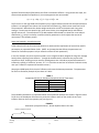
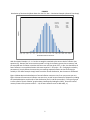
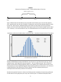
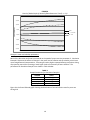
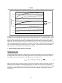
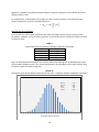
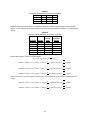
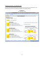
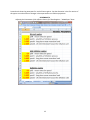
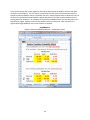
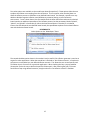
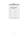
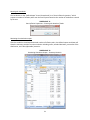
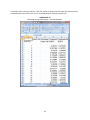
A USER’S GUIDE TO
THE INFLATION GENERATOR
Sponsored by
Casualty Actuarial Society
Canadian Institute of Actuaries
Society of Actuaries
Kevin C. Ahlgrim
Associate Professor
Illinois State University
Department of Finance, Insurance and Law
340 State Farm Hall of Business – Campus Box 5480
Normal, IL 61790-5480
(309) 438-2727
[email protected]
Stephen P. D’Arcy
Professor Emeritus
University of Illinois at Urbana-Champaign
435 Wohlers Hall
1206 South Sixth Street
Champaign, IL, 61820
(217) 333-0772
[email protected]
February 2012
Document 212088
© 2012 Casualty Actuarial Society, Canadian Institute of Actuaries, and Society of Actuaries, All Rights Reserved
The opinions expressed and conclusions reached by the authors are their own and do not represent any official position or
opinion of the sponsoring organizations or their members. The sponsoring organizations make no representation or warranty to
the accuracy of the information.
A USER’S GUIDE TO THE INFLATION GENERATOR
The level and change of the rate of inflation is an important assumption in many actuarial models. The
rate of inflation can affect the level of future claims, the demand for new policies, as well as affect the
level of interest rates or returns on assets. This paper documents the inflation generator that has been
developed for the sponsoring organizations and is available for a variety of actuarial applications. The
model simulates the general inflation rate and the user may wish to translate the general inflation rate
to other rates such as line of business inflation.
The paper is organized as follows. The first section describes a general process for inflation that is used
in the spreadsheet model. This section focuses on explaining the effects of changes in the model’s
parameters on inflation projections. The second section provides more details about the inflation
generator when using monthly time steps in the simulation. The third section discusses regime
switching where the inflation process is modified based on potential structural changes in the economic
environment. Finally, we illustrate the inflation generator with actual screenshots from the spreadsheet
model.
1. MEAN REVERTING INFLATION UNDER ANNUAL TIME STEPS
A mean reverting process
There are many possible formulations of an inflation model. The inflation generator uses an OrnsteinUhlenbeck process which is based on changes in the inflation rate. The continuous time OrnsteinUhlenbeck process is:
𝑑𝑞𝑡 = 𝑘(𝜃 − 𝑞𝑡 )𝑑𝑡 + 𝜎𝑑𝐵𝑡
(1)
This process is a mean reverting process since the level of inflation tends toward some average level
denoted by 𝜃. The first term on the right hand side of equation (1) is called the drift and it indicates the
expected change in the level of inflation over the next interval of time. The second term is called the
diffusion and it represents the volatility, or stochastic component of future inflation.
To understand the mean reverting process, consider the case where the current level of inflation (𝑞𝑡 ) is
below its mean, so that (𝑞𝑡 < 𝜃). In this case, the drift is positive, which indicates that inflation is
expected to increase next period. How quickly the rate of inflation reverts to its mean is determined by
the speed parameter 𝑘. As the drift pulls inflation toward 𝜃, there is uncertainty in the environment
which is represented by changes in a Brownian motion (𝑑𝐵𝑡 ). The relative size of the parameters 𝑘 and
𝜎 affect the amount of randomness of the inflation process. If 𝜎 is large, the uncertainty exhibited by
the Brownian motion is magnified and any reversion toward the mean inflation rate may be
overshadowed by the diffusion process. However, if 𝑘 increases (relative to 𝜎), then mean reversion
dominates the movement of inflation.
Though continuous time processes are useful for deriving analytical results such as the average future
inflation rate, actuaries often use discrete time simulations when performing cash flow testing or
2
dynamic financial analysis (DFA) where cash flows are related to inflation. Using annual time steps, the
discrete time equivalent of equation (1) is an autoregressive time series model:
𝑞𝑡+1 = 𝑞𝑡 + 𝑑𝑞𝑡 = [(1 − 𝑘)𝑞𝑡 + 𝑘𝜃] + 𝜎𝜀𝑡
(2)
The first term on the right hand side of equation (2) (in square brackets) shows that the expected future
inflation is an average of two values: the current level of inflation (𝑞𝑡 ) and the mean reversion level 𝜃.
The parameter 𝑘 determines the relative weight attached to current environment and a long-term
average. If mean reversion speed is high, then recent history is not weighted heavily and inflation
quickly reverts to 𝜃. The second term in (2) adds random shocks based on a draw from a normalized
distribution (𝜀𝑡 ), which is scaled by a constant volatility parameter 𝜎 which adjusts the amount of
uncertainty in the inflation process.
Numerical examples – Annual time steps
A few examples will help illustrate how equation (2) works and the implications of each of the model’s
parameters on projected inflation levels. (NOTE: In the examples that follow, the parameters are
chosen for illustration purposes only to isolate the effects of each parameter.)
In the first example, the mean reversion speed is set at a high level which weights the long-term average
heavily when projecting future inflation. (It might be noted that with a discrete time process with
annual time steps, choosing a mean reversion speed greater than 1.0 leads to excessive fluctuations in
inflation by creating a “reflective” process. If 𝑘 > 1.0 and the current level of inflation is below its mean,
next year’s inflation is expected to exceed the mean.)
We project 10,000 paths for the level of inflation under several alternate parameters. The parameters
for the first simulation (Example A) are shown in Table 1.
TABLE 1
Sample Parameters for Simulation Example A (Annual Time Steps)
Variable
Value
1.0
𝑘
3.00%
𝜃
4.00%
𝜎
Initial inflation
1.00%
The probability distribution of projected inflation from Simulation Example A is shown in Figure 2 below.
To be clear, the distribution illustrates one particular inflation rate from the model, the one-year
inflation rate over the first projection year (see Figure 1).
FIGURE 1
Illustration of Projection Period – Annual Inflation Rate in One Year
Inflation projection period
Starting
Point
Year 1
Year 2
3
Year 3
4
FIGURE 2
Distribution of the Annual Inflation Rate Over the First Year – Simulation Example A (Annual Time Steps)
-12.05%
18.50%
3.00%
4.00%
10,000
-15%
-14%
-13%
-12%
-11%
-10%
-9%
-8%
-7%
-6%
-5%
-4%
-3%
-2%
-1%
0%
1%
2%
3%
4%
5%
6%
7%
8%
9%
10%
11%
12%
13%
14%
15%
16%
17%
18%
19%
20%
Frequency
Minimum
Maximum
Mean
Std. Dev.
# of Sims
Annual Inflation Rate Over the First Year
With Simulation Example A, 𝑘 = 1.0 so that no weight is attached to the current level of inflation (see
equation (2)). Because the mean reversion speed is so high, the inflation process has no memory and
the expected rate of inflation coincides with the mean reversion level of 3%. In fact, the distribution of
future inflation is a normal distribution with mean equal to 𝜃 = 3% and 𝜎 = 4%. Changing the volatility
parameter (𝜎) simply affects the uncertainty surrounding expected inflation so that increasing the
volatility in the above example simply leads to a wider normal distribution, but the mean is unaffected.
Figure 3 below depicts the distribution of annual inflation rates over time, from year one to year ten.
Figure 3 shows the mean annual inflation rate over time, as well as two measures of dispersion including
the standard deviation and the tails of the distribution (the 5th and 95th percentiles). This type of graph
is often called a “funnel of doubt” graph and was introduced by Redington (1952). Given the limited
memory feature of the process when 𝑘 = 1.0, all future inflation rates are Normal(𝜃, 𝜎).
5
FIGURE 3
Funnel of Doubt Graph of Annual Inflation Rates over Time – Simulation Example A (Annual Time Steps)
10,00%
8,00%
Annual Inflation Rate
6,00%
4,00%
Mean
+ / - 1 Std. dev.
5% - 95%
2,00%
0,00%
-2,00%
-4,00%
Yr 1
Yr 2
Yr 3
Yr 4
Yr 5
Yr 6
Yr 7
Yr 8
Yr 9
Yr 10
Simulation Example A generates a simple distribution for future inflation, but it is likely that the
expected path of inflation does place weight on history. While central bankers may employ various
tools of monetary policy to keep inflation around an established target level of inflation, these tools take
time to propagate through the economy. In fact, excessive use of monetary policy tools may lead to
increased economic volatility. Therefore, it is reasonable to assume that the expected future rate of
inflation adjusts more slowly over time, with some weight attached to current inflation levels. To
incorporate the more modest change in inflation over time, we lower the level of mean reversion speed
for Simulation Example B. In order to compare the results to the previous projections, all of the
remaining parameters are left unchanged.
TABLE 2
Sample Parameters for Simulation Example B (Annual Time Steps)
Variable
Value
0.5
𝑘
3.00%
𝜃
4.00%
𝜎
Initial inflation
1.00%
Using these parameters, each year the rate of inflation is expected to move only half of the distance
from its current value of 1.0% toward the reversion level of 3.0%. For Simulation Example B, annual
inflation over the next year still has a normal distribution since the source of randomness in equation (2)
is 𝜀, a standard normal variate. Figure 4 illustrates the distribution of projected inflation next year,
which is normal with a mean of 2% and a standard deviation equal to the volatility parameter of 4%.
6
FIGURE 4
Distribution of the Annual Inflation Rate over the First Year – Simulation Example B (Annual Time Steps)
19%
17%
15%
-15.53%
18.38%
2.00%
4.00%
10,000
13%
11%
9%
7%
5%
3%
1%
-1%
-3%
-5%
-7%
-9%
-11%
-13%
-15%
Frequency
Minimum
Maximum
Mean
Std. Dev.
# of Sims
Annual Inflation Rate Over the First Year
Figure 5 is the funnel of doubt graph for Simulation Example B and the only apparent difference is the
slow increase in the mean level inflation over the next 10 years since each year the expected level of
inflation moves half of the way from its current level to the mean level of 3%. Upon further inspection
of Figure 5, it becomes clear that the volatility also grows slightly as we project further into the future.
FIGURE 5
Funnel of Doubt Graph of Annual Inflation Rates over Time – Simulation Example B (Annual Time Steps)
12,00%
10,00%
Annual Inflation Rate
8,00%
6,00%
4,00%
Mean
+ / - 1 Std. Dev.
2,00%
5% - 95%
0,00%
-2,00%
-4,00%
-6,00%
Yr 1
Yr 2
Yr 3
Yr 4
Yr 5
Yr 6
Yr 7
Yr 8
Yr 9
Yr 10
Let us look more closely at the one-year inflation rate in the second projection year (depicted in Figure 6
below).
7
FIGURE 6
Illustration of Projection Period – Annual Inflation Rate in Two Years
Inflation projection period
Starting
Point
Year 1
Year 2
Year 3
Figure 7 below shows the distribution of the projected annual inflation rate in the second projection
year. Note that each year the rate of inflation is expected to move half of the distance toward its mean
level of 3%. After one year, expected inflation moves from the initial level of 1% to 2% (as shown
above), and in the second year (expected) inflation again moves half its distance toward 3%, from 2% to
2.5%. However, in the second projection year, the standard deviation has increased from 4% to 4.47%.
FIGURE 7
Distribution of the Annual Inflation Rate in the Second Year – Simulation Example B (Annual Time Steps)
-14.32%
20.54%
2.50%
4.47%
10,000
-15%
-14%
-13%
-12%
-11%
-10%
-9%
-8%
-7%
-6%
-5%
-4%
-3%
-2%
-1%
0%
1%
2%
3%
4%
5%
6%
7%
8%
9%
10%
11%
12%
13%
14%
15%
16%
17%
18%
19%
20%
21%
22%
23%
24%
25%
Frequency
Minimum
Maximum
Mean
Std. Dev.
# of Sims
Annual Inflation Rate Over the Second Year
When making longer-term inflation projections in Simulation Example A, there was no difference
between the distribution of projected inflation in the first year vs. any other future year (e.g., the 10th
projection year). With high mean reversion speed (𝑘 = 1.0) , the inflation process “lost” its memory
quickly since there was no weight applied to history; any random noise created by the economy in the
first projection year was completely forgotten when projecting inflation in future years. As a result, the
standard deviation of the distribution of future inflation rates was completely driven by the
contemporaneous uncertainty inherent in the economy.
But when the speed of reversion is slower, the inflation process remembers the uncertainty of the past
so that outliers in early projection years carry over to future years. In Simulation Example B, future
8
inflation is based on the existing level of inflation and the assumed long-run mean. And the volatility of
future inflation increases because it reflects the uncertainty inherent in the projection period is
weighted with the volatility exhibited in previous periods. To give an economic interpretation,
policymakers must deal with the imprecise data of the current period, as well as consider the
significance of noisy past data.
This growth in volatility is not unbounded for longer projection periods. As long as some weight is
attached to a target mean reversion level, the increase in volatility is limited since historical levels of
inflation become less relevant as the projection period increases. Miller and Wichern (1977) show how
the volatility of an autoregressive process increases with the projection period. In particular, they
calculate the volatility limit for long projection periods. As the projection period (𝑡) increases, Miller and
Wichern (1977) find the limit of volatility for an autoregressive process with annual time steps (such as
equation (2)) is:
𝑉𝑜𝑙𝑎𝑡𝑖𝑙𝑖𝑡𝑦 𝑞𝑡 →
𝜎
�1−(1−𝑘)2
Table 3 illustrates the growth of volatility by projection period and the effects of varying the speed of
mean reversion of the inflation process. When the mean reversion speed is high (Simulation
Example A), the process has memory loss and as the projection period grows, volatility is tied to the
current environment. However, when 𝑘 is low, the inflation process is less tethered to an average
inflation level and uncertainty grows.
TABLE 3
Comparison of Volatility by Projection Period
Std. Dev.
Std. Dev.
Std. Dev.
of Inflation
of Inflation
of Inflation
Projection Year
(𝒌 = 𝟏. 𝟎)
(𝒌 = 𝟎. 𝟓)
(𝒌 = 𝟎. 𝟏)
1
4.00%
4.00%
4.00%
2
4.00
4.47
5.38
3
4.00
4.58
6.28
4
4.00
4.61
6.93
5
4.00
4.62
7.41
6
4.00
4.62
7.77
7
4.00
4.62
8.06
8
4.00
4.62
8.28
9
4.00
4.62
8.46
10
4.00
4.62
8.60
⁞
⁞
⁞
⁞
∞
4.00
4.62
9.18
Figure 8 below translates this growth in volatility to a funnel of doubt graph for a simulation with
𝑘 = 0.1. Comparing Figure 8 to earlier funnel of doubt graphs (Figures 3 and 5), we can see how
uncertainty changes with the mean reversion speed.
9
(3)
FIGURE 8
Funnel of Doubt Graph of Annual Inflation Rates over Time (𝑘 = 0.1)
20,00%
15,00%
Annual Inflation Rate
10,00%
5,00%
Mean
+ / - 1 Std. Dev.
0,00%
5% - 95%
-5,00%
-10,00%
-15,00%
Yr 1
Yr 2
Yr 3
Yr 4
Yr 5
Yr 6
Yr 7
Yr 8
Yr 9
Yr 10
Changes in mean and volatility parameters
Much of the discussion until now has centered on the speed of mean reversion parameter 𝑘. Simulation
Example C illustrates the effects of changes in the mean level of inflation and the volatility, which have
more straightforward interpretations. Increasing 𝜃 leads to higher expected inflation projections during
all projection years while increasing 𝜎 leads higher levels of uncertainty of future inflation. The
parameters for Simulation Example C are shown in Table 4 below:
TABLE 4
Sample Parameters for Simulation Example C
Variable
Value
0.3
𝑘
10.00%
𝜃
6.00%
𝜎
Initial inflation
1.00%
Figure 9 is the funnel of doubt graph showing the distribution of annual inflation rates for years one
through 10.
10
FIGURE 9
Funnel of Doubt Graph of Annual Inflation Rates over Time – Simulation Example C (Annual Time Steps)
25,00%
20,00%
Annual Inflation Rate
15,00%
10,00%
Mean
+ / - 1 Std. dev.
5,00%
5% - 95%
0,00%
-5,00%
-10,00%
Yr 1
Yr 2
Yr 3
Yr 4
Yr 5
Yr 6
Yr 7
Yr 8
Yr 9
Yr 10
As expected, the average inflation level slowly increases toward 10% over the projection period. If the
modeler wants to have expected inflation move more quickly to 10%, he or she can increase the mean
reversion speed. In addition, the standard deviation of the distribution starts out at 6% and increases
slightly over the remaining projection period. Based on the discussion of the two previous example
simulations, the annual inflation rate in the first projection year has a normal distribution with mean of
3.7% and a standard deviation of 6.00% (𝜎). The mean is 3.7% since it is 30% of the way from the initial
rate of 1% toward the long-term mean level of 10%. In the 10th projection year, the mean simulated
level of inflation is 9.75% and the standard deviation is 8.43%.
2. MEAN REVERSION WITH MONTHLY TIME STEPS
Changing the time step
The discussion above uses examples with annual time steps to help illustrate the basic operation of an
autoregressive model. However, the inflation generator uses monthly time steps to project inflation.
Extending the discrete autoregressive model (2) to shorter time steps yields:
𝑞𝑡+∆𝑡 = {[1 − 𝑘(∆𝑡)]𝑞𝑡 + 𝑘(∆𝑡)𝜃} + �𝜎√∆𝑡�𝜀𝑡
(4)
With annual time steps, it was easier to see the impact of the speed of reversion parameter (𝑘) since it
could be directly interpreted as the weighting applied to the mean reversion level (see equation (2)).
Thus, when 𝑘 = 1.0 and there are annual time steps, the process has no memory since there is no weight
attached to previous inflation values. But when the time step is reduced, things become a bit more
complicated.
11
Consider how the expected inflation rate is affected if we iterate (4) when 𝑘 = 1.0 using semiannual time
steps (∆𝑡 = 0.5). The expected inflation becomes:
𝐸(𝑞0.5 ) = {[1 − 𝑘(∆𝑡)]𝑞0 + 𝑘(∆𝑡)𝜃}
= 0.5 × 1% + 0.5 × 3% = 2.0%
(5)
𝐸(𝑞1.0 ) = {[1 − 𝑘(∆𝑡)]𝑞0.5 + 𝑘(∆𝑡)𝜃}
= 0.5 × 2% + 0.5 × 3% = 2.5%
Since 𝑘 = 1.0, inflation does move toward the mean reversion level of 3.0%. But since the time steps are
semiannual, inflation moves only half of that distance during each time step. After two semiannual time
steps, the expected inflation rate is 2.5%. Compare this to the annual time step process with the same
parameters, where expected inflation would have moved fully to its mean reversion level. To project
future inflation, we iterate equation (4):
𝑠
𝐸(𝑞𝑡+𝑠∆𝑡 ) = [1 − 𝑘(∆𝑡)]𝑠 × 𝑞𝑡 + �1 − �1 − 𝑘(∆𝑡)� � × 𝜃
for 𝑠 = 1, 2, …
(6)
While future inflation is still a weighted average of past values and the mean reversion level, the annual
mean reversion speed has less direct interpretation and subsequent inflation projections are affected.
The inflation process (𝑞𝑡 ) vs. observed annualized inflation (𝜑𝑡,𝑡+𝑠 )
Equation (6) determines the level of the expected inflation process (𝑞) at some future time period.
When ∆𝑡 < 1.0, we need to make a distinction between expressing the value of the contemporaneous
inflation process vs. expressing annualized inflation. The inflation generator uses monthly time steps, so
the expected value of the inflation process (𝑞) from equation (6) only affects price levels for one month.
However, when discussing inflation, it is common to think of the annual change in prices from one year
to the next. This view of inflation is an historical, cumulative effect of the inflation process over 12
consecutive months.
To illustrate the difference, first define 𝜑𝑡,𝑡+𝑠 as the observed and annualized inflation rate over an
𝑠-year period, from time 𝑡 to time 𝑡 + 𝑠, where 𝑠 > 0. A common way to measure 𝜑𝑡,𝑡+𝑠 is by
determining the percentage change in the level of prices as measured by the consumer price index (CPI):
𝑠
�1 + 𝜑𝑡,𝑡+𝑠 � =
𝐶𝑃𝐼𝑠
𝐶𝑃𝐼𝑡
Now suppose we wanted to use the inflation generator to estimate the rate of inflation during the first
projection year. To calculate this value (denoted 𝜑0,1 ), we need to compound the simulated value of
the inflation process each month over the next 12 months. Let 𝑞1/12, 𝑞2/12 , …, 𝑞12/12, be the sampled
inflation process from (4) using monthly time steps. Then,
1/12
�1 + 𝑞1/12 �
1/12
�1 + 𝑞2/12 �
1/12
… �1 + 𝑞12/12 �
= 1 + 𝜑0,1
In the simulations performed in the prior section using annual time steps, there was no need to
distinguish the inflation process and the reported rate of inflation since they were identical. But
12
(7)
equation (7) indicates that observed annual inflation is based on projections of the inflation process at
different points in time.
For completeness, as the number of time steps in a year increases, the limit is the continuous time
model in equation (1) and the annualized inflation is:
1
1 + 𝜑0,1 = 𝑒𝑥𝑝 �� 𝑞𝑡 𝑑𝑡�
0
Monthly time step simulations
In this section, we run the same simulations that were illustrated in the first section using the same
parameters. However, as in the inflation generator, in this section we use monthly time steps instead of
annual time steps.
TABLE 5
Sample Parameters for Simulation Example A (Monthly Time Steps)
Variable
Value
1.0
𝑘
3.00%
𝜃
4.00%
𝜎
Initial inflation
1.00%
Figure 10 illustrates the distribution of the annual inflation rate resulting from 10,000 projections paths
of the monthly inflation process. (For comparative purposes, the distribution of first year inflation using
annual time steps was shown in Figure 2.)
FIGURE 10
Distribution of the Annual Inflation Rate over the First Year – Simulation Example A (Monthly Time Steps)
-4.72%
8.63%
1.80%
1.77%
10,000
Annual Inflation Rate Over the First Year
13
9.0%
8.5%
8.0%
7.5%
7.0%
6.5%
6.0%
5.5%
5.0%
4.5%
4.0%
3.5%
3.0%
2.5%
2.0%
1.5%
1.0%
0.5%
0.0%
-0.5%
-1.0%
-1.5%
-2.0%
-2.5%
-3.0%
-3.5%
-4.0%
-4.5%
Frequency
Minimum
Maximum
Mean
Std. Dev.
# of Sims
Note that the mean value of annualized inflation is 1.80%, which is significantly lower than the case with
annual time steps (3.00%) for two reasons. First, as illustrated in the example in equation (5), when
moving to shorter time steps the interpretation of the mean reversion speed parameter 𝑘 is changed.
One way that is helpful to interpret the speed of mean reversion of the inflation process (𝑞) toward its
long-term average is its “half-life,” or the time it takes to move one-half of the way to the mean
reversion level.
Half-life (# of periods) =
ln (0.5)
ln [1−𝑘(∆𝑡)]
(8)
When 𝑘 = 1.0 with annual time steps, inflation was expected to move to the reversion level of 3% next
period. However, with monthly time steps (∆𝑡=1/12), equation (8) shows that it takes approximately 8
months for the inflation process to make it half of the distance toward 3%. In fact, Table 6 shows the
expected value of the inflation process (𝑞𝑡 ) from Simulation Example A for each month during the first
year.
TABLE 6
Expected Path of Inflation Process – Simulation Example A (Monthly Time Steps)
Expected Value of
Month
Inflation Process (𝒒)
Initial
1.00%
1
1.17%
2
1.32%
3
1.46%
4
1.59%
5
1.71%
6
1.81%
7
1.91%
8
2.00%
9
2.09%
10
2.16%
11
2.23%
12
2.30%
The second difference in expected inflation when using monthly time steps is that Figure 10 shows the
distribution of 𝜑0,1 which is the cumulative change in prices over the first year. Equation (7) shows that
the construction of the annualized inflation rate is developed from the projections of the monthly
inflation process. Given that the inflation process starts at 1% and is expected to move to monthly
toward 3% slowly over time according to Table 6, it turns out the average inflation rate over this first
year is 1.80%.
The funnel of doubt graph for Simulation Example A under monthly time steps is shown in Figure 11.
The rate of annual inflation slowly increases toward 3% each year (as expected).
14
FIGURE 11
Funnel of Doubt Graph of Annual Inflation Rates over Time – Simulation Example A (Monthly Time Steps)
8,00%
7,00%
6,00%
Annual Inflation Rate
5,00%
4,00%
Mean
3,00%
+ / - 1 Std. dev.
5% - 95%
2,00%
1,00%
0,00%
-1,00%
-2,00%
Yr 1
Yr 2
Yr 3
Yr 4
Yr 5
Yr 6
Yr 7
Yr 8
Yr 9
Yr 10
Figure 10 also states the standard deviation of the first year inflation rate as 1.77%, again lower than the
4.00% when using annual time steps. With annual time steps and 𝑘 = 1.0, uncertainty in future inflation
was driven completely by the volatility parameter 𝜎 since there was no distinction between 𝑞 and 𝜑.
Two forces influence the volatility when changing to monthly time steps.
First, the volatility of the monthly inflation process is now scaled by the time step (𝜎√∆𝑡) and while
Figure 11 shows that the volatility increases over time, it is less than the volatility parameter of the
inflation process (𝜎 = 4%). As forecast period is extended, equation (3) illustrates how the volatility of
𝑞𝑡 grows and if we restate equation (3) with monthly time steps:
𝑉𝑜𝑙𝑎𝑡𝑖𝑙𝑖𝑡𝑦 𝑞𝑡 →
𝜎√∆𝑡
�1−[1−𝑘(∆𝑡)]2
(9)
In Simulation Example A, this limit of volatility is 2.89%. Thus, for very long term projections of 𝑞𝑡 , the
standard deviation is approximately 2.89%, less than the volatility with annual time steps.
As explained earlier, the relative sizes of the mean reversion speed and the volatility parameters work
together to determine the amount of randomness in inflation. In Simulation Example A, the high level of
mean reversion dampens the effects of uncertainty over time. If there is a month where the random
shock happens to be an outlier, the high level of mean reversion quickly brings inflation back toward 𝜃.
This dramatically reduces the amount of uncertainty in inflation over any period of time. However, as
the size of mean reversion falls (relative to 𝜎), outliers can compound and lead to more uncertainty
when predicting inflation. Table 7 shows the effects of reducing mean reversion speed on long-term
inflation projections as determined by equation (9):
15
TABLE 7
Limit of Volatility of Inflation Process
Volatility limit (eq. (9))
𝒌
1.0
2.89%
0.5
4.04%
0.3
5.20%
0.2
6.35%
0.1
8.96%
The second factor affecting the volatility of annual inflation depicted in Figures 10 and 11 is based
equation (7), which is the product of the monthly inflation process. The standard deviation of
annualized inflation is based on the volatility of a product of the inflation process each month.
Goodman (1962) provides a general analytic solution to the variance of the product of random variables.
The numerical solution for the standard deviation of 𝜑0,1 is 1.77% as shown in Figure 10. In the 10th
projection year, the standard deviation is 2.45%.
Simulation Example B lowers the mean reversion speed.
TABLE 8
Sample Parameters for Simulation Example B (Monthly Time Steps)
Variable
Value
0.5
𝑘
3.00%
𝜃
4.00%
𝜎
Initial inflation
1.00%
Figure 12 illustrates the distribution of the projected inflation in the first year and Figure 13 provides the
funnel of doubt graph for Simulation Example B using monthly time steps.
16
FIGURE 12
Distribution of the Annual Inflation Rate over the First Year – Simulation Example B (Monthly Time Steps)
-5.94%
9.96%
1.46%
2.08%
10,000
9.5%
10.0%
9.0%
8.5%
8.0%
7.5%
7.0%
6.5%
6.0%
5.5%
5.0%
4.5%
4.0%
3.0%
3.5%
2.5%
2.0%
1.5%
1.0%
0.5%
0.0%
-0.5%
-1.0%
-1.5%
-2.0%
-2.5%
-3.0%
-3.5%
-4.0%
-4.5%
-5.0%
-5.5%
Frequency
Minimum
Maximum
Mean
Std. Dev.
# of Sims
Annual Inflation Rate Over the First Year
FIGURE 13
Funnel of Doubt Graph of Annual Inflation Rates over Time – Simulation Example B (Monthly Time Steps)
10,00%
8,00%
Annual Inflation Rate
6,00%
4,00%
Mean
+ / - 1 Std. dev.
2,00%
5% - 95%
0,00%
-2,00%
-4,00%
Yr 1
Yr 2
Yr 3
Yr 4
Yr 5
Yr 6
Yr 7
Yr 8
Yr 9
Yr 10
Note that when the reversion speed is lowered, it takes more time for inflation to move toward 𝜃 and
the volatility of inflation is higher.
17
The results of Simulation Example C are quickly shown in Figure 14.
TABLE 9
Sample Parameters for Simulation Example C (Monthly Time Steps)
Variable
Value
0.3
𝑘
10.00%
𝜃
6.00%
𝜎
Initial inflation
1.00%
FIGURE 14
Funnel of Doubt Graph of Annual Inflation Rates over Time – Simulation Example C (Monthly Time Steps)
25,00%
Annual Inflation Rate
20,00%
15,00%
Mean
10,00%
+ / - 1 Std. dev.
5% - 95%
5,00%
0,00%
-5,00%
Yr 1
Yr 2
Yr 3
Yr 4
Yr 5
Yr 6
Yr 7
Yr 8
Yr 9
Yr 10
3. REGIME SWITCHING
When developing models for economic and financial variables, history is often used as a metric of model
performance. Often there exists historical subperiods that occur during structural transitions in the
economy or during financial crises and the historical fit of models may be lacking.
Consider term structure models which aim to mimic interest rate movements. When measuring the
relative performance of several models (such as in Chan, Karolyi, Longstaff, and Sanders (1992)), most
popular models fail to capture the interest rate dynamics exhibited during the early 1980s. But the
higher levels of interest rates and the increase in volatility of this period may be caused by a shift in the
policies of the Federal Reserve to target money growth. In situations where there are distinct episodes
where the behavior of time series appears markedly distinctive, modelers may consider a change in
regime. Hamilton (1989) provides a general discussion of regime switching and Ang and Bekaert (2002)
describe an application to term structure models. The economic rationale for regime switching is that at
any point in time, the dynamics of a model are dictated by a particular regime. But changes in the
economy may build such that the assumed process for financial variables is no longer appropriate. In
18
these cases, the economy is said to switch regimes. In an alternate regime, the dynamics of financial
models differ from those assumed under a normal economic environment.
As another example of regime switching models, Hardy (2001) discusses a regime switching model for
stock returns as a way to capture the fatter tails exhibited in historical returns. In normal economic
times, equity returns may be approximately normal with a constant variance, but during times of severe
economic uncertainty and recession observed returns from a normal distribution might appear
statistically improbable. To handle these outliers, Hardy (2001) introduces a second regime which
incorporates increased uncertainty. Typically, to keep models tractable, regimes are defined
somewhat broadly so that the number of changes in a given period remains relatively low. For example,
Hardy (2001) uses only two regimes and finds that extending the stock return model to three regimes
yields only a marginal improvement in statistical fit for US data.
The inflation generator uses an autoregressive process to project future inflation rates. When selecting
parameters for this process, users might choose values that yield a model that mimics historical
inflation. But future economic conditions have the potential to move inflation in ways that have not
been observed in the short history embedded in US data. In addition to “normal” inflation, we see two
other possible regimes which are plausible. First, actions of the Federal Reserve targeted to stimulate
the economy may create increased price pressures in the economy that could generate higher inflation
than observed recently. Alternatively, if the actions of the Federal Reserve fail to stimulate significant
economic activity or if the world economy continues to retrench, decreased demand may increase the
potential for deflationary environments.
Given these other possible scenarios, the inflation generator uses three regimes. In each regime
inflation follows an autoregressive process, but at any point in time the dynamics of the inflation
process are dictated by the parameters of the prevailing regime. Changes in regime are based on
transition (or switching) probabilities. Selecting transition probabilities is an important but difficult task
given the inability to pinpoint specific regimes in historical data since we cannot directly observe
changes in regimes but instead must imply them. Even when the level of inflation has been observed to
be “low” relative to historical standards, this does not mean that the economy has entered the
deflationary regime period; an alternative explanation is that the normal regime has just experienced an
outlier. Single outliers are temporary, but regimes tend to persist.
The transition probabilities directly determine the expected length of time in a particular regime.
Suppose the economy is currently in the “normal” regime. Denote 𝜋 as the probability of staying in the
normal regime next period. Therefore, the probability of switching to either to a high inflation regime or
to a deflation regime is (1 − 𝜋). We can determine the probability that the current regime lasts for
exactly five periods:
𝑃𝑟𝑜𝑏𝑎𝑏𝑖𝑙𝑖𝑡𝑦 𝑜𝑓 𝑟𝑒𝑔𝑖𝑚𝑒 𝑑𝑢𝑟𝑎𝑡𝑖𝑜𝑛 𝑜𝑓 𝑓𝑖𝑣𝑒 𝑝𝑒𝑟𝑖𝑜𝑑𝑠 = 𝜋 4 (1 − 𝜋)
In fact, the expected (mean) number of periods for the regime duration is
𝑡−1
∑∞
× (1 − 𝜋) =
𝑡=1 𝑡 × 𝜋
1
1−𝜋
(10)
To understand how the transition probabilities affect the regime duration, consider Table 10. The first
column lists the probability of remaining in a particular regime from month to month, denoted as 𝜋
19
above. The second column provides another interpretation by simply restating this probability another
way: the probability of switching regimes within a year. The third column uses equation (10) to derive
the mean duration in a particular regime. But since the probability distribution of a regime’s duration is
positively skewed, the last column also shows the median duration of a regime. Table 10 may be helpful
for users choosing transition probabilities for the inflation generator.
TABLE 10
Transition Probabilities and Regime Duration
Annual
Monthly
Equivalent
Mean
Median
Likelihood of
Switching
(In years) (In years)
Remaining
99.9%
1.2%
83.33
57.73
99.8%
2.4%
41.67
28.85
99.7%
3.5%
27.78
19.23
99.6%
4.7%
20.83
14.41
99.5%
5.8%
16.67
11.52
99.4%
7.0%
13.89
9.60
99.3%
8.1%
11.90
8.22
99.2%
9.2%
10.42
7.19
99.1%
10.3%
9.26
6.39
99.0%
11.4%
8.33
5.75
98.9%
12.4%
7.58
5.22
98.8%
13.5%
6.94
4.79
98.7%
14.5%
6.41
4.41
98.6%
15.6%
5.95
4.10
98.5%
16.6%
5.56
3.82
98.4%
17.6%
5.21
3.58
98.3%
18.6%
4.90
3.37
98.2%
19.6%
4.63
3.18
98.1%
20.6%
4.39
3.01
98.0%
21.5%
4.17
2.86
A regime switching example
To show how regime switching is incorporated in the inflation generator, we walk through a sample
path that illustrates a regime shift. The inflation generator uses three regimes and at any point in time,
the inflation process follows an autoregressive model like equation (4) using monthly time steps.
However, if there is a regime change in the economy, the parameters of the process change. Table 11
shows one example of parameters for the three regimes.
20
TABLE 11
Parameters for Regime Shift Simulation Example
Regime
𝒌
𝜽
𝝈
Normal
1.0
3.5%
5.0%
High
0.4
9.0%
3.0%
Deflation 0.6 -3.0% 3.0%
Table 12 shows one sample path in a simulation, where the inflation process begins in the “normal”
regime. In this example, after three months it turns out that the economy switches to a “high inflation”
regime.
TABLE 12
Month by Month Projection for a Single Projection
Time Step
0
1/12
2/12
3/12
4/12
5/12
Regime
Normal
Normal
Normal
Normal
High
High
Normal
Draw
-0.41144
-0.13124
1.29302
-0.15564
0.52153
Simulated
Annualized
Inflation
1.00%
0.61%
0.67%
2.77%
1.48%
2.18%
We simulate inflation for the next five months:
𝑞𝑡 + 𝑘(𝜃 − 𝑞𝑡 )∆𝑡 + 𝜀𝑡 𝜎√∆𝑡 = 𝑞𝑡+1
Month 1: 1.00% + 1.0 × (3.50% − 1.00%) ×
Month 2: 0.61% + 1.0 × (3.50% − 0.61%) ×
Month 3: 0.67% + 1.0 × (3.50% − 0.67%) ×
1
1
− 0.41144 × 5.0% × � = 0.61%
12
12
1
1
− 0.13124 × 5.0% × � = 0.61%
12
12
1
1
+ 1.29302 × 5.0% × � = 2.77%
12
12
After the third month, we switch regimes and therefore, the parameters of the autoregressive inflation process
change.
Month 4: 2.77% + 0.4 × (9.00% − 2.77%) ×
Month 5: 1.48% + 0.4 × (9.00% − 1.48%) ×
21
1
1
− 0.15564 × 3.0% × � = 1.48%
12
12
1
1
+ 0.52153 × 3.0% × � = 2.18%
12
12
4. USING THE INFLATION GENERATOR
This section walks the user through the inflation generator spreadsheet. To run the inflation generator,
the user must complete the following steps:
1. Open the inflation model spreadsheet and enable the macros.
2. Review and adjust the model’s parameters on the “ModelInput” sheet (if desired).
3. Select the cells of interest to track during the simulation (select output cells).
4. Run the simulation.
5. Review the output.
The following documentation walks the user through these steps.
Loading the inflation model
After opening the spreadsheet you will have to enable the embedded macros. Depending on your
version of Excel, you may get a popup window or a security warning near the top of the screen (shown
as Screenshot #1 below) asking to enable the macro content.
SCREENSHOT 1
Enable Macro Content (from Excel 2007)
After the macros have been enabled, the user must accept the legal disclaimer before continuing to the
model input sheet.
22
Adjusting the parameters - The “ModelInput” sheet
This section of the documentation walks you through each of the inputs on the “ModelInput” sheet
(Screenshot 2) so that users can adjust the parameters of the model, if desired.
SCREENSHOT 2
The “ModelInput” Sheet
23
The top left of the screen (Screenshot 3) asks the user to initialize the current inflation environment.
The default regime is checked as “Normal”, but the user can click on any of the other radio buttons to
begin simulations in an alternate regime. In addition, the most recent value for the level of inflation
should be entered (labeled “qinit” in Screenshot3).
SCREENSHOT 3
Initializing Current Inflation Environment – “ModelInput” sheet
As discussed above, the inflation generator is based on a regime switching process with three regimes.
One interpretation of these regimes is that when the US economy is experiencing “Normal” economic
times, the average inflation rate is considered moderate. But two other economic regimes are possible
in the future. First, expansionary fiscal policy combined with accommodative monetary policy may lead
to sustained inflationary pressures. In this “High” inflation regime, there is a significantly higher average
level of inflation than indicated from recent history. It seems plausible that in this high inflation regime,
volatility may also be higher. A second alternate regime is that of continued worldwide economic
stagnation despite government spending and central bank easing. The third regime incorporated in the
inflation model reflects the possibility of these deflationary pressures. In this regime, the average level
of inflation and the volatility are low.
24
Screenshot 4 shows the parameters for each of these regimes. See the discussion in the first section of
this paper to see the effects of changes in these parameters on inflation projections.
SCREENSHOT 4
Adjusting the Parameters of the Inflation Process for Three Regimes – “ModelInput” sheet
25
The transition among the various regimes is directed by two transition probability matrices and these
are shown in Screenshot 5. The first matrix is used for the first two years of the simulation while the
second transition probability matrix is used after year two. Having separate matrices allows the users to
tilt short-term probabilities toward specific regimes that the user may feel are warranted because of
existing economic conditions. For example, to increase the probabilities over the next two years to the
high inflation regime, adjust the short-term probability matrix to reflect this. After two years, the
regime switching probabilities of the second matrix are applied.
SCREENSHOT 5
Regime Transition Probability Matrices – “ModelInput” Sheet
26
Two other options are available on the model input sheet (Screenshot 6). These options allow the user
to adjust the inflation rate resulting from the simulations. The first option, when checked, does not
allow the inflation process to fall below a user defined lower bound. For example, a specific user may
decide to disallow negative inflation rates (deflationary scenarios) during a normal economic
environment. To use a lower bound, the user would check the lower bound box and enter the desired
lower bound as an additional parameter of the inflation process (see the parameters labeled “qlowN”,
“qlowH”, and “qlowD” in Screenshot 4). When the lower bound option is checked, if a simulated
interest rate falls below the user defined lower bound, the spreadsheet replaces the simulated inflation
rate with the desired lower bound.
SCREENSHOT 6
Other Options on the “ModelInput” Sheet
The second checkbox option shown in Screenshot 6 may be useful if the inflation generator is used as an
engine for other applications. When the second box is checked to “Set inflation scenario”, all stochastic
processes are overridden by a user defined inflation scenario. This allows the user to test specific path
of inflation that is of concern for a particular application. When checking the box, a pop-up window
(Screenshot 7) asks the user to define the specific inflation path. After entering the path, if the user
would like to stop using defined scenarios, simply unselect the “Set inflation scenario” checkbox.
27
SCREENSHOT 7
Defining Inflation Scenarios – “ModelInput” Sheet
28
Defining Output Cells
The sheet labeled “DefineOutput” contains three command buttons that execute macros to help users
track specific cells of interest, start a projection, and review simulation results (Screenshot 8).
SCREENSHOT 8
Three Macro Buttons for Tracking Output – “DefineOutput” Sheet
Before running a projection, the user will want to define the output cells of interest to track in the
simulation. When clicking the “Add Output Cell” button, a pop-up window (Screenshot 9) takes you to
the model’s inflation rate output and the user chooses a particular cell to follow.
SCREENSHOT 9
“Add Output Cell” Macro Button – Selecting an Inflation Rate
29
Note that in the example, the user is adding the one-year inflation rate that starts in ten years (see cell
F29 in Screenshot 10). Users can choose up to twenty variables to follow and after choosing a cell, these
variables of interest are shaded green.
SCREENSHOT 10
Selecting an Inflation Rate – Green Cells are Selected Output
If the user would like to clear all variables previously selected to start with a new batch of output
variables, click on button labeled “Clear All Output Cells” on the “DefineOutput” sheet (Screenshot 8).
30
Running the simulation
The last button on the “DefineOutput” sheet (Screenshot 8) is to “Start Inflation Projections,” which
projects a number of inflation paths over the next 50 years based on the number of simulations entered
by the user.
SCREENSHOT 11
Start Inflation Projections – Entering the Number of Paths
Reviewing the simulation output
After the model has simulated the desired number of inflation paths, the Define Output worksheet will
show the summary statistics from the simulation including mean, standard deviation, percentiles of the
distribution, and a few (adjustable) scenarios.
SCREENSHOT 12
Reviewing Simulation Output – Summary Statistics
31
Instead of just the summary statistics, if the user wishes to review all of the output (for each and every
simulated path), these can be seen on the “SimulationOutput” sheet (Screenshot 13).
SCREENSHOT 13
Reviewing Path by Path Output – “SimulationOutput”
32
Finally, the “StochasticProcess” sheet shows a bit of the internal operations of the model
(Screenshot 14). It illustrates one path of inflation including the simulated regime for each year. If the
user would like to simulate a single path at a time to see the model project, simply recalculate the
spreadsheet by hitting F9.
SCREENSHOT 14
Reviewing a Single Projection Path – “StochasticProcesses”
33
REFERENCES
Ang, Andrew and Geert Bekaert, 2002, "Regime Switches In Interest Rates," Journal of Business and
Economic Statistics 20 (2), 163-182.
Chan, K.C., G. Andrew Karolyi, Francis A. Longstaff, and Anthony B. Sanders, 1992, “An Empirical
Comparison of Alternative Models of the Short-Term Interest Rate,” Journal of Finance 47 (3):
1209-1227.
Goodman, L.A., 1962, “The Variance of the Product of K Random Variables,”Journal of the American
Statistical Association 57 (March), 54-60.
Hamilton, James D., 1989, “A New Approach to the Economic Analysis of Nonstationary Time Series and
the Business Cycle,” Econometrica 57, 357-384.
Hardy, Mary R., 2001, “A Regime-Switching Model of Long-Term Stock Returns,” North American
Actuarial Journal 5 (2), 41-53. http://www.soa.org/library/naaj/1997-09/naaj0104_4.pdf
Miller, Robert B., and Dean W. Wichern, 1977, Intermediate Business Statistics: Analysis of Variance,
Regression, and Time Series, Holt, Rinehart and Winston, Inc.: New York.
Redington, Frank M., 1952, “Review of the principles of life office valuations,” Journal of the Institute of
Actuaries, 78: 1-40.
34