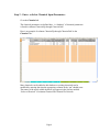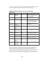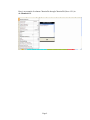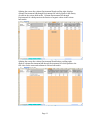
1
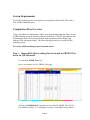
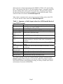
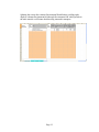
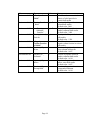
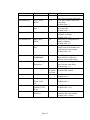
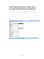
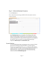
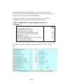
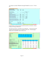
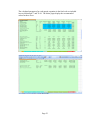
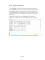
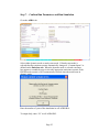
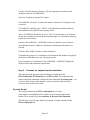
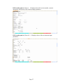
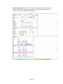
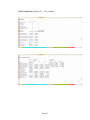
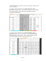
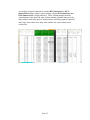
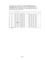
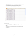
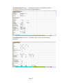
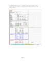
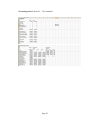
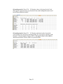
User’s Guide for CEMC_SFU_AGRO
v1.2
The Combined Canadian Environmental
Modelling Centre Water Quality Model and the
Simon Fraser University Food Web Model
Version 1.2
September 18, 2007
TABLE OF CONTENTS
Introduction........................................................................... 3
System Requirements............................................................. 4
Computation Flow Overview.................................................. 4
Step 1 - Import Daily Mass Loading Data Generated by PRZM3.12 for use in the
QWASI model. ............................................................................................................... 4
Step 2 – Enter or Select Chemical Input Parameters ..................................................... 6
Step 3 – Enter or Select Environment Input Parameters............................................... 10
Step 4 – Confirm the Emissions Parameters................................................................. 17
Dynamic Emissions .................................................................................................. 17
Constant Emissions................................................................................................... 18
Step 5 – Review the FWModel tab ............................................................................... 19
Step 6 – Review the Foodweb tab................................................................................. 24
Step 7 – Confirm Run Parameters and Run Simulation .............................................. 25
Step 8 – Examine the output from the simulation........................................................ 26
Dynamic Results ....................................................................................................... 26
Steady-state Results .................................................................................................. 35
References ........................................................................... 40
TABLES
Table 1: Summary of daily input values for AGRO model derived from PRZM
output………………………………………………………………………………… 5
Table 2: Chemical Parameters for Type I Partitioning Simulations……………. 7
Table 3: Chemical Parameters for Type I Partitioning Simulations……………. 8
Table 4: Input Parameters in the Environment Tab……………………………. 13-15
Table 5: Additional Environmental Input parameters in FWModel…………… 20
Table 6: Summary of timeseries output parameters included with the model…34
Page 2
Introduction
The Canadian Environmental Modelling Centre’s AGRO modeling system (AGRO) is a
MicroSoft Excel® based application that combines a water quality model with a food
web model to estimate risk to aquatic species from pesticide exposure in a user-defined
water body. A major feature of this system is its capability to incorporate dynamic
functionalities which allow the user to introduce changing environmental and emission
conditions so that the fate and bioaccumulation results of numerous chemicals can easily
and efficiently be compared.
The AGRO modeling system is written in Visual Basic and has an EXCEL® interface for
parameter input and output display. This system can be run in dynamic mode which uses
daily input of water, sediment, and pesticide from predicted daily mass loadings
generated by US EPA Pesticide Root Zone Model, version 3.12 (PRZM3.12) (Suárez,
2006). [Note: AGRO can also be run in a steady-state mode]. Daily loading and
emission values from PRZM3.12 are then used to generate predicted daily pesticide
concentrations in the water column, benthic pore water and benthic sediment of the water
body. From these concentrations, the food web model estimates bioaccumulation of
pesticide in aquatic organisms.
The water quality model component of the AGRO modeling system is the Quantitative
Water, Air, Sediment Interaction (QWASI) Fugacity model developed by Mackay et al.
at the Canadian Environmental Modelling Centre (Mackay, Joy and Paterson (1983),
Mackay, Paterson and Joy (1983), Mackay and Diamond (1989), Webster, Lian and
Mackay (2005)). The QWASI model is based on a single receiving water body of userdefined size and depth with an active sediment layer. This model can be run in dynamic
mode which involves daily input of water from field runoff, dissolved pesticide in field
runoff, eroded sediment, pesticide sorbed to eroded sediment, pesticide emissions
resulting from application drift and rainfall. These dynamic daily inputs are generated
outside of the AGRO modeling system using the EPA PRZM3.12. The AGRO modeling
system has built-in capability to import annual mass loading files output from PRZM3.12
and convert these values into the units and configurations needed by the QWASI
Fugacity model.
The food web model in AGRO is based on the Bioaccumulation model developed by
Frank A.P.C. at Simon Fraser University (Gobas, 2007). The Bioaccumulation model is a
dynamic or time dependent interpretation of Arnot and Gobas [2004] bioaccumulation
equation. This model is based on the assumption that the exchange of hydrophobic
organic chemicals between the organism and its ambient environment can be described
by a single equation for a large number of aquatic organisms. For each aquatic organism,
this equation estimates bioaccumulation as a function of intake of pesticide via
respiration and ingestion of prey, and outflow of pesticide via excretion, metabolism to a
daughter product and respiratory exhalation.
Page 3
System Requirements
The AGRO modeling system is designed to run using MicroSoft Excel® 2003 with at
least 10 MB of hard disk space.
Computation Flow Overview
Using Visual Basic for Applications (VBA) as the programming language allows for the
AGRO modeling system to function within the framework of EXCEL spreadsheets, thus
facilitating the entry and viewing of both the input parameters and the display and
analysis of the subsequent output. The following steps detail how to run the AGRO
modeling system.
To run the AGRO modeling system in dynamic mode:
Step 1 - Import Daily Mass Loading Data Generated by PRZM3.12 for
use in the QWASI model.
Go to the Get_PRZM_Files Tab
Here is an example of a Get_PRZM_Files page:
Click the “Get PRZM data” button located on cells Get_PRZM_Files!G(1:2)Get_PRZM_Files!H(1:2). Clicking this executes a Visual Basic macro which
Page 4
allows the user to choose the location of the PRZM3.12 P2E-c1.D* mass loading
files. Click on any of the P2E-C1.D* files and then “Open” to begin the import of
the mass loading values and to store them in this tab. This macro also converts
the data into the units and variables compatible with the QWASI model. These
converted values are stored in the PRZMforInput tab.
Table 1 below summarizes the conversion of massing loading values in the P2EC1.D* files into the values stored in the PRZMforInput tab.
Table 1: Summary of daily input values for AGRO model derived
from PRZM output
Parameter
Simday
Year Month Day
E to Pond kg/y
Inflow-W Conc
ng/L
Inflow-P Conc
ng/L
Bulk Inflow Conc
ng/L
Description
assigned to evaluate and loop through the total number of
days of data provided by PRZM
from PRZM
this is the 5% spray drift from PRZM expressed as kg/y
from PRZM expressed in ng/L
from PRZM expressed in ng/L
uses Inflow-W Conc and Inflow-P Conc with the respective
volume fractions to calculate a bulk water concentration of
chemical
Water Inflow rate Standard rate defined on Environment worksheet + PRZM
runoff
m3/h
Particulate Inflow Standard rate derived from Environment worksheet +PRZM
erosion rate
rate m3/h
derived Inflow and Particulate inflow rates
Inflow-P
concentration
Volume Fraction of water in the inflow
VF-W Inflow
Volume Fraction of particulate in the inflow
VF-P Inflow
3
converted from cm/day in PRZM to m3/h
rain rate m /h
The AGRO modeling system also contains a blank worksheet with tab entitled,
PRZM-workarea. This worksheet is used by the AGRO Visual Basic module to
store internal variable values during processing. It is always cleared at the end of
each instance of retrieval of PRZM files.
Page 5
Step 2 – Enter or Select Chemical Input Parameters
Go to the Chemical tab
The chemical parameters are defined here. A “database” of chemical parameters
is listed in columns Chemical!Q through Chemical!AK.
Here is an example of columns Chemical!Q through Chemical!AK in the
Chemical Tab:
More chemicals can be added to this database or existing chemicals can be
modified by entering data into the appropriate columns in the “tan” shaded areas.
The names of the newly added chemicals will appear in the list-box entitled
“Select a Chemical” in columns Chemical!D-Chemical!F of this tab.
Page 6
To enter a new chemical with Type I partitioning into the chemical database, enter
the following chemical information into the first available empty row:
Table 2: Chemical Parameters for Type I Partitioning
Simulations
Column
Chemical!Q
Parameter
Chemical
Identifier
Chemical!R
Chemical
--Name
Chemical Type ---
Chemical!S
Chemical!T
Chemical!U
Chemical!V
Chemical!W
Property
Temperature
Chemical
Molecular
Mass
Chemical
Melting Point
°
Solubility
Units
---
Notes
The row number plus 1. This
will be used as the chemical
number identifier.
Name of chemical of interest
°C
1 for Type I partitioning and 2
for Type II partitioning. For
regulatory modeling, Type I
partitioning is employed.
Default 17°C
g/mol
Molecular weight of chemical
°C
g/m3
Water solubility of chemical.
Equivalent units are kg/L.
Chemical!X
Chemical
Pa
Vapor Pressure
Chemical!Z
Log KOW
(mg/L)/(mg/L) Log 10 of the Octanol-Water
Partition Coefficient, KOW
Chemical!AD Chemical
days
Aqueous aerobic half-life
Half-life in
Water
Chemical!AE Chemical
days
Aqueous anaerobic half-life
Half-life in
Sediment
For Type I chemicals, Columns Chemical!AG-Chemical!AK are left blank. For
Type II chemicals (those with little or no volatility) only the Molar Mass,
Property Temperature, Degradation Half-lives and partition coefficients defined
in Chemical!AG:Chemical!AK (with appropriate units) are used. Please see
Mackay (2001) for more information on modelling Type I and Type II chemicals.
Page 7
Table 3: Chemical Parameters for Type I Partitioning
Simulations
Column
Chemical!Q
Parameter
Chemical
Identifier
Units
---
Notes
The row number plus 1. This
will be used as the chemical
number identifier.
Name of chemical of interest
Chemical!R
Chemical!S
Chemical
--Name
Chemical Type ---
Chemical!T
Property
Temperature
Chemical!U
Chemical
Molecular
Mass
Chemical!AD Chemical
Half-life in
Water
Chemical!AE Chemical
Half-life in
Sediment
Chemical!AG Air/Water
Partition
Coefficient,
KAW
Chemical!AH AerosolWater
°C
1 for Type I partitioning and 2
for Type II partitioning.
Default 17°C
g/mol
Molecular weight of chemical
days
Aqueous aerobic half-life
days
Aqueous anaerobic half-life
Chemical!AI
SedimentWater
L/kg
Chemical!AJ
Suspended
Sediment-Water
L/kg
dimensionless
dimensionless
KQW
Chemical!AK Resuspended
L/kg
Sediment-Water
Now, go to the list-box “Select a Chemical” in columns Chemical!D-Chemical!F.
Highlight the chemical of interest and click the “OK” button. This will cause the
appropriate values of the selected chemical to appear in column Chemical!B
where the user can easily review them and where the model actually reads the
values used in the upcoming simulation. (If the user wishes to make temporary
changes to a chemical data, these can be made directly in column Chemical!B
without affecting the original values in the database, although these value will be
overwritten each time the “OK” button is clicked)
Page 8
Here is an example of columns Chemical!A through Chemical!N (Rows 1-21) in
the Chemical tab:
Page 9
Step 3 – Enter or Select Environment Input Parameters
Go to the Environment tab
The environment scenario parameters are defined here. A “database” of
environmental scenarios is listed in columns Environment!O through
Environment!AW. The environmental parameters listed here are those required
to run the QWASI 3.10 model.
The user may add environmental scenarios to this database by entering necessary
information into the columns Environment!O through Environment!AW. The
names of the newly added environments will appear in the list-box entitled
“Select an Environment” in this tab.
Here is an example of columns Chemical!O through Chemical!AA of the
environmental database in the Environment tab. Columns Environment!S
through Environment!V refer to dimensions of the water body. Columns
Environment!W through Environment!AA refer to the concentration of particle
solids in the various bulk media. The “tan” cells indicate that the user may input
data in these cells.
Page 10
Splitting the screen after column Environment!R and scrolling right, displays
columns Environment!AB through Environment!AE which pertain to the density
of solids in the various bulk media. Columns Environment!AF through
Environment!AJ which pertain to the fraction of organic carbon in the various
bulk media.
Splitting the screen after column Environment!R and further scrolling right,
displays columns Environment!AK through Environment!AP which pertain to the
flow rates for the water and sediment in various bulk media.
Page 11
Splitting the screen after column Environment!R and further scrolling right,
displays columns Environment!AQ through Environment!AW which pertain to
the mass transfer coefficients characterizing intermedia transport .
Page 12
Here is a summary of the input Parameters in the Environment Tab:
Table 4: Input Parameters in the Environment Tab
Note: Default values for EPA generic pond scenario are listed in notes column.
Column
Environment!O
Parameter
“Dimensions”
Units
---
Environment!P
Selected
Environment
Identifier
---
Environment!Q
---
Environment!U
Environmental
Properties
Scenario
Identifier
Name of
Environmental
Scenario
Water_Surface_
Area
Water_Volume
m3
Environment!V
Sediment
m
Environment!W
“Concentration
of Solids”
---
Environment!X
Aerosol_Particles
ug/m3
Environment!Y
Particles_Inflow
mg/L
Environment!Z
Particles_Water_
Column
mg/L
Environment!AA
Volume_Fraction
_Particles_
Surface
m3/m3
Environment!R
Environment!T
Page 13
Notes
Label for columns associated with
dimensions of the water body
Numeric identifier of
environmental scenario
highlighted in the “Select an
Environment” list-box.
Automatically changes with
change in highlighted selection.
User-supplied numeric identifier
of environmental scenario of
interest
---
Name given to the environmental
scenario
m2
Surface area of water body
Default value: 10,000
Volume of water body
Default value: 20,000
Depth of sediment in benthic
layer.
Default value: 0.05
Label for columns associated with
concentration of solid particles in
various bulk media
Concentration of solid particles in
air bulk media.
Default value: 30
Concentration of solid particles in
inflow water bulk media.
Default Value: 2
Concentration of suspended
sediment in water column.
Default value: 30
Volume fraction of sediment
particles in benthic.
Default value: 0.5
Column
Environment!AB
Parameter
“Density of
Solids”
Units
Environment!AC
Density_Particles
_Water
kg/m3
Environment!AD
Density_
kg/m3
Sediment_
Particles
Density_Aerosol_ kg/m3
Particles
Environment!AE
Environment!AF
Environment!AG
“Organic
Carbon Fraction
of Solids"
Fraction_OC_
Water
---
Environment!AH
Fraction_OC_
Sediment
---
Environment!AI
Fraction_OC_
Inflow
---
Environment!AJ
Fraction_OC_
Resuspended
---
Page 14
Notes
Label for columns associated with
density of solid particles in
various bulk media
Density of solid particles in water
column bulk media.
Default value: 2400
Density of solid particles in
benthic sediment bulk media.
Default value: 2400
Density of solids particles in air
bulk media.
Default value: 1500
Label for columns associated with
organic carbon fraction in various
bulk media
Fraction of organic carbon in
water column bulk media.
Default value: 0.067
Fraction of organic carbon in
benthic sediment bulk media
Default value: 0.014
Fraction of organic carbon in
inflow water bulk media
Default value: 0.067
Fraction of organic carbon in
resuspended sediment.
Default value: 0.014
Column
Environment!AK
Parameter
“Flows”
Units
Environment!AL
River_Water_
Inflow
m3/h
Environment!AM
Water_Outflow_
Rate
m3/h
Environment!AN
Deposition_Rate
g/m2
Environment!AO
Burial_Rate_
Solids
g/m2
Environment!AP
Resuspension_
Rate
g/m2
Environment!AQ
Label for columns associated with
Mass transfer Coefficients
between various bulk media
Aerosol_Dry_
m/h
Deposition rate of dry particles
Deposition
out of air into water body.
Default value: 10
Scavenging_Ratio Volume of Scavenging Ratio of air to rain
air/Volum Default value: 20,000
e of Rain
Rain_Rate
m/year
Rainfall rate in meters per year.
Default value: 1
Vol_Mass_
m/h
Volatilization rate – air side
Trans_Coeff_
Default value: 1
Air
Vol_Mass_
m/h
Volatilization rate – water to air
Transfer_Coeff_
Default value: 0.01
Water
Sediment-Water- m/h
Diffusion rate between benthic
Diffusion
sediment and water column.
Default value: 0.0004
Environment!AR
Environment!AS
Environment!AT
Environment!AU
Environment!AV
Environment!AW
“Mass Transfer
Coefficients”
Page 15
Notes
Label for columns associated with
flow rates in various bulk media
Flow rate of inflow water into
water body.
Default value: 5
Flow rate of outflow water out of
the water body.
Default value: 5
Deposition rate of solid particles
to benthic sediment.
Default value: 80
Burial rate of solid particles in
benthic sediment.
Default value: 40
Resuspension rate of solid
particles out of the benthic and
back into the water column.
Default value: 40
Now, go to the list-box “Select an Environment” in columns Environment!EChemical!G. Highlight the environment of interest and click the “OK” button.
This will cause the appropriate values of the selected environment to appear in
column Environment!B where the user can easily review them and where the
model actually reads the values used in the upcoming simulation. (If the user
wishes to make temporary changes to a chemical data, these can be made directly
in column Environment!B without affecting the original values in the database,
although these value will be overwritten each time the “OK” button is clicked)
Here is an example of columns Environment!A through Chemical!N (Rows 1-33)
in the Environment tab:
Page 16
Step 4 – Confirm the Emissions Parameters
Go to the Emissions tab
Here is what the Emissions tab page should look like when dynamic emission
scenario is selected:
On the Emissions tab, there are two options. By clicking on either radio
button under the heading “Emission Type” the user may choose one of two
scenarios. The first option is used for steady-state calculations or for dynamic
ones requiring that there be constant emission of chemical over the duration of
the model run. The second option is to use the PRZM-defined inputs
imported to PRZMforInput and GetPRZMFiles tabs.
Dynamic Emissions
To use the PRZM-defined inputs and parameters, make sure that the “Defined
daily emissions (kg/Ha/day), input from PRZM” is selected so that the
Emission Type in cell Emissions!P2 is set to 2. Cell Emissions!B2 should say
“ Dynamic from PRZM” and the cells Emissions!A8:Emissions!E12 appear as
though “grayed-out”. The above set-up with “Defined daily emissions”
selected activates the dynamic mode execution of the model where daily
values are read from the PRZMforInput tab.
Page 17
The internal model code automatically navigates through the PRZMforInput
daily values until it reaches the first non-zero emissions occurrence in
PRZMforInput!E column at which time the model iterations begin.
Constant Emissions
If the “Constant Emission, average annual emission (kg/Ha/yr), input below”
radio button is selected, the cells Emissions!A8:Emissions!E12 appear with a
white background, except cells Emissions!B8, B11 and B12 which are “tan”
in colour, indicating that they are user defined inputs. The model reads in the
value for calculated direct inputs from spray drift to the pond from cell
Emissions!B9. Note that the value of 5% of the application rate to 1 Ha is
used to estimate the net input of chemical to the pond from all inputs. This is
based on the US-EPA EXAMS model treatment of spray drift inputs to an
agricultural pond.
The user may choose to enter any ambient air concentration of chemical in
Emissions!B11 or inflow water concentration. Inflow water can be in the
form of inflow derived from any source (inflow from another body of water,
from groundwater or from runoff water), as long as the corresponding flow for
this concentration is quantified on the Environment worksheet. The net
annual input of chemical to the pond is derived using:
Conc inflow ng/L * kg/1x1012 ng * 1000 L/m3 * Inflow rate m3/h * 8760 h/yr
The result (kg/yr) inflow of chemical is added to the kg/yr estimate of direct
emission to the pond via spray drift for a total chemical input rate.
Page 18
Step 5 – Review the FWModel tab
Go to the FWModel tab. This tab contains the chemical and ecosystem
parameter values used by the Gobas Bioaccumulation model. Review the
assigned input values.
Usually, the user will not make any revisions to this tab since the Environmental
Fate Parameters on this worksheet are mostly calculated based on values entered
in the Environment and Chemical tabs and the Food Web Bioaccumulation
Model values are the recommended values for the embedded organism foodweb.
Note: There is no database summarizing several possible foodwebs, so any
changes made are permanent and it is suggested that an original version of
the file be maintained at all times to preserve the original information.
Columns FWModel!A through FWModel!G summarize the Chemical and
Environmental Fate input parameters from the QWASI water quality model.
For columns FWModel!A through FWModel!G, rows 4 – 10, the chemical
parameters required by the Bioaccumulation model are automatically summarized
based on input values entered in the Chemical tab.
An example of columns FWModel!A through FWModel!G, rows 4 – 10 looks
like:
Page 19
For columns FWModel!A through FWModel!G, rows 12 – 31, the chemical
parameters required by the Bioaccumulation model are automatically summarized
based on input values entered in the Environment tab.
The following additional environmental input parameters along with their
recommended values are required by the Bioaccumulation model:
Table 5: Additional Environmental Input parameters in
FWModel
Input Parameter
Dissolved oxygen saturation (%)
Disequilibrium factor POC (unitless)
Disequilibrium factor DOC (unitless)
POC-octanol proportionality constant (unitless)
DOC-octanol proportionality constant (unitless)
pH of water
water temperature (degC)
Sediment OC octanol proportionality constant (unitless)
initial chemical mass in water (g)
initial chemical mass in sediment (g)
Recommended
Value
90%
1
1
0.35
0.08
7
17
0.35
0
0
An example of columns FWModel!A through FWModel!G, rows 4 – 10 looks
like:
Page 20
An example of columns FWModel!A through FWModel!G, rows 41 – 65 looks
like:
An example of columns FWModel!A through FWModel!G, rows 66 – 87 looks
like:
Page 21
An example of columns FWModel!A through FWModel!G, rows 66 – 87 looks
like:
Food Web input values for the Bioaccumulation model are included in columns
FWModel!G through FWModel!L.
The food web structure is included in rows 5 through 13. . The food web aquatic
organism individual parameters are included in rows 18-38. The below page
displays the recommended values for these rows:
Page 22
The calculated parameters for each aquatic organism in the food web are included
in rows 40 through 77 and 79-89. The below pages display the recommended
values for these rows:
Page 23
Step 6 – Review the Foodweb tab
Go to the Foodweb tab. All values in this tab are automatically summarized
from the FWModel tab. Thus, the user will never make any revisions to this tab.
The Foodweb tab summarizes the calculated k-values and the Feeding Matrix
from the FWModel tab. The Foodweb tab is where the Bioaccumulation model
actually reads in its input values to populate the foodweb and generate organism
concentrations.
The page below displays a copy of the Foodweb tab with recommended
calculated masses, lipid fractions, k-rates, and feeding matrix for the food web.
Page 24
Step 7 – Confirm Run Parameters and Run Simulation
Go to the AGRO tab
Select either dynamic mode or steady-state mode. If Steady-state mode is
selected then the emission scenario automatically changes to “Constant Inputs” as
defined on the Emissions tab. When the dynamic mode is selected a message
box appears to remind the user to select the appropriate emissions scenario as the
PRZM-based scenario is NOT automatically selected when the model runs in
dynamic mode.
Enter the number of years of the simulation in cell AGRO!B14.
To output daily, enter “24” in cell AGRO!B15.
Page 25
Use the “calculate timestep” button to fill in the appropriate timestep for the
modelled system in cell AGRO!B16.
Select the “Outputs in separate file” option.
Cell AGRO!P2 will read 1 if steady-state mode is selected or 2 if dynamic mode
is selected.
Cell AGRO!P3 should be set to “TRUE” so that the Bioaccumulation model is
run in addition to the QWASI water quality model.
Also, cell AGRO!P4 should also be set to “True” so the timestep set as constant
for the entire simulation, otherwise the model attempts to recalculate the timestep
required at each iteration.
Examine cells AGRO!B4 – AGRO!B8 to make sure that the correct chemical,
environmental scenario, foodweb, and dynamic simulation model options are
selected.
Click the “Run AGRO” button to run the simulation.
To monitor the progress of a simulation, each simulation day number is displayed
on the lower left-hand corner as it is being processed.
Upon completion of a simulation, Cells AGRO!B24 – AGRO!B33 display the
model run time and simulation mass balance.
Step 8 – Examine the output from the simulation
The output from the dynamic mode simulation is displayed in tabs
DYN-results-pond, DYN-timeseries, and DYN-yearly. The output from the
steady-state mode simulation is displayed in the tab named SS-results-pond. An
overview of the format of the dynamic results is presented, followed by an
overview of the steady-state results.
Dynamic Results
The results presented in the DYN-results-pond tab are in the
same format as the QWASI model with the foodweb results output at the
bottom. These results reflect the conditions at the end of the simulation.
The following series of pages display an example of output contained in the
DYN-results-pond tab.
Page 26
DYN-results-pond tab, Rows 1 - 43 display the model version number, scenario
descriptors, and echoes of the chemical input parameters.
DYN-results-pond tab, Rows 44 - 91 display echoes of the environment input
parameters.
Page 27
DYN-results-pond tab, Rows 92 - 228 display results from the QWASI water
quality model. These include mass balances over the simulated time for the
chemical in both water and benthic sediment.
Page 28
DYN-results-pond tab, Rows 92 - 228, continued.
Page 29
DYN-results-pond tab, Rows 229 - 250 display echoes of the input for the Food
Web aquatic organism masses, lip fraction, k-rates and feeding table matrix used
by the Bioaccumulation model.
DYN-results-pond tab, Rows 251 - 263 display calculated results of pesticide
concentrations from the Bioaccumulation model for each aquatic organism in the
food web. The organism Biomagnificaton Factors (BMFs) and the Theoretical
Maximum BMFs (calculated by kd/ke) are presented.
Page 30
The DYN-timeseries tab contains the values of selected output variables for each
day of the simulation.
An example of output contained in columns DYN-timeseries!A - DYNtimeseries!P is displayed below. These columns summarize the daily simulation
date, emission, fugacities for each bulk media, and bulk media chemical
concentrations in natural units.
An example of output contained in columns DYN-timeseries!A - DYNtimeseries!D and then window split to display columns DYN-timeseries!R DYN-timeseries!Z is displayed below. These columns summarize the daily
chemical concentrations for aquatic organism in the food web.
Page 31
An example of output contained in columns DYN-timeseries!A - DYNtimeseries!D and then window split to display columns DYN-timeseries!AA DYN-timeseries!AJ is displayed below. These columns display the daily
concentrations in the dissolved water column, benthic sediment and pore water
along with the total daily input of chemical mass, total daily output of chemical
mass, daily water inflow rate, daily water outflow rate, and net daily water
volume flux.
Page 32
An example of output contained in columns DYN-timeseries!A - DYNtimeseries!D and then window split to display columns DYN-timeseries!AL DYN-timeseries!AX is displayed below. These columns display the particle
solid fluxes in the water column and benthic sediment along with various water
and sediment daily fluxes in mol basis.
Page 33
The following table summarizes the columns in the columns of the DYNtimeseries tab:
Table 6: Summary of timeseries output parameters included with
the model
Variable/Parameter
Time (h)
Year
Month
Day
Emission kg/year
Fugacity, Pa
Water
Sediment
Inflow
Air
Pure Phase Chemical
Bulk Concentrations (natural units)
Water, ng/L
Sediment, ng/m3
Inflow, ng/L
Air, ug/m3
Foodweb Concentrations, ng/g
Water-dissolved only, ug/L
Sediment-solids only
Phytoplankton
Zooplankton
Benthic Invertebrates
Forage Fish A
Forage Fish B
Piscivorous Fish
Other
SumInput kg
SumLoss kg
Water inflow m3/h
Water outflow m3/h
Net water m3/h
Sed Inflow m3/h
Sed Resusp m3/h
Sed outflow m3/h
Sed Dep m3/h
Net Sed m3/h
Page 34
Description (if necessary)
From PRZM3.12
From PRZM3.12
From PRZM3.12
(if it occurs at this output interval)
Cumulative system Input of chemical
Cumulative system Loss of chemical
Inflow-Outflow
Inflow + Resusp – Outflow – Dep
The DYN-yearly tab contains the Estimated Environmental Concentrations
(EECs) for the peak, 4-day, 21-day, 60-day, 90-day and Annual running averages
for the chemical dissolved water column (for the highest 4 years of the
simulation), benthic sediment sorbed chemical (for the highest 4 years of the
simulation), and chemical dissolved in benthic pore water (for all years).
Steady-state Results
The results presented in the SS-results-pond tab are in the
same format as the QWASI model with the foodweb results output at the
bottom.
The following series of pages display an example of output contained in the SSresults-pond tab.
Page 35
SS-results-pond tab, Rows 1 - 44 display the model version number, scenario
descriptors, and echoes of the chemical input parameters.
SS-results-pond tab, Rows 44 - 88 display echoes of the environment input
parameters.
Page 36
SS-results-pond tab, Rows 92 - 228 display results from the QWASI water
quality model. These include mass balances for the chemical in both water and
benthic sediment.
Page 37
SS-results-pond tab, Rows 92 - 228, continued.
Page 38
SS-results-pond tab, Rows 230 - 250 display echoes of the input for the Food
Web aquatic organism masses, lip fraction, k-rates and feeding table matrix used
by the Bioaccumulation model.
SS-results-pond tab, Rows 251 - 263 display calculated results of pesticide
concentrations from the Bioaccumulation model for each aquatic organism in the
food web. Bioconcentration Factors (BCFs), Biomagnification Factors (BMFs)
and Bioaccumulation Factors (BAFs) are presented here.
Page 39
References
Alpine AE, Cloern JE. 1988. Phytoplankton Growth Rates in a Light-Limited
Environment, San Francisco Bay. Marine Ecology - Progress Series 44: 167173.
Alpine AE, Cloern JE. 1992. Trophic Interactions and Direct Physical Effects
Control Phytoplankton Biomass and Production in an Estuary. Limnology and
Oceanography 37(5): 946-955.
Arnot JA, Gobas FAPC. 2004. A Food Web Bioaccumulation Model for Organic
Chemicals in Aquatic Ecosystems. Environmental Toxicology and Chemistry
23(10): 2343-2355.
Berg DJ, Fisher SW, Landrum PF. 1996. Clearance and Processing of Algal
Particles by Zebra Mussels (Dreissena polymorpha). Journal of Great Lakes
Research 22: 779-788.
Branson DR, Blau GE, et al. 1975. Bioconcentration of 2,2,4,4-Tetrachlorobiphenyl
in Rainbow Trout as Measured by an Accelerated Test. Transactions of the
American Fisheries Society 104: 785-792.
Bruner KA, Fisher SW, Landrum PF. 1994. The Role of the Zebra Mussel,
Dreissena polymorpha, in Contaminant Cylcing: II. Zebra Mussel
Contaminant Accumulation from Algae and Suspended Particles and Transfer
to the Benthic Invertebrate, Gammarus fasciatus. Journal of Great Lakes
Research 20: 735-750.
Burkhard LP. 2000. Estimating Dissolved Organic Carbon Partition Coefficients for
Nonionic Organic Chemicals. Environmental Science and Technology 34:
4663-4668.
Ernst W, Goerke H. 1976. Residues of Chlorinated Hydrocarbons in Marine
Organisms in Relation to Size and Ecological Parameters. I. PCB, DDT, DDE
and DDD in Fishes and Molluscs from the English Channel. Bulletin of
Environmental Contamination and Toxicology 15: 55-65.
Fisk AT, Norstrom RJ, et al. 1998. Dietary Accumulation and Depuration of
Hydrophobic Organochlorines: Bioaccumulation Parameters and their
Relationship with the Octanol/Water Partition Coefficient. Environmental
Toxicology and Chemistry17: 951-961.
Gobas FAPC. 1993. A Model for Predicting the Bioaccumulation of Hydrophobic
Page 40
Organic Chemicals in Aquatic Food webs: Application to Lake Ontario.
Ecological Modelling 69: 1-17.
Gobas FAPC, Mackay D. 1987. Dynamics of Hydrophobic Organic Chemical
Bioconcentration in Fish. Environmental Toxicology and Chemistry 6: 495504.
Gobas FAPC, Muir DCG, Mackay D. 1988. Dynamics of Dietary Bioaccumulation
and Faecal Elimination of Hydrophobic Organic Chemicals in Fish.
Chemosphere 17: 943-962.
Gobas FAPC, McCorquodale JR, Haffner GD. 1993a. Intestinal Absorption and
Biomagnification of Organochlorines. Environmental Toxicology and
Chemistry 12: 567-576.
Gobas FAPC, Zhang X, Wells R. 1993b. Gastrointestinal Magnification: The
Mechanism of Biomagnification and Food Chain Accumulation of Organic
Chemicals. Environmental Science and Technology 27: 2855-2863.
Gobas FAPC, Wilcockson J, et al. 1999. Mechanism of Biomagnification in Fish
under Laboratory and Field Conditions. Environmental Science and
Technology 33: 133-141.
Gobas FAPC, Maclean LG. 2003. Sediment-Water Distribution of Organic
Contaminants in Aquatic Ecosystems: The Role of Organic Carbon
Mineralization. Environmental Science and Technology 37: 735-741.
Gordon DCJ. 1966. The Effects of the Deposit Feeding Polychaete Pectinaria
gouldii on the Intertidal Sediments of Barnstable harbor. Limnology and
Oceanography 11: 327-332.
Koelmans AA, Anzion SFM, Lijklema L. 1995. Dynamics of Organic
Micropollutant Biosorption to Cyanobacteria and Detritus. Environmental
Science and Technology 29: 933-940.
Koelmans AA, Jiminez CJ, Lijklema L. 1993. Sorption of Chlorobenzenes to
Mineralizing Phytoplankton. Environmental Toxicology and Chemistry 12:
1425-1439.
Koelmans AA, van der Woude H, et al. 1999. Long-term Bioconcentration Kinetics
of Hydrophobic Chemicals in Selensatrum capricornutum and Microcystis
aeruginosa. Environmental Toxicology and Chemistry 18: 1164-1172.
Kraaij R, Seinen W, et al. 2002. Direct Evidence of Sequestration in Sediments
Affecting the Bioavailability of Hydrophobic Organic Chemicals to Benthic
Deposit-Feeders. Environmental Science and Technology 36: 3525-3529.
Page 41
Kukkonen J, Landrum PF. 1995. Measuring Assimilation Efficiencies for
Sediment-Bound PAH and PCB Congeners by Benthic Invertebrates. Aquatic
Toxicology 32: 75-92.
Landrum PF, Poore R. 1988. Toxicokinetics of Selected Xenobiotics in Hexagenia
limbata. Journal of Great Lakes Research 14: 427-437.
Lehman JT. 1993. Efficiencies of Ingestion and Assimilation by an Invertebrate
Predator using C and P Dual Isotope Labeling. Limnology and Oceanography
38: 1550-1554.
Lydy MJ, Landrum PF. 1993. Assimilation Efficiency for Sediment Sorbed
Benzo(a)pyrene by Diporeia spp. Aquatic Toxicology 26: 209-224.
Mackay, D. 2001. "Multimedia Environmental Models: The Fugacity Approach Second edition", Lewis Publishers, Boca Raton. pp. 201-213.
Mackay, D., Diamond, M. 1989. Application of the QWASI (Quantitative Water
Air Sediment Interaction) Fugacity Model to the Dynamics of Organic and
Inorganic Chemicals in Lakes. Chemosphere. 18: 1343-1365.
Mackay, D., Joy, M., Paterson, S. 1983. A Quantitative Water, Air, Sediment
Interaction (QWASI) Fugacity Model for Describing The Fate of Chemicals in
Lakes. Chemosphere. 12: 981-997.
Mackay, D., Paterson, S., Joy, M. 1983. A Quantitative Water, Air,
Sediment Interaction (QWASI) Fugacity Model for Describing the Fate of
Chemicals in Rivers. Chemosphere. 12: 1193-1208.
Mayer LM, Weston DP, Bock MJ. 2001. Benzo(a)pyrene and Zinc Solubilization
by Digestive Fluids of Benthic Invertebrates - A Cross-Phyletic Study.
Environmental Toxicology and Chemistry 20: 1890-1900.
McCarthy JF, Jimenez BD. 1985. Reduction in Bioavailability to Bluegills of
Polycyclic Aromatic Hydrocarbons Bound to Dissolved Humic Material.
Environmental Toxicology and Chemistry 4: 511-521.
McCarthy JF. 1983. Role of Particulate Organic Matter in Decreasing
Accumulation of Polynuclear Aromatic Hydrocarbons by Daphnia magna.
Archives of Environmental Contamination Toxicology. 12: 559-568.
Morrison HA, Gobas FAPC, et al. 1996. Development and Verification of a
Bioaccumulation Model for Organic Contaminants in Benthic Invertebrates.
Page 42
Environmental Science and Technology 30(11): 3377-3384.
Nichols JW, Fitzsimmons PN, et al. 2001. Dietary Uptake Kinetics of 2,2',5,5'Tetrachlorobiphenyl in Rainbow Trout. Drug Metabolism and Disposition 29:
1013-1022.
Oliver, B. G. and A. J. Niimi 1988. Trophodynamic Analysis of Polychlorinated
Biphenyl Congeners and Other Chlorinated Hydrocarbons in the Lake Ontario
Ecosystem. Environmental Science and Technology 22: 388-397.
Parkerton TF. 1993. Estimating Toxicokinetic Parameters for Modelling the
Bioaccumulation of Non-Ionic Organic Chemicals in Aquatic Organisms.
PhD thesis. Rutgers The State University of New Jersey, New Brunswick, NJ,
USA.
Payne SA, Johnson BA, Otto RS. 1999. Proximate Composition of some NorthEastern Pacific Forage Fish Species. Fish Oceanography 8: 159-177.
Reid, L. 2007 pers. comm. “AGRO-BASF Model Version 1.16” Excel workbook and
Visual Basic model code, Canadian Environmental Modelling Centre, Trent University,
Peterborough, Ontario, K9J 7B8, Canada. http://www.trentu.ca/cemc/
Roditi HA, Fisher NS. 1999. Rates and Routes of Trace Element Uptake in Zebra
Mussels. Limnology and Oceanography 44: 1730-1749.
Rosen DAS, Williams L, et al. 2000. Effect of Ration Size and Meal Frequency on
Assimilation and Digestive Efficiency in Yearling Stellar Sea Lions,
Eumetopias jubatus. Aquatic Mammals 26: 76-82.
Russell RW, Gobas FAPC, Haffner GD. 1999. Maternal Transfer and In-Ovo
Exposure of Organochlorines in Oviparous Organisms: A Model and Field
Verification. Environ. Sci. Technol. 33: 416-420.
Seth R, Mackay D, Muncke J. 1999. Estimating the Organic Carbon Partition
Coefficient and its Variability for Hydrophobic Chemicals. Environmental
Science and Technology 33: 2390-2394.
Skoglund RS, Swackhamer DL. 1999. Evidence for the Use of Organic Carbon as
the Sorbing Matrix in the Modeling of PCB Accumulation in Phytoplankton.
Environmental Science and Technology 33: 1516-1519.
Suárez, L.A., 2006. PRZM-3, A Model for Predicting Pesticide and Nitrogen
Fate in the Crop Root and Unsaturated Soil Zones: Users Manual for Release 3.12.2.
National Exposure Research Laboratory,U.S. Environmental Protection Agency Athens,
GA 30605-2700.
Page 43
Swackhamer DL, Skoglund RS. 1993. Bioaccumulation of PCBs by Algae:
Kinetics versus Equilibrium. Environmental Toxicology and Chemistry 12:
831-838.
Thomann RV. 1989. Bioaccumulation Model of Organic Chemical Distribution in
Aquatic Food Chains. Environmental Science and Technology 23: 699-707.
Thurston RV, Gehrke PC. 1990. Respiratory Oxygen Requirements of Fishes:
Description of OXYREF, a Data File Based on Test Results Reported in the
Published Literature. Proceedings of an International Symposium.,
Sacramento, California, USA, 1993.
Walker CH. 1987. Kinetic Models for Predicting Bioaccumulation of Pollutants in
Ecosystems. Environmental Pollution 44: 227-240.
Wang WX, Fisher NS. 1999. Assimilation Efficiencies of Chemical Contaminants
in Aquatic Invertebrates: A Synthesis. Environmental Toxicology and
Chemistry 18: 2034-2045.
Webster, E., Lian, L., Mackay, D. 2005. Application of the Quantitative Water Air
Sediment Interaction (QWASI) Model to the Great Lakes. Report to the Lakewide
Management Plan (LaMP) Committee CEMC Report 200501. Trent University,
Peterborough, Ontario.
Weininger D. 1978. Accumulation of PCBs by Lake Trout in Lake Michigan. PhD
thesis. University of Wisconsin, Madison, WI, USA.
Xie WH, Shiu WY, Mackay D. 1997. A Review of the Effect of Salts on the
Solubility of Organic Compounds in Seawater. Marine Environmental
Research 44(4): 429-444.
Page 44