Download USER MANUAL - Quark Nova Project

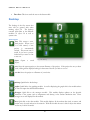
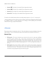
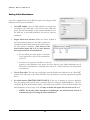
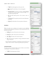
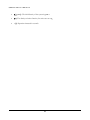
Version
2
r-JAVA 2.0
r-Process code for the Java platform
USER
MANUAL
QUARK NOVA PROJECT
r-Java 2.0 User Manual
 Quark Nova Project
University of Calgary
2500 University Dr. NW
Calgary, Alberta, Canada
T2N 1N4
http://quarknova.ucalary.ca
Table of Contents
Introduction .............................................................................. 1
Quick Start ............................................................................... 2
Graphical User Interface .......................................................... 4
Toolbar ............................................................................................ 4
Desktop ........................................................................................... 5
System Tools .................................................................................. 5
Modules .......................................................................................... 5
Commands...................................................................................... 6
Information ...................................................................................... 6
Recent projects ............................................................................... 6
Data Handling .......................................................................... 7
Adjusting Data ................................................................................. 8
Codes..................................................................................... 10
NSE............................................................................................... 11
Fission........................................................................................... 11
r-Process....................................................................................... 12
Network Type .......................................................................................... 12
Setting Initial Abundances ...................................................................... 13
Environment Type ................................................................................... 14
Graphs ................................................................................... 17
Graph Parameters .................................................................................. 17
Q U A R K
N O V A
P R O J E C T
Chapter
1
Introduction
T
he rapid capture of neutrons and subsequent beta-decay of the unstable neutron-rich isotopes or rprocess is needed to explain the origin of many heavy neutron–rich nuclei. The astrophysical site
where the r-process occurs, however, has not been positively identified. Candidate avenues of research
involve the study of winds around proto-neutron stars, ejecta from neutron star mergers and
decompressing neutron-rich matter from the surface of neutron stars. Several mechanisms may play a role in
this decompression, include the quark nova.
Code has been developed at the Quark Nova Project (QNP) to calculate the abundance of nuclei produced via
the r-process. This code is capable of investigating any of the proposed astrophysical sites and as well allows
for the study of other possible r-process environments. r-Java is a graphical user interface to this code that
makes exploring the parameter space simple and intuitive.
This manual describes the functionality of this graphical interface and assists in the use of the software. The
underlying code and methods for the r-process calculation are not described here. For an in-depth review of
the code and its application please see the following papers:
“r-Java 2.0 – the nuclear physics". Mathew Kostka, Nico Koning, Zach Shand, Rachid Ouyed and
Prashanth Jaikumar.
“r-Java 2.0 – the astrophysics". Mathew Kostka, Nico Koning, Rachid Ouyed, Prashanth Jaikumar and
Zach Shand.
These papers are available on the Quark Nova Project (QNP) website at: http://quarknova.ucalgary.ca
1
Q U A R K
N O V A
P R O J E C T
Chapter
2
Quick Start
r
-Java 2.0 was designed to be user friendly and easy to use. As such, starting and running a project
involves very few steps. This chapter will present you with a quick no-details list of commands to get
started. Once started you can explore the interface on your own or read further to understand the full
details of the software.
1. Launch r-Java 2.0 via java webstart on the QNP website.
2. Click on the “Graphs” icon near the center of the main window.
3. Click on the graph that appears in order to populate the “Graph Parameters” panel directly to the right
of the graph.
4. Click on the “X axis” tab in the “Graph Parameters” panel; change the type to “A”, set “Min:” to “0”,
“Max:” to “200” (press “Enter” after you input the values for each) and toggle “Lock” to enabled.
5. Click on the “Y axis” tab in the “Graph Parameters” panel; change the type to “Abundance”, set
“Min:” to “1e-15”, “Max:” to “1” (again remember to press “Enter” after you input the values for
each), toggle “Lock” and “Log:” to enabled.
Running
NSE
Running
r-process
6. Click on the “Code” tab in the right-most panel of the main window and choose “NSE” (Nuclear
Statistical Equilibrium) as the code type.
7. Enter the following values (remember to press “Enter” after you input the values for each): T = 3 E9,
ρ = 1E7, Ye = 0.3 and click on the “Calculator” icon in the main toolbar. The abundances will then be
calculated and displayed on the graph.
8. Select “r-Process” from the “Type:” drop-down box, located at the top of the right-most panel of the
main window.
9. Switch to the “Data” module by clicking on the
icon along the main toolbar. Click the “Restore”
button (green curved arrow) at the top of the data table. Note: It will take a few seconds to restore the
data to default values, so if you move on to the next step and the scroll bar does not respond, that is
why…just wait a couple more seconds…there it should be done now.
2
Q U A R K
N O V A
P R O J E C T
10. Scroll down in the table to “Element” = Fe, “Z” = 26, “A” = 56. In this row, under the column
“Initial MF” change the value from 0.0 to 0.3 (remember to press “Enter” after making this change).
11. In the “Code Parameter” panel, enter the following parameter values (remember to press “Enter” after
each entry): T0 = 1E9, ρ0 = 1E8, τ = 0.001, Decay time = 1E4 and Update = 50 and click on the
“Calculator” icon in the main toolbar. The abundances will then be calculated and displayed on the
graph. You can navigate between the “Messages” module (to view the evolution of the physical
parameters) and the “Graphing” module (to view the changes in the nuclei abundances) without
disturbing the code.
Running
fission
12. Select “Fission” from the “Type:” drop-down box, located at the top of the right-most panel of the
main window.
13. Click on the blue plus symbol at the bottom of the right-most panel of the main window. Select “Z:
92.0 A: 235.0” from the list shown in the pop-up window and click “OK”.
14. Click on the “Calculator” icon in the main toolbar. The fission fragmentation distribution will be
calculated and displayed on the graph.
15. To store your results for comparison with a future simulation click on the “Data” tab in the “Graph
Parameters” panel (directly to the right of the graph). Click on the words “Primary Data [Point]” in the
text field and then in the “Properties” panel that appears below change the “Name:” and “Color:”
fields. The next simulation run will regenerate a “Primary Data [Point]” data set.
16. To save the graph, right click anywhere on the graph and choose “Save Ascii” or “Save Image”
depending on if you want to save the text data, or the image respectively.
17. Save the project by clicking the “Save” icon in the main toolbar or by clicking on the “Desktop” icon
on the main toolbar (left-most icon) and then clicking on the “Save” or “Save As” icons.
18. You can then open this project at a future time by using the “Open” icon in the toolbar, or the “Open”
icon on the “Desktop” or if the project appears under “Recent projects” on the “Desktop” by clicking
on the icon with the desired project name.
The above steps should get you started in exploring the user interface. Feel free to change parameters and
options to see what the program can do.
3
Q U A R K
N O V A
P R O J E C T
Chapter
3
Graphical User Interface
r
-Java is graphical user interface to the r-process code. Navigating the toolbars, menus and graphs is
meant to be intuitive. This section will briefly cover the function of each interface component. An
important point to note is that when you enter a value in a text box, you must press “Enter” for the
change to be recorded. r-Java 2.0 does not monitor key presses and will not update unless “Enter” is
pressed. Individual modules can be detached from the main r-Java 2.0 window by clicking the
icon.
Toolbar
Desktop Calculate
Open
Save
Graphs
Elements Messages Data
Fig. 1: The toolbar.
The toolbar is always present along the top of the main window of r-Java 2.0. The toolbar provides a graphical
interface to some common commands in r-Java 2.0. The icons represent:
•
Desktop Icon: This icon sends the user to the desktop module.
•
Calculate Icon: This is the most important icon of r-Java 2.0 which starts off any abundance
calculation.
•
Open Icon: Opens a saved project.
•
Save Icon: Saves the current project.
•
Graphs Icon: This icon sends the user to the graphing module.
•
Elements Icon: This icon sends the user to the 3D periodic table module.
•
Messages Icon: This icon sends the user to the messages module.
4
Q U A R K
•
N O V A
P R O J E C T
Data Icon: This icon sends the user to the data module.
Desktop
The desktop is the first screen that
users will be greeted with when
running r-Java 2.0. The desktop
contains quick links to the different
modules of r-Java 2.0 as well as
system tools.
System Tools
•
New: This creates a new,
blank project. When r-java
2.0 is first started, a new
project is automatically
created. This menu item is
useful if you have a project
loaded and you want to start
a new one.
•
Open: Opens
project.
•
Save: Saves the current project to the current filename of the project. If the project has not yet been
saved, a dialog will be displayed asking for the name of the file you wish to save to.
•
Save As: Saves the project to a filename of your choice.
a
saved
Fig. 2: The desktop.
Modules
•
Desktop: Quick link to the desktop.
•
Graphs: Quick link to the graphing module. As well as displaying the graphs this is the module where
the user can output the calculated abundances.
•
Messages: Quick link to the messages module. This module displays updates on the physical
parameters of the system (such as temperature and density) at the current simulation time. Error
messages are as well displayed in this module.
•
Data: Quick link to the data module. This module displays all the nuclear data (such as masses and
reaction rates) for each nucleus in the network. With this module the user is able to adjust the nuclear
data for any or all of the nuclei.
5
Q U A R K
•
N O V A
P R O J E C T
Elements: Quick link to the 3D periodic table module.
Commands
•
Calculate: Begin a simulation run based on the code parameters set by the user.
Information
•
Memory: Opens a window that displays memory information such as; average memory usage, total
memory used and memory usage rate.
•
Progress: Opens window that displays the progress of the current simulation run.
•
Help: Opens the user manual.
Recent projects
In the “recent projects” section of the desktop a list of up to six (6) of the most recently used projects are
displayed for quick access.
•
Project name: Loads the r-Java 2.0 project of the given name.
6
Q U A R K
N O V A
P R O J E C T
Chapter
4
Data Handling
S
ince r –Java 2.0 calculates abundances of
nuclei, certain nuclear data, such as
neutron capture cross-sections and decay
rates, is needed before the calculations
can commence. By default r-Java 2.0 has a set of
all the necessary data loaded, see the paper “rJava 2.0 – the nuclear physics” for details on the
derivation of the data.
All of the data used by r-Java 2.0 can be viewed
in the “Data module”.
This module is
dominated by an editable table that contains all
of the data.
The user can adjust the amount of data displayed
by toggling on/off the selections listed in the
“Display” panel. Regardless of these selections
the table will always include; “Element”, “Z”
(number of protons) and “A” (atomic mass
number).
Fig. 3: The data module.
•
General Data: When selected the table will include; “Mass
[amu]” (the atomic mass of the nuclei), “Solar MF” (the solar
mass fraction of the nuclei), “Mass Fraction” (the computed
mass fraction of the nuclei for the last simulation run) and
“Initial MF” (used in the full reaction network calculation as
the initial abundance of the r-process simulation).
•
Nuclear Data: When selected the table will include; “Alpha
Decay Rate [s^-1]”, “Beta Decay Rate [s^-1]”, “Beta Decay Q
value” (the energy released by a beta decay), “Prob. 0 bdn’s” (the probability that during beta decay
zero neutrons will be emitted), “Prob. 1 bdn’s” (the probability that during beta decay one neutron will
be emitted), “Prob. 2 bdn’s” (the probability that during beta decay two neutrons will be emitted) ,
“Prob. 3 bdn’s” (the probability that during beta decay three neutrons will be emitted). The
Fig. 4: The display panel.
7
Q U A R K
N O V A
P R O J E C T
probability of beta-delayed neutron emission can be anything between 0 and 1 however r-Java 2.0 will
automatically normalize the probabilities after any change.
•
Fission Data: When selected the table will include; “Prob (BDF)” (the probability that beta decay
will lead to immediate fission of the resultant nucleus), “Fission Barrier [MeV]” and a list of
temperature dependent neutron-induced fission rates, by default there a 28 different temperature
points denoted as “nf_T0”,…,”nf_T27”. The temperature grid points are (in units of 109 K);
0.001, 0.005, 0.01, 0.05, 0.1, 0.15, 0.2, 0.25, 0.3, 0.4, 0.5, 0.6, 0.7, 0.8, 0.9, 1, 1.5, 2, 2.5, 3, 3.5, 4, 5, 6,
7, 8, 9, 10. r-Java 2.0 uses a custom interpolation technique in order to determine the intermediate
rates.
•
(n, γ)(γγ, n) Data: When selected the table will include a list of the Maxwellian-averaged neutron
capture cross sections (NA <σ ν> in units of mol-1 cm3 s-1) and (γ, n) Maxwellian-averaged photo-rates
(in units of s-1). The temperature grid points are the same as that for the neutron-induced
fission rates (in units of 109 K); 0.001, 0.005, 0.01, 0.05, 0.1, 0.15, 0.2, 0.25, 0.3, 0.4, 0.5, 0.6, 0.7,
0.8, 0.9, 1, 1.5, 2, 2.5, 3, 3.5, 4, 5, 6, 7, 8, 9, 10.
Adjusting Data
The user can change any adjustable parameter by double-clicking its cell in the table located in the Data module.
The parameters that are not adjustable are; Z, A, N, Solar Mass Fraction (MF) and Mass Fraction (this
column is where the output of the calculation is displayed). If the user is interested in adjusting a large set of
data using the table would be cumbersome and thus r-Java 2.0 provides the user with the option to change the
data as a batch.
Batch Data Adjustments
There is an option in r-Java 2.0 to simply switch between nuclear
mass models. By switching the mass model a new set of nuclei is
loaded into r-Java 2.0 with masses and associated rates calculated with
the logic of the chosen mass model.
If the user of r-Java 2.0 chooses to make custom changes to the data
we recommend that the user first exports the data set that will be
changed in order to preserve the scope of the network. Then once
the user has made changes to the data set, import the data back
into r-Java 2.0. This is recommended because typos such as making
an isotopic chain discontinuous could lead to unrealistic results from
the simulations. As well first exporting the data and then modifying
Fig. 5: Batch data adjustments.
8
Q U A R K
N O V A
P R O J E C T
the output file ensures that the format is correct when re-importing the data set.
•
Changing Temperature Dependent Rates: The neutron-induced fission cross-sections, the
neutron capture cross-sections and photorates are interpolated from a temperature grid. By default the
temperature grids have 28 points (in units of 109 K; 0.001, 0.005, 0.01, 0.05, 0.1, 0.15, 0.2, 0.25, 0.3,
0.4, 0.5, 0.6, 0.7, 0.8, 0.9, 1, 1.5, 2, 2.5, 3, 3.5, 4, 5, 6, 7, 8, 9, 10) and each nuclei has a rate (and crosssections) associated with each grid point. If the user wishes to change the range of the temperature
grid this can be done while importing a new data set. An excerpt of a (n,γ)(γ,n) data file can be seen in
Fig. 6. The series of numbers (separated by tabs) following the “T9” defines the range of the
temperature grid (in units of 109 K), the numbers must be increasing from left to right.
Fig. 6: Emaple (n,g)(g,n) data file.
For the case of the (n,γ)(γ,n) data file each row after the commented out section (comment string is #)
follows the same format; Z, A, NA<σν> @ T0, NA<σν> @ T1,…, NA<σν> @ TN, λγ @ T0, λγ @
T1,…, λγ @ TN, where T0 represents the first temperature point in the grid and TN the last
temperature point in the grid. When making changes to the (n,γγ)(γγ,n) data file the user must
ensure that there is a neutron capture cross-section and photorate associated with every
temperature grid point.
9
Q U A R K
N O V A
P R O J E C T
Chapter
5
Codes
I
sotope abundances are the main output from r-Java 2.0 calculations. There exists, however, three
different types of underlying code to perform these calculations. Each code is suitable for a different
scenario. Different codes and their inputs can be selected by clicking the “Code” tab in the right-most
panel of the main window. For each code in r-Java 2.0, in order to run the code the user must click the
“Calculate” button found in the toolbar or on the desktop.
•
General Parameters: The parameters found on the “General” tab
affect the r-process network calculations.
o MF Cutoff: This is the lower limit in mass fraction that will
be considered non-zero during an r-process simulation.
Lowering this cutoff increases accuracy, but at the expense of
calculation speed.
o Min. temp (WP): This is the lower limit threshold for
temperature during a Waiting Point network r-process
calculation. Once the temperature drops below this threshold
the r-process simulations stops.
Figure 7: General network parameters.
o Min. nn (WP): This is the lower limit threshold for neutron
density during a Waiting Point network r-process calculation. Once the neutron density
drops below this threshold the r-process simulations stops.
o Min. Yn/Yr: This is the lowest neutron-to-r-process abundance ratio allowed for an rprocess simulation. Once the ratio drops below this threshold the r-process simulations stops.
Note: Any changes that are made to the code (or general) parameters while a simulation is running
will be immediately captured any incorporated into the current simulation. For example changing the
environment type will change the way density is evolved. This can cause r-Java 2.0 to crash or yield
unexpected results.
10
Q U A R K
N O V A
P R O J E C T
NSE
NSE is short for “Nuclear Statistical Equilibrium” and represents a state
where the rate of all forward nuclear reactions is equal to the rate of the
reverse reactions. This code does not represent the conditions existing
during the neutron matter decompression that r-Java is used to
investigate, but is included as a “benchmark” or test of the underlying
code. This being said, it is still useful for NSE work.
The code parameters tab in the “Code” panel displays the options for the
NSE code. These options include:
Figure 8: Parameters available to the NSE code type
•
T: The temperature of the system in Kelvin
•
ρ: The density of the system in gcm-3
•
Ye: The electron fraction
•
Include coulomb interaction (yes/no): See “r-Java 2.0 – the
nuclear physics” for a discussion of this option.
After running the NSE code the user has the option to set the results
from the NSE simulation as the initial mass fractions for an r-process
simulation. To do this the user simply clicks the “Set initial abd.”after
having run the NSE code.
Fission
The fission code calculates the fission fragmentation for a chosen
nucleus. In order to add a target nucleus the user must click the “blue
plus” symbol at the bottom of the fission parameters panel. Clicking the
“blue plus” opens a window that lists all the available nuclei. Clicking on
a nuclei and hitting “OK” adds that nucleus as a target for neutroninduced fission. The parameters that affect the mass fragmentation
distribution are:
•
n Energy (MeV): The energy of the incident neutron in MeV.
11
Fig. 9: Parameters available to the fission code type.
Q U A R K
N O V A
P R O J E C T
•
Standard I δV: The depth of the standard I fission fragmentation channel.
•
Standard II δV: The depth of the standard II fission fragmentation channel.
•
Standard I C: The strength of the standard I fission fragmentation channel.
•
Standard II C: The strength of the standard II fission fragmentation channel.
For details on the standard channels and their associated parameters please see “r-Java 2.0 – the nuclear physics”.
Once the parameters are chosen and the user clicks “Calculate” either the mass fragmentation will be plotted in
the “Graphing” module or a message will appear in the “Messages” module explaining what the minimum
incident neutron energy is required to induce fission.
r-Process
The r-process code is the main code in r-Java 2.0. This code calculates the r-process abundance for the given
initial conditions. The user is afforded many options when running r-process simulations with r-Java 2.0
Network Type
•
Waiting point: This network calculation type assumes that the system is in (n,γ)↔(γ,n) equilibrium
and thus the relative abundance along isotopic chains (nuclei with the same Z) is determined by
neutron separation energy of each nucleus, neutron density and temperature. The reactions that are
considered are; α-decay, α-capture, β-decay, neutron decay and fission. This network is faster to run
than the full network, but is limited to high temperature (T > 2 109 K) and high neutron density (nn >
1020 cm-3).
•
Full network: This network calculation considers all the possible reactions (α-decay, α-capture, βdecay, β-delayed neutron emission, neutron decay, neutron capture, photo-dissociation and fission) for
each nucleus in the system. This calculation runs slower than the waiting point approximation, but is
not limited to the high temperature, high neutron density regime.
12
Q U A R K
N O V A
P R O J E C T
Setting Initial Abundances
r-Java 2.0 is equipped with several different options for setting the initial
abundance for an r-process simulation.
•
Use NSE module: Once an NSE simulation is run the user
can click the “Set initial abd.” at the bottom of the NSE code
panel. This will automatically set the resultant abundances from
the NSE run as the initial abundances for the next r-process
simulation.
•
Import initial mass fractions: Within the “Data” module at
Fig. 10: Importing initial mass fractions.
the bottom, directly adjacent to the table is where one
can import the initial mass fractions that will be used in
the next r-process simulation. The format of the
mass fraction import file is; Z, A, mass fraction,
each separated by the chosen character.
o Do not include the mass fraction of neutrons
in the import file as they will be calculated by
r-Java 2.0.
Fig. 11: Example of initial mass fraction import file.
o In order for an r-process simulation to start the
neutron-to-seed abundance ratio cannot be lower than the user defined minimum cut-off.
Where the seed abundance is calculated as the sum of Y = (Mass Fraction)/A for all the initial
mass fractions.
•
Use the Data table: The user can as well simply enter the default mass fraction into the “Initial MF”
column of the table seen on the “Data” Module. Note the neutron-to-seed ratio requirement specified
above.
•
Set initial element [WAITING POINT ONLY]: If the user is running an r-process simulation
using the waiting point network there is a further option for setting the initial abundances. The user
can specify Z0 as the initial element and Ye as the initial electron fraction. r-Java 2.0 then calculates the
initial abundances of the isotopes of Z0. In order to disable this option the user must set Z0 to -1.
o NOTE: for all other initial abundance methodologies the initial electron fraction is
calculated by r-Java 2.0 using the initial abundances.
13
Q U A R K
N O V A
P R O J E C T
Environment Type
The choice of astrophysical environment for the r-process determines how the physical parameters (namely
temperature and density) of the system evolve. r-Java 2.0 gives the user a choice of three different possible
astrophysical r-process sites and the option to define a custom density evolution profile. For details on the
physics underlying each astrophysical environment please see “r-Java 2.0 – the astrophysics”. Regardless of the
environment type all r-process simulations have the following common parameters:
•
Duration [s]: How long the r-process simulation is run for in seconds.
•
Decay time [s]: How long the simulation will decay back to stability after the r-process stops
(default is the age of the Universe) in seconds.
•
Update: This specifies how many steps in the calculation
before the graphs are updated. Setting this to a lower
number allows you to see how the abundances are
changing, but may take longer to calculate.
On top of these common parameters, each environment comes with a
specific set of input parameters.
High-Entropy Winds
The parameters available in the high-entropy wind environment are:
•
T0 [K]: The initial temperature of the system in K
•
Entropy: The entropy of the wind.
•
V Exp [km/s]: The expansion speed of the wind in
kilometers per second
•
R0 [km]: The initial radius of the wind packet in
kilometers.
Neutron Star Mergers
The parameters available to the neutron star merger environment are:
14
Fig. 12: Parameters available for the high-entropy wind
environment.
Q U A R K
N O V A
P R O J E C T
•
T0 [K]: The initial temperature of the system in K
•
ρ0 [g cm-3]: The initial density of the system in gcm-3
•
Polytropic Index: The neutron star matter is approximated by
a polytrope and as such the equation of state is /
where n is the polytropic index.
•
P0: The initial internal pressure of the system in units of
MeVfm-3
•
V Exp [km/s]: The expansion speed of the ejecta in kilometers
per second
•
R0 [km]: The initial radius of the ejecta packet in kilometers.
Quark Nova
Fig. 13: Parameters available for the neutron star merger
environment.
When the quark nova is selected as the r-process site, the underlying
parameters (such as temperature and density) are then calculated based on the
parameters listed below:
•
⋆ [⨀ ]: The mass of the neutron star in solar masses
•
⋆ [km]: The radius of the neutron star in kilometers
•
Mejecta [⨀ ]: The mass of the neutron star ejecta
•
Zeta: The percentage of quark nova energy transformed into kinetic
energy of the ejecta.
Once the quark nova parameters are specified the user must click the red
“Import” button in order to calculate the predicted physical parameters.
Custom Environment
Choosing the custom environment allows the user to define a custom density
evolution profile. The parameters available are:
•
T0 [K]: The initial temperature in Kelvin.
15
Fig. 14: Parameters available for the quark nova
environment.
Q U A R K
N O V A
P R O J E C T
•
ρ0 [g cm-3]:: The initial density of the system in gcm-3
•
ρ(t): The density evolution function, for static case set to ρ0.
•
τ [s]: Expansion timescale in seconds.
16
Q U A R K
N O V A
P R O J E C T
Chapter
6
Graphs
G
raphs are the main component by which the abundance information is conveyed to the user. Several
types of graphs are available for plotting. The graphs are displayed in the “Graphs” module in the
“Main Panel”. By default one graph is set to fill the entire “Graph” module window, however one
can choose to arrange the graphs in tile or cascade by clicking the “Tile” or “Cascade” button in the
graph module toolbar (directly below the main r-Java 2.0 toolbar when the “Graph” module is attached to the
main r-Java 2.0 window).
Individual graph properties can be adjusted by right clicking anywhere on the graph.
Here you can save the graph information as a text file, or save it as an image.
Additionally you can edit the “properties” of the graph. Many aesthetic options are available so
that you can customize your graph any ways you like.
Each graph can be selected by clicking on the appropriate graph icon in the “Open Graphs”
panel along the left-hand side of the “Graphs Module”. Once a graph is selected, its parameters
will become available in the “Graph Parameters” tab in the panel directly to the right adjacent of
the graph.
Graph Parameters
Fig. 15: Open graphs panel.
Within the “Graph Parameters” panel are the options for one to adjust the axes properties, modify the way the
data sets are plotted and more. The options are divided into the following tabs:
•
X axis / Y axis: These tabs allow the user to do such things as assign a variable to that axis, set the
maximum and minimum as well as lock the axes (will not auto-adjust to fit data) and choose a log scale.
•
Data: This tab provides the user with the options to change properties such as the line colour, width
and style as well as scale the data.
Storing Plots
When an r-process simulation is running the data will be plotted under the name “Primary Data [Point]” which
appears in the window at the top of the “Data” tab in the “Graph Parameters” panel. The user can store
graphed data by simply changing its name. This can be done during a simulation run without interrupting
the code by changing the “Primary Data [Point]” name to anything else. A “Primary Data [Point]” data set will
17
reappear the next time the code reaches a time-step that is a multiple of the “Update” parameter set by the user
(see Chapter 5, section “r-Process”, sub-section “Environment Type”).
Graph Types
Several types of graphs are available
including:
•
Abundance: This is the main
graph type in r-Java 2.0 and
plots attributes of all the
loaded nuclei. The variables
plotted on the axes can be
selected via the parameters in
the “Graph Parameters” tab in
the
“Parameters”
panel.
Attributes you can plot
include Z, A, N, Mass, Mass
Fraction, abundance and even
solar abundances.
•
Time: This graph allows you
to plot values for every time
step in the r-process code
calculation. The axis variables
available to this graph type
Fig. 16: Graph module with the Data tab open in the Graph Parameters panel.
include; time, temperature, Q
heat, matter density, entropy, electron fraction and neutron density.
•
Rates: This graph will plot a temperature dependent rate of one or more isotopes versus temperature.
18