1
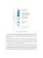
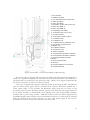
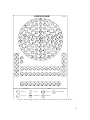
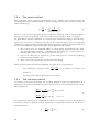
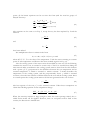
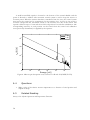
Student Reactor Exercises at VTT Version: 2008-01-08 Jarmo Ala-Heikkilä, TKK ([email protected]) Tom Serén, VTT ([email protected]) Calle Persson, KTH ([email protected]) (Partially adapted from Advanced Laboratory Exercises for TRIGA Research Reactor, TKK-F-C198 Rev.1, Espoo 2007 ©TKK,VTT) Copyright © 2007 by Helsinki University of Technology (TKK), VTT Technical Research Centre of Finland and the Royal Institute of Technology (KTH). All rights reserved. No part of this publication may be reproduced, stored in a retrieval system, or transmitted, in any form or by any means, electronic, mechanical, photocopying, recording, or otherwise, without prior written permission of the publisher. Foreword: How to use this document This document describes the various reactor exercises that will be performed in the KTH Reactor Physics course (SH2600) at the research reactor at the Technical Research Centre of Finland (VTT) located in Otaniemi, Espoo just outside Helsinki. First a description of the reactor is given. This part is supposed to make the reader familiar with the reactor at which the exercises will be performed. After the description of the reactor, a number of chapters describing the different exercises follow. These chapters are supposed to be studied carefully in advance before performing the exercises in order to be well prepared. Some of these chapters have some preparation tasks and questions in the end. Try to find answers to the preparation tasks before going to the reactor, since their solutions might be useful when the reactor exercises are carried out. The solutions to the preparation tasks do not have to be included in the final report but the answers to the questions in the question sections must be presented in some way, embedded in the text or separately. It is highly recommended to study the document Basic Data Handling in Nuclear and Reactor Applications [1] before performing the reactor exercises and definitely before performing any data analysis on the acquired data. By using the methods proposed in that document, the analysis of the experimental data will be much easier and you will save a lot of time. Finally, some words are given about how the report is expected to be written. Try to write the report as soon as possible after the exercises, since it is much easier to do it when things are still reachable in mind. Last but not least, be open-minded, try to be as active as possible during the exercises and have a nice time by the reactor and in Finland! 3 4 Table of Contents 1 2 3 4 5 6 7 8 9 10 Introduction................................................................................................................................ 7 Exercise: Reactor Start-up – Approach to Criticality .........................................................13 Exercise: Control Rod Calibration ........................................................................................17 Exercise: The Effect of Temperature on Reactivity ...........................................................21 Exercise: Determination of Delayed Neutron Precursor Groups....................................29 Exercise: Neutron Importance ..............................................................................................35 Exercise: Neutron Activation Techniques ...........................................................................37 Appendix A: Summary of Technical Properties of FiR 1..................................................47 Appendix B: Requirements for the Report ..........................................................................51 References .................................................................................................................................53 5 1 Introduction 1.1 The FiR 1 Reactor The FiR 1 (Finland Reactor 1) is a so-called swimming pool reactor of type TRIGA Mark II. The abbreviation TRIGA stands for Training, Research, Isotope production, General Atomics. The nominal thermal power is 250 kW (originally 100 kW until 1967). The reactor is operated by the Technical Research Centre of Finland (VTT) and is situated in the Otaniemi campus area in Espoo, Finland. The reactor was started in 1962 and the operator was originally Helsinki University of Technology (TKK) until 1972. The reactor core and graphite reflector are situated in a water tank, 6 m deep and 2 m in diameter. The water serves as heat transfer agent, as radiation shielding upwards and as moderator. However, most of the moderation takes place in the fuel itself. The TRIGA fuel consists of uranium metal enriched to 20%, alloyed with zirconium hydride. The hydrogen-zirconium ratio is about 1 and the uranium concentration is 8, 8.5 or 12% by weight. One fuel element contains between 36 and 54 g of 235U. The structure of a cylindrical fuel rod (or element) is shown in Figure 1. The cladding is either aluminum or stainless steel. The active part has a radius of about 21 cm and is 35.5 cm long and has a samarium plate at each end. The samarium plates serve as burnable absorbers, reducing the effect of reactor poisoning and burnup on the excess reactivity. There are graphite reflectors at each end. This type of fuel gives a fast negative temperature coefficient of reactivity, which makes the pulsing of the reactor possible, increases the safety of the reactor and makes it easy to operate. This is due to the special moderation properties of the zirconium-hydrogen system. It is possible to create (“shoot”) power pulses of 250 MW with duration of about 30 ms by making the reactor prompt supercritical. However, this has not been done for several years since large pulses put some strain on the fuel. The structure of the reactor core is shown in Figure 2 and Figure 3. The grid comprises some 80 fuel rods, 2 graphite rods, 4 control rods, a Sb-Be neutron source, a central thimble and a pneumatic transfer system (rabbit). The core grid contains about 35% water in addition to the fuel rods. The core loading is asymmetric with more 12%-fuel in the direction of the BNCT moderator. This increases the intensity of the BNCT beam by about 30% compared to a symmetric loading. Figure 1. A TRIGA fuel element [2]. The core is surrounded by a cylindrical graphite reflector containing a dry irradiation ring (“Lazy Susan”) with 40 positions. Radial radiation shielding is provided by 2.25 m of concrete, penetrated at core level by four beam tubes and a BNCT moderator (formerly a thermal column containing graphite). The beam tubes are plugged and have not been used for several years. The reactor is controlled with three boron carbide-filled control rods (attached to guide shafts) which move in their guide tubes, and with a boron graphite-filled pulse rod. The regulating and shim rods are moved with servo motors and the pulse rod with a pneumatic system. The pulse rod has only two positions: up and down. The pulse rod serves as a safety rod. The control rods are attached with electromagnets to the moving devices. A reactor scram cuts off the current from the holding magnets. In steady state operation the pulse rod is kept in the upper position and the power is controlled with the shim rods and the regulating rod. In pulse mode the reactor is first made critical with the shim and regulating rods and a sudden reactivity injection is brought about with the pulse rod. In normal mode the pulse rod is locked if any one of the other rods has been raised. The control rods are operated manually with push-buttons on the control desk. When operating at constant power the control can take place either manually or with an automatic control system which operates on the regulating rod (if needed also on Shim II). 8 1. Fuel element 2. Graphite element 3. & 4. Instrumented fuel elements 5. Upper grid plate 6. Lower grid plate 7. Pneumatic control rod (pulse rod) 8. Shim rod (SHIM I) 9. Shim rod (SHIM II) 10. Regulating rod (REG) 11. Activation tube (not in use) 12. Central channel 13. Pneumatic transfer system 14. Irradiation ring 15. Irradiation cup 16. Loading tube for irradiation ring 17. Circulation mechanism for irradiation ring 18. Graphite reflector 19. Aluminum cover 20. Fission chamber 21. Compensated ionization chamber 22. Compensated ionization chamber 23. Uncompensated ionization chamber 24. Piercing beam tube 25. Bellows 26. Support platform for reflector 27. Adjustment bolt Figure 2. The FiR 1 core and surrounding components [2]. The neutron flux is detected with one fission chamber and three ionization chambers, of which two are gamma-compensated. The pulse rate of the fission chamber is recorded with a rate meter and it is useful only at low power (0.1 mW - 100 W). If no signal is obtained from the fission counter the control rods cannot be raised. One of the compensated ionization chambers works in the range 30 mW - 300 kW and gives the linear power signal, which is recorded with a plotter. The linear channel has a scram signal switch. It also provides the difference signal (from the set value) to the automatic control system. The linear channel operates over several power ranges which can be set either manually or automatically (auto ranging). The other compensated ionization chamber with a power range 10 mW - 1000 kW is used to form the period signal and the logarithmic display signal, which is also recorded with the plotter. A scram signal is obtained from this channel if the positive period is too short. The period signal is also used to determine the correction rate of the automatic control system. 9 The uncompensated ionization chamber is connected to the safety channel and works properly only at higher powers (only one range 0 - 300 kW). A scram signal is also obtained from this channel. In pulse mode it is the only channel in use. In addition to the power (i.e., neutron flux) several other quantities are also measured and recorded: fuel temperature (with scram signal), water temperature, water level, water conductivity, water activity etc. There are several radiation monitors in the reactor hall and pump room which are connected to a LabView recording system. Cooling is provided with cooling towers and a heat exchanger between the primary and secondary circuit. Part of the primary water circulation always passes through a cleaning branch with a filter and ion exchange resins. The nuclear channels were manufactured by KFKI, Hungary, and the control electronics by Valmet Instrument Works, Finland (Elmatic analogue control system). The instrumentation was completely renewed in 1981. The BNCT beam has its own monitoring system with three fission chambers and an ionization chamber connected to a LabView system, which also communicates with the reactor instrumentation. There is a lockable scram button in the BNCT control room, but otherwise the reactor can only be operated from its own control desk. Since 1999 the FiR 1 reactor has been used mainly for Boron Neutron Capture Therapy (BNCT) treatment of cancer patients. For that purpose a moderator block containing FluentalTM material was designed and built to create an epithermal treatment beam. Also a well-shielded treatment room and a containment room above the reactor tank were built. Other uses of the reactor are production of industrial tracer isotopes and, to a lesser extent, activation analysis and education and training of students, mainly from TKK. 10 LOADING SCHEME E24 2535 F4 2523 E2 2545 E23 F27 2533 E3 2495 2504 E22 2530 D18 D17 2519 E21 2517 F25 2497 E4 4166 C12 2526 F24 D15 4205 B6 4152 C10 2509 E19 2524 D14 4188 2539 INSTR 6575 B5 E18 SHIM I 6536 CENTRAL TUBE 6554 F8 D5 B2 6545 C4 A1 6550 E7 6538 B3 6558 6544 D6 F9 6539 C5 6548 E8 C8 6542 C7 2499 D12 INSTR 2345 E16 2575 2527 4154 D9 PS 2522 F12 2532 E11 2525 E14 2502 6556 F11 2492 E10 D10 E15 2538 E12 2546 2513 F13 E13 F19 T1 2349 1894 INSTR 4312 F10 6546 E9 D8 2547 D11 2574 F20 6552 D7 6540 C6 2493 2505 E17 F18 2516 F17 W1 2520 F7 6549 E6 C3 6557 2555 D13 T12 6551 6535 6543 B4 C9 2536 F22 2529 6553 6537 B1 4186 C11 2552 2521 F21 6541 C2 F6 6547 E5 D4 E20 F23 C1 D16 REG 6555 4173 D3 SHIM II 2515 2496 F5 2498 D2 D1 2494 F26 NEUTRON SOURCE F2 2512 E1 2549 PNEUMATIC TRANS. 2506 F1 F3 2528 F28 2514 2354 2544 F30 2542 F29 20.09.2005 1898 F16 GRAF F14 2543 F15 T11 T2 INSTR 2344 W2 2550 T3 T10 T9 2531 T4 GRAF M20 GRAF M19 M18 M17 M16 M15 1877 M14 M13 M12 M11 2507 T8 T5 L20 T7 L40 2070 L19 L18 2518 L39 L38 L17 L16 L14 L13 L12 L11 T6 2508 L37 L36 FUEL ELEMENTS L35 L34 L33 L32 L31 OTHERS SS-CLAD,12%U SS-CLAD,8,5%U L15 INSTR STR AL-CLAD,8%U CONTROL ROD INSTRUMENTED OTHER DEVICE GRAF GRAPHITE ELEMENT Figure 3. The loading scheme of the FiR 1 reactor (situation as of Sep 20, 2005). 11 2 Exercise: Reactor Start-up – Approach to Criticality 2.1 Objective When starting a reactor for the first time, for instance after refueling, the critical level of the control rods is not known. Therefore, the control rod withdrawal must be done carefully in order to avoid super-criticality and an unexpected power excursion. In this exercise, the critical level of the control rods will be determined by monitoring the neutron flux in the core while withdrawing the control rods. This is a common safety procedure always performed at first start-up of reactors. 2.2 Background: Neutron Multiplication Consider the introduction of S source neutrons into a subcritical reactor with multiplication factor k. There will be S·k neutrons after the first fission generation, S·k2 neutrons after the second generation, and so on, so that the total number of neutrons per source neutrons after many generations, approaches a geometrical series: M= (1 + k + k 2 + …) S S = 1 1− k (1) Here, M is called the source multiplication, describing the ratio of the fission source to the external source and gives consequently the total number of neutrons appearing in the fissionable material per source neutron. Please note that since the expression above is valid for a subcritical system, k is smaller than one. It is seen that both the reciprocal source multiplication factor, 1/M, and 1-k decrease when approaching criticality: 1 = 1− k . M (2) This relationship is often employed in bringing a reactor system to criticality, by extrapolating to the critical condition. If, for example, the operator starts withdrawing control rods, the multiplication constant, and thus the source multiplication factor M, increases with increasing rod withdrawal. When the reactor reaches critical condition, the source multiplication factor becomes infinite. This ‘approach to criticality’ is monitored by placing a neutron source in the reactor and measuring the neutron flux for various rod positions. The neutron count rate is proportional to M. A plot of the inverse counting rate or 1/M as a function of rod position becomes equal to zero at the critical condition. If we extrapolate a curve to the zero value then we can pre-determine the control rod position at which the critical condition will be reached. In the discussion, it is assumed that the reactor is reasonably close to critical and that the neutron population is in equilibrium. If the reactor is far below critical then Eq. (2) is not valid. Eq. (2) only applies to the multiplication of neutrons in the eigenstate. Eigenstate in this sense, refers to neutrons such that their energy spectrum and spatial distribution are characteristic of the reactor, i.e. asymptotic spectrum, so called fundamental mode distribution, and with an effective multiplication factor keff. Source neutrons, in general, do not have these properties and multiply differently compared to eigenstate neutrons. In that case, we cannot formulate a simple geometric series, based on a single k-value. In close-to-critical conditions, this effect has negligible influence since source neutrons are small in number in comparison to the total neutron population. The neutron flux is characterized by the eigenstate at criticality. Although the measurement of source multiplication is a static technique, there are timedependent effects that can be important in the interpretation of results. The multiplication following a reactivity change (e.g. change in control rod position) in a subcritical system is observed only after all delayed neutrons have attained equilibrium concentration. During a sequence of stepwise addition of reactivity, as in following “1/M” approach to criticality, the total asymptotic multiplication will clearly be observed at each step if one waits sufficiently long after each reactivity addition. Nevertheless, if reactivity is added too rapidly – either stepwise or continuously – the observed multiplication will lag the asymptotic multiplication thus giving an underestimate of the instantaneous multiplication of the system. The physical reason for this transient effect is clear. The equilibrium condition is identified by a selfsustained constant power level only when all delayed neutron precursors are in equilibrium, meaning that the formation rate of delayed neutron precursors equals the decay rate. Under very weak source conditions, the neutron level during the early stages of startup is so low that statistical fluctuations tend to dominate and the kinetic equations are not applicable. At later stages, the power level becomes sufficiently high and statistical fluctuations are no longer important. In general, distorting effects become relatively small near criticality and extrapolated critical points become progressively more reliable as the critical condition is approached. 2.3 Experimental Procedure The basic requirements for this measurement are a neutron source, either inherent in the fuel or added to it, and a neutron detector (the FiR 1 reactor has a permanently installed neutron source). If these requirements are satisfied, the detector count rate under equilibrium conditions is proportional to the neutron multiplication, and its reciprocal approaches zero as the reactor approaches the critical state. The detector count rate or signal strength (in current mode), N, is given by 14 N = (1 + k + k 2 + …) ε S = εS 1− k (3) where ε is the efficiency of the detector. The reactor power can be assumed to be proportional to N (the readings of the reactor instrumentation are in power units). As for M-1, N-1 will approach zero when k approaches 1. The criticality approach curve (e.g. the reciprocal count rate, N-1, as a function of reactivity insertion) is then used to predict the critical control rod height. It is desirable to monitor the approach, and analyze the data continuously, to ensure that the approach is orderly and to determine whether the reactor is far from or close to the critical state. Follow these steps to reach criticality: 1. At the start of the exercise the control rods are fully inserted into the core. Read the water temperature in the pool. 2. With the pulse rod in the UP position, the SHIM I and SHIM II in suitable positions (will depend on the operating history) and the REG rod in the DN position (0 %), note the LIN power reading after the situation has stabilized. 3. Raise the REG rod in steps (e.g. 20 %, 30 %, 35 % and 40 %) and note the new detector count rate after stabilization. Sufficient time must be allowed at each step for the power to stabilize. 4. Read the REG rod insertion to each step from the calibration curve. Plot the reciprocal count rate (power), N-1, as a function of contgrol rod position, and make a linear extrapolation to zero to find the critical control rod height (Figure 4). 5. Ask the operator to move the REG rod to a position below the expected critical height. Observe the behavior of the reactor. 15 N-1 ■ ■ Inverse count rate hi hi+1 control rod height hc,i h Figure 4. Description of the linear extrapolation used in the subcritical approach (i=0,1,2,3…). 2.4 Preparation Task 1. Give an expression for the expected critical control rod position hc,i for a given hi and hi+1 (Figure 4). 2.5 Questions 1. Why is the subcritical approach performed using an external neutron source? There are neutrons released in the fuel through for instance spontaneous fissions and (α,xn)-reactions. 2. When plotting the data from the experiment, you will find that the linear dependence is not valid for all control rod height. Try to explain why the linear dependence is valid only close to criticality. 3. Why does it take longer time to reach the equilibrium condition as criticality is approached? 2.6 Related Reading On the Reactor Physics CD: The Chain Reaction and Multiplication of Neutrons, pp. 1-9. Reactor Dynamics, pp. 28-30. 16 3 Exercise: Control Rod Calibration 3.1 Objective Control rods are used in reactors to change the power, perform shut downs and to make sure that the core at any moment can be made sufficiently subcritical. The rods are grouped according to their function and located at different places in the core where their function is maximized. In this exercise, the regulation rod will be calibrated, i.e. the reactivity that corresponds to a certain control rod movement will be found. 3.2 Control Rods and Calibration Methods A reactor is usually equipped with three types of control rods: 1. The safety rod is lifted entirely during normal use. It is used for quick shut-down of the reactor. Usually it is possible to control the reactor only when the safety rod is completely lifted out of the core. Power reactors cannot be made critical with the safety rod inserted. However, in some research reactors with a fast negative temperature reactivity feedback this has been made possible. In that case the fast withdrawal of the safety rod from a critical reactor will lead to a very fast rise in power, which is almost immediately stopped by the feedback. This is called a neutron pulse, and the safety rod serves as a pulse rod. This is the case in The FiR 1 TRIGA. 2. A shim rod (coarse rod) is mainly used to compensate slow changes in reactivity caused, e.g., by fuel burnup and reactor poisoning. 3. A regulating rod is used for fine-tuning the reactor power level and to compensate occasional reactivity changes. The automatic control system of the reactor keeps the power constant by moving the regulating rod. In FiR 1 the SHIM II rod can also participate in the automatic control if needed (e.g. during long runs with significant poisoning). A control rod can be calibrated based on two methods: the period method and the rod drop method. These methods are described below. 17 3.2.1 The period method This technique utilizes period measurements in the slightly super-critical region. By measuring the reactor period followed a reactivity change, the reactivity is found by using the inhour equation [3]: ρ= 6 ⎛ βi 1⎛ Λ + ⎜⎜ ⎜ ∑ T⎝ i =1 ⎝ 1/ T + λi ⎞⎞ ⎟ ⎟⎟ , ⎠⎠ (4) where Λ is the neutron reproduction time (frequently called the mean neutron generation time) and T is the reactor period. Values for βi and λi can be found in Table 1 on page 32. An approximate reactivity calibration of a control rod is obtained according to the following: Operate the reactor at a constant power. The power should be kept low to avoid thermal feedbacks, but high enough to ensure stable reactor operation. Position the control rods that are not to be calibrated at equal axial height and the REG rod fully inserted. 1) The control rod to be calibrated (REG) is raised quickly approximately 20% units. The corresponding reactivity is obtained by measuring the reactor period (or doubling time) and by using the inhour equation, Eq. (4). 2) One of the shim rods is adjusted to get the same power as from the beginning, without moving the REG rod. 3) Tasks 1 and 2 are repeated for the full control rod length. When the full control rod has been calibrated, two plots are to be performed: ∂ρ Δρ ≈ , as a function of control rod − The differential reactivity worth, ∂z Δz position, z. − The integrated control rod reactivity worth, ρtot(z). 3.2.2 The rod drop method In contrast to the previous method, the rod drop method is based on measurements in a subcritical core. The time dependent neutron flux in a reactor can be described by the pointkinetic equations: 6 ⎧ dn(t ) ρ − β eff = + λi Ci (t ) + S (t ) n ( t ) ∑ ⎪⎪ Λ dt i =1 ⎨ ⎪ dci (t ) = βi n(t ) − λ C (t ), i = 1, 2...6 i i ⎪⎩ dt Λ (5) In a steady state reactor (ρ=0) at equilibrium at flux level n0 without sources, the production of neutrons from the delayed neutron precursors is completely balanced by the decay of prompt neutrons: 0=− 18 β eff Λ 6 n0 + ∑ λi Ci ,0 . i =1 (6) Assume that a control rod is quickly inserted bringing the core to a subcritical state. If this reactivity withdrawal is fast enough, the delayed neutron precursor density may be assumed to be the same immediately after the rod drop as before. If neglecting details about the prompt neutrons during the prompt jump, the time derivative can be set to zero. However, the neutron flux level, n1, will be drastically lower since the core is subcritical. The situation is described by the point-kinetic equations as: 0= ρ1 − β eff Λ 6 n1 + ∑ λi Ci ,0 . (7) i =1 By rearranging Eqs. (6) and (7) the following relation is achieved: n ρ1 =1− 0 . n1 β eff (8) Eq. (8) can consequently be used to find the reactivity of the quickly inserted control rod by measuring the neutron flux before and immediately after the rod drop. In this exercise it is done in the following manner: 1) The control rod to be calibrated (REG) is completely withdrawn (100%). 2) Note the detector reading. 3) Let the REG rod drop to 0% and note the detector reading again. 4) Raise the REG rod to 75%, 50% and 25% and perform tasks 2 and 3 repeatedly. 5) Plot the total reactivity removal as a function of the original control rod position. 3.3 Determination of the shutdown margin The shutdown margin is defined by the margin to criticality under the condition where the most reactive control rod remains in the top position. Besides the reactivity worth of the control rods, the shutdown margin, M, depends on poisoning and on water temperature, according to Eq. (9). actual ∂ρi ∂ρ ∂ρ M =∑ ∫ dz − ∫ dT − df ∫ ∂T ∂f i in core ∂z cold non − poisoned poisoned (9) In this equation, i is the index for all control rods except the most reactive, T is the water temperature and f is the poisoning. The differential reactivity worth, ∂ρ i , ∂z is obtained from the control rod calibration. Assume that all control rods have the same reactivity worth. It can be assumed that the water temperature does not fall below 20 °C and that the reactor is not poisoned. 19 3.4 Determination of the Excess Reactivity All reactors have a certain amount of built-in excess reactivity, to compensate for burnup and poisoning. We may estimate this excess reactivity, R, for the TRIGA reactor using Eq. (10): R=∑ i ∂ρ i dz . ∂ z criticality top ∫ (10) In this equation, i is the index of all control rods. The integral is calculated using measured data on the differential control rod reactivity worth and the calculated value is an indication of the burnup potential. Assume that all control rods has the same reactivity worth. What is the corresponding value of keff? 3.5 Preparation tasks 1. What is the meaning of the reactor period and the doubling time? What is the reactor period of a critical reactor? 2. Write a function, preferably in MATLAB, that takes the reactor period as an input parameter and delivers the reactivity (based on Eq. (4)). 3.6 Questions 1. Why must the control rods be calibrated from time to time? 2. What method was the most accurate one? The period method or the rod drop method? 3.7 Related Reading On the Reactor Physics CD: Reactor Kinetics Stacey: 5.2 – 5.4 (Point kinetics and the inhour equation) 20 4 Exercise: The Effect of Temperature on Reactivity 4.1 General Considerations The power of a nuclear reactor stays constant when the multiplication factor keff = 1. At constant power the cooling system of the reactor removes all the heat that is generated. If the multiplication factor is increased by Δkeff = keff−1 > 0, the power of the reactor starts to grow at a rate determined by the magnitude of Δkeff. The cooling system cannot, at least immediately, absorb all the thermal energy released in fission, but part of it will raise the temperature of the reactor core. In the absence of any limiting factors the temperature would rise indefinitely, and finally the core would melt. In cases like this the temperature dependence of the reactivity ρ = Δkeff /keff and the feedback caused by it usually constitute a limiting factor. The dependence of the reactivity on temperature is described by the temperature coefficient of the reactivity. For this we have to assume that the whole reactor core can be characterized by one single temperature T. The temperature coefficient α is defined as a derivative: α= dρ . dT (11) Usually it is assumed that when ρ is expanded into a series of (T−T0), the series can be truncated after the first-degree term, i.e., we have a linear relationship. Here T0 is some suitable reference temperature. α is usually expressed in units °C-1, less frequently $/°C. If the temperature coefficient α is negative, i.e., the reactivity decreases as the temperature increases, the reactor will behave stably. When the multiplication factor for some reason or other undergoes a positive change the neutron flux and thus also the power starts to rise. Since all the heat generated is not removed from the reactor the core temperature will rise. This reduces the reactivity and slows down the increase in power. Finally the temperature reaches a level where it is sufficient to compensate the whole original 21 reactivity insertion. The power will stop increasing and with still rising temperature will start decreasing. Finally, the system will stabilize at a new power level between the original level and the power peak. Such a behavior is, of course, highly desirable for safety reasons. It is easy to accomplish reactor designs which lead to increased reactivity with rising temperature and, as a consequence, are inherently unstable. Chernobyl provides a horrendous example. However, merely a negative temperature coefficient is not a sufficient guarantee for safe operation. Often there is a delay in the feedback between power increase and reduced reactivity. This delay is usually caused by the time needed for heat transfer or, e.g., for expelling the excess water volume created by thermal expansion from the core. If a reactor achieves strong prompt criticality the power increase will be extremely fast. The heat transfer from the fuel elements to the coolant and moderator is then far too slow to have an influence on phenomena whose time behavior is determined by the neutron life-time in the core. The phenomena associated with the expulsion of matter from the core also require a time which is of the same order as the reactor dimensions divided by the speed of sound. For a reactor to be safe even in a prompt critical state one must, therefore, require that the temperature coefficient of reactivity is not only negative but also fast. By fast we here mean a time which is short compared to the neutron life-time. 4.2 The Fast Temperature Coefficient The fast or prompt temperature coefficient stems from phenomena associated with the changes in the reactor physical properties caused by heating of the fuel. The fast negative temperature coefficient of the FiR 1 TRIGA Mark II reactor is achieved with the semihomogeneous structure and the zirconium hydride in the fuel. Nearly all hitherto constructed reactors have a fast negative temperature coefficient of reactivity, and licensing authorities do not generally allow the construction of reactors without this property. In the TRIGA Mark II reactor only the fast temperature coefficient is negative. Thus, if the core and cooling water are heated homogeneously and simultaneously, one can observe an increase rather than a decrease in reactivity. The fact that during normal operating conditions the reactivity decreases with increasing power is thus exclusively a consequence of the rise in temperature difference between the fuel and coolant caused by the increased heat flow. This type of behavior is very desirable from the reactor technical point of view, since no excess reactivity is needed to compensate reactivity loss when going from a cold reactor core to the operational temperature. Three effects contributing to the fast negative temperature coefficient in the TRIGA have been identified: 1. Doppler broadening 2. Increased neutron leakage 3. The Dyson effect 4.2.1 Doppler broadening With rising fuel temperature the thermal motion of the nuclei increases. As a consequence a neutron moving with constant speed in the fuel will encounter fuel nuclei whose movement 22 in the direction of the neutrons movement will follow a Maxwellian distribution. This leads to a broadening of the resonance peaks in the absorption cross sections, so-called Doppler broadening. The probability of parasitic absorption of the neutron during slowing-down increases. This in turn decreases the resonance escape probability, the multiplication factor and the reactivity. This phenomenon is prompt. 4.2.2 Increased neutron leakage The increase in neutron leakage is caused by the dependence of the thermal cross sections on the fuel temperature. With rising temperature the diffusion length will increase (in fact the TRIGA is a reflected reactor, which means that this effect can be interpreted as a decrease in the fraction of neutrons returning to the core, but qualitatively the following reasoning is valid). The temperature dependence of the cross sections can be treated quantitatively if the neutron spectrum in the reactor can be determined. The shape of the spectrum is determined by the slowing-down properties of the water and the zirconium hydride. Both are well-known, although complicated to handle theoretically. The slowing-down process in the zirconium hydride is especially interesting. It can be shown that the so-called Einstein model is valid for this material. In this model the hydrogen atoms are assumed to be quantized harmonic oscillators in thermal equilibrium with the fuel. This proposition is natural since the hydrogen atoms are situated as interstitials in a surface-centered zirconium grid at the centre points of a tetrahedron formed by the zirconium atoms. Thus they are capable of oscillating independent of each other with the harmonic force as a good first approximation for the real restoring force. By using the Einstein model for the zirconium hydride and a Maxwellian velocity distribution for the neutrons slowed down by the water the average thermal neutron cross sections can be calculated as a function of temperature. In this treatment it must be assumed that the temperature of the coolant water does not change. It is obvious that this effect is also fast since the slowing-down time is short compared to the diffusion time. 4.2.3 The Dyson effect The Dyson effect is based on the fact that the spectrum of neutrons coming from a hot fuel is harder than the spectrum at lower powers. When reaching the surrounding water, still at its original temperature, the neutrons will immediately slow down to a Maxwellian distribution corresponding to the water temperature. Thus the number of absorptions in the fuel will decrease because the cross sections become smaller as the fuel temperature increases, but the number of absorptions in the water will remain the same. This leads to a fast degradation of the thermal utilization factor and a reduction in reactivity 4.2.4 The basic equations In the following we shall try to analyze in more depth the behavior of a reactor that has been running at constant power for a long time after which its multiplication factor is quickly increased, e.g., by raising a control rod. The fast temperature coefficient of reactivity is assumed to be negative. For this purpose the kinetic behavior of the reactor must be described with some model. In practice this can usually be accomplished with the aid of the so-called point kinetic equations, originally derived for an infinite reactor [4]. Moving from neutron density to 23 power (P) the kinetic equations can be cast into the form (with the usual six groups of delayed neutrons): 6 dP keff (1 − β eff ) − 1 = P + ∑ λi Ci (t ) dt l i =1 . β i keff dCi = −λi Ci + P, (i = 1, 2...6) dt l (12) The notations are the same as in Eqs. 5, except that n(t) has been replaced by P and the relations ρ= keff − 1 keff (13) and keff = l Λ (14) have been utilized. The multiplication factor is written in the form: keff = 1 + Δkeff + α (T − T0 ) ≅ 1 + ρ + αΔT (15) where ΔT=T−T0. T0 is the value of the temperature T with the reactor running at constant power P0. The temperature coefficient α has been assumed negative in Eq. (15). Also the cooling system of the reactor must be modeled in some way. In the following treatment the reactor core is assumed to consist only of fuel. It is assumed that during the time interval under consideration the cooling system removes heat from the fuel elements with a power γ(T−Te) proportional to the difference between the core temperature and an external temperature Te which is assumed to remain constant. Te mainly describes the temperature of the cooling system, and the proportionality factor γ, which is assumed constant, is then the heat transfer coefficient between the core and the cooling system. Since at constant power the cooling system removes all the heat generated in the core we have: γ= P0 T0 − Te (16) The heat capacity of the core, C, is also assumed constant. Under these assumptions we obtain the following equation for the temperature change: d ΔT P − γ (T − Te ) P − P0 − γΔT = = dt C C (17) When the reactivity injection is large enough to make the reactor prompt critical, the socalled Fuchs model can be applied. However, since no real pulses will be fired in this exercise, the discussion is omitted here. 24 4.3 The Influence of the Temperature Coefficient on the Prompt Jump When the multiplication factor of the reactor is increased moderately, so that it does not become prompt critical, the power increase remains manageable even without the aid of the temperature coefficient. The power initially grows quickly (the so-called prompt jump), but very soon it starts to exponentially approach its asymptotic value [4]: Pas = β β −ρ P0 . (18) Because of the delayed neutrons the power will, however, not settle at this value, but continues to grow slowly. The influence of the temperature coefficient becomes visible if P0 is large or β−ρ is very small. The power then after a certain time reaches a maximum, after which it will fall somewhat and finally stabilize at a level determined by P∞ = P0 + γ P. −α (19) A few typical slow pulses measured at FiR 1 are sketched in Figure 5. Figure 5. Slow pulses at FiR 1. 25 4.4 Determining the Fast Temperature Coefficient of Reactivity In this exercise the fast temperature coefficient of reactivity, i.e., the temperature coefficient of the fuel, is measured. The procedure is as follows: The reactor power is stabilized at about 40 kW with the control rod Shim I at a fixed position (usually 50%). The Shim II and Reg rods are used to reach this power level. The automatic control system can be used to achieve this quickly. The automatic control is switched off when a stable power level has been reached. By quickly raising the Shim I rod by about 5% a reactivity of 5–20 c is injected into the reactor. The change in power as a function of time is recorded on the linear channel plotter. The speed of the plotter is set at 10 cm/min (in this case the speed is significant). This is repeated a few times. For each pulse the change in Shim I position should be recorded, because it will probably differ somewhat from pulse to pulse. The results can be used to determine the fast temperature coefficient of reactivity according to the following calculational methods. 4.4.1 Determining the temperature coefficient We assume that the reactivity ρ is a function of the time t and the core temperature T: ρ = ρ (t , T ) . (20) ⎛ ∂ρ ⎞ ⎛ ∂ρ ⎞ ⎛ ∂ρ ⎞ d ρ = ⎜ ⎟ dt + ⎜ ⎟ dT = ⎜ ⎟ dt + αΔT . ⎝ ∂t ⎠T ⎝ ∂T ⎠t ⎝ ∂t ⎠T (21) By differentiating we obtain: Integrating Eq. (21) from 0 to time t and assuming that α remains constant during this time interval, and denoting T(t)−T(0) = ΔT(t), we obtain: ⎛ ∂ρ ⎞ ⎟ dt + αΔT (t ) . ∂t ⎠T 0⎝ t ρ (t ) − ρ (0) = ∫ ⎜ (22) Let us now further assume that ρ(t, T(t)) can be written as the sum of a time-dependent part and a temperature-dependent part: ρ (t , T ) = ρt + ρT . (23) From Eqs. (22) and (23) we then obtain: ρ (t ) − ρ (0) = δρt + αΔT (t ) . (24) where δρt is the increase in the time-dependent reactivity (injected with the control rod) during time 0 → t. How this change is brought about is not important. When measuring the temperature coefficient we have ρ(0) = ρt(0) = 0. The time-dependent reactivity ρt receives its whole constant value δρt almost instantaneously at t = 0. When we measure ΔT(t0), the change in T going from t = 0 to t0, we obtain α from the equation: 26 α= ρ (t0 ) − δρt ΔT (t0 ) . (25) It is advantageous to choose t0 as the maximum point of the power curve. 4.4.2 Determining ρ(t0) a) A coarse estimate. A very coarse estimate for ρ(t0) is obtained by assuming that all neutrons emitted in fission are prompt, i.e., β = 0. We thus assume that the power increases so slowly that the neutron mean lifetime can be considered a very small quantity. According to Eq. (11) we then obtain: dP ρ = P, dt l (26) ρ (t0 ) = 0 . (27) and at the peak of the pulse: Naturally, the slower the pulse, the better this approximation will be, but on the other hand the heat transfer models become less and less useful as the duration of the phenomenon increases. b) A more accurate estimate. The delayed neutrons can also be accounted for exactly [5]. From Eq. (12) we can solve Ci(t): ⎡ ⎤ β t Ci (t ) = e − λi t ⎢Ci (0) + ∫ eλi t keff P(t )dt ⎥ . l 0 ⎣ ⎦ (28) When this is inserted into Eq. 12, and taking into account that 6 ∑ λ C (0) = i =1 i i β l P0 , (29) we have: 6 β dP 1− β β P(t ) − ( P(t ) − P0 ) + ∑ i e − λi t ∫ eλi t ( keff P(t ) − P0 ) λi dt . =ρ dt l l i =1 l 0 t (30) At the maximum, this expression equals zero. Inside the integral we can set keff = 1 to obtain: ρ (t0 ) = 1 (1 − β ) P eff max t0 6 ⎛ ⎞ −λ t λt ⎜⎜ β eff ( Pmax − P0 ) − ∑ β i e i 0 ∫ e i ( P(t ) − P0 ) λi dt ⎟⎟ . i =1 0 ⎝ ⎠ (31) In evaluating the integral in the above formula one must resort to approximate methods. It is then worth noting that the major part of the integrals value comes from the region near the peak of the pulse. In this exercise the more exact method b) should be used to evaluate the results. 27 4.4.3 Determining ΔT(t0) One could try to measure the rise in temperature ΔT(t0) directly if one could unambiguously establish what temperature the quantity T most closely describes. However ΔT(t0) can also be calculated from the heat transfer model by integrating Eq. (17): ΔT (t0 ) = 1 γ e − μ t0 t0 μ ∫ e ( P(t ) − P ) μ dt , t0 0 (32) 0 where we have denoted μ = γ/C. However, the value of the coefficient γ is usually not known. In principle it could be obtained as the ratio between P0 and (T0−Te), but because of the hypothetical nature of these temperatures their magnitude is difficult to determine. Usually one must assume the cooling system to be slow (as is done in the Fuchs model), in which case we can set γ = 0. Then ΔT(t0) can be solved from the equation: t ΔT (t0 ) = 1 0 ( P(t ) − P0 ) dt , C ∫0 (33) The significance of leaving out γ can be evaluated by assuming that Te represents the average temperature of the cooling water in the tank and T represents the spatial average of the fuel temperature. 4.5 Questions 1. Shortly describe the measurements. 2. From the measured power pulses, calculate the fast temperature coefficient of reactivity using the methods presented above (ρ(T0) by method b). 4.6 Related Reading On the Reactor Physics CD: Reactor Dynamics, pp. 1-14. Stacey: 5.7 Reactivity Feedback (overview) 28 5 Exercise: Determination of Delayed Neutron Precursor Groups 5.1 Objective Delayed neutrons, i.e. neutrons released by the decay of fission products a considerable time after the fission event, are essential for the control of the reactor. Although the fraction of delayed neutrons is very low, its influence on reactor kinetics and thereby reactor control is of vital importance. In this exercise, the time behavior of delayed neutrons will become clear and some groups of delayed neutron precursors will be identified according to their different decay rates. 5.2 Delayed Neutrons In the fission process, in general, two or three neutrons are released immediately. These neutrons are referred to as prompt neutrons. The fission products, on the other hand, are in general unstable and may decay with a direct or subsequent emission of a neutron. For instance, consider the fission product “X”. This nucleus will, most probably, be a neutron rich nucleus that will undergo one or several β-decays to reduce its neutron excess. The “X”nucleus or one of the nuclei in its decay chain may then release a neutron, following the decay scheme below: A Z − β A X N ⎯⎯ → Z+1 YN-1 ⎯⎯ → A-1 Z+1TN-2 + n . The “X”-nucleus is called delayed neutron precursor and the “Y”-nucleus is the delayed neutron emitter (sometimes the precursor and the emitter is the same nucleus). The time from the fission event to the emitting of the delayed neutron depends on the half-life of the delayed neutron precursor and possible intermediate steps. However, important is the extremely large difference in time compared to the prompt neutrons, which are released within less than 10-15 s after the fission event. The delayed neutrons are in general released several seconds or minutes later. An example is the reaction below: 87 − β ,t1/ 2 = 55.60 s Br ⎯⎯⎯⎯⎯ → 87 Kr* ⎯⎯ → 86 Kr + n(0.3 MeV) . 29 In Figure 6 the relative abundance of fission products is depicted. From the figure it is clear that from thermal fission in 235U, fission products with mass number in the regions around 90 and 130 are the most abundant. Consequently, in these regions the most important delayed neutron precursors are found. Examples of important delayed neutron precursors are isotopes of the elements Br, I, Rb and Kr. In total, there are approximately 40 delayed neutron precursors among the fission products [6]. The total number of neutrons released after a fission event, ν, is the sum of the prompt fission neutrons yield, νp, and the delayed neutron yield, νd. ν = ν p +ν d (34) The delayed neutron fraction is defined as β= νd ν p +ν d = νd ν (35) and its value is dependent both on the fissioned nucleus and the incoming neutron energy. In general it can be stated that the value of the delayed neutron fraction increases with the mass number A for a certain element (constant Z) and decreases for increasing Z (heavier elements). For thermal fission in 235U, the delayed neutron fraction is 0.0065 or 650 pcm (parts pro cent milles, 10-5). The energy of the delayed neutrons depends on the reaction from which the neutron originates. In general this energy is in the order of some hundreds keV and, consequently, less than the average energy of the fission Watt spectrum (1-2 MeV). Therefore, in a thermal system, the delayed neutrons are more efficient in causing further fissions than the fission neutrons since the delayed neutrons have smaller probability for absorption in 238U during slowing-down. Taking this efficiency into account, the effective delayed neutron fraction, βeff, has been introduced. In general, for a thermal reactor βeff > β, and in a fast reactor βeff < β. Figure 6. Fission product yield from fission of various nuclides [7]. 30 5.2.1 The delayed neutron groups To simplify the analysis of the time dependence of the delayed neutrons, they have been divided into six groups according to the half-life of all known delayed neutron precursors. Each group is characterized by an effective half-life, mean energy and delayed neutron yield. Values for thermal fission in 235U are given in Table 1. Assume a uranium fuelled reactor that has been operating for an infinite time in a critical state. In such a system, an equilibrium level of delayed neutrons has been accumulated. According to point-kinetics, the neutron flux after a sudden reactivity insertion is given by λρ ρ − β eff 6 ⎛ ρ t β i − ρ −i βi t ⎞ Λ n(t ) = n0 ⎜ e e −∑ ⎟. ⎜ ρ − β eff ⎟ i =1 ρ − β i ⎝ ⎠ (36) The time characteristics of the first term is governed by the neutron reproduction time of the prompt neutrons, Λ, which means that this term acts much faster than the other ones governed by the delayed neutrons. After a reactor shut-down, scram, one may assume that ρ β eff and Eq. (36) may after the decay of the prompt neutrons be approximated as ⎛ 6 βi ⎞ n(t ) = n0 ⎜ −∑ e − λi t ⎟ . ⎝ i =1 ρ − β i ⎠ (37) This equation can be approximated as a series of exponentials: 6 n(t ) = ∑ Ai e − λi t . (38) i =1 Consequently, by fitting of exponentials to neutron flux data after reactor scram, the decay constants of the delayed neutron precursors can be found. A typical detector signal after reactor scram is depicted in Figure 7. At t=90 the reactor is scrammed and the neutron flux decays rapidly due to the prompt neutron decay. Then the delayed contribution become visible (in the logarithmic scale). Linear scale Logarithmic scale 3 180 10 160 2 10 120 Count rate [s-1] Count rate [s-1] 140 100 80 60 40 1 10 0 10 -1 10 20 0 -2 0 50 100 150 200 Time [s] 250 300 350 10 0 50 100 150 200 250 300 350 Time [s] Figure 7. Typical detector count rate after reactor scram (fast shut-down). 31 Table 1. Delayed neutron data for thermal fission in 235U [6][ 8]. Half-life1, [s] [s ] Mean energy [keV] 1 54.6±0.9 0.0127±0.0002 250±20 0.060±0.005 21.5 2 21.9±0.6 0.0317±0.0008 460±10 0.364±0.0013 142.4 3 6.0±0.2 0.115±0.003 405±20 0.349±0.024 127.4 4 2.23±0.06 0.311±0.008 450±20 0.628±0.015 256.8 5 0.50±0.03 1.40±0.081 - 0.179±0.014 74.8 6 0.18±0.02 3.87±0.37 - 0.070±0.005 27.3 Group t1/2 Decay constant, λi -1 Yield, νi Fraction, βi [n/fissions×100] [pcm] 1The values are calculated from the decay constants, which are the true experimental values, through the relation t 1/ 2 = ln(2)/ λi . 5.3 Experimental Procedure Firstly, the reactor is operating at high constant power level for a couple of minutes in order to achieve an equilibrium level of delayed neutron precursors in the system. If the power level is high, the count rate after shut-down will be higher and better statistics will be achieved. The neutron flux is measured by the neutron detector and the detector signal is stored digitally on a hard-drive. After a sudden shut-down, scram, of the reactor, the signal is still sampled for a couple of minutes in order to get data from the most long-lived delayed neutron groups. After some time, the count rate will be very low and the data acquisition can be stopped. The flux level as a function of time is recorded with a LabView system with recording intervals of about one second. This is sufficiently short to avoid histogram distortions for the more long-lived groups. 5.4 Data Processing By analyzing the experimental data using a non-linear function fitting tool, such as MINUIT from CERN [9], all twelve unknown parameters of Eq. (38) can in principle be found. Some commercial plotting packages, such as SigmaPlot [10] also have this capability. However, the use of such advanced analyzing tools is beyond the scope of this course. Another often used alternative method is to use linear function fitting. When doing so, the function fit of a single exponential must be performed in a region where all other exponentials can be neglected and the exponential of interest is isolated, preferably the most long-lived exponential. Try to find as many exponentials as possible by using the following iterative method: 1. Plot the detector signal after reactor scram and try to find the most long lived contributor to the signal by fitting an exponential function to the very last part of the data. Calculate χ2/ν and vary the start and stop values of your fitting to find the optimal interval. When the optimal interval has been found, calculate the statistical error of your result. 2. Remove the contribution from the most long-lived exponential by subtracting its contribution from the complete set of experimental data. When doing so, the statistical error of the data points is changed. Calculate this new error of each data point using the Propagation of Error Formula. 3. Perform step 1 and 2 until no more exponentials can be found. Values of the decay rates λi or half-lives and their corresponding standard deviations are to be calculated. 5.5 Preparation Task 1. Approximately how long time shall data be acquisitioned after reactor scram? 5.6 Questions 1. Describe why delayed neutrons are important for reactor operation and safety. 2. Try to explain how the effective delayed neutron fraction evolves with the burnup in a power producing nuclear reactor. 5.7 Related Reading On the Reactor Physics CD: Reactor Kinetics, pp. 5-6. Stacey: 5.1 Delayed Fission Neutrons. 33 34 6 Exercise: Neutron Importance 6.1 Objective The axial neutron importance function of the core will be characterized by moving a neutron absorber through the core. The reactivity change caused by the neutron absorber at different positions is found by recording the position of the REG rod. This exercise shows how neutrons in different parts of the core influence the reactivity differently. 6.2 Neutron Importance In reactor perturbation theory, the neutron importance, has a central role. It is defined as the probability that a neutron at position r with energy E induce a new neutron, either through collision or fission, to the total neutron population. The neutron importance is often denoted φ + (r, E ,) . The superscript “+” reflects the fact that, mathematically, the importance is a solution to an adjoint operation. Consider a neutron in the centre of the core. This neutron has high probability to be absorbed in the fuel causing a new fission. Hence, this neutron has high importance. In the reflector, on the other hand, the probability for a neutron to induce fission is low. It is more probable that the neutron will escape the system or be absorbed in the reflector or in the construction material. In such case, the importance of the neutron is low. By removing neutrons from the system with high importance a larger reactivity decrease is expected compared to when removing neutrons with low importance. 6.3 Experimental Procedure Boron will be used as neutron absorber due to its large cross section for thermal neutrons. Natural boron consists of 10B to 19.9% and 11B to 80.1%, but 10B has two orders of magnitude larger cross section for absorption below 10 keV (Figure 8). A small boron-filled capsule is lowered to the bottom of the central thimble and the power is allowed to stabilize. The automatic control system is used to keep the reactor at constant power. When the neutron absorber is introduced into the core, the control system must move the control rod to compensate for the reactivity loss. As long as the power is constant corresponds this movement exactly to the reactivity loss due to the boron. The capsule is lifted in steps of 2 cm and the control rod position is noted after stabilization. The corresponding reactivity at each position can be found from the control rod calibration curve previously determined, or supplied by the operator. 0 10 10 B 11 B σa(E) [b] -2 10 -4 10 -6 10 -4 10 -2 10 0 10 2 10 4 10 6 10 Energy [eV] Figure 8. Microscopic absorption cross sections for 10B and 11B (ENDF/B-VII). 6.4 Questions 1. Make a plot of the relative neutron importance as a function of axial position and explain its shape. 6.5 Related Reading Stacey: 13.2 Adjoint Operators and Importance Function. 36 7 Exercise: Neutron Activation Techniques 7.1 Introduction In this exercise, a method based on neutron activation techniques will be utilized to determine the axial flux profile and the thermal neutron flux. Moreover, the results from the neutron activation measurement will be used to calculate the axial buckling and the extrapolation length. 7.2 Neutron Activation Since the neutron is uncharged, it cannot be detected directly. In order to measure a neutron flux, one must rely on reactions producing secondary particles, or gammas that can easily be detected. For instance, in a 3He-detector the neutron undergoes a (n,p)-reaction and the charged proton ionizes a gas, creating a current that is proportional to the neutron flux. This method is momentaneous and makes it possible to detect sudden neutron flux changes. However, if a static neutron flux is to be measured, activation of appropriate isotopes may be considered. When a neutron absorbing material is situated in a neutron field, neutrons will activate the target which becomes radioactive. By measuring the activity of a relevant gamma energy originating from the decay scheme of the sample, the neutron flux that caused the activation can be calculated. The target material should have large enough macroscopic absorption cross section to make the measurement time short, and the activation product should have sufficiently long half-life to make it possible to move the sample from the neutron field to a gamma detector for measurement. Isotopes suitable for neutron activation analysis are for instance 197Au, 115In and 55Mn. Note that not only neutron absorption reactions are used for neutron activation analysis. For instance (n,p)-, (n,α)- or (n,2n)-reactions can be employed. The idea is simply to use the subsequent gamma activity to find the flux, provided that the effective reaction cross section is known. During irradiation, the number of activated nuclei Na per unit volume of an isotope is given by the following differential equation: dN a (t ) = ∫ Σ c ( E ) φ ( r, E )drdE − λ N a ( t ) dt (39) 37 where N a (t ) number of activated nuclei per volume at time t [nuclei/cm 3 ] Σc macroscopic capture cross-section of the target material [cm -1 ] decay constant of the activation product [s-1 ] neutron flux [neutrons/cm 2s] production rate of the activation product through neutron capture [nuclei/cm 3s] decay rate of the activation product [nuclei/cm 3s] λ φ Σc φ λ N a (t ) Assuming that the target foil is activated in the neutron flux during the time ta, the number of activated nuclei at the end of the irradiation is obtained by solving Eq. (39). For a oneenergy group assumption, the solution is N a (t ) = Σcφ λ (1 − e ) , − λt 0 ≤ t ≤ ta , (40) where ta is the activation time. At the end of the irradiation, the activated nuclei continue to decay. During cooling, the number of remaining activated nuclei is given by the general equation for simple radioactive decay: N c ( t ) = N a ( t a ) e − λt , 0 < t < t c , (41) where tc is the cooling time (Figure 9). Na, Nc [arb. unit] 1 0.9 Irradiation, Na (t) 0.8 Saturation Cooling, Nc(t) 0.7 0.6 0.5 0.4 Nm 0.3 0.2 0.1 0 0 0.1 0.2 0.3 0.4 ta tc tm 0.5 0.6 0.7 0.8 0.9 1 Time [arb. unit] Figure 9. Time dependence of a sample during irradiation and cooling. 38 Moreover, during the measurement time, tm, a fraction (1 − e − λt m ) of the isotopes decays. Thus the number of decays per unit volume during the measurement is N m ( t ) = N a ( t a ) e − λt c (1 − e − λt m ) . (42) Multiplying equation Eq. (42) with the volume of the gold foil, V, one gets the number of nuclei that decayed in the gold foil during time tm. This number, N, is consequently calculated as: N= V Σc φ λ (1 − e ) e ( 1 − e ) . − λt a − λt c − λt m (43) However, only a fraction of these decaying nuclides will actually be detected. The activated nuclei will decay, in one or several steps, by emitting gammas and eventually by βdecay. The activity of one of the gamma peaks in the gamma spectrum gives information about the number of activated nuclei, but if there are several decay branches the decay will necessarily not be represented in the specific gamma peak. Therefore, the branching ratio, y, must be taken into account. The gammas are emitted isotropically in all directions, but the detector covers only a fraction of the surrounding volume. Moreover, even if a gamma enters the detector, there is a probability that it will not be detected. To account for these two effects, the detection efficiency, ε, is introduced. ε is in general energy dependent but for simplicity, it will be assumed to be constant. Another thing that must be considered is that if the sample material consists of several isotopes, the isotopic fraction of the isotope of interest, K, must be taken into account. In summary, the detected number of nuclides that decayed during the measurement time is N detected = ε yKV Σc φ 1 − e − λt ) e − λt (1 − e − λ t ( λ a c m ). (44) Having in mind the relation between microscopic and macroscopic cross sections, Σ = nσ , (45) where n is the number of nuclides per volume, the equation above can be rewritten as ε yKVnσ c φ 1 − e − λt ) e − λt (1 − e − λt ( λ ε yKV ρσ cφ 1 − e − λt ) e − λt (1 − e − λt ) = ( λM ε yKmσ cφ 1 − e − λ t ) e − λ t (1 − e − λ t ) ( λM N detected = a a a c c c m m )= . (46) m In this relation, ρ is the density of the sample element, M is the atomic mass of the sample isotope and m is the mass of the sample element. The sample mean activity or the peak activity is further defined as 39 Asample = N detected ε yKmσ cφ = 1 − e − λt a ) e − λt c (1 − e − λt m ) . ( tm λ Mt m (47) By solving for φ , the one-energy group flux is estimated: φ= 7.3 Asample λ Mt m ε yKmσ c (1 − e − λt ) e − λt (1 − e − λt a c m ) . (48) The Experiment The shape of the axial thermal flux distribution is measured by irradiating a Cu wire inside an Al rod. The rod is inserted into a hole in the upper plate of the reactor core and irradiated for about 100 s at a reactor power of about 1 kW. The insertion is made by lowering the rod with a string from the upper level of the reactor tank. The wire is then left hanging in the reactor tank well away from the core for about one hour to allow the short-lived (5.1 min.) 66Cu activity to decay before the measurements. The 64 Cu activity distribution is measured with a NaI detector connected to a multi-channel analyzer (MCA). 64Cu is a β+ emitter with a half-life of 12.7 h. Thus the 511 keV annihilation peak is measured. The Cu wire is moved in steps of about 2 cm in front of a slit between the wire and detector, which is otherwise shielded with lead. The net count rate in a ROI (Region Of Interest) set around the peak is recorded for each position and later decaycorrected to a convenient reference time. The reaction of interest is 63Cu(n,γ)64Cu. The cross sections for both this and the reaction 65 Cu(n,γ)66Cu are plotted in Figure 10. The decay schemes are given below. 3 10 2 10 63 Cu 65 Cu 1 σc(E) [b] 10 0 10 -1 10 -2 10 -3 10 -4 10 -2 10 0 10 2 10 4 10 6 10 Energy [eV] Figure 10. Neutron capture cross section of 63Cu and 65Cu. 40 The Cu wire irradiation will give the relative axial power distribution in the core. To find its absolute level, a small sample of a material with precisely known mass must be irradiated. Therefore, an Al-Au foil is attached on the middle of the cupper wire. Aluminum is used to stabilize the foil and to minimize the self-shielding effect in the gold. Only 1% (weight percent) of the Al-Au foil is gold. The Al-Au foil is activated according to the following reaction: β-, t = 2.6943 days 197 γ 1/ 2 Au + n ⎯⎯ → 198 Au * ⎯⎯ → 198 Au ⎯⎯⎯⎯⎯⎯ → 198 1/ 2 Hg * (411.8 keV) ⎯⎯⎯⎯⎯ → 198 Hg γ, t = 12 ps In case of Hg, the decay is very simple since there is only one branch (Figure 11). Consequently, the branching ratio equals unity. Moreover, 197Au is the only isotope of gold, which gives K=1. The microscopic neutron capture cross section of 197Au is presented in Figure 12 and is approximately 100 b in a thermal spectrum. Au-198 (ground state) T1/2=2.6943 days βT1/2=12 ps γ=411.8 keV Hg-198 (ground state) stable Figure 11. Decay scheme of 198Au. 197 4 Au 10 2 σc(E) [b] 10 0 10 -2 10 -4 10 -2 10 0 10 2 10 4 10 6 10 Energy [eV] Figure 12. Neutron capture cross section of 197Au. 41 7.4 Determining the Reactor Power The power of the reactor can be measured with neutron detectors, but these have to be calibrated. An approximation of the absolute value can be calculated using the following equations. Assume that the reactor is a source of thermal neutrons with the source strength of Q neutrons per second. This gives: Q = PFvpε (49) where Q = source strength [neutrons/s] P = reactor power [ W ] F = number of fissions per joule = 3.1 ⋅ 1010 [fissions/J] ν = average number of neutrons emitted per fission = 2.46 [ neutrons/fission ] p = resonance escape probability ≈ 1 ε = fast fission factor = 1.1 The average number of neutrons, ν, released per fission differs with the nuclide fissioning. The number given here applies to thermal fission in 235U, where 2.44 prompt and 0.0167 delayed neutrons are released in average. The neutron yield for fast fission is strongly dependent on incident neutron energy. Thus, we would need detailed information on the neutron spectrum in order to determine it. The source strength can also be expressed as Q= 1 n ( x, y, z ) dV l ∫∫∫ (50) where l = neutron lifetime [s] n ( x,y,z ) = thermal neutron density ⎡⎣ neutrons/cm 3 ⎤⎦ The neutron lifetime, l, is defined in the one energy-group model as the mean time between birth and absorption or leakage. It is related to the mean generation time through l = keff Λ . (51) Integration should be made over the entire reactor. Introducing the following relation n ( x, y, z ) v (T ) = φmax f ( x ) g ( y ) h ( z ) φmax = maximum thermal neutron flux at the centre of the core v ( T ) = neutron speed as a function of temperature = v ( 295 K ) = 2200 m/s f ( x ), g ( y ), h( z ) = neutron flux shapes in x, y and z directions Equations (49), (50) and (52) now yield: 42 (52) P = φmax ∫∫∫ f ( x ) g ( y ) h ( z ) dxdydz v (T ) lFν pε (53) Calculate the reactor power using Eq. (53) with φmax given by the peak flux in the core and the integrals given by the measured thermal neutron flux profile. Assume that f ( x) = g ( y ) = h( z ) and that the core is cubic. Note that only thermal neutrons are used for the power calculation. This is because the constants in Eq. (53) are given for thermal neutrons. However, there is also a power contribution from fission induced by higher energy neutrons. At neutron energies above 1 MeV 238U start contributing to the reactor power through fast fission. This additional power is compensated for by the fast fission factor ε. 7.5 Checking the Calculated Flux The neutron flux spectrum in the irradiation ring (LS) has been calculated in 47 energy groups with the MCNP code. The most convenient and accurate way of checking these calculations is by activation of materials with well-known cross sections. A complete spectrum adjustment requires the use of several reactions with different response ranges. However, that is a fairly tedious and complicated task. Thus, for the purpose of illustration, in this exercise two diluted foils of Au-Al and MnAl (mass about 60 mg, 1 % target material in Al) will be irradiated in the irradiating ring. After the irradiation the foils will be counted with a carefully calibrated Ge-detector. Since the foils are thin (0.2 mm) they can be counted together in the same capsule. The reaction rates are determined after the counting with a special analysis program such as SAMPO 90 [11] or FitzPeaks [12]. For this purpose one needs as input the length of the irradiation, the end-of-irradiation time and the mass of the foils in terms of number of target atoms. The obtained reaction rates can then be compared to those obtained by folding the calculated 47-group neutron flux with the cross sections condensed into the same group structure (both will be provided). 7.6 Determining the Axial Reactor Buckling and the Extrapolation Length Assuming a one-energy group model, the Boltzmann equation describing the neutron transport can be simplified to the neutron diffusion equation: ∇ 2φ ( r ) + B 2φ ( r ) = 0 , (54) where B2 is the buckling. Considering a bare rectangular parallelepiped reactor with side dimensions sx, sy and sz, the boundary conditions are ⎛ ⎛ sy ⎞ ⎞ ⎛ ⎛ sx ⎞ ⎛ ⎞ ⎛s ⎞⎞ + d x ⎟ , 0, 0 ⎟ = φ ⎜ 0, ± ⎜ + d y ⎟ , 0 ⎟ = φ ⎜ 0, 0, ± ⎜ z + d z ⎟ ⎟ = 0 , ⎝2 ⎠⎠ ⎠ ⎝ ⎝ ⎝2 ⎠ ⎝2 ⎠ ⎠ ⎝ φ ⎜±⎜ (55) 43 where dx, dy and dz are the corresponding extrapolation length in the x-, y- and z-directions. As described by the boundary condition above, the neutron flux reaches zero value an extrapolated distance outside the core due to leakage. By applying separation of variables, it can be shown that the solution is φ ( x, y, z ) = φ0 cos ( Bx x ) cos ( By y ) cos ( Bz z ) , (56) where B 2 = Bx2 + By2 + Bz2 (57) and Bx = π a , By = π b , Bz = π c (58) are the geometrical bucklings in the different directions. a, b and c are the extrapolated dimensions according to a = s x + 2d x b = s y + 2d y . (59) c = s z + 2d z In this exercise, the focus will be on the axial flux distribution as measured with the activation wire: φ ( z ) = φ0 cos ( Bz z ) . (60) A( z ) = Amax cos( Bz ( z − z0 )) (61) By fitting a function of the form to the measured data, using the theory described in Ref. [1], the parameter Bz can be found. Use the value obtained for the axial geometrical buckling to estimate the axial extrapolation length, dz. Assume that Amax corresponds to the maximum value of the flux profile. Do not forget to propagate the error estimation to the final result. Finally, calculate the diffusion constant according to the one-energy diffusion theory: D = dz / 2 . 7.7 (62) Preparation Tasks 1. Estimate how long time a 60 mg 1 % gold-aluminium foil must be irradiated in order to achieve a relative statistical error less than 1%, assuming a detector efficiency of 10-3, a cooling time of 1 hour, measurement time of 1000 sec and a thermal neutron flux of 1013 n/cm2s. Assume a thermal cross section of 100 barns. 2. What is the origin of the fast fission factor? 44 7.8 Questions 1. Explain why the axial flux distribution that was obtained in the experiment looks the way it does. 2. Do the axial flux distribution differ from the neutron importance distribution obtained in Section 6? Explain. 7.9 Related Reading On the Reactor Physics CD: Neutron Interactions, pp. 22-40. Homogenous Reactors, Diffusion, pp. 21-35. Stacey: Neutron Diffusion Theory: Chapters 3.1 and 3.2. 45 8 Appendix A: Summary of Technical Properties of FiR 1 This is a summary of technical properties of FiR 1 according to the ”FiR 1 Safety Report”, App. II, VTT, Espoo 1999. Core Fuel elements Fuel-moderator material Uranium enrichment Fuel element dimensions Cladding Dimensions of active grid Heat capacity U-ZrH1.0 or U-ZrH1.6 in homogeneous mixture, 8, 8.5 or 12 weight percent U 20% 235U length 725 mm, diameter 37.6 mm 0.7 mm aluminum or 0.5 mm stainless steel 350 mm × 350 mm 68.5 kJ/◦C Reflector Material Cover Radial thickness Height Thickness of top and bottom Graphite Aluminum 305 mm 559 mm 102 mm Reactor physical properties Thermal neutron flux at 250 kW power Average in core 4.0×10¹² n cm−2s−1 In irradiation ring 1.8×10¹² n cm−2s−1 47 In central thimble Initial excess reactivity Decrease in reactivity per year (250 kW, 8 h per working day) Core loading Total reactivity worth of control rods Prompt temperature coefficient of reactivity at 50°C temperature Void coefficient of reactivity in core Prompt neutron lifetime 1.0×10¹³ n cm−2s−1 4.0$ 0.5$ 3 kg 235U 8.2$ (2005) −1.6×10⁻⁴ 1/°C −0.0027 $/1% (void) 6.5×10⁻⁵ s - 4.0×10⁻⁵ s Thermal properties Power Core cooling 250 kW Natural circulation through core, otherwise forced downwards circulation in tank Control Boron carbide control rods Boron graphite control rods Moving mechanism 3 1 (pulse rod) Gear wheel and toothed bar (rack and pinion) for three rods, pressurized cylinder for pulse rod Maximum reactivity injection rate 0.05 $/s In pulse mode 2$/0.3 s The total reactivities are (as of January 2007): Pulse rod 1.93 $ SHIM I rod 2.47 $ SHIM II rod 2.88 $ REG rod 0.80 $ Instrumentation (core and cooling system) Pulse rate channels Log-power and period channels Power level channels Servo amplifiers for moving rods Position indicators for control rods Release magnets for scram Magnet valves (for pressurized air) Pneumatic relays 48 1 1 2 1 3 3 1 1 Measuring devices for rod-drop time Thermocouples Magnet valves (for water) Water activity meters Water conductivity meters Water temperature meters Water pressure meters Water pH meters Water flow meters Water level meters and switches Pressure switches Pumps Cooling fans Thermostats 1 9, three in each of three fuel rods 3 2 2 4 2 1 1 5 1 6 3, one in each cooling tower 3, for control of cooling fans Neutron source Antimony-beryllium sources 1, emission rate 1.6×10⁷ n/s Structural components Reactor tank Shielding structures Moving door on rails Aluminum, inner diameter 1960 mm, height 6240 mm Concrete, height 6.4 m, bottom 6.5 × 6.5 m Heavy concrete, 1 m thick, 2 m wide and 2.15 m high (now part of the BNCT shield) Shielding Radially Vertically Concrete 2.27 m 4.88 m of water above core Experimental and irradiation equipment Beam tubes (not in use) BNCT moderator Irradiation ring (“Lazy Susan”) Pneumatic transfer tube Central thimble Reflector area for experiments 3 horizontal, diameter 152 mm 1 vertical, diameter 55 mm Aluminum and aluminum fluoride with bismuth shield and collimator cone and Li-poly around aperture, 1.22 × 1.22 × 1.68 m 40 irradiation positions, in upper portion of moderator (dry) 1 tube at F ring in core On core axis (maximum flux, water-filled) The water space above the graphite reflector 49 50 9 Appendix B: Requirements for the Report The laboratory exercises should be documented in a complete report in English or Swedish. Start with a short description of the reactor and then divide the rest of your report into sections following the different exercises performed. The required contents for each section are the following: Introduction – Give an introduction to the experiment making it possible for a fellow student who has not performed this laboratory exercise to understand the rest of the report and to relate the result to what he or she already know. Theoretical background – Describe the theory behind the experiment. Present the mathematical and physical framework. Description of the experimental setup – Explain how the experiment is set up. Go into details where it is necessary; avoid it where it is not. Description of the experimental procedure and performed calculations – First of all measured data from the experiment should be presented. Give the raw data as it is before you perform any calculations. Use the layout to present your data and calculations nice and clear. Use tables when suitable, otherwise make plots. Results – Present your results. Conclusions and discussion – Conclude and discuss your results, why are they important? Are they correct? Questions – Present the solutions of the questions, as an appendix to your report, embedded in the text or in direct connection to the corresponding exercise. Finally, use correct language, clear layout and do not use more significant digits than necessary in the numerical results. The report must be handed in before Jan 31! Good luck! 51 References 1. 2. 3. 4. 5. 6. 7. 8. 9. 10. 11. 12. C.-M. Persson, Basic Data Handling in Nuclear and Reactor Applications, pdf file at http://www.neutron.kth.se, KTH, Reactor Physics (2006). R. Scarlettar, The Fuchs-Nordheim Model with Variable Heat Capacity, USAEC Report GA-3416, 1962. W.M. Stacey, Nuclear Reactor Physics, John Wiley & Sons Inc (2001). NB: Errata at http://www.frc.gatech.edu/ErrataReactor.htm. J.R Lamarsh, Introduction to Nuclear Reactor Theory, Addison-Wesley, 1966. J. Manninen, Reaktiivisuuden lämpötilakertoimen mittaus (Determination of the temperature coefficient of reactivity), Special assignment Fr 61, TKK Department of Technical Physics, 1963. K.O. Ott & R.J. Neuhold, Introductory Nuclear Reactor Dynamics, ANS, La Grange Park, Illinois, USA (1985). K. Tuček, Neutronic and Burn up Studies of Accelerator-driven Systems Dedicated to Nuclear Waste Transmutation, Doctoral Thesis, Royal Institute of Technology (2004). J.R. Lamarsh & A.J. Baratta, Introduction to Nuclear Engineering, Prentice hall, New Jersey (2001). F. James & M. Winkler, MINUIT User’s Guide, CERN, Geneva (2004). SigmaPlot 10 User’s Manual, http://www.systat.com. P. Aarnio, M. Nikkinen & J. Routti, SAMPO Advanced Gamma Spectrum Analysis Software, Version 4.00, Espoo 1999. FitzPeaks Gamma Analysis and Calibration Software, User Guide and Technical Manual. http://www.jimfitz.demon.co.uk/fitzpeak.htm. 53