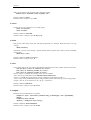
1
DeepView – The Swiss-PdbViewer
User Guide
v. 3.7
http://www.expasy.org/spdbv/
DeepView – Swiss-PdbViewer user guide. Since there was a strong demand for a
printable version of a DeepView user guide, we decided to prepare this manuscript to
complements the documentation and tutorial found on the web site. We are aware that
this user guide is still incomplete in some chapters, there are references missing, etc.
Please help us to make this user guide useful for you: If you find any errors or
inconsistencies, or you don't find an important piece of information, please let us
know.
The DeepView Team
Geneva, 13 September, 2001
GlaxoSmithKline R&D
World Trade Center I
Rte de l'Aéroport 10
1215 Geneva 15, Switzerland
Contents
Preface ...................................................................................................................................................iii
Introduction............................................................................................................................................ 1
I. Overview .......................................................................................................................................... 1
II. Working Environment..................................................................................................................... 1
Installing DeepView ............................................................................................................................... 4
I. Requirements and Installation .......................................................................................................... 4
II. DeepView Directories ..................................................................................................................... 6
STARTING a DeepView Session .......................................................................................................... 9
I. Loading Files .................................................................................................................................... 9
II. Displaying Windows ..................................................................................................................... 10
III. Obtaining Help............................................................................................................................. 11
Ending a DeepView Session ................................................................................................................ 13
I. Saving Data .................................................................................................................................... 13
II. Closing DeepView ........................................................................................................................ 14
Basic DeepView Commands................................................................................................................ 15
I. Using the Toolbar........................................................................................................................... 16
a. Using the tools............................................................................................................................ 17
b. Using the menus......................................................................................................................... 21
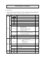
c. Special commands...................................................................................................................... 28
II. Using the Control Panel................................................................................................................ 29
Using the Layers Infos Window......................................................................................................... 34
Advanced DeepView Commands........................................................................................................ 37
I. Working on a Layer........................................................................................................................ 37
a. Modifying commands ................................................................................................................ 38
b. Searching commands ................................................................................................................. 46
c. Computing commands ............................................................................................................... 50
d. Crystallographic commands....................................................................................................... 58
II. Working on a Project .................................................................................................................... 64
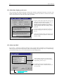
a. Merging commands.................................................................................................................... 67
b. Superposing commands ............................................................................................................. 68
c. Alignment commands ................................................................................................................ 73
Homology Modeling............................................................................................................................. 75
I. Loading Files .................................................................................................................................. 77
II. Generating a Modeling-Project ..................................................................................................... 79
III. Submitting a Modeling-Project.................................................................................................... 83
IV. Evaluating and Improving the Model .......................................................................................... 84
Display Modes ...................................................................................................................................... 85
I. Non Stereoscopic Modes ................................................................................................................ 86
II. Stereoscopic Modes ...................................................................................................................... 88
Setting Preferences .............................................................................................................................. 91
I. Overview ........................................................................................................................................ 91
II. Setting Preferences........................................................................................................................ 92
Annex 1: List of Key Modifiers and Menus..................................................................................... 103
ii
DeepViewManual
I. Key Modifiers............................................................................................................................... 103
II. List of Menus .............................................................................................................................. 104
Annex 2: Scripting Language ........................................................................................................... 110
I. Using Scripts ................................................................................................................................ 110
II. Scripting Language ..................................................................................................................... 110
III. List of Commands...................................................................................................................... 113
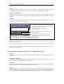
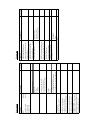
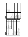
Annex 3: Hardware Requirements................................................................................................... 130
Annex 4: CALCULATIONS ............................................................................................................. 132
I. Connect......................................................................................................................................... 132
II. Secondary structure detection ..................................................................................................... 132
III. Mutations ................................................................................................................................... 132
IV. Building loops............................................................................................................................ 133
V. Molecular surfaces ...................................................................................................................... 133
VI. Electrostatic potentials............................................................................................................... 133
VII. Electron density maps .............................................................................................................. 134
VIII. Solvent accessibility................................................................................................................ 134
IX. Matrices ..................................................................................................................................... 135
X. Threading energy / mean force potential (PP) ............................................................................ 135
XI. FORCE FIELD ENERGY (FF) ................................................................................................. 135
XII. transformation matrices ............................................................................................................ 135
XIII. RMSD ..................................................................................................................................... 135
XIV. Sequence Similarity ................................................................................................................ 135
Annex 5: Glossary .............................................................................................................................. 136
References........................................................................................................................................... 137
Preface
Acknowledgements
The following manual has been prepared by Mercé Ferres in the Protein Structure Bioinformatics group
of GlaxoSmithKline Research and Development S.A., Geneva with contributions from Nicolas Guex,
Alexander Diemand and Torsten Schwede. We would like to thank all our users who have contributed
innumerable suggestions, bug reports and new ideas that let to the development of DeepView – the
Swiss Pdb Viewer in its current form. We are especially grateful to Gale Rhodes (University of Maine),
Simon Andrews (BBRC) and Joe Krahn (NIEHS) for continuously supporting our efforts.
To learn more about molecular modeling and molecular visualization, we would encourage you to refer
to the following Tutorials:
• Gale Rhodes: The Molecular Modeling Tutorial for Beginners
http://www.usm.maine.edu/~rhodes/SPVTut/
• The DeepView advanced tutorial
http://www.expasy.org/spdbv/text/tutorial.htm
Structure of this manual
This manual has been organized in "points" describing certain features or functions of DeepView –
Swiss-PdbViewer. The first chapters describe "simple" operations needed to open and display
molecular structures, while more complex manipulations are provided in later chapters.
DeepView – Swiss-PdbViewer has been designed to work under different operating systems
(Macintosh, Windows, Linux, Irix 6.x), i.e., the commands mentioned in this manual apply to all
versions of the program. However, not all functions using the keyboard could be mapped consistently
between all different OS (e.g. the ALT – CTRL keys). In these cases, this manual will provide a table
of different keyboard-settings.
Legal Disclaimer
The authors reserve the right to change, without notice, the specifications, drawings and information
contained in this manual. While every effort has been made to ensure that the information contained in
this manual is correct, the authors and GlaxoSmithKline Research and Development S.A., Geneva
(herein after called GSK) do not assume responsibility for any errors, which may appear. DeepView –
the Swiss-PdbViewer is provided without warranty of any kind whether express, statutory or implied,
including all implied warranties of merchantability and fitness for a particular purpose.
DeepView – Swiss-PdbViewer is provided on an "as is" basis. The limited license grant means that you
may not do the following with Swiss-PdbViewer: decompile, disassemble, reverse engineer, modify,
lease, loan, sell, distribute or create derivative works based upon the Swiss-PdbViewer software in
whole or in part without written permission of the authors; transmit Swiss-PdbViewer to any person,
except if the original package and its whole original content is transmitted, and that this person accepts
to be bound by the terms and conditions of this software license agreement and warranty.
Neither the authors nor GSK shall in any event be liable for any direct, consequential, incidental,
indirect or special damages even if advised of the possibility of such damages. In particular, the authors
and GSK shall have no liability for any damage loss or corruption of data or programs stored in or used
in conjunction with DeepView – Swiss-PdbViewer, nor shall the authors or GSK be liable for the cost
of retrieving or replacing damaged lost or corrupted data. If for any reason a court of competent
jurisdiction finds any provision of this license to be unenforceable, the other provisions of this limited
warranty and software license agreement shall remain in effect without limitation.
All products mentioned in this user guide are trademarks of their respective companies.
INTRODUCTION
I. OVERVIEW
DeepView – the Swiss-PdbViewer (or SPDBV), is an interactive molecular graphics program for
viewing and analyzing protein and nucleic acid structures. In combination with Swiss-Model (a server
for automated comparative protein modeling maintained at http://www.expasy.org/swissmod) new
protein structures can also be modeled.
Annex 5: Glossary provides an extended dictionary for DeepView terminology. To facilitate
understanding of the following chapters, some essential terms are introduced here:
A molecular coordinate file (e.g. *.pdb, *.mmCIF, etc.) is a text file containing, amongst other
information, the atom coordinates of one or several molecules. It can be opened from a local directory
or imported from a remote server by entering its PDB accession code. The content of one coordinate
file is loaded in one (or more) layers, the first one will be referred to as the "reference layer".
DeepView can simultaneously display several layers, and this constitutes a project. When working on
projects, the layer that is currently governed by the Control Panel is called the currently active layer.
Each molecule is composed of groups, which can be amino acids, hetero-groups, water molecules, etc.
and each group is composed of atoms.
Non-coordinate files containin specific information other than atom coordinates. Molecular surfaces,
electrostatic potential maps, and electron density maps are examples of non-coordinate files, which
can either be computed by DeepView, or loaded from specialized external programs.
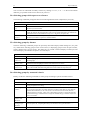
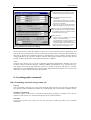
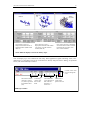
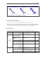
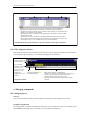
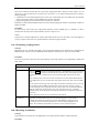
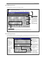
II. WORKING ENVIRONMENT
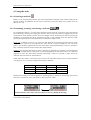
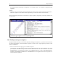
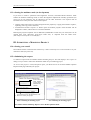
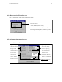
DeepView can display up to eight interconnected interactive windows. This section presents the
general purpose of every DeepView window, each of which will be fully described later.
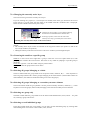
1 ● Graphic window (see 23, 167)
It is used to visualize loaded molecules, which can be rotated, translated and zoomed.
Display of the coordinate axis is optional. Molecular surfaces, electrostatic potential maps, and electron
density maps can also be displayed on the Graphic window.
2 ● Control Panel (see 70)
This table-like window is for controlling the visual representation of the currently active layer.
It lets you enable the display of backbones, side chains, labels, molecular surfaces, and ribbons for each
group; and set the colors for the different objects on display.
3 ● Toolbar (see 38 – 40)
Contains the menus and tools of the program.
DeepViewManual
2
These let you analyze the loaded molecules and use Swiss-Model in combination to model new
structures.
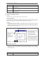
Toolbar
Graphic
window
Main
windows
Specific
windows
Deep View working environment.
4 ● Layers Infos window (see 84)
This table-like window is for controlling the display of individual layers.
You can toggle on and off the visualization and movement of layers, and enable the display of certain
objects (e.g. H-bonds or water molecules), for each layer.
5 ● Alignment window (see 114)
Shows the amino-acid sequence of loaded proteins in one-letter abbreviations.
This window is used to compare and to align sequences of two or more proteins. During homology
modeling, it allows correcting the alignment of target sequences onto the templates.
6 ● Ramachandran Plot window (see 93)
Displays a Ramachandran plot.
Each dot on the plot gives the φ and ϕ angles of one selected residue of the currently active layer.
Ramachandran plots are used to judge the quality of a model, by finding residues whose
conformational angles lie outside allowed regions.
INTRODUCTION
3
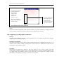
7 ● Surface and Cavities window (see 102)
Gives the surface (Ǻ2) and volume (Ǻ3) of a molecule and its cavities.
This window can only be displayed if a molecular surface has been computed. It is mainly for
information purposes, but can also be used to center the view on specific cavities.
8 ● Electron Density Map Infos window (see 103)
This is a table-like window that lets you control the appearance of electron density maps and
electrostatic potential maps.
9 ● Text windows
In addition to all previously described windows, you can open many Text windows for viewing
text files such as PDB files, energy reports, BLAST results, help texts, etc.
Text files cannot be edited or printed directly in DeepView. Please use any text editor for this purpose.
INSTALLING DEEPVIEW
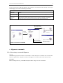
I. REQUIREMENTS AND INSTALLATION
10 ● Requirements
Platform
Required Hardware
Required Operating System
PC
Pentium or 486DX.
Win 95, 98, 2000, NT4
Open GL
Mac
Power Mac (Mac68K are no longer supported).
256 colors monitor.
Extended Keyboard highly recommended.
Open GL
(QuickDraw3D no longer supported)
Linux
US Keyboard.
3 button mouse.
Linux for PC (with glibc-2.0 or higher).
Preferably RedHat
X11R6 with at least 16bits.
MESA libraries.
Irix
02, Octane
IRIX 6.x (preferably 6.5)
(IRIX 5.3 no longer supported).
NOTE:
See ANNEX 3: HARDWARE REQUIREMENTS for hardware stereo support.
11 ● Installing DeepView on PC
DeepView can be downloaded from http://www.expasy.org/spdbv/ or any of the mirror sites
mentioned there.
a) Download & install Swiss-PdbViewer.
DeepView is distributed either as a self extractable archive (.exe) or as a zip archive (.zip):
• (.exe): Double click the file. By default, a directory called spdbv will be created in your C: drive.
You can move this directory where you want on your hard drive. Be sure to maintain the directory
content (see points 15-20). To launch DeepView, double click the application icon ( ).
• (.zip): The file can be expanded using WinZip. In this case, be sure to configure WinZip so as to
keep the directory hierarchy.
The following steps b) – f) are optional.
b) Download Swiss-PdbViewer Loop Database (2.45 Mb).
This step is useful if you intend to do standalone modeling, or for teaching purposes. To be able to use
the loop database, put it into the _stuff_ directory (see point 15).
c) Download the User Guide (740 Kb).
This step is useful if you want to consult this user-guide from a computer not connected to the network.
To be able to consult the help directly from within DeepView, place the content of this folder into the
_stuff_ directory.
d) Download the Tutorial Material (325 Kb).
This step is useful to learn how to use DeepView by looking at real examples.
e) Download PROSITE pattern file (http://www.expasy.org/prosite/)
INSTALLING DEEPVIEW
5
DeepView can search a sequence for PROSITE patterns, if you download the pattern file prosite.dat
into the usrstuff directory.
f) Download and install POV-Ray.
This step is useful only if you intend to make ray-traced images from your molecules.
NOTE:
• OpenGL is included in all current Windows versions. If during installation of DeepView a missing
glu.dll or missing opengl32.dll error message is displayed, this means that OpenGL is not installed
correctly on your system. Please refer to your graphic card manual or ask your graphic card
manufacturer for support. Standard OpenGL DLLs are available from the Microsoft web site
http://www.microsoft.com.
• Windows NT: The DeepView root directory and the tree below must not be write-protected for the
user executing the program because DeepView will create several temp-files during runtime.
12 ● Installing DeepView on Mac
DeepView can be downloaded from http://www.expasy.org/spdbv/ or any of the mirror sites
mentioned there.
a) Download OpenGL from http://www.apple.com/openGL and install it (if it is not yet present on
your system). This step is optional, but allows rendering nice images.
b) Download Swiss-PdbViewer
The following steps are optional.
c) Download Swiss-PdbViewer Loop Database (3.44 Mb).
This step is useful if you intend to do standalone modeling, or for teaching purposes. If you have a
program that can expand *.zip files, you can download the .zip version which is 2.45Mb. To be able to
use the loop database, put it into the _stuff_ directory (see point 15).
d) Download the User Guide (698 Kb).
This step is useful if you want to consult this user-guide from a computer not connected to the network.
To be able to consult the help directly from within Swiss-PdbViewer, place the content of this folder
into the _stuff_ directory.
e) Download the Tutorial Material (512 Kb).
This step is useful to learn how to use DeepView by looking at real examples.
f) Download POV-Ray (http://www.povray.org)
This step is useful only if you intend to make ray-traced images from your molecules.
NOTE:
If your browser starts to display a lot of text instead of prompting you where to save the program, click
on the link during about 2 seconds until a pop-up menu appears. Then choose the option Save link as...
and check that Source is displayed in the pop-up, not Text. Then drag the downloaded archive file onto
Stuffit Expander.
13 ● Installing DeepView on Linux
DeepView can be downloaded from http://www.expasy.org/spdbv/ or any of the mirror sites
mentioned there.
a) Download Swiss-PdbViewer
6
DeepViewManual
b) tar xzf spdbv35-Linux.tar.gz
c) cd SPDBV_DISTRIBUTION
d) ./install.sh
The Linux version is a port of the Macintosh version done using a preliminary release of Latitude for
Linux kindly made available by Metrowerks Inc. We wish to thank Kevin Buetner for his support, and
Greg Galanos for allowing us to release a version of DeepView that makes use of Latitude.
NOTE:
An error might occur in loading shared libraries libMesaGL.so.3 because the newer Mesa now uses
different names for the libraries than those with which DeepView has been linked with. Libraries are
now called libGL.so and libGLU.so instead of libMesaGL.so and libMesaGLU.so.
However, since the new Mesa is completely backward compatible, it should not harm DeepView from
working properly. Therefore, there is no need to install an old Mesa version, and just a little adjustment
is needed. If you can get root access to your Linux box, make the following symbolic links from the
new libraries to the old names:
ln -s /usr/X11R6/lib/libGL.so.1.2.0 /usr/X11R6/lib/libMesaGL.so.3
ln -s /usr/X11R6/lib/libGLU.so.1.2.0 /usr/X11R6/lib/libMesaGLU.so.3
and then run /sbin/ldconfig to make the system remember this changes. (This is assuming that the
libraries are installed under /usr/X11R6/lib. If this is not correct, please adjust the above commands
with the correct location.)
14 ● Installing DeepView on Irix
DeepView can be downloaded from http://www.expasy.org/spdbv/ or any of the mirror sites
mentioned there.
a) Download Swiss-PdbViewer v3.7b2 (stable Beta version, 6.0 Mb)
b) gunzip -c spdbv35-IRIX.tar.gz | tar xf –
c) cd SPDBV_DISTRIBUTION
d) install.sh
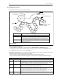
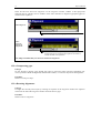
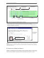
II. DEEPVIEW DIRECTORIES
Depending on whether you installed the optional material or not, the spdbv root-directory will contain
the following directories and subdirectories:
INSTALLING DEEPVIEW
7
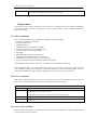
Deep View directories and subdirectories (optional material installed).
15 ● _stuff_ directory
This directory contains files used by DeepView internally, and cannot be altered.
16 ● download directory
Stores all files imported from the server and should be cleared from time to time.
download directory
Files
Description
*.pdb files
PDB and ExPDB files
*.sw files
SWISS-PROT files
*.txt files
Keyword search results, BLAST results, PROSITE documentation, etc.
17 ● scripts directory
Contains scripting examples and a manual for the use of scripts (see Annex 2: Scripting Language)
18 ● temp directory
Stores all files generated by DeepView, such as energy reports (see point 106), PROSITE search results
(see point 99), alignments (see point 121). Although its content is usually cleared when DeepView is
closed, it might be necessary to clear it from time to time.
19 ● tutorial directory
This supplementary directory contains the tutorial and all files needed to run the examples given in the
tutorial.
DeepViewManual
8
20 ● usrstuff directory
This is the “User’s stuff” directory, which stores the settings and the default preferences:
usrstuff directory
Files
Description
recfile.ini:
Contains the five last loaded files
prosite.dat:
Contains all PROSITE patterns. The user has to install this file by retrieving it from the
ExPASy site (http://www.expasy.org/prosite/).
Default.prf
Contains the default preferences (see point 146)
Subdirectory
Description
matrix
Contains all matrices that can be used for sequence alignments, PAM 200 being the
default matrix (see annex 162).
Starting a DeepView Session
Initiating a DeepView session means:
• displaying molecules by loading molecular coordinate files,
• displaying optional objects by loading molecular surfaces, electrostatic potential maps and electron
density maps (molecular surfaces and electrostatic potential maps can also be computed, see points
102 and 103),
• displaying the required windows.
All these actions can be achieved by using the File and Window menus of the Toolbar, as explained in
this chapter.
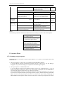
I. LOADING FILES
21 ● Loading molecular coordinate files
The File menu offers the following commands to load a molecular coordinate file. This can be a PDB,
mmCIF, or MOL file:
File menu
Command
Action
Open PDB File
Displays a dialog box that allows loading a PDB file by selecting it.
Open mmcif File
Displays a dialog box that allows loading an mmCIF file.
Open MOL File
Displays a dialog box that allows loading a Molecular Design Limited MolFile (MDL
MolFile).
Import
Displays a dialog box that allows doing one of the following:
1- Retrieving PDB files from a local directory, by typing the molecule accession code and
selecting Grab from disk: PDB File.
NOTE: The path of the local directory, which is the directory in your computer that
contains your own collection of PDB files, needs to be specified (see point 164).
2- Retrieving PDB, SwissProt-sequence and SwissProt-text files via a special DeepView
network server. You achieve this by typing the molecule accession code or its SwissProt
identification and selecting the appropriate button under Grab from server.
NOTE: The network server must be configured (see point 163).
3- Keyword Search for PDB / ExPDB files available on the server using the + (AND) and
– (NOT) connectors. A list of the PDB entries is displayed. To load a file from the given
list, just click its name appearing in red.
If a PDB entry contains more than one chain, several ExPDB file names are available.
Click the right name to load the whole PDB entry (e.g. 1a00), and click the left name to
load just one chain (e.g. 1a00c loads only chain C).
The bottom of the File menu also provides a short list with the five recent files (coordinate and noncoordinate files) that were loaded in previous DeepView sessions.
Other ways to load molecular coordinate files include:
Platform
Load a molecular coordinate file by…
Windows
dragging one or several PDB files onto the Toolbar. Only valid for PDB files.
DeepViewManual
10
Mac
dragging one or several PDB file icons onto the Swiss-PdbViewer icon. Only valid for
PDB files.
Linux and Irix
typing a command line argument, e.g. $>spdbv pdb1.pdb.
NOTE:
Mac, Linux and Irix: These actions launch DeepView and load selected files or, if DeepView is already running,
add selected files into the workspace.
22 ● Loading non-coordinate files
The File menu offers the following commands to load a non-coordinate file:
File menu
Command
Action
Open Text File
Displays a dialog box that allows opening any text file, including scripts. Text files are
displayed in a simple window with a scrollbar. (Shortcut: Ctrl + click
bottom left corner of the Toolbar).
icon in the
Run Script
Displays a dialog box that allows opening and executing a script file. For the use of
scripts see Annex 2: Scripting Language.
Open Surface
Allows loading a molecular surface in three different file formats: the surface might have
been computed and saved from a previous DeepView session (*.sfc) or written by MSMS
[] or GRASP [].
Open Electrostatic
Potential Map
Allows loading an electrostatic potential map in three different file formats: the map
might have been computed and saved from a previous DeepView session (*.sph) or
written by external programs (*.phi).
Open Electron
Density Map
Allows loading electron density maps in either DN6, CCP4, or X-PLOR formats (*.dn6,
*.map, *.txt). []
II. DISPLAYING WINDOWS
For an overview of all DeepView windows see points 1-9.
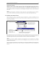
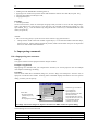
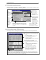
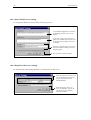
23 ● Initial windows location
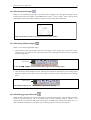
The first time you use DeepView and load a molecular coordinate file, the program opens the Toolbar,
the Graphic window and the Control Panel, as shown on the figure below. When closing DeepView,
the program remembers which windows were open and their locations. So if you already ran the
program, window locations will be those of your previous session. Once a molecule is loaded, use the
Window menu to manage the display of windows.
INITIATING A DEEPVIEW SESSION
11
Toolbar
Layer name and window size (pixels)
Optional
global
axis
Control
Panel
Graphic
window
Initiating a Deep View session: displayed windows and their location.
24 ● Displaying/closing a window
Under the Window menu, click the name of a window to open it or to send it to front. An Electron
Density Map window or a Cavities window can only be displayed if an electron density map or a
molecular surface were loaded (or computed, see point 102). To close a window, follow the normal
procedure of the operating system.
25 ● Linking the Toolbar and the Graphic window
The Toolbar and the Graphic window can be linked, by checking Link Toolbar and Graphic Window
under the Window menu. Both windows will then move together when one of them is moved.
NOTE:
Problems were reported when this option is enabled on some Linux and Irix systems.
26 ● Bringing a Text window to front
Click Window>Text to bring to front the first-loaded Text window.
III. OBTAINING HELP
According to the platform, look under one of the following menus:
Platform
Look under…
Windows
Help menu
Mac
Apple menu
Linux and Irix
Info menu
These menus contain commands that allow:
• obtaining information about DeepView,
• obtaining help in using DeepView,
• updating the program.
DeepViewManual
12
27 ● Obtaining information about DeepView
"About Swiss-PdbViewer" will display the DeepView “splash” screen, with the current version of the
program and a list of authors.
28 ● Obtaining short help about a particular window
Either click its small red question mark, or select the window under the Help, Apple or Info menus
(according to the platform).
29 ● Obtaining detailed help about all DeepView commands
Under the Help, Apple or Info menus (according to the platform), click one of the following commands:
Help, Apple or Info menus (according to the platform)
Command
Action
WWW Manual
Opens your web browser to the HTML User Guide at the DeepView Home Page.
Local Manual
Opens your web browser to the HTML manual stored on your computer, provided that
you have downloaded and installed it in your stuff directory (see point 15).
User Defined Links
Opens your web browser to the page “user.htm” in your usrstuff directory, and lets
you set your favorite links to go quickly where you want on the net, directly from
within DeepView (see point 20).
30 ● Updating the program (not implemented yet)
Under the Help, Apple or Info menus (according to the platform), click Update Swiss-PdbViewer: the
program will look in the server for a new version of DeepView, or for updated library files, and will
automatically download and install them on your computer.
Ending a DeepView Session
During a DeepView session, you might have loaded several molecular coordinate files (see point 21),
displayed objects around them. As DeepView will immediately quit when you invoke the Exit
command (see point 36), before ending your session, you might want to:
• save your data,
• systematically close your files.
These actions can be achieved by using the File menu of the Toolbar.
I. SAVING DATA
Select File>Save: this command offers a submenu to save data and images.
31 ● Saving molecular coordinate files
File>Save command
Subcommand
Action
Layer
Saves the currently active layer in PDB format.
In addition to atom coordinates, saved data include the current Control Panel settings,
the current view orientation, the background color, and any added bonds, except
hydrogen-bonds. The REMARKs (journal references, statistics, etc.) from the
originally opened PDB file are not included. (Other programs should be able to read the
atom coordinates saved in this format, but will ignore the additional information saved
by DeepView).
Project
Saves all layers in a single PDB file (see point 113).
The saved file contains the same data as above. (Other programs should be able to read
the atom coordinates, but will not distinguish the different layers).
Save Selected
Residues
Saves the currently selected groups from all layers to a PDB file.
mmcif
Saves a molecular coordinate file to an mmCIF file. (This format will eventually
replace the current PDB format).
32 ● Saving non-coordinate files
Surface
Saves a surface to a SPDBV surface file (*.sfc).
Electrostatic
Potential
Saves a computed electrostatic potential map to an SPDBV potential file.
Sequence (FASTA)
Saves the sequence of the currently active layer in FASTA format (single letter codes).
Alignment
Saves the current sequence alignment, formatted exactly as seen by clicking the page
icon on the left side of the Align window.
Ramachandran Plot
Values
Saves a simple list of angles for selected residues of the currently active layer. You
must first open the Ramachandran Plot window to calculate the angle values. The file
contains, for each residue, the layer name, the 3-letter residue name, the secondary
structure type ('H', 'S' or ' '), the peptide dihedral bond angle (ω), and the backbone
conformational dihedral angles (φ and ϕ).
DeepViewManual
14
33 ● Saving images
Image
Saves an exact copy of the current Graphic window contents. The format depends on
the platform: Mac saves in PICT format. Windows saves simple files in Bitmap format
(*.bmp) and OpenGL files in Targa format (*.tga). Linux and Irix save in Targa format.
To convert files to other formats, use image file converters, such as convert name.tga
name.tif (Linux and Irix), or Graphic Converter (Mac).
Stereo Image
Saves two images corresponding to the left and right eye view according to the current
stereo settings. The file format depends on the platform, as described above.
POV3 Scene
Saves object data to a POV-Ray formatted file, with options for size, anti-aliasing, and
for making a stereo pair (see point 141).
Linux and Irix: Files are saved in the directory defined in the environment variable
SPDBV_POV_PATH. Pressing the Render button will run POV-Ray and display the
result, provided that POV-Ray is installed. The script defined in the environment
variable SPDBV_POV is executed.
Mega POV scene
Same as above, but with smoother colors for molecular surfaces (see point 141).
II. CLOSING DEEPVIEW
34 ● Closing molecular surfaces, electrostatic potential maps and electron density
maps
Point File>Discard: in the associated submenu select the object to be closed, which will be removed
from the currently active layer. (This step is useful to free some memory after manipulating big
objects.)
35 ● Closing layers
Click File>Close to close only the currently active layer.
Click File>Close All Layers to close all layers at once. This command is only active if you are working
on a project (several layers were loaded).
36 ● Closing the program
Click File>Exit to quit DeepView. The next time you use DeepView, the program will remember
which windows were open and their locations.
Note that DeepView never asks if you want to save changes in files or projects before closing them, nor
before quitting the program.
Basic DeepView Commands
37 ● Classification
The following basic DeepView commands are mainly for setting the visualization of molecules by
selecting, displaying, and coloring objects, as well as for analyzing molecules by measuring distances
and angles between atoms. They can be grouped according to their location:
Command
Tools
Location
Edit commands
Select commands
Menus
Toolbar
Display commands
First column
Special
Color commands
Header
Control
Panel
(…
A h ALA 22
…)
Header
See point
Center the visible groups
41
Translate, zoom, and rotate molecules
42
Measure distances between atoms
43
Measure bond angles
44
Measure dihedral angles
45
Identify groups and atoms
46
Display/select groups within a distance of a picked atom
47
Center the model on a picked atom
48
Edit the identification of a molecule
49
- apply basic selections
- select groups by type
- select groups by property
- select groups by secondary structure
- select groups with respect to a reference
- select groups by distance
- select groups by structural criteria
- show/hide various objects
- select various views for displaying a molecule
- set the style of labels placed by the Control Panel
- clear all labels placed by the tools
50
51
52
53
54
55
56
57-58
59
60
61
Let you color all or parts of a molecule by different criteria
62-66
Displays PDB files or opens text files (Ctrl clicking)
67-68
Provides help on the Toolbar
69
Let you center the model on a specific group
Let you select: - all groups belonging to a chain
- all groups belonging to a secondary structure
element
- one single group
- several individual groups
- an interval of groups
72
73
74
75
76
77
show/side/labl/ribn
Toggle the display of groups
78-79
::
Toggle the display of surfaces
80
col
Lets you color a molecule and associated graphic objects
(ribbon, surfaces)
81
vis/mov
Layers
Infos
window
Action achieved
Toggles on and off the display and movement of layers
82
Provides help on the Control Panel
83
Manages the display of projects
85
Provides help on the Layers Infos window
86
16
DeepViewManual
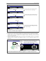
I. USING THE TOOLBAR
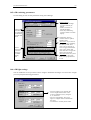
38 ● The Toolbar
The Toolbar contains the tool buttons and menus of the program:
Menus
Tools
PDB file icon: click it to Message space: this is for providing
display the PDB file of
instructions for the use of the tools, as
the currently active layer. well as for displaying information.
Help icon: click it to obtain
help on the Toolbar.
Toolbar: contains the menus and tools of the program.
39 ● The tools
Tools for basic
functions.
1
2
3
4
5
6
Tools for advanced
functions.
7
8
9
10
11
12
13
A active tool appears in
inverse video.
Deep View tools.
A tool is selected by clicking its icons. To deselect tools 2 to 10, either select another tool or press Esc to
activate the rotation tool.
For explanations on tools 11, 12, and 13 (which are for achieving advanced function) see points, 117, 88,
and 89, respectively.
Tools 5 to 8 add labels on the Graphic window. To remove those labels see point 61.
40 ● The menus
Menus containing commands
for basic functions.
Menu for initiating
/ending a session.
Menus containing commands
for advanced functions.
Menu for setting
preferences.
Menu for
homology
modeling.
Menus for getting
help and displaying
windows.
BASIC DEEPVIEW COMMANDS
17
a. Using the tools
41 ● Centering a molecule
Button 1 is for centering the molecule: this will be automatically adjusted so that visible residues fit the
Graphic window. All platforms can also center a molecule by using the "Home" key (oblique arrow on
Mac) or the = key.
42 ● Translating, zooming, and rotating a molecule
For all platforms, buttons 2, 3, and 4 control movement of the molecule. From left to right, these buttons
allow translating, zooming, and rotating the molecule. The currently active button is mapped onto the left
mouse button. On the Graphic window, the cursor changes to show which button is selected. Pressing tab
repeatedly cycles through the three commands from left to right. Holding down the Shift key while
pressing tab repeatedly cycles through the three commands from right to left.
Linux, Irix: in addition to buttons 2 to 4, the left, mid, and right mouse buttons provide rotation, zoom,
and translation, respectively, provided that the rotate button is selected (mapped on the left mouse
button). It is therefore suggested to leave the rotate button selected permanently, so that it is possible to
fully control the molecule motion with the three mouse buttons.
Windows: use the left mouse button to rotate a molecule, the right button to translate it, and both buttons
to zoom it, provided that the rotate button is selected (mapped on the left mouse button). It is therefore
suggested to leave the rotate button selected permanently, so that it is possible to fully control the
molecule motion with the two mouse buttons.
When either the translate or the rotate tools are active, the selected movement can be constrained about
or along the X, Y, or Z axes by using the following key modifiers:
Platform
X
Y
Z
Windows
F5
F6
F7
Mac
Control
Option
Command
Linux and Irix
Control
Alt
Alt+Control
Rotation and translation can also be applied to selected groups by clicking on the message space below
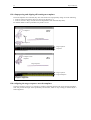
the tools, to switch from “Move All” mode to “Move Selection” mode:
Switch from Move All to Move Selection, and vice-versa, by clicking the message.
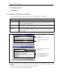
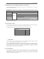
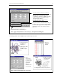
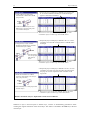
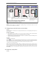
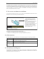
Depending on whether the Move Selection mode or Move All mode is selected, the atom coordinates of a
moved layer will be altered:
18
DeepViewManual
Original structure.
X, Y, Z coordinates of the first seven
atoms of the original PDB file (to
display a PDB file see point 67).
2- Select File>Save>Layer to save the translated structure (see
point 31).
Move All mode
1- Translate the
structure using
the Translate
tool.
3- Open the translated structure again and
display its PDB file: the X, Y, Z atom
coordinates did not change.
Move Selection mode
1- Select all
residues (see
point 50), and
translate the
whole structure
using the
Translate tool.
2- Select File>Save>Layer to save the translated structure (see
point 31).
3- Open the translated structure again and
display its PDB file: the X, Y, Z atom
coordinates did change.
Move All vs. Move Selection modes: implications on the atom coordinates.
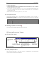
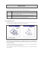
43 ● Measuring distances between atoms
Buttons 5 is for measuring distances between atoms. Click the button, and follow the instructions that
appear in the message space below the toolbar (1. Pick 1st atom; 2. Pick 2nd atom). After you have picked
two atoms on the molecule, the distance is shown as a label, along with a dotted line:
1
2
Distance measured between two atoms picked on the Graphic window.
BASIC DEEPVIEW COMMANDS
19
44 ● Measuring bond angles
Button 6 is for measuring bond angles. Click the button, and follow the instructions that appear in the
message space below the toolbar (1. Pick center atom; 2. Pick 2nd atom; 3. Pick 3rd atom). After you have
picked three atoms on the model, the angle is shown as a label, along with a dotted line.
2
1
3
Angle measured between three atoms picked on the Graphic window.
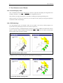
45 ● Measuring dihedral angles
Button 7 is for measuring dihedral angles.
• Click the button and, following the instructions that appear in the message space below the toolbar,
pick one atom. The values for ω, φ, and ϕ of the amino acid containing the selected atom are displayed
on the message space.
Selected tool
Values for ω, φ, and ϕ of a selected amino acid are given on the message space.
• Click the button while holding Ctrl and, following the instructions that appear in the message space
below the toolbar, pick 4 atoms. The torsion angle of the four atoms is displayed on the message
space.
Selected tool
The dihedral angle of four selected atoms is given on the message
46 ● Identifying groups and atoms
Button 8 allows identifying an atom and the group to which the atom belongs. Click the button and pick
one atom. The atom type (CA, CB, O…) and the group to which it belongs (LYS116, ASN117…) are
displayed both on the molecule and on the message space. In addition, the message space gives the x, y, z
atom coordinates and B-factor. (For further ways to label groups on a molecule, see point 78.)
20
DeepViewManual
Identification of an atom picked on the Graphic window.
Selected tool.
layer
name
amino atom
acid
type
x, y, z atom
coordinates
atom
B-factor
Identification of the same atom on the Toolbar.
47 ● Displaying/selecting groups within a distance of a picked atom
Button 9 allows restricting the display of the molecule on the Graphic window, or the selection of amino
acids on the Control Panel, to groups within a distance of a picked atom. Click the button and, following
the instructions that appear in the message space below the toolbar, pick one atom. The Display Radius
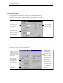
dialog box allows entering a distance and choose one of the following options:
- Adds to a previous display those groups that are
within the entered distance of the picked atom.
- Displays groups on the Graphic window that are
within the entered distance of the picked atom.
- Selects groups on the Control Panel window that
are within the entered distance of the picked atom,
- Adds to a previous selection those groups that are
within the entered distance of the picked atom.
Enter here the distance.
If more than one layer was loaded, the Display
Radius dialog box lets you enable/disable
application of the tool to all layers.
Display Radius dialog box.
48 ● Centering the view on a picked atom
Button 10 is for centering the display of a molecule on a selected atom. Click the button and pick one
atom. The display jumps to center the molecule on the picked atom. (For centering a molecule on a
specific group by using the Control Panel, see point 72).
BASIC DEEPVIEW COMMANDS
21
b. Using the menus
Edit menu
49 ● Editing the identification of a molecule
The Edit menu offers three commands that allow editing the identification of a molecule:
Edit menu
Command
Action
Rename Current
Layer
Displays the Rename Layer Components dialog box, which allows renaming the currently
active layer, and changing the chain identifier of selected amino acids as well as
renumbering them (see figure below).
Rename Selected
HETATMs
Displays the Rename HETATMs dialog box, which allows renaming selected hetero groups
as well as their atom names (see figure below).
Fix Atoms
Nomenclature
Checks if amino acids atom names are conform to the IUAPAC standard. This is useful
since files returned from Swiss-Model (see chapter on homology modeling), or files that
have been energy minimized with external force fields (see point 107), sometimes contain
wrong atom names.
Fields for renaming:
- the layer,
- the chain ID of selected groups.
Field for renumbering selected
groups.
Field for renaming the selected
HETATM.
Field for renumbering the
atoms belonging to the selected
HETATM (four characters per
atom, as in PDB files).
Rename Layer Components and Rename HETATMs dialog boxes.
In addition to these specific commands, the Edit menu includes the following commonly used
commands:
• Undo and Redo, which allow undoing and redoing the last action,
• Cut, Copy, Paste, and Clear (not implemented yet).
22
DeepViewManual
For explanations on all other commands of the Edit menu (which consist of advanced commands) refer to
the following points:
Edit menu
Command
Script Commands
See point
Annex 2: Scripting
Language
Find Sequence
98
Find Next
98
Search for PROSITE pattern
99
BLAST selection vs. SwissProt
100
BLAST selection vs. ExPDB
100
Assign helix-type to selected aa
Assign strand-type to selected aa
97
Assign coil-type to selected aa
Select menu
The Select menu allows selecting specific groups on the Control Panel on the basis of atom properties,
residue properties, structure properties, or other criteria. Selected groups appear in red on the Control
Panel.
If several layers are loaded, shift-clicking a Select option allows extending the selection to all layers.
50 ● Applying basic selections
Use the following commands of the Select menu to achieve the following basic selections:
Select menu
Command
Action
All
Selects all groups.
None
Deselect all groups.
Inverse Selection
Selects the inverse of a current selection.
Visible groups
Selects those groups for which the backbone, the ribbon, or both, are displayed on the
Graphic window.
Pick on screen
Allows selecting groups by picking them on the Graphic window.
Extend to other
layers
When working on a project, this command copies selection status from groups in the
currently active layer to all other layers, based on the sequence alignment. This command is
useful for identifying important counterpart residues for an aligned structure, such as active
site residues.
Groups with same
color as
Allows picking a residue on the Graphic window, and selects all residues with the same
color.
BASIC DEEPVIEW COMMANDS
23
51 ● Selecting groups by type
Click Select>Group Kind. This displays a submenu to select groups by type:
Select>Group Kind command
Subcommand
Groups selected
Ala (A)
[...]
Val (V)
All residues of the choosen type.
G, A, T, C, U
All nucleotides of the choosen type. Non standard nucleotides cannot be recognised, instead,
they can be selected as hetero-groups.
HETATM
All groups defined as a hetero-group.
Solvent
All water molecules, i.e. groups named WAT, SOL, HOH or H2O.
(NOTE: Water molecules are not loaded by default. To load them, disable Ignore Solvent in
the Loading Molecule Preferences dialog box, see point 150).
SS-bonds
Identified Cys-Cys disulfide bonds.
52 ● Selecting groups by property
Click Select>Group Property. A submenu lets you select amino-acids according to four property
categories. It is currently not possible to change which residue belongs to which category, but scripting
commands can be used to add a menu that define your own selections (seeAnnex 2: Scripting Language).
Select>Group Property command
Subcommand
Groups selected
Basic
Arg, Lys, His
Acidic
Asp, Glu
Polar
Asn, Gln, Ser, Thr, Tyr
non-Polar
Ala, Cys, Gly, Ile, Leu, Met, Phe, Pro, Trp, Val
53 ● Selecting groups by secondary structure
Click Select>Secondary Structure. A submenu lets you select all residues that belong to a standard
secondary structure type, or all amino acids that verify a specific main-chain property.
Select>Secondary Structure command
Subcommand
Groups selected
Helices
All residues of any helix ("h" in Control Panel window).
Strands
All residues of any strand ("s" in Control Panel window).
Coils
All residues of any coil between two specific secondary structure elements (" " in Control
Panel window). Even non-amino acid groups are selected.
non-TRANS aa
Residues with cis- or distorted peptide bonds.
aa with Phi/Psi out
of Core Regions
Residues outside of the common α, β, and αL core regions (see point 93, Ramachandran
Plot, []).
aa with Phi/Psi out
of Allowed Regions
Residues with unusual φ and/or ϕ values. Few residues should be here, except for Gly (see
point 93, Ramachandran Plot, []).
NOTE:
24
DeepViewManual
You can select an individual secondary structure by clicking on a "h", "s" or " " in the second column
under the group header of the Control Panel (see point 74).
54 ● Selecting groups with respect to a reference
The following commands presuppose that a structural alignment has been computed (see point 121):
Select menu
Command
Action
aa identical to
ref.
Selects residues that are strictly conserved between the currently active layer and the
reference layer (first loaded).
aa similar to ref.
Selects similar residues between the currently active layer and the reference layer (first
loaded). By default, the PAM 200 matrix will be used, and the minimum score needed to be
considered similar can be modified in Preferences>Alignment (see point 162).
aa matching ref.
structure
Selects residues of the currently active layer whose backbone has a RMS deviation to the
reference layer inferior or equal to a certain threshold.
55 ● Selecting groups by distance
The three following commands prompt the previously described Display Radius dialog box (see point
47), which allows selecting groups on the Control Panel, or displaying groups on the Graphic window,
within a distance that you can specify. The dialog lets you extend a selection/display around a previous
selection/display, and includes an option to act on all layers.
Select menu
Command
Action
Neighbors of
selected aa
Selects/displays groups with at least one atom within the specified distance of any atom of
selected groups.
Groups close to
another chain
Selects/displays any group that is near any other group with a different chain ID. This
command is useful to highlight residues at the interface of two chains.
Groups close to
another layer
Selects/displays any group that is near any other group from a different layer. It applies to all
layers, and is useful when interacting chains have been loaded into separate layers.
56 ● Selecting groups by structural criteria
Finally, use the five following commands to select groups according to specific structural criteria.
Select menu
Command
Action
Accessible aa
Selects residues with an accessible surface area higher than a given percentage, which you
will be prompted for in a dialog.
aa Making
Clashes
Selects residues with atoms too close to atoms of other residues. Since van der Waals radii
are not assigned when files are loaded, DeepView looks for atoms that are closer than the
minimal H-bond distance (as set in Preferences>H bond detection threshold, when no
hydrogen atoms are present). A finer way to find clashes consists in coloring the molecule
by force field energy: residues that have a high non-bonded energy (colored in red) are too
close to each other.
aa Making
Clashes with
Backbone
Selects groups with at least one atom too close to the backbone of another group.
Sidechains
lacking Proper
H-bonds
Selects those buried residues whose sidechain could make an H-bond or a salt-bridge, but do
none (see point 101, computing H-bonds]). Few should occur in good structures.
Reconstructed
Selects residues with reconstructed sidechains. These may have been built automatically for
BASIC DEEPVIEW COMMANDS
amino-acids
25
residues with missing atoms, which often occurs for highly mobile surface residues.
Automatic reconstruction can be disabled (see point 149).
Display menu
The Display menu is mainly comprised of Show and View commands. These are checkbox commands,
which turn on and off various viewing options. Some of these options are also available through the
Layer Infos window.
57 ● Show commands
Show commands consist of self-explanatory toggles for showing or hiding:
• the global coordinate system axes,
• the carbon alpha trace,
• backbone oxygens,
• sidechains even when backbone is hidden,
• dot surfaces (must have been computed first),
• forces (must have been computed first),
• hydrogens,
• H-bonds (must have been computed first),
• H-bond distances (must have been calculated),
• H-bonds from selection (must have been computed),
• groups with visible H-bonds (H-bonds must have been built).
To compute H-bonds, surfaces, and forces, see points 101, 102, and 106, respectively.
Show commands apply only to the currently active layer, except for Show Axis, since all layers use the
same coordinate system. To extend a Show command to all layers, select it while holding Shift. The most
used Show commands are readily available through the Layers Infos window (see point 85).
58 ● Views command
This offers a submenu that allows saving a view, reseting a previous view, and deleting a saved view. A
view of a molecule is defined by the orientation and perspective of the molecule.
Display>Views command
Subcommand
Action
Save
Prompts a dialog that lets you name a view to save it. The name of the saved view is then
included in the last line of the submenu.
NOTE: When saving a layer, all saved views are stored with the layer.
Reset
Displays the original model view, when first loaded.
Delete
Prompts a message reminding how to delete a saved view, i.e. by selecting it while holding
down Ctrl.
59 ● View From command
Allows rotating the molecule to change the point of view. This command is no longer maintained and
will be removed in future versions.
26
DeepViewManual
60 ● Setting the style of the labels placed with the Control Panel
Labels for individual groups can be placed by using the tools, as explained above, or by using the
Control Panel (see points 78-79).
Click Display>Label Kind and select a submenu to set the display of the labels placed by using the
Control Panel:
Display>Label Kind command
Subcommand
Action
Group Name
Group name, e.g. LEU125.
Atom Name
Atom name, e.g. CA, C, O, N.
Atom Type
Atom Charge
Set the label
style by:
Atom type, e.g. C, C, O, N.
Atom charge, e.g. 0.000, 0.380, - 0.380, - 0.280. Only valid after an energy
computation has been made.
Atom code, referring to the GROMOS96 force field, e.g. 12, 11, 1, 5. Only
valid after an energy computation has been made.
Atom Code
(GROMOS 96)
Selection will apply to all layers.
61 ● Clearing user’s labels
Click Display>Label Kind>Clear User Labels to clear any label added to the molecule by using the
tools. Labels added by using the Control Panel will not be cleared (see point 78).
For explanations on all other commands of the Display menu, refer to the given points:
Display menu
Command
Slab
Stereo view
See point
138
142-144
Use OpenGL Rendering
140
Render in solid 3D
140
Color menu
The Color menu is used to systematically apply colors to the Backbone, Sidechain, Ribbon, Label, and
Surface of each group. Backbone & Sidechains can be colored at once.
Look at the first line of the Color menu. This indicates what object (Backbone + Sidechain, Backbone,
Sidechain, Ribbon, Label, or Surface) will be colored by the subsequent coloring operations. The object
can be selected by using the pop-up menu associated to this command, or by using the pop-up menu
under the header col of the Control Panel (see point 81).
62 ● Coloring objects
Use one of the Color menu functions (63) to color the selected object. If a Color command is invoked
while holding down the Shift key, colors are appplied to all layers. If a Color command is invoked while
holding down the Ctrl key, only selected groups are colored (currently this works only when selecting
Color>by CPK or Color>by Other Color).
BASIC DEEPVIEW COMMANDS
27
63 ● Color menu, first block
Color menu
Command
Coloring action
By CPK
Colors the selected object by element type, using a default standard CPK scheme: N=blue,
O=red, C=white, H=cyan, P=orange, S=yellow, other=gray. This command is only effective
if backbones and/or sidechains are selected for coloring. Default colors can be redefined in
Preferences>Colors (see point 154)
By Type
Colors the selected object by residue property: Acidic=red, Basic=blue, Polar=yellow, and
Non-Polar=gray (Acidic, Basic, Polar, and Non-Polar). Default colors can be redefined in
Preferences>Colors (see point 154).
By RMS
At least two proteins must have been loaded, superposed, and structurally aligned (see points
127-132). Each residue in the active layer will be colored accordingly to its RMS backbone
deviation from the corresponding amino acid of the reference protein (the first loaded).
NOTE: Colors are mapped from a fixed linear scale, in which dark blue is for RMS = 0 Å,
and red is for RMS = 5 Å. A relative scale can be selected in Preferences>General where the
best fit is dark blue and the worst fit is red.
By B-Factor
Colors sidechains and backbones, independently, according to their respective largest B2
factor per group. A color gradient is used in which blue is for B-factor = 0 Å , green is for B2
2
factor = 50 Å , and red is for B-factor ≥ 100 Å .
Ribbons take the colors of sidechains, and surfaces take the color of the B-factor of the
nearest atom.
In the case of a model returned by Swiss-Model, the B-factor column contains the Model
Confidence Factor (see point 135).
NOTE: The coloring gradient can be adjusted in Preferences>General to fit the range of Bfactor values present in the structure (see point 149).
By Secondary
Structure
Colors the selected object according to the three common secondary structure types:
Helix=red, Strand=yellow, and Coil =gray. Especially useful for coloring ribbon drawings.
Default colors can be redefined in Preferences>Colors (see point 154).
By Secondary
Struct. Success.
Produces a gradient along the polypeptide chain from N-terminus (blue) to the C-terminus
(red). Each secondary structure element gets a single color, and random-coils are gray.
Especially useful for coloring ribbon drawings.
64 ● Color menu, second block
Color menu
Command
Coloring action
By Selection
Colors selected residues in cyan and non-selected residues in dark gray. Useful to quickly find
where selected residues are located in the model. Default colors can be redefined in
Preferences>Colors (see point 154).
By Layer
Each layer gets a single unique color. The layers are colored in order from the first as: yellow,
blue, green, red, gray, magenta, cyan, salmon, purple, light green, and brown. The color
succession is repeated for additional layers. Ideal for viewing superposed structures.
By Chain
Colors each chain by a different color: yellow, blue, green, red, gray, magenta, cyan, salmon,
purple, light green, and brown. The color succession is repeated for additional chains.
NOTE: Chains are defined in the PDB file; a break in the modeled polypeptide chain does not
signify a new chain.
28
DeepViewManual
65 ● Color menu, third block
Color menu
Command
Coloring action
By Alignment
Diversity
At least two proteins must have been loaded, superposed, and structurally aligned (see points
127-132). Applies a blue-to-red color gradient to all layers, according to the degree of
similarity among all aligned residues. Blue indicates identical or very similar, and red
indicates that residues have dissimilar properties (see Annex 4: ).
By Accessibility
Each group is colored by its relative accessibility (see Annex 4: ). Colors range from dark
blue for completely buried amino acids, to red for residues with at least 75% of their
maximum surface exposure. The relative accessibility of a residue X is obtained by
comparison to a reference value of 100% accessibility computed in an extended conformation
in the pentapeptide GGXGG.
By Threading
Energy
Colors each residue of the protein according to its energy (computed by a "Sippl-like" mean
force potential, see Annex 4: , []). Dark blue means that the threading energy is low (the
residue is happy with its environment), red means that the threading energy is high (the
residue is not happy with its environment).
By Force Field
Energy
Colors each residue according to its force field energy (computed with a partial
implementation of the GROMOS 96 []). A dialog lets you choose what kind of interaction
you want to compute (bond, angles, improper, electrostatic...) and ask for a text report where
detailed energy of each residue is given. Especially useful during refinement of a model as
you can color by bond and angle deviations only, and this will identify distorted parts of the
protein.
By Protein
Problems
The backbone of those residues whose φ, ϕ angles do not plot in the allowed area of the
Ramachandran Plot is colored in yellow. The backbone of proline residues whose φ angle
deviates more than 25° from the ideal –65° value is colored in red. Buried sidechains of
residues that could make H-bonds but do not are colored in orange. Clashes are computed and
will appear as pink dotted lines.
66 ● Color menu, fourth block
Color menu
Command
Coloring action
By Other Color
Prompts you for a single color to be applied to the entire layer. It is functionally equivalent to
a shift-click on any color box of the Control Panel window (see point 81).
By Backbone,
Sidechain,
Ribbon, Surface,
Label Color
These last five commands are used to copy the current colors set for one object selected here
to the object shown in the first line of the Color menu. Use this to save a set of colors in a
property you're not using (like surface color) and copy it back later.
NOTES:
• Color by CPK is the only coloring command that uses different colors for the different atoms that belong to a
group.
• For colors by CPK, by type, and by secondary structure, default colors can be redefined in
Preferences>Colors (see point 154).
c. Special commands
67 ● Viewing PDB files
BASIC DEEPVIEW COMMANDS
29
Click the dog-eared page icon to open a text window with the content of the original molecular
coordinate file of the currently active layer.
68 ● Navigating in text files Ctrl+
Control clicking the dog-eared page icon opens the Select a TEXT file dialog to let you open any text file.
Very large files are supported, which can be visualized this way.
Many text file elements can be treated as active hyperlinks. When they are clicked they produce an
action, for example:
• Clicking a SWISS-PROT, PDB or PROSITE accession number (which appear in red in text files)
downloads the corresponding file automatically.
• Clicking an ATOM line will center the view of the model on this atom and will display only those
residues that are within a certain radius of the atom. To edit this radius, see point 167.
• Clicking any other line containing the identification of a residue (group name and group number) will
center the view on the carbon alpha of the residue.
NOTE: Text files cannot be edited or printed within DeepView.
69 ● Obtaining help on the Toolbar
Click the small red question mark to obtain help on the Toolbar.
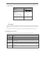
II. USING THE CONTROL PANEL
70 ● The Control Panel
Currently active layer.
List of the groups of the
currently active layer.
Groups identification include:
- protein chain (A, B, etc.),
- secondary structure (h, s)
- group name (SER, GLU, etc)
- group number.
Control Panel.
Control Panel header:
- The first line is for toggling on
and off the visualization and
movement of the currently
active layer, and for getting help
on the Control Panel.
- The second line provides a
series of items to be checked for
viewing them on display, from
left to right: the residue (show),
its sidechain (side), its label
(labl), its molecular surfaces
(::), and its ribbon (ribn). The
last column (col) is for setting
the color for each of these
objects.
These two small black arrows are
for displaying pop-up menus:
- For selecting a surface type (v
in the example, i.e. van der
Waals, see point 80),
- For selecting the object to be
colored (R in the example, i.e.
ribbon, see point 81).
30
DeepViewManual
71 ● Changing the currently active layer
The Control Panel governs the currently active layer.
If you are working on a project (i.e., several layers are loaded), click on the gray bar below the Control
Panel title bar: a pop-up menu with the names of all loaded molecular coordinate files is displayed.
Select one file to make it the currently active layer:
Click the gray bar to display a pop up menu containing
the names of all loaded molecular coordinate files.
On the pop up menu, select a file: this will be the
currently active layer, governed by the Control Panel.
Selecting the currently active layer on the Control Panel.
NOTES:
• The currently active layer can also be selected on the Alignment window (see point 114) and on the
Layers Infos window (see point 84).
• Hitting the Tab key while the Control Panel is the active window cycles through all layers.
72 ● Centering the model on a specific group
Windows: in the Control Panel right-click a group to center the view on its alpha carbon (CA). The
group appears in bold in the Control Panel. This action is very useful for jumping to a specific group in
the model.
Linux, Irix: right Alt + click the residue using any mouse button.
Mac: option-click the group in the Control Panel.
73 ● Selecting all groups belonging to a chain
The first column under the group header is for the protein chains, named A, B, C…. Click anywhere to
select all groups (amino-acids + hetero groups) belonging to the selected chain. (If the model contains no
chain identifiers, the column is blank and clicking it will select all groups).
74 ● Selecting all groups belonging to a secondary structure element
The second column under the group header is for the protein secondary structures, named h, s, (-). Click
anywhere to select all groups (amino-acids) belonging to the selected secondary structure element.
75 ● Selecting one group only
The third column under the group header is for the amino-acids identification (VAL1, LEU2… see point
46). Clicking a group will select it.
76 ● Selecting several individual groups
In the third column under the group header, you can select several individual groups by clicking them
while holding down Ctrl on PCs or Alt on Mac, Linux, and Irix.
BASIC DEEPVIEW COMMANDS
31
Alternatively, you can use the numerical keypad (not implemented yet):
• enter the first group number and then,
• typing + before the next entered number will add the residue to the selection,
• typing - before the next entered number will deselect the residue to the selection.
(e.g. 72+85 will select groups 72 and 85. Typing +87 will add group 87 to the selection, whereas typing –
72 will deselect group 72).
77 ● Selecting an interval of groups
Select an interval of groups by:
• clicking the first group and dragging up or down to the last group,
• clicking the first group and pressing Shift while clicking the last group,
• using the numerical keypad (not implemented yet): enter the number of the first group, type slash, and
enter the number of the last group (e.g. 72/85 will select groups 72 to 85).
NOTES:
• Selected groups appear red in the Control Panel, and the total number of selected groups is displayed
in the Layer Infos window (see point 84).
• For further ways to select groups, see points 50-56.
78 ● Setting the display of a single group
Check/uncheck the columns after the name of a group to display/hide the following objects:
Column
Displayed object for amino-acids
Displayed object for other groups
(Control Panel)
(Graphic window)
(Graphic window)
show
Backbone (*)
Atom or group of atoms
The show column has to be checked to
enable the display of sidechains, labels
and surfaces.
The show column has to be checked to
enable the display of all other checked
options.
side
Sidechain
(no effect)
ribn
Ribbon
(no effect)
labl
Amino-acid label. See point 60 to select
the kind of label.
Group label
NOTE:
(*) In principle, to see the sidechain of a group, its backbone must be displayed. However, see point 57 to
see sidechains without backbone.
79 ● Setting the display of several selected groups
Once you have selected several groups in the Control Panel window, you can:
• press Return to hide unselected groups on the Graphic window,
• set the display of all selected groups at once by checking the Control Panel options as it follows:
All platforms
Left-click
Shift-Left-click
Click any point in a column
Checks/unchecks the pointed group
Checks/unchecks all groups
Click the column header
Checks selected (red) groups only
Checks selected (red) groups only
If several layers are opened, you can extend your check to all layers by:
Mac, Windows, Irix: Shift + Ctrl click.
Linux: shift + left Alt click.
32
DeepViewManual
80 ● Displaying surfaces
DeepView offers three ways to represent a surface:
Accessible surface
Rolling solvent
molecule
R ~ 1.4
Molecular surface
Å
Van der Waals
surface
Molecule
Surface
Definition
Van der Waals
Contact surface of each atom, based on the Van der Waals radius.
Accessible
Surface described by the center position of a water molecule that would
be rolled over the protein. This is approximated by rolling a sphere with
a 1.4 Å radius, which is approximately the radius of a water molecule.
Molecular
Area that can be reached with the surface of a solvent molecule (1.4 Å)
rolled over the protein.
Surface types.
You can display a surface by:
• Directly enabling its display on the Control Panel: van der Waals and Accessible surfaces.
• Computing it first (see point 102) and enabling its display on the Control Panel: Molecular surface.
• Loading it from a file (see point 22): any surface.
Using the Control Panel lets you toggle on and off the display of the van der Waals, Accessible and
Molecular surfaces assigned to each group, individually:
• select a surface in the pop-up menu associated to the surface header (fifth header),
• under the surface header, checkmark the groups for which you want to display the selected surface:
Control Panel, surface header
Header
Surface type
Drawing result
::
v
Van der Waals
A dotted sphere surrounding each atom. The surface will appear as a solid atom when
OpenGL Rendering is enabled, or during POV-Ray renderings (see points 140-141).
The density of points can be set in Preferences>Display (see point 167).
::
a
Accessible
Equivalent to plotting the van der Waals surface increased by 1.4 Å. The density of
points can be set in Preferences>Display (see point 167).
::
m
Molecular
::
u
User
Equivalent to applying a shrink-wrap to the van der Waals surface model.
To display a molecular surface, this must first be computed by clicking
Tools>Compute Molecular Surface (see point 102). The surface quality and its initial
appearance can be modified in Preferences>Surfaces (see point 156)
Not implemented yet.
BASIC DEEPVIEW COMMANDS
33
Accessible
surface.
Van der Waals
surface.
Normal display
Molecular
surface.
Accessible
surface.
Van der Waals
surface.
3D rendering
Molecular
surface.
Normal display
3D rendering
Visualization of Van der Waals, accessible, and molecular surfaces.
81 ● Coloring the molecule
The col column of the Control Panel allows assigning different colors to the backbone(s), side chains,
ribbon(s), labels and surfaces of individual groups:
To select the object to be colored:
In the pop-up menu of the col header select the object to be colored (i.e. backbone, side chains, etc.) in
the next operation:
Control Panel, color header
Header
Selected object
Col
BS
backbone + side (i.e. backbone + side chains)
Col
B
backbone
Col
S
side (i.e. sidechains)
Col
R
ribbon
Col
L
label
Col
U
surface: only valid for molecular surfaces, since van
der Waals and accessible surfaces will always take the
color set for the corresponding atom.
34
DeepViewManual
To color the selected object:
• in the col column select the boxes corresponding to the groups for which you want to color the
selected object. You can either drag your mouse to select several boxes in a row, or shift-click
anywhere in the column to select all boxes.
• a Color dialog is displayed, in which you can select a color. To select the CPK colors hit OK. Notice
that the Cancel button does not work: it colors selected residues black. This action can be annulled by
selecting Color>By CPK.
(For other ways to color a molecule see points 62-66, Color menu).
82 ● Viewing/moving a layer
The following commands, which are only meaningful when working with projects (see chapter on
advanced functions, section B), are located above the column headers of the Control Panel. Check them
to enable the following actions:
Control Panel, upper header
Command
Action
visible
Show/hide the whole layer.
can move
Allows moving the layer (i.e., translating and rotating it).
83 ● Obtaining help on the Control Panel
Click on the red question mark to obtain help on the Control Panel.
III. USING THE LAYERS INFOS WINDOW
84 ● The Layers Infos window
Click the question mark
to obtain help on this
window.
List of all loaded files. The
currently active layer appears
in red. You can select it here.
Layers Infos window
For each layer, check/uncheck
these items to toggle on/off the
display or actions described below.
Hold down Shift to act on all
layers.
Shows the number of
currently selected
groups in each layer.
85 ● Setting the display of layers
When several layers are loaded, the Layers Infos window lets you independently set the display of each
layer by checking/unchecking the following items:
BASIC DEEPVIEW COMMANDS
35
Layers Infos window
Item
Toggles on and off…
vis
the display of layers
mov
the movement of layers. (For the relative movement of layers see point 113)
axis
the display of the coordinate system axis associated to each layer (see point 113)
CA
the display of the backbone as a Alpha Carbon Trace
O
the display of backbone oxygen atoms
H
the display of hydrogen atoms (if any)
Hbnd
the display of H-bonds (if they have been computed)
Hdst
the display of H-bond distances (if they have been calculated)
Side
the display of sidechains, even when backbone is hidden. This option is automatically checked if
the Show Sidechains even when Backbone is Hidden command of the Display menu is enabled
HOH
the display of water molecules (if they were loaded, see point 150, Loading Preferences dialog)
cyc
the cycling of layers, which is achieved with Ctrl+Tab. Cycling through layers displays the next
layer enabled to cycle
NOTE:
To affect all layers, hold down the Shift key while selecting an option (valid for all platforms).
86 ● Obtaining help on the Layers Infos window
Click the red question mark to obtain help on the Layers Infos window.
36
DeepViewManual
Advanced DeepView Commands
I. WORKING ON A LAYER
87 ● Classification
Advanced commands that can be applied to a single layer can be grouped into four categories:
Category
Modifying
commands
(modify the
structure of
molecules)
Searching
commands
Computing
commands
Crystallographic
commands
Command
Action achieved
See point
•
Mutates amino acids
88
•
Modifies torsion angles of selected groups
(i.e. φ, ϕ, χ1 … χ5 angles)
89
• Build>Build Loop
• Build>Scan Loop Database
Build loops
90
• Build>Find best Fitting Peptides
Finds segments of sequence in a poly-Ala
model, matching electron density maps.
91
• Build>Break/ Ligate Backbone
• Build>Add C-terminal oxygen
• Tools>Set Omega/Phi/Psi
• Ramachandran Plot window
Modify the backbone (break/ligate it, alter
conformational angles, add OXT groups)
92
• Build >Add / Remove
Add/remove structural elements (bonds,
hydrogen atoms, H-bonds)
94
• Tools>Fix Selected Sidechain
Re-orientates sidechains
95
• Tools>Randomize Selected Groups
Randomly translates all atoms of selected
groups
96
• Edit>Assign Helix/Strand/Coil Type
• Tools>Detect Secondary Structure
Alter the visualization of the ribbon
secondary structure (*)
97
• Edit>Find Sequence
• Edit>Find Next
•Edit>Search for PROSITE pattern
Search a layer for segments that match a
given amino acid sequence
98
Searches a layer for segments that match
PROSITE patterns
99
• Edit>BLAST Selection vs. SwissProt
• Edit>BLAST Selection vs. ExPDB
Search protein databases for homologue
amino acid sequences
100
• Tools>Compute H-bonds
Computes H-bonds
101
• Tools>Compute Molecular Surface
Computes molecular surfaces
102
• Tools>Compute Electrost. Potential
Computes electrostatic potential maps
103
• Tools>Triangulate Maps
Triangulates maps
104
• Tools>Compute Energy (Threading)
• Tools>Compute Energy (Force Field)
Compute energy (threading and force
field)
105
• Tools>Enery Minimisation
Performs energy minimisations
107
• Tools>Transl. Layer along Unit Cell
Translates a molecule along its unit cell
108
• Tools>Build Crystallogr. Symmetry
Applies crystallographic symmetries
109
• Tools>Apply transf. on current layer
Applies a transformation matrix
110
• File>Open Electron Density Map
Loads and displays electron density maps
111
93
106
38
DeepViewManual
NOTES:
• (*) This action does not actually modify a structure. It just alters its visualization.
• Some advanced commands output result text files that can be opened with a text editor and printed.
a. Modifying commands
88 ● Mutating amino acids
Concept
Given a molecule, you can mutate an amino acid by first replacing its sidechain, and then browsing a
rotamer library (Rotolib.aa), which provides the most commonly observed orientations for the new
sidechain.
Examples of application
Studying mutations by using DeepView can be very useful to quickly evaluate their putative effects
before actually performing them in the lab.
Procedure
To initiate a mutation, click the Mutate tool (12th button of the Toolbar) and, following the instructions
that appear in the message space below, pick the amino acid to be mutated by clicking any of its atoms
on the Graphic window. A list with the 20 protein amino acids is displayed. Chose a new amino acid in
the list: the original sidechain of the selected group will be replaced by the "best" rotamer of the new
amino acid. Clicking outside the list or pressing "return" or "enter" will highlight the original amino
acid in the list. (For a definition of the "best" rotamer see Annex 4: Mutations).
Once a mutation is done, the number and the score of the displayed rotamer are shown in the message
space below the tools. For example, rotamer: 4/16 score: -1 means that rotamer 4 out of 16 available
rotamers is currently on display and scores –1 (see Annex 4: Mutations).
On the Graphic window, H-bonds will appear in green and steric hindrances in purple, provided that
the group that makes the contact with the mutated amino acid is visible. You can cycle through all
available rotamers by hitting the * key of the numerical keypad (holding Shift while hitting the * key
will select the previous rotamer instead of the next one), or by clicking the little arrows that appear
below the Mutate tool:
Use these arrows to
cycle through the
available rotamers.
Number corresponding to
the displayed rotamer (5)
over the number of
available rotamers (9).
This score is for evaluating the
rotamer: the best rotamer is the
one that totalizes the lowest
score.
Mutating an amino acid.
Clicking once again the Mutate tool ends a mutation. You will be prompted for accepting or discarding
the mutation. Discarding it will restore the original side chain.
NOTES:
• The Mutate tool is currently limited to amino acids.
• The tool was designed not only to mutate a residue, but also to provide alternate rotamer
conformations, that can be easily browsed.
ADVANCED DEEPVIEW COMMANDS
39
• Two rotamer libraries are available, Rotolib1.aa and Rotolib2.aa, located in the stuff directory. A
copy of Rotolib1.aa, named Rotolib.aa, is loaded at startup to be used by default.
• Rotolib2.aa is a backbone dependent rotamer library []. The score is computed as for Rotolib1.aa. In
addition, the message space displays the probability (from 0 to 1) of finding the specific rotamer in
the secondary structure, for example, R: 2/5 s: -2 p:0.08 h/h means that the second rotamer over five
scores –2 and has a 0.08 probability to be found in this conformation, where the backbone is an
helix.
• To use Rotolib2.aa, close DeepView, copy Rotolib2.aa as Rotolib.aa, and restart the program.
89 ● Applying torsions
Concept
Given a molecule, you can twist it by modifying:
• the φ and ϕ conformational angles of the backbone of a selected amino acid,
• the χ1 to χ5 dihedral angles of the sidechain of a selected amino acid,
• any rotational bond angle in hetero groups.
Examples of application
Applying torsions can be useful to explore all orientations of a previously mutated amino acid, since
the available rotamer library provides only the most commonly observed side chain orientations (see
above).
Studying torsions also lets you finely adjust the orientation of side chains during protein modeling.
Procedure
Click the Torsion tool (13th button of the Toolbar) and, following the instructions appearing in the
message space below, pick one atom belonging to the group (amino acid or hetero group) to be twisted.
• Acting on amino-acids: A number of little arrows will appear below and at the right of the Torsion
tool, to let you twist the molecule at the selected residue. While changing the χ1-χ5 angles will only
affect the selected side chain, changing the backbone dihedral angles Phi/Psi will modify the whole
protein arrangement. By default, the C-terminal part of the protein will move. However, you can let
move the N-terminal part of the protein by removing the checkmark of the last item of the Tool
menu (Move C-term part during Phi/Psi Changes), or by clicking the small box [C/N] on the upper
left corner of the Ramachandran Plot window (see point 93).
Use the upper and
lower arrows to
modify φ and ϕ,
respectively.
From top to
bottom, use these
arrows to modify
χ1 to χ5.
Torsion tool: acting on amino acids.
NOTE:
You can use the keyboard instead of clicking an arrow: any sidechain dihedral angle (χ1 to χ5) can
be rotated by holding down a key from "1" to "5" while clicking and moving the mouse from left-to
right. Key "1" will rotate the CA-CB bond, key "2" the CB-CD bond and so on. Alter φ or ϕ angles
by holding down the "9" or "0" key respectively. This might not work on Linux and Irix.
• Acting on hetero-groups: You will be prompted to pick a second atom belonging to the same group.
The first picked atom will define the "fixed point", while the second one will be used to define the
rotation axis. All atoms downstream the second one will move around the bond defined by the two
atoms you picked.
40
DeepViewManual
Not used.
These arrows let you
modify the rotation
axis defined by
picking two atoms.
Torsion tool: acting on heterogroups.
• In both cases: A real-time evaluation of clashes and hydrogen bonds is performed, and you might
want to enable the display of H-bond length by clicking Display>Show H-bond distances to have a
numeric feedback. A torsion is ended by clicking once again the Torsion tool. You will be prompted
for accepting or discarding the torsion. Discarding it will restore the initial position of the group. If
you accept the torsion, the amino acid atom names will be updated accordingly to IUPAC
nomenclature, if necessary.
90 ● Building loops
Concept
DeepView can compute or search a series of loops connecting two amino acid anchor points. These
possible loops are evaluated by the number of clashes, by the putative H-bonds that they can make, and
by their GROMOS96 Energy.
Examples of application
Building loops might let you complete a protein that has missing parts, refine a protein model returned
by Swiss-Model if you are not satisfied with its loops, or search for the best loop during model
building. In fact, unlike helices and strands, which are usually well conserved, loops can noticeably
vary among similar proteins.
Procedure
Use one of the following commands under the Build menu to build a new loop between a pair of amino
acids:
Build menu
Command
Action
Build Loop
Several possible loops will be computed. A result list will be displayed in a Text
window (see figure below):
- selecting a loop on the list will compute its evaluation parameters and display them on
the window,
- accept one loop by selecting it on the list and closing the window.
NOTE: For large loops involving more than eight amino acids, this command is much
slower than Scan Loop Database (see below).
Scan Loop Database
Several loops will be proposed from a database of known loops (_loopDB_, stored in
the _stuff_ directory). A result list will be displayed in a Text window (see figure
below). Accept one loop by selecting it on the list and closing the window.
ADVANCED DEEPVIEW COMMANDS
41
Evaluation parameters (*): click one to sort
the loops below according to that parameter.
(It takes a while).
(*) For the selected loop on the list, the evaluation parameters
give:
- clash score: an evaluation of contacts,
- PP: pair potential (= threading energy, the lower the better),
- FF: force field energy (in kJ, the lower the better).
List of computed loops: the first column (CN+) gives the deviation in Å to the ideal
closure bond length, while the next two
columns (CA-C-N+ and C-N+-CA+) give the
deviation (in degrees) to the ideal angle
closure. Selecting a loop will compute and
display its evaluation parameters above.
Select a loop with the mouse or pressing the
up and down keys.
Build>Build Loop: result list
NOTES:
• In both cases, once a loop has been selected, it is advisable to perform an energy minimization (see
point 107) of the region around the rebuild loop.
• For details about clash scores, PP and FF calculations see Annex 4: Mutations.
91 ● Matching sequence fragments in poly-Alanin models
Concept
This function tries to match fragments of sequence into a poly-Alanin model according to the fit with a
given electron density map.
Examples of application
X-ray derived protein models are built in Electron Density Maps, in several steps. Usually the first step
is to identify the secondary structure elements and build them as a generic poly-Ala chain (without
sidechains). This provides the initial framework of fragments of the peptide chain. As loops initially are
not always visible, these secondary structure elements are often not connected. It is therefore necessary
to identify which part of the protein primary sequence might fit in a specific secondary element in order
to achieve the construction of the whole peptide chain.
Procedure
To construct a fragment of the peptide chain of a protein, you first need to load the following files:
• a poly-Alanin model of the protein chain (molecular coordinate PBD file).
• an Electron Density Map of the protein: this might be a *.dn6, *.ccp4, or *.x-plor formatted map.
• the amino acid sequence of the protein: this is a text file to be loaded from the SwissModel menu
(SwissModel>Load Raw Sequence to Model) or to be imported from the SwissProt database under
the File menu (see point 21),
On the Control Panel, display the Poly-Alanine file (i.e. this will be the active layer) and select the
residues (currently alanines) for which you want to find the real sidechains.
Click Build>Find Best Fitting Peptides: DeepView will compute and display a list with the existing
polypeptides that would fit onto the backbone fragment that you selected:
42
DeepViewManual
Polypeptides fitting
your selection (in this
example, 6 alanines
were selected).
Number of mismatching residues
Number of atoms inside and
outside the electron density.
Score value
Build>Find Best Fitting Pepetides: Result list.
Results are sorted by a score (see Annex 4: Electron density maps). Explore the various results by either
clicking on the different lines, or by using the up and down keyboard arrows while the Result list is the
active window. You will visualize the result on the Graphic window. On the Control Panel, the names
of the selected alanines will change into the names of the solution residues.
NOTE:
If the result list window is not active, the up and down keyboard arrows will change the sigma
contouring value of the electron density map.
92 ● Modifying the backbone
Concept
DeepView lets you modify the backbone by:
• breaking/ligating it at any selected amino acid,
• adding a terminal carboxyl group (OXT),
Examples of application
• Since a peptide chain is linked, altering the structural features of a part of a protein (such as
modifying the backbone angles of residues) will move all N-terminal residues of the chain. To
prevent this, the backbone can be broken after the last residue that belongs to the part of the protein
to be altered. This is particularly useful to alter a loop manually: you might want to isolate it from
the rest of the protein by breaking the backbone after the last residue belonging to the loop. Once
satisfied, you can ligate the backbone again to restore a peptide bond where the backbone was
broken.
• You might need to add a carboxyl group (OXT) at the end of a chain in order to make the carboxy
terminus of a protein after removing residues (see point 94). Note that an OXT is automatically
added before any energy calculation (see points 106).
Procedure
To break/ligate the backbone and to add a terminal carboxyl group, use the following commands under
the Build menu:
Build menu
ADVANCED DEEPVIEW COMMANDS
43
Command
Action
Break Backbone
You will be asked to pick either a N atom or a C atom of the backbone, which will be
broken at this point.
Ligate Backbone
You will be asked to pick an unlinked backbone atom, and DeepView will try to ligate it
to the following or previous amino acid, based on distance. Backbone bonds are not made
if residues are too far apart.
Add C-terminal
oxygen (OXT)
Adds a carboxy terminus for the C-terminal end of the last amino-acid residue in the
currently active layer.
93 ● Altering conformational angles
Concept
You can alter φ, ϕ, and ω conformational angles of selected residues.
Examples of application
Certain combinations of φ and ϕ are "forbidden" because they result in steric hindrance, or clashes,
between atoms. During the last stages of structure determination of proteins, crystallographers use
Ramachandran plots to check and rebuild unrealistic conformations in their models.
Procedure
• Using the Ramachandran Plot window: A Ramachandran plot is a graph of φ versus ϕ. For selected
residues of the currently active layer, the Ramachandran Plot window displays one small square for
glycines and one small plus sign for all other residues. Symbols are colored according to the current
backbone color set on the Control Panel.
Name of the pointed residue.
Select C or N to let
move on the Graphic
window the Cterminal or Nterminal parts of the
protein when a dot is
dragged on the plot.
CYS40
The plot delimits the allowed regions,
where most of the amino acids of any
given protein should plot:
- in yellow: regions of sterically
allowed values of φ and ϕ,
- in blue: regions of maximum
tolerable limits of steric strain
To alter the backbone conformational
angles of one residue, click and drag
its symbol on the Ramachandran
Plot. To modify φ only, hold down
the 9 key while dragging the symbol;
to modify ϕ only, hold down 0 (zero).
Name of the
currently active layer
Ramachandran Plot window.
• Using the Tools menu: For selected residues on the Control Panel window, the Set Omega/Phi/Psi
command under the Tools menu offers a submenu that allows altering the values of backbone
conformational angles:
Tools>Set Omega/Phi/Psi command
Subcommand
Action
44
DeepViewManual
Alpha Helix
Rebuilds selected amino acids as one long alpha helix (φ = 60°, ϕ = 40°). The helix is not
perfectly straight since only φ and ϕ angles are modified, whereas bond lengths and ω angles of the backbone are not altered.
Beta Sheet
Rebuilds selected residues in beta conformation (φ = 120°, ϕ = 120°). Only φ and ϕ
angles are modified, bond lengths and ω - angles of the backbone are not altered.
Other
A dialog allows setting numerical φ, ϕ and ω values for selected amino acids (i.e. for one
or many residues at once). Setting φ and ϕ to 180 degrees shows the backbone in its most
extended form.
By default, the N-terminal part of the protein will stay static, while the C-terminal part will move
according to the applied change in the backbone angles. However, you can choose to let move the Nterminal part of the protein by removing the checkmark of the last item of the Tool menu (Move C-term
part during Phi/Psi Changes), or by clicking the small box [C/N] on the upper left corner of the
Ramachandran Plot window
NOTE:
To make backbone torsional changes that affect only a part of a protein, the part to be altered can be
disconnected from the rest of the protein (Build>Break Backbone), and then reconnected afterwards
(Build>Ligate Backbone).
94 ● Adding/removing residues, bonds, and atoms
Concept
DeepView offers several commands that allow adding or removing residues, bonds, H-bonds, hydrogen
atoms, and water molecules.
Examples of application
These commands are useful to fine-tune an image before a final rendering (e.g. by adding or removing
H-bonds), or to discard a part of a protein to save truncated proteins (e.g. by removing one chain). The
inverse operation, which consists of creating new entities by merging layers, is developed in point
115).
Procedure
Under the Build menu select a command to achieve one of the following actions:
Build menu, Add commands
Command
Action
Add Residue
Pick a N or a C terminal atom. A list with the 20 protein amino acids is displayed: select
one residue. This will be added as a terminal residue. This command also lets you insert
residues in the protein.
Add Bond
This will add a bond from or within a HETATM. You will be prompted for two atoms to
be bonded, the first one must belong to a HETATM. This function can be useful when no
CONECT information is present in a PDB file, as the automatic connection feature is not
guaranteed to be able to figure out all connections (see note below and Annex 4: ). Extra
connections will be saved with the file.
Add H-Bond
This will let you pick two atoms to manually add an H-bond in between them. Note that
these manually added bonds are not saved in the PDB file, and will be lost anytime you
re-compute the H-bonds. (Useful for final polish of a scene, when the Tools>Compute Hbonds command has missed the very special H-bond you wanted to render, see point 101).
Add Hydrogens
Adds missing polar hydrogen atoms, according to GROMOS96 topology. X-ray derived
structures normally do not contain hydrogen positions.
Warning: applying this function currently rebuilds all H-atoms of the layer.
Add H2O
A water molecule will be added at 2.6 Å of the picked atom, in a location where it does
not clash too much and where it is able to do H-bonds. (Useful to add water molecules to
a structure and to evaluate their position).
Build menu, Remove commands
ADVANCED DEEPVIEW COMMANDS
45
Command
Action
Remove Selected
residues
Deletes selected residues.
Remove Bond
Removes a bond added to a HETATM. You will be prompted for the two bonded atoms,
the first one must belong to the HETATM (see note below).
Remove H-Bond
Removes an added H-Bond, which you will be prompted for by selecting the two bonded
atoms.
Remove Hydrogens
(All)
Removes all hydrogens from the currently active layer. This will not apply to HETATM
groups unless you hold the Ctrl key while invoking this command. (You might need to
remove H since DeepView may occasionally miss-identify non-hydrogen atoms as
hydrogens, depending on how the individual atoms have been named, which is sometimes
done incorrectly for two-letters element abbreviations, i.e. He, Hf, Hg, and Ho might look
like hydrogens).
Remove Hydrogens
(Non Polar)
Same as before, but only for non-polar H. This produces cleaner pictures of NMR
structures, for example..
NOTE:
Add bond and Remove bond functions were designed to modify the connections of:
• heterogroups wrongly connected in some PDB files,
• heterogroups badly connected by the automatic reconnection algorithm that DeepView uses when no
CONECT cards are present in PDB files.
95 ● Re-orientating sidechains
Concept
Given a molecule, you can select all sidechains of a specific spatial area and explore all rotamers to see
which is the best combination.
Examples of application
When modeling a protein structure, you can study the different sidechain orientations and optimize
them in order to make good contacts. If this cannot be achieved, it could reflect a misalignment
between the protein to be modeled and the template.
When studying mutations, you can see if a specific residue has a chance to fit well in the structure,
according to its different sidechain orientations.
Procedure
Select the residues whose sidechain need to be re-orientated. Click Tools>Fix Selected Sidechains: a
submenu allows finding the best rotamers according to the three following techniques:
Tools>Fix Selected Sidechains command
Subcommand
Action
Quick and Dirty
Finds the best direct fit from the rotamer library. This often provides a reasonable fit,
since most residues have a limited number of preferred conformations.
Exhaustive Search
This routine will try to test all reasonable combinations of dihedral angles along the
sidechain, to find the best fit. You cannot select more than 10 amino acids.
Simulated
Annealing
(Not available yet)
This method is the most thorough. It tries to minimize the energy computed as a
combination of GROMOS96 energy and mutation score (H-bonds and clashes).
NOTE:
The quality of fit is determined according to the formula given in Annex 4: Mutations.
96 ● Randomly translating all atoms of selected groups
Concept
46
DeepViewManual
With pedagogic purposes, DeepView offers a command that lets you randomly translate all atoms of
selected groups.
Examples of application
You can alter the position of all atoms of a molecule in order to see the effects of an RMS computation
or an energy minimization.
Procedure
Click Tools>Randomize Selected Groups to randomly translate all atoms of selected groups on the
Control Panel. You will be prompted for the translation distance, to be entered in Ǻ. The RMSd (Root
Mean Squared deviation) between the original coordinates and the altered ones will be equal to this
value.
97 ● Altering the visualization of the ribbon secondary structure
Concept
When a protein is loaded, its secondary structure is automatically computed (see Annex 4: Secondary
structure detection). This computation might misinterpret the secondary structure in ambiguous
regions, or whenever one residue can be considered as belonging to two secondary structure elements
at the same time. The net result is that the ribbon (drawn accordingly to the method of Carson, 1987)
does not look as nice as it could. A set of commands allows altering the ribbon visualization, to help
making nicer images. These commands do not actually modify the structure of molecules, and will only
affect the rendering (note that these modifications are not saved in DeepView files and are lost when
Tools>Detect Secondary Structure is applied).
Examples of application
You can try to improve a protein image. For example, if a strand is directly followed by a helix, and an
arrow is put at the end of the strand (this depends on your ribbon preferences, see point 155), it might
happen that the arrow is not complete because the last strand residue is assigned to the helix. To make a
nicer image, select the last strand residue (or the first helix residue), and set it as a coil residue.
Procedure
On the Control Panel, select the residues to be transformed, enable their ribbon visualization on the
Graphic window, and then do one of the following:
• Under the Edit menu select a command to achieve one of the following actions:
Edit menu
Command
Action
Assign Helix-Type to
Selected aa
Selected residues are displayed as α-helix.
Assign Strand-Type to
Selected aa
Selected residues are displayed as β-strand.
Assign Coil-Type to
Selected aa
Selected residues are displayed as random-coil.
• Click Tools>Detect Secondary Structure to reset the display to the originally computed secondary
structure of the currently active layer.
b. Searching commands
98 ● Searching a molecule for a sequence pattern
ADVANCED DEEPVIEW COMMANDS
47
Concept
Given a molecule, its sequence is searched for the occurrence of a specific fragment of amino acids (or
for a PROSITE pattern), that you can enter on the Find Sequence / PROSITE pattern dialog:
Examples of application
You can look for specific sites such as active sites, glycosylation sites, etc. This might be useful to
compare the conformation of a specific motif in different structures to draw conclusions about its
function.
Procedure
Click Edit>Find Sequence: the Find Sequence / PROSITE pattern dialog is displayed to let you enter a
sequence of amino acids or a PROSITE pattern:
Enter here one of the following:
- an amino acid sequence in one-letter format, where a
question mark means any residue: for example, DD?T
will look for Asp-Asp-any aa-Thr.
- a PROSITE pattern: in this example, a Nglycosylation site.
Enter here the number of allowed mismatches within
the search pattern.
Check this item to highlight the residues on the
Graphic window. Un-checking this item will only
select the residues.
Edit>Find Sequence: Find Sequence / PROSITE pattern dialog
DeepView will then look for this sequence in the currently active layer. If the sequence is found, this will be
selected in the Control Pane
Click Edit>Find Next to find the next sequence of the currently active layer that matches your entered sequence.
NOTE: The current settings for allowed mismatches will also apply for other search functions, e.g.
"Search for Prosite Patterns".
99 ● Searching a molecule for all patterns in the PROSITE database
Concept
The currently active layer is searched for PROSITE patterns that match any fragment of the amino acid
sequence.
Examples of application
In homology modeling, finding identical PROSITE patterns in the target and the template sequences
helps refining their manual alignment (see point 132).
Procedure
Select Edit>Search for PROSITE pattern: DeepView looks for the occurrence of all specific PROSITE
patterns. An interactive result list is displayed (see figure below).
NOTE:
PROSITE patterns are defined in the prosite.dat file, which contains a set of amino acid patterns that
define certain features of proteins (e.g. glycosylation sites, etc): you need to have downloaded the latest
version of prosite.dat, from http://www.expasy.org/prosite, and placed it into your usrstuff directory.
48
DeepViewManual
PROSITE accession
codes: click an AC to
import a text file
containing detailed
information on the
pattern.
Edit>Search for PROSITE pattern: result list.
Pattern description: click a pattern to highlight it on the
structure according to the settings entered in the Find
Sequence / PROSITE pattern dialog (see point 98).
100 ● Searching SWISS-PROT and ExPDB databases
Concept
You can use the DeepView server to search SWISS-PROT and ExPDB databases for amino acid
sequences similar to a previously selected fragment of amino acids in the currently active layer.
Examples of application
Given a molecule, you can find other proteins with a similar sequence, for modeling purposes.
Procedure
Under the Edit menu, select one of the following commands:
Edit menu
Command
Action
You first need to select a fragment of at least 10 amino acids.
BLAST selection
vs. SwissProt
The DeepView server uses BLAST (Altschul, 1990) to search SwissProt and TrEMBL for
proteins containing a fragment of amino acids similar to your selection.
A result text file named blast.txt (see figure below) is sent back and stored in your
download directory.
BLAST selection
vs. ExPDB
Doing successive BLAST selections will generate new blast.txt files, which will be named
blast2.txt, blast3.txt, etc. These text files contain red hyperlinks that let you import
BLAST hits for further comparisons.
Depending on the selected command, one the following result lists is displayed.
ADVANCED DEEPVIEW COMMANDS
49
- Number of
selected aa for the
query (23).
- Searched
database: sp
(= SwissProt).
Protein
description
SwissProt
identifier
SwissProt accession codes: clicking an AC
imports the corresponding SwissProt entry
as a text file.
BLAST scores (see
Altschul, 1990).
Edit>BLAST selection vs. SwissProt: result list.
- Number of
selected aa for the
query (25).
- Searched
database: ExNRL
(= ExPDB).
PDB accession code: clicking an AC will import the
PDB file into Deep View.
BLAST scores (see
Altschul, 1990).
Edit>BLAST selection vs. ExPDB: result list.
NOTE: These functions require network access, the DeepView Network Preferences must be set
correctly.
50
DeepViewManual
c. Computing commands
101 ● Computing H-bonds
Concept
H-bonds are computed on the basis of atom distances, atom angle, and atom types. This computation is
used to give an indication of putative H-bonds, over-prediction being desirable for visual feedback.
Therefore, even when hydrogen atoms are not explicitly present, putative H-bonds are drawn between
H-Donor and H-Acceptor atoms.
• Distance constraints: H-bonds are drawn if a hydrogen atom is within a distance ranging between 1.2
and 2.76 Å of a "compatible" H-Acceptor atom. When hydrogen atoms are absent, H-bonds are
drawn between H-Donor and H-Acceptor atoms if the distance H-Donor----H-Acceptor is comprised
between 2.35 and 3.2 Å. H-bonds within this distance range are drawn as green dotted lines, weaker
H-bonds (extra allowed distance: +0.05 Å, by default) appear in gray. When a group is at an H-bond
distance of several other atoms, all possible H-bonds are drawn, with no attempt to choose the best
one. Distance settings can be modified in the H-bonds detection threshold dialog (see point 160,
Preferences menu).
• Angle constraints: when hydrogen atoms are present, H-bonds are drawn if the angle H-Donor---H
atom---H-Acceptor is superior or equal to 120°. When hydrogen atoms are absent, it is not possible
to compute this angle, and H-bonds are drawn between a H-Donor and an H-Acceptor atoms if the
angle PreviousAtom----H-Donor---H-Aceptor or H-Donor---H-Acceptor---NextAtom is superior or
equal to 90°.
Distance constraints:
D
H-bond
H
A
H-bond
D
1.20 Å < d < 2.76 Å
H is present
A
2.35 Å < d < 3.20 Å
H is absent
Angle constraints:
A
Possible
H-bonds
D
A
A
Possible
H-bonds
120 °
90 °
D
H
A
X
90 °
120 °
A
H is present
H is absent
A
Distance and angle constraints to detect H-bonds.
H: hydrogen atom, A: H-Acceptor atom; D: H-Donor atom; X: any atom;
: H-bond.
ADVANCED DEEPVIEW COMMANDS
51
Examples of application
Computing H-bonds lets you visualize polar interactions in the protein. When modeling structures, this
might be useful to properly place side chains, i.e. making a maximum number of H-bonds and a
minimum number of clashes.
Procedure
Click Tools>Compute H-Bonds. These will be automatically drawn on the Graphic window, according
to the distance and angles constraints given above.
NOTE:
Certain atoms can behave as H-Donors or as H-Acceptors, depending on certain conditions. Therefore,
when hydrogen atoms are not explicitly present, it might be possible to find erroneous predictions of Hbonds computed between two H-Donors or between two H-Acceptors. These erroneous H-bonds can be
removed by clicking Build>Remove H-bond.
102 ● Computing molecular surfaces
Concept
For a given a protein, DeepView can compute and display its molecular surface, which is defined as the
area that can be reached with the surface of a solvent molecule (radius = 1.4 Å) that is rolled over the protein (see
point 80). The drawing result is equivalent to applying a shrink-wrap to the van der Waals surface.
Examples of application
Building molecular surfaces allows visualizing the shape of a protein and its surface properties
Procedure
Tools>Compute Molecular Surface will compute a molecular surface using a numerical grid algorithm.
Surfaces can also be loaded in three different file formats:
• saved from a previous DeepView session (*.sfc),
• written by the program MSMS (Sanner & Olson, 1996)
• written by the program GRASP (Honig et al. 1991).
Molecular surfaces can be colored in a similar manner as all other graphical objects:
• First select act on Surface in the Color menu (see point 62) or in the Control Panel header (see point
81).
• Then select any of the coloring functions in the color menu or use the control panel to assign
specific colors.
The default appearance of a molecular surface is defined in the Surface preferences dialog (see point
156), which offers three different surface colors, by Cavity, Atom Type or Electrostatic Potential:
52
DeepViewManual
1
3
2
The Surface Preferences dialog offers three default surface colors:
- Cavity: the molecular surface is colored in yellow, and different
colors are assigned to the cavities inside the protein.
- Atom Type: the surface is assigned the CPK colors of underlying
atoms,
- Electrostatic Potential: a color gradient from blue to white to red
is used to color the molecular surface, where blue, red, and white
are for positive, negative, and neutral potentials, respectively,
according to the given cutoff values (in kT/e). Note that to apply
these colors you first need to compute the electrostatic potential
(see point 103).
Use the Control Panel to assign
colors of your own choice to a
computed molecular surface:
1- on the surface header, select
molecular surface,
2- select the groups for which you
want to color the surface,
3- on the color header, select to color
surfaces, and then click col to
display the color palette where you
can choose a color.
Coloring a molecular surface by using the surface preferences and the Control Panel.
Computing a molecular surface allows identifying internal cavities big enough for a water molecule:
• on the Surface Preferences dialog (see point 156), select the Cavity Default surface Color,
• compute the molecular surface,
• display the Surface and Cavities window:
- The first line is for the
molecular surface.
- Remaining lines are for
detected cavities, listed by
decreasing size: click a
line to center the view on
the corresponding cavity;
Shift+Ctrl click a line to
center and display only
the residues surrounding
the cavity.
Colors assigned to
the molecular
surface and to the
detected cavities.
Click a box to
change the color.
Check here to display on the
Graphic window the molecular
surface and the detected cavities.
Surface (Å2) and volume (Å3)
of the molecular surface and
detected cavities.
Window>Surface and Cavities window.
Before you compute a molecular surface, its drawing quality can be set on the Surface Preferences
dialog by entering a value from 1 (worst quality) to 6 (best quality). This is important because areas
and volumes of cavities depend on the drawing quality:
Drawing quality
Grid size
1-2
1.40 Ǻ
3-4
0.70 Ǻ
5-6
0.47 Ǻ
ADVANCED DEEPVIEW COMMANDS
53
NOTE:
Differences in the drawing quality between levels 1-2, 3-4, and 5-6 depends on the number of triangles
considered. The accuracy of the surface and volume computation, as well as the cavity detection are
also dependent on this value.
103 ● Computing electrostatic potential maps
Concept
Protein molecules contain charged groups (e.g. side chains and terminal residues) that induce an
electrostatic field around the molecule. These potentials can be represented as three-dimensional
electrostatic potential maps. DeepView provides two different representations of electrostatic potential
maps:
• three-dimensional potential maps showing the electric field spreading out into the solvent. A positive
value (in kT/e) is used as a cutoff to delimit a blue contour of those grid points whose value is higher
than the given cutoff. Similarly, a negative cutoff (in kT/e) is used to delimit a red contour lower
than the given cutoff.
• distribution of the electric charge at the molecular surface: the molecular surface is colored with a
red (negative cutoff), to white (neutral points), to blue (positive cutoff) color gradient.
Examples of application
Comparing the electric field extending into the solvent for different proteins will let you compare their
relative ability to attract or repulse other molecules [Klapper et al., 1986]. Displaying the distribution
of the electric charge at the molecular surface allows studying protein-protein or protein-substrate
interactions.
Procedure
Tools>Compute Electrostatic Potential: the Electrostatic Potential dialog is displayed, where you can
set several computing options:
54
DeepViewManual
- Check Keep Map to display the
electric field spreading out into
the solvent, see below for further
manipulations.
For setting the Parameters and
Computation Method see point
157.
- Check Map Potential to Surface
to display the electric charge of
the molecular surface. Notice that
you must have computed a
molecular surface first.
- Enter here the cutoff values of the
electric charge (in kT/e) to set the
color gradient, in this example:
-1.6 kT/e < 0.0 kT/e < 1.6 kT/e
red à white à blue
(these values can also be set on the
Surface Preferences dialog, see
above).
Electrostatic Potential dialog for setting the options for computing electrostatic potentials.
Electrostatic potential maps can also be loaded in two different file formats:
• maps computed and saved from a previous DeepView session (*.sph),
• maps computed by external programs, such as GRASP or DELPHI (*.phi), [Nicholls et al. 1991]
Once an electrostatic potential map is computed or loaded, you can visualize it around the molecule on
the Graphic window, and set its display on the Electron Density Map Parameters dialog and on the
EDM Infos window. The sigma value of the Electron Density Map Parameters dialog is used to set the
kT/e cutoff.
NOTE:
We are aware that setting electrostatic potentials under electron density maps preferences is not very
coherent. But both electrostatic potentials and electron density maps are grid-based, and it was faster to
implement it this way. A specific dialog for setting electrostatic potentials will be provided in the
future.
The contouring value of the first contour in the EDM
Infos window is displayed on the Toolbar (e.g. 0.80
kT/e).
Red contour: comprises points with kT/e values
lower than the cutoff (i.e. < –0.80 kT/e).
Blue contour: comprises points with kT/e values
higher than the cutoff (i.e. > +0.80 kT/e).
Put the cursor on the Graphic window: Using the up
and down keys of the keyboard will increase or
decrease both contouring values and refresh the
display of the contours in real time.
Visualizing electrostatic potentials.
ADVANCED DEEPVIEW COMMANDS
55
1 4
1
2, 3
4
5, 6
Setting the display of electrostatic potential maps.
2
5
6 3
1- Check these items to display the contours.
2- Edit here the contouring values,
3- Assign a color to each contour (a blue positive
contour and a red negative contour are given by
default).
4- Ckeck these items to display dotted contours
(plained lines will be used otherwise),
5- Check these items for a coarse drawing along the
x, y, and z axis (this will worsen the visualization
of contours but will refresh them faster whenever
the molecule is moved),
6- Check this item to display the unit cell (not
relevant for electrostatic potentials).
(For all other options of the Electron Density Map
Parameters dialog, see point 158).
104 ● Triangulating maps
Concept
Since contours for both electrostatic potential maps (see point 103) and electron density maps (see
point 111) are drawn as plain lines or dotted lines, it is not possible to draw them as solid or transparent
surface contours, unless they are first triangulated, i.e. converted into surfaces.
Examples of application
Maps are triangulated mostly to obtain nicer pictures when using POV-Ray or OpenGL. Note that their
real time display will be faster but that, in counterpart, you will loose the possibility to alter the
contouring values.
Procedure
Tools>Triangulate Map: the current contours of an electron density map or an electrostatic potential
map are transformed into a surface:
NOTE:
Currently, each layer can have only one surface object. This means that two layers are needed to
display a molecular surface and a triangulated map at the same time.
105 ● Computing pseudo energy: mean force potential (also pair potential, threading
energy, or PP)
Concept
A mean force potential of each residue of the currently active layer is computed (for details on
calculations see annex 4). Computed PP values can be plotted against the amino acid sequence.
Examples of application
When modeling structures, a plot of PP versus the amino acid sequence lets you quickly visualize
which region of the alignment might be wrong (PP values above zero indicate that this arrangement is
not observed in the set of protein structures that was used for the training of the PP).
56
DeepViewManual
Procedure
Tools>Compute Energy (Threading): the mean force potential of each residue is computed. Click
Window>Alignment to open the Alignment window, and display its associated graph by clicking on the
small arrow next to the red question mark:
Click the small arrow
to display the PP or the
FF diagrams of the
currently active layer.
- layer name, and total
molecular PP,
- click smooth to select the
number of previous and
following aa whose PP
will be averaged for
smoothing the curve,
- click default PP to switch
from this graph to the FF
graph.
The horizontal line is for PP=0: points lying above correspond to amino acids surrounded by an
arrangement of residues not frequently observed in the set that was used to derive the potential.
Tools>Compute Energy (Threading): threading energy vs. amino acid sequence.
106 ● Computing energy: force field (also FF)
Concept
An empirical force field energy of each residue of the currently active layer is computed using a partial
implementation of the GROMOS96 force field. Computed FF values can be plotted against the amino
acid sequence and, on the Graphic window, the resulting force at each atom can be displayed.
Examples of application
Both displaying the resulting force at each atom, and plotting the FF vs. the amino acid sequence, will
let you quickly visualize parts of the structure with incorrect geometry or too close contacts.
Procedure
Tools>Compute Energy (Force Field): a dialog appears in which you can include or exclude following
parameters for FF calculations: bond lengths, torsion energies, bond angles, improper angles,
interactions between non-bonded atoms, and electrostatic interactions. On the same dialog, check Show
Energy Report to display a text file presenting the details of computed FF at each amino acid. (Once a
report has been requested, this is stored in the temp directory and can be re-opened later by clicking
File>Open Text File. Note that the content of the temp directory is deleted when the DeepView session
is closed.).
NOTE:
Force fields are parameterized using all parameters. Therefore, disabling computation of some
parameters is an heresy and, although mostly used for didactic considerations, it is not encouraged.
However, it might be useful to check and highlight residues on the basis of their bond length and angle
deviation only (neglecting non-bonded and electrostatic interactions), or to quickly regularize the
geometry of very distorted residues before performing an energy minimisation with all parameters
enabled.
ADVANCED DEEPVIEW COMMANDS
Amino acids list
(name, chain ID,
number).
57
FF (in kJ/mol) computed for each considered object.
Total FF
(in Kj/mol).
Tools>Compute Energy (Force Field): Energy Report.
The Energy Report, like any other text file, can be opened with a text editor and printed.
To display the force graph, Click Window>Alignment to open the Alignment window, and click its
small arrow next to the red question mark:
- layer name, and total
molecular FF,
- Smooth=1 means that the
energy of each residue will
be the average of itself plus
the energy of 1 flanking
residue on each side. Click
smooth to edit the number
of flanking amino acids to
be considered,
- click Force Field to toggle
from this graph to the PP
graph.
The horizontal line is for FF=0 kJ/mol: points lying above correspond
to amino acids in un-favored geometries.
Tools>Compute Energy (Force Field): Force Field vs. amino acid sequence.
To display on the Graphic window the resulting force at each atom, click Display>Show Forces. These
will appear as dotted segments in the direction of the force, colored in a gradient:
0 Kj/mol < 2500 Kj/mol < 5000 or more Kj/mol
green
à
red
dark blue à
107 ● Computing energy minimisation
Concept
Forces acting on each atom of selected groups are minimized by iterative force field calculations
followed by structural adjustments.
Examples of application
Whenever a protein is distorted (for example, after applying mutations or torsions, or after
reconstructing loops), computing an energy minimisation can repair distorted geometries by moving
atoms to release internal constraints.
Procedure
First of all, click Preferences>Energy Minimisation: a dialog lets you adjust the minimisation
parameters (see point 159):
58
DeepViewManual
Enable one, two, or three cycles of n steps
of Steepest Descent (currently the only
available energy minimization method).
- Checkmark the interactions to be
considered.
- Cutoff: enter a distance (Å) over which
non-bonded and electrostatic interactions
will not be considered.
- Show Energy Report: check this item to
obtain an energy report (see point 106).
Enter a value to stop minimization when
the checked option is verified (in addition
to the default stop after completion of the
selected number of cycles).
Energy Minimisation Preferences dialog.
Select between:
- Lock non-selected residues: only selected
residues will be minimized,
- Use an harmonic constraint: enter a force
(KJ/mol) acting on selected and nonselected residues to adjust minimizations.
Check Lock/Constraint is for CA only to
restrict the lock or constraint to CA.
On the Control Panel, select the residues for which you want to minimize the force field energy, and
click Tools>Energy Minimization. The force field of the selected atoms is minimized. Provided that the
Show Energy Report item is checked on the Energy Minimization Preferences dialog, an Energy Report
is displayed and, on the Alignment window, the force field graph is plotted (see point 106). On the
Graphic window, the structure of the minimized molecule is updated.
NOTE:
Click File>Save Remote Job to save the coordinates and related command files needed to run one of
the three structure refinement packages: CHARM, AMBER and GROMOS energy minimization jobs.
You might need to edit the files manually, but this is a good first approach. This option is currently
deprecated since the GROMOS96 force field has been implemented in DeepView, but it has not been
removed, as it may be useful to do molecular dynamics.
d. Crystallographic commands
108 ● Translating a molecule along its unit cell
Concept
You can translate a molecule (or a copy of the molecule) along the axes of its unit cell (provided that
the currently loaded coordinate file contains the crystallographic unit cell information; CRYST record).
Examples of application
Translating copies of molecules in conjunction with applying symmetry operations can be used to
examine crystal contacts or to construct biologically active protein assemblies.
Procedure
Click Tools>Translate Layer along Unit Cell: this will open a window providing a list of possible
translations:
ADVANCED DEEPVIEW COMMANDS
The window provides the
following translations:
- along one axis,
- along a and b,
- along a and c
- along b an c
- along a, b, and, c.
(Here, only translations
along one axis and along a
and b are shown).
59
- Click one translation to
translate the molecule.
- Control click one
translation to translate a
copy of the molecule.
Tools>Translate Layer along Unit Cell.
NOTE:
The unit cell must be displayed on the Graphic window: this can be achieved by checking the Draw
Unit Cell option in the Electron Density Map Parameters dialog (see point 158).
109 ● Applying crystallographic symmetries
Concept
Applying a crystallographic symmetry means generating layers of symmetrical molecules by applying
crystallographic symmetry operators.
Examples of application
This function is used to generate the symmetry related molecules in a crystallographic unit cell, e.g. to
examine crystal contacts, identify protein-protein contact surfaces or identify the biological active
arrangement of an oligomeric protein.
Procedure
Tools>Build Crystallographic Symmetry: this will display a list of space groups with their
corresponding symmetry operators. If the current PDB contains a properly formatted CRYST1 card,
the correct space group should be shown on top of the list. You can apply the provided operators
individually, or all together by clicking on the space group symbol.
60
DeepViewManual
PDB file
Deep View reads the
space group of your
molecule on the CRYST1
line of the PDB file,
in order to provide the
correct space group as the
first choice.
(If Deep View cannot
guess the space group of
your molecule, you will
be prompted for locating
it yourself).
Click the space group (appearing
in red) to apply all displayed
crystallographic operators.
Click a crystallographic operator
to apply it.
Each transformation will
generate a new layer.
Tools>Build Crystallographic Symmetry.
NOTE:
Clicking Tools>Build Crystallographic Symmetry while holding down Ctrl will display a dialog to let you enter a
crystallographic operator of your own choice.
110 ● Applying transformation matrices
Concept
Applying a transformation matrix (see annex 4: transformation matrices) will alter the coordinates of
all or part of a molecule. This can be useful to translate, to rotate, or more generally, to position a
molecule in a specific orientation.
PDB files might include transformation matrices in their MTRIX lines. These are matrices that describe
specific transformations (for example, 4mdh.pdb contains the transformation matrix needed to
superpose chain B onto chain A).
Examples of application
The asymmetric unit of a crystallographic unit cell may contain only part of oligomeric protein
structures. Often the information to construct the biologically active form from the initial coordinates is
provided as a transformation matrix in REMARK 350 lines of PDB files. See for example files
1out.pdb (trout hemoglobin).
Procedure
• General procedure:
Once a molecule has been loaded, select on the Control Panel the groups to be transformed and click
Tools>Apply transformation on current layer. This will display the Transformation dialog box to let
you enter a transformation matrix:
ADVANCED DEEPVIEW COMMANDS
61
- To apply a matrix contained in a PDB file:
Open the PDB file, scroll it down until the
MTRIX lines (just before the atom
coordinates), and click a MTRX line: the
matrix values will be copied into the
Transformation dialog.
- To apply a matrix of your own choice:
Enter here the matrix values.
Deep View does not check if the matrix that you
entered is valid: you can undo a transformation
by checking the Apply Reverse Transformation
option (however, this will not let you undo a
projection).
Check Act on All Layers to apply the
transformation matrix to all loaded layers.
Tools>Apply Transformation on Current Layer: Transformation dialog box.
• Building a dimer from a PDB file that contains only one chain:
1- Load twice chain A
of a dimer, e.g.
4mdha.pdb.
3- Select all
residues of
4mdhB.
2- Rename one of the
two layers, e.g.
4mdhB (see point
49).
4mdha
and
4mdhB
4- Select
Tools>Apply
Transformation
on current layer
and enter the
appropriate
matrix to
transform chain
A into chain B.
4mdha
5- 4mdhB is translated
according to the
given matrix.
4mdhB
For merging the two layers, see point 115.
Tools>Apply Transformation on current layer
62
DeepViewManual
111 ● Using electron density maps
Concept
Structures derived from X-ray crystallography can be displayed together with their corresponding
electron density map.
Examples of application
Viewing an X-ray-derived structure in its corresponding electron density map allows evaluating the
local fit of each residue with the experimental data. This helps to estimate the accuracy of e.g., mobile
loops or bound inhibitors.
Procedure
First, open an X-ray-derived structure, and then load its electron density map by clicking File>Open
Electron Density Map. DeepView currently supports three file formats: O (DN6), CCP4, and X-PLOR
(see Annex 4: Electron density maps).
The Electron Density Map Parameters dialog lets you adjust the display of the electron density map:
This field cannot be edited. It provides
information on the unit cell and the loaded
map:
- unit cell size (Å) along a (X), b (Y), c (Z);
- unit cell α, β, γ angles;
- number of sections in which the cell is
divided along each axis.
- range of sections (Min to Max) covered by the
map.
Select the display of your map (see below):
1 - From Section to Section: limits a volume
according to the number of sections.
2 - Around CA: limits a volume around the
centered aa, according to the distances that
you enter for each axis.
3 - around Selected Residues: the map is
displayed around selected amino acids.
You can enable the visualization of two
contours and set their appearance: sigma values
(see below), color, and doted vs. non-doted.
Electron Density Map Parameters dialog
Enabling a Coarse Contouring Along the axes
speeds up the display during interactive work,
to the detriment of contouring precision.
Uncheck these items for picture quality.
ADVANCED DEEPVIEW COMMANDS
63
PHE 38
CA
PHE 38
Whole
molecule
ASN 39
One contour at 2.05 σ is
displayed around all atoms of
selected residues (PHE 38 and
ASN 39).
One contour at 2.05 σ is
displayed around all atoms within
6 Å of the CA of the centered
residue (PHE 38)
One contour at 2.0 σ is displayed
around all atoms within a volume
limited by the given max. and
min. section numbers.
Three different displays of electron density maps.
You can display up to two contours for each map. Their appearance (sigma contouring value, color,
dotted lines vs. solid lines) can be set on the Electron Density Map Parameters dialog, as explained
above, and on the EDM Infos window:
Contour colors: click
a box to change the
color.
Check these items to
visualize a contour
(vis) and to represent
it with dotted lines
(dot).
EDM Infos window.
Contouring
values: click
here to edit
them.
Check here for a Check here to
coarse drawing of visualize the
both contours
protein unit cell.
along the x, y,
and z axes.
64
DeepViewManual
σ = 3.0
σ = 2.4
σ = 0.6
Electron density map contoured at σ = 3.0, 2.4, and 0.6.
II. WORKING ON A PROJECT
A project consists of a set of layers simultaneously displayed on the Graphic window.
By convention, the first loaded layer is the reference layer, whereas the currently active layer, which
is the layer currently governed by the Control Panel (see point 70), can be manually selected on the
Control Panel, on the Layers Infos window, and on the Alignment window (see points 113-114).
112 ● Classification
Advanced commands that can be applied to a project can be grouped into three categories:
Category
Command
Merging
commands
• Edit>Create Merged Layer
[from Selection
Builds a new layer by from selected
residues (in all other layers).
115
• Fit>Magic Fit
• Fit>Iterative Magic Fit
• Fit>Explore Alternate Fits
Automatically superpose two structures
116
Superpose two molecules based on
selected residues.
117
Superposing
commands
Alignment
commands
•
• Fit>Fit molecules from
[selection
Action achieved
See point
• Fit>Improve Fit
Improves a superposition
118
• Fit>Calculate RMS
• Fit>Set Layer Sdt Dev into
[B-factors
Calculate the root mean square
deviation of two superposed structures.
119
• Fit>Reset Orientation (current
[layer only)
• Fit>Reset Orientation (every
[layer follows)
Reset the orientation prior to a
superposition
120
• Fit>Generate Structural
[Alignment
Generates the structural alignment of
superposed molecules
121
• Fit>Compress Gaps
Compresses non-sense aligned gaps in
the Alignment window (gaps present in
all layers for a specific column).
122
• Fit>Reset Alignment
Resets an alignment by striping all gaps
123
ADVANCED DEEPVIEW COMMANDS
65
Superposing commands:
Superpose a molecule onto another to let you compare molecular structures. This requires fixing a
molecule, which is called the static molecule, whereas the superposed molecule designates the
molecule that is moved onto the static one. By default, the reference layer (first loaded layer) is the
static molecule, but the role of molecules can be changed on the RMS & Auto Fit options dialog (see
point 116).
NOTE:
Superposing and alignment commands are mostly employed to prepare modeling-projects. Therefore,
the use of these commands will be further developed in the next chapter (Homology Modeling).
113 ● Relative movement of layers
When working on a project, it is possible to apply a movement (i.e. rotation or translation) to only
some layers of the project. Movement of a layer can be enabled or disabled on the Control Panel or on
the Layers Infos window:
Currently active layer
Loaded layers.
(The first layer is the
reference layer, and the
red layer is the
currently active layer).
Check/uncheck this item to
enable/disable movement of
the currently active layer.
Check/uncheck this item to enable/disable
movement of the corresponding layer.
Each loaded layer has its own associated axis, which is displayed on point (0,0,0) of the layer by
checking the axis item on the Layers Infos window. When several layers are loaded, these axes are not
necessarily superposed, since crystal structures have no reason to share the same referential.
NOTE:
When only one layer is loaded, it might be more appropriate to use the global axis by checking
Display>Show Axis (see point 57). The axis will be displayed on the top left corner of the screen,
instead of on point (0,0,0).
When some layers are allowed to move and others are not, the atom coordinates of the moving layers
will be changed. Follow the steps of the next figure to understand how the atom coordinates are
affected:
66
DeepViewManual
1- Load 1CRN in two layers and
rename them 1CRNA and 1CRNB
(see point 49).
3- Reopen the project and display its PDB file (see point 67): the
X, Y, Z atom coordinates of both layers remain unchanged
(equal to 1CRN atom coordinates).
1CRNA
and
1CRNB
2- Click File>Save>Project to save
both layers as a project (see point
31), and close all layers.
These are two views of the same PDB file, showing the atom
coordinates of layers 1CRNA (up) and 1CRNB (down).
4- Using the Layers Infos window,
disable movement of layer 1CRNB
and translate layer 1CRNA.
6- Reopen the project and display its PDB file: the X, Y, Z atom
coordinates of 1CRNA have changed, those of 1CRNB remain
unchanged.
1CRNB
1CRNA
5- Save both layers
as a new project
and close all
layers.
These are two views of the same PDB file, showing the atom
coordinates of layers 1CRNA (up) and 1CRNB (down).
9- Reopen the project and display its PDB file. The X, Y, Z atom
coordinates of 1CRNA were reset: the matrix described on the
next page was used to compute the atom coordinates of the
original file.
7- Reset the orientation of 1CRNA:
Fit>Reset Orientation (current layer
only) (see point 120)
1CRNA
and
1CRNB
8- Save both layers as a new project and
close all layers.
These are two views of the same PDB file, showing the atom
coordinates of layers 1CRNA (up) and 1CRNB (down).
Relative movement of layers: implications on the atom coordinates.
Whenever a layer is moved respect to another layer, a matrix is automatically generated to allow
resetting the original orientation of the moved layer. This matrix is included in the PDB file, at the end
of each layer:
ADVANCED DEEPVIEW COMMANDS
X-axis
67
Y-axis
Z-axis
PDB file of the previous project showing the transformation matrix (SPDBVT)
generated for 1CRNA. The matrix contains one rotation and two translations:
- The three first lines are used to store a rotation: in this example, it corresponds to the
identity, since 1CRNA was not rotated.
- The fourth line stores a translation to be applied before the rotation: in this example,
the translation is null.
- The last line contains a translation to be applied after the rotation: the values show
that 1CRNA was translated along the X and Y axes. This translation was used in the
former figure (steps 7- 9) to compute the original atom coordinates.
Translation matrices generated after a layer has been moved respect to another.
114 ● The Alignment window
Most advanced functions that are used to work on projects use the Alignment window as an information
panel (superposing commands) or as a working tool (alignment commands):
Click the question
mark for getting help
on the window.
List of loaded
molecules, with the
currently active
layer in red. Click
the page icon to
display the
alignment in a Text
window.
Field for information on
the pointed residue.
Alignment window
Amino-acid sequences of loaded layers:
- residues are colored as selected in the Control Panel or
with the Color menu (see points 81 and 62-66),
- selected residues appear in inverse video,
- pointing a residue will make it blink on the Graphic
window.
a. Merging commands
115 ● Merging layers
Concept
Given several loaded molecules, selected residues on each layer can be merged in a new layer.
Examples of application
By merging parts of proteins from different molecules, you can build a new entity. For example, given
an ExPDB file containing chain A of a dimer, you can build the full dimer by:
68
•
•
•
•
DeepViewManual
loading twice the ExPDB file containing chain A,
applying to one of the two layers the matrix that transforms chain A into chain B (see point 110),
selecting all residues in both layers and,
merging both layers.
Procedure
• -General procedure
On the Control Panel, select for each layer the groups that you want to see in the new merged layer.
Then, click Edit>Create Merged Layer from Selection: the "merged" molecule will appear in a new
layer named _merge_. You can rename it by using the Rename Current Layer command under the Edit
menu (see point 49).
NOTES:
• Edit>Create Merged Layer from Selection can be used as a copy-paste function.
• Groups will be saved in the order of their original layers, i.e. all selected residues of the first layer,
then second, etc. When creating chimerical proteins, make sure the order of layers corresponds to
the N→C order of the selected residues.
b. Superposing commands
116 ● Superposing two structures
Concept
Two given structure can be superposed on the Graphic window.
Examples of application
Superposing two molecules lets you compare their structures, for various purposes. See for example
next chapter on homology modeling.
Procedure
The Fit menu offers three commands (Magic Fit, Iterative Magic Fit and Explore Alternate Fits) to
superpose a molecule onto another. Invoking these commands displays the RMS & Auto Fit Options
dialog, in which you can specify:
Select here:
- the static molecule
(reference layer, by
default).
- the superposed molecule.
Select the type of atom to
be considered to
superimpose the
superposed molecule onto
the static molecule.
Note that Sidechain atoms
only and All atoms can only
be used when selected
residues are identical.
Fit>Magic Fit, Iterative Magic Fit, Explore Alternate Fits: RMS & Auto Fit options dialog.
The following actions can be achieved:
Fit menu
Command
Action
Magic Fit
DeepView compares the primary sequences of the two molecules using a PAM matrix
ADVANCED DEEPVIEW COMMANDS
69
(PAM 200 by default), selects the best matching fragments of amino acid pairs and, based
on them, superposes the molecules on the Graphic window.
This is the quickest way to test if two molecules could fit, but it will only work if a
reasonable sequence homology is found. This fit can usually be improved.
For information purposes, involved residues are selected on the Control Panel and on the
Alignment window.
Iterative Magic Fit
DeepView starts with an initial superposition as described above (Magic Fit). Then, the fit
is optimized by iterating through several Improve Fit cycles (see point 118). Finally a
structural alignment is generated (see point 121).
This method is slightly slower than Magic Fit, but gives a better global superposition.
Depending on the option you selected on the RMS & Auto Fit options dialog, the fit is
optimized by minimizing the RMS deviation between Cα, backbone, sidechain, or all
atoms. The RMS deviation for the last cycle is displayed in the tool bar message space.
For information purposes, involved residues are selected on the Control Panel and on the
Alignment window.
Explore Alternate
Fits
DeepView looks for alternate superpositions, which are displayed on a result list (text file
named match.txt, stored in the temp directory, see figure below).
This method is not using any sequence information and is much slower than the two
previous ones. It is useful to explore local matches (in cases of hinge motions for
example), or to superpose two molecules that have a sequence identity so low that Magic
Fit fails.
Select an alternate superposition from the list to visualize it on the Graphic window. For
information purposes, superposed residues are selected on the Control Panel and on the
Alignment window. The backbone and sidechains will be colored by RMS.
Changes occurring on the Graphic window, on the Control Panel, and on the Alignment window:
70
DeepViewManual
Superposed
molecule:
1a0va.
Before
the fit.
Fit
1a0vae is
superimposed
onto 1a4fa
Backbone and
sidechains are colored
by RMS (here only the
backbone is shown for
clarity).
Static
molecule:
1a4fa.
After Magic Fit or
Iterative Magic Fit.
NOTE:
After Iterative Magic Fit and Explore
Alternate Fits, the message space of the
Toolbar displays the number of atoms
that were adjusted and their RMS.
Number of
residues involved
followed by
name of the
superposed layer.
After Explore
Alternate Fits.
Explore Alternate Fits result list: match.txt.
Select one solution to visualize it on the
Graphic window and to display on the
Toolbar the number of atoms involved and
their RMS.
Fit>Magic Fit followed by Iterative Magic Fit followed by Explore
Alternate Fits: changes occurring on the Graphic window.
ADVANCED DEEPVIEW COMMANDS
Before
the fit.
71
After
Magic
Fit.
After
Iterative
Magic
Fit.
Amino acids that fit the static
Amino acids with a high RMS
molecule are selected (they turn are deselected (they turn black)
red).
Fit>Magic Fit followed by Iterative Magic Fit followed by
Explore Alternate Fits: changes occurring on the Control
Panel. (Here the superposed molecule is shown).
After
Explore
Alternate
Fits.
Backbone and sidechains are
colored by RMS, according
to the selected solution on the
match.txt result list.
NOTE:
Applying Iterative Magic Fit is equivalent to applying Magic Fit followed by Improve Fit and
Generate Structural Alignment (see below).
117 ● Superposing two molecules based on selected residues
Concept
You can superpose a selected part of a superposed molecule onto a corresponding selected part of a
static molecule.
Examples of application
• By superposing precise domains, you can see the relative movement of other specific domains
between the two molecules: this lets you study hinge motions, for example.
• By superposing e.g. only the cofactor of two enzymes, it is possible to compare the binding sites of
otherwise structurally dissimilar proteins.
Procedure
• Based on 3 selected atoms:
icon (11th tool): on the message space below the tools: you will be prompted to pick three
Click the
atoms on the static and the superposed molecules. On the Graphic window, the superposed molecule
will be superposed onto the static molecule according to the three selected pairs of atoms.
• Based on a set of selected residues:
Select on the Control Panel an equal number of residues from the two layers, and click Fit>Fit
molecules (from selection). On the Graphic window, selected amino acids of the superposed molecule
will be superposed one-to-one onto selected amino acids of the static molecule. This fit is more
accurate than the three-corresponding-atoms superposition described above, and can involve more than
three residues.
118 ● Improving a superposition
Concept
72
DeepViewManual
Given two similar structures that were previously superposed with a fitting tool (Fit>Magic Fit, see
point 116; or Fit>Fit Molecules from Selection, see point 117), an improved superposition is done by
iterating through:
1- Generation of a structural alignment (see point 121) to find those pairs of residues that are spatially
close to each other. These will be added to the previous selection .
2- Superposing again the two structures based on the new selection.
Iterations are done until the RMS cannot be lowered while keeping the number of matching residues as
high as possible.
Procedure
On the Control Panel select the superposed molecule (second loaded layer, by default) so that it
becomes the currently active layer and then, select Fit>Improve Fit.
NOTE:
The process is aborted if DeepView cannot find similar atoms close to each other. This will happen if
you try to improve the fit for two proteins that have not been superposed first.
119 ● Evaluating a superposition
Concept
DeepView lets you evaluate the quality of a superposition between two molecules by calculating the
RMS (between 2 layers) or the standard deviation (between more than two layers) at each residue.
Procedure
On the Control Panel select for each concerned layer the same number of corresponding residues and
then, select:
Fit menu
Command
Action
Calculate RMS
Evaluates the quality of a fit by calculating the RMS (Root Mean Squared deviation, see
Annex 4: RMSD) between two superposed molecules. The RMS &Auto Fit options dialog
is displayed to let you specify which are the two molecules (static and superposed) to be
considered, as well as which atoms are to be used in the RMS calculations (see point
116).
Only selected groups on the Control Panel are taken into account: HETATM should not
be included unless you are sure that their atoms appear in the same order in the two PDB
files.
On the Toolbar, the message space will display the number of atoms that were involved in
the calculation and their RMS computed value. On the Alignment window, pointing a
residue belonging to the superposed molecule (second layer) will calculate the backbone
RMS deviation to the aligned residue in the static molecule (first layer). The RMS
computed value will be displayed on the field for information of the pointed residue (see
point 114)
NOTE: Hydrogen atoms are never used for these calculations.
Set Layer Std Dev
into B-factors
This command is useful to analyze molecular dynamic results or NMR files. Based on the
alignment, the Standard Deviation of each corresponding atom of each residue is
computed and assigned to the B-factor column of the PDB file. Proteins are then
accordingly colored, with those parts that move the most being highlighted in red.
NOTE: This command requires that all layers have exactly the same sequence.
120 ● Resetting orientations
Concept
The orientation of a molecule is brought back to its original position before a fitting operation.
Procedure
ADVANCED DEEPVIEW COMMANDS
73
On the Control Panel, make sure that the static molecule is not selected as the currently active layer,
and then apply one of the two following commands:
Fit menu
Command
Action
Reset Orientation
(current layer only)
Moves the superposed layer back to it's original position before a fitting operation.
Reset Orientation
(every layer
follows)
Moves both the superposed layer and all static layers back to the original position of the
superposed layer before a fitting operation. This is useful to change the coordinates of
several layers, which will be put in the referential of the superposed molecule.
Reset Orientation
(current layer only)
Layer A
Fitting
operation
Layer A
Layer B is brought
back to its original
orientation
Layer B
superimposed
onto layer A
Layer B
Reset Orientation
(every layer follows)
Fit>Reset Orientation commands.
Layers A and B are brought
back to the original
orientation of layer B
c. Alignment commands
121 ● Generating a structural alignment
Concept
A structural superposition between two molecules is used to find pairs of residues close to each other.
These are aligned on the Alignment window, showing pairs of residues with similar structural roles.
Procedure
Before invoking this tool, you should already have done a Magic Fit of two molecules.
74
DeepViewManual
Select Fit>Generate Structural Alignment: on the Alignment window, residues of the superposed
molecule that are spatially close to residues of the static molecule are aligned. Appropriate gaps are
inserted in the sequences:
After Magic Fit
Best matching residues are highlighted.
After
Generate
Structural
Alignment
Pairs of residues that are spatially close are aligned.
Appropriate gaps are inserted in the sequences to indicate a
lack of structural correspondence.
Fit>Magic Fit followed by Fit>Generate Structural Alignment
122 ● Compressing gaps
Concept
On the Alignment window, gaps aligned with gaps are removed. These non-sense alignments may
occur if you have edited the alignment, deleted some residues, or removed a layer from the alignment.
Procedure
Select Fit>Compress Gaps.
123 ● Resetting alignments
Concept
Un-aligns the currently active layer by resetting its sequence on the Alignment window: the sequence
will start at the left of the Alignment window and will show no gaps.
Procedure
Select Fit>Reset Alignment.
HOMOLOGY MODELING
124 ● Overview
DeepView offers a series of commands that let you model new structures by submitting modeling
requests to Swiss-Model, a server for automated homology modeling.
The Glossary given in Annex 5 includes some homology modeling terminology. To facilitate
understanding of the following points, the most essential terms are here introduced. This chapter can
not provide an introduction to homology modeling, for further details please refer to the references
provided at the end of this manual (page 137 ff.).
Homology modeling, also called comparative protein modeling or knowledge-based modeling, is
the process by which a 3D model of a target sequence is built based on an homologue experimentally
solved structure (experimental processes include X-ray crystallography and solution nuclear magnetic
resonance).
A target sequence is the primary sequence of a protein whose structure has to be modeled. When first
loaded in the workspace, it is provisionally drawn as a long helix. A template structure, or simply a
template, is an experimentally solved structure used as a scaffold to model the structure of the target
sequence. Template sequence is the primary sequence of a template.
125 ● Swiss-Model
Swiss-Model is a server for automated comparative protein modeling. It is available free of charge at
the ExPASY (Expert Protein Analysis System) site http://www.expasy.org/swissmod, where
extensive documentation on the architecture and use of Swiss-Model can be found.
The ExPASY (Expert Protein Analysis System) site is the proteomics server of the Swiss Institute of
Bioinformatics (SIB). The server is dedicated to the analysis of protein sequences and structures.
Amongst other documentation, it curates several protein databases such as SWISS-PROT, TrEMBL,
and PROSITE, and provides links to many other molecular biology databases, such as PDB.
SWISS-PROT is a protein sequence database that provides high quality annotations (such as
description of the function of proteins, of the structure of protein domains, of post-translational
modifications, of variants, etc). TrEMBL is a computer-annotated supplement of SWISS-PROT that
contains all the translations of EMBL nucleotide sequence entries not yet integrated in SWISS-PROT.
PROSITE is a database of protein families and domains. It consists of biologically significant sites,
patterns and profiles that help to reliably identify to which known protein family (if any) a new
sequence belongs. PDB, or Protein Data Bank, is an international repository of 3-D protein structures
primarily determined by X-ray crystallography and solution nuclear magnetic resonance. ExPDB is a
Swiss-Model template database of protein structures, containing one entry for each individual protein
chain of the PDB proteins.
Several modeling modes are currently available at the Swiss-Model server:
First Approach mode:
The primary sequence of a protein to be modeled can be directly submitted to the Swiss-Model server
in FastA format or even by simply entering its SWISS-PROT accession code. This First Approach
modeling mode is based on a fully automated alignment of template and target sequences.
76
DeepViewManual
available
modeling
modes.
Optimise (project) mode:
Instead of using the Web interface, requests can be submitted as modeling-projects from DeepView
This Optimise mode offers a much better control over the whole modeling process, since it lets you
perform and improve the alignments.
Oligomer modeling:
This mode is used to model multimeric proteins. Requests must be send from DeepView.
GPCR mode:
Models the 7 transmembrane helical part of G-protein coupled receptors (GPCR).
126 ● The Optimise (project) mode
The following points explain how to perform a submission to Swiss-Model in the Optimise (Project)
mode, which requires going through the following steps by using DeepView:
Step
Loading files
Command
• File>Import>Grab from server
SwissProt Seq
or
• SwissModel>Load Raw Sequence
• Edit>BLAST Selection vs. ExPDB
or
• SwissModel>Find Appropriate
[ExPDB Templates
• Fit>Magic Fit
followed by
• Fit>Generate Structural Alignment
or
• Fit>Iterative Magic Fit
Generating a
modelingproject
Action achieved
Load the target sequence to be modeled
See point
127
Load homologous template(s)
128
Only if more than one template were
loaded: superpose all templates and
generate a structural alignment
129
ADVANCED DEEPVIEW COMMANDS
• Fit>Fit Raw Sequence
Submitting a
modeling–
project
Improving a
returned model
77
Aligns the target sequence onto the
template(s) and displays a preliminary
3D model for the target
• Alignment window
The sequence alignment can be refined
manually
• SwissModel>Homo Multimer Mode
(To be enabled before manually
refining the alignment)
Enables the multimer mode (optional),
which is useful if the target sequence
contains two or more identical chains.
• SwissModel>Submit Modeling
[Request
Submits a generated modeling-project
to Swiss-Model
• Select>aa Making Clashes
Selects those residues of the modeled
molecule whose atoms make clashes
with other residues
• Tools>Fix Selected Sidechains
Browses the rotamer library to choose
the best rotamer for a selected aa
• Build>Build Loop
• Build>Scan Loop Database
Computes or loads a series of loops
connecting two amino acids
130
132
133
134-135
136
NOTE:
The following commands under the SwissModel menu are currently not used or still in development:
Load FoldFit Alignment
Save FoldFit Alignment
Ignore Selected AA during modeling
Use Selected AA during modeling
Draw Residues to Ignore as *
Set current layer as reference
Move raw sequence into structure
Move structure into raw sequence
Lock Selected Residues of Model
Unlock Selected Residues of Model
Build Preliminary Model
Save Optimize Model Job
I. LOADING FILES
127 ● Loading a target sequence
DeepView supports two formats to load a target sequence (i.e. a protein to be modeled): FastA and
SWISS-PROT.
• The target sequence is a FastA file, not included in the SWISS-PROT database:
It can be loaded by selecting SwissModel>Load Raw Sequence. The Select a Text File dialog is
displayed to let you browse though your computer for the FastA target sequence.
• The target sequence is a SWISS-PROT file:
It can be loaded by selecting SwissModel>Load Raw Sequence as explained above, or it can be
directly imported by clicking File>Import. The Import dialog is displayed: enter the SWISS-PROT
accession code and press the SwissProt seq. button (see point 21).
When a SWISS-PROT sequence is imported into DeepView, the header information is lost. This can
be retrieved in a separate window by selecting again File>Import, and then reentering the SWISSPROT accession code and pressing the SwissProt text button in the Import dialog. Displaying the
SWISS-PROT header might be useful to find out if the protein contains target sequences that need to
78
DeepViewManual
be removed before performing an alignment, or to identify active sites residues to help guide the
alignment.
NOTES:
• DeepView lets you load only one target sequence at a time (except in the special case of multimers,
where the sequence of the chains must be separated by a semicolon and be in FastA format).
Since no structural information is available for a target sequence, DeepView provisionally models it as
an alpha-helix:
SwissProt target sequence and corresponding header.
128 ● Finding homologous templates
DeepView offers two ways to search for and load homologous templates (i.e. proteins whose structure
has been experimentally solved and whose sequence is similar to the target sequence), which can be
PDB or ExPDB files.
• Select SwissModel>Find Appropriate ExPDB Templates:
Automatically, your Web browser will open at the BLAST search page of the ExPASY site, where
your sequence has been already entered in FastA format. BLAST will then be used to search the
ExPDB database for appropriate templates. The ExPDB database is a subset of the PDB database,
containing all templates available for the SwissModel server in separate entries for every chain. A
result list will be displayed:
ADVANCED DEEPVIEW COMMANDS
79
Select an accession code to directly
download the ExPDB file or to save it first
and then opening it from Deep View.
BLAST score
Click Detail to see
the target/template
alignment details.
Experimental details:
method and resolution.
Link to PDB entry on
the PDB Web site
Protein description.
SwissModel>Find Appropriate ExPDB Templates: result list.
• Select all residues on the Control Panel and click Edit>Blast Selection vs. ExPDB:
DeepView will connect to the DeepView server to run a BLAST search vs. ExPDB database for
homologous templates (see point 100).
For explanations
on this result list
see point 100.
Click one accession code to
download the file.
Edit>BLAST Selection vs. ExPDB: result list.
NOTE:
A template can also be “manually” loaded by clicking File>Import and, on the Import dialog that is
displayed, entering its accession code before pressing the PDB file or ExPDB file buttons, depending
on the template file-type.
II. GENERATING A MODELING-PROJECT
Generating a modeling-project means adjusting a sequence alignment between the target and the
templates. This is the alignment that will be submitted to and used by Swiss-Model to construct the 3D
structure of the target sequence. The following steps need the display of the Alignment window.
80
DeepViewManual
129 ● Superposing and aligning all homologous templates
If several templates were selected, they first of all need to be superposed by doing one of the following:
• click Fit>Magic Fit and Fit>Generate Structural Alignment, or
• click Fit>Iterative Magic Fit (the structural alignment will be automatically done).
For further details on these procedures see points 116-118.
Template 1
Before
the fit
Fit
Target sequence
Template 2
Target sequence
Templates
Template 2 onto
template 1
After
the fit
Target sequence
Target sequence
Aligned templates
Templates alignment.
130 ● Aligning the target sequence onto the templates
Click Fit>Fit Raw Sequence to generate a sequence alignment between the target and the templates.
This will provide the target with a preliminary 3D structure, which is only to help you further adjust a
better alignment:
ADVANCED DEEPVIEW COMMANDS
A provisional 3D structure
is generated for the target.
81
Sequence alignment between
the target and the templates.
Amino acid pairs linked by a
stick are identical, those
linked by two dots are very
similar (PAM exchange
matrix score = 1), those
linked by one dot are weakly
similar (PAM exchange
matrix score = -1).
Fit>Fit Raw Sequence.
NOTES:
• The Fit Raw Sequence command is only available if at least one structure and a target sequence are
loaded.
• If more than one structure is loaded, the target sequence is aligned to the first loaded (reference
layer).
Applying Fit Raw Sequence automatically computes the threading energy for the target. The
corresponding threading energy plot can be displayed by:
• selecting the target as the currently active layer,
• clicking the small white arrow on the Alignment window.
131 ● Viewing the threading energy
The SwissModel menu offers three commands to let you visualize the threading energy of the sequence
alignment between the target and the templates:
SwissModel menu
Option
Action
Update Threading
Display Automatically
Enabling this option updates the threading energy plot for the target sequence
whenever the sequence alignment is edited (see point 105).
Update Threading
Display Now
If the former option is not enabled, select this option to update the threading energy
plot for the target sequence.
Auto Color by
Threading Energy
Enabling this option colors the residues by threading energy, updating the coloring
whenever the sequence alignment is edited (see point 132). Residues are colored on
the Graphic, Alignment and Control Panel windows. Blue indicates a low energy,
green is for intermediate values, and red indicates a high energy.
132 ● Manually refining the alignment
The alignment of the target sequence onto the templates can be manually refined on the Alignment
window by translating residue, or inserting and removing, gaps:
82
DeepViewManual
Inserted gap
Select an amino acid on the target sequence
and use the space bar to insert a gap.
Removed gap
Select an amino acid on the target sequence
and use the backspace key to remove a gap.
Original gap
Select one or a group of amino acids on the
target sequence and use left/right arrow keys
to displace the gap.
Displaced gap
Procedures to manually adjust an alignment.
The preliminary 3D structure and the threading energy plot help find the most satisfactory adjustment:
• Graphic window: a gap in the target sequence is represented by a long peptidic bond. Its display is
updated whenever the gap is adjusted in the alignment window, thus letting you assess the 3D
quality of your adjustments.
• Alignment window: the threading energy plot and the total threading energy are also updated
whenever the gap is adjusted in the alignment window, to let you evaluate the quality of your
adjustments.
Global
threading
energy.
Threading energy of amino acids flanking a gap.
As no point is above the zero line, it indicates
that no gross alignment errors are detected by the
mean force potential in this region.
Long bond
corresponding
to a gap in the
target
sequence.
Elements that help find the most satisfactory alignment: see example in the figure below.
ADVANCED DEEPVIEW COMMANDS
83
133 ● Setting the multimer mode (in development)
If you have to model a symmetric homo-oligomeric structure, SwisModel>Homo Multimer Mode
enables the multimer modeling mode, in which the alignment adjustments manually performed (see
point 132) on one monomer will be reflected in all the other monomers. This requires that all
monomers have exactly the same amino-acid sequence.
• open the FASTA file with a text editor and generate the polymer by copying the monomer sequence,
separating each copy with a semicolon,
• SwissModel>Load Raw Sequence to Model: opens the FASTA polymer. Each monomer will be
displayed as a helix, and will have its own chain identifier.
Homologous polymer templates will be PDB files (ExPDB files contain only one chain) that can be
opened from local directories (File>Open PDB File) or imported from the PDB server
(File>Import>Grab form server PDB file).
III. SUBMITTING A MODELING-PROJECT
134 ● Setting your e-mail
Swiss-Model returns constructed 3D structures by e-mail. Click Preferences>Swiss-Model to set your
name and e-mail (see point 163).
135 ● Submitting the request
To submit a request click SwissModel>Submit Modelling Request. This will display a Save request as
dialog to let you select a name and a destination folder for your modeling project.
As soon as the project is saved, DeepView opens your Web browser at the Swiss-Model Optimise
Request mode page and loads your project:
Your e-mail, your
name, and the
project name are
automatically
entered.
Copy the first line on the text field or click
Browse to select your project.
Before submitting the modeling-project
After submitting the modeling-project
SwissModel>Submit Modelling Request: Swiss–Model Optimise Mode.
84
DeepViewManual
SwissModel requests are submitted to a batch queuing system. As soon as the server starts working on
your submission (depending on the server load; normally within some minutes up to some hours), you
will receive a Welcome e-mail from Swiss-Model, in which you will be given a Process Identification
code corresponding to your request (for example: AAAa02MdM). The modeling results should then
follow (at maximum within the next 4 hours).
IV. EVALUATING AND IMPROVING THE MODEL
The constructed 3D model will be sent to you by e-mail as an attached PDB file named as the Process
Identification code, and containing the submitted alignment:
A ribbon representation of the model is
colored by the Confidence Factor (see
annex 4) to let you estimate the quality of
the model.
Regions of the model that appear in red (Cfactor of 99.99) have been completely
rebuilt and are to be considered with
caution. The rest of the residues are colored
accordingly to the number of templates
used to build the residue, using a color
gradient from green (only one template) to
blue (more templates used).
Model returned by Swiss-Model.
Depending on the quality of the model, you might need to:
• proceed to a minor adjustment of the structure (see point 136),
• resubmit a new modeling-project after correcting the alignment (see point 137).
136 ● Minor adjustments
For minor adjustments of the sidechains you can subsequently apply the two following commands:
Command
Action
Select>aaMaking
Clashes
Selects residues with atoms too close to atoms of other residues (i.e. atoms closer than
the sum of their van der Waals radii, see point 56)
Tools>Fit Selected
Sidechains
A submenu allows finding the best rotamers, for previously selected amino acids,
according to three techniques (see point 95)
Build>Build Loop
or
Build>Scan Loop
Database
Loops can also be adjusted by proceeding as explained in point 90.
137 ● Resubmitting the modeling-project
Wrong alignments and improper placement of gaps / insertions are a common reason for bad models or
complete failure of the modeling procedure. Refine the alignment as explained above (see point 132)
and resubmit the project (see point 134-135).
Display Modes
DeepView offers three modes to visualize a molecule on the Graphic window:
Mode
Main display features
Normal
Backbones, sidechains, ribbons, and molecular surfaces are rendered as wire frame. Van
der Waals and accessible surfaces are dotted. This is the fastest rendering mode (not
available for SGI and Linux versions).
3D-rendering
Renders molecules in solid 3D. Two 3D-rendering types are available: one applies to
ribbons and surfaces only, and the other renders the whole molecule in solid 3D.
Stereoscopic
Allows visualizing molecules in real 3D. Depending on the characteristics of your
computer, up to three stereoscopic modes might be available.
138 ● Slab Display Mode
Click Display>Slab: this toggles on and off the slab mode, which delimits a molecule slab parallel to the
screen by removing those groups that reside too far into or out the screen.
Normal
display.
Slab display.
Normal and slab display.
The slab depth (in Å) can be adjusted in Preferences>Display (see point 167). The slab will display or
hide an entire group based on the depth of the Cα atoms for amino acids, and C1' for nucleotides. This
prevents an excessive number of unlinked atoms and bonds in the display. Atoms from all other groups
are clipped independently.
The slab can be translated along the axis perependicular to the screen by left-clicking and dragging the
mouse on the Graphic window while holding down Shift.
The slab mode allows viewing a cross-section of specific groups, which is very useful for exploring the
interior of proteins.
86
DeepViewManual
I. NON STEREOSCOPIC MODES
139 ● Normal Display Mode
This is the default mode for Mac and Windows. It allows a rapid real time display and a high frame rate
rendering. Therefore, it is the most suitable mode for straightforward work.
This mode lets you apply all DeepView commands, including all computing and fitting tools.
Under the Preferences menu (see point 167), you can adjust several options governing the appearance
of molecules under normal display.
140 ● 3D-Renderings
Two 3D-rendering types are available, which can be turned on and off by clicking Display>Use
OpenGL Rendering and Display>Render in solid 3D, respectively.
Use OpenGL Rendering is the default display mode for Linux and Irix. Ribbons and molecular surfaces
appear in solid 3D, whereas backbones and sidechains are shown as show wire frame (van der Waals
and accessible surfaces are always dotted):
Normal display
mode
OpenGL
rendering
Normal and OpenGL display modes.
In addition, Render in solid 3D will generate solid backbones and sidechains:
Normal display
mode
Normal and Solid 3D rendering modes.
Solid 3D
rendering
SLAB DISPLAY, STEREO DISPLAY, AND 3D RENDERING
87
The appearance of the different solid objects can be altered under the Preferences menu:
• Preferences>Surfaces: you can set the color, quality, and degree of transparency of molecular
surfaces (see point 156)
• Preferences>Ribbons: you can enable the solid 3D rendering of ribbons, and adjust their
dimensions, shape, colors, and quality (see point 155),
• Preferences>3D Rendering: you can set the dimensions, colors, and smoothness (quality) of bonds
and atoms. Increasing the smoothness will divide the atoms (spheres) and bonds (cylinders) with
more facets, improving the look of the image, but also dramatically increasing the rendering time
(see point 165). (Note that these preferences are not for setting POV-Ray output, see point 141,
POV-Ray rendering):
Smoothness
Number of facets used to
describe one sphere
Number of facets used to
describe one cylinder
1
8
10
2
18
14
3
32
18
4
72
22
5
162
26
6
200
30
7
288
34
8
450
38
9
648
42
10
800
46
11
1800
50
12
4050
54
13
7200
58
Smoothness = 1
(for atoms and bonds)
Smoothness = 13
(for atoms and bonds)
Setting the smoothness of atoms and bonds.
It might be a good idea to select a low smoothness to work on scenes, and increasing it once everything
has been set-up. A high number of facets is actually not necessary to describe a good-looking sphere,
provided that the Use Meshes option is enabled on the 3D Rendering Parameters dialog.
Other 3D features that can be set under Preferences>3D Renderings include:
• the use of meshes for drawing solid objects: this will render nicer but slower images,
• the real time display of solid images.
88
DeepViewManual
Finally, click Preferences>3D Light to define the position and intensity of up to three sources of light
to illuminate 3D renderings.
Current limitations of OpenGL 3D renderings on include:
• Mac only: images appear in 256 colors on screen (but they will be always saved in millions of
colors). You need to allocate enough RAM to the program so that the entire image (24 bits) can
reside in RAM.
• Images bigger than the screen cannot be rendered (for large images POV-Ray must be used).
141 ● POV-Ray rendering
To obtain 3D images with a better quality, you can save your views to POV-Ray formatted files by clicking
File>Save>Pov3 Scene or File>Save>MegaPov scene (same as Pov3 Scene, but with even smoother colors). You
will get ray-traced quality images, which means that you will be able to add reflections, refractions,
transparencies, and shadows to your view. As POV-Ray renders spheres and cylinders as mathematical
objects, these will always be perfectly smooth, regardless of the smoothness settings that you had
defined in the Preference menu.
(Linux and Irix: pressing the Render button will run POV-Ray and display the result, see point 33).
Have a look at Armand Tepper's homepage (Leiden University) for some really breathtaking examples:
http://wwwchem.leidenuniv.nl/metprot/armand/
II. STEREOSCOPIC MODES
Click Display>Stereo View: this toggles the stereo view on and off.
Swiss-PdbViever supports three distinct stereo modes: red and blue, side by side, and hardware stereo.
Red and blue and side by side are supported on all machines, whereas hardware is only supported on
machines equipped with hardware devices (e.g. Stereographics CrystalEyes, NuVision). Read carefully
instructions given in ANNEX 3: HARDWARE REQUIREMENTS to prevent any damage to the
screen.
Stereoscopic modes can be selected on the Stereoscopic View Settings dialog, which is displayed by
clicking Preferences>Stereo Display (see point 168). The default mode is Side by side.
142 ● Red and blue stereo
By default, a red and a blue overlapping images are displayed. The red image is rotated -2 degrees
around the vertical axis, and the blue image is rotated +2 degrees:
Red and blue stereoscopic view.
SLAB DISPLAY, STEREO DISPLAY, AND 3D RENDERING
89
To see the molecule in real 3D, you simply need a pair of glasses with a red left glass and a blue right
glass. If your glasses have other colors, you must adjust the displayed colors to your glass colors under
Preferences>Stereo Display. The rotation angle between the two images (2+2=4° by default) can also
be altered (see point 168).
143 ● Side by side stereo
Two images are displayed side by side on the screen. The left image is the control image, on which you
can click to select any object. By default, the left image is rotated –2 degrees around the vertical axis,
and the right image +2 degrees:
Side by side stereoscopic view.
The principle of seeing in stereo is to look at the left image with the left eye, and to look at the right
image with the right eye. As the two images are slightly rotated, each eye will see a slightly different
side of the object and the brain will combine the two images into a 3D object.
Two factors, which can be adjusted on the Stereoscopic View Settings dialog (see point 168), affect the
“side by side” stereo perception:
• the separation, in pixels: the further apart the images are, the more difficult it is to maintain each eye
aimed at the correct image. In 3D-rendering mode, each stereoscopic image is half the width of the
Graphic window, and their separation cannot be adjusted on the Stereoscopic View Settings dialog.
However, modifying the width of the Graphic window will affect the 3D-rendering stereo
separation.
• the rotation angle, in degrees: a negative rotation angle displays the left image at the right, and the
right image at the left, which is referenced to as cross-eye stereo.
144 ● Hardware stereo
Two modes of stereo hardware are available.
The first mode is Above/Below stereo (AB). In this mode, the screen is vertically divided into two parts
(Above/Below). The left image is displayed on the top part of the screen, while the right image is
displayed on the bottom part of the screen. A special hardware device is used to double the vertical
synchronization of the screen, so that when the first half of the screen (left image) has been displayed,
the electron beam goes back to the top of the screen and displays the bottom of the screen (the right
90
DeepViewManual
image). The result is that the left and right images are displayed in alternation on the screen at very
high frequency. You can use special glasses (Crystal Eyes) with an LCD shutter that will alternately
obscure the left or right eyes at the same frequency as images are displayed on screen. The result is that
when the left image is displayed, the glasses will only let the light pass through the left eye, and when
the right image is displayed, the left eye will be masked. The brain will reconstruct a 3D image from
the two different images seen through each eye.
The second mode is true OpenGL Stereo in a window. This stereo mode takes advantage of the
capability of OpenGL to support different screen buffers for left eye and right eye view. Switching
between these views is done by the graphic card while sending the corresponding signal to the emitter,
and this allows to see stereo in a normal window, while the rest of the desktop stays the same. This
means that there is no loss of screen resolution or available screen space. This mode is much more
convenient than Above/Below stereo format (AB), and is supported by most current stereo-ready
applications on the market.
Not all graphic cards support true quad-buffered OpenGL Stereo, and drivers may be available only for
some operating systems. Please check carefully with your hardware supplier before buying a card.
SETTING PREFERENCES
I. OVERVIEW
145 ● Administering your preferences
The first block of commands under the Preferences menu is for administering your preferences:
Preferences menu
Command
Action
Modify Last Prefs.
Dialog
Recalls your last invoked Preferences command.
Save Preferences as
Lets you save in a *.prf file the state of all preferences of your current session
Open Preferences
Lets you open a *.prf file. This will contain the state of all preferences of a previous
session, so that you do not have to re-enter them again.
146 ● Default preferences
The first time you launch DeepView, a Default.prf file setting the most appropriate preferences for a
smooth and rapid use of DeepView (default preferences state) is created and stored in the urstuff
directory. This file will be opened by default each time DeepView is launched. The Default.prf file is
updated at each time a preference is changed.
Saving other states of preferences (that might be more proper for specific purposes, such as a white
background) allows easily switching from one state to another, by simply opening the corresponding
*.prf file.
147 ● Resetting default preferences
To reset the preferences to their original default state:
• close DeepView,
• delete Default.prf from the usrstuff directory
• restart DeepView.
92
DeepViewManual
148 ● Setting preferences
Invoking the remaining 20 commands will display a dialog to let you set the following preferences:
Preferences menu
Command
Set preferences
See point
General
Features displayed when initiating a DeepView session and upon loading
a molecule.
Loading Protein
Appearance of molecules and default scaling for B-factor and RMS
coloring.
150
Real Time Display
Appearance of molecules during displacements.
151
Rock and Roll
Speed and extent of automatic rotation around y-screen axis.
152
Labels
Appearance of labels.
153
Colors
Colors of molecules and background.
154
Ribbons
Appearance of ribbons.
155
Surfaces
Appearance and type of surfaces.
156
Electrostatic Potential
Methods and parameters used for electrostatic potential calculations.
157
Electron Density Maps
Appearance of Electron Density Maps.
158
Energy Minimisation
Methods and parameters used for energy minimisations.
159
H-bond Detection.
Threshold.
Distance and angle constraints to detect H-bonds.
160
Ramachandran
Ramachandran Plot window features.
161
Alignments
Alignment window features.
162
Swiss-Model
Web address of Swiss-Model server.
163
Network
Web address of DeepView file server and local directory for importing
files.
164
3D Rendering
Definition of 3D rendering parameters.
165
3D Lights
Definition of the position and intensity for three available 3D lights.
166
Display
Graphic window features, slab depth.
167
Stereo Display
Definition of stereoscopic view parameters.
168
149
II. SETTING PREFERENCES
Each Preferences dialogs comprises a series of items:
Items preceded with a square
are for cumulative selections.
Items preceded with a circle
are for selecting one amongst
various exclusive options.
Text fields are for entering
specific values of your own
choice.
Clicking a Color button
displays a standard color
palette to let you choose a color
for the associated item.
This chapter goes through all Preferences dialogs. Clarifications are limited to the most complex items,
each dialog, being generally enough self-explanatory.
SETTING PREFERENCES
93
149 ● General preferences
You can enable/disable the display of informative and warning messages, both on initiating a
DeepView session and upon loading a molecule. You can also set how DeepView reads PDB files:
Check here to accept the preferences set
appearance of the Graphic window, as set under
Preferences>Display (see below),
Enable this item to get a report of problems found
during loading molecules (missing atoms, etc).
Check the first item to be alerted when no
CONNECT information is found on a PDB file.
Check the second item to enable connection of
residues with unusual bond length and enter a
distance threshold for these connections.
Check these items to scale B-factors and/or RMS
colors between their min and max values.
Otherwise, a default fixed scale is applied for RMS
values and B-factor values.
RMS:
0
< 2.5 < 5.0
B-factor:
0
< 50 <
100
Color:
dark blue à green à red
150 ● Loading preferences
Set here the default appearance of molecules, and enable some automatic processes when a protein is
loaded. Note that a more advanced treatment can be envisaged by using the scripting language.
Checking here will only
apply the preferences set
in this dialog to nonSwiss-PdbViewer files,
which include any PDB
file not saved by Deep
View.
Check here to filter all
water molecules from the
structure: they will not be
displayed, nor loaded.
Check here to apply
these processes to
molecules upon
loading (refer to
points 116, 121, and
105, respectively).
Select a default
coloring scheme for
molecules upon
loading.
94
DeepViewManual
151 ● Real time display preferences
You can specify how much the display of molecules should be simplified while these are moved. The
simpler the display and the “smoother” the handling of real-time translations, rotations and zooms.
Thus, various options to reduce the CPU load are provided:
To allow a finer control of the CPU load, you can
modify the maximum number of lines to draw. If
the number of lines to draw exceeds this
threshold value, the program will first attempt to
draw the molecule without stereo view, then
without hydrogen atoms, and eventually without
sidechains.
In order to reduce even more the CPU load, you
can allow the program to draw only one group
out of n.
NOTE: the maximum number of lines that can be
drawn during real-time operations is deliberately
limited to 65000.
152 ● Rock and Roll
By pressing >, DeepView animates molecules with a rolling motion around the vertical screen axis.
This lets you perceive their 3D geometry under normal display (no stereoscopic view, no 3Drendering).
The following dialog lets you set some parameters for the rolling motion:
In this example, molecules will rock between
+30° and –30°along the y screen axis, being on
display during 100 ms every 5°.
Unchecking this option will annul the Max
Rotation Angle set above, and the molecule will
roll around 360°.
Information field: to stop
rocking press Esc.
SETTING PREFERENCES
95
153 ● Labels settings
Set the appearance of the labels that are displayed on the Graphic window by:
• using the Control Panel for naming amino acids,
• using the Toolbar tools for measuring distances and angles between atoms.
Select the font size
and color for labeling
the amino acids.
Select a notation
type for labeling
the amino acids.
Select the font size,
number of decimals,
and color for labeling
the distances and
angles between atoms.
154 ● Color settings
Set the colors of various objects by clicking the items of the following dialog, which will display a
standard color palette to let you choose the colors:
CPK atom colors (by
default C: white, H:
cyan, N: blue, O: red,
P: orange, S: yellow,
Others: gray).
Bond colors (by
default SS: yellow,
Strong H-Bond:
green, Weak HBond: dark green,
Clash: purple).
Background (by
default black).
Backbone and
sidechain colors of
amino acids,
according to four
properties (by default
Acidic: red, Basic:
blue, Polar: yellow,
Non-Polar: gray).
Backbone and
sidechain colors of
amino acids,
according to their
secondary structure
(by default Helix:
red, Strand: yellow,
Other: gray).
96
DeepViewManual
155 ● Ribbon preferences
Set the appearance of ribbons on the Graphic window:
- Fast display (non-solid): edit the nb of strands to represent the ribbons
for static and moving molecules.
- 3D display: check here to enable the solid display of ribbons for static
and moving molecules, and set the display quality (2 better than 1).
For helices, sheets, and
coils:
- Edit their width and
height (in Angstroms).
- For 3D display only:
check these items to use
top, side, and bottom
colors, which can be
selected by clicking
Color.
- For 3D display only:
select a section shape.
For helices and sheets:
Check these items to enable representation of an arrow at C-terminus, and enter its
width and height (as a percentage of the helix or strand width and height, as set above).
156 ● Surface preferences
Set the appearance and color of molecular surfaces. (Van der Waals and accessible surfaces are always
dotted, and that their color can only be modified on the Control Panel).
Select a color for
molecular surfaces.
If you color them
by their
Electrostatic
Potential, you need
to compute it first
and edit here the
sigma values for
the electrostatic
potential.
NOTE: Coloring a
molecular surface
by its electrostatic
potential is
equivalent to
mapping the
electrostatic
potential to the
surface (see next
dialog).
Select the general
appearance of
molecular surfaces, for
static and moving
molecules.
Set the surface quality
(1=coarser, 6=finer:
affects the precision for
detecting cavities, see
point 102), and
transparency (0=none,
100=full).
Check here to compute
a surface ignoring
selected residues
(useful to compute a
surface for one chain
only, for example).
SETTING PREFERENCES
97
157 ● Electrostatic potential parameters
Set various options for computing electrostatic potentials. The same dialog is displayed when
computing electrostatic potentials, as explained in point 103.
Enter the solvent
dielectric constant.
Select
between
using charged
residues or
atomic partial
charges.
Check Keep Map to
display the electric
field spreading out into
the solvent.
- Check here to display
the electric charge of
the molecular surface
(you must have
computed it first).
- Enter the cutoff
values of the electric
charge (in kT/e) to set
the color gradient:
Select a
computation
method.
Enter the
protein
dielectric
constant and
the solvent
ionic
strength.
Computing electrostatic potentials requires several
iterations: check this item to refresh the potential
on the screen, which lets you see how the potential
converges.
-1.8 kT/e < 0.0 kT/e < 1.8 kT/e
à white à blue
red
(can also be entered in the
Surface Preferences, see above).
158 ● Electron density maps (EDM) parameters
These settings affect 3D contouring of both electron density maps and electrostatic potential maps:
This field, which cannot be edited, provides
information on the unit cell and on the loaded
map:
- unit cell size (Å) along a (X), b (Y), c (Z);
- unit cell α, β, γ angles;
- number of sections in which the cell is
divided, along each axis.
- range of sections (Min to Max) covered by the
map, along each axis.
Select the display of your EDM:
- From Section to Section: limits a volume
according to the number of sections that you
enter.
- Around CA: limits a volume around the
centered aa, according to the distances that
you enter for each axis.
- around Selected Residues: the map is
displayed around selected amino acids.
You can enable the visualization of two
contours and set their appearance: sigma
values (see point 111 and annex XXX),
color, and doted vs. non-doted.
Check these items for coarse contourings of electron density maps: their rendering will be speeded up to the
detriment of their appearance (the information contained in one section out of two is skipped, giving a two-fold
speed-up per coarse contouring enabled). This allows navigating in real time and interactively changing the
sigma value (with the up and down arrow keys) for very large maps.
98
DeepViewManual
159 ● E minimization preferences
Define here the energy minimization process:
Enable one, two, or three cycles of n
steps of Steepest Descent (currently the
only available energy minimization
method).
Checkmark the interactions to be
considered (see point 107).
Cutoff: enter a distance (Å) over which
non-bonded and electrostatic interactions
will not be considered.
Enter a value to stop minimization when
checked option is verified.
Select between:
- Lock non-selected residues: only
selected residues on the Control Panel
will be minimized,
- Use an harmonic constraint: enter a
force acting on selected and nonselected residues to adjust
minimizations.
Option: restrict selected Lock or
Constraint to CA only.
160 ● H-bond detection threshold
Fix here the distances and angles between atoms to constrain H-bond detection (see point 101):
Edit here the H-bond detection threshold when H are present:
- min. H ---- H-Acceptor distance (1.20 A by default),
- max. H ---- H-Acceptor distance (2.76 + 0.05 A by default),
- H-Donor – H – H-Acceptor angle (120° by default).
Edit here the H-bonds detection threshold when H are absent.
- min. H-Donor---- H-Acceptor distance (2.35 A by default),
- max. H-Donor---- H-Acceptor distance (3.20 + 0.050 A by
default),
- Any atom – H-Donor – H-Acceptor or H-Donor – H-Acceptor
– Any atom angles (90° by default).
SETTING PREFERENCES
99
161 ● Ramachandran Plot preferences
You can set the display of the Ramachandran Plot window:
Check these items to:
- display a black background (if the option is not
checked, the background is white),
- ignore GLYs and PROs, i.e. they will no be plotted.
Check here to always save Ramachandran plots with a
white background (independently on whether you did or
did not check the option above).
162 ● Alignment window preferences
Set the display of the Alignment window and its associated AlignPrv*.txt file:
Alignment display:
Alignment process:
- check these items to
display a black
background and to
color the sequence
as set on the
Control Panel.
- enter a value, ideally
between 1 and 20, to
penalize the opening of
gaps, and a generally
inferior value to penalize
extension of gaps.
- select a matrix of aa vs. aa
(PAM 200 by default) to
base the alignments on the
similarity scores between
amino acids.
- click Selection
Color to select a
color to highlight
selected aa on the
Alignment window.
Read on the
matrix.
AlignPrv*.txt file:
Define the information of
alignment text files.
100
DeepViewManual
163 ● Swiss-Model server settings
For using Swiss-Model you need to define the following servers:
Your submitted alignments are sent here
for modeling structures (server set by
default).
If you want to align a raw sequence to a
protein, Swiss-Model searches this server
for the appropriate templates (server set
by default).
Enter here your name and your e-mail to
allow Swiss-Model sending you back its
modeling results.
This option has currently no effect.
164 ● DeepView file server settings
For using BLAST and importing PDB files, you must define the Web server:
Enter the computer IP-Number and
Port to use BLAST for retrieving
proteins from SwissProt and
ExPDB databases.
Enter the directory where you
store your PDB files: this will let
you use the Import command
under the File menu.
SETTING PREFERENCES
101
165 ● 3D rendering parameters
Use this dialog to enter several parameters setting 3D renderings:
Edit these
parameters
for setting the
visualization
of bonds and
atoms.
Select a
background
color: this
will apply
to normal
display
also.
General settings:
- Left, Standard and Right
eye: have currently no
effects,
- enable Use Meshes to
smooth the image,
- check Stay Solid during
motion to enable a real time
display.
Check Show Atoms to
visualize atoms as spheres,
and then select:
Atom colors: if you colored
your backbone by something
else than by CPK, select
same color as bonds for C
atoms to apply the backbone
color to all C atoms, and
select and others to apply the
same color to all atoms.
Atom sizes: check Keep atom
proportions to draw each
kind of atom proportional to
its size.
166 ● 3D light settings
You can enable the use of up to three sources of light to illuminate 3D images. For each source of light
you can specify the following parameters:
- Position: distance (in Å) between the
source of light and the center of the
screen (coordinates (0,0,0)), along the
X, Y, and Z axes.
- Intensity: light intensity, from 0 (no
light) to 1. Higher values would saturate
the colors.
- Cast Shadows: currently has no effect.
102
DeepViewManual
167 ● Display window preferences
This dialog lets you set several parameters governing the normal and slab display of molecules on the
Graphic window:
Enter a view angle to set the perspective of molecules. A 1
degree angle will render flat images with no depth
appearance.
- Enter the slab thickness (in Å).
- Selecting an atom on a PDB file centers the molecule on
the atom: enter here a radius (in Å) to determine the
extent of molecule that has to be displayed around the
selected atom.
Enter a value (from 1 to 12) for the dot density of van der
Waals and Accessible surfaces.
168 ● Stereoscopic view settings
You can select one over four available stereo modes, and set several parameters governing the
stereoscopic display of molecules on the Graphic window:
If you select Red/Blue Stereo, you need to set the
color of your glasses (left eye and right eye), and
you can adapt to your sight the Rotation angle
(item below).
If you select Side by Side Stereo, you can adapt to
your sight the following parameters:
- Rotation angle: the left and right images will be
rotated by a half of your entered value (positive
values are for parallel stereo viewing, negative
values are for cross-eye stereo viewing),
- Stereo Separation: enter here the distance
between the two images,
- check Strict Screen Separation to avoid that
both images overlap when zooming.
If you select a Hardware Stereo, you can set the
rotation angle (for Top/Bottom and in a window)
and the stereo separation (for Top/Bottom only).
ANNEX 1: LIST OF KEY MODIFIERS AND MENUS
I. KEY MODIFIERS
NOTE*:
Option key in Mac OS corresponds to right mouse in Windows.
Please, note that in this beta version, the keys and shortcuts will best match the user guide for the Mac
version, not for the PC version. However, the Ctrl key is mapped to the right Alt key. The middle
mouse button can be used to move the molecule, and the right mouse button can be used to zoom
in/out.
Graphic window
Action
Result
help or =(right mouse on PC)
Center and fit view to window
tab
Cycle through mouse actions: translate -- zoom – rotate
shift + tab
Cycle through mouse actions, reverse order
Esc
Turn off button actions (measurement, label)
control + drag
Limit rotate or translate to x-axis
option + drag
Limit rotate or translate to y-axis
command + drag
Limit rotate or translate to z-axis
Control Panel and Layer Infos window
Action
Result
Click header
Add checkmark to selected, remove others
Click group name
Select group, deselect others
return
Show selected, hide others
enter
Turn on/off (toggle) selected, others not affected
control + click header
Add checkmark to selected, others not affected
control + click name
Select group, others not affected
control + return
Show selected, others not affected
shift + control + click on header
Remove checkmark from selected, others not affected
shift + control + return
Hide selected groups, others not affected
shift + click in column
Act on all columns
option + click group name*
Center group (and map)
option + click in h/s column*
Center group and select group plus its secondary structural element
Alignment window
Action
Result
control + click group
Select group, others not affected
shift + click group
Select group in all layers
104
DeepViewManual
option + click group (PC: left mouse)
Center group (and map)
Ramachandran Plot
Action
Result
option + click group symbol*
Center group
9 (nine) + click and drag symbol
Change group phi only
0 (zero) + click and drag symbol
Change group psi only
Menus
Action
Result
shift
Act on all layers
control + Select
Add to current selection
II. LIST OF MENUS
Accessible aa
Groups with same Color as
Extend to other Layers
aa Identical to ref. Structure
aa Similar to ref. Structure
aa. Whose rmsd to ref. Structure is
Neighbors of Selected aa
Groups Close to an other Chain
Groups Close to an other Layer
aa Making Clashes
aa Making Clashes with Backbone
Sidechains lacking Proper H-Bonds
Reconstructed amino acids
Secondary Structure
Group Property
[list of 20 aa]
[list of 6 nucleotidst]
HETATM
Solvent
S-S Bond
Select Basic amino acids
Select Acidic amino acids
Select Polar amino acids
Select non Polar amino acids
Helices
Strands
Coils
non-TRANS amino acids
aa with Phi/Psi out of Core Regions
aa with Phi/Psi out of Allowed Regions
See section
Subcommand
Quick and Dirty
Exhaustive Search
Simulated Annealing
Apply Transformation on Current Layer
Build Crystallographic Symmetry
Translate Layer along Unit Cell
Detect Domains
Detect Contact Surface
Detect Secondary Structure
Randomize Selected Groups
Set Omega/Phi/Psi
Alpha Helix
Beta Sheet
Other
Move C-term part during Phi/Psi Changes
Command
Compute H-bonds
Compute Molecular Surface
Compute Electrostatic Potential
Triangulate Map
Compute Energy (Threading)
Compute Energy (Force Field)
Energy Mnimisation
(Ctrl+N)
Fix Selected Sidechains
Subcommand
Command
None
All
Inverse Selection
Visible groups
Pick on Screen
Group Kind
(Ctrl+0)
(Ctrl+A)
(Ctrl+1)
Tools menu
Select menu
See section
Slab
(Alt+/)
Stereo View
(Ctrl+T)
Show Axis
Show CA Trace Only
Show Backbone Oxygens
Show Sidechains even when Backbone is Hidden
Show Dots Surface
Show Forces
Show Hydrogens
(Ctrl+H)
Show H-bonds
(Ctrl+B)
Show H-bonds distances
Show Only H-bonds from selection
Show Only groups with visible H-bonds
Use Open GL Rendering (Shift+Ctrl+3)
Render in solid 3D
(Ctrl+3)
View From
Label Kind
by CPK
by Type
by RMS
by B-Factor
by Secondary Structure
by Secondary Structure Succession
by Selection
by Layer
by Chain
by Alignment Diversity
by Accessibility
by Threading Energy
by Force Field Energy
by Protein Problems
by Other Color
by Backbone Color
by Sidechain Color
by Ribbon Color
by Surface Color
by Label Color
Command
Act on [Selected Object]
See section
Command
Views
Subcommand
Save
Delete
Reset
[change list by dialog]
Group Name
Atom Name
AtomType
Atom Charge
Atom Code (GROMOS)
Clear User Labels
Color menu
Display menu
Subcommand
Act on Backbone + Sidechains
Act on Backbone
Act on Sidechains
Act on Ribbon
Act on Label
Act on Surface
See section
Command
Fit Raw Sequence
Magic Fit
(Ctrl+M)
Iterative Magic Fit
(Shift+Ctrl+M)
Explore Alternate Fits
Fit molecules (from selection)
Improve Fit
Calculate RMS
(Ctrl+D)
Set Layer Std. Dev. into B-factors
Generate Structural Alignment (Ctrl+G)
Compress Gaps
Reset Alignment
Reset Orientation (current layer only)
Reset Orientation (every layer follows)
Command
Build Loop
Scan Loop Database
Find Best Fitting Peptides
Break Backbone
Ligate Backbone
Add C-terminal Oxygen (OXT)
Add Residue
Add Bond
Add H-Bond
Add Hydrogens
Add H2O
Remove Selected Residues
Remove Bond
Remove H-Bond
Remove Hydrogens (All)
Remove Hydrogens (Non Polar)
See section
Fit menu
Build menu
See section
Command
Modify Last Prefs. Dialog
Open Preferences
Save Preferences as
General
Loading Protein
Real time Display
Rock and Roll
Labels
Colors
Ribbons
Surfaces
Electrostatic Potential
Electron Density Map
Energy Minimization
H-bonds detection threshold
Ramachandran
Alignments
Swiss-Model
Network
3D Rendering
3D Lights
Display
Stereo Display
Preferences menu
(Ctrl+Y)
See section
Command
Toolbar
(Alt+-)
Control Panel
(Alt+,)
Alignment
(Ctrl+L)
Layers Infos
(Ctrl+I)
Ramachandran Plot
(Ctrl+R)
Electron Density Map
(Shift+Ctrl+I)
Cavities [and Surfaces]
(Shift+Ctrl+T)
Link Toolbar and Graphic wind
Text
(Alt+$)
Command
Load Raw Sequence to Model
Load FoldFit Alignment
Save FoldFit Alignment
Ignore Selected AA during modeling
Use Selected AA during modeling
Draw Residues to Ignore as
Set current layer as reference
Move raw sequence into structure
Move structure into raw sequence
Lock Selected Residues of Model
Unlock Selected Residues of Model
Homo Multimer Model
Build Preliminary Model
Save Optimize Model Job
Update Threading Display Automatically
Update Threading Display Now
Auto Color by Threading Energy
Find Appropriate ExPdb Templates
Submit Modeling Request
See section
Window menu
Swiss-Model menu
C.II
C.II
C.II
C.II
See section
Command
About Swiss-PdbViewer
Update Swiss-PdbViewer
Toolbar
Control Panel
Layers Infos
EDM Window
Alignment Window
Ramachandran Plot Window
WWW Manual
Local Manual
User Defined Links
Check Y2K Compliance
Help menu
(Alt+?)
C.IV
C.IV
See section
C.IV
ANNEX 2: SCRIPTING LANGUAGE
I. USING SCRIPTS
● Running scripts
Scripts can be run with the Run Script item of the File menu, and loaded as text files with the Open
Text File item of the File menu.
II. SCRIPTING LANGUAGE
● Overview
The parser of SPDBV scripting language has been generated with flex and yacc, whose combination
allows building very advanced parsers. The scripting language will be quite familiar for persons who
know C or perl.
The scripting language supports variables, conditional branching, loops, arrays and file access.
Subroutines are also supported, but you must be aware that all variables are global. Despite this
limitation, it allows to make the scripts more compact and readable, and can also be used to prepare a
kind of "jump table" of your favorite functions that can be executed simply by clicking on their name
from the SPDBV interface or from added menus.
The scripts can be stopped at specific points to let users interact with the graphical interface before
resuming operation. This allows among other things to access commands not directly available from
the script, take parameters from the user input, or execute other script commands not included in the
script by typing them directly from the Execute script command item of the Edit menu.
On Unix systems, scripts can be passed as the last parameter of the command line (after optional PDB
files). The place to post and exchange scripts is on the spdbv mailing list maintained by Prof. Gale
Rhodes at http://www.usm.maine.edu/~rhodes/SPVTut/text/DiscuSPV.html.
As we all like to be polite, scripts must start with "please do" and end with "thank you". All instructions
are terminated with a semicolon. All information following a # is ignored until the end of the line.
● Data Types
In the manual, data types appear between <>. These means, that a value of the mentioned type is
expected (or returned). This value can be obtained from a variable, or provided directly.
ANNEX 2
111
Supported types are:
Data type
Example
vector
<1.0,1.0,1.0>
float
1.0
int
42
string
"Hello World!"
layer
"1CRN" (alternately, layers can be referred to by position the first layer loaded is 0 the second 1,
etc.
selection
select in <layer> pos <int> to <int>;
file
$myfile = open file $name;
internal variable
gCurrentOS
There are two types of variables: script variables (that can be used to store values in scripts) and
program variables (internal spdbv variables).
Assigning a value to a script variable is done with:
$varname = value
Data types for script variables are attributed implicitly during the assignment.
Examples:
$X = 1.0; will assign the value 1.0 of type <float> to $X.
$X = 1; will assign the value 1 of type <int> to $X.
Operations on variables are (usually) possible only between variables of the same type, but you can
force a value to be of a different type through typecasting.
Example:
$X = (float)1; will assign the value 1.0 of type <float> to $X.
Valid typecast are:
(int) (float) (string)
● Arrays
Currently, only arrays of <int> <float> and <vector> are supported. The syntax is the following:
$X[<int>] = value;
The type of array is automatically determined by the kind of value that you put into it the first time.
Memory is allocated dynamically and will only be released when a 'thank you' statement is reached: if
you want to get back something (memory), you better be polite ;-)
● Operations
It is possible to add, subtract, multiply or divide data types. Some operations are of course not possible
(multiplying two strings or two atom selections).
Adding two strings will produce a concatenation.
$X = "Hello" + " World!";
is equivalent to $X = "Hello World!"
In the case of vectors, multiplication is scalar if one of the members is of type <float>:
$X = <1.0,1.0,1.0> * 3.0;
will put <3.0,3.0,3.0> into $X or performs a dot product if the operation involves two vectors.
The scalar product can be obtained with the 'X' operator:
$X = <0.0,1.0,0.0> X <0.0,0.0,1.0>;
Floating point and integer variables can be pre/post incremented with ++<var> and <var>++
respectively, or pre/post decremented with --<var> and <var>-- respectively. This is mainly used for
loops.
The remainder (modulo) of an integer division can be accessed by the % operator as in:
print 8 % 3;
112DeepViewManual
which would give 2.
● Commands
Available commands are (alphabetically):
access acos angle align align_pos asin ask atan build center chain color compute clear close cos delete
dist do else export fit get goto groupcount hide if inline is_selected layername max min minimize move
mutate name normalize num omega open pause phi Pi “please do” print psi readln redraw rename
renumber res rotate return rms save selcount select set show silent sin ss stop sub substring superpose
system tan torsion “thank you” while zoom
NOTES:
- For version 3.7b1, some commands might not be implemented on all platforms. More commands will
be added as needed.
- You can find several script examples in the scripts directory. Script examples are named script01.txt
script02.txt etc. Scripts are designed to progressively introduce more and more features and an other
way to learn this language is to study the scripts starting from script01.txt.
- All example scripts use the network import function to open pdb files. If you are working offline, you
should copy the example files to your local disk, (e.g. the spdbv usrstuff directory) and change the
example scripts accordingly: Instead of open pdb from net "1CRN" it should then look like open
pdb from usrstuff "1CRN.pdb".
● Tests (conditional execution)
if (expression test expression)
{
}
else
{
}
Where test can be:
= identity
!= different
> greater than
>= greater than or equal to
< smaller than
<= smaller than or equal to
Demonstrated in example script: 04, 06, and 08
● Loops
Two kinds of loops are supported that allow to cope with any situation. The higher level for(;;)
statement is not implemented:
In the following case, statements will be executed at least once, and more depending on the result of the
test.
do
{ <-- note that statements must start on the next line.
statements;
}
while (expression test expression); <-- note the semicolon
In the following case, statements may not be executed at all, depending on the result of the test.
while (expression test expression)
{
statements;
}
Demonstrated in example script: 01, 02, 03, 04, 05, 06, 07, and 09
ANNEX 2
● Internal variables
This is the list of recognized internal spdbv variables, that can be accessed by the get and set
commands. Access to additional variables will be added in the future, as needed.
nbLayer: returns the position of the last layer as it starts at 0, when one layer is loaded its value is 0.
Its value is 1 for two layers etc.
active_layer: returns the position of the currently active layer (the one shown in the Control Panel).
gDotDensity: changes the density of dots on van der Waals surfaces in normal display mode.
gCurrentOS: contains "MAC" "SGI" "LINUX" or "WINDOWS".
The following variables affect the behaviour of alerts presented during the load of a protein. It might be
useful to disable them (set to 0) when a batch of files is to be treated:
gReconstructSidechain (0 or 1): reconstructs missing sidechains
gShowConnectAlert (0 or 1): reports missing or bad CONECT records
gShowHETATMAlert (0 or 1): reports ATOM treated as HETATM
gLoadWater (0 or 1): loads solvent molecules
gPartialOccupancyWarning (0 or 1): issues a warning when atoms have a partial occupancy, as
defined in the PDB file.
Demonstrated in example script: 08 and 10
NOTE:
Access to other internal variables will be added in the future.
III. LIST OF COMMANDS
● access
Will get the relative accessibility of a residue X, compared to a 100% ref. value being computed in an
extended conformation in the pentapeptide GGXGG. The returned value is of type <float>.
access(<selection>)
Alternately, you can access directly a specific residue from a specific layer, which is faster and handy
in loops with:
access(<layer>,<int>)
Related commands: name res ss
Demonstrated in example script: 11
● acos
Computes the arc cosine of an expression. Values are in radians.
acos(<float>)
Related commands: sin asin cos tan atan PI
Demonstrated in example script: none
● angle
Computes the angle AOB between three atoms (vectors).
<floatvar> = angle(A,O,B);
113
114DeepViewManual
where A,O and B are <vector> values. Result is returned in degrees.
Related commands: dist get torsion
Demonstrated in example script: none
● align
Will make a primary sequence alignment between layers.
align <layer> onto <layer>;
where <string> contains the question to be presented to the user.
Related commands: align_pos
Demonstrated in example script: none
● align_pos
Will get the position of a residue in an alignment (in the Alignment window). Returned value is of type
<int>.
align_pos(<selection>)
Alternately, you can access directly a specific residue from a specific layer, which is faster and handy
in loops with:
align_pos(<layer>,<int>)
Related commands: "generate structural alignment" superpose rms fit
Demonstrated in example script: none
● asin
Computes the arc sinus of an expression. Values are in radians.
asin(<float>)
Related commands: sin cos acos tan atan PI
Demonstrated in example script: none
● ask
Will make a dialog (yes, no) appear for user feedback.
$int_varname = ask <string>;
where <string> contains the question to be presented to the user.
Related commands: if
Demonstrated in example script: 08 and 10
● atan
Computes the arc tangent of an expression. Values are in radians.
atan(<float>)
Related commands: sin asin cos acos tan PI
Demonstrated in example script: none
● build
ANNEX 2
Adds various objects such as amino acids, molecular surface.
build in <layer> molecular surface of quality <int>;
Related commands: delete
Demonstrated in example script: none
● center
Centers the view on a selection or on visible groups.
center on <selection>;
center on visible;
Related commands: show hide
Demonstrated in example script: 05, 09, and 13
● chain
Will get the chain name of the first selected group found in a selection. Returned value is of type
<string>.
chain(<selection>)
Alternately, you can access directly a specific residue from a specific layer, which is faster and handy
in loops with:
chain(<layer>,<int>)
Related commands: name res ss access
Demonstrated in example script: 11
● color
Colors some parts of the view. This is functionally equivalent to the color column of the Control Panel.
color [in <layer>] <part> of <selection> by <vector>;
color <part> of <selection_variable> by <vector>;
color <part> of <selection_variable> in <color>;
when in <layer> is omitted, the currently active layer is assumed.
<part> can be any combination of res side label surface ribbon vdw.
<vector> is a RGB color (with intensity of each component are between 0.0 and 1.0.
<color> is any of the predefined keywords: red green blue yellow white black grey cyan orange purple
example: color in "1crn" ribbon of res "F","N" by <1.0,0.0,0.0>;
Related commands: hide show
Demonstrated in example script: 05 and 13
● compute
Performs various computations on a protein.
compute in <layer> electrostatic potiential using "[coulomb|pb]" with "[partial|full]"
charges;
compute in <layer> hbond;
<floatvar> = compute in <layer> energy;
Related commands: discard minimize
Demonstrated in example script: 07 and 09
115
116DeepViewManual
● clear
Clears a file on disk. ** USEFUL but DANGEROUS **
clear file <string>;
where <string> is a variable that contains a filename.
Related commands: open close readln
Demonstrated in example script: none
● close
Closes a layer or a file.
close <layer>;
close file <file>;
where <file> is a variable that contains a file previously open.
Related commands: open clear readln
Demonstrated in example script: 02, 03, and 04
● cos
Computes the cosine of an expression. This returns the value in radians.
cos(<float>)
cos(<int>)
Related commands: sin asin acos tan atan PI
Demonstrated in example script: none
● delete
Deletes selected residues, or hydrogens from a layer.
delete <selection>;
delete in <layer> hydrogens;
delete in <layer> molecular surface;
delete in <layer> electrostatic potential;
Related commands: build
Demonstrated in example script: none
● dist
Computes the distance between two atoms (vectors).
<floatvar> = dist(<vector>,<vector>);
Related commands: angle get torsion
Demonstrated in example script: 07
● export
This command allows saving images or POV-Ray scenes.
export image as <string>;
export stereo image as <string>;
export pov as <string> [and render];
ANNEX 2
where <string> contains the filename with full path.
Alternately, you can save the file in one of the predefined directories [usrstuff|download|temp] with the
following command:
export pov in [usrstuff|download|temp] as <string> [and render];
See save for more explanations about path and filemames. Note that the [and render] option will open
the file for rendering on Mac and PC, but will automatically launch pov on Unix boxes provided you
save the scene in the usrstuff directory.
Related commands: save
Demonstrated in example script: 09
● fit
This command is equivalent to the Fit molecules (from selection) command under the Fit menu.
fit <layer> onto <layer> using <string>;
where <string> contains the method to be used ("CA", "backbone", "all").
Related commands: rms superpose
Demonstrated in example script: none
● generate structural alignment
Generates a structural alignment. It is functionally equivalent to the Generate Structural Alignment
command under the Fit menu.
fit <layer> onto <layer> using <string>;
generate structural alignment
Related commands: rms superpose fit
Demonstrated in example script: none
● get
Can access internal DeepView variables or atomic coordinates, retrieve amino acid sequences, or
capture the current selection status of a specific layer (when modified directly from the graphical user
interface).
$sel = get selection of <layer>;
$varname = get <internal variable>;
$vector_varname = get coord <string> of <selection>;
$string_varname = get seq of <selection>;
where <string> contains the 4 characters atom name (for. ex " CA ") and selection a selection.
. The list of internal variables that can be accessed is given in section B of this annex.
Related commands: set
Demonstrated in example script: 07, 08, 09, and 10
● goto
One of the most useful (and controversial) commands, that allows to continue the execution from a
different point of the script.
goto <label>;
Execution will continue immediately after <label>, which must end with a colon.
Example:
117
118DeepViewManual
goto elsewhere;
print "Never done";
elsewhere: print "welcome";
Related commands: sub do while return
Demonstrated in example script: none
● groupcount
Will return the number of groups in a layer. This is functionally equivalent to a select all followed by a
selcount, although it is quicker.
$int_varname = groupcount of <layer>;
Related commands: selcount
Demonstrated in example script: 02, 03, and 04
● hide
Hides some parts from the view. This is functionally equivalent to unchecking the show column on the
Control Panel.
hide <part> of <selection>;
hide in <layer> <part> of <selection>;
where <part> can be any combination of res, side, label,s urface, ribbon, vdw.
Related commands: show color
Demonstrated in example script: 06
● inline>
text
<inline
This is used in conjunction with the open command to load PDB files directly embedded
which is useful mostly for web servers that need to return a script+pdb file in a single file.
open pdb INLINE>
ATOM
1 N
THR
1
17.047 14.099
3.625 1.00
ATOM
2 CA THR
1
16.967 12.784
4.338 1.00
ATOM
3 C
THR
1
15.685 12.755
5.133 1.00
ATOM
4 O
THR
1
15.268 13.825
5.594 1.00
ATOM
5 CB THR
1
18.170 12.703
5.337 1.00
ATOM
6 OG1 THR
1
19.334 12.829
4.463 1.00
ATOM
7 CG2 THR
1
18.150 11.546
6.304 1.00
<INLINE;
in the script,
13.79
10.80
9.19
9.85
13.02
15.06
14.23
Related commands: open
Demonstrated in example script: none
● is_selected
Checks if a specific residue is selected.
is_selected(<layer>,<int>)
is_selected(<int>)
When <layer> is omitted, the current active layer is used. Returned value is of type <int> and is 1 if the
group is selected and 0 otherwise.
Related commands: select
ANNEX 2
Demonstrated in example script: 11
● layername
Will return the <string> value of the layer name
<string_var> = layername of <int>;
where int is the relative position of the layer from the first loaded which is number 0, of course.
Related commands: none
Demonstrated in example script: none
● max
Will return the max value of two numbers or variables.
max of (<float>,<float>);
max of (<int>,<int>);
Related commands: min
Demonstrated in example script: none
● min
Will return the min value of two numbers or variables.
min of (<float>,<float>);
min of (<int>,<int>);
Related commands: max
Demonstrated in example script: none
● minimize
Performs an energy minimisation using n cycles of steepest descent
minimize <selection> of <layer> with <int> cycles;
Related commands: compute
Demonstrated in example script: 07
● move
Moves a selection.
move <selection> by <vector>;
where <vector> contains the translation in angstroms.
Related commands: zoom rotate
Demonstrated in example script: 09
● mutate
Will mutate an amino acid to another. It is currently not possible to browse the rotamer library in a
script.
mutate <selection> to <string>;
where <selection> must contain one valid amino acid (first selected is taken) and <string> contains the
one letter code of the new residue.
119
120DeepViewManual
Related commands: none
Demonstrated in example script: none
● name
Will get the three letter name of the first selected group found in a selection. Returned value is of type
<string> for ex: is 'ALA' or 'ATP'.
name(<selection>)
Alternately, you can access directly a specific residue from a specific layer, which is faster and handy
in loops with:
name(<layer>,<int>)
Related commands: num res chain ss access
Demonstrated in example script: 11
● normalize
Will normalize a vector. Returned value is of type <vector>.
normalize(<vector>)
Related commands: vector operations.
Demonstrated in example script: none
● num
Will get the number of the first selected group found in a selection. Returned value is of type <int>.
num(<selection>)
Alternately, you can access directly a specific residue from a specific layer, which is faster and handy
in loops with:
num(<layer>,<int>)
Related commands: name res chain ss acess
Demonstrated in example script: 11
● omega
Will get the omega peptidic bond torsion angle for the first selected amino acid found in a selection.
Returned value is of type <float> and is returned in degrees.
omega(<selection>)
Alternately, you can access directly a specific residue from a specific layer, which is faster and handy
in loops with:
omega(<layer>,<int>)
Related commands: phi psi ss
Demonstrated in example script: none
● open
Loads a pdb file in the workspace (next available layer).
open [pdb] from "disk|net" <string>;
ANNEX 2
To be able to use the "net" option, you have to set the correct server address in "Network Preferences".
Note that it is possible to omit "pdb" as it is the default value. <string> contains the full filename (see
below). The filename must be the absolute path of your file. Unix users will enderstand what I mean,
but Mac users might be a little confused.
Alternately, to be cross platform, you can also use one of the predetermined directories:
open [pdb] from usrstuff <string>;
open [pdb] from temp <string>;
open [pdb] from download <string>;
Constructing a full path on a Mac:
name_of_disl:name_of_folder:name_of_subfolder:name_of_subsubfolder:filename
For example, assume you store your pdb files in a folder named 'pdb' located in the 'System'
disk. You can access the file '1crn.pdb' like this:
System:pdb:1crn.pdb
As you can see, Mac uses ':' as separator. This is of course different for Unix which uses '/' and
from windows which uses '\'. In order to make your scripts as portable as possible, I would
recommend separating the file name from the path, which will let you (or other users) change
just the path (one line) to make a generic script run on their machine.
Consider this example:
open "System:pdb:1crn.pdb";
open "System:pdb:1atp.pdb";
it is better rewrote like this:
$path = "System:pdb:"; # change this line to point to your pdb files directory.
open $path + "1crn.pdb";
open $path + "1atp.pdb";
The "open" command also allows to create files or open arbitrary text files for further processing, or
allows to open a file as read-only.
$file_varname = open file <string>;
$file_varname = open file <string> for reading;
or allows to open a file as write (** CAUTION when USING THIS **).
$file_varname = open file <string> for writing;
or allows to append to a file (** CAUTION when USING THIS **).
$file_varname = open file <string> for appending;
In fact, using the full path of your file (directories+filename) is potentially dangerous if for some
reason the filename get screwed up. Besides, it is not cross-platform and you likely wish to have your
scripts running everywhere, I suggest that you and work with files store the files in your usrstuff
directory using the following equivalent commands:
$file_varname = open file <string> in usrstuff;
$file_varname = open file <string> in usrstuff for reading;
$file_varname = open file <string> in usrstuff for writing;
$file_varname = open file <string> in usrstuff for appending;
where <string> must *ONLY* contain the file name (no directory, no path).
The open command can also be used to open a text file, which is only useful coupled with the graphical
user interface.
open text <string>;
open text <string> in usrstuff;
open seq <string>;
this can be used to load a target sequence to model. Sequence must be in format FASTA, SWISSPROT
or SEQRES.
Related commands: close clear readln inline print save
Demonstrated in example script: all
121
122DeepViewManual
● pause
Will stop the script execution for some seconds.
pause <float>;
Related commands: stop “thank you” “please do”
Demonstrated in example script: 05, 06, 07, and 09
● phi
Will get the phi torsion angle for the first selected amino acid found in a selection. Returned value is of
type <float> and is returned in degrees.
phi(<selection>)
Alternately, you can access directly a specific residue from a specific layer, which is faster and handy
in loops with:
phi(<layer>,<int>)
Related commands: psi omega as
Demonstrated in example script: 01, 02, 03, and 04
● PI
Returns the value of PI.
Related commands: sin asin cos acos tan atan
Demonstrated in example script: none
● please do
Initiates a script, and resets all scripts variables. Note that this statement must be on the FIRST line of
the script.
Related commands: stop pause “thank you”
Demonstrated in example script: all
● print
Prints a value (string, variable, number etc.) onto stdout or in a DeepView communication dialog.
print on dialog; print on stdout;
print on <file> <expression>;
print <expression>;
where expression is any combination of arithmetic values or concatenation of strings. Note that a new
line is printed after each print operation. You might then need to prepare a string (from concatenation)
before printing.
Demonstrated in example script: 01, 02, 03, 04, 06, 07, 08, 11
● psi
Will get the psi torsion angle for the first selected amino acid found in a selection. Returned value is of
type <float> and is returned in degrees.
psi(<selection>)
ANNEX 2
Alternately, you can access directly a specific residue from a specific layer, which is faster and handy
in loops with:
psi(<layer>,<int>)
Related commands: phi omega
Demonstrated in example script: 03 and 04
● readln
Reads the next line from a text file or from a dialog box.
$string_varname = readln from file <file>;
$string_varname = readln from user <string>;
where <file> is a file previously open with the open file command. and <string> is a prompt that will
appear in the dialog.
Related commands: open close clear substring
Demonstrated in example script: 04 and 06
● redraw
Will force the main window to be refreshed. Only useful in the interactive mode.
superpose "1bhp" onto "1crn" using "CA";
redraw;
Related commands: show
Demonstrated in example script: 05 and 07
● rename
Will change the chain name of the selected residues
rename chain of <selection> as <string>;
Will change the layer name
rename <layer> as <string>;
Related commands: renumber
Demonstrated in example script: none
● renumber
Will change the residue number of selected residues
renumber <selection> from <int>;
renumber <selection> add <int>;
Related commands: rename
Demonstrated in example script: none
● res
Will get the one letter name of the first selected group found in a selection. Returned value is of type
<string> e.g.: 'A' or 'C' or 'D',...
res(<selection>)
Alternately, you can access directly a specific residue from a specific layer, which is faster and handy
in loops with:
res(<layer>,<int>)
123
124DeepViewManual
Related commands: num name chain ss access
Demonstrated in example script: 11
● rotate
Rotates the view successively around axis x,y,z:
rotate <vector>;
where <vector> contains rotation angles in degrees.
This command can also be used to rotate a selection around a specific axis.
rotate <selection> by <float> [deg|rad] around axis <vector> <vector>;
or to do a torsion (rotate atoms downstream a bond around this bond) using the following syntax:
rotate atoms of <selection> by <float> [deg|rad] around bond <string> <string>;
Related commands: zoo move
Demonstrated in example script: 05, 06, and 09
● return
Will resume execution where it was before entering the subroutine. See sub for more explanations.
Related commands: goto do while sub
Demonstrated in example script: 08 and 10
● rms
This command is equivalent to the Calculate RMS command under the Fit menu.
rms of <layer> and <layer> using <string>;
<floatvar> = rms of <layer> and <layer> using <string>;
where <string> contains the method to be used ("CA", "backbone", "all").
Related commands: fit superpose
Demonstrated in example script: 05
● ave
Saves all or part of pdb files from some layers.
save <layer> as <string>;
save selection of <layer> as <string>;
where <string> contains the full filename (see discussion in open).
An alternative set of commands that will save files in predefined directories located under the spdbv
main directory is available. Directories can be usrstuff, temp or download:
save <layer> as <string> in [usrstuff|temp|download];
save selection of <layer> as <string> in [usrstuff|temp|download];
in this case <string> must contain *ONLY* the filename, as the directory is implicit. This is very
useful to make scripts portable among the various OS supported (Windows, Mac, Irix and Linux).
Related commands: open
Demonstrated in example script: 06
● search
ANNEX 2
Allows searching 3D patterns in pdb files. ** NOT yet AVAILABLE **
search in <layer> <string>;
search in <layer> <string> >> <string>;
where the first <string> contains the filename of the 3Dsearch pattern description file, and the second
(optional) string appends the output to a file (that might be worth clearing before with the clear
command).
Demonstrated in example script: none
● selcount
Will return the number of selected groups in a layer.
$int_varname = selcount of <layer>;
Related commands: groupcount
Demonstrated in example script: 06
● select
Allows selecting specific residues and performing logical operations on them. This can then be used to
color or hide residues, among other things.
<var> = select [in <layer>] <selection>;
select <var>;
when [in <layer>] is omitted, the current active layer is assumed. <var> must contain a selection and
<selection> can be any combination of:
all
None
Water hoh solvent h2o
Strand
Helix
will select all HETATM
Het
will select all amino acids
Aa
will select all nucleotides
nt
residue kind example: res "A", "C", "D"
Res <string>
residue name example: res "ALA", "OXT", "ATP"
Name <string>
residue chain example: chain "A", " "
Chain <string>
residue number
Num <int>
residue absolute position in layer (start at 0).
Pos <int>
residue range absolute position in layer (start at 0).
Pos <int> to <int>
a sequence (can be a prosite pattern).
Seq <string>
Within <float> of <selection_var>
Example:
$sel1 = select in "1ATP" res "Y" and chain "I";
It is currently not possible to provide very complex selections in one operation, but this is easily
overcame as selections can be added or subtracted.
Example:
$sel = $sel1 + $sel2 + sel3 - sel4;
A special case allows to get the current selection state of a layer into a variable. This is useful to
capture a selection made directly from the user graphical interface.
$sel = get selection of <layer>;
Related commands: selcount
Demonstrated in example script: all
125
126DeepViewManual
● set
Can set DeepView internal variables or atomic coordinates. The list of internal variables that can be
accessed is given in section B of this annex.
set <internal variable> = $varname;
set coord <string> of <selection> = $vector_varname;
where <string> contains the 4 characters atom name (for. ex " CA ") and selection a selection.
It also allows to toggle the backbone representation for a layer to "ca_trace":
set ca_trace [ON|OFF] for <layer>;
Related commands: get
Demonstrated in example script: 07
● show
Shows some parts from the view. This is functionally equivalent to checking the show column of the
Control Panel.
show <part> of <selection>;
show in <layer> <part> of <selection>;
where <part> can be any combination of res, side ,label, surface, ribbon, vdw.
Related commands: hide color
Demonstrated in example script: 06, 09, and 13
● silent
Can be used in conjunction with the stop command to prevent any feedback of which line the script
was stopped.
silent stop;
Related commands: stop
Demonstrated in example script: 08 and 10
● sin
Computes the sinus of an expression.
sin(<float>) sin(<int>)
This returns the value in radians.
Related commands: asin cos acos tan atan PI
Demonstrated in example script: none
● ss
Will get the secondary structure assignment of the first selected amino acid found in a selection.
Returned value is of type <string> and is 'h' 's' or 'c'.
ss(<selection>)
Alternately, you can access directly a specific residue from a specific layer, which is faster and handy
in loops with:
ss(<layer>,<int>)
Related commands: phi psi omega
ANNEX 2
Demonstrated in example script: 11
● stop
Will stop the script in a way that it can be continued from the graphical user interface with "shift" open
script. Very convenient if you want to interactively inspect a molecule before resuming the script flow.
sub select_negative;
silent stop;
Related commands: “please do” “thank you” pause silent
Demonstrated in example script: 06, 08
● sub
This command is nothing else than a goto that remembers where it was before. It will resume execution
where it was before entering the subroutine as soon as a return statement is reached.
sub <label>; <--- note that this must be the only command on a line
Execution will continue immediately after <label>, which must end with a colon.
Note that subroutines must be located at the end of the script (after the thank you statement). All
variables beeing global, be very careful when you use them, especially loops variables).
Example:
please do
sub elsewhere;
thank you
elsewhere:
{
print "Is grass really greener here?";
return;
}
Related commands: goto do while return
Demonstrated in example script: 08 and 10
● substring
Allows accessing substrings within a string by position. Substrings are separated by spaces and
numbering start from 0.
$string_varname = substring <int> of <string>;
Examples:
$X = substring 0 of "Hello World!"; will put "Hello" into $X.
$X = substring 1 of "Hello World!"; will put "World!" into $X.
Demonstrated in example script: 04
● superpose
This command is equivalent to the Fit>Magic Fit of spdbv.
<int> = superpose <layer> onto <layer> using <string>;
where <string> contains the method to be used ("CA", "backbone", "all","ss"). This returns the number
of solutions as an int.
127
128DeepViewManual
When "ss" is used, and more than one solution is possible, a temp file "match.txt" is written and a
window will be opened with one solution per line.
Related commands: rms fit
Demonstrated in example script: 05
● system
Executes a shell system command. ** USEFUL but DANGEROUS **.
system <string>;
This command is supported only for SGI and Linux versions. It is mainly useful to execute a script that
will put results into a file that can then be open as read-only with the open file command and read line
by line with readln.
Demonstrated in example script: none
● tan
Computes the tangent of an expression. Returns the value in radians.
tan(<float>)
tan(<int>)
Related commands: sin asin cos acos atan PI
Demonstrated in example script: none
● torsion
Computes the torsion angle ABCD between four atoms (vectors). In other words, the angle between
planes ABC and BCD.
<floatvar> = torsion(A,B,C,D);
where A,B,C and D are <vector> values. Result is returned in degrees.
Related commands: dist get
Demonstrated in example script: none
● thank you
Polite way of ending a script, which will also free any memory assigned for arrays.
Related commands: “please do”
Demonstrated in example script: all
● zoom
This command changes the camera position to zoom in or out
zoom <float>;
where <float> is the percent change. 100.0 means no change, 110.0 will do a close-up (enlarge the
image by 10%) 90.0 will zoom out (decrease the image size by 10%).
Related commands: rotate move
Demonstrated in example script: 05
ANNEX 2
129
Annex 3: Hardware Requirements
● Hardware Stereo Support
DeepView – Swiss-PdbViewer currently supports the following hardware stereo display modes:
Real OpenGL
Above-below (AB)
(quad buffered)
(frequency doubling)
PC (Win)
J
K
Macintosh
K
SGI
K
Linux
K
Quad-buffered OpenGL Stereo J
We highly recommend to buy a stereo card that supports quad buffered OpenGL stereo, if available for
your operating system. Please see with your hardware dealer. As a starting point, see e.g.:
Stereo Hardware:
• http://www.stereographics.com
• http://www.nuvision3d.com/
Graphic Cards:
• http://www.3dlabs.com/
• http://www.ati.com/
Above-Below (AB) stereo mode.
The AB hardware stereo mode needs a monitor capable of supporting a vertical synchronization that
has been doubled. Other monitors might fuse when doubling of frequency is enabled. Make sure that
you can switch your screen to a 120 Hz refresh rate before buying such hardware. This should be true
for most of the multi-synch monitors, but is definitely not the case for old fixed frequency monitors.
Also, consider that the effective resolution of the screen will be halved, so a 19" screen is quite
recommended.
All graphic cards will work, as all switching is done by the external hardware. You will also need an
emitter and LCD shutter glasses (e.g.CrystalEyes).
Macintosh
The only hardware stereo mode that can be supported is Above/Below.
Open the Monitor and Sounds Control Panel, display all resolutions (not only the recommended ones)
and figure out if the monitor supports a resolution with 60Hz or below. If this is so, there is a good
chance that it can support Above/Below stereo. Note that the stereographics device has to be connected
between your monitor and your computer. As the cable has an HD15 plug, you need to check whether
your monitor has an HD15 input. This is not likely to be the case on Apple monitors, in which case you
will need an additional plug. Check with your Apple supplier what needs to be done in your case.
We have tested this successfully on a PowerMac 9600 with a 21 “multi-synch Apple” color monitor,
and with a “SGI 20” color monitor.
ANNEX 2
PC (MS windows):
Two hardware stereo modes are supported: Above/Below and OpenGL Stereo.
DeepView uses Above/Below format for all graphic cards that do not support quadbuffer OpenGL
Stereo in the current video mode. If you activate the Use hardware Stereo (Top/Bottom) option on the
Stereoscopic View Settings dialog (see point 168), you will see 2 pictures separated on the top and
bottom of the screen. To get a good stereo perception, you may have to adjust the vertical offset of the
2 pictures with the up and down keyboard arrows (while in stereo).
We have tested this mode successfully on an HP Kayak workstation with an HP1100 monitor. (This
mode also supports DimaondFireGL400 video card). Make sure your graphic card is running with the
correct vertical refresh rate (e.g. 60Hz) before switching your emitter (e.g. EPC2) to stereo.
Provided that OpenGL stereo is supported by your graphic card, DeepView automatically uses it as the
default hardware stereo format. You should see both left- and right-eye views superposed in one
window.
We have tested this mode successfully on an HP visualize fx4 video card with an HP1100 monitor.
SGI:
The only hardware stereo mode supported for now is Above/Below (STR_RECT).
In principle SGIs are ready for stereo display, but you might need additional adaptators on certain
machines, and an emitter in all cases.
We have tested this successfully on an Indy with a SGI 20" monitor.
Linux:
The only hardware stereo mode supported is Above/Below.
DeepView will determine different video modes supported by your hardware from the configuration
file /etc/X11/XF86Config.
While switching to stereo view, the program will install a video mode with a lower vertical refresh rate
to stay within monitor limits when you activate your emitter. On switching back to mono view it will
reinstall your previous settings.
Example:
In the following it is assumed that you are using a resolution of 1280 times 1024, with an appropriate
vertical refresh rate. We want to add a new video mode at 1600 times 1200, which the program will use
to display the stereo view. You have to adjust your configuration file for the X server
(/etc/X11/XF86Config) as following:
1- The entry in "VertRefresh" must match your monitor's hardware limits: check your hardware manual
for correct settings to prevent monitor damage. In our example we use "VertRefresh 40-120".
2- Enter a new modeline with a new screen resolution., e.g.
Modeline "1600x1200" 135.00 1600 1604 1688 1928 1200 1225 1228 1262
where "1600x1200" is the resolution, 135.00 is the pixel clock in MHz, the first block of four figures
are the horizontal rates, and the last four figures are the vertical rates. Htotal is 1928 and Vtotal is 1262.
You can adjust these settings with the program "xvidtune", once it is in the config file. The total
vertical frequency of the mode should not be more than half the maximum your monitor supports. You
can calculate the vertical refresh frequency in Hz with the formula: pixel_clock * 1000 * 1000 / htotal /
vtotal
3- Make the new mode active in your X server's section "Screen" in the config file. Change the line
"Modes" in the subsection "Display" to contain the previously defined mode, e.g.
Modes
"1600x1200" "1280x1024"
We have tested this successfully on a HP vectraVE with a 21" Compaq Qvision210 monitor.
131
ANNEX 4: CALCULATIONS
I. CONNECT
DeepView will read the CONECT cards in PDB files and use them to generate bonds, provided they
are plausible. If no CONNECT cards are present DeepView will try to guess the correct molecular
structure from the atomic coordinates. You can use a text editor to manually add a connection to a PDB
file:
Example: to connect a single atom to an amino acid, where 2967 is the atom number of the single atom,
and 58 is the atom number of the amino acid atom that has to be connected to the single atom.
CONECT 2967
58
Note that if the distance between the two atoms is extravagant will not make the connection when
loading the file, instead it will prompt a warning message. Before editing a PDB file, make sure you
have a look at the PDB format definition: http://www.rcsb.org/pdb/info.html
II. SECONDARY STRUCTURE DETECTION
DeepView is (currently) not using the secondary structure described in the PDB file header. Instead,
the secondary structure is newly assigned by the following procedure:
•
•
•
•
•
if ((phi < -20.0) and (phi > -110.0)) and if ((psi < 15.0) and (psi > -80.0)) an alpha helix is
temporarily assigned.
Only "helix nucleation sites" of more than 4 residues are kept and "elongated" in both C and N
terminal direction, using the H-bonding pattern.
Long helices are then broken into two helices if they "bend" too much, checking phi/psi dihedral
angles:
if ((phi < -120.0) or (phi > 0.0)) or if ((psi < -100.0) or (psi > -10.0))
Then non-helical residues are checked for strand using the H-bonding pattern, again each possible
"sheet nucleation site" (two amino acids H-bonded possibly forming a sheet) are temporarily
assigned as a strand. They are extended in N and C terminal, and then strands of less than 3
residues are destroyed.
There is a subsequent step of trimming the helices in order to make nicer ribbons. This is to avoid
the problem when residues could be assigned as both belonging to one helix and one strand.
III. MUTATIONS
ANNEX 2
133
When browsing through rotamer libraries, a simple clash score according to the following formula is
provided (valid for Rotolib1.aa and Rotolib2.aa libraries): The “best rotamer” is the one that with the
lowest score.
Clash Score =
4 x (number of clashes with backbone N, CA, and C atoms)
+ 3 x (number of clashes with backbone O atoms)
+ 2 x (number of clashes with side chains atoms)
– number of H bonds
– 4 x (number of SS bonds)
IV. BUILDING LOOPS
Similarity score:
Score = sum of amino-acid exchange penalty scores for the currently selected alignment matrix
Clash score:
Score = see above
Angle evaluation:
Score = deviation compared to an ideal closure angle
(see also RMS, Field Force Energy, and Threading Energy)
V. MOLECULAR SURFACES
Not yet described.
VI. ELECTROSTATIC POTENTIALS
Charge Model:
Currently, the protein is assumed to be at pH 7.0 with default protonation state for all residues. As
default settings, only charged residues (Arg, Lsy, Glu, Asp) are taken into account, and the charges are
located at the corresponding (non-H) atom positions. You may also use the partial charges of the
GROMOS 43A1 force field. This is much slower, as more charged atoms are present.
Coulomb approximation:
Simple Coulomb electrostatic potential computations are very fast, but not very accurate, as only a
uniform dielectric constant is applied both for protein interior and for the solvent space. These
134DeepViewManual
computations can only give a qualitative picture, indicating if it might be interesting to have a closer
look using a more accurate method.
Poisson-Boltzmann
If we want to account for the different dielectric properties of the protein interior and the solvent, we
have to numerically solve the Poisson-Boltzmann equation [Klapper et. al. 1986]. This gives us a much
more accurate picture of the electrostatic field around a protein. However, these computations are quite
time consuming, and for large molecules you might want to use specialized software like DELPHI
[Honig and Nicholls, 1995] for the computations. DeepView will be able to load and display these
maps. (Note: The current implementation in DeepView is not able to take the solvent salt concentration
into account.)
For more details about electrostatics in macromolecules, please see:
•
•
•
Honig and Nicholls (1995). Science 268, 1144.
Anthony Nicholls, Kim Sharp and Barry Honig (1991). Proteins. 11, 281.
http://trantor.bioc.columbia.edu/delphi/
VII. ELECTRON DENSITY MAPS
DeepView will read and display electron density maps in the following formats:
•
CCP4
http://www.dl.ac.uk/CCP/CCP4/
•
dn6 – Alwyn Jones O format
http://imsb.au.dk/~mok/o/ (The O server)
http://xray.bmc.uu.se/usf/ (Uppsala Software Factory)
•
XPLOR maps
The Uppsala University is providing an electron density server containing electron density maps for
many PDB entries: http://portray.bmc.uu.se/eds/
NOTE: Although DeepView can display electron density maps, it has not been designed for
crystallographic structure solution, i.e. you will not find elaborated functions for model building or map
manipulations.
VIII. SOLVENT ACCESSIBILITY
DeepView defines the maximum accessibility as the accessible surface area for residue X in an
extended pentapeptide GGXGG. The relative accessibility of a residue X is obtained by comparison of the
observed accessibility to this reference value of 100%. Colors range from dark blue for completely buried amino
acids, to red for residues with at least 75% of their maximum surface exposure.
NOTE: The numerical values for each residue can be accessed via the scripting language command
"access".
ANNEX 2
IX. MATRICES
They are located in the usrstuff/matrix directory. Standard exchange matrices used by other programs
(FASTA, Blast) can be used.
X. THREADING ENERGY / MEAN FORCE POTENTIAL (PP)
Not yet described
XI. FORCE FIELD ENERGY (FF)
Swiss-PdbViewer includes a version of the GROMOS 43B1 force field. It allows evaluating the energy
of a structure as well as repairing distorted geometry through energy minimization. In this
implementation, all computations are done in vacuo, without reaction field.
GROMOS96:
• W.F. van Gunsteren et al. (1996) in Biomolecular simulation: the GROMOS96 manual and user
guide. Vdf Hochschulverlag ETHZ.
• http://igc.ethz.ch/gromos/welcome.html
XII. TRANSFORMATION MATRICES
Not yet described
XIII. RMSD
Not yet described
XIV. SEQUENCE SIMILARITY
Not yet described
135
ANNEX 5: GLOSSARY
References
Sequence Alignment:
BLAST:
Altschul S.F., Gish W., Miller W., Myers E.W., Lipman D.J. (1990). Basic local alignment search
tool. J. Mol. Biol. 215:403-410.
SIM:
Huang, X., and Miller, M. (1991) A time-efficient, linear-space local similarity algorithm. Adv. Appl.
Math. 12,337-367.
Molecular Graphics:
RIBBONS:
Carson, M. (1987) Ribbon model of macromolecules. J. Mol. Graphics. 5, 103-106.
MSMS:
Michael F. Sanner, Olson & Spehner, Biopolymers (1996) 38, 305
GRASP:
Anthony Nicholls, Kim Sharp and Barry Honig; Proteins (1991) 11, 281.
Electrostatics:
DELPHI / GRASP:
Honig and Nicholls (1995). Classical Electrostatics in Biology and Chemistry. Science 268, 1144.
Anthony Nicholls, Kim Sharp and Barry Honig (1991). Proteins. 11, 281.
Klapper I, Hagstrom, R. Fine, R. Honig, B. (1986). Focussing of Electric Fields in the Active Site of
Cu-Zn Superoxide Dismutase: Effects of Ionic Strength and Amino-Acid Modification. Proteins 1,
47-59.
Homology Modelling:
DeepView & SWISS-MODEL:
Peitsch MC and Jongeneel V (1993) A 3-dimensional model for the CD40 ligand predicts that it is a
compact trimer similar to the tumor necrosis factors. Int. Immunol. 5:233-238.
Peitsch MC (1995) ProMod: automated knowledge-based protein modelling tool. PDB Quarterly
Newsletter 72:4.
Peitsch MC (1995) Protein modelling by E-Mail. Bio/Technology 13:658-660.
Peitsch MC (1996) ProMod and Swiss-Model: Internet-based tools for automated comparative protein
modelling. Biochem. Soc. Trans. 24:274-279.
Peitsch MC and Herzyk P (1996) Molecular modelling of G-protein coupled receptors. in: G Proteincoupled Receptors. New opportunities for commercial development, vol 6, p 6.29-6.37, N Mulford and
LM Savage eds. IBC Biomedical Library Series.
Peitsch MC, Herzyk P, Wells TNC and Hubbard RE (1996) Automated modelling of the
transmembrane region of G-protein coupled receptor by Swiss-Model. Receptors and Channels 4:161164.
Peitsch MC, Wilkins MR, Tonella L, Sanchez J-C, Appel RD and Hochstrasser DF (1997) Large scale
protein modelling and integration with the SWISS-PROT and SWISS-2DPAGE databases: the example
of Escherichiacoli. Electrophoresis. 18:498-501.
138DeepViewManual
Peitsch MC (1997) Large scale protein modelling and model repository. in: Proceedings of the fifth
international conference on intelligent systems for molecular biology, vol 5, p 234-236, Gaasterland T,
Karp P, Karplus K, Ouzounis C, Sander C and Valencia A eds., AAAI Press.
Peitsch MC and Guex N (1997) Large-scale comparative protein modelling. in: Proteome research:
new frontiers in functional genomics, p 177-186, Wilkins MR, Williams KL, Appel RO, Hochstrasser
DF eds., Springer.
Guex N and Peitsch MC (1997) SWISS-MODEL and the Swiss-PdbViewer: An environment for
comparative protein modelling. Electrophoresis 18:2714-2723.
Guex N and Peitsch MC (1999) Molecular modelling of proteins. Immunology News 6:132-134.
Guex N, Diemand A and Peitsch MC (1999) Protein modelling for all. TiBS 24:364-367.
Nicolas Guex, Torsten Schwede, and Manuel C. Peitsch (2000), Protein Tertiary Structure Modeling,
Current Protocols in Protein Science: 2.8.1-2.8.17
SC Lovell, JM Word, JS Richardson and DC Richardson (2000) " The Penultimate
Rotamer Library" Proteins: Structure Function and Genetics 40 389-408
Energy Minimisation / Force Fields
GROMOS96:
W.F. van Gunsteren et al. (1996) in Biomolecular simulation: the GROMOS96 manual and user guide.
Vdf Hochschulverlag ETHZ.
Sippl, J.M. (1990) Calculation of Conformational Ensembles from Potentials of Mean Force: an
approach to the knowledge based prediction of local structures in globular proteins. J. Mol. Biol. 213,
859-883.
Glossary
(1)- Norah Rudin (1997), Dictionary of Modern Biology, Barron’s Educational Series Inc., 504 pp.
(2)- ISO/AFNOR (1997), Dictionary of Computer Science- The Standardized Vocabulary,
(3)- Nicolas Guex, Torsten Schwede, and Manuel C. Peitsch (2000), Protein Tertiary Structure
Modeling, Current Protocols in Protein Science: 2.8.1-2.8.17
(4)- Jackie Neider, Tom Davis and Mason Woo, Addison-Wesley (1993), OpenGL Programming
Guide -- The Official Guide to Learning OpenGL, Release 1, OpenGL Architecture Review Board.
(5) Dong Xu and Ying Xu (2000), Protein Tertiary Structure Prediction, Current Protocols in Protein
Science: 2.7.1-2.7.17