1
User’s Manual
®
AxisVM
Finite Element Analysis & Design Program
Version 10
Inter-CAD Kft.
2
Copyright
Copyright © 1991-2011 Inter-CAD Kft. of Hungary. All rights reserved. No part of this
publication may be reproduced, stored in a retrieval system, or transmitted in any form or
by any means, electronic, mechanical, photocopying, recording or otherwise, for any
purposes.
Trademarks
AxisVM is a registered trademark of Inter-CAD Kft.
All other trademarks are owned by their respective owners.
Inter-CAD Kft. is not affiliated with INTERCAD PTY. Ltd. of Australia.
Disclaimer
The material presented in this text is for illustrative and educational purposes only, and is
not intended to be exhaustive or to apply to any particular engineering problem for design.
While reasonable efforts had been made in the preparation of this text to assure its accuracy,
Inter-CAD Kft. assumes no liability or responsibility to any person or company for direct or
indirect damages resulting from the use of any information contained herein.
Changes
Inter-CAD Kft. reserves the right to revise and improve its product as it sees fit. This
publication describes the state of this product at the time of its publication, and may not
reflect the product at all times in the future.
Version
THIS IS AN INTERNATIONAL VERSION OF THE PRODUCT THAT MAY NOT
CONFORM TO CORRESPONDING STANDARDS IN A RESPECTIVE COUNTRY AND IS
AVAILABLE SOLELY ON AN “AS IS” BASIS.
Limited warranty
INTER-CAD KFT. MAKES NO WARRANTY, EITHER EXPRESSED OR IMPLIED,
INCLUDING BUT NOT LIMITED TO ANY IMPLIED WARRANTIES OF
MERCHANTABILITY OR FITNESS FOR A PARTICULAR PURPOSE, REGARDING THESE
MATERIALS.
IN NO EVENT SHALL INTER-CAD KFT. BE LIABLE TO ANYONE FOR SPECIAL,
COLLATERAL, INCIDENTAL, OR CONSEQUENTIAL DAMAGES IN CONNECTION
WITH OR ARISING OUT OF PURCHASE OR USE OF THESE MATERIALS. THE SOLE
AND EXCLUSIVE LIABILITY TO INTER-CAD KFT., REGARDLESS OF THE FORM OF
ACTION, SHALL NOT EXCEED THE PURCHASE PRICE OF THE MATERIAL DESCRIBED
HEREIN.
Technical
support and
services
If you have questions about installing or using the AxisVM, check this User’s Manual first you will find answers to most of your questions here. If you need further assistance, please
contact your software provider.
User’s Manual
3
CONTENTS
1. NEW FEATURES IN VERSION 10 ............................................................................................. 9
2. HOW TO USE AXISVM.............................................................................................................. 11
2.1.
HARDWARE REQUIREMENTS .................................................................................................................................... 12
2.2.
INSTALLATION ........................................................................................................................................................... 12
2.3.
GETTING STARTED ..................................................................................................................................................... 15
2.4.
AXISVM USER INTERFACE ........................................................................................................................................ 16
2.5.
USING THE CURSOR, THE KEYBOARD, THE MOUSE ............................................................................................... 17
2.6.
HOT KEYS................................................................................................................................................................... 19
2.7.
QUICK MENU ............................................................................................................................................................. 20
2.8.
DIALOG BOXES .......................................................................................................................................................... 20
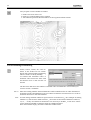
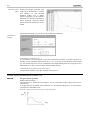
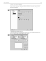
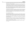
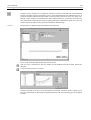
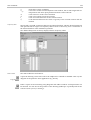
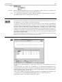
2.9.
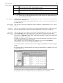
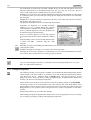
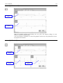
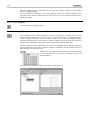
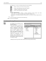
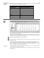
TABLE BROWSER ........................................................................................................................................................ 20
2.10.
REPORT MAKER ......................................................................................................................................................... 26
2.10.1. Report.................................................................................................................................................................... 27
2.10.2. Edit......................................................................................................................................................................... 28
2.10.3. Drawings .............................................................................................................................................................. 30
2.10.4. Gallery................................................................................................................................................................... 31
2.10.5. The Report Toolbar ............................................................................................................................................ 31
2.10.6. Gallery and Drawings Library Toolbars ........................................................................................................ 32
2.10.7. Text Editor............................................................................................................................................................ 32
2.11.
STORIES ...................................................................................................................................................................... 33
2.12.
LAYER MANAGER ...................................................................................................................................................... 33
2.13.
DRAWINGS LIBRARY .................................................................................................................................................. 33
2.14.
SAVE TO DRAWINGS LIBRARY................................................................................................................................... 33
2.15.
THE ICON BAR ............................................................................................................................................................ 34
2.15.1. Selection................................................................................................................................................................ 35
2.15.2. Zoom ..................................................................................................................................................................... 37
2.15.3. Views ..................................................................................................................................................................... 38
2.15.4. Workplanes .......................................................................................................................................................... 39
2.15.5. Geometric tranformations on objects ............................................................................................................. 40
2.15.5.1.
Translate ....................................................................................................................................................... 40
2.15.5.2.
Rotate ............................................................................................................................................................ 41
2.15.5.3.
Mirror............................................................................................................................................................ 42
2.15.5.4.
Scale............................................................................................................................................................... 42
2.15.6. Display Mode ...................................................................................................................................................... 43
2.15.7. Guidelines ............................................................................................................................................................ 45
2.15.8. Geometry Tools................................................................................................................................................... 46
2.15.9. Dimensions Lines, Symbols and Labels ......................................................................................................... 47
2.15.9.1.
Orthogonal Dimension Lines .................................................................................................................. 47
2.15.9.2.
Aligned Dimension Lines ......................................................................................................................... 50
2.15.9.3.
Angle Dimension........................................................................................................................................ 50
2.15.9.4.
Arc Length ................................................................................................................................................... 51
2.15.9.5.
Arc Radius.................................................................................................................................................... 51
2.15.9.6.
Level and Elevation Marks....................................................................................................................... 51
2.15.9.7.
Text Box ........................................................................................................................................................ 52
2.15.9.8.
Object Info and Result Text Boxes .......................................................................................................... 54
2.15.9.9.
Isoline labels ................................................................................................................................................ 56
2.15.10. Renaming/renumbering .................................................................................................................................... 56
2.15.11. Parts ....................................................................................................................................................................... 57
2.15.12. Sections ................................................................................................................................................................. 59
2.15.13. Find........................................................................................................................................................................ 61
2.15.14. Display Options .................................................................................................................................................. 62
4
2.15.15. Options ................................................................................................................................................................. 66
2.15.15.1. Grid and Cursor.......................................................................................................................................... 67
2.15.15.2. Editing........................................................................................................................................................... 68
2.15.15.3. Drawing........................................................................................................................................................ 69
2.15.16. Model Info ............................................................................................................................................................ 69
2.16.
SPEED BUTTONS......................................................................................................................................................... 70
2.17.
INFORMATION WINDOWS ........................................................................................................................................ 71
2.17.1. Info Window........................................................................................................................................................ 71
2.17.2. Coordinate Window........................................................................................................................................... 71
2.17.3. Color Legend Window ...................................................................................................................................... 71
2.17.4. Perspective Window Tool ................................................................................................................................. 73
3. THE MAIN MENU....................................................................................................................... 75
3.1.
FILE ............................................................................................................................................................................. 75
3.1.1.
New Model........................................................................................................................................................... 75
3.1.2.
Open...................................................................................................................................................................... 76
3.1.3.
Save........................................................................................................................................................................ 76
3.1.4.
Save As .................................................................................................................................................................. 76
3.1.5.
Export .................................................................................................................................................................... 77
3.1.6.
Import.................................................................................................................................................................... 78
3.1.7.
Tekla Structures – AxisVM connection........................................................................................................... 80
3.1.8.
Page Header......................................................................................................................................................... 83
3.1.9.
Print Setup............................................................................................................................................................ 83
3.1.10. Print ....................................................................................................................................................................... 84
3.1.11. Printing from File................................................................................................................................................ 86
3.1.12. Model Library ...................................................................................................................................................... 86
3.1.13. Material Library................................................................................................................................................... 87
3.1.14. Cross-Section Library ......................................................................................................................................... 90
3.1.14.1.
Cross-Section Editor................................................................................................................................... 94
3.1.15. Exit ......................................................................................................................................................................... 99
3.2.
EDIT .......................................................................................................................................................................... 100
3.2.1.
Undo .................................................................................................................................................................... 100
3.2.2.
Redo..................................................................................................................................................................... 100
3.2.3.
Select All.............................................................................................................................................................. 100
3.2.4.
Copy .................................................................................................................................................................... 100
3.2.5.
Paste..................................................................................................................................................................... 101
3.2.6.
Copy / paste options......................................................................................................................................... 101
3.2.7.
Delete................................................................................................................................................................... 102
3.2.8.
Table Browser .................................................................................................................................................... 103
3.2.9.
Report Maker ..................................................................................................................................................... 103
3.2.10. Saving drawings and design result tables ................................................................................................... 103
3.2.11. Weight Report ................................................................................................................................................... 103
3.2.12. Assemble structural members ........................................................................................................................ 103
3.2.13. Break apart structural members..................................................................................................................... 104
3.2.14. Convert surface loads distributed over beams ........................................................................................... 104
3.2.15. Convert automatic references ........................................................................................................................ 104
3.3.
SETTINGS .................................................................................................................................................................. 104
3.3.1.
Display ................................................................................................................................................................ 104
3.3.2.
Options ............................................................................................................................................................... 105
3.3.3.
Layer Manager .................................................................................................................................................. 105
3.3.4.
Stories .................................................................................................................................................................. 106
3.3.5.
Guidelines........................................................................................................................................................... 107
3.3.6.
Design Codes ..................................................................................................................................................... 108
3.3.7.
Units and Formats ............................................................................................................................................ 108
3.3.8.
Gravitation ......................................................................................................................................................... 108
3.3.9.
Preferences ......................................................................................................................................................... 109
3.3.10. Language ............................................................................................................................................................ 115
3.3.11. Report Language............................................................................................................................................... 115
3.3.12. Toolbars to default position ............................................................................................................................ 115
User’s Manual
3.4.
3.5.
3.5.1.
3.5.2.
3.5.3.
3.5.4.
3.5.5.
3.5.6.
3.5.7.
3.5.8.
3.6.
3.6.1.
3.6.2.
3.6.3.
3.6.4.
3.6.5.
3.7.
3.7.1.
3.7.2.
3.7.3.
3.7.4.
3.7.5.
3.7.6.
3.7.7.
3.7.8.
3.7.9.
3.7.10.
3.7.11.
3.7.12.
5
VIEW ......................................................................................................................................................................... 116
WINDOW .................................................................................................................................................................. 117
Property Editor.................................................................................................................................................. 117
Information Windows ..................................................................................................................................... 118
Background picture.......................................................................................................................................... 118
Split Horizontally.............................................................................................................................................. 119
Split Vertically ................................................................................................................................................... 119
Close Window ................................................................................................................................................... 120
Drawings Library.............................................................................................................................................. 120
Save to Drawings Library................................................................................................................................ 121
HELP ......................................................................................................................................................................... 122
Contents.............................................................................................................................................................. 122
AxisVM Home Page ......................................................................................................................................... 122
AxisVM Update................................................................................................................................................. 122
About ................................................................................................................................................................... 122
Release information.......................................................................................................................................... 122
MAIN TOOLBAR ....................................................................................................................................................... 123
New ..................................................................................................................................................................... 123
Open.................................................................................................................................................................... 123
Save...................................................................................................................................................................... 123
Print ..................................................................................................................................................................... 123
Undo.................................................................................................................................................................... 123
Redo..................................................................................................................................................................... 123
Layer Manager .................................................................................................................................................. 123
Stories .................................................................................................................................................................. 124
Table Browser .................................................................................................................................................... 124
Report Maker..................................................................................................................................................... 124
Drawings Library.............................................................................................................................................. 124
Save to Drawings Library................................................................................................................................ 124
4. THE PREPROCESSOR .............................................................................................................. 125
4.1.
4.2.
4.2.1.
4.3.
4.3.1.
4.3.2.
4.4.
4.5.
4.6.
4.7.
4.7.1.
4.7.2.
4.7.3.
4.7.4.
4.7.5.
4.7.6.
4.8.
4.8.1.
4.8.2.
4.8.3.
4.8.4.
4.8.5.
4.8.6.
4.8.7.
4.8.8.
4.8.9.
GEOMETRY ............................................................................................................................................................... 125
THE GEOMETRY EDITOR ......................................................................................................................................... 126
Multi-Window Mode ....................................................................................................................................... 126
COORDINATE SYSTEMS ........................................................................................................................................... 127
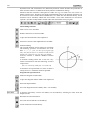
Cartesian Coordinate System......................................................................................................................... 127
Polar Coordinates ............................................................................................................................................. 127
COORDINATE WINDOW.......................................................................................................................................... 128
GRID ......................................................................................................................................................................... 128
CURSOR STEP ........................................................................................................................................................... 128
EDITING TOOLS ....................................................................................................................................................... 129
Cursor Identification ....................................................................................................................................... 129
Entering Coordinates Numerically ............................................................................................................... 130
Measuring Distance.......................................................................................................................................... 130
Constrained Cursor Movements ................................................................................................................... 130
Freezing Coordinates....................................................................................................................................... 132
Auto Intersect .................................................................................................................................................... 132
GEOMETRY TOOLBAR.............................................................................................................................................. 133
Node (Point) ...................................................................................................................................................... 133
Line ...................................................................................................................................................................... 133
Arc ........................................................................................................................................................................ 134
Horizontal Division .......................................................................................................................................... 135
Vertical Division................................................................................................................................................ 135
Quad/Triangle Division................................................................................................................................... 136
Line Division...................................................................................................................................................... 137
Intersect .............................................................................................................................................................. 138
Remove node..................................................................................................................................................... 138
6
4.8.10. Normal Transversal .......................................................................................................................................... 138
4.8.11. Intersect plane with the model ...................................................................................................................... 138
4.8.12. Intersect plane with the model and remove half space............................................................................ 138
4.8.13. Domain Intersection......................................................................................................................................... 138
4.8.14. Geometry Check ............................................................................................................................................... 139
4.8.15. Surface................................................................................................................................................................. 139
4.8.16. Modify, transform............................................................................................................................................. 140
4.8.17. Delete................................................................................................................................................................... 141
4.9.
FINITE ELEMENTS .................................................................................................................................................... 142
4.9.1.
Material ............................................................................................................................................................... 142
4.9.2.
Cross-Section ..................................................................................................................................................... 143
4.9.3.
Direct drawing of objects ................................................................................................................................ 144
4.9.4.
Domain................................................................................................................................................................ 145
4.9.4.1.
COBIAX-domain....................................................................................................................................... 146
4.9.5.
Hole...................................................................................................................................................................... 148
4.9.6.
Domain operations ........................................................................................................................................... 148
4.9.7.
Line Elements .................................................................................................................................................... 149
4.9.8.
Surface Elements............................................................................................................................................... 156
4.9.9.
Nodal Support ................................................................................................................................................... 159
4.9.10. Line Support ...................................................................................................................................................... 162
4.9.11. Surface Support................................................................................................................................................. 164
4.9.12. Edge hinge.......................................................................................................................................................... 164
4.9.13. Rigid elements ................................................................................................................................................... 165
4.9.14. Diaphragm ......................................................................................................................................................... 166
4.9.15. Spring .................................................................................................................................................................. 166
4.9.16. Gap....................................................................................................................................................................... 167
4.9.17. Link ...................................................................................................................................................................... 168
4.9.18. Nodal DOF (Degrees of Freedom) ................................................................................................................ 171
4.9.19. References .......................................................................................................................................................... 173
4.9.20. Creating model framework from an architectural model ........................................................................ 177
4.9.21. Modify ................................................................................................................................................................. 180
4.9.22. Delete................................................................................................................................................................... 180
4.10.
LOADS....................................................................................................................................................................... 181
4.10.1. Load Cases, Load Groups ............................................................................................................................... 181
4.10.2. Load Combination ............................................................................................................................................ 185
4.10.3. Nodal Loads....................................................................................................................................................... 186
4.10.4. Concentrated Load on Beam.......................................................................................................................... 187
4.10.5. Point Load on Domain..................................................................................................................................... 187
4.10.6. Distributed line load on beam/rib.................................................................................................................. 188
4.10.7. Edge Load........................................................................................................................................................... 189
4.10.8. Domain Line Load ............................................................................................................................................ 190
4.10.9. Surface Load ...................................................................................................................................................... 192
4.10.10. Domain Area Load............................................................................................................................................ 193
4.10.11. Surface load distributed over line elements ................................................................................................ 196
4.10.12. Fluid Load .......................................................................................................................................................... 197
4.10.13. Dead Load .......................................................................................................................................................... 197
4.10.14. Fault in Length (Fabrication Error) ............................................................................................................... 197
4.10.15. Tension/Compression ...................................................................................................................................... 198
4.10.16. Thermal Load on Line Elements ................................................................................................................... 198
4.10.17. Thermal Load on Surface Elements .............................................................................................................. 199
4.10.18. Forced Support Displacement........................................................................................................................ 199
4.10.19. Influence Line.................................................................................................................................................... 200
4.10.20. Seismic Loads..................................................................................................................................................... 200
4.10.20.1. Seismic calculation based on Eurocode 8 ............................................................................................ 203
4.10.20.2. Seismic calculation based on Swiss Code ............................................................................................ 207
4.10.20.3. Seismic calculation based on German Code ....................................................................................... 211
4.10.20.4. Seismic calculation based on Italian Code........................................................................................... 214
User’s Manual
7
4.10.21. Pushover loads .................................................................................................................................................. 218
4.10.22. Tensioning.......................................................................................................................................................... 221
4.10.23. Moving loads ..................................................................................................................................................... 227
4.10.23.1. Moving loads on line elements.............................................................................................................. 227
4.10.23.2. Moving loads on domains ...................................................................................................................... 228
4.10.24. Dynamic loads (for time-history analysis)................................................................................................... 229
4.10.25. Nodal Mass ........................................................................................................................................................ 233
4.10.26. Modify................................................................................................................................................................. 233
4.10.27. Delete .................................................................................................................................................................. 233
4.11.
MESH ........................................................................................................................................................................ 234
4.11.1. Mesh Generation .............................................................................................................................................. 234
4.11.1.1.
Meshing of line elements........................................................................................................................ 234
4.11.1.2.
Mesh generation on domain.................................................................................................................. 235
4.11.2. Mesh Refinement.............................................................................................................................................. 236
4.11.3. Checking finite elements................................................................................................................................. 237
5. ANALYSIS................................................................................................................................... 239
5.1.
5.2.
5.3.
5.4.
5.5.
5.6.
5.7.
STATIC ANALYSIS ..................................................................................................................................................... 241
VIBRATION ............................................................................................................................................................... 245
DYNAMIC ANALYSIS ................................................................................................................................................ 247
BUCKLING ................................................................................................................................................................ 249
FINITE ELEMENTS .................................................................................................................................................... 250
MAIN STEPS OF AN ANALYSIS ................................................................................................................................. 252
ERROR MESSAGES .................................................................................................................................................... 253
6. THE POSTPROCESSOR ........................................................................................................... 255
6.1.
STATIC ...................................................................................................................................................................... 255
6.1.1.
Minimum and Maximum Values .................................................................................................................. 259
6.1.2.
Animation........................................................................................................................................................... 260
6.1.3.
Diagram display ................................................................................................................................................ 261
6.1.4.
Pushover capacity curves................................................................................................................................ 263
6.1.4.1.
Capacity curves according to eurocode 8............................................................................................ 264
6.1.4.2.
Acceleration-Displacement Response Spectrum (ADRS) ................................................................ 264
6.1.5.
Result Tables ...................................................................................................................................................... 266
6.1.6.
Displacements ................................................................................................................................................... 267
6.1.7.
Truss/Beam Element Internal Forces ............................................................................................................ 268
6.1.8.
Rib Element Internal Forces ........................................................................................................................... 270
6.1.9.
Surface Elements Internal Forces .................................................................................................................. 270
6.1.10. Support Element Internal Forces................................................................................................................... 273
6.1.11. Internal forces of line to line link elements and edge hinges.................................................................. 274
6.1.12. Truss/Beam/Rib Element Stresses.................................................................................................................. 274
6.1.13. Surface Element Stresses ................................................................................................................................. 276
6.1.14. Influence Lines .................................................................................................................................................. 276
6.1.15. Unbalanced Loads ............................................................................................................................................ 277
6.2.
VIBRATION ............................................................................................................................................................... 278
6.3.
DYNAMIC ................................................................................................................................................................. 279
6.4.
BUCKLING ................................................................................................................................................................ 279
6.5.
R.C. DESIGN............................................................................................................................................................. 280
6.5.1.
Surface Reinforcement .................................................................................................................................... 280
6.5.1.1.
Calculation based on Eurocode 2.......................................................................................................... 281
6.5.1.2.
Calculating based on DIN 1045-1 and SIA 262 ................................................................................... 283
6.5.2.
Actual Reinforcement ...................................................................................................................................... 284
6.5.2.1.
Reinforcement for surface elements and domains............................................................................ 284
6.5.2.2.
Mesh-independent reinforcement........................................................................................................ 285
6.5.3.
Crack Opening Calculation ............................................................................................................................ 286
6.5.3.1.
Calculation based on Eurocode 2.......................................................................................................... 287
6.5.3.2.
Calculation based on DIN 1045-1.......................................................................................................... 287
8
6.5.4.
Non-linear deflection of RC plates................................................................................................................ 288
6.5.5.
Shear resistance calculation for plates and shells....................................................................................... 288
6.5.5.1.
Calculation based on Eurocode 2 .......................................................................................................... 289
6.5.6.
Column Reinforcement ................................................................................................................................... 289
6.5.6.1.
Check of reinforced columns based on Eurocode 2 .......................................................................... 295
6.5.6.2.
Check of reinforced columns based on DIN1045-1 ........................................................................... 296
6.5.6.3.
Check of reinforced columns based on SIA 262 ................................................................................. 297
6.5.7.
Beam reinforcement design............................................................................................................................ 298
6.5.7.1.
Beam Reinforcement Design based on Eurocode2............................................................................ 302
6.5.7.2.
Beam Reinforcement Design based on DIN 1045-1........................................................................... 304
6.5.7.3.
Beam Reinforcement Design based on SIA 262:2003 ........................................................................ 307
6.5.8.
Punching Analysis ............................................................................................................................................ 309
6.5.8.1.
Punching analysis based on Eurocode2............................................................................................... 311
6.5.8.2.
Punching analysis based on DIN 1045-1.............................................................................................. 313
6.5.9.
Footing design ................................................................................................................................................... 314
6.5.10. Design of COBIAX slabs .................................................................................................................................. 322
6.6.
STEEL DESIGN .......................................................................................................................................................... 324
6.6.1.
Steel beam design based on Eurocode 3 ...................................................................................................... 324
6.6.2.
Bolted Joint Design of Steel Beams ............................................................................................................... 332
6.7.
TIMBER BEAM DESIGN............................................................................................................................................. 336
7. AXISVM VIEWER AND VIEWER EXPERT.......................................................................... 345
8. PROGRAMMING AXISVM .................................................................................................... 347
9. STEP BY STEP INPUT SCHEMES .......................................................................................... 349
9.1.
9.2.
9.3.
9.4.
9.5.
PLANE TRUSS MODEL ............................................................................................................................................. 349
PLANE FRAME MODEL ............................................................................................................................................ 351
PLATE MODEL .......................................................................................................................................................... 353
MEMBRANE MODEL ................................................................................................................................................ 355
RESPONSE SPECTRUM ANALYSIS ............................................................................................................................ 357
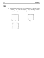
10. EXAMPLES .................................................................................................................................. 359
10.1.
10.2.
10.3.
10.4.
10.5.
10.6.
10.7.
10.8.
LINEAR STATIC ANALYSIS OF A STEEL PLANE FRAME........................................................................................... 359
GEOMETRIC NONLINEAR STATIC ANALYSIS OF A STEEL PLANE FRAME............................................................. 360
BUCKLING ANALYSIS OF A STEEL PLANE FRAME .................................................................................................. 361
VIBRATION ANALYSIS (I-ORDER) OF A STEEL PLANE FRAME .............................................................................. 362
VIBRATION ANALYSIS (II-ORDER) OF A STEEL PLANE FRAME ............................................................................. 363
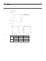
LINEAR STATIC ANALYSIS OF A REINFORCED CONCRETE CANTILEVER ............................................................. 364
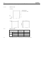
LINEAR STATIC ANALYSIS OF A SIMPLY SUPPORTED REINFORCED CONCRETE PLATE...................................... 365
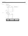
LINEAR STATIC ANALYSIS OF A CLAMPED REINFORCED CONCRETE PLATE ...................................................... 366
11. REFERENCES.............................................................................................................................. 367
User’s Manual
1.
9
New features in Version 10
General
New display style to help users with high resolution monitors
Architectural rendering
Exporting SDNF file
Export of parts or selected elements to AXS file
2.15.6 Display Mode
3.1.5 Export
New DXF import options (import of visible layers, creating parts using layer
information)
3.1.6 Import
Automatically updated logical parts
2.15.11 Parts
Renaming / renumbering elements
Definition of stories
2.15.10
Renaming/renumbering
3.3.4 Stories
IFC enhancements (improved processing of BREP andIFCBuildingElementProxy)
3.1.6 Import
Editing
Removal of intersections
4.8.9 Remove node
Editing on stories
3.3.4 Stories
Detachment of objects
4.8.16 Modify, transform
Cutting multiple domains
4.8.11 Intersect plane with
the model
4.8.12 Intersect plane with
the model and remove
half space
4.8.16 Modify, transform
Cutting objects with a plane
New editing functions on pet palettes (detach, cutoff, tangential arc)
New constraints (point of intersection for two lines, dividing point betweeen to
nodes)
2.15.8 Geometry Tools
Structural copy & paste functions (customizable through Edit / Copy/paste options)
3.2.6 Copy / paste options
New functions in the COM server
Elements
Timber database with material parameters according to Eurocode5
6.7 Timber Beam Design
Rib definition with automatic eccentricity update
4.9.7 Line Elements
Nonlinear link elements (tension only / compression only)
4.9.17 Link
10
Loads
Polygonal or arced line loads
4.10.6 Distributed line load
on beam/rib
4.10.8 Domain Line Load
Polygonal, arced or complex polygonal surface loads
4.10.10 Domain Area Load
Edge loads can be defined on internal lines of a domain
4.10.7 Edge Load
Smart labeling of line loads
Optimization of surface loads distributed over beams and ribs for multiple core
processors
Analysis
Pushover Analysis according to EC8
Analysis information can be reviewed any time using the Model information dialog
4.10.21 Pushover loads
6.1.4 Pushover capacity
curves
2.15.16 Model Info
New analisys engine optimized for multiple cores / threads can reach more memory
than before
5 Analysis
Dynamic analysis (module DYN)
5.3 Dynamic Analysis
Increment function editor for nonlinear analysis
5.1 Static Analysis
Results
Design of COBIAX slabs
Display of average support forces on line supports
Display of elastic hinges at beam ends
New result tables (beam, rib, truss forces for different load cases)
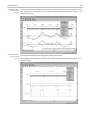
Improved diagram display
6.5.10 Design of COBIAX
slabs
6.1.10 Support Element
Internal Forces
4.9.7 Line Elements
6.1.7 Truss/Beam Element
Internal Forces
6.1.8 Rib Element Internal
Forces
6.1.3 Diagram display
Design
Cross-sections of Class 4 can be designed
Pad footing design according to Eurocode 7 calculating footing size and
reinforcement (module RC4)
Timber design according to Eurocode 5 (module TD1)
6.6.1 Steel beam design
based on Eurocode 3
6.5.9 Footing design
6.7 Timber Beam Design
User’s Manual
2.
11
How to Use AxisVM
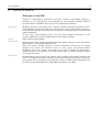
Welcome to AxisVM!
AxisVM is a finite-element program for the static, vibration, and buckling analysis of
structures. It was developed by and especially for civil engineers. AxisVM combines
powerful analysis capabilities with an easy to use graphical user interface.
Preprocessing
Modeling: geometry tools (point, lines, surfaces); automatic meshing; material and crosssection libraries; element and load tools, import/export CAD geometry (DXF); interface to
architectural design software products like Graphisoft’s ArchiCAD via IFC to create model
framework directly.
At every step of the modeling process, you will receive graphical verification of your
progress. Multi-level undo/redo command and on-line help is available.
Analysis
Static, vibration, and buckling
Postprocessing
Displaying the results: deformed/undeformed shape display; diagram, and iso-line/surface
plots; animation; customizable tabular reports.
After your analysis, AxisVM provides powerful visualization tools that let you quickly
interpret your results, and numerical tools to search, report, and perform further
calculations using those results. The results can be used to display the deformed or
animated shape of your geometry or the isoline/surface plots. AxisVM can linearly combine
or envelope the results.
Documentation
Documentation is always part of the analysis, and a graphical user interface enhances the
process and simplifies the effort. AxisVM provides direct, high quality printing of both text
and graphics data to document your model and results. In addition data and graphics can
be easily exported (DXF, BMP, JPG, WMF, EMF, RTF, HTML, TXT, DBF).
12
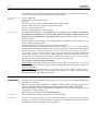
2.1. Hardware Requirements
The table below shows the minimum/recommended hardware and software requirements,
so you can experience maximum productivity with AxisVM.
Recommended configuration
at least 1 GB RAM
at least 2 GB of free hard disk space
CD drive
XGA color monitor (at least 1024x768, 1280x1024 recommended)
Windows 2000 / XP/ Vista / Windows 7 operating system
Mouse or other pointing device
Windows compatible laser or inkjet printer
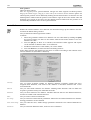
Memory access
To reach more memory is very important as it speeds up the analysis considerably.
To enable advanced memory access is possible under Professional or Ultimate editions of
Windows Vista and Windows 7 operating systems. Home Premium edition does not support this feature
If the computer has more than 4 GB of physical RAM, AxisVM10 can access memory over
4 GB on 32-bit operating systems.
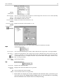
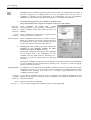
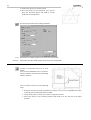
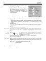
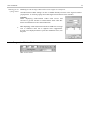
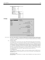
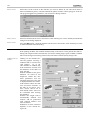
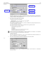
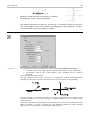
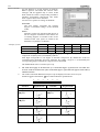
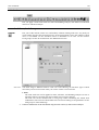
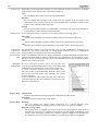
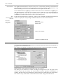
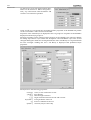
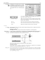
To turn this function ot it is necessary to lock pages in memory:
After invoking the Run command from the Start menu type gpedit.msc. After clicking
the OK button a Windows application named Group Policy opens. Find the following item in
the tree on the left: Computer Configuration / Windows Settings / Security Settings / Local Policies
/ User Rights Assignment. Then find Lock pages in memory in the list on the right. Double click
on this item. In the Local Policy Sertings dialog click the Add button then add the users or
user groups who needs access to the memory above 4 GB. Close Local Policy Settings dialog
then close Group Policy by clicking the Close icon in the top right corner.
User Account Control must also be disabled.
Under Vista: Launch MSCONFIG from the Run menu. Find and click Disable UAC on the
Tools tab. Close the command window when the command is done. Close MSCONFIG and
restart the computer.
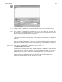
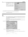
Under Windows 7: Find Start Menu / Control Panel / User Accounts. Click on Change User Account Control settings link. Set the slider tothe lowest value (Never Notify). Click OK to make
the change effective and restart the computer.
2.2. Installation
Software Protection
The program is protected by a hardware key. Two types of key are available: parallel port
(LPT) keys and USB keys.
Plug the key only after installation is complete, because certain operating systems try to
recognize the plugged device and this process may interfere with the driver installation.
Non-network drivers will be automatically installed. If you encountered problems you can
install this driver later from the CD.
Run the Startup program and select Reinstall driver .
Standard Key
First install the program then plug the key into the computer.
Network Keys
If you have a network version you must install the network key. In most cases AxisVM and
the key are on different computers but to make the key available through the network the
Sentinel driver must be installed on both computers.
User’s Manual
13
AxisVM Version 10 is shipped with a parallel port or USB Sentinel Super Pro dongle but
earlier customers may have parallel port NetSentinel dongle.
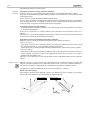
a. Sentinel SuperPro dongle
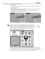
1. Insert the AxisVM CD in the CD-ROM drive of the AxisVM server.
Run [CD Drive]: \ Startup.exe. Select Reinstall driver. This type of network key
requires at least a 7.1 driver. CD contains the 7.5 version of the driver.
2. Connect the key to the parallel or USB port of one of the computers. This way you
select the AxisVM server.
To run AxisVM on any computer on the network SuperPro Server must be running on the
server. If it stops all running AxisVM programs stop.
b. NetSentinel dongle
1. Insert the AxisVM CD in the CD-ROM drive of the AxisVM server.
Run [CD Drive]: \ Sentinel \ English \ Driver\ setup.exe to install Sentinel driver.
2. Connect the key to the parallel port of one of the computers. This way you select the
AxisVM server.
3. Copy the contents of the folder [CD Drive]: \ Sentinel \ English \ server \ Disk1 \
Win32 to a folder of the server’s hard drive.
4. Run NSRVGX.EXE from that folder. This server program handles the network key
and communicates with the applications on the network.
To run AxisVM on any computer on the network NSRVGX must be running on the server.
If NSRVGX stops all running AxisVM programs stop.
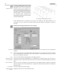
Installation
AxisVM runs on 2000 / XP / Vista / Windows 7 operating systems.
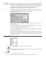
Insert the AxisVM CD into the CD drive. The Startup program starts automatically if the
autoplay option is enabled. If Autoplay is not enabled, click the Start button, and select
Run... . Open the Startup.exe program on your AxisVM CD. Select AxisVM 10 Setup and
follow the instructions.
If the setup program cannot be launched or the following message appears: AUTOEXEC.NT The system file is not suitable for running MS-DOS and Microsoft Windows applications,
a Windows system file must be missing.
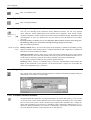
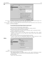
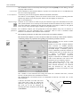
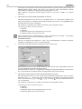
Installation under Vista Operating System:
• You need the latest Sentinel driver. You can download it: www.axisvm.eu / Support- Service Pack for AxisVM 10
• Click on the program icon with the Mouse right button after the installation of
AxisVM program
• Choose the Properties menu item from the Quick Menu.
•
Select the Compatibility tab on the appearing dialog and turn on the Run as administrator checkbox.
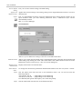
By default the program and the example models will be installed on drive C: in
C:\Program Files\AxisVM10
and
C:\Program Files\AxisVM10\Examples
folders. You can specify the drive and the folders during the installation process. The setup
program creates the AxisVM program group that includes the AxisVM application icon.
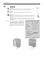
14
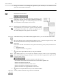
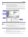
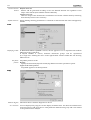
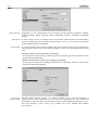
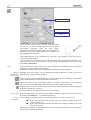
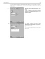
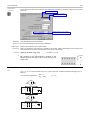
Starting AxisVM
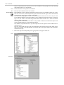
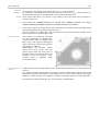
Click the Start button, select Programs, AxisVM folder, and click the AxisVM10 icon.
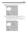
At startup a splash screen is displayed (see... 3.6.4 About) then a welcome screen is shown
where you can select a previous model or start a new one.
Clearing the checkbox at the bottom turns the welcome screen off for the future. To turn it
on choose the Settings\Preferences\Data Integrity dialog and check the Show welcome screen on
strartup checkbox.
Upgrading
It is recommended to install the new version to a new folder. This way the previous version
will remain available.
Converting earlier
models
Models created in a previous versions are recognized and converted automatically. Saving
files will use the latest format by default. Saving files in the file format of one of the previous
versions (6, 7, 8, 9) is possible but this way the information specific to the newer versions
will be lost.
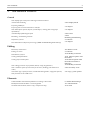
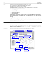
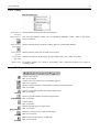
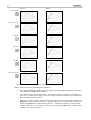
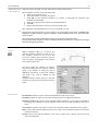
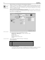
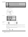
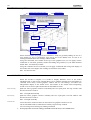
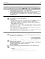
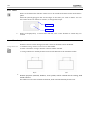
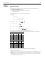
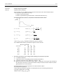
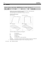
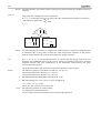
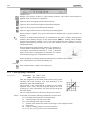
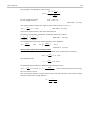
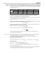
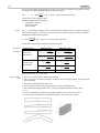
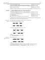
Steps of an analysis
The main steps of an analysis using AxisVM are:
Creating the Model (Preprocessing)
Static
(linear/nonlinear)
Analysis
Vibration
Dynamic
(first/second-order)
(linear/nonlinear)
Buckling
Evaluating the Results (Postprocessing)
Capacity
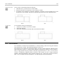
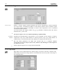
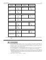
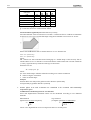
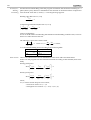
Practically, the model size is limited by the amount of free space on your hard disk.
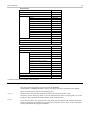
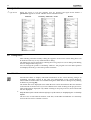
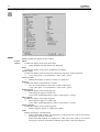
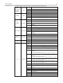
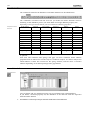
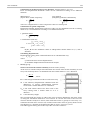
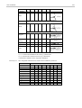
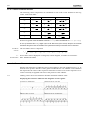
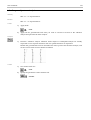
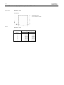
The restrictions on the model size and on the parameters of an analysis are as follows:
User’s Manual
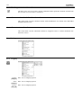
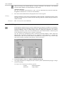
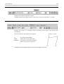
15
Professional
Entity
Nodes
Materials
Elements
Truss
Beam
Rib
Membrane
Plate
Shell
Support
Gap
Diaphragm
Spring
Rigid
Link
Load cases
Load combinations
Frequencies
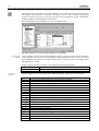
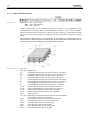
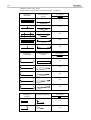
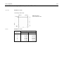
Small Business
Entity
Nodes
Materials
Elements
Only trusses
Truss+Beam+Rib *
Rib on the edge of a surface
Any combination of
membrane, plate or shell
Support
Gap
Diaphragm
Spring
Rigid
Link
Load cases
Load combinations
Frequencies (modal shapes)
Maximum
Unlimited
Unlimited
Unlimited
Unlimited
Unlimited
Unlimited
Unlimited
Unlimited
Unlimited
Unlimited
Unlimited
Unlimited
Unlimited
Unlimited
Unlimited
Unlimited
Unlimited
Maximum
Unlimited
Unlimited
500
250
1000
1500
Unlimited
Unlimited
Unlimited
Unlimited
Unlimited
Unlimited
99
Unlimited
30
* If there are beams or/and ribs in the structure
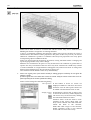
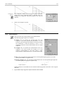
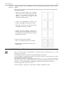
2.3. Getting Started
Step-by-step input schemes are presented in the Section 9.
See Example 1 of Chapter 10 with a step-by-step input scheme in 9.2 Plane Frame Model
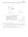
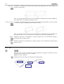
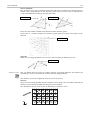
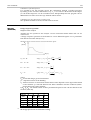
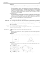
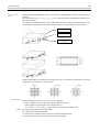
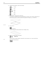
There are three major steps in a modeling process:
Geometry
The first step is to create the geometry model of the structure (in 2D or 3D).
Geometry can be drawn by hand or can be imported from other CAD programs. It is also
possible to draw elements (columns, beams, walls, slabs) directly.
Elements
If you chose to draw the geometry first you must specify material and element properties,
mesh the geometry into elements (assigning the properties and a mesh, to the wire-frame
model), and define the support conditions.
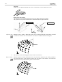
16
Loads
In the third step you must apply different loads on the model.
The end result will be a finite element model of the structure.
Once the model is created it is ready for analysis.
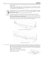
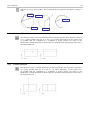
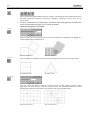
In Chapter 7, the step-by-step modeling of a few typical structures are presented.
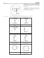
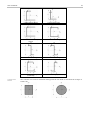
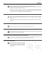
The following types of structures are shown:
1. Plane truss girder
2. Plane frame
3. Plate structure
4. Membrane cantilever
5. Seismic analysis
Understanding of these simple models will allow you to easily build more complex models.
It is recommended that you read the entire User’s Manual at least once while exploring
AxisVM.
In Chapter 1 you can find the timely, new features of the version.
Chapter 2 contains general information about using AxisVM. In other chapters the
explanation follows the pre- and postprocessor menu structures. Please consult this User’s
Manual every time you are using AxisVM.
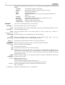
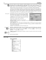
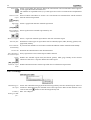
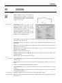
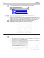
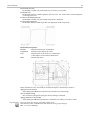
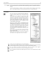
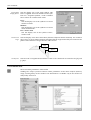
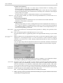
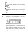
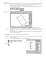
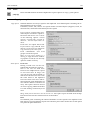
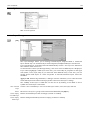
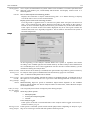
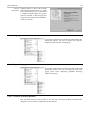
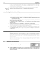
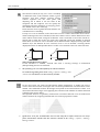
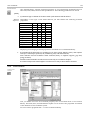
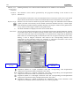
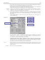
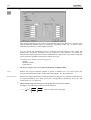
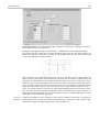
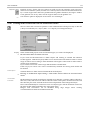
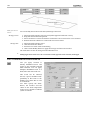
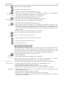
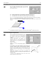
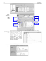
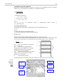
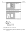
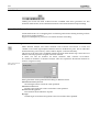
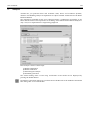
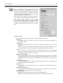
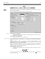
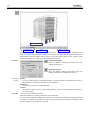
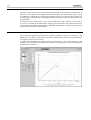
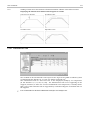
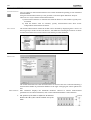
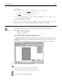
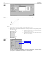
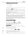
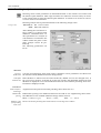
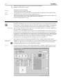
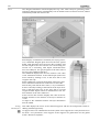
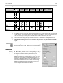
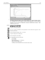
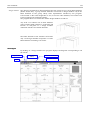
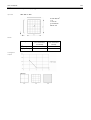
2.4. AxisVM User Interface
This section describes the working environment of the full AxisVM graphical user interface.
Please read these instructions carefully. Your knowledge of the program increases the
modeling speed and productivity.
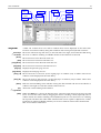
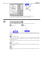
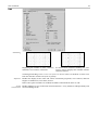
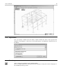
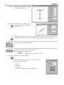
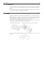
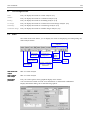
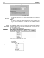
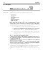
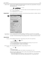
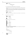
AxisVM screen
After you start AxisVM a screen similar to the following picture appears:
Model name and location path
Top menu bar
Pop-up
rowicon
Perspective Toolbar
Status window Color legend window
cursor
Moveable Icon bar
Property
Editor
Graphics
area
Pet palette
Coordinate
window
Context sensitive
help message
Speed buttons
User’s Manual
17
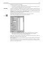
The parts of the AxisVM screen are briefly described below.
Graphics area
The area on the screen where you create your model.
Graphics cursor
The screen cursor is used to draw, select entities, and pick from menus and dialog boxes.
Depending on the current state of AxisVM, it can appear as a pick-box, crosshairs with pickbox, or pointer.
Top menu bar
Each item of the top menu bar has its own dropdown menu list. To use the top menu bar,
move the cursor up to the menu bar. The cursor will change to a pointer. To select a menu
bar item, move the pointer over it, and press the pick button to select the item. Its associated
sub-menu will appear.
Active icon
Icon bar
The active icon represents the command that is currently selected.
The icons represent working tools in a pictorial form. These tools are accessible during any
stage of work. The icon bar and flyout toolbars are draggable and dockable.
The window on the graphics area displaying the graphics cursor coordinates.
Coordinate
window
Color legend
window
Info window
Context sensitive
help
Property Editor
Pet palette
Speed buttons
The model
The window shows the color legend used in the display of the results. Appears only in the
post-processing session.
The window shows the status of the model and results display.
Provides a help message that depends on the topic under process.
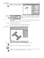
The Property Editor offers a simple way to change certain properties of the selected
elements or loads.
Pet palettes appear when modifying geometry according to the type of the dragged entity
(node, straight line, arc). See... 4.8.16 Modify, transform
Speed buttons in the bottom right provide the fastest access to certain switches (parts,
sections, symbols, numbering, workplanes, etc.)
With AxisVM you can create and analyze finite element models of civil engineering
structures. Thus the program operates on a model that is an approximate of the actual
structure.
To each model you must assign a name. That name will be used as a file name when it is
saved. You may assign only names that are valid Windows file names. The model consists
of all data that you specify using AxisVM. The model’s data are stored in two files: the input
data in the filename.axs and the results in the filename.axe file.
AxisVM checks if AXS and AXE files belong to the same version of the model.
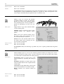
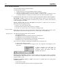
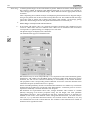
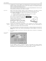
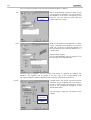
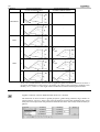
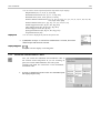
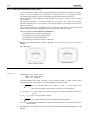
2.5. Using the Cursor, the Keyboard, the Mouse
Graphics
Graphics cursor
As you move your mouse, the graphics cursor symbol tracks the movement on the screen.
To select an entity, an icon or menu item, move the cursor over it and click the left mouse
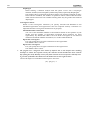
button. The shape of the cursor will change accordingly (see... 4.7.1 Cursor Identification),
and will appear on the screen in one of the following forms:
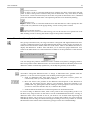
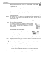
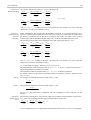
Crosshairs:
Pointer:
Crosshairs/zoom mode:
If you pick an entity when the cursor is in its default mode (info mode), the properties of
that entity will be displayed as a tool tip.
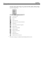
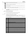
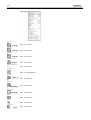
18
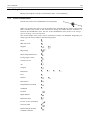
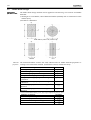
Depending on the menu your cursor is on, you may get the properties of the following
entities:
Geometry
Elements
Loads
Mesh
Static
Vibration
Dynamic
R.C. Design
Steel Design
Timber Design
The keyboard
node (point) coordinates, line length
finite element, reference, degree-of-freedom, support
element load, nodal mass
meshing parameters
displacement, internal force, stress, reinforcement, influence line
ordinate
mode shape ordinate
displacement, velocity, acceleration, internal force, stress
specific reinforcement values
efficiency results and resistances
utilization factor results and resistances
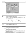
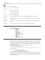
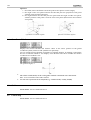
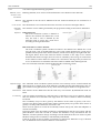
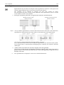
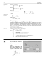
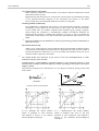
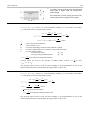
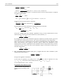
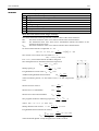
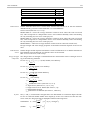
You can also use the keyboard to move the cursor:
Arrow keys, Moves the graphics cursor in the current plane.
[Ctrl] +
Arrow keys, Moves the graphics cursor in the current plane with a step size enlarged/reduced by a factor
set in the Settings dialog box.
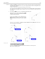
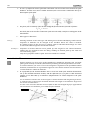
[Shift]+
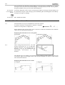
Moves the graphics cursor in the current plane on a line of angle n·∆α , custom α or
α +n·90°.
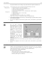
[↑][↓][←][→],
[Home] [End]
Moves the graphics cursor perpendicular to the current plane.
[Ctrl]+
[Home], [End]
Moves the graphics cursor perpendicular to the current plane with a step size
enlarged/reduced by a factor set in the Settings dialog box.
[Esc] or right button
[Enter]+[Space]
left button
[Alt]
[Tab]
Interrupts the command and/or returns to an upper menu level.
Selects an item from a menu, executes a command, and selects entities.
These are termed command buttons.
Activates the main menu
Moves the focus from control to control in a dialog.
[+] [-]
Performs fast zoom in/out and pan. The zoom and pan parameters are defined by the
current position of the graphics cursor in the graphics area, and by the magnification factor
set in Settings / Options / Zoom Factor. Center of the fast zoom in/out is always the current
graphics cursor position.
[Insert]
or [Alt]+[Shift]
Moves the relative origin (i.e. the reference point of the relative coordinates) to the current
graphics cursor position.
wheel Roll forward to zoom in
Roll backwards to zoom out
Press the wheel and drag to drag the drawing area
Centre of zoom in and zoom out is the current position of the cursor.
Hot Keys
Keyboard combinations to access frequently used functions faster.
See... 2.6 Hot Keys
right button Displays the Quick Menu. See... 2.7 Quick Menu
User’s Manual
19
2.6. Hot Keys
General Hot Keys
[Ctrl]+ [ [ ]
Zoom to fit
X-Z view
X-Y view
Y-Z view
Perspective view
Print
Select All (adds all entities to the
selection list)
View undo
[Ctrl]+ [ ] ]
[Ctrl]+[W]
[Ctrl]+ [1]
[Ctrl]+ [2]
[Ctrl]+ [3]
[Ctrl]+ [4]
[Ctrl]+ [P]
[Ctrl]+ [A]
[Ctrl]+[Z]
[Shift]+[Ctrl]+ [Z]
[Tab]
[Ctrl]+[R]
[Ctrl]+ [Q]
[Ctrl]+ [C]
[Ctrl]+[V]
[Alt]
[+]
[-]
[Ctrl]+ [O]
[Ctrl]+ [S]
[Del]
[Ctrl]+ [D]
[Ctrl]+[L]
Labels
View redo
[Ctrl]+[Y]
Symbols
Undo
Redo
Move between graphics windows
Refresh drawing (redraw)
Exit
Copy (to clipboard)
Paste (from clipboard)
[Ctrl]+[E]
Reverse local x direction of line elements
[F1]
[F7]
[F8]
[F9]
[F10]
[F11]
[F12]
Hot Keys in Tables
[Ctrl]+[L]
[Alt]+[F4]
[Ctrl]+[Insert]
[Ctrl]+[Del]
[Ctrl]+[A]
[F5]
[Ctrl]+[D]
[Ctrl]+ [Alt]+[F]
[Ctrl]+[R]
[Ctrl]+[G]
[Ctrl]+[M]
[F1]
[F9]
[F10]
Browse Libraries
Exit
New line
Delete line
Select all
Jump to line
Default format
Set column format
Set result display mode (for result tables)
Edit new cross-section (for cross-section tables)
Modify cross-section (for cross-section tables)
Context sensitive help
Add table to the report
Report Maker
Hot keys in the Report Maker
[Ctrl]+[T]
[Ctrl]+ [Alt]+[B]
[Ctrl]+[W]
[F3]
[Ctrl]+[P]
[Ctrl]+[Del]
Go to main menu
Zoom in
Zoom out
Open
Save
Delete entities/properties
Switches
Insert text
Insert Page Break
Export to RTF file
Report Preview
Print
Delete
Context-sensitive help
Set stories
Weight Report
Save drawing to the Drawings Library
Report Maker
Layer Manager
Table Browser
20
2.7. Quick Menu
right button
When the cursor is over the graphics area, by pressing the right mouse button a
quick menu appears in accord with the current command in use.
Selection
Geometry / Elements / Loads
Results
2.8. Dialog Boxes
After selecting a function usually a dialog box appears on the screen. These dialog boxes can
be used the same way as any other Windows dialog.
The dialog font can be changed by selecting the Settings\Preferences\Fonts dialog and clicking
the font sample label Dialog boxes.
You can change the position of all dialog windows. The program saves the latest position
and displays the dialog on the same position next time.
2.9. Table Browser
[F12]
AxisVM uses tables to display numerical information on the screen allowing changes in
formatting. The tables operate in the same way independent of the content displayed.
All the tables AxisVM creates are available through the Table Browser dialog box by clicking
its button or pressing [F12].
The model data to be displayed in the Table Browser can be selected from the tree structure
in the left side of the browser. If you use Table Browser while working in the pre-processor,
input model data is displayed only. While working in the post-processor, the model results
are also displayed.
Only the data of the current selection (if any) or of the active (i.e. displayed) part is listed by
default.
The tree view on the left lists element / load data, result tables and libraries in a hierarchy
and can also be used as a model overview.
User’s Manual
21
Add New
Row
Cross-Section
Editor
Copy
Paste
Format
Delete
Library
Using the table
Print
Fit
Add to
Report
A table can contain more rows and/or columns than can be displayed at the same time.
It can be viewed in its entirety using the scroll bars and/or using the keyboard as follows:
Arrow keys
left button
Moves the edit focus up and down, to the left and to the right, and scrolls the table along
the rows or columns. Clicking an editable cell moves the edit focus to that cell.
[Home]
Moves the focus to the first cell of the row.
[End]
Moves the focus to the last cell of the row.
[Ctrl]+[Home]
Moves the focus to the first cell of the first row
[Ctrl]+[End]
Moves the focus to the last cell of the last row.
[Page Up]
[Page Down]
Displays the previous page of rows.
Displays the next page of rows.
[Ctrl]+ [→
→]
Moves the focus to the next (to the right) page of columns (only in tables where more
columns can be displayed at the same time).
[Ctrl]+ [←
←]
Moves the focus to the previous (to the left) page of columns (only in tables where more
columns can be displayed at the same time).
[Enter]
Ends the current editing in the edit box storing the data entered and moves the edit box a
column to the right or to the first column of the next row.
[Esc]
right button
[Shift]
Aborts the current editing in the edit box.
While the [Shift] key is down all direction keys will select cells instead of moving the edit
focus. You can also select cells by dragging the mouse. Clicking a fixed (topmost) cell of a
column selects the column. Clicking a fixed (leftmost) cell of a row selects the row. Clicking
the top left cell selects the entire table. Selected cells can be copied to clipboard as a table.
If selection is within an editable column you can set a common value for the selected cells.
See... Set Common Value below
22
File
Browse Library
, [Ctrl]+ [L]
Loads cross-sectional or material data from a library. You can also save the current content
of the table in a custom library.
Import DBase File
Imports a DBase file name.dbf into the current table. The program checks the values of the
fields and sends an error message if an incompatible value is found.
Save As DBase
File
Exports the current table into a Dbase file name.dbf. The field names are generated based on
the names of the columns. The fields will be of text type.
Save As HTML
Exports the current table into an HTML file name.htm. This file can be imported as a table
into Word or can be opened in web browser applications. Some formatting information of
the columns will be lost.
Save As TXT
Exports the current table into a TXT (ASCII) file name.txt.
Save As RTF
Exports the current table into an RTF file name.rtf using the current template file. You can
import this file into Microsoft Word or any other word processor which can import RTF
files. See... 2.10.1 Report
New CrossSection Table
Creates a new cross-section data file name.sec. The table created will be placed together with
the cross-sections of the same type.
You can store cross sections of any type in these tables. Type of the table determines only
the position of the table in the Cross-section Library.
CrossSectionTable
Properties
You can modify properties (table’s name, cross.section type) of a user defined table.
Delete Cross
Sectin Table
You can delete a user defined table.
Print
, [Ctrl]+ [P]
Exit
[Alt]+ [F4]
Prints all the information displayed in the table to the selected printer or to a file, with the
page header and comment row previously set with the File/Header menu command.
Exits the table in the same way as the Cancel button (the changes are not saved).
User’s Manual
23
Edit
New Row
[Ctrl]+
[Insert]
Delete Rows
Adds a new row to the list, and allows you to fill all the editable cells with data in a fixed
order from left to right.
Deletes the selected rows. Also available in the popup menu.
[Ctrl]+ [Del]
Delete textures
Select Table
[Ctrl]+ [A]
Design New
Custom Crosssection
Available only if materials are listed. Removes texture from the
selected materials. Available in the popup menu.
Selects the entire table. Clicking the top left cell does the same.
Starts the graphics Cross-Section Editor, allowing the input of a new custom cross-section.
[Ctrl]+[G]
Modify Custom
Cross-section
Starts the graphics Cross-Section Editor, allowing the modification of a custom cross-section
previously created with the graphics Cross-Section Editor.
[Ctrl]+[M]
Automatic crosssection shape
update
Delete unused
cross-sections
Copy
If this function is on changing section parameters in the table leads to the recalculation of
geometry and cross-section parameters.
Unused cross-sections will be deleted from the table.
Copies selected cells to the Clipboard as a table. Also available in the popup menu.
[Ctrl]+ [C]
Paste
[Ctrl]+ [V]
Set Common
Value
Go to
[F5]
Pastes table cells from the Clipboard overwriting cell values.
If any of the values is unacceptable Paste aborts.
If entire rows were cut or copied and the table allows inserting new rows you can also add
clipboard data to the end of the table instead of overwriting the existing rows.
Sets a common value for the selected cells within a column.
Example: you can set the Z coordinate of all nodes to the same value making the model
absolutely flat. Available from the Table Browser Menu / Edit / Set Common Value.
Also available in the popup menu.
Jumps to a specified row in the table.
24
Format
During model
building
Turn on/off
columns
[Ctrl]+ [Alt]+ [F]
You can specify whether a column is visible or not, by setting the check boxes of the
corresponding columns.
The display format is set according to the settings in the Units/Settings dialogue window
(See... 3.3.7 Units and Formats).
Many cells require the entry of a numeric value. When entering real numbers you can use
the following characters:
+-01234567890E
and the standard Windows decimal separator specified in Start / Settings / Control Panel /
Regional Settings / Number / Decimal symbol field.
In some cases you cannot enter a negative number so the - key is deactivated while entering
these kind of values. If an integer value is required you cannot use the decimal separator
and E.
Format Defaults
[Ctrl]+ [D]
Restores the default format of the entire table (column visibility and decimals).
Order of load
cases...
The display order of load cases can be customized.
See... 4.10.1 Load Cases, Load Groups
Intermadiate
sections
After dividing or meshing beams or ribs with variable cross-section AxisVM builds up intermediate cross-sections. This menu item is to turn on/off the display of intermediate crosssections at the end of the list.
Show used crosssections in
boldface
After the Delete unused cross-sections
command only the sections in bold
will remain in the list.
The cross-names which are signed by bold letter will remain in the table if the Delete Unused
Cross-sections switch is turned on.
In case of result query new items appear on the Format menu and the Toolbar.
User’s Manual
25
During
result query
Result Display
Options
[Ctrl]+[R]
Results On/Off
You can control finding the extremes for result components and set to show results (Result)
and/or just the extremes (Extremes).
See in detail: 6.1.5 Result Tables
Display of results can be turned on / off.
[Ctrl]+[T]
Extremes On/Off
Display of extremes can be turned on / off.
[Ctrl]+[E]
Property Filtering
[CTRL]+[Q]
Property filtering helps you to select which elements to include in the table.
Report
Current report
Add table to
report
[F9]
Report Maker
[F10]
You can set the current report. Tables will be added to this report. See... 2.10 Report Maker
Adds the current table to the current report. If the selected node in the treeview has subnodes (e.g. MODEL or Loads) all tables under that node will be added. If the current table is
a result table and is set to display extremes only all sub-tables will display extremes only.
See... 2.10 Report Maker.
Opens Report Maker.
Help
About Table
Displays info about the table.
About Table
Browser
Displays info about the table browser operation.
OK
Cancel
Saves the data and closes the table.
Closes the table without saving the data.
Result tables also display the extremes (minimum and maximum values) of the data if you
select this option in the Display Options dialog when you enter Table Browser. Displaying
both the individual values and the extremes is the default setting.
26
2.10. Report Maker
[F10]
Report Maker is a tool to compile a full report of a project using report items
(tables/drawings/pictures created by AxisVM and user-defined text blocks). Reports are
stored in the model file (*.axs) and can be printed or saved as a Rich Text Format (RTF) file.
RTF files can be processed by other programs (e.g. Microsoft Word).
Tables ex ported from Table Browser are automatically updated if the model has been
changed or some of its parts were deleted.
Report Maker can handle several different reports for the same project. The structure of
reports is displayed in a tree view on the left. The properties of the selected report item are
shown on the right side of the window.
Table
If a table is selected, its comment text, column titles and other properties are shown. Display
of title, comment and columns can be turned on and off.
Text
If a text block is selected the text is shown on the right. Click the button
Edit text... to make changes.
Picture or Drawing
If a picture or drawing is selected it is shown on the right. Its size, alignment and caption
can be set.
User’s Manual
27
Drawings Library
By clicking the Drawings Library tab you can browse the saved drawings and add the
selected ones to the report. Unlike the pictures in the Gallery these drawings are not
graphics files, but view settings stored to recreate the drawing at any time. This way
drawings will be automatically updated if we change and recalculate the model.
See in detail... 3.5.7 Drawings Library, 3.5.8 Save to Drawings Library.
Gallery
By clicking the Gallery tab you can browse the saved pictures (BMP, JPG, WMF, EMF)
located in a folder named Images_modelname and add the selected ones to the report. This
folder is automatically created as a subfolder of the model folder.
See in detail... 2.10.4 Gallery
Click the Settings... button to change the caption, size, justification, rotation color mode or
scaling of drawings.
You can save the current drawing on screen or the result tables in design modules with the
function of Edit\ Saving drawings and design result tables in main menu.
See... 3.2.10 Saving drawings and design result tables
One or more selected pictures in the Gallery can be inserted into a report
by selecting menu item Gallery/Add pictures to the report or clicking the arrow button above
the Gallery or by drag and drop.
In printed reports Report Maker automatically builds a table of contents and inserts it to the
beginning of the report. Tables are listed according to their titles. Text blocks are listed only
if they were formatted using one of the Heading styles in the Text Editor. Pictures are listed
only if they have a caption.
2.10.1. Report
New report
Delete entire
report
Creates a new report. Report names can be 32 characters long.
Deletes the current report (i.e. the report which contains the selected item). Pictures used in
the report are not deleted from Gallery.
[Del], [Ctrl]+[Del]
Rename
Save As TXT
Gives a new name to an existing report.
Exports the report into a ASCII text file. Drawings or pictures are not included.
28
Export as RTF
RTF Options
Saves the report as name.rtf using the current template. If you save the file to a folder
different from the model folder all picture files used in the report are copied to an
automatically created subfolder Images_modelname. It is necessary because pictures are only
linked and not saved into the RTF document. To print the RTF report on a different
machine make sure that picture files are also copied to a subfolder Images_modelname.
Character and paragraph formatting of text blocks will be exported. The only exception is
the character color. Tables will be exported as RTF tables. Table titles are formatted with
Heading 3 style so it is easy to build a table of contents automatically using Microsoft Word.
In Insert / Index and Tables or Insert / Reference / Index and Tables select the Table Of Contents tab
of the dialog, set Formats to From template and Show levels to at least 3.
AxisVM saves reports to RTF files using a template
(the default one is Template.rtf in the program folder).
You can use other templates as well. When changing
a template you can create your own cover sheet and
header/footer for the re-port. Read the text of the
template file carefully before changing it.
Format of drawings in RTF file can also be set.:
Embedded WMF: Drawings are embedded into the file. It improves portability but can
result in huge file size.
Link to BMP, JPG: This option keeps the RTF file smaller as drawings are stored in external
files. Drawings appear only if pictures are located in an Images_modelname subfolder relative
to the folder of the RTF file.
Gridlines of exported tables can also be turned on/off.
Report preview
[F3]
Print
[Ctrl]+[P]
Exit
2.10.2. Edit
Displays a print preview dialog. You can set the zoom factor between 10% and 500%
(Page Width and Full Page is also an option). Click the buttons or use the keyboard to move
backward and forward between pages ([Home] = first page, [PgUp] = previous page,
[PgDown] = next page, [End] = last page.
A dialog to set printing parameters and print a report. The options are the same as the table
printing options.
Quits the Report Maker.
User’s Manual
29
Some of the functions in the Edit menu are also available in the popup menu after clicking
right mouse button on a report item.
Undo
Undoes the effect of the previous command.
Redo
Executes the command which was undone.
Report Builder
Report Builder creates complete structured reports based on several filter options set on the
Filter tab. Load cases, result components, parts, element and load types can be selected and
set the display of extremes or results in the tables.
The rules of creating reports can be set on the Preferences tab. You can choose if you want
to see different element types listed within a part or different parts listed within an element
type, or if you want to see result components listed within a load case or load cases listed
within a result component.
If we imported an architectural model it is also possible to filter for architectural objects and
ask for separate tables for each architectural object.
The number of expanded levels (1-7) of the report tree on the right can be set with the leveladjustment bar.
The tree on the right side shows the report built using the criteria set in the left. Each report
item can be turned on/off individually. The report sent to the report maker will contain the
checked items only.
Filter lists only the user-defined parts. Logical parts do not appear in the list.
Filter
Preferences
30
Insert folder
Inserts a new folder into the tree, below the current item. The current folder name appears
on the right side under the folder icon.
The number of expanded levels (1-7) of the report tree can be set with the level-adjustment
bar.
Insert text into
report
Starts a built-in Text Editor to create a new text block. The formatted text will be inserted
after the selected report item.
[Ctrl]+[T]
Page break
Inserts a page break after the selected report item.
[Ctrl]+[Alt]+[B]
Move up/down
selected report
item
Move to / Copy to
Selection filter
Select subitems
automatically
Deselect all
Select all items of
the current report
Delete
Moves up/down the selected report item by one.
Moves / copies the selected report item to the end of another report.
Determines which types of report items can be selected (report, table, drawing, picture, text,
page break, folder).
If you turn this checkbox on and select a folder all subitems will be selected automatically.
Deselects all selected items in the documentation.
Every report item of the current report will be selected.
Deletes the selected report item (text block, picture, table, page break). If the current
selection in the tree is a report it deletes the entire report.
[Del], [Ctrl]+[Del]
Delete all report
items
Deletes all items from the current report but does not delete the report itself.
2.10.3. Drawings
Add drawings to
the report
Inserts the selected drawing(s) from the Drawings Library into the selected report. Place of
insertion is determined by the selected item of the report tree. Effect of this function is the
same as that of the
button on the Drawings Library tab.
Format of
drawings in RTF
file...
See... 2.10.1 Report
User’s Manual
31
2.10.4. Gallery
Add pictures to
the report
Copy pictures to
Gallery
Inserts selected pictures into the current report.
You can copy bitmaps (.BMP, .JPG) and Windows Metafiles (.WMF, .EMF) to the folder
Images_modelname.
Delete pictures
from Gallery
Deletes selected pictures from the Gallery. Files are permanently deleted.
Delete unused
pictures
Deletes pictures which are not used in the reports.
Sort by name
/ type / date
Gallery sorts pictures by filename / by type (.BMP, .EMF, .JPG, .WMF) or by date.
Reverse order
If checked pictures are sorted in descending order. Otherwise pictures are sorted in
ascending order.
2.10.5. The Report Toolbar
Creates a new report.
See... 2.10.1 Report
Creates a new report based on several filter options.
See... 2.10.1 Report
Inserts a folder under the current folder or after the current list item.
See... 2.10.2 Edit
[Ctrl]+[T]
[Ctrl]+[Alt]+[B]
Inserts a formatted text after the selected report item.
See... 2.10.2 Edit
Inserts a page break after the selected report item.
See... 2.10.2 Edit
Selection filter.
See... 2.10.2 Edit
[Del], [Ctrl]+[Del]
[Ctrl]+[R]
[Ctrl]+[W]
Deletes selected report or report item.
See... 2.10.2 Edit
Displays a print preview of the current report.
See... 2.10.1 Report
Exports the current report to an RTF file.
See... 2.10.1 Report
32
[Ctrl]+[P]
Print
See... 2.10.1 Report
[Ctrl]+[Z]
Undo
See... 2.10.2 Edit
[Shift]+[Ctrl]+[Z]
Redo
See... 2.10.2 Edit
2.10.6. Gallery and Drawings Library Toolbars
You can perform certain tasks faster using these small toolbars.
Deletes selected pictures or drawings from the Gallery/Drawings Library.
Inserts selected pictures or drawings into the current report.
Place of the insertation is determined by the selected item in the report tree.
Copies pictures from other locations to the Gallery. This function is not available on the
Drawings Library tab.
2.10.7. Text Editor
After selecting Insert text to report a formatted text can be created in a simple WordPad-like
text processor.
File
Edit
Open
[Ctrl]+[O]
The main purpose of this function is to load a Rich Text file written in Text Editor. If you
open an RTF file created in another word processor it may contain special commands
(e.g. tables, paragraph borders, Unicode characters) which are not supported this simple
editor. As a result you may get a series of rtf control commands instead of formatted text.
Save
[Ctrl]+[S]
Saves the text into an RTF file.
Exit
Undo / Redo
[Alt]+[BkSp] /
[Shift]+[Alt]+[BkSp]
Quits Text Editor.
Undoes / redoes the last editing action.
Cut
[Ctrl]+[X]
Cuts the selected text and places it to the Clipboard.
Copy
[Ctrl]+[C]
Copies the selected text to the Clipboard.
Paste
[Ctrl]+[V]
Pastes the content of the Clipboard at the current position.
Find
[Ctrl]+[F]
You can search for any text in the document. You can search from the beginning or from
the current position. You can search whole words only and turn on and off case sensitivity.
Find next
[F3]
If a match was found you can get the next match with this function.
Select all
[Ctrl]+[A]
Selects the entire text.
User’s Manual
33
Character
Bold
Applies bold formatting to the selected text.
[Ctrl]+[B]
Italic
Applies italic formatting to the selected text.
[Ctrl]+[I]
Underline
Applies underline formatting to the selected text.
[Ctrl]+[U]
Color
Sets the character color of the selection.
[Ctrl]+[Alt ]+[C]
Paragraph
Left justify
Justifies the selected paragraphs to the left.
[Ctrl]+[L]
Centered
Justifies the selected paragraphs to the centerline.
[Ctrl]+[E]
Right justify
Justifies the selected paragraphs to the right.
[Ctrl]+[R]
Bullet
[Ctrl]+[Alt]+[U]
Places bullets before the selected paragraphs.
2.11. Stories
See in detail... 3.3.4 Stories
2.12. Layer Manager
See in detail... 3.3.3 Layer Manager
2.13. Drawings Library
See in detail... 3.5.7 Drawings Library
2.14. Save to Drawings Library
See in detail... 3.5.8 Save to Drawings Library.
34
2.15. The Icon bar
Selection
Zoom
Views
Display mode
Transformation
Work planes
Guideline
Geometry Tools
Dimensioning/Labeling
Renaming / renumbering
Parts
Sections
Searching
Display option
Options
Model info
If you choose Workplanes, Dimensioning - Model info a dialog will appear.
Dragging and
docking the Icon
bar and the flyout
toolbars
The left-side icon bar and any flyout toolbar can be dragged and docked.
Dragging and docking of the Icon bar
If you move the mouse over the handle of the Icon bar (on its top edge), the cursor will
change its shape (moving). You can drag the Icon bar to any position on the screen. If you
drag the Icon bar out of the working area through its top or bottom edge the Icon bar
becomes horiozontal. If you drag it to the left or right edge it becomes vertical.
If the Icon bar is horizontal you can dock it at the top or at the bottom. You can change the
position and the order of docked toolbars by dragging. In the Cross-Section Editor and in
Beam and Coumn Reinforcement dialogs the Icon bar cannot be docked. Closing a floating
Icon bar restores its original position docked on the left.
Dragging and docking of flyout toolbars
You can also separate flyout toolbars from the Icon bar by dragging their handle. Closing or
dragging them back to the Icon bar restores their original position. Floating flyout toolbars
can be docked at the top or at the bottom.
The Icon bar and the flyout toolbars can be restored to their original position by selecting
Settings\Toolbars to default position from the menu
User’s Manual
35
2.15.1. Selection
Activates the selection mode and displays the selection icon’s bar.
Select
Filter
Deselect
Invert
Region
Intersected lines
All
Annular
Previous
Parts
Sectorial
Polygon
Skewed rectangular
Rectangular
Lets you select a set of entities (nodes (points), lines, finite elements and loads) for
processing. When you execute commands you can use the Selection icon to specify the
entity set to which to apply the command to. If the Parts check box (See section 2.15.11
Parts) is enabled the selection will refer only to the active (visible) parts.
You can change the view settings or continue selection in another window pane during the
selection process. These allow you to select elements in the most convenient view.
The selected entities are displayed in magenta in the graphics area.
The selection process is considered finished when the OK button is pressed.
Selection methods with selection frame:
- dragging the selection frame from left to right selects elements entirely within the frame
- dragging the selection frame from right to left selects elements which are not entirely
outside the frame
Select
Adds the currently selected entities to the set of selected entities.
Deselect
Removes the currently selected entities from the set of selected entities.
Invert
Inverts the currently selected entities’ selection status.
All
Applies the current selection mode (add, remove, or invert) to all filtered entities.
Previous
Restores the previous selection set.
Selection of parts
Clicking the button and a part from the list will select elements of the chosen part.
Filter
Lets you specify filtering criteria to be used during selection. Check element types to select.
Property filtering lets you apply further criteria (beam length, cross-section, material,
surface thickness, reference).
Method
Selects entities using different methods (selection shapes). Rectangular, skewed rectangular,
sectorial or ring selection shapes are available. In the followings examples of the application
of various selection shapes are provided:
36
Selection:
Result:
Rectangular
Skewed rectang.
Polyline
Sectorial
Annular
Intersected lines
OK
Cancel
Ends the selection, retaining the selected set for use.
Ends the selection, discarding the selected set.
If an entity is hidden by another entity you cannot select it by simply clicking on it. In such a
case, you have to change view to select it.
The selected nodes are marked with a surrounding magenta rectangle. Sometimes it is
necessary to double-select nodes. In this case these nodes are marked with an additional
blue rectangle surrounding them.
Selections can also be made, without using the Selection Icon Bar. Pressing and holding the
[Shift] button while selecting with the will add entities to the selection and pressing and
holding the [Ctrl] button while selecting with the will remove entities from the selection.
Double selections can be made by pressing and holding the [Alt] button while double
clicking on the entities with the .
User’s Manual
37
During the selection we can modify the apperiance of the structure, we can switch over an
other view or perspective observation.
2.15.2. Zoom
Displays the zoom icon bar.
Zoom in
Displays an area of the model drawing specified by two
points (two opposite corners) on the graphics area defining a
rectangular zoom region. As a result, the apparent size of the
model displayed in the graphics area increases.
Zoom out
Displays the model drawing from the graphics area on the
area specified by two points (two opposite corners) defining
a rectangular zoom region. As a result, the apparent size of
the model displayed in the graphics area decreases.
Zoom to fit
Pan
Scales the drawing of the model to fit the graphics area, so you can view the entire model.
Moves the drawing. Press and hold the left button of the while moving the mouse, until
the desired position of the drawing is obtained on the screen.
Quick Drag:
You can use the mid mouse button to drag the model drawing at any time (without the the
Pan icon).
1.
2.
Rotate
Click the Pan icon.
Drag the model to its new position.
This cursor shape indicates that you can pan the model.
After clicking this icon you can rotate the model around the centre of the encapsulating
block of the model by dragging. During the rotation the following pet palette appears at the
lower part of the screen:
Rotation methods in the order of icons:
Free rotation around the horizontal axis of the screen and the global Z axis.
Rotation around the global Z axis.
Rotation around the vertical axis of the screen.
Rotation around the horizontal axis of the screen.
Rotation around an axis perpendicular to the screen.
Undo view
/ Redo view
This cursor shape indicates that you can rotate the model.
Undoes / redoes the action of up to 50 view commands.
38
2.15.3. Views
Displays the projection of the model on the X-Z plane (front view).
Displays the projection of the model on the X-Y plane (top view).
Displays the projection of the model on the Y-Z plane (side view).
Perspective Toolbar
Axonometry
Perspective
X-Z view
X-Y view
Rotate about the
perpendicular axis
Z-Y view
Rotate about the
vertical axis
Rotate about the
horizontal axis
Rotate
(activates the
pet palette)
Observation distance
New perspective view
Perspective view list
Delete active
perspective
view
Sets the parameters of the perspective display. The proper view can be set by rotating the
model drawing around the three axes, and by setting the observation distance. Rotation
angles can be set with a precision of 0.1 degrees. You can assign a name to each setting that
you want to save for later use. Type a name into the combo and click on the icon on the left
of the combo to save the settings. To delete a perspective setting choose it from the
dropdown list and click on the Delete icon on the right side of the combo. Palette settings
are stored.
Observation
distance
Rotation
Views,
perspective
Observation distance is the distance between the viewpoint and the centre of the
encapsulating block of the model.
After clicking on the rotate icon a pet palette appears as
described earlier (Zoom\Rotate).
Displays three projection views and the perspective view of the model, and allows you
select the view that you want to display. Click the view you want to select.
User’s Manual
39
2.15.4. Workplanes
Workplanes (user coordinate systems) makes it easier to draw on oblique planes. Consider a
hole for a skylight on an oblique plane of a roof. The plane of the roof can act as a
workplane so drawing can be performed in two dimensions. In case of workplanes
altitudinal coordinate means the distance along the axis normal to the workplane.
All drawing/editing functions are available in workplane mode.
Using multi-window mode a different workplane can be set for each window.
Global X-Y,
Global X-Z,
Global Y-Z
workplanes
These workplanes are parallel with a global
coordinate plane so their position is defined by a
single coordinate. Useful when drawing stories of a
building.
General
workplanes
These workplanes are defined by an origin and two
vectors for the local x and y axes.
Smart workplanes
These workplanes follow the local system of a truss,
beam, rib or domain. The origin is the first point of
the element, local x and y axes are parallel to the local
x and y axes of the local system of the element.
Changing the local system of the finite element the
workplane is also changing. Deleting the finite
element you delete the workplane as well.
Clicking the workplane speed button the workplane
can be selected from a list. Workplanes are also
available from the main menu by selecting View \
Workplanes or from the popup menu by selecting
Workplanes.
Clicking the workplane speed button the workplane can be selected from a list. Workplanes
are also available from the main menu by selecting View \ Workplanes or from the popup
menu by selecting Workplanes.
Display options
A workplane can be displayed in the global coordinate system or in its local system. After
checking Hide elements not in the workplane only those elements are displayed that are in the
workplane. After checking Show elements out of workplane grayed elements out of the
workplane appears grayed.
Changing
workplane
parameters
If you select a workplane from the tree, its parameters are displayed. Editing them and
clicking the OK button or selecting another workplane will change the parameters of the
selected workplane.
Delete
Pick Up >>
Deletes user defined workplanes.
Lets you define workplane parameters (origin or axes) graphically.
40
2.15.5. Geometric tranformations on objects
2.15.5.1. Translate
Translate
Makes multiple copies of, or moves the
selected geometric entities or loads, by
translation along a vector. You must specify
the translation vector (dX, dY, dZ), and the
number of copies (N).
Translation options
Incremental:: makes N copies of the
selected entities by the distance dX, dY, dZ.
Distribute:: makes N copies of the selected
entities along the distance dX, dY, dZ
(by dX/N, dY/N, dZ/N increments).
Spread by distance: makes copies of the
selected entities spread by distance d in the
direction of the translation vector.
The number of copies depends on how many copies will fit into the length defined by the
translation vector dX, dY, dZ.
Consecutive: makes N consecutive copies of the selected entities by different distances
dX, dY, dZ.
Move: moves the selected entities by the distance dX, dY, dZ. Lines running into the moved
nodes remain connected.
Detach: moves the selected entities by the distance dX, dY, dZ. Lines running into the
moved nodes are detached.
None: No nodes will be connected.
Double selected: Holding the [Alt] key pressed you can double select nodes. These nodes
will be connected.
All: All nodes to be copied will be connected.
Switches
Copy options
Copy elements: You can specify the finite elements assigned to the geometric entities to be
copied as well.
Copy loads: You can specify the loads assigned to the geometric entities to be copied as
well.
Loads can be copied separately (without the elements).
Copy nodal masses: You can specify the nodal masses to the geometric entities to be copied
as well.
Copy dimension lines: The dimension lines will be copied only if the nodes to which they
are assigned are selected.
With guidelines
All rulers will also be moved (useful when moving the entire model).
With DXF layer
With this option checked the transformations will be performed on the objects of the DXF
layer as well.
User’s Manual
41
Visible layers only
With this option checked only the visible layers will be transformed.
Steps of translating
The translation consists of the following steps:
1. Click on the Translate icon
2. Select the entities or loads to be copied
3. Click OK on the Selection Window (or Cancel to interrupt the selection and
translation commands)
4. Select your options from within the Translate Window.
5. Click OK
6. Specify the translation vector by its start and end point
The command can be applied in the 2-3-1-4-5-6 sequence as well.
If you have repetitive parts in your model, you should first create these (including the
definition of finite elements, support conditions, loads, and dimension lines), and then make
copies of them.
You can use any existing point when you have to specify the translation vector.
Selected loads can be copied or moved to another load case if load case is changed to the target
load case during the operation.
2.15.5.2. Rotate
Rotation
Makes multiple copies of, or moves the
selected geometric entities or loads, by rotation around a center. In X-Y, X-Z or Y-Z
views the rotation axis is normal to the current view plane. In perspective view rotation
axis is always the Z axis.
You can specify the method of rotation.
Parameters depend on the method: rotation
angle α, the number of copies (N) and an
additional translation h along the rotation
axis (each copy will be shifted by this
distance).
Click the rotation center (OX, OY, OZ), the
rotation arc start point and draw the cursor
angle.
Rotation options
Incremental: makes N copies of the selected entities by the cursor angle.
Distribute: makes N copies of the selected entities by cursor angle/N increments.
Spread by angle: makes copies of the selected entities spread by a given angle α specified in
the dialog. The number of copies depends on how many copies will fit into the cursor
angle.
Consecutive: makes N consecutive copies of the selected entities at different cursor angles.
Move: moves the selected entities by the cursor angle. Lines running into the moved nodes
remain connected.
Detach: moves the selected entities by the cursor angle. Lines running into the moved
nodes are detached.
42
Nodes to connect
See...2.15.5.1 Translate
Switches
See...2.15.5.1 Translate
In perspective view, the centerpoint, start point and endpoint can be specified only using
existing points or other identified 3D locations (i.e. a point on a line). In perspective view,
cursor angle is determined by the global X and Y coordinates only.
2.15.5.3. Mirror
Mirror
Makes a copy of, or moves the selected
geometric entities or loads, by mirroring.
Specify two points of the symmetry plane.
The symmetry plane is always parallel to a
global axis depending on what view you
are in.
Mirror options
Copy: reflects a copy of the selected entities
over the mirror plane.
Multiple: makes consecutive copies of the
selected entities over different mirror
planes.
Move: moves the selected entities across
the mirror plane. Lines running into the
moved nodes remain connected.
Detach: moves the selected entities across
the mirror plane. Lines running into the
moved nodes are deatched.
Nodes to connect
See... 2.15.5.1 Translate
Switches
See... 2.15.5.1 Translate
In perspective view, the mirroring is possible only across a plane parallel with the global
Z axis.
2.15.5.4. Scale
Scale
Makes multiple copies of, or moves the selected geometric entities, by scaling from a center.
You must specify the scaling center, a point of reference and its new position after scaling
(coordinate ratios will determine the scaling factors).
Scale options
Incremental: makes N scaled copies of the
selected entities by repeating the scaling N
times.
Distribute: distributes N scaled copies of the
selected entities between the original and the
scaled image.
Consecutive: makes differently scaled copies
of the selected entities in consecutive steps.
Resize: redefines the selected entities by
scaling.
Nodes to connect
See... 2.15.5.1 Translate
Switches
See... 2.15.5.1 Translate
User’s Manual
43
2.15.6. Display Mode
Wireframe:
Displays a wireframe model drawing. In this mode the axis of the line
elements and the mid-plane of the surface elements are displayed.
Hidden:
Displays a wireframe model drawing with the hidden lines removed.
Rendered:
Displays a rendered model drawing. The line elements are displayed with
their actual cross-section and the surface elements with their actual
thickness.
The elements colors are displayed corresponding to colors assigned to their
materials. Rendered view is smoother and shows the details of thin-walled
cross-sections.
Transparency
In View / Rendering options... transparency of
element types can be set. Element types are
determined by geometry. Vertical line elements are considered to be columns, horizontal ones are handled as beams, horizontal domains as floors, vertical domains as
walls.
Opaque
Transparent
44
Rendering type
Two rendering types are available:
- Schematic model
Turning on Show tendons a more realistic picture of tensioned beams is drawn. Tendon
color can also be set here.
- Architectural model
Instead of drawing the structural framework this rendering mode intersects connections
getting closer to the final look of the model.
Render bolted joints in detail turns on detailed rendering of designed bolted joints.
Draw object edges turns on/off object edges.
Schematic model
Architectural model
Texture. A rendered view using textures assigned to individual materials.
Textures can be assigned to materials by clicking the Texture field in the
table of materials or in the material database and choosing a texture from
the library of textures. It contains predefined textures and let the user define custom textures as well. If more than one row is selected in the table
texture will be applied to all selected materials.
Branches of the tree view on the left and the horizontal list above the texture thumbnails
show the material types (brick, concrete, metal, stone, timber, other). The last type (custom)
is for the user-defined textures. Textures of the current type are displayed as thumbnails.
The selected texture appears in the preview window with a thick black frame.
User’s Manual
Popup menu
45
After clicking the texture with the right mouse button a popup menu
appears with the following functions:
Removing the texture from the material
Defining or deleting a custom texture
Rotation settings
No texture
Removes the texture from the current material
Add
custom texture
24-bit True Color bitmaps (JPG or BMP) can be converted to textures of 64 x 64, 128 x 128 or
256 x 256 pixels. If the bitmap was not rectangular it will be cropped into a rectangle.
Delete
custom texture
Predefined textures cannot be deleted from the library, only the assigment can be removed.
User-defined textures in the Custom category can be deleted.
Rotation settings
Textures are mapped to the elements according to their local coordinate system. Sometimes
it can lead to undesirable results (e.g. in case of brick walls). Texture rotation can solve these
problems without changing the local system of elements. By default textures are not rotated. The other two options are Rotate left and Rotate right rotating the bitmap by 90°. Rotation is indicated in the table by a < or > character appearing at the end of the texture name.
2.15.7. Guidelines
Helps in editing the geometry of the model. Guidelines can be defined in the global
coordinate system. This way an arbitrary grid can be created, intersections can be
determined and distances can be set. The cursor identifies the guidelines.
See... 4.7 Editing Tools
The guidelines are displayed as blue dashed lines. The
display of the guidelines can be enabled or disabled in
the Display Options menu (or icon) in the Switches
section.
Places a vertical guideline at the current position of the cursor.
Places a horizontal guideline at the current position of the cursor.
Places a vertical and a horizontal guideline at the current position of the cursor.
Places an oblique guideline at the current position of the cursor.
Places a pair of orthogonal oblique guidelines at the current position of the cursor.
In perspective view all the guidelines are displayed but only oblique guidelines can be
placed. You can change the position of a guideline with the mouse by dragging it to a new
position. You can remove (delete) a guideline by dragging it off the graphics area.
Guidelines can be entered numerically by coordinates. Clicking with the mouse on a
guideline or selecting Settings/Guidelines Setup command from the main menu, the following
dialog is displayed:
46
guideline
b
a
a: is the angle of the guideline’s projection on the X-Y plane and the X axis.
b: is the angle of the guideline and its projection on the X-Y plane.
2.15.8. Geometry Tools
The icons of Geometry Tools allow you to lock the direction of drawing a line.
Perpendicular
Parallel
Baseline
Baseline
Begin to draw a line. Click the Perpendicular or Parallel icon then click an existing line or click
two points to define the direction. The cursor will move perpendicular or parallel to this
baseline.
Perpendicular to a plane
Begin to draw a line. Click the Perpendicular to a plane icon then click the domain defining
the plane. The cursor will move perpendicular to the plane. The plane can also be defined
by clicking three points.
These icons can be conveniently used while editing the geometry of the model or defining
section planes.
Line towards a midpoint
Begin to draw a line then click startpont and endpoint of another line. Midpoint will determine the direction.
Bisector
Begin to draw a line then click the two legs of an angle. Bisector will determine the direction
of the line.
User’s Manual
47
Point of intersection
Begin to draw a node or a line then click the icon, click the two lines or their start and endpoint. A node or line point is created at the point of intersection. Any of the lines (or both)
can be an arc. In this case there may be more than one point of intersection. If so, calculated
points are marked with small circles. The required point has to be selected by clicking.
Dividing point
Begin to draw a node or a line then click the icon and click the two nodes. Specify the division by ratio or by distance in the popup dialog. A node or line point is created.
Point constraint operation
The action for Point of intersection and Dividing point can be set here. Two options are available: creating a node or moving the relative origin to the position calculated.
2.15.9. Dimensions Lines, Symbols and Labels
This group of functions lets you assign associative orthogonal and aligned dimension lines
or strings of dimension lines to the three dimensional model, as well as angle, arc length, arc
radius, level and elevation marks, labels for result values. Click on the Dimensions icon to
display the Dimension Toolbar. That will allow you to select the proper dimension tool.
Click on the left-bottom icon of the Dimension Toolbar to set the parameters of the selected
tool.
You can change the position of dimension lines or labels at any time by dragging them to
their new position. If the dimension lines were associated with the model their position and
dimension will be continuously updated as you modify the geometry of the model.
2.15.9.1. Orthogonal Dimension Lines
Associative orthogonal dimension lines or strings of dimension lines, parallel with the
global X, Y, or Z axes can be assigned to the model by following the next steps:
1. Click on dimension line start point and on the end point. If these points are
connected by a line you can just click on the line.
2. Move the mouse. The position of the dimension line depends on the direction in
which you moved the mouse. There is one exception: when the segment is not
parallel with any global plane and the editing is in the perspective view. In this case
you have to select the direction dX, dY, or dZ from the toolbar.
3. Click the left mouse button to set the final position of the dimension line.
To insert a string of dimension lines, click on the points in the corresponding order or on
the lines if any. Steps 2 and 3 are the same as for the individual dimension lines. A string of
dimension lines can be selected at once if you click on one of them while depressing the
Shift key. It allows you to move it as a group. To change the position of a group segment
individually select it using the selection rectangle and drag it to its new position. As a result
this dimension line will be removed from the group (it can be moved individually).
48
Smart
dimension lines
A string of dimension lines can also
be created by turning on the smart
dimension lines. If you enable this
function by pressing the button, you
have to select only the end points of
the string, assuming that the intermediate points were not generated
by a domain mesh command. All
intermediate dimension lines will be
created automatically.
An example of smart dimension lines
If the dimension line is assigned to the points of a model, it will always behave in an
associative way (e.g. will move with the model when the model is changed or resized or
moved).
Orthogonal and Aligned Dimension Line Settings
Tick mark
Lets you set the tick marks of the dimension lines. You can select from nine predefined
symbols.
Color
Lets you set the color of dimension lines individually. You can get the color from the active
layer. The dimension lines, marks, and texts are placed on the Dimensions layer by default
but you can change it any time.
Sizes
Lets you set the drawing parameters of the dimension line.
Dimension style/
Extension style
Lets you to set the type and thickness of a dimension or extension line. You can choose a
predefined value or get it from the active layer. You can turn on/off the display of extension
lines.
Label orientation
Lets you set the orientation of the text labels of the dimension lines (Always horizontal,
Always vertical, Auto horizontal/vertical, or Aligned to dimension line) inside or outside the
dimension line.
Use defaults
Apply font to all
symbols
Lets you restore the default setting.
Apply the same font to every dimension line.
User’s Manual
Save as default
setting
49
Lets you save the current setting as default setting.
Apply to all
dimension lines
Applies the current setting to all existing orthogonal or aligned dimension lines to ensure a
uniform look.
Layers
Lets you select/define/set layers where the dimension lines will be placed. If there are no
layers defined when you start defining dimension lines, a Dimension layer will be
automatically created.
See... 3.3.3 Layer Manager
Text Parameters
Allows to you to define the settings of the text on the dimension lines.
Measured value
Allows you to place the measured value on the dimension line, using the current prefix and
suffix settings. By clicking the Units and formats button the number format can be set in the
Dimensions section of the Settings / Units and Formats dialog box.
Display unit of
measurement
Display of the unit of measured value.
Units and Formats...
To change the current font parameters click the button below the Units and formats... button.
Prefix
Sets the prefix used with the text on the dimension lines. You can choose from the
following options:
Auto (dX, dY, dZ, dL = [depending on the direction])
Auto (DX, DY, DZ, DL = [depending on the direction])
User defined (this option will require you to enter the prefix).
Suffix
Sets the suffix used with the text on the dimension lines.
50
2.15.9.2. Aligned Dimension Lines
Assigns aligned dimension lines or a string of dimension lines to the model.
plane of dimension line based on Z-axis
plane of dimension line based on Y-axis
plane of dimension line based on X-axis
The steps are the same as the steps of creating an orthogonal dimension line.
See...2.15.9.2 Aligned Dimension Lines
The plane of the parallel dimension line is determined automatically. There is one
exception: when the segment is not parallel with any global plane and the editing is in the
perspective view. In this case you have to select the direction X, Y, or Z from the toolbar.
The plane of the section line will be defined by the segment and the selected global axis.
Sets the dimension line settings (See... 2.15.9.1 Orthogonal Dimension Lines).
For aligned dimension lines the automatic prefix is always dL= or DL=.
An example of associative dimension lines (orthogonal and aligned):
Before Scale command
After Scale command
2.15.9.3. Angle Dimension
Associative angle dimensions, as the symbol of the angle between two segments, can be
assigned to the model in the following steps:
1. Click on start point and on the end point of the first segment. If the points are
connected by a line you can just click on the line.
2. Click on start point and on the end point of the second segment. If the points are
connected by a line you can just click on the line.
3. Move the mouse. The position and radius of the
angle dimension will be determined by the mouse
movement. Based on the position of the mouse,
the angle, supplementary angle or complementary angle dimension can be entered.
4. Click the left mouse button to set the angle
dimension in its final position.
User’s Manual
51
By clicking the Units and formats button the angle number format can be set in the
Dimensions section of the Settings / Units and Formats dialog box.
2.15.9.4. Arc Length
Creates arc length dimension symbols in your model.
To assign this symbol to a full circle click any point of the circle and drag the symbol.
To assign this symbol to an arc click any point of the arc and drag the symbol.
To assign this symbol to a part of an arc click any endpoint of the arc, click the middle point
of the arc and drag the symbol.
2.15.9.5. Arc Radius
Creates arc radius dimension symbols in your model.
To assign this symbol to an arc click any point of the arc drag the symbol.
2.15.9.6. Level and Elevation Marks
Creates associative level and elevation marks in your model.
By clicking the Units and formats button the number format can be set as the unit of
Distance in the Geometry section of the Settings / Units and Formats dialog box. This is the
unit and format used in the Coordinate Window.
See... 3.3.7 Units and Formats
Level marks can be placed in top view, by clicking on the desired point. The top view is
defined as the view in the direction of gravity (You can change it in the Settings / Gravitation
dialog). See... 3.3.8 Gravitation
Elevation marks can be placed in front view, side view, or in perspective, by following the
next steps:
52
1. Click on the point you want to mark.
2. Move the mouse in the direction you want to
place the elevation mark, and click to set the
symbol in its final position.
Sets the level and elevation mark parameters.
Level
Elevation
Selects the level mark symbol, and sets its size and format.
Selects the elevation mark symbol, and sets its size and format.
2.15.9.7. Text Box
Creates an associative text box in your
model.
You can enter multiline text in a text box.
The text will use the same text formatting
within a text box.
You can create a text box in the following
steps:
1. Enter the text in the Text box parameters window, or in case of a single line text enter
it directly into the edit field of the Toolbar.
2. Click on the point to which you want to assign the text box.
3. Move the mouse to the desired position and click to set the text box in its final
position.
User’s Manual
Color
Text box
Font
53
Sets the color of the text, frame, and extension line. You can get the color from the layer.
These switches set the drawing parameters of the text box, frame, and extension line,
the transparency and alignment of the text, and the d distance of the extension line from the
reference point (to which the text box is assigned to).
Sets the text font, style and size.
You can reload and change default settings, apply text box or font parameters to all existing
text boxes
Active Links
Active links can be placed in text boxes to attach any external information tot the model.
If the text contains a file reference or a link to a web page clicking the text box launches the
application associated to the file or URL instead of opening the above dialog. To change the
text select text box first (e.g. Shift+click) then click into the box.
File reference
URL
A file reference is made of the -> characters and a file name. E. g.:
->C:\MyModel\Reports\Details.doc
If no full path is specified AxisVM starts from the folder of the model. So if our model is in
C:\MyModel we can enter: -> \Reports\Details.doc
Clicking the text box starts the application associated to the file type. This way we can attach pictures, movies, sounds, Excel tables or other documents to any part of the model.
Supported protocols and link formats are: http://..., ftp://..., https://..., file://..., www. ...
Clicking the text box the default web browser launches and opens the web site or file.
If the text contains more than one URL, the first one is used.
54
2.15.9.8. Object Info and Result Text Boxes
Object info text
box
Element or load properties appear in the text box depending on the current tab (Geometry,
Element or Loads). Information text box parameters can be set in a dialog:
Result labels
When displaying results the cursor determines the value of the current result component
on nodes, mid-side nodes, surface centers, or intermediate points of beams or ribs and
shows it as a tooltip. The text of the tooltip is automatically entered in a text box.
The steps of result labeling are similar to creating a text box.
The result text box is visible only when the selected result component is the same as the one
that was selected when the result text box was created. For example an My result text box is
displayed only when the My component is selected as the current result component.
Result text box options can be set in a dialog box:
User’s Manual
55
In this load case only
Result label is visible only in the load case in which it was created.
In all load cases
Result label remains visible regardless the load case. The actual values will be updated
on changing the case.
For this result component only
Result label is visible only if its result component is displayed.
For all result components
Result label remains visible regardless the displayed result component.
Result label text options :
Element:
Component:
Case:
Unit:
Include element type and number.
Include result component name.
Include name of the load case, combination
or description of the critical combination.
Include unit name.
Below the button of Use defaults three checkboxes helps to customize the text box:
Apply font to all text box
After clicking the OK button only the font of all text boxes will change.
Save as default setting
New text boxes will appear using the current settings as default.
Apply parameters to all text box
After clicking the OK button parameters of all text boxes will be set to these values.
Layer Manager
[F11]
Lets you create new layers or modify existing ones.
This function is also available from the menu as Settings\Layer Manager.
See... 3.3.3 Layer Manager
56
2.15.9.9. Isoline labels
Lets you place a series of labels to isolines.
1. Click to the Isoline labels icon
2. Enter two points defining a line segment
3. The labels are placed at the intersections of the segment and the isolines
2.15.10. Renaming/renumbering
Nodes, trusses, beams, ribs and domains of the model can be renumbered and renamed (their numbering
follows creation order by default).
To rename and renumber nodes or
elements select them first then click
the function icon on the Icon bar on
the left.
The list on the left shows the number of selected nodes and elements. Choose what you
want to rename / renumber.
Start at
Name
Enter the starting number. Selected elements will be renumbered in an order determined
from their position. Renumbering can have effect on elements not selected as two nodes or
elements cannot have the same number.
In name strings element number is represented as an underscore (_). For example: if starting
number is 1, and the Name field contains T_, the names of the selected elements will be T1,
T2, T3, … If only one element is selected it is not necessary to include _ in the Name. Otherwise it must be included as elements must have different names.
If the Name field is empty, the name will be the number itself.
User’s Manual
Restore original
numbers
57
If Restore original numbers is checked clicking the OK button restores the original numbers of
the selected elements and clears their names. Element type must be selected from the list on
the left.
To turn on/off the display of numbers / names of elements open the Display Options dialog
(see... 2.15.14 Display Options) or use the speed button (see... 2.16 Speed Buttons)
2.15.11. Parts
Lets you create sets of structural elements called parts.
Working with parts makes the pre- and postprocessing
easier.
AxisVM allows you to display one or more parts, called
active parts, at the same time. In addition, if the Parts
check box is enabled the commands will only affect or
refer to the entities of the active parts. The name of the
current part is displayed in the Info window. If more
than one part is turned on n parts is displayed, where
n is the number of active parts.
There are two types of parts: user-defined parts and
logical parts. User defined parts are created by the user
selecting elements belonging to the part. Logical parts
are created automatically by the program sorting the
elements into categories by different criteria (material,
cross-section, thickness, element type, story, etc.).
You can activate an existing part by clicking its name
in the list box.
Parts can also be activated without opening this dialog
box by simply clicking the Parts speed button (at the
bottom of the screen).
Depth of the tree expansion can be set by clicking on
the numbers on the right hand side of the window.
New
Creates a new user-defined part (a set of model entities).
You must assign a name to each new part. You must then define the new part by selecting
entities (using the Selection Icon Bar if necessary) in the active display window.
Modify
Lets you modify the selected user-defined part. When the selection menu appears,
the entities of the model that are in the part are displayed as selected.
Delete
Lets you delete the selected user-defined part from the list. This command will not affect
the model.
58
Logical Set
Operations
Creates a new part by performing logical set
operations on the user-defined parts of a model.
You have to specify the set operations. To enter
the name of a part, double click on the
respective name in the list. Use the % symbol to
include the entire model.
For example: %-Columns will create the part that
will include the entire model less the part
named Column.
Clicking on the Create button, you can enter in
the Name field the name of the newly created
part. If you want to use the +, -, , (, ) characters
in the name of a new part, you need to put the
name between “” marks (example: "floor
+12.00").
Creating
new folders
Creating folders offer a way of sorting user-defined model parts. Parts can be moved and
rearranged by dragging them to a new position. [Ctrl] and [Shift] allows multiple selection in
the usual way.
Turning folders on/off turns on/off the parts within the folder.
Logical parts
Display
switches
This dialog is to set criteria for creating
logical parts.
Architectural objects are defined by their
geometry. Vertical beams, ribs and trusses
are considered to be columns, horizontal
ones are considered to be beams. Domains
in horizontal plane are slabs, domains in
planes perpendicular to horizontal planes
are considered to be walls.
If we defined stories we can create logical
parts by stories.
Display switches work in the following way:
All
Turns on or off all the parts in the list.
Parts
If it is on only the parts checked in the list are displayed. If it is off the entire model is
displayed.
Logical parts
Turns on/off display of logical parts.
When working on parts, only the data of the active parts will appear in the tables by
default.
Auto Refresh
If it is on turning on or off parts will immediately cause a redraw. If it is off the screen is
updated only after clicking the OK button.
Refresh all
If it is on parts will be turned or on off in all window panes in multi-window mode.
If it is off part settings will be updated only in the active panel.
Show non-visible parts grayed
If it is on the entire modell wireframe is also displayed in gray to help identification of
model parts.
User’s Manual
59
2.15.12. Sections
Lets you create section lines, planes and segments through any surface model, that can be
used to process the results (displacements, internal forces, etc).
If a truss, rib or beam is within an active section plane and the result component has values
on these elements a diagram is displayed on these line elements too.
The dialog works similar to the Parts dialog.
Section lines, planes and segments can also be turned on and off using a speed button at the
bottom toolbar.
If the result display mode is Section result diagrams are displayed only on section lines,
planes and segments.
To reduce the complexity of drawings display of individual sections lines, planes or
segments can be controlled to appear only in a certain load case and/or for a certain result
component. Section segments, planes and lines are automatically sorted into three different
folders (type groups).
Creating a section
segment group
Items cannot be dragged into another type group.
60
Section segment groups can be created to make it easier to turn on/off several section segments together.
Click New section segment group, enter a name for the group (name) and define any number
of section segments. End definition by pressing [Esc]. Section segments will be numbered
(xx) and get into the name folder as name_xx.
Creating
new folders
Creating folders offer a way of sorting sections. Segments can be moved and rearranged by
dragging them to a new position within its own type group. [Ctrl] and [Shift] allows multiple
selection in the usual way.
Turning folders on/off turns on/off the segments within the folder.
New section
segment
To define the segment enter two points of a domain or on domains in the same plane.
Setting the radio buttons you can control how the internal forces diagram will be displayed.
Left or right segment width can also be specified.
Diagrams are usually displayed perpendicular to the element plane but checking the option
Draw diagram in the plane of the elements rotates the diagram into the plane. In the Display
Parameters dialog this parameter can be turned on/off for all section segments.
Display of the resultant integrated values
Display of the average values
New section plane
Click New section plane and assign a name to the section. This type of section is based on a
plane. Click or enter two points to set the section plane. Then click OK in the Selection Icon
Bar to save. In perspective view you have to click or enter three points to set the section
plane. Section planes are displayed as rectangles of dotted lines. You can enable/disable the
display of section plane rectangles.
Section planes are useful when you want to
display results only along a certain line
through the entire structure.
User’s Manual
61
New section line
Click New section line and assign a name to the
section. You then have to select surface edges
or beam elements that define the section line.
Then click OK in the Selection Icon Bar to
save. Section lines can be discontinuous.
The checked section lines, planes and segments are active.
You can use Auto Refresh and Refresh All checkboxes, New, Modify and Delete buttons the
same way as in the Parts dialog.
The tracelines of the section lines are not correlated with the directions of the result
components displayed.
2.15.13. Find
Finds the entity having a specified index, and moves the cursor over it.
If Select element is turned on the element found will also be selected (displayed in purple).
62
2.15.14. Display Options
Symbols
Enables/disables the display of the symbols.
Graphics
Symbols
Mesh
Enables the display of the inner mesh lines.
When disabled only the outlines are displayed.
Node
Enables the display of the nodes (small black rectangles).
Surface center
Enables the display of the center point (selection point) of the surface elements.
Color codes: plate = red, membrane = blue, shell = green.
Center of circle
Enables the display of centers of circles as a small cross.
Domain
Enables the display of the domain’s contour.
The color of the domain is the same as of the surface type.
Color codes: plate = red, membrane = blue, shell = green.
Nodal support
Enables the display of the nodal supports.
Nodal supports appear as thick axes.
Color codes: axial displacement=yellow, axial rotation= orange.
Edge support
Enables the display of the edge supports.
Edge supports appear as a thick edge.
Color codes: axial displacement=yellow, axial rotation= orange.
Surface support
Enables the display of the surface supports.
Surface supports appear as a light brown hatch .
Links
Enables the display of link elements.
Node-to-node link elements are displayed as solid green lines with an arrowhead
showing the location of the link.
Line-to-line link elements are displayed as solid green lines with an arrowhead
showing the location of the link and dashed green lines at the line endpoints.
User’s Manual
63
Rigids
Enables the display of rigid bodies. They appear as thick black lines.
Diaphragm
Enabled the display of diaphragms as gray dashed lines.
Reference
Enables the display of the references.
Red vector, crosshairs or triangle.
Cross-section shape
Enables the display of the shape of the cross-section of the truss/beam/rib elements.
The user-defined cross-sections will be displayed as rectangles that circumscribe
the shape of the cross-sections.
End releases
Enables the display of the end release and edge hinges.
End release:
hinge / roller
Blue circle:
Blue circle + cross
semi-rigid hinge
Red circle:
spherical hinge
Solid blue circle:
plastic hinge
Edge hinges:
Circles on the edges.
Structural members
Enables the display of the structural elements.
An orange line along the member and the number of the
member.
Reinforcement param.
Enables the display of brown stars at surface centers where reinforcement parameters are assigned.
Reinforcement domain
Enables the display of mesh independent reinforcement domains as dashed brown outlines.
Top and bottom x and y reinforcements are also
displayed. Two vertices of the polygon are connected to the center by brown lines.
Mass
Enables the display of the symbol of the concentrated masses.
Double red circle.
Story center of gravity
Enables the display of center of gravity of each story. AxisVM converts loads of
load cases used to calculate the vibration shapes for seimic analysis into masses
then calculates the center of gravity for each story. The centers are displayed as
black +s in black circles with a label Gmi where i is the level number.
Story shear center
Story shear center is determined form wall sections at the story level. The method to
determine shear center of thin walled cross-sections is used.
Enables the display of shear center of each story. AxisVM calculates story shear
centers by finding wall sections and using the same method as for thin-walled
cross-sections. The centers are displayed as red +s, with a label Si, where i is the
level number.
ARBO-CRET elements
Aschwanden ARBO-CRET elements placed into the model.
A schematic drawing of the element is displayed.
COBIAX elements
COBIAX elements placed into the model.
Void formers are displayed as circles in wireframe mode and balls in rendered
view.
Object contours in 3D
Displays static model with a 3D wireframe look.
64
Local Systems
Enables the display of axes of the elements in the local coordinate system.
Beam element local coordinate system
Surface element local coordinate systems
Loads
Derived beam load
Display of load symbols can be set separately for
each load type (concentrated, distributed along a
line, distributed on surface, temperature, self weight,
moving load,
miscellaneous (length changing,
tension / compression).
To display of surface loads distribution to beams
(see the diagram on the right) check Load distribution.
To display the derived beam loads check Derived
beam load.
Displaying of derived beam loads
Moving load
phases
If this option is turned on all phases of moving loads are displayed in gray. If this option is
turned off the moving load is displayed only in the position determined by the current load
case.
Auto Refresh
If it is turned on any change in settings will make the active panel redrawn immediately.
Refresh All
Save as default
Changes will affect all panels in multi-window mode.
Saves the current symbol display option settings as default for new models.
User’s Manual
65
Labels
Numbering
Displaying the number of nodes, elements,
materials, cross-sections, references.
For meshed line elements checking Use finite
element numbers displays the number of finite
elements instead.
Checking/unchecking Labels on lines seen from axis direction turns on/off labels on lines seen
from the direction of their axis (seen as points).
Properties
Enables the display of the name and values of materials properties, cross-sections, element
lengths or thicknesses, load values, masses.
If the Units option check-box is enabled, the labels will include the units as well.
Actual
reinforcement
Enables labeling for top and bottom reinforcement in x and y directions independently and
sets the labeling mode.
66
Switches
Information
Windows
Coordinates
Enables the display of the Coordinate window.
See... 2.17.2 Coordinate Window.
Info
Enables the display of the Info window.
See... 2.17.1 Info Window
Color Legend
Enables the display of the Color Legend window.
See... 2.17.3 Color Legend Window
Display
The display of the actual parts and guidelines can be turned on and off.
Parts
Enables/disables the display of parts.
Guidelines
Enables/disables the display of the guidelines.
2.15.15. Options
Allows the selection of the options for the settings of the grid, cursor, editing, drawing
parameters, and design code.
User’s Manual
67
2.15.15.1. Grid and Cursor
Grid
The grid consists of a regular mesh of points or
lines and helps you position the cursor to provide a visual reference. Depending on its type
the grid is displayed as:
Dot grid – axes are displayed with yellow
crosses, points in gray
Grid lines – axes are displayed in yellow, lines
in gray.
You can set the grid parameters as follows:
Display
Displays the grid if the check-box is enabled.
∆X, ∆Y, ∆Z
Sets the spacing of the dots/lines of the grid in the direction X, Y or Z.
Type
Sets the type of the grid.
Cursor Step
Allows to choose coordinates of an invisible dot mesh (not the grid).
You can set the cursor step parameters as follows:
Mouse Grid
Restricts the movement of the mouse cursor to an invisible grid specified by the cursor
step values below.
∆X, ∆Y, ∆Z
Restricts the cursor movement to regular intervals. Each time you press a cursor
movement key the cursor moves in the corresponding direction (X, Y or Z) one step
(∆
∆X, ∆Y or ∆Z respectively).
Ctrl x
Sets the value of a factor that increases or decreases the cursor step size if you press the
[Ctrl] key when you move the cursor. This allows you to achieve adequate positioning
accuracy.
The cursor step is ignored if you position the cursor on a line not parallel to global coordinate
axes. In such a case, the cursor will move along the line.
If the editing tolerance is greater than the cursor step, the mouse will follow an invisible grid
specified by the editing tolerance.
When using with constraints, the cursor step is applied in the constrained direction with the
DX value.
See... 4.7.4 Constrained Cursor Movements
If the grid step and the cursor step is set to the same value, nodes will be placed snapped to the
grid.
68
2.15.15.2. Editing
Constraint Angle
During the model editing the movement of the
cursor can be constrained.
Using the [Shift] key while moving the cursor,
the movement direction can be set. In this case
the constrained movement of the cursor will be
based on two types of angles (for other type of
constrained movements see... 4.7.4 Constrained
Cursor Movements).
Auto
Sets commands that are applied automatically if the corresponding check-box is enabled.
Intersect :
Sets the line intersection handling. At intersection points of lines a node will be generated
and lines will be bisected. If surfaces are intersected by lines, they will be split, and the
resulting elements will have the same material and cross-sectional properties as the
original.
Part management :
Any entity drawn or modified after the check-box is enabled will be associated with all of
the active parts.
Refresh :
Sets the display refresh mode to automatic.
Editing Tolerance
If two nodes are closer than the value set as the editing tolerance, they will be merged in the
case of a mesh check. This value is also used when comparing surface thickness or beam
length.
Cursor
identification
The element under the cursor is identified if it is within an
adjustable cursor identification distance. The unit for cursor
identification distance is pixels.
If more than one element is within this range the closest one will be identified.
See... 4.7.1 Cursor Identification
Plane tolerance
Nodes of domains and surfaces must be in plane. If a node of a domain or surface deviates
from this plane more than the given value the element will be deleted. Plane tolerance can
be specified in two ways:
Relative [‰]
Absolute [m]
Auxiliary
coordinates
per thousand of the biggest extension of the
element polygon
a given value
Cylindrical or spherical.
See... 4.3.2 Polar Coordinates
User’s Manual
69
2.15.15.3. Drawing
Load symbol
display factors
Sets the display size of the load symbols. This
factor is applied when the checkbox in the Symbols icon / Graphics Symbols / Load is enabled.
These values do not affect load values.
Force
Sets the display size of the symbol of concentrated force loads.
Moment
Sets the display size of the symbol of concentrated moment loads.
Line / surface load
Sets the display size of the symbol of line /
surface loads.
Contour line
angle
Sets the display of the inner mesh lines (between adjacent surface elements). The common
edge of two or more surface elements is displayed if the angle enclosed by the normal to the
planes of the elements is larger than the value set here.
Displayed
edge
Edge not displayed
Zoom factor
Sets the scale of magnification/reduction of the zoom commands associated to the [ + ] and
[ - ] keys.
2.15.16. Model Info
Shows the main parameters of the model.
Clicking the Analysis parameters button certain parameters of the latest analysis (memory
usage, running time) can be studied. This information is available only if the model was
analysed by Version 10.
70
2.16. Speed Buttons
The quick switches toolbar allows you to change the display settings without entering
the Display Option/Symbols or Options dialog. The icons are located in the bottom right
corner of the graphics area.
Auto Intersection
Mouse Snap
Stories
Parts in tree view
Display Parts of the selected elements
Workplanes
Section Lines & Planes & Segment
Display Mesh
Display Loads Symbols
Display Symbols
Display Local Systems
Numbering
Background Layer
Background Layer Detection
Some of these settings are available also from Display and Service icons.
User’s Manual
71
2.17. Information Windows
The information windows are situated in the graphics area. You can move these windows
on the screen by clicking title bar, holding down the left mouse button, and dragging it to a
new location on the screen.
2.17.1. Info Window
Shows information about the display of the results such as: active part(s),
current perspective setting, type of analysis, current design code, current
load case or load combination, solution errors, current result component.
For the explanation of E(U), E(P), E(W), E(EQ) parameters see 5. Analysis
and 5.1 Static Analysis
If more than one part is activated a list of active parts is displayed provided that the number
of parts does not exceed a limit. This limit can be set by right clicking the info window and
clicking the Settings menu item.
2.17.2. Coordinate Window
See... 4.4 Coordinate Window
2.17.3. Color Legend Window
Displays the color legend corresponding to the result component being displayed in the
postprocessor. You can resize the window and change the number of levels simply
by dragging the handle beside the level number edit box or entering a new value.
Colors will be updated immediately.
You can set the color legend details in the color legend setup dialog box.
To open this dialog box simply click the color legend window.
Color Legend setup
72
Limits
Setting criteria for the interval limits:
Min/max of model
Sets the lower and upper limit values to the minimum and maximum values of the
entire model. Intermediate values are interpolated.
Min/max of parts
Sets the lower and upper limit values to the minimum and maximum values of the
active parts. Intermediate values are interpolated.
Abs. max of model
Sets the lower and upper limit values to the maximumabsolute value of the entire
model with the respective negative and positive signs.
The intermediate values are interpolated.
Abs. max of parts
Sets the lower and upper limit values to the maximumabsolute value of the active parts
with the respective positive and negative signs.
The intermediate values are interpolated.
Custom
Click an item of the list on the left to edit its value. If you are in editing mode you can
navigate through the list by UP and DOWN keys and edit the current item. When you
click OK the series of interval values must be monotonically decreasing from top to
bottom.
Auto Interpolate
If Auto Interpolate is checked the series will be recalculated each time you enter a new
value. If you enter a new top or bottom value the recalculated series will be linear
between top and bottom values. If you enter a new value at a middle interval the
recalculated series will be bilinear, i.e. linear between the top and the new value and
between the new and the bottom value but steps may differ.
By step value
Color values are determined by the given step ∆. When entering a new level value the
other levels will be recalculated using the step. Switching from other crieria the array
starts from the lowest value and using the latest step value.
You can save the settings of the scale using the Save As button. To review saved settings
click the ... button.
User’s Manual
Hatching for out
of range values
73
Hatching for out of range values can be set to Opaque or Transparent.
Standard interval limit settings are also available directly from the color legend window
popup menu. To activate popup menu click right mouse button on the window.
Calculate
When displaying reinforcement values click Custom and
Calculate to get the amount of reinforcement from rebar diameters and distances for the selected list item.
When displaying actual reinforcement schemes AxisVM does not assign
color to numerical values but to different rebar configurations.
It can be set to display all schemes or just those within the active (visible) parts.
2.17.4. Perspective Window Tool
See... 2.15.3 Views
74
This page is intentionally left blank.
User’s Manual
3.
75
The Main Menu
3.1. File
The menu commands are described below.
3.1.1.
New Model
Creates a new untitled model. Use this command to start a new modeling session.
If you have not saved the current model, a prompt appears asking if you want to save it
first. Refer to the Save and Save As commands for more information on how to save your
current model.
You must specify a name for the new model. You can select the appropriate Standard and
system of units. You can enter specific information in the Heading section, that will appear
on each printed page.
A new model uses the default program settings.
76
3.1.2.
Open
[Ctrl]+ [O]
Loads an existing model into AxisVM. If you have not saved the current model, a prompt
appears asking if you want to save it first. Refer to the Save and Save As commands for more
information on how to save your current model.
Selecting this command will bring up the Open dialog box.
If the folder name appearing in the dialog box is what you want, simply enter the file name
in the edit box or select it from the list box. If the directory is not what you want, select the
drive and directory names along with the file name.
AxisVM saves your model data in file names appearing as Modelname.AXS (input data), and
Modelname.AXE (the results). Both file contains the same identifier unique for each save
which makes it possible to check if AXS and AXE files belong to the same version of the model.
Current drive
Model data files
in the current
folder
Model info
Model display
3.1.3.
Save
[Ctrl]+ [S]
Saves the model under the name displayed at the top of the AxisVM screen.
If you have not saved the model yet, the Save As dialog box automatically appears
prompting you to enter a name. Use the Save As command if you are changing an existing
model, but want to keep the original version.
If you enable Create Backup Copy check box in the Settings / Preferences / Data Integrity /
Auto Save a backup file of your previous model will be created.
3.1.4.
Save As
Names and saves the model. Use this menu command to name and save a model if you
have not saved the model yet, or if you are changing an existing model, but want to keep
the original version.
Selecting this menu command will bring up the Save As dialog box.
Converting
models
Models created with previous AxisVM versions (if applicable) will be converted into the
current version file format when you open them for the first time.
The File / Save As / File Format command lets you save the model in earlier formats.
User’s Manual
3.1.5.
77
Export
DXF file
Saves the geometry of the model to a DXF file format for use in other CAD programs.
The geometry is saved with actual dimensions, in a Modelname.DXF file.
Selecting this menu command will bring up the Export DXF dialog box,
that lets you specify the units of measurement in the exported file.
Three different formats are available for DXF output.
- AutoCAD 2000 DXF file
- AutoCAD R12 DXF file
- AutoCAD reinforcement design file
Tekla Structures file
Two different file formats are available:
Tekla (TS) Structures ASCII file (*.asc)
Saves the geometry of the model into a file format that is recognized by Tekla Structures.
The file includes the coordinates of i and j-end nodes, the cross-sectional properties and
the reference point of truss and beam elements.
Tekla (TS) DSTV file (*.stp)
Saves the data of the truss and beam elements (endpoints, material, cross section,
reference) as a standard DSTV file. This file format is supported by several steel designer
CAD software.
Bocad file
Saves the geometry of the model into a file format that is recognized by the Bocad software.
The file includes the coordinates of i and j-end nodes, the cross-sectional properties and the
reference point of truss and beam elements.
StatikPlan file
For StatikPlan AxisVM exports a DXF file including the contour of the reinforced concrete
plate, the calculated reinforcements as isolines and the result legends on different layers.
PianoCA file
Generates a *.pia interface file for PianoCA. It includes the data, supports, loads and the
calculated results of the selected beam elements.
IFC 2x, 2x2, 2x3 file
Exports an IFC file describing the model with achitectural objects (walls, slabs, columns,
beams). IFC files can be imported in ArchiCAD, AutoDesk ADT, Revit, Nemetscheck
Allplan, Tekla-Xsteel and other architectural programs.
CADWork file
Creates a DXF file to use in CADWork reinforcement detailing software.
Only selected domains will be exported.
As CADWork works in 2D, selected domains must be in the same plane.
Each domain in the DXF file is transformed to a local X-Y coordinate system, Z coordinate
represents the calculated amount of reinforcement.
SDNF 2.0, 3.0 file
Saves the model in SDNF (Steel Detailing Neutral Format) file readable by steel detailing
products (Advance Steel, SDS/2, Tekla Structures, PDMS).
AxisVM Viewer
Saves the model in AxisVM Viewer format (*.axv).
See… 7. AxisVM Viewer and Viewer Expert
78
AXS file
The following groups of elements
can be exported: the entire structure, displayed parts or selected
elements.
To select export options similar to
those of the Copy options (see…
3.2.6 Copy / paste options ) click the
Settings button of the Export dialog.
Export Selected
Only
Exports only the elements that are in the current selection set.
Coordinate units
The coordinate units of the exported file can be selected here.
The default unit is meter [m].
3.1.6.
Import
AutoCAD *.dxf
Imports a geometry mesh from a DXF file (drawing interchange file) exported in AutoCAD
12, 13, 14 and 2000 format into AxisVM. The layers of the imported file are loaded into the
Layer Manager. See...3.3.3 Layer Manager
If the file date of the imported file has changed, the Layer Manager will ask if you want to
update the layers.
Selecting this menu command will bring up the Import DXF dialog box.
The ellipses will be converted to polygons only if you load them as active mesh otherwise they
remain ellipses.
Import Model
Parameters
Input units
You need to specify the length unit used in the imported DXF file.
Maximum deviation from the arc [m]:
Importing a DXF file as an active mesh, ellipses will be converted to polygons based on
this value.
User’s Manual
79
Geometry check tolerance
When you import a DXF file as an active mesh, AxisVM checks for coinciding points
(nodes) and lines in your model, and merges them.
You can specify the maximum distance to merge points. Points that are closer together
than the specified distance are considered to be coinciding. The coordinates of the merged
points (nodes) are averaged.
You must always set this to a small number relative to your model dimensions.
Import As
You must specify whether you wish to use the imported DXF file as an active mesh or as a
background layer.
Active mesh (nodes&lines)
The imported geometry is considered as if it were created with AxisVM commands.
DXF layers can be used to create parts.
Background layer
The imported geometry is used as a background layer that is displayed but is inactive as a
mesh. Import a DXF file as background layer when you want to create the model based
on architectural plans or sections. You can use the entities in the background layer as a
reference during editing your model.
Import Mode
You can choose between overwriting the former geometry or adding a new geometry to the
former one
Place
Lets you specify the plane of the DXF layer (X-Y, X-Z, or Y-Z).
The Place button allows to graphically position the imported DXF drawing in your model
space.
IFC 2.0, 2x and 2x2,
2x3 *.ifc file
Imports objects from an architectural model saved as an IFC file. Imported objects can be
displayed as a 3D background layer or can be converted to a native model by assigning
materials, cross-sections etc. to them. Existing architectural models are always overwritten
by the new one.
You can import object based architectural models from ArchiCAD, AutoDesk Architectural
Desktop, Revit Structure, Revit Building Nemetscheck Allplan, Bocad and Xsteel. Programs.
Importing IFC files can extract the static model (if available) or the architectural objects
overwriting or updating the existing information within the AxisVM model.
Static model
From IFC version 2x3 it is possible to export details of the static model (nodes, topology,
supports, loads, load combinations). The Static model option is available only if the file contains this information. If it describes architectural objects (columns, beams, walls, slabs,
roofs) only the static model can be created automatically in AxisVM after importing the file.
Architectural
model objects
This option can overwrite or update existing architectural model information in the AxisVM
model. AxisVM can read columns, beams, walls, slabs, roofs.
See… 4.9.20 Creating model framework from an architectural model
When exporting a model from ADT (Architectural Desktop) turn off the automatic intersection
of walls before creating the IFC file.
80
AxisVM *.axs
Imports a model from an existing AxisVM file into AxisVM, and merges it with the current
model.
During the merging process, the Geometry Check (See... Section 4.8.14 Geometry Check)
command is automatically applied. If there are different properties assigned to the same
merged elements, the properties of the current model will be retained. Load groups and
combinations if any, are appended to the existing ones as new groups and combinations,
and the load cases as new cases. If no load groups or combinations are defined in the
imported model, the load cases will be appended to the existing ones as new cases.
If the same case exists in both models, the loads will be merged.
If both models contains loads that are limited to one occurrence (e.g. thermal) in the same
load case, the load in the current model will be retained.
The Section Lines/Planes Parts with the same name are merged, otherwise they are
appended.
When importing an AxisVM file the following
dialog is displayed:
Use the Place button to graphically position the imported model in your model’s space.
Stereo Lithography
*.stl file
Reads the triangular mesh describing the surface of a model from a file in STL format
(binary or text). Multiple nodes and degenerated triangles are filtered out. Import can be
transferred to a background layer as well.
Bocad interface
*.sc1 file
Opens a data file created by Bocad steel construction software (*.sc1) and imports beam
cross-sections and geometry.
Glaser -isb cad*.geo file
Imports *.geo files exported by Glaser -isb cad- describing beam or surface models.
SDNF file
(Steel Detailing
Neutral Format)
Imports a file exported in Steel Detailing Neutral Format used in data exchange between
steel detailing programs.
3.1.7.
Setup
Tekla Structures – AxisVM connection
The connection between the two software is made through a COM server enabled to run
AxisVM. To make the connection work first the COM server must be registered within the
operating system (in the Registry) then Tekla Structures must be notified that a compatible
server is available.
AxisVM setup automatically performs these registering operations, however if Tekla Structures is not installed the second registration cannot be completed. Therefore after installing
Tekla Structures the registration has to be started again by running two batch files from the
AxisVM program folder:
!REGISTER_AXISVM.BAT
!REGISTER_TEKLA.BAT
If connections fails any time it is recommended to run this registration again.
User’s Manual
Connection
81
After a successful registration the model built in Tekla Structures can be transferred to
AxisVM in the following way: click Analysis & Design models... in the Analysis menu then
click the Properties button to set AxisVM AD Engine as the Analysis engine.
If AxisVM AD Engine does not appear in the dropdown list the registration was not successful and has to be repeated.
82
Getting back to the Analysis & Design models dialog click Run to start the transfer of the
model. The process status is displayed in dialog. If the transfer is completed successfully
click the OK button to see the model in AxisVM.
The model transferred to AxisVM:
Loads and load cases specified in Tekla Structures are also converted.
User’s Manual
3.1.8.
83
Page Header
Lets you specify a header text (two lines), which contains the name of the project and
designer. It will appear on the top of every printed page. An additional comment line can
be added.
3.1.9.
Print Setup
Allows setting the parameters of the default printer.
This is a standard Windows dialog therefore its language corresponds with the language of
the installed operating system.
84
3.1.10. Print
[Ctrl]+ [P]
Lets you print the model according to the current display settings. Allows the setup of the
printer, and of the page.
Output
Current printer
Printer setup
Printing drawing
Send To
Lets you send the output directly to the printer/plotter or to a graphics file (DXF, BMP
or Windows Metafile [WMF/EMF]).
Printer
Lets you select and setup the printer.
If a file is selected as output, the printing will be stored in the Name.prn file, where
Name is a file name to be entered.
You can set the number of copies required.
The Setup button invokes the standard Windows Printer Setup dialog where you can
change printer and printer settings in detail.
Scale
Lets you set the scale of the drawing to print. In case of perspective or rendered view or
if the output is sent to a Windows Metafile the scale cannot be set.
Margins (Printer/DXF)
Lets you set the size and the units of the page margins. You can also drag margin lines
within the preview area by their corner and midside handles.
Bitmap Size (BMP, JPG)
Lets you set the bitmap size in pixels, inch, mm or cm and bitmap resolution in dpi (dots
per inch).
Preview
Lets you view the printed image prior printing. If you select Printer as a target the
graphics cursor turns to a hand whenever it enters the preview area. By pressing the left
mouse button and moving the mouse you can specify an additional panning which will
affect the printed output only.
User’s Manual
85
Page Header
Lets you set the date and remark that will appear on each page, and the starting
number for the page numbering. If the Page numbers checkbox is turned off a blank
space will appear after Page allowing handwritten page numbers.
Orientation
Lets you set the orientation of the page.
Color Options
Lets you select printing in grayscale, color, or black and white.
If your printer cannot print in color you may get different results in the first two cases.
If you select Grayscale the output will be converted to grayscale using an internal
grayscale palette of AxisVM. If you select Colors the conversion to grayscale will be
performed by the Windows printer driver. Try both to find which works better for you.
When black and white printing is selected, all entities are printed in black.
Paper size
Lets you set the size of the paper.
Change Fonts
Lets you select fonts to be used in printing and set the font size.
Pen widths
Sets the size of the pens for printing.
Thick lines are used for drawing supports and
rigid elements. Medium lines are used for isolines
and section line. Thin lines are used for elements
and geometry and other entities.
Windows to Print
Lets you print either the active window or all windows displayed.
Printing to file
When Print to File is selected the printing is redirected to a file, name.prn that you can print
anytime later.
If the file name.prn already exists, you can add your printing to it, or overwrite it.
If you want to print only into files, you can set the operating system to do so in the
Start/Settings/Printers choosing Properties and setting the Print to the Port as File. In this case
you can not append print files.
Printing table
When printing from the table browser, you can set the pages (all / even / odd) of all / current /
selected pages you want to print.
Example: Entering 1, 3, 7-10, 20-18 in the Selected field the 1st, 3rd, 7th, 8th, 9th, 10th, 20th, 19th,
and 18th page will be printed in this order.
86
3.1.11. Printing from File
You can print the prn file you created from the following window.
You can print more than one prn file at a time. You can set the printing order with the
up/down arrows in the right of the file list box, or dragging the file names to a new position
with the mouse.
3.1.12. Model Library
The File/Model Library command lets you preview, get information and manage your model
files.
As in Open and Save As dialog windows the standard file access dialog box items are
displayed, but in the list box you can select multiple files.
The AxisVM model files are marked with the
symbol has a blue right-bottom corner,
Current drive
symbol. If a model has a result file the
.
Current folder
Current model preview
User’s Manual
87
New
Creates a new sub-folder in the current folder with the name you enter.
Copy
Copies the selected files to a different folder. You can specify whether to copy the result
files or not.
Rename/Move
Renames the selected files in the current folders or moves them into a different folder.
Delete
Deletes the selected files from the current folders. You can specify to delete only the
result files or all.
Open
Opens the selected file for editing.
AxisVM files are marked with . If a result file is available, the bottom right corner of the
icon
is blue.
Preview
Shows the model wireframe in front, side, top view or in perspective depending on the
model dimensions. Model information is also displayed in a list.
Close
Quits the Model Library.
3.1.13. Material Library
AxisVM provides a preloaded material library (that contains the most frequently used
structural materials) and allows you to create material property sets that you can use over
and over again in many different models. You must assign different names to each material
property set.
The material library window can also be opened using the Table Browser icon and by
selecting Libraries/Material Library. See... 4.9.7 Line Elements, 4.9.20 Creating model
framework from an architectural model
See the detailed description of the Table Browser in section 2.9.
Properties of
materials
This table contains the properties of materials often used in civil engineering to the MSz,
Eurocode, DIN-1045, DIN-1045-1, NEN, SIA-162, a STAS and Italian codes. You can add,
modify, or delete existing material data. In case of entering a new material with an existing
name it will be added as materialname_number. These materials can be used in any model.
Changes in the material library does not reflect in models using the modified material.
88
When entering a new material, the following dialog is displayed:
Define new material
[Ctrl+Ins],
Change
material properties
Definig new material or clicking to a non-editable column (eg. national design code, type)
a dialog appears, in which all material properties, calculation and design parameters can be
defined or changed. The fields containing the basic properties independent of the design
code can be edited in the table.
When a material with a name identical to one existing is entered an index is attached to the
name (name_index) to differentiate from the existing one.
If no texture was assigned to the material click the sample rectangle to select one from the
library. See... 2.15.6 Display Mode
Material Properties
For each material the following properties are stored:
- Material type: [Steel, concrete, timber, aluminum, other]
- Design code, material code
- Material name
- Fill color on the screen
- Contour line color on the screen,
- Texture
Analysis Parameters
You can specify the material as isotropic or orthotropic
General parameters:
Ex
Ey
ν
αT
ρ
Young’s modulus of elasticity in the local x direction
Young’s modulus of elasticity in the local y direction
Poisson’s ratio
Coefficient of thermal expansion
Mass density
In case of timber materials:
ρ is the air dry mass density (12% humidity) and, the modulus of elasticity E is based
on bending test results. The effect of time (relaxation) is not taken into account.
User’s Manual
Design Parameters
89
Design parameters depend on the material type and the design code.
EC,
DIN 1045-1,
SIA 26x,
Italian
steel
fy
Yield stress
fu
Ultimate stress
Yield stress 40mm <t< 100mm)
f y*
fu*
fy
NEN
EC,
Italian
steel
concrete
d
*
f yd
Ultimate stress
Yield stress (40mm <t< 100mm)
f yt*
Yield stress (40mm <t< 100mm)
fck
Characteristic compressive cylinder strength at 28 days
γc
αcc
Partial factor
f yt
Φt
fck
f ck , cube
DIN 1045-1
SIA 26x
NEN
EC
concrete
concrete
concrete
timber
Ultimate stress (40mm <t< 100mm)
Yield stress
γc
α
Concrete strength reduction factor for sustained
loading
Creeping factor
Characteristic compressive cylinder strength at 28 days
Characteristic compressive cylinder strength of cube
Partial factor
Φt
Concrete strength reduction factor for sustained
loading
Creeping factor
f ck
Characteristic compressive cylinder strength at 28 days
γc
Partial factor
Φt
Creeping factor
f ’ck
Φ
Characteristic compressive cylinder strength at 28 days
Creeping factor
fm , k
Characteristic bending strength
ft , 0 , k
Characteristic tensile strength parallel to grain
ft , 90 , k
Characteristic tensile strength perpendicular to grain
fc , 0 , k
Characteristic compression strength parallel to grain
fc 90 , k , y
Characteristic compression strength perpendicular to
grain (y)
(for solid and Glulam timber fc 90 , k , y = fc 90 , k , z = fc 90 , k )
fc 90 , k , z
Characteristic compression strength perpendicular to
grain (z)
(for solid and Glulam timber fc 90 , k , y = fc 90 , k , z = fc 90 , k )
fv , k , y
Characteristic shear strength (y)
(for solid and Glulam timber fv , k , y = fv , k , z = fv , k )
Characteristic shear strength (z)
(for solid and Glulam timber fv , k , y = fv , k , z = fv , k )
Mean Young’s modulus of elasticity parallel to grain (x)
Mean Young’s modulus of elasticity perpendicular to
grain (y)
5% modulus of elasticity parallel to grain (x)
Mean shear modulus
fv , k , z
E0,mean
E90,mean
E 0.05
Gmean
ρk
ρ mean
γM
s
Characteristic density
Mean density
Partial factor of the material
Size effect exponent (for LVL materials)
90
3.1.14. Cross-Section Library
AxisVM provides preloaded cross-section libraries, that contain the most frequently used
steel shapes and concrete cross-sections, and allow you to create standard cross-section
property sets that you can use over and over again in many different models. The libraries
includes products of manufacturers worldwide.
For the description of the Table Browser see 2.9 Table Browser.
The Undo function does not work when libraries are modified.
Create a new
library
You can create a custom cross-section library by the File / New Cross-Section Table command
in the Table Browser. You have to specify library name, library file name and a cross-section
type. Standard and custom cross-section library files (*.sec) are stored in the folder where
the application is stored.
Assign a name to each cross-section, and specify the following properties:
Name
Fabrication process
Shape
Cross-section
properties
Rolled, welded, cold-formed, other.
I (H, W), U, L, Pipe, Round, Rectangle, C, Z, S, J, T, Box, Custom
When creating a new cross-section in the table all property values have to be entered.
Ax
A1(*)
A2(*)
r1 , r2 , r3
Ix
Iy
Iz
Iyz
I1(*)
I2(*)
Iω
W1, el,t(*)
W1, el,b(*)
W2,el,t(*)
W2,el,b(*)
W1,pl(*)
W2,pl(*)
i1(*)
i2(*)
b
h
Axial (cross-sectional) area
Shear area associated with shear forces in local 1st direction
Shear area associated with shear forces in local 2nd direction
Rounding (corner and fillet) radii
Torsional inertia
Flexural inertia about local y axis
Flexural inertia about local z axis
Centrifugal inertia
Principal inertia about local 1st axis
Principal inertia about local 2nd axis
Warping modulus (used for the design of steel shapes)
Elastic cross-section modulus, top = I1 / e2_max (see diagram below)
Elastic cross-section modulus, bottom = I1 / e2_min
Elastic cross-section modulus, top = I2 / e1_max
Elastic cross-section modulus, bottom = I2 / e1_min
Plastic cross-section modulus
Plastic cross-section modulus
Radius of inertia about local 1st axis
Radius of inertia about local 2nd axis
Dimension in the local y direction (width)
Dimension in the local z direction (height)
User’s Manual
91
yG
Position of the center of gravity of the cross-section in local y direction relative to
the lower-left corner of the circumscribed rectangle
Position of the center of gravity of the cross-section in local z direction relative to
the lower-left corner of the circumscribed rectangle
Position of the shear center in local y and z directions relative to the center of
gravity
Stress calculation points
zG
ys,zs
S.p.
(*)
If first and second principal axes are the local y and z axes values with (*) appears with indices y and z.
Table properties
Custom library properties can be modified by the File / Cross-Section Table Properties
command in the Table Browser.
Custom library properties can be deleted by the File / Delete Cross-Section Table command in
the Table Browser.
Import/Export
values
You can import and export numerical values in libraries as dBaseIII files by File / Import
dBase file.
Copy/Paste a
cross-section
You can copy and paste cross-sections with their full graphical description within the Table
Browser. Numerical data exchange with other applications is supported via clipboard.
Add/Modify /
Delete a crosssection
You can add a new cross-section to any custom or standard library by Edit / New Row (or by
pressing [CTRL+INS] or the toolbar button) in the Table Browser and entering field values.
You can also call the Cross Section Editor to specify cross-section data. Use Edit / Design New
Cross-Section (or [CTRL+G]) to add a new cross-section and Edit / Modify Cross-Section (or
[CTRL+M]) to modify an existing one.
Changing any dimension of a standard shape AxisVM automatically recalculates all crosssection parameters and updates the graphics.
You can delete a cross-section with the aid of deletion icon or by pressing [CTRL+Del].
See description of the cross-section editor in section 3.1.14.1.
ω used in the Steel Design
Cross-section libraries contain the values of the warping inertia Iω
module.
The property values in standard libraries are taken from manufacturers’ databases. You must
verify them before use.
The table below shows the shape and reference coordinate system of the cross-sections.
The properties that were not published by the manufacturers were calculated.
92
Cross-sections
In the calculation of cross-section properties and
displaying the cross-section the rounding
(corner and fillet) radii (r1, r2, r3) are also taken
into account.
The explanation of the these radii, height, width,
wall-thicknesses and diameters can be seen in
the schematic diagrams below.
Steel cross-section
The Cross-section Library contains the following type of cross-sections:
Hot rolled parallel flange
I beam
Hot rolled tapered flange I beam
Hot rolled T shape
Hot rolled angle
Hot rolled parallel flange
channel (U shape)
Hot rolled tapered flange
channel (U shape)
Cold-formed pipe
Cold-formed and hot rolled
(RHS) box shape
User’s Manual
Concrete crosssections
93
Cold-formed J shape
Cold-formed angle
Cold-formed channel (U
shape)
Cold-formed C shape
Cold-formed Z shape
Cold-formed S shape
Cold-formed C shape
(LINDAB)
Cold-formed Z shape (LINDAB)
The concrete cross-sections are listed starting from the size 20x20 to size 80x80 cm in steps of
2 and 5 cm.
94
3.1.14.1. Cross-Section Editor
The Cross-section Editor allows you to edit thin and thick walled cross-sections. You can use
parametric circular, rectangular, ring and polygonal shapes, or any shape listed in the crosssection libraries to edit composite cross-sections. The shapes used to build a new crosssection are referred to as components, and have to be of the same material.
You can translate, rotate, mirror, copy or move the selected components at any time during
the editing. When a component is placed to its location graphically, the principal axes and
the cross-sectional properties of the composite cross-section are computed.
You can use keyboard commands the same way as in main editing windows.
The OK button exits and closes the cross-section editor window, and saves your current
cross-section into the cross-section table of your model with a name you specify.
Cross-section editor is on the toolbar of the Cross-section Library and can also be launched
from the line element dialog. See... 4.9.7 Line Elements
The editor can be used when creating a native model from an architectural model through
the IFC interface. See... 4.9.20 Creating model framework from an architectural model
Editor Keys
See... 2.5 Using the Cursor, the Keyboard, the Mouse
Toolbar
Most important functions are available from the toolbar.
Prints the cross-section. See... 3.1.10 Print
Adds the image of the cross-section to the Gallery.
See... 3.2.10 Saving drawings and design result tables
Undoes the last operation.
Redoes the operation which was undone.
Copies the image of the cross-section to the Clipboard.
From Crosssection Library
Loads a cross-section from the Cross-section Library. Only thick or thin-walled crosssections are available depending on the cross-section editor tab position.
From DXF file
Contour of thick walled cross-sections can also be imported from a DXF file.
Stress-points
You can specify the points you want to calculate stresses for. The default stress-point is the
center of gravity. You can specify up to 8 stress-points for each cross-section.
When applying a move command the stress-points can also be moved.
Stress calculations are performed at the specified stress-points only. If you don’t specify any
stress-points, stress will be calculated in the center of gravity only. It means that no bending
stress will appear.
User’s Manual
95
Icon bar
Editor functions and settings can be found on the Icon bar on the left. The behaviour of the
Icon bar is the same as that of the main Icon bar. See... 2.15 Icon bar.
The only difference is that this Icon bar can be moved above the menus at the top or at the
bottom but it is not dockable.
Thin-walled crosssections
A component belonging to the thin-walled category can be added to your cross-section.
Base-point
You can select a base-point to each cross-section component, that allows you to position the
component during editing, depending on its shape and final location within the composite
cross-section.
Standard shapes can also be defined parametrically. In this case the following parameters
has to be defined in the dialog:
Manufacturing
process
Dimensions
Rotation
I shape
,
Wedged I shape
There are three options (rolled, welded, cold formed.)
Values depending on the type of the cross-section (height, width, thickness, corner/fillet
radius, diameter etc.).
Lets you define a rotation by angle α. The default value is 0.
Definition of an I or wedged I
shape by its height, width, web
and flange thicknesses and a fillet
radius.
96
Asymmetric I
shape
Definition of an asymmetric I shape
by its height, width, web and upper
/ lower flange dimensions.
Rectangular
Definition of a rectangle by its
parameters b (width), v (thickness),
and α, with b>v.
Pipe
Definition of a pipe by its parameters d (outside diameter), and v (thickness). The centerline
is considered as the contour of a closed domain, which is displayed with a dashed line.
Other shapes
Definition of cross-sections by height, width, thickness and in the case of rolled or bended
cross-sections by the corner/fillet radius.
,
,
,
,
,
Double shapes
,
,
Polygonal
The base cross-section can be defined parametrically (width, height, web and flange thickness) or taken from the Cross-section Library.
Special parameters for double shapes:
distance:
a
orientation :
facing or back-to-back (in case of 2U)
Definition of a polygonal shape.
Before the definition the position of the control line of
the segment can be selected:
1. left side
2. center line
3. right side
R parameter : Rounding (corner and fillet) radii
User’s Manual
Arc shape
97
Definition of an arc shape by its
diameter, central angle and thickness.
Changing
wall thickness
Delete
For thin-walled cross-sections thickness of selected segments can be changed individually. For parametric
shapes wall thickness can be changed through the parameters.
Using the [Del] key you can invoke the Selection Icon Bar, and select the components you
want to delete.
When deleting a component the stress-points will also be delete.
Stress-point
Deletes the selected stress-points.
You cannot delete the default stress-point (the center of gravity).
Options
Lets you set the grid size, cursor step, and the zoom factors.
Thick-walled crosssections
Rectangular
Definition of a rectangle by its parameters b (width), h (height), and α.
Circular,
Semicircular
Definition of a circular or semicircular shape by its diameter and α.
,
I shape
Definition of an I shape by its parameters a1, a2, a3, b1, b2, b3, and α. (a1, a3), (b1, b3).
Parameters can be set to 0, allowing the creation of T, U, L shapes.
98
Polygonal
Definition of a polygonal shape by drawing a polygon.
Insert a vertex
Insertion of a new vertex on the contour of the cross-section. Shape of the cross-section can
be changed by dragging a vertex by the mouse.
Contour
If the Contour button is down the cross-section can be defined. If the Hole button is down a
hole can be specified.
Hole
You can specify a hole in rectangular, circular, and closed polygonal shape components.
The hole can be rectangular, circular, and closed polygonal.
Delete
Using the [Del] key you can invoke the selection window, and select the components you
want to delete.
When deleting a component, the stress-points will also be deleted.
Polygon
Deletes the selected components.
Stress-point
Deletes the selected stress-points.
You can not delete the default stress-point (from the center of gravity).
Options
Compute properties
Lets you set the grid size, cursor step, and the zoom factors.
Following cross-section properties are calculated:
AxisVM calculates Ax, Iy, Iz, Iyz by integration, Ay, Az, Ix, Iω
ω, ρy, ρz, ρyz, ρ1, ρ2, A1, A2
by performing a finite element analysis of the cross-section.
In case of a cross-section consisting of two or more independent parts, Ay, Az, ρy, ρz, ρyz, ρ1, ρ2,
A1, A2 are not determinded.
Ax
Ay
Az
Ix
Iy
Iz
Iyz
I1(*)
I2(*)
α
Iω
ρy
ρz
ρyz
ρ1
ρ2
A1(*)
A2(*)
W1, el,t(*)
W1, el,b(*)
W2,el,t(*)
W2,el,b(*)
W1,pl(*)
W2,pl(*)
i1
i2
Axial (cross-sectional) area
Shear area in local y direction
Shear area in local z direction
Torsional inertia
Flexural inertia about local y axis
Flexural inertia about local z axis
Centrifugal inertia
Principal inertia about local 1st axis
Principal inertia about local 2nd axis
Angle between local 1st axis and the local y axis.
Warping modulus (used for the design of steel shapes)
shear factor in local y direction
shear factor in local y direction
shear factor for local yz cross
shear factor for local 1st direction
shear factor for local 2nd direction
Shear area associated with shear forces in local 1st direction
Shear area associated with shear forces in local 2nd direction
Elastic cross-section modulus, top = I1 / e2_max (see diagram below)
Elastic cross-section modulus, bottom = I1 / e2_min
Elastic cross-section modulus, top = I2 / e1_max
Elastic cross-section modulus, bottom = I2 / e1_min
Plastic cross-section modulus
Plastic cross-section modulus
Radius of inertia about local 1st axis
Radius of inertia about local 2nd axis
User’s Manual
99
yG
zG
y s , zs
Po
Pi
(*)
Position of the center of gravity of the cross-section in local y direction relative to
the lower-left corner of the circumscribed rectangle
Position of the center of gravity of the cross-section in local z direction relative to
the lower-left corner of the circumscribed rectangle
Position of the shear center in local y and z directions relative to the center of
gravity
Outer circumference (cross-section contour)
Inner circumference (holes)
If first and second principal axes are the local y and z axes values with (*) appears
with indices y and z.
Principal inertia
I1
I1 =
I2
I2 =
α
2
Ix + Iy
Ix − Iy
2
+ I xy
+
2
2
2
Iy + Iz
Iy − Iz
2
+ I yz
+
2
2
tg ( 2α n ) =
2n xy
nx − n y
− 90o < α ≤ +90o , relative to the cross-section’s local y axis.
Calculation of elastic
cross-section
modulus
Shear deformations
W1, el ,top =
I1
e 2 _ max
W1, el ,bottom =
I1
e 2 _ min
W2 , el ,top =
I2
e1 _ max
W2 , el ,bottom =
I2
e1 _ min
For beam elements the shear deformations are not taken into account even if the crosssection was entered with nonzero for the shear area.
The shear areas are used by the rib element and must be positive nonzero values ( Ay ≠ 0
and Az ≠ 0 ).
In the steel design module, the shear areas are calculated according to the corresponding
design code, instead of using the values entered here.
ρ = shear factor
Where:
Ay =
Ax
ρy
3.1.15. Exit
[Ctrl]+ [Q]
Exits the program.
Az =
Ax
ρz
100
3.2. Edit
3.2.1.
Undo
[Ctrl]+[Z]
Undoes the effect of the previous commands. To undo a sequence of actions (more levels),
click the down arrow next to the Undo icon, and then select the actions you want to undo
based on the time or type of the commands.
You can set the number of undo/redo levels (maximum 99) in the Main menu/Settings dialog
box.
3.2.2.
Redo
[Shift]+[Ctrl]+[Z]
Undoes the undo command or goes forward to reverse one or more undo commands.
You can select the actions you want to redo based on the time or type of the commands.
3.2.3.
Select All
[Ctrl]+ [A]
3.2.4.
See... 2.15.1 Selection
Copy
[Ctrl]+ [C]
Copies the selected elements of the model to the Clipboard. If nothing is selected but there
are active parts, active parts are copied. If neither selection nor active parts are present the
entire model is copied.
This function copies the drawing of the current graphics window to the clipboard like in
earlier versions but this operation can be deactivated.
User’s Manual
3.2.5.
Paste
[Ctrl]+ [V]
3.2.6.
101
Pastes AxisVM elements from the Clipboard. For paste options see Copy / paste options.
Copy / paste options
Copy options
Selected elements are always copied to the Clipboard. User-defined parts containing the selected elements are also copied.
If domains, beams, ribs, trusses are copied certain associated objects (supports, loads, dimension lines, reinforcement domains) are also copied.
If you want to control which associated objects should be copied select them and choose one or more
of the following options: Selected
supports / Selected loads / Selected dimensions / Selected reinforcement domains.
Load cases are copied with loads.
If you want to copy all load cases
choose Copy all load cases instead of
Copy load cases of the loads copied.
Load combinations and load
groups can also be copied.
Turn on Copy active window as a
drawing to copy the active window
as graphics as well (it was the only
option in earlier versions).
Paste options
Load cases
Pasting of load cases can be controlled with the following options:
Paste as new load case: load cases
found on the Clipboard are copied
as new load cases. If Merge load
cases with the same name is turned on
and the model has load cases with
the same name as the clipboard
load case these load cases will be
merged (loads of the clipboard load
case will be added to model load
case). This option must be turned
on when copying within the model
to avoid creating unnecessary load
cases.
Merge loads from all load cases into the current one. This option copies all loads from all clipboard load cases into the current load case of the model.
Parts
User-defined parts containing the selected elements are also copied to the clipboard. The
first option is to paste elements of parts into all active parts of the model. The second option
is to paste the parts themselves.
102
Paste position
There are three options.
Paste into original position: pasted elements will get into their original coordinate position.
Drag by the relative origin / Drag by a corner node of the structure: If one of these options are
selected paste position can be defined by clicking the left mouse button. In the first case the
clicked position will become the position of the relative origin in the source model when the
elements were copied. In the other case the clicked position will become the position of an
automatically identified corner of the copied structure.
3.2.7.
Delete
[Del]
Deletes the selected entities. If no elements are selected it brings up the Selection icon bar
and then the Delete dialog window.
Lets you delete the selected geometric entities.
To delete:
1. Select the geometric entities to be deleted. You can select them by holding the [Shift]
key pressed while you click on the entities with the left mouse button or use the
Selection Icon Bar.
2. Press the [Del] key. If there is no selection, the selection toolbar appears and objects
can be selected for deletion. See... 2.15.1 Selection.
3. Enable the check-boxes of the entities you want to delete.
4. Press the OK button, to finish and close the dialog window.
In the dialog window the check-boxes are active or inactive according to the contents of the
current selection set (intended for deletion).
Geometry
Elements
References
Mesh
R.C. Design
Steel / Timber design
Dimensions
Lets you select geometric entities for deletion. Deleting geometric entities that have
assigned finite elements, will result in the deletion of its finite elements and of the
associated loads.
Lets you select finite elements for deletion. Deleting finite elements will not delete the
respective geometric entity, but will delete the loads.
Lets you select references for deletion. All finite elements that use the deleted references,
and the associated loads will be deleted too.
Lets you remove mesh from domains.
Lets you select the reinforcement parameters attached to the selected elements for deletion.
Footing parameters are also deleted.
Lets you select the steel / timber design parameters attached to the selected elements for
deletion.
Lets you select the dimension lines, text boxes etc. for deletion.
User’s Manual
3.2.8.
103
Table Browser
[F12]
3.2.9.
See... 2.9 Table Browser
Report Maker
[F10]
See... 2.10 Report Maker
3.2.10. Saving drawings and design result tables
Add drawing to
Gallery
[F9]
You can save drawings from AxisVM in many different contexts: you can save AxisVM
main windows, beam displacement and internal forces diagrams, steel design results,
nonlinear calculation results, reinforced concrete column and beam design diagrams, bolted
joint diagrams. In case of a divided view you can select to save all windows or the active
one only.
Drawings Library is another way to store diagrams. While Gallery contains static image files,
the Drawings Library uses associative drawings following changes in the model.
See... 2.13 Drawings Library
Which file format
to use?
Bitmap formats (.BMP, .JPG) store the pixels of the diagram, so Windows metafiles provide
higher resolution when printed. JPG is a compressed format with a slight loss of quality but
these files are much smaller than BMPs.
Windows metafiles (.WMF, .EMF) store a series of drawing commands so they can be scaled
and printed in any size in the same quality. However if you choose hidden line removal or a
rendered view drawn by OpenGL technology metafiles will contain only bitmaps.
To get a high resolution rendered view print the picture directly.
Drawings will be saved to a subfolder Images_modelname automatically created under the
folder of the model file. These pictures can be inserted into a report. Do not modify the
name of the subfolder Images_modelname.
3.2.11. Weight Report
[F8]
The weight of the entire model, selected elements or details can be listed in tabular form per
material, per cross-section or surface type.
3.2.12. Assemble structural members
AxisVM handles line elements as structural members. It means that Meshing of line elements
on the Mesh tab creates finite elements but the line elements themselves are not divided.
The Find structural members menu command joins adjacent line elements into a single element until a breaking point is found. A breaking point is defined by different local x or z
directions, different material, cross-section or eccentricity, end release or a domain boundary. Line elements must be on the same line or on the same arc.
104
3.2.13. Break apart structural members
The Break apart structural members menu command breaks apart line elements created with
the Assemble structural members command.
3.2.14. Convert surface loads distributed over beams
This menu item converts selected surface loads distributed over beams into individual
distributed beam loads.
3.2.15. Convert automatic references
This menu item converts automatic references assigned to line or surface elements into
reference vectors.
3.3. Settings
3.3.1.
Display
Symbols
[Ctrl]+ [Y]
See... 2.15.13. Display Options
Labels
[Ctrl]+ [L]
See... 2.15.13. Display Options
Switches
[Ctrl]+ [D]
See... 2.15.13. Display Options
User’s Manual
3.3.2.
105
Options
See... 2.15.14. Options
3.3.3.
Layer Manager
[F11]
The Layer Manager allows you to manage AxisVM layers, imported DXF or ArchiCAD
layers. While only one ArchiCAD layer can be imported, multiple DXF layers are allowed.
If no AxisVM layers are defined AxisVM automatically creates a new layer for dimension
lines with the name Dimensions.
On the left side of the Layer Manager dialog a tree view of the available layers is displayed.
If you select (highlight) a DXF layer in the tree, you can modify its properties in the right
side (Name, Color, Style, Size). If you select the main DXF file entry of the tree, you can
modify all the DXF layers at a time. Properties of AxisVM structural layers cannot be
modified.
Apply to All: When using this button, a dialogue window will allow you to select the items
in the DXF layers that will have their properties set based on the layer’s settings.
The visibility of the layers or DXF files can also be set by clicking on the bulb or cursor
symbol next to the layer or file name.
New AxisVM
Layer
Delete
Delete Empty
AxisVM Layer
Delete Empty
DXF Layer
Creates a new AxisVM layer. You can set the layer’s name, color, line style, and size.
More than one layer or group can be selected and deleted by the [Del] key.
Deletes all AxisVM layers that are empty (contain no entities).
Deletes all imported DXF layer that are empty (contain no entities).
106
3.3.4.
Stories
[Ctrl] + [R]
Stories are to make it easier to overview and edit the model. They can be defined before
building the model or assigned to an existing structure.
A story is a workplane parallel to the global X-Y plane, with a given Z position. If a story is
selected mouse movements will be projected to the plane of the story even if you find an
element at a different Z position. Coordinates will always be projected to the story plane
to help tracing objects at different levels.
Stories are always listed by decreasing Z position, having automatic names. Changing the
report language makes story names change.
Elements are considered to be part of a story if their lowest Z coordinate is greater than or
equal to the story level but less than the next story level. Therefore if a multi-story column
or wall was defined as a single element it will appear only at the lowest level. To change this
behaviour the element has to be cut with story planes. See …
New elements will be linked to their story automatically.
Stories are logical parts of the model created for editing purposes and they do not affect the
analysis results.
If torsion effects has to be taken into account in seismic analysis seismic stories have to be defined separately in the seismic parameters dialog.
Stories can be managed in the following dialog.
Turn off stories
If this button is down no stories are
displayed. Windows will show the entore
strucutre or the its active parts. Stories can
be added or deleted in this state as well.
Display current
story
If this button is down and an active story
is chosen the active story will be displayed.
The active story can be chosen by clicking
the radio button before its name.
Selection status of the list items is independent of this choice. More than one
story can be selected. Ctrl+click adds individual list items to the selection,
Shift+click adds ranges to the selection.
Delete operation works on the selected
stories and not on the active story.
User’s Manual
107
There can be only one active story. However display of neighbouring stories is also possible.
Editing will be constrained to the active story.
Pick up
Click this icon to get back to the model and click one or more nodes to pick up Z coordinates. Close the process by clicking on an empty area. Z coordinates will be added to the list
of stories.
Enter a new story
Enter the Z coordinate into the edit field and click the + button. A new story will be added
to the list.
Find
If you have an existing multi-story structure with slabs you can find and add Z coordinates
of horizontal domains to the list with one click. If not all horizontal domains refer to a real
story you can delete unnecessary stories later.
Story position cannot be changed. Delete the story and define a new one.
Delete
Deletes selected stories. Remaining stories will be renamed and story assignments of the
elements will be updated automatically.
Deleting a story does not delete any element.
Display the story
below the current
story
If this button is down elements of the story below the active story is also displayed to help
tracing other objects.
Display the story
above the current
story
If this button is down elements of the story above the active story is also displayed to help
tracing other objects.
To display further stories open the Parts dialog instead where logical parts of any story can be
turned on. Choosing a new active story overrides the parts settings.
Numbering of
stories
3.3.5.
Numbering of stories can be controlled with these buttons. If the left one is down (Numbering of stories from the bottom) the lowest floor will be considered as ground floor and other
stories will have a positive number. If Signed numbering of stories is selected the story closest
to the zero level will be the ground floor. Underground stories will get a negative number,
others will get positve numbers.
Guidelines
[CTRL]+[G]
Guidelines
See... 2.15.7 Guidelines
108
3.3.6.
Design Codes
Sets the Design Code to be used in case of code specific
tasks. Changing Design Code changes the method of
calculating critical load combinations therefore all load
group parameters but partial factors will be deleted.
Seismic analysis parameters and seismic load cases will
also be deleted. As material properties and certain
reinforcement parameters are not the same in different
codes it is recommended to revise the values you have
specified.
If Set current settings as default is checked, new models
will be created with the current design code.
3.3.7.
Units and Formats
Lets you configure the units (SI and/or Imperial) and formats of variables used throughout
the program (number of decimals used for displaying or exponential format). You can use
predefined sets as the SI set, or create and save your own custom sets.
3.3.8.
Gravitation
Lets you set the gravitational acceleration constant and the
direction of gravitation as one of the global coordinate
directions
User’s Manual
3.3.9.
109
Preferences
Data Integrity
Recent file list
Lets you set the number of recently opened AxisVM model files listed in the bottom of the
File menu, and set if you want the last edited file to be opened at startup. The welcome
screen (See... 2.2 Installation) will be shown on startup if the show welcome screen on startup
checkbox is checked.
Save
Auto Save option
To make sure that you do not lose your work, select the Auto Save option by the check box.
In the Minutes box, enter the interval at which you want to automatically save the opened
model (1-99 minutes). You must still save the model when you exit. A model that is saved
automatically is stored in the default temporary folder of the operating system (by default it
is c: \ Documents and Settings \ username \ Local Settings \ Temp) as ~modelname.avm until you
perform a save command. When you have to restart AxisVM after a power failure or due to
any other problem that occurred before you saved your work, AxisVM can recover it from
the temporary file stored in the above folder under the name $modelname.avm.
Create Backup Copy
If this checkbox is checked and a model is saved after making changes a backup copy is
automatically created from the previous state of the axs file. Name of the backup file is
modelname.~AX.
Save derivative results
If this checkbox is checked stresses, envelopes, critical combinations and design results will
be saved as well.
110
Undo
You can undo your last actions. You have to specify the maximum number of actions you
want to undo. This number must be between 1 and 99.
GroupUndo
The Group Undo option allows you to undo the effects of complex commands in a single
step. Undo data can be stored in memory or on hard disk. The first option is faster, the second option leaves more memory for the program (it may be important if a huge model is
calculated).
Work on local
copies of network
files
If models are opened through a network, the speed of data transfer may reduce the performance of AxisVM. This effect can be eliminated by allowing making local copies of network files. Local copies will be placed into the folder where the temporary files are stored
during the analysis – except when this folder is set to the model folder. In this case the files
are saved to the default folder for temporary files. The original files will be updated at each
save operation.
Network time-out
In case off network hardware protection keys, if in a time period set here there is no activity
(checks) with the key, the current AxisVM session is closed.
Disconnecting may also happen in a situation when you get a phone call and you do not
use the program for a time longer than the network time-out. If another user asks for access
to the key the server gives a license to him/her and when you try to continue your work the
program displays an error message and halts at the next key check.
Colors
Lets you select graphics area background color (black, dark gray, light gray or white).
Labels, numbers, symbols and elements will automatically change their colors to remain
visible
Fonts
Lets you change the typeface and size of the fonts that are used when displaying your
model and the Floating Palettes. Click white sample area to get to the font selection dialog.
Default settings can be restored by pressing the button on the right.
User’s Manual
111
Edit
Circle Closing
Angle
Parameter for drawing arcs. If the center angle of the arc is smaller than this angle or it is
closer to 360° than this angle then a whole circle will be drawn.
Projection line to
workplane
Display of projection lines can be turned on/off. Its shows the distance of the cursor from
the current workplane.
Turn on logical parts when loading models from previous version
If turned off no logical parts will be created for older models.
Move mouse pointer automatically to dialog windows.
If turned on mouse pointer will jump to the OK button of dialog windows.
Include internal lines of domains into parts dy default
If turned on internal lines of domains will be included into parts containing the domain.
Elements of a hidden mesh can be selected
If display of mesh is turned off this field controls if the hidden nodes / lines / surface
elements can be selected or not. This switch also controls if these nodes and elements
appear in tables or not.
Delete unnecessary contour lines after automatic domain intersection
Controls if contour lines are automatically deleted after domain intersection. If this
function is turned off contour lines became internal lines of the union.
Meshing
Mesh
management
One of the following mesh management methods can be chosen.
Remove and create mesh automatically
Any editing performed on a domain deletes its mesh. When launching the analysis
missing meshes will be recreated based on the meshing parameters of the domain.
Keep mesh editable
Meshes can be edited manually.
112
Contour division
method
Uniform mesh size
Meshes will be generated according to the user defined element size regardless of the
shape of the domain (least number of finite elements).
Adaptive mesh size
Takes the shape of the domain into consideration and creates a better mesh by increasing
mesh density wherever it is necessary.
Default mesh size
When defining meshing parameters for a domain for the first time this value will appear by
default.
Toolbar
Toolbar
Displaying toolbar
Pet palette
position
If Horizontal toolbars expanded is chosen, all icon appears in a row. Separator lines indicate
different groups of functions.
If Flyout toolbars is chosen, different functional groups will be represented
by a single icon. Clicking the arrow in the right bottom another toolbar flies out showing
different tools.
Pet palette position can be:
Relative
Specify the horizontal (dx) and vertical (dy) distance from the operation in pixels.
Appear in the latest position
Pet palette appears in its latest position.
Display
Moment diagram
Arc resolution
Placement rule for moment diagrams can be set.
Arcs are displayed as polygons. Set the display resolution here. The finer the resolution the
closer the polygon will get to the arc. This parameter affects drawing only and is not related
to the precision of the analysis.
User’s Manual
113
Model graphics
style
Classic style is recommended on systems with a lower resolution. AxisVM10 style draws line
elements with thicker pen, automatically fills domains and display surface loads as a
hatched pattern.
Switches
Turn on 3D wireframe when drawing models
Displays 3D wireframe of objects while drawing (see… 4.9.3 Direct drawing of objects)
even if the active view is not in rendered mode.
Display of line loads on all connecting elements
If an edge load is applied where a wall and two plates meet and parts are turned on
(see… 2.15.11 Parts) the load will be displayed according to this setting. If this option is
turned on the load will be displayed if an active part contains any of the three elements.
If this option is turned off the load will be displayed only if an active part contains the
elements the loads were originally assigned to. This is useful to check the local system of
the load components.
Analysis
At the beginning of the analysis AxisVM divides the system of equations into blocks
according to the available physical and virtual memory. It makes analysis more efficient but
can considerably slow down other applications. Set the amount of virtual memory you let
AxisVM use during the analysis here.
Enable extended
memory access
(AWE)
If more than 4 GB of memory is installed, this option makes it possible to get more memory
for analysis. If this option is disabled it means that memory pages are not locked.
See... 2.1 Hardware Requirements for details
Using a single
thread /
Using multiple
threads
Using multiple threads makes AxisVM run analysis on multiple threads. To make the most of
this option it is recommended to use a processor with HT-Hyperthread or DualCore technology.
Multi-threading improves speed of calculation. Improvement depends on the available
memory and the model size. Linear analysis will be 1.5 times faster, while vibration analysis
can be 4 times faster.
Folder for temporary files during
analysis
You can specify the location of temporary files during analysis.
Select any of these options :
•
•
•
Model file folder
Local system temporary folder
Custom
Create analysis log file
If this option is turned on technical details of the analysis will be logged and saved to a
text file modelname_msg.txt.
Message sounds
during analysis
If this option is activated system sounds will be played after completing an analysis or getting an error message. Sound card and speakers must be present.
114
Report
Report language
Depending on your configuration you can select from the following languages: English,
German, French, Italian, Spanish, Dutch, Hungarian, Russian, Portugese, Romanian,
Serbian.
Table layout
If Allow multiple columns is checked, narrow report tables will be printed in a multi-column
layout to reduce the space required. Minimum number of rows per column can be specified to
avoid column breaks for short tables.
Printer buffer
If a report includes many pictures building the entire report in memory may consume too
much system resources an cause printing problems. In this case set printer buffer to hard
disk.
Print page numbers even if page header is turned off
If this option is turned on page numbers appear on printed pages even if headers are disabled in the printing dialog.
Translate automatic item names if report language is changed
If this option is turned on AxisVM-generated names of Drawings Library or report items
will be translated automatically.
Update
Searching for
program update
AxisVM checks regularly if there is an update available on the web. The frequency of
update checks can be controlled. If Never is chosen an update process can be launched
by clicking AxisVM Web Update. The date of the latest search is displayed. If internet connection goes through a proxy server, proxy settings has to be defined after clicking
Proxy settings.
User’s Manual
AxisVM
Web Update
115
Click the button to get to the AxisVM
Web Update Wizard which is a guide
to the download process. If download
is complete and the Update the program
option is checked on the last page, the
program quits and start the installation
of the new release.
3.3.10. Language
If program configuration includes the DM module this
menu item allows the user to change the program
language (used in menus and dialogs).
3.3.11. Report Language
If program configuration includes the DM module this
menu item allows the user to change the report language (used when displaying printable drawings,
tables and reports).
3.3.12. Toolbars to default position
The moveable Icon bar will get back to the left side. All flyout toolbars undocked and
dragged to a new position will get back to the Icon bar.
116
3.4. View
Front view
[Ctrl]+ [1]
See... 2.15.3 Views
[Ctrl]+ [2]
See... 2.15.3 Views
[Ctrl]+ [3]
See... 2.15.3 Views
Top view
Side view
Perspective view
[Ctrl]+[4]
Setting Perspective
View
See... 2.15.3 Views
See... 2.15.3 Views
Work planes
See... 2.15.4 Workplanes
Zoom in
[Ctrl]+ [/],
See... 2.15.2 Zoom
[Ctrl]+ [Shift]+[/],[-]
See... 2.15.2 Zoom
[+]
Zoom out
Zoom to fit
[Ctrl]+ [W]
See... 2.15.2 Zoom
Pan
See... 2.15.2 Zoom
Rotate
See... 2.15.2 Zoom
View undo
[Ctrl]+[
See... 2.15.2 Zoom
User’s Manual
117
View redo
[Ctrl]+]
Wireframe
See... 2.15.2 Zoom
See... 2.15.6 Display Mode
Hidden line removal
See... 2.15.6 Display Mode
Rendered
See... 2.15.6 Display Mode
Texture
See... 2.15.6 Display Mode
Rendering options...
See... 2.15.6 Display Mode
Wireframe crosssections
In rendered mode thin walled cross-sections will be displayed only with mid-planes.
Actual
cross-sections
In rendered mode thin walled cross-sections will be displayed as solid objects with their
actual shape.
Wireframe while
dragging
If it is switch on, the program display the wireframe of the model during the rotation or
pan.
No labels while
dragging
If this option is turned on, labels are not drawn during rotation or panning.
3.5. Window
3.5.1.
Property Editor
Property Editor provides the fastest way to change properties of the selected nodes,
elements or loads. All changes are made immediately. If the selection contains different
elements it is possible to change their common properties (e.g. after selecting trusses, beams
and ribs their material and cross-section will be editable). If result or design tabs are active
the values are read only.
In certain fields regular mathematical expressions are also accepted.
Available operators and functions are:
(, ),
SIN, COS, TAN, EXP, LN, LOG10, LOG2, SINH, COSH, TANH, ARCSIN, ARCCOS,
ARCTAN, ARCSINH, ARCCOSH, ARCTANH, INT, ROUND, FRAC, SQR, SQRT, ABS, SGN.
Few fast operators:
++8 adds 8 to the actual value
--8
substracts 8 from the actual value
Negative numbers within operation have to be in brackets.
In these expressions # substitutes the actual value (For instance #/3 divide it by 3). When
entering a value of nodal coordinates, load values, surface thicknesses you can refer to
global coordinates as X, Y, Z or x, y, z. In case of certain load types variables refer to other
load components as well.
118
For nodal loads or point loads on beams variables Fx, Fy, Fz, Mx, My, Mz refer to force and
moment components. For distributed beam loads px1, py1, pz1, m1, px2, py2, pz2, m2
refer to load components. Variable names are not case sensitive.
Example 1: If you want to turn selected distributed wind loads with different X components
to Y direction enter 'px1' into field pY1 and 'px2' into field pY2 then enter zero into fields
pX1 and pX2.
Example 2: to scale the structure in direction X by 200%, first select all nodes then click the
line first line and enter X*2 as X.
The question mark button turns on/off the help information.
Properties are displayed in a tree-like structure.
Clicking a [+] or [–] symbol before the property
name expands or collapses a list of sub-properties.
If the (...) button appears in a line the property can
be changed using a separate dialog.
If the (>>) button appears in a line the property
can be picked up from another element by clicking
it.
Property Editor can be used to modify data but also
to select and filter
elements with the same
property.
Filter
3.5.2.
Selecting a property and clicking the filter button you can select all the elements having the
same property value.
Example: changing an existing cross-section in the whole structure.
Selecting the cross-section property of a rib element you can select all rib elements with this
cross-section then change their cross-section property of them.
Information Windows
Lets you set the display of the Info, Coordinate, and Color Legend Windows to on or off.
See... 2.17 Information Windows
3.5.3.
Background picture
The submenu makes several options available. An automatically fitted background picture
can be loaded to the main window of AxisVM to show the model in its future environment.
Load Background Picture... submenu item or [Ctrl+B] opens a file browser dialog, Reload
Background Picture shows the most recently used picture files. In multi-window mode each
window can have its own background picture.
Picture in the active window can be turned on and off by clicking Display or by [Ctrl+Alt+B].
Save Background Picture saves the picture in the active window into a file. If the aspect of the
picture differs from the window aspect Shift Background Picture makes it possible to drag the
background to a new position. Remove Background Picture removes the picture in the active
window.
Background pictures are saved into the AXS file.
After loading a background picture the model can be set to an appropriate view by zooming
out, zooming in, panning, rotating and setting the perspective.
User’s Manual
3.5.4.
119
Split Horizontally
Inactive graphics
window
Active graphics
window
Splits the graphics window horizontally into two parts. The display settings of each
window can be set independently.
You can maximize or minimize or restore the graphics windows by using the buttons at the
top-right of the windows.
3.5.5.
Split Vertically
Active graphics
window
Inactive graphics
window
Inactive graphics
window
120
Splits the graphics window vertically into two parts. The display settings of each window
can be set independently.
You can maximize or minimize or restore the graphics windows by using the buttons at the
top-right of the windows. Different load cases can be set in each window but only when
displaying results.
3.5.6.
Close Window
Closes the current graphics window.
3.5.7.
Drawings Library
The Drawings Library contains drawings saved in the program. Drawings are not saved
pictures but instructions how to draw a view of the model or parts of it including multiwindow settings. Drawings can be reloaded to restore saved view and display settings.
Including drawings into a report makes it easier to update the report when the model has
changed and recalculated as drawings will be updated automatically like tables.
Drawings Library can store displacement, force, stress diagrams of line elements, diagrams
of steel and bolted joint design, punching analysis, reinforced concrete column check and
beam design in an associative way.
Clicking the arrow beside the tool button an existing drawing
can be selected from a pop-up list, restoring its view and
display settings.
After clicking the Drawings Library tool button a dialog appears.
User’s Manual
121
This dialog is to overview, maintain and reload saved drawings.
Deletes a drawing from the Drawings Library
Loads a chosen drawing to the active window.
(available in multi-window mode only)
Loads a chosen drawing to the window.
Restore result components
If this option is checked loading a drawing displaying results restores the result
component as well and sets the appropriate tab (Static, Vibration, etc.).
If this option is unchecked loading a drawing does not restore the result component and
the tab.
OK
Cancel
3.5.8.
Saves the changes and loads the selected drawing.
Does not save changes.
Save to Drawings Library
By clicking this tool button one or
more drawings can be saved into the
Drawings Library.
If the current drawing already exists,
a Found in the Drawings Library
label is displayed in the dialog.
It can be overwritten or the drawing
can be renamed. Multiple drawings
button opens additional options.
Load cases, load combinations (and
result components if results are
displayed) can be chosen. AxisVM
creates all combinations (i.e. all
selected result components in all
selected load cases) and saves them
into the library with the current view
and display settings.
Clicking the Drawings Library button displays the Drawings Library dialog.
122
3.6. Help
Lets you use the online help of AxisVM. To get context-sensitive help information about the
operations related to a dialog box press [F1].
3.6.1.
Contents
[F1]
3.6.2.
Opens the table of contents of the help, and allows access to the topics you are interested in.
AxisVM Home Page
Visits AxisVM Home Page using the default Internet browser.
3.6.3.
AxisVM Update
Launches the AxisVM Web Update Wizard. See... 3.3.9 Preferences
3.6.4.
About
Displays more information
about your AxisVM program.
You can determine the
version and release number,
configuration, serial number
and time limit of your AxisVM
version.
Available modules are black,
others are gray.
3.6.5.
Release information...
Latest release information and history of fixes and new developments.
User’s Manual
123
3.7. Main toolbar
3.7.1.
New
See... 3.1.1 New
3.7.2.
Open
See... 3.1.2 Open
[Ctrl]+[O]
3.7.3.
Save
See... 3.1.3 Save
[Ctrl]+[S]
3.7.4.
Print
See... 3.1.10 Print
[Ctrl]+[P]
3.7.5.
Undo
See... 3.2.1 Undo
[Ctrl]+[Z]
3.7.6.
Redo
See... 3.2.2 Redo
[Shift]+[Ctrl]+[Z]
3.7.7.
Layer Manager
See... 3.3.3 Layer Manager
[F11]
124
3.7.8.
Stories
See... 3.3.4 Stories
[F7]
3.7.9.
Table Browser
See... 2.9 Table Browser
[F12]
3.7.10. Report Maker
See... 2.10 Report Maker
[F10]
3.7.11. Drawings Library
See in detail... 3.5.7 Drawings Library
3.7.12. Save to Drawings Library
See in detail... 3.5.8 Save to Drawings Library
User’s Manual
4.
125
The Preprocessor
The preprocessor lets you create or modify the geometry of the model, in a completely
visual way. The advanced Visual Modeling feature allows quick and reliable modeling and
design.
This chapter introduces the AxisVM modeling commands (geometry generation, element /
mesh generation, and load case/combination definition).
4.1. Geometry
Geometry commands let you interactively and graphically create the model geometry in
3D.
The model geometry is defined by nodes (points), mesh lines (lines) between nodes, and
surfaces (triangular or quadrilateral) created from three or four appropriate lines. Later you
can define finite elements based on the geometry constructed here.
In the case of surface structures (plates, membranes, or shells) the mesh consists of
quadrilaterals that represent the median plane of the elements.
Automatic meshing on domains
Automatic meshing on macro quads and triangles
In the case of frame structures (beams or trusses) the mesh consists of the axes of the
elements.
126
4.2. The Geometry Editor
Model name and location path
Top menu bar
Pop-up
Perspective Toolbar
Status window Color legend window
cursor
Moveable Icon bar
Property
Editor
Graphics
area
Pet palette
Coordinate
window
Context sensitive
help message
Speed buttons
When AxisVM starts, the graphical user interface is ready for geometry editing. In case of a
new model X-Y, X-Z or perspective view can be set as the default view. In case of an
existing model the latest view settings will be loaded.
Using the horizontal icon toolbar at the top of the graphics area you can apply various
commands to construct geometry meshes describing the geometry of your finite element
model. See... 4.8 Geometry Toolbar
Using the vertical icon bar on the left you can apply commands that change the display of
the model, and can configure the working environment of the editor.
See... 2.15 The Icon bar
4.2.1.
Multi-Window Mode
When the model is complex, it is useful to display different views of the model
simultaneously on the screen. AxisVM allows you to split the graphics area horizontally or
vertically. Each newly created graphics window has its own settings, and allows the
independent display of the model views. This feature is also useful when interpreting
results. You can access split commands from the Window menu.
Split horizontally
Splits the active graphics window horizontally into two equal parts. The top window will
become the active window.
See... 3.5.4 Split Horizontally
Split vertically
Splits the active graphics window vertically into two equal parts. The left window will
become the active window.
See... 3.5.5 Split Vertically
Close Window
Closes the active window if there are more than one graphics windows in use.
The new default window will be that in which you previously worked.
You can change views during any editing command.
In the perspective view some editing commands cannot be used, or are limited in use.
User’s Manual
127
4.3. Coordinate Systems
AxisVM uses different coordinate systems, to describe the model. The global coordinate
system is used to describe the model geometry. Local coordinate systems are mainly used in
the element definitions. The local systems are usually defined by the element geometry and
additional references. AxisVM denotes the axes of the global system with capital letters, and
the local axes with small letters.
The geometry can be created using Cartesian, Cylindrical or Spherical coordinate systems.
See... 4.3.2. Polar Coordinates
4.3.1.
Cartesian Coordinate System
Base coordinate
system
Global and relative
origo
AxisVM uses Cartesian coordinates to store
geometry data. AxisVM uses the right-hand rule
exclusively to define the positive directions of
axes and rotation. The illustration shows the
positive directions of the axes and of rotation
according to the right-hand rule.
A new model uses the view selected in the New Model dialog (see... 3.1.1 New Model).
The origin of the coordinate system is shown by a blue X initially located at the left bottom
corner of the editor window.
A fixed (X, Y, Z) and a relative (dX, dY, dZ) global system are used to locate points (nodes)
in your model. The origin of the relative system can be moved anywhere (using [Alt]+[Shift]
or [Insert]), at any time during modeling.
The Coordinate Window displays either the fixed or the relative global coordinates
according to its current settings. If the relative mode is selected, the denotation of axes
becomes dX, dY, dZ.
With the help of the Coordinate Window, and according to the movement of the relative
origin you can make measurements on the model (distances, angles).
The nodal displacements and mode shapes refer to the fixed global system.
In the X-Y and Y-Z views the third axis (normal to the view’s plane) is oriented toward you.
As a result, when a copy is made by translation with a positive increment about the
respective third axis, the copies will be placed in front (toward you). The opposite occurs with
the third axis in the case of an X-Z view is oriented in the opposite direction.
See... 4.9.19 References
4.3.2.
Polar Coordinates
In addition to the Cartesian global coordinate system, you can use either a cylindrical or a
spherical coordinate system. One of the polar coordinate systems can be selected through
its corresponding radio button in Settings / Options / Editing / Polar coordinates.
In the Coordinate Window three variables will be displayed depending on selection:
Cylindrical
h: the value measured from the view plane to a point on the cylinder’s main axis (that
is perpendicular to the view plane) oriented outward from the screen
r: radius that is the distance on the view plane from the projection of the point to the
cylinder’s main axis
a: the angle between the line that joins the point with the origin and the horizontal
128
Spherical
r: the radius, that is the distance from the point to the sphere’s center (origin)
a: the angle on the view plane between the line that joins the projection of the point
with the origin and the horizontal
b: the angle between the line that joins the point with the origin and the view plane,
which is positive if the point is in front of the view plane (between the user and the
view plane).
Cylindrical Coordinate System
Spherical Coordinate System
4.4. Coordinate Window
Displays the current absolute and relative values of the cursor position in the global
coordinate system (Cartesian and cylindrical or spherical).
You can switch between absolute and relative coordinate displays, by clicking on the letters
d in the Coordinate Window. The display of the d letters also show whether the relative
coordinates are enabled or not.
The positive angles, α:
The relative switch (delta) can be used together with the constrained cursor movements.
See... 4.7.4 Constrained Cursor Movements.
You can enter expressions in the edit fields (e.g.: 12.927+23.439, cos(45), sin(60))
4.5. Grid
See in detail... 2.15.15.1 Grid and Cursor
4.6. Cursor Step
See in detail... 2.15.15.1 Grid and Cursor
User’s Manual
129
4.7. Editing Tools
Editing tools help the work by several features. See... 2.15.15.2 Editing
4.7.1.
Cursor Identification
Sets the size of the cursor identification area (in pixels).
When you position the cursor over the graphics area, AxisVM finds the entity of the model
that is closest to the center of the cursor from among the entities that are located in or
intersect the identification area. The size of the identification area can be set at Settings /
Options / Editing / Cursor identification.
The current shape of the cursor shows what kind of entity was identified. Depending on
entity type, the cursor will have the following shapes:
Node
Mid-side node
Support
Edge hinge
Mesh independent load
Load polygon vertex
Center of an arc
Arc
Tangent
References
Line
Surface
Intersection
Perpendicular (normal)
Guideline
Domain
Rigid element
Dimension line
In case of Pick up function
Text box, label
Reinforcement domain,
COBIAX solid area
130
If there are several entities at the same location, the program identifies the first entity
according to the ordering of the list above. If there are multiple entities of the same type,
the cursor will show a double symbol.
Use the Coordinate Window to find out which one of the elements was actually identified.
Background
detection
4.7.2.
The cursor can be set to detect the lines on architecture background layers.
Entering Coordinates Numerically
During the model editing, coordinates of the cursor can be specified directly entering the
numerical values into the Coordinate Window. There are two ways to enter the numerical
values:
1. by pressing the corresponding character button on the keyboard
2. by clicking with the left button on the desired coordinate value display field, and
then typing in the value.
If the relative mode is enabled (the letter d is depressed), the coordinates you enter will
define a point from the relative origin.
If contradictory values are entered (in case of a constraint), the last entered value will
update the others.
You can enter expressions in the edit fields (e.g.: 12.927+23.439, cos(45), sin(60))
The relative origin can be moved at any time, anywhere. Therefore when drawing a line,
you can specify its endpoint coordinates relative to different origins.
To draw a line with a given length and direction move to relative origin to the starting point
(using [Alt]+[Shift] or [Insert]), enter the angle at d a[°] and enter the length at d r[m] then press
the Enter button.
4.7.3.
Measuring Distance
The distance between two points or the length of a line can be measured by moving the
relative origin onto the first point and then identifying the second point by positioning the
cursor over it. In this case the value of dL in the Coordinate Window is the distance
between the points.
The cursor can be moved to a location relative to a reference point by moving the relative
origin onto the reference point, then entering the angle in the input field da and the
distance in the dr input field.
4.7.4.
Constrained Cursor Movements
The cursor movement constraints can be customized in the
Settings / Options / Editing dialog. The constrained cursor
movements use the following values:
∆α
Holding the [Shift] key pressed, the cursor is moving along a line that connects its current
position with the origin, and that has an n*∆α angle, where the value of n depends on the
current cursor position.
User’s Manual
131
Custom α
Holding the [Shift] key pressed, the cursor is moved a line that connects its current position
with the origin, and that has an α or α+n*90 angle, where the value of n depends on the
current cursor position.
∆α and α can be set in Settings/Options/Editing/Constraint Angle.
The meaning of origin depends on the d switches of the coordinate palette. Turning off both
the origin will be the global origin. Turning on any of the d switches the origin will be the
local origin.
You cannot use ∆α and Custom α constraints in perspective view.
If the cursor is over a line, holding the key [Shift]
depressed, will constrain the cursor movement
to the line and its extension .
If the cursor identifies a point, holding the key
[Shift] depressed, makes the cursor move along
the line defined by the point and the relative
origin..
When the cursor identifies a domain or surface element pressing [Shift] makes the cursor
move in the plane of the element.
Intersection point
Perpendicular
Midside point
Geometry Tools
The icons of Geometry Tools allow you to lock the direction of drawing a line.
See... 2.15.8 Geometry Tools
132
4.7.5.
Freezing Coordinates
You can freeze the value of a coordinate, allowing for
better positioning. A frozen coordinate will not change
on cursor motion. Freezing can be achieved by using
[Alt] + [X],[Y],[Z],[L],[R],[A],[B], [H] respectively.
A black rectangle over the coordinate input field shows that the coordinate is frozen.
To cancel coordinate freezing, press the same button combination, that was used to freeze it
or press [Alt]+ [Space].
Frozen X coordinate
4.7.6.
Frozen angle
Frozen radius
Auto Intersect
At the intersection point of the lines, a node will be generated and the lines will be bisected.
If surfaces are intersected by lines, they will be split, and the resulting elements will have
the same material and cross-sectional properties as the original. Set the line intersection
options in Settings / Options / Editing / Auto Intersect. See... 2.15.15.2 Editing
If Auto Intersection is on, surfaces will be divided into smaller surfaces if necessary. Surface
finite elements are also divided and the new elements inherit the properties and loads of
the original element.
User’s Manual
133
4.8. Geometry Toolbar
These tool buttons create new geometry or change the existing one..
If you are working on parts and Settings / Options / Editing / Auto / Part Management option is
checked then all the newly created geometric entities will be added to the active parts.
The geometric entities can be selected prior to applying the geometry construction
commands, as well.
4.8.1.
Node (Point)
Lets you place new nodes or modify existing ones.
To place a node:
1. Move the graphics cursor to the desired location and press the [Space] key or the left
mouse button (in perspective view you can place nodes only to special locations).
2. Enter the node coordinates numerically in the Coordinate Window, and then press
[Space] or [Enter] (it works in all views).
You can place a node on a line or surface. If the Settings / Options / Editing / Auto Intersect
check-box is enabled, the line or surface will be divided by the new node, otherwise it
remains independent of the line.
If nodes are generated closer to each other than the tolerance specified in Settings / Options /
Editing / Editing Tolerance value, nodes will be merged.
When working on parts with Settings / Options / Editing / Auto / Part Management turned on all
geometric entities created will be automatically added to the active parts.
4.8.2.
Line
The Line Tool is to construct lines or other simple shapes. The line type can be chosen by
clicking on the arrow at the bottom-right corner of the currently used Line Tool Icon, and
then clicking on the desired Line Icon.
The Line Tool offers the following options to draw simple
shapes:
Line
Polyline
Constructs straight lines by defining their end points (nodes). You must graphically or
numerically (by the Coordinate Window) specify the endpoints (nodes). The command lets
you generate one or more independent lines. You can cancel the process by pressing the
[Esc] key or the right mouse button.
In perspective view lines are drawn on the Z=0 plane by default. To draw lines in
perspective in a different plane workplanes can be used.
See... 2.15.4 Workplanes.
Constructs a series of connected straight lines (a polyline). You must specify the vertices.
Exit current polyline by pressing the:
1. [Esc] key
2. [Esc] key a second time will exit polyline drawing mode.
3. right button & Quick Menu/Cancel
4. left button while pointing to the last point (node) of the current polyline.
134
Rectangle
Constructs a rectangle (its corner points (nodes) and edge lines). You must specify two
opposite corner points.
After you specified the first corner you can cancel the command by pressing the [Esc] key.
This command is not available in perspective view.
Skewed rectangle
Constructs a skewed rectangle (its corner points (nodes) and edge lines). You must specify
one of its sides (by its endpoints), and then the other side.
After you specify the first corner you can cancel the command pressing the [Esc] key.
In perspective view, you can draw skewed rectangles using only the existing points.
4.8.3.
Polygon
Number of sides has to be defined in a dialog. Polygon has to be defined by entering a
centerpoint and 2 polygon points.
Polygon
Number of sides has to be defined in a dialog. Polygon has to be defined by entering three
points of the arc.
Arc
Draws an arc or a circle. Arcs and circles will be displayed as polygons according to the Arc
resolution set in Settings / Preferences / Display.
[Esc] cancels the command.
Defining an arc by its radius, and starting and ending points.
2nd point
3rd point
1st point
(central point)
arc
User’s Manual
135
Defining an arc by three points. The command can be applied in perspective setting as
well.
2nd point
3rd point
arc
1st point
4.8.4.
Endpoint
Horizontal Division
This function creates a horizontal divider line passing through the cursor position. This line
is in a plane parallel with the X-Y, X-Z or Y-Z plane depending on the actual view
(or parallel with the workplane if a workplane is used). Creates new nodes at the
intersections. If finite elements are intersected new elements inherit properties and loads of
the original element.
4.8.5.
Vertical Division
This function creates a vertical divider line passing through the cursor position. This line is
in a plane parallel with the X-Y, X-Z or Y-Z plane depending on the actual view
(or parallel with the workplane if a workplane is used). Creates new nodes at the
intersections. If finite elements are intersected new elements inherit properties and loads of
the original element.
136
4.8.6.
Quad/Triangle Division
Constructs a mesh of quads/triangles over a quad or triangle. Use this command to generate
a macro mesh before applying a finite element mesh generation command. If the mesh is
fine enough, it can be used directly as a finite element mesh.
Quad-to-quads
Generates an n×m mesh between the corners of a 3D quad
(not necessarily flat, or with any side lines). You must
successively graphically select the corners (four points), and
specify the number of segments ( N 1 ≥ 1 ) between corners 1
and 2, and the number of segments ( N 2 ≥ 1 ) between
corners 2 and 3.
The quad and the mesh are displayed with solid grey lines.
If the mesh leads to quad subdivisions that are distorted (have an angle smaller than 30° or
greater than 150°), the quad is displayed with grey dotted lines.
If a quad shape is entered that is not allowed (e.g. concave), the quad is displayed with red
dotted lines.
Quad-to-triangles
The command is similar to the quad-to-quads command,
but each generated quad is divided into two triangles by its
shorter diagonal.
The quad and the mesh is displayed with solid grey lines.
If the mesh leads to triangle subdivisions that are distorted
(have an angle smaller than 15° or greater than 165°),
the quad is displayed with grey dotted lines.
If a quad shape is entered that is not allowed (e.g. concave), the quad is displayed with red
dotted lines.
Triangle-to-quads
Constructs a mesh between the corners of a triangle
(not necessarily with any side lines). The mesh will also
contain triangles along the side that corresponds to the first
two corners entered.
You must graphically select the corners successively (three
points), and specify the number of segments N between
corners.
The triangle and the mesh are displayed with solid grey lines.
If the mesh leads to quad subdivisions that are distorted (have an angle smaller than 30º
or greater than 150º), or to triangle subdivisions that are too distorted (has an angle smaller
than 15º or greater than 165º), the triangle is displayed with grey dotted lines.
If a quad shape is entered that is not allowed (e.g. three collinear corners),
the triangle is displayed with red dotted lines.
User’s Manual
137
Triangle-totriangle
The command is similar to the triangle-to-quads command,
except that each generated quad is divided into two
triangles by its diagonals which are parallel to the side first
entered.
Same as for triangle-to-quads.
4.8.7.
Line Division
Lets you create new point (nodes) on the selected lines.
The following input options are available:
By Ratio: Lets you divide the selected lines into two
segments. You must specify the parameter a of the
location of the inserted node relative to the first node (i).
The parameter a must be between 0 and 1. a=0.5
represents a division of the selected lines into two equal
segments.
By Length: Lets you divide the selected lines into two
segments. You must specify the length (d) of the
segment corresponding to the first node (i end).
The parameter d must be between 0 and the total length.
Evenly: Lets you divide the selected lines into several equal-length segments. You must
specify the number of segments (N).
Uniform by length: Lets you divide the selected lines into several equal-length segments.
You must specify the length of segments (d).
before division
after division
If finite elements are divided the new elements inherit properties and loads of the original
elements.
If you divide surface edge lines surface elements will be deleted.
138
4.8.8.
Intersect
Divides the selected lines by creating nodes (points) at their intersections.
If finite elements are assigned to the lines, finite elements are also divided and inherit the
properties and loads of the original element..
If the Settings / Options / Editing / Auto / Intersect check-box was not enabled in the dialog
window at the time of creating the geometric entity, using this command you can intersect the
selected lines. You can select elements for intersection beforehand.
4.8.9.
Remove node
Removes the selected nodes at the intersections of lines. It makes it easier to construct
trusses crossing but not intersecting each other or to remove unnecessary division points
along a line.
Intersection nodes can be removed only if the number of connecting lines are even and lines can
be joined.
4.8.10. Normal Transversal
Creates a connection between two lines along their normal tranversal.
4.8.11. Intersect plane with the model
After defining the intersecting plane intersection lines and nodes will be added to the model.
Domains, beams and ribs will be divided.
4.8.12. Intersect plane with the model and remove half space
This operation is similar to Intersect plane with the model, but after defining the plane a half
space can be selected. Elements within that half space will be deleted.
4.8.13. Domain Intersection
Creates intersection lines of domains and
line elements. After clicking the tool button
select domains to create their intersection
or select a domain and a line to create the
intersection.
User’s Manual
139
4.8.14. Geometry Check
This function selects (if Only select nodes is checked)
or eliminates extra nodes and lines within a given
tolerance and fixes domain contours forcing
contour segments into the same plane and
adjusting arcs if radius is not the same at the
startpoint and the endpoint. You can specify the
maximum tolerance (distance) for merging points.
The default value is ∆L=0.001 [m].
Points that are closer together than this distance are
considered to be coinciding.
If Only select nodes is checked, nodes closer than Tolerance will be selected but the model remains unchanged. If it is not checked, nodes closer than Tolerance will be deleted and a new
node will be created with averaged coordinates. Lines connected to the nodes will be replaced with a single line to the new node. The command reports the number of merged
nodes/lines. If List deleted nodes is checked a list of deleted nodes is displayed using the node
numbers before the deletion. If Select unattached nodes or lines is checked a warning will be
displayed if there are independent lines or nodes not connected to the rest of the structure.
Select unattached nodes or lines:
If this check-box is enabled, AxisVM will send a warning message if unattached
(independent) parts are encountered.
The following case is not identified by the Check command.
To avoid having hiding lines check Settings / Options / Editing / Auto
/ Intersect or click Intersect on the Geometry Toolbar.
4.8.15. Surface
In any cases when you wish to model surfaces (plates, membranes, or shells) you have to
create a mesh that consists of triangles and convex flat quadrilaterals. The mesh then can be
refined. The command searches all triangles and quads in the selected mesh of lines. You
must select all surface edges when applying the command. The number of surfaces detected
is displayed in an info dialog.
The reported surfaces are geometry surfaces but not surface elements. You can make them
surface elements by assigning material and cross-section properties to them.
Quads have to be flat. AxisVM takes into account only those surfaces that have an out-ofplane measurement smaller that the tolerance entered in the Settings / Options / Editing /
Editing Tolerance.
140
4.8.16. Modify, transform
Lets you modify existing geometric entities.
To modify nodes or lines:
1. Position the cursor over the node/line/centre of surface.
2. Holding the left mouse button pressed, drag the node/line/surface.
3. Drag the node/line/surface to its new position, or enter its new coordinates in the
Coordinate Window, and then press enter or press the left mouse button again.
If multiple nodes and/or lines are selected, the position of all nodes and lines will be modified.
Fast modify: Clicking a node you get to the Table Browser where you can enter new
coordinate values. If multiple nodes are selected and you click one of them, all the selected
nodes will appear in the table.
Moving selected nodes into the same plane: If the plane is a global one you can move
selected nodes into this plane easily.
1. Click on any of the selected nodes.
2. Select the entire column of the respective coordinate.
3. Use Edit / Set common value to set a common coordinate value.
Using pet palettes
Dragging nodes
Depending on the type of the dragged element different pet palettes appear on the screen.
Their position can be set in Settings / Preferences / Toolbar. See… 3.3.9 Preferences
The following dragging modes can be selected:
1. Dragging the node.
2. Dragging the node disconnecting selected connecting lines.
3. Dragging the node translating connecting lines.
4. Dragging the node lengthening or shortening connecting arcs.
5. Detaching a copy of the node from the original.
The 6th and 7th tool buttons determines the behaviour of connecting arcs.
6. Center angle remains constant.
7. The new arc is defined by the dragged node, the startpoint and midpoint of the
original arc.
8. When detaching icon (5th item on
toolbar) is active you can select the
properties which will detach with the
selected node./line/arc
Entering node coordinates: Clicking a node the table of nodes appears where coordinates
can be changed. After selecting one or more nodes their coordinates can be edited in the
property editor as well.
Examples of aligning nodes to a plane if this plane is parallel with one of the global
coordinate plane:
1. Select nodes to align.
2. Enter the required coordinate value in the property editor.
User’s Manual
141
Dragging lines
The following dragging modes can be selected:
1. Dragging the line parallel with its original position.
2. Breaking the line at a given point by adding a node.
3. Making an arc.
4. Detaching a copy of the line from the original.
5. Dragging a cutoff parallel to its original position
6. Replacing a straight line with an arc based on two endpoint tangents.
See the last three tool buttons in Dragging nodes.
Dragging arcs
The following dragging modes can be selected:
1. Dragging the arc parallel with its original position.
2. Straightening the arc.
3. Changing radius of the arc.
4. Inflating / deflating the arc.
5. Detaching a copy of the arc from the original.
See the last three tool buttons in Dragging nodes.
Transforming objects
See... 2.15.5 Geometric tranformations on objects
4.8.17. Delete
[Del]
See in detail... 3.2.7 Delete
142
4.9. Finite Elements
The commands related to the definition of the finite elements are described below.
The commands associated with the icons let you define the finite elements used for
modeling. In the definition process you must define and assign different property sets.
Depending on the type of finite element, you have to define the following properties:
Properties of finite
elements
Finite element
Truss
Beam
Rib
Membrane
Plate
Shell
Support
Rigid
Spring
Gap
Link
Edge hinge
Material
Cross-section
Reference
•
•
•
•
•
•
•
•
•
o
•
o
•
•
•
•
o
Stiffness
Surface
o
•
•
•
•
•
•
•
•
o: optional
Note that some elements like springs and gaps can have nonlinear elastic stiffness
properties that are taken into account only in a nonlinear analysis. In a linear analysis the
initial stiffness is taken into account for the spring element, and the active or inactive
stiffness depending on its initial opening for the gap element.
4.9.1.
Material
Define Materials
Lets you define and save material property sets or load them from a material library.
If you delete a material property set, the definition of the elements with the respective
material will be deleted.
AxisVM uses exclusively isotropic materials with linear elastic behavior.
User’s Manual
143
Browse Material
Library
The material library contains material properties of civil engineering materials based on
Eurocode, DIN, NEN, SIA and other specifications. The following parameters are stored:
[Ctrl+L]
If a material type is deleted all elements made of this material will be deleted.
Material
Properties
Depending on the type of the finite element you must define the following material
properties:
Finite Element
Truss
Beam
Rib
Membrane
Plate
Shell
Support
Rigid
Diaphragm
Spring
Gap
Link
E
•
•
•
•
•
•
ν
α
ρ
•
•
•
•
•
•
•
•
•
•
•
•
•
•
•
Displaying and changing material properties is described in 3.1.13 Material Library.
In AxisVM all the materials are considered to be linear elastic (Hooke’s Law), and uniform
isotropic or orthotropic (for beam, rib, membrane, plate, and shell elements).
Some elements can have nonlinear elastic material (truss), or stiffness (support, gap, link,
spring elements).
Nonlinear material models are taken into account only in a nonlinear analysis.
In a linear analysis the initial stiffness is taken into account for the nonlinear elements.
4.9.2.
Cross-Section
Define Crosssections
Lets you define and save cross-sectional property sets or load them from a cross-section
library. The beam, truss, and rib elements require a cross-section. The properties are related
to the element’s local coordinate system.
For cross-section properties see... 3.1.14 Cross-Section Library
144
If you delete a cross-section property set, the definition of the elements to which it was
assigned will also be deleted. The lines will not be deleted.
You must enter values for all properties.
Cross section properties are defined in the coordinate system of a truss / beam / rib element.
4.9.3.
Direct drawing of objects
Top toolbar
Property fields
Bottom toolbar
After clicking the icon a direct drawing toolbar and property editor appears. With the help
of this window columns, beams, walls, slabs and holes can be drawn. Their properties can
be set previously and changed any time during the drawing.
The top toolbar shows the type of the object to draw and the orientation of the object
(for columns and walls). Property fields can be edited like in the Property Editor.
The bottom toolbar shows the drawing methods available for the object (one segment,
polyline, polygon, rectangle, etc.).
Clicking a domain contour before drawing holes forces the drawing into the plane of the
domain.
Object types
Column (in global Z direction)
Beam (in global X-Y plane)
Beam (spatial)
Wall (always vertical with a constant height, i.e. its normal and upper/lower edges are
parallel to the global X-Y plane)
Slab domain (parallel to the global X-Y plane)
COBIAX slab Slab domain (parallel to the global X-Y plane)
Surface domain (spatial)
Hole
Object dragpoints
Column upwards / downwards
Wall upwards / downwards
Object geometry
Single segment beam or wall
Beam or wall polyline
Arced beam with centerpoint, start and endpoint
Arced beam with three points
User’s Manual
Object geometry
145
Polygonal beam or wall
Walls on a rectangle
Walls on a slanted rectangle
4.9.4.
Domain
A domain is a planar structural element with a
complex geometric shape described by a closed
polygon made of lines and arcs. A domain can
contain holes, internal lines and points.
Polygon vertices, holes and internal lines must be
in same plane.
A domain has the following parameters:
Element type (membrane, plate, shell)
Material
Thickness
Local coordinate system
The following parameters can be assigned to the polygon, hole edges, internal lines and points of a
domain:
point, line, and surface support
rib element
distributed load
dead load
thermal load
nodal degrees of freedom (DOF)
A domain is displayed by a contour line inside of
the domain’s polygon, with a color corresponding
to the domain’s element type (blue for membrane,
red for plate, and green for shell).
Domains can be defined for floors, walls, and any other complex structural surface element.
The domain can be meshed automatically.
See... 4.11.1.2 Mesh generation on domain
More than one domain can be used to model a structural element.
2nd domain
1st Domain
1st domain
3rd domain
A domain can contain other (sub-) domains.
146
Define a domain
Select lines on the contour of the domains you want to define. If you select more lines or
lines from different planes, AxisVM will find the planes and the contour polygons of the set.
The program applies the parameters you entered in a dialog window.
Modify a domain
Select the domain (click on the contour line of the domain) you want to modify and make the
changes in the dialog displayed.
Delete a domain
Press the [Del] button, select the domains (click on the contour line of the domain) you want
to delete and click OK in the dialog.
4.9.4.1.
COBIAX-domain
If the package includes the COBIAX module (CBX), void formers can be placed into slabs reducing self weight and the total amount of concrete, making larger spans available. COBIAX
slabs can be designed according to Eurocode, DIN 1045-1 and SIA (Swiss) design code.
COBIAX domain parameters
Clicking on the checkbox beside the graphics showing a
COBIAX slab we can turn the
void formers
on or off.
This checkbox is enabled only
if the material is concrete and
the thickness of the slab is at
least 200 mm.
Models avaliable for the given
thickness are listed in the
dropdown combo box. Element parameters and the
schematic diagram of the slab
is displayed under the combo.
Void formers reduce the stiffness and shear resistance of
the slab. If we choose Automatic, factors will be set to
their default values. These can
be overridden after clearing
the checkbox.
Domain self weight will be
automatically reduced and
analysis will be performed
with reduced stiffness and
shear resistance.
Definition of shear resistance
depends on the current design code.
User’s Manual
147
Eurocode,
DIN 1045-1
SIA 262
These design codes require specification of the VRd,Cobiax shear resistance.
To estimate its value build the model with solid slabs and read the (VRd,c) shear resistance of
the slab. Sheer resistance of COBIAX slabs is about half of the solid ones.
Swiss design code allows two options. It is possible to enter the actual shear resistance or
only the shear factor.
If more than one COBIAX domains were selected, their COBIAX parameters can only be
redefined. Modifying COBIAX parameters of multiple domains is not allowed.
Void formers appear as circles drawn in the slab plane in wireframe mode and balls placed
into a partially transparent plate in rendered view.
Colours assigned to COBIAX-slabs and void formers can be customized by clicking on the
button right to to the element type combo.
Move void formers
Void formers are positioned according
to a raster depending on element type.
Certain design rules are applied near
holes, edges, and supports. Shifting the
origin of the raster void former positions
will change accordingly.
Right-clicking the domain outline
choose Move Cobiax elements from the
popup menu. Enter the base point of
the translation vector then its end point.
Number of the void formers in the
resulting raster is displayed while
moving the mouse.
Cobiax parameters in
the output
Table Browser shows COBIAX slabs of the model and their parameters in one table under
Elements.
Two additional tables appear in the Weight Report section. A table titled COBIAX-elements lists
elements by type with the number of void formers, the total area covered and the total weight
reduction. COBIAX Weight Report displays and sums the weight reduction of individual slabs.
For details of COBIAX slab design see... 6.5.10 Design of COBIAX slabs
148
4.9.5.
Hole
Holes can be defined in domains. Holes have to be inside the domain and in the domain’s
plane.
Select the (closed) polygons that are the edges of the holes you want to define. You can
move holes from one domain to another, or change their shape.
Domain
1st hole
Holes are displayed by a contour line with the color of the domain in which they are
located.
4.9.6.
Domain operations
Domain contours can be changed, cut and a union of domains can be calculated.
Change domain contour
1. Click the Change domain contour icon on the toolbar.
2. Select a domain to change. Domain countour will be selected.
3. Change selection to modify domain contour and click OK on the selectioin toolbar.
Before
After
Domain properties (material, thickness, local system) will be retained but the existing mesh
will be removed.
If loaded areas are removed from the domain, loads will automatically be removed.
User’s Manual
Union of Domains
149
Union can be created from adjacent domains.
1.
2.
3.
Click the Union of domains icon on the toolbar.
Select the domains and click OK on the selection toolbar.
If domains have different properties (thickness, material or local system) one of the
domains has to be clicked. The union will inherit properties from the clicked domain.
Before
Cut domains
To cut domains along en existing line:
1. Click the Cut domains icon on the toolbar.
2. Select the domains.
3. Select the cutting line and click OK on the selection toolbar.
Before
4.9.7.
After
After
Line Elements
Line elements are defined and modified in a common dialog. After choosing the element
type specific truss / beam / rib element parameters can be set.
Line elements are handled as structural members and not as finite elements. Meshing a line
element divides a beam or a rib into finite elements. Existing line elements can be joined to
form a single element if the geometry and their properties allow it. (Edit / Find structural
members). Numbering, labeling, listing functions will consider it to be a single structural
member. Structural members can be broken apart by Edit / Break apart structural members)
See... 3.2.12 Assemble structural members, 3.2.13 Break apart structural members
150
Truss
Browse Material Library
Cross-section Editor
Browse Cross-Section
Library
Truss elements can be used to model truss structures.
Trusses are two node, straight elements with constant
cross-section properties along the truss length.
A maximum of three translational degrees of freedom are
defined for each node of the elements. The elements are
pin-ended (spherical hinges).
Axial internal forces Nx are calculated for each truss. The variation of the axial force is
constant along the element.
i denotes the truss end with the lower node index (first node). By default the element x axis
goes from the node (i), to the node (j). It can be changed by selecting the other orientation
from Local x Orientation.
Define
You must select the lines to which you want to assign the same material and cross-sectional
properties in order to define truss elements.
If elements of different type are selected element definition will be activated.
Defining
materials and
cross-sections
Materials and cross-sections can be selected from built-in libraries or from a list of the
materials/cross-sections already defined.
Allows browsing of the material library to assign a material to the element. The material
selected will be added to the material table of the model.
Allows browsing of the cross-section library to assign a cross-section to the element.
The cross-section selected will be added to the cross-section table of the model.
Launches the Cross-section Editor. The cross-section created in the Editor will be registered
in the list of model cross-sections.
The truss elements are displayed on the screen as red lines.
Service class
If the current design code is Eurocode and a timber material is selected, the service class can
be set here. For details see…6.7 Timber Beam Design
Local x
Orientation
Local x direction of a beam can be set to point from Node i to Node j or vica versa.
i j : local x axis is directed from the end node with a lower number to the node
with the higher one
j i : local x axis is directed from the end node with a higher number to the node
with the lower one
Setting this parameter to automatic means that the program determines this orientation
based on the endpoint coordinates.
User’s Manual
151
The orientation can be reversed any time using the shortcut [Ctrl+E] or in the dialog or in the
property editor window.
Cross-section
In the calculation of the element stiffness, only the cross-sectional area Ax is considered from
the cross-sectional properties.
Local z Reference
A reference point can be assigned to define the element orientation.
This allows a correct display of the cross-section on the screen. In case of selecting Auto the
reference(s) will be set by the program. Affects only the display of references.
See... 4.9.19 References
Reference angle
Rotation of cross-sections is made easy by the reference angle. The automatic local coordinate system (and the cross-section) can be rotated around the element axis by a custom angle. If the element is parallel with the global Z direction, the angle is relative to the global
X axis. In any other case the angle is relative to the global Z axis.
Nonlinear
parameters
In a nonlinear analysis you can specify that a truss has stiffness only if it is in tension or
compression. You can optionally enter a resistance value as well. A nonlinear elastic
behavior is assumed for the nonlinear truss elements.
The nonlinear parameters are taken into account only in a nonlinear analysis.
The initial elastic stiffness of a truss element is taken into account if a linear static, vibration,
or buckling analysis is performed, disregarding any nonlinear parameter entered.
Beam
Beam elements may be used to model
frame structures.
Beams are two-node, straight elements
with constant or variable (linearly
changing) cross-section properties along
the beam length. A reference point is
used to arbitrarily orient the element in
3-dimensional space (to define the local
x-z plane). A maximum of three
translational and three rotational
degrees of freedom are defined for each
node of the elements. The ends of the
elements can have arbitrary releases.
Three orthogonal internal forces, one
axial and two shear (Nx, Vy, Vz), and
three internal moments, one torsional
and two flexural (Tx, My, Mz) are
calculated at each cross-section of each
element.
The variation of the internal forces along the beam are: constant axial force, constant
torsion, constant shear forces and linear moments.
The displacements and internal forces are calculated at intervals of at least 1/10 of the
element length.
i denotes the beam end with the lower
node index (first node). By default the
element x axis goes from the node (i), to
the node (j). It can be changed by
selecting the other orientation from Local
x Orientation.
Reference point
152
Material, crosssection, local x
orientation
Automatic
reference
Defining material, cross-section and local direction X are similar to truss elements.
The reference vector will be generated by the program according to the section 4.9.19
References.
The orientation of the local x axis of the element can be reversed or can be set to Auto which
means that local x directions will be set automatically based on the beam end coordinates.
Reference angle
Rotation of cross-sections is made easy by the reference angle. The automatic local coordinate
system (and the cross-section) can be rotated around the element axis by a custom angle.
If the element is parallel with the global Z direction, the angle is relative to the global X axis.
In any other case the angle is relative to the global Z axis.
The beam elements are displayed on the screen as blue lines.
End releases
End releases at the
start node
You can specify releases that remove the connection between the selected elements’ degrees
of freedom (in the local coordinate system) and the nodes. The end-releases are set by a six
code set for each end. Each code corresponds to one internal force component. By default the
beam ends are considered rigidly connected (all codes are of rigid connection) to the nodes.
Setting a code as hinged connection will result in the corresponding internal force
component of the respective end to be released. A semi-rigid connection code can be
assigned to the in-plane rotation components of the beam ends.
End releases at the
end node
Graphical symbol of a rigid connection code (the corresponding local displacement
component of the beam end is transferred to the node)
Graphical symbol of a hinged connection code (the corresponding local displacement
component of the beam end is not transferred to the node)
Graphical symbol of a semi-rigid connection code (the corresponding local displacement
component of the beam end is partially transferred to the node)
Graphical symbol of a plastic connection: the maximum value of the moment at the
endpoints is calculated from the material and cross-section properties.
User’s Manual
153
The table below demonstrates the use of end releases for some common cases:
End Release
Symbol
Hinge in x-y plane.
Can’t transmit Mz moment.
Hinge in x-z plane.
Can’t transmit My moment.
Hinge in x-y and x-z plane.
Can’t transmit Mz and My moments.
Hinge in x-y and x-z plane and free rotation about local x axis (spherical
hinge). Can’t transmit Mx, My, and Mz moments.
Free translation along local y axis.
Can’t transmit Vy shear force.
Free translation along local z axis.
Can’t transmit Vz shear force.
Care must be taken not to release an element or group of elements such that rigid body
translations or rotations are introduced.
For example, if you specify spherical hinges at both ends (code: 000111), a rigid body
rotation about element axis is introduced. In this case at one of the ends you may not
release the element degree of freedom corresponding to the rotation about local x axis
(e.g. i end numerical code: 000011; j end numerical code: 000111).
Example:
Semi-rigid
connection
Start node
End node
To define semi-rigid hinges set the radio button to semi-rigid and enter the torsional
stiffness of the linear elastic spring modeling the connection about the local axis y or z.
The value should be the initial stiffness of the real connection M-φ characteristics.
The moment - relative rotation diagram of a connection is modeled by a linear or nonlinear
elastic rotational spring. The nonlinear characteristic can be used only in a nonlinear static
analysis. In a linear static, vibration, or buckling analysis, the initial stiffness of the
connection is taken into account.
Connection:
Model:
Moment - Relative Rotation Diagram
For example, in the case of steel frame structures, Eurocode 3 Annex J gives the details of
application.
Moment
Resistance
To fixed or semi-rigid connections a moment resistance can be assigned, that is the
maximum moment that can develop in the connection.
The moment resistance parameter is used only in case of a non-linear analysis.
154
Plastic hinge
To define plastic hinges set the radio button to plastic. Moment resistance will be displayed
but cannot be edited. If elements with different materials or cross-sections are selected no
value will appear in the edit field but hinges will be defined with the appropriate moment
resistance.
After completing the nonlinear analysis and displaying beam internal force diagrams hinges
that got into plastic state at the current load step become red. The number beside the hinge
shows the order of getting into a plastic state. Hinge with number 1 is the hinge getting
plastic first. Where hinges are not red, plastic limit moment is not reached yet.
Plastic hinges can only be used with steel beams.
If any beam end release code is of a hinged connection, the beam end is displayed on the
screen as a blue circle. If it has a stiffness value a blue cross is inscribed. If the end release
corresponds to a spherical hinge, it is displayed as a red circle.
The plastic hinges are displayed as solid circles.
The defined beams appear as dark blue lines.
Rib
Rib elements may be used, independently or in conjunction with surface elements (plates,
membranes, and shells) to model ribbed surface structures. When used attached to surface
elements, the ribs can be connected centrically or eccentrically to the surface elements.
The properties of the corresponding surface elements are used to orient the element in the
3-dimensional space (to define the local x-z plane).
When used independently, the ribs can model frame structures in a similar way as the beam
element, but it can take into account the shear deformations. A reference point or vector is
required to arbitrarily orient the element in the 3D space.
Rib elements are isoparametric three node, straight elements with constant or variable
(linearly changing) cross-section properties along the rib length, and with quadratic
interpolation functions. Three translational and three rotational degrees of freedom are
defined for the nodes of the element. Three orthogonal internal forces, one axial and two
shear (Nx, Vy, Vz), and three internal moments, one torsional and two flexural (Tx, My, Mz)
are calculated at each node of each element. The variation of the internal forces within an
element can be regarded as linear.
User’s Manual
Define
155
You must assign the following properties:
Material, Crosssection, Local x
orientation
Material
Cross-section
Automatic
reference
Reference
Defining material, cross-section and local direction X are similar to truss elements.
The material of the rib can be different from the surface material (if it is connected to a
surface).
The rib element’s cross-section is taken into account as is shown in the figure below:
The reference vector will be generated by the program according to the section References
Independent rib:
The local coordinate system is defined as
follows: the element axis defines the x local
axis; the local z axis is defined by the
reference point or vector; the y local axis is
according to the right-hand rule.
Reference point
Rib connected to a surface element:
The local coordinate system is defined as follows: the element axis defines the x local
axis; the local z axis is parallel with the z axis of the surface element; the y local axis is
parallel with the plane of the surface element, oriented according to the right-hand rule.
The figure below shows that when the beam is located on the edge of two surface
elements that makes an angle, the local z axis is oriented by the average of normal axes
of the surfaces. If more than two surfaces are connected to the edge and you select one
or two of them then an automatic reference will be available when defining the rib.
The cross-sectional properties must be defined in this coordinate system.
Reference point
Reference angle
The automatic local coordinate system (and the cross-section) can be rotated around the
element axis by a custom angle. If the element is parallel with the global Z direction, the angle is relative to the global X axis. In any other case the angle is relative to the global Z axis.
End releases
End releases can be defined for ribs the same way as for beams. By default both ends are
fixed.
Eccentricity
You can specify eccentricity for a rib only if it is on the edge of one or two surfaces. If more
than two surfaces are connected to the edge select one or two of them to define eccentricity
for the rib.
The eccentricity (ecc) of a rib is given by the distance of the center of gravity of its crosssection to the plane of the model of the surface (neutral plane). It is positive if the center of
gravity is on the positive direction of its local z axis.
There are four options to set the rib eccentricity. Bottom rib, top rib, rib in the midplane or
custom eccentricity.
In the first three cases the actual eccentricity is calculated from the rib cross-section and the
plate thickness. If the rib is made of concrete the definition of top and bottom ribs are
different, so button pictures change according to the rib material. If rib cross-section or plate
thickness changes the eccentricity is automatically recalculated.
If the rib is made of steel or timber, connected to a shell and is defined as a top or bottom
rib, an additional axial connection stiffness can be defined.
156
In case of reinforced concrete plate-rib connections rib cross-section must include the plate
thickness. In other cases (steel or timber structures) the cross-section is attached to the top or
bottom plane of the plate.
For plates, the eccentricity of the rib will modify the flexural inertia of the rib as follows:
I *y = I y + A ⋅ exc 2
For shells, due to the eccentric connection of the rib to the shell, axial forces will appear in the
rib and shell.
Ribs appear as blue lines.
Modifying
Selecting elements of the same type and clicking the tool button Modifying will be actived.
Properties of elements can be changed if the checkbox before the value is checked.
If a certain property is does not have a common value its edit field will be empty. If a value
is entered it will be assigned to all selected elements.
Pick Up>>
4.9.8.
Properties of another element can be picked up and assigned to the selected elements.
Clicking the Pick Up button closes the dialog. Clicking an element picks up the value and
shows the dialog again.
Only those properties will be copied where the checkbox is checked.
Surface Elements
Surface elements can be used to model membranes (membrane element), thin and thick
plates (plate element) and shells (shell element) assuming that the displacements are small.
As surface elements you can use a six node triangular or eight/nine node quadrilateral finite
elements, formulated in an isoparametric approach. The surface elements are flat and have
constant thickness within the elements.
It is preferable for the element thickness not to exceed one tenth of the smallest characteristic
size of the modeled structural element, and the deflection (w) of a plate or shell structural
element is less than 20% of its thickness (displacements are small compared to the plate
thickness).
Use of elements with the ratio of the longest to shortest element side lengths larger than 5,
or with the ratio of the longest structural element side length to the thickness larger than
100 are not recommended.
In some cases when the elements are used (that are flat with straight edges) to approximate
curved surfaces or boundaries, poor results may be obtained.
Reference point
Reference point
User’s Manual
157
Membrane
Select the surface
element type
Assign a reference
for the local x axis
Assign references
graphically
Assign a reference
for the local z axis
Membrane elements may be used to model flat structures whose behavior is dominated by
in-plane membrane effects. Membrane elements incorporate in-plane (membrane) behavior
only (they include no bending behavior).
The element can be loaded only in its plane.
AxisVM uses an eight node Serendipity,
plane stress (σzz = σxz = σyz = 0, εxz = εyz = 0, εzz ≠ 0) or
plane strain (εzz = εxz = εyz = 0, σxz = σyz = 0, σzz ≠ 0),
finite element as membrane element.
The membrane internal forces are: nx, ny, and nxy. In addition the principal internal forces n1,
n2 and the angle αn are calculated.
The variation of internal forces within an element can be regarded as linear.
The following parameters should be specified:
1. Plane strain or plane stress
2. Material
3. Thickness
4. Reference (point/vector/axis/plane) for local x axis
5. Reference (point/vector) for local z axis
Allows browsing of the material library to assign a material to the element. The material
selected will be added to the material table of the model.
Automatic reference:
The axis of element local directions x and z can be determined by reference elements, see
part 4.9.19 References or can be set automatically.
The center of the membrane elements is displayed on the screen in blue.
Plate
Plate elements may be used to model flat structures whose behavior is dominated
by flexural effects.
158
AxisVM uses an eight/nine node Heterosis finite element as plate element, that is based on
Mindlin-Reissner plate theory that allows for transverse shear deformation effects).
This element is suitable for modeling thin and thick plates as well.
Plate elements incorporate flexural (plate) behavior only (they include no in-plane
behavior).
The element can only be loaded perpendicular to its plane.
The plate internal forces are: mx, my, mxy moments, and vx, vy shear forces (normal to the
plane of the element). In addition, the principal internal forces: m1, m2 , the angle αm and the
resultant shear force qR are calculated.
The variation of internal forces within an element can be regarded as linear.
The following parameters should be specified:
1. Material
2. Thickness
3. Reference (point/vector/axis/plane) for local x axis
4. Reference (point/vector) for local z axis
Allows browsing of the material library to assign a material to the element. The material
selected will be added to the material table of the model.
Automatic reference:
The axis of element local directions x and z can be determined by reference elements,
see part 4.9.19 References or can be set automatically.
The center of the plate elements is displayed on the screen in red.
Shell
Shell elements may be used to model structures with behavior that is dependent upon both
in-plane (membrane) and flexural (plate) effects.
The shell element consists of a superimposed membrane and plate element. The element is
flat, so the membrane and plate effects are independent (first order analysis).
The element can be loaded in its plane and perpendicular to its plane.
The shell internal forces are: nx, ny, and nxy forces (membrane components), mx, my, and mxy
moments, and vx, vy shear forces (plate components). In addition, the principal internal
forces and moments n1, n2, the angle αn , m1, m2 , the angle αm and the resultant shear force
vSz are calculated.
The variation of internal forces within an element can be regarded as linear.
The following parameters should be specified:
1. Material
2. Thickness
3. Reference (point/vector/axis/plane) for local x axis
4. Reference (point/vector) for local z axis
User’s Manual
159
Allows browsing of the material library to assign a material to the element. The material
selected will be added to the material table of the model.
Automatic reference:
The axis of element local directions x and z can be determined by reference elements,
see part 4.9.19 References or can be set automatically.
The center of the shell elements is displayed on the screen in green.
Modifying
Selecting elements of the same type Modifying will be activated. Checked properties can be
changed or picked up from another element. Selecting elements of different types Definiton
will be activated.
Pick Up>>
4.9.9.
See... Pick Up at 4.9.7 Line Elements.
Nodal Support
Nodal support elements may be used to model the point support conditions of a structure.
Nodal support elements elastically support nodes, while the internal forces are the support
reactions. Midside nodes of surface edges cannot be supported. References are used to
arbitrarily orient the x and z axes of the element.The x axis is directed from a reference point
to the attachment node (the node to which it is attached).
You can specify the translational and/or rotational (torsional) stiffness values about the
element axes. Nonlinear parameters can be assigned to each direction. To change the
characteristics click one the three buttons (bidirectional, compression only, tension only)
and set the resistance checkbox and specify a value if necessary.
The default stiffness values are 1.000E+10 [kN/m], [kNm/rad].
The support elements are displayed on the screen in yellow (translational spring) or orange
(rotational spring).
The support can be defined in the following systems:
- Global
- Reference
- Beam/rib relative
- Edge relative
160
Global
Defines nodal support elements parallel to global
coordinate axes. You must select the nodes that are
identically supported, and specify the corresponding
translational (RX, RY, RZ) and rotational (RXX, RYY, RZZ)
stiffnesses.
You can define only one global support for a node. You cannot define nodal support for a
midside node of a surface element.
Reference
Defines nodal support elements in the direction of a reference (point or vector). You must
select the nodes that are identically supported, and specify the corresponding stiffness
(translational Rx, and rotational Rxx).
The direction of the reference vector is defined by the
element node and its reference point or reference vector
in the following way:
Reference point
Support elements oriented
toward a reference point
Beam/rib relative
Defines nodal support elements about local
coordinate axes of beam / rib elements. You must
select the beam / rib elements and the nodes that
are identically supported, and specify the
corresponding translational Rx, Ry, Rz and
rotational Rxx, Ryy, Rzz stifnesses.
Edge relative
Defines nodal support elements about local
coordinate axes of surface element edges. You must
select the surface elements and the nodes that are
identically
supported,
and
specify
the
corresponding translational Rx, Ry, Rz and
rotational Rxx, Ryy, Rzz stifnesses.
Reference vector
Support elements parallel
with a reference vector
If one surface is connected to the edge the local coordinate axes of the edge are:
x = the axis of the edge
y = the axis is oriented toward inside of the surface element in its plane
z = parallel with the z local axis of the surface element
User’s Manual
161
If two surfaces are connected to the edge the local z-axis direction is bisecting the angle of
surfaces. The y-axis is determined according to the right hand-rule.
If more than two surfaces are connected to the edge and you select one or two of them then
support local system will be determined based on the selected surfaces.
Nonlinear
behavior
Nonlinear force-displacement characteristics can be specified for this element as follows:
compression only (very small stiffness in tension), tension only (very small stiffness in
compression). A resistance value can be also be entered.
The non linear parameters are taken into account only in a nonlinear analysis. In any other
case in the analysis (Linear static, Vibration I/II, Buckling) the initial stiffnesses are taken
into account.
Nodal supports appear as brown (RX, RY, RZ) and orange (RXX, RYY, RZZ) pegs in 3
orthogonal direction.
Support stiffness
calculation
Load from material
library
Use the cross-section
editor
fixed/pinned at the
top of column
Load from the
cross-section library
Fixed/pinned at the
bottom of the column
Use the Calculate... button to calculate the support stiffness (including the rotational
stiffness) due to a column type support. The support stiffnesses are determined based on
the end releases, material, and geometry of the column.
Calculating nodal support stiffness a column below and a column above the node can be
specified separately. These column parameters can also be used in punching analysis
(especially in the case of intermediate slabs). The columns and walls modeling the supports
also appear in rendered view and the cursor can identify them.
Modifying
Pick Up>>
Selecting elements of the same type Modifying will be activated. Checked properties can be
changed or picked up from another element. Selecting elements of different types Definiton
will be activated.
See... Pick Up at 4.9.7 Line Elements.
162
4.9.10. Line Support
Line support elements may be used to model the line support conditions of a structure. Line
support elements (Winkler type) are elastically supporting beams, ribs, or surface edges,
while the internal forces are the support reactions.
You can specify the translational and/or rotational (torsional) stiffness values about the
element axes. Nonlinear parameters can be assigned to each direction. To change the
characteristics click one the three buttons (bidirectional, compression only, tension only) and
set the resistance checkbox and specify a value if necessary.
The support can be defined in the following systems:
Global
Beam/rib relative
Edge relative
The default stiffness values are 1.000E+07 [kN/m/m], or [kNm/rad/m].
Global
Defines line support elements parallel to global coordinate axes. You must specify the
corresponding translational (RX, RY, RZ) and rotational (RXX, RYY, RZZ) stiffnesses.
Beam/Rib relative
Defines line support elements for beam/rib elements in their local coordinate system acting as
an elastic foundation. You must specify the corresponding translational Rx, Ry, Rz and
rotational Rxx, Ryy, Rzz stifnesses.
The beams/ribs with line supports must be divided into at least four elements.
In addition, the following condition must be satisfied:
L ≤ lk =
4E I
1
x z
min 4
,
2
ky
4
4Ex I y
, where L is the beam / rib length.
kz
User’s Manual
163
AxisVM warns you if the condition is not satisfied (by one or more elements). In this case the
Winkler’s modulus of the defined elements are set to zero, therefore you can divide the elements
and repeat the definition/modification process.
If you specify line supports the internal forces are linearly interpolated between the ends of the
element, therefore the division of the elements is required.
Edge relative
Defines edge support elements relative to local coordinate axes of the edges. You must
specify the corresponding stiffness (translational Rx, Ry, Rz and rotational Rxx, Ryy, Rzz).
If one surface is connected to the edge the local coordinate axes of the edge are:
x = the axis of the edge
y = the axis is oriented toward inside of the surface element in its plane
z = parallel with the z local axis of the surface element
If two surfaces are connected to the edge Reference point
the local z-axis direction is bisecting the
angle of surfaces. The y-axis is determined
according to the right hand-rule.
If more than two surfaces are connected to
the edge and you select one or two of them
then support
local system will be
determined based on the selected surfaces.
Nonlinear
behavior
Nonlinear force-displacement characteristics can be specified for this element as follows:
compression only (very small stiffness in tension), tension only (very small stiffness in
compression). A resistance value can aslo be entered.
The non linear parameters are taken into account only in a nonlinear analysis. In any other case
in the analysis (Linear static, Vibration I/II, Buckling) the initial stiffnesses are taken into
account.
Line supports appear as brown (Rx, Ry, Rz) and orange (Rxx, Ryy, Rzz) lines in 3 orthogonal
direction.
Support stiffness
calculation
Use the Calculate... button to calculate the global or edge-relative line support stiffness
(including the rotational stiffness) due to a wall type support. The support stiffnesses are
determined based on the end releases, material, and geometry of the wall.
164
4.9.11. Surface Support
Surface support
Defines a surface support element (Winkler type elastic foundation) to surface elements.
You must specify a translational stiffness in the surface element local coordinate system.
The surface support behaves identically in tension and compression and is considered
constant within the element.
You must specify the support stiffness Rx, Ry, Rz (Winkler’s modulus) about the surface
element local x, y, and z axes.
The default stiffness values are 1.000E+04 [kN/m/m], or [kNm/rad/m].
Nonlinear
behavior
Nonlinear force-displacement characteristics can be specified for this element as follows:
compression only (very small stiffness in tension), tension only (very small stiffness in
compression), or with resistance (the same stiffness for compression and tension).
The non linear parameters are taken into account only in a nonlinear analysis.
In any other case in the analysis (Linear static, Vibration I/II, Buckling) the initial stiffnesses
are taken into account.
Surface supports appear as an orange square-hatched fill.
4.9.12. Edge hinge
Edge hinge can be defined between domain edges or between a rib and a domain edge.
Select edge and a domain. Hinge stifness can be defined in the local system of the edge of
the selected domain.
User’s Manual
165
4.9.13. Rigid elements
Rigid elements may be used to model parts with a rigid behavior relative to other parts of the
structure. Rigid elements may be used only in a linear static analysis.
The elements can be defined by selecting the lines that connect its nodes.
The selected lines that have common nodes define the same rigid element. There is no limit
to the number of nodes of any element.
The degrees of freedom of the nodes of a rigid element cannot be constrained (fixed).
Modeling membrane–beam
element connection:
Define
Modeling eccentric beam–beam
element connection:
Lets you define rigid elements. You must select the lines that connect the nodes attached to
rigid elements. Recall that the lines with common nodes define the same rigid element.
rigid
1
2
3
rigid
1
2
You can join or split rigid elements using the modify command.
If you select lines that connect nodes of different rigid elements, the elements will be joined.
If you deselect lines of rigid elements interrupting their continuity, the respective elements
will be split.
A finite element cannot have all of its lines assigned to the same rigid body.
If we want to calculate the mass of the body in a vibration analysis, place a node to the center of
gravity, connect it to the body and make this line a part of the rigid body. Assign the mass of
the body to this node.
The rigid elements are displayed on the screen with thick black lines.
166
4.9.14. Diaphragm
Using diaphragms means simplifying the model. Diaphragms are special rigid bodies where
the relative position of the element nodes remain constant in a global plane. Diaphragms
considerably reduce the amount of calculation. It can be an advantage running vibration
analysis of big models. Diaphragms can represent plates totally rigid in their planes.
Definition
Select lines to define diaphragms. Each set of connecting lines will form a diaphragm.
Diaphragms are displayed as thick gray lines.
If you modify the diaphragm and select lines
connecting to another diaphragm the two
diaphragms will be merged into a single diaphragm. Selecting several groups of lines
with no connection between the groups will
break apart the original diaphragm.
After definition you must set the working plane of the diaphragm.
The relative position of element nodes remain constant in this plane.
For rigid plates in the X-Y plane choose XY.
4.9.15. Spring
Spring element
The spring element connects two nodes of the model. The element has its own coordinate
system. You can specify the translational and/or rotational (torsional) stiffness values about
the element axes. The element can have nonlinear elastic stiffness properties.
The support can be defined in the following systems:
Global / By Geometry / By Reference / Element relative / Node relative
Define
You must select the nodes that are connected, and specify the corresponding stiffness
(translational KX, KY, KZ and rotational KXX, KYY, KZZ). If a nonlinear elastic spring is to be
defined, you can specify resistance values, for each internal force component.
User’s Manual
167
Resistances will be taken into account only in a nonlinear
static analysis, otherwise they will be ignored.
The nonlinear parameters are taken into account only in a nonlinear analysis. In any other
case in the analysis (Linear static, Vibration I/II, Buckling) the initial stiffnesses are taken
into account (that stay constant during the analysis).
4.9.16. Gap
Gap element
The gap element is used to model point-to-point contact. The element has two states:
• one active, when it has a large stiffness value (simulates that a contact is achieved)
• one inactive, when it has a small stiffness value (simulates that no contact is
achieved).
This contact model is approximate.
The gap element can be active in tension or compression. Typical force-displacement
diagrams of gaps active in tension and compression are shown below correspondingly.
The gap element is a nonlinear element that can impose difficulties to the solution of the
nonlinear problem, due to large changes of element stiffness when it changes status
(active/inactive).
If the element is used to model regular contact problems, you may allow the element to auto
adjust its stiffness, in order to smooth the large stiffness variations (at status changes)
that can cause even divergence of the iterative solution process.
168
You must specify with two nodes:
Defining local x orientation is the same as for beam elements.
Active: The active state that can be tension (a tension bolt connection) or compression
(contact of two plates)
Orientation (from one of its node to its other node)
Active stiffness: By default it is 1E+8 kN/m.
Inactive stiffness: By default it is 1E-2 kN/m.
Initial opening\penetration: By default it is 0. The initial opening can be set based on
element geometry as well (Check By Geometry). The initial opening is a positive or zero value.
While the initial opening does not close, the gap is considered inactive.
Auto active stiffness adjustment:
If no adjustment is selected, the values below are not taken into account.
Minimum allowed penetration: You can set a minimum value for the penetration of the
contact condition that is allowed. By default is 1E-05.
Maximum allowed penetration: You can set a maximum value for the penetration of the
contact condition that is allowed. By default is 1E-05.
Maximum adjustment ratio: If the penetration is below the minimum, the active stiffness is
softened by a maximum ratio entered here. If the penetration is between the two limits, no
action is taken. If the penetration exceeds the allowed maximum, the active stiffness is
hardened by a maximum ratio entered here. The default value is 100. In this case, the value
of the adjustment ratio is the taken as: 1/100, 1/10, 1, 10, or 100.
If the gap element is used in an analysis different from a nonlinear static analysis, the element
will be taken into account as a spring with a stiffness corresponding to its initial opening. If the
initial opening is zero, the active stiffness will be taken into account.
4.9.17. Link
Link elements
Link elements connect two nodes (N-N) or two lines (L-L) and have six stiffness components
(defined in their coordinate system) that are concetrated on an interface (located between
the connected nodes/lines). Its position can be entered relative to one node/line that is
considered as reference.
Link elements can have a nonlinear parameter called limit resistance that limits the force they
are able to transfer.
Node-to-Node (N-N) Link
Connects two nodes. The stiffness components are defined in the global coordinate system.
Assigning zero value to a component the corresponding force or moment will not be
transferred from one node to the other. The position of the interface can vary from 0 to 1
relative to the master node (selected by the user). If the location of the interface is = 0 the
interface is at the master node. If it is = 1 the interface is at the opposite node. For any value
greater than 0 or lower than 1 the reference is between the nodes.
User’s Manual
169
Typical applications are: main girder-purlin connection; some types of grillage connections;
St. Andrew bracing connections; etc.
Example: A main girder-purlin connection (see… SteelFrame.axs in the examples folder)
Let assume that the vertical axis is Z being parallel to the local z axis. The main girder is an
IPE-400 in X-Z plane, the purlin is an I-200. You would like to transfer forces from the purlin
to the main girder but not the moments.
These elements are represented by their line of gravity. The link has to be placed between
these two axes at their point of intersection (if seen from above). Therefore, this link has to be
assigned to a vertical line having a length equal to the distance of axes i.e. 30 cm (40/2 + 20/2).
Select the node on the main girder to be the master node of the link. The inter-face always
has to be placed at the actual point of contact. In this case the interface is located 20 cm far
(40/2) from the master node (i.e. the main girder axis). So the interface position is 20/30 =
0.666. You assume that the connection is fixed against displacements but can rotate. Therefore, you enter 1E10 for translational stiffnesses and 0 for rotational ones. If the purlins are
supported only by these links you have to enter KYY=0.001 or a similar small value to eliminate rotation around the main girder axis.
Nonlinear
parameters
Nonlinear parameters can be assigned to each nonzero stiffness component. To change the
characteristics click one the three buttons (bidirectional, compression only, tension only)
and set the resistance checkbox and specify a value if necessary.
170
Line-to-Line Link
Connects two lines with three nodes each that
can be rib elements and/or edges of surface
elements. A line-to-line link has 6 nodes.
The stiffness components are defined in the
local coordinate system of the link that is in the
plane of the link element with the x local axis
parallel to the master line, and the local z axis
oriented toward the other line in the plane of
the link and is orthogonal to the local x axis.
Assigning zero value to a component the corresponding force or moment will not be
transferred from one node to the other. The position of the interface can vary from 0 to 1
relative to the master line (selected by the user).
If the location of the interface is 0, the interface is at the master line (at the start point of the
arrow).
If it is 1 the interface is at opposite line (at the end point of the arrow). For any value greater
than 0 or lower than 1 the interface is between the lines.
Typical applications are: floor-wall hinged connections; semi-composite / full-composite
layered beams; Semi-rigid rib-shell connections; etc.
Example: A floor-wall hinged connection.
Let’s assume that the vertical axis is Z, the
wall is in Y-Z plane, the floor is parallel to
the X-Y plane and walls are represented by
shell elements. Floor thickness is 15 cm.
You would like to transfer forces from the
floor to the wall but not the moments.
Elements are represented by their middle plane. The wall has to reach until the bottom
plane of the floor. Links have to be placed between the upper wall edge and the floor edge.
In this case the link elements have to be in the plane of the wall. The distance between the
edges is 7.5 cm (15/2). Select wall edge nodes to be the master nodes. The interface has to be
at the actual point of contact which is in the bottom plane of the floor and is 0 cm far from
the master node. Therefore enter 0 for the interface position. You assume that the
connection is fixed against displacements but can rotate. Therefore, you enter 1E10
for translational stiffnesses and 0 for rotational ones.
User’s Manual
Nonlinear
parameters
171
A limit resistance can be specified for each corresponding component with non-zero
stiffness.
When used in conjunction with domains the following steps can be followed to define lineto-line link elements:
1. Define the domains (See... 4.9.4 Domain)
and connect the cor-responding opposite
nodes of the domains with lines (the
number of nodes on the edges of the
domains should be equal).
2.
Select the quadrilateral between the
domains. Click OK on the Selection Toolbar.
3. Select the master line of the link element.
Click OK on the Selection Toolbar.
4. Define the link stiffness, and set the
interface location. By default the interface is
in the midpoint of the link element. The link
element(s) are created.
5. Now you can mesh the domains.
See... 4.11.1.2 Mesh generation on domain
6. Link elements are divided according to the
domain mesh.
4.9.18. Nodal DOF (Degrees of Freedom)
Lets you constrain the six nodal degrees of freedom that are: translations (eX, eY, eZ and
rotations (θX, θY and θZ).
In the default setting no nodes have constrained degrees of freedom.
In the calculations, equilibrium equations will only be written in the direction of the free
displacements (translations/rotations).
Any combination of the six nodal degrees of freedom (eX, eY, eZ, θX, θY and θZ) can be selected.
However, in many cases typical combinations of degrees of freedom can be used. In these
situations, you can quickly apply a predefined setting by selecting it from the list box.
The following particular structures are listed:
Plane truss girder / Space truss / Plane frame/ Grillage / Membrane / Plate
172
Define a nodal DOF
Use the buttons to set the degrees of freedom.
Button captions will reflect the current value.
Changes will be applied only to those nodal
DOF which have their corresponding check-box
checked. Unchecked components will retain
their original values in the selection.
You have two options to change nodal DOF.
Overwrite
The new setting overwrites the existing
degrees of freedom settings of the selected
nodes.
Union
Performs a union set operation with the set of
the new degrees of freedom codes and the set
of existing degrees of freedom codes of the
selected nodes. This option is useful in the
definition of symmetry conditions.
eX
free
free
free
Example of union
initial code:
new code:
resulting code:
eY
constr.
free
constr.
eZ
free
free
free
θX
constr.
constr.
constr.
θY
free
constr.
constr.
θZ
constr.
constr.
constr.
The six nodal degrees of freedom (eX, eY, eZ, θX, θY and θZ) are set by a six digit code
comprised of f (free) and c (constrained) symbols.
Each digit corresponds to one degree of freedom component. By default the nodes are
considered free (all digits are f-free symbols). By setting a digit to c (constrained) the
corresponding degree of freedom component is constrained.
The default DOF code of a node is [f f f f f f].
The loads that apply in the direction of a constrained degree of freedom are not taken into
account. Loads in the direction of the constrained degrees of freedom will appear in the table of
unbalanced loads.
The nodes with DOF different from [f f f f f f] are displayed on the screen in cyan.
Notations:
free translation,
1
eX
Degrees of
Freedom
Truss girders
Truss girder in
X-Y plane
Truss girder in
Y-Z plane
Frames
X-Y plane frame
Y-Z plane frame
2
eY
3
eZ
Free
displacements
free rotation about the specified axis.
4
θX
5
θY
6
θZ
Degrees of
Freedom
Truss girder in
X-Z plane
Space truss
X-Z plane frame
Free
displacements
User’s Manual
173
Degrees of
Freedom
Grillages
Grillage in X-Y
plane
Free
displacements
Degrees of
Freedom
Free
displacements
Grillage in X-Z
plane
Grillage in Y-Z
plane
Membranes
Membrane in X-Y
plane
Membrane in X-Z
plane
Membrane in Y-Z
plane
Plates
Plate in X-Y plane
Plate in X-Z plane
Plate in Y-Z plane
Symmetry
X- Y
symmetry plane
X- Z
symmetry plane
Y- Z
symmetry plane
Pick Up>>
Degrees of freedom can be picked up from another node and assigned to the selected
nodes.
4.9.19. References
Lets you define reference points, vectors or axes, and planes. The references determine the
orientation of the local coordinate systems of the finite elements in the 3D space. The local
coordinate system of the elements defined with the references is used to define crosssectional properties and to interpret results.
The element properties are defined and the internal forces (Nx, Vy, Vz, Tx, My, Mz for beams,
mx, my, mxy for plates, nx, ny, nxy for membranes, etc.) are computed in that local system.
Quick modify: Clicking on the symbol of a reference the Table Browser is invoked displaying
the table of the references. The reference vector and axis can be defined by two points, the
reference plane by three points. When closing the table the reference vectors, and axes are
normalized with respect to 1.
Color codes: x = red, y = yellow, z = green.
174
The following references can be used:
Automatic
references
Automatic references for truss and beam elements:
A reference vector is generated and assigned to the truss and beam elements as follows:
If the axis of the element is parallel with the global Z axis the reference vector will be parallel
to the global X axis.
In any other case it will be parallel with the global Z axis.
For arcs: if the arc plane is parallel to the global X-Y plane, automatic reference is perpendicular to it and points to the +Z direction. If the arc is in a different plane its reference vector is
in the arc plane and points outwards from the arc centerpoint.
Automatic references for rib elements:
If the rib is independent the reference vector will be generated and assigned to the element
as for the beam elements.
If the rib is connected to a surface element, the generation of the reference vector is as
follows:
The reference vector will be parallel to the bisector of the local z axes (normal to the surfaces)
of the surfaces that have the rib element attached.
Automatic references for domains and surface elements:
Reference vectors will be generated and assigned to the surfaces as follows:
Local x-axis reference
If the plane of the surface is parallel with the X-Y plane the reference vector for the x local
axis will be generated as a vector parallel with the global X axis.
In any other case, it will be parallel with the intersection line of the surfaces and X-Y plane.
Local z-axis reference
If the plane of the surface element is parallel to the Z axis, the generated reference will be a
vector oriented toward the origin of the global XYZ system. In any other case it will be
parallel with the global Z axis.
The Edit / Convert automatic references menu item converts automatic references into reference
vectors.
Reference point
Reference point is used to define the orientation (local coordinate system) of beam, rib,
support, and spring elements or to define the positive local x and z axes of surface elements.
The reference points are defined (by its coordinates) in the global coordinate system.
The reference points are displayed on the screen as small red + symbols.
Beams, ribs, and springs:
The reference point and the element’s local x axis defines the local x-z plane. The positive
local y and z axis direction is determined by the right-hand rule.
Reference point
Reference point
User’s Manual
175
Surface elements:
The positive local z axis is oriented toward the half-space in which the reference point is
located, and is perpendicular to the element’s plane. Once the local x-axis is defined local
y-axis is determined according to the right hand-rule.
Reference point
Reference point
The local x axis will be oriented in the direction of the reference point.
In the case of a surface element the reference point must be located in the plane of the
element.
Reference point
Supports:
In the case of a support element you can use a reference point to define local x axis.
Reference point
Reference vector
Lets you define the local x axis for surface, support, and spring elements. Also defines the
orientation of local z coordinate axis of beam, rib and spring elements.
The reference vectors are displayed on the screen as red arrows.
Surfaces:
The local x axis will be parallel with the reference vector. In the case of a surface element the
reference vector must be parallel with the plane of the element.
The orientation of local z-axis can also be defined by a reference vector.
176
Supports:
In the case of a support element you can use a reference vector to define local x axis.
Beams, ribs, and springs:
The reference vector and the element’s local x axis defines the local x-z plane.
The positive local y and z axis direction is determined by the right-hand rule.
Reference vector
Reference Axis
Reference vector
Reference axis is used to define the local x-axis of surface elements, that will be oriented
towards the reference axis. The reference axis must not include element centerpoint.
The reference axises are displayed on the screen as red arrows.
Reference Plane
Reference plane is used to define the local x axis of surface elements, that will be parallel to
the intersection line of the reference plane and the plane of the element. The reference
plane must not be parallel with the plane of the element.
User’s Manual
177
Reference angle
Rotation of truss / beam / rib cross-sections is made easy by the reference angle. The automatic local coordinate system (and the cross-section) can be rotated around the element axis
by a custom angle. If the element is parallel with the global Z direction, the angle is relative
to the global X axis. In any other case the angle is relative to the global Z axis.
The reference plane is displayed on the screen as a red triangle.
4.9.20. Creating model framework from an architectural model
This icon starts the conversion operation of the architectural model if previously an IFC file
(*.IFC) was loaded by File / Import (See ... 3.1.6 Import.) as a background layer.
Display
Select architectural project stories and element types you want to be displayed.
Use the built-in Filter to enhance selection.
If you create model framework or delete objects and nothing is selected the Selection
Toolbar appears. Click the Property Filter icon to select beams and columns within a certain
range of section size according to their minimum side length or select walls or slabs within a
certain range of thickness.
If you want to restore the whole range click the button at left bottom.
If the Only objects without static model is checked only elements not having static model will
be selected.
Delete Objects
Click this button to delete selected architectural model objects.
Deleting an architectural object having a static model will not delete its associated static
model.
Create Model
Framework
Model framework will be created from selected layer elements. Columns will be reduced to
their axis, walls, slabs and roofs will be reduced to their center plane. Framework nodes and
lines become part of the AxisVM model and are independent of the background layer.
Parts will automatically be created for levels and object types and the elements created for
the static model will be included in the appropriate parts.
Hinged wall connections can be modeled using edge hinges when creating
a model framework from the architectural model.
178
You can assign properties to the selected architectural objects as follows:
Slab
Load from Material
Library
Wall
Floors can be defined as plates or shells. Assign
a material and a thickness. For layered floors,
the thickness of the layers will appear in the
layer list. You can select the layers that you
want to take into account.
Walls can be defined as membranes or shells.
Assign a material and a thickness. For layered
walls you can choose to apply the thickness of
the load bearing layer, the total thickness or a
custom value.
Apply bottom support:
You can automatically assign a support to the
bottom edge of the selected walls.
Convert walls to supports: You can convert wall objects to supports by enabling this
checkbox. The support will be placed at the top edge of the corresponding wall.
The support stiffness will be computed based on the top and bottom end releases.
Column
Column objects are always converted to beam
elements. Assign a material and a cross-section.
If Auto is selected the cross-section is created
based on the geometrical description of the
architectural object.
You can assign a support to the bottom of the
column.
Graphical Cross
Section Editor
Cross-section
Library
User’s Manual
179
Convert columns to supports: The selected column objects can be converted to supports.
Support stiffness is established based on the end releases. Supports will be placed at the top
of the column.
Beam
Beam objects are always converted to beam
elements. Assign a material and the crosssection.
If Auto is selected the cross-section is created
based on the geometrical description of the
architectural object.
Roof
Roof objects are always converted to shell
elements. Assign a material and a cross-section.
For layered roofs, the thickness of layers will
appear in the layer list.
You can select the layers that you want to take
into account.
180
4.9.21. Modify
Lets you modify the definition of the selected elements.
1.
2.
3.
4.
5.
Holding the [Shift] key down, select the elements to modify. You can use the Selection
icon as well.
Click the element’s icon on the Elements Toolbar.
In the element’s dialog window check the properties you want to modify. Property
fields show the common value in selection. If selected elements have different values
the field is empty.
Modify the respective properties as desired.
Click the OK button to apply the modifications and exit the dialog window.
In fact, the modification is similar to the element definition, but does not assign properties to
undefined geometrical elements and allows access to a specific property without altering
others. You can switch to the element definition radio button to define all properties of all the
selected elements, lines or surfaces.
Immediate mode
If the Geometry or Elements tab is active click a finite element to modify its properties.
If more finite elements have been selected they can be immediately modified by clicking
one of them. If you click an element which is not selected, selection disappears and you can
modify the element you clicked. If you click on a node its nodal degrees of freedom can be
edited immediately.
You can also modify the properties using of Property Editor.
See... 3.5.1 Property Editor
4.9.22. Delete
[Del]
See... 3.2.7 Delete
User’s Manual
181
4.10. Loads
Lets you apply various static loads for static and buckling analysis, and define concentrated
masses for vibration analysis.
4.10.1. Load Cases, Load Groups
Load Case
Lets you set the current, create new, and modify or delete existing load cases. Any load you
create will be stored in the current load case. In the professional version the number of load
cases is not limited. In the standard version a maximum of 99 cases can be created.
Load groups can also be created from the different load cases.
New Case
You must assign a different name to each case. The following are the three types of load
cases that you can choose from when you want to create a new load case:
1. Static
The static load case can be applied to static, vibration, and buckling analysis. In case of
vibration analysis, the loads can also be taken into account as masses.
The load case can be included into a load group. When calculating the critical load
combination, the load case will be taken into account according to the parameters of the
load group to which it belongs.
Critical combination can be determined only from the results of a linear static analysis.
182
2. Influence line
Lets you apply a relative displacement load to obtain the influence line of a result
component, of a truss or beam element.
When the influence line load case type is selected you can apply only the influence line
load
3. Seismic
When selecting seismic load case type you can specify the parameters for calculation of
earthquake loads. Prior to creating an seismic load case, you must perform a vibration
analysis. Based on the mode shapes, and on the structural masses, AxisVM generates
seismic loads case, in a k+2 number, where k is the number of available smallest
frequencies. The two additional cases corresponds to the signs +, and -, that contain the
critical combinations. See...4.10.20 Seismic Loads
When selecting seismic load case the only icon available on the Toolbar will be Seismic
parameters.
4. Pushover
When selecting pushover load case type you can specify parameters for generating load
distributions that can be used in pushover analyses. Prior to creating a pushover load
case, you must perform vibration analysis. Based on specified mode shapes AxisVM generates nodal forces on each node of the model. A total of four load cases are generated initially. They represent a uniform (U) and a modal (M) distribution in the direction of each
of the horizontal axes (X and Y by default). The uniform load distribution option generates nodal forces proportional to the masses assigned to each node in the model. The modal load distribution uses the mode shape weighed by the masses at each node to generate the nodal force distribution. In both cases the sum of forces generated is 1 kN in the
same horizontal direction.
See details… 4.10.21 Pushover loads
When selecting pushover load case the only icon available on the Toolbar will be
Pushover parameters.
5. Tensioning
If tensioning calculation according to the current design code is supported, tensioning
load cases can be created. These load cases always get into a tensioning load group.
After defining a load case with the name name, two load cases will be created. name-T0
will contain the equivalent load calculated for the end of tensioning process, name-TI will
contain long term values of the equivalent load. Any of these load cases can be selected to
define tensioning. After definition just loads for name-T0 will be calculated as static analysis results are required to determine the long term equivalent loads.
See details… 4.10.22 Tensioning
When selecting tensioning load case the only icon available on the Toolbar will be
Tensioning.
6. Moving load
In this type of load case only moving (line or surface) loads can be defined. When defining a moving load a group of new load cases will be created. The number of these load
cases is equal to the number of steps specified in the moving load definition dialog.
Their name is created automatically like MOV_xx. As they get into a load group the most
unfavourable effect of the moving load can be checked displaying the result of the critical
combination. These auto-created load cases can be moved together only and only into
another moving load group.
If more than one moving load is applied in the same load case the number of steps (and
auto-created load cases) will be equal to the maximum number of steps specified.
If the maximum number of steps is k, and another moving load has i steps (i < k), then
this load will remain at the end of the path in steps i+1, i+2, …, k.
See details... 4.10.23 Moving loads
User’s Manual
183
When selecting moving load case the only icon available on the Toolbar will be
Moving Load.
7. Dynamic load case
Dynamic load cases can be used only if DYN module is available. After defining a dynamic load case and selecting it the Loads tab will allow definition of dynamic loads and
nodal acceleration.
See details…4.10.24 Dynamic loads (for time-history analysis)
Dynamic load cases cannot be included in load groups and load combinations. Loads within
dynamic load cases will be applied only in Dynamic analysis.
Load-duration
class
Timber design module requires information on the load duration. So if a timber material has
been defined in the model load case duration class can be entered. (Permanent: > 10 years;
Long term: 6 months–10 years; Medium term: 1 week–6 months; Short term: < 1 week; Instantaneous; Undefined)
Lets you make a copy of the selected load case under another name. You must specify the
new name, and a factor that will multiply the loads while copying. The factor can be a
negative number as well.
Duplicate
Delete
Selected loads can be copied or moved to another load case by changing load case during the
copy or move process.
Lets you delete the selected load case.
You can change the current load current case by selecting from the
drop down list near the load case icon. Selection can be moved using
the up and down arrow keys. This is the best way to overview
moving load cases.
The name of the selected load case will appear in the Info window and
the loads you define will get to this load case.
In case of choosing Tensioning load case only the
Tensioning Icon will be active on the toolbar.
Click on it then select the proper beam or rib elements, so
the Tensioning Dialog will appear.
See... 4.10.22 Tensioning
Click right mouse button over the list, select Order of load cases to get to a dialog setting the
load case order. This dialog is also available in the Table Browser (Format / Order of load cases).
Order of
load cases
and groups
The display order of load cases and groups can be changed by dragging the load case or
load group within the tree. Display order is also used in the load combination table and result load case combo boxes.
Right-clicking the tree displays a popup menu allowing other ordering options (alphabetical
or creation order). Position of the ungrouped load cases in the tree can also be set.
Load group
You can select the load group you want to place the current load case in from the
dropdown list. Load case will immediately be moved to its new position in the tree view.
You can also drag and drop load cases between load groups by mouse.
Setting the current load case :
Click on any existing load cases from the list which is on the left side of the Load
Groups & Load Cases dialog window. The chosen load case will become the current
case. Any subsequently defined loads will belong to the newly selected load case.
Safety Class
Select the safety class of the building from the combo box. Changing the safety class may
require changes in the incidental group factors γf;q, Ψ and Ψt.
184
Load Group
New Group
Load groups are used when generating of critical (design) values of the results.
Lets you define a new load group. You must specify the name and the type (permanent,
incidental, exceptional) of the load group, and the corresponding factors according to the
current design code. Later you can specify which load cases belong to a specific load group.
Clicking any icon within the New Group group box will create a new group in the tree and
you can specify a name for it. Existing load group names will be rejected. After creating a
load group you have to specify the value of its paremeters (like the partial factor, dynamic
factor, simultaneity factor, etc.). A load case can be assigned to a load group by choosing a
group from the dropdown list or dragging the load case under a load group in the tree.
See... 4.10.2 Load Combination
The following load groups are allowed depending on the design code:
1. Permanent
Includes dead load, permanent features on the structure...
Include all load cases in combinations
All load cases from the group will be taken into account in all load combinations with
their upper or lower partial factor.
Include the most unfavourable load case only
Only the most unfavourable load case will be taken into account from the load group
with its upper or lower partial factor.
2. Incidental
Includes live load, wind load, snow load, crane runway load...
Can be simultaneous with exceptional goups
If checked load case(s) from the group can act together with a load case from an
exceptional group in critical combinations.
Simultaneous load cases
Any number of load cases from the group can act simultaneously in critical
combinations.
Mutually exclusive load cases
In a critical load combination only one load case from the group will be taken into
account at one time.
3. Exceptional
Includes earthquake, support settlements, explosion, collision... Only one load case from
the group will be taken into account in a load combination at one time. That load case
must have the simultaneity factor of α = 0 .
4. Seismic load group (Eurocode, SIA 26x, DIN 1045-1, STAS and Italian code)
Only one load case from the group will be taken into account in a load combination at
one time. That load case must have the simultaneity factor of α = 0 .
5. Tensioning load group (if tensioning can be calculated according to the current
design code)
Tensioning load group is handled as a permanent load group. It can contain only
tensioning load cases. Both load cases for the same tensioning (name-T0 and name-TI)
cannot be included in any load combination.
6. Moving load groups
Auto-created load cases for the moving loads in a moving load case get into a moving
load group.
User’s Manual
Load types
185
The following loads can be applied to the elements:
Load
Concentrated
Line (distributed)
Edge (distributed)
Dead load
Temperature
Fault in length
Tension/Compression
Forced support displacement
Fluid
Seismic
Influence line
Tensioning
Moving
Element
node, beam
beam, rib, plate, membrane, shell
plate, membrane, shell
truss, beam, rib, plate, membrane, shell
truss, beam, rib, plate, membrane, shell
truss, beam
truss, beam
support
plate, shell
node
truss, beam
beam,rib
Beam, rib, plate, shell
4.10.2. Load Combination
Lets you define load combinations of the defined load cases. You can specify a factor for
each load case in a load combination.
The results of a load combination will be computed as a linear combination of the load cases
taking into account the specified load case factors. A zero factor means that the respective
load case does not participate in the load combination.
Inserts a load combination table to the current report.
Calculates all critical combinations based on load groups and transfers them into the load
combination table.
You can also define load combinations after you have completed a linear static analysis.
Then, when required the postprocessor computes the results of these load combinations.
In case of nonlinear static analysis, AxisVM first generates the combination case, and then
performs the analysis (a load combination at a time).
Automatic load
combination
The program builds all possible combinations depending on the load groups parameters
and the equations of the current design code.
The minimum and maximum result values of these combinations are selected as critical
(design) values.
186
Internal forces
(Eurocode)
ULS
Permanent and Incidental:
∑γ
Gi G ki
+ γQj Q kj +
∑γ
Qi
Ψ0 i Q ki
i≠j
Exceptional:
∑G
ki
+ Ad + Ψ1 j Qkj +
∑Ψ
2 i Q ki
i≠ j
Seismic loads:
∑G
∑G
Eurocode, SIA and DIN
STAS
Displacements
(Eurocode)
SLS
Rare (SLS1):
∑G
ki
+ Qkj +
ki
+ AEd + ∑ Ψ2i Qki
ki
+ γ I AEk + ∑ Ψ2i Qki
∑Ψ
0 i Qki
i≠ j
Common (SLS2):
∑G
ki
+ Ψ1 j Qkj +
∑Ψ
2 i Qki
i≠ j
Quasipermanen (SLS3):
∑G + ∑ Ψ
STAS:
2 i Qki
ki
∑G
kj
+ 0.6 γ I AEk +
∑Ψ
2 i Q ki
Critical load combination method for internal forces and for displacements are selected
automatically. Critical load combination method for displacements depends on the type of
structure you are modeling. Click Result Display Parameters on the Static Toolbar then click
Select. If your current design code is Eurocode you can set the critical combination formula
at the bottom of the dialog.
Seismic loads: see above at Internal forces
Italian code
Combination of seismic loads with other load types:
∑G
Where: γ I
E
K
+ γI ⋅ E +
∑ (ψ
i
ji
⋅ QKi
)
ψ ji
importance factor
seismic load
characteristic value of permanent loads
characteristic value of variable loads
ψ 2 i (ULS) combination factor for quasipermanent Qi
ψ 0i
(DLS) combination factor for rare Qi
GK
Q Ki
4.10.3. Nodal Loads
Lets you apply forces / moments to
the selected nodes. You must
specify the values of the load
components FX, FY, FZ and MX, MY,
MZ, in the global coordinate
system.
If you apply a nodal load to a node
that is already loaded, you can
overwrite or add it to the existing
load.
User’s Manual
187
The positive directions are according to the positive directions of global coordinate axes.
Modify nodal loads
Modify position
Modify value
You can select, move, copy or modify the load independently of the node.
1. Select the loads you want to move together.
2. Grab any of them by pressing the left mouse button.
3. Move them to their new position.
4. Click the left mouse button or use a command button. (Enter or Space).
1. Select the load.
2. Click the Nodal Load icon on the Toolbar.
3. Change the values
Nodal loads can be moved onto a beam, a rib or a domain.
Signs of the load values are calculated according to the right hand rule.
Load components applied in the direction of a constrained degree of freedom will be not taken
into account in the analysis.
The forces are displayed on the screen as yellow arrows, the moments as green double
arrows.
4.10.4. Concentrated Load on Beam
Lets you apply concentrated
forces/moments to the selected
beam finite elements. You must
specify the values of the load
components FX, FY, FZ, MX, MY, MZ
in the local or global coordinate
system.
If you apply a concentrated load
to a node that is already loaded,
you can overwrite or add it to the
existing load.
Concentrated loads can be
selected, moved, copied, modified
independently of the beam.
Modify load values like in case of
nodal loads.
The positive directions are in accord with the positive directions of the local or global coordinate axes.
The forces are displayed on the screen as yellow arrows, the moments as green double
arrows.
4.10.5. Point Load on Domain
Applies a point (concentrated) load at the location of the cursor if it is over a domain.
You can also enter the location of the load by its coordinates. You can place loads by
clicking the left mouse button or pressing any of the command buttons.
See...4.7.2 Entering Coordinates Numerically
The direction of the load can be:
- Global (with respect to the global coordinate system)
- Local (with respect to the local (element) coordinate system)
- Reference (with respect to a reference)
188
Modify point load on
domain
You can modify the location and value (intensity) of the load:
Modify position
1.
2.
3.
4.
Select the load with the cursor (a load symbol appears beside the cursor).
Keep left mouse button depressed.
Move the mouse or enter the relative coordinates to move the load to a new location.
Release left mouse button to set the load in its new location.
Modify value
1.
2.
3.
4.
Select the load with the cursor.
Click the left mouse button.
Enter the new load values in the dialog.
Click on the Modify button to apply the changes and close the window.
The load value can also be changed in the Table Browser.
Modifying domain mesh leaves the concentrated loads (applied on the domains) unchanged.
4.10.6. Distributed line load on beam/rib
Lets you apply constant or
linearly distributed forces and
torque to the selected beam/rib
finite elements. You can apply
multiple distributed loads to a
beam/rib in the same load case.
Line loads can be selected,
moved, copied, modified independently of the beam or rib.
Modify load values like in case
of nodal loads.
You must specify the distribution, the location and the
values of the load components
in the local or global coordinate
system as follows:
User’s Manual
189
Loads in local
coordinate system
Loads in global
coordinate system
You have to specify the following parameters:
Direction: local or global coordinate system
Distribution: along length, projective
Location definition:
By Ratio (0 ≤ x1 < x2 ≤ 1) or
By Length (0 ≤ x1 < x2 ≤ L) where L is the length of the beam/rib
Starting location: x1 relative to the i-end
Starting value: px1, py1, pz1, mTOR1
End location: x2 relative to the i-end
End value:
px2, py2, pz2, mTOR2
If the load is projective, the value of the load that is applied to the beam/rib is p ⋅ sin α ,
where α is the angle of the load direction and the beam/rib axis.
For rib elements you can apply line loads distributing along the entire length of the rib only.
4.10.7. Edge Load
Lets
you
apply
distributed
(constant) loads to the selected
edges of the selected surface
elements.
If more than two finite elements
are connected to the edge or they
have different local coordinate
systems you have to select both the
edge and the finite element when
you specify the local load. Load will
be defined in the local system of
the selected element.
190
Element
Load in Local Directions
(in Local Coordinate System)
Load in Global Directions
(in Global Coordinate System)
x
-
-
y
-
-
z
-
-
x
X
y
Y
z
Z
Membrane
Plate
Shell
In the case of shell elements, the load that is applied in global coordinate directions can have a
projective distribution. If the load p is projective, the value of the load that is applied to the
shell is p cos α , where α is the angle of the load direction and the element plane normal.
4.10.8. Domain Line Load
Applies a uniform or linear distributed line load over a domain.
The direction of the load can be global projective, global along element, edge relative or
surface relative. The mx is always the torsional moment (around the application line of the
load). Set load components and placement method then draw the load (or click the lines) to
place it.
User’s Manual
191
Line load between
two points
Line load along a
polyline
Line load along a rectangle
Line load along a rotated rectangle
Line load along an arc defined by its centerpoint and two points
Line load along an arc defined by three points
Line load along an arc polygon defined by its centerpoint and two points
Line load along an arc polygon defined by three points
Line load along a complex polygon. Complex polygons can contain arcs.
During definition of a complex polygon a pet palette appears with several geometry functions. These are: drawing a line, drawing a line as a tangent of an arc, drawing an arc with
centerpoint, drawing an with a midpoint, drawing an arc with the tangent of the previous
polygon segment, drawing an arc with a given tangent, picking up an existing line.
Distributed line
load on an
existing line or
arc
Distributed line load on an existing line or arc. Click any line or arc on the domain boundary or
within the domain to apply the load previously defined. This type of load is associative.
Moving the boundary or the internal line moves the load as well. Deleting the line deletes
the load.
Line load by selection. Similar to the previous function but the load will be applied to the
selected lines.
192
Modify of the
load
Modify location
You can modify the location and value (intensity) and any vertex of the load polyline:
1.
2.
3.
4.
Select the load with the cursor.
Keep left mouse button depressed.
Move the mouse or enter the relative coordinates to move the load to a new location.
Release left mouse button to set the load in its new location.
Modify shape
1. Move the cursor above the vertex (a load polyline vertex symbol appears beside the
cursor).
2. Click the left mouse button
3. Drag the vertex to its new position after pressing the left mouse button.
4. Click the left mouse button.
Modify value
1.
2.
3.
4.
Select the load with the cursor (a load symbol appears beside the cursor).
Click the left mouse button.
Enter new load values in the dialogue window.
Click on the Modify button to apply the changes and close the window.
The load value can also be changed in the Table Browser.
Delete
Select the loads you want to delete and press Delete.
Modifying domain mesh leaves line loads (applied on the domains) unchanged.
4.10.9. Surface Load
The intensity of a distributed load on a surface element is constant.
Lets you apply distributed loads to the selected surface elements or domains.
Modifying domain mesh leaves the loads (applied on the domains) unchanged.
User’s Manual
193
Element
Load in Local Directions
(in Local Coordinate System)
Load in Global Directions
(in Global Coordinate System)
x
-
-
y
-
-
z
-
-
x
X
y
Y
z
Z
Membrane
Plate
Shell
4.10.10. Domain Area Load
Applies a mesh-independent area load to a domain.
The domain element type determines the load type and direction as follows.
For a membrane domain the load must be in the plane of the domain. For a plate domain
the load must be perpendicular to the plane of the domain. For a shell domain any load
direction is acceptable.
The load can be a global load on surface, a global projective load or a local load and the
components will be interpreted accordingly.
You can select between constant or linear load intensities and set if loads disapper over
holes or are distributed on the edge of the hole.
Loads disappear/
allowed on holes
The first icon represents the option that loads over holes are not applied to the structure.
The second one represents the option that loads over holes are distributed on the edge of
the hole.
194
Constant load
Steps of load definition in case of constant load:
Rectangular area
load
1. Enter load components (px, py, pz)
2. Enter two diagonal end points of the rectangle by clicking or by coordinates.
(This function is available only on the X-Y, Y-Z and X-Z planes)
Skewed rectangle
area load
1. Enter load components (px, py, pz)
2. Enter three corners of the rectangle by clicking or by coordinates.
Polygon load
Distributed
domain load
Linear load
1. Enter load components (px, py, pz)
2. Enter polygon vertices by clicking or by coordinates. In this latter case press an extra
Enter after specifying the last position. If you enter the polygon by clicking on the
domain close the polygon by clicking on the first vertex again or by double-clicking at the
last vertex. Instead of the left mouse button you can also use Space or Enter key to enter
polygon vertices.
1. Enter load components (px, py, pz)
2. Click on the domain
The load will be distributed over the domain. The shape of this type of load will
automatically follow any change in the domain geometry. Within a load case you can apply
only one load of this type on a domain. New distributed domain load definition always
overwrites the previous one.
Steps of load definition in case of linear load:
The plane of the load intensity can be specified by load intensity values (p1, p2, p3) at three
points [(1), (2), (3)] in the plane of the domain. These points are the load value reference
points. If you want to use the same reference points and values to many loads of different
shape and position you can lock the reference points and values by clicking the Lock
button. Loads are applied by entering an area.
User’s Manual
195
Define load value reference points
Lock/unlock value reference points
Rectangle area
load
Skewed rectangle
area load
Polygon load
1. Enter load values at the reference points (p1, p2, p3).
2. Enter two diagonal end points of the rectangle by clicking or by coordinates.
(This function is available only on the X-Y, Y-Z and X-Z planes)
3. Enter three reference points by clicking or by coordinates.
1. Enter load values at the reference points (p1, p2, p3).
2. Enter three corners of the rectangle by clicking or by coordinates.
3. Enter three reference points by clicking or by coordinates.
1. Enter load values at the reference points (p1, p2, p3).
2. Enter polygon vertices by clicking or by coordinates. In this latter case press an extra
Enter after specifying the last position. If you enter the polygon by clicking on the
domain close the polygon by clicking on the first vertex again or by double-clicking at the
last vertex. Instead of the left mouse button you can also use Space or Enter key to enter
polygon vertices.
3. Enter three reference points by clicking or by coordinates.
Sector or disc shaped load defined by centerpont and two points
Sector or disc shaped load defined by three points
Arc polygon shaped load defined by centerpont and two points
Arc polygon shaped load defined by three points
Complex polygon shaped load
During definition of a complex polygon a pet palette appears with several geometry functions. These are: drawing a line, drawing a line as a tangent of an arc, drawing an arc with
centerpoint, drawing an with a midpoint, drawing an arc with the tangent of the previous
polygon segment, drawing an arc with a given tangent, picking up an existing line.
Distributed
domain load
1. Enter load values at the reference points (p1, p2, p3).
2. Click on the domain.
3. Enter three reference points by clicking or by coordinates.
Within a load case you can apply only one load of this type on a domain.
New distributed domain load definition always overwrites the previous one.
Modify area load
Modify position
Modify shape
The position, shape and intensity of a mesh-independent area load can be changed.
1. Place the mouse above the load contour (the cursor will identify the load).
2. Press the left mouse button and move the mouse.
3. Find the new load position by moving the mouse or by coordinates.
4. Drop the load by clicking the left mouse button or pressing the Space or Enter key.
1. Place the mouse above a vertex of the load polygon (the cursor will identify the load
polygon vertex as a corner).
2. Press the left mouse button and move the mouse.
3. Find the new vertex position by moving the mouse or by coordinates.
4. Place the vertex by clicking the left mouse button or pressing the Space or Enter key.
The load shape will change.
196
Modify intensity
1.
2.
3.
4.
Place the mouse above the load contour (the cursor will identify the load).
Click the left mouse button. The area load windows appears.
Change the load intensity values.
Click on the Modify button to confirm the changes.
Multiple loads can be selected and modified this way.
Area load intensity and shape can also be changed in the Table Browser by changing the
appropriate values in the load table.
Delete
Select the loads to delete and press [Del]
Mesh-independent loads are not affected by removing or re-creating a meshes on domains.
4.10.11. Surface load distributed over line elements
Homogenous surface load can be placed over line elements (trusses, beams and ribs).
Loads over trusses will be converted into loads on the truss end nodes.
1. Click the icon and select the load distribution range in the dialog.
Auto distributes the load over the elements under the load.
Any new truss, beam or rib defined under the load will
redistribute the load.
To selected elements only distributes the load over the selected
elements only. Select lines using the selection toolbar.
Distribution remains the same if a new beam or rib is
defined under the load.
2. Define load polygon the same way as for a constant or linearly changing domain area
load.
Load direction can be global on surface, global projective or local. Local directions are
defined like automatic references for domains See... 4.9.19 References.
Enter load values into the edit fields. (pX, pY, pZ)
The load polygon can be a rectangle, a skewed rectangle or any closed polygon. The fourth method on
the icon tollbar is to click lines of a closed beam/rib
polygon. This way the load becomes associative.
Moving the elements or their end nodes changes the
load polygon accordingly.
Edit / Convert surface loads distributed over beams menu item converts loads created this way to
individal beam loads.
User’s Manual
197
4.10.12. Fluid Load
Lets you apply pressure loads
characteristic to fluids to the selected
plate or shell elements. The actual load
is calculated from values computed at
the corner of the elements.
Fluid loads created with the same
definition will be handled as one load.
So if you specified a fluid load on more
than one element and click on the load
contour on any of these elements the
load will be selected on all of them and
you can easily change the load
parameters.
To change a fluid load only on certain
elements use partial selection, i.e. draw
a selection frame around the elements.
4.10.13. Dead Load
Lets you take the dead load of the elements (that have materials assigned) and domains into
account in the analysis. The dead load is computed based on the cross-sectional, the mass
density of the material, the gravitational acceleration g, and the length or area of the
element. The load is applied as a distributed load in the direction of the gravitation vector.
A dashed line is drawn along line elements or surface/domain contours. If load intensity
labels are turned on a light blue G appears.
4.10.14. Fault in Length (Fabrication Error)
This load type is used when a structural beam
element is shorter or longer than required due
to a fault in manufacturing.
Lets you apply the load, which is required to
force the shorter/longer beams to fit the distance
of the corresponding nodes, to the selected
elements.
You must specify the value of the manufacturing fault, dL [m]. A positive dL means that
the beam is longer by dL.
The load has the same effect as the dT = = dL (α ⋅ L) thermal load.
198
4.10.15. Tension/Compression
Lets you define an initial axial internal force in
truss/beam elements. The load has the same
effect as a dT = = − P (α ⋅ E ⋅ A ) thermal load.
4.10.16. Thermal Load on Line Elements
Lets you apply temperature loads to the
selected line elements (truss, beam,
and/or rib). You must specify values for
the following parameters:
Truss
Tref -reference temperature (corresponding to the initial unstressed state)
T -the temperature assumed for the analysis
dT= T - Tref is the temperature variation that is taken into account in the analysis. A positive
dT means a warm up of the truss.
Beam/Rib
Tref: - reference temperature (corresponding to the initial unstressed state)
T1: - the temperature of the top cord (in the corresponding local direction)
T : - the temperature of the bottom cord (in the corresponding local direction)
2
=
dT =T - Tref is the uniform temperature variation that is taken into account in the analysis,
where T is the temperature of the cross-section in its center of gravity.
y
in local y direction: T = T2 + (T1 − T2 ) G
Hy
in local z direction: T = T2 + (T1 − T2 )
zG
Hz
where,
yG, zG, and Hy, Hz are properties of the cross-section.
=
A positive dT indicates a temperature increase of the beam.
dT#=T1 - T2 is the non-uniform temperature variation that is taken into account in the
analysis.
User’s Manual
199
4.10.17. Thermal Load on Surface Elements
Lets you apply temperature loads to the selected
surface elements. You must specify values for the
following parameters:
Tref: - reference temperature (corresponding to the initial unstressed state)
T1: - the temperature of the top cord (in the positive local z direction)
T2: - the temperature of the bottom cord (in the negative local z direction)
=
dT =T - Tref is the uniform temperature variation that is taken into account in the analysis,
where T is the temperature in the center of gravity of the cross-section.
dT#=T1 - T2 is the non-uniform temperature variation that is taken into account in the
analysis.
Reference point
T1
T2
For membranes only dT= is taken into account. For plates only dT# is taken into account.
4.10.18. Forced Support Displacement
Lets you apply forced displacements to the
selected support elements. You must specify
the values of the forced displacement
components (translational: e [m] ; rotational:
θ [rad]).
AxisVM approximates the problem, by
applying a force Psupport in the direction of the
support element so as to produce the forced
displacement e.
Psup port = K sup port ⋅ e
where Ksupport is the corresponding support
stiffness.
If the stiffness of the support element is large enough, the
secondary deflections due to other loads will be negligible.
Therefore, you may apply forced displacements only to the
supports stiff enough relative to the stiffness of the
structure (at least 103 times larger) in the corresponding
direction.
Check this assumption every time, by checking the
displacement results and verifying the displacement at the
respective node.
A positive forced displacement moves the node in the
positive direction of the local axis.
200
4.10.19. Influence Line
Lets you apply a relative displacement load
to obtain the influence line of an internal
force component, on the selected truss/beam
elements.
You must specify the value of the relative
displacement e as +1 or –1.
You can define influence line load, only in an influence line type load case.
See... 4.10.1 Load Cases, Load Groups
Truss
You can specify the value of the relative displacement ex as +1 or –1.
Beam
You can specify the value of the relative displacement ex / ey / ez / θx / θy / θz
as +1 or –1.
4.10.20. Seismic Loads
The seismic loads are taken into account according
to the Response Spectrum Analysis method.
This method requires a previously calculated
number of undamped free vibration frequencies
and the corresponding mode shapes.
Based on these vibration mode shapes AxisVM generates equivalent static loads
(for each vibration mode shape) which are then applied to the model in a static analysis.
Then internal force results obtained for each mode shape are summed using to the method
described in design code specifications.
Seismic analysis can be performed based on the following design codes:
User’s Manual
201
•
•
•
•
Design codes
Eurocode 8 (EN 1998-1:2004)
Swiss code (SIA 261:2003)
German code (DIN 4149:2005-04)
Italian code (OPCM 3274)
The program performs only the analysis described below. Any other supplementary
analysis required by the design codes must be completed by the user. AxisVM can calculate
extra torsional moments due to random eccentricities of masses and check the sensitivity of
stories to second order effects.
Seismic load
generation, setting
parame
parameters
These are the steps of creating seismic loads and setting response spectrum parameters:
1. Calculate the first n vibration mode shapes and frequencies.
Check the table of seismic equivalence coefficients in X, Y, Z directions in the Table
Browser. Vibration results will appear only if you the Vibration tab is selected.
Each design code requires that the mode shapes must represent a certain ratio of the total mass.
E.g. In Eurocode 8 the requirement is ε ≥ 0.9 (the sum of the coefficients must represent at least
90% in each direction) and every mode shape having a coefficient larger that 5% in any
direction must be included.
The individual mode shapes can be turned on or off. Mode shapes turned off are not used
when calculating seismic loads.
After right-clicking any cell of the the Active column
the popup menu appears. Choosing Turn on/off
mode shapes displays a dialog.
Mode shapes under user-defined threshold values
can be turned off. The program can be set to
reapply this filtering based on εX, εY and εZ automatically after every vibration analysis.
2. Create a new seismic load case.
The program will create multiple load cases:
202
a.) Without extra torsional effects:
Load cases with endings X, Y and Z. The result of these cases will contain the maximum
displacements and forces summed up from seismic effects in X, Y or Z direction.
Load cases with endings + and –. The results of these cases will contain the positive and
negative maximum displacements and forces summed up from seismic effects in X, Y
and Z direction.
b.) With extra torsional effects:
Load case with endings Xa, Xb, Ya, Yb. The results of these load cases will contain the
maximum forces and displacements calculated from the seismic effect in X or Y direction
and the torsional effect with a + eccentricity (Xa and Ya) or with a – eccentricity (Xb and
Yb).
Load case with ending Z. The results of this load case will contain the maximum forces
and displacements calculated from the seismic effect in Z direction.
Load cases with endings 1+ and 1-. The results of these load cases will contain the
maximum forces and displacements calculated from the sum of Xa, Ya and Z with a + or
– sign.
Load cases with endings 2+ and 2-. The results of these load cases will contain the
maximum forces and displacements calculated from the sum of Xa, Yb and Z with a + or
– sign.
Load cases with endings 3+ and 3-. The results of these load cases will contain the
maximum forces and displacements calculated from the sum of Xb, Ya and Z with a + or
– sign.
Load cases with endings 4+ and 4-. The results of these load cases will contain the
maximum forces and displacements calculated from the sum of Xb, Yb and Z with a + or
– sign.
Select any of these cases.
The effect of seismic forces in Z direction will be taken into account only if a vertical response
spectrum is defined.
3. Setting seismic parameters
Clicking this button you can set the response spectrum and other parameters.
The parameters required depend on the actual design code (see details below).
Closing this dialog futher load cases will be created:
Load cases with endings 01X, 02X, ....nX, 01Y, 02Y, ....nY, 01Z, 02Z, ....nZ.
These are the seismic forces in X, Y or Z direction coming from individual mode shapes.
Load cases with endings 01tX, 02tX, ....ntX, 01tY, 02tY, ....ntY.
These are the extra torsional forces due to the seismic effects in X or Y direction.
User’s Manual
203
4.10.20.1. Seismic calculation based on Eurocode 8
Eurocode 8
(EN 19981998-1:2004)
1:2004)
Design response spectrum
Sd(T) (for linear analysis)
The program uses two different spectra for the horizontal and vertical seismic effects.
You can create a spectrum in two ways
1. Define a custom spectrum.
2. Define a parametrical spectrum based on Eurocode 8
EC8 EN1998-1 (4.2.4.)
Parametrical design response spectrum for horizontal seismic effects:
Sd
[m/s2 ]
T [s]
0 ` T < TB :
2 T
Sd (T ) = a g ⋅ S ⋅ +
3 TB
TB ≤ T < TC :
Sd (T ) = a g ⋅ S ⋅
2.5
q
TC ≤ T < TD :
Sd (T ) = a g ⋅ S ⋅
2.5 TC
≥ β ⋅ ag
q T
TD ≤ T :
2.5 2
q − 3
Sd (T ) = a g ⋅ S ⋅
2.5 TC ⋅ TD
≥ β ⋅ ag
q T 2
where S , TB, TC, TD, is defined in EC8 EN 1998-1(Table 3.2,3.3.)
The default values of these parameters depend on the soil class and the type of spectrum.
Subsoil
class
A
B
C
D
E
Subsoil
class
A
B
C
D
E
Type 1 spectra
TB
TC
[s]
[s]
1,0
0,15 0,4
1,2
0,15 0,5
1,15
0,20 0,6
1,35
0,20 0,8
1,40
0,15 0,5
Type 2 spectra
S
TB
TC
[s]
[s]
1,0
0,05 0,25
1,35
0,05 0,25
1,50
0,10 0,25
1,80
0,10 0,30
1,60
0,05 0,25
S
TD
[s]
2,0
2,0
2,0
2,0
2,0
TD
[s]
1,2
1,2
1,2
1,2
1,2
The above parameters can be changed when defining the parametric spectrum.
ag : design ground acceleration
β: lower limit for the horizontal design spectrum (the recommended value
is 0.2).
q : behaviour factor for horizontal seismic effects. It depends on the type and material of
the structure. This factor connects the linear analysis results and the nonlinear (elasticplastic) behaviour of the structure.
204
Parametrical design response spectrum for vertical seismic effects:
EC8 EN 1998-1 (3.2.2.5.)
Vertical design parametric spectrum is calculated from the horizontal spectrum, but
ag and q is replaced by agv and qv,
default values of S, TB, TC, TD are:
avg/ag
0,90
1,0
avg/ag
0,45
S
S
1,0
Type 1
TB
[s]
0,05
Type 2
TB
[s]
0,05
TC
[s]
0,15
TD
[s]
1,0
TC
[s]
0,15
TD
[s]
1,0
agv : vertical design ground acceleration
qv : behaviour factor for vertical seismic effects
Torsional effects (optional) EC8 EN 1998-1 (4.3.3.3.3.)
AxisVM calculates extra torsional forces around a vertical axis due to random eccentricities
of masses for every story and modal shape using the maximum X and Y sizes of stories:
Extra torsional moments due to seismic effects in X or Y direction are
MtXi = FXi ⋅ ( ±0.05 ⋅ HYi )
MtYi = FYi ⋅ ( ±0.05 ⋅ H Xi )
where
FXi and FYi are the horizontal forces belonging to a modal shape of the ith story due to
seismic effects in X or Y direction. Torsional moments will be taken into account with both
(+ and –) signs but always with the same sign on all stories.
Seismic forces are
Pkr = SD (Tr ) ⋅ mk ⋅η kr
where
ηkr is the mode shape ordinate reduced according to its seismic coefficient
k: index of degree of freedom
r: index of modal shape
Analysis
Seismic effects are analysed in global X and Y direction (horizontal)
and optionally in global Z direction (vertical).
Seismic effects in X and Y direction are considered to be coexistent and statistically
independent effects.
User’s Manual
205
Combination of modal responses in one direction, EC8 EN 1998-1-2 (3.3.3.2.)
Force and displacement maximum values can be calculated according to two different
methods:
SRSS method
(Square Root of Sum of Squares):
E=
CQC method
(Complete Quadratic Combination):
∑ Ei2
E=
∑ ∑ Ei ⋅ rij ⋅ E j
i
i
j
where E is a displacement or force component value at a certain point.
Combination of spatial components
Resultant maximum displacement and force values can be calculated from the coexisting
effects in X, Y and Z direction according to two different methods:
1. Quadratic mean:
2
E = EX
+ EY2 + EZ2
2. Combination with 30%:
EX " +"0.3EY "+"0.3EZ
E = max 0.3EX "+" EY " +"0.3EZ
0.3E "+"0.3E "+" E
X
Y
Z
where
EX, EY, EZ are the maximum values of independent seismic effects in X, Y, and Z
direction.
Calculating displacements
Displacements coming from nonlinear behaviour are calculated this way:
Es = q d ⋅ E
where
qd: behaviour factor for the displacements
E : maximum displacement form the linear analysis
Usually qd=q.
Check of second order seismic sensitivity EC8 EN 1998-1 (4.4.2.2.)
At the end of a seismic analysis AxisVM checks the second order seismic sensitivity of each
story. The sensitivity factor θ is calculated from the seismic effects in X or Y direction:
θ=
Ptot ⋅ dr
Vtot ⋅ h
,where
Ptot is the total gravitational load above and on the story
dr
is the interstory displacement calculated from the
differences of average displacements between
stories with a seismic effect in X or Y direction.
Vtot is the total seismic shear force above and on the
story coming from a seismic effect in X or Y
direction.
h
is the interstory height
The program finds the section of walls at the story level then determines the shear center
(S) using the calculation method for cross-sections. It converts the loads of the load case
used for vibration analysis to masses, then finds their center of gravity for each story (Gm).
Calculates the total mass of stories (M) and the inertia at the center of gravity about an axis
in Z direction (Imz). Results can be find in the table of Seismic sensitivity of stories.
This table appears among the results only if the Static tab is selected.
206
Seismic
parameters
Eurocode 8
Reference
value of
ground
acceleration
Soil class
Design
response
spectrum
parameters
Importance
factor
Behaviour
factor for
displacements
Spectrum editor
Seismic parameters, response spectra and combination methods can be set in a dialog.
Spectral function
editor
Setting the Design spectrum type
combo from Parametric to Custom
and clicking on the Spectral
Function Editor icon a dialog
appears.
Spectrum
can
be
created/modified as a function
consisting of linear segments.
Segment points listed on the left
hand side can be edited.
On the third tab page you can choose the combination methods.
Combination
methods
User’s Manual
207
Combination of modal responses
It is possible to let the program choose the combination method of modal responses
by turning on the Automatic radio button. If Tj / Ti < 0.9 is true for all vibration mode shapes
(i.e. the modal responses can be considered to be independent) then the program choose
SRSS method. In other cases the CQC method will be chosen.
Combinations of the components of seismic action
The quadratic formula or the 30%-method can be chosen.
4.10.20.2. Seismic calculation based on Swiss Code
Swiss code
(SIA 261:2003)
Design response spectrum
Sd(T) for linear analysis
AxisVM uses two spectra for the analysis: one for horizontal seismic effects and one for
vertical ones.
A design response spectrum can be defined as a user-defined diagram or in a parametric
form based on SIA 261:2003 (16.2.4.)
Parametric design response spectrum for horizontal seismic effects:
Sd
[m/s2 ]
T [s]
0 ≤ T < TB :
TB ≤ T < TC :
2.5
T
− 0.67
Sd (T ) = γ f ⋅ a gd ⋅ S ⋅ 0.67 +
q
TB
S
Sd (T ) = 2.5 ⋅ γ f ⋅ a gd ⋅
q
TC ≤ T < TD :
T
Sd (T ) = 2.5 ⋅ γ f ⋅ a gd ⋅ S ⋅ C
T ⋅ q
TD ≤ T :
T ⋅T
Sd (T ) = 2.5 ⋅ γ f ⋅ a gd ⋅ S ⋅ C2 D ≥ 0.1 ⋅ γ f ⋅ a gd
T ⋅ q
where
agd : horizontal design ground acceleration
γf : importance factor of the building
q : behaviour factor for horizontal seismic effects which depends on the type and material
of the structure. q is the link between the linear calculation and the nonlinear (elasticplastic) behaviour of the structure.
S, TB, TC, TD : the default values of these parameters depend on the soil class based on SIA
261:2003 (Table 25)
Design response spectrum
Subsoil S
TB
TC
[s]
[s]
class
A
1,0
0,15 0,4
B
1,2
0,15 0,5
C
1,15
0,20 0,6
D
1,35
0,20 0,8
E
1,40
0,15 0,5
TD
[s]
2,0
2,0
2,0
2,0
2,0
The design spectrum is not normalized with g.
208
Parametric design response spectrum for vertical seismic effects:
SIA 261:2003 (16.2.4.)
The vertical parametric design response spectrum is based on the horizontal one. agd and q
must be replaced by agdv and qv,
where
agdv : vertical design ground acceleration, (agdv = 0,7agd)
qv : behaviour factor for vertical seismic effects
Torsional effects (optional) SIA 261:2003 (16.5.3.4.)
AxisVM calculates extra torsional forces around a vertical axis due to random eccentricities
of masses for every story and modal shape using the maximum X and Y sizes of stories:
Extra torsional moments due to seismic effects in X or Y direction are
M tXi = FXi ⋅ ( ±0.05 ⋅ H Yi )
M tYi = FYi ⋅ ( ±0.05 ⋅ H Xi )
where
FXi and FYi are the horizontal forces belonging to a modal shape of the ith story due to
seismic effects in X or Y direction. Torsional moments will be taken into account with both
(+ and –) signs but always with the same sign on all stories.
Seismic forces are
Pkr = SD (Tr ) ⋅ mk ⋅ η kr
where
ηkr is the mode shape ordinate reduced according to its seismic coefficient
k: index of degree of freedom
r: index of modal shape
Analysis
Seismic effects are analysed in global X and Y direction (horizontal)
and optionally in global Z direction (vertical).
Seismic effects in X and Y direction are considered to be coexistent and statistically
independent effects.
Combination of modal responses in one direction
Force and displacement maximum values can be calculated according to two different
methods:
SRSS method
(Square Root of Sum of Squares):
E=
∑ Ei2
i
CQC method
(Complete Quadratic Combination):
E=
∑ ∑ Ei ⋅ rij ⋅ E j
i
j
where E is a displacement or force component value at a certain point.
User’s Manual
209
Combination of spatial components
Resultant maximum displacement and force values can be calculated from the coexisting
effects in X, Y and Z direction according to two different methods:
1. Quadratic mean:
2
E = EX
+ EY2 + EZ2
2. Combination with 30%:
EX " +"0.3EY "+"0.3EZ
E = max 0.3EX "+" EY " +"0.3EZ
0.3E "+"0.3E "+" E
X
Y
Z
where
EX, EY, EZ are the maximum values of independent seismic effects in X, Y, and Z
direction.
Calculating displacements
Displacements coming from nonlinear behaviour are calculated this way:
Es = q d ⋅ E
where
qd: behaviour factor for the displacements
E : maximum displacement form the linear analysis
Usually qd=q.
Check of second order seismic sensitivity EC8 EN 1998-1 (4.4.2.2.)
At the end of a seismic analysis AxisVM checks the second order seismic sensitivity of each
story. The sensitivity factor θ is calculated from the seismic effects in X or Y direction:
θ=
Ptot ⋅ dr
Vtot ⋅ h
, where
Ptot is the total gravitational load above and on
the story
dr is the interstory displacement calculated from
the differences of average displacements
between stories with a seismic effect in X or Y
direction.
Vtot is the total seismic shear force above and on
the story coming from a seismic effect in X or
Y direction.
h
is the interstory height
210
Seismic
parameters
(SIA 261:2003)
Reference
value of
ground
acceleration
Importance
factor
Behaviour
factor for
displacements
Soil class
Spectrum editor
Design
response
spectrum
parameters
Seismic parameters, response spectra and combination methods can be set in a dialog.
Spectral function
editor
Setting the Design spectrum type
combo from Parametric to Custom and
clicking on the Spectral Function
Editor icon a dialog appears. Spectrum
can be created/modified as a function
consisting of linear segments. Segment
points listed on the left hand side can
be edited.
Combination
methods
Combination of modal responses
It is possible to let the program choose the combination method of modal responses by
turning on the Automatic radio button. If Tj / Ti < 0.9 is true for all vibration mode shapes
(i.e. the modal responses can be considered to be independent) then the program choose
SRSS method. In other cases the CQC method will be chosen.
Combinations of the components of seismic action
The quadratic formula or the 30%-method can be chosen.
User’s Manual
211
4.10.20.3. Seismic calculation based on German Code
Design response spectrum
Sd(T) (for linear analysis)
DIN 4149:
2005-04
The program uses two different spectra for the horizontal and vertical seismic effects.
You can create a spectrum in two ways
1. Define a custom spectrum.
2. Define a parametrical spectrum based on DIN 4149:2005-04 (5.4.3)
Parametrical design response spectrum for horizontal seismic effects:
Sd
[m/s2 ]
T [s]
0 ≤ T < TB :
T
Sd (T ) = a g ⋅ γ I ⋅ S ⋅ 1 +
TB
β0
q − 1
TB ≤ T < TC :
β
Sd (T ) = a g ⋅ γ I ⋅ S ⋅ 0
q
TC ≤ T < TD :
β T
Sd (T ) = a g ⋅ γ I ⋅ S ⋅ 0 C
q T
TD ≤ T :
β T ⋅T
Sd (T ) = a g ⋅ γ I ⋅ S ⋅ 0 ⋅ C 2 D
q
T
where S , TB, TC, TD, is defined in DIN 4149:2005-04 (Table 4)
The default values of these parameters depend on the soil class.
Response spectrum
S
TB
Soil Class
[s]
A-R
1,0
0,05
B-R
1,25 0,05
C-R
1,5
0,05
B-T
1,0
0,1
C-T
1,25
0,1
C-S
0,75
0,1
TC
[s]
0,2
0,25
0,3
0,3
0,4
0,5
TD
[s]
2,0
2,0
2,0
2,0
2,0
2,0
The above parameters can be changed when defining the parametric spectrum.
ag : Ground acceleration
: Importance factor for buildings DIN 4149:2005-04 (Table 3)
β0 : Spectral acceleration factor (Refrence value β0 = 2,5)
q : Behaviour factor for horizontal seismic effects. It depends on the type and material of
the structure. This factor connects the linear analysis results and the nonlinear (elasticplastic) behaviour of the structure.
γI
Parametrical design response spectrum for vertical seismic effects:
DIN 4149:2005-04 (Table 5)
Vertical design parametric spectrum is calculated from the horizontal spectrum, but
ag and q is replaced by agv and qv,
default values of S, TB, TC, TD are:
212
Response spectrum
S
TB
Soil Class
[s]
A-R
1,0
0,05
B-R
1,25
0,05
C-R
1,5
0,05
B-T
1,0
0,1
C-T
1,25
0,1
C-S
0,75
0,1
TC
[s]
0,2
0,2
0,2
0,2
0,2
0,2
TD
[s]
2,0
2,0
2,0
2,0
2,0
2,0
agv : vertical design ground acceleration (agv = 0,7ag)
qv : behaviour factor for vertical seismic effects
Torsional effects (optional) DIN 4149:2005-04 (6.2.2.4.3)
AxisVM calculates extra torsional forces around a vertical axis due to random eccentricities
of masses for every story and modal shape using the maximum X and Y sizes of stories:
Extra torsional moments due to seismic effects in X or Y direction are
MtXi = FXi ⋅ ( ±0.05 ⋅ HYi )
MtYi = FYi ⋅ ( ±0.05 ⋅ H Xi )
where
FXi and FYi are the horizontal forces belonging to a modal shape of the ith story due to
seismic effects in X or Y direction. Torsional moments will be taken into account with both
(+ and –) signs but always with the same sign on all stories.
Seismic forces are
Pkr = SD (Tr ) ⋅ mk ⋅η kr
where
ηkr is the mode shape ordinate reduced according to its seismic coefficient
k: index of degree of freedom
r: index of modal shape
Analysis
Seismic effects are analysed in global X and Y direction (horizontal)
and optionally in global Z direction (vertical).
Seismic effects in X and Y direction are considered to be coexistent and statistically
independent effects.
Combination of modal responses in one direction
Force and displacement maximum values can be calculated according to two different
methods:
SRSS method
(Square Root of Sum of Squares):
E=
∑ Ei2
i
CQC method
(Complete Quadratic Combination):
E=
∑ ∑ Ei ⋅ rij ⋅ E j
i
j
where E is a displacement or force component value at a certain point.
User’s Manual
213
Combination of spatial components
Resultant maximum displacement and force values can be calculated from the coexisting
effects in X, Y and Z direction according to two different methods:
1. Quadratic mean:
2
E = EX
+ EY2 + EZ2
2. Combination with 30%:
EX " +"0.3EY "+"0.3EZ
E = max 0.3EX "+" EY " +"0.3EZ
0.3E "+"0.3E "+" E
X
Y
Z
where
EX, EY, EZ are the
X, Y, and Z direction.
maximum
values
of
independent
seismic
effects
in
Calculating displacements
Displacements coming from nonlinear behaviour are calculated this way:
Es = q d ⋅ E
where
qd: behaviour factor for the displacements
E : maximum displacement form the linear analysis
Usually qd=q.
Check of second order seismic sensitivity DIN 4149:2005-04 (7.2.2.(2))
At the end of a seismic analysis AxisVM checks the second order seismic sensitivity of each
story. The sensitivity factor θ is calculated from the seismic effects in X or Y direction:
θ=
Ptot ⋅ dr
Vtot ⋅ h
, where
Ptot
is the total gravitational load above
and on the story
dr
is the interstory displacement
calculated from the differences of average
displacements between stories with a
seismic effect in X or Y direction.
is the total seismic shear force above
Vtot
and on the story coming from a seismic
effect in X or Y direction.
h
is the interstory height
Seismic parameters, response spectra and combination methods can be set in a dialog.
Seismic
parameters
DIN 4149:
2005-04
Reference
value of
ground
acceleration
Soil class
Design
response
spectrum
parameters
Importance
factor
Behaviour
factor for
displacements
Spectrum editor
214
Spectral function
editor
Setting the Design spectrum type
combo from Parametric to Custom
and clicking on the Spectral
Function Editor icon a dialog
appears. Spectrum can be created /
modified as a function consisting of
linear segments. Segment points
listed on the left hand side can be
edited.
On the third tab page you can choose the combination methods.
Combination
methods
Combination of modal responses
It is possible to let the program choose the combination method of modal responses by
turning on the Automatic radio button. If Tj / Ti < 0.9 is true for all vibration mode shapes
(i.e. the modal responses can be considered to be independent) then the program choose
SRSS method. In other cases the CQC method will be chosen.
Combinations of the components of seismic action
The quadratic formula or the 30%-method can be chosen.
4.10.20.4. Seismic calculation based on Italian Code
Italian code
Design response spectrum
Sd(T) for linear analysis
AxisVM uses two spectra for the analysis: one for horizontal seismic effects and one for
vertical ones.
A design response spectrum can be defined as a user-defined diagram or in a parametric
form based on the Italian code.
Parametric design response spectrum for horizontal seismic effects:
Sd
[m/s2 ]
T [s]
User’s Manual
215
0 ≤ T < TB :
TB ≤ T < TC :
T 2,5
Sd (T ) = a g ⋅ S ⋅ 1 +
q − 1
T
B
2,5
Sd (T ) = a g ⋅ S ⋅
q
TC ≤ T < TD :
Sd (T ) = a g ⋅ S ⋅
2 , 5 TC
≥ 0.20 ⋅ a g
q T
TD ≤ T :
Sd (T ) = a g ⋅ S ⋅
2 , 5 TC ⋅ TD
≥ 0.20 ⋅ a g ,
q T 2
Where
the default values of S, TB, TC, TD depend on the subsoil class.
S
TB
[s]
A
1,0
0,15
0,40
2,0
B, C, E
1,25
0,15
0,50
2,0
D
1,35
0,20
0,80
2,0
Subsoil
class
TC
[s]
TD
[s]
ag: design ground acceleration
q : behaviour factor for horizontal seismic effects. It depends on the type and material of the
structure. This factor connects the linear analysis results and the nonlinear (elasticplastic) behaviour of the structure.
Parametrical design response spectrum for vertical seismic effects:
0 ` T < TB :
T
Svd (T ) = 0.9 ⋅ α ⋅ S ⋅ 1 +
T
B
3.0
q − 1
v
TB ≤ T < TC :
Svd (T ) = 0.9 ⋅ α ⋅ S ⋅
3.0
qv
TC ≤ T < TD :
Svd (T ) = 0.9 ⋅ α ⋅ S ⋅
3.0 TC
qv T
TD ≤ T :
Svd (T ) = 0.9 ⋅ α ⋅ S ⋅
3.0 TC ⋅ TD
qv T 2
agv = 0,9·ag
If no detailed results are available qv=1,5 for all type of structure and all materials.
Seismic forces are
Pkr = SD (Tr ) ⋅ mk ⋅η kr
where
ηkr is the mode shape ordinate reduced according to its seismic coefficient
Analysis
Seismic effects are analysed in global X and Y direction (horizontal)
and optionally in global Z direction (vertical).
Seismic effects in X and Y direction are considered to be coexistent and statistically
independent effects.
216
Combination of modal responses in one direction
Force and displacement maximum values can be calculated according to two different
methods:
SRSS method
(Square Root of Sum of Squares):
E=
∑ Ei2
i
CQC method
(Complete Quadratic Combination):
E=
∑ ∑ Ei ⋅ rij ⋅ E j
i
j
where E is a displacement or force component value at a certain point.
Combination of spatial components
Resultant maximum displacement and force values can be calculated from the coexisting
effects in X, Y and Z direction according to two different methods:
1. Quadratic mean:
2
E = EX
+ EY2 + EZ2
2. Combination with 30%:
EX " +"0.3EY "+"0.3EZ
E = max 0.3EX "+" EY " +"0.3EZ
0.3E "+"0.3E "+" E
X
Y
Z
where
EX, EY, EZ are the maximum values of independent seismic effects in
X, Y, and Z direction.
Displacements coming from nonlinear behaviour are calculated this way:
Es = q d ⋅ E , where
qd: behaviour factor for the displacements
E : maximum displacement form the linear analysis
Seismic
parameters
Italian Code
Design ground
acceleration
Soil class
Spectrum editor
Design
response
spectrum
parameters
Seismic parameters, response spectra and combination methods can be set in a dialog.
User’s Manual
Spectral function
editor
217
Setting the Design spectrum
type combo from Parametric to
Custom and clicking on the
Spectral Function Editor icon a
dialog appears. Spectrum can be
created/modified as a function
consisting of linear segments.
Segment points listed on the left
hand side can be edited.
Combination
methods
Combination of modal responses
It is possible to let the program choose the combination method of modal responses by
turning on the Automatic radio button. If Tj / Ti < 0.9 is true for all vibration mode shapes
(i.e. the modal responses can be considered to be independent) then the program choose
SRSS method. In other cases the CQC method will be chosen.
Combinations of the components of seismic action
The quadratic formula or the 30%-method can be chosen.
218
4.10.21. Pushover loads
Pushover loads are generated according to the regulations of Eurocode 8 (EN 1998-1:2004)
by default. The load generation uses undamped free vibration frequencies and corresponding mode shapes of the model, therefore loads can only be generated if a vibration analysis
has already been performed.
Pushover load
generation steps
The following description shows how to create pushover load cases and set their properties
before performing a nonlinear static analysis.
1. Calculate vibration mode shapes and frequencies.
When running the vibration analysis be sure to use the convert loads to masses option with
the appropriate load case if there are loads defined that need to be considered static. Check
the table of seismic equivalence coefficients in the Table Browser. Vibration results will
appear only if the Vibration tab is selected.
Although there is no requirement in Eurocode 8 for the minimum value of seismic
equivalence coefficient, it is strongly advised to perform standard pushover analysis only on
structures having clearly dominant mode shapes in each horizontal direction.
The coefficients for each mode shape are listed in the Seismic Equivalence Coefficients table
(see Figure above). Unlike Seismic loads, standard pushover load generation uses a single
vibration mode shape for each load case, therefore the sum of seismic equivalence
coefficients is not important. Thus there is no need to calculate a large number of modes if
the dominant ones are among the first few.
User’s Manual
219
2. Create a new pushover load case.
Pushover load cases can be created, renamed and deleted in the Load Cases Load Groups
dialog window. The initial configuration of four load cases is created by clicking on the
Pushover Load button.
3. Setting pushover load parameters.
After creating the load cases the parameters for the loads can be set up by clicking on the
Pushover Analysis button in the toolbar of the Loads tab.
220
The parameters for load generation can be set up at the top, while the story levels used for
interstory drift calculation are specified at the bottom part of the window. (Previously
defined story data is also available here)
Load generation for a specific direction can be disabled using the topmost checkboxes. This
is useful in case the model is two dimensional. For each direction the vibration analysis type
and the assigned load case needs to be selected first. The checkboxes below turn the uniform and modal load generation on or off respectively. The uniform load distribution
option generates nodal forces proportional to the masses assigned to each node in the
model. The modal load distribution uses the mode shape weighed by the masses at each
node to generate the nodal force distribution. In both cases the sum of forces generated is
1kN in the same horizontal direction.
If modal loads are to be generated it is possible to override the dominant mode shape used
for load generation. It is important to emphasize that this option is only for advanced users
and Eurocode 8 requires the use of dominant mode shape for analysis. The number in
brackets by each mode number shows the corresponding seismic equivalence coefficient.
Pushover loads are generated only after closing the dialog window. Unnecessary load cases
are also removed at this time.
4. Run a Nonlinear Static Analysis
After defining loads for pushover load cases the pushover analysis shall be run using the
Nonlinear Static Analysis button under the Static tab of the main window. Setting the
solution control to Pushover lets the user define a parametric and a constant load case.
The parametric load case is typically a pushover load case, however AxisVM does allow
users to define other load cases as parametric too. The constant load case represents
gravitational loads in most cases. The other settings of this dialog window are explained in
Static Analysis chapter.
The control node shall be one of the nodes at the top of the structure. It is important to set
the direction of the analysis according to the direction of the parametric load case.
The stability of the analysis can be increased significantly by increasing the number of
increments. Following geometric nonlinearity is recommended for pushover analyses.
The analysis is started by clicking the OK button.
Generation of capacity curves and related results are explained in 6.1.4 Pushover capacity
curves chapter.
User’s Manual
221
4.10.22. Tensioning
Tendons can be assigned to a continuous selection of beam or rib elements. After defining
tendon properties and the tensioning process AxisVM determines the immediate losses of
prestress and the equivalent loads for the end of tensioning (load case name-T0). After completing a static analysis it determines the time dependent losses of prestress and the long
term equivalent loads from the result of quasi-permanent combinations (load case name-TI).
Tendon trajectory tables can be generated with user-defined steps.
Tendons
The first tab is to define tendon parameters and geometry.
Icons on the vertical toolbar beside the tendon list are
Add new tendon. Geometry for the new tendon can be defined using the toolbar beside the
diagram.
Geometrical tansformations of tendons
Tendons selected in the tree can be translated or mirrored. Tendons can be copied or just
moved. Copied tendons inherit the original parameters and the tensioning process assigned
to them.
222
Delete tendon. Deletes the selected tendon.
Parameters of the selected tendon appear beside the tendon list. Parameter values can be
edited.
Ep
Ap
fpk
modulus of elasticity of tendon steel
cross-section area of the tendon
characteristic tensile strength of tendon steel
coefficient of friction between the tendon and its sleeve
unintentional angular displacement for internal tendons per unit length. Shows the
precision of workmanship.
Ususally 0,005 < k < 0,01.
Minimum radius of curvature. Where the radius of curvature is smaller than this
limit tendons are displayed in red.
µ
k
Rmin
To draw tendon geometry click the icons on the vertical toolbar beside the drawing and enter base points. AxisVM determines the trajectory passing through these base points as a
cubic spline to minimize curvature. For each basepoint the angles of tangent can be specified by setting the α (top view) and β (side view) values in the table. Enter values between 180° and 180°. Initial values are 0°. Existing base points can be dragged to a new position using the mouse.
Draw tendon in 2D. Base points can be created by clicking the diagram or using the coordinate window. Double-click or Mouse Right Button/Complete to make the base point the last
one. The tendon position within the cross-section has to be specified only at the first base
point. Further base points will be in the local x-z plane containing the first base point.
Steps of drawing a tendon in 2D:
1. Select the postion of the cross-section where you want to define the tendom basepoint.
Settle the tendon onto the proper position in the cross-section view.
You can position the tendon onto the top or at the bottom of the cross-section considering the concrete cover.
Position the tendon onto an optional point
Position the tendon onto the neutral axis
Position the tendon onto the top of the cross-section
Position the tendon onto the bottom of the cross-section
2.
Following the first location you can position the other points of the tendon onto
the longitudinal section.
Draw tendon in 3D. The tendon position within the cross-section has to be specified at every
basepoint. You can close a tendon geometry with using Mouse Right Button/Complete.
Steps of drawing a tendon in 3D:
1.
2.
Select the postion of the cross-section where you want to define the tendom basepoint.
Settle the tendon onto the proper position in the cross-section view.
Following the first location repeat the step 1. and step 2. to define all basepoint.
Add new base point. Click the cable to add a new base point. In case of several tendons this
function only works with the active tendon.
Delete base point. Clicking an existing base point deletes it. After deleting the second base
point the tendon geometry is deleted. In case of several tendons this function only works
with the active tendon.
User’s Manual
Table of base
points
223
Base point properties can be edited in the table. Use the toolbar beside the table to add base
points or remove the selected lines.
Options. Grid and cursor settings of the longitudinal and the cross-section diagram can be
set. See… 2.15.15.1 Grid and Cursor
Tensioning
process
The second tab is to define the tensioning process for tendons by determining the order of
certain operations.
Possible operations and parameters:
Tensioning from left / right / both side
Release from left / right / both side
Force as a fraction of the characteristic value of
tendon steel tensile strength (fpk ).
Anchor on left / right / both side
Wedge draw-in of the anchorage device
Deletes the last operation from the list.
Concrete
The third tab is to check the material properties of the concrete. ecs(∞)
is the long term value of the concrete shrinkage strain. Its value can
be entered here.
Results
If valid parameters, geometry and tensioning process is assigned to every tendon, result
diagrams are displayed on the fourth tab. If one tendon is selected in the tree two diagrams
are shown. The first one is the actual tension along the tendon (fp /fpk), and the equivalent
load for the tendon (F). If more than one tendon is selected the diagram shows the resultant
equivalent load for the selected tendons only.
224
Immediate losses of tension
1. Tension loss due to friction between tendons and their sleeves at position x measured
from the anchorage point along the tendon is calculated as
σ µ ( x ) = σ max (1 − e −µ( Θ+ kx ) )
,
where
σmax
Θ
is the maximum tension in the tendon
is the sum of the absolute angular displacements over a distance x
2. Losses due to the instantaneous deformation of concrete are calculated as
∆Pel = Ap Ep
j ∆σ
∑ Ecmc ,
where
is the variation of stress at the centre of gravity of the cross-section
∆σc
j
= (n–1) / 2n, where n is the number of stressing steps
Ecm
is the secant modulus of elasticity of concrete
3. Losses at anchorage are due to wedge draw-in of the anchorage devices.
Long term loss of tension
Long term loss of force due to shrinkage and creep of the concrete and the relaxation of the
tendon is calculated as
∆Pc + s+r = Ap ∆σ c + s+r = Ap
where
∆σc+s+r
Ecm
∆σpr
ε cs Ep + 0 ,8∆σ pr +
1+
Ep A p
Ecm A c
(1 +
Ep
Ecm
ϕ σ c ,QP
Ac 2
z cp ) [ 1 + 0,8ϕ ]
Ic
,
is the tension loss due to the effects above
is the secant modulus of elasticity of concrete
is the long term absolute tension loss due to the relaxation of tendons
in case of 2nd relaxation class :
∆σ pr = σ max ⋅ 0 ,66 ρ 1000 e 9 ,1µ ⋅ 500 0 ,75( 1 − µ ) ⋅ 10 −5 ,
in case of 3rd relaxation class :
∆σ pr = σ max ⋅1,98ρ1000 e8µ ⋅ 5000,75(1−µ ) ⋅10−5
where ρ1000 = 2,5% is the relaxation loss at a mean temperature of 20°C at 1000
hours after tensioning
User’s Manual
225
ϕ
σc,QP
Ap
Ac
Ic
zcp
final value of creep coefficient
is the stress in the concrete adjacent to the tendons, due to self-weight and initial prestress and other quasi-permanent actions where relevant.
is the total cross-section area of tendons
is the cross-section area of the concrete
is the second moment area of the concrete section
is the distance between the centre of gravity of the concrete section and the
tendons
Trajectory table
The last tab is to build a trajectory table for the selected tendons with the desired increment
and optional shift of origin. The trajectory table consists of the local y and z coordinates of
the selected tendons at the calculated x positions.
The defined basepoints are always displayed in the Trajectory Table.
Main toolbar
The main toolbar has two buttons.
Copy diagram
Ctrl+C
Print
Ctrl+P
Copies the drawing on the active tab to the Clipboard as a Windows metafile. This way the
diagram can be pasted to other applications (e.g. Word).
Prints a report of the tensioning using diagrams and tables. Tendons and report items can
be selected. You can choose the position of the drawing (landscape or portrait) and set the
scale of it (Print options for drawings).
226
Cross-sections can be selected to print cross-section diagrams.
Menu
You can reach the following functions via the menu:
File
Print
See Main toolbar / Print
Edit
Undo/Redo
Copy diagram
Geometrical
transformations of
tendons
Join connecting
tendons
Undoes the effect of the previous command./ Executes the command which was undone.
See… Main toolbar / Copy diagram
See… Tendons / Geometrical transformations of tendons
If more than one beam or rib element has been selected and these elements contain connecting tendons this function joins the connecting tendons. The joining works in case of
single element, too.
User’s Manual
227
Window
Coordinates
Editing of the longitudinal and cross-section diagrams is made easier by a coordinate window. The display of this window can be turned on and off.
Status
On diagrams an information window appears displaying diagram-specific information.
The display of this window can be turned on and off.
4.10.23. Moving loads
Moving loads allow modeling of a drifting load with a constant intensity like a vehicle crossing a bridge or a crane carriage moving along its runway.
To define a moving load a moving load case must exist. It can be created on the Loads tab
clicking the Load cases and load groups icon. See… 4.10.1 Load Cases, Load Groups. Moving
load icons will be enabled only if the current load case is a moving load case. After defining
the load new load cases will be created automatically according to the number of steps
specified. Auto-created load cases cannot be deleted or moved into another load group individually. Increasing the number of load steps will create additional load cases. Decreasing
this number will make certain load cases useless. These excess load cases will be removed
only before saving the model.
Moving load symbols can be displayed in two ways. The first option is to draw the current
phase only. The second one is to draw other phases in gray.
4.10.23.1. Moving loads on line elements
Moving load on line elements is a load pattern moving on a user-defined load path in
N steps.
The load pattern can contain any combination of concentrated and distributed loads.
Individual loads in the pattern can be local or global and their position and intensity components can be set. This way the vertical load of a crane carriage and the horizontal forces
can be applied together on the runway.
Loads can be added to the pattern by clicking the plus icon and filling out the fields in the
row. Selected rows can be deleted by clicking the Delete icon under the plus icon.
Load patterns can be saved under a name and reloaded.
228
After load pattern definition it is necessary to select the load path. It must be a continuous
sequence of beams or ribs. After selecting the elements constituting the load path the startpoint and endpoint has to be selected. These points must be nodes along the path.
Beside the load path button the value of N can be set. It determines the number of steps the
load pattern will make evenly along the path.
The local z direction of the load pattern will always be the local z direction of the line
elements it is placed on.
Lengthening, shortening or breaking a line element of the path will lead to an automatic
recalculation of the load phases.
Crane runway
mode
Bridge mode
In the first phase the load with the lowest coordinate in the pattern will be placed over the
startpoint. In the last phase the load with the highest coordinate in the pattern will be
placed over the endpoint.
In the first phase the load with the highest coordinate in the pattern will be placed over the
startpoint. In the last phase the load with the lowest coordinate in the pattern will be placed
over the endpoint.
One way: Load moves from startpoint to endpoint in N steps.
Round trip: Load moves from startpoint to endpoint and back in 2N steps.
4.10.23.2. Moving loads on domains
This load type is convenient when vehicle loads has to be defined. The load pattern consists
of concentrated or rectangular surface loads pairs representing the wheels on the axles.
u is the vehicle gauge, a and b refers to the rectangle dimensions. Axle load F will be distributed evenly on the two wheels . Load patterns can be saved under a name and reloaded.
The load type and direction switches on the left determines the properties of all loads
entered into the table.
Loads can be added to the pattern by clicking the plus icon and filling out the fields in the
row. Selected rows can be deleted by clicking the Delete icon under the plus icon.
After load pattern definition it is necessary to select the load path. It must be a continuous
polyline running through domains.
The load path does not have to stay in the same plane and can cross holes or empty areas
between domains.
User’s Manual
229
Path startpoint and endpoint is the first and last point of the polyline.
Each phase will contain only the loads actually falling on a domain. The local z direction of
the load pattern will be the local z direction of the domain it is placed on. In case of a path
running along the edge of two or more domains in different planes only the domains in the
active parts are taken into account. The local z direction will be chosen finding the domain
with the minimum angle between local z and global Z directions.
Beside the load path button the value of N can be set. It determines the number of steps the
load pattern will make evenly along the path.
In the first phase the load with the lowest coordinate in the pattern will be placed over the
startpoint. In the last phase the load with the highest coordinate in the pattern will be placed
over the endpoint.
Changing domain geometry will lead to an automatic recalculation of the load phases.
Crane runway
mode
Bridge mode
In the first phase the load with the lowest coordinate in the pattern will be placed over the
startpoint. In the last phase the load with the highest coordinate in the pattern will be placed
over the endpoint.
In the first phase the load with the highest coordinate in the pattern will be placed over the
startpoint. In the last phase the load with the lowest coordinate in the pattern will be placed
over the endpoint.
One way: Load moves from startpoint to endpoint in N steps.
Round trip: Load moves from startpoint to endpoint and back in 2N steps.
4.10.24. Dynamic loads (for time-history analysis)
Dynamic nodal loads and acceleration functions can be defined for time-history analysis.
Acceleration functions can be used for seismic analysis. In this case it is recommended to
obtain proper seismic accelerograms and assign these functions to support nodes to analyse
the effects of the earthquake. This method provides more exact results than the response
spectrum analysis and can be used even if nonlinear elements are defined in the model
(nonlinear supports, tension-only trusses, etc.). Its disadvantage is that it cannot be
combined with other load types automatically.
Defining
functions
To define nodal loads or acceleration functions the current load case must be a dynamic load
case. See…4.10.1. Load Cases, Load Groups
230
Dynamic loads and accelerations are defined by functions which describe the parameter in
time. Function editor is available from the dynamic load definition dialogs.
Functions must be entered as value pairs in a table. Plus sign icon adds a new row, Delete icon
deletes selected rows. Functions are plotted automatically and can be printed. Functions can
be reused. In order to make them available later, save them into the function library. Saved
functions can be reloaded, edited and saved under a new name. Functions are saved into
separate *.dfn files in a dfn folder created under the main folder of the program.
Table editing functions
Adds a new row to the table.
Deletes selected rows from the table.
Copies the selected cells to the Clipboard.
Insert the content of the Clipboard into the table.
Formula editing.
The f(t) load function can be entered as a formula.
The follwing operators and functions are available: +, –, * , /, (, ), sin, cos, tan, exp, ln, log10, log2,
sinh, cosh, tanh, arcsin, arccos, arctan, arcsinh, arccosh,
arctanh, int, round, frac, sqr, sqrt, abs, sgn, random.
random(t) returns a random number between
0 and 1.
A machine rotating about the Y axis has a dynamic load function with the following X and Z
components:
fx(t) =a* cos( ωt+ϕ) and fz(t) =a* sin(ωt+ϕ)
As functions are represented as a series of values a
∆t step and a Tmax total time must be specified.
Diagram and report functions
Prints the diagram and the table.
Copies the diagram and the table to the Clipboard.
Starts the Report Maker.
Saves the diagram into the Gallery. See... 2.10.4 Gallery
A function previously saved to the library can be loaded by selecting its name from the
dropdown list.
Renames the current function.
Saves the current function to the library.
Loads a function from the library.
User’s Manual
231
Dynamic
nodal load
Modify, delete
The first point of functions must be at t=0. This value pair cannot be changed or deleted.
If the load is applied only at T > 0 , the function value must be zero between 0 and T.
To define dynamic nodal loads select
nodes and set the parameters in a
dialog.
For each component you can assign an
intensity and a dynamic load function
describing the time-dependence of the
load factor.
To use an existing function from the
library click the first icon beside the
combo. To edit the load function click
the second icon.
The load directions can be the global
X, Y and Z directions or the direction
can be determined by a chosen reference. In this latter case there is just one
force and moment component.
It is possible to define a constant (time-independent) load by selecting <Static> from the
Dynamic load functions combo.
F (t ) = Fi ⋅ f (t )
The actual value of a load component in t will be calculated as i
, i.e. the load
intensity is multiplied by a time-dependent load factor.
If a dynamic load is defined for a support with an existing dynamic load the existing load will
be overwritten.
Dynamic loads can be modified or deleted the same way as static loads.
Dynamic loads are displayed as dashed yellow arrows.
232
Dynamic support
acceleration
Acceleration function can be assigned to any
nodal support in the model. For each component you can assign an acceleration intensity and a dynamic load function describing
the time-dependence of the load factor.
The actual value of the acceleration at t will
be calculated as
ai (t ) = ai ⋅ f (t ) ,
i.e. the acceleration is multiplied by a timedependent load factor.
Acceleration acts at the bottom of the support string. The acceleration of the supported node can
be different depending on the support stiffness.
If acceleration is defined for a support with an existing acceleration load the existing load will
be overwritten.
If multiple nodal supports are attached to a node, acceleration acts on all supports.
Modify, delete
Dynamic support acceleration can be modified or deleted the same way as a static load.
Dynamic
nodal acceleration
Dynamic support acceleration is displayed as a circle and a yellow arrow.
Nodal acceleration can be assigned
to any node in the model. For each
component you can assign an acceleration intensity and a dynamic load
function
describing the timedependence of the load factor.
The actual value of the acceleration
in t will be calculated as
ai (t ) = ai ⋅ f (t ) ,
i.e. the acceleration is multiplied by a
time-dependent load factor.
If acceleration is defined for a support with an existing acceleration load the existing load is
overwritten.
To specify ground acceleration for seismic analysis nodal support accelerations must be defined.
Modify, delete
Dynamic nodal acceleration can be modified or deleted the same way as a static load.
Dynamic nodal acceleration is displayed as a circle and a yellow arrow.
User’s Manual
233
4.10.25. Nodal Mass
In a vibration analysis the masses are
concentrated at nodes that you can take into
account by their global components MX, MY, MZ.
In second-order vibration analysis, the loads due
to the nodal masses are applied on the model,
as well as the masses due to the applied loads.
If mass is the same in each direction it is enough
to specify one value after checking Apply the same
mass in each direction..
In dynamic analysis nodal masses and nodal accelerations result in dynamic loads causing
displacements and forces in the model.
The nodal mass is displayed on the screen as two dark red concentric circles.
4.10.26. Modify
Modify
To modify loads:
1. Press the [Shift] key and select loads you want to modify (or the loaded elements).
You can also select by drawing a selection frame or using the Selection Toolbar.
2. Click the load type icon on the Toolbar.
3. Check the checkboxes beside the values you want to change.
4. Enter new values.
5. Close the dialog with OK.
Immediate mode
If the Loads tab is active click a finite element to modify its loads. If the element has more
than one load only one of them will come up. If you have placed different concentrated and
distributive loads on a beam and click the beam the load nearest to the click position will
come up. If more finite elements have been selected their loads can immediately be
modified by clicking one of them. If you click an element which is not selected, selection
disappears and you can modify the element load you clicked.
In fact, load modification is similar to the load definition, but does not assign loads to
elements not being loaded and allows access to a specific load property without altering
others. You can switch to the Define radio button to place loads on all the selected elements,
lines or surfaces. If we select elements with loads not matching the load type we choose these
loads remain unchanged.
4.10.27. Delete
[Del]
See... 3.2.7 Delete
234
4.11. Mesh
Clicking the mesh tab mesh toolbar becomes available with mesh generation for line
elements and domains, mesh refinement functions and a finite element shape checking.
4.11.1. Mesh Generation
Automatic detection of overlapping lines and missing intersections during meshing reduces
the errors in model geometry.
Support of multiple core processors can reduce the time of meshing.
4.11.1.1. Meshing of line elements
Finite element analysis uses linear elements with constant cross-section so arced and
variable cross-section (tapered) line elements must be divided into parts. This is called line
element meshing. The accuracy of the solution depens on the mesh density.
This mesh can be removed or modified just like a domain mesh. Removing a mesh does not
delete loads and properties assigned to the line element.
A mesh can also be defined for linear elements with constant cross-section.
It is useful in nonlinear or vibration analysis when it is required to divide line elements to
achieve a higher accuracy.
Mesh parameters for
line elements
Mesh generation can be performed according to different crteria:
Maximum deviation from arc
Chord height cannot exceed the value specified.
Maximum element size
Length of the mesh lines cannot exceed the value specified.
Division into N segments
Line elements are divided into N parts.
By angle
Central angle of arced mesh segments cannot exceed the value specified.
User’s Manual
235
4.11.1.2. Mesh generation on domain
A mesh of triangular surface elements can be generated on the selected domains by
specifying an average surface element side length for the mesh. Meshing will take into
account all the holes, internal lines and points of the domain. Meshes can also follow loads
above a certain intensity.
Meshing paramaters
for domains
Mesh size
An average mesh element size can be specified. The actual mesh can contain smaller and
larger elements as well.
Fit mesh to loads
Meshes will follow checked loads if load intensity exceeds the value specified. Point loads
will create mesh nodes, line loads will create mesh lines.
Contour division
method
Uniform mesh size
Domain boundaries and inner lines will be divided according to the mesh size to ensure
the given element size.
Adaptive mesh size
Adaptive meshing follows domain geometry and refine the mesh by reducing element
size wherever it is necessary.
If Create mesh only for unmeshed domains is checked no mesh will be created for domains
already meshed.
If Calculation of domain intersections
automatically calculated before meshing.
is
turned
on
domain
intersections are
The progress of the mesh generation process can be monitored in a window, and can be
canceled any time with the Abort button.
The mesh generator uses only the end-points of beam elements that are in the plane of the
domain, and disregards their corresponding line segments. Rib elements are incorporated
with their line segments because they can be defined on surface edges as well.
If there are existing quadrilateral or triangular meshes within the domain, the mesh
generator will not change these meshes, and will integrate them in the new mesh.
Before Meshing
After Meshing
If a mesh is generated over an existing domain mesh (with a different average element side
length), the new mesh will replace the existing one.
236
4.11.2. Mesh Refinement
Lets you refine the finite element mesh of surfaces. The elements in the refined mesh have
the same properties (material, cross-section / thickness, references, etc.) as those in the
coarse mesh.
You have to manually set the nodal degrees of freedom of the newly generated mesh that were
not set automatically during the process of mesh generation.
The following options are available:
Uniform
Lets you refine the entire selected mesh. You must specify the maximum side length of a
surface element in the refined mesh.
Before mesh refinement
Bisection
After mesh refinement
Lets you refine the selected mesh by bisecting the elements as shown in the figure below
Quadrilateral element
Triangular element
Node relative
Lets you refine the mesh around the selected nodes (locally around columns, nodal
supports). You must specify a division ratio (0.2-0.8). The command refines the mesh
dividing the elements connected to the respective nodes by the defined ratio.
Before mesh refinement
After mesh refinement
User’s Manual
237
Edge relative
Before mesh refinement
After mesh refinement
Lets you refine the mesh along the selected edges (locally along edge supports / loads).
You must specify a division ratio (0.2-0.8). The command refines the mesh dividing the
elements connected to the respective edges by the defined ratio.
4.11.3. Checking finite elements
Program checks the minimum angle of surface finite elements (α).
A triangular finite element is distorted if α ≤ 15.
A qudrilateral finite element is distorted if α ≤ 30.
238
This page is intentionally left blank.
User’s Manual
5.
239
Analysis
AxisVM lets you perform linear and nonlinear static, linear and nonlinear dynamic,
vibration and buckling analysis. It implements an object-oriented architecture for the Finite
Element Method.
The instructions included in this User’s Manual assume a preliminary knowledge of the
finite element method and experience in modeling. Note that the finite element analysis is
only a tool, not a replacement for engineering judgment.
Each analysis consists of three steps:
1) Model optimization
2) Model verification
3) Performing the analysis
4) Result file generation
The actual running times of each step, and details of the model can be displayed by
pressing the Details button.
Parameters of the latest analysis is saved into the model file and can be studied in the Model
Info dialog. See... 2.15.16 Model Info.
240
Model
optimization
Optimization reduces the band width of the system stiffness matrix by iterative node renumbering. Changes in the memory requirement is displayed real-time. The duration of
the optimization process and the final memory requirement depends on the size of the system and the available memory.
The system of equations can be solved the most efficiently if the whole system fits into the
physical memory. If the system does not fit into the physical memory but its largest block
does, the running time will be moderate.
If the largest block does not fit into the physical memory, the necessary disk operations can
slow down the solution considerably.
Model verification
The input data is verified in the first step. If an Error is found a warning message is
displayed and you can then decide whether to cancel or continue the analysis
Performing the
analysis
AxisVM displays the evolution of the solution process by two progress bars. The bar on the
top displays the current step performed, while the other displays the overall progress of the
analysis process.
The equilibrium equations in the direction of constrained degrees of freedom are not
included in the system of equations. Therefore to obtain support reactions you must model
the support conditions using support elements.
The Cholesky method is applied to the solution of linear equilibrium equations.
The eigenvalue problems are solved with the Subspace Iteration method.
Error of the
solution
Solution error is calculated from the solution of a load case with a known result. It is a good
estimation of the order of errors in displacement results for other load cases.
Info palette shows this error as E(EQ).
If the value of E (Eq) is greater than 1E-06 the reliability of the computed results is
questionable. It is expected, that the Error of the displacements is of the same order.
Result file
generation
During the processing of the results the program sorts the results according to the original
order of the nodes and prepares them to graphical display.
In the following chapters we ‘ll show the setting of the parameters of the each calculation
methods.
User’s Manual
241
5.1. Static Analysis
The term static means that the load does not vary or the variation with the time can be
safely ignored.
Linear static
Performs a linear static analysis. The term linear means that the computed response
(displacement, internal force) is linearly related to the applied load.
All the load cases are solved in the analysis. Through the geometric linearity,
it is assumed that the displacements remain within the limits of the small displacement
theory. Through the material linearity, it is assumed that all materials and stiffness
characteristics are linear-elastic. The materials assigned to surface elements can be
othotropic.
See the description of the gap, and spring elements in Chapter 4, on how to use these elements
in a linear analysis.
Nonlinear static
Performs a nonlinear-elastic static
analysis. The term nonlinear means that
the computed response (displacement,
internal force) is nonlinearly related to
the applied load. This can be due to the
use of gap, link or non-linear support,
truss or spring elements, or taking into
account the geometric nonlinearity of
truss, beam, rib and shell elements.
Select load cases or combinations in the
tree view. AxisVM will perform nonlinear analysis for the selected load cases
and shows a progress dialog.
242
Solution control
Force
When the Force control is selected, the increments are applied as equal fractions of
the loads (as one parameter load).
Displacement
When displacement control is selected, the increments are applied as equal fractions
of the displacement component of the node specified.
Pushover
Pushover control is a special type of displacement control that allows the use of a
constant load case while having another parametric load case that is increased
incrementally. This is essential for pushover analyses to model P-∆ effects
appropriately.
After selecting pushover control, the top of the dialog changes to accommodate the
drop-down boxes for parametric and constant load cases. See... 4.10.21 Pushover loads
for details on load definition and recommended analysis settings.
Load factor
Load factor can be used to multiply loads of the selected load case or combination for
the nonlinear analysis.
Number of increments
There are two methods to define the number of increments:
1. Equal increments. Specify the number of increments. The default value is 10.
When highly nonlinear behavior is analyzed, you may specify a greater value in
order to achieve convergence.
2. Increment function. Loads are not increasing in a linear way but follow a predefined function. Using an increment function it is possible to reduce the number
of increments where the behaviour of the structure is linear and increase the
number of increments where the behaviour is nonlinear.
Increment function must be monotonous (loads cannot decrease).
Convergence criteria
Based on the convergence tolerances you specify, AxisVM will determine if the
nonlinear solution has reached the required accuracy (convergence). Therefore it is
important that the convergence tolerances to be set properly. During the iteration
process, the norm of the unequilibrated load and/or of the iterational displacement
increment vector must vanish (to approach zero).
Maximum iterations
You can set the maximum number of the iterations based on the specifics of your
model, and of the incremental solution parameters. By default the value is set to 20.
If the convergence is not achieved within the maximum number of iterations, no
results will be obtained.
Displacement/Load/Work/Convergence criteria
In case of a nonlinear calculation you can specify multiple criteria, in terms of load,
displacement, and work, for monitoring the convergence of the nonlinear solution.
At least one criteria has to be selected. The criteria expressed in terms of work can be
adequate for most problems. However, you may encounter a small Error in your
unequilibrated load while the Error in displacements is still large, or vice-versa.
Factors of convergence criteria has the following default values: 0.001 for displacements, 0.001 for force, and 0.000001 for work.
The relative errors at the end of the iteration process appear in the info window.
E(U): relative error of the displacement convergence
E(P): relative error of the force convergence
E(W): relative error of the work convergence
User’s Manual
243
Use reinforcement in calculation
When analyzing reinforced concrete plates it is possible to take the calculated or actual
reinforcement into account.
Displacements and internal forces of reinforced concrete plates are calculated according
to the moment-curvature diagram of the reinforced cross-section of the plate.
These results show the actual plate deflection and forces in the plate.
Include geometric nonlinearity
The equilibrium is established with respect to the deformed line elements. Geometric
nonlinearity can be taken into account only for truss, beam, rib and shell elements.
If your model does not include nonlinear finite elements (gaps, springs, supports,
and/or links), this check-box is automatically enabled. If nonlinear elements are
included in the model, by enabling this check-box, you may or may not include the
geometrical nonlinearity for the above mentioned line elements (truss, beam, rib and
shell).
The beam elements must be divided in at least four parts when geometric nonlinearity is
taken into account.
Store last increment only
Allows you to reduce the size of the results file when an incremental nonlinear analysis
is performed with multiple increments (load or displacement) when just the results of
the last increment are of interest to you. You can enable this checkbox when you do not
need the results of previous increments.
You should disable this check-box if you want to trace the load-displacement or other
(nonlinear) response of the structure.
AxisVM applies a Newton-Raphson iteration technique to the iterational solution of each
increment. The technique is known in different variants, depending on the update of the system
(stiffness) matrix.
The following example shows the behavior of a one degree of freedom spring system with
load control:
Nonlinear-elastic spring element
Possible load-displacement characteristics
If n=1 (default), the system stiffness
matrix is updated in each iteration.
The method is known as the classical
Newton-Raphson technique.
If n > MaxIterations, the system stiffness
matrix is updated only once, in the first
iteration of each increment. The method is
known as the Modified Newton-Raphson
technique.
244
If 1<n<MaxIterations, a variant of the
Modified Newton-Raphson technique is
obtained. In the figure above the iterative
process is shown for the case n=2.
The stiffening systems, usually lead to more significant numerical solution problems (than the
softening systems), and solutions with n>1 can lead to divergence. This is why, when gap
elements change their state (from active to inactive or vice-versa), a system stiffness matrix
update is triggered, even though it would not be required based on the value specified for n.
The softening systems, and the so-called snap-through phenomenon cannot be analyzed
with load controlled increments. You must apply a displacement control to pass through the
peak points.
Displacement
control
This figure shows a load control applied to a nonlinear
system. The incremental solution fails in the 5th
increment.
To find the peak value of the load-displacement
characteristics of the system, you must apply a
displacement control technique.
User’s Manual
245
5.2. Vibration
Lets you determine the lowest natural frequencies
and mode shapes corresponding to the free
vibration of an undamped linear structure when no
externally applied loads are computed. AxisVM
verifys whether the required number of the lowest
eigenvalues has been determined.
The system mass matrix has a diagonal structure
and includes only translational mass components.
The solution technique applied to the associated
generalized eigenvalue problem is designed to find
the lowest real and positive eigenvalues. It is not
suitable to find eigenvalues that are zero or nearly
zero.
Solution control
Lets you specify the parameters of the incremental solution process:
First-order
The solution does not include the effect of axial forces of truss/beam elements on
the system stiffness.
Second-order
The solution include the effect of axial forces of truss/beam elements on the system
stiffness.
Tension axial forces have a stiffening effect, while the compression axial forces have
a softening effect. These effects influence the free vibrations of the structure.
Case
Lets you select a case. The loads are converted into masses. If a second-order
analysis is selected, the results of a linear (first-order) static analysis, that precedes
the vibration analysis, will be accounted too.
Number of mode shapes
Lets you specify the number of the vibration mode shapes you want to evaluate.
A maximum number of 99 can be requested. The default value is 6. The value
specified here can not be larger than the number of the system’s mass degrees of
freedom.
Convert loads to masses
You can enable the conversion of the gravitational loads into masses, and take these
concentrated masses into account.
Masses only
You can analyze models without loads, but with masses, and take element masses
into account.
Include mass components
Only checked mass components will be used in the analysis. It is useful when
calculating modal shapes only in a certain direction.
Mass matrix type
Diagonal: smaller mass matrix but without centrifugal intertias
Consistent (only if justified): complete mass matrix with centrifugal intertias
246
Diaphragm
When running a vibration analysis with the option Convert slabs to diaphragms
checked, all slabs (horizontal plates) will be temporarily replaced by diaphragms.
The running time is reduced if the model contains only columns and slabs. If structural walls are included, the number of equations will be reduced but the bandwidth will be increased. The resultant running time may be greater than without
diaphragms.
Convergence criteria
Based on the convergence tolerances you specify, AxisVM will determine if the
calculated eigenvalues and eigenvectors have the required accuracy. Therefore it is
important that the convergence tolerances be set properly.
Maximum number of iterations
You can set the maximum number of the iterations based on the specifics of your
model, and the number of eigenvalues requested (more iterations for more
eigenvalues). By default the value is set to 20. If the convergence is not achieved
within the maximum number of iterations, no results will be obtained.
Eigenvalue convergence
Lets you specify the convergence tolerance for the eigenvalues.
The default value is 1.0E-10.
Eigenvector convergence
Lets you specify the convergence tolerance for the eigenvectors.
The default value is 1.0E-5.
The program uses a diagonal mass matrix by default. Due to the lumped mass modeling
technique to achieve the required accuracy the elements must be divided into more elements
(by refining the mesh). Usually at least four finite elements must correspond to each half wave.
A good rule-of-thumb is that beams must be divided into at least eight elements.
The mode shapes are normalized with respect to the mass:
{U}T ⋅ [M ] ⋅ {U} = 1
User’s Manual
247
5.3. Dynamic Analysis
Dynamic analysis determines time-dependent displacements and forces due to dynamic
loads or nodal accelerations.
Dynamic analysis can be performed on linear or nonlinear models.
Load cases
Static load case or combination
Select the static load case or combination to apply during the analysis. Select 'None'
to apply dynamic loads only.
Dynamic load case or combination
Select the dynamic load case or combination.
Solution control
Analysis can performed in equal increments or according to a custom time increment function. Predefined functions can be loaded or a new function can be created using the function
editor.
If Equal increments is selected two parameters are required: Time increment and Total
time. Analysis uses the value of Time increment as the increment between time steps and
Total time defines the total time of the analysis.
Due to the considerable result file size result saving options are introduced: Checking Save
all steps means that all result will be saved. Save at regular intervals saves results only at
certain model time coordinates reducing file size.
Rayleigh damping constants (a, b)
Damping matrix is determined from the damping contants according to the following formulas:
&& + Cu& + K u = P(t)
Mu
C = aM + bK
If Consider loads and nodal masses is checked another matrix will be added to M representing
loads and nodal masses.
248
Nodal masses
Nodal masses will be taken into account like in a vibration analysis.
Nonlinearity
Follow nonlinear behaviour of materials
If nonlinear elements are defined (e.g. a tension-only truss) here you can activate or
deactivate the nonlinear behaviour.
Follow geometric nonlinearity of beams, trusses, ribs and shells
If this option is activated loads will be applied to the displaced structure in each step.
Convergence
criteria
Convergence criteria has to be set and will be taken into account like in a nonlinear static
analysis.
Solution method
Linear or nonlinear equilibrium equations are solved by the Newmark-beta method. If ∆t is
the time increment, in t+∆t we get:
&&
K ⋅ U t + ∆t + C ⋅ U& t + ∆t + M ⋅ U
t + ∆t = P(t ) ,
where C is the damping matrix, M is the mass matrix, K is the stiffness matrix.
∆ t2
&& + 2 β U
&&
U t + ∆t = U t + ∆ t ⋅ U& t +
(1 − 2 β ) U
t
t + ∆t
2
&
&
&
&
&
&
U t + ∆t = U t + ∆t (1 − γ ) U t + γ U t + ∆t .
(
(
)
)
AxisVM uses β = 1/4, γ = 1/2.
The differential equation of the motion is solved by the method of constant mean acceleration. This step by step integration is unconditionally stable and its accuracy is satisfying.
AxisVM assumes that no dynamic effect is applied in t=0. Time-limited loads appear in t>0.
C is calculated from the Rayleigh damping constants:
C = a⋅M +b⋅K
Where a and b should be calculated from the damped frequency range (between ωi and ωj)
and the damping ratio according to the following figure:
a =ξ
b =ξ
2ωi ω j
ω i +ω j
2
ω i +ω j
User’s Manual
249
5.4. Buckling
Lets you determine the lowest (initial) buckling
load multipliers and the corresponding mode
shapes.
AxisVM verifys whether the required number of
the lowest eigenvalues has been determined.
The buckling load multiplier ncr = λcr is computed, solving the eigenvalue problem. λ cr is the
smallest eigenvalue and the corresponding eigenvector is the buckling mode shape.
The Sturm sequence check is applied to verify
whether the computed eigenvalues are the
lowest. λcr < 0 means that buckling occurs for the
opposite load orientation and λeffectiv
≥ λcr .
cr
The solution technique applied to the associated generalized eigenvalue problem is designed to
find the lowest real and positive eigenvalues. It is not suitable to find eigenvalues that are zero
or nearly zero.
Solution control
Lets you specify the parameters of the incremental solution process:
Case
Lets you select a case that will be taken into account. A linear (first-order) static
analysis, that precedes the buckling analysis, will be performed.
Number of mode shapes
Lets you specify the number of the vibration mode shapes you want to evaluate.
A maximum number of 99 can be requested. The default value is 6. The lowest
positive eigenvalue is of main importance.
Convergence criteria
See... 5.2 Vibration/Convergence criteria
Beams/ribs
The buckling of beams/ribs is considered as in-plane buckling (flexural buckling), which
means that the deformed shape of the element remains in a plane and the cross-section
does not warp.
For buckling analysis the beam cross-section must be defined by specifying
its principal moments of inertia.
The beam elements must be divided into at least four elements.
Trusses
The flexural buckling of truss elements are not considered by the program. You must
calculate the buckling load of each truss manually, or by modeling the trusses by four beam
elements with the corresponding end releases.
If λ cr > 0 the instability is caused by loads in the reverse direction and the critical load
parameterfor the given case is λefectiv
≥ λcr
cr
If the model contains trusses the critical load parameter of global structural buckling will be
computed only. Buckling of individual trusses is not analysed.
250
5.5. Finite Elements
All finite elements may be used in a linear static, nonlinear static, vibration, buckling and
dynamic analysis. Note that not all elements have geometric stiffness.
Truss
Beam
Quadrilateral membrane, plate, or shell
Spring
(only one component
is shown)
Rib
Triangular membrane, plate, or shell
Gap
(active in compression and
tension respectively)
Support
(only one component
is shown)
The directions in the local coordinate system in which an element has stiffness, and the
corresponding local displacement components are summarized below:
Finite
element
Truss
ex
u
ey
v
ez
w
θx
θy
θz
*
2-node, linear, isoparametric element
Beam
*
*
*
*
*
*
Euler-Navier-Bernoulli type, 2-node, cubic Hermitian element
Rib
*
*
*
*
*
*
Timoshenko type, 3-node, quadratic, isoparametric element
Membrane
*
*
Serendipity type, 8-node, quadratic, isoparametric element
User’s Manual
251
Finite
element
ex
u
ey
v
Plate
ez
w
θx
θy
*
*
*
θz
Hughes type, 9-node, Heterosis isoparametric plate element
Shell
*
*
*
*
*
Flat shell superimposed membrane and plate element
Support
*
*
*
*
*
*
Spring
*
*
*
*
*
*
Gap
*
*
*
*
*
*
(only two components are
shown)
(only two components are
shown)
Rigid
Link
*
(only two components are
shown for a node-to-node
link)
where:
u, v, w denote the deflections in local x, y, z directions.
θx, θy, θz denote the rotations in local x, y, z directions.
* element has stiffness in the respective direction.
Internal forces
The computed internal forces in the local coordinate system are:
Finite element
Truss
Beam
Rib
Membrane
Plate
Shell
Spring
Gap
Support
Rigid
Link N-N
Link L-L
Internal forces
Nx
Nx
Vy
Vz
Nx
Vy
Vz
nx
ny
nxy
Tx
Tx
My
My
Mz
Mz
my
my
My
mxy
mxy
Mz
nx
Nx
Nx
Nx
ny
Ny
nxy
Nz
mx
mx
Mx
Ny
Nz
Mx
My
Mz
Nx
nx
Ny
ny
Nz
nz
Mx
mx
My
my
Mz
mz
vxz
vxz
vyz
vyz
252
5.6. Main Steps of an Analysis
1. Define the geometry of the structure, the material and cross-sectional properties of
the members, the support conditions, and the loads.
2. Determine the load transfer path.
3. Determine local discontinuities such as stiffeners, gussets, holes.
4. Determine the type of finite elements that will best model the behavior of the
structure. With this step the properties of structural elements will be concentraded in
their neutral axis (point, axis, or, plane).
5. Determine a mesh type and size for the model. The size of the mesh have to
correspond to the desired accuracy of the results and with the available hardware.
6. Create the model:
a.) Equivalent geometry
b.) Equivalent properties
c.) Topology of the elements
d.) Equivalent support conditions
e.) Equivalent load (static) or masses (vibration, response-spectrum)
7. Check input data (accuracy, compatibility)
8. Run analysis
9. Select important results
10. Evaluate and check the results
a.) Accuracy and convergence of the solution
b.) Compatibility taking into account point 6.d.
c.) Uncommon structures shall be analyzed with other methods and/or software as
well.
11. Restart analysis with a correspondingly updated model, if in step 10 a criteria is not
satisfied.
12. Evaluate the results by the means of isoline/isosurface plots, animation, tables...
Draw conclusions on the structure’s behavior.
Modelling
To build a model of a structure you have to accept many assumptions so you also have to
keep the effects of these assumptions in view when evaluating results.
The finite element method provides an approximative solution for surface models. To make
the model match the real solution you have to use finite element meshes with an
appropriate density. Making finite element meshes you have to take into account the
expected stress distribution, the model geometry and the materials, supports and loads
used.
The position af nodes and mesh lines (called the topology of the finite element mesh)
depends on the geometrical discontinuities (irregular contours, line supports) and the
discontinuities of loads (concentrated loads, terraced load values for line loads).
At stress concentration points (sharp corners) you have to refine the mesh.
To avoid singularities due to concentrated effects you can distribute them on a small area
around the point of effect.
Arc contours can be approximated as polygons. Using very small tolerance in this
approximation leads to polygons with extreme small sides. The very dense mesh created on
this contour may cause the model exceed the capacity of your computer.
In general if you refine the mesh you get more accurate results.
User’s Manual
253
5.7. Error Messages
The error messages corresponding to modeling errors are listed below:
Non-positive definite stiffness matrix
The determinant of the stiffness matrix is zero or negative due to modeling error.
Singular Jacobian matrix
Determinant of the element’s Jacobian matrix is zero, due to distorted element
geometry.
Excessive element distortion during deformation
The element has been excessively distorted in the current increment.
Too large rotation increment
The rotation increment of an element exceeds π/4 radian (90°). You should increase the
number of load increments.
Invalid conrol displacement component
The displacement control is applied about a constrained degree of freedom.
Convergence not achieved
The number of iteration is too low.
Too many eigenvalues
The rank of the mass matrix is lower than number of requested eigenvalues (frequencies
or buckling modes).
No convergent eigenvalue
No eigenvalue converged.
Not the lowest eigenvalue (xx)
There are xx lower eigenvalues than the lowest the one determined
Element is too distorted
The geometry of the finite element is distorted. In order to maintain the accuracy of the
results you should modify the finite element mesh to avoid too distorted element
geometries.
Excessive element deformation
During a nonlinear analysis excessive deformations developed the element within an
increment (load or displacement). You should increase the number of increments.
No convergence achieved within maximum number of iterations
There was no convergence within the maximum number of iterations (see... Static
Analysis/Nonlinear Static Analysis/Solution Control parameters). You can increase the
number of iteration. The model may not converge at the respective load level, and you
should change the Solution Control parameters accordingly.
Divergence in the current iteration
A divergence was detected in the iteration process. Increments are too large or the
convergence criteria are too loose.
No stiffness at node ... in direction ...
There is a singularity in the system stiffness matrix corresponding to that degree of
freedom. You should check the support and degrees of freedom (DOF) settings of your
model.
254
This page is intentionally left blank.
User’s Manual
6.
255
The Postprocessor
Static
Lets you display the results of a static analysis. (6.1)
Vibration
Lets you display the results of a vibration analysis. (6.2)
Buckling
Lets you display the results of a buckling analysis. (6.4)
R.C. Design
Lets you display the results of a reinforced concrete design analysis. (6.5)
Steel Design
Lets you display the results of a steel design analysis. (6.6)
Timber Beam Design
Lets you display the results of a timber design analysis. (6.7)
6.1. Static
The Static menu item allows you to display the tools for displaying and interpreting the
static analysis results.
Display of nonlinear
diagrams
Result Display
Parameters
Available result
components
Start a nonlinear
static analysis
Start a linear
static analysis
Display
scaling
factor
Display mode
Animation
Min-max
search
Load case, combination,
envelope, or critical
combination
Start a linear static
analysis
See... 5.1 Static Analysis
Start a nonlinear
static analysis
See... 5.1 Static Analysis
Result display
parameters
Lets you set the options of the graphical display of the results.
You can select the results of a load case/combination or critical load combination.
Display Parameters dialog shows the following options.
256
Analysis Type
Depending on the performed analysis you can select the results of a linear or nonlinear
static analysis. Each analysis type can be further defined:
Case
Lets you display the results of any load case/combination.
Envelope
Lets you display the envelope of the results from the selected load cases and/or load
combinations. The program searches for the minimum and/or maximum values at each
location of the selected result component.
Critical
Lets you generate the critical load combinations, according to the load group definitions,
for each location of the selected result component.
Display Values
If you selected envelope or critical you can choose from the following options:
Min+Max
Displays the minimum and maximum values of the current result component.
Min
Displays the minimum (sign dependent) values of the current result component.
Max
Displays the maximum (sign dependent) values of the current result component.
Investigate all
combinations
resulting in the
same maximum
value
Method of
Combination
By default this option is off. AxisVM takes into account combinations resulting in an
extreme for any result component. In certain design methods however a combination
which produces no extremes can be more unfavorable.
In this case turn this option on. In design calculations AxisVM will build all possible combinations and check them according to the design code requirements. As the number of combinations can be extremely high this option is recommended only if the model size and the
number of load cases are small.
If Critical combination formula is set to Auto AxisVM determines if ULS (ultimate limit state) or SLS (service limit state)
combination is required based on the result component.
If Critical combination formula is set to Custom Min / Max /
Min, Max results of all combination methods will be available in the load case combo tree regardless the current
result component.
In case of Eurocode, DIN 1045-1, SIA 262 and other Eurocode based design codes the formula for creating SLS combinations can be chosen.
Display Shape
Undeformed
Displays the undeformed shape (original configuration) of the model.
Deformed
Displays the deformed shape of the model.
Display Mode
Diagram
Lets you display the current result component in a colored diagram form.
The numerical values are displayed if a Show Value Labels On option is enabled.
Diagram+average values
This display mode is available only if line support forces are displayed. If this mode is
selected line support forces diagrams are enhanced with the display and labeling of the
average value. Averaging is made over continuos supports. Supports are considered to
be continuous if they have the same stiffness and their angle is below a small limit.
User’s Manual
257
Section line
Lets you display the current result component in the active section lines and/or planes
in a diagram form. The numerical values are displayed if the Show Value Labels On
option is enabled.
Isoline (contour line)
Lets you display the current result component in a line color contour plot form.
The values that are represented by the isolines are specified in the Color Legend
window. You can set the parameters of the Color Legend window as was described in
the Information Windows paragraph. The numerical values are displayed if a Show
Value Labels On option is enabled.
Isosurface 2D or 3D
Lets you display the current result component in a filled color contour plot form.
The ranges that are represented by the isosurfaces are specified in the Color Legend
window. You can set the parameters of the Color Legend window as was described in
Information Windows paragraph. The numerical values are displayed if a a Show Value
Labels On option is enabled. See... 2.17.3 Color Legend Window
None
The current result component is not displayed.
Section lines
Component
Lets you set the active section lines, planes and segments. If display mode is set to Section
line result diagrams will be drawn only on active (checked) section lines. Symbol of the
section planes can be displayed enabling the Draw section plane contour checkbox. Turning
on the Draw diagram in the plane of elements option changes the appearance of all section
diagrams. To change this parameter individually use the Section lines dialog.
See... 2.15.12 Sections
Lets you select the result component to be displayed.
Scale by
Lets you set the scale of a diagram drawing. The default value is 1, when the maximum
ordinate is represented as 50 pixels.
Write Values to
...
Nodes
Writes the values of the current result component to the nodes.
Lines
Writes the values (intermediate values if applicable) of the current result component to
the line elements.
All surfaces
Writes the values of the current result component to the surface elements.
The maximum absolute value of the nine values computed at the nodes of each surface
is displayed, and the respective node is marked by a small black circle.
Min/max only
Writes the local min/max values only of the current result component to the nodes,
lines and surfaces.
my moment component
Rz support force component
258
After clicking the Miscellaneous Settings... button the following options are available:
Result
Smoothing
Parameters
Intensity
Reference Value
None
The values of the internal forces of the surface elements computed at the nodes are not
averaged.
Selective
The values of the internal force components of the surface elements computed at the
nodes are averaged in a selective way, depending on the local coordinate systems, the
support conditions and the loads of the elements that are attached to a node.
All
The values of all internal force components of the surface elements computed at the
nodes are averaged.
Lets you display the variation of the current internal force component within the surface
elements in a filled color contour plot form. The numerical values are displayed if a Show
Value Labels On option is enabled.
See... 6.1.9 Surface Elements Internal Forces
Case selector to
display
You can select a case from the drop-down list to display:
Load case, load combination
The k-th increment of a nonlinear analysis
Envelope display
Critical combination
Available result
component
User’s Manual
259
You can select a result component from the drop-down list for display:
Displacement (eX, eY, eZ fX, fY, fZ,eR, fR)
Beam/rib internal force (Nx, Vy, Vz, Tx, My, Mz)
Beam/rib stress (Smin, Smax,Tymean, Tzmean)
Surface element internal force (nx, ny, mx, my, mxy, vxz, vyz, vSz, n1, n2, an, m1, m2, αm,
nxD, nyD, mxD, myD)
Surface element stress (Sxx, Syy, Sxy, Sxz, Syz, Svm, S1, S2)
Nodal support force (Rx, Ry, Rz, Rxx, Ryy, Rzz)
Line support force (Rx, Ry, Rz, Rxx, Ryy, Rzz)
Surface support force (Rx, Ry, Rz)
Spring internal force (Rx, Ry, Rz, Rxx, Ryy, Rzz)
Gap internal force (Nx)
Display mode
You can select a display mode from the drop-down list:
If Min,Max envelope or critical load combination is selected, the Isoline
and Isosurface 2D cannot be selected.
Display scaling factor
Lets you scale the display of the diagrams.
6.1.1.
Minimum and Maximum Values
Lets you search the minimum and maximum value of
the current result component. If you are working on
parts, the search will be limited to the active parts.
AxisVM will mark all occurrences of the minimum /
maximum value.
If parts are displayed extreme values are determined from
the displayed parts only.
260
6.1.2.
Animation
Save as AVI video file
Control buttons
Speed
Setting parameters
Lets you display the displacements, internal forces, and mode shapes in animated form
(frame by frame). The animation consists of a sequence of frames that are generated by linear
interpolation between initial values (frame 0) and the actual values of the current result
component (frame n), according to the number of frames (n).
Animation
Unidirectional play
Plays the frames starting from frame zero and
ending with frame n.
Bi-directional play
Plays the frames starting from frame zero and
ending with frame n and then the reverse.
Recording
Options
Frames
Lets you set the number of animationframes. You must specify a value between 3 and 99.
More frames produce smoother but slower animation.
Rendered
Each frame consists of a rendered display.
Colored
Each frame consists of an iso-line/surface display. The colors are animated according to
the color legend.
Video File
You can create a video file, name.avi.
Click Save button to save the parameters of the video file.
You can set the duration of displaying a frame. Lower duration will result in a bigger number
of frames. A number of 30 frames/second is usual, therefore you should not normally enter
less than 30 ms for the duration of a frame.
User’s Manual
6.1.3.
261
Diagram display
This dialog displays nonlinear or dynamic results as diagrams. Two diagrams can be displayed simultaneously. Each diagram has a result component on its X and Y axis. Points
representing consecutive value pairs are connected. Reading coordinates can be changed by
dragging the dashed lines or the black mark of the bottom trackbar. Diagram points can be
displayed as a table and exported to Excel through the Clipboard.
In case of dynamic analysis the bottom trackbar displays time instead of increment numbers.
262
Toolbar
Copies selected cells to Clipboard
If the table is visible its selected cells are copied to the Clipboard.
Print drawing
Prints the diagram (and the table if it is displayed)
Copy to Clipboard
Copies the diagram to the Clipboard.
Add drawing to Drawings Library
Saves the drawing into the Drawing Library to make it available for reports.
Diagram Display Parameters
Components to be displayed can be selected
from combo boxes.
If a result component is selected clicking the
Node button allows selecting the node where the
result is read.
The x1-y1 diagram is in blue, with ticks and labels on the left and bottom axes.
The x2-y2 diagram is in red, with ticks and labels
on the right and top axes.
After turning on Show markers, data points are
marked with small rectangles.
Table
Turn on/off the table displaying numerical values.
Same range on the two X-axes
If the same X-component is chosen for the two horizontal axes their ranges can be set to the
same.
Same range on the two Y-axes
If the same Y-component is chosen for the two vertical axes their ranges can be set to the
same.
Fit in view in X-direction
Sets the horizontal range between minimum and maximum of X values.
Fit in view in Y-direction
Sets the vertical range between minimum and maximum of Y values.
Interval controls
Turns on/off the green interval control rectangles of the bottom trackbar. Dragging them
changes the displayed range of increments or time.
Point of reading
Turns on/off the reading point (black rectangle) of the bottom trackbar. Dragging it moves
the reading point along the curve.
User’s Manual
6.1.4.
263
Pushover capacity curves
This dialog is only active if results of pushover analysis are available and it helps the user
determine the capacity curve and the target displacement depending on ground motion
characteristics.
A combo box on the top of the dialog lets the user select the pushover load case to be analyzed. Results are based on an acceleration-displacement response spectrum with properties
specified on the left side of the dialog. These are identical to the properties of response spectra used for Seismic loads (See... 4.10.20 Seismic Loads). Main results of the calculations are
shown both on the bottom left side of the dialog and under the diagrams themselves.
The default dialog displays a capacity curve for both the Multi Degree of Freedom System
(MDOF) and the equivalent Single Degree of Freedom System (SDOF).
The sky blue curve is the capacity curve of the equivalent single degree of freedom system
(SDOF). It has the same shape as the deeper blue curve for the multi degree of freedom system (MDOF). Its points are a result of dividing the corresponding force and displacement
values of the MDOF curve by Γ.
Generally the end point of both capacity curves is the point corresponding to the maximum
displacement (divided by Γ for the SDOF curve) set by the user at the beginning of the nonlinear static analysis.
The resulting curve on the figure below shows that the structure is capable of even more
displacement, since the base shear force (vertical axis) is increasing as the displacements are
increasing. The maximum value for the shear force can only be determined by running another analysis limited by a larger displacement and checking if the curve reached a maximum after which the base shear started to decrease. If so, then the maximum value is at the
maximum of the curve. If no maximum has been reached, the displacement has to be increased even further if necessary.
264
6.1.4.1.
Capacity curves according to eurocode 8
All of the results are based on the N2 method (see 11.32) recommended in Appendix B of
Eurocode 8. The bilinear force-displacement relationship for the SDOF system (green curve)
is calculated by taking the force at the target displacement (dt*) as the force that corresponds
to yielding (Fy*) and defining yield displacement (dy*) using the equivalent deformation energy principle.
A vertical red line marks 150% of the target displacement (dt) according to Eurocode 8
(4.3.3.4.2.3). Generally if the deformation capacity of the structure is above this level (the line
style is dash-dot) it fulfills the deformation capability requirements, otherwise (the lines style
is continuous) it fails these requirements.
6.1.4.2.
Acceleration-Displacement Response Spectrum (ADRS)
The Acceleration-Displacement Response Spectrum (ADRS) is shown by switching to the
ADRS tab on the dialog. Both elastic and inelastic ADRS spectra, SDOF and equivalent bilinear capacity curves are shown here.
A separate line highlights the natural period corresponding to the elastic behavior of the
structure. The intersection of capacity and demand corresponding to the target displacement
is marked by a red circle.
User’s Manual
Results
265
The variables marked by an asterisk (*) represent the SDOF system’s behavior, while the
others correspond to the MDOF system.
Γ
transformation factor for computing SDOF characteristics
m*
mass of equivalent SDOF system
Fy*
base shear force at dm* displacement of the equivalent SDOF system and yield force
of the elasto-perfectly plastic force-displacement relationship
ultimate displacement of the idealized bilinear force-displacement relationship (not
necessarily the ultimate displacement of the SDOF system due to the iterating procedure of the N2 method)
yield displacement of the idealized bilinear force-displacement relationship
dm*
dy*
T*
natural period of the equivalent SDOF system
det*
target displacement of the equivalent SDOF system with period T* and unlimited
elastic behavior
target displacement of the equivalent SDOF system considering inelastic behavior
It represents the end of the green bilinear capacity curve.
target displacement of the MDOF system considering inelastic behavior
dt*
dt
Toolbar
Print drawing
Prints the current diagram
Copy to Clipboard
Copies the current diagram to the Clipboard.
Add drawing to Gallery
Saves the current diagram to the Gallery to make it available for reports.
Table
Turns the table displaying numerical values on/off.
Add to Drawings Library
Saves the current diagram to the Drawings Library to make it available for reports.
266
6.1.5.
Result Tables
Table Browser lets you display the numerical values of the results in a table in customizable
form. If you switched on parts, the table will list the values corresponding to the active
parts. If you selected elements the table will list the selected elements only by default.
You can change the range of listed elements by clicking the property filter button on the
Table Browser toolbar.
You can transfer data to other applications via Clipboard. See... 2.9 Table Browser.
Displaying results
[Ctrl]+[R]
After calling the Table Browser you can set if you need a detailed
table and/or the extremes and you can select which components
you need the extremes from. This dialog can be called later from
Format / Result Display Options.
Results
Extremes
Extremes to find
Unchecking this option removes the detailed results
leaving the extremes as the only content of the table.
Unchecking this option removes the summary of
extremes from the end of the table.
You can set the components for which you want to find the extreme (maximum and minimum)
values. Among the minimum and maximum values the concomitant values of the different
result components are displayed if the minimum/maximum values occur in a single location
or otherwise. If there are multiple locations the symbol * will appear, and in the Loc
(location) column the first occurrence of the extreme value will be displayed.
When you display the results of critical combinations in addition to the minimum and
maximum values, the load cases that lead to the critical values are included with the
following notations:
[ ... ] represents the results of a permanent load case.
{ ... } represents the results of an incidental load case.
( ... ) represents the results of an exceptional load case.
Property Filtering
See in detail... 2.9 Table Browser.
Print
Clicking the Print tool button or choosing the File / Print menu item the print dialog
appears. See... 3.1.10 Print.
[Ctrl]+[P]
User’s Manual
6.1.6.
267
Displacements
Node
At each node, six nodal displacement components (three
translations and three rotations) are obtained in the global
coordinate system.
The resultant values of translations (eR) and of rotations (θR)
are also determined.
Displaying the displacements of a cantilever (membrane model):
Beam
Diagram with nodal values
Section line with nodal values
Isolines
Isosurfaces 2D
For each beam element the intermediate displacements are obtained in the local and global
coordinate systems. When displaying the displacements of the structure the beam
displacements are related to the global coordinate system. If you pick the cursor on a beam
element the six beam displacement components related to the element local coordinate
system are displayed in a diagram form.
You can display displacements of more than one beam element if:
a) The local coordinate system of the elements are almost or entirely identical.
See... 2.15.15.3 Drawing/ Contour line angle
b) The local x orientation is the same.
c) The elements have the same material
268
You can display the diagrams corresponding to any load case or combination, as well as
envelopes. You can turn on and off the display of envelope functions and set the position
along the member where you want the results displayed.
Save diagrams
to the Drawings
Library
Result Tables
6.1.7.
Truss
Associative diagrams can be saved to the Drawings Library. Drawings from this library can
be inserted into reports. After changing and recalculating the model diagrams in the library
and reports change accordingly.
See... 6.1.5 Result Tables
Truss/Beam Element Internal Forces
Axial internal forces (Nx) are calculated for each truss element.
A positive axial force corresponds to tension, a negative
axial force corresponds to compression.
When displaying the Envelope and Critical Combination results the minimum and maximum
values can concomitantly be displayed.
Displaying the internal forces of a truss girder:
Nx diagram
Beam
Nx min/max envelope
Three orthogonal internal forces, one axial
and two shear forces (Nx, Vy, Vz) and three
internal moments, one torsional and two
flexural (Tx, My, Mz) are calculated at the
intermediate
cross-sections
of
each
element.
The internal forces are related to the element local coordinate system, and the positive sign
conventions apply as in the figure above. The moment diagrams are drawn on the tension
side of the beam elements.
Displaying the internal forces of a frame:
Nx diagram
Vz diagram
User’s Manual
269
My diagram
My min/max envelope
If you click a beam element all six beam internal force components are displayed in a
diagram form.
You can display internal forces of more than one beam element if:
a) The local coordinate system of the elements are almost or entirely identical.
See... 2.15.15.3 Drawing/ Contour line angle
b) The local x orientation is the same.
c) The elements have the same material.
On selecting envelope or critical load combination, the selected beam internal force
minimum and maximum values of the intermediate cross sections will be displayed.
You can display the diagrams corresponding to any load case or combination, as well as
envelopes. You can turn on and off the display of envelope functions and set the position
along the member where you want the results displayed.
Save diagrams
to the Drawings
Library
Associative diagrams can be saved to the Drawings Library. Drawings from this library can
be inserted into reports. After changing and recalculating the model diagrams in the library
and reports change accordingly.
Result Tables
If the min/max values occur in a single location the concomitant values of the afferent
internal force components are displayed, or the symbol * (if there are multiple locations).
An occurrence of such a location is displayed.
See... 6.1.5 Result Tables
270
6.1.8.
Rib Element Internal Forces
Three orthogonal internal forces, one axial and two shear
forces (Nx, Vy, Vz) and three internal moments, one torsional
and two flexural (Tx, My, Mz) are calculated at the nodes of
each element. The rib can be used independently (not
connected to a surface element), or connected to a surface
element.
The internal forces are related to the element local coordinate system positioned in the
center of gravity of the cross-section, and the positive sign conventions apply as in the
figure below. The moment diagrams are drawn on the tension side of the beam elements.
If the rib is connected eccentrically to a shell element, axial forces will appear in the rib and
in the shell.
Displaying the internal forces of a ribbed plate:
Tx diagram
Result Tables
6.1.9.
My min/max envelope
See... 6.1.5 Result Tables
Surface Elements Internal Forces
Internal forces
The internal forces and the positive sign conventions of each surface element type are
summarized in the table below.
Surface elements
Membrane
Shell
nx
ny
nxy
nx
ny
nxy
mx
my
mxy
vxz
vyz
Plate
mx
my
mxy
vxz
vyz
User’s Manual
271
Displaying the internal forces of a ribbed plate:
Diagram
Section line
Isoline
Isosurface 2D
The x and y index of the plate moments indicates the direction of the normal stresses that occur
due to the corresponding moment, and not the rotation axis.
So, the mx moment rotates about the y local axis, while the my about the x local axis.
The moment diagrams of plate and shell elements are drawn on the tension side. On the
top surface (determined by the local z direction) the sign is always positive, on the bottom
surface it is always negative.
Intensity variation
The finite element method is an approximate method. Under normal circumstances the
results converge to the exact values as the mesh is refined.
The refinement of the mesh (the number of the elements used in the mesh), the geometry of
the elements, the loading and the support conditions, and many other parameters influence
the results. Therefore some results will be relatively accurate whereas other results require
the user to determine if they meet the conditions of accuracy that he expects.
The intensity variation values are intended to give you help in identifying the regions in
your model (mesh) where it is possible that the accuracy of the results is not satisfactory,
without performing an additional analysis. This method does not show that the results are
good, but will highlight intensity variations with high magnitudes, where you may want to
check and/or refine your mesh.
The allowable values of the intensity variation can be determined based on practice.
Result Tables
Principal forces
See... 6.1.5 Result Tables
The n1, n2, αn, m1, m2, αm principal internal forces and the vSz
resultant shear forces are computed. The sign conventions are as
follows:
m 1 ≥ m 2 , n1 ≥ n 2
− 90 o < α ≤ +90 o (relative to the local x axis)
272
Shell
Membrane
n1
n1 =
n2
n2 =
αn
nx + ny
2
nx + ny
2
tg(2α n ) =
Plate
2
nx − ny
+
2
2
+ nxy
nx − n y
−
2
2n xy
2
+ nxy
-
2
-
nx − ny
2
+ mxy
mx − my
−
2
2
2mxy
tg(2α m ) =
mx − m y
2
+ mxy
-
m1 =
m2
-
m2 =
αm
-
vSz
-
mx + m y
2
mx − my
+
2
m1
2
mx + m y
2
2
2
vSz = v xz
+ v yz
In the case of plane strain membrane elements, nz ≠ 0 and is not determined.
The internal forces can be displayed in diagram, section line, isoline or isosurface forms.
The principal directions (αn, αm) can be displayed only in diagram form.
The direction vector color and size are determined based on the value of the respective
principal internal forces.
If the principal internal force is negative the corresponding direction vector is bounded by
two segments perpendicular to it.
Negative principal internal
force
Result Tables
Reinforcement forces
See... 6.1.5 Result Tables
For surface elements nxv, nyv, mxv, myv reinforcement (design) forces and moments are
also calculated according to the following rules:
nxv = nx ± nxy
, nyv = ny ± nxy
m xv = m x ± m xy , m yv = m y ± m xy
The reinforcement design forces can be displayed in diagram, section line and iso-line /
surface colored form.
User’s Manual
273
6.1.10. Support Element Internal Forces
The internal forces can be displayed in diagram or colored form. In
the case of nodal supports, when displaying in diagram form, the
internal force components are represented as vectors.
The resultant internal forces ReR, RθR are computed as follows:
2
2
2
ReR = Rex
+ Rey
+ Rez
RθR = Rθ2x + Rθ2y + Rθ2z
Displaying the internal forces of supports in a frame and a shell structure:
Result Tables
Diagram
+average values
Ryy moments
ReR resultant forces
Ry edge forces
ReR edge resultant forces
See... 6.1.5 Result Tables
When displaying line support forces a special display mode (Diagram + average values) is
available. If this mode is selected line support forces diagrams are enhanced with the display
and labeling of the average value. Averaging is made over continuos supports. Supports are
considered to be continuous if they have the same stiffness and their angle is below a small
limit. Labels also show the length of the averaging segment.
274
6.1.11. Internal forces of line to line link elements and edge hinges
Internal forces
AxisVM determines the nx, ny, nz forces and mx, my, mz moments for line to line link elements and edge hinges. If any stifness component is set to zero the related result component is zero and not displayed neither in the component combo nor in result tables.
6.1.12. Truss/Beam/Rib Element Stresses
The display modes for stress results are the same as for the internal forces.
The table of the stress results are similar to those of internal forces.
Truss
The Sx=Nx /Ax stress value is calculated for each truss element.
A positive value means tension.
Beams / Ribs
The following stress values are calculated in each stress point of each cross-section of the
beam/rib element:
Normal stress from tension/compression and bending is calculated disregarding warping
stress:
Sx , i =
M z I y + M y I yz
N x M y I z + M z I yz
zi −
yi
+
2
2
Ax
I y I z − I yz
I y I z − I yz
where yi , zi are the stress point coordinates. Positive stress value means tension in the crosssection.
Resultant shear stress is calculated from shear and twisting (Saint-Venant) disregarding
warping shear stress.
For thick-walled cross-sections Vi = Vy2,i + Vz2,i ,
where shear stress components are:
V y ,i =
Vy ∂Φ y
A x ∂y
V
+ z
i Ax
∂Φ z
∂y
M ∂ω
+ x
− zi
I x ∂y i
i
Vy ∂Φ y
M x ∂ω
V ∂Φ z
+ z
+
+ y i
A x ∂z
A x ∂z i
I x ∂z i
i
Φy and Φz are the shear stress functions for shear in y and z direction, ω is the warping function.
V z ,i =
For thin-walled cross-sections:
Vi =
Vy ∂Φ y
A x ∂s
Mx
V ∂Φ z
+ z
+
A
∂
s
Ix
x
i
i
∂ω
Mx
∂s + mi + I t i ,
x
i
where the last two terms are the shear stress from twisting derived from shear flow in
closed and open subsections. mi is the distance of the centre of gravity from the segment, ti
is the wall thickness of the segment. ω, Φy and Φz are centerline values.
Von Mises stress is defined as So ,i = Sx2,i + 3Vi2
If a cross-section contains two or more separate parts Vi and So,i is not calculated.
Mean shear stresses: Vy ,mean = Vy A y ,
if Ay, Az = 0 then Ay=Az=Ax.
Vz ,mean = Vz A z ,
User’s Manual
275
Beam stresses Sminmax, Vminmax, Sominmax are minimum / maximum values within the
cross-section and displayed like internal forces.
You can click a beam/rib element to display stress diagrams. On the left the minimum/maximum values along the line are displayed. Dragging the blue line with the mouse
the evaluation position can be changed. The axonometric diagrams in the middle and the
tables on the right show the stress distribution within the section at the evaluation point.
Select more elements before clicking to display them in one diagram.
Continuous beams/ribs can be displayed in one diagram if conditions described in section
6.1.7 Truss/Beam Element Internal Forces are satisfied.
You can display the diagrams corresponding to any load case or combination, as well as
envelopes. You can turn on and off the display of envelope functions and set the position
along the member where you want the results displayed.
Save diagrams
to the Drawings
Library
Associative diagrams can be saved to the Drawings Library. Drawings from this library can
be inserted into reports. After changing and recalculating the model diagrams in the library
and reports change accordingly.
Selecting envelope or critical combinations only one of the min and max components will
appear depending on the component. If extreme values are located in one cross-section only you
will see values of the other components as well. Otherwise a ∗ will appear and the crosssection location will be the first one.
Result Tables
See... 6.1.5 Result Tables
276
6.1.13. Surface Element Stresses
The following stress components are calculated at each node of the element in the top,
center, and bottom fiber:
Component
sxx
Membrane
s xx =
syy
s yy =
sxy
s xy =
nx
t
ny
t
nxy
t
Plate
s xx = ±
s yy = ±
s xy = ±
sxz
s xz =
syz
s yz =
6
2
t
6
t2
6
t2
Shell
⋅ mx
⋅ my
⋅ mxy
3 v xz
2t
3v yz
2t
nx 6
± 2 ⋅ mx
t
t
ny
6
s yy =
± 2 ⋅ my
t
t
nxy
6
s xy =
± 2 ⋅ m xy
t
t
3 v xz
s xz =
2t
3v yz
s yz =
2t
s xx =
In the case of plane strain membrane elements szz ≠ 0 , and is determined as szz = ν ⋅ (sxx + s yy )
In case of moments the x or y suffix refers to the direction of the section, therefore mx moment
will make the plate rotate around the local y direction and my around the local x direction.
Von Mises
stresses
The Von Mises stress is computed:
so =
2
2
2
0.5 [(s xx − s yy ) 2 + (s yy − s zz ) 2 + (s zz − s xx ) 2 ] + 3 (s xy
+ s yz
+ s zx
)
Stress values can be displayed as a diagram, section diagram, as isolines or isosurfaces.
Result Tables
See... 6.1.5 Result Tables
6.1.14. Influence Lines
Displays the internal force influence lines corresponding to the unit applied forces PX, PY, PZ
that act in the positive direction of the global coordinate axes. An ordinate of the influence
line represents the value of the respective internal force that occurs in the respective crosssection caused by an applied unit force at the position of the ordinate.
Truss
Clicking a truss shows the elements’ absolute maximum ordinate value.
Displaying the axial force influence line diagrams of a truss girder:
Unit force in Z direction
Influence line of a top bar
Influence line of a truss
Influence line of a bottom bar
User’s Manual
Beam
277
Clicking a beam shows the elements’ absolute maximum ordinate value and its location.
Displaying the internal force influence line diagrams of a frame:
Unit force in Z direction
Nx influence line
Vz influence line
My influence line
6.1.15. Unbalanced Loads
The resultant of all external loads with respect to the origin of the global coordinate system
is calculated (in the direction X, Y, Z, XX, YY, ZZ) for each load case.
The unbalanced loads for each load case is also displayed (UNB) by its components
(in the direction X, Y, Z, XX, YY, ZZ). The unbalanced loads are not appearing in the
supports, therefore, if there are non-zero unbalanced load components, it usually means
that a part of the external loads are supported by constrained degrees of freedom and not
the supports.
It is recommended to check the unbalanced loads after each analysis run.
278
6.2. Vibration
Displays the results of a vibration analysis (mode shapes and frequencies).
You must specify the mode shape number.
The mode shapes are normalized with respect to the mass.
Displaying mode shapes:
Frame, first mode
Frame, second mode
Plate, second mode
Plate, sixth mode
In the Info Window the following will appear:
f
the frequency
ω
T
the circular frequency
Ev
the eigenvalue
Error
the relative Error of the eigenvalue
Iteration
the number of iteration performed until convergence was achieved
the period
AxisVM stores the vibration analysis results corresponding to each case.
Result table
See... 6.1.5 Result Tables
User’s Manual
279
6.3. Dynamic
Displays the results of a dynamic analysis.
Available settings and display modes are the same as for static results. See… 6.1 Static.
6.4. Buckling
Displays the results of a buckling analysis (buckling mode shapes and critical load
parameters).
In the Info Window the following will appear:
ncr
the critical load multiplier
Error
relative Error of the eigenvalue
Iteration
the number of iteration performed
until convergence was achieved
AxisVM stores the buckling analysis results corresponding to each case.
Buckling of a frame:
280
6.5. R.C. Design
6.5.1.
Surface Reinforcement
Design Codes
Eurocode 2:
DIN:
SIA:
EN 1992-1-1:2004
DIN 1045-1:2001-07
SIA 262:2003
Surface reinforcement can be calculated based on Eurocode 2. The calculation of the
reinforcement of membrane, plate, and shell elements is based on the 3rd stress condition.
Reinforcement directions are the same as the local x and y directions. The nominal moment
and corresponding axial strengths are determined based on the restricted direction optimal
design.
The minimum reinforcement is not calculated. If the amount of reinforcement that is
calculated is less than the minimum reinforcement, the calculated values are informative only,
and are not based on the assumptions of an under reinforced design.
Result components
mxD, myD,
nxD, nyD: design forces
axb:
calculated reinforcement area at the bottom in x direction
ayb:
calculated reinforcement area at the bottom in y direction
axt:
calculated reinforcement area at the top in x direction
ayt:
calculated reinforcement area at the top in y direction
xb:
actual (applied) reinforcement at the bottom in x direction
yb:
actual (applied) reinforcement at the bottom in y direction
xt:
actual (applied) reinforcement at the top in x direction
yt:
actual (applied) reinforcement at the top in y direction
xb–axb:
reinforcement difference at the bottom in x direction
yb–ayb:
reinforcement difference at the bottom in y direction
xt–axt:
reinforcement difference at the top in x direction
yt–ayt:
reinforcement difference at the top in y direction
vRd,c:
shear resistance
vSz–vRd,c: difference between the resultant shear force perpendicular
to the surface and the shear resistance
wk(b)
crack opening in the axis of bottom reinforcement
wk(t)
crack opening in the axis of top reinforcement
wk2(b)
crack opening at the bottom of the plate
wk2(t)
crack opening at the top of the plate
wR(b)
crack direction at the bottom of the plate
wR(t)
crack direction at the top of the plate
User’s Manual
281
Reinforcement
parameters
In the surface reinforcement design, the following parameters must be assigned to the finite
elements:
Concrete properties
Steel rebar properties
Reinforcement cover position
Materials
Concrete material, rebar material
Thickness
h is the total thickness used in the calculation
Unfavorable
eccentricity
Position
It has to be added in case of Eurocode2.
Extra eccentricities will always be added to the actual value (calculated from normal forces
and moments) to increase the absolute value of the excentricity.
xbottom, ybottom, xtop, ytop
position (< h / 2)
The position of the reinforcement is defined as the
distance between the edge of the concrete and the axis
of the rebar.
6.5.1.1.
Plate
Calculation based on Eurocode 2
If mx, my, mxy are the internal forces at a point, then the nominal moment strengths are as
follows:
∆m2 = 0
- the moment optimum is:
mx ≥ m y
∆m1 = min!
mx ≥ mxy
Yes
No
mxf = mx + mxy
f
my = my + mxy
mxf = 0
f
my = my +
2
mxy
mx
m y ≤ mxy
Yes
mxa = mx + mxy
mya = my + mxy
No
mxa = mx +
mya = 0
2
mxy
my
282
Results
Membrane
AxisVM calculates the tension and/or compression reinforcements (for doubly reinforced
sections).
Only plane stress membranes can be reinforced.
If nx, ny, nxy are the internal forces at a point, then the nominal axial strengths are as follows:
∆n2 = 0
- the axial force optimum is:
∆n1 = min!
n y ≥ nx
nx ≥ nxy
Yes
Results
Shell
No
nx = nx + nxy
nx = 0
ny = ny + nxy
ny = ny +
2
nxy
nx
AxisVM calculates the tension or compression reinforcements. Compression reinforcement
is calculated only in the points at which the axial compression resistance of the section
without reinforcement is lower than the compressive design axial force.
If nx, ny, nxy, mx, my, mxy are the internal forces in a point, than the design axial forces and
moments are established based on the reserve axial force optimum and reserve moment
optimum criterias that were emphasized, at the membrane reinforcement and plate
reinforcement description.
The program calculates the necessary tensile and compressive reinforcement.
Results
The following values are provided as results: axb, axt, ayb, ayt
Total reinforcement in x direction: Ax = axb+axt
Total reinforcement in y direction: Ay =ayb+ayt
The total amount of reinforcement necessary is Ax + Ay.
The error message The section cannot be reinforced appears if:
Ax > 0,04 Ac , or Ay > 0,04 Ac
where Ac is the concrete cross-section area.
Tables
The following symbols are used in tables:
(-) compression reinforcement bar
??? the section cannot be reinforced in the corresponding direction
User’s Manual
6.5.1.2.
283
Calculating based on DIN 1045-1 and SIA 262
Plate, Membrane,
Shell
Reinforcement of membranes, plates and shells are calculated according to the three-layer
method.
The internal forces (mx, my, mxy, nx, ny, nxy) are calculated in the perpendicular directions of
the reinforcement.
The surface is divided into three layers. Membrane forces for the top and bottom layers are
calculated then design forces and the required amount of reinforcement is determined.
Top layer
Medium layer
Bottom layer
Besides calculating the required reinforcement zones of concrete are checked for shear and
compression according to A, B and C cases.
Case A
Error message
Case B
Case C
The error message The section cannot be reinforced appears.
If the compressed zone of the concrete fails due shear forces.
If the compression principal stress is higher than fcd.
Ax > 0,04 Ac , or Ay > 0,04 Ac , where Ac is the concrete cross-section area.
Tables
The following symbols are used in tables:
(-) compression reinforcement bar
??? the section cannot be reinforced in the corresponding direction
No symbol appears when tension reinforcement is required.
284
6.5.2.
Actual Reinforcement
Actual Reinforcement
Lets you apply an actual reinforcement to the surface elements depending on the calculated
reinforcements.
Using the actual reinforcement you can perform a non-linear plate deflection analysis.
There are two ways to define actual reinforcement:
1.) select surface elements or domains then click the button on the toolbar to specify reinforcement
2.) click the button with no selection, specify reinforcement then draw meshindependent reinforcement domains.
Rebar statistics
6.5.2.1.
The actual reinforcement within the model can be checked by displaying Rebar statistics in
the Weight Report section of the Table Browser. This table lists total length and mass of rebars
and the total reinforced concrete surface and volume per rebar diameter.
Reinforcement for surface elements and domains
Reinforcement
The actual reinforcement of the selected surfaces is shown in the tree on the left. Selecting a
reinforcement makes its parameters editable on the right. Changing the values updates the
tree.
Min. Thickness
Min. Thickness displays the minimum thickness entered as surface reinforcement
parameter for the selected elements, and not the minimum thickness of the elements.
The position of the rebar is defined as the distance
between the side of the concrete and the axis of the
rebar.
User’s Manual
Add and Delete
285
The applied reinforcement is shown in a tree view on the left. By selecting a reinforcement
you can change its parameters in the right side. By selecting a location (e.g. x Direction / Top
Reinforcement) you can set a new reinforcement on the right side and add it.
Use the Delete button (or [Del] key) to delete reinforcement or the Add button (or [INS] key) to
add reinforcement to a group. If you select a node of the tree view the Delete button
(or [Del] key) will delete all the reinforcements under that node. The Add button
(or [INS] key) will add reinforcement to the corresponding group.
Max.
Reinforcement in
Selection
In the Max. Reinforcement in Selection group box the maximum calculated reinforcement
values are displayed corresponding to different directions of the selected elements.
Parameters
according to
design codes
Eurocode,
Swiss code (SIA),
Italian code
Dutch code (NEN)
No additional parameters.
6.5.2.2.
German code (DIN 1045-1)
Mesh-independent reinforcement
To define mesh-independent reinforcement set reinforcement first then draw rectangular or
polygonal reinforcement domains.
If no surfaces or domains are selected clicking the button on the toolbar displays this dialog.
Reinforcement can be added or deleted the same way as above.
The dialog can be reduced to a toolbar. Clicking the triangle icon at the top right corner
shrinks or opens up the dialog. The reinforcement amounts specified are displayed as
symbols. The amounts of top and bottom y reinforcement are written along the vertical line.
The amounts of top and bottom x reinforcement are written along the horizontal line.
286
Toolbar icons:
Displays the selection toolbar to select existing domains. The current reinforcement is
applied when the selection is completed.
Option to draw rectangular reinforcement domains.
Option to draw skewed rectangular reinforcement domains.
Option to draw polygonal reinforcement domains.
Option to apply reinforcement to domains just by clicking them.
Reinforcement is applied only where reinforcement domains fall on surface elements or
domains.
Contours of reinforcement domains are identified by the cursor. Clicking reinforcement
domains allow making changes in the reinforcement. [SHIFT] + clicking selects multiple
reinforcement domains. Clicking on one of the selected domains allow making changes in
multiple reinforcement domains. This is the same method used for elements or meshindependent loads.
Mesh-independent reinforcement domains are displayed as
contours made of dashed brown lines. A symbol showing top
and bottom reinforcement amounts in x and y directions
appear at the center. Centerpoint is connected to two vertices
of the domain polygon by continuous brown lines.
When modifying an existing reinforcement domain two methods are available:
New reinforcfement overwrites the existing one.
Overwrite
New reinforcement is added to the existing one.
Add
6.5.3.
Crack Opening Calculation
Design Codes
Eurocode 2:
DIN:
EN 1992-1-1:2004
DIN 1045-1:2001-07
After the assignment of the actual reinforcement the program
calculates the crack openings and crack directions in the
membrane, plate and shell elements.
The direction of the reinforcement is relative to the surface
element’s local x and y axes.The program displays the crack
openings in a color coded mode, can draw the crack map and
the crack angles.
The set of the parameters can be seen in the previous section.
Results
In the table of results the following information can be found:
Aax, Aay actual reinforcement in x and y direction
wk crack opening at the axis of the rebar
wk2 crack opening at the edge of the slab
xs2 position of the neutral axis relative to the edge on the compressed side
σs2 rebar stress
wR angle of cracking relative to the local x direction
nx, ny, nxy, mx, my, mxy surface forces and moments
User’s Manual
287
A warning message will appear if the calculated
rebar stress is higher than the characteristic
yield strength.
The calculation of crack opening is based on the
actual reinforcement assigned to the surfaces.
6.5.3.1.
Calculation based on Eurocode 2
wk = sr , max ⋅ (ε sm − ε cm ) , where sr,max is the maximum cracking, εsm is the strain of the rebar,
εcm is the strain of the concrete between cracks.
σ s2 − k t
ε sm − ε cm =
f ctm
ρ ρ ,eff
(1 +
Es
ρ ρ ,eff )
Ecm
Es
s r ,max = 3, 4 ⋅ c + 0, 425 ⋅ k1 ⋅ k 2
φ
c
k1
k2
kt
φ
ρ ρ ,eff
≥ 0,6 ⋅
σ s2
Es
, where
is the average rebar diameter,
is the concrete cover,
is a factor depending on rebar surface (ribbed or plain),
is a factor depending on the character of the eccentric tension,
is a load duration factor
for short term loads
kt = 0,6
for long term (permanent) loads
kt = 0,4
ρ ρ , eff =
As
is the effective reinforcement ratio.
Ac , eff
If plain rebars are used or the spacing of ribbed rebars exceeds 5 ⋅ ( c + φ / 2) , then
s r , max = 1,3 ⋅ ( h − x 2 ) .
The program takes account of the fact that cracking is not perpendicular to any of the
reinforcement directions and calculates its angle relative to the x axis.
6.5.3.2.
Calculation based on DIN 1045-1
wk = s r , max ⋅ (ε sm − ε cm ) , where sr,max is the maximum cracking, εsm is the strain of the rebar,
εcm is the strain of the concrete between cracks.
σ s2 − 0, 4 ⋅
ε sm − ε cm =
s r ,max =
f ctm
ρ eff
(1 +
Es
ρ eff )
Ecm
Es
≥ 0,6 ⋅
σ s2
Es
σ s2 ⋅ d
d
≤
, where
3,6 ⋅ ρ eff
3,6 ⋅ fctm
d is the average rebar diameter
As
ρ eff =
is the effective reinforcement ratio.
Ac , eff
The program takes account of the fact that cracking is not perpendicular to any of the
reinforcement directions and calculates its angle relative to the x axis.
288
6.5.4.
Non-linear deflection of RC plates
In case of the linear static analysis the plate deflection is calculated according to the elastic
theory. In fact the behaviour of RC plates is non-linear due to two opposite effects.
The actual reinforcement increases the bending strength but cracking decreases it.
The non-linear RC plate deflection analysis follows up these two effects with the actual
reinforcement.
The program performs a non-linear analysis in an iterative way using the momentcurvature diagrams of RC cross-sections. The strength effect of the tensile concrete is also
taken into account.
This non-linear analysis is available based on Eurocode, DIN 1045-1 (German), SIA-262
(Swiss), NEN (Dutch), MSz (Hungarian) and STAS (Romanian) design codes.
The main steps of a plate deflection calculation are
1.) performing a linear analysis of the plate
2.) calculating the required reinforcement
3.) applying the actual reinforcement
4.) performing a non-linear analysis of the plate
When you start the non-linear analysis, check the Use actual reinforcement in the calculation
checkbox.
Plate deflection:
Linear (elastic) analysis
6.5.5.
Non-linear analysis
Shear resistance calculation for plates and shells
Design Codes
Eurocode 2:
DIN:
SIA:
EN 1992-1-1:2004
DIN 1045-1:2001-07
SIA 262:2003
AxisVM calculates the shear resistance of the reinforced plate or shell without shear
reinforcement, the normal shear force and the difference between them.
2
2
v Sz = v xz
+ v yz
is the resultant shear force, where vxz, and vyz are the shear force
components in planes with normals in the local x and y direction.
φ = arctan( v yz / v xz ) is the angle of the normal of the plane, in which resultant shear force of
qRz acts.
d = (d x + d y ) / 2 is the average effective height.
ρ l = ρ x ⋅ ρ y is the reinforcement ratio of the longitudinal reinforcement.
ρx and ρy are rebar ratios calculated from tension reinforcement in x and y directions of the
reinforcement.
The calculation of the shear resistance is based on the actual reinforecement assigned to the
surfaces.
User’s Manual
6.5.5.1.
289
Calculation based on Eurocode 2
Shear resistance is
[
]
VRd , c = CRd , c ⋅ k ⋅ (100 ⋅ ρ l ⋅ fck )1 / 3 + k1 ⋅ σ cp ⋅ d ≥ ( vmin + k1 ⋅ σ cp ) ⋅ d , where
C Rd , c = 0.18 / γ c , k = 1 + ( 200 / d ) ≤ 2.0 , k 1 = 0.15
N Ed
1/2
≤ 0.2 ⋅ f cd , v min = 0.035 ⋅ k 3 / 2 ⋅ fck
Ac
is the normal force in the shell perpendicular
NEd is positive in compression.
σ cp =
NEd
to
the
plane
of
qRz.
The reinforcement ratio is ρ l ≤ 0.02 .
The VRdc shear resistance and the difference between actual shear force and
the shear resistance (vSz–VRdc) can also be displayed with isolines and isosurfaces.
6.5.6.
Column Reinforcement
The reinforced column check can be performed based on the following design codes:
Design Codes
Eurocode 2:
DIN:
SIA:
EN 1992-1-1:2004
DIN 1045-1:2001-07
SIA 262:2003
Commands for editing are the same as in the main window.
See... 2.5 Using the Cursor, the Keyboard, the Mouse.
On Reinforcement bars tab the cross-section can be choosen, material parameters of the
concrete column and the rebars, buckling lengths of the column can be set and rebars can
be placed.
After clicking the Column Check tab N-M strength interaction diagrams are calculated.
Open
Opens a new cross-section or reinforcement.
Only cross-sections with graphics data can be opened.
Save
Saves the reinforcement under a name for further use.
Save diagram to the Drawings Library.
290
Define Reinforcement
The following icons are available on the Define Reinforcement menu:
Parameters
Lets you specify the parameters for
calculation of the load-moment strength
interaction diagram.
The unfavorable eccentricity increments
determined based on the buckling
parameters are displayed in the internal
force check table.
$y y is the buckling length
factor in x-z plane
$zz is the buckling length
factor in x-y plane
Reinforcement Bars
To a point
Covering
By spacing
On circular arch
Generates a reinforcement bar with a specified diameter to the location of the cursor.
If the cursor is on a corner or on the contour line the reinforcement will be generated
taking into account the concrete cover.
Inserts evenly N+1 new rebars between two selected points.
Inserts evenly N+1 new rebars between a selected starting point and an end-point of a
circular arch.
Diameter
Lets you define or modify the diameter of a rebar.
To modify, select the rebars and than the enter the diameter or select a value from the list.
Covering
Lets you define or modify the concrete covering.
In this case the concrete cover is the distance from the extreme
fiber to the rebar!
Modifying the geometry of the rebars:
1. Move the cursor over the centroid of the rebar.
2. Use the left button (keep depressed) to move the rebar to its new
location, or, enter its new coordinates numerically in the
coordinate window.
N
Translate
The division number which defines the number of rebars as N+1.
Creates new rebars by copying existing ones by translation.
Rotate
Creates new rebars by copying existing ones by rotation.
Mirror
Creates new rebars by mirroring existing ones.
User’s Manual
291
Modifying the geometry of the rebars:
1. Move the cursor over the centroid of the rebar.
2. Use the left button (keep depressed) to move the rebar to its new location, or, enter
its new coordinates numerically in the coordinate window.
Column Check
Display
Calculates the interaction diagram based on the cross-section properties and reinforcement
parameters and determines the eccentricity increments for the forces in the selected
columns (or any Nx, Mya, Mza, Myf, Mz f values) based on the given buckling parameters and
according to the requirements of the current design code.
Calculates Nxd, Myd, Mzd design forces using the eccentricity increments and checks if these
points are within the interaction diagram.
The display of the diagram can be set in the Display Parameters window.
Allows setting the display modes for the interaction diagram.
Blue color shows that the Nxd-Myd-Mzd values are within the interaction diagram.
Red color shows that Nxd-Myd-Mzd values are ouside the interaction diagram.
The normal forces for these points are always displayed.
Select display mode by clicking a radio button in the Display Mode group box. It has the
same effect as selecting it from the dropdown list.
Select axial force values to use when drawing the 3D interaction diagram (N-M Surface)
from the check list.
In the Labels group you can turn on and off axial force labeling, the display of graphic
symbols for internal forces of selected columns in the N-My-Mz space and display options
for the cross-section display mode.
292
N-M surface
N-M diagram
Displays the Nx-My-Mz strength interaction 3D diagram.
Displays the Nx-My, or Nx-Mz load-moment strength interaction diagram.
This display mode can be used with cross-sections that are symmetric. You can display the
design values of the internal forces, by enabling the Write Values to check-box.
The design values of the internal forces are displayed as follows:
Blue rectangle: the design value Nxd-Myd-Mzd is under the interaction surface.
x red cross: the design value Nxd-Myd-Mzd is above the interaction surface.
User’s Manual
N-Mz diagram
293
Displays the Mx-My interaction diagram at a given N value.
Load eccentricity
limit curves
Displays the load eccentricity limit curves based on the
M yRi
Ni
or
M zRi
.
Ni
Blue rectangle: the design value Nxd-Myd-Mzd is inside the load eccentricity limit curve.
x red cross: the design value Nxd-Myd-Mzd is outside the load eccentricity limit curve.
294
Internal forces
The Column Internal Force Check table contains the maximum normal forces and moments
at the top and bottom end of the selected columns and different eccentricity values.
Additional columns displaying MyHmin, MyHmax, MzHmin, MzHmax moment resistance maximums
at the given Nx are also available.
On N-MR strength interaction diagrams and on load
eccentricity limit curves points represent these design loads.
Custom force and moment values can also be entered into the
table. These points will be displayed in the N-MR strength
interaction diagrams and in the load eccentricity limit curves.
Signs of the foces and moments are determined according to
the picture.
Rebars thinner than 1/12 of the stirrup distance will be ignored
for compression.
User’s Manual
6.5.6.1.
295
Check of reinforced columns based on Eurocode 2
The design moments in bending directions are M d = N d ⋅ e d
where Nd is the normal force in the column and e d = e e + e i + e 2 is the standard
eccentricity in the given bending direction.
e0 = MI/Nd initial eccentricity calculated from the first order force and moment.
If moments at the top and bottom end of the column are different, a substitute initial
eccentricity will be determined:
0.6 e a + 0.4 e b
e e = max
and e a ≥ e b ,
0.4 e a
where ea and eb are the initial eccentricities at the ends of the column.
ei : increment due to inaccuracies (imperfection)
l
e i = α hΘ 0 0 , where l0 is the buckling length.
2
2
αh =
and 2 / 3 ≤ α h ≤ 1 , where l is the mesh length.
l
e2 : second order increment of the eccentricity.
f yd
1 l 02
1
e2 =
, where = K r Kϕ
2
rπ
r
Es ⋅ 0.45 ⋅ d ,
N , − N Ed
K r = min u,
; 1.0 ,
N u − N bal
K ϕ = max 1 + βϕ ef ; 1.0
{
β = 0.35 +
}
f ck
λ
−
(fck in N/mm2)
200 150
d , = ( h / 2) + i s , where is is the radius of inertia of the rebars
Increments of eccentricities are determined in both bending planes and checks the
following design situations:
Mdy = Nd*( eez±(eiz+e2z))
Mdz = –Nd*( eey± (eiy+e2y))
At the bottom and top end of the column:
Mdy = Nd*( e0az±eiz)
Mdz = -Nd*( e0ay±eiy)
Mdy = Nd*(e0bz±eiz)
Mdz = -Nd*(e0by±eiy)
AxisVM checks whether the calculated design loads (Mdy, Mdz, Nd) are inside the N-M
strength interaction diagram. If it is not satisfied in any of the design situations, the
column with the given cross-section and reinforcement fails.
e0ay , e0az, and e0by , e0bz are the initial eccentricities at the bottom and top end of the column.
The calculation takes the following assumptions:
σ,ε diagrams:
296
6.5.6.2.
Check of reinforced columns based on DIN1045-1
Design moments in bending directions are M d = N d ⋅ e d
where Nd is the normal force in the column and e d = e 0 + e a + e 2 is the critical eccentricity
in the given bending direction.
e0 = MdI/Nd initial eccentricity calculated from the first order force and moment.
If moments at the top and bottom end of the column are different, a substitute initial
eccentricity will be determined:
0.6 e a + 0.4 e b
e e = max
and e a ≥ e b ,
0.4 e a
where ea and eb are the initial eccentricities at the ends of the column.
ea : increment due to inaccuracies (imperfection)
l
e a = α a1 0 , where l0 is the buckling length.
2
1
1
α a1 =
≤
, where l is the mesh length.
200
100 l
N d / A c f cd
If λmax ≥ λ second order increment of eccentricity has to be taken into account, where
λ is the column slimness calculated from the concrete cross-section.
λmax = max 25;
16
e2 : second order increment of the eccentricity.
2 ⋅ f yd
1 l2
1
e 2 = K 1 ⋅ ⋅ 0 , where = K 2
,
r 10
r
Es ⋅ 0.9 ⋅ d
N − Nd
λ
K 1 = min − 2.5; 1.0 ,
K 2 = ud
≤ 1.0 ,
N ud − N bal
10
d is the effective height of the cross-section
Increments of eccentricities are determined in both bending planes and checks the
following design situations:
Mdy = Nd*( e0z±(eaz+e2z))
Mdz = –Nd*( e0y± (eay+e2y))
At the bottom and top end of the column:
Mdy = Nd*( e0az±eaz)
Mdz = -Nd*( e0ay±eay)
Mdy = Nd*(e0bz±eaz)
Mdz = -Nd*(e0by±eay)
AxisVM checks whether the calculated design loads (Mdy, Mdz, Nd) are inside the N-M
strength interaction diagram. If it is not satisfied in any of the design situations, the
column with the given cross-section and reinforcement fails.
e0ay , e0az, and e0by , e0bz are the initial eccentricities at the bottom and top end of the column.
The calculation takes the following assumptions:
σ,ε diagrams:
User’s Manual
6.5.6.3.
297
Check of reinforced columns based on SIA 262
Design moments in bending directions are M d = N d ⋅ ed
where Nd is the normal force in the column and e d = e 0 d + e1d + e 2 d is the critical eccentricity
in the given bending direction.
e0d : increment due to inaccuracies (imperfection)
d
1
0.01
1
l
e 0d = max α i cr ;
≥ αi =
≥
,
, where
2
30
200
300
l
lcr is the buckling length, l is the actual length, d is the effective height of the cross-section.
e1d = MdI/Nd initial eccentricity calculated from the first order force and moment.
If moments at the top and bottom end of the column are different, a substitute initial
eccentricity will be determined:
0.6 e a + 0.4 e b
e e = max
and e a ≥ e b ,
0.4 e a
where ea and eb are the initial eccentricities at the ends of the column.
e2 : second order increment of the eccentricity.
2
l cr
2 f sd
Es (d − d ’ )
π
Increments of eccentricities are determined in both bending planes and checks the
following design situations:
e 2d = χ d
2
, where χ d =
Mdy = Nd*( e1z±(e0z+e2z))
Mdz = –Nd*( e1y± (e0y+e2y))
At the bottom and top end of the column:
Mdy = Nd*( eaz±e0z)
Mdz = -Nd*( eay±e0y)
Mdy = Nd*(ebz±e0z)
Mdz = -Nd*(eby±e0y)
AxisVM checks whether the calculated design loads (Mdy, Mdz, Nd) are inside the N-M
strength interaction diagram. If it is not satisfied in any of the design situations, the
column with the given cross-section and reinforcement fails.
eay , eaz, and eby , ebz are the initial eccentricities at the bottom and top end of the column.
The calculation takes the following assumptions:
σ,ε diagrams:
Longitudinal rebars will not be taken into account for compression if any of the following
criteria is met (s is the stirrup distance):
∅<8
s > 15 ∅
s > a min
s > 300 mm
298
6.5.7.
Beam reinforcement design
Design Codes
Eurocode 2:
DIN:
SIA:
EN 1992-1-1:2004
DIN 1045-1:2001-07
SIA 262:2003
The beams are structural elements, with one dimension (the length) significantly greater than
the dimensions of the cross section, loaded in bending and shear, and axial force is zero or of a
small, negligible value.
The beam reinforcement design module can be applied to beam structural elements
modeled by beam or rib finite elements, that have the same material and constant or
variable rectangular or T cross sections, assuming that the load is applied in the symmetry
plane of the cross section.
The computed longitudinal top and bottom reinforcement are of the same steel grade, while
the stirrups could have steel grade different from the longitudinal ones.
Variable
cross-section
The change in shear force due to variable crosssection is taken into account.
Where sign of the moment does not change a simple
rule can be applied: if section height changes the
same way as the moment along the line shear
capacity increases otherwise it decreases.
Shear force is modified by ∆V = 2 A s f yd sin α , where As is the longitudinal tension
reinforcement area, α is the angle between the extreme fiber and the centerline.
Longitudinal reinforcement is assumed to be parallel with the extreme fiber.
Steps of design
The design is performed in two steps:
1. Design of longitudinal reinforcement for moments about y, or z axis (My, or Mz).
2. Determination of spacing of vertical stirrups considering shear forces about y or z axis
(Vy or Vz) and the twisting moment (Tx).
The axial force is not taken into account. If the axial force cannot be neglected, the use of the
Column Design module is recommended.
Bending and shear/twisting is analyzed separately, however the longitudinal tensile
reinforcement is taken into account in the determination of the shear capacity.
The increase in the tension in the longitudinal rebars due to the shear cracks are accounted
by shifting the moment.
AxisVM performs only design procedures listed in this section.
Any other requirement shall be fulfilled by the user, following the requirements of the design
codes, and corresponding other regulations.
The Beam Design module does not check the effect of biaxial bending, lateral torsional
buckling transversal stresses due to direct application of point loads, or any interaction
involving these.
The module cannot be applied to the design of short cantilevers.
User’s Manual
299
Define of size of
support
Clicking on the support the following dialog window is displayed:
Lets you specify the segments each side of the support that will
be not included in the calculations. The internal forces are
linearly interpolated within the segments.
.
The diagram below shows the moment/shear force reduction above supports:
300
Beam parameters
Design Internal
Forces
Selection of the z-x or y-x plane of the internal forces used for design.
Stirrup
Stirrup legs: lets you set the number of stirrup legs subject to shear.
Rebar positions (ub, ut): distance between the centroid of rebar and the corresponding extreme
fiber of the concrete.
ut
ub : the distance of the center of the bottom rebar from
the edge of the cross section.
ut : the distance of the center of the top rebar from the
edge of the cross section.
ub
Display results
Diagrams off/on
Labeling off/on
As results provided are the longitudinal reinforcement from bending, maximum stirrup
spacing and the longitudinal reinforcement from torsion diagrams.
User’s Manual
Longitudinal reinforcement from
bending
Longitudinal reinforcement from
torsion
301
On the longitudinal reinforcement diagram the tension reinforcement is displayed in blue,
the compression reinforcement in red, and the minimal reinforcement according to the
design code in gray.
The longitudinal reinforcement diagram is displayed in purple.
The longitudinal reinforcement from torsion should be placed uniformly around the cross-
section contour.
302
Stirrup spacing
The allowable maximum stirrup spacing is displayed in black, the calculated spacing in
blue, and the minimal spacing according to the design code in gray.
6.5.7.1.
Beam Reinforcement Design based on Eurocode2
Symbols, material properties, partial factors
fcd
fctd
α
γc
fyd
εsu
Es
γs
design value of the compressive strength of the concrete
design value of the yield strength of the concrete
= 0.85; a coefficient, that takes the sustained load and other unfavorable effects into
account
= 1.5; partial factor of the concrete
design value of flow limit of rebar steel
limiting strain of rebar steel
(=200 kN/mm2); Young modulus of rebar steel
= 1.15; partial factor of the steel
Shear & torsion reinforcement design of stirrups
The design is based on the following values of design shear resistance:
Design shear resistance of the cross-section without shear reinforcement.
V
Rd,c
VRd,max
VRd,s
TRd,c
TRd,max
Maximum shear force that can be transmitted without the failure of the inclined
compression bars.
Design shear resistance of the cross-section with shear reinforcement.
Design torsional resistance of the cross-section without shear reinforcement.
Maximum torsional moment that can be transmitted without the failure of the
inclined compression bars.
AxisVM calculates the shear & torsion reinforcement assuming that shear crack inclination
angle is 45°. The relation between the capacity of inclined compression concrete bars and
the design values is checked.
User’s Manual
303
VEd
TEd
+
≤ 1 , where
VRd ,max TRd ,max
α cw b w zν 1 fcd
and TRd ,max = 2να cw f cd A k t ef ,i sin Θ cos Θ
cot Θ + tan Θ
If the cross-section does not fail it is checked if shear & torsion reinforcement is required
according to the formula
VEd
T
+ Ed ≤ 1 , where
VRd ,c TRd ,c
VRd ,max =
1
VRd , c = C Rd ,c k (100 ρ l fck ) 3 + k1σ cp b w d and TRd ,c = 2 fctd t ef ,i A k
If sheari & torsion reinforcement is required,
∑ Asl fyd
uk
=
TEd
TEd u k
cot Θ , therefore A sl =
.
2 Ak
2 A k f yd tan Θ
Spacing of shear & torsion stirrups is calculated from these formulas:
A
VRd , s = sw z f ywd cot Θ and VRd , s ≥ VEd + VEd ,i .
s
A sw
s=
z f ywd cot Θ
VEd + VEd ,i
Using the variable angle truss method, significant saving of shear reinforcement can be
achieved if the compressed concrete beams have extra resistance, i.e:
VEd
TEd
+
<< 1
VRd ,max TRd ,max
By changing the shear crack inclination angle the compressed concrete beams gets more
load while shear reinforcement gets less. The actual saving depends on the design rules.
If the user chooses the variable angle truss method, AxisVM determines the direction of the
shear crack between 21,8° (ctgΘ=2,5) and 45° (ctgΘ=1) before the calculation of the
reinforcement so that the exploitation of the inclined concrete compression beams reach its
maximum (at most 100%). The shear crack inclination angle is increased in small steps to
meet the requirement
VEd
TEd
+
≤1
VRd ,max TRd ,max
The cross-section fails if critical shear force is higher than the shear resistance of the
compressed concrete beams, i.e.:
VEd
VRd ,max
+
TEd
TRd ,max
>1
Design rules applied in calculation:
On the basis of equation 9.2.2 (9.5N) ρ w ,min = 0.08 f ck / f yk and of equation 9.2.2 (9.4)
ρ w = Asw / s b w so the ratio of shear reinforcement is s max 1 = A sw / ρ w ,min b w .
9.2.2 (9.6N) states that: smax 2 = 0,75 d .
Longitudinal Beam Reinforcement
AxisVM calculates longitudinal
reinforcement according to this
figure:
304
Limit stress is assumed in the rebars. The depth of the compressed zone will be less than
x0 = d ⋅
ε cu − ε c1
.
ε s1 − ε cu
If calculation results in a greater depth than x0, a compression reinforcement is applied, but
the sum of the area of reinforcement on the compression and on the tension side cannot
exceed 4% of the concrete cross-section area.
The required top and bottom reinforcement along the beam and the moment diagram shift
is calculated for each load case.
Due to inclined cracks tension reinforcement is designed for a force greater than calculated
from M/z.
This is taken into account by different design codes by shifting the moment diagram.
Minimum (Mmin ≤ 0) and maximum (Mmax ≥ 0) values of the moment diagram and the
corresponding reinforcement on tension and compression side is determined. Tension
reinforcement is displayed in blue, compression reinforcement in red, the minimal tension
reinforcement required by the design code appears in grey.
Compression reinforcement has to be considered even if tension reinforcement is the critical
one, as longitudinal rebars thinner than 1/12 of the stirrup distance has to be ignored when
determining the compression rebar diameter or the stirrup spacing.
6.5.7.2.
DIN 10451045-1
Beam Reinforcement Design based on DIN 1045-1
Symbols, material properties, partial factors
fcd
fctm
α
γc
fyd
εsu
Es
γs
design value of the compressive strength of the concrete
mean value of the tensile strength of the concrete
= 0.85; a coefficient, that takes the sustained load and other unfavorable effects into
account
= 1.5; partial factor of the concrete
design value of flow limit of rebar steel
limiting strain of rebar steel
(=200 kN/mm2); Young modulus of rebar steel
= 1.15; partial factor of the steel
Shear & torsion reinforcement design of stirrups
The design is based on the following three values of design shear resistance:
Design shear resistance of the cross-section without shear reinforcement.
V
Rd,ct
VRd,max
VRd,sy
Maximum shear force that can be transmitted without the failure of the inclined
compression bars.
Design shear resistance of the cross-section with shear reinforcement.
No shear reinforcement is required if: VEd ≤ VRd,ct DIN 1045-1 10.3.1 (2)
The cross-section does not fail if:
VEd ≤ VRd,max .
If VEd > VRd,ct, shear reinforcement should be applied DIN 1045-1 10.3.1 (3)
Stirrup spacing is determined to meet the requirement VEd ≤ VRd,sy .
For cross sections with shear reinforcement we can choose between the regular method
(45 cracking) and Variable Angle Truss (VAT) method.
If the assumed compression trusses have reserve (VRd,max > VEd) according to the regular
method, the VAT method will lead to considerable savings in shear reinforcement.
By changing the shear crack inclination angle the compressed concrete beams gets more
load while shear reinforcement gets less.
User’s Manual
305
The program is calculating the value of ctgφ :
1 , 2 − 1, 4 ⋅
cot Θ =
1−
In case of regular concrete:
In case of light concrete:
σ cd
f cd
A sw
V Rd , c
V Ed
0.58 ≤ cot Θ ≤ 3.0
0.58 ≤ cot Θ ≤ 2.0
DIN 1045-1 10.3.4 (3)
The regular method assumes the angle of shear cracks to be 45°, so cot Θ = 1 .
A
VRd , sy = sw ⋅ f yd ⋅ z ⋅ cot Θ
DIN 1045-1 10.3.4 (7)
sw
is the shear resistance due to the shear reinforcement.
If torsion is considerable, AxisVM also checks the following condition:
2
2
TEd
VEd
DIN 1045-1 10.4.2 (5)
+
≤ 1
TRd, max
VRd, max
No calculated shear & torsion reinforcement has to be applied if
V b
4.5 TEd
TEd ≤ Ed w
and
VEd 1 +
≤ VRd , ct
4.5
VEd b w
DIN 1045-1 10.4.1 (6)
Stirrup reinforcement from twisting moment
Resistant twisting moment on the basis of the failure of the compressed concrete bar:
TRd,sy = 2
The stirrup distance:
sw = 2
A sw
f yd A k cot Θ
sw
A sw
f yd A k cot Θ
TEd
Longitudinal reinforcement is calculated from twisting moment
A
TEd uk
TRd,sy = 2 sl f yd A k tan Θ , so A sl =
, which should be placed evenly along
uk
2 f yd A k tan Θ
the cross-section contour.
The actual stirrup distance is taken into account form the summary of the torsion stirrup
distance and the shear stirrup distance:
sw =
1
1
s w ,V
+
1
s w ,T
306
Longitudinal Beam Reinforcement based on DIN1045-1
σ,ε diagrams
The limit stress is developing in the reinforcement. The depth of the compressive concrete
ε
− ε c2
zone will exceed x 0 = d ⋅ c 2u
, where εs1 = fyd / Es .
ε s1 − ε c 2u
If from the calculation a greater height than x0 is obtained, compressive steel cross section is
applied, but the sum of the compressive and tensile steel cross section cannot exceed 8%
of the concrete cross section.
The software calculates for each load case and cross section the lower and upper
reinforcement, and the value of the moment shifting.
Due to oblique cracks the tension reinforcement is designed for a tension force greater than
calculated from M / z.
This is taken into account by design codes by shifting the moment diagram (DIN 1045-1
13.2.2)
Minimum (Mmin ≤ 0) and maximum (Mmax ≥ 0) values of the moment diagram, and the
corresponding tension and compression reinforcements are determined. On the
reinforcement diagram the tension reinforcement is displayed in blue, the compressive in
red, and the minimal tension reinforcement according to the design code in grey.
The compression reinforcement is necessary even if the tension reinforcement is the critical,
because at the determination of the compression reinforcement diameters and stirrup
spacing is taken into account that only the 1/12 of the stirrup spacing or longitudinal rebars
with greater diameter are included.
Construction rules considered in the program
A sw
bw
s
A sw
f
=
where, ρ w = 0.16 ctm
ρ w bw
f yk
Ratio of stirrup reinforcement: ρ w =
From the above expression: s max 1
Minimal value of ρw is may calculated from Table 29. in DIN 1045-1 13.1.3
The smax stirrup distance is taking into account Table 31. in DIN 1045-1 13.2.1
The maximum stirrup distance from twisting moments is uk / 8.
Warnings, error messages
The software sends warning message and does not draw any reinforcement diagram in the
following cases:
Message
The cross section is not acceptable for shear/torsion
Event
Any of the following conditions is not satisfied:
Solution
TEd
VEd
+
≤1
TRd, max
VRd, max
Increase the cross section of the concrete, or/and the concrete grade.
Message
The cross section is not acceptable for bending (As + As2 > 0.08 * Ac)
Event
The cross sectional area of the longitudinal reinforcement is greater than 8% of the concrete
cross section
Increase the cross section of the concrete, or/and the concrete grade, or/and the steel grade.
2
2
VRd, max ≥ VEd or
Solution
User’s Manual
6.5.7.3.
307
Beam Reinforcement Design based on SIA 262:2003
SIA 262:2003
Symbols, material properties, partial factors
fcd
fct
γc
fyd
εsu
Es
γs
kc
design value of the compressive strength of the concrete
design value of the yield strength of the concrete
= 1.5; partial factor of the concrete
design value of flow limit of rebar steel
limiting strain of rebar steel
(=200 kN/mm2); Young modulus of rebar steel
= 1.15; partial factor of the steel
= 0.6; reduction factor for compressive strength of the concrete in a cracked zone
Shear & torsion reinforcement design of stirrups
The shear reinforcement design is based on three values of the shear resistance:
VRd
VRd,c
VRd,s
The shear resistance of the cross section without shear reinforcement.
The maximum shear force that can be transmitted without the failure of the
assumed compression bars.
The shear resistance of the cross section with the shear reinforcement.
No shear reinforcement is required if: Vd ≤ VRd
VRd = k d ⋅ τ cd ⋅ d ⋅ b w , k d =
1
1 + kv ⋅ d
d in [m] , k v = 2 , 5
The conrete cross-section does not fail if VRd,c ≥ Vd
VRd , c = b w zk c fcd sin α cos α
If Vd > VRd,c, shear reinforcement should be designed.
The stirrup distance is determined from the expression
A
VRd , s = sw ⋅ z ⋅ f sd ⋅ cot α
s
A
Stirrup spacing is
s = sw ⋅ z ⋅ f sd ⋅ cot α
Vd
Longitudinal force from shear: Ftd = VRd ⋅ cot α
∆Asl =
Additional longitudinal reinforcement:
VRd ⋅ cot α
fsd
which should be placed ½ to the tension zone, ½ to the compression
zone.
Shear force from torsion:
Vd ,i =
Td
⋅ zi
2 ⋅ Ak
Shear force in a vertical fiber:
Vd , h =
Td
2 ⋅ zb
Td
2 ⋅ zh
Vd
V
The program checks the following expression
+ di ≤ 1
VRd , c VRd , ci
Shear force in the horizontal fiber:
Vd ,b =
where VRd , ci = t k ⋅ z h ⋅ k c ⋅ f cd ⋅ sin α ⋅ cos α
2 ⋅ z h ⋅ zb
⋅ fsd ⋅ cot α
Td
Longitudinal reinforcement from torsion:
Td
⋅ (z h + z b ) ⋅ cot α
Vd ,i ⋅ cot α
zh ⋅ zb
∑
A slT =
=
f sd
f sd
which should be placed evenly along the cross-section contour.
Stirrup distance from torsion: s = A sw ⋅
308
The actual stirrup distance is taken into account form the summary of the torsion stirrup
distance and the shear stirrup distance:
sw =
1
1
s w ,V
+
1
s w ,T
Beam Longitudinal Reinforcement based on SIA 262:2003
σ,ε diagrams
The limit stress is developing in the reinforcement. The depth of the compressive concrete
ε
− ε c2
zone will exceed x 0 = d ⋅ c 2u
, where εs1 = fyd / Es .
ε s1 − ε c 2u
If from the calculation a greater height than x0 is obtained, compressive steel cross section is
applied, but the sum of the compressive and tensile steel cross section cannot exceed 8% of
the concrete cross section.
The software calculates for each load case and cross section the lower and upper
reinforcement, and the value of the moment shifting.
Due to oblique cracks the tension reinforcement is designed for a tension force greater than
calculated from M / z.
This is taken into account by shifting the moment diagram.
Minimum (Mmin ≤ 0) and maximum (Mmax ≥ 0) values of the moment diagram, and the
corresponding tension and compression reinforcements are determined. On the
reinforcement diagram the tension reinforcement is displayed in blue, the compressive in
red, and the minimal tension reinforcement according to the design code in grey.
The compression reinforcement is necessary even if the tension reinforcement is the critical,
because at the determination of the compression reinforcement diameters and stirrup
spacing is taken into account that only the 1/12 of the stirrup spacing or longitudinal rebars
with greater diameter are included.
Construction rules considered in the program
Maximum of the stirrup distance:
s max =
A sw ⋅ f yk
0, 2 ⋅ b w ⋅ f ctm ⋅ sin α
≤ 400 mm
Warnings, error messages
AxisVM sends a warning message and does not draw any reinforcement diagram in the
following cases:
Message
The cross section is not acceptable for shear/torsion
Event
Solution
If the efficiency of concrete cross-section greater than 1.
Increase the cross section of the concrete, or/and the concrete grade.
User’s Manual
6.5.8.
309
Punching Analysis
Punching shear control perimeters are determined based on the column cross-section and
the effective plate thickness. Plate edges and holes are taken into account if they are closer
to the column than six times the effective plate thickness. If column cross-section is concave
a convex section is used instead.
Punching analysis can be performed based on the following design codes:
Design Codes
Eurocode 2:
DIN:
EN 1992-1-1:2004
DIN 1045-1:2001-07
After clicking the tool button select a column or a support with
stiffnesses calculated from column parameters for analysis (if
a rib element is connected to the
column within the plane of the
plate, analysis cannot be performed).
The following parameters can
be set:
Materials
Concrete,
Rebar steel
Concrete and reinforcing steel grade used in calculation. These parameters are taken from
the actual model by default and can be changed here.
Total plate
thickness (h)
Plate thickness is taken from the actual model by default and can be changed here, if
By reinforcement parameter is turned off. In the info window the minimum mushroom head
thickness is displayed as H1. The minimum mushroom head without punching shear reinforcement is displayed as H2.
Parameters
Shear reinforcement angle
Radial rebar
spacing
Distance of the
first punching
rebar circle
Angle between the plate and and the punching shear rebars (45°-90°).
Radial rebar spacing is the difference between the radii of two neighbouring rebar circles.
The OK button is not available until basic design criteria are met:
MSZ: t ≤ 0.85 h (1 + ctgα ) ;
EC2: Sr ≤ 0.75 d ;
DIN:
s w ≤ 0.75 d
Distance of the first punching rebar circle from the convex edge of the column
310
β factor
(Eurocode2
and DIN)
1+ k⋅
Calculated based on Eurocode
M Ed u1
⋅
VEd W1
Eurocode
Approximate value by
column position*
Internal column
Edge column
Corner column
Custom
DIN
1,15
1,05
1,4
1,5
user-specified value
*For structures where the lateral stability does not depend on frame action between the
slabs and the columns, and where the adjacent spans do not differ in length by more than
25%.
Take soil reaction
into account
Loading...
If this option is checked soil reaction within the rebar circle is considered when calculating
the punching force. This effect increases with the radius and can reduce the size of the necessary reinforcement area. Its values per rebar circles are listed in the Punching Analysis
Results dialog.
Loads the saved parameters of punching
After entering all parameters control perimeters will appear and the required number of
punching rebars is displayed in the info window.
AxisVM calculates the effective parts of the control perimeter based on plate edges and
holes. Continuous lines show that reinforcement is needed. AxisVM displays the required
amount of reinforcement for each line. The info window shows the amount of critical
punching reinforcement. When calculating the length of the critical perimeter it is assumed
that rebar spacing on the perimeter is not above 2d but the fulfillment of this requirement is
not checked. If this requirement is not met, the user should choose a smaller diameter or
place additional rebars.
Results for the critical perimeter are calculated first (these are displayed in the Punching
analysis results dialog). Then the required amount of reinforcement is determined for reinforcement circles defined in the parameters dialog. The critical perimeter is red, reinforcement circles are black. Dashed line shows the perimeter where the distance of points from
the column is six times the effective plate thickness.
A thin blue line shows the perimeter where no punching reinforcement is needed.
This is also the outline of the mushroom head which can be designed with thickness H2
and without punching reinforcement.
A thick blue line shows the perimeter where the critical punching force exceeds the compressing strength of the concrete so the plate with the original thickness cannot be properly
reinforced. This is the outline of the mushroom head which can be designed with thickness
H1 and with punching reinforcement. Punching capacity can be increased by setting the
plate thicker, using a better concrete grade or columns with bigger cross-section area.
Saves the drawing into the Drawing Library.
Loads a saved punching parameter set.
Saves the current punching parameters under a name. You can load back the saved
parameters with the button Loading... on Punching Parameters Dialog.
Punching parameters dialog.
Inflates the plate boundary so that the entire column cross section is within the boundary.
Fits the diagram to the window.
Column local coordinates are used.
User’s Manual
311
Global coordinates are used.
Turns on and off the display of rebar circles.
6.5.8.1.
Punching analysis based on Eurocode2
The required punching reinforcement is calculated based on the following principles:
The column-plate connection does not fail if the shear stress is less than or equal to the design value of the maximum punching shear resistance along the control section and the design value of the punching shear resistance of the plate with punching shear reinforcement:
v Ed ≤ v Rd ,max and
v Ed ≤ v Rd , cs
vEd
design value of the shear stress
vRd,max the design value of the maximum punching shear resistance along the control section
vRd,cs the design value of the punching shear resistance of the plate with punching shear
reinforcement
V
v Ed = β ⋅ Ed ,
ui ⋅ d
where ui is the length of the control perimeter, d is the mean effective thickness of the plate.
312
β is a factor expressing additional stress due to eccentric forces:
M
u
β = 1 + k ⋅ Ed ⋅ i
VEd W1
Eurocode assumes that the critical section is at a distance of 2d from the edge of the crosssection. The length of the critical perimeter and the static moment is calculated considering
plate edges and holes of the actual geometry.
Design value of the punching resistance of the connection without punching shear reinforcement is:
v Rd , c = C Rd , c k (100 ρ 1 f ck )1 / 3 + k1σ cp ≥ (ν min + k1σ cp )
If vEd > vRd , c , then the required punching reinforcement is determined along the critical perimeter
d A sw ⋅ f ywd , ef
⋅
⋅ sin α and v Ed ≤ v Rd , cs
sr
u1 ⋅ d
The reinforcemert for each perimeter and the perimeter where no punching reinforcement
is needed is calculated based on the formula:
V
v Ed = β ⋅ Ed ≤ v Rd , c
ui ⋅ d
v Rd , cs = 0,75 ⋅ v Rd , c + 1, 5 ⋅
Info window
h:
d:
α:
sr:
H1:
H2:
NEd:
M Edx, M Edz
β∗:
u0:
u1:
vEd0:
vEd:
vRdmax:
vRdc:
vEd/vRdmax :
vEd0/vRdmax :
vEd/vRdc :
r1 :
fywdeff:
Asw:
Nsr:
Under the design code, element identifier and materials the
following parameters are displayed.
plate thickness
effective plate thickness
angle between the plate and the punching reinforcement
distance of reinforcement circles
minimum plate thickness required with punching reinforcement
minimum plate thickness required without punching reinforcement
design value of the punching force
design value of the moment
calculated excentricity factor
control perimeter at the column perimeter
critical control perimeter at 2d
shear stress along the u0 perimeter
shear stress along the u1 perimeter
maximum of shear stress
shear stress without reinforcement
efficiency on the critical control perimeter
efficiency on the u0 perimeter
efficiency (tension in concrete)
distance between the first rebar circle and the convex column
edge
tension in the punching reinforcement
punching reinforcement area on the critical control perimeter
number of reinforcement circles
User’s Manual
6.5.8.2.
313
Punching analysis based on DIN 1045-1
The required punching reinforcement is calculated according to the following principles:
The column-plate connection does not fail if the shear stress is less than or equal to the design value of the maximum punching shear resistance along the control section and the design value of the punching shear resistance of the plate with punching shear reinforcement: v sd ≤ v Rd
V
The design value of the shear stress is v sd = β ⋅ sd , where β is a factor expressing addiu⋅d
tional stress due to eccentric forces.
DIN 1045-1 assumes that the critical section is at a distance of 1,5d from the edge of the
cross-section.
Design value of the punching resistance of the connection without punching shear reinforcement is determined using the formula
v Rd = f v Rd , ct , v Rd , cta , v Rd ,max , v Rd , sy .
(
(
)
)
v Rd , ct = 0,14 ⋅ η1 ⋅ κ ⋅ (100 ⋅ ρ 1 ⋅ fck )1 / 3 + 0,12 ⋅ σ cd ⋅ d ,
v Rd , ct , a = κ a ⋅ v Rd , ct
The design value of the maximum punching shear resistance is v Rd ,max = 1,7 ⋅ v Rd , ct
On the first perimeter at a distance of r0 = 0, 5 ⋅ d from the cross-section edge the required
amount of punching shear v Rd , sy 0 = v Rd , c +
κ s A sw 0 ⋅ f yd
.
u0
Design value of the punching resistance of the connection with punching shear reinforcement is
κ s Asw ⋅ fyd ⋅ d
v Rd , sy = v Rd , c +
ui ⋅ sw
If v sd > v Rd , ct , the required amount of punching shear reinforcement is calculated along
the critical perimeter using the requirement v sd ≤ v Rd , sy .
Info window
h:
d:
α:
sw:
H1:
H2:
NEd:
M Edx, M Edz
β:
u0:
u1:
vEd:
vRdmax:
vRdct:
vEd/vRdmax :
vEd/vRdct :
Kappas
r1 :
Under the design code, element identifier and materials the
following parameters are displayed.
plate thickness
effective plate thickness
angle between the plate and the punching reinforcement
distance of reinforcement circles
minimum plate thickness required with punching reinforcement
minimum plate thickness required without punching reinforcement
design value of the punching force
design value of the moment
excentricity factor
control perimeter at the column perimeter
critical control perimeter at 2d
shear stress along the u1 perimeter
maximum of shear stress
shear stress without reinforcement
efficiency on the critical control perimeter
efficiency (tension in concrete)
200
correction factor: 1 +
≤2
d
distance between the first rebar circle and the convex column edge
314
Asw:
Nsr:
punching reinforcement area on the critical control perimeter
number of reinforcement circles
Warnings and error messages
Compression force in plate is too high.
Message
Event
The applied force is so high that the concrete plate fails irrespectively of the reinforcement.
The most efficient solution is to increase plate thickness.
The critical punching area can be extended by increasing plate thickness and/or column size
(reducing the design value of the specific shear force this way).
Choose a higher grade concrete.
Solution
Footing design
6.5.9.
AxisVM can determine the necessary size and reinforcement of rectangular spread foundations (with or without pedestal), and can check the footing against sliding and punching
according to Eurocode7 and MSz. It determines the settlement of the foundation as well.
Footing size
Footing design
parameters
Footing
The size of the foundation can be entered or let AxisVM calculate it. If AxisVM calculates the
size a maximum value must be specified.
Using the soil profile and the internal forces this module determines the necessary size of
the foundation in an iterative process. Then it calculates the effective area of the foundation
for load cases and combinations, the design forces, moments and resistances, determines the
settlement (for load cases and Service Limit State [SLS] combinations), efficiencies and the
shear reinforcement if necessary. The module also checks the stability of the footing.
Step sides must not be bigger than the respective side of the foundation.
The coordinate system used in footing calculations is the coordinate system of the support.
Click the Footing design icon and select one or more nodal supports with a vertical or slanted
column. (If supports have been already selected, the dialog is displayed at the first click).
Footing desgn parameters have to be specified in a dialog.
At the Footing tab select the footing type (simple plate / stepped / sloped) and set the geometry parameters and the friction coefficient between the footing and the blind concrete.
User’s Manual
315
Symmetry of footing
Square footing
b is the side length,
the column is concentric,
value or upper limit of b must be entered
Rectangular footing
bx and by are the sides,
the column is concentric,
value or upper limit of bx and by must be entered
Single eccentric rectangular footing
the column is eccentric in x direction, concentric in y direction
x1 and x2 are the distance of the column axis from the edges of the footing
value or upper limit of x1, x2 and by must be entered
Single eccentric rectangular footing
the column is eccentric in y direction, concentric in x direction
y1 and y2 are the distance of the column axis from the edges of the footing
value or upper limit of y1, y2 and bx must be entered
Double eccentric rectangular footing
the column is eccentric in both directions
x1 and x2 are the distance of the column axis from the edges of the footing in x
direction
y1 and y2 are the distance of the column axis from the edges of the footing in y
direction
value or upper limit of x1, x2, y1, y2 must be entered
If the lock button beside the edit field is down (closed), the entered value is given (it
is checked). If the lock icon is up (open) the entered value is the upper limit (it is
determined by the program). If Check is turned on, all values will be closed and
cannot be opened until Check is turned off.
For stepped and sloped footings:
dx1 and dx2 are the distance of the edges of the step or the upper base of the frustum from
the column axis in x direction. dy1 and dy2 are the distance of the edges of the step or the
upper base of the frustum from the column axis in y direction. These are always given
values.
Footing parameters:
Concrete
t
h2
h1
hb
ϕcvk
material of the footing
foundation depth (distance between the bottom of the base plate and the
0 level)
step height (height of the step or the frustum)
base plate thickness
blind concrete thickness
friction coefficient between the footing and the blind concrete
Under the edit fields the footing and the column is displayed in top view.
Given sizes are drawn as continuous lines, upper limits as dashed lines.
The forces appear as red crosses placed according to their eccentricities.
This diagram is for orientation purposes only because the actual eccentricities are calculated taking into account the self weight of the footing and the
backfill reducing the eccentricity.
If the button Show all support forces is down, the view is scaled to show all force
crosses. If the button is up only crosses within the bounding rectangle of the footing
are displayed.
316
Reinforcement
On the Reinforcement tab reinforcement calculations can be turned on. Rebar steel grade, x
and y top and bottom rebar diameters and
concrete covers must be specified.
Soil
At the Soil tab you can specify the soil profile and the properties of the backfill. Soil profiles
can be saved under a name and can be reloaded.
Properties of the selected layer is displayed in the Soil group box. Properties of the backfill is
displayed in the Backfill group box.
Soil layer properties can be changed. These changes can be applied to the soil layer clicking
the Modify layer button. Layer name and description can be modified. Layer color can be
changed clicking the small color rectangle beside the name. Soil library icon is placed beside
the color rectangle. Clicking this icon a soil library is displayed with predefined layer
properties.
Soil layers have the following properties:
Soil type
γ [kg/m3]
ϕ [°]
ϕt [°]
E0 [N/mm2]
µ []
c [kN/m2]
coarse, coarse underwater or fine
mass density
internal angle of friction
Angle of friction between the soil and concrete
Young modulus of the soil
Poisson coefficient of the soil
cohesion (only for fine soils)
User’s Manual
Soil database
317
Clicking the Soil database icon two tables
are displayed. After selecting a soil and
clicking the OK button (or double clicking the soil) properties of the selected soil
are copied to the Soil or Backfill group
box.
The function available on the Soil toolbox are: Add new soil
layer, Move up, Move down, Delete.
Add new soil layer
Adds a new soil layer with the properties and layer thickness set in the group box. The new layer always gets to the
bottom of the soil profile.
Move up
Moves the selected soil layer up within the soil profile.
Move down
Moves the selected soil layer down within the soil profile.
Delete
Deletes the selected soil layer from the soil profile.
Calculations
Soil rupture
check
The size of the footing is increased until the design bearing pressure is smaller than the bearing resistance: q Ed ≤ q Rd .
Warnings and errors:
If the bigger size of the footing exceeds 10 times the thickness a warning appears.
Reinforcement of
the foundation
base plate
If rebar positions and diameter are specified the module determines the necessary amount
of top and bottom reinforcement in x and y direction according to the following diagram.
The minimum requirement is always taken into account.
The necessary rebar spacing is calculated from the rebar diameter.
Warnings and errors:
The program sends a warning if compression reinforcement is required or the calculated
amount is more than the maximum allowed ( As > 0,04 ⋅ Ac ).
Sliding check
The module determines if the design stress caused by horizontal force is under the sliding
resistance between 1) the soil and the blind concrete, 2) the blind concrete and the foundation calculated from the effective area.
τ Ed ≤ τ Rd and τ Ed 2 ≤ τ Rd 2
318
Calculating
according to
Eurocode 7
Eurocode 7 allows different design approaches (DA). These are certain combinations of
partial factors for actions, material properties and resistances. Partial factor sets applied to
actions are referred to as A1, A2, sets applied to material properties are M1, M2, sets applied
to resistances are R1, R2, R3. (See EN 1997-1:2004, Annex A) Each design approach combine
these partial factor sets.
Design Approach
DA1
Combination
Actions
Material properties
Resistances
Combination 1
ULS
A1
M1
R1
Combination 2
SLS
A2
M2
R1
DA2
ULS
A1
M1
R2
DA3
SLS
A2
M2
R3
The program checks A1+M1+R1 (DA1 / 1) and A1+M1+R2 (DA 2) for critical ULS combinations, A2+M2+R1 (DA1 / 2) and A2+M2+R3 (DA3) for critical SLS combinations.
So for each critical combination two results are calculated.
If design was performed for a user-defined load combination set this combination to ULS or
SLS otherwise the footing may be overdesigned.
Bearing resistance is qRd = sγ ⋅ γ ′ ⋅ B′ ⋅ N γ ⋅ i γ ⋅ bγ ⋅ 0,5 + sq ⋅ q ⋅ N q ⋅ iq ⋅ bq + sc ⋅ c ⋅ N c ⋅ ic ⋅ bc
Sliding check calculates if the footing meets the following criterion between the footing and
the blind concrete and between the blind concrete and the soil:
H d ≤ Rd + Rp ;d
where Hd is the design value of the horizontal force, Rd is the design shear resistance, Rp;d is
the passive soil resistance at the side of the footing.
Design shear resistance is obtained from the formula
Rd = Vd ⋅ tan δ d ,
where Vd is the design vertical action, δd is the design angle of friction:
tan ϕ
.
γϕ
where ϕ is the angle of interface friction, γϕ is the partial factor of shearing resistance,
prescribed by the design approach.
δ d = arctan
Punching check
The module checks the shear resistance of the foundation ( v Rd ,max ), at the perimeter of
the column and determines the necessary amount of shear reinforcement.
The calculation reduces the punching force by the soil reaction on the effective area
(and within the critical punching line).
The punching check is passed if v Ed ≤ v Rd
v Rd ,c
v Rd ,cs
Without shear reinforcement v Rd = min
, with shear reinf. v Rd = min
v Rd ,max
v Rd ,max
Warning and errors:
If v Ed ≤ v Rd , c , no shear reinforcement is necessary.
If v Rd ,max > v Ed > v Rd , c , shear reinforcement is necessary.
If v Ed > v Rd ,max , the base plate fails due to punching. Plate thickness of column crosssection size should be increased.
If a stepped or sloped footing is designed, the size of the pedestal is determined checking
the punching requirements so efficiency for punching is not calculated.
User’s Manual
Predicting the
settlement of
footing
319
AxisVM calculates the elastic settlement caused by additional stress in soil layers.
Loads cause the following stress at depth of z under the center of the centrally loaded rectangle of the footing (after Boussinesq-Steinbrenner):
b
bz
σ
a a 2 + b 2 − 2 az(R − z )
a R 2 + z 2
σ z = 4 0 arctan ⋅ 2
+
⋅
,
2
2
2
2
2π
a 2 + z 2 R
z a + b (R − z ) − z(R − z ) b + z
where
a is the bigger side the centrally loaded rectangle of the footing,
b is the smaller side the centrally loaded rectangle of the footing,
σ 0 is the soil stress at the footing base plane caused by loads (including the self-weight of
the footing and the backfill minus the weight of the removed soil above the base plane),
(
(
)
)
(
(
)
)
and R = a 2 + b 2 + z 2 .
This stress calculation is valid for a homogeneous half space. In case of soil layers effective
layer thicknesses must be calculated:
2/5
E
ρ
h hi = hi ⋅ si ⋅ 0
,
Es0 ρ i
where
hhi is the effective thickness of the soil layer i
hi is the thickness of the soil layer i
Es0 is the Young modulus of the the base layer
E si is the Young modulus of the soil layer i
ρ 0 is the density of the base soil layer
ρ i is the density of the soil layer i
AxisVM breaks up the user defined soil layers into 10 cm sublayers and calculates the stress
due to soil weight and the stress caused by loading at the bottom of the sublayer. The
change in sublayer thickness is calculated according to the following formulas:
σ
σ +σi
∆hi = hi ⋅ ai , where σ ai = i −1
,
Esi
2
σ ai is the average stress caused by loading in sublayer i
σ i − 1 is the average stress caused by loading at the top of sublayer i
σ i is the average stress caused by loading at the bottom of sublayer i
E si
: the Young modulus of the sublayer i
The predicted settlement at a given depth is calculated as the sum of the changes in
sublayer thicknesses for the sublayers above the level.:
m
s m = ∑ ∆ hi
i =0
AxisVM calculates the limit depth, where σ = 0.1 ⋅ σ ob (i.e. the extra stress caused by loading falls under the 10% of the stress due to soil self weight.
If this condition is not met at the bottom of the layer structure a settlement estimation is
made based on the settlement at this point and the stress ratio (> 0.1) is calculated.
If the stress caused by loading at the footing base plane is smaller than the stress due to the
original soil layers settlement is not calculated.
AxisVM calculates the settlement for all load cases and SLS combinations. Stress and settlement functions are displayed for the selected load case. Settlement function s(z) is the total
settlement of layers above z.
320
Results
The designed foundation will be displayed in top view with soil layers, punching circles
and places dimension lines automatically. The 3D model can be zoomed in and out, shifted
and rotated just like the main model.
If the display of settlement is activated (see Display parameters) a thick blue diagram plots the total soil stress against
depth. Thin diagrams show the stress due to loading and
the self-weight of the soil. The first one is decreasing, the
second one is increasing with depth. Horizontal lines
show the sublayers. The gray diagram on the other side of
the axis is the settlement function.
The settlement displayed in the info window is the value
of the settlement function at the limit depth (where the
stress caused by loading is 10% of the stress due to self
weight fo the soil).
If this condition is not met at the bottom of the layer structure a settlement estimation is made based on the settlement at this point and the stress ratio (> 0.1) is calculated.
If stress caused by loading at the bottom of the layer structure is still more than 10% of the stress due to soil self
weight the limit depth cannot be determined as the further structure of the soil is unknown.
In this case the info window displays the value of the settlement function at the bottom of the layer structure as
>value.
To improve the estimation further soil layer information
must be added.
Footing
internal forces
This table displays the forces of the selected supports and the most important results including calculated geometry.
As support forces are calculated in the local system of the support the x and y directions are
the local x and y directions of the support. If the supports are global these are the global
X and Y directions. Symbols:
User’s Manual
321
Rx, Ry, Rz,
Rxx, Ryy,
Rzz
qEd
qRd
qEd /qRd
axb
ayb
axt
ayt
τEd /τRd
τEd2 /τRd2
vEd /vRd
Settlement
bx, by
dx*, dy*
ex*, ey*
Detailed
internal forces
support forces
design bearing pressure
design bearing resistance
soil utilization factor
local x direction bottom reinforcement (if calculated)
local y direction bottom reinforcement (if calculated)
local x direction top reinforcement (if calculated)
local y direction top reinforcement (if calculated)
efficiency based on footing displacement relative to the blind concrete
efficiency based on blind concrete displacement relative to the soil
efficiency based on punching (for simple plate footings)
predicted settlement of the footing
footing base plate size in x and y direction
pedestal (step or frustum) size in x and y direction
eccentricity of the pedestal's center of gravity in x and y direction
Displays the data in the table of Footing internal forces and the following results:
Design approach
cx, cy
ex, ey
Rebars xb
Rebars yb
Rebars xt
Rebars yt
τEd
τRd
τEd2
τRd2
VRdc
VRdmax
VRdcs
u1
Asw
Stress ratio
Limit depth
design approach used to calculate the results of the line
x and y size of the effective rectangle
eccentricity of action in x and y direction
rebar scheme in bottom x direction (if calculated)
rebar scheme in bottom y direction (if calculated)
rebar scheme in top x direction (if calculated)
rebar scheme in top y direction (if calculated)
design shear stress between the footing and the blind concrete
design shear resistance between the footing and the blind concrete
design shear stress between the soil and the blind concrete
design shear resistance between the soil and the blind concrete
minimum shear design resistance without punching reinforcement
maximum shear design resistance without punching reinforcement
shear design resistance with punching reinforcement
length of the critical line
shear reinforcement along the punching line
ratio of stress caused by loading and the stress due to self weight of the
soil (if limit depth is below the bottom of the layer structure its value is
determinded at that point and is greater than 0.1, otherwise it is 0.1)
the depth where stress ratio is 0.1 (if limit depth is greater than the bottom of the layer structure a ? is displayed)
Copies image to the Clipboard
Prints image to the Clipboard
Saves the drawing into the Drawing Library
Display parameters
Turns on and off symbols of the drawing.
322
6.5.10.
Design of COBIAX slabs
If the AxisVM configuration includes the COBIAX (CBX) module, it is possible to place void
formers into slabs achieving weight reduction (and concrete reduction) and making larger
spans available. For definition of COBIAX slabs see 4.9.4.1. COBIAX-domain.
Design codes
This design is available according to Eurocode, DIN 1045-1 and SIA (Swiss) design code.
COBIAX design must take into account that void formers reduce the stiffness and shear resistance of the slab. The effect of smaller bending stiffness can be seen in the results. Where
shear forces would exceed the reduced shear resistance, placing of void formers must be
avoided.
If the user defined the surface reinforcement parameters AxisVM calculates the design results used in reinforcement design. One of these design components is the difference between the actual shear force and the shear resistance. If actual reinforcement is also defined
AxisVM calculates with the actual reinforcement.
Clicking on the Cobiax icon vSz–vRd,c will be displayed setting the color legend to show
positive values (where shear force exceeds the resistance) in red and negative values in blue.
No void formers should be placed into the red zones. In other words, these must be converted to solid areas.
Defining solid areas
A toolbar appears to help solid area definition.
Existing solid areas and their polygon vertices can be moved.
Clicking on the Update model button converts solid areas into new domains without void
formers. Due to changes in the model all resuls will be cleared.
Based on shear force isolines
AxisVM determines where to form solid areas based on the isolines of
vSz–vRd,c.
User’s Manual
323
The easiest way to create solid areas by hand is to draw rectangles, slanted
rectangles or polygons.
The next three buttons are tools converting the bounding rectangle of an
isoline into a solid area. The first one creates a rectangle parallel to global
directions. The second one creates an optimized (smallest) rectangle. The
third one creates a rectangle with two edges parallel to a given line.
These three buttons works like the previous group but it is the area of the
rectangle that will match the area within the isoline.
Clicking into the interior of domains converts them to solid areas.
This tool is useful to convert domains created from solid areas back to
solid areas and modify them. After clicking Update model the original domain will be updated processing changes in the outline of the solid area.
Deletes solid areas. Click the outline of the solid area to select it.
Deletes domains created from solid areas. Click the domain outline to select it. Deleting domains changes the model so existing results will be lost.
Update model replaces solid areas with domains without void formers. Running the analysis
again it can be checked whether any void former falls into a red zone. If so, new solid areas
must be added or existing areas (domains) must be converted to solid areas and extended to
remove void formers from red zones. The cycle of running the analysis and checking the distribution must be repeated until all void formers are removed from red zones.
324
6.6. Steel Design
6.6.1.
Steel beam design based on Eurocode 3
EUROCODE 3
The steel beam design module can be applied to the following shapes:
Rolled I shapes
Welded I shapes
Box shapes
Pipe shapes
Single-symmetric I shapes
Tee shapes
Rectangular (solid) shapes
Round (solid) shapes
Arbitrary shapes, some checks are not performed
Among elements with cross-section class 4, single- and double-symmetric I shaped,
rectangular and box shaped cross-sections can be designed with this module. Effective
section properties are calculated in the cases of uniform compression and uniform bending.
These properties can be found in the Table Browser under Steel design, in the table Design
Resistances, or in the pop-up window after clicking on the element:
Aeff
area of the effective cross section when subjected to uniform compression
eN,y
the shift of the y neutral axis when the cross-section is subjected to uniform
compression (will be zero if the section is symmetric to axis y). Negative shift
will cause a negative ∆My = N ⋅ e N , y moment in the actual cross-section.
Weff,min
elastic section mudulus (corresponding to the fibre with the maximum elastic
stress) of the effective cross section when subjected only to moment about the
relevant axis.
Weff,(-),min
refers to sections where the moment is positive
Weff,(+),min
refers to those where the moment is negative
It is important to know, that these section properties are calculated when the section is in
class 4. I might happen that there is no stress causing buckling, but the properties will still
be available in the TableBrowser.
It is assumed that the cross-sections do not have holes in them and are made of plates with
a thickness less than or equal to 40 mm.
The cross section should be constant or tapered. It is also assumed that the loads on singlesymmetric cross-sections act in the plane of symmetry, that is the plane of bending. For
general shapes with no plane of symmetry only Axial Force-Bending-Shear (N-M-V) and
Compression-Bending-Buckling (N-M-Buckling) is checked.
AxisVM performs the undermentioned checks only. All the other checks specified in the design
code like constrained torsion, strutting forces, joints, etc. has to be completed by the user.
The principal axes of an arbitrary cross section have to be coincident with the local y and z
axes.
User’s Manual
325
Classes of CrossCrossSections
The program is identifying the class of the cross-section based on EN 1993-1-1, Table 5.2,
considering coexisting compression and bending.
Checks
Axial Force-Bending-Shear [N-M-V]
(EN 1993-1-1, 6.2.1, 6.2.8)
Compression-Bending-Buckling (flexural in plane or torsional) [N-M-Buckl.]
(EN 1993-1-1, 6.3.3)
Axial force-Bending-Lateral Tors. Buckling [N-M-LTBuckl.]
(EN 1993-1-1, 6.3.3)
Shear /y [Vy]
(EN 1993-1-1, 6.2.6)
Shear /z [Vz]
(EN 1993-1-1, 6.2.6)
Web Shear-Bending-Axial Force [Vw-M-N]
(EN 1993-1-1, 6.2.1, 6.2.8)
Resistances
Plastic resistance (axial) [Npl,Rd]
(EN 1993-1-1, 6.2.4)
Effective resistance (when subjected to uniform compression) [N,eff,Rd]
(EN 1993-1-1, 6.2.4)
Plastic Shear Resistance /y axis [Vpl,y,Rd]
(EN 1993-1-1, 6.2.6)
Plastic Shear Resistance /z axis [Vpl,z,Rd]
(EN 1993-1-1, 6.2.6)
Shear Web Buckling [Vb,Rd]
(EN 1993-1-5, 5.2-3)
Elastic Moment Resistance /yy [Mel,y,Rd]
(EN 1993-1-1, 6.2.5)
Elastic Moment Resistance /zz [Mel,z,Rd]
(EN 1993-1-1, 6.2.5)
Plastic Moment Resistance /yy [Mpl,y, Rd]
(EN 1993-1-1, 6.2.5)
Plastic Moment Resistance /zz [Mpl,z,Rd]
(EN 1993-1-1, 6.2.5)
Moment Resistance for effective cross-section subjected to bending around axis y [Mpl,y, Rd]
(EN 1993-1-1, 6.2.5)
Moment Resistance for effective cross-section subjected to bending around axis z [Mpl,z,Rd]
(EN 1993-1-1, 6.2.5)
Minimal Buckling (flexural in plane or torsional) Resistance [Nb,Rd]
(EN 1993-1-1, 6.3.1)
Lateral Torsional Buckling Resistance [Mb,Rd]
(EN 1993-1-1, 6.3.2, ENV 1993-1-1, Appendix F1.2)
326
These informations are given by the program as auxiliary results. The checks are mostly
defined by interaction formulae. The definition and the detailed conditions of the application of the variables contained by the equations can be found in the design code.
In the following,
N Rk = f y A , M y , Rk = f yWy and M z , Rk = f yWz ,
where Wy = W pl , y and Wz = W pl , z for class 1 or 2 cross sections,
Wy = Wel , y and Wz = Wel , z for class 3 cross sections and
W y = Weff , y and W z = Weff , z for class 4 cross sections.
Axial ForceBending-Shear
The member can be in tension or in compression. The check is performed on the basis of
EN 1993-1-1, 6.2.1 (7).
N Ed M y, Ed + ∆M y , Ed M z , Ed
+
+
≤1
N Rk
M y , Rk
M z , Rk
γ M0
γ M0
γ M0
∆M y , Ed = N Ed ⋅ e N , y : it differs from zero only when the cross section is in class 4 and the
original cross section is assymetric to axis y.
High shear
If the shear force is greater than 50% of the shear resistance, the effect of shear force is
considered as detailed below.
For section class 1. and 2. allowance is made on the resistance moment accoding to EN 19931-1, 6.2.8.
For section class 3. and 4. stresses are calculated and the general and conservative formula
in EN 1993-1-1, 6.2.1 (5) is applied. This is done for section types: I, T, C, box and pipe. For
other section types (L shape, rectangular and round sold shapes, and user defined shapes)
the effect of hight shear has to be calculated by the user.
Plastic resistance check
For I, pipe and box shaped secions in section class 1. and 2., the resistance check is performed according to EN 1993-1-1 6.2.10. Allowance is made for the effect of both shear force
and axial force on the resistance moment. Besides resistance check of pure axial force and
pure shear force, the following criterion should be satisfied:
M y , Ed
M N , y , Rd
M z , Ed
M N , z , Rd
≤1
≤1
where MN,y,Rd, MN,z,Rd : reduced moment resistances based on the effect of shear force and
axial force (EN 1993-1-1 6.2.8. and 6.2.9.1). For pipe sections, the reduced moment is calculated as follows:
M N , y , Rd
N Ed
V Ed
= 1,04 ⋅ (1 − ρ −
) where n =
and ρ = 2
− 1
0, 7
V pl , z , Rd
N pl , Rd
(1 − ρ )
n1,7
2
2
N Ed
V Ed
M N , z , Rd = 1,04 ⋅ (1 − ρ −
) where n =
and ρ = 2
− 1
0, 7
V pl , y , Rd
N pl , Rd
(1 − ρ )
For bi-axial bending the criterion in EN 1993-1-1 6.2.9.1. (6) should be satisfied:
n1,7
α
M y, Ed
M z , Ed
+
M N , z , Rd
M N , y, Rd
β
≤1
User’s Manual
CompressionBending-Buckling
327
The check is based on EN 1993-1-1, 6.3.3 (6.61) and (6.62):
M y, Ed + ∆M y, Ed
M z , Ed
N Ed
+ k yy
+ k yz
≤1
N Rk
M y , Rk
M z , Rk
χy
γ M1
γ M1
γ M1
( χ LT = 1,0 )
M y, Ed + ∆M y , Ed
M z , Ed
N Ed
+ k zy
+ k zz
≤1
N Rk
M y , Rk
M z , Rk
χz
γ M1
γ M1
γ M1
∆M y , Ed = N Ed ⋅ e N , y : it differs from zero only when the cross section is in class 4 and the
original cross section is assymetric to axis y.
Axial ForceBending-Lateral
Torsional
Buckling
When determining the lateral-torsional buckling resistance it is assumed that the cross
section is constant and symmetric for the local z axis. It is also assumed the the loads act in
the plane of symmetry, that is the plane of bending. The value of k (ENV 1993-1-1, F1.2)
is taken equal with Kz (buckling length factor). The weak axis should be the local z axis.
The check is based on the form of equations (6.61) and (6.62) of EN 1993-1-1, 6.3.3 :
M y , Ed + ∆M y , Ed
M z , Ed
N Ed
+ k yy
+ k yz
≤1
N Rk
M y, Rk
M z , Rk
χy
γ M1
χ LT
γ M1
γ M1
M y, Ed + ∆M y , Ed
M z , Ed
N Ed
+ k zy
+ k zz
≤1
N Rk
M y , Rk
M z , Rk
χz
γ M1
χ LT
γ M1
γ M1
∆M y , Ed = N Ed ⋅ e N , y : it differs from zero only when the cross section is in class 4 and the
original cross section is assymetric to axis y.
χLT is calcualted according to EN 1993-1-1 6.3.2.2 or 6.3.2.3.
The determination of the interaction factors of k yy , k yz , k zy and k zz is based on EN 1993-1-1,
Appendix B Method 2 (Tables B.1 and B.2).
The equivalent uniform moment factors Cmy , Cmz , CmLT are listed in Table B.3.
For tensile axial force, the check is performed using the effective moments based on ENV
1993-1-1, 5.5.3.
Shear /y
The check is performed on the basis of EN 1993-1-1, 6.2.6.
Vy , Ed
≤1
Vc , y , Rd
Shear /z
The check is performed on the basis of EN 1993-1-1, 6.2.6.
V z , Ed
≤1
min (Vc, z , Rd , Vb, Rd )
Vb,Rd=Vbw,Rd : The resistance is calculated with the contribution of the web but not the
flanges.
Web ShearBending-Axial
Force
The check is performed for cross-sections with web (I and box sections) based on EN 1993-15 7.1, 6.2.8, 6.2.9 assuming that the web is parallel with the local z axis.
M f , Rd
M Ed
+ 1 −
M pl , Rd M pl , Rd
2
V Ed
⋅2
− 1 ≤ 1
Vbw, Rd
In case of high shear force or high axial force formulas in EN 1993-1-1 6.2.8, 6.2.9 are applied.
328
Basic section types
Shear
buckling
Effective
section
-
-
-
-
-
in case of
normal force
(no bending)
-
-
U
if bending acts
in the plane of
symmetry
-
-
C
if bending acts
in the plane of
symmetry
-
-
-
-
Shear
buckling
Effective
section
-
-
-
-
-
-
-
-
-
-
-
-
-
-
Section type
N-M-V
Stress
N-MBuckling
N-MLT buckling
Shear
Vy
Shear
Vz
I
Single
symmetric I
T
Box
Welded box
Pipe
L
L equal
Round
Rectangular
Double-sections
Section type
2I
N-M-V
Stress
N-MStability
N-MLT buckling
Shear
Vy
Shear
Vz
2I
if a=0 (*)
2L
2L
if a=0 (*)
2U opened ][
2U opened ][
if a=0 (*)
2U close []
2U close []
if a=0 (*)
User’s Manual
329
Other section types
Section type
N-M-V
Stress
Z
N-MStability
N-MLT buckling
Shear
Vy
Shear
Vz
Shear
buckling
Effective
section
-
-
-
J
-
Asymmetric C
Asymmetric Z
-
S
Arc
-
-
Half circle
-
-
-
-
-
-
-
-
Reg. polygon
shape
Wedged I
Complex/
Other (**)
(*)
(**)
Design Parameters
For double-section types if the distance between the two sections is zero, the program will
assume that the connection between the elements is continuous and will replace the two
with one section (I, T or box). The connection needs to be calculated by the user.
These sections are designed only if local coordinates are the same as principal directions.
If the manufacturing process of the section is cold-formed or other, the member is not designed.
For the design based on Eurocode 3, the following
design parameters should be defined and assigned to
the structural members:
Classification can be automatic or defined explicitly.
Stability Parameters
Buckling
(flexural)
-
Ky, Kz: buckling length factors corresponding to the y
and z axis, respectively.
If a support is continuous along the member, constraining the buckling about an axis, the corresponding
buckling length factor could be taken as nearly zero. In a
similar case, when there are intermediate supports, constraining the buckling about an axis, the buckling length
factor could be taken as the ratio of the corresponding
buckling length (between the intermediate supports)
and the length of the structural member.
330
Lateral Torsional
Buckling
Κω: is a factor related to the constrain against warping. Its value must be between 0.5 and 1.
- if warping is not constrained it is 1.0.
- if warping is constrained at both ends of the beam, it is 0.5.
- if warping is constrained at one of the ends of the beam, it is 0.7.
See in detail: Appendix F1 of ENV 1993-1-1.
C1, C2, C3: are factors depending on the ratio of the end moments of the structural element,
on Kz factor, and on the type of loading. C1 is calculated automaticaly. When external loads
are applied to the structural member and the point of application of them is not coincident
with the shear center of the cross section, a value for C2 shall be entered, based on ENV
1993-1-1, Table F1.2. In case of single-symmetric cross section C3 shall also be entered, based
on ENV 1993-1-1, Table F1.2..
Za: is the z coordinate of the point of application of the transversal load (relative to the
center of gravity of the cross-section), based on ENV 1993-1-1, Figure F1.1. The positions of
the center of gravity and the top or bottom of the cross section can also be chosen by radiobuttons.
Web Shear
Buckling
For shapes with webs, the web can be supported or not with stiffeners:
No Stiffeners: assumes no transversal stiffeners along the structural member.
Transversal Stiffeners: there are transversal stiffeners at distance a each from the other
along the structural member.
In any cases the program assumes that there are transversal stiffeners (non-rigid end post) at
the ends of the structural members (e.g. at the supports).
Steel structural
elements
The design is performed on structural elements that can consist of one or more finite
elements (beams and/or ribs). A group of finite elements can become a structural element
only if the finite elements in the group satisfy some requirements checked by the program:
to be located on the same straight line, to have the same material, cross-section, and to have
parallel local coordinate systems.
The program allows two methods to define structural members as follows:
Structural elements for steel design are not the same as the structural members (See... 3.2.12
Assemble structural members)
Any node of a selection set of finite elements
where another finite element is connected will become an end-point of a structural element within
the selection set of finite elements.
The finite elements in the selection set become
only one structural element irrespective of other
finite elements connecting to its nodes.
User’s Manual
Diagrams
331
You can display the diagrams corresponding to all the checks by clicking on the structural
member.
332
6.6.2.
Bolted Joint Design of Steel Beams
AxisVM calculates the moment-curvature diagram, the resistance moment and initial
strength of steel column-beam bolted joints based on Eurocode3 (Part 1.8 Design of Joints).
Type of joints
The above type of joints can be calculated:
1. beam to column joint
2. beam to beam joint
Assumptions:
- The beam and column cross-sections are rolled or welded I shapes.
- The beam end plate connect to the flange of the column.
- The pitch range of the beam is beetwen ± 30°.
- The cross-section class should be 1, 2 or 3.
- The normal force in the beam should be less than 0.05* Npl,Rd
The program checks if these requirements are met.
The steps of the
design
Select the beam and one of its end nodes.
(We can select several beams in one process if the selected beams have the same material
and cross-section properties and connected columns also have the same material and crosssection properties.)
Click on the Joint Design icon.
The Bolted Joint Designer will appear:
User’s Manual
Bracings
333
Lets you assign the parameters of the joint in three steps.
We can assign horizontal, diagonal bracing plates and web thickening plates to increase the
strength of the connection.
Horizontal bracings
Diagonal bracing
Web thickening plate
t1: thickening plate thickness on the column web
t2: thickening plate thickness on the beam web
Web shear area
End plate
The program calculate the web shear area including the thickening plate area. If there is a
hole in the web near to the connection you can decrease this value in the data field
depending on the hole size.
334
Parameters of the end plate:
- thickness
- material
- welding thickness
- width of the end plate (a)
- height of the end plate (c)
- distance between top flange of the beam and top of the
end plate (b)
- bolts in the extension of the end plate
Bolt rows can be assigned to the tensile part of the end plate.
Bolts
The program places bolts in two columns symmetrical to the beam web. The same type of
bolts is used in the connection.
Bolt parameters:
- size
- material
- number of rows
- distance of bolt columns (d)
In case of automatic positioning of bolts the program places bolt rows in equal distances.
The program checks the required minimal distances between bolts and from the edge of
plates.
Turn off the option Use default positions to place the bolt rows individually.
An error message will appear if the distances does not meet the requirements.
Minimal bolt distances are checked based on EC2:
1. Between bolts:
2,2 d
2. From edge of plate
1,2 d
3. In a direction perpendicular to the force 1,2 d
Results
When we click on the Result tab AxisVM calculates the Moment-curvature diagram,
the design resistant moment (MrD) and the initial strength of the connection (Sj,init).
User’s Manual
335
A warning message will appear if the resistant moment is less than the design moment.
The calculation method considers shear forces and normal forces together with the moments.
As a consequence we can get different resistant moments (MrD) for the same connection
depending on the load cases (or combinations). Therefore AxisVM checks the MrD U MsD
condition in all load cases.
IconBar
Load the connection parameters.
Save the connection parameters. Saved parameters can be loaded and assigned to other
beam-end joints later.
Prints the displayed diagram. See... 3.1.10 Print
Copies the diagram to the Clipboard
Saves the diagram to the Gallery
The result table contains the followings:
- node number
- beam number
- name of the load case or combination
- design moment (MsD)
- design resistant moment (MrD)
- a summary of the calculation results and intermediate results
336
6.7. Timber Beam Design
EUROCODE 5
(EN 19951995-1-1:2004
1:2004)
The timber beam design module can be applied to the following cross-sections and timber
materials:
a) Rectangle for solid timber, Glued laminated timber (Glulam) and for Laminated veneer
lumber (LVL)
b) Round for solid timber
Solid timber (softwood, hardwood)
Glulam
Material
properties
LVL
The material database contains the solid, Glulam and LVL timber material properties according to the related EN standard. (Solid timber: EN338, Glulam: EN 1194)
Characteristic strength
Bending strength
Tensile strength parallel to grain
Tensile strength perpendicular to grain
Compression strength parallel to grain
Compression strength perependicular to grain in
y direction*
Compression strength perependicular to grain in
z direction*
Shear strength perpendicular to the grain in y
direction*
Shear strength perpendicular to the grain in z
direction*
*
Notation
fm,k
ft,0,k
ft,90,k
fc,0,k
fc,90,k,y
fc,90,k,z
fv,k,y
fv,k,z
In case of solid and Glulam timber fv,k,z= fv,k,y= fv,k and fc90,k,z= fc90,k,y= fc90,k
Modulus of elasticity
Mean value parallel to grain
Mean value perpendicular to grain
5% value of modulus parallel to grain
Mean value of shear modulus
Notation
E0,mean
E90,mean
E0,05
Gmean
User’s Manual
337
Density
Characteristic value of density
Mean value of density
Notation
Partial factor
Partial factor for material
Notation
Size effect factor
for LVL timber
Notation
ρk
ρmean
γM
s
Timber classes
Timber elements must have a service class. Service class can be set in the line elements
definition dialog, at Service Class field. See... 4.9.7 Line Elements
Service classes (EN 1995-1-1, 2.3.1.3):
Service class 1 – where the average moisture content in most softwoods will not exceed
12%. This corresponds to a temperature of 20°C and a relative humidity of the surrounding
air only exceeding 65% for a few weeks per year.
Service class 2 – where the average moisture content in most softwoods will not exceed
20%. This corresponds to a temperature of 20°C and a relative humidity of the surrounding
air only exceeding 85% for a few weeks per year.
Service class 3 – where the average moisture content in most softwoods exceeds 20%.
Design strength and other design properties of the timber materials depend on the service
class.
Load-duration
classes
Timber design module requires information on the load duration. So if a timber material has
been defined in the model load case duration class can be entered.
See... 4.10.1 Load Cases, Load Groups
Design strength
The design values of strength is calculated from the characteristic values of strength according to the following formulas:
In case of ft,90,d , fc,0,d , fc,90,d , fv,d (Solid, Glulam, LVL timbers):
k
⋅f
fd = mod k
components
γM
In case of fm,d (Solid, Glulam, LVL timbers):
k
⋅k ⋅ f
fd = mod h k
γM
In case of ft,0,d (Solid and Glulam timbers):
k
⋅k ⋅ f
fd = mod h k
γM
In case of ft,0,d (LVL timber):
k
⋅k ⋅ f
fd = mod l k where,
γM
kmod modification factor (EN 1995-1-1, 3.1.3)
kh depth factor (EN 1995-1-1, 3.2, 3.3, 3.4)
kl length factor for LVL timber (EN 1995-1-1, 3.4)
fk characteristic strength
γM partial factor of material (EN 1995-1-1, Table 2.3)
kh factor
The fm,k and ft,0,k characteristic strength values are determined for a reference depth of beam.
In case of solid and Glulam timber if the depth (h) of the cross-section less than the reference value, the design strength is multiplied with the following factor.
150 0, 2
3
Solid timber: k h = min
;1, 3 (if ρk ≤ 700 kg/m )
h
Glulam:
600 0 ,1
k h = min
;1,1
h
338
In case of LVL timber if the depth (h) of the cross-section not equal to the reference value,
the design strength is multiplied with the following factor.
300 s
LVL:
k h = min
;1, 2 (where s is the size effect exponent)
h
h is the cross-section depth in mm.
Reference depths are the following,
- solid timber: 150 mm
- Glulam: 600 mm
- LVL: 300 mm
kl factor
Moduluses
for analysis
The ft,0,k characteristic strength value of LVL timber is determined for a reference length of
beam. If the length (l) of the beam not equal to the reference length, the design strength is
multiplied with the following factor.
s
3000 2
k l = min
;1,1 (where s is the size effect exponent)
l
l is the beam length in mm. Reference length: 3000 mm.
Analysis type
First order,
linear elastic
Modulus (SLS)
Emean
Emean. fin =
(1 + k def )
G mean. fin =
Second order,
linear elastic
Frequency
G mean
(1 + k def )
E
Ed = mean
γM
Gd =
Gmean
γM
Emean , Gmean
Modulus (ULS)
Emean
Emean. fin =
(1 + ψ 2 k def )
Gmean. fin =
Ed =
Gd =
Gmean
(1 + ψ 2 k def )
Emean
γM
Gmean
γM
Emean , Gmean
Conservative way ψ2 = 1,0 is used.
Design assumptions
• There is no hole or other weaking in the beams.
• The cross-section constant (rectangle, round) or linear changing depth along the beam
(tapered beam).
• The grain parallel with the beam x axis.
• In case of tapered beam the grain paralel one of the longitudinal edge.
• The dominant bending plane is the x-z plane of the beam (moment about y axis).
• Iy ≥ Iz
• In case of Glulam the laminates are parallel with the y axis of the cross-section.
• in case of LVL the laminates are parallel with the z axis of the cross-section.
User’s Manual
339
Checks
Calculated
parameters
Normal forceBending
Normal force-Bending [N-M]
(EN 1995-1-1, 6.2.3, 6.2.4)
Compression-Bending-Buckling (in plane) [N-M-Buckling]
(EN 1995-1-1, 6.3.2)
Normal force-Bending-Lateral tors. buckling [N-M-LT buckling] (EN 1995-1-1, 6.3.3)
(EN 1995-1-1, 6.1.7, 6.1.8)
Shear /y -Torsion /x [Vy-Tx]
Shear /z -Torsion /x [Vz-Tx]
(EN 1995-1-1, 6.1.7, 6.1.8)
Moment /y - Shear /z (tensile stress perpendicular to the grain) [My-V z] (EN 1995-1-1, 6.4.3)
λrel,y Relative slenderness ratio (y) /in z-x plane of the beam/ []
λrel,z Relative slenderness ratio (z) /in y-x plane of the beam/ []
kc,y Buckling (instability) factor (y) /in z-x plane of the beam/ []
kc,z Buckling (instability) factor (z) /in x-y plane of the beam/ []
kcrit Lateral torsional buckling factor []
kh Depth factor []
kmod modification factor []
σt,90,d (tensile stress perpendicular to the grain) [N/mm2]
(EN 1995-1-1, 6.3.2)
(EN 1995-1-1, 6.3.2)
(EN 1995-1-1, 6.3.3)
(EN 1995-1-1, 3.2, 3.3, 3.4)
(EN 1995-1-1, 3.1.3)
(EN 1995-1-1, 6.4.3)
AxisVM performs the following checks only. All the other checks specified in the design code
like supports, joints, etc. has to be completed by the user.
The design value of normal force can be tension or compression.
Tension and moment (EN 1995-1-1, 6.2.3)
σ t ,0, d
ft , 0 , d
σ t ,0, d
ft , 0 , d
+
σ m, y , d
fm , y , d
+ km
+ km
σ m, y , d
fm , y , d
+
σ m, z , d
fm , z , d
σ m, z , d
fm , z , d
≤1
≤1
Compression and moment (EN 1995-1-1, 6.2.4)
2
σ c ,0, d
fc , 0 , d
σ
σ
+ m, y , d + k m m, z , d ≤ 1
fm , y , d
fm, z , d
σ c ,0, d
fc , 0 , d
σ
σ
+ k m m, y , d + m, z , d ≤ 1
fm, y , d
fm, z , d
2
where,
km = 0,7 in case of rectangle cross-section
km = 1,0 in all other cases
CompressionMoment-Buckling
(EN 1995-1-1, 6.3.2)
σ c ,0, d
k c , y ⋅ fc , 0 , d
σ c ,0, d
k c , z ⋅ fc , 0, d
+
σ m, y , d
fm, y , d
+ km
+ km
σ m, y , d
fm, y , d
+
σ m, z, d
fm, z , d
σ m, z , d
fm, z , d
≤1
≤1
where,
kc,y Buckling (instability) factor (y) /in z-x plane of the beam/ (EN 1995-1-1, 6.3.2)
kc,z Buckling (instability) factor (z) /in x-y plane of the beam/ (EN 1995-1-1, 6.3.2)
In case of tension force the fc,0,d is replaced with ft,0,d , and kc,y = kc,z = 1,0
340
Normal forceBendingLT buckling
For lateral torsional buckling check the program assumtions that the beam is bending in z-x
plane (about y axis). If there is simultaneous Mz moment on the beam and the compression
stress from Mz reach the 3% of the fc,0,d a warning message appears.
Bending only (EN 1995-1-1, 6.3.3)
σ m, d
k crit ⋅ fm, d
≤1
Compression and moment (EN 1995-1-1, 6.3.3)
σ m, d
k crit ⋅ fm , d
2
σ c,d
+
≤1
k c , z ⋅ fc , 0 , d
Tension and bending
In case of small tension and bending that lateral torsional buckling could be occur, however
there is no rule in EC5 for this case.
The following conservative check is used.
σ mt , d
k crit ⋅ fm, d
≤1
where σ mt , d =
Md N d
+
< 0 where,
Wy
A
kcrit is the lateral buckling factor according to the following table:
Shear-Torsion
λrel,m ≤ 0,75
kcrit = 1,0
0,75 < λrel,m ≤
1,4
λrel,m ≤ 0,75
kcrit
=
0,75 λ 2
kcrit = 1/ λrel ,m
1,56-
There is no rule in EC5 for case of simultaneous shear force and torsional moment.
In this case the program uses the interaction formula according to SIA 265:2003 (Swiss standard).
Shear(y) and torsion
2
τ
τ v, y,d
τ tor , d
v, y,d
≤1
MAX
;
+
fv , d
k shape ⋅ fv , d fv , d
Shear(z) and torsion
2
τ
τ v, z,d
τ tor , d
v, z,d
≤1
MAX
;
+
fv , d
k shape ⋅ fv , d fv , d
where,
kshape is a factor for the shape of cross-section,
- round cross-section: kshape = 1,2
- rectangular cross-section: kshape = min{1 + 0,15h / b ;2,0}
User’s Manual
Moment-Shear
341
In case of curved beams the program checks the tensile stress perpendicular to the grain
from My and Vz forces. (EN 1995-1-1, 6.4.3.)
Moment(y)-Shear(z)
σ t ,90, d
τd
+
≤ 1 where,
f v , d k dis ⋅ k vol ⋅ f t ,90, d
kdis is a factor which takes into account the effect of the stress distribution in the apex zone
(kdis = 1,4 for curved beams)
kvol is a volume factor (kvol = [V0/V]0,2)
Design Parameters
For the design based on Eurocode 5, the following design parameters should be defined
and assigned to the design members:
Layer thickness
In case of Glued laminated timber (Glulam) arcs thickness of one layer has to be defined.
Grain direction
Set of grain direction in case of tapered beam. The grain direction can be paralel with the
top edge or with the bottom edge. The top edge lays in the +z direction of the cross-section.
Stability Parameters
Buckling
Lateral torsional
buckling
Ky, Kz: buckling length factors corresponding to the y and z axis, respectively.
lef , y
lef , z
Ky =
; Kz =
where,
l
l
l is the member length
lef,y and lef,z are the buckling length of the member corresponding to the y and z axis.
(lef,y is the buckling length in x-z plane of the member)
(lef,z is the buckling length in x-y plane of the member)
KLT: lateral buckling length factors corresponding to the z axis.
lef
K LT =
l
where,
l is the member length
lef is the lateral buckling length of the member corresponding to the z axis.
When the load not applied to the center of gravity, the program modify the lateral buckling
length according to the following:
- if the load is applied to the compression edge of the member the lef is incrased by 2h
- if the load is applied to the tension edge of the member the lef is decreased by 0,5h
342
Informing values of KLT factor.
(Some of these values can be found in EN 1995-1-1, Table 6.1)
My moment distribution
between the lateral
supports
Loading type
(direct load)
pz
0,9
Fz
Fz
¼
Lateral support condition
(in x-y plane)
0,8
Fz
½
0,96
¼
pz
0,42
Fz
0,64
My moment distribution
between the lateral
supports
Loading type
(no direct load)
M
M
Lateral support condition
(in x-y plane)
1,0
M
M
½
0,76
M
M=0
0,53
M
M
½
0,37
M
M
0,36
Loading type
(cantilever)
pz
My moment distribution
Lateral support condition
(in x-y plane)
0,5
Fz
0,8
User’s Manual
Design members
343
The design is performed on design members that can consist of one or more finite elements
(beams and/or ribs). A group of finite elements can become a design member only if the
finite elements in the group satisfy some requirements checked by the program:
to be located on the same straight line or arc, to have the same material, cross-section and
to have joining local coordinate systems.
The program allows two methods to define design members as follows:
Any node of a selection set of finite elements
where another finite element is connected will
become an end-point of a design member
within the selection set of finite elements.
The finite elements in the selection set become
only one design member irrespective of other
finite elements connecting to its nodes.
Result diagrams
By clicking on a design member the program displays the diagrams corresponding to all
the checks.
Report editor
Print
Add to Report
Gallery
Loadcase / Combination
Member number
344
This page is intentionally left blank.
User’s Manual
7.
345
AxisVM Viewer and Viewer Expert
AxisVM Viewer
AxisVM Viewer is a freely downloadable
version of the program for viewing models
without the possibility of making changes.
Printing of drawings, tables or reports is not
available.
This programs allows a detailed presentation
of a model in an environment where
AxisVM has not been installed.
If you do not want others to use your work as a basis for their models but you would like to let them
see it save the model in an AxisVM Viewer (*.AXV) file format (see File/Export). The market version
cannot read AXV files but the Viewer can. This format guarantees that your work will be protected.
AxisVM Viewer Ex
Expert
Owners of the AxisVM market version can buy the Viewer Expert version which lets the user print
diagrams, tables and reports or place temporary dimension lines and text boxes. No changes can be
saved.
346
This page is intentionally left blank.
User’s Manual
8.
347
Programming AxisVM
AxisVM
COM server
AxisVM like many other Windows application supports Microsoft COM technology making
its operations available for external programs. Programs implementing a COM server register their COM classes in the Windows Registry providing interface information.
Any external program can get these descriptions, read object properties or call the functions
provided through the interface. A program can launch AxisVM, build models, run calculations and get the results through the AxisVM COM server. This is the best way to
•
•
•
build and analyse parametric models,
finding solutions with iterative methods or
build specific design extension modules.
DLL modules placed in the Plugins folder of AxisVM are automatically included in the
Plugins menu imitating the subfolder structure of the Plugins folder. The AxisVM COM
server specification and programming examples are downloadable from the AxisVM website, www.axisvm.com.
348
This page is intentionally left blank.
User’s Manual
9.
349
Step by Step Input Schemes
9.1. Plane Truss Model
Geometry
1.)
Create the geometry (for example: in X-Z plane).
Set the X-Z view.
Draw the geometry.
Polyline
Elements
1.)
Define truss elements.
Truss
Select the lines, which have the same cross-section and material, to define truss elements
2.)
Loading material features from the material library
3.)
(Steel FE 430)
Selecting cross-section from the database
4.)
Database
Database
(∅76x7.0)
Define support elements.
Nodal
support
Global
Reference
Select the nodes, which have the same properties, to define support elements.
5.)
Define the nodal degrees of freedom.
Nodal DOF
Select all nodes to define nodal degrees of freedom. Choose theTruss girder in X-Z plane
from the list.
350
Loads
1.)
Define load cases and combinations.
2.)
3.)
Static
Load case
and
load group
Combination
Apply loads (nodal, thermal, fault in length, dead load).
Nodal
Truss
Truss
Truss
Truss
Select the truss elements, which have the same load.
Start a linear static analysis.
User’s Manual
351
9.2. Plane Frame Model
Geometry
1.)
Create the geometry (for example: in X-Z).
Set the X-Z view.
Draw the geometry.
Polyline
Elements
1.)
Define beam elements.
Beam
Select the lines, which have the same cross-section and material, to define beam elements.
2.)
Loading material features from the material library
3.)
(Steel FE 430)
Selecting cross-section from the database
4.)
Database
Database
(∅76x7.0)
Define support elements.
Nodal
support
Global
Beam relative
Local
Support
Select the nodes, which have the same properties, to define nodal support elements.
5.
Define the nodal degrees of freedom.
Nodal DOF
Select all nodes to define degrees of freedom. Choose the Frame in X-Z plane from the list.
Loads
1)
Define load cases and combinations.
Load case
and
load group
352
2.)
3.)
Static
Combination
Apply loads (nodal, distributed, temperature, fault in length, dead load).
Nodal
Beam
Beam
Beam
Beam
Beam
Beam
Select the beam elements, which have the same load.
Start a linear static analysis.
User’s Manual
353
9.3. Plate Model
Geometry
1.)
Create the geometry (for example: in X-Y plane).
Set the X-Y view.
Draw the element mesh.
Quadrilateral
n1-2=7
n2-3=5
Elements
1.)
Define domain.
2.)
Plate
Material
Thickness
Define support elements.
Nodal
support
Line
support
Edge relative
Global
First, select the surface elements, and then select the supported edges, to define line support
elements.
If you choose relative to edge support conditions, then the edge will represent the x
direction, and the y direction will be perpendicular to the edge in the surface plane
(according to the right-hand rule), and the z direction will be perpendicular to the surface
plane.
3.)
Define the nodal degrees of freedom.
Nodal DOF
Select all nodes to define degrees of freedom. Choose the Plate in X-Y plane from the list.
Loads
1.)
Define load cases and combinations.
Load case
and
load group
Combination
354
2.)
Apply loads (nodal, line, surface, dead load).
Nodal
Plate
Plate
Plate
Plate
3.)
Select domain, which have the same load.
The direction of distributed load is perpendicular to the plane of the surface, and the sign of
the load is the same as of the local z axis of the plate (for example: pz=-10.00 kN/m2).
1.)
Mesh generation
Elements
-select the domain
-set the avarage size of finite elements (for example.:0,5 m)
2.)
Define the nodal degrees of freedom.
Nodal DOF
Select all nodes to define degrees of freedom. Choose the Plate in X-Y plane from the list.
Static
Start a linear static analysis.
User’s Manual
355
9.4. Membrane Model
Geometry
1.)
Create the geometry (for example: in X-Z plane).
Set the X-Z view.
Draw the element mesh.
Quads
Elements
1.)
Define membrane elements.
Surface
Elements
Membrane
Select the quad/triangle surfaces, which have the same material, local directions and
thickness, to define the membrane elements.
2.)
Define material features (for example: selecting from the material library)
Loading
(Concrete C20/25)
3.)
Define the thickness ( for example: 200 mm)
4.)
The program automatically generates the local coordinate-system of finite elements
nx, ny, nxy internal forces refer to the local x,y directions
5.)
Define support elements.
Nodal
support
356
Line
support
Edge relative
Global
You can also define surface supports (Winkler type elastic foundation).
First, select the surface elements, and then select the supported edges, to define line support
elements.
If you choose relative to edge support conditions, then the edge will represent the x
direction, and the y direction will be perpendicular to the edge in the surface plane
(according to the right-hand rule), and the z direction will be perpendicular to the surface
plane.
6.)
Define the nodal degrees of freedom.
Nodal DOF
Select all nodes to define degrees of freedom. Choose the Membrane in X-Z plane from the
list.
Loads
1.)
Define load cases and combinations.
2.)
Load case
and
load group
Combination
Apply loads (nodal, line, surface, dead load).
Nodal
Membrane
Membrane
Membrane
Membrane
Select the elements, which have the same load.
The direction of distributed load is determined in the local x-y direction of the membrane
(for example: py = -10.00 kN/m2).
Static
Start a linear static analysis.
User’s Manual
357
9.5. Response Spectrum Analysis
Geometry
See... 9.1.- 7.4. Input Schemes.
Elements
See... 9.1 - 7.4. Input Schemes..
Loads/1
1.)
Apply loads.
Load
2.)
Apply all the gravitational loads that you want to account as masses in the vibration
analysis that precedes the static analysis.
1.)
Perform a vibration analysis. Vibration mode shapes for earthquake analysis are usually
requested as 3 for in-plane structures and 9 for spatial structures are requested.
Analysis/1
Include the gravitational load case described at Loads/1 point in the vibration analysis, and
set the Convert loads to mass check-box enabled.
Loads/2
1.)
Set a seismic load case.
2.)
Load
Specify the parameters of the seismic loads.
Seismic
358
Analysis/2
1.)
Start a linear static analysis.
2.)
When generating the seismic type load cases, two are included. One + with values included
as positives, and one - with values included as negatives. In addition the results
corresponding to each vibration mode shape are provided (corresponding to load cases
with 01, 02, ....n suffixes), that can be used in the generation of further combinations or of
critical combinations.
See... 4.10.20 Seismic Loads
M y( + )
M yenvelope
M (y− )
User’s Manual
359
10. Examples
10.1. Linear Static Analysis of a Steel Plane Frame
Input data
AK-ST-I.axs
Geometry:
Material: Steel
Cross-section: I 240
Loads:
Results
AK-ST-I.axe
Component
1 Lc.
( C)
X
e
M
2 Lc.
( C)
X
e
M
[mm]
(A )
y
[kNm]
[mm]
(A )
y
[kNm]
Analytic
17.51
AxisVM
17.51
-20.52
-20.52
7.91
7.91
63.09
63.09
360
10.2. Geometric Nonlinear Static Analysis of a Steel Plane Frame
Input data
AK-ST-II.axs
Geometry:
Material: Steel
Cross-section: I 240
Loads:
Results
AK-ST-II.axe
Component
1 Lc.
e(XC) [mm]
M
2 Lc.
[kNm]
e(XC) [mm]
M
Verify
(A )
y
(A )
y
[kNm]
With Stability
Functions
20.72
AxisVM
20.58
-23.47
-23.41
9.26
9.22
66.13
66.25
The equilibrium must be verified taking into account the deflections.
User’s Manual
361
10.3. Buckling Analysis of a Steel Plane Frame
Input data
AK-KI.axs
Geometry and loads:
Material: Steel
Cross-section: I 240
Results
AK-KI.axe
Buckling mode:
Critical load
parameter
ncr
Cosmos/M
AxisVM
6.632
6.633
362
10.4. Vibration Analysis (I-Order) of a Steel Plane Frame
Input data
AK-RZ-I.axs
Geometry:
Material: Steel
Cross-section: I 240
Results
AK-RZ-I.axe
Mode
1
2
3
4
5
6
Frequency [Hz]
AxisVM
Cosmos/M
6.957
6.957
27.353
27.353
44.692
44.692
48.094
48.094
95.714
95.714
118.544
118.544
User’s Manual
363
10.5. Vibration Analysis (II-Order) of a Steel Plane Frame
Input data
AK-RZ-II.axs
Geometry and loads:
Material: Steel
Cross-section: I 240
Results
AK-RZ-II.axe
Mode
1
2
3
4
5
6
Frequency [Hz]
AxisVM
Cosmos/M
0.514
0.514
11.427
11.426
12.768
12.766
17.146
17.145
27.112
27.109
39.461
39.456
364
10.6. Linear Static Analysis of a Reinforced Concrete Cantilever
Input data
VT1-ST-I.axs
E=880 kN/cm2
ν=0
t=0.10 m
p=100 kN/m
Mesh: 4x16
Results
VT1-ST-I.axe
Component
ez( B) [mm]
n
(A)
x
[kN/m]
Beam theory
(shear deformations
included)
AxisVM
15.09
15.09
1800.00
1799.86
User’s Manual
10.7.
365
Linear Static Analysis of a Simply Supported Reinforced Concrete Plate
Input data
VL1-ST-I.axs
E=880 kN/cm2
ν=0
t=0.15 m
p=50 kN/m2
Mesh: 8x8
Results
Component
ez( A ) [mm]
(A)
x
m
[kNm/m]
Convergence
analysis
Meshes:
Analytic
(shear deformations
not included)
AxisVM
(shear deformations
included)
51.46
51.46
46.11
46.31
366
10.8. Linear Static Analysis of a Clamped Reinforced Concrete Plate
Input data
VL2-ST-I.axs
E=880 kN/cm2
ν=0
t=0.15 m
p=50 kN/m2
Mesh: 16x16
Results
VL2-ST-I.axe
Component
Analytic
(shear deformations
not included)
AxisVM
(shear deformations
included)
e (zA ) [mm]
16.00
16.18
)
[kNm/m]
m (A
x
22.01
22.15
)
[kNm/m]
m (B
x
64.43
63.25
111.61
109.35
)
[kN/m]
q (B
x
Convergence
analysis
Meshes:
User’s Manual
367
11. References
1.
Bathe, K. J., Wilson, E. L., Numerical Methods in Finite Element Analysis, Prentice Hall, New Jersey, 1976
2.
Bojtár I., Vörös G., A végeselem-módszer alkalmazása lemez- és héjszerkezetekre, Mőszaki Könyvkiadó, Budapest, 1986
3.
Chen, W. F., Lui, E. M., Structural Stability, Elsevier Science Publishing Co., Inc., New York, 1987
4.
Hughes, T. J. R., The Finite Element Method, Prentice-Hall, Inc., Englewood Cliffs, New Jersey, 1987
5.
Owen D. R. J., Hinton E., Finite Elements in Plasticity, Pineridge Press Limited, Swansea, 1980
6.
Popper Gy., Csizmás F., Numerikus módszerek mérnököknek, Akadémiai Kiadó ⋅ Typotex, Budapest, 1993
7.
Przemieniecki, J. S., Theory of Matrix Structural Analysis, McGraw Hill Book Co., New York, 1968
8.
Weaver Jr., W., Johnston, P. R., Finite Elements for Structural Analysis, Prentice-Hall, Inc., Englewood
Cliffs, New Jersey, 1984
9.
Dr. Szalai Kálmán, Vasbetonszerkezetek, vasbeton-szilárdságtan, Tankönyvkiadó, Budapest, 1990. 1998
10.
Dr. Kollár László: Vasbeton-szilárdságtan, Mőegyetemi Kiadó, 1995
11.
Dr. Kollár László: Vasbetonszerkezetek I., Vasbeton-szilárdságtan az Eurocode 2 szerint, Mőegyetemi Kiadó,
1997
12.
Dr. Bölcskei E., Dr. Dulácska E.: Statikusok könyve, Mőszaki Könyvkiadó, 1974
13.
Dr. Dulácska Endre: Kisokos, Segédlet tartószerkezetek tervezéséhez, BME Építészmérnöki Kar, 1993
14.
Porteous, J., Kermani, A., Structural Timber Design to Eurocode 5, Blackwell Publishing, 2007
15.
Dulácska Endre, Joó Attila, Kollár László: Tartószerkezetek tervezése földrengési hatásokra, Akadémiai
Kiadó, 2008
16.
Pilkey, W. D., Analysis and Design of Elastic Beams - Computational methods, John Wiley & sons, Inc., 2002
17.
Navrátil, J., Prestressed Concrete Structures, Akademické Nakladatelství Cerm®, 2006
18.
Szepesházi Róbert: Geotechnikai tervezés (Tervezés Eurocode 7 és a kapcsolódó európai geotechnikai szabványok
alapján), Business Media Magyarország Kft., 2008
19.
Györgyi József: Dinamika, Mőegyetemi Kiadó, 2003
20.
Bojtár Imre, Gáspár Zsolt: Végeselemmódszer építımérnököknek, Terc Kft., 2003
21.
Eurocode 2, EN 1992-1-1:2004
22.
Eurocode 3, EN 1993-1-1:2005
23.
Eurocode 3, EN 1993-1-3:2006
24.
Eurocode 3, EN 1993-1-5:2006
25.
Eurocode 5, EN 1995-1-1:2004
26.
Eurocode 8, EN 1998-1-1:2004
27.
Paz,M., Leigh, W., Structural Dynamics - Theory and Computation, Fifth Edition, Springer, 2004
28.
Chopra, A. K., Dynamics of Structures - Theory and Applications to Earthquake Engineering, Third Edition,
Pearson Prentice Hill, 2007
29.
Biggs, J. M., Introduction to Structural Dynamics, McGraw-Hill, 1964
30.
Weaver, W., Jr., P. R. Johnston, Structural Dynamics by Finite Elements, Prentice-Hall, 1987
31.
Bathe, K. J., Finite Element Procedures, Prentice-Hall, 1996
368
Notes
User’s Manual
Notes
369
370
Notes