Download User Guide for Program CARE-2

Version 1.5 (April, 2006)
User Guide for Program CARE-2
Anne Chao and Hisn-Chou Yang
Institute of Statistics, National Tsing Hua University, Hsin-Chu, Taiwan
Table of Contents:
1. Introduction
2. Download and Setup
3. Data Input Format
4. Analysis without Covariates
Example 1: Deer mice data (individual capture history data)
Example 2: Mouse data (individual capture history)
Example 3: Mouse data (aggregated categorical data)
Example 4: Cottontail rabbit data (individual capture history)
5. Analysis with Covariates
Example 5: Deer mice data (with three individual covariates)
Example 6: Rodents data (two individual covariates and one occasional covariate)
Appendix
1. Introduction
Program CARE-2 calculates population size estimates for various closed
capture-recapture models.
The program consists of two parts: one part, written in C
Language, deals with models without covariates and the other part, written in GAUSS
language, deals with models with covariates.
In this manual, we outline the downloading and setup procedures (Section 2), data
input formats (Section 3).
Operation procedures, models and estimators featured in
CARE-2 are described in Section 4 (for models without covariates) and Section 5 (for
models with covariates).
Examples are provided and sample outputs are shown.
Results for each example are also discussed to help the user interpret the numerical
output.
-1-
Before using CARE-2, the user is suggested to read two introductory chapters in a
Handbook of Capture-Recapture (Chao and Huggins, 2003) where some backgrounds
and historical development are provided.
You are welcome to use CARE-2 for your own research and applications as long as
you will not distribute CARE-2 in any commercial form. If you publish your work based
on the results from CARE-2, please use the following reference for citing CARE-2.
Chao, A. and Yang, H.-C. (2003) Program CARE-2 (for Capture-Recapture Part.
2). Program and User's Guide published at http://chao.stat.nthu.edu.tw.
The maximum input size in CARE-2 is 2000 individuals and 80 occasions. If your
data exceed these sizes, please send a mail to us indicating your size; we will send you
a modified program that fits your data input.
2. Download and Setup
Program
CARE-2
can
be
downloaded
http://chao.stat.nthu.edu.tw/softwareCE.html.
Anne
Chao’s
website
at
First doubly click the downloaded file
“care-2.exe” to unzip all files to a specified folder.
“setup.exe” to install the program.
from
Then doubly click the executable file
The source files along with six illustrative data sets
will be stored automatically in the specified folder in your computer.
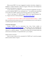
Analysis without covariates
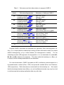
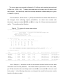
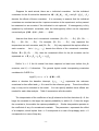
After the setup, doubly click the executable file “CARE-2.exe” to start the program
with the interface shown in Figure 1.
-2-
Figure 1.
The interface of CARE-2 for analysis without covariates.
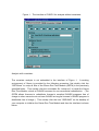
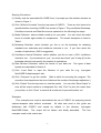
Analysis with covariates
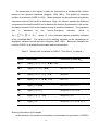
The covariate analysis is not embedded in the interface of Figure 1. A working
environment of Gauss is provided by the following procedure: first doubly click the
“GRTM.exe” to unzip all files of the Gauss Run-Time Module (GRTM) in the previously
specified folder. Then doubly click the executable file “setup.exe” to install the Gauss
Run-Time Module, which is GUASS free-ware for non-commercial redistribution. (The
GRTM allows licensee to redistribute licensee’s compiled GAUSS programs free of
charge to other users who do not have GAUSS so long as licensee’s GAUSS program is
distributed free of charge.) Then doubly click the icon “GSRUN50” on the desktop of
your computer to initialize the Gauss Run-Time Module and then the interface is shown
below.
-3-
Figure 2. The interface of CARE-2 for analysis with covariates.
3. Data Input Format
Data must be read from an ascii file. There are two types of data input formats:
(1) Individual Capture History:
Data are arranged in a matrix, called “individual capture history” matrix, with the rows
representing the capture histories of each captured individual and the columns
representing the captures on each occasion. The capture history of each captured
individual is expressed as a series of 0’s (non-captures) and 1’s (captures) possibly
followed by some individual covariates.
The maximum size for capture history
matrix input in CARE-2 is 2000 individuals and 80 occasions.
(2) Aggregated Categorical Data:
In some studies with many captured individuals, the individual capture history matrix
becomes very large.
It is more convenient to represent the raw data in a categorical
data by a tally of the frequencies of each capture history.
The two types of data input will be illustrated by examples in the following sections.
-4-
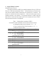
4.
Analysis Without Covariates
Models/Estimators Featured
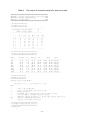
The models considered in CARE-2 are originally proposed in Otis et al. (1978) and
White et al. (1982) and are tabulated in Table 1.
Assume that there are N animals in the
study area and capture-recapture experiments are conducted over t occasions. The
purpose is to estimate the unknown parameter N. Under each model, there are many
available estimators in the literature.
The estimators featured in CARE-2 and their
abbreviations in output (see later sample output for four examples) are shown in Table 2.
All the estimators are shown in the Appendix.
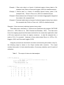
Table 1. Models without covariates in CARE-2.
Pij denotes the capture probability of the ith animal on the jth occasion
pi: heterogeneity effect of the ith individual, i =1, 2, …, N;
ej: time or occasional effect of the jth occasion, j = 1, 2, …, t;
φ: behavioral response effect.
Model
Mtbh
Assumption
⎧ pi e j until first capture
Pij = ⎨
⎩φ pi e j for any recapture
Restriction in model Mtbh
set ej = 1
Mth
⎧ p until first capture
Pij = ⎨ i
⎩φ pi for any recapture
(Generalized removal model)
⎧ e j until first capture
Pij = ⎨
⎩φ e j for any recapture
Pij = pi e j
set φ = 1
Mh
Pij = pi
set ej = 1, φ = 1
Mb
set pi = p, ej = 1
Mt
⎧ p until first capture
Pij = ⎨
⎩φ p for any recapture
(Removal model)
Pij = e j
M0
Pij = p
set pi = p, ej = 1, φ = 1
Mbh
Mtb
-5-
set pi = 1
set pi = 1, φ = 1
Table 2. Estimators and their abbreviations in program CARE-2.
Model
Estimators/Approaches
Estimators in Software CARE-2
M0
Unconditional MLE (UMLE)
Conditional MLE (CMLE)
Estimating equations (EE)
Unconditional MLE (UMLE)
Conditional MLE (CMLE)
Estimating equations (EE)
Unconditional MLE (UMLE)
Conditional MLE (CMLE)
Estimating equations (EE)
Unconditional MLE (UMLE)
Conditional MLE (CMLE)
Estimating equations (EE)
Jackknife (JK1, JK2, IntJK)
Sample coverage (SC1 & SC2)
Estimating equations (EE)
Sample coverage (SC1 & SC2)
Estimating equations (EE)
Jackknife (JK)
Sample coverage (SC)
Estimating equations (EE)
Estimating equations (EE)
Otis et al. (1978)
Darroch (1958)
Yip (1991)
Otis et al. (1978)
Darroch (1958)
Yip (1991)
Otis et al. (1978)
Zippin (1956)
Lloyd (1994)
Chao et al. (2000)
Chao et al. (2000)
Lloyd (1994); Chao et al. (2000)
Burnham and Overton (1978)
Lee and Chao (1994)
Chao et al. (2001)
Lee and Chao (1994)
Chao et al. (2001)
Pollock and Otto (1983)
Lee and Chao (1994)
Chao et al. (2001)
Chao et al. (2001)
Mt
Mb
Mtb
Mh
Mth
Mbh
Mtbh
Program CARE-2 calculates two standard error estimates. One is the asymptotic s.e.
(Asy_s.e. in output) which is obtained by inverting a Fisher information matrix (for models
without heterogeneity) or by a delta method (for heterogeneous models).
For the
estimating equation (EE) approach, the asymptotic s.e. is not obtainable for models Mh,
Mth, Mbh and Mtbh because of complexity. The other method is bootstrap s.e. (Boot_s.e.
in output), which is always obtainable for all estimators.
For interval estimation, CARE-2 provides two 95% confidence intervals based on a
log-transformation method (Chao, 1987) and percentile method (Efron and Tibshirani,
1993) respectively.
Both intervals are constructed from the bootstrap s.e. We remark
that the bootstrap standard error (Boot_s.e.) and confidence intervals may vary from trial
to trial because the bootstrap replication data vary with trials.
-6-
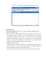
Running Procedures
(1) Doubly click the executable file CARE-2.exe, it prompts you the interface window as
shown in Figure 1.
(2) Click “Without Covariate” from the top menu of CARE-2. There are four items to be
specified before executing CARE-2 as shown in Figure1. They are Model, Bootstrap,
Confidence Interval and Data Structure as explained in the following four steps.
(3) Model Selection: select suitable model(s) for your data. You can check all model
boxes to include eight models for comparisons.
The model description is listed in
Table 1.
(4) Bootstrap Selection: select whether you like to do the bootstrap for obtaining
standard error estimates and confidence intervals or not.
If yes, then select the
number of replications (1000 is suggested).
(5) Confidence Interval Selection: select whether you like to have a 95% confidence
interval or not.
If your selection is “yes”, you must also check “yes” in step (4) for the
bootstrap selection and specify the number of replications.
(6) Data Structure Selection: select the format of your data set.
Two types of data
formats are described in Section 3.
(7) Click “Load Data” to input the filename of your data file (e.g. c:\program
files\CARE-2\data\example1.dat).
(8) Click “Compute” to get the results. (Wait a while for executing the program. The
execution time depends on the size of data and the number of bootstrap replications.)
(9) Click “Output” from the top menu to view the results.
You can click “Save Output” to
save all the output results to a designated file; click “Print” to print the output from
your printer; or click “Clear” to remove all results and to proceed another run.
Examples
Four examples are used to demonstrate the use of CARE-2 for analyzing animal
capture-recapture data without covariates.
All data sets used in this guide are
distributed with CARE-2 and stored by default in the directory c:\program
files\CARE-2\data.
The output will be shown and briefly described.
examples used in this section are:
-7-
The four
Example 1: Deer mice data in a format of individual capture history (data in file:
example1.dat). Refer to Chao and Huggins (2003) for detailed analysis.
Example 2: Mouse data in a format of individual capture history (data in file:
example2.dat).
Refer to Chao et al. (2001) for detailed analysis.
Example 3: Same data set as in Example 2, but in a format of aggregated categorical
form (data in file: example3.dat).
Example 4: Cottontail rabbit data in a format of individual capture history form (data in
file: example4.dat). Refer to Chao et al. (1992) for detailed analysis.
Example 1: Deer mice data (individual capture history data)
These data were collected by V. Reid and are distributed with program CAPTURE
(Otis et al., 1978; White et al., 1982; Rexstad and Burnham, 1991).
The data arose
from a live-trapping experiment that was conducted for six consecutive nights with a total
of 38 mice captured over these six capture occasions.
In data file example1.dat, a
matrix of 38 x 6 is recorded. Analyses of these data include Otis et al. (1978, p. 32),
Huggins (1991) and Chao and Huggins (2003).
Using the procedure as described in the above and selecting all models in step (3),
the following output is shown in the Output window after execution.
The output
contains three parts: (1) basic data information; (2) summary statistics; and (3) results of
estimation.
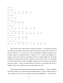
Table 3. The output of deer mice data analysis.
(1) Basic Data Information:
----------------------------------------------Data filename : c:\program files\CARE-2\data\example1.dat
Total # of distinct animals : 38
Number of capture occasions : 6
Bootstrap replications : 1000
----------------------------------------------(2) Summary Statistics:
i
|
u[i]
m[i] n[i]
M[i] ft[i]
f1[i]
--------+-----------------------------------------------1
|
15
0
15
0
9
15
2
|
8
12
20
15
6
11
3
|
6
10
16
23
7
14
4
|
3
16
19
29
6
11
5
|
3
22
25
32
6
8
6
|
3
22
25
35
4
9
7
|
38
-8-
ft[i]: # of individuals that were captured exactly i times on occasions 1, 2, ..., t.
f1[i]: # of individuals that were captured exactly once on occasions 1, 2, ..., i.
(3) Estimation Results:
Model
|
Estimate Boot_s.e.
Asy_s.e.
Phi
CV
95% CI (log-transf.) 95% CI (percentile)
----------------+----------------------------------------------------------------------------------------------M0(CMLE) |
38.5
0.36
0.72
( 38.12, 39.81 )
( 38.13, 39.55 )
M0(UMLE) |
38.0
0.24
0.67
( 38.00, 38.00 )
( 38.00, 38.83 )
M0(EE)
|
38.0
0.36
0.68
( 38.00, 38.00 )
( 38.00, 39.22 )
Mt(CMLE) |
38.4
0.31
0.66
( 38.11, 39.51 )
( 38.08, 39.27 )
Mt(UMLE) |
38.0
0.14
0.62
( 38.00, 38.00 )
( 38.00, 38.53 )
Mt(EE)
|
38.0
0.21
0.62
( 38.00, 38.00 )
( 38.00, 38.73 )
Mb(CMLE) |
42.3
7.30
3.75
1.92
( 38.43, 80.28 )
( 38.77, 57.41 )
Mb(UMLE) |
40.8
6.91
3.05
1.79
( 38.18, 81.43 )
( 38.00, 51.98 )
Mb(EE)
|
41.9
5.29
3.58
1.89
( 38.53, 66.84 )
( 38.00, 53.28 )
Mh(SC1) |
43.5
3.81
3.72
0.50
( 39.64, 56.78 )
( 39.65, 50.94 )
Mh(SC2) |
42.4
3.52
3.40
0.48
( 39.09, 55.48 )
( 38.73, 49.29 )
Mh(JK1) |
45.5
3.58
3.71
( 41.09, 56.22 )
( 41.33, 49.67 )
Mh(JK2) |
48.3
5.78
5.68
( 41.69, 66.72 )
( 39.73, 57.83 )
Mh(IntJK) |
45.5
8.35
3.71
( 39.29, 81.58 )
( 41.33, 70.24 )
Mh(EE)
|
40.2
2.14
---0.50
( 38.44, 48.89 )
( 38.00, 43.76 )
Mtb(CMLE) |
48.0
12.78
11.98
2.95
( 39.46,106.76 )
( 38.78, 85.55 )
Mtb(UMLE) |
43.6
11.12
6.90
2.34
( 38.47,104.74 )
( 38.07, 80.31 )
Mtb(EE) |
47.1
8.51
10.78
2.82
( 39.91, 81.09 )
( 38.00, 68.25 )
Mth(SC1) |
43.6
3.97
3.77
0.51
( 39.62, 57.57 )
( 39.70, 51.76 )
Mth(SC2) |
42.5
3.41
3.45
0.49
( 39.18, 54.85 )
( 38.90, 48.89 )
Mth(EE) |
40.3
2.20
---0.51
( 38.48, 49.14 )
( 38.00, 44.26 )
Mbh(SC) |
50.5
23.43
---0.60
( 39.13,176.57 )
( 38.89,125.72 )
Mbh(JK) |
53.0
9.43
---( 42.84, 84.47 )
( 38.00, 73.00 )
Mbh(EE) |
43.5
4.44
---1.68
0.40
( 39.36, 60.04 )
( 38.00, 51.33 )
Mtbh(EE) |
44.2
4.58
---1.89
0.36
( 39.72, 60.60 )
( 38.10, 53.58 )
----------------+-----------------------------------------------------------------------------------------------
The first part of the output shows basic information including the data filename,
(c:\program files\CARE-2\data\example1.dat for this example), the number of distinct
animals caught in the experiment (38 in this case), the number of trapping occasions (6
in this case) and the number of bootstrap replications (1000 in this case).
The summary statistics are listed in the second part of the output.
We use these
data to introduce some notation. The numbers of captures for the six occasions are (n1,
n2, ..., n6) = (15, 20, 16, 19, 25, 25). Out of the nj animals, there are uj first-captures and
mj recaptures, so that uj + mj = nj, with (u1, u2, ..., u6) = (15, 8, 6, 3, 3, 3) and (m1, m2, ...,
m6) = (0, 12, 10, 16, 22, 22). The statistic Mj denotes the number of marked animals
just before the jth occasion.
Thus Mj = u1 + u2 + …+ uj-1 and (M1, M2, ..., M7) = (0, 15,
23, 29, 32, 35, 38) for these data. That is, the number of marked individuals in the
population progressively increased from M1 = 0 to M7 = 38.
Here Mt+1 denotes the total
number of distinct animals caught in the experiment. The frequency counts for the six
occasions are (f16, f26, ..., f66) = (9, 6, 7, 6, 6, 4), where fjk denotes the number of animals
-9-
captured exactly j times on occasions 1, 2, …, k. Since singleton information is usually
important, we also list (f11, f12, …, f16) = (15, 11, 14, 11, 8, 9).
The third part shows estimation results.
For these data, Otis et al. (1978, p. 32)
indicated that the most suitable model for these data was model Mb. Based on the
usual unconditional MLE approach, Mb(UMLE) in Table 3, the estimated population size
in model Mb is 41 with bootstrap s.e. of 6.9 and asymptotic s.e. of 3.1. The 95%
confidence intervals are (38.2, 81.4) and (38.0, 52.0) for log-transformation and
percentile methods respectively based on the bootstrap procedure.
The proportion
constant between the re-capture probability and first-recapture probability (φ in Table 1 or
Phi in Table 3) is estimated to be 1.79, suggesting animals became trap-happy after their
first capture.
Chao and Huggins (2003) suggested considering further general models Mbh and
Mtbh by use of estimating equation (EE) approach.
estimates, Mbh(EE) and Mtbh(EE) in Table 3.
The two models produce close
So it is reasonable to adopt the most
general model Mtbh and conclude that the population size is about 44 (standard error 4.6).
The data based on model Mtbh show strong trap-happy behavior (Phi = 1.89 in Table 3), a
low degree of heterogeneity (the CV estimate is 0.36, where CV denotes the coefficient
of variation of {p1, p2, …, pN), and slight time-varying effects as the relative time effects
are estimated to be ( p e1 , p e2 , ..., p e6 ) = (0.34, 0.32, 0.26, 0.26, 0.33, 0.33), where p
denotes the average of pi’s. (Time effects are not shown in the output. Refer to Chao
et al. 2001 for calculation formula.)
The 95% confidence interval using a log-transformation under model Mtbh is 40 to
61.
This interval is unavoidably wider than that for model Mb because more parameters
are involved.
Usually, a simpler model has smaller variance but larger bias whereas a
general model has lower bias but larger variance. For interval estimation, a simpler
model produces narrow confidence interval with possibly poor coverage probability
whereas a more general model produces wide interval with more satisfactory coverage
probability.
A trade-off clearly occurs with this example.
Example 2: Mouse data (individual capture history)
- 10 -
The mouse data were originally collected by S. Hoffman and described and analyzed
in Otis et al. (1978, p. 93). Trapping was conducted on five days and 110 distinct mice
were caught.
We specifically select this example because a detailed analysis is given
in Chao et al. (2001).
For this data set, since Otis et al. (1978) concluded that for these data behavior is
the strongest factor affecting capture probabilities, we select three models with
behavioral response (models Mb, Mtb and Mtbh) in step (3) of the procedures presented
earlier.
The results are the following:
Table 4. The output of mouse data analysis.
(1) Basic Data Information:
-----------------------------------------------------------Data filename
: c:\program files\CARE-2\data\example2.dat
Total distinct animals
: 110
Number of capture occasions : 5
Bootstrap replications
: 1000
-----------------------------------------------------------(2) Summary Statistics:
i
|
u[i]
m[i]
n[i]
M[i]
ft[i] f1[i]
--------+-----------------------------------------------1
|
37
0
37
0
34
37
2
|
31
23
54
37
20
45
3
|
9
49
58
68
28
27
4
|
21
44
65
77
15
38
5
|
12
57
69
98
13
34
6
|
110
ft[i]: # of individuals that were captured exactly i times on occasions 1, 2, ..., t.
f1[i]: # of individuals that were captured exactly once on occasions 1, 2, ..., i.
(3) Estimation Results:
Model
|
Est.
Boot_s.e.
Asy_s.e.
Phi
CV
95%CI(log-transf.) 95%CI(percentile)
-------------------+----------------------------------------------------------------------------------Mb(CMLE)
|
145.5
25.40
18.02
2.51
( 120.09,235.16 )
( 124.23,214.34 )
Mb(UMLE)
|
142.2
22.68
16.42
2.42
( 119.28,221.72 )
( 122.92,206.70 )
Mb(EE)
|
139.9
21.84
15.37
2.36
( 118.32,217.71 )
( 120.80,195.35 )
Mtb(CMLE)
|
173.7
46.20
55.69
3.63
( 127.83,337.77 )
( 123.85,293.48 )
Mtb(UMLE)
|
161.1
42.71
41.72
3.19
( 122.25,322.82 )
( 121.45,285.52 )
Mtb(EE)
|
152.0
28.68
32.87
2.87
( 122.46,251.21 )
( 118.99,224.05 )
Mtbh(EE)
|
123.2
11.75
---1.03
0.52
( 112.95,169.00 )
( 113.51,156.30 )
--------------------+--------------------------------------------------------------------------------
As in Example 1, estimation results for the selected models follow the basic data
information and summary statistics. The model selection procedure in Otis et al. (1978,
pp. 92-96) shows that the most likely model is model Mtbh and model Mb is the next most
likely model.
In the following discussion, we interpret the results for these two models
based on the above output.
- 11 -
The unconditional MLE for model Mb , Mb(UMLE) in Table 4, yields an estimate of
142.2 with an asymptotic s.e. of 16.42 and a bootstrap s.e. of 22.68. A 95% confidence
interval constructed by a log-transformation is in the range of (119, 222); the bootstrap
percentile method gives an interval range of (123, 207).
The ratio of recapture and
first-capture probabilities, φ, is estimated to be 2.42 (Phi = 2.42 in the output), which
shows a trap-happy situation. The conditional MLE estimate is 145.5 and the estimate
based on an optimal estimating equation is 139.9.
Their associated variance and
confidence intervals are shown in the above output.
If model Mtbh is assumed, an estimating equation approach (Chao et al., 2001)
yields an estimate of 123 with an estimated bootstrap s.e. of 11.75.
A 95% confidence
interval associated with this estimate under model Mtbh is (113, 169) or (114, 156) based
on two methods.
Example 3: Mouse data (aggregated categorical data)
In Example 2, we used the mouse data with individual capture history.
Example3.dat files the data in a format of aggregated categorical data. The user can
view Example3.dat for the required format for CARE-2. All running procedures are
similar to those in Examples 1 and 2 except that aggregated categorical data is selected
in step (6).
The output is exactly the same as that in Example 2 except for the bootstrap
s.e. and confidence intervals.
Example 4: Cottontail rabbit data (individual capture history)
Edwards
and
Eberhardt
(1967)
conducted
an
18
trapping-occasion
capture-recapture experiment on a confined population of known size.
In their study,
135 wild cottontail rabbits were penned in a 4-acre rabbit-proof enclosure.
captures, there were 76 distinct rabbits.
Out of 142
An advantage of this data set is the true
population size is known. The basic data information and the summary statistics are
shown in Table 5.
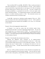
Otis et al. (1978, pp. 84-87) found that for these data there was significant time
variation and heterogeneity but little behavioral response. Hence we select all models
with time and/or heterogeneity (models Mt, Mh and Mth) along with the most general
- 12 -
model Mtbh. This data was analyzed in the literature (e.g. Burnham and Overton, 1978;
Chao et al., 1992). This data set with individual capture history is filed in “example4.dat”.
The output for models Mt, Mh and Mth is given in Table 5.
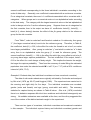
Table 5.
The output of cottontail rabbit data analysis.
(1) Basic Data Information:
-----------------------------------------------------------Data filename
: c:\program files\CARE-2\data\example4.dat
Total distinct animals
: 76
Number of capture occasions : 18
Bootstrap replications : 1000
-----------------------------------------------------------(2) Summary Statistics:
i
|
u[i]
m[i]
n[i]
M[i]
ft[i] f1[i]
--------+-----------------------------------------------1
|
9
0
9
0
43
9
2
|
6
2
8
9
16
13
3
|
3
6
9
15
8
12
4
|
11
3
14
18
6
22
5
|
4
4
8
29
0
24
6
|
1
4
5
33
2
23
7
|
10
8
18
34
1
29
8
|
7
4
11
44
0
35
9
|
1
3
4
51
0
35
10
|
1
2
3
52
0
35
11
|
9
7
16
53
0
43
12
|
0
5
5
62
0
41
13
|
1
1
2
62
0
41
14
|
5
2
7
63
0
46
15
|
6
3
9
68
0
50
16
|
0
0
0
74
0
50
17
|
0
4
4
74
0
47
18
|
2
8
10
74
0
43
19
|
76
ft[i]: # of individuals that were captured exactly i times on occasions 1, 2, ..., t.
f1[i]: # of individuals that were captured exactly once on occasions 1, 2, ..., i.
(3) Estimation Results
Model
|
Est.
Boot_s.e.
Asy_s.e.
Phi
CV
95%CI(log-transf.) 95%CI(percentile)
----------------------+----------------------------------------------------------------------------------Mt(CMLE)
|
96.0
8.13
6.70
( 85.27,119.04 )
( 86.63,112.19 )
Mt(UMLE)
|
95.1
8.36
6.58
( 84.39,119.37 )
( 85.98,110.34 )
Mt(EE)
|
95.0
8.81
6.57
( 83.97,121.10 )
( 85.46,112.73 )
Mh(SC1)
|
137.0
21.50
21.44
0.67
( 107.20,195.31 )
( 106.43,182.11 )
Mh(SC2)
|
132.8
22.05
20.62
0.65
( 103.26,194.39 )
( 103.47,181.51 )
Mh(JK1)
|
116.6
8.54
8.89
( 103.01,137.07 )
( 107.17,125.11 )
Mh(JK2)
|
141.4
14.25
14.87
( 118.92,175.79 )
( 120.76,162.13 )
Mh(IntJK)
|
142.3
38.07
15.18
( 99.27,264.74 )
( 107.17,252.17 )
Mh(EE)
|
125.3
16.41
---0.67
( 102.15,169.10 )
( 100.39,154.64 )
Mth(SC1)
|
138.9
24.35
22.05
0.70
( 106.23,206.84 )
( 108.82,194.47 )
Mth(SC2)
|
134.6
22.56
21.22
0.68
( 104.29,197.46 )
( 105.93,183.40 )
Mth(EE)
|
-***-------------Mtbh(EE)
|
-***----------------------------------------+----------------------------------------------------------------------------------*** iterative steps do not converge
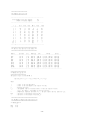
Edwards and Eberhardt (1967) reported that the usual estimators based on
equal-catchability considerably underestimated the true number 135.
It is readily seen
from the output that all estimates based on model Mt, Mt(CMLE), Mt(UMLE) and Mt(EE)
in the output, are about 95 or 96. Burnham and Overton (1978) suggested modeling
- 13 -
these data by model Mh and adopted an interpolated jackknife estimator. In the output,
the first-order, Mh(JK1), and the second-order jackknife, Mh(JK2), are also shown; the
interpolated jackknife, Mh(IntJK) yields an estimate of 142 with an asymptotic s.e. of
15.18.
The confidence interval proposed by Burnham and Overton (1978) was (112,
172) based on the asymptotic s.e.
This interval is different from ours in Table 5
because we use a bootstrap s.e. The asymptotic s.e. is also tabulated so that user can
compute relevant intervals.
If model Mth is assumed, the coefficient of variation (CV) of the capture probabilities
for all estimation methods is estimated to be about 0.70 as shown in the output. This
relatively large value of the CV gives strong evidence of heterogeneity because the CV =
0 corresponds to no heterogeneity.
The two estimators using the sample coverage
methods, Mth(SC1) and Mth(SC2), proposed by Chao et al. (1992) and Lee and Chao
(1994) are respectively 138.9 (s.e. 24.35) and 134.6 (s.e. 22.56). The latter gives a
95% confidence interval (104, 197) using a log-transformation and (106, 183) using a
percentile method. The estimating equation approach does not yield an estimate due to
insufficient capture and recapture information, which causes failure of convergence in
the numerical iterations.
arises.
If we adopt the most general model Mtbh, similar difficulty
Therefore, capture and recapture information is not sufficient for fitting a
complicated model with three sources of variations.
We caution that in some cases,
estimates can still be obtained in the case of insufficient information, but the standard
error generally becomes so large that the model is useless.
5.
Analysis With Covariates
Models/Estimators Featured
In program CARE-2, we distinguish covariates as two types: individual covariates
and occasional covariates as in Huggins (1989, 1991).
Individual covariates include
individual’s characteristics (age, sex, body weight or wing length) and occasional
covariates could be environmental variables (temperature on each occasion) or known
catch-effort expended in trapping method (e.g., number of traps on each capture
occasion).
Occasional covariates should be stored in another file as will be shown in
Example 6 below.
- 14 -
Suppose for each animal, there are s individual covariates.
Let the individual
covariates for the ith animal be denoted as Wi ′ = (Wi 1,Wi 2 ,...,Wis ) and β ′ = (β1,β 2 ,...,β s )
denotes the effects of these covariates.
It is necessary to assume that the individual
covariates are constant across the t capture occasions in the experiment, as they cannot
be measured on an occasion if the individual is not captured.
If heterogeneity is fully
explained by individuals’ covariates, then the heterogeneity effect can be expressed
conveniently as β ′ Wi = β1Wi 1 + β 2Wi 2 + ... + β sWis .
Assume that there are b occasional covariates: {R11, R12, …, R1t}, {R21, R22, …,
R2t}, …, {Rb1, Rb2, …, Rbt}.
For example, {R11, R12, …, R1t}
may represent the
temperature on each occasion, and {Rb1, Rb2, …, Rbt} may represent the capture effort on
each occasion.
Let r ′ = (r1, r2 ,...,rb ) denote the effects of the occasional covariates.
Define R ′j = {R1j, R2j, …, Rbj}, then the occasional effect for the jth occasion can be
expressed as r ′ R j = r1R1j + r2 R2j +…+ rbRbj.
Define Yij = 1 if the ith animal has been captured at least once before the jth
occasion, and Yij = 0 otherwise. The general logistic model incorporating covariates
considered in CARE-2 is
logit(Pij ) = a + c j + v Yij + β ′ Wi + r ′ R j ,
where a denotes the baseline intercept, {c1,c2, …,ct-1} represents the unknown
occasional or time effect and ct ≡ 0 is used for the reference group. These time effects
may or may not be included in the model. You can specify whether these effects are
needed for each data analysis. Table 6 summarizes all sub-models.
The interpretation of the coefficient of any β is based on the fact that when β > 0, the
larger the covariate is, the larger the capture probability is, while if β < 0 then the larger
the covariate is, the smaller the capture probability is. Similar interpretation pertains to
the coefficient of any r for occasional covariate. The parameter v represents the effect
of a recapture, which implies that v > 0 corresponds to a case of trap-happy and v < 0
corresponds to a case of trap-shy.
- 15 -
The parameters in the logistic models are estimated by a conditional ML method
based on the captured individuals (Huggins, 1989, 1991). The default of maximum
number of iterations in CARE-2 is 500. Model selection can be performed using Akaike
information criterion (AIC) which is defined as -2logL+2m, where L denotes the likelihood
computed at the conditional MLE and m denotes the number of parameters in the model.
A model is selected if AIC is the smallest among all models considered. The population
size
is
estimated
by
the
Horvitz-Thompson
estimator,
which
is
−1
M
t
Nˆ HT = ∑i =t1+1 {1 − ∏ j =1(1 − Pˆij )} , where Pˆij is the estimated capture probability evaluated
at the conditional MLE. The variance of the resulting estimator can be estimated by an
asymptotic variance formula derived in Huggins (1989, 1991). Below two examples are
used for CARE-2 to illustrate the estimation and model selection.
Table 6. Models with covariates in CARE-2. (The effect cj is optional.)
Model
Restriction in model M*tbh
Assumption
M*tbh
logit(Pij ) = a + c j + v Yij + β ′ Wi + r ′ R j
M*bh
logit(Pij ) = a + v Yij + β ′ Wi
set cj = 0, r = 0
M*tb
logit(Pij ) = a + c j + v Yij + r ′ R j
set β = 0
M*th
logit(Pij ) = a + c j + β ′ Wi + r ′ R j
set v = 0
M *h
logit(Pij ) = a + β ′ Wi
set cj = 0, r = 0, v = 0
M *b
logit(Pij ) = a + v Yij
set β = 0, cj = 0, r = 0
M *t
logit(Pij ) = a + c j + r ′ R j
set β = 0, v = 0
M *0
logit(Pij ) = a
set β = 0, cj = 0, r = 0, v = 0
Running Procedures by Examples
In the following, we provide two examples to demonstrate the procedure of CARE-2
- 16 -
for covariate analysis.
They are:
Example 5: Same capture data as in Example 1, but three individual covariates are
included (data in file: example5.dat). Refer to Huggins (1991) and Chao
and Huggins (2003) for detailed analysis.
Example 6: Rodent data with two individual covariates and one occasional covariate
(capture data and individual covariates are in file: exampl61.dat;
occasional data are in file: exampl62.dat). Refer to Huggins (1989) for
detailed analysis.
Example 5: Deer mice data (with three individual covariates)
For the data set discussed in Example 1, there were actually three covariates:
gender (male or female), age (young, semi-adult or adult) and weight, collected for each
individual in the deer mouse data. Only three semi-adult mice were caught, so they
were re-classified as adults. The user can view example5.dat for the complete data.
Part of the complete data is shown in Table 7.
Table 7. Individual capture history of deer mice with three covariates: Gender (0:
male, 1: female); Age (y: young, a: adult); and Weight (in grams).
Occasion 1 Occasion 2 Occasion 3 Occasion 4 Occasion 5 Occasion 6
Gender
Age
Weight
1
1
1
1
1
1
0
y
12
1
0
0
1
1
1
1
y
15
1
‧
‧
‧
1
0
0
1
‧
‧
‧
1
0
y
15
‧
‧
‧
0
0
0
0
0
0
0
0
0
0
1
1
0
1
a
a
16
19
There are three individual covariates and there is no occasional covariate. Since
every covariate can be treated as either categorical or continuous, the user has to
specify the numbers of each.
For example, there are two categorical (gender and age)
and one continuous (weight) for individual covariates of this data. In the data format,
the order of data entry should be: capture history, categorical covariates followed by the
continuous covariates. Occasional covariates are stored in a separate file with the
- 17 -
same order of categorical variables first and then continuous variables.
We describe the procedures for analyzing deer mice data with covariates. The
following procedure must be executed in a GAUSS environment.
(1) Provoke GAUSS environment either by doubly clicking GSRUN50 on your desktop
as described in Download and Setup or by clicking the executable file GSRUN.exe
stored in the directory GSRUN50.
(2) Click “File” on the top menu of GAUSS and subsequently click “Run Program” and
select the program CARE-2.gcg which is stored in a pre-specified working directory
(The default is c:\program files\CARE-2\). It prompts you subsequently the following
input steps:
(3) “Please input the number of distinct individuals:” In this example, we input 38.
(4) “Please input the number of sampling occasions:” Input 6.
(5) “Please input the number of categorical individual covariates:” Input 2.
(6) “Please input the number of continuous individual covariates:” Input 1.
(7) “Please input the filename containing the capture history and individual covariates
(continuous type covariates must follow by the categorical type covariates):” Input
c:\program files\CARE-2\data\example5.dat.
(8) “Please input the number of categorical occasional covariates:” Input 0.
(9) “Please input the number of continuous occasional covariates:”
Input 0.
(10) “Do you want to include the unknown time effects (y or n)?” (This means that
whether the effects {c1,c2, …,ct-1} are needed in the logistic model). We input y.
(11) “Please input the filename to save the output:” Input for example c:\program
files\CARE-2\output.out. Please wait a moment and the results will be shown in
the GAUSS window. Moreover, the output is also saved in c:\program
files\CARE-2\output.out. The standard output for CARE-2 with this example with
the above input is shown in Table 8.
Remark: If you have abundant data, it may take a long time to get your output due to
complicated iterative estimation in GAUSS program operating on a large array or
high-dimensional matrix.
- 18 -
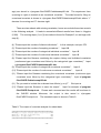
Table 8. The output of covariate analysis for deer mice data.
#############################################################
### CARE-2 for capture-recapture analysis with covariates ###
### Authors: Anne Chao and Hsin-Chou Yang
###
### Version: 1.5 (April 2006)
###
#############################################################
==========================
=== Summary Statistics ===
==========================
-----------------------------------------------------Total number of distinct animals :
38
Number of capture samples :
6
-----------------------------------------------------i
|
u[i]
m[i] n[i]
M[i]
ft[i]
f1[i]
--------|---------------------------------------------1
|
15
0
15
0
9
15
2
|
8
12
20
15
6
11
3
|
6
10
16
23
7
14
4
|
3
16
19
29
6
11
5
|
3
22
25
32
6
8
6
|
3
22
25
35
4
9
7
|
38
--------|---------------------------------------------==========================================
=== The Fit & Estimation of all models ===
==========================================
Model
Estimate
S.E.
MIN(-LL)
AIC
95% CI
Status
----------------------------------------------------------------------------------M*0
38.47
0.72
157.27
316.54
(38.06, 42.04) Converge
M*t
38.40
0.66
152.42
316.84
(38.04, 41.80) Converge
M*b
42.25
3.76
150.43
304.87
(38.96, 56.86) Converge
M*h
39.85
1.72
144.87
297.75
(38.39, 46.67) Converge
M*tb
46.48
12.65
148.18
310.36
(39.02, 108.74) Converge
M*th
39.66
1.61
139.55
297.10
(38.34, 46.20) Converge
M*bh
47.15
7.17
139.54
289.09
(40.35, 73.52) Converge
M*tbh
47.13
10.08
137.33
294.66
(39.59, 90.50) Converge
-----------------------------------------------------------------------------------=========================
=== Model Description ===
=========================
The general logistic model M*tbh is
logit(P_ij)=a + c_j + v * Y_ij + beta * W_i + r * R_j
where
i
j
a
c_j
v
beta
r
:
:
:
:
refers to the ith individual;
refers to the jth sample or jth capture occasion;
baseline intercept;
the unknown time or occasional effect of the jth capture occasion
(set c_t=0, where t: the number of capture occasions;
: (behavioral response) the effect w.r.t. the past capture history indicator Y_ij;
: the effect of individual covariates W_i;
: the effect of occasional covariate R_j;
===========================================
=== The MLEs of Regression Coefficients ===
===========================================
*** Model M*0 ***
a
- 19 -
MLE
S.E.
0.08
0.13
*** Model M*t ***
a
c_1
MLE
0.62
-1.07
S.E.
0.24
0.42
c_2
-0.54
0.42
c_3
-0.96
0.42
c_4
-0.64
0.42
c_5
0.00
0.17
*** Model M*h ***
a
beta1(1)
MLE
-1.95
0.81
S.E.
0.71
0.31
beta2(1)
-1.90
0.57
beta3
0.16
0.06
*** Model M*tb ***
a
v
MLE
-1.16
1.72
S.E.
1.09
0.98
c_1
0.42
0.80
c_2
0.31
0.57
c_3
-0.45
0.49
c_4
-0.37
0.45
c_5
0.12
0.42
beta3
0.16
0.06
c_1
-1.18
0.44
c_2
-0.59
0.43
c_3
-1.06
0.44
c_4
-0.70
0.43
c_ 5
0.00
0.19
c_1
-0.11
0.87
c_2
0.02
0.80
c_3
-0.71
0.60
c_4
-0.50
0.56
*** Model M*b ***
a
v
MLE
-0.76
1.22
S.E.
0.34
0.38
*** Model M*th ***
a
beta1(1)
MLE
-1.43
0.84
S.E.
0.74
0.32
beta2(1)
-1.98
0.58
*** Model M*bh ***
a
v
MLE
-2.91
1.18
S.E.
0.87
0.40
beta1(1)
0.92
0.35
beta2(1)
-1.88
0.63
beta3
0.16
0.06
*** Model M*tbh ***
a
v
MLE
-2.76
1.21
S.E.
1.30
0.74
beta1(1)
0.94
0.36
beta2(1)
-1.92
0.64
beta3
0.16
0.06
c_5
0.08
0.57
The first part of the output shows all summary statistics. The second part shows
the fitting and estimation results for the logistic model and all sub-models, followed by
model description.
For each model, the corresponding estimated population size
(number under the heading Estimate in Table 8), its s.e. (under the heading S.E.),
negative value of the minimum log-likelihood under the heading MIN(-LL), the Akaike
information criterion (AIC) and 95% confidence interval (Chao, 1987) are calculated.
From the values of AIC, we select model M*bh because AIC of this model is the smallest
among all models. There are slight differences between our estimates and those in
Huggins (1991) because different numerical algorithms are used.
The last part of the output shows all fitted parameter estimates. Under model M*bh,
the fitted intercept is -2.91, the behavioral response effect is 1.18 for re-capture (the first
capture effect is set to be 0, so recaptures have higher probabilities). Then there are
- 20 -
several coefficients corresponding to the three individual’s covariates according to the
order of data entry. Generally, one coefficient is associated with a continuous covariate.
For a categorical covariate, there are k-1 coefficients associated with a covariate with k
categories. When groups are in a numerical order or in an alphabetical order according
to the data entry. The category with the largest numerical value or the last alphabetical
order is always set to be 0 as the reference group.
Suppose there are k categories for
the first covariate, then in the output we have k-1 coefficients: beta1(1), beta1(2), …,
beta1(k-1), where betan(j) denotes the effect of the jth group relative to the reference
group for the nth covariate.
From Table 7, male is coded as 0 and female is coded as 1 in data entry, thus group
“1” (the larger numerical value) is set to be the reference group. Therefore, in Table 8,
the coefficient, beta1(1) = 0.92, is the effect for male; the female is set to be 0, so males
have larger probabilities. Also, young is coded as “y” and adult is coded as “a” in data
entry, thus in an alphabetical order the group “y” is used for reference group. The
second coefficient, beta2(1) = -1.88, is the effect for adult; the young effect is set to be 0,
so young have larger capture probabilities.
The last coefficient in the output, beta3 =
0.16 is the effect for a unit change of body weight. This implies the heavier the weight,
the larger the capture probability.
Then from the summary of model fitting the estimated
population size under the selected model M*bh is 47.2 (s.e. 7.17) with a 95% confidence
interval of (40.4, 73.5).
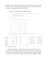
Example 6: Rodents data (two individual covariates and one occasional covariate).
The data of salt marsh rodents were originally collected by Coulombe and analyzed
by Otis et al. (1978, pp. 62-67) and Huggins (1989). The experiment was carried out in
the morning and night daily for five days.
Two individual covariates are recorded:
gender (male and female) and age (young, semi-adult and adult).
The summary
statistics for capture history are shown in Table 9 below. Otis et al. (1978) concluded
there is no behavior response effect but time variations and individual heterogeneity are
strong. No suitable estimators were available at the time, and thus they suggested the
use of the number of the distinct animals caught in the experiment.
There are two types of covariates, individual covariates and occasional covariates
in this example. The individual capture history and individual covariates (gender and
- 21 -
age) are stored in c:\program files\CARE-2\data\exampl61.dat. The experiment time
(morning or night) is treated as an occasional covariate. The data format for filing an
occasional covariate is shown in c:\program files\CARE-2\data\exampl62.dat, where “1”
denotes for morning and “2” denotes night.
There are two rodents with missing covariates, hence we exclude these two records
in the following analysis. It leads to somewhat different results from those in Huggins
(1989). The running steps (1) to (3) are similar to those for Example 5, so we begin with
step (4).
(4) “Please input the number of distinct individuals:”. In this example, we input 171.
(5) “Please input the number of sampling occasions:”. Input 10.
(6) “Please input the number of categorical individual covariates:”. Input 2.
(7) “Please input the number of continuous individual covariates:”. Input 0.
(8) “Please input the filename containing the capture history and individual covariates
(continuous type covariates must follow by the categorical type covariates):” Input
c:\program files\CARE-2\data\exampl61.dat.
(9) “Please input the number of categorical occasional covariates:”. Input 1.
(10) “Please input the number of continuous occasional covariates:”.
Input 0.
(11) “Please input the filename containing the occasional covariates (continuous type
covariates must follow by the categorical type covariates):”.
Input c:\program
files\CARE-2\data\exampl62.dat.
(11) “Do you want to include the unknown time effects (y or n)?”. We input n.
(12) “Please input the filename to save the output:”. Input for example c:\program
files\CARE-2\output.out. Please wait a moment and the results will be shown in
the GAUSS window. Moreover, the output is also saved in c:\program
files\CARE-2\output.out. The standard output is shown in Table 9.
Table 9. The output of covariate analysis for rodent data.
#############################################################
### CARE-2 for capture-recapture analysis with covariates ###
### Authors: Anne Chao and Hsin-Chou Yang
###
### Version: 1.5 (April 2006)
###
#############################################################
- 22 -
==========================
=== Summary Statistics ===
==========================
-----------------------------------------------------Total number of distinct animals :
171
Number of capture samples :
10
-----------------------------------------------------i
|
u[i]
m[i] n[i]
M[i]
ft[i]
f1[i]
--------|---------------------------------------------1
|
68
0
68
0
2
68
2
|
33
27
60
68
62
74
3
|
26
36
62
101
40
74
4
|
12
40
52
127
31
65
5
|
15
58
73
139
16
54
6
|
3
38
41
154
13
45
7
|
12
64
76
157
5
41
8
|
0
35
35
169
1
26
9
|
2
74
76
169
0
9
10
|
0
38
38
171
1
2
11
|
171
--------|---------------------------------------------==========================================
=== The Fit & Estimation of all models ===
==========================================
Model
Estimate
S.E.
MIN(-LL)
AIC
95% CI
Status
----------------------------------------------------------------------------------M*0
173.99
1.83
1093.07 2188.14
(171.99, 180.02)
Converge
M*t
173.79
1.76
1071.43 2146.86
(171.90, 179.68)
Converge
M*b
172.99
1.60
1092.39 2188.78
(171.50, 178.96)
Converge
M*h
175.38
2.33
1080.36 2168.72
(172.65, 182.64)
Converge
M*tb
173.74
1.74
1071.43 2148.86
(171.87, 179.57)
Converge
M*th
175.14
2.26
1058.44 2126.89
(172.52, 182.26)
Converge
M*bh
173.86
2.05
1079.44 2168.87
(171.81, 181.09)
Converge
M*tbh
174.86
2.21
1058.42 2128.84
(172.36, 181.95)
Converge
-----------------------------------------------------------------------------------=========================
=== Model Description ===
=========================
The general logistic model M*tbh is
logit(P_ij)=a + c_j + v * Y_ij + beta * W_i + r * R_j
where
i
j
a
c_j
v
beta
r
:
:
:
:
refers to the ith individual;
refers to the jth sample or jth capture occasion;
baseline intercept;
the unknown time or occasional effects of the jth capture occasion
(set c_t=0, where t: the number of capture occasions;
: (behavioral response) the effect w.r.t. the past capture history indicator Y_ij;
: the effect of individual covariates W_i;
: the effect of occasional covariate R_j;
===========================================
=== The MLEs of Regression Coefficients ===
===========================================
*** Model M*0 ***
a
MLE
-0.69
S.E.
0.05
- 23 -
*** Model M*t ***
a
r1(1)
MLE
0.31
-0.68
S.E.
0.16
0.10
*** Model M*b ***
a
v
MLE
-0.58
-0.15
S.E.
0.10
0.11
*** Model M*h ***
a
beta1(1)
MLE
-0.38
-0.28
S.E.
0.08
0.11
beta2(1)
-0.02
0.13
*** Model M*tb ***
a
v
MLE
0.31
-0.01
S.E.
0.16
0.00
r1(1)
-0.67
0.10
*** Model M*th ***
a
beta1(1)
MLE
0.63
-0.28
S.E.
0.17
0.11
beta2(1)
-0.02
0.14
*** Model M*bh ***
a
v beta1(1)
MLE
-0.24
-0.18
-0.28
S.E.
0.12
0.13
0.11
*** Model M*tbh ***
a
v
MLE
0.65
-0.03
S.E.
0.16
0.05
beta1(1)
-0.28
0.11
beta2(2)
-0.46
0.11
beta2(2) r1(1)
-0.47
-0.68
0.12
0.11
beta2(1)
-0.02
0.14
beta2(1)
-0.02
0.15
beta2(2)
-0.46
0.11
beta2(2) r1(1)
-0.47
-0.68
0.12
0.11
From the results of AIC listed in Table 9, model Mth is selected. The conclusion is
consistent with that in Otis et al. (1978, pp. 62-64). For gender (data entry is 1 for male
and 2 for female), the female is served as the reference group.
The negative
regression coefficient beta1(1) = -0.28 demonstrates that the females have larger
capture probabilities than the males. For age (data entry is 1 for young, 2 for semi-adult
and 3 for adult), thus the adult group with the largest numerical value is regarded as a
reference group. The regression coefficient beta2(1) = -0.02 is not significant, hence
there is no significantly difference of capture probabilities between the young and adult.
However, the regression coefficient beta2(2) = -0.47 is significantly different from 0,
which implies that adults have higher capture probabilities than the semi-adult. For the
occasional covariate (data entry is 1 for morning and 2 for night), the coefficient r1(1) =
-0.68 denotes the effect of morning time.
Thus the capture probabilities are higher in
the night. The population size estimate under model Mth is 175.1 with an estimated s.e.
of 2.3 and a 95% confidence interval of (172.5, 182.3). These results here are slightly
different from those obtained in Huggins (1989) due to the different ways of treating
missing covariates.
- 24 -
Reference
Burnham, K.P. and Overton, W.S. (1978). Estimation of the size of a closed population
when capture probabilities vary among animals. Biometrika 65, 625-33.
Chao, A. (1987). Estimating the population size for capture-recapture data with unequal
catchability. Biometrics 43, 783-91.
Chao, A., Chu, W. and Hsu, C.-H. (2000). Capture-recapture when time and behavioral
response affect capture probabilities. Biometrics 56, 427-33.
Chao, A. and Huggins, R.M. (2003). Closed population models. To appear as a chapter
in The Handbook of Capture-Recapture Methods. Edited by Manly, B., McDonald, T.
and Amstrup, S. Princeton University Press.
Chao, A., Lee, S.-M. and Jeng, S.-L. (1992). Estimating population size for
capture-recapture data when capture probabilities vary by time and individual
animal. Biometrics 48, 201-16.
Chao, A., Yip, P.S.F., Lee, S.-M. and Chu, W. (2001). Population size estimation based
on estimating functions for closed capture-recapture models.
Journal of Statistical
Planning and Inference 92, 213-32.
Darroch, J.N. (1958). The multiple-recapture census I. Estimation of a closed population.
Biometrika 45, 343-59.
Edwards, W.R. and Eberhardt, L.L. (1967). Estimating cottontail abundance from
live-trapping data. Journal of Wildlife Management 31, 87-96.
Efron, B. and Tibshirani, R.J. (1993). An Introduction to the Bootstrap. Chapman and Hall:
New York.
Huggins, R.M. (1989). On the statistical analysis of capture experiments. Biometrika 76,
133-40.
Huggins, R.M. (1991). Some practical aspects of a conditional likelihood approach to
capture experiments. Biometrics 47, 725-32.
Lee, S.-M. and Chao, A. (1994). Estimating population size via sample coverage for
closed capture-recapture models. Biometrics 50, 88-97.
Lloyd, C.J. (1994). Efficiency of martingale methods in recapture studies. Biometrika 81,
305-15.
Otis, D.L., Burnham, K.P., White, G.C. and Anderson, D.R. (1978). Statistical inference
from capture data on closed animal populations. Wildlife Monographs 62, 1-135.
Pollock, K.H. and Otto, M.C. (1983). Robust estimation of population size in closed
animal populations from capture-recapture experiments. Biometrics 39, 1035-49.
- 25 -
Rexstad, E. and Burnham, K.P. (1991). User’s Guide for Interactive Program CAPTURE.
Colorado Cooperative Fish and Wildlife Research Unit, Fort Collins.
White, G.C., Anderson, D.R., Burnham, K.P. and Otis, D.L. (1982). Capture-Recapture
and Removal Methods for Sampling Closed Populations. Los Alamos National Lab,
LA-8787-NERP, Los Alamos, New Mexico, USA.
Yip, P.S.F. (1991). A martingale estimating equation for a capture-recapture experiment
in discrete time. Biometrics 47, 1081-88.
Zippin, C. (1956). An evaluation of the removal method of estimating animal populations.
Biometrics 12, 163-89.
- 26 -
Appendix
In this Appendix, we give formulas for the estimators featured in CARE-2 under various
models. Refer to Tables 1 and 2 for definitions and references.
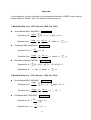
1. Model M0 (Otis et al., 1978; Darroch, 1958; Yip, 1991):
z
Unconditional MLE: M0(UMLE)
Back to Table2
∂ log L Mt +1
Equation for N:
= ∑ (N − j + 1) −1 + t log(1 − p ) = 0 ,
∂N
j =1
Equation for p:
z
∂ log L n • Nt − n •
t
= 0, where n • = ∑ j =1 n j .
=
−
∂p
p
1− p
Conditional MLE: M0(CMLE)
Equation for N: 1 −
Equation for p:
z
Back to Table2
M t +1
= (1 − p )t ,
N
∂ log L n • Nt − n •
t
=
−
= 0, where n • = ∑ j =1 n j .
1− p
∂p
p
Estimating Equation: M0(EE)
Equation for N :
Back to Table2
t
∑ [(N − M
j =1
Equation for p :
j
)(1 − p )] −1 [u j − (N − M j )p] = 0 ,
n• − Np = 0, where n • = ∑ j =1 n j .
t
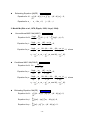
2. Model Mt (Otis et al., 1978; Darroch, 1958; Yip, 1991):
z
Unconditional MLE: Mt(UMLE)
Equation for N:
Equation for ej:
z
∂ log L
=
∂N
Back to Table2
M t +1
∑ (N − j + 1)
−1
j =1
t
+ ∑ log(1 − e j ) = 0,
j =1
∂ log L n j N − n j
=
−
= 0, j = 1, 2,..., t .
∂ ej
e j 1− e j
Conditional MLE: Mt(CMLE)
Back to Table2
t
M t +1
= ∏ (1 − e j ),
N
j =1
nj
Equation for ej: e j = , j = 1, 2,K, t .
N
Equation for N: 1 −
- 27 -
z
Estimating Equation: Mt(EE)
Back to Table2
t
∑ [(N − M
Equation for N :
j =1
Equation for e j :
j
)(1 − e j )] −1 [u j − (N − M j )e j ] = 0 ,
n j − Ne j = 0,
j = 1, 2,..., t .
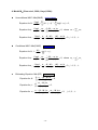
3. Model Mb (Otis et al., 1978; Zippin, 1956; Lloyd, 1994):
z
Unconditional MLE: Mb(UMLE)
Equation for N:
Back to Table2
t
∂ log L Mt +1
= ∑ (N − j + 1) −1 + ∑ log(1 − p ) = 0 ,
∂N
j =1
j =1
Equation for φ :
∂ log L m• (M • − m• ) p
= 0,
=
−
∂φ
φ
1− φ p
Equation for p:
∂ log L n • Nt − M j +1 − M • (M • − m• ) φ
=
−
−
= 0, where
1− p
1− φ p
∂p
p
n • = ∑ j =1 n j , m• = ∑ j =1 m j and M • = ∑ j =1 M j .
t
z
t
t
Conditional MLE: Mb(CMLE) Back to Table2
M t +1
Equation for N: N =
,
1 − (1 − p )t
Equation for φ :
∂ log L m• (M • − m• ) p
= 0,
=
−
∂φ
φ
1− φ p
Equation for p:
∂ log L n • Nt − M j +1 − M • (M • − m• ) φ
=
−
−
= 0, where
∂p
p
1− p
1− φ p
n • = ∑ j =1 n j , m• = ∑ j =1 m j and M • = ∑ j =1 M j .
t
z
Estimating Equation: Mb(EE)
Equation for N :
∑ [(N − M
j
)(1 − p )] −1 [u j − (N − M j )p] = 0,
t
∑ [φ p(1 − φ p)]
−1
j =1
Equation for p :
t
∑ [ p(1 − p)]
j =1
t
Back to Table2
t
j =1
Equation for φ :
t
−1
[m j − M j φ p] = 0 ,
[u j − (N − M j )p] = 0 .
- 28 -
4. Model Mtb (Chao et al., 2000; Lloyd, 1994):
z
Unconditional MLE: Mtb(UMLE)
Equation for N:
Equation for φ :
Equation for e j :
z
t
∂ log L Mt +1
= ∑ (N − j + 1) −1 + ∑ log(1 − e j ) = 0 ,
∂N
j =1
j =1
∂ log L m• t (M j − m j ) e j
t
=
−∑
= 0, where m• = ∑ j =1 m j .
∂φ
φ
1− φ e j
j =2
∂ log L n j N − M j +1 (M j − m j ) φ
=
−
−
= 0, j = 1, 2,K, t .
ej
1− e j
1− φ e j
∂e j
Conditional MLE: Mtb(CMLE)
Equation for N: 1 −
Equation for φ :
Equation for e j :
z
Back to Table2
Back to Table2
t
M t +1
= ∏ (1 − e j ) ,
N
j =1
∂ log L m• t (M j − m j ) e j
t
=
−∑
= 0, where m• = ∑ j =1 m j .
1− φ e j
∂φ
φ
j =2
∂ log L n j N − M j +1 (M j − m j ) φ
=
−
−
= 0, j = 1, 2,K, t .
ej
1− e j
1− φ e j
∂e j
Estimating Equation: Mtb (EE)
Equation for N :
Equation for φ :
Equation for e j :
Back to Table2
t
u j − (N − M j ) e j
j =1
(N − M j )(1 − e j )
∑
t
mj − M jφ ej
j =1
(1 − φ e j )
∑
u j − (N − M j ) e j
(1 − e j )
- 29 -
=0,
= 0,
+
mj − M jφ ej
(1 − φ e j )
= 0,
j = 1, 2,K, t .
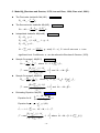
5. Model Mh (Burnham and Overton, 1978; Lee and Chao, 1994; Chao et al., 2001):
z
The First-order Jackknife: Mh (JK1)
z
t −1
Nˆ J 1 = M t +1 + (
)f1t .
t
The Second-order Jackknife: Mh(JK2)
Back to Table2
Back to Table2
2t − 3
(t - 2) 2
Nˆ J 2 = M t +1 + (
)f1t f 2t .
t
t (t − 1)
z
Interpolated Jackknife: Mh(IntJK)
Back to Table2
Nˆ J = Nˆ J 1, g = 1 ,
Nˆ J = cNˆ J , g + (1 − c )Nˆ J , g −1, 1 < g < 5 ,
Nˆ J = Nˆ J 5 , g ≥ 5 ,
t
Nˆ Jl = ∑ j =1 alj f jt , c =
( 0.05 −Pg −1 )
( Pg −Pg −1 )
, g = min{ l : Pl > α } , Pl is the P-value and α is the
significant level. Coefficients alj can be referred to Burnham & Overton (1978).
z
Sample Coverage1: Mh(SC1) Back to Table2
M
f
t
Nˆ sc1 = t +1 + 1t γˆ12 , where Cˆ 1 = 1 − f1t ∑ j =1 jf jt ,
ˆ
ˆ
C
C
1
1
⎧ Nˆ 0, 1t ∑t j ( j − 1)f jt
⎫
⎪
⎪
j =2
−
γˆ = max ⎨
1
,
0
⎬ and Nˆ 0, 1 = M t +1 Cˆ 1 .
t
2
−
t
jf
(
1
)(
)
⎪⎩
⎪⎭
∑ j =1 jt
Sample Coverage2: Mh(SC2) Back to Table2
M
f
t
Nˆ SC 2 = t +1 + 1t γˆ 22 , where Cˆ 2 = 1 − [f1t − 2f 2t (t − 1)] ∑ j =1 jf jt ,
Cˆ
Cˆ
2
1
z
2
2
⎧ Nˆ 0, 2 t ∑t j ( j − 1)f jt
⎫
⎪
⎪
j =2
−
γˆ = max ⎨
1
,
0
⎬ and Nˆ 0, 2 = M t +1 Cˆ 2 .
t
2
−
t
jf
(
1
)(
)
⎪⎩
⎪⎭
∑ j =1 jt
Estimating Equation: Mh(EE) Back to Table2
2
2
z
Equation for N :
t
∑
j =1
u j − (N − Mˆ *j ) p
=0,
(1 − Cˆ )
j −1
Equation for p : p = ∑ j =1 n j /(tN ) .
t
j
Cˆ j −1 = 1 − f1 j / ∑k =1 n k , Mˆ *j = M j + f1, j −1 γˆ h2 ,
⎧ Nˆ 0 t ∑t j ( j − 1)f jt
⎫
t
⎪
⎪
j =1
−
γˆ = max ⎨
1
,
0
, where Nˆ 0 = M t +1 /[1 − f1t /( ∑ j =1 jf jt )] .
⎬
t
2
⎪⎩ (t − 1) ( ∑ j =1 jf jt )
⎪⎭
2
h
- 30 -
6. Model Mth (Lee and Chao, 1994; Chao et al., 2001):
z
Sample COverage1: Mth(SC1)
Back to Table2
M
f
Nˆ sc1 = t +1 + 1t γˆ12 , where
Cˆ 1 Cˆ 1
Cˆ 1 = 1 − f1t
∑
t
j =1
jf jt ,
t
⎫
⎧ˆ
N
j ( j − 1)f jt
∑
0
,
1
⎪
⎪
j =2
2
γˆ1 = max ⎨
− 1, 0 ⎬ ,
n j nk
ΣΣ
⎪
⎪
j <k
⎭
⎩
Nˆ 0, 1 = M t +1 Cˆ 1 .
z
Sample Coverage2: Mth(SC2)
Back to Table2
M
f
Nˆ SC 2 = t +1 + 1t γˆ 22 , where
Cˆ 2
Cˆ 2
Cˆ 2 = 1 − [f1t − 2f 2t (t − 1)]
∑
t
j =1
jf jt ,
t
⎧ˆ
⎫
⎪ N 0, 2 ∑ j =2 j ( j − 1)f jt
⎪
− 1, 0 ⎬ ,
γˆ = max ⎨
2 ΣΣ n j n k
⎪
⎪
j <k
⎩
⎭
2
2
Nˆ 0, 2 = M t +1 Cˆ 2 .
z
Estimating Equation: Mth(EE)
Equation for N :
t
∑
j =1
Back to Table2
u j − (N − Mˆ *j )α j
=0,
(1 − Cˆ j −1 )[1 − (1 + γˆth2 )α j ]
Equation for α j : α j = n j / N, j = 1, 2, K, t ,
where α j = p e j , j = 1, 2, K, t ,
Cˆ j −1
t
⎧ˆ
N
j ( j − 1)f jt
∑
0
⎪
j =1
= 1 − u j / n j , Mˆ *j = M j + f1, j −1 γˆ th2 , γˆ th2 = max ⎨
− 1,
(
2
)
n
n
∑
j
k
⎪
j <k
⎩
t
and Nˆ 0 = M t +1 /[1 − f1t /( ∑ j =1 jf jt )] .
- 31 -
⎫
⎪
0⎬,
⎪
⎭
7. Model Mbh (Pollock and Otto, 1983; Lee and Chao, 1994; Chao et al., 2001):
z
Jackknife: Mbh (JK)
Back to Table2
Nˆ JN = M t + t ⋅ u t .
z
Sample Coverage: Mbh (SC)
Nˆ SC =
Back to Table2
M j +1 j ⋅ u j 2
+
γˆ j , where
Cˆ j
Cˆ j
j = max{ k : u k +1 ek +1 < u1 e1 , k = 1,L, t − 1} ,
Cˆ j = 1 − u j +1 u1 ,
⎧⎪ Nˆ 0, j (u1 − u 2 )
⎫⎪
− 1, 0 ⎬ ,
2
u1
⎪⎩
⎪⎭
γˆ 2j = max ⎨
Nˆ 0, j = M j +1 Cˆ j .
z
Estimating Equation: Mbh (EE)
Equation for N :
t
∑
j =1
Equation for φ :
u j − (N − Mˆ *j ) p
=0,
(1 − Cˆ )
j −1
t
∑ (m
j =1
Equation for p :
Back to Table2
j
− Mˆ *j φ p ) = 0 ,
⎧⎪ u j − (N − Mˆ *j ) p
m j − Mˆ *j φ p ⎫⎪
+
⎨
⎬ = 0,
∑
2
2
γ
φ
p
[
1
−
(
1
+
ˆ
)
]
j =1 ⎪ [1 − (1 + γˆ bh ) p ]
⎪⎭
bh
⎩
t
2
Cˆ j −1 = Cˆ j −1 (φ ) = 1 − u j /(u j + m j / φ ) , Mˆ *j = M j + ( j − 1) u j −1 γˆ bh
,
γˆ
2
bh
⎧ Nˆ h t
⎪
2
= γˆ bh (φ ) = max ⎨
⎪⎩
∑
t
j =1
[ j ( j − 1)f jt + 2(φ − 1)( j − 1)f jt ]
(t − 1) [∑ j =1(m j + φ u j )] 2
t
Nˆ h is a simple estimator valid under model Mh, that is
t
Nˆ h = [M t +1 + f1t γˆ h2 ] /[1 − f1t /( ∑ j =1 jf jt )] .
- 32 -
⎫
⎪
− 1, 0⎬, where
⎪⎭
8. Model Mtbh (Chao et al., 2001):
z
Estimating Equation: Mtbh(EE)
Equation for N :
t
∑
j =1
Equation for φ :
t
∑
j =1
αˆ j = αˆ j (φ , N ) =
Back to Table2
Mˆ *j (φ u j + m j ) − Nm j
= 0,
2
(1 − Cˆ j −1 )[1 + (φ − 1)Cˆ j −1 − φ (1 + γˆtbh
) αˆ j ]
Mˆ *j (φ u j + m j ) − Nm j
= 0.
2
[1 + (φ − 1)Cˆ j −1 − φ (1 + γˆtbh
)αˆ j ]
2
A j − [ A 2j − 4Nφn j (1 + γˆtbh
)]1/ 2
2
2Nφ (1 + γˆ tbh
)
, where
2
2
A j = A j (φ , N ) = N + φn j (1 + γˆ tbh
) + (φ − 1)[NCˆ j −1 − (1 + γˆ tbh
)m j ].
j −1
2
Cˆ j −1 = Cˆ j −1 (φ ) = 1 − u j /(u j + m j / φ ) , Mˆ *j = M j + [∑k =1 ρˆ k , j −1 ] u j −1 γˆtbh
,
γˆ
2
tbh
⎧ Nˆ bh ∑t [ j ( j − 1)f jt + 2(φ − 1)( j − 1)f jt ]
⎫
⎪
⎪
j =1
= γˆ (φ ) = max ⎨ t
1
,
0
−
⎬, where
t
2
2
[
(
)]
(
)
+
−
+
m
φ
u
m
φ
u
⎪⎩ ∑ j =1 j
⎪⎭
∑ j =1 j
j
j
2
tbh
Nˆ bh is a simple estimator valid under model Mbh. Here, ρ k , j −1 = e k / e j −1
denotes the unknown relative time effect of sample k. A convenient estimator of
ρ k , j −1 = e k / e j −1 is a function of φ and can be presented as
ρˆ k , j −1 = ρˆ k , j −1(φ ) = (u k + mk / φ ) /(u j −1 + m j −1 / φ ) .
- 33 -