Download esys-Escript User's Guide: Solving Partial Differential Equations with

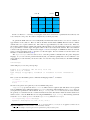
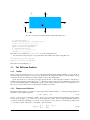
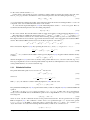
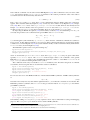
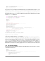
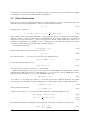
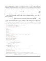
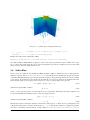
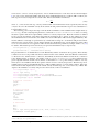
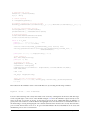
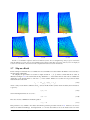
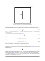
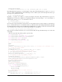
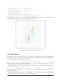
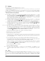
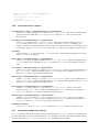
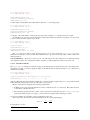
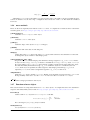
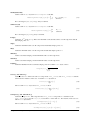
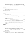
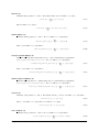
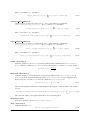
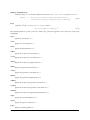
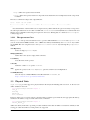
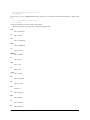
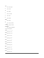
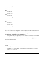
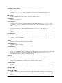
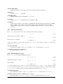
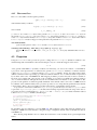
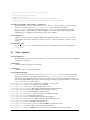
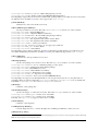
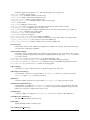
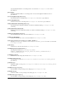
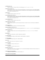
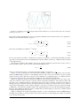
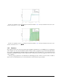
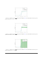
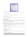
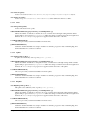
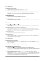
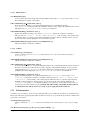
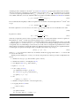
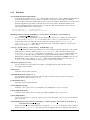
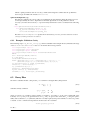
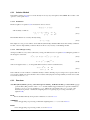
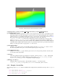
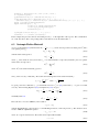
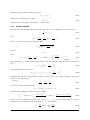
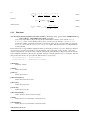
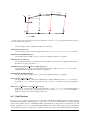
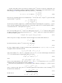
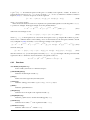
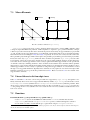
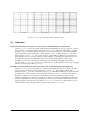
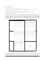
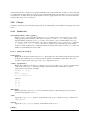
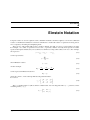
A fault t in the fault system is represented by a starting point V t0 and series of directions, called strikes, and
the lengths (lti ). The strike of segment i is defined by the angle σ ti between the x0 -axis and the direction of the
fault, see Figure 6.2. The length and strike defines the polyline (V ti ) of the fault by


cos(σ ti )
V ti = V t(i−1) + lti · S ti with S ti =  sin(σ ti ) 
(6.68)
0
In the 3D case each fault segment i has an additional dip θti and at each vertex i a depth δ ti is given. The fault
segment normal nti is given by


−sin(θti ) · S1ti
nti =  sin(θti ) · S0ti 
(6.69)
cos(θti )
At each vertex we define a depth vector dti defined as the intersect of the fault planes of segment (i − 1) and i
where for the first segment and last segment the vector orthogonal to strike vector S ti and the segment normal nti
is used. The direction d˜ti of the depth vector is given as
d˜ti = nti × nt(i−1)
(6.70)
If d˜ti is zero the strike vectors Lt(i−1) and Lti are collinear and we can set d˜ti = lti × nti . If the two fault segments
are almost orthogonal d˜ti is pointing in the direction of Lt(i−1) and Lti . In this case no depth can be defined. So
we will reject a fault system if
min(kd˜ti × Lt(i−1) k, kd˜ti × Lti k) ≤ 0.1 · kd˜ti |
(6.71)
which corresponds to an angle of less than 10o between the depth vector and the strike. We then set
dti = δ ti ·
d˜ti
kd˜ti k
(6.72)
We can then define the polyline (v ti ) for the bottom of the fault as
v ti = V ti + dti
(6.73)
In order to simplify working on a fault t in a fault system a parameterization P t : (w0 , w1 ) → (x0 , x1 , x2 ) over a
rectangular domain is introduced such that
t
t
0 ≤ w0 ≤ w0max
and − w1max
≤ w1 ≤ 0
(6.74)
t
t
t
with positive numbers w0max
and w1max
. Typically one chooses w0max
to be the unrolled length of the fault and
t
w1max to be the mean value of segment depth. Moreover we have
P t (W ti ) = V ti and P t (wti ) = v ti
(6.75)
t
W ti = (Ωti , 0) and wti = (Ωti , −w1max
)
(6.76)
where
t
and Ωti is the unrolled distance of W ti from W t0 , i.e. lti = Ωt(i+1) − Ωti . In the 2D case w1max
is set to zero
and therefore the second component is dropped, see Figure 6.2.
In the 2D case the parameterization P t is constructed as follows: The line connecting V t(i−1) and V ti is given
by
x = V ti + s · (V t(i+1) − V ti )
(6.77)
where s is between 0 and 1. The point x is on i-th fault segment if and only if such an s exists. Assuming x is on
the fault it can be calculated as
(x − V ti )t · (V t(i+1) − V ti )
(6.78)
s=
kV t(i+1) − V ti k2
We then can set
w0 = Ωti + s · (Ωti − Ωt(i−1) )
Chapter 6. Models
(6.79)
115