Download Operating Instructions for the online tool “rainwater harvesting and

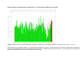
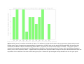
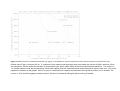
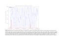
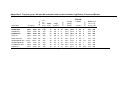
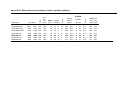
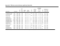
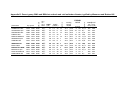
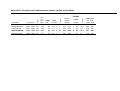
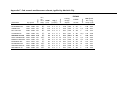
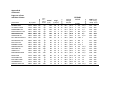
Operating Instructions for the online tool “rainwater harvesting and demand simulation” - a.k.a. http://GetTanked.org
Accessed from either instance http://rainwater.vpac.org or http://rainwater.vulabs.net
Author Eric Laurentius Peterson ¹ ² *
¹ Adjunct Professor, Institute for Sustainability and Innovation, Victoria University, Melbourne, Australia
² Adjunct Senior Fellow, School of Civil Engineering, University of Queensland, St Lucia, Australia
Contact email [email protected]
These instructions are in support of the manuscript “Transcontinental assessment of secure rainwater harvesting systems across Australia”,
Submitted to Resources, Conservation & Recycling 29th December 2014, returned 20th March with comments, resubmitted 20th April 2015.
The author hereby documents recommended use of the online tool “rainwater harvesting and demand simulation” linked to from the website
URL http://gettanked.org/, which serves only the Australian continent and Tasmania. This tool dynamically calculates the irrigation and
evaporative cooling demands in addition to any particular per diem allocation of potable water. The analysis may be either from a finite storage
tank of specified capacity, or drawn from water mains.
The nominal daily potable water demand of 144 litres per person per diem needs to be critically questioned by any user, and as a result of
experience of the Millennium Drought it may be workable to reduce demand to 100 litres per person per diem, cover swimming pools,
implement recycling of grey water to supplement irrigation, and to provide shade cloth cover over gardens during heat waves. In surviving
drought it is reasonable to maintain the amenity of shade trees and a small garden as well as providing evaporative cooling indoors. If demand
can be rationed and appropriately recycled, then secure rainwater harvesting system may be designed to serve in many parts of the Australian
continent if sufficient catchment and capacity are provided, or if occasional tanker deliveries are readily available. Tables, sorted by climate
classification are found in Appendices A through H of these instructions to tabulate demand restrictions that have been found to avoid running
dry within the constraints of a nominal 10 m³ capacity storage with 100 m² catchment– defining the sustainable load per diem (SLPD) during a
“worst case” epoch – this is the break-point for absolute security as far as meteorological records can determine since European settlement.
SLPD varies from 86 to 124 L/d among most temperate maritime climate stations, and between 35 and 42 L/d at most desert climate stations.
Appendix Tables A through H also summarize demand for evaporative cooling and irrigation together with the sustainable yield of a rainwater
harvest system at 128 locations throughout Australia.
Indoor and potable water demand should be disaggregated from irrigation, pool evaporation, and evaporative cooling to make use of this tool.
Material and methods
FAO56 irrigation demand (Allen, et al. 1998), and pan evaporation reference the patched point dataset (PPD) data bank, commencing in 1890
for rainfall and 1957 for climate variables (Jeffery, et al. 2001). Daily minimum and maximum temperature and vapour pressure provided by the
PPD, together with atmospheric pressure estimated from altitude are used to model the part-load performance of evaporative coolers if the fullload cooling demand is specified. Daily cooling load is scaled on basis of cooling degree days to the base 24°C as described by Peterson
(2014) with design drybulb at the locality calculated for the specified epoch by the method of Peterson, et al. (2006). Backend computations
and graphics are provided by GNU Octave following an M-file script that is customized in response to the details entered into data forms on the
GetTanked website frontend. The website frontend is comprised of javascripts that were compiled with Google Web Toolkit.
In order to speed up simulations of multiple combinations of rainwater harvesting system parameters it was decided that the GetTanked tool
must first-pass establish a “worst case” quadrennium (4 year epoch).at the case study of interest. The nomination of “worst case” is
determined by searching for the two-consecutive years with respect to the difference between rainfall and Australian synthetic Class A pan
evaporation. GetTanked includes the formative year as well as the succeeding year to nominate a moderated “worst case” epoch.
References
Allen RG, Pereira LS, Raes D, Smith M. 1998. Crop evapotranspiration—guidelines for computing crop water requirements: FAO irrigation and drainage
paper 56. Rome: FAO–Food and Agriculture Organization of the United Nations. http://www.fao.org/docrep/X0490E/X0490E00.htm
Jeffrey, S. J., Carter, J. O., Moodie, K. B., & Beswick, A. R. (2001). Using spatial interpolation to construct a comprehensive archive of Australian climate data.
Environmental Modelling & Software, 16(4), 309-330.
Peterson, E., Williams, N., Gilbert, D., & Bremhorst, K. (2006). New air conditioning design temperatures for Queensland, Australia. AIRAH Equilibrium
February 2006. http://mail.airah.org.au/downloads/2006-02-01.pdf
Peterson, E (2014). Mitigation of the energy-water collision through integrated rooftop solar and water harvesting and use for cooling: A critical review. In:
What conditions must models and methods fulfill on an urban scale to promote sustainability in buildings? Proceedings of the World Sustainable Building
Conference 2014, Barcelona. ISBN 978-84-697-1815-5 http://uq.id.au/e.peterson/GetTanked/Peterson_ref110_Paper89.pdf
Graphical Abstract of Rain Water Harvesting and Demand Simulation (Peterson 2015)
Precipitation, R
Bulk make-up, Mt
Area of roof catchment, A
in-flow, I
Evaporative Cooling, kW
overflow, O
full volume Vf
present storage Vt
Potable demand, Dp
Irrigation demand, Dg
Yield, Y
Area of Irrigation, Ag
Evaporation, De
Total demand, Dt
Mains make-up, Mm
Area of water , Ae
Graphical Abstract: Rainwater harvesting and demand system (RWHS) modelled by the GetTanked tool from the paper “Transcontinental assessment of
secure rainwater harvesting systems across Australia”, Submitted to Resources, Conservation & Recycling 20th April 2015.
The parameters operating behind GetTanked are illustrated in the Graphical Abstract submitted to the journal Resources, Conservation &
Recycling. Besides geographical location, adjustable variables include the potable water demand, Dp, evaporative cooler capacity, kW, the
area of garden irrigation demand, Ag, the area of water feature evaporation, Ae, utilized stormwater catchment area, A and the storage capacity
of the tank, volume Vf when full, measured above the minimum allowed reserve. The geographical location determines the rainfall supply onto
the roof catchment while solar radiation, temperature and humidity determine the FAO 65 evapotranspiration potential (irrigation demand), pan
evaporation, and evaporative cooler water consumption. The level of water, Vt, in the storage tank will generally vary at each timestep (daily) t.
As rainfall data is most generally available on a daily basis, GetTanked is designed to investigate the reliability of supply from rainwater with
deficit periodically avoided by bulk delivery Mt, or by continuous mains make-up Mm. Simulations employ an algorithm where the present
storage in the tank Vt is taken as the previous day’s storage in the tank Vt-1 minus the total daily demand, but not allowed to be negative, nor to
exceed the maximum capacity of the tank. As yield is not explicitly calculated to determine occasional tank overflows, this model uses yieldsbefore-spill (YBS). GetTanked operates with an in-built assumption of 10 litres first flush diversion each day that rainwater harvesting occurs.
The behaviour of supplemental water imports depends if there is a continuous connection to mains for makeup on demand Mm, or if bulk
shipments are hauled in to fill the tank whenever it runs dry.
GetTanked users can toggle the “water consumption” data entry form to evaluate the continuous-mains make-up, or estimate tanker-trucking
orders for premises that are off-grid. Bulk tanker deliveries are the method of makeup employed example output Figures 1 – 5, but mains
connected refilling without storage capacity or catchment informs the seasonal demand profiles of irrigation and evaporative cooling. Bulk
tanker make-up is normal practice in situations of rural and peri-urban development, where home owners need to ensure that they hold water
reserves for fire fighting. There is very little spillage before use as such tanker deliveries tend to be conducted during periods of drought, and so
the YBS model is a reasonable method for the purposes of the present study. In either case, yield from the RWHS (Yt) can be calculated as
the minimum of total daily demand (Dt); or the sum of daily in-flow (I) and the previous day’s storage (Vt-1).
GetTanked utilizes Google Maps interface for users to specify location and the trace the catchment areas A that contribute to the RWHS. The
nominated storage tank capacity Vf should be considered by the user by reference to manufacturer’s specification to neglect sludge collection
at the bottom and freeboard in the headspace. For example, a 2.2 m internal diameter tank would need to exceed 2.63 m height to achieve 10
kL capacity Vf, and higher to ensure this represents the active-capacity above any required low-level reserve.
The GetTanked Google Maps interface also allows users to trace the area of evapotranspiration Ag and evaporation demand Ae, or explicitly
specify these areas. GetTanked users may vary the portion of the rooftop rainfall (R × A) entering the inflow of the tank by adjusting the
impermeability of the catchment (nominally 0.95). Similarly the user may vary the FAO56 irrigation demand (FAO56 – R) × Ag by specifying a
screening factor (nominally 0.0). Finally the user may vary water feature (i.e. swimming pool or open-air reservoir) evaporation by specifying a
cover factor (nominally 0.0).
Rainwater harvesting and demand simulation data forms
The rainwater harvesting and demand simulation tool URL http://GetTanked.org has been forwarding to a server at premises of the Victorian
Partnership for Advanced Computing (VPAC), 110 Victoria Street, Melbourne, Australia, but may be redirected elsewhere. In any instance the
website, “Rain Water Harvesting and Demand Simulation”, presents a series of data forms for users to specify rainwater catchment, water
usage and tank storage capacity to simulate the reliability of supply from rainwater, and to identify supplements that may be required.
GetTanked estimates the 'failure rate', being the percentage of imports either made-up from water mains or by tanker truck deliveries. The left
hand pane of GetTanked has a green arrow that notes the user’s progress working through seven data-entry forms between Welcome and
Submit, with “< Prev” and “Next >” to forward and back as much as desired until selecting ‘Submit’ on the last form, with a wait of up to two
minutes for results. Users can revise successive simulations with the “< Prev” and “Next >” toggles, and then submit again before copying
resulting graphics (Figures 1 through 5) for pasting into a report.
1. Location is the first data entry form (after the Welcome notice). Select location by either typing in an address or clicking in the Google Maps
window. This is the only input for which there is no default, and so we illustrate VPAC’s street address “110 Victoria Street, Melbourne” or
geographical coordinates “-37.8066 , 144.9635”. Beware GetTanked runs for any point on earth, using the nearest Australian dataset.
2. Analysis Period is the second data entry form. “Worst Case” or “Manual” specification will be confirmed in Figure 1 in red against the
background 121 years of PPD. In the current study the default “Worst Case” option is always accepted, simply advancing “Next >”.
3. Water consumption specifies either “Total Consumption” or “Consumption based on household population”. The latter is the default, with
2 persons dwelling in the home, with 155 L “Daily water consumption per person”. This default is equivalent to entering 310 L/day “Total
daily consumption” under the alternative tab. Enter 0 if rainwater harvesting system does NOT serve POTABLE needs, and advance to
further data forms to detail modelling of demand for irrigation, evaporative-cooling, and evaporation from swimming pools and water
features. Accept default of 155 L per capita per diem, advancing “Next >”.
4. Rain water collection and storage is the fourth data entry form. Users may specify if mains water is available, but the default setting
(“No”) assumes that a water tanker is despatched to fill the tank if it runs dry. Demand without reference to supply will be profiled if mains
water is declared to be available while also zeroing both tank size and roof size. This form allows adjustment of nominal default 10,000 L
capacity, nominal 100 m² catchment and the rather optimistic suggestion of 95% run-off coefficient (1-permeabilitycatchment). Note that
“capacity” is intended to represent only the active-capacity of a covered storage reservoir, excluding any required reserve. Google imagery
is provided to measure catchment area by tracing polygons over any number of discernible impervious surfaces judged to be useful.
5. Outdoor water use is covered by two data- entry forms, each provided with a Google imagery view of the locality of interest so that the
user can trace polygons over the areas of garden irrigation and water body evaporation that demand water from the rainwater harvesting
tank. Manual data entry of the square meters of irrigated garden and pool area are also provided, with default at zero. If an area is entered
and traced then the default portion covered is zero, which can be adjusted as high as 1 to indicate the area could somehow be absolutely
protected from evaporation or evapotranspiration. Zero cover is assumed throughout the present example. In the present discussion
accept all defaults, with zero area of both garden irrigation and pool evaporation, and also without evaporative cooling. Thereby only a
constant demand for potable water is simulated. Evaporative cooling has been included on the “outdoor water use” form because the
process depends on forced convection of outdoor air through the building to displace heat with air approaching the wetbulb temperature of
the outdoor air conditions. The evaporative cooling model integrated into GetTanked was described by Peterson (2014), and depends on
the user declaring the total cooling capacity of installed evaporative coolers. Direct evaporative cooling does not work when wetbulb
temperatures are above the desired indoor temperature of 24°C, and therefor at such times vapour-compression air-conditioning systems
could be desired. GetTanked models the consumption of water effectively evaporated, and so splits the demand peaks of spring and
autumn – indicating evaporative cooling is often ineffective during summer in such locations.
6. Outdoor water use continued The second outdoor water use form is concerned with evaporation from uncovered water features such as
swimming pools or any storage reservoir exposed to pan-like evaporation losses. For the initial illustration of methodology without nonpotable demands accept all defaults on both “Outdoor Water Use” forms, simply stepping forwards “Next >” and then “Next >”
7. User contact details Ambit users may directly click the final “Next >” to skip past the 7th form unless willing to collaborate with the author in
a case study or to offer critique. Use of this form is necessary if the user wishes to request a copy of the M-file script that runs on the server,
but it is also best to email the author as a prompt because the user register is rarely used and so routine monitoring has not been justified.
The forgoing data-forms are analysed by selecting the ”Submit” button to pass parameters to a computer server with results to be displayed
once the simulation has completed. It usually takes just one minute for a four-year analysis (default) if no other users happen to submit a job at
the same moment. Analysis with evaporative cooling may take two minutes. Figures 1, 2, 3, 4, 5, and “Summary” appear on completion.
Select the desired figure tab and then click within the figure to maximize the display and then click again to review other figures or to review
data entry forms from “< Prev”. Users may copy figures using right mouse-key “Save picture as”, or “copy” and then paste into a document
together with Summary text.
Repeatedly skipping through all forms (“Next>”) without amending anything other than the address ignores the buildings that may be discerned
in Google imagery. The default 10,000 L active-volume of the tank is fed by 100 m ² catchment with 95% runoff coefficient (5% permeability)
supplying a fixed 310 L daily demand during the particular location’s “worst case” quadrennium (4 years period covering an El Niño event).
Scripting GetTanked Rain Water Harvesting and Demand Simulation
While all of the results presented in these operating instructions were obtained via the GetTanked website interface, interested researchers and
professionals could run simulations offline if they install MatLAB or Octave and obtain PPD data from Queensland Science Delivery Division of
the Department of Science, Information Technology, Innovation and the Arts (DSITIA) https://www.longpaddock.qld.gov.au/silo/ppd/format.php
specified to be in the “Standard including FAO56 Reference Evapotranspiration (ETo)” format and copy into a data folder with the station
identification number appended by “.txt” suffix.
Each run of the on-line GetTanked tool is custom written in the GNU Octave M-file script that can be obtained by completing the user contact
details before submitting a simulation to the GetTanked server http://rainwater.vpac.org. It is then recommended to email the author because
user comments are rarely completed, and so the feedback register is seldom monitored. The author can reply with the user’s simulation script,
but it must be renamed something short ending with the M-file suffix “.m” and amended wherein the UNIXpath2SILO and/or DOSpath2SILO
variables match the local users’ “data” repository of PPD files and an ASCII file named “station_ID_altitude.csv” containing four columns of
comma separated station identifier (sorted by ascending BoM number), latitude (°), longitude (°), elevation (m) for each station of the “data”
subfolder:
station1, latitude1, longitude1, elevation1
station2, latitude2, longitude2, elevation2
…
stationn, latituden, longituden, elevationn
In the example simulation at the premises of VPAC the station_ID_altitude.csv should contain at least one line “86071,-37.8075,144.97,31.2”
while the folder “data” must contain a PPD file named “86071.txt” if not all of the 4759 stations that can be subscribed to.
Furthermore the header of PPD files are six lines longer than those that were integrated into the on-line GetTanked tool and so the M-file script
must be amended such that lines defining “unix_command1” and “dos_command1” should be replaced as follows:
unix_command1=['sed ''1,54d'' ',filename,' > ',filelessheader];
dos_command1=['more +54 ',filename,' > ',filelessheader];
Default output for example address in Melbourne: 110 Victoria Street, Melbourne, Australia
Figure 1: Default output from website GetTanked.org “Figure 1” for Melbourne. The difference between evaporation and rainfall over 121 years.
Default output for the example address “110 Victoria Street, Melbourne”, Figure 1, illustrates that the “worst case” quadrennium was taken at
the end of the available time series, immediately before the return of La Niña wet seasons 2010 and 2011. The vertical axis is the difference
between Australian synthetic Class A pan evaporation and rainfall.
Figure 2: Default output from website GetTanked.org “Figure 2” for Melbourne. Average monthly water make-up requirement during simulation epoch.
Default output Figure 2 presents the seasonal pattern of imports into a 10,000 L tank over the epoch 2006 through 2009, and confirms that
simulations are based on Bureau of Meteorology station 86071, lying about one km east of the location of interest. During the 4 years of
simulation the average monthly demand for trucking imports is presented. Note that the months of February, April, and October averaged a
delivery of one 10 kL shipment of water. It appears that no shipments were required in March or April of the epoch, and that deliveries were not
required all of four instances of the other months during the epoch. Beware this plot averaged monthly demand over the four year epoch.
Figure 3: Default output from website GetTanked.org “Figure 3” for Melbourne. Import requirement varies with tank capacity and catchment area.
Default output Figure 3 presents 56 (8 × 7) variations of tank capacity and catchment area surrounding the nominal 10,000 L tank and 100 m²
roof catchment, with the statement that 64% of demand during the epoch (2006-2009) would have required tanker deliveries. The contour of
1% shortfall makes it clear that a quadrupling of both tank capacity and roof catchment would reduce demand for imports near zero. Due to the
logarithmic character of this graphic, there is no point in combinations of capacity and catchment far beyond the contour of 1% shortfall. The
contour of 10% shortfall suggests possibly economic solutions if occasional refilling by tanker trucking is feasible.
Figure 4: Default output from GetTanked.org “Figure 4” for Melbourne. Timeline of tank capacity and overflows for nominal capacity and catchment area
Default output Figure 4 provides a daily time-series of the tank capacity and overflow events during the epoch (2006-2009). Rainwater overflow
events indicate that more tank capacity would be useful to avoid later demand for refilling. Tanker truck deliveries are implied when the capacity
curve runs vertically from near zero, up to near the nominated capacity level (10,000 L) without the coincidence of overflow. There are 29
tanker filling events observed on this plot that can be confirmed by reference to the average monthly demand for imports presented in Figure 2.
Figure 5: Default output from website GetTanked.org “Figure 5” for Melbourne. Import requirement varies with recycling of grey water to supplement
outdoor irrigation. Without specification of irrigated area the only advice of this figure is to manage the daily demand for potable water indoors.
Default output Figure 5 is similar to Figure 3 by stating the nominal RWHS would have required tanker truck deliveries to make-up 64% of
demand, but in the case of Figure 5 the nominal among 60 combination (10 × 6) variations of demand and increasing rates of recycling greywater after use as indoor potable water to meet irrigation needs outdoors, and by varying the demand for indoor potable water. Truncated text
in the upper left corner is intended to label “Grey water irrigation AND potable water conservation” Truncated text in the lower left corner is
intended to label “Use less potable water”. Unfortunately the contour labels of 1% shortfall and 10% shortfall are overwritten.
Workflow recommendations
A number of useful outputs require comparative re-simulation as they are not available first-pass through the rain water harvesting and
demand simulation tool that is found from the link at URL GetTanked.org
For example Sustainable Litres Per Diem (SLPD*) in the example of default output for Melbourne, Figure 5 resolves that the demand should be
managed somewhere above 78 and below 155 litres per day during the “worst case” drought epoch. The particular breakpoint was later found
to be 104 L/d at the example address. The breakpoint is here-to-for referred to as SLPD* where the asterisk denotes that 10,000 L storage and
100 m² catchment defaults apply. The Appendix tables present the SLPD* found at 128 locations around Australia, but at any other location
the user is offered the following workflows to determine their locally relevant values of key indicators of RWHS performance.
a. Sustainable Load Per Diem
The sustainable demand per diem was determined by repeatedly stepping back and forth between the water consumption and submit forms,
with a delay of one minute per iteration. Each time inspect Figure 5 and note percentage filling required as well as the demand level closest to
the curve of 1% shortfall. Iteration steps are manually continued until they confine the breakpoint of absolute reliability, between two steps
separated by one litre per diem. The result is the sustainable load per diem (SLPD*) at the location of interest, where the asterisk indicates the
default storage capacity of 10,000 litres and catchment area of 100 m². For example SLPD* is found to be 104 L/d at the example address of
110 Victoria Street, Melbourne. In many locations SLPD* is less than 100 L/d, in which case the percentage shortage over the drought epoch
(short) is tabulated in Appendices A-H so that tanker supplements can be arranged if demand remains at constant level of 100 L/d.
b. Irrigation (Irrig †)
Irrigation demand of any particular situation is obtained by stepping back (“<Prev”) three data entry forms to specify irrigated garden area, then
back (“<Prev”) another data entry form to toggle YES with regard to mains water supply and to zero both tank size and roof size, and then back
(“<Prev”) one more data entry form to zero potable consumption. Finally forwarding (“Next>”) five data entry forms and reactivating the
“Submit” button produces a revised set of Figures 1 through 5. Specifying 10 m² irrigation in the otherwise default output for 110 Victoria Street,
Melbourne yield revised Summary Results text: “Assuming an irrigated garden and/or lawn area of 10 square meters.” and “Lawn and garden
demand was 100%. The total average demand was 29 L/d, with maximum 92 L/d.”
Summary Results text also includes the average and maximum daily demand that would be met with a limitless water mains service – without
the nominal rainwater harvesting system. Divide irrigation demand by the irrigated area and report as Irrig †, 2.9:9.2 L/d/m² (av:max).
c. Greywater irrigation (recycling indoor potable water after first use)
It is reasoned that a per diem ration of 100 litres of potable water may be manageable while non potable demands are also supplied as needed.
This suggests two persons dwelling under 100 m² adapting lifestyle to severe drought restrictions, or one person living more lavishly therein.
Having completed irrigation-only demand results, step back (“<Prev”) five forms to toggle “Total Consumption” and specify the total daily
consumption at 100 litres per day (per diem). Then step forward (“Next>”) one form to toggle “No” mains connection and restore the nominal
RWHS (roof size 100 m² feeding 10,000 L tank size). Finally step forward to reactivate the “Submit” button and wait a minute. In the case of
Melbourne the nominal RWHS serving 10 m² of garden, then reliability is ensured if 64% of potable demand is recycled for irrigation –
otherwise tanker deliveries are required to make-up 21% of demand during the “worst case” epoch, denoted in the revised output “Figure 5”.
d. Evaporative cooling demand per diem per kW capacity (ECDkW)
Back step and zero all dataforms, except to specify the house equipped with an evaporative cooler having a nominal capacity of 3.5 kW (1 ton
of avoided air-conditioning), and step forward to reactivate the “Submit” button and wait two minutes. In this example GetTanked has simulated
a 1 ton (3.5 kW) evaporative cooling system’s performance in Melbourne, where Summary Results report an average 18 L./d demand with
peak 166 L/d. Revised “Figure 2” shows the peak occurs in March and a secondary peak in January. In the case of Melbourne the result
range 5 to 47 L/d/kW and are listed in the results of this study as the evaporative cooling demand per kW capacity, 5:47 ECDkW L/d/kW
(av:max).
e. Total demand for potable water, irrigation, and evaporative cooling (TPIE ‡)
Total demand including 100 L/d potable as well as irrigating 10 m² and 1 ton evaporative cooling is found to average 147 L/d with a peak of
309 L/d in January. Coincidentally, the peak is near Melbourne Water’s drought management “Target 155” for two persons. In the example of
Melbourne, one reliable solution to the problem of ensuring 100 L/d potable supply plus irrigation of 10 m² garden and 1 ton (3.5 kW)
evaporative cooling is to increase storage to 14,000 litres and catchment to 141 m², while providing grey water recycling or provide imports as
illustrated in revised output “Figure 5”.
Acknowledgements
GetTanked was made possible by Victoria University of Technology, which joined the Victorian Partnership for Advanced Computing (VPAC),
to provide logistical support to develop innovative interactive tools. VPAC provided the GetTanked website to read my program script with
open source Octave. Lachlan Hurst developed the Google Maps mashup “front end” alpha version, with final version of the website developed
by Daniel Micevski. Resources, Conservation & Recycling peer-reviewers suggested these operating instructions be freely posted on-line.
Appendix A: Tropical group, Am and Aw monsoon and savanna climates, typified by Cairns and Bowen
pk. mo.
pk. mo.
climate
ECDkW
Cooling
TPIE ǂ total
L/d/kW
SLPD*
Irrig †
Design
Pot. +Irrig
placename
dry epoch
short (L/d)
(L/d/m²)
db/wb
+Evap
(L/d)
av:max
COOKTOWN QLD
2002 2005 Aw
14%
87
3.6 :8 10
35.5 /26.6
8 :49 8
163 :309
CAIRNS QLD
2002 2005 Am 14%
71 3.5 :8 10
34.0 /24.9
9 :55 8
168 :329
DARWIN NT
1978 1981 Aw
27%
63
3.8 :7 9
35.4 /25.8
4 :25 7
153 :248
BOWEN QLD
2001 2004 Aw 41%
51 4.0 :7 11
33.8 /26.7 13 :67 8
187 :372
44%
51
3.6 :6 10
33.5 /26.1
5 :23 8
151 :233
GOVE NT
1951 1954 Aw
PORT KEATS NT
1991 1994 Aw
41%
47
4.2 :8 10
38.1 /27.4
6 :36 7
163 :273
NORMANTON QLD 1970* 1973* Aw
41%
46
5.0 :9 10
39.1 /23.9
8 :38 7,11 176 :278
GEORGETOWN QL
1969 1972 Aw
41%
46
5.0 :9 10
39.9 /23.5 10 :47 7
185 :309
TOWNSVILLE QLD
1993 1996 Aw
34%
44
4.1 :9 1,10 35.0 /24.0 12 :66 7
184 :369
TINDAL NT
1961 1964 Aw
34%
43
4.7 :8 10
40.1 /26.3
9 :43 6,10 179 :295
* Normanton’s epoch 1970-‘73 caused a failure of evaporative cooling calculations, so years 2006-2009 used for ECDkW and TPIE results.
100m²
10kL
100L/d
Appendix B: BSk cold semi-arid (steppe) climate, typified by Mildura
pk. mo.
pk. mo.
climate
ECDkW
Cooling
TPIE ‡ total
L/d/kW
SLPD*
Irrig †
Design
Pot. +Irrig
short (L/d)
(L/d/m²)
db/wb
+Evap
(L/d)
placename
dry epoch
av:max
KYANCUTTA SA
2006 2009 BSk 34%
65 3.7 :10 1
43.6 /22.4
9 :45 10,12
170 :293
NORSEMAN WA
1971* 1974* BSk 34%
62 3.7 :9 12 40.7 /22.7
9 :53 12,3
169 :318
LAKE GRACE WA
1972 1975 BSk 27%
62 3.4 :9 12 39.3 /21.1
8 :51 3,12
163 :323
SOUTHERN CROSS
1976 1979 BSk 41%
59 4.0 :9 1
40.8 /20.1
8 :50 11,4
168 :310
WAILLTON VIC
1981 1984 BSk 21%
56 2.9 :9 12 40.5 /21.6
7 :52 12,2
155 :327
MILDURA VIC
2006 2009 BSk 55%
51 3.9 :9 1
41.9 /21.3
8 :43 12
166 :293
SWAN HILL VIC
1981 1984 BSk 27%
49 3.5 :9 1
41.3 /21.6
8 :40 12,3
162 :290
RENMARK WA
2002 2005 BSk 48%
45 3.8 :10 1
41.1 /20.7 10 :51 3,12
172 :306
* Norseman’s dry epoch 1971-1974 caused a failure of evaporative cooling calculations, so year 2006-2009 used for ECDkW and TPIE results.
100m²
10kL
100L/d
Appendix C: BSh hot semi-arid climate, typified by Charleville
pk. mo.
pk. mo.
climate
ECDkW
Cooling
TPIE ‡ total
L/d/kW
Design
Pot. +Irrig
SLPD*
Irrig †
short (L/d)
db/wb
+Evap
(L/d)
placename
dry epoch
(L/d/m²)
av:max
TENNANT CREEK N
1985 1988 BSh 48%
76 5.6 :9
11
41.5 /21.4 10 :33 1
193 :287
CUNNAMULLA QLD 2005 2008 BSh 34%
66 4.8 :9
1,10 43.1 /22.2
8 :40 9,4
127 :233
DALWALLINU WA
1976 1979 BSh 27%
63 4.1 :10 1
41.7 /21.3
8 :39 11,4
168 :288
QUILPIE QLD
2005 2008 BSh 34%
60 5.1 :9
1,10 43.2 /25.2
9 :41 5,9,1 183 :286
COBAR NSW
2005 2008 BSh 41%
57 4.4 :9
1
41.9 /20.5
7 :38 10,4
168 :304
EMERALD QLD
2002 2005 BSh 27%
52 4.6 :9
11
40.1 /24.7 10 :50 8,5
182 :313
KUNUNURRA WA
1985 1988 BSh 41%
51 5.4 :9
10
42.5 /27.6
7 :25 7,10
179 :269
WYNDHAM WA
1989* 1992* BSh 34%
51 5.6 :9
10
42.1 /27.4
6 :29 7,10
173 :280
CHARLEVILLE QLD
1991 1994 BSh 41%
50 4.7 :9
1
39.8 /21.4 11 :55 9,5
186 :341
KALGOORLIE WA
1976 1979 BSh 55%
45 4.2 :9
1
41.0 /20.4
8 :45 10,4
169 :295
WINTON QLD
1982 1985 BSh 55%
45 5.3 :9
12
42.6 /23.1 10 :49 8,5,1 189 :311
MOUNT ISA QLD
1985 1988 BSh 48%
44 5.5 :9
1,10 41.2 /22.5 11 :50 8,1
193 :315
BROOME WA
1992 1995 BSh 51%
38 5.1 :9
11,3 38.6 /22.9
9 :43 7
182 :295
CURTIN WA
1971 1974 BSh 41%
37 5.2 :9
10
41.0 /24.2
8 :37 7,11
179 :272
RICHMOND QLD
2002 2005 BSh 48%
36 5.5 :9
10,3 41.7 /23.4 11 :45 7
195 :299
LONGREACH QLD
2002 2005 BSh 55%
32 5.5 :9
12
42.5 /21.9 11 :48 8,5
195 :310
* Wyndham’s epoch 1989-1992 caused a failure of evaporative cooling calculations, so years 2006-2009 used for ECDkW and TPIE results.
100m²
10kL
100L/d
short
BWh 55%
BWh 48%
BWh 62%
BWh 62%
BWh 55%
BWh 55%
BWh 55%
BWh 62%
BWh 62%
BWk 55%
BWh 55%
BWh 62%
BWh 62%
SLPD*
(L/d)
47
44
42
42
41
38
37
36
35
35
30
27
26
Irrig †
(L/d/m²)
5.3 :10
5.6 :9
4.6 :9
4.1 :10
5.1 :9
5.3 :10
4.8 :9
4.6 :10
5.6 :10
4.1 :9
5.1 :10
5.5 :10
5.9 :10
Cooling
Design
db/wb
12
42.1 /23.6
12
43.7 /23.9
12
40.9 /20.5
1
41.8 /19.5
12
41.7 /20.1
1
43.0 /22.1
1
43.2 /20.1
1
42.7 /20.3
10,3 43.7 /24.4
1
42.0 /22.2
12
44.7 /22.7
11
43.1 /22.4
12
43.9 /23.1
ECDkW
L/d/kW
av:max
9
10
7
10
8
10
7
7
10
8
8
9
9
:38
:44
:41
:46
:36
:41
:39
:37
:36
:42
:34
:33
:29
pk. mo.
dry epoch
1978 1981
1989 1992
1988 1991
1977 1980
1969 1972
1969 1972
1976 1979
2006 2009
2006 2009
1981 1984
1971 1974
1971 1974
1982 1985
100m²
10kL
100L/d
pk. mo.
placename
LEARMOUTH WA
URANDANGI QLD
CARNARVON WA
FORREST WA
MEEKATHARRA W
WINDORAH QLD
LEONORA WA
WOOMERA SA
BOULIA QLD
BROKEN HILL NSW
BIRDSVILLE QLD
PORT HEDLAND W
ROEBOURNE WA
climate
Appendix D: Desert group, BWh and BWk hot outback and cold nullarbor climates, typified by Woomera and Broken Hill
9,5,2
8,1
5,10
10,3
1,9,4
5,9,1
4,10
10,4
8,5,1
3,10
9,1,5
7
8,1
TPIE ‡ total
Pot. +Irrig
+Evap (L/d)
185 :288
191 :295
171 :284
176 :303
179 :285
188 :298
174 :284
170 :299
190 :299
167 :286
179 :297
186 :294
190 :291
Csa
Csa
Csa
Csa
Csa
short
21%
27%
27%
27%
21%
SLPD*
(L/d)
76
69
63
60
59
Irrig †
(L/d/m²)
3.3 :9
3.6 :9
3.4 :9
4.0 :9
3.4 :9
1
1
1
12
1
Cooling
Design
db/wb
37.0 /21.8
39.7 /21.3
38.0 /20.1
41.4 /20.9
38.1 /20.8
ECDkW
L/d/kW
av:max
7
7
7
8
7
:43
:42
:43
:39
:42
pk. mo.
dry epoch
1977 1980
1994 1997
1994 1997
1976 1979
1993 1996
100m²
10kL
100L/d
pk. mo.
placename
MANDURA WA
PERTH ARPT WA
LANCELIN WA
GERALDTON WA
PERTH CITY WA
climate
Appendix E: Csa west coast mediterranean climate, typified by Geraldton
4,12
11,3
3,1
11,4
12
TPIE ‡ total
Pot. +Irrig
+Evap (L/d)
157 :296
162 :295
158 :305
167 :280
158 :293
Csb
Csb
Csb
Csb
Csb
Csb
Csb
Csb
Csb
Csb
Csb
Csb
short
0%
0%
0%
0%
7%
7%
21%
7%
7%
21%
27%
21%
SLPD*
(L/d)
120
114
110
100
99
95
94
88
87
81
73
63
Irrig †
(L/d/m²)
1.6 :7
2.1 :9
2.3 :9
2.9 :9
2.5 :9
3.1 :9
2.6 :8
2.5 :8
2.9 :9
3.0 :9
3.3 :9
2.6 :7
1
1
1
1
1
1
12
12
12
1
1
1
Cooling
Design
db/wb
27.7 /20.0
37.8 /18.4
33.4 /20.3
38.1 /19.9
38.1 /20.7
37.1 /20.0
27.4 /17.4
32.1 /20.6
38.1 /21.4
37.7 /22.0
39.4 /20.8
28.7 /19.2
ECDkW
L/d/kW
av:max
3
5
7
6
5
5
3
5
8
9
6
3
:99
:55
:77
:48
:60
:48
:71
:89
:53
:55
:44
:84
pk. mo.
dry epoch
1981 1984
1981 1984
1994 1997
2006 2009
1981 1984
1976 1979
2001 2004
1979 1982
1972 1975
1977 1980
2006 2009
2006 2009
100m²
10kL
100L/d
pk. mo.
placename
CURRIE TAS
MT GAMBIER SA
ALBANY WA
MT. LOFTY SA
LAVERTON VIC
ADELAIDE CITY SA
CAPE LEEUWIN WA
MORUYA HDS NSW
ESPERANCE WA
KATANNING WA
ADELAIDE ARPT SA
NEPTUNE ISL SA
climate
Appendix F: Csb oceanic mediterranean climate, typified by Adelaide City
2
1
1,4
1
11,2
1
2,4
2,9
12
12
1
1
TPIE ‡ total
Pot. +Irrig
+Evap (L/d)
125 :483
138 :343
146 :427
150 :322
143 :348
150 :317
135 :395
142 :450
157 :327
161 :341
153 :304
136 :444
Cfa
Cfa
Cfa
Cfa
Cfa
Cfa
Cfa
Cfa
Cfa
Cfa
Cfa
Cfa
Cfa
Cfa
Cfa
Cfa
Cfa
Cfa
Cfa
Cfa
Cfa
Cfa
Cfa
Cfa
Cfa
short
0%
0%
0%
0%
0%
0%
0%
0%
0%
7%
7%
7%
7%
7%
14%
14%
7%
7%
21%
7%
7%
14%
27%
21%
27%
SLPD* Irrig †
(L/d)
(L/d/m²)
159 3.0 :8 1
132 2.9 :8 12
129 2.9 :9 12
125 2.7 :8 12
125 2.9 :9 12
117 2.7 :8 12
111 3.2 :8 11
100 3.0 :9 12
100 3.2 :9 1
98 3.3 :9 12
98 2.8 :7 12
96 3.3 :8 1
96 3.1 :8 12
89 2.9 :8 1
86 3.1 :9 1
79 3.6 :9 1
78 3.4 :9 12
78 4.1 :9 1
76 4.3 :9 1
76 3.8 :8 12
69 3.3 :9 12
68 3.1 :8 12
65 4.1 :8 11
64 4.1 :8 11
64 4.2 :9 12
Cooling
Design
db/wb
30.2 /23.8
33.9 /21.8
37.8 /24.0
34.0 /22.2
35.6 /23.2
32.8 /22.9
34.3 /25.3
37.7 /23.0
39.1 /23.3
35.4 /22.9
31.7 /23.8
38.0 /21.8
33.7 /22.5
32.2 /23.7
38.1 /21.4
40.8 /20.3
39.4 /23.3
39.6 /23.1
39.6 /22.7
37.7 /25.6
37.4 /22.5
36.4 /21.1
35.7 /25.3
35.2 /24.7
38.2 /25.7
ECDkW
L/d/kW
7
6
8
5
6
9
16
8
7
13
10
13
13
12
9
8
10
10
11
14
10
10
14
11
12
:63
:53
:56
:67
:53
:75
:89
:56
:52
:69
:85
:68
:77
:90
:67
:54
:60
:55
:57
:63
:70
:66
:59
:48
:51
pk. mo.
dry epoch
2000 2003
1979 1982
1979 1982
1979 1982
1979 1982
1979 1982
1979 1982
1979 1982
2006 2009
1993 1996
1996 1999
2002 2005
1993 1996
2001 2004
2006 2009
2006 2009
1979 1982
2002 2005
2001 2004
2005 2008
1979 1982
1979 1982
2001 2004
2001 2004
2001 2004
100m²
10kL
100L/d
pk. mo.
placename
CAPE MORETON QLD
SYDNEY CITY NSW
WILLIAMTOWN NSW
NEWCASTLE NSW
SYDNEY ARPT NSW
COFFS HARBOUR NSW
MARYBOROUGH QLD
BANKSTOWN NSW
BURRINJUCK NSW
ARCHERFIELD QLD
GOLD COAST QLD
COONABARABRAN NS
BRISBANE QLD
COOLANGATTA QLD
YOUNG NSW
WAGGA WAGGA NSW
SCONE NSW
MOREE NSW
ROMA QLD
GAYNDAH QLD
MUDGEE NSW
NULLO MTNS NSW
ST LAWRENCE QLD
GLADSTONE QLD
ROCKHAMPTON QLD
climate
Appendix G: Cfa humid sub-tropical climate, Typified by Brisbane
11,4
3,9
4,12
9,3
3,9
4,12
9,5
4,10
10,12,3
9,4
4,11
3,11
4,9
11,4
12,3
10,3
4,10
10,4
9,4
5,9
3,10
3,12
8,5
8,5
8
TPIE ‡ total
Pot. +Irrig
+Evap (L/d)
153 :335
150 :328
156 :334
143 :362
151 :326
159 :409
189 :440
158 :336
158 :323
178 :378
163 :445
180 :386
175 :418
170 :445
164 :371
164 :335
170 :339
177 :323
182 :343
188 :358
169 :389
167 :381
190 :341
178 :306
183 :325
dry epoch
2006 2009
1988 1991
1971 1974
2005 2008
2006 2009
1971 1974
2006 2009
2006 2009
1979 1982
2003 2006
2006 2009
1979 1982
1982 1985
1981 1984
2006 2009
2006 2009
1981 1984
2006 2009
2006 2009
1979 1982
Cfb
Cfb
Cfb
Cfb
Cfb
Cfb
Cfb
Cfb
Cfb
Cfb
Cfb
Cfb
Cfb
Cfb
Cfb
Cfb
Cfb
Cfb
Cfb
Cfb
100m²
10kL
100L/d
short
0%
0%
0%
0%
0%
0%
0%
0%
0%
0%
0%
0%
0%
0%
0%
0%
0%
0%
0%
0%
pk. mo.
placename
PALMERS LOOKOUT T
CAPE BRUNY TAS
WONTHAGGI VIC
GELLIBRAND VIC
WILSONS PROM VIC
LATROBE VALLEY VIC
CAPE OTWAY VIC
MAATSUYKER ISL TAS
GABO ISLAND VIC
CAPE GRIM TAS
WYNYARD TAS
KATOOMBA NSW
LAUNCESTON TAS
WARRNAMBOOL VIC
CERBERUS VIC
SHEOAKS VIC
MORTLAKE VIC
HOBART CITY TAS
RHYLL VIC
MOUNT BOYCE NSW
climate
(First of two pages)
SLPD* Irrig †
(L/d)
(L/d/m²)
172 1.7 :7 1
161 1.5 :7 1
157 1.9 :8 1
153 2.0 :8 1
146 2.0 :8 1
142 2.1 :8 12
138 2.0 :8 1
138 1.5 :7 2
137 2.0 :6 1
125 1.6 :6 1
123 1.8 :7 1
121 2.3 :8 12
117 2.0 :7 1
117 2.0 :8 1
113 2.2 :9 1
109 3.3 :9 12
109 2.2 :9 2
108 2.2 :8 1
108 2.2 :9 1
106 2.4 :8 12
Cooling
Design
db/wb
26.4 /17.9
26.4 /16.4
32.5 /21.7
33.6 /18.9
30.9 /20.3
33.6 /21.4
31.4 /18.8
26.0 /14.9
25.7 /20.1
23.0 /17.6
26.4 /17.5
32.2 /18.8
29.8 /18.7
36.5 /21.1
35.8 /21.3
35.8 /20.2
36.0 /20.9
30.5 /17.9
34.5 /21.4
32.0 /18.8
ECDkW
L/d/kW
av:max
2
2
7
4
3
7
3
:82
:71
:87
:67
:77
:68
:90
pk. mo.
Appendix H: Cfb maritime climate, typified by Melbourne
1
1
3
3,12
12,3
3,12
10,3,1
NaN
2 :101 1
1 :67 2
3 :90 1,11
7 :81 12
8 :115 2
4 :65 2,11
5 :63 3
7 :63 1,3
5 :61 2
5 :97 1
5 :59 3
7 :85 12
TPIE ‡ total
Pot. +Irrig
+Evap (L/d)
124 :436
120 :397
143 :436
134 :380
131 :407
145 :388
131 :459
120 :401
128 :494
111 :153
129 :479
146 :441
148 :555
133 :374
138 :364
148 :368
140 :365
141 :490
138 :347
149 :443
Cfb
Cfb
Cfb
Cfb
Cfb
Cfb
Cfb
Cfb
Cfb
Cfb
Cfb
Cfb
Cfb
Cfb
Cfb
Cfb
Cfb
Cfb
Cfb
short
0%
0%
0%
0%
0%
0%
0%
7%
7%
7%
14%
14%
7%
14%
14%
7%
7%
7%
14%
SLPD*
Irrig †
(L/d)
(L/d/m²)
104 2.8 :8 12
104 2.5 :8 12
104 2.5 :9 1
104 2.1 :7 12
104 2.9 :9 1
104 2.2 :8 1
100 2.1 :8 1
96 2.0 :6 1
90 2.4 :8 1
87 2.2 :6 1
84 3.1 :9 1
84 2.4 :9 1
83 2.5 :9 1
83 2.5 :8 12
82 2.7 :9 1
82 2.7 :8 12
77 2.7 :8 1
73 2.9 :8 1
73 2.3 :8 1
ECDkW
Cooling
L/d/kW
Design
db/wb
av:max
35.1 /21.9
7 :55
33.0 /21.4
7 :75
37.3 /21.4
6 :57
25.3 /18.6
2 :80
37.5 /20.9 5 :47
37.1 /19.5
6 :57
30.9 /18.6
6 :109
25.4 /18.0
2 :89
34.6 /21.5
9 :83
30.1 /20.0 13 :113
39.6 /22.0
8 :59
37.1 /20.6
5 :62
37.0 /20.3
7 :67
33.4 /19.7
9 :86
36.6 /22.4 12 :78
35.4 /21.1
9 :73
36.0 /21.7
9 :71
36.1 /20.9 10 :72
30.7 /18.5
5 :110
pk. mo.
dry epoch
1979 1982
1979 1982
2006 2009
1997 2000
2006 2009
1981 1984
1967 1970
2006 2009
2005 2008
1903 1906
2006 2009
2006 2009
1981 1984
1979 1982
1979 1982
1979 1982
1981 1984
1979 1982
2006 2009
100m²
10kL
100L/d
pk. mo.
placename
NOWRA NSW
ULLADULLA NSW
MOORABBIN VIC
EDDYSTONE PT TAS
MELBOURNE VIC
HAMILTON VIC
MT. WELLINGTON Ts
DEVONPORT TAS
EAST SALE VIC
BOMBALA NSW
MANGALORE VIC
GEELONG VIC
ARARAT VIC
BRAIDWOOD NSW
BEGA NSW
GOULBURN VIC
BATHURST NSW
CANBERRA ACT
HOBART ARPT TAS
climate
Appendix H
continued:
Page two of two
maritime climate
12,3
12,3
1,3
2,12
3,1
2,12
1
2
1
1
12,3
3,11
12,2
12,2
3,12
12
12
12
12,3
TPIE ‡ total
Pot. +Irrig
+Evap (L/d)
153 :335
150 :403
146 :344
126 :422
147 :309
145 :336
142 :534
127 :469
154 :428
168 :531
159 :349
142 :358
149 :376
158 :456
170 :411
159 :396
160 :397
164 :390
142 :535