Download User's guide - Applicaties Helpdesk Water

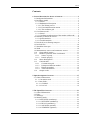
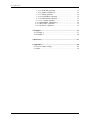
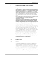
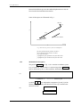
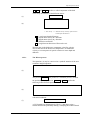
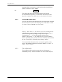
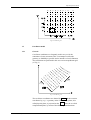
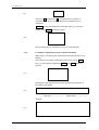
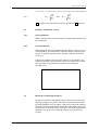
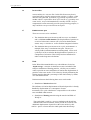
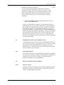
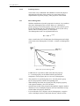
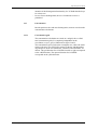
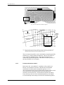
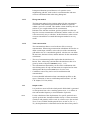
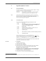
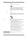
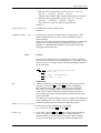
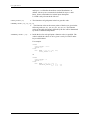
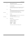
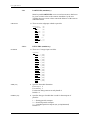
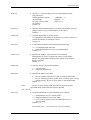
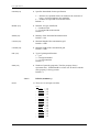
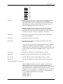
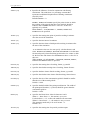
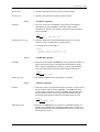
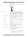
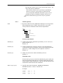
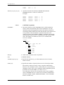
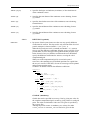
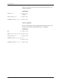
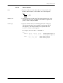
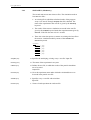
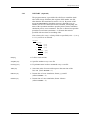
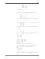
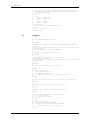
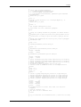
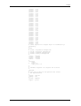
User’s Guide
SIMPAR
SIMONA
report number 98-02
User's Guide
SIMPAR
calculates the displacement of particles in a
two-dimensional water flow environment.
SIMPAR
Version
Maintenance
Copyright
:
:
:
10.43, January 2008
see www.helpdeskwater.nl/waqua
Rijkswaterstaat
Contents
Contents
1 General directions for the use of SIMPAR.................................... 3
1.1 Background information.......................................................... 3
1.2 Rectilinear model .................................................................... 3
1.2.1 General............................................................................ 3
1.2.2 Mathematical description ................................................. 4
1.2.2.1 The Wiener process ..................................................... 5
1.2.2.2 Fractional Brownian motion ........................................ 6
1.2.2.3 The rectilinear grid ...................................................... 6
1.3 Curvilinear model ................................................................... 7
1.3.1 General............................................................................ 7
1.3.2 Coordinate transformation of the random walk model........ 8
1.4 Boundary treatment in SIMPAR ................................................ 9
1.4.1 Open boundaries: ............................................................. 9
1.4.2 Closed boundaries:........................................................... 9
1.5 Dissolved versus floating transport.......................................... 9
1.6 Involved files ........................................................................ 10
1.7 Simulation time span............................................................. 10
1.8 Wind .................................................................................... 10
1.9 Momentaneous sources and continuous sources ..................... 11
1.10
Geographical aspects...................................................... 11
1.11
Release of particles in the environment ........................... 11
1.11.1 Source or group......................................................... 11
1.11.2 Particle property........................................................ 12
1.12
Mass disintegration ........................................................ 12
1.13
Concentration................................................................. 13
1.13.1 Concentration grid..................................................... 13
1.13.2 Pointspread function method...................................... 14
1.13.3 Histogram method ..................................................... 15
1.13.4 Total concentration.................................................... 15
1.14
Output results ................................................................ 15
2 Input description of SIMPAR ..................................................... 17
2.1 General information .............................................................. 17
2.1.1 Conventions used ........................................................... 17
2.1.2 Data fields ..................................................................... 18
2.1.2.1 GLOBAL.................................................................. 18
2.1.2.2 LOCAL .................................................................... 19
3 The Input File of SIMPAR .......................................................... 21
3.1 General Information.............................................................. 21
3.2 Echo..................................................................................... 21
3.3 Warnings.............................................................................. 21
3.4 Main keywords ..................................................................... 21
3.4.1 PARTICLES (mandatory).............................................. 22
3.4.1.1 INTEGERS (mandatory)........................................... 22
3.4.1.2 REALS (mandatory) ................................................. 24
3.4.1.3 SOURCES (optional) ................................................ 27
3.4.1.4 NUMBERS (optional)............................................... 27
Version 10.43, January 2008
i
User’s guide SIMPAR
3.4.1.5 TRACKS (optional) .................................................. 27
3.4.1.6 TIMES (mandatory).................................................. 28
3.4.1.7 WIND (optional) ....................................................... 29
3.4.1.8 CONTSRCS (optional) ............................................. 30
3.4.1.9 DIFFUSION (optional) ............................................. 31
3.4.1.10 MASS (optional) .................................................. 33
3.4.2 SDSNAMES (Mandatory) ............................................ 34
3.4.3 RESTART (Optional) ................................................... 35
3.4.4 OUTPUT (Optional) ..................................................... 36
4 Examples ................................................................................... 37
4.1 Example 1 ............................................................................ 37
4.2 Example 2 ............................................................................ 40
5 References ................................................................................. 47
6 Appendices ................................................................................ 49
6.1 List for further reading.......................................................... 49
6.2 Index .................................................................................... 49
ii
Input description of SIMPAR
1
General directions for the use of SIMPAR
1.1
Background information
SIMPAR simulates
the transport of floating particles and particles that
behave like dissolved substances. It is an off-line program that calculates the movement of particles in two dimensions due to advection,
diffusion and wind. Transport of particles by advection is based on a
water movement model and is computed by interpolation fom the
water velocities. SIMPAR uses the same grid as the water movement
model.
In this section a concise mathematical description of SIMPAR is given.
A more detailed description will be part of the technical
documentation of SIMPAR.
The Directorate-General for Public Works and Water Management
frequently uses transport models to calculate the effects of different
discharging sources on surface waters. Policy plans and disasters may
be computationally validated with it. Matter transport of different
compositions may be simulated with the so called particle model.
There are two possibilities for this particle model:
a random walk model or a fractional Brownian motion.
The particle model is based on a stochastic differential equation. The
equation contains two parts, a drift part and a diffusion part. The drift
part is related to the water flow and the bottom topography. The
relevant data are given by the WAQUA water movement model in an
SDS file. The diffusion part is a stochastic model: the particle makes
random jumps in the direction of the water flow or in a direction
perpendicular to it. The size of the jump is determined by chance.
In a random walk model the diffusion part is based on the Wiener
process where the spreading of particles grow linearly with time.
In a fractional Brownian motion the diffusion part is based on the so
called fractional Brownian motion where the spreading of particles
varies in time. The user can choose either the random walk model or
fractional Brownian motion for the simulation.
1.2
Rectilinear model
1.2.1
General
To model advection-diffusion the movement of a single particle is
insignificant, but the movement of a large collection of particles
undergoing drift and random motion, is significant. The displacement
of a particle by drift is determined by a time integration of the WAQUA
given flow velocity and the gradients of the bottom topography. The
random displacement is based on the so called Wiener process, in
which the particle undergoes a longitudinal (in the direction of flow)
as well as a transversal deviation. To this end a random number is
drawn for each direction from a probability distribution.
Version 10.43, January 2008
3
User’s guide SIMPAR
Instead of the Wiener process the random displacement can also be
based on the fractional Brownian motion.
Some of the aspects are illustrated in Fig. 1.
(Xt,Yt)
[3]
[2]
y
[1]
direction of flow
(Xt0,Yt0)
x
Fig. 1 Movement of a particle by advection and diffusion.
(Xt0,Yt0) position of the particle at time to
(Xt,Yt) position of the particle at time t
[1] advection part
[2] diffusion part parallel to the flow direction
[3] diffusion part normal to the flow direction
1.2.2
Mathematical description
The position
(see Fig. 1) in a cartesian coordinate system
(x,y) of a particle, which at time t0 is injected at position
,
may be described by the so called stochastic differential equations:
(1)
drift part
diffusion part
in which
,
are independent components [2] and [3] of the
Wiener process parallel to the direction of flow resp. normal to the
direction of flow:
(2)
4
Input description of SIMPAR
,
and
,
are the so called components of the drift
vector resp. the elements of the diffusion matrix:
(3)
(4)
flow velocity
additional velocity caused by spatial variation
of water depth and diffusion
= total water depth till bottom
= depth mean velocity in x-direction
= depth mean velocity in y-direction
D = diffusion coefficient
= angle between direction of flow and x-axis
The first term in the driftvector components is the flow velocity.
The second term in the driftvector components is an additional
velocity as a consequence of spatial variation of water depth and
diffusion.
1.2.2.1
The Wiener process
The equations (1) may be conceived as a symbolic notation of the next
stochastic integral equations:
(5)
The position
of the particle is a stochastic process, in which
the probability density function
for
satisfies the
following Fokker-Planck equation:
(6)
with initial condition:
(7)
A.W. Heemink has demonstrated (cf. Ref. 1), that there exists a
relation between the probability density p satisfying the Fokker-Planck
Version 10.43, January 2008
5
User’s guide SIMPAR
equation and the concentration c in the Eulerian advection diffusion
eqation, as used in WAQUA, namely:
(8)
This means that the particle movement satisfies the Eulerian
advection-diffusion equation, i.e. both models start from the same
physical assumptions, the differences are only numerical in nature.
1.2.2.2
Fractional Brownian motion
The user can choose for the diffusion part to be based on the fractional
Brownian motion in stead of the Wiener process. This choice is made
by means of keyword IHURST. (see User Input)
…
…
…
When ½ < hurst factor < 1, the motion is persistent, meaning that the
probability that a particle continues to move in the same direction it
came from is large; the spreading of the particles is larger.
For hurstfactor = ½ , we have the random walk movement.
When 0 < hurst factor < ½ , the motion is anti-persistent, meaning
that the probability that a particle will choose a different direction than
the one it came from is increased; the spreading is smaller.
For more detailed information about concentration profiles see the
report “The modeling of Diffusion in Particle Models” (cf. Ref. J.W.
Stijnen, H.X.Lin (2000))
1.2.2.3
The rectilinear grid
The rectilinear grid on which SIMPAR makes its calculations, is
furnished by WAQUA. It looks as follows (see User’s Guide WAQUA)
6
Input description of SIMPAR
Fig. 2 Rectilinear grid
1.3
Curvilinear model
1.3.1
General
Curvilinear coordinates are frequently used in WAQUA for the
simulation of water movement. This is an attempt to reflect the
geometry as faithfully as possible and to introduce a local refinement.
The calculations are performed in this case on a non-equidistant grid
(cf. Fig. 3)
g
g
Fig. 3 Curvilineair grid
The curvilinear coordinates are denoted by
and the cartesian
coordinates by (x,y). A geometry in the cartesian (x,y)-plane, also
called physical plane, is projected on the
plane, the so called
computational plane, by means of the following transformations:
Version 10.43, January 2008
7
User’s guide SIMPAR
(9)
The curves = constant and = constant build two systems of
coordinate lines. WAQUA requires that these coordinate lines are
orthogonal.
Are the transformation coefficients of the (x,y)-cartesian
system to the
-curvilinear system.
(10)
The curvilinear grid is furnished by WAQUA (in the SDS-file).
1.3.2
Coordinate transformation of the random walk model
When using a curvilinear grid, the mathematical equations have to be
adapted.
The relations between the components of the water velocity
the (x,y)-plane and the components
given by:
in the
in
-plane are
(11)
Substitution of the transformations gives the following equations of
the random walk model:
(12)
drift part
in which:
(13)
8
diffusion part
Input description of SIMPAR
flow velocity
(14)
additional velocity caused by spatial variation of water depth and diffusion
G11 =
2D
g
and
G 22 =
2D
g
= angle between the direction of flow and the local
1.4
Boundary treatment in SIMPAR
1.4.1
Open boundaries:
-direction
When a particle passes an open bounary it is halted and removed from
the calculations.
1.4.2
Closed boundaries:
When during the advective displacement the particle is about to pass a
closed boundary, the calculation is renewed with half a timestep. This
process is repeated, until the particle remains within the model area
(see Fig. 4).
If during the random step the particle would cross the boundary, the
particle is put back to its old position and a new random step is made.
This procedure is repeated until the particle stays within the
simulation area.
Fig. 4 Particle trajectory along the coast by halving the timestep
1.5
Dissolved versus floating transport
In SIMPAR an option is introduced to discern between ‘dissolved’ and
‘floating’ transport of a particle. The choice is made by means of the
keyword IMODEL (see User Input). In the case of dissolved transport
the spatial variation of the dispersion and the water depth is taken into
account. This is reflected in the second term of the drift components in
equations (13). In the case of floating transport it is not taken into
account.
Version 10.43, January 2008
9
User’s guide SIMPAR
1.6
Involved files
SIMPAR utilizes it’s own SDS files. In this file all necessary data is
stored and will be used for postprocessing activities. A subset of this
data has been generated by SIMPAR (e.g. position of particles) and
another subset is copied from the WAQUA SDS file (e.g. geometry and
water levels). WAQUA information that is actually used in a WAQUA
computation, but not necessarily used for post processing purposes, is
only read from a WAQUA SDS file but not copied.
1.7
Simulation time span
There are two cases to be considered:
The simulation time span in SIMPAR and in WAQUA are identical
and is called the actual situation. The displacement of particles as
a result of advection in SIMPAR will be based on both momentaneous WAQUA velocities as well as Eulerian integrated velocities.
The simulation time span in SIMPAR in a cyclic environment is a
multiple of the WAQUA simulation time span . The WAQUA
velocity fields (both momentaneous and integrated) can be used
cyclically in order to calculate the displacement of particles as a
consequence of advection. This facility has been introduced in
order to make long term calculations.
1.8
Wind
In the Water Movement Model WAQUA the influence of wind on
‘depth average’ velocities is taken into account. On behalf of the
transport simulation of floating particles, a facility was created in
order to provide an extra contribution of wind on the displacement of
particles at the water surface. This is done by directly influencing the
floating particles through a percentage of the wind velocity by means
of a user defined factor.
Distinction between the following three cases can be made:
Simulation of dissolved material:
The influence of wind on displacement of dissolved particles is already
handled by displacement as a consequence of water
movements. In a cyclic calculation it is impossible to work with an
extra windfield within SIMPAR.
Simulation of floating material using the actual wind fields of
WAQUA:
The wind which is used by a WAQUA simulation and already has
influenced the water movement, will be passed on to SIMPAR. The
additional displacement of particles at the water surface by this
wind is e qual to a factor times the wind speed times the timestep.
10
Input description of SIMPAR
This factor is specified by the user.
Note:
In case of space varying wind, the wind can not be directly
passed on to SIMPAR. Therefore the user has to specify a wind
SDS-file, from which SIMPAR can obtain the needed wind values.
It is the responsibility of the user that (s)he specifies the same
wind SDS-file as used in WAQUA, because SIMPAR is unable to
check this.
Simulation of floating material combined with cyclical use of
WAQUA fields within SIMPAR.
In the case of tidal water movements a varying wind may be used.
While the wind in WAQUA is only available over a restricted period of
time (a tide), this wind variation in time (but uniform in space) has to
be introduced in SIMPAR by a time sequence of winds, or in case of
space varying wind by a wind SDS-file. The wind driven displacement
at the water surface will again be specified by a user given factor times
the wind speed times the timestep. The user has to take notice of the
fact that it is not allowed to create or use WAQUA fields with wind
involved, if those fields are used in a later stage in cyclical calculations
of a SIMPAR simulation.
1.9
Momentaneous sources and continuous sources
A simulation with SIMPAR can be based on momentaneous sources as
well as continuous sources. Momentaneous sources are the ones where
all particles are released simultaneously. Continuous sources are
characterised by a continous release of particles during a certain time
period, which may vary in intensity.
1.10
Geographical aspects
The position of the sources is represented by geographical coordinates
(x,y) with Paris as point of reference. In SIMPAR these coordinates are
transformed to model (n,m) coordinates. The transformation to
spherical coordinates is not yet implemented.
1.11
Release of particles in the environment
1.11.1
Source or group
Particles are released in groups. From a certain geographical position
more than one group of particles might be released. One group may
contain a variable number of particles.
Version 10.43, January 2008
11
User’s guide SIMPAR
1.11.2
Particle property
has arrays (PROPAR and GRPROP) in which the physical
and chemical properties of the particles are stored. Only mass is
implemented as a particle propery, other properties can de added.
SIMPAR
1.12
Mass disintegration
With the introduction of particle properties in SIMPAR, it is possible to
take mass disintegration into account. Mass (m) is defined as a
particle property. The initial property value (the mass) must be given
by the user and also the rate of disintegration is given by the user by
means of the TCHAR keyword. (see User Input)
The disintegration itself is an exponential decrease,
m
m0 e
tchart
where a small value for TCHAR means fast disintegration and a high
value means slow disintegration. TCHAR = 0 means no disintegration
at all.
Illustration of mass disintegration
Furthermore it is possible to define more than one property.
I.e. a second property can be defined which represents the
temperature. Each property has its own rate of disintegration.
NOTES
12
– The properties are specified groups wise. So each particle group
has its own properties with the corresponding rates.
When defining more than one property the first property (property
with sequence number 1) has to be the mass.
SIMPAR keeps record of the properties through their sequence number.
Therefore in case of multiple properties, the user himself has to keep
in mind what each property stands for.
It is not allowed to use a negative rate of disintegration. A negative
value would imply increase rather than decrease, which is not the
Input description of SIMPAR
intention of the disintegration functionality. So TCHAR should always
be at least zero.
In case of mass disintegration, the use of continuous sources is
prohibited.
1.13
Concentration
Besides particle tracks and mass disintegration, SIMPAR can also make
concentration calculations.
1.13.1
Concentration grid
The concentration calculations are made on a subgrid, the so called
total concentration grid (G1) completely independent on the
(curvilinear) WAQUA grid, as illustrated in figure 5 and 6.
The concentration grid is laid on the rectangular area, where the small
square grid space size CELLDX in meters is chosen, and the number
of grid spacves in the two dimensions, CONLEN and CONWID, are
chosen. The grid direction for CONLEN from left to right corresponds
to the x-RD-direction. The upward direction for CONWID
corresponds to the y-RD-direction.
Version 10.43, January 2008
13
User’s guide SIMPAR
CONWID
CONLEN
DETAIL
y
x
Fig. 5 Overview of the total concentration grid G1
WAQUA grid
Concentration
grid (G1)
celldx
particle
Grid of
particle i
(G2)
celldx
i
2 * psfwid
Fig. 6 Overview of the structure of the grid G2(i) for particle I where the spread function is
defined. Each particle lies in the center of its own G2(i). The particle positions are
rounded to the bottm left corner of the small squares of G1.
These concentration profiles can be calculated by using histogram-like
functions or by using pointspread functions. The user can choose to
run a simulation with histograms, with pointspread functions or
without any concentration profiles. This choice is made by means of
the keyword IPSF (see User Input).
1.13.2
Pointspread function method
But because the “exact physical” coordinates of the particles are
known, it is beneficial to use these. Therefore the concentration
calculations are made on the concentration grid (see 1.13.1).
This concentration grid is based on the particle positions of the current
time. Because this concentration grid is based on the particle
positions, it has no fixed size. As the cloud of particles can change
every time-step, the size of the concentration grid may also change.
For each timestep SIMPAR keeps record of the concentration gridsize.
14
Input description of SIMPAR
Pointspread functions spread the mass of a particle across
neighbouring gridcells, wich results in a much smoother and more
accurate concentration than when using histograms.
1.13.3
Histogram method
The histogram method is the simplest method for the concentration
calculations. With the histogram method the number of particles
withtin a grid cell is counted. This number is than divided by the cell
surface to get a rough estimate for the concentration.
Problems arise with the curvilinear grid: the gridcells are often too
large for accurate concentration calculations, and the surface of a cell
is not necessearily easy to calculate. In this situation or when a more
accurate concentration is wanted the histogram method is not very
useful.
1.13.4
Total concentration
The concentrations that are saved to the SDS file are average
concentrations. When using concentration calculations the user has to
define certain input variables, such as the size of the concentration
grid and the size of a concentration gridcell. Also the user can define
the start time, the interval time, and the end time for the concetration
calculations.
NOTES
– The use of concentration profiles implies that the initial mass is
known. Thus, when using concentrations the initial mass has to be
given by means of keyword GRPROP (see § 1.11.2).
– The concentrations functionality can be used in combination with
mass disintegration. If only concentrations are required and no mass
disintegration the keyword TCHAR has to be set to zero.
– Continuous sources may not be used in combination with
concentrations!
For more detailed information about concentration profiles see the
report “Extension of SIMPAR with Pointspread Functions” (cf. Ref.
J.W. Stijnen, H.X.Lin (2000))
1.14
Output results
It is possible to store in file the whole particle field which is generated
at some point of time. Also a tracking option exists, i.e. to follow in
time with another frequency a selected number of particles.
NOTE
Version 10.43, January 2008
For the calculation of the displacement of a specific particle from a
specific point in time, the next available velocity of water movement,
waterlevel and geometry will be used. So, when WAQUA data at times
T0 en T1 are available and the particle leaves at time td (T0 < td <
T1), the displacement is calculated based on the data at time point T1.
15
Input description of SIMPAR
2
Input description of SIMPAR
2.1
General information
The input is based on SIMONA KEYWORD structure. Refer to "About
"General Information".
Reminder:
The input file is a structured ASCII-file. From the
input file only the first 120 columns are read.
SIMONA" in Section 1
Note:
If the last keyword block in the input file contains a sequential
keyword, the SIMONA application independent preprocessor is not
able to check the correctness of the block. This can result in
incorrect processing of the input file!
2.1.1
Conventions used
For the input definition the following conventions are used:
[val]
:
real value1
[tval]
:
time specification in the form: day hours:minutes (e.g.
2 21:15). Times are given relative to midnight of a
reference date, starting at 0 0:00.
[ival]
:
integer value
[iseq]
:
sequence number to indicate a point, curve, etc.
[text]
:
string (enclosed between quotes)
< ... >
:
repetition group
|A
<
:
choice between A and B (A and B are mutually exclusive)
|B
&
:
continuation mark
In this document keywords are partly underlined (e.g., PRINTOUTPUT).
Only the underlined characters are significant. So the user must type
at least PRINT in his input, but PRINTOUT is accepted as well.
The 'Explanation' part of the description of the various sections and
subsections is divided in three columns:
KEYWORD
E
O
M
D
S
R
X
Explanation
E can be O, M, D, S, R, X.
means keyword is optional.
means keyword is mandatory.
means keyword has a default value. When this keyword is omitted,
the pre-processor will use the default value for the variable
specified by means of this keyword.
means this keyword is a sequential keyword: a keyword followed by
an integer (e.g. P4). A sequential keyword can be used repeatedly.
means keyword may occur more than once.
Exactly one of a series of keywords should be given.
1
Since all values are read in free format: integer notation (when reals are expected) will be converted to reals, so "val = 4" is identical to "val =
4.0".
Version 10.43, January 2008
17
User’s guide SIMPAR
2.1.2
Data fields
Data field input is to be specified in two blocks:
SPACE_VARYING_DATA
GLOBAL
LOCAL
SPACE_VARYING_DATA stands for any key-word representing
spatial data. In GLOBAL the data for the complete field is to be
given, specifying function values at all grid points. In LOCAL
however the user can specify rectangular boxes in which he can
change the value of the space varying data. For the case of 3D this
definition is extended in such a way that the input for separate layers
is possible.
2.1.2.1
GLOBAL
Global data can be specified in two ways: first by giving one value for
the complete computational grid, second by giving values for each grid
point. The order in which these values are to be given is specified by
the layout flag.
GLOBAL
LAYOUT = [ival]
| CONST_VALUE = [val]
<
| VARIABLE_VALUES = < [ival] >
LAYOUT = [ival]
D
Explanation:
Layout-indicator specifying the order in which the values from
input file are assigned to the function value in a grid point. Possible
values for LAYOUT and their meaning are:2
1. function values at grid points: [(m1,n1), (m1,n1+1) ... (m1,n2)],
[(m1+1,n1) ... (m1+1,n2)] ... [(m2,n1) ... (m2,n2)]
columns; first column is left; column values from bottom to top
2. function values at grid points: [(m1,n1), (m1+1,n1) ... (m2,n1)],
[(m1,n1+1) ... (m2,n1+1)] ... [(m1,n2) ... (m2,n2)]
rows; first row is bottom; row values from left to right
3. function values at grid points: [(m2,n1), (m2,n1+1) ... (m2,n2)], [(m21,n1) ... (m2-1,n2)] ... [(m1,n1) ... (m1,n2)]
columns; first column is right; column values from bottom to top
4. function values at grid points: [(m2,n1), (m2-1,n1) ... (m1,n1)],
[(m2,n1+1) ... (m1,n1+1)] ... [(m2,n2) ... (m1,n2)]
rows; first row is bottom; row values from right to left
5. function values at grid points: [(m1,n2), (m1,n2-1) ... (m1,n1)],
[(m1+1,n2) ... (m1+1,n1)] ... [(m2,n2) ... (m2,n1)]
columns; first column is left; column values from top to bottom
6. function values at grid points: [(m1,n2), (m1+1,n2) ... (m2,n2)],
[(m1,n2-1) ... (m2,n2-1)] ... [(m1,n1) ... (m2,n1)]
rows; first row is top; row values from left to right
2
Assume the limits of the box are given by (m1, n1) and (m2, n2) with m1 m2 and n1
and m2= MMAX. The number of required function values is then ntot*mtot, where :
ntot= (number of enclosed n grid points) = n2 - n1 +1
mtot= (number of enclosed m grid points) = m2 - m1 +1
18
n2. In the case of global input n1 =1, n2=NMAX, m1 =1
Input description of SIMPAR
7. function values at grid points: [(m2,n2), (m2,n2-1) ... (m2,n1)],
[(m2-1,n2) ... (m2-1,n1)] ... [(m1,n2) ... (m1,n1)]
columns; first column is right; column values from top to bottom
8. function values at grid points: [(m2,n2), (m2-1,n2) ... (m1,n2)],
[(m2,n2-1) ... (m1,n2-1)] ... [(m2,n1) ... (m1,n1)]
rows; first row is top; row values from right to left
Default = 1.
CONST_VALUES = [val]
O
Constant value for the complete field.
Default = 0.
VARIABLE_VALUES = < [val] >
O
It is possible to specify a function value at each grid point . The
order in which the values are to be given is defined by means of
layout-indicator.
In the case of 3D the information must be specified as a set of KMAX
separate layers, each layer given according to the global layoutindicator (i.e. MMAX*NMAX*KMAX values must be specified,
beginning with the top layer) .
2.1.2.2
LOCAL
In LOCAL the function values at grid points specified in GLOBAL
can locally be overwritten by specifying boxes (i.e. rectangles). In the
3D-case a box is a rectangle drawn in the horizontal plane identified
by the layer-index.
LOCAL
< BOX: MNMN = ( [ival], [ival] ) ( [ival], [ival] ) LAYER = [ival]
| CONST_VALUES = [val]
<
| CORNER_VALUES = [val], [val], [val], [val]
<
| VARIABLE_VALUES = < [val] >
BOX
R
Explanation:
A BOX is defined by specifying its opposite corner points (m1,n1)
and (m2,n2), where m1 m2 and n1 n2. In this rectangle the
global function value of a "field" variable can be overwritten by
new values. It is possible to define more than one box for one
single "field" variable. When the rectangles defined in the boxes
have common grid points, the latest values specified for those grid
point will be used.
The data can be specified either by means of a single value defining all
points within the box or by means of a array of data. In the latter case
the data should be given according to the following scheme:
MNMN = ( [ival], [ival] ) ( [ival], [ival] )
LAYER = [ival]
Version 10.43, January 2008
M
Corner points of the rectangular box, specifying
(m1, n1) (m2, n2), where m1 m2 and n1 n2.
O
Layer index , where 0 layer kmax. If layer is not specified or
layer=0, a uniform vertical distribution is assumed. However,
when the function values belong to a data-array which is defined
for layers 0 until kmax, layer=0 is only valid for the upper layer
19
User’s guide SIMPAR
and layer=-1 will define the uniform vertical distribution. As
default, 3D-arrays are assumed to be defined for layers 1 until
kmax, unless stated otherwise in their input description.
LAYER is only relevant in the 3D-case.
CONST_VALUES = [val]
O
The function at all grid points in the box gets this value.
CORNER_VALUES = [val], [val], [val], [val]
VARIABLE_VALUES = < [val] >
O
The function values at the corner points of the box are given in the
following order (m1, n1), (m2, n1), (m2, n2), (m1, n2). The function
values at the other grid points enclosed by the box will be determined
by means of bilinear interpolation.
O
Inside the box for each grid point a function value is specified. The
order in which the values are to be given is set by LAYOUT under
key-word GLOBAL.
For example:
GLOBAL
CONST_VALUES = 40.5
LAYOUT = 4
LOCAL
BOX: MNMN = (10, 5), (50, 100)
CONST_VALUES = 38
or
GLOBAL
CONST_VALUES = 0
LAYOUT = 3
LOCAL
BOX: MNMN = (10, 5), (11, 7)
VARIABLE_VALUES = 2 2.3
1.9
2.0
20
2.4
3.2
The Input File of SIMPAR
3
The Input File of SIMPAR
The input of the SIMPAR program is described in this chapter.
3.1
General Information
For general information about the conventions being used for the data
fields the reader is referred to section 2.1.1 of this user’s guide.
3.2
Echo
The first statement in the input file may set the echo environment. This
means that the contents of the input file will or will not be sent to the
user’s standard output (in general: the message file).
Tell SIMPAR that no echo of input file contents is needed.
SET NOECHO
3.3
Warnings
The number of warnings in the message file may be restricted to a user
defined number. Default is 10.
Sets the number of warnings in the message file.
SET MAXWARN
3.4
Main keywords
The input is divided into 4 main keywords
PARTICLES (Mandatory)
SDSNAMES
(Mandatory)
RESTART
(Optional)
OUTPUT
(Optional)
These keywords are described in the following sections.
Version 10.43, January 2008
21
User’s guide SIMPAR
3.4.1
PARTICLES (mandatory)
Main keyword PARTICLES covers several KEYWORDs that has to
be given as initial values to the SIMPAR-simulation by the user.
Together these KEYWORD values control the behavior of the SIMPAR
simulation model.
PARTICLES
M
There are nine subgroups related to particles.
PARTICLES
(M)
INTEGERS (M)
REALS
(M)
SOURCES
(O)
NUMBERS
(O)
TRACKS
(O)
TIMES
(M)
WIND
(O)
CONTSRCS (O)
DIFFUSION (O)
3.4.1.1
INTEGERS
INTEGERS (mandatory)
M
There are 17 integer input variables.
INTEGERS
NDIM
IMODEL
IBCK
ITPAR
NPARG
ISTEP
NPTRAC
IMOVE
IFIELD
IVELO
DATIME
IHURST
MEMO
CONLEN
CONWID
IPSF
PDIM
=
=
=
=
=
=
=
=
=
=
=
=
=
=
=
=
=
[ival]
[ival]
[ival]
[ival]
[ival]
[ival]
[ival]
[ival]
[ival]
[ival]
[ival]
[ival]
[ival]
[ival]
[ival]
[ival]
[ival]
NDIM=[ival]
D
Specifies the model dimension.
For WAQUA: 2
For TRIWAQ: 3
For the time being SIMPAR can only handle 2.
Default = 2
IMODEL=[ival]
D
Specifies the type of model that is used for the transport of
particles:
1 = floating particle transport
2 = dissolved particle transport
3 = suspended particle transport (not yet implemented)
Default = 1
22
The Input File of SIMPAR
IBCK=[ival]
D
Specify = 1, if backtracking (reverse in time) should be done.
Only allowed if:
floating particle transport
(IMODEL = 1)
advection only
(IMOVE = 1)
no cyclic velocity fields
(IVELO 3)
no restart(s)
Default = 0
ITPAR=[ival]
D
Specifies the maximum number of iterations executed per time step
and per particle. It is recommended to use the value 2.
Default = 3
NPARG=[ival]
O
Specifies the number of particle groups.
It’s equivalent to the number of momentaneous sources. It does not
include the number of continuous sources.
Default = 0
ISTEP=[ival]
D
Is an indicator related to the calculation of the time step:
0 = user defined (fixed) time step
1 = program determines time step (not implemented)
Default = 0
NPTRAC=[ival]
D
Specifies the number of particles that will be tracked.
Subsequently for NPTRAC particles the status of each distinct
particle, the group number of the particle and the serial number
must be specified.
Default = 0
IMOVE=[ival]
M
Specifies the type of particle-movement.
1 = only advection
2 = advection and diffusion
IFIELD=[ival]
D
Specifies the kind of wind field.
0 = No extra wind in SIMPAR even if the user had specified wind.
1 = In case of floating particles, global WAQUA-wind or space varying
wind in SIMPAR. In case of cyclic fields, a user defined wind.
Default = 0
Note:
In case of space varying wind, the wind SDS filename and the
experiment name of the wind SDS must be specified
(see 3.4.1.10)
IVELO=[ival]
D
Specifies which kind of velocity field has to be selected.
1 = momentaneous WAQUA-velocity fields
2 = integrated Eulerian rest-current fields
3 = cyclic velocity fields based on momentaneous WAQUAvelocity fields
Default = 2
Note: when ivelo = 3, no restarts (see 3.4.3) are allowed.
Version 10.43, January 2008
23
User’s guide SIMPAR
DATIME=[ival]
D
Specifies the method of time specification.
1 = All times are specified relative in relation to the start time of
WAQUA in elapsed minutes after midnight.
2 = All times are specified in an absolute sense.
Default = 1
IHURST=[ival]
D
Indicator for type of diffusion.
1 = Random walk
2 = Fractional Brownian motion.
Default = 1
MEMO=[ival]
D
Memory of the fractional Brownian motion.
Default = 100
CONLEN=[ival]
D
Maximal length of the concentration grid.
Default = 1000
CONWID=[ival]
D
Maximal width of the concentration grid.
Default = 1000
IPSF =[ival]
D
Type of pointspread function.
1 = psf
2 = histogram method
3 = no concentrations
Default = 3
PDIM=[ival]
D
Number of particles properties. The first property always
represents mass. PDIM should be at least one. In other words the
mass property is always present.
Default = 1
3.4.1.2
REALS
REALS (mandatory)
M
There are 19 real input variables.
REALS
TSTEP
TIPARW
| TFPARW
| TLPARW
<
| DATFPW
| TIMFPW
| DATLPW
| TIMLPW
PARAA
PARAB
PARAC
WOPFAC
TITRAC
| TFTRAC
| TLTRAC
<
24
=
=
=
=
[val]
[val]
[val]
[val]
=
=
=
=
=
=
=
=
=
=
=
[val]
[val]
[val]
[val]
[val]
[val]
[val]
[val]
[val]
[val]
[val]
The Input File of SIMPAR
|
|
|
|
TSTEP=[val]
M
DATFTW
TIMFTW
DATLTW
TIMLTW
CELLDX
PSFWID
HURST
TFCONC
TFCONC
TLCONC
=
=
=
=
=
=
=
=
=
=
[val]
[val]
[val]
[val]
[val]
[val]
[val]
[val]
[val]
[val]
Specifies the time step that is used for SIMPAR simulations. During
the simulation process SIMPAR adapts time steps constantly to
output requirements: SIMPAR synchronizes those time intervals in a
sense that output is always available when it is needed. So, there is
no need for interpolation between two intervals.
TFPARW, TIPARW and TLPARW specify writing times to disk of
particles positions relative to the start of the WAQUA-simulation,
respectively first time, time interval and when to write last. DATIME
must have a value of 1 in this case, explicitly or by default.
TFPARW=[val]
O
Specifies the first writing time of particle positions relative to the
start of the simulation.
TIPARW=[val]
M
Specifies the time interval of writing.
TLPARW=[val]
O
Specifies the last writing time of particle positions relative to the
start of the simulation.
As an alternative the user also can specify absolute datum’s and times.
DATFPW and TIMFPW, DATLPW and TIMLPW are in time/date
format and specify when all particles positions must be written to disk
for the first time and when last. DATIME must have a value of 2 in
this case.
DATFPW=[val]
O
Specifies the starting date of writing; format yyyymmdd.
TIMFPW=[val]
O
Specifies the absolute starting time of writing; format hhmmss.
DATLPW=[val]
O
Specifies the date when to finish writing; format yyyymmdd.
TIMLPW=[val]
O
Specifies the absolute time when to finish writing; format hhmmss.
PARAA=[val], PARAB=[val], PARAC=[val] D
PARAA, PARAB and PARAC
specify the standard deviation of the
random displacement of a particle in respectively the horizontal
velocity direction, in a velocity direction perpendicular to this direction
in the horizontal plane, and in the vertical direction. It can be
interpreted as an XYZ-system or a 3-dimensional system. The vertical
direction is not yet operational. (As an indication of magnitude the
WAQUA diffusion coefficient may be selected.)
Default PARAA = 0.
Default PARAB = 0.
Default PARAC = 0.
Version 10.43, January 2008
25
User’s guide SIMPAR
WOPFAC=[val]
D
Specifies the influence of wind in conjunction with floating
constituents. The wind factor is a percentage constant that
represents an additional displacement of floating constituents
caused by wind.
Default WOPFAC = 0.
TFTRAC, TITRAC and TLTRAC specify the points in time at which
the positions of the particles that have been tracked, should be
written to disk. DATIME must have a value of 1 in this case,
explicitly or by default.
When NPTRAC > 0 and DATIME = 1, TFTRAC, TITRAC and
TLTRAC must be specified.
TFTRAC=[val]
O
Specifies the starting time point of particles tracking in minutes
after the start of the simulation.
TITRAC=[val]
O
Specifies the time interval in minutes.
TLTRAC=[val]
O
Specifies the time when to finish particles tracking in minutes after
the start of the simulation.
As an alternative the user also can specify absolute datum’s and
times. DATFTW and TIMFTW, DATLTW and TIMLTW are in date/time
format and specify when all tracking positions have be written to disk
for the first time and when at last. DATIME must have a value of 2 in
this case.
When NPTRAC > 0 and DATIME = 2, DATFTW, TIMFTW, TITRAC,
DATLTW and TIMLTW must be specified.
DATFTW=[val]
O
Specifies the starting date of tracking; format yyyymmdd.
TIMFTW=[val]
O
Specifies the absolute starting time of tracking; format hhmmss.
DATLTW=[val]
O
Specifies the date when to finish tracking; format yyyymmdd.
TIMLTW=[val]
O
Specifies the absolute time when to finish tracking; format hmmss.
CELLDX=[val]
D
Specifies the size of the concentration gridcell. Should be smaller
than the size of the normal gridcell.
Default = 100.0.
PSFWID =[val]
D
Specifies the half width of the pointspread function. The width of
the pointspread function (2 * psfwid) should be greater than the
concentratin gridsize.
Default = 300.0.
HURST=[val]
D
Specifies the Hurst factor. Must be between 0 and 1.
When ½ < hurst factor < 1, the motion is persistent.
For hurstfactor = 0.5, we have the random walk movement.
When 0 < hurst factor < ½ , the motion is anti-persistent.
This parameter needs only to be set if IHURST = 2.
Default = 0.5.
TFCONC=[val]
O
Specifies the starting time for particle position output.
26
The Input File of SIMPAR
TICONC=[val]
O
Specifies the interval time for particle position output.
TLCONC=[val]
O
Specifies the end time for particle position output.
3.4.1.3
SOURCES
SOURCES (optional)
O
The next KEYWORD is SOURCES. It specifies for each distinct
momentaneous group (NPARG), where the origin in model
coordinates is situated. The number of groups of sources must be
equal to NPARG.
SOURCES
< XYZCRD = ([val] , [val] , [val] ) >
XYZCRD=([val],[ val],[ val])
M
Specifies the position of the momentaneous sources, in meters
relative to Paris. NPARG must be greater than 0.
For example, in case NPARG = 2:
SOURCES
XYZCRD=( 51250.00, 405750.00, 25.)
XYZCRD=( 51150.00, 405700.00, 20.)
3.4.1.4
NUMBERS
NUMBERS (optional)
O
By means of KEYWORD NUMBERS the user specifies the number of
particles that participates in each distinct momentaneous group.
This is done by indicating two numbers : first the group number
and second the number of particles that belongs to that group.
NUMBERS
<GROUP[iseq] : [ival] >
GROUP [iseq]:[ival]
M
3.4.1.5
TRACKS
By means of GROUP the group number is specified.
TRACKS (optional)
O
If the user wants to activate the tracking of particles, he/she can do
this by means of the KEYWORD TRACKS. If NPTRAC has been
given a value greater than 0, then for NPTRAC particles the status
of each distinct particle must be specified. This means that per
particle the group number and the local number must be given.
TRACKS
< GRELMT[iseq] : [ival] >
GRELMT[iseq]:[ival]
Version 10.43, January 2008
M
By means of GRELMT the user specifies a sequential number of a
specific group and the particle number of that group. Groups are
numbered sequentially, first all momentaneous sources, followed by
all continuous sources.
27
User’s guide SIMPAR
3.4.1.6
TIMES
TIMES (mandatory)
M
On behalf of TIMES the user can specify the start- and stop time of
the particle computation.
TIMES
| COMP [val, val]
| TSTOP_WAQCYCLE = [val]
<
| STDATE = [val]
| STTIME = [val]
| ENDATE = [val]
| ENDTIM = [val]
| ENDAT_WAQCYCLE = [val]
| ENTIM_WAQCYCLE = [val]
COMP[val], [val]
O
By means of the KEYWORD COMP and two points of time,
respective start time and end time, the particle computation period
is assigned. As an alternative, the user also can specify absolute
datum’s and times. STDATE and STIME, ENDATE and ENDTIM
specify respective absolute start time and end time. DATIME must
have a value of 2 in this case.
TSTOP_WAQCYCLE =[val]
O
Specifies the relative end time (elapsed minutes after midnight of
the WAQUA-start date) of the WAQUA-cycle in case of cyclic
WAQUA-velocity fields (datime = 1 and ivelo = 3, see § 3.4.1.1).
Default: last WAQUA-map time.
STDATE=[val]
O
Specifies the start date of particle computation; format yyyymmdd
STTIME=[val]
O
Specifies the absolute start time of particle computation; format
hhmmss.
ENDATE=[val]
O
Specifies the date when to finish particle computation; format
yyyymmdd.
ENDTIM=[val]
O
Specifies the absolute time when to finish particle computation;
format hhmmss.
ENDAT_WAQCYCLE =[val]
O
Specifies the absolute date of the end of the WAQUA-cycle in case
of cyclic WAQUA-velocity fields (datime = 2 and ivelo = 3, see §
3.4.1.1). Format yyyymmdd.
Default: last WAQUA-map time.
ENTIM_WAQCYCLE =[val]
O
Specifies the absolute time of the end of the WAQUA-cycle in case
of cyclic WAQUA-velocity fields (datime = 2 and ivelo = 3, see §
3.4.1.1). Format: hhmmss.
Default: last WAQUA-map time.
Note 1: The end (date and) time must be greater than the start (date
and) time, otherwise an error will be reported and the
program stops.
Note 2: At cyclic WAQUA-velocity fields (ivelo = 3, see § 3.4.1.1),
28
The Input File of SIMPAR
the start time of the WAQUA-cycle is always the same as the
start of the SIMPAR-simulation.
The end time of the WAQUA-cycle may be specified by
the user (see above). It must fall at or before the last
WAQUA-map time. When the end of the WAQUA-cycle is
reached, the SIMPAR-simulation continues with WAQUAvelocities situated one step after the WAQUA-cycle start
time.
3.4.1.7
WIND
WIND (optional)
O
By means of the KEYWORD WIND the windaspects are incorporated
in the simulation process. Wind is only relevant in case cyclic
velocity fields in combination with wind are implemented.
WIND
WSPEED = [val]
WANGLE = [val]
WCONVF = [val]
| < TIMVAL [val val val] >
<
| < WNDVAL [val val val val] >
General wind situation.
WSPEED=[val]
D
Global wind speed in a dimension specified by WUNIT. See User’s
guide WAQPRE, § 2.7.3.
Default = 0.
WANGLE=[val]
D
Global wind direction, in degrees from 0 to 360. Wind direction
is measured clockwise from north, where (wind coming from) north
equals to 0 , (wind coming from) east equals 90 and so on.
Default = 0.
WCONVF=[val]
D
Wind conversion factor which is defined by the user.
Default = 1.
Wind time series.
From the time given on a certain line until the time given on the next
line wind speed and wind angles are specified. Before the first dataline the general wind situation rules. After the last data-line the wind
situation lasts until the end of the simulation.
TIMVAL [val],[ val],[ val]
O
Specifies time interval (minutes), WSPEED and WANGLE.
must have a value of 1 in this case.
DATIME
Example:
TIMVAL
TIMVAL
TIMVAL
TIMVAL
Version 10.43, January 2008
1000.
1600.
2000.
3000.
1.
1.
1.
1.
90.
70.
45.
90.
29
User’s guide SIMPAR
TIMVAL
TIMVAL
WNDVAL [val], [val], [val], [val]
O
6000.
8000.
1.
2.
00.
00.
Specifies absolute date and time, WSPEED and WANGLE.
have a value of 2 in this case.
DATIME must
Example:
WNDVAL
WNDVAL
WNDVAL
WNDVAL
WNDVAL
WNDVAL
3.4.1.8
CONTSRCS
19890320.
19890321.
19890321.
19890322.
19890324.
19890325.
164000.
024000.
092000.
020000.
040000.
132000.
1.
2.
2.
2.
3.
2.
90.
70.
45.
90.
0.
0.
CONTSRCS (optional)
O
By means of the KEYWORD CONTSRCS the so called continuous
sources will be incorporated in the SIMPAR simulation. For each
individual group the geographical position, the number of particles
released per minute and the start time and stop time of the release have
to be specified. The total number of particles released in each
continuous group equals NPART * TIMINT. Continuous and momentaneous particle sources may be combined in the same SIMPAR simulation. The number of continuous sources is not counted in the
KEYWORD NPARG.
CONTSRCS
< SRC[iseq] >
DATA
XYZCRD
NPART
| TIMINT
<
| TISSTD
| TISSTT
| TISEND
| TISENT
= ([val] , [val] , [val] )
= [ival]
= [val val]
=
=
=
=
[val]
[val]
[val]
[val]
SRC[iseq]
S
Labels each continuous source of particles.
DATA
M
Bundels the data.
XYZCRD=([val],[ val],[ val])
M
Specifies the position (x,y,z) of the continuous source in meters,
relative to Paris.
NPART=[ival]
M
Specifies the number of particles that are to be released per minute.
The user has a choice to specify a start-, stop time and the drain
interval of the continuous source. If these times are not specified, the
continuous source will be active during the whole computation period
specified in KEYWORD TIMES (see section 3.4.1.6).
As an alternative, the user also can specify relative times (TIMINT,
value of DATIME must be 1 in this case) or absolute calendar dates
and times (TISSTD, TISSTT, TISEND and TISENT, value of DATIME
must be 2 in this case).
30
The Input File of SIMPAR
TIMINT=[val] [val]
O
Specifies the begin- and end time (in minutes) of the drain interval
of the continuous source.
TISSTD =[val]
O
Specifies the start datum of the continuous source draining; format
yyyymmdd.
TISSTT =[val]
O
Specifies the absolute start time of the continuous source draining;
format hhmmss.
TISEND= [val]
O
Specifies the end datum of the continuous source draining; format
yyyymmdd.
TISENT= [val]
O
Specifies the end datum of the continuous source draining; format
yyyymmdd.
3.4.1.9
DIFFUSION
DIFFUSION (optional)
O
By means of the keyword DIFFUSION the user may specify diffusion
coefficients for SIMPAR. This keyword is only relevant when dissolved
particle transport is chosen (imodel = 2, see § 3.4.1.1).
When the keyword DIFFUSION is omitted (and imodel = 2) , SIMPAR
tries to copy the diffusion coefficients from the WAQUA SDS-file. If not
present there, an error message will be printed and the program stops.
In the absence of WAQUA diffusion coefficients the user should here
specify the diffusion coefficients for SIMPAR, covering the whole
computational grid.
When part of the computational grid is covered at keyword
DIFFUSION, the remaining (not yet defined) positions are copied from
the WAQUA SDS-file. If this fails, also an error message will be printed
and program execution stops.
So there is no default value for the diffusion coefficients.
DIFFUSION
GLOBAL
LAYOUT = [ival]
| CONST_VALUES = ([val])
<
| VARIABLE_VALUES = < [val] >
LOCAL
< BOX: MNMN = ([ival], [ival] ) ( [ival], [ival] )
| CONST_VALUES = [val]
<
| CORNER_VALUES = [val], [val], [val], [val]
<
| VARIABLE_VALUES = < [val] >
>
GLOBAL (mandatory)
Global data can be specified in two ways: first by giving one value for
the complete computational grid, second by giving values for each grid
point. The order in which these values are to be given is specified by
the LAYOUT flag.
Although keyword GLOBAL is mandatory, no value(s) for either
CONST_VALUES or VARIABLE_VALUES need to be given for the
Version 10.43, January 2008
31
User’s guide SIMPAR
diffusion coefficients: missing values will be taken from the WAQUA
SDS-file (if present).
Explanation:
LAYOUT = [ival]
D
See § 2.1.2.1.
Default = 1.
CONST_VALUES = [val]
O
See § 2.1.2.1.
[val] > O
See § 2.1.2.1.
VARIABLE_VALUES
=<
LOCAL (optional)
In LOCAL the function values at grid points specified in GLOBAL can
locally be overwritten by specifying boxes (i.e. rectangles).
Explanation:
R
See § 2.1.2.2.
MNMN = ([ival], [ival]) ([ival], ival]) M
See § 2.1.2.2.
CONST_VALUES = [val]
See § 2.1.2.2.
BOX
O
CORNER_VALUES = [val], [val], [val], [val]
VARIABLE_VALUES
32
=<
O
See § 2.1.2.2.
[val] > O
See § 2.1.2.2.
The Input File of SIMPAR
3.4.1.10
MASS
MASS (optional)
O
By means of the KEYWORD MASS the user can specify for each
group the initial property values and the rate of disintegration.
MASS
GRPROP = [val]
TCHAR = [val]
GRPROP =[val]
M
Initial properties for each group. The initial properties have to be
specified for each group. Furthermore, the number of particles is
given by means of keyword PDIM.
TCHAR =[val]
M
Property control values (rate of disintegration) for each group.
The control values have to be specified for each group and for
each property. The control value has to be greater than zero.
TCHAR = 0 , means no disintegration.
For example, in case NPARG = 2 and PDIM=3:
MASS
GRPROP = 100.00 , 250.00, 175.50 ,
450.00 ,
TCHAR
Version 10.43, January 2008
80.00, 800.50
(initial properties for group 1)
(initial properties for group 2)
= 0.5 , 1.0 , 1.5 ,
(control values for group 1)
0.6 , 1.1 , 2.0
(control values for group 2)
33
User’s guide SIMPAR
3.4.2
SDSNAMES (Mandatory)
The second main KEYWORD relates to files. The simulation needs at
least two SDS files :
An existing file in which the calculated results of the program
WAQUA are stored. Through WAQSDS that file is defined. The
name of the experiment in the SDS file is given by the EXPWAQ
keyword.
The results of the SIMPAR simulation are stored in the SDS file
given by the PARSDS keyword under the experiment name given by
EXPPAR If the file does not exist it is created.
There also exists the option to connect an existing wind SDS file to
the SIMPAR simulation model by means of the WINSDS and
EXPWIN keywords.
SDSNAMES
WAQSDS
EXPWAQ
PARSDS
EXPPAR
WINSDS
EXPWIN
=
=
=
=
=
=
[text]
[text]
[text]
[text]
[text]
[text]
WAQSDS=[text]
M
Specifies the underlying, existing WAQUA SDS file. Input file.
EXPWAQ=[text]
M
The name of the experiment in WAQSDS.
PARSDS=[text]
M
Defines the SDS-file, in which the results of the particle simulation
are to be stored.
Output file.
EXPPAR=[text]
M
Gives the experiment name under which the calculated data are to
be stored in the particle SDS-file.
WINSDS=[text]
O
Specifies WAQUA SDS-file with wind data.
Input file.
EXPWIN=[text]
O
Name of wind experiment in wind SDS-file.
34
The Input File of SIMPAR
3.4.3
RESTART (Optional)
The program SIMPAR is provided with a facility to extend the simulation with velocity field data, that originate from another SDS-file,
other than the files mentioned in section 3.4.1.10. By means of the
KEYWORD RESTART the simulation process is directed to act on
another SDS file. First the name SDS file is defined, subsequently the
name of the experiment and there upon the point of time at which the
simulation process must commence. The user is allowed to repeat this
procedure several times (maximum = 5). Restart data must be
specified with start times in ascending order.
Note: when cyclic WAQUA velocity fields are specified (ivelo = 3, see §
3.4.1.1), restart is not allowed.
RESTART
<RES[iseq]>
WAQSDS = [text]
EXPWAQ = [text]
| TIME = [val]
<
| RSDATE = [val]
| RSTIME = [val]
RES[iseq]
M
Labels restart actions.
WAQSDS=[text]
M
Specifies another WAQUA SDS file
EXPWAQ=[text]
M
Experiment name in above mentioned WAQUA SDS file
TIME=[val]
O
Start time (min) of restart with respect to the start time of the
base run (where DATIME = 1)
RSDATE=[val]
O
Restart date of a new simulation; format yyyymmdd
(where DATIME = 2)
RSTIME=[val]
O
Restart time of a new simulation; format hhmmss
(where DATIME = 2)
Version 10.43, January 2008
35
User’s guide SIMPAR
3.4.4
OUTPUT (Optional)
Store particle tracking results in an output file.
OUTPUT
TROUT=[text]
TROUT[text]
36
M
Name of the particle tracking output file.
Examples
4
Examples
4.1
Example 1
#
#
#
Meld eerst (eventueel) dat U geen echo van alle SIMONA messages op
uw scherm wilt :
set noecho
#
Beperk het aantal SIMONA waarschuwingen tot 25. Standaard is 10.
set maxwarn 25
#
#
#
#
Het programma kent 4 hoofdkeywords :
Het eerste hoofdkeywoord is ‘particles’ :
particles
#
#
#
‘particles’ heeft een aantal onderkeywoorden, om te beginnen
‘integers’. In dit blok geeft de gebruiker alle integer
constanten waarmee het model wordt gestuurd op :
integers
#
#
Met ‘ndim’ wordt de dimensie aangegeven. Voor WAQUA is dat
altijd 2 (Voor SIMPAR op dit moment ook)
ndim
#
#
#
#
#
= 2
met ‘imodel’ wordt aangegeven welk type model moet worden
gebruikt voor de particles :
1 betekent drijvend transport
2 betekent opgelost transport
3 betekent opgewerveld transport (nog niet werkend)
imodel = 1
#
#
#
met ‘itpar’ wordt het aantal iteraties dat maximaal wordt berekend
per tijdstap en per particle aangegeven. Geadviseerd wordt om dit
op twee te zetten
#
#
#
met ‘nparg’ geeft de gebruiker het aantal groepen van deeltjes
dat zal worden onderscheiden aan. Het betreft hier de momentane
bronnen. Verderop worden de continue bronnen opgegeven.
itpar
nparg
#
#
= 2
= 1
met ‘nptrac’ geeft de gebruiker het aantal deeltjes aan dat
zal worden gevolgd i.e. "getrackt"
nptrac = 7
#
#
#
#
met ‘imove’ geeft de gebruiker het type van de particle
beweging aan :
1 betekent alleen advectie
2 betekent advectie en diffusie
imove
#
#
#
#
#
#
= 1
met ‘ifield’ geeft de gebruiker het type windveld aan :
0 betekent geen extra wind in SIMPAR, ook al heeft de gebruiker
wind gespecificeerd)
1 betekent extra standaard WAQUA of TRIWAQ wind in SIMPAR in geval
van drijvende stof, of in geval van cyclische velden eigen door
gebruiker opgegeven wind
ifield = 0
#
#
#
#
#
#
met ‘ivelo’ geeft de gebruiker aan met welk type snelheidsveld
gerekend moet worden :
1 betekent momentane WAQUA of TRIWAQ snelheidsvelden
2 betekent Eulerse WAQUA of TRIWAQ snelheidsvelden
3 betekent periodieke snelheidsvelden gebaseerd op de
momentane snelheidsvelden
ivelo
#
#
#
#
Version 10.43, January 2008
= 1
met ‘datime’ kan de gebruiker opgeven of alle tijden relatief ten
opzichte van de starttijd van WAQUA/TRIWAQ in minuten zijn pgegeven
datime = 1, (dit is ook de default waarde) of in absolute zin
datime = 2
37
User’s guide SIMPAR
datime = 1
#
het volgende keyword is reals :
#
#
#
#
#
‘tstep’ is de tijdstap waarmee het programma zou moeten draaien.
het programma past tijdens het proces de tijdstap steeds aan
aan de uitvoereisen : is tstep te groot dan wordt tijdelijk met
een zodanige stap gerekend dat de uitvoer op de juiste tijdstippen
beschikbaar is. Er hoeft dan dus niet geinterpoleerd te worden.
reals
tstep
#
#
#
#
#
#
#
#
#
#
#
#
=
met ‘tfparw’, ‘tiparw’ en ‘tlparw’ geeft de gebruiker aan wanneer de
eerste keer alle particle posities moeten worden weggeschreven,
met welk interval daarna en wat het laatste tijdstip van schrijven
moet zijn. Ook hier geldt weer dat via ‘datfpw’, ‘timfpw’ en
‘datlpw’ en ‘timlpw’ een alternatief in de vorm van datum en tijd
kan worden opgegeven
tfparw
tiparw
tlparw
datfpw
timfpw
datlpw
timlpw
=
=
=
=
=
=
=
= 10.
standaarddeviatie van de random verplaatsing in de richting normaal
op de horizontale snelheidsrichting
parab
#
#
#
#
#
#
#
4920.
10.
5640.
19940101
060000
19940101
120000
standaarddeviatie van de random verplaatsing op de horizontale
snelheidsrichting
paraa
#
#
10.0
= 10.
standaarddeviatie van de random verplaatsing in de verticale
richting (nog niet in gebruik)
parac
= 10.
met de variabele ‘wopfac’ wordt de invloed van de wind beschreven
in het geval van een drijvende stof. De windfactor is een percentage
dat de extra verplaatsing ten gevolge van de wind aangeeft voor
drijvende stof, op te geven in %
wopfac = 5
#
#
#
#
#
#
#
#
met de variabelen ‘tftrac’, ‘titrac’ en ‘tltrac’ wordt aangegeven
op welke tijdstippen de posities van de variabelen die getrackt
worden, moeten worden weggeschreven.
weer hetzelfde alternatief met betrekking tot datum en tijd
tftrac
titrac
tltrac
datftw
timftw
datltw
timltw
=
=
=
=
=
=
=
4920.
20.
5640.
19940101
060000
19940101
120000
#
#
het volgende keywoord is ‘sources’. Hiermee wordt voor elke
groep aangegeven (nparg) waar de oorsprong van de groep ligt
#
#
met het woord ‘xyzcrd’ worden de x,y,z coordinaten gegeven ,
van de momentane bronnen :
sources
xyzcrd = (
#
#
51250,
405750, 25. )
via het keyword ‘numbers’ geven we aan dat we op willen geven
hoeveel deeltjes in elke momentane groep zitten
numbers
#
via het keywoord ‘groep’ en het aantal deeltjes ligt alles vast
group 1 : 12
#
#
#
Met het keyword ‘contsrcs’ worden de continue bronnen opgegeven.
Voor elke groep worden een positie, het aantal deeltjes dat per
minuut wordt losgelaten en het lozingsinterval in de tijd opgegeven.
contsrcs
src1
data
38
Examples
xyzcrd
npart
timint
tisstd
tisstt
tisend
tisent
#
#
#
#
#
#
=
=
=
=
=
=
=
( 51250.00,
1
4920. 5640.
19940101
060000
19940101
120000
405750.00, 25. )
als er getrackt moet worden geven we dit aan door het
keywoord ‘tracks’ :
tracks
#
#
#
nu volgt voor nptrac deeltjes, welke deeltjes dat precies zijn :
per deeltje het groepsnummer en het elementnummer, i.e. het volgnummer in die groep
grelmt
grelmt
grelmt
grelmt
grelmt
grelmt
grelmt
#
#
1
1
1
1
2
2
2
:
:
:
:
:
:
:
1
4
7
10
100
300
500
met het keywoord ‘times’ geven we aan dat we de begin- en eindtijd
van de berekening willen opgeven :
times
#
#
#
via het keywoord ‘comp’ en de twee tijden voor begin en eindtijd is
de rekenperiode vastgelegd :
als alternatief kunnen ook de absolute data en tijden worden vastgelegd
comp 4920 5640
stdate
19940101
sttime
060000
endate
19940101
endtim
120000
#
#
#
#
#
#
#
met het keywoord ‘wind’ wordt de wind gespecificeerd; deze waarden
worden alleen gebruikt in het geval van cyclische snelheidsvelden
met wind
wind
#
algemeen :
wspeed
wangle
wconvf
#
#
specifiek : (vanaf de gegeven tijd tot de eerstvolgende tijd gelden
wspeed en wangle zoals hier opgegeven)
timval
timval
timval
timval
timval
timval
#
#
#
#
#
#
2.00
90.00
2.00
1000.
1600.
2000.
3000.
6000.
8000.
wndval
wndval
wndval
wndval
wndval
wndval
1.
2.
2.
2.
3.
2.
19890320.
19890321.
19890321.
19890322.
19890324.
19890325.
90.
70.
45.
90.
0.
0.
164000
024000
092000
020000
040000
132000
1.
2.
2.
2.
3.
2.
90.
70.
45.
90.
0.
0.
# Second main key :
#
#
#
#
#
#
de berekening heeft tenminste twee SDS files nodig :
1. een file waarop de WAQUA resultaten staan, via WAQSDS wordt die
file aangegeven. Via expwaq het experiment op die file.
2. via PARSDS en EXPPAR wordt aangegeven op welke SDS file de
resultaten zullen worden weggeschreven
Er kan ook nog een wind SDS file aangegeven worden.
sdsnames
waqsds
expwaq
parsds
exppar
=
=
=
=
'SDS-wkst01'
'os05'
'SDS-pkst01'
'pkst01'
# Third main key :
#
#
#
Version 10.43, January 2008
Het is mogelijk de berekening te laten vervolgen met snelheidsvelden
die van een andere SDS file als de start SDS komen. Via het keywoord
RESTART wordt dit aangegeven. Eerst wordt de SDS naam genoemd,
39
User’s guide SIMPAR
#
#
#
vervolgens het experiment en tenslotte de tijd waarop met deze nieuwe
file moet worden begonnen. Dit kan, indien gewenst een aantal malen
herhaald worden (maximum = 5).
#restart
#
#
#
#
#
#
res1
waqsds
expwaq
time
rsdate
rstime
= 'SDS-for.dat'
= 'scaldis400'
= 1750.
= 19970506
= 050000
# Fourth main key :
#
De naam van het ‘tracking’ uitvoerbestand.
output
trout = ‘pkst01.trk’
# Einde invoer.
4.2
Example 2
#
# Geen SIMONA messages op scherm
#
set noecho
#
# SIMPAR kent 4 mainkeywords: PARTICLES, SDSNAMES, RESTART en
OUTPUT
# De eerste 2 worden gebruikt, de 3e alleen als er meerdere SDSfiles opgegeven
# zijn en de laatste wordt niet gebruikt.
#
# Het eerste main keyword is particles
#
particles
#
# Particles kent een aantal sub-keywoorden.
# De eerste is integers.
# Hier worden alle integer constanten waarmee het model gestuurd
wordt opgegeven
#
integers
#
# ndim: aantal dimensies (2 voor waqua)
#
ndim = 2
#
# imodel: model type
# 1 -> drijvend transport
# 2 -> opgelost transport
# 3 -> opgewerveld transport (nog niet operationeel)
#
imodel =
2
#
# itpar: Max. aantal iteraties per tijdstap en per particle.
#
itpar = 2
#
# nparg: aantal momentane bronnen (vast op 1)
#
nparg = 1
#
# nptrac: aantal deeltjes dat getracked wordt
#
nptrac = 250
#
# imove: aard van beweging van de deeltjes
# 1 -> alleen advectie
# 2 -> advectie en diffusie
#
imove =
2
#
# ifield: type windveld
# 0 -> Geen extra wind in SIMPAR
# 1 -> Extra standaard WAQUA wind in SIMPAR
#
(geadviseerd i.g.v. drijvende stof)
#
ifield =
0
40
Examples
#
# ivelo: type stroomsnelheidsveld
# 1 -> momentane WAQUA snelheidsvelden
# 2 -> Eulerse WAQUA snelheidsvelden
# 3 -> periodieke snelheidsvelden, gebaseerd op de momentane
snelheidsvelden
# Wordt vast op 1 gezet
#
ivelo = 1
#
# datime: tijden relatief t.o.v. starttijd WAQUA (1), of
absoluut (2)
# Wordt vast op 2 gezet
#
datime = 2
#
# Het volgend sub-keyword is reals
# Hier worden alle real constanten opgegeven
#
reals
#
# tstep: de tijdstap waarmee het programma zou moeten draaien.
Het
# programma past tijdens het proces de tijdstap steeds aan aan
de
# uitvoereisen: is tstep te groot dan wordt tijdelijk met een
zo# danige stap gerekend dat de uitvoer op de juiste tijdstippen
# beschikbaar komt.
#
tstep = 10.0
#
# Tijdstap berekenen positie deeltjes
#
tiparw = 10.
#
# Begindatum/tijd berekenen positie deeltjes
#
datfpw = 19920929
timfpw =
044000
#
# Einddatum/tijd berekenen positie deeltjes
#
datlpw = 19920929
timlpw =
102000
#
# paraa: standaard afwijking random verplaatsing in X-richting
# parab: standaard afwijking random verplaatsing in Y-richting
# parac: standaard afwijking random verplaatsing in Z-richting
# (wordt niet gebruikt)
# De waarde van deze parameters doet er niet toe:
# hiervoor wordt in SIMPAR de wortel uit de WAQUA diffusie
genomen
#
paraa = 0.1
parab = 0.03
parac = 0.
wopfac =
.00
#
# titrac: tijdstap wegschrijven positie te volgen deeltjes
# datftw: begindatum wegschrijven positie te volgen deeltjes
# timftw: begintijd wegschrijven positie te volgen deeltjes
# datltw: einddatum wegschrijven positie te volgen deeltjes
# timltw: eindtijd wegschrijven positie te volgen deeltjes
#
titrac =
10
datftw = 19920929
timftw =
044000
datltw = 19920929
timltw =
102000
#
# Volgende keyword is sources. Hier wordt voor elke bron
aangegeven
# waar de oorsprong ligt.
# Wij gaan uit van 1 momentane bron.
#
sources
#
# x,y,z coordinaten van de momentane bron (z doet niet ter zake)
#
Version 10.43, January 2008
41
User’s guide SIMPAR
xyzcrd = (
43550.00, 375100.00, 0. )
#xyzcrd = (
43595.00, 374815.00, 0. )
#
# numbers: keyword om aantal deeltjes op te geven in de
momentane groep
#
numbers
#
# group: er is 1 bron met 250 geloosde deeltjes (vast)
#
group 1 : 250
#
# tracks: keyword dat aangeeft dat er deeltjes gevolgd moeten
worden
#
tracks
#
# Voor nptrac deeltjes opgeven welke deeltjes uit de gehele
groep het
# zijn. Aangenomen wordt dat dit de eerste nptrac deeltjes uit
de
# groep zijn.
#
grelmt 1 :
1
grelmt 1 :
2
grelmt 1 :
3
grelmt 1 :
4
grelmt 1 :
5
grelmt 1 :
6
grelmt 1 :
7
grelmt 1 :
8
grelmt 1 :
9
grelmt 1 : 10
grelmt 1 : 11
grelmt 1 : 12
grelmt 1 : 13
grelmt 1 : 14
grelmt 1 : 15
grelmt 1 : 16
grelmt 1 : 17
grelmt 1 : 18
grelmt 1 : 19
grelmt 1 : 20
grelmt 1 : 21
grelmt 1 : 22
grelmt 1 : 23
grelmt 1 : 24
grelmt 1 : 25
grelmt 1 : 26
grelmt 1 : 27
grelmt 1 : 28
grelmt 1 : 29
grelmt 1 : 30
grelmt 1 : 31
grelmt 1 : 32
grelmt 1 : 33
grelmt 1 : 34
grelmt 1 : 35
grelmt 1 : 36
grelmt 1 : 37
grelmt 1 : 38
grelmt 1 : 39
grelmt 1 : 40
grelmt 1 : 41
grelmt 1 : 42
grelmt 1 : 43
grelmt 1 : 44
grelmt 1 : 45
grelmt 1 : 46
grelmt 1 : 47
grelmt 1 : 48
grelmt 1 : 49
grelmt 1 : 50
grelmt 1 : 51
grelmt 1 : 52
grelmt 1 : 53
grelmt 1 : 54
grelmt 1 : 55
grelmt 1 : 56
grelmt 1 : 57
42
Examples
grelmt
grelmt
grelmt
grelmt
grelmt
grelmt
grelmt
grelmt
grelmt
grelmt
grelmt
grelmt
grelmt
grelmt
grelmt
grelmt
grelmt
grelmt
grelmt
grelmt
grelmt
grelmt
grelmt
grelmt
grelmt
grelmt
grelmt
grelmt
grelmt
grelmt
grelmt
grelmt
grelmt
grelmt
grelmt
grelmt
grelmt
grelmt
grelmt
grelmt
grelmt
grelmt
grelmt
grelmt
grelmt
grelmt
grelmt
grelmt
grelmt
grelmt
grelmt
grelmt
grelmt
grelmt
grelmt
grelmt
grelmt
grelmt
grelmt
grelmt
grelmt
grelmt
grelmt
grelmt
grelmt
grelmt
grelmt
grelmt
grelmt
grelmt
grelmt
grelmt
grelmt
grelmt
grelmt
grelmt
grelmt
grelmt
grelmt
grelmt
Version 10.43, January 2008
1
1
1
1
1
1
1
1
1
1
1
1
1
1
1
1
1
1
1
1
1
1
1
1
1
1
1
1
1
1
1
1
1
1
1
1
1
1
1
1
1
1
1
1
1
1
1
1
1
1
1
1
1
1
1
1
1
1
1
1
1
1
1
1
1
1
1
1
1
1
1
1
1
1
1
1
1
1
1
1
:
:
:
:
:
:
:
:
:
:
:
:
:
:
:
:
:
:
:
:
:
:
:
:
:
:
:
:
:
:
:
:
:
:
:
:
:
:
:
:
:
:
:
:
:
:
:
:
:
:
:
:
:
:
:
:
:
:
:
:
:
:
:
:
:
:
:
:
:
:
:
:
:
:
:
:
:
:
:
:
58
59
60
61
62
63
64
65
66
67
68
69
70
71
72
73
74
75
76
77
78
79
80
81
82
83
84
85
86
87
88
89
90
91
92
93
94
95
96
97
98
99
100
101
102
103
104
105
106
107
108
109
110
111
112
113
114
115
116
117
118
119
120
121
122
123
124
125
126
127
128
129
130
131
132
133
134
135
136
137
43
User’s guide SIMPAR
grelmt
grelmt
grelmt
grelmt
grelmt
grelmt
grelmt
grelmt
grelmt
grelmt
grelmt
grelmt
grelmt
grelmt
grelmt
grelmt
grelmt
grelmt
grelmt
grelmt
grelmt
grelmt
grelmt
grelmt
grelmt
grelmt
grelmt
grelmt
grelmt
grelmt
grelmt
grelmt
grelmt
grelmt
grelmt
grelmt
grelmt
grelmt
grelmt
grelmt
grelmt
grelmt
grelmt
grelmt
grelmt
grelmt
grelmt
grelmt
grelmt
grelmt
grelmt
grelmt
grelmt
grelmt
grelmt
grelmt
grelmt
grelmt
grelmt
grelmt
grelmt
grelmt
grelmt
grelmt
grelmt
grelmt
grelmt
grelmt
grelmt
grelmt
grelmt
grelmt
grelmt
grelmt
grelmt
grelmt
grelmt
grelmt
grelmt
grelmt
44
1
1
1
1
1
1
1
1
1
1
1
1
1
1
1
1
1
1
1
1
1
1
1
1
1
1
1
1
1
1
1
1
1
1
1
1
1
1
1
1
1
1
1
1
1
1
1
1
1
1
1
1
1
1
1
1
1
1
1
1
1
1
1
1
1
1
1
1
1
1
1
1
1
1
1
1
1
1
1
1
:
:
:
:
:
:
:
:
:
:
:
:
:
:
:
:
:
:
:
:
:
:
:
:
:
:
:
:
:
:
:
:
:
:
:
:
:
:
:
:
:
:
:
:
:
:
:
:
:
:
:
:
:
:
:
:
:
:
:
:
:
:
:
:
:
:
:
:
:
:
:
:
:
:
:
:
:
:
:
:
138
139
140
141
142
143
144
145
146
147
148
149
150
151
152
153
154
155
156
157
158
159
160
161
162
163
164
165
166
167
168
169
170
171
172
173
174
175
176
177
178
179
180
181
182
183
184
185
186
187
188
189
190
191
192
193
194
195
196
197
198
199
200
201
202
203
204
205
206
207
208
209
210
211
212
213
214
215
216
217
Examples
grelmt 1 : 218
grelmt 1 : 219
grelmt 1 : 220
grelmt 1 : 221
grelmt 1 : 222
grelmt 1 : 223
grelmt 1 : 224
grelmt 1 : 225
grelmt 1 : 226
grelmt 1 : 227
grelmt 1 : 228
grelmt 1 : 229
grelmt 1 : 230
grelmt 1 : 231
grelmt 1 : 232
grelmt 1 : 233
grelmt 1 : 234
grelmt 1 : 235
grelmt 1 : 236
grelmt 1 : 237
grelmt 1 : 238
grelmt 1 : 239
grelmt 1 : 240
grelmt 1 : 241
grelmt 1 : 242
grelmt 1 : 243
grelmt 1 : 244
grelmt 1 : 245
grelmt 1 : 246
grelmt 1 : 247
grelmt 1 : 248
grelmt 1 : 249
grelmt 1 : 250
# times: keyword voor aangeven begin- en einddatum/tijd
berekening.
#
times
#
# stdate : begindatum rekenperiode.
# sttime : begintijd rekenperiode
# endate: einddatum rekenperiode.
# endtim: eindtijd rekenperiode
#
stdate = 19920929
sttime =
044000
endate = 19920929
endtim =
102000
#
diffusion
global
#
layout= 4
const_value = 50
#
#
# sdsnames: keywoord voor aangeven SDS filenaam
#
sdsnames
#
# Geef naam 1e SDS-file die gebruikt moet worden.
# met experimentnaam
#
waqsds = 'SDS-99'
expwaq = '99'
#
parsds = 'PARTIC'
exppar = 'pasvt'
Version 10.43, January 2008
45
User’s guide SIMPAR
46
References
5
References
A.W. Heemink (1990)
1. Stochastic modelling of dispersion in shallow water.
2. Stochastic Hydrology and Hydraulics, 4, 161-174
J.W. Stijnen, H.X.Lin (2000)
1. The Modeling of Diffusion in Particle Models
2. Extension of SIMPAR with Pointspread Functions
Version 10.43, January 2008
47
Appendices
6
Appendices
6.1
List for further reading
User’s guide WAQUA.
6.2
Index
Concentration
Fractional Brownian motion
histogram
KEYWORD
Keywords
box
celldx
comp
conlen
const_values
conwid
corner_values
data
datfpw
datftw
datime
datlpw
datltw
diffusion
endat_waqcycle
endate
endtim
entim_waqcycle
exppar
expwaq
expwin
global
grelmt
group
grprop
hurst
ibck
ifield
ihurst
imodel
imove
integers
ipsf
istep
itpar
ivelo
layer
Version 10.43, January 2008
13
6
14
17
19, 32
26
28
24
19, 20, 32
24
20, 32
30
25
26
24
25
26
31
28
28
28
28
34
34, 35
34
18, 31
27
27
33
26
23
23
24
22
23
22
24
23
23
23
19
49
User’s guide SIMPAR
layout
local
mass
memo
mnmn
ndim
nparg
npart
nptrac
numbers
output
paraa
parab
parac
parsds
particles
pdim
psfwid
reals
res
restart
rsdate
rstime
sdsnames
sources
src
stdate
sttime
tchar
tfconc
tfparw
tftrac
ticonc
time
times
timfpw
timftw
timint
timlpw
timltw
timval
tiparw
tisend
tisstd
tisstt
titrac
tlconc
tlparw
tltrac
tracks
trout
tstep
50
18, 32
19, 32
33
24
19, 32
22
23
30
23
27
36
25
25
25
34
22
24
26
24
35
35
35
35
34
27
30
28
28
33
26
25
26
27
35
28
25
26
31
25
26
29
25
31
31
31
26
27
25
26
27
36
25
Appendices
tstop_waqcycle
variable_values
wangle
waqsds
wconvf
wind
wndsds
wndval
wopfac
wspeed
xyzcrd
Mass disintegration
pointspread functions
Version 10.43, January 2008
28
19, 20, 32
29
34, 35
29
29
34
30
26
29
27, 30
12
14
51