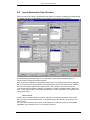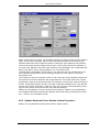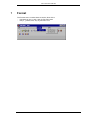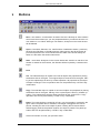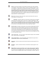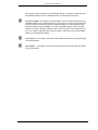
1
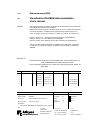
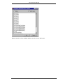
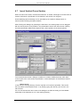
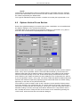
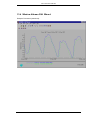
User’s Manual
KALGUI
Visualisation KALMAN data-assimilation
User’s Manual
KALGUI
Visualisation KALMAN data-assimilation
Version
Maintenance
Copyright
:
:
:
2.11, September, 2012
see www.helpdeskwater.nl/waqua
Rijkswaterstaat
Versie-geschiedenis
ve rsie
datum
JIRA
W ijz iginge n te n opz ichte van de vorige ve rsie
2.11
11-09-2012
3700
Diverse tekstuele verbeteringen
Rijkswaterstaat RIKZ
Client
Visualisation KALMAN data-assimilation
Users manual
Title
This report describes the design of a Graphical User Interface for the visualisation
of KALMAN data-assimilation simulations.
Moreover the GUI is suitable to visualise results of any 2 or 3 dimensional Waqua
in Simona simulation, provided that the postprocessing software has run correctly. This report is the second report in a series of 3 reports. The reports are:
Abstract
Report I, version 2.10: Design/System documentation of KALMAN-GUI
Report II, version 2.10: User Manual of KALMAN-GUI
Report III, version 2.00: Appendix System Documentation of KALMAN-GUI
The GUI has been build in MATLAB 5.3 software and is applicable on Windows
as well as Linux operating systems, provided that the MATLAB 5.3 software is
available.
References
Project extension assignment contract RKZ-535a, Project KUST*HYD, reference RIKZ/OS995130 dated: 28 januari 1999
Project extension assignment nr. 22001103, Project KUST*HYD, dated: 18
april 2000
Rev.
Originator
Date
Remarks
Checked by
Approved by
0
5-11-98
1
19-11-98
final vrs 1.0
1.0
2
27-04-99
draft vrs 1.01
P. van den Bosch
3
20-05-99
final vrs 1.01
P. van den Bosch
4
07-06-00
draft vrs 1.10
P. van den Bosch
Document Control
Contents
Status
Report number:
A628R2r4
text pages:
41
preliminary
Keyw ords:
Waqua, Graphical User Interfaces
tables:
0
draft
figures:
18
final
appendices:
0
Project number:
A307, A414, A628
File location:
Q:\trunk\src\matlab\kalgui\doc\usedoc\kalgui_users_manual.
doc
visiting address
e-mail
PO Box 248
De Deel 21, Emmeloord
[email protected]
8300 AE, Emmeloord
tel : +31 527 62 09 09
internet
The Netherlands
fax: +31 527 61 00 20
http://w w w .alkyon.nl
postal address
User’s Manual KALMAN GUI
Executive’s summary
This report describes the design of a graphical user interface (GUI) for the visualisation of
Kalman data assimilation simulations which are made with the WAQUA in SIMONA software.
The GUI has been build in MATLAB 5.3 software and is applicable under Windows and
Linux operating systems on PC’s as well as on workstations, as long as the MATLAB software is available.
Moreover the GUI is suitable to visualise results of any 2 or 3 dimensional Waqua in Simona
simulation, provided that the postprocessing software has run correctly. This report is the
second report in a series of 3 reports. The reports are:
Report I, version 2.00:
Report II, version 2.10:
Report III, version 2.10:
Design of KALMAN-GUI
User Manual of KALMAN-GUI
System Documentation of KALMAN-GUI
No knowledge of MATLAB is necessary to use the GUI. The GUI has a windows look and feel,
which is completely in agreement with the look and feel of most of the windows based software. The intuition of the user guides him through the user interface. On line help (via a
common Internet browser) is available for all parts of the user interface. Exporting figures or
plots in postscript, or copying plots or figures towards the clipboard for reporting purposes
in Word documents is as easy as any other copy action under windows.
In the design philosophy care has been taken for a quick and efficient use of data. Automatic scaling has been used almost everywhere, for quick handling, however if the user requires so, he has the options to use his own scale options. Mouse pointing, dragging, copying and saving of plots as well as scaling and automatic recognition of data files, belong to
the possibilities. For easy positioning a snap to grid option was added.
The design philosophy behind the GUI is framed in a data-structure, which is following as
much as possible the MATLAB structure. At the same time as less as possible use was made
of the global variable space in the MATLAB data structure. This opens the possibilities to use
the MATLAB command language independent of the Kalman GUI or within the Kalman GUI, as
required by the user.
There is also a wizard version of the Kalman GUI available.
Version 2.11, September, 2012
i
User’s Manual KALMAN GUI
Contents
1 Introduction.......................................................................................................................1
1.1 Background
1
2 File Organisation ..............................................................................................................2
2.1 New
2
2.2 Close
2
2.3 Open
2
2.4 Save and Save As
2
2.5 Export
2
3 Edit Graphic Objects.........................................................................................................5
3.1 Copy
5
3.2 Cut
5
3.3 Paste
5
3.4 Delete
5
3.5 Clipboard
6
3.6 Properties
6
3.6.1
3.6.2
3.6.3
6
6
7
Line Properties
Arrow properties
Color Selection
4 Insert Objects ...................................................................................................................8
4.1 Insert Box
8
4.2 Insert Line
8
4.3 Insert Arrow
8
4.4 Insert Text
9
4.5 Insert Timeseries
9
4.5.1 Options Timeseries
4.6 Insert Horizontal Cross Section
11
12
4.6.1 Options Horizontal Cross Section
4.6.2 Options Horizontal Cross Section: button Properties…
4.7 Insert Vertical Cross Section
14
15
17
4.8 Options Vertical Cross Section
19
4.8.1
Create Vertical Cross Section
20
5 Tools ..............................................................................................................................22
6 View................................................................................................................................23
6.1 Select Objects
23
7 Format............................................................................................................................24
8 Options...........................................................................................................................25
9 Buttons ...........................................................................................................................26
10 Pop-up menus ................................................................................................................29
Version 2.11, September, 2012
ii
User’s Manual KALMAN GUI
11 Installation notes.............................................................................................................32
11.1 PC environment
32
11.2 Linux environment
32
12 Configuration file ............................................................................................................33
12.1 Datatypes
33
12.2 Linestyles
34
12.3 Arrow shapes
34
12.4 Color definition
34
12.5 Drawing options
35
12.6 Timeseries
35
13 KALMAN – GUI: WIZARD ................................................................................................37
13.1 Introduction
37
13.2 Dialog window KALMAN – GUI: Wizard
37
13.3 Dialog window Wizard: data - type
38
13.4 Window Kalman GUI: Wizard
39
Version 2.11, September, 2012
iii
User’s Manual KALMAN GUI
1
Introduction
1.1
Background
Within the scope of the project KUST*HYD, at the RIKZ a general purpose algorithm for
online data assimilation has been developed. This development the so-called Kalman-filter
is a state of the art method to combine model results and measurements to an optimal prediction methodology. At this moment there is no user-friendly tool available to visualise the
results of a series of simulations which is made with the Kalman data-assimilation software,
which was build on top of the WAQUA in SIMONA flow simulation software.
For a good determination of the efficiency of the Kalman filter, RIKZ needed a visualisation
tool. This was the reason for Rijkswaterstaat RIKZ to write a request for proposal for the design and construction of a Graphical User Interface (GUI) for the visualisation of Kalman filter data-assimilation simulations.
On 24 March 1998, Rijkswaterstaat RIKZ in The Hague, requested Alkyon Hydraulic Consultancy and Research at Emmeloord, by a letter (in Dutch) with reference RIKZ/OS985460 to
submit such a proposal.
Such a final proposal (in Dutch) was submitted to Rijkswaterstaat RIKZ on May 18, 1998 with
reference A307le02.
The assignment was given on 18 May, 1998 by letter with reference RIKZ/OS985830. The
contract was signed on May 26, 1998.
The assignment resulted in version 1.0 of the KalGui software and the documentation which
was delivered on 19 November, 1998.
On 23 November 1998, Rijkswaterstaat RIKZ in The Hague, requested Alkyon Hydraulic
Consultancy and Research at Emmeloord, by a letter (in Dutch) with reference
RIKZ/OS987164 to submit a proposal for an extension of contract RKZ-535.
The proposal (in Dutch) for this extension was submitted to Rijkswaterstaat RIKZ on December 15, 1998 with reference A414le01.
The extension of the contract was awarded on 28 January, 1999 by letter with reference
RIKZ/OS995130. The contract, RKZ-535A was signed on March 2, 1999.
The assignment resulted in version 1.01 of the KalGui software and the documentation.
On 9 March 2000, Rijkswaterstaat RIKZ in The Hague, requested Alkyon Hydraulic Consultancy and Research at Emmeloord, by a letter (in Dutch) with reference RIKZ/OS2000/05426 to submit a proposal for an extension of the KalGui software.
The proposal (in Dutch) for this extension was submitted to Rijkswaterstaat RIKZ on March
29, 2000 with reference A628le01.
The assignment was given on 18 April, 2000 by letter with assignment nr. 22001103.
The assignment resulted in version 1.10 of the KalGui software and the documentation.
This version (2.10) has been made by Simtech. Version 2.10 has the functionality of both
the Alkyon version (1.10) and the Simtech version.
This report gives the Users Manual of the KALMAN GUI, which is also on-line available via a
WEB-browser.
Version 2.11, September 2012
1
User’s Manual KALMAN GUI
2
File Organisation
The File menu consists of the menu items New and Close for starting and finishing a visualisation session. The Export menu item gives the possibility of exporting the figure contents to
file in a specified graphic format. With the Open, Save and Save As items a session can be
load from and saved to a file. Print and Print Set-up facilitate printing of the current drawing.
2.1
New
A new session is started. If there is already an active session which hasn't been saved yet,
you are prompted whether you want to save the current session or not. When starting a new
session, all objects on the main window will be deleted. The Edit and Insert menus are enabled.
2.2
Close
All objects at the window are deleted. If the current session hasn't been saved yet, you are
prompted whether you want to save the current session or not.
2.3
Open
Selection of a .mat file with a visualisation session, previously saved by the File/Save or
File/Save As item. After opening the file all saved objects are replaced in the current window
and the state of the GUI is exactly the same as it was when the session was saved.
2.4
Save and Save As
All objects in the current window are saved to a .mat file. If the session is stored for the first
time (Save) or in case of Save As, the filename will be inquired by a selection dialogue.
2.5
Export
The objects in the presentation window can be exported to several graphical formats. Moreover a number of times and stations can be defined for which the export has to be done.
The selection of times and stations is done by the Export dialogue, which is activated by the
File/Export menu item.
Version 2.11, September 2012
2
User’s Manual KALMAN GUI
This dialogue shows a list of timelevels, which are available for all time dependent objects in
the figure and also a list of stations, available for all station dependent objects. Both the
Times list and the Stations list allows multiple selections. The graphic format can be
choosen by the radio buttons. When the 'OK' button is clicked, the objects in the figure
which are time or station dependent are redrawn for each of the selected times and stations
while the resulting figure for each of the selections is exported to a file, in the format as
specified. The procedure of redrawing and exporting the figure is given below by means of
some pseudo code.
for all selected times do
for all selected stations do
set time to selected time for all time dependent objects
set station to selected station for all station dependent objects
redraw all objects
export figure to file
end
end
The procedure above holds for all objects withor vertical cross sections and timeseries.
Timeseries objects however may have more than one series while each of them belongs to
a different station. In this situation the initial relation between the station index nrs. is used
for the export function (see example).
Example:
Initial situation:
list of 10 available stations
horizontal cross section with station nr. 1
timeseries with series (prediction and measurement) for stations 1 and 2
Version 2.11, September 2012
3
User’s Manual KALMAN GUI
Selected stations:
1, 4 and 6
Selected times:
none
Created figures:
figure 1: map for station 1 and timeseries with series for station 1 and 2
figure 2: map for station 4 and timeseries with series for station 4 and 5
figure 3: map for station 6 and timeseries with series for station 6 and 7
Version 2.11, September 2012
4
User’s Manual KALMAN GUI
3
Edit Graphic Objects
Graphic objects can be selected by clicking them with the left mouse button. Line and patch
objects are selected when the mouse is clicked just at the line or the patch. Line objects are
the objects created by Insert/line and Insert/box. An axes object is selected when the mouse
is clicked inside the definition area of the axes. Axes objects are the visualisations (cross
sections and timeseries), and the logo. More than one object can be selected by pressing
SHIFT key while selecting the objects, or by clicking with the middle mouse button instead of
the left one.
When an object is selected, it is marked as selected. Selected objects can be resized interactively by clicking the mouse at one of the corners, or endpoints when it is a line object,
and dragging it to its new size.
Copy, move and delete operations on selected objects are done by the Edit menu items
Copy, Cut, Paste and Delete. Copy, Cut and Paste always operate on one object, even if
multiple objects are selected, while Delete operates on all selected objects.
With the properties item it is possible to change the properties of a selected object.
Finally the contents of a figure can be copied to the windows clipboard by the Figure>Clipboard item.
3.1
Copy
The selected object is copied to an internal object and prepared for placing somewhere else
in the figure. Placing of the copied object is done by a Paste operation. The copied object
has the same properties as the original one. A copy operation also can be performed by a
CTRL-C key combination.
3.2
Cut
The selected object is copied to an internal object and prepared for placing somewhere else
in the figure. The original object is removed from the figure. Placing of the copied object is
done by a Paste operation. All properties of the object are kept unchanged. The cut operation also can be performed by a CTRL-X key combination.
3.3
Paste
The internal object, created by a Copy or a Cut operation, is placed in the figure. When the
paste item is activated, a rectangle is dragged at the mouse pointer, showing the size of the
object to paste. Clicking the left mouse button while dragging, defines the position at which
the object is pasted. The paste operation also can be performed by a CTRL-V key combination.
3.4
Delete
The selected object is removed from the figure. The delete operation also can be performed
by a CTRL-D key combination.
Version 2.11, September 2012
5
User’s Manual KALMAN GUI
3.5
Clipboard
The contents of the complete figure is copied to the windows clipboard. Copying from the
clipboard to other windows-based applications can be done by a CTRL-V operation.
3.6
Properties
A properties dialogue is launched in order to change the properties of the selected object.
The layout of the property dialogue depends on the type of the selected object. Objects of
which properties can be changed are a Line, Text, Arrow, TimeSeries, Horizontal Cross section and Vertical Cross section. A box is treated as a line object. Text properties are
changed with the same dialogue as used by the creation of text.
3.6.1 Line Properties
Line properties can be changed with the dialogue as shown below.
Color, Linestyle and Linewidth can be set by the controls of this dialogue. The Color button
pops-up the standard color selection dialogue. The lists of linestyles is defined in the configuration file kalguidef.m.
3.6.2 Arrow properties
Arrow properties can be changed by the 'Arrow definition' dialogue as shown below. This
dialogue has controls for specifying the length, direction and color of the arrow, width of the
arrow base and the shape of the arrow head.
The 'Angle' item, which defines the direction of the arrow, must be defined in degrees with
respect to the bottom line of the figure. The length of the arrow must be given in centimetres. The shape listbutton contains the names of a number of predefined arrow shapes
which are specified in the configuration file. This list of predefined arrow shapes easily can
Version 2.11, September 2012
6
User’s Manual KALMAN GUI
be extended. The 'Color' button pops-up the standard color selection dialogue for selection
of the color of the arrow.
3.6.3 Color Selection
Colors of graphical objects can be selected by the standard color selection dialogue.
Basic colors are selected by clicking one of the colored areas at the left side of the dialogue. Custom colors can be defined by specifying the RGB values of the desired color, at
the right side of this dialogue. The RGB values of a color are three integer values in the
range [0-255] specifying the intensity of Red, Green and Blue in the color. Defined custom
colors can be added to the basic colors and they are stored as Matlab user-defined configuration variables, so they are available in other Matlab sessions too.
Version 2.11, September 2012
7
User’s Manual KALMAN GUI
4
Insert Objects
Objects can be placed in the presentation area of a figure. Objects which can be inserted
are the items of the Graphic sub-menu, Box, Line, Text and Arrow. Also the visualisations
defined by 'TimeSeries', 'Horizontal Cross Section' and 'Vertical Cross Section' are objects
which can be inserted in the presentation area.
After selecting the object to insert, the position of the object in the figure is controlled by
mouse operations.
4.1
Insert Box
After selecting the menu item 'Insert/Graphic/Box' the position of one of the corners of the
box, in the figure is defined by pressing the left mouse button. Now moving the mouse while
pressing the left button, will show a rubberband box, with one corner fixed, while the opposite corner is moved with the mouse pointer. Releasing the mouse button, will define the opposite corner of the box and the final box will be drawn. Properties, such as color, linestyle
and linewidth of the box can be changed by selecting the box. The box is selected by clicking at one of the lines and then operate the 'Edit/Properties' menu.
4.2
Insert Line
With the menu item 'Insert/Graphic/Line', a single straight line can be inserted somewhere in
the figure. After selecting this item, the begin-point of the line is defined by the position of
the mouse pointer, when the left mouse button is pressed. Moving the mouse, while the left
button is pressed, shows a rubberband line from the begin-point to the mouse pointer. Release of the left button defines the end-point of the line and at that moment, the final line will
be drawn. Properties, such as color, linestyle and linewidth of the line can be changed by
selecting the line and then operate the 'Edit/Properties' menu.
4.3
Insert Arrow
An arrow can be inserted somewhere in the figure by clicking the menu item 'Insert/Graphic/Line'. After selecting this item, the begin-point of the arrow is defined by the
position of the mouse pointer, when the left mouse button is pressed. Moving the mouse,
while the left button is pressed, shows a rubberband line from the begin-point to the mouse
pointer. Release of the left button defines the end-point of the arrow and at that moment,
the arrow will be drawn. Properties, such as color, shape, angle, length and width of the arrow can be changed by selecting the line and then operate the 'Edit/Properties' menu.
Version 2.11, September 2012
8
User’s Manual KALMAN GUI
4.4
Insert Text
Text can be inserted everywhere in the figure by means of the menu item 'Insert/Graphic/Text'. Clicking this item is launches a text definition dialogue for specification of
the text properties.
The rotation angle must be defined in degrees with respect to the bottom line of the figure.
Color and font can be specified by the corresponding buttons which creates the standard
color- and font selection dialogues. After finishing this dialogue by pressing the OK button
the text object can be dragged with the mouse pointer to its final position. Clicking the left
mouse button will draw the text at the current position of the mouse pointer.
4.5
Insert Timeseries
Timeseries can be selected and drawn by means of the dialogue as shown below. This dialogue is activated by the 'Insert/TimeSeries' menu item.
Some detailed graphical settings can be specified by the 'Options' dialogue which is
launched after pressing the Options button.
After finishing this dialogue by pressing the OK button, the drawing object can be dragged
with the mouse pointer to its position in the presentation area of the main window. Clicking
the left mouse button will draw the object at the current position of the mouse pointer.
The 'TimeSeries' dialogue consists of a number of different areas, each area covers a part
of the timeseries specification. A short description of the different areas is given below.
Select run-id
In this area the working directory and the required run-id must be specified. This can be
done by means of the Browse button, or by directly typing the directory and run-id in the
edit controls.
If a run-id is selected the other areas of the dialogue are filled according to the available
model files of the selected run-id, in the working directory.
Version 2.11, September 2012
9
User’s Manual KALMAN GUI
Type of Data
In this listbox you can specify the datatype you want to select for presentation. The listbox
contains all datatypes which are available for the currently selected run-id.
Remark: direction means the degrees of the compass angle = angle with respect to the
North (range: 0-360 degrees). Wind direction is the direction the wind is blowing from.
Source
With the radiobuttons in the source area, you can select whether you want to present 'Predicted' or 'Measured' results.
Station
The Station listbutton shows the available locations.
Linetype / Color
With these two listbuttons it is possible to specify the linestyle and color of the current timeseries.
Markertype / Size
With these two listbuttons it is possible to specify the marker type and size of the current
timeseries.
Current Selection
This listbox shows the current selected timeseries which will be presented in one graph.
Pressing the 'Add' button, will add the timeseries defined by the current settings of the 'Runid', 'Type of Data', 'Source', 'Station', 'LineType' and 'Color' controls, to the current selec-
Version 2.11, September 2012
10
User’s Manual KALMAN GUI
tion. Pressing the 'Delete' button will remove the selected item in the 'Current Selection' box
from the current selection. Pressing the 'Modify' button, will re-define the selected item in
the 'Current Selection' box, by adding the current specified settings to it.
Time
The edit controls in this area specify the start and endtime of the graph to plot. By default,
the values in these controls specifies the overlapping time interval which is defined by the
available data of the items from the current selection list. However it is possible to edit the
values in these controls to specify a user-defined interval. Because the values are automatically re-defined by each new selection, it is recommended to specify the user-defined
interval just before finishing this dialogue.
Layout
Two titles can be specified in this area. Default titles are generated during the selection
process. Non-default titles can be entered in the edit controls, however at each new selection it will be replaced by the default texts.
The 'Legend' radiobuttons specify whether a legend is presented or not.
4.5.1 Options Timeseries
Some graphical settings can be changed by the 'TimeSeries Options' dialogue.
Automatic or Manual scaling can be defined for the Y-axis. If manual scaling is chosen, then
the minimum and maximum values for the y-axis have to be specified.
A text label can be given to draw along the Y-axis.
For the X-axis also automatic or manual scaling can be defined. If manual scaling is chosen,
then you have to specify the day and hour interval at which a label has to be placed. Also
the number of tickmarks between two labels have to be given.
With 'Show gridlines' it is possible to draw gridlines instead of tickmarks.
Default settings for these options are given in the configuration file.
Version 2.11, September 2012
11
User’s Manual KALMAN GUI
4.6
Insert Horizontal Cross Section
When the menu item 'Insert / Horizontal Cross Section' is clicked, a dialogue as shown below
is created, with which a specification of the desired cross section can be given.
Some detailed graphical settings can be specified by the 'Options' dialogue which is
launched after pressing the Options button.
After finishing this dialogue by pressing the OK button, the drawing object can be dragged
with the mouse pointer to its position in the presentation area of the main window. Clicking
the left mouse button will draw the object at the current position of the mouse pointer.
The 'Horizontal Cross Section' dialogue consists of a number of different areas, while each
area covers a part of the cross section specification. A short description of the different areas is given below.
Select run-id
In this area the working directory and the required run-id must be specified. This can be
done by means of the Browse button, or by directly typing the directory and run-id in the
edit controls.
If a run-id is selected the other areas of the dialogue are filled according to the available
modelfiles of the selected run-id, in the working directory.
Version 2.11, September 2012
12
User’s Manual KALMAN GUI
Location
With the controls in this area you can specify whether the cross section is located at one of
the layers of the model, or if it is located at a specified fixed depth. In the latter case values
will be interpolated between the layers of the model and therefore files of the desired quantity have to be available for all layers of the model.
Fixed depth's can be defined with respect to the NAP level or with respect to the waterlevel.
If the current model, defined by the selected run-id, is a two dimensional model, only the
available layer can be selected, by default this will be layer zero.
Current Selection
This listbox shows the current selected horizontal cross sections which will be presented in
one graph. By pressing the 'Add' button the horizontal cross sections, defined by the current settings of the 'Run-id', 'Location', 'Data (scalar and/or vector)', 'Source' and 'Time', will
be added to the current selection. By pressing the 'Delete' button the selected item in the
'Current Selection' box will be removed from the current selection. By pressing the 'Modify'
button the selected item in the 'Current Selection' box will be re-defined, by adding the current specified settings to it.
Remark: only the first item can be modified.
The settings for 'Location', 'Data (scalar and/or vector)', 'Source' and 'Time' of the other
horizontal cross sections should correspond to the first horizontal cross section. After modification of the first horizontal cross section all other horizontal cross sections will be modified
according to the settings of the first item.
Dry point correction
Dry point correction gives you the possibility to identify/leave out points that are dry. With
scalar data, dry points have a special, user specified color. If checkbox Vector is checked,
then vectors belonging to cells that are dry are left out.
Dry point correction is activated by checking the checkbox. There are separate checkboxes
for scalar and vector data. Dry point correction has only effect with time-dependant maps,
because dry points are time dependant. Of course dry point information must be available
to show them.
Scalar Data
The controls in this area enable you to specify a two dimensional filled contour plot of a scalar quantity.
With the 'Show - Yes' and 'Show - No' radiobuttons you can specify whether you want to plot
a scalar quantity or not.
The 'Type of Data' listbox contains the names of the available quantities at the selected
layer.
Remark: direction means the degrees of the compass angle = angle with respect to the
North (range: 0-360 degrees). Wind direction is the direction the wind is blowing from.
The radiobuttons in the 'Source' frame can be used to select one of the following sources:
Harmonic Analysis
- the effect of a harmonic component
Prediction
- map data
Gain
- gain of a KALMAN station
Standard Deviation
- standard deviation of the KALMAN simulations
Mode
- a KALMAN mode
Choice of ‘Harmonic Analysis’ requires a selection of the harmonic component of which you
want to study the effect.
Choices of 'Gain' and 'Mode' require a detailed selection of the KALMAN station and the
KALMAN mode, respectively, which can be done by means of the listbuttons 'Stations' and
'Modes'.
Version 2.11, September 2012
13
User’s Manual KALMAN GUI
If for a certain source no files are available (related to the selected datatype and location),
than the corresponding radiobutton will be disabled.
Vector Data
The controls in this area enable you to specify a vector plot of a two-dimensional quantity.
With the 'Show - Yes' and 'Show - No' radiobuttons you can specify whether you want to plot
vectors or not.
The other controls in this area, like 'Type of Data', 'Sources', 'Stations' and 'Modes' have
the same functionality as described in the 'Scalar Data' area, except they now refer to the
available vector quantities.
Time
The 'Time' listbox contains a list of available dates and times for the current selection made
in the 'Location', 'Scalar Data' and 'Vector Data' area.
Because the list of times presented here is the collection of the available times of the selection of 'Scalar Data' and the selection of 'Vector Data', it is not necessary that both the
scalar selection and the vector selection are available for all presented times. The availability of the required files is checked when the 'OK' button is pressed.
Layout
Three titles can be specified in this area. Default titles are generated during the selection
process. Non-default titles can be entered in the edit controls, however at each new selection it will be replaced by the default texts.
The 'Legend' radiobuttons specify whether a colorbar at a scalar plot is presented or not.
4.6.1 Options Horizontal Cross Section
Some of the graphical settings can be modified with the 'Options' dialogue of the 'Horizontal
Cross Section'.
The Scalar data can be presented by an IsoPatch drawing, by contourlines, or by both of
them when the contourlines are superimposed on the isopatches.
Version 2.11, September 2012
14
User’s Manual KALMAN GUI
When contourlines are chosen, it is possible to specify the levels at which the lines must be
drawn. If they are not specified, then the class boundaries defined by the minimum and
maximum data value and the default number of classes are used. Minimum and maximum
values of the scalar quantity always must be given. These values specify the extremes of
the color scale. Different color scales are defined for each datatype in the configuration file.
Axes can be drawn, with or without gridlines, in a user-defined color.
Landboundaries, if available, can be drawn or not, while the color can be selected by the
color selection dialogue which is launched by pressing the 'Color' button in the 'Landboundaries' area.
The number of vectors to be drawn in both X- and Y-direction can be specified. Default values for these vectors are defined in the configuration file. The length scale of the vectors,
specifying the value that corresponds with one centimetre, can be given if manual scaling is
chosen. If automatic scaling is chosen, the length scale will be determined in a way that the
vectors don't overlap each other. Finally the color of the vectors can be selected by pressing the 'Color' button, that launches the color selection dialogue.
Stations can be plotted or not in the horizontal cross section. Stations can be selected by
the Properties Horizontal Cross Section dialogue, that is launched by pressing the 'Properties…' button in the 'Plot stations' area.
4.6.2 Options Horizontal Cross Section: button Properties…
Stations can be plotted as markers and/or with the station names.
Version 2.11, September 2012
15
User’s Manual KALMAN GUI
Make a selection of the available stations and click on the OK button.
Version 2.11, September 2012
16
User’s Manual KALMAN GUI
4.7
Insert Vertical Cross Section
When the menu item 'Insert / Vertical Cross Section' is clicked, a dialogue as shown below is
created, with which a specification of the desired cross section can be given.
Some detailed graphical settings can be specified by the 'Options' dialogue which is
launched after pressing the Options button.
After finishing this dialogue by pressing the OK button, the drawing object can be dragged
with the mouse pointer to its position in the presentation area of the main window. Clicking
the left mouse button will draw the object at the current position of the mouse pointer.
The 'Vertical Cross Section' dialogue consists of a number of different areas, each area
covers a part of the cross section specification. A short description of the different areas is
given below.
Select run-id
In this area the working directory and the required run-id must be specified. This can be
done by means of the Browse button, or by directly typing the directory and run-id in the
edit controls.
If a run-id is selected the other areas of the dialogue are filled according to the available
model files of the selected run-id, in the working directory.
Version 2.11, September 2012
17
User’s Manual KALMAN GUI
Location
With the controls in this area you can specify the location of the cross section, you want to
visualise. Already defined cross sections are presented in the 'Cross section' listbox. A
cross section can be defined by clicking the 'Create Cross Section' button, which enables
you to define a cross section somewhere in the computational grid.
The quantities to visualise are interpolated to the cross section and therefore datafiles of all
layers and all layer interface files need to be present. If one or more files are not available,
the corresponding quantity can't be visualised.
Scalar Data
The controls in this area enable you to specify a two dimensional filled contour plot of a scalar quantity.
With the 'Show - Yes' and 'Show - No' radiobuttons you can specify whether you want to plot
a scalar quantity or not.
The 'Type of Data' listbox contains the names of the available quantities at the selected location. The radiobuttons in the 'Source' frame can be used to select one of the following
sources:
Prediction
Gain
Standard Deviation
Mode
- map data
- gain of a KALMAN station
- standard deviation of the KALMAN simulations
- a KALMAN mode
Choices of 'Gain' and 'Mode' require a detailed selection of the KALMAN station and the
KALMAN mode, respectively, which can be done by means of the listbuttons 'Stations' and
'Modes'.
If for a certain source no files are available (related to the selected datatype and location)
than the corresponding radiobutton will be disabled.
Vector Data
The controls in this area enable you to specify a vector plot of a two-dimensional quantity.
With the 'Show - Yes' and 'Show - No' radiobuttons you can specify whether you want to plot
vectors or not.
The other controls in this area, like 'Type of Data', 'Sources', 'Stations' and 'Modes' have
the same functionality as described in the 'Scalar Data' area, except they now refer to the
available vector quantities.
Time
The 'Time' listbox contains a list of available dates and times for the current selection made
in the 'Location', 'Scalar Data' and 'Vector Data' area.
Because the list of times presented here is the collection of the available times of the selection of 'Scalar Data' and the selection of 'Vector Data', it is not necessary that both the scalar selection and the vector selection are available for all presented times. The availability of
the required files is checked when the 'OK' button is pressed.
Version 2.11, September 2012
18
User’s Manual KALMAN GUI
Layout
Three titles can be specified in this area. Default titles are generated during the selection
process. Non-default titles can be entered in the edit controls, however at each new selection it will be replaced by the default texts.
The 'Legend' radiobuttons specify whether a colorbar at a scalar plot is presented or not.
4.8
Options Vertical Cross Section
Some of the graphical settings of a vertical cross section visualisation can be modified with
the 'Options' dialogue of the 'Vertical Cross Section'.
The Scalar data can be presented by an isopatch drawing, by contourlines, or by both of
them when the contourlines are superimposed on the isopatches.
When contourlines are chosen, it is possible to specify the levels at which the lines must be
drawn. If they are not specified, then the class boundaries defined by the minimum and
maximum data value and the default number of classes are used. Minimum and maximum
values of the scalar quantity can be set. These values specify the extremes of the color
scale. Different color scales are defined for each datatype in the configuration file. Axis limits can be specified for both x- and y-axis. The values -9999 and 9999 are default values for
minimum and maximum respectively. Specifying these values will result in a default scaling,
depending on the data, for the particular axis limit.
The number of vectors to draw in both X- and Y-direction can be specified. Default values
for this are defined in the configuration file. The length scale of the vectors, specifying the
value which corresponds with one centimetre, can be given if manual scaling was chosen. If
automatic scaling is chosen, the length scale will be determined in a way that the vectors
don't overlap each other. Finally the color of the vectors can be selected by pressing the
'Color' button, which launches the color selection dialogue.
Version 2.11, September 2012
19
User’s Manual KALMAN GUI
4.8.1 Create Vertical Cross Section
A vertical cross section is defined by a polygon in the horizontal plane. This polygon can be
define by clicking the lines in the 'Create Cross Section' window.
This window shows the computational grid with the landboundaries, if available. The cross
section can be defined by clicking its position in this window, with the left mouse button. After clicking the last point of a cross section, you should click the right mouse button, to end
the definition process.
When a cross section is defined it should be saved to file, which can be done by means of
the 'Save' button. Before the actual save, you are prompted for a logical name for the current cross section. The name specified here will be presented in the 'Cross Section' listbox
of the 'Vertical Cross Section' dialogue (without prefix ‘runid’_vcs_ ).
The current cross section can be removed from the window by pressing the 'Remove' button.
The 'Load' button enables you to load and visualise already defined and saved cross sections.
Speedbuttons:
Remove = removes the current vertical cross section.
Version 2.11, September 2012
20
User’s Manual KALMAN GUI
Load = loads and visualises already defined and saved vertical cross sections.
Save = saves the vertical cross section.
Zoom in = Activate the zoom function by clicking the Zoom In button in the toolbar.
Click on the area of the axes where you want to zoom in, or drag the cursor to
draw a box around the area where you want to zoom in. MATLAB redraws the
axes, zooming in on the area you specified. To further magnify the area, click repeatedly in the axes or draw additional boxes in the axes. To end zoom in mode,
click the Zoom In button.
Zoom out = To zoom out from an axes, click the Zoom Out button on the toolbar
and then click on an area of the axes where you want to zoom out. To end zoom
out mode, click the Zoom Out button.
Depth = To show the depth, click the ‘Depth yes/no’ button on the toolbar. To hide
the depth, click this button again.
Grid = To show the grid, click the ‘Grid yes/no’ button on the toolbar. To hide the
grid, click this button again.
Version 2.11, September 2012
21
User’s Manual KALMAN GUI
5
Tools
With the Tools menu it is possible to step through the available list of times or stations of the
selected objects. The items of the Tools menu are shown in the figure below.
The menu items 'Next time' and 'Previous time' can be used to step through the available
time levels of the selected objects. If more than one object is selected then 'Next time' selects the next available time level for each selected object. 'Next time' steps forward in the
list of available times, while 'Previous times' steps one item backward in this list. When the
last time level is reached, 'Next time' doesn't have any effect for the particular object. The
same yields for 'Previous time' when the current time level of an object is the first one in the
list. The 'Select Time' item comes with a list of time levels, available for all selected objects.
The items 'Next station', 'Previous station', and 'Select station' have the same functionality
as the corresponding 'Time' items, but now they operate on the list of available stations for
the selected objects.
The 'Time' items will be enabled when one or more of the selected objects are a 'Horizontal
Cross Section' or a 'Vertical Cross Section'. The 'Station' items will be enabled when one or
more of the selected objects are a 'Time Series' or a 'Horizontal Cross Section' or 'Vertical
Cross Section' with a KALMAN station selected.
Version 2.11, September 2012
22
User’s Manual KALMAN GUI
6
View
The View menu has the two Zoom items, 'Zoom In' and 'Zoom Out'. The Zoom operation is
only defined for objects of the type 'Horizontal Cross Sections'. After clicking the 'Zoom In'
item it is possible to define a zooming rectangle in a viewport with a 'Horizontal Cross Section' presentation. A zooming rectangle is defined by a rubberband box who's left below corner is defined by the mouse position when the left button is clicked, while the right upper
corner is defined by the mouse position when the button is released. Releasing the mouse
button will automatically redraw the zoomed area. The zoom operation operates on all selected objects. If more than one object is selected, the defined zooming rectangle operates
on all selected objects.
Clicking the 'Zoom Out' item resets the axis limits of all current selected objects to its original
extent.
6.1
Select Objects
Objects are selected by clicking the left mouse button, when the mouse pointer is on the object. When an object is selected, small black boxes are drawn at the corners of the object,
so it is easy to distinguish between selected and non-selected objects. In the figure below
the horizontal cross section and the line are selected, while the timeseries isn't.
More than one object can be selected by pressing SHIFT key while selecting the objects, or
by clicking with the middle mouse button instead of the left one. Objects are deselected
when a mouse button is clicked while the mouse position in not on the object.
Version 2.11, September 2012
23
User’s Manual KALMAN GUI
7
Format
The Format menu contains items to set the fonts of the:
- tick labels on the x- and y-axis: by Set Font Axes
- text (x-, y-labels, title, etc): by Set Font Text
Version 2.11, September 2012
24
User’s Manual KALMAN GUI
8
Options
The Options menu has items to facilitate the placing of objects. In the default situation objects can be placed everywhere in the presentation area of the figure. However when there
are multiple objects in the area, it may be necessary that they are outlined to a certain line.
For this reason there is a 'Snap to Grid' option, which forces that objects origins are placed
in gridpoints. This rectangular grid can be displayed by the 'Display Grid' option. The size of
the grid is defined in pixels and is defined by the 'Set Gridspacing' option.
Version 2.11, September 2012
25
User’s Manual KALMAN GUI
9
Buttons
New = new session. A new session is started. If there is already an active session
which hasn't been saved yet, you are prompted whether you want to save the current session or not. When starting a new session, all objects on the main window
will be deleted.
Open = load data. Selection of a .mat file with a visualisation session, previously
saved by the File/Save or File/Save As item. After opening the file all saved objects are replaced in the current window and the state of the GUI is exactly the
same as it was when the session was saved.
Save = save data. All objects in the current window are saved to a .mat file. If the
session is stored for the first time, the filename will be inquired by a selection dialogue.
Print
Cut. The selected object is copied to an internal object and prepared for placing
somewhere else in the figure. The original object is removed from the figure. Placing of the copied object is done by a Paste operation. All properties of the object
are kept unchanged. The cut operation also can be performed by a CTRL-X key
combination.
Copy. The selected object is copied to an internal object and prepared for placing
somewhere else in the figure. Placing of the copied object is done by a Paste operation. The copied object has the same properties as the original one. A copy
operation also can be performed by a CTRL-C key combination.
Paste. The internal object, created by a Copy or a Cut operation, is placed in the
figure. When the paste item is activated, a rectangle is dragged at the mouse
pointer, showing the size of the object to paste. Clicking the left mouse button
while dragging, defines the position at which the object is pasted. The paste operation also can be performed by a CTRL-V key combination.
Click on this button to undo your previous action.
Version 2.11, September 2012
26
User’s Manual KALMAN GUI
Zoom in. The Zoom operation is only defined for objects of the type 'Horizontal
Cross Sections'. After clicking the 'Zoom In' button it is possible to define a zooming rectangle in a viewport with a 'Horizontal Cross Section' presentation. A zooming rectangle is defined by a rubberband box who's left below corner is defined by
the mouse position when the left button is clicked, while the right upper corner is
defined by the mouse position when the button is released. Releasing the mouse
button will automatically redraw the zoomed area. The zoom operation operates on
all selected objects. If more than one object is selected, the defined zooming rectangle operates on all selected objects.
Zoom out. Clicking the 'Zoom Out' button resets the axis limits of all current selected objects to its original extent.
Next time: The button 'Next time' can be used to step through the available
time levels of the selected objects. If more than one object is selected then 'Next
time' selects the next available time level for each selected object. 'Next time' steps
forward in the list of available times. When the last time level is reached, 'Next time'
doesn't have any effect for the particular object. If no object is selected then 'Next
time' selects the next available time level for all time dependant objects.
Previous time: The button 'Previous time' can be used to step through the available time levels of the selected objects. If more than one object is selected then
'Previous time' selects the previous available time level for each selected object.
'Previous time' steps backward in the list of available times. When the first time
level is reached, 'Previous0 time' doesn't have any effect for the particular object.
If no object is selected then 'Previous time' selects the previous available time level
for all time dependant objects.
Time loop forward : ‘Time loop forward’ steps forward through the list of available
times, untill the button is pressed again.
Time loop backward : ‘Time loop backward’ steps backward through the list of
available times, untill the button is pressed again.
First time : ‘First time’ selects the first time and draws the object(s) again for the
first time.
Last time : ‘Last time’ selects the last time and draws the object(s) again for the
last time.
Next station: The button 'Next station' can be used to step through the available
stations of the selected objects. If more than one object is selected then 'Next station' selects the next available station for each selected object. 'Next station' steps
forward in the list of available stations. When the last station is reached, 'Next sta-
Version 2.11, September 2012
27
User’s Manual KALMAN GUI
tion' doesn't have any effect for the particular object. If no object is selected then
'Next station' selects the next available station for all timeseries objects.
Previous station: The button 'Previous station' can be used to step through the
available stations of the selected objects. If more than one object is selected then
'Previous station' selects the previous available station for each selected object.
'Previous station' steps backward in the list of available stations. When the last
station is reached, 'Previous station' doesn't have any effect for the particular object. If no object is selected then 'Previous station' selects the previous available
station for all timeseries objects.
First station : ‘First station’ selects the first station and draws the object(s) again
for the first station.
Last station : ‘Last station’ selects the last station and draws the object(s) again
for the last station.
Version 2.11, September 2012
28
User’s Manual KALMAN GUI
10
Pop-up menus
Pop-up menus are activated by clicking the right mouse button.
If the mouse pointer is on a object when the right-button is clicked, the pop-up menu has the
items Cut, Copy, Delete and Properties. The functionality of these items is exactly the same
as the corresponding items of the Edit menu.
Depending on the type of the selected object, the Options item will come with the 'Options
Horizontal Cross Section', 'Options Vertical Cross Section' or the 'Options Timeseries' dialogue.
If the mouse pointer is not on an object when the right-button is clicked, the pop-up menu
has the items Paste, Snap to Grid, Display Grid and Refresh.
With the Paste item, a copied or cut object can be placed in the presentation area. The Refresh item causes all objects in the presentation area to be redrawn. The 'Snap to Grid' and
the 'Display Grid' items have the same functionality as the corresponding items of the Options menu.
Two items, which are always in the pop-up menu are the 'Send to Back' and 'Bring to Front'
items. With these items the drawing sequence of the viewports can be controlled and so the
visibility of overlapping objects. This option can be used to draw arrows, lines or text objects
on top of a visualisation.
The pop-up menu of the horizontal cross section contains the extra menu-option 'Insert…'.
Version 2.11, September 2012
29
User’s Manual KALMAN GUI
The 'Insert…' menu-option opens a tab dialog window to insert vertical cross sections.
This dialog shows at the left a list of avialable vertical cross sections. With the >> button it is
possible to add one or more vertical cross section lines to the horizontal cross section plot.
It is possible to modify the line properties with the 'Edit line properties' button. All vertical
cross section lines in the horizontal cross section are shown in the list box at the right side
of this dialog. The << button removes the vertical cross section from the list at the right and
from the horizontal cross section plot.
Edit line properties:
Line properties control various aspects of the line and can be modified by the 'Edit line
properties' button.
Version 2.11, September 2012
30
User’s Manual KALMAN GUI
The line properties that can be modified are:
- line width (in points)
- line style
- marker size
- marker type
- line color
Click on the Apply button to display the result into the horizontal cross section, without
closing the dialog window.
Version 2.11, September 2012
31
User’s Manual KALMAN GUI
11
Installation notes
11.1 PC environment
Installation of the KALMAN-GUI is done with the set-up program Setup_KalGui which is on
the installation flop and CD-ROM. This set-up program installs the source files on the harddisk of your computer.
After starting this set-up program you will be prompted for
the drivename of the used installation medium (e.g. a)
the specification of the destination directory
The set-up program can adapt your personal Matlab start-up file named startup.m to add
the destination directory to the Matlab search path. If the destination directory of KALMANGUI is part of the Matlab search path, you can start the GUI from each directory, otherwise
you have to start it from the specified destination directory.
It is recommended to verify the settings in the configuration file kalguidef.m and eventually
adapt the settings to your personal preferences.
11.2 Linux environment
To install the KALMAN-GUI on an Linux system, the following actions must be done.
create a directory kalgui
create the subdirectory kalgui/help
copy all files of the kalgui\sources directory of the CD-Rom to the kalgui directory
copy all files of the kalgui\help directory of the CD-Rom to the kalgui/help directory
edit the configuration file kalguidef.m in the kalgui directory and set the path of the
installation directory. (statement instaldir = cd; )
add the installation directory to the Matlab search path by editing the path statement in
your personal start-up file. ( startup.m )
Version 2.11, September 2012
32
User’s Manual KALMAN GUI
12
Configuration file
One of the source files which is part of the KALMAN-GUI is the configuration file kalguidef.m. In this file, personal preferences are defined for:
datatypes
linestyle
arrow shape
color definition
drawing options
timeseries
12.1 Datatypes
A datatype is defined by a number of items in the drawopt.datatype struct, which define the
properties of the datatype. Adding new datatypes to the program requires that an entry in
the drawopt.datatype struct is filled. Below the list of items with the possible options is given.
name of datatype:
measurement unit:
type of presentation (scalar | vector |
time):
defined for cross section (horizontal | vertical | both):
layer dependent (yes | no):
time dependent (yes | no):
quantity is computed (yes | no):
index in drawopt.grid:
definition point in horizontal grid cell 's
(centre | corner):
definition point in vertical grid cell's (centre
| corner):
operation
(none|magnitude|direction|normal|tangenti
al):
code in filename; 1st parameter:
code in filename; 2nd parameter:
nd
code in filename; 3 parameter:
column index in datafile; timeseries only:
colormap for scalar presentation:
default range for data:
contourlevels to draw:
drawopt.datatype(1).name = 'Waterlevel';
drawopt.datatype(1).unit = 'm’;
drawopt.datatype(1).type = 'scalar';
drawopt.datatype(1).section = 'horizontal';
drawopt.datatype(1).layerdep = 'no';
drawopt.datatype(1).timedep = 'yes';
drawopt.datatype(1).computed = 'yes';
drawopt.datatype(1).defgrid = 1;
drawopt.datatype(1).hdef = 'centre';
drawopt.datatype(1).vdef = [];
drawopt.datatype(1).operation = 'none';
drawopt.datatype(1).file1 = 'sep';
drawopt.datatype(1).file2 = [];
drawopt.datatype(1).file3 = [];
drawopt.datatype(1).index = [];
drawopt.datatype(1).cmap = 'jet(16)';
drawopt.datatype(1).crange = [-.5 .5];
drawopt.datatype(1).clevels = [];
The definition grids at which the datatypes are defined are specified by the statements:
drawopt.grid(1).xfile = 'xzeta'
name of file with x-coordinates
drawopt.grid(1).yfile = 'yzeta'
name of file with y-coordinates
By default the first entry in grid must specify the grid of zeta points and the second entry
must specify the grid of the depth points. Additional grids can be specified in index three
and higher.
Version 2.11, September 2012
33
User’s Manual KALMAN GUI
12.2 Linestyles
Personal preferences with respect to linestyles can be set with the lines:
linedef(1).name='--------';
linedef(1).value='-';
where linedef(1).value specifies the Matlab code of the desired linestyle. The .name item is
a string code which is presented in the LineProperties dialogue. There is no restriction in
the number of linestyles to specify here, however the .value item must be a valid Matlab
style.
12.3 Arrow shapes
Personal preferences of arrow shapes are set with the lines:
arrowshape(1).name='normal';
arrowshape(1).head=.2;
arrowshape(1).tip_angle=60.;
arrowshape(1).base_angle=90;
The items head, tip_angle and base_angle defines the shape of the arrow head as shown
in the figure below.
The .head item defines the length of the arrow head as fraction of the total arrow length and
so it must be in the range [0. 1.].
The .name item is a string code which is presented in the shape list of the 'Arrow definition'
dialogue.
12.4 Color definition
Personal preference with respect to the choice of used colors for functions can be defined
by the coldef list:
coldef(1).name = 'blue';
coldef(1).value = '0 0 1';
Coldef.value is the so-called RGB value, which is a specification of the fractions of the Red,
Green and Blue intensity in the particular color.
Coldef.name is a string which defines a user-specific for the color.
There is no limit in the number of colors to specify in the coldef list.
Version 2.11, September 2012
34
User’s Manual KALMAN GUI
12.5 Drawing options
Drawing options are defined for:
Axes:
drawopt.showaxes = 'no';
drawopt.axes_color = 'black';
drawopt.showgrid = 'no';
drawopt.xrange = [-9999 9999];
drawopt.yrange = [-9999 9999];
The x-range and y-range items specifies the axes limits of x- and y-axes of a visualisation.
The values -9999 and 9999 presumes automatic scaling.
Landboundaries:
drawopt.landboundaries = 'yes';
drawopt.boundary_color = 'black';
Vector drawings:
drawopt.vector_scalemode = 'automatic';
drawopt.vector_scale = 1.;
drawopt.vector_color = 'blue';
drawopt.nx_vectors = 20;
drawopt.ny_vectors = 20;
The nx_vectors and ny_vectors specifies the number of vectors in the drawing in x- and ydirection respectively.
Scalar drawings:
drawopt.scalar_plottype = 'iso';
drawopt.coloured_contours = 'no';
drawopt.spec_contours = 'no';
Plottype specifies whether the drawing consists of isofaces ('iso'), contourlines ('cont') or
both of them ('both'). The coloured_contours item specifies whether the contourlines are
black, or if the current colormap should be used. If the spec_contours item is set to 'yes',
then the levels at which the contourlines must be drawn, should be specified in
"datatype().clevels".
12.6 Timeseries
For timeseries the following settings can be defined:
tmsopt.y_scalemode = 'automatic';
tmsopt.yrange = [-10. 10.];
tmsopt.ylabel = '';
tmsopt.nx_labels = 3;
tmsopt.showgrid = 'no';
tmsopt.xticks(1) = 23;
tmsopt.xticks(2) = 1;
tmsopt.xticks1to2= 5;
Version 2.11, September 2012
35
User’s Manual KALMAN GUI
The y_scalemode specifies whether the y-scale is determined automatic by minimum and
maximum of the function values, or if the specified values of yrange has to be used ('manual' mode).
The nx_labels item specifies the maximum number of date/time labels to present along the
horizontal axis.
The tmsopt.xticks(1) option defines the number of ticks between 2 time labels, if the number
of days on the x-as is less than tmsopt.xticks1to2.
The tmsopt.xticks(2) option defines the number of ticks between 2 time labels, if the number
of days on the x-as is equal or more than tmsopt.xticks1to2.
Version 2.11, September 2012
36
User’s Manual KALMAN GUI
13
KALMAN – GUI: WIZARD
13.1 Introduction
With the Wizard of the Kalman graphical user interface it is easy to visualise your data in a
few steps.
Available wizards:
- Timeseries waterlevel (predicted and observed)
- Timeseries velocity
- velocity magnitude (predicted and observed)
- velocity direction (predicted and observed)
- Timeseries salinity (predicted and observed)
- Map waterlevel (scalar) and velocity (vector)
- Map salinity (scalar) and velocity (vector)
- Map velocity magnitude (scalar) and velocity (vector)
13.2 Dialog window KALMAN – GUI: Wizard
Select run-id
In this area the working directory and the required run-id must be specified. This can be
done by means of the Modify… button.
Kalman GUI
With the radiobuttons in this area, you can select whether to start the ‘wizard’ Kalman
graphical user interface or the ‘normal’ Kalman graphical user interface.
Version 2.11, September 2012
37
User’s Manual KALMAN GUI
13.3 Dialog window Wizard: data - type
Timeseries (waterlevel)
Button Timeseries (waterlevel) will be enabled, if there are files available which contain
‘_wl_’ in their names.
Timeseries (velocity)
Button Timeseries (velocity) will be enabled, if there are files available which contain ‘_vel_’
in their names.
Timeseries (salinity)
Button Timeseries (salinity) will be enabled, if there are files available which contain ‘_sal_’
in their names.
Map: waterlevel and velocity
Button Map: waterlevel and velocity will be enabled, if there are files available which contain
‘_sep_’, ‘_up_’, ‘_vp_’ in their names.
Map: salinity and velocity
Button Map: salinity and velocity will be enabled, if there are files available which contain
‘_rp_’, ‘_up_’, ‘_vp_’ in their names.
Map: velocities (color and vectors)
Button Map: velocities (color and vectors) will be enabled, if there are files available which
contain ‘_up_’, ‘_vp_’ in their names.
Version 2.11, September 2012
38
User’s Manual KALMAN GUI
13.4 Window Kalman GUI: Wizard
Example Timeseries (waterlevel):
Version 2.11, September 2012
39