Download User's Guide WAQUA: General Information

User’s Guide WAQUA: General
Information
User’s Guide WAQUA: General
Information
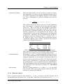
Version number
Maintenance
Copyright
:
:
:
Version 10.59, October 2013
see www.helpdeskwater.nl/waqua
Rijkswaterstaat
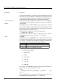
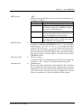
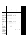
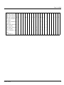
Log-sheet
Table 1: Log-Sheet
Document
version
10.27
10.28
10.29
10.30
10.31
10.32
10.33
10.34
10.35
10.36
10.37
10.38
Date
Change no
Changes with respect to previous version
P03022
P03023
13-10-2003
P03031
P03032
03-11-2003 ruwh02-b
condition on wind direction / speed not allowed at SVWP.
waqpre-input description for barriers improved.
improvements for slib3d.
layout improvements (vector arrows, integral signs, etc.)
Introduction of roughness combinations and ebb/flood roughnesses
10-11-2003 dynbar02
extension of dynamic barrier steering
14-11-2003 P03047
general check (export 2003-02)
16-02-2004 P04003
removal of (sub-)systems: waqua-oud, sispos, conidp, sdskom, sdsmap, sdspri, sdsres, sds11b
14-06-2004 DDHV01
combined horizontal and vertical domain decomposition
28-06-2004 P03043
nu-signs made more clear in Navier-Stokes equation
05-07-2004 P04008
installation of RUWH03.
13-07-2004 kalwnd01
Introduction of multiple formats in waqwnd
P03033
Description of approved weir-routines
01-09-2004
P04009
Update QAD-boundary conditions (VORtech)
DROOGV01 phase 2: new drying/flooding functionality
M04042
use defined distance (in routine "wasrv1")
M04069
correction in routine "wapttd"
P04001
extra functionality in simpar
P04012
correction in slib3d (from w04007, decay)
P05002
corrections in waqpre for droogv01 (phase 2)
P05003
collect class values (new subsystem "waqclv")
25-03-2005
P05005
correction in check on "tlsmooth" at restart
P05006
mark zero-differences in Simona-boxes (waqview)
P05008
improved barrier model (waqpro)
W04006
add maps for dynamic barriers
W04007
introduce decay in slib calculations (slib3d)
W04008
save 3D-vertical eddy diffusion coefficients on sds-file
W04013
extension of w04008 (in slib3d)
21-07-2005 DROOGV01 phase 3 – new drying/flooding functionality
Version 10.59, October 2013
i
User’s Guide WAQUA: General Information
Document version Date
10.39
03-08-2005
10.40
31-08-2005
10.41
01-11-2005
10.42
20-06-2007
Change no
B05007
M04036
P05014
P05016
W04003
W05006
M05069
M05045
M05087
M05091
W05001
W05007
C71236
10.43
10.44
10.45
10.46
10.47
10.48
10.49
10.50
10.51
28-11-2007
22-05-2007
20-06-2007
21-06-2007
05-09-2007
19-09-2007
29-11-2007
31-01-2008
17-03-2008
C71236
C66699
C71236
C71236
M321608
C74807
C71236
C77132
C80842
10.52
10.53
10.54
10.55
10.56
10.57
10.58
10.59
14-08-2009
07-09-2009
01-12-2009
15-07-2010
13-09-2010
16-05-2012
01-02-2013
16-10-2013
C91583
C81107
M385558
C3256
C3410
M3754
beheer
3964
ii
Changes with respect to previous version
updates for "class values"
triwaq-correction in routine "wascht"
correction in routine "waswcv" ("class values")
extra checks for TIME_AND_VALUES
incorporation of User’s Guide couple
roughness-codes extended: 1201-1300 to 1201-1400
introduction of GSC
backtracking in simpar
correction in coppre / coppos
extra conditions for barrier steering
reference to FAQ for template
introduction of "minvalues"
keyword CDCON, ITERACCURACY and application WAQRIV removed
removed Waqbhd
Introduced linear bottom friction model
Removed CCO-file and other obsolete functionalities
Removed program Waqriv
Corrections w.r.t. missing figures and equations
Changes w.r.t. calculation of energyloss for weirs
Removed program Waqbhd
Implementation of weirs for 3D TRIWAQ models
Merged technical documentation of WAQUA and
TRIWAQ: changed general introduction of weirs.
Introduction of barrier-barrier structures
Introduction of VILLEMONTE model for weirs
Corrected cross references for barrier figures
Conversion to Latex
Waqpan removed; uniform layout logsheet
Corrections related to conversion to Latex
Removed Appendix C, systemchart
Remove outdated OpenDA information
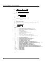
CONTENTS
Contents
1
About this manual
2
2
About SIMONA
4
2.1
Introduction . . . . . . . . . . . . . . . . . . . . . . . . . . . . . . . . . . . . . .
4
2.2
SIMONA data storage . . . . . . . . . . . . . . . . . . . . . . . . . . . . . . . .
5
2.3
The input file . . . . . . . . . . . . . . . . . . . . . . . . . . . . . . . . . . . . .
5
3
About WAQUA
3.1
3.2
Introduction to the system . . . . . . . . . . . . . . . . . . . . . . . . . . . . . .
10
3.1.1
Function of the system . . . . . . . . . . . . . . . . . . . . . . . . . . . .
10
3.1.2
Features . . . . . . . . . . . . . . . . . . . . . . . . . . . . . . . . . . . .
11
3.1.3
Modelling with WAQUA . . . . . . . . . . . . . . . . . . . . . . . . . . .
13
Geometry . . . . . . . . . . . . . . . . . . . . . . . . . . . . . . . . . . . . . . .
15
3.2.1
Computational grid . . . . . . . . . . . . . . . . . . . . . . . . . . . . . .
15
3.2.1.1
Computational grid structure . . . . . . . . . . . . . . . . . . .
15
3.2.1.2
Basic grid principle . . . . . . . . . . . . . . . . . . . . . . . .
16
3.2.1.3
Computational grid tuning and open boundaries . . . . . . . . .
18
Physical geometry . . . . . . . . . . . . . . . . . . . . . . . . . . . . . .
21
Model types . . . . . . . . . . . . . . . . . . . . . . . . . . . . . . . . . . . . . .
22
3.3.1
Rectilinear models . . . . . . . . . . . . . . . . . . . . . . . . . . . . . .
22
3.3.1.1
General . . . . . . . . . . . . . . . . . . . . . . . . . . . . . .
22
3.3.1.2
Mathematical description differential equations . . . . . . . . .
22
Curvilinear models . . . . . . . . . . . . . . . . . . . . . . . . . . . . . .
24
3.3.2.1
General . . . . . . . . . . . . . . . . . . . . . . . . . . . . . .
24
3.3.2.2
Mathematical description differential equations . . . . . . . . .
25
Spherical coordinates models . . . . . . . . . . . . . . . . . . . . . . . .
26
3.2.2
3.3
9
3.3.2
3.3.3
Version 10.59, October 2013
iii
User’s Guide WAQUA: General Information
3.3.3.1
General . . . . . . . . . . . . . . . . . . . . . . . . . . . . . .
26
3.3.3.2
Mathematical description differential equations . . . . . . . . .
26
Models using space varying wind and pressure . . . . . . . . . . . . . . .
28
General hydrodynamics . . . . . . . . . . . . . . . . . . . . . . . . . . . . . . . .
30
3.4.1
Features . . . . . . . . . . . . . . . . . . . . . . . . . . . . . . . . . . . .
30
3.4.2
Computational methods . . . . . . . . . . . . . . . . . . . . . . . . . . .
31
3.4.2.1
Time advancement of state variables . . . . . . . . . . . . . . .
31
3.4.2.2
Time integration . . . . . . . . . . . . . . . . . . . . . . . . . .
32
3.4.2.3
Forcing functions . . . . . . . . . . . . . . . . . . . . . . . . .
39
3.4.2.4
Chezy coefficient computation . . . . . . . . . . . . . . . . . .
44
3.4.2.5
Nikuradse roughness . . . . . . . . . . . . . . . . . . . . . . .
47
3.4.2.6
Roughcombination roughness . . . . . . . . . . . . . . . . . . .
52
3.4.2.7
Equation of state . . . . . . . . . . . . . . . . . . . . . . . . . .
59
3.4.2.8
Non-hydrostatic computations . . . . . . . . . . . . . . . . . . .
60
Special hydrodynamical objects . . . . . . . . . . . . . . . . . . . . . . . . . . .
61
3.5.1
Barriers and sluices . . . . . . . . . . . . . . . . . . . . . . . . . . . . . .
61
3.5.1.1
Features . . . . . . . . . . . . . . . . . . . . . . . . . . . . . .
61
3.5.1.2
Computational methods . . . . . . . . . . . . . . . . . . . . . .
69
Barrier-barrier constructions . . . . . . . . . . . . . . . . . . . . . . . . .
72
3.5.2.1
Weirs . . . . . . . . . . . . . . . . . . . . . . . . . . . . . . . .
73
3.5.2.2
Features . . . . . . . . . . . . . . . . . . . . . . . . . . . . . .
73
3.5.2.3
Computational methods . . . . . . . . . . . . . . . . . . . . . .
73
3.5.2.4
Weirs in TRIWAQ . . . . . . . . . . . . . . . . . . . . . . . . .
74
Drying and flooding (tidal flats) . . . . . . . . . . . . . . . . . . . . . . . . . . .
76
3.6.1
Features . . . . . . . . . . . . . . . . . . . . . . . . . . . . . . . . . . . .
76
3.6.2
Computational methods . . . . . . . . . . . . . . . . . . . . . . . . . . .
76
Harmonic analysis of tides . . . . . . . . . . . . . . . . . . . . . . . . . . . . . .
83
3.7.1
Features . . . . . . . . . . . . . . . . . . . . . . . . . . . . . . . . . . . .
83
3.7.2
Computational methods . . . . . . . . . . . . . . . . . . . . . . . . . . .
83
3.7.2.1
Mathematical representation of the tide . . . . . . . . . . . . . .
83
3.7.2.2
Harmonic analysis . . . . . . . . . . . . . . . . . . . . . . . . .
85
Transport of constituents . . . . . . . . . . . . . . . . . . . . . . . . . . . . . . .
87
3.8.1
87
3.3.4
3.4
3.5
3.5.2
3.6
3.7
3.8
iv
Features . . . . . . . . . . . . . . . . . . . . . . . . . . . . . . . . . . . .
CONTENTS
3.8.2
Computational methods . . . . . . . . . . . . . . . . . . . . . . . . . . .
87
3.8.2.1
Time advancement of state variables . . . . . . . . . . . . . . .
88
3.8.2.2
Forcing functions . . . . . . . . . . . . . . . . . . . . . . . . .
90
User routines . . . . . . . . . . . . . . . . . . . . . . . . . . . . . . . . . . . . .
92
3.9.1
Features . . . . . . . . . . . . . . . . . . . . . . . . . . . . . . . . . . . .
92
3.9.2
Mathematical description . . . . . . . . . . . . . . . . . . . . . . . . . . .
92
3.9.3
Data input/output . . . . . . . . . . . . . . . . . . . . . . . . . . . . . . .
93
3.9.4
Computation . . . . . . . . . . . . . . . . . . . . . . . . . . . . . . . . .
94
3.9.5
Generating procedure . . . . . . . . . . . . . . . . . . . . . . . . . . . . .
94
3.10 Data flow . . . . . . . . . . . . . . . . . . . . . . . . . . . . . . . . . . . . . . .
95
3.10.1 Input . . . . . . . . . . . . . . . . . . . . . . . . . . . . . . . . . . . . .
95
3.10.2 Output . . . . . . . . . . . . . . . . . . . . . . . . . . . . . . . . . . . .
95
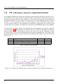
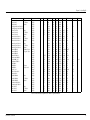
3.11 CPU and memory usage for computational models . . . . . . . . . . . . . . . . .
96
3.9
3.12 WAQUA programs . . . . . . . . . . . . . . . . . . . . . . . . . . . . . . . . . . 100
A Examples
I
A.1 Example user routine . . . . . . . . . . . . . . . . . . . . . . . . . . . . . . . . .
I
A.1.1 General . . . . . . . . . . . . . . . . . . . . . . . . . . . . . . . . . . . .
I
A.1.2 Model description . . . . . . . . . . . . . . . . . . . . . . . . . . . . . .
I
A.1.3 Input file mussel filter . . . . . . . . . . . . . . . . . . . . . . . . . . . .
II
A.1.4 Subroutine WASUST . . . . . . . . . . . . . . . . . . . . . . . . . . . . .
VI
B Definition WAQUA standard version
B.1 Standard version of May 2012 . . . . . . . . . . . . . . . . . . . . . . . . . . . .
B.1.1
SIMONA standard version subsystems . . . . . . . . . . . . . . . . . . .
XI
XI
XI
C Harmonic Constants
XII
Version 10.59, October 2013
1
User’s Guide WAQUA: General Information
Chapter 1
About this manual
The User’s Guide WAQUA contains an extensive input description of the subsystems of WAQUA.
It also describes principles and backgrounds of the WAQUA system.
WAQUA is a water movement and water quality simulation system, able to perform two-dimensional
computations. A part called TRIWAQ is incorporated for three-dimensional computations. The
system enables the user to simulate stationary as well as non-stationary flow patterns, transport of
dissolved substances, temperature distribution and sediment transport.
WAQUA is based on SIMONA, a flexible concept for the development of modelling software.
SIMONA defines an architecture for preprocessing, memory management, data storage and postprocessing. SIMONA aims for structured and controlled development of software, reducing cost for
maintenance and support.
Interested users are advised to read the chapters in section 1 dealing with SIMONA. More information is available in the SIMONA programmer’s guide.
This document is written for users, both model builders and model managers who make computer
runs for model builders.
A general introduction to the system is given in section 1 (general information) of the user’s guide
WAQUA. The other sections give more detailed descriptions of the WAQUA system.
The User’s Guide WAQUA consists of 8 sections:
section 1
2
General Information
About the manual
About SIMONA
About the WAQUA system
Chapter 1. About this manual
section 2
section 3
section 4
section 5
section 6
section 7
section 8
Quick Reference Guide
How to run the several WAQUA subsystems
User’s Guide WAQWND
Input description WAQWND
User’s Guide pre-processor WAQPRE
Input description WAQPRE
User’s Guide for Parallel WAQUA/TRIWAQ and for Domain
Decomposition
Possibilities and limitations of domain decomposition; Input description COPPRE
User’s Guide processor WAQPRO
Input description WAQPRO
User routines
User’s Guide SIMPAR
Input description SIMPAR
User’s Guide SLIB3D
Input description SLIB3D
Although the User’s Guides describing the separate subsystems make some explicit references to
section 1 (General Information), their dependencies on it are literally too numerous to mention. If a
section in a specific User’s Guide is not clear, the reader is advised to see the corresponding chapter
in General Information.
The WAQUA system as described in this User’s Guide WAQUA only deals with SIMONA based
subsystems.
Version 10.59, October 2013
3
User’s Guide WAQUA: General Information
Chapter 2
About SIMONA
In this chapter SIMONA is described. In section 2.1 the various parts of a SIMONA program system
are treated. In section 2.2 the SIMONA data storage is discussed. The input file for a SIMONA
program is described in section 2.3.
2.1
Introduction
Each SIMONA program system consists of three parts: a pre-processing part, a processing part, and
a post-processing part.
The three parts of a SIMONA program system have different functions:
pre-processing
processing
post-processing
4
In the pre-processing part all actions are taken that are needed before the actual computation can start, such as reading user input
from the input file, defining the geometry, and filling parameters,
variables and arrays with initial values. The pre-processor consists of an application independent part and an application dependent part. First the application independent part, which is provided
by SIMONA, reads the complete input file, checks its syntax and
stores the data in core. Next the application dependent part does
the interpretation of the data, checks the validity of the input, derives other initial data and writes the input to an SDS file (usually
in overwrite mode (see section 2.2)).
In the processing part the actual computation takes place. All data
needed are read from the SDS file. Results of the computation are
written to the SDS file (usually in append mode (see section 2.2)).
In the post-processing part the output is taken care of. The data
are read from the SDS file and presented in a well-ordered way in
prints and/or graphics. At this moment this part is not available.
Chapter 2. About SIMONA
2.2
SIMONA data storage
The three parts of a SIMONA program communicate with each other through a SIMONA data storage file (SDS file).
There are three types of access to an SDS file: read access, overwrite access, and append access.
These types are used to protect the integrity of the data on the SDS file.
If a program is writing in overwrite mode to an SDS file, no other program can obtain access to
that SDS file. If a program is writing in append mode to an SDS file, other programs can obtain
read access to that SDS file, but no program can obtain write access to that SDS file (neither in
overwrite mode nor in append mode). If a program is reading from an SDS file, other programs can
obtain read access to that SDS file and one program can obtain append access to that SDS file, but
no program can obtain overwrite access to that SDS file. The administration whether programs are
reading/writing to an SDS file is stored on the SDS file itself. This internal administration will be
incorrect when a program that had some kind of access to that SDS file has crashed. This might
disable other programs to get the type of access to that SDS file they need. This problem can be
corrected with the SIMONA utility SIRECOVR.
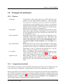
2.3
The input file
The SIMONA application independent preprocessor imposes the following syntax on the input file.
The input file is a structured ASCII file. From the input file only the first 258 columns are read. The
structure of the input file is designed by the application developer. He has divided the input into
separate blocks, which themselves may be subdivided into sub-blocks etc. in a hierarchical order.
The distinction between the (sub-)blocks is done through the use of keywords. The names of the
keywords as well as their hierarchical relation are chosen by the application developer.
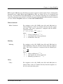
Block
A block is defined as all information (including sub-blocks)
between two keywords of the same level. The sequence of
(sub-)blocks related to keywords of the same level can be chosen
arbitrarily. Each (sub-)block can be specified only once, and
all data concerning that (sub-)block must be given at that place.
It is not allowed to add data for the same (sub-)block further
down in the input file. A keyword defines a block. Therefore a
defined block has to contain information, i.e. may not be empty.
This principle means that at least one sub-keyword of a defined
block ought to be defined in the input file, even when all these
sub-keywords are optional.
Five types of items can be distinguished:
Version 10.59, October 2013
5
User’s Guide WAQUA: General Information
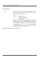
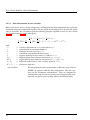
Keywords
reserved keyword
include
insert
1)
Keywords:
A keyword is defined by a sequence of letters and underscores only.
Keywords are case insensitive. The number of significant characters is imposed by the application developer, thus enabling the user
to abbreviate lengthy keywords or extend unclear keywords.
There are some reserved keywords which are used to forward special information. The following reserved keywords are available:
- INCLUDE:
Utilizing the keyword INCLUDE the user specifies that a data file
has to be included in the input file. For the included file the same
rules apply as for the original input file, except for the fact that it
may not contain any includes itself.
Usage (with text in [square brackets] being optional):
include [file =] filename
The include file name can contain an explicit path name. The use
of any indication of a parent directory (’..’) is allowed.
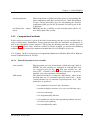
- INSERT:
Utilizing the keyword INSERT the user specifies that a file has to
be inserted in the input file. In the inserted file however, only data
are allowed, eventually with a number of heading comment lines.
The user specifies the contents of the inserted file by:
nheadings = –: number of heading lines, default = 0
number
= –: number of values to be read (mandatory)
format
= –: format to be used to read the values.
The following values are available for format:
• 0: free format (default)
• 1: unformatted
• 2: (10i6)
• 3: (10x, 12F5)
• 4: (16F5.0)
• 5: (12F6.0)
• 6: (10F8.0)
Note: the use of FORTRAN format implicates that tabulators are
not allowed as separators in the insert file.
Usage:
insert [file =] filename, [nheadings = ..], number = ..,
[format = ..]
The insert file name can contain an explicit path name. The use of
any indication of a parent directory (’..’) is allowed.
6
Chapter 2. About SIMONA
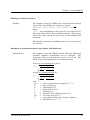
SET keyword
Numerical data
2)
Character strings
3)
Comment lines
4)
Version 10.59, October 2013
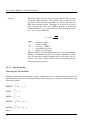
- SET:
With the keyword SET the user may set one of the following control flags or variables:
set echo:
echo input from present position
set noecho:
suppress echoing from present position
set nowritesds: suppress writing results of pre-processing to
the SDS file (supported by SIMONA applications unless stated otherwise)
set maxwarn:
<number>, defines the maximum number of
warnings that will be printed, default: the setting in the SIMONA environment file
set maxerror:
<number>, defines the maximum number of
errors that will be printed, default: the setting
in the SIMONA environment file
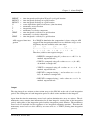
Numerical data:
A number is defined in the FORTRAN way, i.e. a row of symbols
from the group . 0 1 2 3 4 5 6 7 8 9 + -, i.e. dot, digits and signs,
ordered in the usual way: + - are only allowed at the first position and only one of both, furthermore, only one decimal point is
allowed in the total row while all digits may be repeated unrestrictedly; the row may be extended with d, e, D or E as in the standard
FORTRAN format.
Character strings:
A character string is everything that is placed between a begin- and
end-quote: ’ and ’. A quote is not allowed in the string itself.
Comment lines:
The user may add comment lines in the input file. These comment
lines are ignored by the program. Such comments may be of great
importance because they can clarify the meaning of the keywords
used. All text after a hash character (#) in an input line is considered to be comment (as is all text beyond the 258th column).
7
User’s Guide WAQUA: General Information
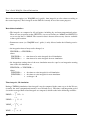
Separation characters
8
5)
Separation characters:
The following characters are recognized as separation marks, i.e.
they do not have a meaning themselves but do separate other items:
space
back-slash
\
slash
/
equal sign
=
open parenthesis (
close parenthesis )
comma
,
colon
:
semi-colon
;
tabulator
end of input line (i.e. position 259)
The user is advised to make full usage of the possibilities to structure his input (by using separation characters, comment lines, and
indentation). This will result in an input file that is clear and readable.
Chapter 3. About WAQUA
Chapter 3
About WAQUA
The text of this section about WAQUA originates for a large part from Rand Corporation Working
Draft WD-822-Neth, written by C.N. Johnson, A.B. Nelson and M.C. Fujisaki and later edited by
J. Vincent and G.J. Bosselaar for earlier versions of the WAQUA user’s guide.
Version 10.59, October 2013
9
User’s Guide WAQUA: General Information
3.1
Introduction to the system
This system is called WAQUA. It is used for two-dimensional hydro-dynamic and water quality simulation of well-mixed estuaries, coastal seas and rivers. As documented here, the system consists
of a pre-processing program, a program for actual simulation and a number of post-processing programs for graphics output and prints. The major part of the system is written in FORTRAN77, with
a minimum of computer dependent C code. It has been used on several mainframe and midrange
computers and workstations. It is large, complex, and expensive in computer resources.
3.1.1
Function of the system
simulation
graphics
data management
flexibility
10
The system can simulate hydrodynamics in geographical areas
which are not rectangular, and bounded by any combination of
closed boundaries (land) and open boundaries. Open boundaries
can drive the model by water levels, velocities, Riemann invariants,
discharges or distributed discharges, given either as time-varying
data or Fourier/harmonic functions of phase and amplitude at given
fre-quencies, or as a table, relating discharge with water level values. The system accounts for sources of discharge, such as rivers
or outfalls, for tidal flats, for islands and dams, movable barriers or
sluices and weirs. The water-quality computation handles several
constituents.
Such a simulation can generate great numbers of numbers. The
second function of the system is to display computations in a
highly visible way. Graphics include maps and time histories.
Maps show computations for a point in time over the entire water body. Time history graphs show computations across time at
one point in space. Time histories can also show computed and
observed data together, for verification of a model, or to show the
effect of proposed or hypothetical changes in the environment.
Some other functions of WAQUA can be grouped under the heading of data management. Input data are checked by a program and
printed in a (future) input report for easy inspection by the user
before the actual simulation, to minimize costly errors. The input
report will, together with the input file, be an effective documentation of the model.
Also, the system is flexible so that small models can be run on
small computers although large models require large computers
(especially for the simulation itself). The program sizes vary with
the size of the model, and the model can disregard various features of the system, including water-quality computation. Lastly,
the system simplifies the use of the computer so that the user can
concentrate on the research problem.
Chapter 3. About WAQUA
3.1.2
Features
simulation steps
graphics
reports
messages
modularity
Version 10.59, October 2013
When the system is fully used, the following steps are involved.
The user sets up the data for a model by the use of the documentation and input file of another model. Then the user has
that data checked, documented by print output, and filed by program WAQPRE. Then the simulation itself, program WAQPRO,
is run, generating print of computations and file output for postprocessing.
Displays or high-quality plots are an indispensable part of the system to show a large volume of information visually. Since the
simulation deals with two dimensions of space plus the time dimension, there are two kinds of displays, maps and time histories.
Maps are generally snapshots, or pictures throughout space at a
point in time. Time histories are time exposures, generally for a
point in space or a cross-section.
These types of postprocessing are possible with the WAQUA postprocessing programs at the moment available.
Two features of reports are mentioned here: self-documenting reports and separated run messages.
The self-documenting reports are those that print input data
and control parameters, especially the (future) preprocessor
(WAQPRE) input report. These minimize the user’s dependence
on separate, written documentation.
Run, error, and warning messages from programs can be printed
separately from reports, so that the success of a run can be determined without searching through a large volume of print. This is
especially useful where runs are made from remote terminals and
printing or viewing facilities are slow or otherwise inconvenient.
The water-quality feature of the system can be bypassed by giving no constituents. Likewise a model can omit time-varying
open boundaries, Fourier-driven openings, outfalls or constituent
sources, in fact any feature except the basic hydrodynamics.
11
User’s Guide WAQUA: General Information
model types
The user of the WAQUA system may use four types of grid systems:
• rectilinear coordinates;
• curvilinear coordinates;
• spherical coordinates;
• generalized spherical coordinates.
space varying wind and
pressure
user routines
12
The choice between the above mentioned ways of modelling an
area should be made in a very early stage of the modelling project
because it is vital for all model input preparing activities.
The choice is governed by the characteristics of the area to be modelled.
A curvilinear grid however may be more favourable in cases where
the area of interest is much smaller than the complete model area,
or when the physical characteristics of the area demand small grid
sizes on certain locations but allow at the same time larger grid
sizes in other spots. This may be the case in river applications
when an extensive winterbed is present.
Rectilinear/curvilinear models covering a relatively large part of
the globe lose accuracy due to the sphere shape of the earth. For
such models spherical coordinates is a good option.
In general WAQUA models cover a small area and spatial distribution of wind speed, wind direction and air pressure can be neglected. Spherical coordinate models however cover a considerable area where air pressure as well as wind speed and direction
vary. In those cases WAQUA allows the user to use the space varying wind and pressure feature.
WAQUA offers the user possibilities to simulate dissolved substances. Constituents such as salinity, pollutants or algae can be
modelled. As long as users deal with conservative dissolved substances, standard input facilities of the WAQUA system are sufficient.
Relations/reactions between these substances however should be
modelled by means of a user defined ’user routine’. The system
provides the heading of this routine. The user is responsible for
programming his own reaction kinetics.
Chapter 3. About WAQUA
3.1.3
Modelling with WAQUA
the art of modelling
model dimensions
open boundaries
well mixed basins
Version 10.59, October 2013
First of all, the system is not fool-proof; its answers are not necessarily realistic because its inputs require considerable judgement.
Modelling is an art to be learned, beyond the knowledge of physical characteristics of water bodies. The limitations of digital computers and numeric simulation need to be understood. Potentially,
after many computations, truncation errors can accumulate to a serious inaccuracy, due to a limited number of significant digits computers retain.
Fortunately, a model has been run for about 60 days with this system and there was no serious cumulative error. Many of the inputs,
such as diffusion coefficients, must be determined by judgement
and experimentation. A model should be verified, that is, matched
with observed data. Also, sensitivity tests should be made to obtain an impression of the effect that changing parameters has on
computational results.
Secondly, the water body should be of a practical size, to be simulated for a practical length of time. A model can get too large
for available computers or prohibitive in cost. The basic size of a
model is the number of grid spaces, and grid spaces should be small
enough for some accuracy. Waves should not be short compared to
grid space size, especially where eddies may be generated.
Long open boundaries should be placed at the edge of the grid.
For a rectangular grid this implies m = 1 or m = MMAX or n = 1
or n = NMAX, but for a curvilinear grid m = 1 and n = 1 are not
allowed (see also paragraph 3.2.1.3, computational grid tuning and
open boundaries). The advective terms normal to the boundary are
set to zero for a more stable boundary computation.
An estuary, coastal sea or river can be modelled appropriately if
it is well mixed that is, if one can assume no vertical velocity and
no horizontal velocity gradient from surface to depth. In that case,
no depth layering is required, and computation can be made on a
horizontal grid. The grid distance is in the range of 20 to 10,000
meters, and the depth is on the order of 10 meters. The grid dimensions are on the order of 100 by 100.
The basic computation is of water movement between grid points
and water level at each grid point. Optionally, the simulation will
compute transport of constituents, such as salinity, carried with water movement and concentration of constituents at each grid point.
Also with constituents computation no vertical gradients can be
simulated.
13
User’s Guide WAQUA: General Information
computational grid
monitoring
limitations
running programs
computational methods
14
Within this grid, an area can be designated in which the computations are made. This area is called the computational grid. Computations at all points on the computational grid are performed every
time step (where a time step is typically 1 to 2 minutes) for a simulated time of several days, usually.
Computations throughout the field (the computational grid) may be
printed and/or saved for later mapping (on the SDS file) at by the
user specified intervals (typically every 1 to 12 hours of simulated
time). To deal with the volume of computation and show connected
histories of change (in water level, for example), a relatively few
grid points (10 to 50) are chosen as stations. Computed values at
stations are printed and saved more frequently (typically every 5 to
10 minutes) on the SDS file for later display as time histories.
The water body should be well-mixed (with vertically integrated
velocity and concentrations) for two-dimensional simulation. This
is only one example of the physical and numerical limitations, to
indicate that a thorough knowledge of the system is required for
its successful use. Some detailed limitations are listed in program
user’s guides, especially the WAQPRE and WAQPRO guides.
There are no upper limits on the numbers of grid points, open
boundaries, sources, dams, barriers, islands, stations, or crosssections, or in the complexity of the shape of the computational
grid. However, the number of grids points in both the x- and ydirection should be at least three (thus NMAX ≥ 3 and MMAX ≥
3).
The information dealing with running the programs is available in
the Quick Reference Guide to WAQUA.
Some familiarity with the computational procedures and techniques used in WAQPRE and WAQPRO will help in designing a
model. While this subject will not interest all users, some knowledge of the sequence of operations may be valuable if difficulties
arise during a simulation. In most sections of chapter 3.4: General
hydrodynamics, that describe the different properties of the system, subsections with information on computational methods are
included.
Chapter 3. About WAQUA
3.2
Geometry
3.2.1
Computational grid
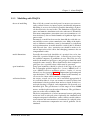
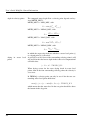
3.2.1.1
Computational grid structure
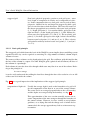
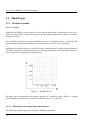
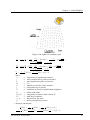
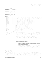
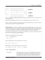
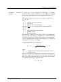
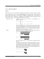
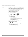
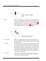
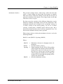
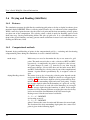
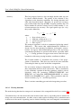
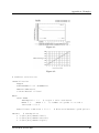
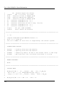
WAQUA grid
The WAQUA grid is illustrated in fig. 3.1. In modelling an estuary coastal sea or river, a rectangular geographical area is chosen,
where its edges need not correspond with north, east, south and
west. A grid is laid on the rectangular area, where the square grid
space size in meters is chosen, and the number of grid spaces in the
two dimensions, NMAX and MMAX, are chosen. The grid direction from left to right corresponds to the m-direction for grid space
subscripts and to the u-velocity. The upward direction corresponds
to the n-direction for subscripts and to the v-velocity.
Figure 3.1: Default computational grid with arbitrary openings
type of grid
Version 10.59, October 2013
Note: There are effectively one fewer row and column of velocities
then water levels on the right and the top.
Either a rectangular grid, a spherical grid or a curvilinear grid may
be chosen. In case of a curvilinear grid a file with curvilinear coordinates has to be provided (see section 2.5.1.2 in the user’s guide
WAQPRE).
15
User’s Guide WAQUA: General Information
staggered grid
3.2.1.2
Four basic physical properties pertain to each grid space: water
level, depth, u-component of velocity and v-component of velocity. In the computation there are four grids, one for each of these
properties, identical in size and shape but staggered by half a grid
space in one direction or both directions. The lower left corner of
the chosen geographical area coincides with water level grid point
(1, 1). Depth grid point (1, 1) is translated half a grid space to the
right and above, so that depth grid point (1, 1) falls midway between water level grid points (1, 1) and (2, 2). The u-velocity grid
point (1, 1) lies half a grid space to the right, so that it lies midway
between water level points (1, 1) and (m = 2, n = 1). The v-velocity
grid point lies midway between water level points (1, 1) and (m =
1, n = 2).
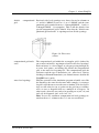
Basic grid principle
The staggered grid, which forms the basis of the WAQUA system, implies that a modelling system
organised in this way can be regarded as consisting of a large number of linked, column shaped,
volumes of water.
The corners of these volumes are the depth points in the grid. For rectilinear grids this implies that
the base of the column is a square. For other WAQUA grids (spherical and curvilinear) the base of
the columns is a quadrangle.
Each volume of water has four sides through which water may flow in or out of the volume. Referring to the principle of:
in = out + storage
it can be easily understood that adding the four flows through the four sides results in a rise or fall
of the water level inside the volume.
Fig. 3.5 gives a good impression of the implications of the staggered grid principle.
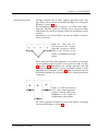
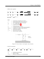
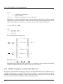
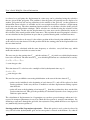
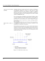
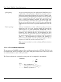
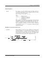
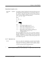
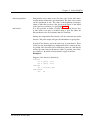
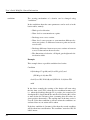
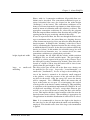
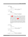
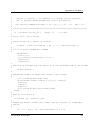
computation of depth values
Usually the average depth is used on the boundaries of a grid cell
for the computation of the flow in or out of the control volume.
The water levels are averaged perpendicular to the cell boundary
and the depths are averaged along the boundary; see fig. 3.2.
This approximation of the cross section normally ensures an accurate computation of the mass transport through the boundary of
the control volume. However, in close vicinity to steep bottom
gradients, as at drying flats and the change-over of winter-bed to
summer-bed, the average approach may lead to an inaccurate representation.
16
Chapter 3. About WAQUA
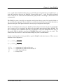
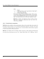
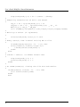
tiled depth approach
For those situations the so-called ’upwind’-approach is more suitable. This is discussed more in detail in the chapter on ’Drying and
Flooding’ (section 3.6).
For determining the depths we propose a so-called ’tiled depth’approach. Then the depth at a velocity point is equal to the minimum depth at the water level points of the two surrounding control
volumes.
Alternatively, it is also possible to specify the depths on input at
water level points.
Figure 3.2: Wet cross section based for the "average
approach" (depth in velocity
point is the average of the
depths in neighbouring depth
points)
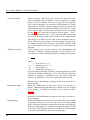
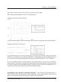
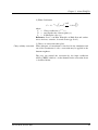
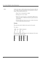
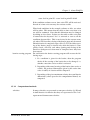
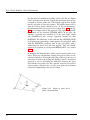
When using the tiled depth approach, it is possible to represent
a small channel (narrow gully) of one grid cell width, see Fig.
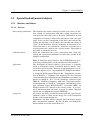
3.2 and Fig. 3.3. Furthermore, the ’average approach’ will lead
in shallow areas to so-called ’screens’ (in Dutch ’schotjes’) in the
tangential (or y-)direction, see Fig. 3.4. This is caused by the fact
that bottom gradients in y-direction affect the drying behaviour in
x-direction.
Figure 3.3: Wet section based
on a "tiled depth approach"
(depth in velocity point is the
minimum of the depths in
neighbouring depth points)
For a more detailed description we refer to the chapter concerning
’Drying and Flooding’ (section 3.6).
Version 10.59, October 2013
17
User’s Guide WAQUA: General Information
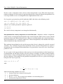
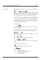
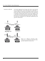
Figure 3.4: Screens in tangential direction occur when
the depth in a velocity point
is computed as the average
depth value of the neighbouring depth points
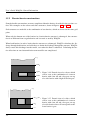
3.2.1.3
Computational grid tuning and open boundaries
non rectangular comp.
grid
The simulation program requires that open boundaries (e.g. tide
openings) where measured tide or river data are given to drive the
model, are on the edge of the computational grid. Where existing
tide gauges are located so as not to fit a rectangle, a non-rectangular
computational grid is fitted to the tide openings. Also, a computational grid may be defined, for the purpose of limiting computations, to an area of the grid that closely corresponds to the actual
shape of the water body, for efficiency.
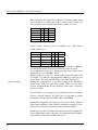
Figure 3.5: Control volume
of the continuity equation of
the finite difference representation in WAQUA
18
Chapter 3. About WAQUA
default
grid
computational
Previously tide level openings were always located at columns m
= 1 and m = MMAX or rows n = 1 or n = NMAX, and the computational grid extended from m = 2 through MMAX - 1 and n =
2 through NMAX - 1 (rectangular). This is still the default, if no
special computational grid is defined. Note that the ’default computational grid enclosure’ is superimposed on all tide openings.
Figure 3.6: Flow cross
section
computational grid enclosures
water level openings
Version 10.59, October 2013
The computational grid within the rectangular grid is defined by
one or more enclosures, superimposed on all water level openings.
Each enclosure is a closed figure or polygon passing through (m,
n) water level points, and falling just outside the computational
grid, as the water level openings do. The computational grid, the
enclosures and the type of boundaries (viz. water level, velocity,
discharge or Riemann boundaries) are defined in more detail in the
WAQPRE user’s guide.
With the extension of the simulation program to handle cases like
the North Sea, the same idea becomes more complex. A rectangular grid is still chosen to cover the area to simulate. Tide level openings are still related to (m, n) points on the grid, but as columns,
rows, or now as diagonals that are a multiple of 45 degrees. In
other words, where the two ends of an opening are at (m1, n1) and
(m2, n2) for diagonals, |m2 - m1| = |n2 - n1|.
Note: In case of a curvilinear computation tide level openings situated on the m = 1 column or the n = 1 row are not allowed.
19
User’s Guide WAQUA: General Information
velocity openings
discharge openings
Where velocities rather than water levels have been measured,
velocity openings may be defined. Velocity openings are single
points or rows or columns on the (m, n) grid, but not diagonals,
since velocity openings are associated with horizontal or vertical
components of velocity. Velocity openings also lie just outside the
computational grid, but within the defined grid enclosure. In the
space-staggered grid, velocity points lie between water level points
(see fig. 3.1). For a given (m, n) index its velocity points ’-’ and ’|’
lie to the right and above the ’+’ water level point. This means that
for velocity openings on the left or bottom of the computational
grid, their (m, n) indices are the same as those included in the enclosure. However, on the right, a velocity opening is assigned one
m-column to the left of the enclosure, and velocity openings at the
top of the computational grid are assigned one n-row below the
enclosure.
If the discharge rates at some points of the computational grid
enclosure are known, discharge openings may be defined. Local velocities are derived from discharges according to the formula:
v=
Q
H·∆x
where:
v
= flow velocity (m/s)
Q
= discharge rate (m3 /s)
H
= water depth (m)
∆x = width of the opening (m)
A special form of discharge opening is an opening with a so-called
’automatic’ distributed discharge: a user specified total discharge
through an opening is distributed over the points along the
opening, accounting for local water depth and bottom friction.
Riemann openings
Q-H openings
20
Restrictions for the discharge openings are the same as for the velocity openings.
When the combination of both water levels and velocities is
known, a Riemann invariant boundary condition can be assigned
to an opening. A further description can be found in section
3.4.2.3.
Restrictions for the Riemann openings are the same as for the velocity openings.
When the relation between water level and total discharge through
an opening is known (e.g. in rivers), the water level at the opening
can be computed during the computation from the total discharge.
Q-H type of openings are specified with boundary points located
as for water level openings, with the restriction to only horizontal
or vertical open boundaries (like velocity openings).
Chapter 3. About WAQUA
3.2.2
Physical geometry
dry points or dams
screens
weirs
barriers or sluices
Version 10.59, October 2013
The modeller may define certain grid points to be permanently dry
points, overriding the description of depth throughout the field.
This provides a means to make a dam or causeway through the
water body with considerable depth at either side.
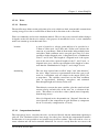
The modeller may define screens at certain velocity points. This
enables the modeller to create dams without width, to simulate for
instance groynes, which have a width small compared with the grid
size.
The modeller may define certain grid points to be weirs, which
are fixed, non-movable constructions causing energy losses due to
constriction of flow.
The modeller may define certain grid points to be sluices or barriers, which are a time-varying constriction on velocity in the udirection or the v-direction.
21
User’s Guide WAQUA: General Information
3.3
Model types
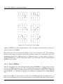
3.3.1
Rectilinear models
3.3.1.1
General
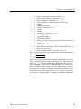
Originally the WAQUA system could only cope with rectilinear grids. In large parts of the user’s
guide a rectilinear grid is assumed, but in most cases the documentation is also valid for curvilinear
and spherical grids.
For a rectilinear grid there is a simple relation between (m, n) coordinates and (x, y) locations. The
input and output of the subsystems however refer in most cases to the (m, n) coordinates.
Defining the rectilinear grid can be carried out easily. Numerically the rectilinear model equations
are simpler and because of that the model is faster during computation. The mathematical accuracy
can be assessed easier than for the other grid types.
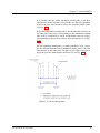
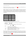
Figure 3.7: Rectilineair grid
The figure gives an impression of the regular structure of a rectilinear model. There is a straight
forward relation between the (m, n) model coordinates and an (x, y) reference.
3.3.1.2 Mathematical description differential equations
The following equations govern the rectilinear WAQUA computation:
22
Chapter 3. About WAQUA
• shallow water equations
∂u
∂t
√
√
2
2
∂ζ
+v
+ u ∂u
+ v ∂u
− f v + g ∂x
+ gu Cu2 (h+ζ)
=
∂x
∂y
∂v
∂t
+
∂v
u ∂x
∂ζ
∂t
+
∂
∂x
+
∂v
v ∂y
(Hu) +
+f u+
∂
∂y
∂ζ
g ∂y
+ ν
+ ν
√
√
+ gv
ρa Cd Wx Wx2 + Wy2
ρw (h+ζ)
u 2 +v 2
C 2 (h+ζ)
=
ρa C d W y
Wx2 + Wy2
ρw (h+ζ)
∂2u
∂ x2
∂2 v
∂ x2
+
∂2u
∂y2
+
∂2 v
∂y2
(Hv) = 0
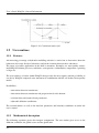
where:
u,v
ζ
h
H
f
g
C
W x , Wy
Cd
ρa , ρw
υ
components of depth mean current u
˜
water elevation above plane of reference
water depth below plane of reference
h + ζ (refer to Fig. 3.8)
parameter of Coriolis
acceleration due to gravity
coefficient of Chezy to model bottom roughness
˜
components of surface wind velocity W
wind drag coefficient
density of air and water
eddy-viscosity coefficient
=
=
=
=
=
=
=
=
=
=
=
Figure 3.8: Layer of water = water depth + water elevation
• dissolved constituents:
∂
∂t
(Hc) +
∂
∂x
(Huc) +
∂
∂y
(Hvc) =
∂
∂x
∂c
HDx ∂x
+
∂
∂y
∂c
HDy ∂y
+ Sc
where:
C
Sc
Dx , Dy
=
=
=
constituent concentration
sources or sinks
diffusion coefficients in x- and y-direction
Version 10.59, October 2013
23
User’s Guide WAQUA: General Information
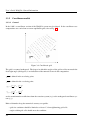
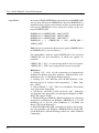
3.3.2
Curvilinear models
3.3.2.1
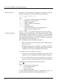
General
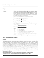
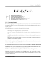
In the 1980’s a curvilinear version of the WAQUA system was developed. In the curvilinear case
computations are carried out on a non-equidistant grid, refer to Fig. 3.9.
Figure 3.9: Curvilineair grid
The grid is assumed orthogonal. The degree in which the angles of the grid used do not match the
ideal right angle (90 degrees) is an indication of the numerical error in the computation.
√
√
gηη is defined in the u-velocity point.
gξξ is defined in the v-velocity point.
gξξ =
∂x
∂ξ
gηη =
∂x
∂η
2
2
+
+
2
∂y
∂ξ
2
∂y
∂η
are the transformation coefficients from the cartesian system (x,y) to the orthogonal curvilinear system (ξ,η).
Rules of thumb to keep the numerical accuracy acceptable:
• grid size variations should be limited to a factor 1.3 for neighbouring grid cells;
• angles within grid cells should meet the condition:
24
Chapter 3. About WAQUA
100 * cos (angle) < 2 (deviation of approximately 1.2 degrees).
Cells not meeting this criterion should be examined by a model engineer.
Curvilinear grids may be applied in cases where the area of interest is much smaller then the complete model. Another case in which curvilinear models prove to be a good alternative occurs when
the physical characteristics of the area involved show a great variety. An example of this phenomena is a Dutch river with a relatively narrow summer bed and a wide winter-bed. To model the flow
(discharge) through the summer bed properly, a small grid size is required. The winter-bed however
is shallow and small grid sizes are not necessary when modelling the discharge and the flow pattern
in that area.
The curvilinear grid must be given to the WAQUA system as an input file, the so called RGF file.
The format of this file is straight forward ASCII. The RGF file can be used as direct input for the
WAQPRE subsystem.
The RGF file is the output of a grid generating process for which a grid generator program should
be used. The WAQUA system is not equipped with a grid generator.
3.3.2.2
Mathematical description differential equations
The following equations govern the curvilinear WAQUA computation:
• shallow water equations:
∂u
∂t
∂v
∂t
∂ζ
∂t
+
+
+
√
√
2 ∂ g
∂ g
u ∂u
√
+ √gvηη ∂u
+ √uvg∗ ∂ηξξ − √vg∗ ∂ξηη
gξξ ∂ξ
∂η
√
√
ρa Cd Wξ Wξ2 +Wη2
u2 +v 2
+gu C 2 (h+ζ) =
+ √gvξξ ∂A
ρw (h+ζ)
∂ξ
− fv +
−
√
√
g ∂ζ
gξξ ∂ξ
v ∂B
gηη ∂η
√
√
2 ∂ gξξ
∂ξ
u ∂v
v ∂v
uv ∂ gηη
√
√u
√
√
+
+
−
+ f u + √ggηη ∂η
gξξ ∂ξ
gηη ∂η
g∗ ∂ξ
g∗ ∂η
√
√
ρa Cd Wη Wξ2 +Wη2
2 +v 2
gv C 2u(h+ζ)
=
+ √gvηη ∂A
+ √gvξξ ∂B
ρw (h+ζ)
∂η
∂ξ
√1 ∂
g∗ ∂ξ
√ Hy gηη +
√1 ∂
g∗ ∂η
√ Hy gξξ = 0
where:
A=
√1
g∗
h
∂
∂ξ
B=
√1
g∗
h
∂
∂ξ
i
√ ∂ √ u gηη + ∂η
v gξξ
i
√ √ ∂
u gηη − ∂η v gξξ
and:
Version 10.59, October 2013
25
User’s Guide WAQUA: General Information
u,v
ζ
h
H
f
g
C
Wξ , Wη
Cd
ρa , ρw
υ
gξξ , gηη
g∗
=
=
=
=
=
=
=
=
=
=
=
=
=
components of depth mean current u
˜
water elevation above plane of reference
water depth below plane of reference
h+ζ
parameter of Coriolis
acceleration due to gravity
coefficient of Chezy to model bottom roughness
˜
components of surface wind velocity W
wind drag coefficient
density of air and water
eddy-viscosity coefficient
transformation coefficients (see par. 3.3.1.1)
gξξ · gηη
• dissolved constituents:
∂
∂t
(Hc) +
√1 ∂
g∗ ∂ξ
where:
c
Sc
Dξ , Dη
√1 ∂
g∗ ∂ξ
HDξ
=
=
=
√ Huc gηη +
√
gηη
√g ∂c
ξξ ∂ξ
+
√1 ∂
g∗ ∂η
√1 ∂
g∗ ∂η
HDη
√ Hvc gηη =
√g
√ ξξ ∂c
gηη ∂η
+ Sc
constituent concentration
sources or sinks
diffusion coefficients in ξ- and η-direction
3.3.3
Spherical coordinates models
3.3.3.1
General
When the area to be modelled covers a considerable part of the globe, the assumption of a flat
(rectilinear or curvilinear) model is no longer valid. For such a model area a spherical coordinates
WAQUA model can be defined, refer to Fig. 3.10.
The grid size is no longer defined in meters but in degrees. Users are advised to choose for spherical
grids with an n-axes pointing North and an m-axes pointing East. Spherical grids with m- and n-axes
not coinciding with longitude and latitude are possible but not convenient in use.
3.3.3.2
Mathematical description differential equations
The following equations govern the spherical coordinates WAQUA computation:
• shallow water equations:
26
Chapter 3. About WAQUA
Figure 3.10: Spherical coordinates grid
∂u
∂t
+
u
∂u
R cos φ ∂λ
+
v ∂u
− uvtgφ
− 2Ωv
R ∂φ
R
√
ρa Cd Wλ Wλ2 +Wφ2
ρw (h+ζ)
∂v
∂t
+
u
∂v
R cos φ ∂λ
+
ρw (h+ζ)
∂ζ
∂t
+
1
∂
(Hu)
R cos φ ∂λ
where:
u,v
ζ
h
H
Ω
g
C
R
Wξ , Wη
Cd
ρa , ρw
pa
=
=
=
=
=
=
=
=
=
=
=
=
−
2
v ∂v
+ u Rtgφ + 2Ωv
R ∂φ
√
ρa Cd Wφ Wλ2 +Wφ2
+
1
∂
(Hv
R cos φ ∂φ
g
∂ζ
R cos φ ∂λ
sin φ −
2
2
∂pa
1
ρw R cos φ ∂λ
sin φ +
−
√
+v
+ gu C 2u(h+ζ)
=
g ∂ζ
R ∂φ
√
2
2
+v
+ gv C 2u(h+ζ)
=
1 ∂pa
ρw R ∂φ
cos φ) = 0
components of depth mean current u
˜
water elevation above plane of reference
water depth below plane of reference
h+ζ
angular speed of the earth’s rotation
acceleration due to gravity
coefficient of Chezy to model bottom roughness
radius of the earth
˜
components of surface wind velocity W
wind drag coefficient
density of air and water
surface atmospheric pressure
• dissolved constituents:
∂
1
∂
1
∂
(Hc) + R cos
(Huc) + R cos
(Hvc cos φ) =
∂t φ ∂λ φ ∂φ
1
∂
1
∂c
1
∂
1 ∂c
HD
+
HD
cos
φ
+
λ R cos φ ∂λ
φ R ∂φ
R cos φ ∂λ
R cos φ ∂φ
Version 10.59, October 2013
Sc
27
User’s Guide WAQUA: General Information
where:
c
Sc
Dλ , Dφ
=
=
=
constituent concentration
sources or sinks
diffusion coefficients in λ- and φ-direction
Note: There is a strong relationship between the equations for curvilinear coordinates and the
equations for spherical coordinates. Define a fixed Cartesian frame through the origin of the
*
earth, then the spherical coordinates of a point r on the earth’s surface are given by:
*
r = (x, y, z)T = (λ, φ, R)T
with:
x = R · cos φ · cos λ,
y = R · cos φ · sin λ,
z = R · sin φ.
The transformation coefficients are:
√
∂~r gλλ = ∂λ
√
∂~r gφφ = ∂φ






=










=









−R cos φ sin λ 
 = R cos φ,



0

−R sin φ cos λ 



−R sin φ cos λ 
 = R



Rcosφ
−R cos φ sin λ
Replacing ξ and η by:
√ √
√
√
ξ = λ, η = φ ⇒ gξξ = gλλ gηη = gφφ
Substituting these formulas in the equations for a curvilinear grid, the equations in spherical
coordinates without Coriolis-force and viscosity terms are derived.
3.3.4
Models using space varying wind and pressure
For all three earlier mentioned model types the Space Varying Wind and Pressure (SVWP) feature is
available. It enables the user to drive his model with an extensive set of time dependent and spatial
distributed wind boundary conditions. Fields of wind directions, wind speeds or stresses and air
pressures can be processed by WAQUA, while interpolating in time.
28
Chapter 3. About WAQUA
A (λ, φ) grid can be transformed into an (x, y) grid. If the pressure parameters are required in (λ, φ)
form, they should be offered to the WAQUA system in their own (λ, φ) grid. The wind grid should
have at least the size of the water movement and quality model. An overlap is allowed and even
recommended.
The WAQUA system is not able to extrapolate wind related data to parts of the model which are
not covered by the wind grid. Flat (rectilinear or curvilinear) models may be provided with a flat or
spherical wind grid. The spherical models can only cope with spherical wind grids.
The file describing the time and space distributed wind and pressure data may be of considerable
size. In most cases it is produced and delivered by the dutch meteorological office (KNMI). The
file is transformed into a SIMONA SDS file by the WAQUA subsystem WAQWND. The name of
this special SDS file should be stated in the WAQPRE input under ’general space_var_wind’. The
format of the files involved is described in the WAQUA system’s documentation.
Instead of wind speeds it is also possible to provide WAQUA with wind stresses. These stresses
must have been computed as:
Sx = ρa Cd Wx
q
Sy = ρa Cd Wy
q
Wx2 + Wy2
Sx , Sy
Wx , Wy
Cd
ρa
Wx2 + Wy2
= components of surface wind stress
˜
= components of surface wind velocity W
= wind drag coefficient
= density of air
Version 10.59, October 2013
29
User’s Guide WAQUA: General Information
3.4
3.4.1
General hydrodynamics
Features
time step
interpolation
time interpolation
space interpolation
tide openings
30
The full time step in minutes is chosen and given to WAQPRO
through WAQPRE. At the first half time step, u-velocities and
resultant water levels are calculated and also separate v-velocities
(explicit). At the second half time step, v-velocities and resultant
water levels are calculated together with separate u-velocities
(explicit). This means that u- and v-components of velocity are
never completely synchronized in time (staggered time step).
Also, the computation has alternating direction, that is, u-velocities
are calculated with the m subscript varying faster, and the n subscript varies faster for v-velocity.
All time-varying inputs are interpolated across time, and inputs at
open boundaries are also interpolated across space.
Interpolation across time occurs for the time series at tide openings
and at discharge points, which can be equidistant or not. The value
at the beginning of interpolation is either the previous value given
in the input, or the initial value (given or assumed) (see paragraph
3.4.2.3).
Interpolation across space occurs at open boundaries, where inputs
are given at the two ends of the opening, and values at intervening
grid points on the opening are calculated by interpolation. Space
interpolation is done to tide level or velocity at Fourier or timevarying openings, and to constituent concentration and - only initially - constituent return time (see section 3.8).
The main hydrodynamic forcing function is observed tide at open
boundaries or tide openings. Historically the simulation has accepted water level values at a regular time interval. Extensions to
the simulation accept not only velocity, Riemann or discharge values at a regular time interval but also Fourier functions of timevarying values of either water level, velocity, Riemann or discharge.
For application of WAQUA to river hydraulics, boundary conditions can be specified as a total (upstream) discharge or as a relation between total (downstream) discharge and water level.
The Fourier functions have any number of angular frequency components with corresponding phase and amplitude values. The simulation interpolates phase and amplitude across the space of the
open boundary before transforming back to the time domain and
interpolating across time.
Chapter 3. About WAQUA
wind interpolation
non-hydrostatic computation
3.4.2
Time interpolation of global wind takes place by interpolating the
polar components wind angle and wind speed. Time interpolation
of space varying wind takes place by interpolating the cartesian
components wind speed in the X-direction and wind speed in the
Y-direction.
TRIWAQ has the possibility to take non-hydrostatic effects for
free-surface flows into account.
Computational methods
In this section an overview is given of the time advancement procedure of state variables and accuracy considerations. Furthermore, forcing functions that drive the simulation are mentioned, as
well as the computation of time integrals. The drying and flooding procedures will be described
in section 3.6.2. Chezy values, which are defined at velocity locations, are related to the Manning
coefficient. A full account of the numerical method that is used in WAQUA is given in:
G. S. Stelling, On the Construction of Computational Methods for Shallow Water Flow, Rijkswaterstaat Communications no 35/1984.
3.4.2.1
Time advancement of state variables
state variables
ADI scheme
The integration proceeds in increments of half time steps (half of
TSTEP). All state variables are computed in each half time step
on a staggered grid (see Fig. 3.1). The state variables are: the
water level ζ, velocities u and v in x and y directions, respectively
(initially zero), and constituent concentrations.
The numerical method is a composite ADI scheme, where in the
first half time step v is calculated separately from u and ζ. In the
second half time step u is calculated separately from v and ζ. The
method has as properties:
• it is symmetrical over the x and y directions,
• it attains its highest accuracy over every two half time steps,
• it is mass conserving,
• it is computationally efficient,
• it is suitable not only for time-dependent problems, but also
for steady state problems,
• it is unconditionally stable.
Version 10.59, October 2013
31
User’s Guide WAQUA: General Information
accuracy
This last property however, does not imply that the time step can
be chosen without bounds. The quality of the solution is also
dependent on the boundary conditions, the forcing functions and
other time-dependent input. Therefore, in practice the accuracy
puts a limit on the time step (TSTEP). In many problems the
Courant number Cf is a relevant measure. For equal spatial steps
(dx = dy) it can be defined by
√
Cf = ∆t ·
2gH
dx
where:
H = total water depth
Cf = Courant number
∆t = time step = TSTEP
g
= acceleration of gravity
dx = spatial step (grid space)
Thus, an estimate for the maximum value of ∆t can be determined.
However, a maximum limit on ∆t is problem dependent. In some
cases the geometry can put a limiting factor on the time step ∆t,
because of accuracy reasons. There is no time smoothing present
in the integration procedure.
3.4.2.2
Time integration
Time integrals, 2D simulation
During the simulation ’time integrals’ may be computed over one or more successive periods. For
each integration period five time-integrated flow-related integrals are computed, which results in the
following variables:
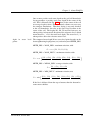
t+T
R
DEPINT =
(H + ζ) · dt
t
UPINT =
t+T
R
u · dt
t
VPINT =
t+T
R
v · dt
t
DISUNT =
t+T
R
(H + ζ)u · dt
t
DISVNT =
t+T
R
t
where:
32
(H + ζ)v · dt
Chapter 3. About WAQUA
DEPINT
DISUNT
DISVNT
H
ζ
T
u
UPINT
v
VPINT
=
=
=
=
=
=
=
=
=
=
time-integrated total depth at W(ater) L(evel) grid location
time-integrated discharge at u-grid location
time-integrated discharge at v-grid location
water depth below plane of reference, (time-invariant)
momentary water elevation
integration period
momentary u-velocity component
time-integrated u-velocity at u-grid location
momentary v-velocity component
time-integrated v-velocity at v-grid location
ADI staggered time integration
In a WAQUA-simulation the computation is done, using an ADI
staggered time integration method over two half time steps, so not
all primary data are available at the same time:
ζ,v
ζ,u
ζ,v
ζ,u
I---------I---------I---------I----- ....
t
t + 0.5 · dt t + dt t + 1.5 · dt
Therefore (with k a non-negative integer):
• DEPINT is computed using all ζ-values at t = t + 0.5 · k · dt;
method: trapezoidal rule;
• UPINT is computed using all u-values at t = t + (k + 0.5) ·
dt; method: rectangle rule;
• VPINT is computed using all v-values at t = t + k · dt;
method: trapezoidal rule;
• DISUNT is computed using ζ- and u-values at t = t + (k +
0.5) · dt; method: rectangle rule;
• DISVNT is computed using ζ- and v-values at t = t + k · dt.
method: trapezoidal rule.
Output
The time integrals are written as time-variant array to the SDS file at the end of each integration
period. The ending time of each integration period is added as time attribute for the integrals.
Apart from the time the momentary water levels and an administrative array are written. The administrative array contains time information for all time integrals: starting time of the integration
period, ending time of the integration period and the integration period duration. The momentary
water levels are included for later appliance of an ’integrated continuity equation’. Therefore the
momentary water levels are also added by an extra write at t = TFINT (starting time integration
process).
Version 10.59, October 2013
33
User’s Guide WAQUA: General Information
Due to the restart option (see WAQPRE user’s guide), time integrals are also written according to
the restart frequency. These integrals on the SDS file can only be used for restart purposes.
Restrictions/reminders
• The integrals are computed at all grid points, including dry and non-computational points.
There are two exceptions to that: DISUNT is set to zero for line m = MMAX and DISVNT is
set to zero for line n = NMAX. The reason for that is that not all necessary data are available
at those grid locations.
• Permanent restart (see WAQPRE user’s guide) is only allowed under the following restrictions:
• the integration interval may not be changed, so
TIINTEGRold = TIINTEGRnew
where:
TIINTEGRold
TIINTEGRnew
=
=
time interval to write integrals for old simulation
time interval to write integrals for new simulation
• the integration starting time of the new simulation must be equal to an integration starting
time of the old simulation, so:
TFINTEGRold = TFINTEGRnew
where:
TFINTEGRold
TFINTEGRnew
k
=
=
=
first time to write integrals for old simulation
first time to write integrals for new simulation
an integer > 0
Time integrals, 3D simulation
During a TRIWAQ simulation ’time integrals’ may be computed in the same way as in the 2D case
(actually, the same computational routine is used in both cases). This time each integration period
seven time-averaged flow-related integrals are computed, which results in the following variables:
ZKINTk =
t+T
R
ZKk · dt
t
UPINTk =
t+T
R
Uk · dt
t
VPINTk =
t+T
R
Vk · dt
t
WINTk =
t+T
R
t
34
ωk · dt
Chapter 3. About WAQUA
WPHINTk =
t+T
R
W physk · dt
t
DISUNTk =
t+T
R
Uk Hk · dt
t
DISVNTk =
t+T
R
Vk Hk · dt
t
where:
ZKINTk
UPINTk
VPINTk
WINTk
WPHINTk
DISUNTk
DISVNTk
ZK k
Uk
Vk
ωk
W physk
Hk
T
=
=
=
=
=
=
=
=
=
=
=
=
=
=
time-averaged position of layer interface with index k at W(ater)L(evel)-grid location
time-averaged u-velocity with index k at u-grid location
time-averaged v-velocity with index k at v-grid location
time-averaged Omega-velocity with index k at WL-grid location
time-averaged Wphys-velocity with index k at WL-grid location
time-averaged discharge at u-grid location with index k
time-averaged discharge at v-grid location with index k
momentary position of layer interface with index k
momentary U-velocity component of layer k
momentary V-velocity component of layer k
momentary Omega-velocity component of layer k
momentary component of physical vertical velocity of layer k
momentary thickness of layer k
integration period
ADI staggered time integration
Like in the WAQUA-simulation, the computation in a TRIWAQsimulation is done using an ADI staggered time integration
method:
ZKk ,Vk ,ωk ZKk ,Uk ,ωk ZKk ,Vk ,ωk ZKk ,Uk ,ωk
I-----------I-----------I-----------I---.....
t
t+0.5dT
t+dT
t+1.5dT
With i a (non-negative) integer:
• UPINTk , VPINTk , DISUNTk and DISVNTk are computed
in the WAQUA simulation.
• ZKINTk , WINTk and WPHINTk are computed using all values of ZKk at all t = t + 0.5 · i · dt using a trapezoidal rule.
Lagrangian displacements
The general idea In this section a description is given of the option in WAQUA/TRIWAQ concerning the calculation of Lagrangian displacements of points. In the standard hydrodynamic calculation, u- and v-velocities are calculated at fixed positions at a certain time. So, if a water mass
Version 10.59, October 2013
35
User’s Guide WAQUA: General Information
is released at a grid point, the displacement in a time step can be calculated using the velocities
that are given in that grid point. The problem is that the point will generally not be displaced to
another grid point but will end up somewhere in the middle of the grid cell. At that position no
information about velocities is available and it is not straight forward to calculate a displacement
for the next time step. The above mentioned option enables us to calculate velocities in the grid cell
itself with some interpolation technique. These velocities are calculated using the velocities of the
adjacent grid points. In this way the displacement of a water mass can be calculated by means of
the velocities at the actual position of the water mass. This explains the word Lagrangian: velocities
are not calculated at fixed positions in space but at a position moving with a certain water mass.
A quantity that also has to be stored, is the relative position of the released point within the grid cell
at the end of every time interval. For this position will be the starting point of the displacement over
the next time interval.
Displacements are calculated with the same frequency as velocities, every half time step, which
makes the method second order accurate in time.
The user can give the starting time Tstart and the end time Tend of period over which displacements
have to be calculated. The time interval Tint over which displacements are calculated has to satisfy:
k1 × Tint = Tend − Tstart
k1 some integer value
This time interval Tint also has to be a multiple of the hydrodynamic time step dt:
k2 ×dt = Tint
k2 some integer value
The user has two possibilities concerning initialization at the start of the time interval Tint :
• points can be initialized at the beginning of each interval Tint and will be replaced to their
starting positions. In this way the user is enabled to calculate displacements during separate
time intervals.
• point will start at the beginning of an interval Tint from the position they have reached the
previous time interval. This gives the possibility to calculated trajectories over a longer period
which are quite smooth.
The calculation of displacements in a Lagrangian way can have great advantages when one is interested in transport phenomena in areas in which the flow pattern is strongly non-uniform. By
following a water mass through the grid cells, the trajectories along which the masses are displaced
are (numerically) better reproduced.
Starting position of the Lagrangian trajectories When this option is used, a point is released in
every 3D-cell of the hydrodynamic grid, and an extra point is released at the bottom. So, when N
36
Chapter 3. About WAQUA
layers in the vertical are used, N+1 points are released per grid column.
The starting position within the cells is in the depth points:
Starting position in the horizontal grid:
A point with index (M,N) in the horizontal grid will start from a depth-grid point with index (M,N).
Starting position in the vertical grid:
A point with index k in the vertical grid will start at the upper layer interface of the grid cell with
index k+1 (or the bottom of the grid cell with index k). Consequently, the point with index kmax in
the vertical grid will start from the bottom of the grid cell with index kmax, i.e. the sea bottom.
In case the starting position of a point would be a land point and one or more of the surrounding
points would be a wet point, it is dis-placed a small distance in the direction of the wet point in order
to enable the point to move with the flow from its starting position. If all the surrounding points are
situated on land the before mentioned point will evidently not move.
Interpolation of the velocities in horizontal direction It has already been mentioned that, in
order to obtain values for the various velocity components at the actual positions of the released
points, it is necessary to interpolate using the velocities at the grid points.
Version 10.59, October 2013
37
User’s Guide WAQUA: General Information
For the u- and v-components of the velocity a linear interpolation is used. This rather simple interpolation technique was chosen after it appeared that the more advanced bilinear interpolation led to
a too large number of cases to distinguish in the neighbourhood of the coast.
So, if a point is present in the grid cell with index (M,N) this leads to the following result:
uint = f x · u(M, N ) + (1 − f x) · u(M − 1, N )
vint = f y · v(M, N ) + (1 − f y) · v(M, N − 1)
where fx, fy is relative position of a point in a grid cell:
0 < fx ≤ 1
0 < fy ≤ 1
The vertical velocity component is not interpolated horizontally.
Interpolation of the velocity components in vertical direction Both the u- and the v-component
of the velocity are interpolated quadratically in the vertical direction. This is done to assure smooth
transitions between the different model-layers. However not differentiable, the vertical velocity profile in the quadratic case is smooth (compared to a linear interpolation) in the middle of the layers
where the quadratic shape functions meet.
This quadratic interpolation has the special property that it doesn’t change the vertically averaged
velocities. The vertically integrated (layer)velocities before and after interpolation are equal so
interpolation does not change the horizontal fluxes. In general this is not true in case a linear interpolation is used.
In case a point is in the upper half part of the top layer or in the lower half part of the bottom layer,
no interpolation can take place because only one velocity is available. If a point is found elsewhere
in the vertical, we have to distinguish between points in the upper half part of a layer k and points in
the lower half part. The formula for the quadratic interpolation used in case a point is in the upper
half part of the layer is given by:
uintk = uk + b · dz + a · dz 2
with:
a=
3
(hk − hk−1 ) · (uk−1 − uk )
2d3
where the following definitions are used:
dz
hk
d
uk
38
=
=
=
=
distance from lower situated velocity point
the layer thickness
0.5 (hk−1 + hk ) = the averaged layer thickness of surrounding layers
horizontally interpolated velocity
Chapter 3. About WAQUA
In case a point has it’s starting position in the lower-half part of the layer, k+1 instead of k has to be
used in the formulae.
Note that the interpolation becomes linear in case equidistant layers in the vertical are used.
For the w-velocities a simple linear interpolation in the vertical direction is used, because variations
in this velocity component are comparatively small.
Integration in time In order to calculate the values for the displacements it is necessary to integrate the velocities in time over the time interval the point was displaced. There is a number of ways
to carry out this integration, the simplest of which is probably a forward Euler method. However, a
somewhat more sophisticated second order method is implemented in the described option.
A second order time integration is especially recommended in areas with a strongly non-uniform
flow pattern to avoid spurious numerical diffusion.
Consider a point which finds itself at a position
x0 at t = t0 , and which was at
x−1 at t = t0 − ∆t
Now the displacement d over a time interval ∆t is given by:
d(x0 , t0 , ∆t) =
t0R
+∆t
u(x0 , t) · dt
t0
This displacement will be approximated by the expression:
d(x0 , t0 , ∆t) ≈ (1.5 u(x0 , t0 ) − 0.5 u(x−1 , t0 − ∆t)) · ∆t
3.4.2.3
Forcing functions
external forces
Version 10.59, October 2013
The values of water level at water level boundaries, velocities at
velocity boundaries or discharges at discharge boundaries, are obtained directly from input values. These values, along with wind
and discharges provide the external forces that drive the system.
39
User’s Guide WAQUA: General Information
water level and velocity
openings
initial values at time series
Openings with time-varying water levels, velocities or discharges
and Riemann openings are driven by values that are given
explicitly for each end of the opening at (regular or irregular)
intervals. The values at each point on the opening are obtained by
interpolating spatially across the opening and over time to obtain
values at each half time step.
For an opening with a distributed total discharge boundary values
are given explicitly for the total opening and a special spatial interpolation across the opening is used; a linear interpolation across
the opening is used for water level, velocity, discharge and Riemann openings.
The spatial interpolation takes place before the time interpolation.
In WAQPRE an initial value for a boundary condition at the
beginning of a simulation is mandatory.
If the simulation starting time is the same as the first time instance
of the time series, the value corresponding to the first time instance
will be used. If the starting time of the simulation is not the same
as the first time instance of the time series, the starting time will be
added to the time series.
Figure 3.11: Initial value at time series
40
Chapter 3. About WAQUA
It is possible that the added simulation starting time is the first
time instance of the new time series. In this case the corresponding
value of the first time instance will be the specified initial value
(see Fig. 3.11).
If the added simulation starting time is not the first time instance of
the time series, the value corresponding to the simulation starting
time will be calculated by linear interpolation between values
corresponding to the previous and the next time instance (see Fig.
3.12).
For the simulation ending time, an analog method is used, except
for the situation that the added simulation ending time is the last
time instance in the time series. In that case the value corresponding to the previous time instance will be used (see Fig. 3.11).
Figure 3.12: linear interpolation
Version 10.59, October 2013
41
User’s Guide WAQUA: General Information
Fourier functions
Openings at which boundary conditions are defined by Fourier
functions are driven by values obtained from the equation:
N
P
x t = A0 +
An cos(ωn t − ϕn )
n=1
where:
xt =
A0 =
n
=
N =
An =
ωn =
t
=
Riemann openings
water level or velocity at the open boundary
amplitude at zero frequency
Fourier component
number of Fourier components
amplitude
angular frequency
elapsed time in seconds (corresponding to an
integer times the half time step)
ϕn = phase
and A0 , An and ϕn are spatially interpolated across the opening.
Another type of open boundaries are the Riemann invariants. They
should however be applied with care, because in the linearisation
of the Riemann invariant some assumptions have been made. The
most important being that the water level variations (ζ) should be
small compared to the water depth (d).
This assumption has the following consequences:
1. The reference plane for the depth should be almost equal to
Mean Sea Level.
2. Riemann invariant types of boundary conditions should not
be applied in shallow areas where the range of the water level
variations is in the order of magnitude of the depth.
For security reasons two examples are given:
1. In an open sea model, in water depth of 2 meter with a tidal
range of 1 meter, no Riemann invariants should be applied.
2. In a river model with a reference plane which is far below the
water level ranges, no Riemann invariants should be applied.
In WAQUA
p g the following value should be provided:
u±ζ d
where:
u = velocity at the open boundary
g = acceleration by gravity
ζ = water elevation
d = bottom level (depth)
At lower M and N boundaries the plus sign should be used. At
upper M and N boundaries a minus sign should be used.
42
Chapter 3. About WAQUA
Distributed
openings
discharge
A special type of open boundary for WAQUA is a discharge
boundary with a spatial distribution of a total discharge through
the opening, depending on local water depth and friction value.
The local discharge Q in a point at an opening is computed as:
Q = H · ∆y · u
where:
u = velocity at the open boundary
H = total depth
∆ = grid size at the open boundary
The local√velocity u in an opening point is approximated by:
u≈C · R·I
where:
C = Chezy bottom friction coefficient
R = hydraulic radius
I = hydraulic gradient
The hydraulic radius R in an opening point is approximated by
the local depth H. With the assumption of a constant hydraulic
gradient I along the opening the ratio between the local discharge
Qi in an opening point i and the total discharge Qtot through an
opening can be expressed as follows.
A local weight factor Wi is defined by:
0
Hi 3/2 .∆ yi . Ci
+ α · Wi
Wi = (1 − α) · P 3/2
Hn .∆ yn . Cn
n
where
0
Wi = weight factor for opening point i at previous instance
α
= relaxation factor
The use of weights of previous times (relaxation) is introduced to
be able to damp very fast changes in the discharge distribution in
time. The spatial distribution of the user specified total discharge
Qtot through an opening is computed with:
Qi = Wi · Qtot
Version 10.59, October 2013
43
User’s Guide WAQUA: General Information
Q-H openings
Fourier openings
A type of open boundary used for application of WAQUA for river
computations is the Q-H relation, specified by means of a table relating total (downstream) discharge and water level. With the computed total discharge through the open boundary the corresponding
water is computed from this table (using linear interpolation) and
used as a water level boundary condition. For values of the computed total discharge outside the range specified in the Q-H table,
the first or last value in the table is used. For time smoothing the
computed water levels and user specified initial water levels are
used.
A linear interpolation over time at Fourier openings is used to
obtain the water levels and velocities during the interval that
simulated time is less than TLSMOOTH. TLSMOOTH is the last
time at which interpolation takes place from initial values at open
boundaries. It is defined by the user. The interpolation for water
levels is between the given initial water level (interpolated across
the opening using initial values at both ends) and the computed
value (xt ). The interpolation for velocities and discharges is
between A0 (interpolated across the opening using phases at zero
frequency for both ends) and the computed value (xt ).
Note: A cosine transform is used in evaluating the Fourier function
in WAQPRO.
3.4.2.4
Chezy coefficient computation
The pre-processor WAQPRE computes Chezy coefficients at intervals of TICVAL. TICVAL is the
user defined time interval to compute Chezy values from given friction values. The Chezy values
are calculated both at u- and v-velocity locations.
The Chezy coefficient for a particular velocity point can be computed by four methods:
1) Manning:
√
6
C=
H
n
where:
C = Chezy coefficient (m1/2 / s)
H = total depth at the velocity point (m)
n = Manning’s parameter (m−1/3 s)
44
Chapter 3. About WAQUA
2) White-Colebrook:
C = 18 ·
10
log max
12H
, 1.0129
kη
where:
C = Chezy coefficient (m1/2 / s)
H = total depth at the velocity point (m)
kη = k-Nikuradse value (m)
Reference: Leo C. van Rijn: Principles of fluid flow and surface
waves in rivers, estuaries, seas and oceans (pp 82-83).
Chezy-salinity correction
3) Chezy: no conversion takes place.
When transport of constituents is involved in the simulation and
one of the constituents is salt, a correction may be applied to the
bottom roughness.
The user can control the correction by the input coefficient
ALFA_CHEZY, which is α in the formula for the correction factor
β described below.
Version 10.59, October 2013
45
User’s Guide WAQUA: General Information
formulation
The momentum equation in the u-direction used in WAQUA is as
follows:
∂ζ
∂ρ
∂u
+ . . . + βg kC~u2ku
+ g ∂x
= g2 Hρ ∂x
+ ...
∂t
H
In this H is the total water depth, ζ is the water level and ρ is the
density. Special is the coefficient β in the friction term which will
be described below. The dots (. . .) stand for terms that are not of
interest, such as advective terms, Coriolis, wind and viscosity.
Due to the effect that a strict horizontal pressure gradient generates
velocities at the bottom different from the vertically integrated
velocity, the bottom friction term must be adapted with a factor β.
It is assumed that the velocity at the bottom has the same direction
as the vertically integrated velocity.
For β applies:
~ · ~u
H ∇ρ
β =1−α
ρ k~uk
α is a dimensionless coefficient given by the user. β must have a
value between 31 and 3.
The adaptation is done with the Chezy values. If C stands for the
not corrected Chezy value and C 0 for the corrected one, then:
1
β
C
0
⇔C = √
02 =
2
C
C
β
In a Cartesian grid the inner product of the gradient of ρ and the
velocity vector reads:
~ · ~u = ∂ρ u + ∂ρ v
∇ρ
∂x
∂y
In an orthogonal curvilinear grid the inner product is:
~ · ~u = √1 ∂ρ u + √1 ∂ρ v
∇ρ
gξξ ∂ξ
gηη ∂η
In the latter formula, u and v are the curvilinear velocity components.
4) Linear bottom friction is given by:
∂u
H
+ λu + .... = ....
∂t
which results in the following Chezy coefficient:
√ 2
1/4
g(u + v 2 )
√
C=
λ
where:
C = Chezy coefficient (m1/2 / s)
H = total depth at the velocity point (m)
g = Gravity accelleration (m/s2 )
λ = Linear fraction factor
46
Chapter 3. About WAQUA
3.4.2.5
Nikuradse roughness
General
The Nikuradse option is only available in combination with the White-Colebrook roughness method.
When computations are made with the NIKURADSE option, Chezy roughness will be calculated
from the field characteristics as described by the AREA-U and AREA-V files. The roughness at
each velocity point is calculated as a summation of all roughness elements proportional to their
relative surface area or relative length (both defined by the area files).
Nikuradse k-values
Nikuradse k-values and area’s in u and v - excluding lines - are
summed as follows:
950
P
ku,cell =
(kr_code,cell · area_ur_code,cell )
kv,cell =
r_code=1
950
P
(kr_code,cell · area_vr_code,cell )
r_code=1
hedges
where the roughness code r_code may occur several times within
one cell. The summations are made for the area that is not occupied
by buildings. If buildings are present within a grid cell a correction
is made for all area’s (area_ur_code,cell ). No account is taken for
the position of the areas within the grid cell.
Next, line structures like hedges are added. The Chezy values of
all hedgesv
in one cell are summed according to:
u
1
!
Cu,cell = u
u
u 999
P
1
t
2
Cr_code,u,cell
r_code=951
v
u
1
!
Cv,cell = u
u
u 999
P
1
t
2
Cr_code,v,cell
r_code=951
where the roughness code r_code may occur several times within
one cell.
Corrections are made for the area occupied by buildings. Account,
for the direction of the hedge, is taken by projection of the space
occupied by the hedge upon the gridlines. No account is taken for
possible sheltering of hedges by buildings, vegetation structures or
hedges in the same grid cell. The Chezy values of all hedges in the
cell are added tot the k value using:
12 · h
ktotal,u,cell = ku,cell +
Cu,cell
10 18
12 · h
ktotal,v,cell = kv,cell +
Cv,cell
10 18
Version 10.59, October 2013
47
User’s Guide WAQUA: General Information
Static roughness
static
48
For roughness codes (R_CODE) up to 400 Nikuradse values are
obtained directly from the roughness table. See User’s Guide
WAQPRE section 2.8.1.5 NIKURADSE.
Chapter 3. About WAQUA
Alluvial roughness
alluvial
For roughness codes (R_CODE) from 401 until 700 (usually projected in the main channels of rivers) Nikuradse-values are calculated using the following equation:
−0.3
kalluvial = αalluvial · h0,7 · 1 − e−β·h
where
kalluvial = Nikuradse k (m)
αalluvial = coefficient for calibration
β
= coefficient for calibration
h
= waterdepth (m)
This equation was, through several neglections, derived from the
bedroughness predictor of Van Rijn (RWS-RIZA, publ. Rijn 199742 H: L.C.van Rijn, Principles of Sediment transport, chapter 6).
Since bedroughness predictions are of low accuracy, calibration
of bedroughness with αalluvial is considered essential for proper
hydraulic modelling.
Roughness of vegetation structures types
vegetation
C = χ · 31
/
h 2
When roughness codes lie in between 700 and 951 (700 and 951
excluded) roughness is calculated for flow through vegetation or
flow through and over vegetation. For this computation, the following equation described by Barneveld H.J. (et.al. HKV, pr051)
is used for each velocity point in the computational field.
·











q
p
√
· ( C3 ek 2A + u2v0 − C3 + u2v0 )+
√
√
√
( C3 ek 2A +u2v0 −uv0 )·( C3 +u2v0 +uv0 )
u
v0
√
√
· ln √ k√2A 2
+
2A
( C3 e
+uv0 +uv0 )·( C3 +u2v0 −uv0 )
√
g(h−(k−a))
h−(k−a)
a
·
(h
−
(k
−
a))
ln
−
a
ln
−
(h
−
k)
κ
z0
z0
√2
2A
Version 10.59, October 2013











49
User’s Guide WAQUA: General Information
The variables a, α, C3 , z0 and the constants A, E1 , F , uv0 are
calculated according to the following equations:
A
=
m · D · CD
2α
s
1+
a
4 · E12 · κ2 · (h − k)
g
α
2 · E12 · κ2
g
√
= 0.01 h · k and α ≥ 0.001
C3
=
E1
=
F
=
uv0
=
z0
=
where
50
=
1+
α·
√
2 · g · (h − k)
√
√
2 · A · (ek· 2·A + e−k· 2·A )
√
√
2 · A · C3 · ek· 2·A
q
√
2 · C3 · ek· 2·A + u2v0
q
√
κ · C3 · ek· 2·A + u2v0
p
g · (h − (k − a))
r
2·g
CD · m · D
a · e−F
Chapter 3. About WAQUA
a
= distance separation layer from surface (m)
α
= characteristic length of large eddies (m)
C
= Chezy roughness coefficient (m0.5 · s−1 )
Cd = drag coefficient; a constant value of 1.65 is used.
C3 = constant
χ
= calibration parameter
D
= average stem diameter (m)
E1 = constant
F
= constant
g
= acceleration of gravity (m · s−2 )
h
= water depth (m)
k
= vegetation height (m)
κ
= Von Karman constant
m = number of stems per square meter horizontal surface area
u
= velocity (m · s−1 )
us0 = characteristic velocity in vegetation layer (m · s−1 )
uv0 = intermediary constant for velocity in vegetation layer (m · s−1 )
z
= distance in vertical (m)
z0
= virtual bottom roughness of surface layer (m)
If the vegetation height is larger than the water depth the equation
for C can
r be simplified to:
2g
C=χ
Cd · m · D · h
In all cases it is assumed that the vegetation density does not vary
in the vertical below the canopy (elevation < k). The vegetation
density m · D is given in kolom B of the Rcode-table of User’s
guide WAQPRE, section 2.8.1.5 NIKURADSE. In addition, the
effects of different flow profiles (velocity distribution in vertical)
on resistance were neglected. Finally it should be noted that it may
be difficult to obtain accurate values for m, D, k and β may not be
too accurate. Considering this, we strongly recommend calibration
of C with χ for field conditions.
Version 10.59, October 2013
51
User’s Guide WAQUA: General Information
Hedges
hedges
When r_codes lie between 950 and 1000 (both excluded) roughness of hedges are calculated. Hedge height, density and projected
relative length are read from the U or V file. Hedges are, unlike
lanes, interpreted as line structures. The hedges are projected upon
the gridlines through the velocity points.
First of all the hedge passfactor is calculated as follows.
If the hedge is not submerged
(k≥h) by:
h
µpass = 1 + 0.175 n k − 2
If the hedge is submerged
(k<h) by:
k
µpass = 1 − 0.175 n h
And the passfactor is limited to the following range:
0.001 ≤ µpass ≥ 0.999
When the passfactor is defined, the Chezy value for the hedge is
calculateds
using:
2g · lgrid · µ2pass
Chedge =
rproject · h · (1 − µ2pass )
where
h
= water depth (m)
k
= hedge height (m)
lgrid
= grid length belonging to velocity point (m)
n
= number of stems per meter hedge
rproject = projection length hedge relative to grid length (m)
µpass
= hedge passfactor
So far no calibration parameter for hedges has been introduced.
3.4.2.6
Roughcombination roughness
General
The Roughcombination option is an improved Nikuradse method with several extensions. This
method can combine several roughness methods, even within one cell. The method is available
in combination with all the possibilities given in FORMULA except the Z0-based method. The
chosen method in FORMULA will be used as the default method. The user can overrule the default
method at each cell by using the area-U and area-V files. When computations are made with the
ROUGHCOMBINATION option, Chezy roughness will be calculated from the field characteristics
as described by the AREA-U and AREA-V files. The roughness at each velocity point is calculated
as a summation of all roughness elements in one grid cell proportional to their relative surface area
or relative length in that grid cell (both defined by the area files). In the summation a serial and a
parallel chezy computation is used and finally combined with a weighting factor theta into an overall
chezy value per grid cell.
For general information about the vegetation options and formula’s see the documents
"Stromingsweerstand vegetatie in uiterwaarden, Deel Handboek versie 1-2003"
52
Chapter 3. About WAQUA
RIZA rapport 2003.028 and "Stromingsweerstand vegetatie in uiterwaarden, Deel 2 Achtergronddocument versie 1-2003" RIZA rapport 2003.029 by E.H. van Velzen, P. Jesse, P. Cornelissen and
H. Coops. For information about the buildings see the document "Bepaling van de gemiddelde invloed van gebouwen op de ruwheid" by Ubels. For general information about the input description
see User’s Guide WAQPRE section 2.8.1.5 ROUGHCOMBINATION
White-Colebrook
White-Colebrook
For roughness codes (R_CODE) from 101 until 300 (both included) Nikuradse values are obtained directly from the roughness table. The chezy coefficient is computed with the WhiteColebrook formula.
12H
, 1.001 ) }
C = 18 log { max (
kn
where:
C = Chezy coefficient (m1/2 / s)
H = total depth at the velocity point (m)
kn = k-Nikuradse value (m)
Manning
Manning
For roughness codes (R_CODE) from 301 until 500 (both included) Manning values are obtained directly from the roughness
table. The chezy coefficient is computed with the Manning formula: √
6
H
C =
n
where:
C = Chezy coefficient (m1/2 / s)
H = total depth at the velocity point (m)
n = Manning’s parameter (m−1/3 s)
Chezy
Chezy
Version 10.59, October 2013
For roughness codes (R_CODE) from 501 until 600 (both included) Chezy values are obtained directly from the roughness table. No conversion takes place.
53
User’s Guide WAQUA: General Information
Alluvial roughness
alluvial
For roughness codes (R_CODE) from 601 until 900 (usually projected in the main channels of rivers) Nikuradse-values are calculated using the following equation:
−0.3
kalluvial = αalluvial · h0,7 · 1 − e−β·h
where
kalluvial = Nikuradse k (m)
αalluvial = coefficient for calibration
β
= coefficient for calibration
h
= waterdepth (m)
This equation was, through several neglections, derived from the
bedroughness predictor of Van Rijn (RWS-RIZA, publ. Rijn 199742 H: L.C.van Rijn, Principles of Sediment transport, chapter 6).
Since bedroughness predictions are of low accuracy, calibration
of bedroughness with αalluvial is considered essential for proper
hydraulic modelling. Because β is not very sensitive in the formula
the default value 2.5 is not often changed.
Roughness of vegetation structures types (area’s)
54
Chapter 3. About WAQUA
vegetation
For roughness codes (R_CODE) between 1201 and 1400 (both
included) roughness is calculated for flow through vegetation
or flow through and over vegetation. The following formula is used
For waterdepths greater then vegetation heights (h > k):
k.Uv + (h − k).Uo
√
Cr =
h h.i
with:
q
p
√
2
Uv = √ ( C2 .ek 2A + u2s0 − C2 + u2s0 )+
k 2A  q

p
√
k 2A + u2 − u )( C + u2 + u )
C
.e
(
2
2
s0
s0
u
s0
s0

√s0 . ln  q
p
√
k 2A
C .ek 2A + u2 + u )( C + u2 − u
2
s0
s0
2
s0
s0
with:
u∗
a
h − (k − a)
Uo =
) − a. ln( ) − (h − k)
(h − (k − a)). ln(
κ (h − k)
z0
z0
with:
α = 0.0227.k 0.7
Cd .Ar
A=
2α
gi
B=−
α
k.i
u2s0 =
1
Ar ∗ k ∗ Cd
+ 2
2g
Cb
Cb is defined as:
12h
Cb = 18 log(
)
kb
+2B(h − k)
√
√
C1 = √
2A.(ek 2A + e−k 2A )
C2 = −C1
Version 10.59, October 2013
55
User’s Guide WAQUA: General Information
√
√
√
2A(−C1 e−k 2A + C2 .ek 2A )
E= q
√
√
2 C1 e−k 2A + C2 .ek 2A + u2s0
q
√
√
κ. C1 e−k 2A + C2 .ek 2A + u2s0
p
F =
s g(h − (k − a)).i
4.E 2 .κ2 .(h − k)
1+ 1+
g.i
a=
2.E 2 .κ2
gi
−F
z0 = a.e
p
u∗ = g(h − (k − a)).i
For waterdepths less then or equal on the vegetation heights (h ≤
k)
v
u
1
Cr = u
u A .h.C
1
t r
d
+ 2
2g
Cb
where:
Cr
= representative Chezy coefficient [m1/2 /s]
kr
= representative Nikuradse sand roughness [m]
h
= water depth [m]
k
= vegetation height [m]
Ar
= vegetation density [m2 /m2 /m’]
Cd
= drag coefficient [-]
kb
= Nikuradse sand roughness bottom [m]
Cb
= Chezy coefficient for bottom roughness [m1/2 /s]
i
= slope of the waterlevel [-]
α
= characteristic length of large eddies [m]
g
= acceleration of gravity 9.81 [m/s2 ]
κ
= von Karman constant : 0.4 [-]
us0
= characteristic velocity in vegetation layer [m/s]
u∗
= shear stress at boundary of vegetation/water layer [kgm−1 s−2 ]
z0
= virtual bottomroughness waterlayer [m]
a
= distance separation layer from surface [m]
U0
= average stream velocity (vertical) in the water layer [m/s]
Uv
= average stream velocity (vertical) in the vegetation layer [m/s]
A,B
= work variable
C1 ,C2 = work variable
E,F
= work variable
56
Chapter 3. About WAQUA
Buildings or water free surfaces
buildings
For roughness codes (R_CODE) from 1 until 50 (both included)
Chezy values for buildings are calculated as follows: √
Cwithbuildings = Cwithoutbuildings · (1.12 − 0.25B − 0.99 B)
where:
B = area with buildings in this grid cell / area of the grid cell
The valid values of B are between 0.014 and 0.843. The program
will fit the values outside the valid range to this minimum and
maximum.
The formula is developed for buildings, but it is also used for water
free surfaces.
Roughness of vegetation structures types (points, individual trees)
individual trees
For roughness codes (R_CODE) between 1501 and 1600 (both
included) roughness of individual trees are calculated. The
vegetation density is read from the area-U or area-V file. The
Chezy value for the individual trees is calculated using:
If the tree
v is not submerged (k≥h) by:
u
1
Cr = u
u 1
Cd .D.k.N
t
+
2
Cbasis
2.g.OR
If the tree
v is submerged (k<h) by:
u
1
Cr = u
u 1
Cd .D.h.N
t
+
2
Cbasis
2.g.OR
with:
Cbasis = Chezy coefficient base roughness [m1/2 /s]
Cd
= drag coefficient [-]
D
= stem diameter [m]
k
= height of the tree [m]
h
= waterdepth [m]
N
= number of trees within the grid cell [-]
OR
= area of the grid cell [m2 ]
Cr
= representative Chezy value for base roughness
+ individual trees [m1/2 /s]
Version 10.59, October 2013
57
User’s Guide WAQUA: General Information
Roughness of vegetation structures types (lines, hedges)
hedges
For roughness codes (R_CODE) between 1601 and 1700 (both
included) roughness of hedges are calculated. The projected
relative length is read from the area-U or area-V file. Hedges are
regarded as line structures. The hedges are horizontal perpendicular projected upon the gridlines through the velocity points. The
Chezy value for the hedge is calculated using:
If the hedge
q is not
h submerged
i(k≥h) by:
q
2g.a
k
Ch =
.
. Cd1.Ah
h
h
If the hedge is submerged
(k<h) by:s
#
"
q
q
h−k 2
( h )
2g.a
k
Ch =
.
. Cd1.Ah + mo .
2
h
h
1−( h−k
h )
where
Ch = Chezy coefficient hedge [m1/2 /s]
Cd = drag coefficient [-]
Ah = hedge density [m/m]
k
= height of the hedge [m]
a
= distance between hedges (grid cell distance) [m]
h
= waterdepth [m]
g
= acceleration gravity 9.81 [m/s2 ]
m0 = energy loss coeffiecient [-]
If there is more then one hedge in a grid cell the total chezy value
of the hedge is calculated as follows:
1
1
1
= 2 + 2
2
Cr
Ch1 Ch2
where:
Cr = Resulting Chezy value for all hedges [m1/2 /s]
Ch1 = Chezy value for hedge one [m1/2 /s]
Ch2 = Chezy value for hedge two [m1/2 /s]
58
Chapter 3. About WAQUA
Summation of roughness values
Summation
values
roughness
All roughness methods (including line information like hedges and
point information like individual trees) are translated to Chezy values. If there is more then one Chezy value per grid cell, due to
more then one roughness method per grid cell, a overall Chezy
value is calculated with the following formula:
Crc = φ.Cs + (1 − φ).Cp
where:
φ = 0.6
P
Cp = xi .Cri
i
and
1
Cs = rP
xi
2
i Cri
with :
xi
= area fraction roughness type i [-]
Cri = Chezy value roughness type i [m1/2 /s]
Cp = Chezy value for parallel pattern [m1/2 /s]
Cs = Chezy value for serial pattern [m1/2 /s]
Crc = Representative Chezy value for combination of
different roughness types [m1/2 /s]
φ
= weighting factor [-]
where the roughness code Cri may occur several times within one
cell. The summations are made for the area that is not occupied by
buildings. If buildings are present within a grid cell a correction
is made for all area’s. No account is taken for the position of the
areas within the grid cell.
3.4.2.7
Equation of state
density
ρ
=
In the case where the computations are made in the baroclinic
mode, the density has to be computed from the salinity. For this
computation, the following equation of state described by Eckert
is used for each point of the computational field:
1000 (5890 + 38T − 0.375 T 2 +3s)
(1779.5 + 11.25 T − 0.0745 T 2 ) − (3.8 + 0.01 T ) s+ α0 5890 + 38 T − 0.375 T 2 +3s
Version 10.59, October 2013
59
User’s Guide WAQUA: General Information
where:
ρ
= density
s
= salinity (g/l) (for sea water approximately 30 g/l, kg/m3 )
T = temperature (centigrade)
α0 = constant. Eckert uses 0.698.
The density is computed by this equation in kg/m3 . This is inconsistent with the units used in the simulation, but by expressing the
reference density RHOREF which appears at the same time also in
kg/m3 , this inconsistency has no effect on the simulation results.
Reference: C. Eckert: The Equation of State of Water and Sea
Water at Low Temperatures and pressures Am. Jour. of Sci. Vol.
256, 1958, pp. 240-250.
3.4.2.8
Non-hydrostatic computations
TRIWAQ has the possibility to take non-hydrostatic effects for free-surface flows into account. In
this method vertical velocities are solved from the momentum equation in z-direction. Every time
step the flow is made divergence free with a pressure-correction method in which a Poisson equation
is solved for the full three-dimensional field.
Reference: M. Zijlema and G.S. Stelling: Further experiences with computing non-hydrostatic
free-surface flows involving water waves. Int. J. Numer. Meth. Fluids. Vol. 48, 2004, pp. 169-197.
60
Chapter 3. About WAQUA
3.5
Special hydrodynamical objects
3.5.1
Barriers and sluices
3.5.1.1
Features
time varying constriction
(sub)critical flow
application
energy loss
Version 10.59, October 2013
The modeller may define certain grid points to be sluices or barriers, which are constructions with time-varying constriction on
velocity in the u-direction or the v-direction. Constriction on both
components of velocity is effected by two barriers at the same grid
point. In the vertical, constriction of the flow varies both by the
raising and lowering of a sill and by the lowering and raising of
a gate. In the horizontal, effective width may be increased or decreased for more or less constriction. u-barriers are located on uvelocity points and v-barriers on v-velocity points. The length of
the barrier is assumed to be zero.
Since the constriction may cause supercritical flow, both subcritical and supercritical conditions are taken into account in the
WAQUA computation.
Note: It should be noted, however, that in TRIWAQ only (gaterestricting) subcritical flow can be considered for the moment!
The description of barriers which is given below, is originally
based on Leendertse’s books. Leendertse however situates a barrier at the water level point. That way of applying barriers was debated and improved (see ’Aspecten Barriers WAQUA-modellen’,
A. Langerak, DGW notitie GWAO 88.808, ’Schematisatie van barriers in WAQUA’, J. Wijbenga, WL rapport Q779, may 1989 and
’Niet-aansluitende overgangen tussen verschillende toestanden van
barriers in WAQUA’, dr.ir. E.A.H. Vollebregt, technical report
TR05-03, VORtech Computing, 2005 and ’Vernieuwing kunstwerkformulering in WAQUA’, eindrapport ontwikkeling prototype, technisch rapport BvP/1383/6697, 1 december 2006). In
WAQUA barriers are situated at the velocity points. It is possible to define more than one barrier in a row or column. Diagonal
barriers are also implemented (not in TRIWAQ).
At a barrier, the flow is restricted in some form and a special computation is made to allow for the energy loss at the constriction
besides of the bottom friction loss.
Furthermore, the flow will be restricted when the barrier transits
into a supercritical condition. By this, the flow rate through the
barrier cannot exceed the critical flow rate.
61
User’s Guide WAQUA: General Information
Figure 3.13: Typical v-barrier
between closed v-velocity
points
location
A barrier is located at a velocity point and has to be specified to be
a u-flow or v-flow barrier. A u-flow and a v-flow barrier can have
the same (m, n) coordinates. Each of them works independently
of the other in this case. Such a layout is shown in Fig. 3.14.
Typically a barrier is located between dam points, closed velocity
points and/or other barrier points (Fig. 3.13). For the restrictions
on location of barriers see the User’s Guide WAQPRE.
Figure 3.14: Barriers in two
flow directions at location m,n
dynamic effects
monitoring
time variation
62
When we are dealing with non-steady flow, dynamic effects near a
barrier are accounted for in the equation of motion. However, the
pressure differences resulting from density gradients are not taken
into consideration.
Since the water levels at each side of a barrier and the flow rates and
velocities are generally of much practical interest, these variables
are always printed when water levels, currents, and flows through
cross-sections are requested. All this data is also written on the
SDS file and time histories of many variables at or near the barrier
can be plotted. Also the barrier flow condition (see further on), the
estimated flow-through height and velocity, and the energy loss are
stored. There is no need to insert water level and current stations
near the barrier for this purpose.
The sill depth, the gate height and the width/grid size ratio can be
varied in time, which makes it possible to make a simulation for
solving practical engineering problems.
Chapter 3. About WAQUA
time interpolation
line barrier
Interpolation across time occurs for time series of the three timevarying barrier dimensions just mentioned. The time series values
can be equidistant or not. The value at the beginning of interpolation is either the previous value given in the input, or the initial
value (given or assumed) (see paragraph 3.4.2.3).
It is also possible to define a barrier to be located along a line.
A line barrier can only be defined along a grid line (thus the
M-coordinate or the N-coordinate must be constant).
During the computation line barriers will be converted into point
barriers. The print output will give the information at grid points.
In general line barriers act in the same way as point barrier. There
is however one main difference with point barriers, namely the barrier width. Gate and sill level for all barrier points on a line barrier
will be the same, but not the barrier width. A partially closed barrier (width < 1.0) will be closed from the edges of the line.
Example 1:
Suppose a line barrier is defined by:
Points
P1 = (m=1, n=1)
P2 = (m=5, n=1)
Curves
C1 = Line(P1,P2)
Barriers
B1: C1
Version 10.59, October 2013
63
User’s Guide WAQUA: General Information
This means the line barrier B1 consists of 5 barrier points if the
barrier width is set to 0.5 (that is 50 % of the barrier is open). In
the rectangular case the individual barrier widths are set to:
Barrier nr.
1
2
3
4
5
Example 2:
M
1
2
3
4
5
N
1
1
1
1
1
Width
0.0
0.75
1
0.75
0.0
Same as above, but now for the curvilinear case. The barrier
widths will now be:
barrier steering
Barrier nr. Grid space M N Width
1
400.0
1 1 0.375
2
300.0
2 1 1
3
150.0
3 1 0.333
4
100.0
4 1 0
5
50.0
5 1 0
In the above example the physical width of the barrier is 1000 meter. When this barrier is closed for 50 barrier must be closed.
As a result barrier point (1,1) will be partially closed. The barrier
width will be set to 150/400 = 0.375.
Barrier points (4,1) and (5,1) will be fully closed this makes 150
m. Barrier (3,1) must be closed partially (100 m.) in order to end
up to 250 m. The barrier width will be set to 50/150.0 = 0.333.
During the computation it is possible to change the dimensions
of the barrier (sill level, gate level, width). There are two direct
ways to accomplish this: first by means of a time series, second by
means of a table.
In real life the rate of change in the position of parts of a movable
barrier is usually limited. For this case it is possible to define
maximum velocities for the GATE, SILL and WIDTH.
During the computation the steering of a barrier can be changed
when some condition is met. When a condition is triggered a new
timeseries or table may be activated for steering the barrier.
Finally the start time, end time and time interval for changing the
barrier dimensions can be calculated. At default the barrier dimensions will be calculated at all half time steps.
64
Chapter 3. About WAQUA
time series
Time series can be defined in two ways. It is important to
understand the differences between both options.
The first option is the oldest one and is primarily available for
reasons of compatibility. The time series are defined directly
under keyword FLOW - FORCINGS - BARRIERS and are given
for each dimension (SILL, GATE and WIDTH) separately.
Note: In this case the time that is given for a time series is relative
to Starting date of the simulation at midnight (0:00).
The second option is to define a time series under keyword FLOW
- FORCINGS - BARSERIES, and refer to this time series in
the GLOBAL part of the description of a barrier under keyword
FLOW - FORCINGS - BARRIERS. In this case it is possible to
define a time series for all moveable parts of the barrier at once.
This might be all dimensions, but also only e.g. the gate level.
Note: In this case the time that is given for a time series is relative
to the moment the time series is activated. This can be the starting
time of the simulation, or the moment that a condition is triggered
(see below).
Version 10.59, October 2013
65
User’s Guide WAQUA: General Information
tables
A time series gives a fixed steering strategy. By using a table the
user can have the barrier dimensions vary depending of some parameter. The possible parameters are:
• Water level or concentration at a point.
• Discharge over a cross section.
• Water level, water pressure or concentration difference between two points, or difference between a point and an observed value.
• Discharge difference between two cross sections or between
a cross section and an observed value.
Example:
The next barrier table is linked to the water level in a point
T1: values=
#Sill Gate Width Parameter
1.0
5
1.0
0
0.
5
1.0
1
0.
5
0.0
1.1
The next table shows what happens to the dimension if the water
level (i.e. the parameter) varies:
Water level
-1.3
0.3
1.0
1.2
66
Sill
1.0
0.7
0.0
0.0
Gate
5.0
5.0
5.0
5.0
Width
1.0
1.0
1.0
0.0
Chapter 3. About WAQUA
maximum velocities
The previous example shows, when using a table (but also time
series), a barrier might be closed from one instance to another.
This is not always wanted for stability reasons but also because of
physical restrictions of the barrier. For a large barrier it will take
some time to close or open.
For that reason the variation of the different dimensions can be
limited by defining a maximum velocity for the dimensions. The
maximum velocity can be defined to be an absolute velocity or
a relative velocity to the actual opening. In case of a relative
velocity, a barrier that is initially closed will not open, and a
barrier that should be fully closed, will not completely close. For
that reason a minimal velocity can be specified.
When using a relative velocity the maximum velocity is set by the
following formula:
MaxVel = max (RelVel * Opening, MinVel)
Where:
MaxVel
RelVel
Opening
MinVel
Version 10.59, October 2013
=
Maximum velocity for changing barrier dimensions
= Specified relative velocity
= Actual opening. For the sill level the opening
will be equal to the distance between the minimum of the water level and gate level, and
the sill level. For the gate level the opening
will be equal to the distance between the gate
and the sill. For the width the opening will be
equal to the actual width.
= Specified minimum velocity.
67
User’s Guide WAQUA: General Information
conditions
The steering mechanism of a barrier can be changed using
"conditions".
In the conditions about the same parameters can be used as in the
barrier tables, namely:
• Wind speed or direction.
• Water level or concentration at a point.
• Discharge over a cross section.
• Water level, water pressure or concentration difference between two points, or difference between a point and an observed value.
• Discharge difference between two cross sections or between
a cross section and an observed value.
• The dimensions of a barrier: sill depth, gate height and relative barrier width.
Example:
This example shows a possible condition for a barrier:
Condition
if (Discharge C2 gt 0.0) and (Level P1 gt 0.5) and
(Sill B1 gt 4.49) then TS1
elseif (Level P3, P2 lt 0.0) and (Sill B1 lt -2.99) then TS2
endif
In the above example the steering of the barrier will start using
the first time series (TS1) when the first condition becomes true,
i.e. when the discharge through C2 is positive, the waterlevel in
checkpoint P1 is larger than 0.5m, and the sill of barrier B1 is 4.5m
or more below the reference plane (assuming that sill-values are
given positive-downwards). The starting time of the time series is
set to 0. If the first condition is still true when the conditions are
evaluated later on, no action will be taken.
If the first condition is (becomes) false then the second condition
will be taken into consideration. The condition "waterlevel P3, P2
lt 0.0" means:
68
Chapter 3. About WAQUA
water level in point P3 - water level in point P2 lt 0.0
If the condition evaluates to true, time series TS2 will be activated.
Instead of a time series one may also activate a table.
barrrier steering program
When both conditions in the example evaluate to false, no action
will be taken. This means that the table or time series that is in
use will be continued. Note that this behaviour may be changed
by adding an else-clause. In that case the table or time series that
is named after the keyword ’else’ is activated as soon as all the
conditions become false. This is not desired in the current example, where TS1 describes closing of the barrier (may only be started
when the barrier is completely open, sill=4.5), TS2 describes opening of the barrier (may be started only when the barrier is completely closed, sill=-3.0), and where opening and closing of the
barrier are both processes that must be completed once they have
been started.
For each barrier the barrier steering program will execute the following steps:
1. If a condition is given for the barrier, then the program
checks if the steering of the barrier has to be changed, i.e.
whether a new time series or table is activated.
2. Depending of the actual steering of the barrier (time series or
a table), the preferred dimensions (given by the active time
series or table) of a barrier will be computed.
3. Depending of the given maximum velocity the actual barrier
dimensions (values passed to the computational kernel) are
computed.
3.5.1.2
Computational methods
velocities
Version 10.59, October 2013
In maps velocities are presented as transport velocities (Q / H) and
in time histories for barrier-data they are represented as the ’real’
upstream and downstream velocities.
69
User’s Guide WAQUA: General Information
contraction coefficients
At a barrier important loss of energy takes place, apart from the
loss by bottom friction. This extra energy loss is taken into account by adding an extra term to the equation of motion. This term
has the same form as the bottom friction term, with a contraction
or discharge coefficient that depends on the flow condition, such
as subcritical, supercritical and gate-restricting flow. Furthermore,
the energy loss can depend on the flow direction, as the sluice structure may not be symmetrical, so a contraction coefficient has to be
given for each direction.
Free Surface Flow
H1 < H 0
Condition A
Condition B
Subcritical Flow
Critical Flow
H2 <
_ 2/3 E1
H 2 > 2/3 E1
Gaste Restricted Flow
H1 >
_ H0
Condition D
70
Condition C
Figure 3.15: Different contraction coefficients may be specified for each of the four
possible conditions for barrier flow
Chapter 3. About WAQUA
Hence, with 4 x 2 contraction coefficients all possible flow conditions can be described. The contraction coefficient for gate restricted subcritical flow may also depend on the orifice height
("hefhoogte") of the barrier. The contraction coefficients are in
many cases known from model experiments or from field measurements by means of calibration with a Q-h relation (see below). The
appropriate contraction coefficients are selected by the program
from the computed flow condition, flow direction and possibly gate
opening (meant for gate-restricting subcritical flow only).
In case of supercritical flow, the flow rate through the barrier ends
up at a maximum value: the critical flow rate. Ongoing decrease
of the downstream water level does not affect the flow through the
barrier anymore. In WAQUA this "blocking" of the flow is modeled by substituting the equation of motion for the velocity point,
at which the barrier is located, by the flow rate relation valid for the
barrier (see below). In this manner, the advisable energy loss will
be achieved in an alternative way. As a matter of fact, the same
contraction coefficients are playing their part in this.
height, depth and width
The gate height, the sill depth and the relative width restriction
(width/grid size) are all time-variable inputs. The gate height is
described as positive upward with respect to the reference level,
the sill depth as positive downward (by default). Thus if the sill is
located at a depth of 5.0 m, then the barrier will be closed completely when the gate height is -5.0 m.
large- or small-scale The effect of the gate and the sill on the flow near a barrier can
modelling
be modelled in two ways: large-scale ("overzichtsmodel") or
small-scale ("detailmodel"). In case of large-scale modelling, the
size of the barrier is assumed to be relatively small compared
to the gridsize, so that the presence of the gate and the sill has
no effect in the model. Only the energy loss across the barrier
will be computed. For a TRIWAQ model, this means that all
layers at the barrier are set open. As a consequence, the vertical
velocity profile at the barrier remains unchanged. This modelling
is equivalent to the formulation implemented in WAQUA. In case
of small-scale modelling, all layers, except those between gate
and sill, are set closed by means of setting the flow at the barrier
to zero. This implies that the vertical structure of the flow near the
barrier becomes more realistic. This modelling is appropriate for
3D applications in which the distribution of salt needs to be solved.
Note: It is recommended to decrease the depth at the barrier to
the same level as the sill depth when the small-scale modelling is
employed. This should not be done if the large-scale formulation
is applied.
Version 10.59, October 2013
71
User’s Guide WAQUA: General Information
3.5.2
Barrier-barrier constructions
Some hydraulic constructions are more complicated than the barriers described in the previous section. Two examples are the culvert and sluice structures, shown in Figures 3.16 and 3.17.
Such structures are modeled as the combination of two barriers, which are located at the same grid
point.
When only the bottom one of the barriers in a barrier-barrier structure is submerged, the construction is no different from a regular barrier and is treated as such by WAQUA.
When both barriers in such a barrier-barrier structure are submerged, WAQUA calculates the discharge through both barriers and adds these to obtain the discharge through the structure. WAQUA
always enters this discharge into the model, even when the flow is subcritical. Calculating the barrier effect into an extra bottom friction term would be too complicated.
z= ζ
z=sill2
z=gate
1 Figure 3.16: Frontal view of a culvert, which
z=sill1
z=−d
can be seen as the combination of a narrow
barrier with a low sill and a low gate, on top
of a wide barrier with a high sill and no gate.
z= ζ
z=sill2= gate 1
z=sill1
z=−d
72
Figure 3.17: Frontal view of a sluice, which
can be seen as the combination of a narrow
barrier with a low sill and a low gate, on top
of a wide barrier whose sill corresponds to the
lower barrier’s gate.
Chapter 3. About WAQUA
3.5.2.1
Weirs
3.5.2.2
Features
The modeller may define certain grid points to be weirs, which are fixed, non-movable constructions
causing energy losses due to constriction of flow in the u-direction or the v-direction.
Weirs are commonly used in river simulation models. They are necessary to model sudden changes
in depths, such as the border of a sand pit. Also groynes are modelled as weirs. A river simulation
model can contain up to ten thousand weirs.
location
A weir is located at a velocity point and has to be specified as a
U-flow or V-flow weir. An U-flow and a V-flow weir can have the
same (m, n)-coordinates. Each of them works independently from
each other. Each rectilinear weir is one grid space long. It is also
possible to define diagonal weirs. A diagonal weir is a combination
of an U- and V-weir. The length of a diagonal weir is the square
root of the sum of the squared lengths of the U- and V-weir. A
diagonal weir gives a better representation of the length of a skew
weir than the combination of a single U- and a single V-weir.
monitoring
The user may request both so-called "maps" and "time-histories"
for weirs. Maps concern a representation of the flow state at all
weirs in a calculation, and are written to the output (SDS-) file
at map-times. The variables stored here are the flow condition
(sub- or supercritical), discharge, energyloss, and estimated
flow-through height and velocity at the weir.
Time histories concern the same variables, plus the waterlevel and
stream velocity on both sides of the weir, for a selection of the
weirs. This allows to write these values (much) more frequently
than the map-arrays.
Note: for diagonal weirs, the quantities in "diagonal" direction are
stored instead of the components in grid direction (x-component
for an U-weir and y-component for a V-weir).
3.5.2.3
Computational methods
The extra energy losses, caused by the weirs, are inserted directly into the momentum equation per
grid cell. The calculation of this extra energy loss takes place outside the computational routines,
and therefore it is not possible to use iteration steps in these routines. This can result in a less accurate solution and can lead to unstable behaviour. In case of a steady flow the user can use the
Version 10.59, October 2013
73
User’s Guide WAQUA: General Information
Figure 3.18: U-weir (left), V-weir (right).
parameter THETAC to reduce instable behaviour. For a description of this parameter see the user’s
guide pre-processor WAQPRE.
The extra energy loss in the direction rectilinear on the weir is known as ∆E. The calculation
method for the energy loss depends on the flow condition (subcritical or critical flow) and on the
mathematical model used (Wijbenga model or Villemonte model: see also section 2.9, Weirs, of
WAQUA/TRIWAQ two- and threedimensional shallow water flow model, Technical documentation
(SIMONA report 99-01).
3.5.2.4
Weirs in TRIWAQ
Since the introduction of vertical domain decomposition (DDVERT01) it is also possible to specify weirs in TRIWAQ with one layer. This is in particular of importance at TRIWAQ models with
vertical refinement, which are partitioned into one or more sea domains (without weirs, in which in
general KMAX > 1), combined to contiguous river domain(s) (containing weirs, in which KMAX
= 1).
Since January 2008, it is also possible to specify weirs in TRIWAQ models with multiple layers. In
this case the calculations for weirs as described above are performed using depth averaged quanti74
Chapter 3. About WAQUA
ties. The resulting energyloss is then put into the momentum equation per layer, and introduces an
auxiliary term comparable to the waterlevel gradient.
Version 10.59, October 2013
75
User’s Guide WAQUA: General Information
3.6
3.6.1
Drying and flooding (tidal flats)
Features
The simulation accounts for tidal flats by considering grid points to be dry at depths less than a given
marginal depth, DEPCRIT. When a velocity point becomes dry, it is taken out of the computation.
When a water level point becomes dry the water level point and the four surrounding velocity points
are taken out of the computation. For velocity points a check is made for flooding again at each
(half) time step. Drying and flooding follows the sides of grid cells. It is a discontinuous movement of the closed boundary and may generate small oscillations in water levels and velocities; see
Stelling and Wiersma, 1986.
3.6.2
Computational methods
Dynamic drying and flooding of points in the computational grid (i.e., activating and deactivating
computational points during the simulation) is used to simulate tidal flats.
mask arrays
drying/flooding criteria
76
Mask arrays are used to determine the dry or wet status of a grid
point. The mask arrays for the u- and v-velocity are KFU and KFV,
respectively. A temporarily dry point is assigned a value of zero.
If a point changes its status, e.g. from dry to wet, then also the
mask array changes. Next to this, there are the index arrays KCU
and KCV, indicating if a velocity point is part of the computational
domain. A point which is permanently dry, is assigned a value of
zero.
The status (wet or dry) of an active velocity point depends on the
total water depth H. Because WAQUA is based on a staggered grid,
see Fig. 3.19, the total water depth at velocity points must be determined from the surrounding depth and water level points. Usually
the average depth is taken on the boundary of a grid cell, see Fig.
3.20. The water levels at each side of the boundary are averaged
and the average depth along the boundary is added. In the neighbourhood of steep bottom gradients averaging the water levels may
lead to an inaccurate determination of the total water depth.
Drying occurs if for the total water level holds:
S + D < 0.5· DEPCRIT
and wetting occurs if:
S + D > 0.5· DEPCRIT
where S denotes the water elevation and D denotes the water depth.
The location of the four surrounding depth points for a water level
point is given in the following figure:
Chapter 3. About WAQUA
Figure 3.19: Drying of tidal
flat - average approach
Figure 3.20: Overtopping of
river bank - average approach
Fig. 3.19 shows drying of a tidal flat. When the tide falls and the
water level in the channel falls below the depth of the tidal flat,
averaging the water levels at the velocity points leads to drying.
A large volume of water is left on the tidal flat. The storage capacity is overestimated. Fig. 3.20 shows the situation of a river
which overtops its bank. In case of the average approach the total
water depth at the bank is negative and the velocity point remains
dry. The water level will rise too much in the main channel of the
river leading to unrealistic water levels downstream. Ultimately
the average water level fulfills the flooding check, the flood plains
are suddenly filled with water, leading to a large disturbance in the
flow field.
Figure 3.21: Drying of tidal
flat - upwind approach
Figure 3.22: Overtopping of
river bank - upwind approach
Version 10.59, October 2013
77
User’s Guide WAQUA: General Information
For this kind of simulations Stelling (1984) and Van der Molen
(1997) introduced an ’upwind’ approach to determine the total water depth at velocity points and a ’tiled depth’ approach for depths
that are specified at water level points. The upwind water level is
used for velocity points, which are wet. In dry cell boundaries,
the maximum of the two water levels is taken. Fig. 3.21 and Fig.
3.22 give an impression of this approach. The ’upwind approach’
is switched on via keyword UPWIND_ZETA. In the past, the
’upwind’ approach was switched on if the total depth, which
was determined by the ’average’ approach, became less than
DUPWND. The difference is that with the flag UPWIND_ZETA
in all grid points upwinding is either applied or not applied, while
with the DUPWND parameter only in the grid points with a
sufficiently low water level this was applied. The ’tiled depth’
approach is switched on via keyword METH_DPUV (see section
3.6.2).
In WAQUA, the modeller may define certain velocity points to be
weirs. Weirs are constructions causing energy losses due to constriction of the flow. The height of the edge of the weir, the crest, is
taken into account in the drying and flooding control. An upwind
approach is used to determine the difference between the water
level and the crest of the weir. The ’upwind’ water level is used for
velocity points, which are wet. At a dry weir point, the maximum
of the two neighbouring water levels is taken.
Figure 3.23: Depth in water level
point - mean criterion
78
Chapter 3. About WAQUA
depth in
points
water
level
One or more positive total water depths at the grid cell boundaries
do not guarantee a positive total water depth in the centre of the
cell. This is illustrated in Fig. 3.23, where in the centre of the cell
an average depth is taken. Positive control volumes are necessary
for transport simulations. Therefore drying is not only checked
at the cell boundaries, but also at the water level location at the
centre of the cell. The depths D1, D2, D3 and D4, however, are
taken positive in downward direction of the reference level, which
means that H = ζ + D is the total local depth. The water level ζ is
taken positive above the reference water level.
The computed water depth D in a water level point depends on the
four neighbouring depth points (see) and on keyword METH_DPS:
METH_DPS = ’MAX_DPD’: maximum criterion, with
D = max (D1, D2, D3, D4)
METH_DPS = ’MAX_DPUV’: maximum criterion, with
D = max
(D1 + D2) (D2 + D4) (D4 + D3) (D3 + D1)
,
,
,
2
2
2
2
METH_DPS = ’MEAN_DPD’: average criterion, with
D1 + D2 + D3 + D4
4.
METH_DPS = ’MIN_DPUV’: minimum criterion, met
D=
D = min
(D1 + D2) (D2 + D4) (D4 + D3) (D3 + D1)
,
,
,
2
2
2
2
If the list is followed from the top to bottom, than the bottom becomes more shallow.
Version 10.59, October 2013
79
User’s Guide WAQUA: General Information
depth in velocity points
The computed water depth D in a velocity point depends on keyword METH_DPUV:
METH_DPUV = ’MIN_DPS’, with
S
S
D = min Dm,n
, Dm+1,n
METH_DPUV = ’MEAN_DPS’, with
S
S
Dm,n
+ Dm+1,n
2
METH_DPUV = ’MAX_DPS’, with
D=
S
S
D = max Dm,n
, Dm+1,n
METH_DPUV = ’MEAN_DPD’, with
d
d
Dm,n
+ Dm+1,n
2
in which the superscript indicates whether a water level point (s)
or a depth point (d) is involved.
A grid cell is set dry if one of the surrounding velocity points is still
wet and if for the total water depth in the centre of a computational
cell holds that:
D=
drying in water level
points
ζ + D < 0.5 · T HRES_W L
When drying occurs for the extra drying check in water level
points, then in the four surrounding velocity points the velocity is
set to zero.
In TRIWAQ a velocity point can only be wet if for the two surrounding water level points holds that:
max(ζm , ζm+1 ) > − min(Dm , Dm+1 ) + T HRES_W L
which means that the water level in the wet point should be above
the bottom in the dry point.
80
Chapter 3. About WAQUA
drying in velocity points
At the end of each halve time step in the ADI time integration
method the new total water depth is computed on the basis of the
velocity points, in which the water levels follow the ADI method
(see Section 3.4.2.1).
A wet velocity point becomes dry if the total water depth H <
0.5 THRES_UV, in which THRES_UV is the threshold value.
At the start of each halve time step in the ADI time integration
method a dry velocity point becomes wet, in the direction in which
the velocity component is treated implicitly in time (according
to the ADI method), if the total water depth H > THRES_UV.
The difference of a halve threshold value between flooding and
drying prevents to a large extent that drying and flooding occurs
in consecutive time steps (the so-called "flip flop" effect). The
velocity at a dry cell interface is zero. A complete grid cell is taken
out of the computation if the four surrounding grid cell interfaces
have become dry.
For more details about the drying and flooding control of WAQUA
and TRIWAQ, see Van Kester and De Goede (1997).
Version 10.59, October 2013
81
User’s Guide WAQUA: General Information
compatibility
In previous WAQUA/TRIWAQ versions the keyword METH_DPS
was not used, but keyword IDRYFLAG. Keyword IDRYFLAG is
forbidden in the current version. Below we have specified how the
old keyword IDRYFLAG can be replaced by values of the new
keyword METH_DPS:
IDRYFLAG = 0: METH_DPS = ’MAX_DPUV’
IDRYFLAG = 1: METH_DPS = ’MEAN_DPD’
IDRYFLAG = 2: METH_DPS = ’MIN_DPUV’
IDRYFLAG = 3: CHECK_WL = ’NO’, METH_DPS =
’MEAN_DPD’
Note: In case of constituents the latter two options (IDRYFLAG=2
and IDRYFLAG=3 ) are not allowed.
For compatibility with the option IDRYFLAG=3 the keyword
CHECK_WL has been introduced, in which two options are
available:
CHECK_WL = ’NO’ : no extra drying check in water level points
CHECK_WL = ’YES’ extra drying check in water level points
References:
1. Stelling, G.S., 1984. On the construction of computational
methods for shallow water flow problems. Rijkswaterstaat communications, No. 35, The Hague, Rijkswaterstaat.
2. Stelling, G.S., A.K. Wiersma, and J.B.T.M. Willemse, 1986.
Practical aspects of accurate tidal computations. J. Hydr. Eng.
Div., ASCE.
3. Van der Molen, J., 1997. Tides in a Salt-Marsh. Proefschrift
Vrije Universiteit Amsterdam.
4. Van Kester, J.A.Th.M. en E.D. de Goede, 1997. Verbeteren
van algoritme voor droogvallen en onderlopen in WAQUA en TRIWAQ. WL-rapport Z2292.
5. Technisch Rapport TR04-02, 2004. Detailontwerp verbetering
droogvallen en onderlopen in WAQUA / TRIWAQ dr. ir. E.A.H.
Vollebregt, dr. ir. B. van ’t Hof (VORtech), ir. J.A.Th.M. van
Kester (WL | Delft Hydraulics)
6. Memo EV/M04.100, 2004. Overzicht van nieuwe droogvalopties voor gebruikers van WAQUA / TRIWAQ Erik de Goede (WL
| Delft Hydraulics), Edwin Vollebregt en Bas van ’t Hof (VORtech
Computing)
82
Chapter 3. About WAQUA
3.7
3.7.1
Harmonic analysis of tides
Features
tidal motion
3.7.2
The modeller may want to analyse tidal motion in a shallow coastal
sea area where the data are obtained from a numerical simulation
by means of WAQUA or TRIWAQ. The purpose of tidal analysis is to make sense of a time series of tidal elevation (or current)
observations by mapping them into the amplitude and phase of a
number of tidal components. The obtained results, i.e. amplitudes
and phases throughout the grid, fully determine the astronomical
tide and are written to the SDS-file. They can be used for predicting the water level or current for any period.
Computational methods
In this section an overview is given of the tidal analysis of computed water levels within a model
obtained with WAQUA or TRIWAQ.
3.7.2.1
Mathematical representation of the tide
astronomical tide
The astronomical tide can be described in terms of a series of
simple harmonic components, each with its own frequency ω
(rad/min). This representation is given by
ζ(x, t) = A0 (x) +
K
X
Ai (x)fi cos (ωi t + (V0 + u)i − gi (x))
i=1
where,
ζ(x, t)
= tidal water level at location x and at time t
A0 (x)
= mean water level at location x
Ai (x)
= astronomical amplitude at location x
fi
= nodal amplitude factor
ωi
= angular velocity
(V0 + u)i = astronomical argument
gi (x)
= improved kappa-number or local phase lag at x
WAQUA offers the user the possibility to approximate the tidal
water current with the above formula.
Version 10.59, October 2013
83
User’s Guide WAQUA: General Information
harmonic components
84
The angular velocities are determined by the movement of the
sun-earth-moon system and are considered known. There are 195
commonly used harmonic components available; see Appendix C.
From a purely analytical point of view the above formula could be
used to determine any number of components from a very short
time series. However, certain basic rules exist. In general, the
longer the period of tidal data to be included in the analysis, the
larger the number of components which may be independently determined. Hence, if the number of components is given, then a
minimum acceptable length of time series is required. It is common practise to rely this on the Rayleigh criterion which states that
the minimum length of a time series required to isolate two components apart in frequency ∆ω is Trc = 2π/∆ω. For example, with
components M2 (.008431 rad/min) and S2 (.008727 rad/min), we
have Trc = 14.7 days. Hence, if the modeller chooses a certain
number of harmonic components for a given simulation period (=
Tsim ), the program will check whether the criterion is violated or
not. If it is violated, i.e. Tsim < Trc , a warning message will follow.
Chapter 3. About WAQUA
astronomical splitting
Where the length of time series is too short to separate two important components, it is usual to relate the amplitude and phase lag of
the weaker component to the amplitude and phase of the stronger
one. These relationships are called the splitting factors and are
given by
rA =
Arelated
, rg = grelated − gref erence
Aref erence
These splitting factors may only be used in case of the equilibrium
tide. For example, to separate S2 from the weaker K2 requires
182.6 days. This is too long for most WAQUA applications.
Instead of including the components S2 and K2 in the analysis,
we applied the astronomical splitting. This means that only the
reference component S2 is incorporated in the analysis. The
component K2 is coupled to that component and solved implicitly
as part of S2. Afterwards, the two components S2 and K2 are
decomposed using the splitting factors rA = 0.2723 and rg =
0. Table 3.1 gives a set of four related components and the
(equilibrium) splitting factors, which is effective for the analysis
of water levels along the Dutch coast.
nodal modulations
tidal constants
3.7.2.2
Component related to rA
rg
P1
K1
0.33082 0.0
NU2
N2
0.19386 0.0
K2
S2
0.27230 0.0
LABDA2
2MN2
0.26295 0.0
Table 3.1: A set of related components with splitting factors
These default values can be used in WAQUA. However, WAQUA
allows the user to employ the space-varying splitting factors.
The quantities fi and ui are nodal modulations and vary from year
to year. These modulations can be found from tide tables or can be
computed empirically; see, for example, P. Schureman, Manual of
harmonic analysis and prediction of tides, U.S. Coast and Geodetic
Survey (1941). Furthermore, V0 is the phase of the component in
the equilibrium tide at t = 0. It should be noted that within WAQUA
both nodal amplitude factor and astronomical argument at a given
year of the time series with respect to January 1st, 1900, 0000 h
are calculated.
The space-varying quantities A0 , Ai and 0 ≤ gi ≤ 2π are called
tidal constants. They represent the character of the tide. The tidal
constants are written to the SDS-file.
Harmonic analysis
If for a specific location the tidal constants A0 , Ai and gi are known, the above formula can be
used to predict the local water level ζ at any time. Conversely, if at a location a set of nl − nf + 1
Version 10.59, October 2013
85
User’s Guide WAQUA: General Information
observations {h(tn )|n = nf , ..., nl } is known, the above formula can be employed to calculate the
tidal constants as good as possible. In case of K relevant harmonic components, a total of 2K+1
unknowns A0 , Ai and gi must be determined. This is realised by minimisation of the variance
nl
X
(h(tn ) − ζ(tn ))2
n=nf
least squares method
by means of the least squares method. This gives a linear set of
2K+1 equations in the unknown variables. By building the system
of equations in an efficient manner, an equidistant time series is
assumed, thus tn = n∆t. Commonly used time steps are 10, 15,
30 or 60 minutes. Furthermore, in order to have a non-singular
solution, the time step is restricted to
∆t ≤
π
, ωmax = max {ωi |i = 1, . . . , K }
ωmax
The system of equations is solved by means of a Choleski decomposition.
86
Chapter 3. About WAQUA
3.8
3.8.1
Transport of constituents
Features
constituents
interpolation
time interpolation
space interpolation
user routines
equation of state
3.8.2
Constituents are such various properties as salinity, chlorosity, temperature, dye and other dissolved substances. The water quality feature of the simulation accepts time-varying concentrations
of constituents at open boundaries and at sources, and computes
transports and concentrations throughout the field. In future constituents which are interactive will be introduced. Specific identification is made of salinity (and temperature).
Like all time-varying inputs, constituent concentrations are interpolated across time, and input concentrations at open boundaries
are also interpolated across space. Both in space and in time, linear interpolation is used.
Interpolation across time occurs for the time-varying input of concentrations, which can be equidistant or not. The value at the
begin-ning of interpolation is either the previous value given in the
input, or the initial value (given in section TRANSPORT, subsections BOUNDARIES and DISCHARGES in the WAQPRE user’s
guide).
Interpolation across space occurs at open boundaries, where inputs
are given at the two ends of the opening, and values at intervening
grid points on the opening are calculated by interpolation. Space
interpolation is done to constituent concentration and - only initially - constituent return time at open boundaries.
The user can influence the transport computation with the feature
of user defined ’user routines’ (see section 3.9). In this way interaction of constituents for example can be introduced.
When salinity is defined as a special constituent, densities can be
computed with help of the equation of state (see section 3.4.2.7).
These densities can be used in the flow computation in baroclinic
mode.
Computational methods
In this section an overview is given of the time advancement procedure of state variables and accuracy considerations. Furthermore, forcing functions that drive the simulation are mentioned.
For the computation of concentrations of the various constituents the grid of the flow computation is
used. Values of constituent concentrations, boundary conditions and sources and sinks are located in
the water level points (see section 3.2). In case of constituents only option 1 and 2 in the drying and
flooding procedures is allowed (see section FLOW, subsection DRYING in the WAQPRE users’s
guide). Options 0 and 3 will internally be overruled by option 1.
Version 10.59, October 2013
87
User’s Guide WAQUA: General Information
3.8.2.1
Time advancement of state variables
Water levels and u- and v-velocity components, resulting from the flow computation are used in the
constituent transport computation together with the depths and discharge rates in local and global
sources and sinks. For a rectilinear grid the following transport equation is used (see also section
3.3.2.2 and section 3.3.3.2 for other grids):
∂
∂x
with:
u, v
cl
S+
c+
S−
S imp
SC exp
Dx , Dy
H =h+ζ
=
=
=
=
=
=
=
=
=
state variables
88
l
HDx ∂c
∂x
∂
∂
∂
(Hc ) + ∂x
(Hucl ) + ∂y
(Hvcl ) =
∂t l
∂cl
∂
+ +
+ ∂y HDy ∂y + S cl − S − cl + SClexp
+ S imp cl
velocity components in x- en y-direction in m/s;
concentration of constituent number l;
discharge in local source in m3 / s;
constituent concentration in local source;
negative discharge in local source (= sink) in m3 / s;
implicit global source/sink per unit area in (m3 / s) / m2 ;
explicit global source/sink per unit area in (m3 / s · [C]) / m2 ;
diffusion coefficient in u- and v-velocity points in m2 / s;
total water depth in m.
The integration proceeds in increments of half time steps (half of
TSTEP), in sequence with the flow computation. The state variables are the constituent concentrations. They are computed in
each half time step in water level points of the staggered grid, starting from user given (space varying) initial concentration fields.
Chapter 3. About WAQUA
discretisation
The first term in the transport equation is the rate of change of
the mass, located in water level points. Advective and diffusive
mass fluxes are computed in u- and v-velocity points, using
interpolated concentrations. The second and third term represent
(horizontal) advection, the first and second term on the right hand
side (horizontal) diffusion. The remaining terms are local and
global sinks and sources, located in water level points. In this way
a control volume approach is used in a water level point (see also
section 3.2.1.2).
ADI scheme The numerical method is an ADI scheme.
method has as properties:
The
• it is symmetrical over the x and y directions;
• it attains its highest accuracy over every two half time steps;
• it is mass conserving;
• it is computationally efficient;
• it is suitable not only for time-dependent problems, but also
for steady state problems;
• it is unconditionally stable.
Version 10.59, October 2013
89
User’s Guide WAQUA: General Information
accuracy
This last property, however, does not imply that the time step can
be chosen without bounds. The quality of the solution is also
dependent on the boundary conditions, the forcing functions and
other time-dependent input. Therefore, in practice the accuracy
puts a limit on the time step (TSTEP). In many problems the Cell
Peclet number Pe and the velocity based Courant number Cu are
relevant measures for accuracy. For equal spatial steps (dx = dy)
they can be defined by:
P e∆ =
u∆x
D
and
Cu =
u∆t
∆x
where:
u
= flow velocity in m / s;
D
= diffusion coefficient in m2 / s;
∆x = spatial step (grid space) in m;
∆t = time step in s.
The transport equation is solved on a numerical grid using central
differences. This means that artificial/numerical diffusion is
absent, but also that unwanted oscillations and negative concentrations can appear when diffusion/dispersion is low and strong
concentration gradients are present in the model, especially when
P e∆ > 2. Strong gradients can appear near sources and near open
boundaries with strong varying boundary conditions at inflow.
The Courant number Cu determines the accuracy of the propagation of constituents. This does not result in an extra constraint
concerning the time step used in the flow computation.
For an accurate transport computation, also the results from the
flow computation must be mass conservative. This is determined
by the continuity equation in the flow equations, which is solved
iteratively using the parameters ITERACCURVEL/WL and
ITERCON (see subsection METHODVARIABLES of section
FLOW in the WAQPRE user’s guide). These parameters must be
chosen carefully (e.g. 10−6 and 20 respectively).
There is no time smoothing present in the integration procedure.
3.8.2.2
Forcing functions
The main forcing function for transport of constituents is the computed flow field (see section 3.3).
Constituent mass can enter the model at the location of the sources, depending on user defined discharge rates and concentrations. At sinks (sources with negative discharge rates) constituent mass
is taken out of the model, depending on user defined discharge rates and computed concentrations
90
Chapter 3. About WAQUA
at the location of the sink.
With the feature of user defined ’user routines’ (see section 3.9) the user can define global sources
and sinks to be used in the transport computation.
Boundary conditions are necessary at open boundaries, dependent on the direction of current flow
relative to each point on the opening. At outflow concentrations are determined from the computed inner concentrations. At inflow the (time-varying) background concentration is prescribed. A
smooth (sinusoidal) transition from the outflow concentration to the user prescribed inflow boundary condition is possible. Diagonal open boundaries are treated as a horizontal as well as a vertical
open boundary.
The direction of the flow is determined as follows:
Boundary location
Left
Left
Right
Right
Top
Top
Bottom
Bottom
Criteria
u positive
u negative
u positive
u negative
v positive
v negative
v positive
v negative
Flow direction
Inward
Outward
Outward
Inward
Outward
Inward
Inward
Outward
The concentration in each open boundary point is computed as follows:
• outward flow: boundary concentration is determined by pure advection of inner concentration:
∂ c1
∂t
+ u ∂∂cx1 = 0 or
∂ c1
∂t
+ v ∂∂cy1 = 0
• inward flow: boundary concentration is computed by (Thatcher-Harleman):
o
n ∆T out
bnd
out 1
c1 = c1 + c1 − c1 2 cos π Tret + 1
with:
cl
u, v
cout
l
Clbnd
∆T
Tret
= concentration of constituent number l;
= velocity component at outflow boundary in m/s;
= computed concentration at open boundary at the time that flow turns inward;
= ambient (or background) concentrations at opening;
= elapsed time since flow turned inward;
= duration of the return cycle (constituent return time).
The return cycle duration is set equal to the maximum time in the cycle (∆Tret) when the flow is
outward. Therefore, each time that inward flow is interrupted, even briefly, the return cycle duration
is reset to ∆Tret · Clout is set equal to the concentration at the point when the flow turns inward.
The concentration at the point will return to Clbnd during the interval ∆Tret if inward flow is uninterrupted. This is illustrated in Fig. 3.24
Version 10.59, October 2013
91
User’s Guide WAQUA: General Information
Figure 3.24: Constituent return cycle
3.9
3.9.1
User routines
Features
An increasing percentage of hydraulic modelling activities is carried out to learn more about the
behaviour of in water dissolved substances and on the reactions between these substances.
The range of possible applications in this field is enormous. Examples are water quality studies,
modelling flocculation processes, turbulence, resuspension, sedimentation, temperature, spreading
of algae etc.
The user routine is a feature within WAQUA that provides the inves-tigator with the possibility to
use the by WAQUA computed water movement in combination with his self defined water quality
model.
Possibilities:
• interactions between constituents;
• interactions between constituents and properties fixed to the bottom;
• reactions between bottom related parameters;
• adjustable diffusion coefficients.
The reaction kinetics as well as the involved parameters and boundary conditions are under the
user’s control.
3.9.2
Mathematical description
The following equations govern the transport computation. The user routine gives access to the
diffusion coefficient, the global source and the global sink.
92
Chapter 3. About WAQUA
=
∂
∂
∂
∂
(hc) + ∂x
(huc) + ∂y
(hvc) + ∂z
(h(w
∂t
∂
∂
∂
∂
∂
Dx ∂x
(hc) + ∂y
Dy ∂y
(hc) + ∂z
∂x
− wval )c)
∂
Dz ∂z
(hc)
+S+ − Lc
where
c
Dx , Dy
Dz
S
L
3.9.3
=
=
=
=
=
constituent concentration in [c]
horizontal diffusion coefficient in m2 /s
vertical diffusion coefficient in m2 /s
global source (explicit) per unit area in [c] · m3 /s/m2
global sink (implicit) per unit area in m3 /s/m2
Data input/output
To model water quality processes input data is necessary. Apart from the water movement which
is computed by WAQUA the user should be enabled to feed the model with parameters he wants to
take into account.
In WAQPRE the user can control the following flexible data blocks:
• real or integer data stating for instance a reaction constant;
• time series for instance describing the inflow of energy due to a fluctuating radiation of the
sun;
• spatial distributed data like the initial thickness of a layer of sediment on the bottom of the
model;
• time and space dependent data which can be used to describe the seasonal variation in the
growth rate of local bottom vegetation.
3-D data like the magnitude of a 3-D space dependent coefficient can be offered to the user routine
in layers using the spatial distributed data block.
For detailed information refer to the user’s guide preprocessor WAQPRE, USERDATA_TRANSPORT.
WAQPRE will store the user defined data and create work space within the data structure for fields
of output data, defined by the user, but computed during simulation.
In this way the SDS file will, after computation, contain results of user defined parameters.
Within the user routine the unit numbers of the WAQPRO report - and message file are known.
Using this information warnings and errors occurring during execution of WASUST can be taken
care of in a structured way.
Version 10.59, October 2013
93
User’s Guide WAQUA: General Information
3.9.4
Computation
By a linking procedure the user routine programmed and compiled by the user becomes part of
the WAQUA WAQPRO executable. The name of the routine to be made by the user is WASUST.
The heading of this routine is fixed, refer to the chapter on WASUST in the user’s guide processor
WAQPRO.
Within this user routine a part of the local WAQUA data structure is made available to the user. A
list of the available data within WASUST is given in the user’s guide processor WAQPRO. It contains time dependent data computed by WAQUA as well as a number of fixed data entries, refer to
common CWAUST.
Within WASUST the SIMONA processing tool SIFODE can be used to enable the user to compute
the interaction between dissolved sub-stances and parameters fixed to a given location. In general,
SIFODE controls the change in the amount of bottom fixed substances.
An example in which case SIFODE should be used is the interaction between silt, which is modelled
as a dissolved constituent, and the thickness of a layer of silt in a given grid cell.
WASUST is called by the WAQUA system every half time step, just before the advection diffusion
solver.
Programming the content of WASUST is in fact only limited to the creativeness of the user.
3.9.5
Generating procedure
Within WAQUA the procedure gen_waqpro.pl is available that:
• compiles the WASUST routine;
• links the result to the object modules of WAQPRO;
• makes a WAQPRO executable containing the user routine.
For more information on how to use the WAQPRO generating proce-dure refer to the chapter on
GEN.WAQPRO in the quick reference user’s guide.
94
Chapter 3. About WAQUA
3.10
Data flow
3.10.1
Input
WAQPRE input file
restart
WAQWND file
program user’s guides
3.10.2
Input for a simulation is given to the pre-processor WAQPRE by
means of the WAQPRE input file. The modelling features that are
described in previous sections can be defined or selected in this
file. Other inputs which can be given are mostly control parameters
that select certain data or request certain displays. Actually, some
of the simulation input data are also control parameters choosing
various options in plotting maps, and selecting the simulation time
intervals at which to compute and print and plot.
A simulation can also be ’restarted ’, which means that the results
of a previous WAQUA experiment on the SDS file are used as input
to the WAQUA processor WAQPRO. The initial data for WAQPRO
will be exactly the same as the data used in the simulation at the
time level specified for restart, without any loss of information.
In case of a computation using space varying wind and pressure a
wind SDS file is needed. It is created by WAQWND using a KNMI
wind file.
Descriptions here of inputs to individual programs are only indicative of data preparation entailed. The reader is also referred to detailed, complete and physically ordered descriptions in individual
program user’s guides.
Output
prints and plots
The output from the WAQUA system consists of plots (both maps
and time histories) and printed messages and reports. Plots are
particularly valuable because they present a wealth of information
in a highly visible form. Plots and reports generally are identified
by program run ID’s and run dates and times, for unambiguous
cross-reference.
examples
Sample plots and prints can be obtained by running the available
test models.
error and warning mes- All programs print run, error, and warning messages, as applicable.
sages
Run messages generally offer information when a program is running properly, while error and warning messages warn of problems
found. Therefore, the run messages generally are similar from run
to run of the same program, but the error and warning messages
will differ greatly, if they appear at all.
Version 10.59, October 2013
95
User’s Guide WAQUA: General Information
3.11
CPU and memory usage for computational models
It is sometimes difficult to determine the amount of memory and cpu time that is needed for a certain simulation model. The amount of required cputime, wallclock time and memory usage for a
number of specific simulations is given in Table 3.3. Also the relevant parameters of the simulations
are included in Table 3.3. The parameters and properties of the used simulation models are given
in Table 3.4. The calculations are done on several computers. The specifications of the processors are presented in table 3.2. One simulation is performed on a Xeon2 processor. For this system
a specification is not available. All simulations are performed with SIMONA major release 2006-01.
A relation between required cputime and wallclock time and the number of grid points (mnmaxk)
is given in figure 3.25. The cputimes and wallclock times are divided by the number of timesteps
and the number of layers. The graphs are based on the values of the specific simulations of table
3.3, however they can be used as an indication for the required computing time. The values of the
kalman simulation with the "kustzuid" model are not included in the graphs, as they don’t fit inside
the used scale.
Machine
A
B
C
Name
AMD Opteron(tm) Processor 248
Dual Core AMD Opteron(tm) Processor 280
Intel®Pentium®4 CPU 2.26 GHz
Cpu (MHz)
2191
2391
2260
Mem (Mb)
2056
8110
1284
Table 3.2 Processor specifications.
Figure 3.25: Cputime and wallclock time as function of mnmaxk (one timestep and one layer)
96
Chapter 3. About WAQUA
Model
dcsm-1998-v5
dcsm-1998-v5
dcsm-1998-v5
grevelingen-fijn-exvd-1991-v1
grevelingen-grof-exvd-1991-v1
IJmond -1999-v3
IJmond -1999-v3
IJmond -1999-v3
kuststrook-fijn-1999-v4
kuststrook-fijn-1999-v4
kuststrook-fijn-1999-v4
kuststrook-grof-1999-v4
kuststrook-grof-1999-v4
kuststrook-grof-1999-v4
kustzuid-2004-v3
kustzuid-2004-v3
kustzuid-2004-v3
kustzuid - 2004-v4
lauwers-meer-2005-v1
maas-hr2006_4-v1
markermeer-2005-v2
ndb-2004-v1
nzk-2003-v1
nzk-2003-v1
rijn-j95_4-v1
scaloost-fijn-exvd-v1
scalwest fijn-v1
zeedelta-2000-v8
zeedelta-2000-v8
zeedelta-2000-v8
zoommeer-fijn-1998-v1
zoommeer-grof-1998-v1
zuno-1999-v3
zuno-1999-v3
zuno-1999-v3
Type of simulation
Astro
Cold Start
Restart
Astro
Cold Start
Restart
Astro
Cold Start
Restart
Astro
Cold Start
Restart
Kalman, 1 layer
Usegain, 1 layer
4 layers
4 layers -salt
Astro
Cold Start
Restart
Astro
Cold Start
Restart
Computa-tional model
Waqua
Waqua
Waqua
Waqua
Waqua
Waqua
Waqua
Waqua
Waqua
Waqua
Waqua
Waqua
Waqua
Waqua
Triwaq
Triwaq
Waqua
Waqua
Waqua
Waqua
Waqua
Waqua
Triwaq
Triwaq
Waqua
Waqua
Waqua
Waqua
Waqua
Waqua
Waqua
Waqua
Waqua
Waqua
Waqua
npart
1
1
1
1
1
4
4
4
4
4
4
1
1
1
1
1
4
1
1
1
1
1
1
4
1
1
1
4
4
4
1
1
1
1
1
Timestep
10
10
10
1
1
0.5
0.5
0.5
1
1
1
2
2
2
1
1
1
0.125
0.5
0.25
0.1
0.5
0.5
0.5
0.25
0.25
0.5
0.5
0.5
0.5
0.5
1
2.5
2.5
2.5
Nr of steps
576
360
274
4340
4340
11520
7000
5480
5760
3500
2740
2880
1800
1370
4850
8640
8160
24960
8640
69120
13200
7200
8640
8640
57600
17240
8620
11520
7000
5480
11260
5630
2304
1440
1096
mmax
201
201
201
111
56
350
350
350
942
942
942
488
488
488
213
213
213
1950
230
187
430
501
124
124
672
250
542
501
501
501
195
98
486
486
486
nmax
173
173
173
338
170
193
193
193
402
402
402
147
147
147
300
300
300
400
557
6003
614
1689
566
566
4273
579
569
1539
1539
1539
642
322
170
170
170
mnmaxk
19810
19810
19810
18094
4686
47101
47101
47101
140284
140284
140284
27861
27861
27861
39974
39974
39974
143844
81633
359758
60795
185342
16443
16443
640716
75255
82387
171895
171895
171895
40986
10605
42999
42999
42999
Cpu (s)
28
22
18
212
47
2055
1265
997
4082
2307
1869
269
345
267
136840
5534
2390
26850
3657
95085
1889
8687
9330
6197
157199
4965
3479
8243
5142
3171
1843
194
257
180
137
Wallclock (s)
31
24
20
213
100
590
352
279
1197
679
540
273
359
279
136875
5549
748
34766
3669
95120
1917
8837
9337
1784
158244
6943
5579
2471
1527
1193
1854
195
261
190
145
Mem (mw)
3.4
6.1
6.1
3.4
1
9.6
9.5
9.5
39.6
40
39.8
6.2
8.9
8.8
25.8
11.9
8.8
60.2
12.7
78.2
26.1
69.5
25.6
22
195.3
12.8
25
67.9
67.8
67.7
10.7
2.9
8
9.8
9.7
Machine
B
B
B
A
A
B
B
B
B
B
B
B
B
B
C
C
C
A
A
Xeon2
A
A
A
B
A
A
A
B
B
B
A
A
B
B
B
Table 3.3 Time and memory requirements for a number of specific simulations
Version 10.59, October 2013
97
98
grevelingen-fijn-exvd-1991-v1
grevelingen-grof-exvd-1991-v1
ijmond-1999-v3
kuststrook-fijn-1999-v4
kuststrook-grof-1999-v4
kustzuid-2004-v3
kustzuid-2004-v4
lauwersmeer-2005-v1
maas-hr2006_4-v1
markermeer-2005-v2
ndb-2004-v1
nzk-2003-v1
rijn-j95_4-v1
scaloost-fijn-exvd-v1
scalwest-fijn-v1
zeedelta-2000-v8
zoommeer-fijn-1998-v1
zoommeer-grof-1998-v1
zuno-1999-v3
NDIMEN :
dimension of problem (= 2 for
WAQUA, = 3 for TRIWAQ)
MMAX : number of m grid points
NMAX : number of n grid points
MNMAX : dimension : max of
(NMAX,MMAX)
MNMAXK :
dimension : 1 + number of computational grid points
NENCLO : number of points in computational grid enclosure
LDAM
:
number
of
dam
points(permanent dry points)
NOCOLS : number of computational
grid columns
NOROCO : number of computational
grid rows and columns
NOROWS : number of computational
grid rows
NSLU : number of u-barriers
NSLUV : number of u- + v-barriers
NSLV : number of v-barriers
NTO : total number of tide openings
IADLND : address of inactive points
in LGRID
KURFLG
NROU : number of weirs
KMAX : maximum number of layers
ISILOR : sill depth orientation flag
with respect to user input
IDEPOR : depth orientation flag with
respect to user input.
IRLFLG : flag indicating whether
curv. coord.
dcsm-1998-v5
User’s Guide WAQUA: General Information
2
2
2
2
2
2
3
2
2
2
2
2
3
2
2
2
2
2
2
2
201
173
201
111
338
338
56
170
170
350
193
350
942
402
942
488
147
488
213
300
300
1950
400
1950
230
557
557
187
6003
6003
430
614
614
501
1689
1689
124
566
566
672
4273
4273
250
579
579
542
569
569
501
1539
1539
195
642
642
98
322
322
486
170
486
19810 18094 4686
47101 140284 27861 39974 143844 81633 359758 60795 185342 16443 640716 75255 82387 171895 40986 10605 42999
601
377
195
192
3092
678
1108
3482
519
6923
950
4605
991
15301 1216
1159
4405
822
458
925
230
0
0
46
137
21
49
49
64
0
0
0
151
0
216
0
239
65
16
67
450
187
93
390
2276
788
674
5586
470
2363
628
2693
1068
5169
728
1339
2602
577
283
862
869
436
218
597
4892
1328
1687
7238
1091
9024
1374
7972
2144
14506 1500
3131
7297
1393
687
1494
419
249
125
207
2616
540
1013
1652
621
6661
746
5279
1076
9337
772
1792
4695
816
404
632
0
0
0
23
1
0
2
2
2
1
0
1
1
2
1
0
0
0
189
1
0
34
34
145
1
0
12
12
141
1
0
22
22
53
1
0
22
22
53
1
0
0
0
178
1
2
10
8
2
1
0
0
0
5
1
0
17
17
211
1
0
0
0
2
1
0
6
6
4
1
0
62
62
6
1
0
0
0
2
1
0
17
17
211
1
0
2
2
2
1
0
2
2
2
1
0
8
8
31
1
2
0
1
0
1
0
1
0
1
0
1
0
1
0
1
0
1
0
1
0
1
0
1
0
1
0
1
0
1
0
1
0
1
0
1
0
1
61217
1
1
1
2794
1
1
1
24725
1
0
1
0
4
0
1
91470
1
1
1
0
1
0
1
0
1
0
1
9348
1
0
1
0
1
0
1
0
1
0
1
0
1
0
0
0
0
0
0
0
0
0
0
1
1
1
0
1
0
0
0
0
0
0
1
0
0
0
0
0
0
0
0
0
0
0
0
0
0
0
0
0
0
0
Chapter 3. About WAQUA
NBARU : number of u-barrier points
NBARV : number of v-barrier points
NBARUV : number of barrier points
NTOPT : number of opening points
NSLUI : number of u-barriers interior
to a (sub-)domain
NSLVI : number of v-barriers interior
to a (sub-)domain
NBARUI : number of u-barrier points
interior to a (sub-)domain
NBARVI : number of v-barrier points
interior to a (sub-)domain
NSLUVG : global number of u- and
v-barriers
ICOCOD : grid type code
0
0
0
327
0
0
2
2
32
0
0
1
1
17
0
0
0
0
752
0
0
34
34
1160
0
0
12
12
643
0
0
22
22
351
0
0
22
22
352
0
0
0
0
814
0
4
52
56
27
2
0
0
0
12
0
0
17
17
902
0
0
0
0
10
0
0
24
24
89
0
0
62
62
209
0
0
0
0
84
0
0
17
17
861
0
0
2
2
101
0
0
2
2
50
0
0
8
8
297
0
0
2
1
0
34
12
22
22
0
8
0
17
0
6
62
0
17
2
2
8
0
0
0
0
0
0
0
0
0
4
0
0
0
0
0
0
0
0
0
0
0
2
1
0
34
12
22
22
0
52
0
17
0
24
62
0
17
2
2
8
0
2
1
0
34
12
22
22
0
10
0
17
0
6
62
0
17
2
2
8
0
0
0
0
0
0
0
0
0
0
0
0
0
0
0
0
0
0
0
0
Table 3.4 Parameters and properties of the simulation models
Version 10.59, October 2013
99
User’s Guide WAQUA: General Information
3.12
WAQUA programs
pre processor WAQPRE
The first program is the WAQUA pre-processor WAQPRE which
checks the user input and prepares data for the simulation program
WAQPRO. WAQPRE completes data preparation for the processor program WAQPRO, mainly by combining various time-varying
inputs into strict time order for sequential processing across simulated time.
processor WAQPRO
The next program is the 2-dimensional water quality simulation
program WAQPRO. The simulation program is large in terms of
core storage requirements and in terms of run time.
restart with WAQPRO Because of the long run time for a simulation, the simulation proand WAQPRE
gram WAQPRO writes on request restart data to the SDS file.
All com-putations throughout the field are saved, so that the program can be restarted later at a requested time, after rerunning
WAQPRE.
post-processor
For the SIMONA postprocessing program WAQVIEW refer to the
WAQVIEW
user’s guide WAQVIEW.
WAQWND
WAQWND converts a file delivered by the KNMI describing space
varying wind and pressure into a wind SDS file.
100
Appendices
101
Appendix A. Examples
Appendix A
Examples
A.1
Example user routine
A.1.1
General
The aim of the following example is not to solve the problem in a correct manner, but to demonstrate
the utilities of the user routine WASUST and of the SIMONA processing tool SIFODE. Also is
shown how to write results to a self defined file within the SIMONA system.
A.1.2
Model description
In this example we try to model a so-called mussel filter. This filter consists of an amount of parallel
nets, which are placed perpendicular to the bottom and perpendicular to the stream flow. Each net
contains several mussels.
The mussels capture suspended matter which is contaminated with cadmium. A part of the cadmium
is accumulated by the mussels in their tissues; the rest ends up in pseudofaeces. The pseudofaeces
consist of smaller particles and sedimentate. Consequently the concentration of suspended matter in
water and hence the concentra-tion of cadmium decreases. Expressions for filtering and pseudofaeces production are taken from ’Filtration rate and pseudofaeces produc-tion in Zebra Mussels and
their application in water quality manage-ment’ (R. Noordhuis et. al., Limnologie Aktuell (4) 1992).
The schematisation of the water system in this model is chosen as small as possible: M = 3 and
N = 3, the filter is positioned in the middle (M = 2, N = 2). At one boundary a discharge of 18
m3 /s is imposed with a concentration of suspended matter of 12 g/m3 , which is also the initial
concentration. At the other boundary a water level of 0 m is imposed; the overall depth is 5 m. This
resembles the situation of Lake Volkerak.
Besides suspended matter and Cadmium in a mussel also ’continuity’ is modelled to check the mass
conservation of the numerical scheme.
Version 10.59, October 2013
I
User’s Guide WAQUA: General Information
The filter starts when the water movement is steady; this occurs after about one day (1440 minutes).
The complete simulation takes two days.
The mathematical description of the filter is defined by two partial differential equations.
The total change of suspended matter is described by:
- "advection"
δ
(Suspended matter) + "dispersion"
δt
- "filtration by mussels"
In general only the first two terms are solved by the standard transport solver. The solver also accounts for the last term, when the user routine WASUST is called, where sources or sinks get a value
defined by the user.
The last term acts as a ’sink’. This term is proportional to the concentration of suspended matter, the
filtration rate of a single mussel and the total amount of mussels. The filtration rate itself depends
on the concentration of suspended matter, which actually makes this term unlinear; nevertheless in
this example implicit modelling (SIMP) is applied. The change of Cadmium in a single mussel is
described by:
+ "intake"
d
(Cadmium in mussel)
- "faeces production"
dt
The constituent ’cadmium in a mussel’ is not a constituent in terms of WAQUA: it is not effected by
advection or dispersion. For that reason the array SOLUSR and the routine SIFODE are available.
SIFODE is solving an ordinary differential equation: for linear (sink) terms coefficient α has to be
defined, all other terms use coefficient β. In fact the routine SIFODE does the same as the transport
solver of WAQUA/TRIWAQ without advection and dispersion. Coefficient α can be compared with
SIMP, coefficient β with SEXP. In this example both ’intake’ and ’faeces production’ are modelled
explicitly by using coefficient beta.
Routine SIFODE has to be called by the user, unlike WASUST, which is called automatically by the
system.
A more detailed description can be found in the source code (pseudo code and comments). Results
are graphically shown in Fig. A.1 and Fig. A.2.
A.1.3
Input file mussel filter
# 2 constituents: continuity and suspended matter
# run 001 number of nets = 100 ; density mussels per m2 = 5000
# discharge = 18 m3/s; filter calculations after 1440 minutes
II
Appendix A. Examples
Figure A.1:
Figure A.2:
# Cadmium calculation
IDENTification
WAQUA
EXPERIMENT=’001’ OVERWRITE
MODID=’Cdmussel’
TITLE=’Mussel filter’
MESH
GRID AREA
ANGLEgrid = 0.0
# angle Y axis and North
MMAX = 3
NMAX = 3
# number of grids in X and Y
LATItude = 52.5
RECTilinear STEPsize = 500.0
# distance between grid points
POINTS
# checkpoints
P 1=(M=1,N=2,NAME=’left’)
P 2=(M=2,N=2,NAME=’centre’)
P 3=(M=3,N=2,NAME=’right’)
Version 10.59, October 2013
III
User’s Guide WAQUA: General Information
BOUNdaries
OPENings
OPEN1: LINE (P1 , P1
OPEN2: LINE (P3 , P3
NAME = ’Q opening’)
NAME = ’W level opening’)
BATHYMetry GLOBAL CONST_VALUES =5.0
GENERAL
DIFFusion GLOBAL CONST_values = 25
PHYSicalparameters
WATDENsity= 1000.0
# local diffusion coef.
FLOW
PROBlem
TIMEFrame DATE= ’01 jun 1994’ TSTART= 0.
TSTOP= 2880.
METHODvariables
TSTEP= 1
# time step in minutes
ITERACCURVel= 0.005
# convergence criterium flow
# velocities
FRICTion
GLOBAL
UDIRec GLOBAL CONST_values = 0.026
VDIRec GLOBAL CONST_values = 0.026
# friction value
# friction value
FORCings
INITial
BOUNDAries
B: OPEN1 BTYPe=’disch’ BDEF=’series’ SAME
B: OPEN2 BTYPe=’wl’
BDEF=’series’ SAME
TIMESERies
S: P1 TID= 18.0
S: P3 TID= 0.0
# discharge 18 m3/s
# water level
CHECKPoints
LEVELStations
P1, P2, P3
CURRENtstations P1, P2
TRANSPORT
PROBlem
CONSTITuents
CO1: POLUTant = ’continuity’,
PUNIT = ’mg/l’
CO2: POLUTant = ’suspended matter’, PUNIT = ’mg/l’
IV
# 2 days
Appendix A. Examples
FORCings
INITial
CONSTITuents
CO1 GLOBAL CONST_values = 12.0
CO2 GLOBAL CONST_values = 12.0
# g/m3 = mg/l
# g/m3 = mg/l
BOUNDaries
RETURNtime
CRET: P1, TCRETA=1
# Return time after current ...
CRET: P3, TCRETA=1
# ... reverse to inward flow
TIMESeries
TS: CO1, P1, CINIT = 12.0
TS: CO2, P1, CINIT = 12.0
CHECKPOINTS
CONSTITUENT_stations
P1, P2, P3
USERData_transport
CONTRol
TYPE = 1 LENWrk = 0
REALS
USER1 = 1440.
# starting time effect mussel filter
USER2 = 2880.
# = TSTOP (needed for closing file in WASUST)
USER3 =
30.
# time interval writing results in WASUST
INTEGers
IUSER1: 5000
IUSER2: 100
IUSER3:
1
# density of mussels per square m
# amount of nets in filter
# identify number for output file
OUTPUT_SPatial_data
OS1
NAMES
NAME = ’Cd_mussel’
UNIT = ’micro g/mussel’
GLOBAL
CONST_value = 0.0
# starting values
SDSOUTput
MAPS TFMAPs= 1440. TIMAPs= 1440.
HISTories TFHISto= 1440. TIHISto=
TLMAPs= 2880.
30. TLHISto= 2880.
PRINToutput
TRANSport CO1 CO2
CONTRol TFRAMEHist=1440,30,2880
Version 10.59, October 2013
V
User’s Guide WAQUA: General Information
A.1.4
Subroutine WASUST
subroutine wasust(irogeo,kh,guuvv,xydep,rp,vel,wind,wval,
+ zk,difuv,difw,vicow,rho,user,iuser,
+ fvalue,spainp,spatim,solusr,work,simp,
+ sexp,dum1,dum2,dum3)
c
c=====================================================================
c
Programmers
Carlijn Bak, Dirk Vlag
c
Version 1.0
Date
21 2 1995
c
Local filename mosfil.f
c
c
c
Copyright (c) 1993 "Rijkswaterstaat".
c
Permission to copy or distribute this software or documentation
c
in hard copy or soft copy granted only by written license
c
obtained from "Rijkswaterstaat".
c
All rights reserved. No part of this publication may be
c
reproduced, stored in a retrieval system (e.g., in memory, disk,
c
or core) or be transmitted by any means, electronic, mechanical,
c
photocopy, recording, or otherwise, without written permission
c
from the publisher.
c
c ********************************************************************
c
c
DESCRIPTION
c
c Example user routine wasust. Empty body is filled with code to
c describe the simulation of a mussel filter: decreasing suspended
c matter by use of a mussel filter.
c Cadmium balance, suspended matter, mussel and pseudo faeces.
c Musselfilter in the centre of the WAQUA grid(M = 2, N = 2).
c Effect filter starts one day after the beginning of the experiment.
c
c ********************************************************************
c
c
KEYWORDS
c
c
simona
c
processor
c
transport
c
user_routines
c
c ********************************************************************
c
VI
Appendix A. Examples
c
INPUT / OUTPUT
PARAMETERS
c
c Because of the length this part is shortened. A complete description
c can be found in User’s guide WAQUA, section 5 (processor WAQPRO).
c
c
iuser(1)
i
mussel density on a net [number of mussels/m2]
c
iuser(2)
i
number of nets
c
iuser(3)
i
identify number output file
c
user(1)
i
starting time of effect filter (1440 min.)
c
user(2)
i
= TSTOP
c
user(3)
i
time interval printing results to own file
c
solusr(2,2,1)
o
Cadmium in a mussel [micro g/mussel]
c
c ********************************************************************
c
c
LOCAL PARAMETERS
integer iinput(3),info(4),irefun,mvak,nvak
real alfa(1,1),beta(1,1),c(1,1),cd_in,cd_psp,cf,cp
real dt,fr,rinput(1),r1,r2,r3,r4,r5,totmus
character fname*100,name*6
parameter (mvak=2,nvak=2)
parameter (r1=187.1,r2=0.037,r3=4.e 6,r4=5.54,r5=0.97)
parameter (cf=1.e 6/3600.,cp=1.e 3/(24.*3600.))
save
alfa,c,dt,iinput,irefun,totmus
data name /’WASUST’/
c
c
alfa
’full matrix’ form alfa coefficient [1/s] (SIFODE)
c
beta
’full matrix’ form beta coefficient [g/s/mussel]
c
(SIFODE)
c
c
’full matrix’ form with results from SIFODE [g/mussel]
c
cd_in
mussel intake of cadmium [g/s/mussel]
c
cd_psp
cadmium in pseudo faeces [g/s/mussel]
c
cf
conversion [ml/h]
> [m3/s]
c
cp
conversion [mg/day]
> [g/s]
c
dt
dtsec/2
c
fname
filename for own results
c
fr
filtration rate [m3/s/mussel] (in Noordhuis
c
[ml/h/mussel])
c
iinput
(1) length of IINPUT - 1 (SIFODE)
c
(2) flag indicating:
c
0: time integration over all grid points
c
1: IROGEO table is used
c
info
(1) status file: 0 = old, 1 = new, 2 = old/new
c
(2) access file: 0 = seq., 1 = direct
c
(3) format file: 0 = formatted, 1 = unformatted
Version 10.59, October 2013
VII
User’s Guide WAQUA: General Information
c
c
c
c
c
c
c
c
c
c
c
c
c
c
c
c
c
c
C
c
c
c
c
c
c
c
c
c
c
c
c
c
c
c
c
c
c
c
c
c
c
c
c
c
c
(4) record length for direct
irefun
ref. to unitnr. of fname
mvak
location filter in WAQUA grid
name
name of subroutine (WASUST)
nvak
location filter in WAQUA grid
r1
constant {Noordhuis et. al.}
r2
constant {Noordhuis et. al.}
r3
constant (fraction of Cd in susp. matter)
r4
constant {Noordhuis et. al.}
r5
constant {Noordhuis et. al.}
rinput
not yet used (SIFODE)
totmus
total amount of mussels
********************************************************************
I / O
/export/home/bak/waqua/MOSSEL/mosout.???
with ??? = iuser(3)
The unit number of this file is supplied by the Simona system
********************************************************************
SUBROUTINES CALLED
SIFLCL
SIFLOP
SIFODE
SITXRB
:
:
:
:
closing file with Cd results
opening file with Cd results
computing amount of Cd in one mussel after a time step
get position last non blank character in string
********************************************************************
ERROR MESSAGES
None.
********************************************************************
VIII
PSEUDO CODE
d(SM*Vol)/dt =
fr * totmus * SM,
Vol = h*dx*dy
SM := rp(.,.,.,2) suspended matter [mg/l]
simp(.,.,.,2) = fr * totmus / Area,
Area = dx*dy
d(cd_mus)/dt = fr * SM * r3
PSP * r3
Appendix A. Examples
c
cd_mus := solusr(.,.,1) Cadmium in a mussel [micro g/mussel]
c
PSP := pseudo faeces production [micro g/s/mussel]
c
c
use routine SIFODE with beta = fr * rp(.,.,.,2) * r3
PSP * r3
c
c ====================================================================
c
if (((timnow tstart)*60.)
dtsec .lt. 0.1) then
c
c First call, initializing
c
c Calculating total amount of mussels
c
totmus = iuser(1)*iuser(2) * dy * ( 1. * zk(nvak,mvak,1))
c
c Initial values needed for SIFODE
c
dt=dtsec/2.
alfa(1,1)=0.
c(1,1)=solusr(nvak,mvak,1)*1.0e 6
iinput(1)=2
iinput(2)=0
c
c Setting up and opening the output file for recording Cd in one mussel
c
fname=’mosout.’
c
c Determine length of fname with simona tool sitxrb
c
call sitxrb(fname,ifnb,ilnb)
write(fname(ilnb+1:ilnb+3),’(i3.3)’) iuser(3)
info(1)=2
info(2)=0
info(3)=0
call siflop(fname,info,irefun,name)
endif
c
c End of initializing
c
if(timnow .gt. user(1)) then
c
c Computing effect mussel nets after user(1) minutes on suspended
c matter
c
fr = r1 * exp( r2 * rp(nvak,mvak,1,2)) * cf
Version 10.59, October 2013
IX
User’s Guide WAQUA: General Information
simp(nvak,mvak,1,2) = fr * totmus / (dx*dy)
c
c Computing accumulation of Cd in one mussel
c
cd_in = fr * rp(nvak,mvak,1,2) * r3
cd_psp = (r4 + r5 * rp(nvak,mvak,1,2)) * cp * r3
beta(1,1) = cd_in
cd_psp
call sifode(c,alfa,beta,1,1,dt,iinput,rinput,irogeo,norows)
c
c Writing to solusr (in ug/mussel)
c
solusr(nvak,mvak,1)=c(1,1)*1.0e+6
c
c Every user(3) time interval writing Cd to file
c
if(mod(timnow,user(3)) .lt. 0.01) then
write(ireffl(1,irefun),’(2g12.5)’)
+
timnow,solusr(nvak,mvak,1)
endif
else
c
c timnow < user(1): no effect mussel nets
c
simp(nvak,mvak,1,2) = 0.
solusr(nvak,mvak,1) = 0.
endif
c
c At TSTOP(=user(2)) closing the file with Cd results
c
if(abs(user(2) timnow) .lt. .001) then
call siflcl(irefun,name)
endif
end
X
Appendix B. Definition WAQUA standard version
Appendix B
Definition WAQUA standard version
The WAQUA system as it is available for users consists of a series of subsystems. Rijkswaterstaat
defines which subsystems belong to the WAQUA system. Maintenance and support is carried out
by Deltares.
This so called standard version of the WAQUA system is constantly evolving. Every year the most
up-to-date standard version forms the basis of the major release of Simona.
B.1
Standard version of May 2012
B.1.1
SIMONA standard version subsystems
WAQIPW:
WAQWND:
WAQPRE:
OBS2SDS:
WAQPRO:
WAQVIEW:
KALGUI:
GETDATA:
MODNST:
SDS2MAT:
SIMPAR:
SLIB3D:
Version 10.59, October 2013
interactively inspects and modifies a WAQUA-Input File.
converts KNMI wind files to an SDS format.
processes and checks the extensive WAQUA input consisting of a
structured ASCII-file.
add observations to an SDS file.
executes two- and three-dimensional water movement, water quality and silt computations, storing calculation results on an SDS
file; is able to perform rectilinear, curvilinear and spherical computations.
interactive postprocessor; with extra river functionality.
interactive postprocessor; with extra kalman functionality.
conversion of SDS-file to several formats, such as: NetCDF, Matlab, shapefiles and ascii.
generates boundary conditions using nesting.
conversion of SDS-file to Matlab (to be used in Kalgui)
calculates the displacement of particles in a two-dimensional water
flow environment.
computes the distribution of silt.
XI
User’s Guide WAQUA: General Information
Appendix C
Harmonic Constants
nr
1
2
3
4
5
6
7
8
9
10
11
12
13
14
15
16
17
18
19
20
21
22
23
24
25
26
27
28
29
30
XII
Component
SA
SSA
MSM
MM
MSF
SM
MF
SNU2
SN
MFM
2SM
2SMN
2Q1
NJ1
SIGMA1
NUJ1
Q1
RO1
NUK1
O1
TAU1
MP1
M1B
M1C
M1D
M1A
M1
NO1
CHI1
LP1
grad/h
.041069
.082137
.471521
.544375
1.015896
1.015896
1.098033
1.487417
1.560270
1.642408
2.031792
2.576166
12.854286
12.854286
12.927140
12.927140
13.398661
13.471514
13.471514
13.943036
14.025173
14.025173
14.487410
14.492052
14.492052
14.496694
14.496694
14.496694
14.569548
14.569548
rad/min
.000012
.000024
.000137
.000158
.000296
.000296
.000319
.000433
.000454
.000478
.000591
.000749
.003739
.003739
.003760
.003760
.003898
.003919
.003919
.004056
.004080
.004080
.004214
.004216
.004216
.004217
.004217
.004217
.004238
.004238
10E-4 rad/s
.001991
.003982
.022860
.026392
.049252
.049252
.053234
.072112
.075644
.079626
.098504
.124896
.623193
.623193
.626725
.626725
.649585
.653117
.653117
.675977
.679960
.679960
.702369
.702595
.702595
.702820
.702820
.702820
.706352
.706352
Appendix C. Harmonic Constants
31
32
33
34
35
36
37
38
39
40
41
42
43
44
45
46
47
48
49
50
51
52
53
54
55
56
57
58
59
60
61
62
63
64
65
66
67
68
69
70
71
72
73
74
75
Version 10.59, October 2013
PI1
TK1
P1
S1
K1
PSI1
RP1
FI1
KP1
THETA1
LABDAO1
J1
2PO1
SO1
OO1
KQ1
3MKS2
3MS2
OQ2
MNK2
MNS2
2ML2S2
2MS2K2
NLK2
2N2
MU2
2MS2
SNK2
N2
NU2
2KN2S2
OP2
MSK2
MPS2
M2
MSP2
MKS2
M2(KS)2
2SN(MK)2
LABDA2
2MN2
L2
L2A
L2B
2SK2
14.917865
14.917865
14.958931
15.000000
15.041069
15.082135
15.082135
15.123206
15.123206
15.512590
15.512590
15.585443
15.974827
16.056965
16.139103
16.683475
26.870174
26.952312
27.341696
27.341696
27.423834
27.496687
27.803934
27.886070
27.895355
27.968208
27.968208
28.357592
28.439730
28.512583
28.604004
28.901966
28.901966
28.943035
28.984104
29.025173
29.066240
29.148378
29.373487
29.455626
29.528479
29.528479
29.528479
29.537764
29.917864
.004339
.004339
.004351
.004363
.004375
.004387
.004387
.004399
.004399
.004512
.004512
.004534
.004647
.004671
.004695
.004853
.007816
.007840
.007953
.007953
.007977
.007998
.008088
.008112
.008114
.008136
.008136
.008249
.008273
.008294
.008321
.008407
.008407
.008419
.008431
.008443
.008455
.008479
.008544
.008568
.008589
.008589
.008589
.008592
.008703
.723238
.723238
.725229
.727221
.729212
.731203
.731203
.733194
.733194
.752072
.752072
.755604
.774481
.778464
.782446
.808838
1.302703
1.306685
1.325563
1.325563
1.329545
1.333077
1.347973
1.351955
1.352405
1.355937
1.355937
1.374815
1.378797
1.382329
1.386761
1.401207
1.401207
1.403198
1.405189
1.407180
1.409171
1.413153
1.424067
1.428049
1.431581
1.431581
1.431581
1.432031
1.450459
XIII
User’s Guide WAQUA: General Information
76
77
78
79
80
81
82
83
84
85
86
87
88
89
90
91
92
93
94
95
96
97
98
99
100
101
102
103
104
105
106
107
108
109
110
111
112
113
114
115
116
117
118
119
120
XIV
T2
S2
R2
K2
MSN2
ETA2
KJ2
MKN2
2KM(SN)2
2SM2
SKM2
2SNU2
3(SM)N2
2SN2
SKN2
MQ3
NO3
MO3
2MK3
2MP3
M3
SO3
MK3
2MQ3
SP3
SK3
K3
2SO3
4MS4
2MNS4
3MK4
MNLK4
3MS4
MSNK4
MN4
2MLS4
2MSK4
M4
2MKS4
SN4
3MN4
2SMK4
MS4
MK4
2SNM4
29.958933
30.000000
30.041067
30.082136
30.544374
30.626513
30.626513
30.626513
30.708649
31.015896
31.098034
31.487417
31.487417
31.560270
31.642408
42.382767
42.382767
42.927139
42.927139
43.009277
43.476154
43.943035
44.025173
44.569550
44.958931
45.041069
45.123207
46.056965
55.936417
56.407936
56.870174
56.870174
56.952312
57.341698
57.423836
57.496689
57.886070
57.968208
58.050346
58.439732
58.512585
58.901966
58.984104
59.066242
59.455624
.008715
.008727
.008739
.008751
.008885
.008909
.008909
.008909
.008933
.009022
.009046
.009159
.009159
.009181
.009204
.012329
.012329
.012487
.012487
.012511
.012647
.012783
.012806
.012965
.013078
.013102
.013126
.013397
.016271
.016408
.016543
.016543
.016567
.016680
.016704
.016725
.016838
.016862
.016886
.016999
.017021
.017134
.017158
.017182
.017295
1.452450
1.454441
1.456432
1.458423
1.480833
1.484815
1.484815
1.484815
1.488797
1.503693
1.507675
1.526553
1.526553
1.530085
1.534067
2.054775
2.054775
2.081166
2.081166
2.085149
2.107783
2.130418
2.134401
2.160793
2.179670
2.183653
2.187635
2.232905
2.711874
2.734734
2.757144
2.757144
2.761126
2.780004
2.783986
2.787518
2.806396
2.810378
2.814360
2.833238
2.836770
2.855648
2.859630
2.863612
2.882490
Appendix C. Harmonic Constants
121
122
123
124
125
126
127
128
129
130
131
132
133
134
135
136
137
138
139
140
141
142
143
144
145
146
147
148
149
150
151
152
153
154
155
156
157
158
159
160
161
162
163
164
165
Version 10.59, October 2013
2MSN4
SL4
S4
SK4
2SMN4
3SM4
2SKM4
MNO5
3MK5
3MP5
M5
MNK5
2MP5
3MO5
MSK5
3KM5
2(MN)S6
3MNS6
2NM6
4MS6
2MSNK6
2MN6
2MNU6
3MSK6
M6
MSN6
4MN6
MNK6
MKNU6
2(MS)K6
2MS6
2MK6
2SN6
3MSN6
MKL6
2SM6
MSK6
S6
2MNO7
2NMK7
M7
2MSO7
MSKO7
2(MN)8
3MN8
59.528481
59.528481
60.000000
60.082138
60.544376
61.015896
61.098034
71.366867
71.911247
71.993378
72.464905
72.464905
72.927139
73.009277
74.025169
74.107307
84.847664
85.392044
85.863564
85.936417
86.325798
86.407936
86.480789
86.870178
86.952316
87.423836
87.496689
87.505974
87.578827
87.886070
87.968208
88.050346
88.439728
88.512581
88.594719
88.984100
89.066238
90.000000
100.350975
100.904633
101.449005
101.911247
103.009277
114.847664
115.392044
.017316
.017316
.017453
.017477
.017612
.017749
.017773
.020760
.020918
.020942
.021079
.021079
.021214
.021238
.021533
.021557
.024681
.024840
.024977
.024998
.025111
.025135
.025156
.025270
.025293
.025431
.025452
.025454
.025476
.025565
.025589
.025613
.025726
.025747
.025771
.025884
.025908
.026180
.029191
.029352
.029510
.029645
.029964
.033408
.033566
2.886022
2.886022
2.908882
2.912864
2.935274
2.958134
2.962116
3.459963
3.486356
3.490337
3.513198
3.513198
3.535607
3.539590
3.588841
3.592824
4.113531
4.139923
4.162783
4.166315
4.185193
4.189175
4.192707
4.211585
4.215567
4.238427
4.241959
4.242409
4.245941
4.260837
4.264819
4.268801
4.287679
4.291211
4.295193
4.314071
4.318053
4.363323
4.865153
4.891995
4.918387
4.940797
4.994031
5.567972
5.594364
XV
User’s Guide WAQUA: General Information
166
167
168
169
170
171
172
173
174
175
176
177
178
179
180
181
182
183
184
185
186
187
188
189
190
191
192
193
194
195
XVI
3MNKS8
M8
2MSN8
2MNK8
3MS8
3MK8
2SNM8
MSNK8
2(MS)8
2MSK8
3SM8
2SMK8
S8
2(MN)K9
3MNK9
4MK9
3MSK9
4MN10
M10
3MSN10
4MS10
2(MS)N10
2MNSK10
3M2S10
4MSK11
M12
4MSN12
5MS12
3MNKS12
4M2S12
115.474182
115.936417
116.407936
116.490074
116.952316
117.034447
117.423836
117.505974
117.968208
118.050346
118.984100
119.066238
120.000000
129.888733
130.433105
130.977493
131.993378
144.376144
144.920517
145.392044
145.936417
146.407944
146.490082
146.952316
160.977493
173.904633
174.376144
174.920517
175.474182
175.936417
.033590
.033725
.033862
.033886
.034020
.034044
.034157
.034181
.034316
.034339
.034611
.034635
.034907
.037783
.037941
.038100
.038395
.041997
.042156
.042293
.042451
.042588
.042612
.042747
.046826
.050587
.050724
.050882
.051043
.051178
5.598346
5.620756
5.643616
5.647598
5.670008
5.673990
5.692868
5.696850
5.719260
5.723242
5.768512
5.772494
5.817764
6.297183
6.323575
6.349968
6.399220
6.999553
7.025945
7.048805
7.075197
7.098057
7.102040
7.124449
7.804409
8.431135
8.453994
8.480386
8.507228
8.529638