Download ILWIS 3.6 Open GEONETCast Toolbox Plug-in User Manual

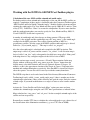
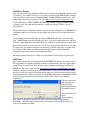
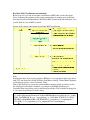
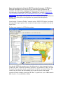
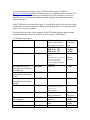
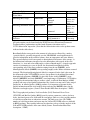
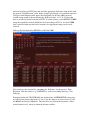
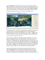
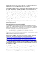
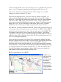
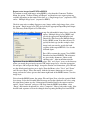
ILWIS 3.6 Open GEONETCast Toolbox Plug-in User Manual
Part 2
Version 1.
Ben Maathuis
ITC-Enschede
May 2009
Working with the ILWIS3.6 GEONETCast-Toolbox plug-in
Calculation of the sun - MSG satellite azimuth and zenith angles
For further analysis often azimuth and zenith angles of the sun and the MSG satellite are
required. Computation of these angles is facilitated under the Geonetcast Toolbox option
“MSG Satellite and Solar Zenith / Azimuth Angles”. Double click the sub menu and first
calculate the zenith angles. For Year, Month and Day specify: 2009, 06, 21 and for “Time
of day (UTC): 12.00. Press “Show” to execute the computation. If you are more familiar
with the southern hemisphere you can also specify for Year, Month and Day: 2009, 12,
21 and 12.00 UTC for the time respectively.
A number of zenith angle and derived maps are being generated. The map called
“msgzen” is the original satellite zenith angle map, the “msg_zenres” is the zenith angle
resampled to the MSG projection. These angles remain constant as MSG is a
geostationary satellite. Also the secant of the MSG satellite zenith angle map is derived,
defined as: (1/(cos(zenith_angle)))-1 . This map is called “sec_msgzen”.
Also the solar zenith angle is calculated and resampled to the MSG projection. This
output map is called: sol_zenres and the secant is “sec_solzen”. A sun elevation map is
derived, called “sun_elev” and is subsequently classified into a map called “illum_cond”,
indicating when it is day, twilight or night over the field of view of MSG.
Open the various maps created, you can use a “Pseudo” Representation. In the map
display window of the map called: msg_zenres press the “Layers” button from the
display menu, select Add Graticule and select as Graticule distance 23 degree, 26
minutes, as this is the approximate location of the Tropic of Cancer / Capricorn in the
northern and southern hemisphere respectively. Note that MSG is situated at 0 degree
above the equator. You can also add a vector layer with the country boundaries.
The ILWIS script that is used can be found in the Ilwis directory\Extensions\GeonetcastToolbox\angle\ and is called: “create_zenith_angle_maps” (there is another one for the
azimuth angle calculations). Move to this directory and open the script. Study the content
of both scripts. If you make modifications to a script it is better to store it under another
name!
Activate the “Create Satellite and Solar Angle Maps” option once more and now
calculate the Azimuth angles using the same UTC time specifications as indicted before.
Maps calculated are “msg_azres” and “sol_azres” for the resampled azimuth angles of the
satellite and sun respectively.
Eventually use another UTC time to calculate the solar zenith angle to get a better idea of
the classification of the illumination conditions (e.g. use a UTC time of 20.00).
MODIS Fire Product
This is the most basic fire product in which active fires and other thermal anomalies, such
as volcanoes, are identified. The Level 2 product is defined in the MODIS orbit geometry
(Terra satellite) covering an area of approximately 2340 by 2030 km in the across- and
along-track directions, respectively (see also: http://modis-fire.umd.edu/products.asp).
Typical filename is: MOD14.P2009150.2050.hdf.gz (MOD14.Pyyyyddd.hhmm.HDF4.
gz compressed). Note that the day number is Julian day. About 270 files / day are
disseminated.
Check in the archive, within the respective sub-directory (within ITC e.g. Z:\MODIS) the
availability of the data. Note the year and Julian date of the day of fire data you want to
import.
Open from the Geonetcast Toolbox the option “MODIS Fire Product” and sub menu
item: “MODIS Aggregated Fire Product per Day”. Specify the appropriate year and Day
Number. Check if the input and output directory settings are correct and press show. Note
that all files for that given day are processed. If fire vectors are present in the source data
the shape files are extracted and these are imported as ILWIS vector files, together with
an associated table. For more information on the table entries, check the product
description as provided on the website indicated above.
The import routine takes quite a while as a large number of files need to be processed.
MPE Direct
This routine extracts the data directly from the EUMETSAT website. So in order to run
this application the computer should be connected to the internet. The Java Applet that is
executed can be found in the Ilwis directory under: \Extensions\Geonetcast-Toolbox\
MPEdirect. The data is copied from: http://oiswww.eumetsat.org/SDDI/html/ grib.html.
From the Geonetcast Toolbox the option “MPE Direct” can be selected and if the output
directory is correctly specified the show button can be pressed to execute the processing.
Again note that these routines take time, for the MPE product derived from MSG, 96 files
have to be copied, imported and processed; for Meteosat-7 there are 48 products
respectively.
If the import process
takes too long you
can abort it by
closing the Windows
Command window.
Open a rainfall map,
use as
“Representation “
mpe_single, in the display window also add a vector layer showing the country
boundaries. Check the results; note that the values indicate the rainfall in mm over a
period of 15 minutes for MSG.
Real time MSG Visualization and animation.
Before you start a session on real time visualization of MSG take a look at the figure
below, indicating the structure of the various routines that are running once an instance
from the Geonetcast Toolbox Menu “Real Time MSG Visualization and Animation” for a
specific field of view of MSG is started.
Layout of the various components for real time MSG visualization
Note:
Format clock time of processing computer: HH:mm:ss, use appropriate time zone (offset
with UTC and local time) (From Windows Start Menu: Settings, Control Panel, Regional
and Language Options, select Customize, Time).
Source data directory in assumed in year\month\day structure. If this is not the case the
file simplegeo.bat should be modified, see example of the MSG Data Retriever
Command Line string below used for the European window. The N should be changed to
Y (see arrow for position of N in the string).
%st_ilwdir%\Extensions\Geonetcast-Toolbox\MSGDataRetriever\gdalwarp.exe --config
GDAL_CACHEMAX 30 -t_srs "+proj=latlong" -te -10.613668 35.265211 13.548728
59.013056 -tr 0.04300 0.04300 -of ILWIS MSG(%st_inputdrive%\,%workingdate%,
(1,2,3),N,B,1,1) %st_outputdrive%\%st_outputpath%\vis%workingtime%
To get an idea of the command line string that is generated by the Meteosat Second
Generation Data Retriever, open from the Geonetcast Toolbox menu, the option
“Geostationary MSG HRIT” and “MSG HRIT”. Select the various import parameters
from the menu and press the option: “Show command line”. The settings from this
command line can be copied into the batch file “simplegeo.bat” if you want to visualize
another window, but the projection “latlong” with a pixel size of 0.043 can be
maintained.
Currently from the Geonetcast Toolbox menu, using the option: “Real Time MSG
Visualization and Animation” a selection can be made of a number of standard windows.
If one of the windows is selected check the
settings of the input and output directories
and press show. In the Windows Command
window all kind of settings are performed
and in the end you are requested to provide
your password to access the file server.
Provide your password in the Command
Window and press enter. The Command Window closes and you can also close ILWIS as
the visualization is started based upon a Scheduled Task instance depending on the
system’s clock time.
To see if the Scheduled Task is created, select from Windows Start Menu: Settings,
Control Panel, Scheduled Tasks. The Task “MSG_visual” will appear. Note the
“Schedule” and the “Next Run Time”. Double click the Task “MSG_visual” and inspect
the other settings as well. Note the batch file that is executed: Run = st_msg”region”.bat
(see also the overview provided above).
If the application is left undisturbed every 15 minutes a new instance of an import
sequence is executed and all images are visualized on the screen. Activate the display
window showing the imported MSG image. To do so click with the left hand mouse
button over the image. Now you can use the scroll bar of the mouse to see the images that
have been visualized before.
To stop an instance of “Real Time MSG Visualization and Animation” select from this
menu the option “Stop Animation” and type “Y” in the Command Window. The
Scheduled Task is than being deleted from the Tasks Manager.
Import of products derived from the SPOT Vegetation Instrument: VGT4Africa
Within the GEONETCast data stream also non-meteorological organizations can
contribute. Check the listing of multicast channels to see what other data providers do
disseminate their data through EUMETCast – GEONETCast (available at: http://www.
eumetsat.int/Home/Main/What_We_Do/EUMETCast/Reception_Station_Setup/index.htm). An example is the products that are disseminated through the VGT4Africa
initiative. On a 10 day basis various products are generated and subsequently
disseminated.
Open from the “Geonetcast Toolbox” menu the option: “SPOT VGT4 Africa” and check
for yourself the import options of the various data sources that are available. See also the
figure below.
Toolbox menu structure for VGT4Africa products
Note that the VGT4Africa products are a decadal product, in order to import the various
products the “Date” format here should be specified as: yyyymmdecdec, where dec stand
for decade. There are three decades, specified as 01, 11 and 21, for the first 10 days, the
second series of 10 days and the remaining days for the last decade of the month
respectively. In the example given above the “Date” is specified as: year = 2009, month =
May, decade = 11 (second decade of May).
A lot of information is provided on the VGT4Africa Home page, available at:
http://www.vgt4africa.org. From the Homepage menu, select Documents and under User
Guides download the VGT4Africa user manual and save this document to your local
harddisk. Also read before you continue from this webpage the product sheets for the
various data types.
In the VGT4Africa user manual from page 97 onward the details are given for the various
products that are routinely produced. When importing the products it is assumed that this
reference is used prior to import.
The table below provides a short summary of the VGT4Africa product import routines
available within the Geonetcast Toolbox, under the option “VGT4 Africa”.
VGT4Africa import details
Name product
Abbreviation
Albedo Error Budget
ALBE
Albedo Quality
ALBQ
Files created upon
import (all file names
end with: yyyymmdecdec)
ERR_bbdhr
ERR_bbdhr_NIR
ERR_bbdhr_VIS
lmk (land cover map of GLC2000
classes)
sma (Status Map for Visible, Near
Infrared and total broadband
directional hemispherical
reflectance, BBDHRT, BBDHRN
Broadband directional
hemispherical reflectance –
Near Infrared
Broadband directional
hemispherical reflectance –
Total
Broadband directional
hemispherical reflectance –
Visible
BioGeo Quality
Bitwise
encoded
BBDHRN
and BBDHRV)
bbdhr_nir
* 0.001
BBDHRT
bbdhrt
* 0.001
BBDHRV
bbdhr_vis
* 0.001
BIOQ
nmod (dataset gives the number
of valid observations during the
value
Dry Matter Productivity
DMP
Fraction of Surface covered
by Vegetation
Leaf Area Index
FCOVER
Normalized Difference
Calibration
coefficients
used
* 0.0001
* 0.0001
* 0.0001
Class map
LAI
NDVI
synthesis period)
lmk and sma
dmpyyyymmdecdecv
dmpyyyymmdecdeccl
fcover
errfcover
lai
errlai
ndvi
* 0.01
Class map
* 0.004
* 0.004
* 0.033333333
* 0.005
*0.004-0.1
Vegetation Index
Normalized Difference
Water Index
Phenology Key Stages
NDWI
ndwi
*0.008-1
PHENOKS
phhalf
phlength
phstart
number of
dekads, since
January 1st,
1980
number of
dekads, since
January 1st,
1980
Phenology Maximum NDVI PHENOMAX
phmax
phmaxval
Small Water Bodies
Vegetation Productivity
Indicator
SWB
VPI
swb
vpiyyyymmdecdecv
vpiyyyymmdecdecc
*0.004-0.1
Class map
Value %
Class map
All batch routines can be found under the ILWIS directory \Extensions\GeonetcastToolbox\toolbox_batchroutines and the batch filename convention used is:
VGT4”abbreviation”import.bat. (Note that the Abbreviation refers to the product names
indicated in the table above).
Broadband albedo corresponds to the amount of solar energy reflected by a surface
(spectral albedo), spectrally integrated over the 300-3000 nm wavelength domain. It
provides information on the radiative balance, thus on temperature and water balance.
The spectral albedo in itself corresponds to hemispherical reflectance of the canopy, i.e.
the bidirectional reflectance integrated over the hemisphere with regards of the view
directions (i.e. view and solar zenith angles, relative azimuth angles). A simple approach
consists in estimating two sorts of albedo: the directional-hemispherical albedo
corresponding only to the direct radiation coming from the sun (BBDHR), and a
bihemispherical albedo (BBBHR) corresponding roughly to the diffuse radiation assumed
isotropic. The directional hemispherical albedo is computed for the local solar noon. In
the framework of the VGT4AFRICA project, data products for broadband directional
hemispherical reflectance (BBDHR) are provided for the visible (BBDHRV), near
infrared (BBDHRN) and total (BBDHRT) wavelength ranges. Furthermore, VGT4Africa
also supplies the uncertainty budgets on these values, in Albedo Error Budget (ALBE)
products and some related quality information, like a land cover map and a status map of
quality bits, in Albedo Quality (ALBQ) products. It is important to account for this
quality information and the error budgets when analysing the BBDHR values for the
different wavelength regions. (Source: From Product Meta Data description; *.XML)
The 3 biogeophysical products, Leaf Area Index (LAI), Fractional Green Cover
(FCOVER) and BioGeo Quality (BIOQ) provide various parameters, such as leaf area
index, fractional green cover, both with an error budget, land cover class and the number
of valid observations that are taken into account. The land cover class (GLC2000),
number of valid observations and status map for LAI and FCOVER values are included
in BIOQ products. These quality indicators are therefore to be used in the analysis of the
LAI and FCOVER products of the same dekad (Source: From Product Meta Data
description; *.XML).
The 3 Phenological products, Key Stages, Maximum NDVI and Monitoring provide
various phenological parameters, such as the start date of the detected growing season,
the date of half senescence, the season length, which are included in Phenology Key
Stages (PHENOKS) products. The maximum NDVI (Normalized Difference Vegetation
Index) value observed during the season and the date it was observed on can be found in
the Phenology Maximum NDVI (PHENOMAX) product of the same 10-day period and
indicators of probable start of season and other monitoring parameters can be found in the
Phenology Monitoring (PHENOMON) product. So, it is important to view the 3
Phenology products, PHENOKS, PHENOMAX and PHENOMON of the same dekad
together. To compute all these seasonal parameters, the phenology production takes into
account 54 dekads of SPOT-VEGETATION NDVI, including the current one, which
represent 1.5 years of data in total. The PHENOMON product is currently not distributed
via GEONETCast (Source: From Product Meta Data description; *.XML).
Import a number of products from VGT4Africa. Select from the Geonetcast Toolbox
menu, the option “VGT4 Africa” and retrieve some of the products. Check in the archive
which data is available before you start the import (e.g. Z:\VGT4Africa). Note that for a
number of products standard colour representations are available, like NDVI, LAI,
FCover. The class maps can be visualized using the default representation. When
visualizing the imported products also add a layer showing the country boundaries. In the
ILWIS directory \Extensions\Geonetcast-Toolbox\util\maps you will also find a vector
file only showing the African countries. This file can be copied to the active working
directory as well (use the ILWIS “copy object to” option!).
Upon import consult the product description provided in the VGT4Africa User Manual
for a more in depth discussion.
Using the Command Line History from the main ILWIS menu
ILWIS keeps a track of the last series of operations that have been executed. This
command line history is available when clicking the drop down button on the right side
of the command line under the main ILWIS menu. See also the figure below.
Access to the command history
If you quickly want to repeat import of an identical product but of a different time it is
much more convenient to simply change the time tag instead of going through the whole
menu.
An example of a command line syntax generated for the CLM import for 200906021200
is given below:
!C:\Ilwis36\Extensions\Geonetcast-Toolbox\toolbox_batchroutines\clmimport.bat 200906021200
Z: MPEF\2009\06\02 D: test_geon1 C:\Ilwis36\Extensions\Geonetcast-Toolbox\GDAL\bin
C:\Ilwis36 C:\Ilwis36\Extensions\Geonetcast-Toolbox\util
The only change that needs to be applied to import the product that is available 15
minutes later is the time stamp (now 200906021215).
!C:\Ilwis36\Extensions\Geonetcast-Toolbox\toolbox_batchroutines\clmimport.bat 200906021215
Z: MPEF\2009\06\02 D: test_geon1 C:\Ilwis36\Extensions\Geonetcast-Toolbox\GDAL\bin
C:\Ilwis36 C:\Ilwis36\Extensions\Geonetcast-Toolbox\util
You can press the command line history button and select the relevant import command,
change the time and press enter. A new instance of an import is executed for the new time
stamp given.
Try to import a later instance of a product using the command line history. First use the
menu option to import a product and note the creation of the string in the command line
when executing the operation. In a second step modify the “Date” portion of the string
from the command line history and execute a second instance of an import of a similar
product.
You can take the CLM under the “MPEF” menu. This product has a temporal frequency
of 15 minutes.
Using the Geonetcast Toolbox under ILWIS 3.6 Open with external freeware tools
Not all data import routines to use data / products that are provided through
GEONETCast need to be developed under ILWIS as a number of other freeware routines
are already available that have the capability to process certain data streams. Furthermore
other free software tools are widely used for capacity building within other disciplines,
like the use of BILKO for the marine RS society. It was considered more important to
develop efficient import or export routines, so existing capabilities of these freeware tools
can be fully utilized.
Within GEONETCast data is disseminated that is recorded by the Jason-2 altimeter
instrument and those from various sensors recorded by METOP-A. Further details are
provided how, once the processing is completed by these freeware tools, the data can be
imported into ILWIS. Also export routines are described how to transfer the results
obtained by ILWIS can be transferred to BILKO.
Processing of METOP-AVHRR/3 data using SatScape and VISAT-BEAM
EPS formatted AVHRR/3 data is disseminated in chunks of 3 minutes of recording by
GEONETCast. The filename convention uses the year, month, day, begin and end time of
recording. Sample filename is specified below:
AVHR_xxx_1B_M02_20070925072803Z_20070925073103Z_N_O_20070925090937Z
The time difference between the first date-time string and the second one is 3 minutes
(scanning from 07:28:03 to 07:31:03. Problem is that over a specific area one needs to
know when the satellite was passing over. In order to determine the time of overpass of
METOP over a certain latitude / longitude position use can be made of SatScape.
Download and install SatScape. The references are given in the document: “Other useful
software tools”. After installation start the application. From the SatScape launch pad,
note the local and UTC time. Select “Settings” and from the SatScape Settings Menu
select “Locations”. Specify in the lower part of the menu the location name and latitude /
longitude of this location. Press the “Use as Primary” button on the lower left (the
location settings will be transferred to the upper part of the menu). Save the setting.
Subsequently move to the sub menu “Groups” and from the Satellite Groups, select the
Group: weather. Scroll through the list and select METOP-A. On the right side of the
listing activate the option: Favourite. Note that the selected satellite is moving to the top
of the satellites group list.
Move to the Main tab under the SatScape Settings menu and Save all settings.
In the SatScape Launch Pad select the option: Pass Predictions. From the calendar specify
the year / month / day you would like to select to determine the time of satellite overpass
for your specific location. Select from “This Satellite” drop down list METOP-A and
press the GO button. In the table that is subsequently generated the overpasses of the
satellite is given. You can use the “Peak” local time to get an idea of the best overpass
images. If interested in images of the morning overpass, first note the time offset
between local time and UTC time and select the appropriate local time using the file with
the greatest “Peak Elevation” value. In the example given below, for a location situated at
52 degree North Latitude and 6 degree East Longitude, for 01-June-2009, the most
suitable image would be the one having the “Peak local time” of 12:31:18. Note that
there is an offset between local time and UTC of minus 2 hours, so the METOP AVHRR
image that should be selected should have been recording at 10:31:18. As the AVHRR
data is provided with start and end of scan time, the appropriate image can be easily
selected.
SatScape Pass Prediction for METOP-A of 01-June-2009
Select and copy the relevant file, containing the “Peak time” for the greatest “Peak
Elevation” from the archive (e.g. Z:\METOP) to your local working directory. Close
SatScape.
Download and install VISAT-BEAM, also download the AVHRR METOP reader plugin, called: beam-metop-avhrr-reader-1.3.jar. Copy this plug-in (at least version 1.3) into
the BEAM sub directory \Modules. The references are given in the document: “Other
useful software tools” where to obtain the freeware utilities.
Open VISAT-BEAM, select from the main menu the option File, Import and Import
Metop-AVHRR/3 Level-1b Product. Browse to your active working directory and double
click the selected file that you have copied from the archive before. The file name now
appears in the product view. To get an idea of the area recorded by METOP-AVHRR/3
select from the main menu, View, Tool Windows and World Map. The field of view of
the specific recording is indicated over a world map. See also figure below.
Worldmap showing extent of AVHRR/3 image selected
If satisfied with the area covered by the selected image you can display the image. Right
click with the mouse over the filename in the Product View and from the context
sensitive menu select the option: “Open RGB Image View”. From the “VISAT – Select
RGB-Image Channels, select from the drop down list under “Profile”: AVHRR/3 L1b –
3a,2,1,Day and press OK. You can zoom in and out using the navigator available at the
top left portion of the image display window.
Once more click on the file name of the imported image in the Product View, when
selected it will appear blue. Now select from the main menu the option: “Tools”, “Map
Projection”. Change the “Name” to an appropriate name, e.g. avhrr_utm and under
“Projection” select UTM Automatic. Press OK. In the Product View window a new item
is now added (e.g. called avhrr_utm). Right click with the mouse over the filename in the
Product View and from the context sensitive menu select the option: “Open RGB Image
View”. From the “VISAT – Select RGB-Image Channels, select from the drop down list
under “Profile”: AVHRR/3 L1b – 3a,2,1,Day and press OK. You can zoom in and out
using the navigator available at the top left portion of the image display window.
Once more click on the file name of the projected image in the Product View, when
selected it will appear blue. Now select from the main menu the option: “Export”,
“Export GeoTIFF Product”. Select an appropriate output directory and press “Export
Product”. This will take some time as all bands are exported. Note from the Products
View the various bands that are available (radiance, reflectance, temperature, angles, etc).
Note the band number for reflec_1, reflec_2 and reflec_3a as you will use these later in
ILWIS. You can close VISAT-BEAM when the export is completed.
Open ILWIS 3.6 with the Geonetcast Toolbox installed and select from the toolbox menu
the option: “Import METOP – AVHRR/3 from BEAM”. Specify the appropriate input
file / directory and output file / directory. Move to the specified output directory when the
import is completed. Double click the map list created, the name you specified as the
output file when importing the image. From the map display options menu select the
band numbers that represent: reflec_1 for the Blue Band, reflec_2 for the Green Band and
reflec_3a for the Red Band and press OK (most likely band numbers 6, 7, 8
respectively!!). There is no need to change the default stretch values. Add a vector file
showing the country boundaries to the map display (using the option info off) and check
the geometric properties. Move the mouse, with the left mouse button pressed over the
map display. Check the values obtained.
Also display the other imported image layers and note what these represent as well as
their radiometric properties.
Import of JASON-2 processing results from BRAT
The Basic Radar Altimetry Toolbox is an excellent utility to perform the processing of
altimetry data. The processed altimetry data that is recorded by the JASON-2 instrument
is disseminated via GEONETCast. Check on the file server the data that is available (e.g.
Z:\JASON). Look for the data having a file name convention as:
JA2_OPN_2PcS033_194_20090601_212231_20090601_231853.bz2
Copy a selected set of JA2_OPN files to your local harddisk. Before you can use the data
in BRAT, make sure that the files are decompressed.
Download and install BRAT. The references are given in the document: “Other useful
software tools”. Also consult the information as provided by EUMETSAT, at:
(http://www.eumetsat.int/Home/Main/What_We_Do/Satellites/Jason/index.htm?l=en)
and download the OSTM / Jason-2 Products Handbook, which is available at:
(http://www.eumetsat.int/Home/Main/What_We_Do/Satellites/Jason/Services/?l=en)
This document is providing more information about the file name convention that is used,
etc. Below a short summary is provided of the main steps in BRAT. For more elaborate
exercise material consult the Reference Guide and Training manuals that are provided at
the download site of BRAT.
Open BRAT and create a new Workspace and save it. From the menu, select “Datasets”
and create a new one. You can give it a relevant name, e.g. Jason_OGDR, select the
option “Add Files” and add all decompressed Jason-2 files.
Select from the menu “Operations” and create a new operation, provide it with an
operation name (e.g. Jason_OGDR). Active your current dataset under the heading
“Datasets”. In the “Fields” below, select “lon (degrees_east)”, right click your mouse and
select: “set as X”, Repeat this procedure for “lat (degrees_north)” and “set as Y”.
Now note the “Resolution and filter information”, default settings are for a global
definition at a spatial resolution of 1/3 degree.
Now under the “Data Expressions” you will see that X is defined as longitude, Y is
defined as latitude. Right click with the mouse on the “Data” field and “Insert Empty
Expression”. Again right click on the created “Expression” and select “Insert a Formula”.
Now you can select: SSH_Jason1_GdrA, uncheck “as alias” and press OK. The full
expression is now provided. Modify the first parameter “altitude” in the Expression and
change this to “alt”. You can eventually press the option “Check syntax”. After this
modification you should not get a warning message when the syntax is checked.
Press “Execute” to start the calculation of the SSH_Jason1_GdrA operation. If you get an
error message at the start of the processing, save your work, exit BRAT and Start BRAT
again and execute the operation once more. You can display your results in BRAT. This
is not further described here as you are now going to use the “Export” option. In the
“Operations” menu, press “Export”. Note that for import in ILWIS a Global resolution is
required (X from -180 to 180 and for Y from -90 to 90). The resolution (Step) can be 1/3,
1/5, 1/7, 1/9 of a degree respectively.
Specify that the export format is NetCdf and select an appropriate filename and output
directory in the Export menu. Press OK to execute the export. Open ILWIS, and from the
Geonetcast Toolbox select the option “Import Jason-2 from BRAT”. Select the
appropriate input file and specify an output file. Also specify the appropriate resolution,
1/3 of a degree is 3, etc. Press OK to execute the import. Display the resulting map using
a pseudo representation and eventually stretch the map, e.g. from -50 to 50. Also add a
vector file showing the country boundaries. Browse with the cursor, pressing the left
mouse button over the map and check the resulting values.
BRAT exported altimetry data in ILWIS
In BRAT many
other processing
options are
available, check
the training
material that is
provided to get a
better overview
of the capabilities
of this freeware
altimetry toolbox.
Export raster images from ILWIS to BILKO
To continue to work with images using BILKO, select from the Geonetcast Toolbox
Menu, the option “Toolbox Settings and Export” and from here two export options are
available depending on the nature of the data: as a “Single image layer” (exported as TIF)
and as “Multiple image layers” (exported as HDF4).
Check in your active working directory a map / image with a single image layer, select
the option “ Single image layer (TIF) and specify the appropriate Input Map and Output
file / Directory in the Export to GeoTiff menu.
Check in your active working directory an map list with multiple image layers, select the
option “ Multiple image layers (HDF4) and
specify the appropriate Input MapList and
Output file / Directory in the Multiple Image
Layers (HDF4) menu. Note that you need to
specify the data type (in this example a byte
image) and you can also specify the band
sequence in the output HDF file. See also the
left hand figure.
Press OK to execute the export. Close ILWIS.
Download and install BILKO. The references
are given in the document: “Other useful
software tools”. After installation start the
application. From the BILKO main menu select “File” and “Open”, move to the directory
where you stored the previously exported TIF single image layer, select the appropriate
file and press OK to Open the Image. Accept the window size dimensions, press OK and
use the default stretch option, press Apply. From the Menu, select “View” and “Zoom”
and “Preserve Shape”. Move the mouse, with the left mouse button pressed over the
image and note the values given at the bottom right hand of the BILKO menu. Close the
image layer.
Select from the BILKO menu, the option: File and Open. Now select the exported Multi
layer image. Select the Scientific Data Directory and on the right hand side select, using
the right mouse button over the 3-dimensional Scientific Dataset, the context sensitive
option: “Open Connected” and press OK. Now from the BILKO main Menu, select
“Image” and from the dropdown list, select “Composite”. Have a look at the results, Note
that the band sequence used can be changed when exporting the Map List from ILWIS.