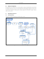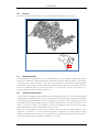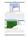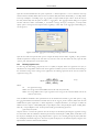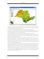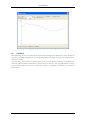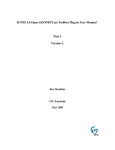
1
APPLICATION MANUAL
5.
ASSESSING VEGETATION COVERAGE AT THE SAO
PAULO STATE SCALE: “A TOOL FOR AIDING THE
DECISION MAKING PROCESS”
By: Fabio Enrique Torresan1
5.1.
Relevance and importance of the application
The availability of reliable information of the agricultural production data is increasingly a fundamental demand in
the decision making process, both for national and international scenarios (Pino, 1999; Epiphanio et al., 2002;
Dronin & Bellinger, 2005; Epiphanio, 2007; Castillejo-González et al., 2009).
The operational methodology currently applied to perform agricultural forecasting in Brazil is done through
extensive, prolonged, expensive and subjective surveys based on the opinion of technical agents involved in the
agricultural segment (Instituto Brasileiro de Geografia e Estatística, 2002) and therefore the analysis is biased, due to
the errors and uncertainties involved and renders this methodology less practical.
Therefore, an increasing demand is observed for agricultural forecasts derived from remote sensing data, which allow
faster results, with higher accuracy and lower costs than the traditional techniques (Food and Agriculture
Organization of the United Nations, 1998; Prasad, 2006).
In the same way, there is also a great gap with respect to information about the degree of conservation of the
remaining natural vegetation coverage. Global demand for agricultural products is now a major driver of cropland
and pasture expansion across much of the developing world. Whether these new agricultural lands replace forests,
degraded forests or grasslands greatly influences the environment. While the general pattern is known, there is still
no definitive quantification of these land cover changes (Gibbs, 2010).
Conservation of biodiversity within managed landscapes calls for a strategy that includes increasing the conservation
value of the agricultural matrix both in terms of providing viable habitat for forest-dependent species, as well as
increasing connectivity between protected areas and forest fragments (DeClerck et all, 2010).
The identification, mapping and monitoring of the land use changes is an important tool to support decision making,
both for public managers and for agribusiness investors. At the same time, recovery and utilization of degraded areas
and restoration of native vegetation could prevent the advance of deforestation in areas of agricultural expansion.
In this context, the Vegetation instrument on board the SPOT satellite deliver measurements specifically tailored to
monitor land surface properties with a frequency of about once a day on a global basis and at a spatial resolution of
one kilometer (in fact 5 times over 6 days at the equator, once a day at 30° latitude, and twice a day at latitudes higher
than 60°). These characteristics allow monitoring large extents of land in a continuous way.
1 Embrapa Satellite Monitoring, Av. Soldado Passarinho, 303 - Fazenda Chapadão CEP 13070-115 - Campinas, SP, Brasil
(www.cnpm.embrapa.br), email
[email protected]
55
APPLICATION MANUAL
5.2.
Objective of the application
The main objective for this application is to assess the vegetation coverage at the municipalities from the Sao Paulo
State (Brazil) using data from a temporal set of S10 NDVI images, acquired by SPOT Vegetation instrument, which
are available from the DevCoCast project. After the validation of this methodological approach in a near future, it
would be useful to implement a monitoring system using the vegetation cover and make it available to decision
makers and for the society.
5.3.
Methodology and study area
5.3.1.
Methodology adopted
A flow chart of the followed methodology is presented in figure 5.1 below.
S10 NDVI temporal series from SPOT Vegetation
Step 1
Maximum Value
Composition
Step 2
one MapList
for each
month
Step 3
Digital Vector Data (shapefile)
one NDVI map
for each month
Attribute Table
Step 5
Step 4
one MapList
with 24 NDVI mensal maps
Vector Map of Sao Paulo municipalities boundaries
Step 7
Step 6
NDVI sub maps limited
by São Paulo State
boundaries
Step 9
Step 8
Output Crosstable
Vegetation Coverage
Maps for each month
Step 10
Average Vegetation Coverage
Maps for each month and for each municipality
Figure 5.1 Flowchart of the adopted methodology
56
Raster Map of Sao Paulo municipalities boundaries
APPLICATION MANUAL
5.3.2.
Study Area
The study area covers the São Paulo State, Brazil, consisting of 645 municipalities, see also figure 5.2.
Figure 5.2 Sao Paulo State with the municipal boundaries and its location in Brazil
5.4.
Data pre-processing
For this application, a temporal data set is used of S10 NDVI images. The 10-day SPOT Vegetation S10 synthesis
products are a combination of daily atmospherically corrected data of all VEGETATION segments (measurements)
of the given decade (10-day period) into a single image using the Maximum Value Composite (MVC) algorithm,
which selects the pixels with the best ground reflectance values (Bartholomé, 2006). Here a temporal data set is used
from the years 2008 and 2009. Not all time steps need to be pre-processed, as example of the necessary preprocessing required, the month of December 2009 is used.
5.4.1.
Importing the S10 NDVI images
A temporal series of S10 NDVI images derived from the SPOT Vegetation Instrument, for the years 2008 and 2009,
available within the GEONETCast data stream should be imported into the Integrated Land and Water Information
System (ILWIS), using the GEONETCast Toolbox (see figure 5.3). Ensure that you have unzipped the exercise data,
open ILWIS and move using the ILWIS navigator to this active working directory. You will note that there is a sub
directory “gnc_data”. The directory is containing the raw data from GEONETCast-DevCoCast. Once close ILWIS
and Open ILWIS again to ensure that the directory settings are correct.
Ensure that the GEONETCast toolbox plug-in is installed, open from the main ILWIS menu the option
“Operations => Geonetcast” => “toolbox”, now select the option “Configuration” => Folders”. Specify the folder
settings for “SPOT VGT4 Latin America”, set the appropriate input and output folders, note that the input folder is
your active working directory and add here the sub-directory “\gcn_data”.
57
APPLICATION MANUAL
From the ILWIS Main Menu, import the NDVI images for the 3 decades of December for the year 2009, select
from the ILWIS menu: “Operations => Geonetcast => Toolbox => SPOT VGT Products => SPOT VGT Latin
America => NDVI”. Use as “Date” stamps: “20091201”, “20091211” and “20091221” respectively.
Figure 5.3 Importing S10 NDVI images using the Geonetcast Toolbox plug-in
Open the imported maps “ndvi20091201”, “ndvi20091211” and “ndvi20091221”, use as Representation “NDVI1”,
browse with the left mouse cursor pressed over the map and inspect the values. Note that also a status map, (*_SM)
is created. This status map is going to be applied to select only those pixels that meet the following criteria: cloud
free, land pixel and having good radiometry in the red and near infra red channels. For further explanation on the
procedure, see also Maathuis et al (2011). Type the following map calculation formula on the command line in the
main ILWIS menu:
Status_ok:=iff((((ndvi20091201_SM div 1)mod 2)+(( ndvi20091201_SM div 2)mod 2)=0) and
(((ndvi20091201_SM div 8)mod 2)+((ndvi20091201_SM div 32)mod 2)+((ndvi20091201_SM div 64)mod
2)=3),1,0)
Leave all other options as default and execute the operation. Inspect the resulting map and now apply the mask,
showing the pixels meeting the selection criteria, to the NDVI map by entering the following map calculation
statement on the command line in the main ILWIS menu:
ndvi_ok20091201:=iff(Status_ok=1,ndvi20091201,?)
Again use all other settings as default and execute the operation, check the results, use as Representation “NDVI1”.
Repeat this procedure for the other two decades as well. Use the command line history from the main ILWIS menu
and change the date string portions!
5.4.2.
Creating a Map List for the imported NDVI images
Create one map list for each month, with the three decades from its corresponding month (see figure 5.4). From the
ILWIS Main Menu select “File => Create => Map List” and make for the month of December 2009 a map list
consisting of the 3 corrected decadal maps “ndvi_ok200912*”. Specify as output map list name “122009”
58
APPLICATION MANUAL
Figure 5.4 Example Map List created with the three decades from December 2009
5.4.3.
Extracting the Monthly Maximum Value Composition
From the map list created, the three NDVI images will be merged into another raster map, resulting in the maximum
NDVI value for each month. Right click with the mouse the map list “122009”, from the context sensitive menu
select “Statistics => Maplist Statistics”, as Statistic Function select “Maximum”, specify as output map “max200912”
and press “Show” to execute the operation. To display the map use as Representation “NDVI1” and press “OK”.
Now add the polygon file “spnovo”, select from the active map window the options “Layers => Add Layer” and
select “spnovo”. From the menu “Display Options – Polygon Map”, unselect the option “Info” and activate the
option “Boundaries Only”. The polygon boundaries are now draped over the raster NDVI map, use the “Zoom-in”
option from the active map window and select the area of interest. Next, from the active map window, select the
option “File => Open Pixel Information” and move the mouse cursor over the map to see the corresponding table
attributes. Your results should resemble those of figure 5.5.
Figure 5.5 Monthly NDVI maximum value composite with Sao Paulo State political vector map
In order to calculate the operations only for the study area it is necessary to create a “Sub map”. To create a sub map
it is necessary to select using the right mouse button the “max200912” map and choose from the context sensitive
menu the “Spatial Reference Operations => Sub Map” options. The details to select only the Sao Paulo State are
provided in figure 5.6 and press “Show” to execute the operation and display the sub map using the Representation
“NDVI1”.
59
APPLICATION MANUAL
Figure 5.6 Sub map settings to select the Sao Paulo State region
Most of the analysis in ILWIS is based on raster data. Therefore, conversion from vector to raster format (rasterize)
is often a necessary step preceding the analysis. Right-click with the mouse the polygon file “spnovo”, from the
context sensitive menu select the option “Polygon to Raster”, as Georeference select “submax2008_1” and type for
the Output Raster Map: “municipios”, press “Show” to execute the operation. Press “OK” to display the map using
the default settings. Close the map and right-click with the mouse the newly created raster map “municipios”, select
“Properties” and note that the Attribute Table “spnovo” is attached to this map. Double click with the left mouse
button the table “spnovo” to display it and inspect the content. Its content is identical to the record that is displayed
when using Pixel Information (see also figure 5.5).
5.5.
Data analysis
In order to conduct the full pre-processing chain, as indicated in chapter 5.4, for the whole time series requires a lot
of time. Therefore a full pre-processed sub set of NDVI data of the Sao Paulo region has been prepared. The
methodology used to create this time series is identical as described above. The time series NDVI maximum value
composites are provided in the map list “submax2008_2009”. Double click with the mouse the map list name, use
the option “Open as Slide Show”, select as Representation “NDVI1” and press “OK” twice to see then animated
sequence of this time series. After the content is inspected close the visualization.
5.5.1.
Statistical analysis on the NDVI values for each municipality
An important tool for data analysis in ILWIS is the Cross operation, which calculates the frequency of occurrence of
all possible combinations of two maps. The Cross operation performs an overlay of two raster maps by comparing
pixels at the same positions in both maps and keeping track of all the combinations that occur between the values or
classes in both maps. The input maps used in a Cross operation should be raster maps that have the same
georeference. During the Cross operation, combinations of class names, identifiers or values of pixels in both maps
are listed, the number of pixels occurring as this combination is counted, and the areas of the combinations are
calculated. The results are stored in an output cross table and optionally an output cross-map can be created. The
output cross-table and the output cross-map obtain an ID domain with the same name as the output cross-table. The
domain contains items, which are combinations of the class names, IDs, group names or values of the first input
map and those of the second input map.
You are going to cross a raster map with an identifier domain called “municipios” (created before, containing the
municipal areas of the State of Sao Paulo) and the NDVI maximum monthly value map for each month of the years
2008 and 2009. The result is a large cross-table which contains the combinations of the municipality names - codes
and the number of pixels with a certain NDVI value.
60
APPLICATION MANUAL
Open from the main ILWIS menu the option “Operations => Raster Operations => Cross”. Select the raster map
with the maximum monthly NDVI values for the 1st month of 2008, here called “submax2008_1” as 1st Map. Select
raster map “municipios” as 2nd Map. Type “avg_01_2008” as Output Table and press “Show”. From the menu of
the newly created table, select the option “Columns => Aggregation”. The Aggregate Column dialog box is opened
and now select the Column: “submax2008_1”, as Function “Average” Group by “municipios”, as Output Table
specify “spnovo” and type for the Output Column “avg2008_1”. Click “OK” in the Aggregate Column dialog box,
see also figure 5.7.
Figure 5.7 Column aggregation and adding resulting column to external table
Open the cross table and open the table “spnovo”. Inspect the newly created column “avg2008_1”. This procedure
should be repeated for all maps in the time series. If you do not want to do this another 23 times, open the table
“spnovo_ndvi” and inspect the content of this table.
5.5.2.
Estimating vegetation cover
For this step, the methodology proposed by Gao et al. (2006) is adopted, which uses vegetation cover (VC) to
calculate the rate of degradation and the result can be applied to establish a system for assessment and monitoring of
the environment using remote sensing. In this application, the following expression will be used to estimate the
vegetation coverage (VC):
(Eq 1)
Where:
VC
the vegetation coverage
NDVIS the average of the minimal NDVI value of the study area (here 0.192)
NDVIV the average NDVI value of pure vegetation or the average of the maximum NDVI value in the
study area (here 0.671)
Note that NDVIS and NDVIV values specified above can be obtained from the table (e.g. the table “spnovo”, using
the aggregated minimum and maximum statistical values of the 24 “avgyear_month” columns). Select from the main
ILWIS menu the option “Operations => Raster Operations => MapList Calculation”, see also figure 5.8. Select the
NDVI time series map list “submax2008_2009” as input MapList and as Output MapList specify “vc2008_2009”.
Here only “1” Input MapList is used. In the expression field, type the following expression:
((@1-0.192)/0.671)*100
and press “Show” to execute the operation. Now 24 new maps are calculated, representing the vegetation coverage
for each month. After the calculation is finished open the newly created maplist “vc2008_2009”, double click one of
the map layers and display the map using a Representation “vgcover”. See a resulting example of January 2008 with
the municipality boundaries in figure 5.9. Close the map and now display it as an animated sequence, using the same
Representation. Close the animation when finished.
61
APPLICATION MANUAL
Figure 5.8 MapList Calculation
Figure 5.9 Vegetation coverage for January 2008
Now the monthly average vegetation cover maps have to be crossed with the municipality raster map. Repeat the
same procedure as described in chapter 5.5.1 but now cross the vegetation cover maps for each month with the
raster municipality map. This will result in 24 new columns in the table “spnovo”, use as column prefix name “vc_”.
If you don’t want to repeat the procedure 24 times, open the table “spnovo_ndvi_vc” and inspect the content.
5.5.3.
Municipal Vegetation Cover maps
Having calculated the average vegetation cover per municipality in the table, this information is now going to be
spatially represented. First select, by right clicking the mouse over the raster map “municipios” the Properties Dialog
Box. Ensure that from here the Attribute Table “spnovo_ndvi_vc” is selected and press “Apply” and “OK”. Again,
right click with the mouse, the map “municipios” and select “Raster Operations => Attribute Map”, as Attribute
select the column “vc012008” and as Output Raster Map specify “muni_vc012008”, press “Show” to execute the
operation and display the resulting map using a Representation “vgcover”. The result is also given in figure 5.10.
62
APPLICATION MANUAL
Figure 5.10 Vegetation cover aggregated per municipality, Sao Paulo State, January 2008
Check the command line string from the main ILWIS menu, use the drop down icon on the right hand corner of the
command line. The expression generated to execute the operation can be adapted and a new map can be calculated.
The string that was used to calculate the attribute map is:
muni_vc012008.mpr{dom=value;vr=4.28:94.79:0.01} = MapAttribute(municipios,vc012008)
To calculate a new map the output map name needs to be changed and the attribute column. Open once more the
table and note that the attribute column for the vegetation cover of February 2008 is called “vc_fev2008”. Now
change the expression given in the command line history following:
muni_vc022008.mpr{dom=value;vr=0.00:100.00:0.01}:=MapAttribute(municipios,vc_fev2008)
Press enter (from the active command line) to execute this operation and “OK”. Keep on changing the input
attribute column and output map name to obtain a time series of 24 VC municipality aggregated maps. All command
line expressions are also presented in appendix 1.
When all 24 muni_vc* maps are created, open from the ILWIS main menu the options “File => Create =>
MapList”, specify as MapList name “muni_vc”, select all 24 muni_vc* maps and use the “>” icon to transfer them to
the right hand map listing, press “OK”. Display the newly created maplist as an animated sequence, using as
Representation “vgcover”, and press “OK” twice. In the active map window, select the option “Layers =>Add
Layer”, add the polygon file “spnovo”, from the menu “Display Options – Polygon Map”, unselect the option
“Info” and activate the option “Boundaries Only”.
Once more open the maplist “muni_vc” and display the map “muni_vc012008”. Add to this map the vector layer
showing the municipalities and use the option boundaries only for display of this vector layer. Now from the main
ILWIS menu, select “Operations => Statistics => MapList => MapList Graph” In the maplist graph window, select
as MapList “muni_vc”, use a fix stretch of 0 to 100, activate the options “Continuous” and “Always on top”.
Activate the map window showing the previously opened map layer “muni_vc012008”. Browse with the mouse
cursor over the map. Note the aggregated vegetation cover time series values in the graph window, see also figure
5.11. You can also change the maplist, e.g. use submax2008_2009 to see the maximum monthly NDVI values. Note
that you have to change the fix stretch from 0 to 1!
63
APPLICATION MANUAL
Figure 3.11 Aggregated Vegetation Cover and time series graph of a pixel
5.6.
Conclusions
This methodology needs to be validated with in-situ data. The thresholds of the NDVI values used to calculate the
vegetation cover (NDVIS and NDVIV) may be changed depending on the length of the time series available and also
on the area of interest.
This methodology can be adapted to different objectives, like crop and biomass monitoring and for biodiversity
monitoring and environmental management of protected areas. In this case, other geographical limits of analysis
need to be adopted, like the extents of a certain land use regions, the boundaries of watersheds or of parks and
protected areas.
64
APPLICATION MANUAL
REFERENCES
Bartholomé, E. (editor) (2006): VGT4Africa user manual. 1st edition. EUR 22344 EN, European Communities.
Available online in English and French at http://www.devcocast.eu/ViewContent.do?pageId=40 (last accessed on
2011-02-01).
Castillejo-González, I.L., López-Granados, F., García-Ferrer, A., Peña-Barragán, J.M., Jurado-Expósito, M., Sánchez
de la Orden, M. and González-Audicana, M. (2009): Object- and pixel-based analysis for mapping crops and their
agro-environmental associated measures using QuickBird imagery. Computers and Electronics in Agriculture, v.68, p.207215, 2009.
Dronin, N.M., Bellinger, E.G. (2005): Climate dependence and food problems in Russia, 1900-1990: the interaction
of climate and agricultural policy and their effect on food problems. Budapest, Hungary. Central European
University Press, 2005. 366p.
Epiphanio, J.C.N., Luiz, A.J.B., Formaggio, A.R. (2002): Estimativa de áreas agrícolas municipais, utilizando sistema
de amostragem simples sobre imagens de satélite. Bragantia, v.61, p.187-197, 2002.
Epiphanio, R.D.V. (2007): Avaliação da potencialidade das imagens MODIS na estimação da área de soja no Estado
do Mato Grosso. 2007. 89p. Dissertação (Mestrado) - Instituto Nacional de Pesquisas Espaciais, São José dos
Campos.
Fabrice A.J. DeClerck, Robin Chazdon, Karen D. Holl, Jeffrey C. Milder, Bryan Finegan, Alejandra Martinez-Salinas,
Pablo Imbach, Lindsay Canet, Zayra Ramos (2010): Biodiversity conservation in human-modified landscapes of
Mesoamerica: Past, present and future. Biological Conservation. Volume 143, Issue 10, Conserving complexity: Global
change and community-scale interactions. Tropical forest biodiversity in a human-modified world: a multi-region
assessment. October 2010. Pages 2301-2313. ISSN 0006-3207, DOI: 10.1016/j.biocon.2010.03.026.
Gao, Q., Li, Y., Wan, Y., Lin, E., Siong, W., Jiangcun, W., Wang, B. and Li, W. (2006): Grassland degradation in
northern Tibet based on remote sensing data. J. Geographical Sciences, v. 13, n. 2, p. 165-173, 2006.
Instituto Brasileiro de Geografia e Estatística (2002): Pesquisas agropecuárias. Rio de Janeiro, Brazil. IBGE, 2002.
v.6, 96p. (Série relatórios metodológicos).
Maathuis, B., Mannaerts, C., Retsios, B., Schouwenburg, M. and Lemmens, R. (2011): GEONETCast Toolbox.
Installation, configuration and user guide of the GEONETCast Toolbox plug-in for ILWSI 3.7, XML version 1.2.
ITC. Enschede, The Netherlands. 2011. http://52north.org/downloads/earth-observation/geonetcast/toolbox
PINO, F.A. (1999): Estatísticas agrícolas para o século XXI. Agricultura em São Paulo, v.46, p.71-105, 1999.
65
APPLICATION MANUAL
APPENDIX 1
Listing op map calculation statements to compute the aggregated VC per municipality.
Type the expressions below on the command line in the main ILWIS menu to calculate the vegetation cover (VC)
for each month of the year 2008 and 2009.
muni_vc012008.mpr{dom=value;vr=0.00:100.00:0.01}:=MapAttribute(municipios,vc012008)
muni_vc022008.mpr{dom=value;vr=0.00:100.00:0.01}:=MapAttribute(municipios,vc_fev2008)
muni_vc032008.mpr{dom=value;vr=0.00:100.00:0.01}:=MapAttribute(municipios,vc_mar2008)
muni_vc042008.mpr{dom=value;vr=0.00:100.00:0.01}:=MapAttribute(municipios,vc_abr2008)
muni_vc052008.mpr{dom=value;vr=0.00:100.00:0.01}:=MapAttribute(municipios,vc_mai2008)
muni_vc062008.mpr{dom=value;vr=0.00:100.00:0.01}:=MapAttribute(municipios,vc_jun2008)
muni_vc072008.mpr{dom=value;vr=0.00:100.00:0.01}:=MapAttribute(municipios,vc_jul2008)
muni_vc082008.mpr{dom=value;vr=0.00:100.00:0.01}:=MapAttribute(municipios,vc_ago2008)
muni_vc092008.mpr{dom=value;vr=0.00:100.00:0.01}:=MapAttribute(municipios,vc_set2008)
muni_vc102008.mpr{dom=value;vr=0.00:100.00:0.01}:=MapAttribute(municipios,vc_out2008)
muni_vc112008.mpr{dom=value;vr=0.00:100.00:0.01}:=MapAttribute(municipios,vc_nov2008)
muni_vc122008.mpr{dom=value;vr=0.00:100.00:0.01}:=MapAttribute(municipios,vc_dez2008)
muni_vc012009.mpr{dom=value;vr=0.00:100.00:0.01}:=MapAttribute(municipios,vc_jan2009)
muni_vc022009.mpr{dom=value;vr=0.00:100.00:0.01}:=MapAttribute(municipios,vc_fev2009)
muni_vc032009.mpr{dom=value;vr=0.00:100.00:0.01}:=MapAttribute(municipios,vc_mar2009)
muni_vc042009.mpr{dom=value;vr=0.00:100.00:0.01}:=MapAttribute(municipios,vc_abr2009)
muni_vc052009.mpr{dom=value;vr=0.00:100.00:0.01}:=MapAttribute(municipios,vc_mai2009)
muni_vc062009.mpr{dom=value;vr=0.00:100.00:0.01}:=MapAttribute(municipios,vc_jun2009)
muni_vc072009.mpr{dom=value;vr=0.00:100.00:0.01}:=MapAttribute(municipios,vc_jul2009)
muni_vc082009.mpr{dom=value;vr=0.00:100.00:0.01}:=MapAttribute(municipios,vc_ago2009)
muni_vc092009.mpr{dom=value;vr=0.00:100.00:0.01}:=MapAttribute(municipios,vc_set2009)
muni_vc102009.mpr{dom=value;vr=0.00:100.00:0.01}:=MapAttribute(municipios,vc_out2009)
muni_vc112009.mpr{dom=value;vr=0.00:100.00:0.01}:=MapAttribute(municipios,vc_nov2009)
muni_vc122009.mpr{dom=value;vr=0.00:100.00:0.01}:=MapAttribute(municipios,vc_dez2009)
66