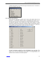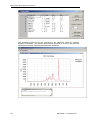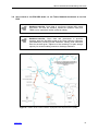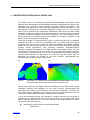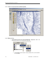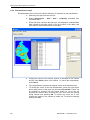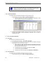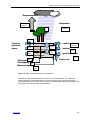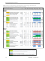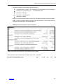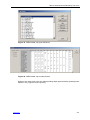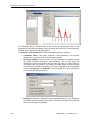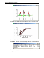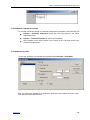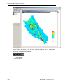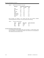
1
Mekong River Commission HBV and IWRM Watershed Modelling User Guide MRC Information and Knowledge Management Programme DMS – Detailed Modelling Support for the MRC Project December 2010 Finnish Environment Institute in association with EIA Centre of Finland Ltd. DMS-Project, Mekong River Commission DMS - Detailed Modelling Support to the MRC Project HBV and IWRM Watershed Modelling User Guide MRC Information and Knowledge Management Programme December 2010 Jorma Koponen, Hannu Lauri, Noora Veijalainen and Juha Sarkkula Finnish Environment Institute Mechelininkatu 34a 00260 Helsinki Finland Tel: +358-9-403 000 Fax: +358-9-40300 390 www.environment.fi/syke [email protected] 2 EIA Ltd. Tekniikantie 21 B 02150 Espoo Finland Tel: +358-9-7001 8680 Fax: +358-9-7001 8682 www.eia.fi [email protected] MRCS/IKMP --- December 2010 HBV and IWRM Watershed Modelling User Guide TABLE OF CONTENTS TABLE OF CONTENTS................................................................................................................... 3 1 STRUCTURE OF THE USER GUIDE ...................................................................................... 7 1.1 STRUCTURE OF CHAPTER AND INFORMATION BOXES ........................................................... 7 1.2 EXERCISES ........................................................................................................................ 8 2 IWRM MODELLING BACKGROUND ...................................................................................... 9 2.1 WHAT IS IWRM MODELING ................................................................................................. 9 2.2 HISTORICAL OVERVIEW OF THE MRC IWRM MODEL DEVELOPMENT .................................. 10 3 LUMPED HYDROLOGICAL MODELLING ............................................................................ 12 3.1 OVERVIEW OF LUMPED AND DISTRIBUTED MODELLING ....................................................... 12 3.2 NOOA EXPERIENCES OF LUMPED AND DISTRIBUTED MODELLING ....................................... 14 3.3 GENERAL PRINCIPLES OF THE LUMPED HBV MODEL .......................................................... 15 3.4 EIA HBV MODEL .............................................................................................................. 19 3.5 EIA HBV MODEL APPLICATION STEPS ............................................................................... 21 3.5.1 Install modelling software .......................................................................................... 21 3.5.2 Prepare input data into the HBV model format ......................................................... 21 3.5.3 Data preparation using the 3D model user interface ................................................ 21 3.5.4 Data preparation with the DTT (Toolbox Data Transfer Tool) using the ToolBox Knowledge Base data ............................................................................................................. 27 3.5.5 Create model application ........................................................................................... 31 3.5.6 EIA HBV model calibration ........................................................................................ 35 3.6 APPLICATION OF THE EIA HBV MODEL TO THE THEUN HINBOUN WATERSEHD IN THE LAO PDR 37 4 DISTRIBUTED HYDROLOGICAL MODELLING................................................................... 39 4.1.1 Water quality and erosion computation ..................................................................... 42 4.1.2 Input and output data................................................................................................. 43 4.1.3 Model user interface .................................................................................................. 44 5 BASICS FOR USING THE IWRM MODEL ............................................................................ 47 5.1 SOFTWARE INSTALLATION ................................................................................................ 47 5.2 FILE SYSTEM .................................................................................................................... 50 5.2.1 Model system files ..................................................................................................... 50 5.2.2 Model application files ............................................................................................... 50 5.2.3 TXD file format ........................................................................................................... 51 5.3 STARTING THE IWRM MODEL SOFTWARE ......................................................................... 53 5.3.1 Starting the software from EIAModels desktop shortcut icon ................................... 53 5.3.2 Starting the software from vmp-file............................................................................ 55 5.4 IWRM USER INTERFACE................................................................................................... 56 5.4.1 Main menu ................................................................................................................. 56 5.4.2 Tools menu bar .......................................................................................................... 58 5.4.3 Model window ............................................................................................................ 60 5.4.4 Layer window ............................................................................................................. 61 5.4.5 Command window ..................................................................................................... 62 www.eia.fi 3 DMS-Project, Mekong River Commission 5.4.6 Data table window ..................................................................................................... 63 5.4.7 Timeseries window .................................................................................................... 64 5.5 OPEN EXISTING MODEL APPLICATION ................................................................................ 66 5.6 SAVING MODEL APPLICATION ............................................................................................ 67 6 CREATING NEW IWRM APPLICATION ............................................................................... 68 6.1 CREATING A MODEL GRID ................................................................................................. 68 6.1.1 RLGis getting started ................................................................................................. 68 6.1.2 Data needed .............................................................................................................. 69 6.1.3 Creation of raster data files from ESRI shapefiles .................................................... 70 6.1.4 DEM processing ........................................................................................................ 70 6.1.5 Land use processing ................................................................................................. 74 6.1.6 Soil data processing .................................................................................................. 75 6.1.7 River network computation ........................................................................................ 76 6.1.8 Create river data layer ............................................................................................... 79 6.1.9 Creation of the grid file .............................................................................................. 80 6.2 SOIL AND LAND USE RECLASSIFICATION ............................................................................ 81 6.2.1 Soil reclassification .................................................................................................... 81 6.2.2 Land use reclassification ........................................................................................... 84 6.2.3 Reclassification steps ................................................................................................ 86 6.3 USEFUL RLGIS ACTIONS .................................................................................................. 87 6.3.1 Calculating upper areas............................................................................................. 87 6.3.2 Create a new landuse/DEM layers for catchment..................................................... 88 6.4 USAGE OF THE CREATED GRID IN THE IWRM MODEL ......................................................... 89 7 IWRM MODEL DATA MANAGEMENT.................................................................................. 91 7.1 REQUIRED MODEL INPUT DATA ......................................................................................... 91 7.2 FILES............................................................................................................................... 92 7.3 WEATHER DATA ............................................................................................................... 93 7.3.1 Weather data format .................................................................................................. 93 7.3.2 Weather data file management ................................................................................. 95 7.3.3 Weather data interpolation ........................................................................................ 95 7.4 START AND END STATES .................................................................................................. 96 7.5 SURFACE MODEL ............................................................................................................. 97 7.6 LANDUSE TYPES AND PARAMETERS .................................................................................. 97 7.6.1 Landuse types ........................................................................................................... 97 7.6.2 Landuse parameters.................................................................................................. 98 7.7 SOIL TYPES AND PARAMETERS ......................................................................................... 98 7.7.1 Soil Types .................................................................................................................. 98 7.7.2 Soil Parameters ......................................................................................................... 98 7.8 WATER QUALITY VARIABLES AND PARAMETERS ................................................................. 99 7.8.1 Water quality variables .............................................................................................. 99 7.8.2 Water quality parameters .......................................................................................... 99 7.9 GRID DATA ..................................................................................................................... 100 7.9.1 Grid info ................................................................................................................... 100 7.9.2 Grid modification ...................................................................................................... 100 7.10 LOADS ........................................................................................................................... 101 7.11 FLOWS .......................................................................................................................... 102 7.12 RESERVOIRS ................................................................................................................. 103 7.13 IRRIGATION AND GROUNDWATER .................................................................................... 104 7.14 TIMESERIES ................................................................................................................... 105 7.14.1 Adding new timeseries points .................................................................................. 105 4 MRCS/IKMP --- December 2010 HBV and IWRM Watershed Modelling User Guide 7.14.2 Editing timeseries .................................................................................................... 105 7.14.3 Timeseries output .................................................................................................... 106 7.15 FIELD ANIMATION OUTPUT .............................................................................................. 108 8 MODEL PARAMETERS ....................................................................................................... 110 8.1 SURFACE MODEL ........................................................................................................... 110 8.2 LANDUSE TYPE PARAMETERS ......................................................................................... 110 8.2.1 Precipitation and Interception .................................................................................. 110 8.2.2 Evaporation.............................................................................................................. 110 8.2.3 Snow model ............................................................................................................. 111 8.2.4 Vegetation model ..................................................................................................... 111 8.2.5 Surface model.......................................................................................................... 111 8.3 SOIL TYPE PARAMETERS ................................................................................................ 111 8.3.1 Soil model ................................................................................................................ 111 8.3.2 Erosion model parameters ...................................................................................... 112 9 CROP, IRRIGATION AND WATER TRANSFER MODELLING.......................................... 116 9.1 BASIC MODEL DIVERSION STRUCTURE AND CONTROLS .................................................... 116 9.2 CROP MODELLING .......................................................................................................... 119 9.3 WATER TRANSFERS ....................................................................................................... 124 10 GROUNDWATER ............................................................................................................ 127 11 CALCULATION ............................................................................................................... 130 11.1 COMPUTATIONAL PARAMETERS ...................................................................................... 130 11.2 RUNNING THE MODEL ..................................................................................................... 130 12 RESULTS ........................................................................................................................ 132 12.1 VIEWING TIMESERIES ..................................................................................................... 132 12.2 RESULT COMPARISONS .................................................................................................. 134 12.3 COMPARISON TESTS ...................................................................................................... 135 12.4 NUMERICAL TIMESERIES OPTIONS................................................................................... 139 12.5 ANIMATION OPTIONS ...................................................................................................... 139 13 SENSITIVITY ANALYSIS ................................................................................................ 141 14 CALIBRATION ................................................................................................................ 148 14.1 MANUAL CALIBRATION .................................................................................................... 148 14.2 AUTOMATIC OPTIMISATION ............................................................................................. 148 14.3 CALIBRATION STEPS....................................................................................................... 149 14.4 CALIBRATION TOOLS ...................................................................................................... 150 PART II – MODEL DESCRIPTION .............................................................................................. 153 15 RUNOFF MODEL ............................................................................................................ 154 15.1 METEOROLOGICAL DATA INTERPOLATION ........................................................................ 154 15.2 TEMPERATURE............................................................................................................... 154 15.3 PRECIPITATION .............................................................................................................. 154 15.4 INTERCEPTION ............................................................................................................... 155 15.5 SNOWPACK.................................................................................................................... 156 15.6 VEGETATION MODEL ...................................................................................................... 157 15.7 EVAPOTRANSPIRATION ................................................................................................... 158 15.8 INFILTRATION ................................................................................................................. 161 www.eia.fi 5 DMS-Project, Mekong River Commission 15.9 15.10 SOIL CALCULATION......................................................................................................... 162 SOIL TEMPERATURE AND SOIL WATER FREEZING ............................................................. 165 16 RIVER AND LAKE COMPONENT .................................................................................. 168 16.1 RIVER MODEL ................................................................................................................ 168 16.2 LAKE MODEL .................................................................................................................. 170 17 NUTRIENT LEACHING MODEL ..................................................................................... 171 17.1 GENERAL....................................................................................................................... 171 17.2 CALCULATION OF SOLUBLE PHOSPHORUS ....................................................................... 172 18 EROSION MODEL .......................................................................................................... 173 18.1 SURFACE RUNOFF INSIDE A GRID CELL ............................................................................ 173 18.2 THE SOLID MATERIAL DETACHED BY PRECIPITATION ........................................................ 177 18.3 SOLID MATERIALS IN RIVERS AND LAKES ......................................................................... 178 PART III – APPENDICES ............................................................................................................ 179 19 6 REFERENCES ................................................................................................................ 180 MRCS/IKMP --- December 2010 HBV and IWRM Watershed Modelling User Guide 1 STRUCTURE OF THE USER GUIDE The user guide contains three different types of material: Model description: the model equations and theory are described in detail Software operation: the main model controls and functions are described in detail with practical examples Background information: includes broader modelling context and research results. The material has been constructed and structured as user-friendly as possible to serve the needs of users with different backgrounds and purposes of model use. The material includes illustrative figures and diagrams to make it easier for the user to follow and apply the information. The linkages between model operation and model description have been established to facilitate the better understanding of the theory behind the different parts of the model. 1.1 STRUCTURE OF CHAPTER AND INFORMATION BOXES Each chapter begins with the small text box with short introduction to the chapter and list of the sub-headings in the chapter including links to the places in text where the sub-headings are. The example of the small white text is provided boxes presented below: Text box at the beginning of each chapter works as a chapter introduction. Each sub-heading, as shown below) is linked to the place in question in text. Thus, it is easy to move to the point interested 0.1 [link to the sub-heading] The steps to guide user through use of certain part of the model are described with the numbered lists: 1. the main steps are described with numbers: a. the sub-steps are described with letter The text boxes provide more detailed information for example the parameters and other functions. The boxes also provide model examples based on the projects the model has been applied. Box 1. Example of text box. Aim of text boxes: to provide more detailed and in depth information or theory background of the parameters, to offer modelling examples, etc The links between Model operation and Model description parts are marked as an underlined blue text following the page number inside the brackets [page_number] where the link is pointing to. This is the example of the link: See Box 1 [7] www.eia.fi 7 DMS-Project, Mekong River Commission The information box is marked with the blue info-symbol as illustrated below. The information box provides important information of the programme. The text box with the blue info symbol provides important information of the programme which should be taken into account when running the software. The trouble-shooting information box is marked with the orange no-symbol as illustrated below. The information box provides information of the trouble shooting when possible malfunction of the programme occurs. The text box with the orange no-symbol provides information of the trouble shooting when possible malfunction of the programme occurs The additional information box is marked with the blue computer symbol as illustrated below. This box provides e.g. more detailed information of the parameter, description of some term, etc. The text box with the blue computer symbol provides additional information of the issue dealt in the text. This can be e.g. explanation of the parameter, description of some term, etc. Whether you should have any further comments and/or questions related to the IWRM model system, this material, or other matters related to the model or modelling work, please contact to EIA staff by email. 1.2 EXERCISES The text box with the gears defines exercises. The exercises are aimed at illustrating the main concepts and training for model use and application. 8 MRCS/IKMP --- December 2010 HBV and IWRM Watershed Modelling User Guide 2 IWRM MODELLING BACKGROUND 2.1 WHAT IS IWRM MODELING IWRM modelling can be understood in two ways. First of all it is a tool for supporting the IWRM approach and process. For this reason IWRM modelling needs to link different water uses, environment and socio-economic factors together. For instance, IWRM modelling needs to address impacts of hydropower development in terms of hydrology/flow regime, flooding, water quality, irrigation, erosion, fisheries and agriculture productivity, forestry, habitats, losses and benefits and livelihoods. Both local and cumulative/regional impacts need to be addressed. Specific requirement for IWRM modelling comes from the participatory nature of the IWRM process: IWRM should be able to support all levels of governance, also the grass root level. This requires that IWRM model should be easy to use, transparent and should provide illustrative results that can be utilised in a decision making process and in communicating information to different stakeholders. The second way in defining IWRM modelling is to consider it without reference to the established IWRM process and concept. In this way the integrated aspects of modelling are highlighted. The modelling can and should integrate the following components: hydrology – natural water cycle is the basis for all other model components land use – land use impacts the hydrological response of the watershed and is an integral part of environmental and socio-economic assessment flooding – flood pulse is the basis of the high productivity of the Mekong system; flooding has both positive and negative socio-economic impacts ground water – ground water can be an important asset for communal and agricultural water usage; ground provides important dry season base flow erosion – watershed, river bank, river bed and coastal erosion; flow regime changes, land use changes, climate change (rainfall intensity) and reservoir sediment trapping impact sediment input to the system and deposition/erosion balance water quality – land use changes (diffuse load), fertilisers, pesticides, municipal and industrial wastes, aquaculture, saline intrusion, river flow, reservoirs and climate change among others impact water quality agriculture – crop yield and value, irrigation, erosion and agrochemicals are some of the issues forestry – hydrology, watershed erosion, forest production, diffuse load of nutrients and sediments are the main interest issues hydropower and other reservoirs – flow regime changes, sediment trapping, water quality, erosion, fisheries production and greenhouse gas production are some of the local issues habitats – basis for biodiversity and productivity of natural systems valuation of losses and benefits – basis for socio-economic impact assessment; monetary valuation tells only part of the story, for instance vulnerability needs to be considered www.eia.fi 9 DMS-Project, Mekong River Commission socio-economics – model results and socio-economic data can be integrated in GIS tools; vulnerability, livelihoods and cost/benefit analyses are part of the socio-economic assessment. It is not practical or even possible to include all of the factors in one model. The MRC modelling ToolBox is based on the idea of using number of models either separately or coupled together for integrated assessment. The IWRM model integrates quite a lot of factors, but for instance detailed flooding processes, aquatic productivity and river bank and coastal erosion are modelled with the 3D model using the DSF or IWRM model results as boundary values. The ToolBox development is a continuous process. Some of the system modules are more developed than others. Especially groundwater, habitats and socio-economics tools need further development. Also application of the existing models is an ongoing process. One of the main needs and challenges is integrated and comprehensive modelling of the Mekong Delta. Country exercise: Select a national priority area for IWRM modeling, identify main (inter-connected) issues, build a conceptual model, present the result for discussion Exercise: Initiate preparation of a scientific article on IWRM modeling. Publish it in a peer-reviewed scientific journal. 2.2 HISTORICAL OVERVIEW OF THE MRC IWRM MODEL DEVELOPMENT The EIA IWRM hydrological model is developed by Environmental Impact Assessment Centre of Finland Ltd (EIA Ltd.) in cooperation with different research organisations (especially the Aalto University/Technical University of Helsinki). The current development is conducted under and in cooperation with the MRCS. The incentive for creating the IWRM model originates from a River IIjoki watershed modelling project in Finland 1991 – 1994. The project was realised in cooperation with the Helsinki University of Technology (HUT), National Board of Waters and Environment and Oulu Water and Environment District. During the project a semidistributed hillslope model for a large watershed was developed by HUT. The model included a sub-grid land type distribution. In connection with this, EIA Ltd. developed of fast solution for complicated river network hydrodynamics and water quality, first version of the graphical user interface and visualisation software for river water quality distributions including animations. The objectives of the project were to study dynamics and distribution of nutrients from agriculture, forestry and peat mining under different development scenarios and to support obligatory water quality monitoring. The modelling approach was in practice complicated and slow. To improve the approach, accuracy and usability of watershed modelling a distributed model development was initiated. The model system development intensified in 1999 – 2001 when a project Decision Support System for River Basin Management (RiverLife) was executed. The project was financed by the European Commission, the four Ostrobothnian Province Associations and Technology Development Centre TEKES. The project developed support tools for cost-effective river basin management in co-operation with 12 other institutes. The developed system combines river base modelling, database connections, decision support modules and internet technologies. The main tool was 10 MRCS/IKMP --- December 2010 HBV and IWRM Watershed Modelling User Guide the EIA distributed, gridded, physical river basin model including hydrology, nutrients and sediments. Special feature of the system was utilisation of GIS raster data. Special emphasis of the project was on the model validation (both hydrology and water quality) and usability of the tools for decision makers, authorities and research scientists. The developed system is the basis for the current IWRM model framework. In the Mekong the distributed model (VMOD) and the system tools (RiverLife) were applied and further developed in 2001 – 2004 as part of the MRC WUP-FIN modelling project. The model was applied to 13 sub-basins of the Tonle sap. The distributed model was applied to Nam Songkhram in 2004 – 2007 during the second phase of the WUP-FIN project. The model was used in combination of the 3D model for climate change scenario, Mekong impact and reservoir studies. The model was applied to the Lao Nam Ton area 2007 as a pilot study for the MRC and German GTZ land management project. The data is utilised in the IWRM regional training course for exercises. The 2009 – 2010 MRC DMS project has integrated some of the DSF data (precipitation, reservoirs, irrigation) and functions (IQQM reservoirs) in the model system. The model has been applied to the whole Mekong Basin and used for the BDP scenario studies. The modelling system has proved to be quite useful especially for sediment impact studies (reservoir sediment trapping), but the model has given also good results for hydrological studies (China dams and year 2010 low flow). The IWRM model has been integrated under the DSF in 2010 in cooperation with the Halcrow Consultants. The DSF/IQQM and FAO56 crop model has been integrated in the model system. The model has been tentatively selected as a primary tool for Lao PDR line agency IWRM, land management and climate change adaptation work and will integrate economic evaluation of water resources and crops. Previously the hydrological and water quality part of the IWRM has been called VMOD. Because of the new functionalities and uses and to avoid confusion, it is considered better to use the IWRM for also the VMOD part of the system. www.eia.fi 11 DMS-Project, Mekong River Commission 3 LUMPED HYDROLOGICAL MODELLING The lumbed hydrological HBV model concepts, methods and parameters are largely applicable for the IWRM modelling. Starting from more simple model helps focusing on the main model principles and getting prepared for the more advanced tools and methods. 3.1 OVERVIEW OF LUMPED AND DISTRIBUTED MODELLING A lumped model is one in which the dependent variables of interest are a function of time alone. In general, this will mean solving a set of ordinary differential equations (ODEs). A distributed model is one in which all dependent variables are functions of time and one or more spatial variables. In this case, we will be solving partial differential equations (PDEs). A semi-distributed model describes watersheds as inter-connected sub-catchments. The current DSF SWAT applications are semi-distributed whereas the IWRM model applications and fully distributed based on a regular computational grid. A conceptual model is a descriptive model of a system based on qualitative assumptions about its elements, their interrelationships, and system boundaries. A physically based model is a numerical model based on physical equations describing the system under study. Contrast a numerical model to physical (scale) model. In many cases both lumped and distributed models are a mixture of conceptual and physically based components. The distributed models are in general more physically based because their structure corresponds more closely to the physical processes occurring in any watershed. For instance a rainfall-runoff process is a function of terrain that can be described with a distributed model but not with a lumped one. The advantages of lumped approach are: fast application automatic calibration of the model parameters easy understanding of the watershed system as a whole easy accounting of main water amounts and dynamics often quite good or at least reasonable results compared to measured values first order approximation of parameters for distributed modelling fast checking of more complicated distributed model applications good applicability for operational water resources and flood monitoring systems, also in national scale. When a watershed is represented with a lumped system no spatial description is included except lump parameters such as total area of the watershed. The disadvantages of a lumped and more conceptual approach are: lumped model can’t describe heterogeneity of the watershed including land use, topography, precipitation, soil properties and different time scales in different parts of a watershed 12 MRCS/IKMP --- December 2010 HBV and IWRM Watershed Modelling User Guide because the lumped model parameters describe actual physical watershed parameter values in average sense and the lumped process correspond to the watershed processes in a conceptual, averaged or statistical way, model ability to forecast changing conditions and future is limited for the same reason lumped system may not be able to describe correctly extreme events the possibilities for scenario modelling are limited; for instance the impact of land use change is impossible to take into account if land use is not explicitly included in the model obviously the lumped model is less accurate for large catchments, but this can be circumvented if a watershed can be divided into smaller sub-catchments because of absence of spatial resolution lumped model is more difficult or impossible to combined with GIS data. www.eia.fi 13 DMS-Project, Mekong River Commission 3.2 NOOA EXPERIENCES OF LUMPED AND DISTRIBUTED MODELLING Figure 1. Relative research and application effort for distributed and lumped models (NOOA 2010). Figure 1 shows relative research and application efforts for distributed and lumped models. It can be seen that there is a lag between development and application and distributed modelling effort is clearly increasing after the end of the 1990’ies. It is also interesting to notice that number of distributed applications has not decreased significantly although the research effort has decreased dramatically since 1990. NOOA gives one reason for the success of the distributed models: most successful models in an operational use are models which have well developed parameterization tools. 14 MRCS/IKMP --- December 2010 HBV and IWRM Watershed Modelling User Guide Figure 2 shows comparison between lumped and distributed model results for a catchment. It can be observed, if the initial flood event is not considered, that the distributed model describes better the peaks and falling floods. However, the difference between the lumped and distributed models is not dramatic. Figure 2. Comparison between observations and distributed and lumped model results in the Baron Fork catchment at Eldon, USA (NOOA 2010). 3.3 GENERAL PRINCIPLES OF THE LUMPED HBV MODEL The material in this chapter is based on the SMHI (Swedish Meteorological and Hydrological Institute) original documentation. The HBV model (Bergström, 1976, 1992) is a rainfall-runoff model, which includes conceptual numerical descriptions of hydrological processes at the catchment scale. The HBV model was originally developed by SMHI in the early 70´s to assist hydropower operations. The aim was to create a conceptual hydrological model with reasonable demands on computer facilities and calibration data. The HBV approach has proven flexible and robust in solving water resource problems and applications now span a broad range. The HBV-model is named after the abbreviation of Hydrologiska Byråns Vattenbalansavdelning (Hydrological Bureau Waterbalancesection). This was the former section at SMHI, the Swedish Meteorological and Hydrological Institute, where the model was originally developed. Figure 3 shows the schematic structure of the HBV model. Each catchment area receives precipitation which can be divided into different areas and into snow and water fractions. The precipitation is routed through surface and deep storages to the catchment outlet. www.eia.fi 15 DMS-Project, Mekong River Commission Figure 3. Schematic representation of the HBV model structure (SMHI). Each catchment area receives precipitation which can be divided into different areas and into snow and water fractions. The precipitation is routed through surface and deep storages (base flow) to the catchment outlet (SMHI). The general HBV water balance can be described as: P = precipitation E = evapotranspiration Q = runoff SP = snow pack SM = soil moisture UZ = upper groundwater zone LZ =lower groundwater zone lakes = lake volume dt = time step. The left side of the equation describes hydrological dynamic processes and right side change of the storages including snow, soil, groundwater and lake storages. 16 MRCS/IKMP --- December 2010 HBV and IWRM Watershed Modelling User Guide The time step is usually one day, but it is possible to use shorter time steps. The input information to the HBV model is: Precipitation records (on daily or shorter timestep) Air temperature records (if snow is present) Evapotranspiration (can be also calculated from for instance minimum and maximum temperatures) Runoff record (catchment outlet discharge) for calibration Geographical information about the river catchment The model consists of subroutines for meteorological interpolation, snow accumulation and melt, evapotranspiration estimation, a soil moisture accounting procedure and routines for runoff generation. It is possible to run the model separately for several subbasins and then add the contributions from all subbasins. Calibration as well as forecasts can be made for each subbasin. The standard model uses a rather crude weighting routine and lapse rates for computation of areal precipitation and air temperatures. In HBV-96 a geostatistical method, based on optimal interpolation (e.g., Daley, 1991) was introduced (not available in the EIA implementation). The runoff generation routine is the response function which transforms excess water from the soil moisture zone to runoff. It also includes the effect of direct precipitation and evaporation on a part which represents lakes, rivers and other wet areas. The function consists of one upper, non-linear, and one lower, linear, reservoir. These are the origin of the quick (superficial channels) and slow (base-flow) runoff components of the hydrograph. Level pool routing is performed in lakes located at the outlet of a subbasin. Although the automatic calibration routine is not a part of the model itself, it is an essential component in the practical work. The standard criterion (Lindström, 1997) is a compromise between the traditional efficiency, R2 by Nash and Sutcliffe (1970) and the relative volume error, RD: In practice the optimisation of only R2 often results in a remaining volume error. The criterion above gives results with almost as high R2 values and practically no volume error. The best results are obtained with w close to 0.1. The automatic calibration method for the HBV model developed by Harlin (1991) used different criteria for different parameters. With the simplification to one single criterion, the search method could be made more efficient. The optimisation is made for one parameter at a time, while keeping the others constant. The one-dimensional search is based on a modification of the Brent parabolic interpolation (Press et al., 1992). www.eia.fi 17 DMS-Project, Mekong River Commission Figure 4. The dots represents either HBV operational forecasting applications, consulting studies or scientific tests. In different model versions HBV has been applied in more than 40 countries all over the world (Figure 4). It has been applied to countries with such different climatic conditions as for example Sweden, Zimbabwe, India and Colombia. The model has been applied for scales ranging from lysimeter plots (Lindström and Rodhe, 1992) to the entire Baltic Sea drainage basin (Bergström and Carlson, 1994; Graham, 1999). The model is used for flood forecasting in the Nordic countries, and many other purposes, such as spillway design floods simulation (Bergström et al., 1992), water resources evaluation (for example Jutman, 1992, Brandt et al., 1994), nutrient load estimates (Arheimer, 1998). HBV has been used for the following applications: flood warnings - streamflow and volume forecasting for appraisal of flood risks, and development of flood risk maps hydropower - short term inflow forecasts for operational hydropower planning at dispatch centers and volume forecasts of up to a year for seasonal reservoir planning pre-feasibility studies - quality control of water stage and discharge records, extension of historical records and ground water simulations irrigation - determination of evapotranspiration and forecasting inflow to reservoirs and storage pounds to aid regulation of irrigation schemes dam safety - design flood computations including reservoir management strategies climate change - studies of the effect of changing climate conditions on run-off patterns, soil moisture, ground water change and evapotranspiration In Scandinavia the HBV-system is the standard operational run-off forecasting tool in nearly 200 basins. The HBV model is the standard forecasting tool in Sweden, where some 45 catchments are calibrated for the national warning services, mainly in small and unregulated rivers. Forecasting for hydropower companies are made in an additional 60 catchments. Hydrological forecasts can be divided into: 1. short range forecasts - For small catchments and local inflows, forecasts can be issued for timesteps down to one hour a number of days ahead, depending on requirements and the resolution of the meteorological forecasts. 18 MRCS/IKMP --- December 2010 HBV and IWRM Watershed Modelling User Guide 2. medium range inflow forecasts - Most commonly used application with time steps from 12 to 24 hours for a period up to ten days. The system allows the operator to check, approve or update the forecasts depending on how critical the inflow situation really is. 3. seasonal inflow volume forecasts - Based on the HBV model, the technique uses historical statistics to calculate forecasts of up to a year for seasonal reservoir planning or appraisal of flood risks. The service improves profitability, but also allows provision of reliable information to the public. In case of high discharge, this is an important factor for good relations with the community. 3.4 EIA HBV MODEL The EIA HBV model is a modified version of original SMHI HBV model. The EIA application includes a simple graphical user interface that uses the same data formats and system software as all other EIA models. Figure 5 shows the schematic structure of the EIA HBV model. The model uses four storages: surface, middle, groundwater and river/lake ones. Surface water can infiltrate to the middle storage and middle storage water can be passed through a porous soil or small holes (perlocation) to the groundwater storage. The middle and groundwater storages discharge to a river/lake storage and catchment outflow is finally obtained from the river/lake storage. Precipitation etr Snow model PET yield Ssurf (surface storage) Infiltration Smid (mid storage) Percolation qmid qgw Sground (groundw. st.) qriver Sriver (river st.) Figure 5. EIA HBV model schematic structure. The model input data are: PREC = precipitation, mm/d TAVG = average daily air temperature at 2m height, C TMIN = min daily air temperature at 2m height, C TMAX = max daily air temperature at 2m height, C TLR = temperature lapse rate, K/m SWIN = incoming shortwave radiation, MJ/m2/d CLOUD= cloudiness, 0-1 RHUM = relative humidity, 0-1 www.eia.fi 19 DMS-Project, Mekong River Commission WIND = wind speed, m/s ATMP = atmospheric pressure at sea level, mb EPAN = pan evaporation, mm/d The actual data required depends on the evaporation method selected (see below). The model parameters are: Petmethod – potential evapotranspiration computation method o Off – pet is given directly in a time series file o PrTa – Priestly Taylor method, required TAVG, KIN and CLOUD o Epan – pan evaporation, requires EPAN o Tminmax – requires TMIN and TMAX o Penman – requires KIN, TAVG, WSPEED, RHUM, CLOUD Latitude – latitude in degrees for radiation computation Petcoor- multiply potential evapotranspiration by this value, usually 1 Albedo – land surface albedo for incoming radiation computation Z0 – roughness coefficient, m, for penman PET computation Zd – roughness displacement height, m, for penman PET computation Zm – wind speed measurement height, m, for penman PET computation Rainmult – multiply precipitation values by this number Intcpmult – fraction of the precipitation that fills interception storage (water caught by vegetation), 0 = no interception Intcpmax – interception storage maximum value, mm Psurfmax – surface storage max value Pinfexp – infiltration exponent Pkperc– percolation rate coefficient for emptying mid storage to ground water storage Pkmid1 – mid storage emptying coefficient Pkmid0 – storage limit value for additional mid storage emptying coefficient (saturation point or increased emptying when storage fills up) Plmid0 – additional mid storage emptying coefficient Pkground – ground water storage emptying coefficient Pkriver – river water storage emptying coefficient Pcmid – mid storage concentration coefficient Pcground – ground water concentration coefficient. Using these parameters the processes in the Figure 5 can be expressed as: Infiltration = yield (Ssurf/Ssurfmax)infexp Percolation = Pkperc * Smid qmid = (Pkmid1 + Pkmid0) * Smid 20 MRCS/IKMP --- December 2010 HBV and IWRM Watershed Modelling User Guide qgw = Pkground * Sground qriver = Pkriver * Sriver etr = PET * Ssurf / Ssurfmax yield = precipitation – interception d(Ssurf)/dt= yield – etr – Infiltration (Surface storage change per time unit = precipitation yield – evapotranspiration – infiltration to the middle storage) d(smid )/dt = Infiltration – qmid – Percolation d(sground )/dt = Percolation – qgw d(sriver)/dt = qmid + qgw - qriver 3.5 EIA HBV MODEL APPLICATION STEPS 3.5.1 Install modelling software The VIVSetup.exe modelling software package needs to be installed for the user interface, analysis tools and the HBV model. If the MRC ToolBox DTT (Data Transfer Tool) is utilised for preparing the model input (and output) data, then DTT needs to be installed. 3.5.2 Prepare input data into the HBV model format HBV model as well as the IWRM and 3D models use txd ASCII file format. The txdformat is presented in Chapter 5.2.3. Starting from any ASCII format, the txd-files can be prepared by three different ways: 1. edit and format data with a text editor 2. use 3D model user interface to import data 3. use the DSF DTT (Data Transfer Tool); the preferred method 4. use the TXD time series tool by Tess Sopharith. The first method is error prone and is not recommended. The second method is presented here in case the DTT is not available. The third method is preferred as it utilises standard data management tools and procedures, facilitates linking of different models and utilises the MRC ToolBox Knowledge Base. The third method is also easies once data is in the Knowledge Base. The last method is easy and practical and has been proven quite popular in practical work. 3.5.3 Data preparation using the 3D model user interface 1. Select EIAModels on the Windows desktop or Start/Programs menu or www.eia.fi 21 DMS-Project, Mekong River Commission 22 MRCS/IKMP --- December 2010 HBV and IWRM Watershed Modelling User Guide 2. Select Models/ 3D in the EIA dialog window and press OK-button 2. Select Source data/ Application setup… www.eia.fi 23 DMS-Project, Mekong River Commission 3. Give the path of the Data directory where the HBV application data is, e.g. c:\temp\, press OK-button 4. Select Source data/ Timeseries data files… 24 MRCS/IKMP --- December 2010 HBV and IWRM Watershed Modelling User Guide 5. Select Import data from the dialog window 6. Check New file; give files to read from and write to (path must be included!), how many header lines there are in the input file, input file time format (e.g. DD/MM/YYYY); define station information - station location/name, lat-long or UTM coordinates and station elevation if available. www.eia.fi 25 DMS-Project, Mekong River Commission 7. Push Variable information-button and edit/add variables. For each variable give name, unit and variable number in the input file. 7. File is created and can be edited with Edit data- and Edit header-buttons. 26 MRCS/IKMP --- December 2010 HBV and IWRM Watershed Modelling User Guide 8. Edit the output file with a text editor and delete unnecessary lines in the header, for instance in the example below lines dbname, lat, lon and zpos should be deleted. 3.5.4 Data preparation with the DTT (Toolbox Data Transfer Tool) using the ToolBox Knowledge Base data 1. Start the DTT tool www.eia.fi 27 DMS-Project, Mekong River Commission 2. Select source application, normally KB (ToolBox Knowledge Base) 3. Select source scenario, start and end dates and destination application (this must be DMS!) 28 MRCS/IKMP --- December 2010 HBV and IWRM Watershed Modelling User Guide 4. Select destination folder, this should be the same where you run the HBV-model. www.eia.fi 29 DMS-Project, Mekong River Commission 5. Press Next-button and select points and variables, for instance precipitation 6. Press Add to Destination-button 7. Add Sitename and Frequency by pushing …-button in the Sitename column 30 MRCS/IKMP --- December 2010 HBV and IWRM Watershed Modelling User Guide 8. Add Easting, Northing and Elevation if they are missing by double clicking the corresponding column and typing in information 9. Press the Run-button to create the file, the filename is the output parameter + sitename 3.5.5 Create model application Select EIAModels on the Windows desktop or Start/Programs menu or www.eia.fi 31 DMS-Project, Mekong River Commission 2. Select Watershed conceptual HBV in the EIA dialog window and press OK-button 3. Save the file in the HBV application directory. 32 MRCS/IKMP --- December 2010 HBV and IWRM Watershed Modelling User Guide 3. In Parameters/ Files menu provide Name of the application area, area in km 2 and out, initial, end and cmp files. The out and cmp files are in txd-format. The cmp file is the observed discharge of the catchment outlet. www.eia.fi 33 DMS-Project, Mekong River Commission 4. Give weather files for the model in Parameters/ Weather files. Use Add-button to add one or more files. 5. Model is ready to be run in Model/ Run menu. The computational time should correspond to the weather file information. 34 MRCS/IKMP --- December 2010 HBV and IWRM Watershed Modelling User Guide 6. Additional parameters can be defined through the Parameters menu. For instance a lake can be defined in the menu. 3.5.6 EIA HBV model calibration Model parameter optimization methods can be used to find optimal values for the parameters. An optimization method is able to automatically go through a set of parameter values and find the best possible fit to measured data with a given criteria. An optimisation algorithm is also included into the HBV model interface. To select optimization variables select Parameters/ Variables available for optimization. Not too many variables should be selected because finding a global optimal set of parameter values becomes more difficult and uncertain more there are variables. To start the parameter optimisation, select Model/Optimize from the menu. The maximum and minimum allowed values can be specified for each parameter. The ranges can be set also automatically (Small ranges or Full ranges buttons). The maximal number of iterations can be also specified. www.eia.fi 35 DMS-Project, Mekong River Commission The optimized model run can be compared to the measured values by selecting Results/ Comparison. The Results report window provides r2 of the fit (see previous chapter) and average computed and measured discharge. 36 MRCS/IKMP --- December 2010 HBV and IWRM Watershed Modelling User Guide 3.6 APPLICATION OF THE EIA HBV MODEL TO THE THEUN HINBOUN WATERSEHD IN THE LAO PDR Hands-on-exercise: Given data in csv-format, prepare HBV model input data. The files are Weather_Laksao.csv (weather data) and THPP.csv for catchment outflow (reservoir inflow). Hands-on-exercise: Given data and instructions in previous chapters, apply the EIA HBV model to the Theun Hinboun catchment (area 8920 km2) including model calibration. Identify peak catchment flows for the data given. Objective of the modeling is to plan storage capacity for accommodating maximum discharge situations. Figure 6. Location of the Theun Hinboun hydropower development area (ADB). www.eia.fi 37 DMS-Project, Mekong River Commission Hands-on-exercise: After obtaining discharges, calculate weekly, monthly and flood season average discharges using the ModelingToolbox DMS time series analysis tool. Hint: locate HBV model txd-output file, double click it, select time series layer, use Compute/One timeseries/Grouping statistics – analysis tool. Koponen) 38 MRCS/IKMP --- December 2010 HBV and IWRM Watershed Modelling User Guide 4 DISTRIBUTED HYDROLOGICAL MODELLING The IWRM model is a distributed physically based/conceptual hydrological model based on grid representation of the modelled catchment. Hydrological processes in the catchment are simulated using simplified physically based formulations. The catchment is described in the model as a group of grid cells and water balance, runoff and leaching of nutrients are calculated separately for each grid cell. From the grid cells, runoff is collected to the catchment’s outflow point with a river net model, where calculation of lakes is included as well. The model can be used, for example, to inspect the effect of land-use changes to catchment hydrology. The model includes also a nutrient leaching and transport module that enables, for example, simulation of the effect of land-use changes to water quality. The model is based on rectangular grid (Figure 7), where each grid cell is individually computed and has an own set of parameters such as ground slope and aspect, vegetation type and soil type. These grid values are obtained from digital elevation model, land use data and soil type data. In each of the grid cells simulated hydrological process, include precipitation, snow hydrology, infiltration, evapotranspiration, seasonal vegetation development, soil water content, groundwater height, and flow into streams. Groundwater flow and stream flow are computed between grid cells. Typical grid cell sizes range from 0.01 to 1 km2. Computation time resolution depends on input data resolution, for daily data 3 to 6 hour time step have been used. An application can include any number of grid cells. However, computational time increases with increasing number of grid cells. Model grid - 3d view b) a) Figure 7. View from Vortsjarvi river watershed (in Estonia) Visualisation of a IWRM model grid, displaying a) land elevation with colours and stream flow network and b) surface flow routing directions. Typical model setup requires digital elevation model and land use data from the target catchment. Running and calibration of the model requires meteorological and hydrological time series, e.g. precipitation, daily average temperature, and river flow. The model requires calibration since usually some of the model parameters are not known from measurements and must be determined by calibration. In grid cells containing ground the calculation is divided vertically from top down to vegetation layer, ground surface layer and two soil layers. In permanent lake areas there is only one water layer in use. In the calculation, following processes are taken into account (see also Figure 8): Interpolation and correction of meteorological data - www.eia.fi Temperature 39 DMS-Project, Mekong River Commission - Precipitation Interception of precipitation in vegetation Infiltration of water in the soil Water accumulation in pond storage and surface runoff Evaporation - From interception storage - From ground surface - Through vegetation from soil Plant growth - Seasonal crop growth based on temperature sum - Perennial plants leaf area index change based on temperature sum Crop water demand - FAO56 method of calculating evapotranspiration for different crops - rice paddy water ponding, return flows and farm losses included - sub-division of basic grid cells into crop areas with full calculation of hydrology for each crop area Water movements - Between soil layers - From grid cell to another - From grid cell to river or lake In winter conditions 40 - Accumulation and melting of snow - Effect of soil freezing on soil properties - Glacier melting. MRCS/IKMP --- December 2010 HBV and IWRM Watershed Modelling User Guide Evapotranspiration Precipitation Flow from grid boxes above Pintakerros Surface layer overflow kerros 1 1 Soil Layer interflow kerros 2 2 Soil layer Wilting point Field capacity Maximum capacity Figure 8. ground water flow Flow to river Components of grid cell water balance. For each day, the model first interpolates daily meteorological data to each grid cell using height correction when required. In the surface model, interception is first estimated using a simple storage model and vegetation leaf area index. If needed, snow model is then applied. Infiltration is computed using Green-Ampt model, possible overflow is accumulated into pond storage and surface runoff. Evaporation is estimated using interpolated potential evaporation, pond and interception storages, soil moisture, and vegetation data in the grid cell. In the model, the soil has been divided into two layers and the layer depths can be defined freely. The water storage of both layers is divided into two differently behaving parts in field capacity water content. In flow through soil the flow amount is influenced by horizontal conductivity of the soil, ground water height and grid cell slope. The water leaving from each grid cell can continue on to a river in the grid cell or to a lower grid cell determined by the flow net. In surface runoff the amount of water leaving from the grid cell to the next grid cell or to a river depends on ground surface flow resistance and ground slope. The river model uses river network that is calculated from model grid elevations and digitized river network. An example of a river grid is shown below in Figure 9. All the river nodes in a watershed are connected to a single outflow point at watershed area border. www.eia.fi 41 DMS-Project, Mekong River Commission Figure 9. Part of a river network, digitized river and watershed boundaries shown in blue and red, and computed flow network with black arrows. The river flow computation is based on kinematic wave approximation of the St. Venant equations (flow speed depends only from slope and flow depth) with trapezoid river cross sections. The river model is solved numerically from upstream cells to downstream direction, so downstream surface height does not affect the upstream flows. This method enables usage of a reasonably large time step and therefore shortens computation times. Lakes are handled separately. Any set of neighbouring grid cells can be set to be a lake. Each lake is a storage that keeps account of the water level as a difference from the reference water level. Water level changes are linearly related to volume changes, which are computed from inflow, outflow and lake evaporation. Outflow from the lake is computed as a function of the water height using river section equations or a given surface height/flow amount curve. Evaporation from lakes happens at potential rate. 4.1.1 Water quality and erosion computation IWRM has been configured to compute following water quality variables: suspended sediment (SSED) divided into clay, silt and sand total phosphorous (PTOT) total nitrogen (NTOT) dissolved inorganic phosphorous (DIN) dissolved inorganic nitrogen (DIN) IWRM model has been also used to simulate algal growth (eutrophication). Several different methods can be used for water quality computations. These are listed below from simplest to more complex methods: Flow-dependent concentration, where the concentration of a water quality variable in output depends on the outflow value. The concentration may have linear or non-linear dependency on the outflow amount. Calibration to water quality measurements or pre-calibrated parameters is required. A method where ground water and overflow may have different and flowdependent concentrations. Calibration to water quality measurements or precalibrated parameters is required. 42 MRCS/IKMP --- December 2010 HBV and IWRM Watershed Modelling User Guide Erosion modelling is provided for suspended sediments and nutrients. Soil type erosion parameters are required from literature or calibration. Water quality measurements are helpful in model verification. The above methods deal with nutrient leaching from the soil. The nutrient transport in rivers is computed with mass conservative advection equation. Lakes are handled as pools, where all incoming nutrients immediately mix to whole lake volume. Sedimentation in rivers depends on flow speed in each river segment. Sedimentation in lakes occurs in given lake sedimentation rate. The IWRM erosion model calculates the amount of soil material detached from the soil by surface runoff. The soil material is assumed to be detached in two ways: by the motion energy of rain drops and by surface runoff as rill flow. Usually the flow cannot transport all the detaching material, and some of the sediment is deposited on the bottom of the rill. The erosion model is calculated for every grid cell in the case that surface runoff occurs. 4.1.2 Input and output data The IWRM model setup requires a lot of geographical data; at least an elevation model is required to set up the model grid. Land use data is needed as well - often sufficient land use information can be obtained from normal maps, but satellite image based information is often the best alternative. If detailed soil information is not available, values based on land use types and typical soil parameters from literature can be used. Long time series of meteorological and hydrodynamic data are required - the longer the time series used for modelling are, the more reliable the results usually are. As a result, hydrological variables at any point in the watershed during the computation period are obtained. Reliability of the results depends on quality of the input data, success of the calibration, and suitability of the modelling approach to the modelled catchment. Below is a summary of the input data required and output data produced by the IWRM model: Input data digital elevation model of the catchment (e.g. 50m resolution) land use data for the catchment soil type data for the catchment (new version of IWRM only) catchment boundary line shorelines of lakes in the catchment optionally digitized river network of the catchment precipitation (mm/d), at least one station average temperature, (°C), if snow calculation is used potential evaporation computed from one of the following - pan evaporation (mm/d) - min and max temperature (°C), - average temperature (°C), cloudiness (%) - average temperature (°C), short wave radiation (MJ/d), wind speed (m/s), relative humidity (%) average outflow (m3/s), at least one station for calibration of the model water quality measurements, for calibration of the water quality model Computed result (daily values) www.eia.fi 43 DMS-Project, Mekong River Commission average daily river flow (m3/s) at any point within the catchment other model variables at any point within the catchment, for example, evaporation (mm/d), corrected precipitation (mm), lake surface height (m), and ground water height (m) 4.1.3 Model user interface With the model user interface (Figure 10) one can set model parameters, drive the model and look at the model results. The basis of the model interface is a map window, which shows the model grid and related information for the chosen model case. Land use, soil type, elevation model and flow net can be chosen to be shown on the map. The user guide for the IWRM model and user interface can be found in chapter 3. Additionally, any kind of GIS information can be added to IWRM in raster or vector format. For the more advanced modification and analysis of the GIS data and for building model grids, RLGis application can be used (user guide in chapter 2). Figure 10. Model user interface. Model window, where land use and flow layers and time series and weather points can be seen. Model’s land use and soil types and parameters associated with them are in a central position in the use of the model. For placing and modifying the parameters there are similar dialogs for both parameter groups. Below (Figure 11 and Figure 12) are the dialogs associated with land use types. 44 MRCS/IKMP --- December 2010 HBV and IWRM Watershed Modelling User Guide Figure 11. Dialog for land use types, where a list of the land use types in use can be seen. Figure 12. Setting of land use parameters, on the left parameter classes, on the table in columns land use types and on the rows individual parameter values. The model results are provided as time series and 2D-animations. For the processing of time series, there is a separate time series window, where time series can be drawn and analysed. Typical tasks that can be performed in the time series window are for example the comparison of two time series visually or with different goodness of fit tests and the calculation of monthly and yearly averages. In the Figure 13 below, a flow comparison in two time series windows is shown. www.eia.fi 45 DMS-Project, Mekong River Commission Figure 13. 46 Comparison of measured and calculated time series. MRCS/IKMP --- December 2010 HBV and IWRM Watershed Modelling User Guide 5 BASICS FOR USING THE IWRM MODEL 5.1 SOFTWARE INSTALLATION Prior to use of the IWRM hydrological model software the software has be installed to the computer. Follow the steps provided below in order to fulfil the setup procedure. 1. Double click the VivSetup.exe or VivSetupFull.exe file You have to be signed to the computer as an Administrator or user with administrator’s rights to be able to install the software properly. 2. Press Next >> in the Welcome to setup window 3. Software License Agreement: Read carefully the “Master end-user license agreement” prior to accept the agreement by pressing Yes 4. User information: Write your name and company/organisation/university you are based in to the User information window. Accept the user information by pressing Next >> 5. Select components: Select the programme components you want to install. You have to select at least the following components to be able to run the IWRM model: a. Viv base system b. IWRM Also the RLGis component is advised to be installed. RLGis is GIS programme supporting the files used in the IWRM model and needed for data preparation of some of the model input data. www.eia.fi 47 DMS-Project, Mekong River Commission The Flow & Water quality models component can be left out if you don’t need to use the EIA 3D hydrodynamic model. This can be also installed later if needed. When you have selected the components you want to install, press Next >> to continue. 6. Choose destination location: Select the location you want to install the model software. The suggested directory [C:\EIAModels\VIV] is recommended to be selected as it is also used in this manual as the reference directory. Thus, by selecting this directory it would be easier to follow the manual as well. Also, some parts of the model and data processing don’t support spaces in the file names and thus, it is not recommended to install the programme for example under the “programme files”. If you wish to change the directory, press Browse and select the folder and location you want to install the software to. Press Next >> to continue. 7. Start installation: You can check once more the target directory and user information to be sure that everything is ok before starting the installation. Press Next >> to start the installation. You can follow the installation process from the Installation process window. 48 MRCS/IKMP --- December 2010 HBV and IWRM Watershed Modelling User Guide 8. If the following window appears, the EIAviv has been successfully installed to your computer. Press Finish to exit the installation. If the model software setup is not working or there comes an error message the reason can be following: Some of the Viv-software components are running. check this by going to Task manager and there processes. If you see a process of Viv, end that process and try to install the software again You haven’t had the administrator rights when installed the software sign in to the computer as administrator You don’t have enough space in your hard disc release space in your hard disc and try to install again www.eia.fi 49 DMS-Project, Mekong River Commission In many Setups two folders (VIV and VIVH) will be installed. The VIV folder contains the programs for the EIA 3D model and the VIVH programs for the IWRM model. Make sure you have the right folder selected when you use the model, otherwise it will not open properly. The folder used can be changed with VivDirSetup.exe which is provided in VinSetup.exe. 5.2 FILE SYSTEM The IWRM model system consist two groups of files: model system files model application files 5.2.1 Model system files The model system files are installed during the model software installation (Section 5.1) and are typically located under C:\EIAModels\VIVH folder. The model system files contain the models and user interface programs. Don’t make any changes to the files in VIV-folder nor move these files or the software may not work properly anymore. 5.2.2 Model application files The model application files define the actual model application grids and contain also model related data. These files are installed in C:\EIAModels directory under each model application sub-directory. Illustration below shows the model application directory structure. C:\EIAModels 50 MRCS/IKMP --- December 2010 HBV and IWRM Watershed Modelling User Guide VIV – model system files Example_model – model application files hyddata – time series data files IWRMexamp.vmp – flow model parameters Make sure that the model grid *vmd is in the same folder than the model application file (*.vmp – file). In case it is in different folder, its path has to be defined properly in Source data – Application setup part of the menu. Models can be started by opening a preferred model directory under the application directory, and double clicking a model parameter file. For example, to start the example_model open the C:\EIAModels\example_model directory and double click "example_model.vmp" file (this is a flow model parameter file). File types listed below are found in the model application directories. Double clicking files marked with underlined bold type in windows explorer will start associated model user interface with the selected file. IWRM model directory *.vmp – IWRM model parameters Data file types (for example in hyddata-subdirectory) *.txd – timeseries data files (see txd format below) *.ipd – RLGis geographic data 5.2.3 TXD file format TXD file format a text file format for storing structured table data. The file contains contain two parts, the file header and the file data. The file header contains any number of file identification information and a data definition. The data part contains any number of data rows divided into data fields as defined the file header. txd2 identification line identification line www.eia.fi 51 DMS-Project, Mekong River Commission … field definition field definition … data data line data line The file should always start with a row containing the text "txd2". After this line come the file identification lines, where each line consists of an item identifier and an item value. The item identifier must be a string starting with a letter and containing no spaces or tabs. The item value can be a number or a string. For example, location "Koijärvi 2" ypos 65.236 xpos 22.183 Additional identifiers, such as data source, missing value identifier and coordsys explanation can be added to further identify the data. A field definition is composed of a field type, field name and field length/format. Following field types are available. str bool byte int real time date - string - integer 0-1 - integer 0-255 - integer 32-bit - real number - time, e.g. date and clock values together - date value Time type fields have a format definition instead of length definition. The format definition is a string in double quotes (“”) containing letters D,M,Y,h,m,s, meaning date, month, year, hour, minute and seconds, for example “YYYYMMDDhhmmss”. time date “YYYYMMDD hhmm” After the field definitions there is a line containing the word “data”, and after this the data lines. Data values must be always separated by at least one space character, the field lengths do not include this space character. Below is an example of a complete txd file. String fields in the middle of the row may not contain spaces within the string, for the last field of the row this restriction does not apply. txd2 location "Koijärvi 2" xpos 22.183 ypos 65.236 missing -9999 time date “YYYYMMDD hhmm” int wdir_degr 3 real wspeed_m/s 5 DATA 19990101 1200 234 5.0 19990102 1200 34 3 19990103 1200 45 35.0 19990104 1200 43 45.0 Summary of standard file ids: location – statid – xpos – ypos – coordsys – 52 data location name station identifier (usually 4 characters long string is used) measurement point x – coordinate, can be UTM or longitude measurement point y – coordinate, can be UTM or latitude optional, defines the coordinate system for xpos and ypos variables. MRCS/IKMP --- December 2010 HBV and IWRM Watershed Modelling User Guide dbname – pidfile – missing – optional, defines measurement data file in measurement point file. defines measurement point file in measurement data file identifies missing data value used in file Summary of standard field names: date – depth – variable – value – pid xpos – ypos – name – contains time value of measurement contains measurement depth in meters contains variable code if several variables are in same file contains variable values, used together with "variable" field contains a unique identifier for the location, usually a 4 character long string is used (e.g. BAT1, KCH3) in measurement point file, contains point x-coordinate in measurement point file, contains point y-coordinate in measurement point file, contains location name Summary of some of the standard codenames and units for variables: PREC QRIVER HRIVER EPAN TAVG TMIN TMAX SWIN CLOUD RHUM WIND precipitation measured flow water level pan evaporation daily average air temperature daily minimum air temperature daily maximum air temperature incoming shortwave radiation, MJ/m2/d fraction of the sky covered by clouds, 0-1 relative humidity, 0-1 wind speed, m/s 5.3 STARTING THE IWRM MODEL SOFTWARE To start the IWRM program, select IWRMstart.ip from the start menu or desktop. The main window of the IWRM model user interface can be seen below There are two options to start the IWRM model application: From the EIAModels shortcut icon on the desktop By open the model application and at the same time the model software by open the *.vmp file under the C:\EIAModels\[model_application_name] directory 5.3.1 Starting the software from EIAModels desktop shortcut icon 1. double click the EIAModels shortcut icon on your desktop www.eia.fi 53 DMS-Project, Mekong River Commission If the EIAModels shortcut icon doesn’t exist in your desktop there are two options: Your installation hasn’t been completed successfully re-install EIA model software to your computer Someone has removed the shortcut icon from your desktop go to folder C:\EIAModels\VIV click right mouse button the file named EIAModels.ip select Create shortcut and the shortcut is created to the folder you are in copy/cut/drag the shortcut into your desktop 2. Select the Watershed IWRM model and press OK 3. The IWRM2-window opens with the main menu, tool-bar and noname.vmp model window 54 MRCS/IKMP --- December 2010 HBV and IWRM Watershed Modelling User Guide 5.3.2 Starting the software from vmp-file 1. go to the directory of the model application you want to open (e.g. C:\EIAModels\IWRMEXAMP) 2. double click the model application you want to open (e.g. river1.vmp) 3. The model software opens with the model application you wanted to open www.eia.fi 55 DMS-Project, Mekong River Commission If the EIAModels doesn’t open as shown above, there are few options to check: Your installation of the model software hasn’t been completed successfully re-install EIA model software to your computer During your installation you haven’t been logged in as an administrator and part of the software registration hasn’t been finished and thus, the software doesn’t work properly. log-on to the computer as Administrator and install the model software again You have the wrong program directory selected. With VivDirSetup.exe select the correct folder, the default folder is C:/EIAMODELS/VIV 5.4 IWRM USER INTERFACE The IWRM model user interface main window is shown below. The window contains a menu, a toolbar and a work area. The menu is used to select actions to be performed. The toolbar contains, for example, tools for moving around in the model grid area. The work area may contain different type of windows, for example model window, time series windows and data table windows (Figure 14). Main menu Tools menu bar Data table window Layer window Time series window Model window Report window Figure 14. 5.4.1 IWRM hydrological Model graphical user interface. Main menu The menu structure of the model reflects model usage, which is divided into six main menu item: 1. File handling and model grid importing, File menu 2. View control options, View menu 56 MRCS/IKMP --- December 2010 HBV and IWRM Watershed Modelling User Guide 3. Input data definition an setting model parameters, Data menu 4. Model computation and parameter optimisation, Model menu 5. Examination of results, Results menu 6. Window control, Window menu Each main menu item is divided into main functional classes listed below: 1. Application handling, File menu a. Application file handling – opening and saving applications b. Editing files and selecting editor to be used c. Exit application. 2. View control options, View menu a. Set map marker size for items (e.g. reservoirs, irrigation areas, time series points) b. Set application coordinate system c. Open report and command windows. 3. Data definitions, Data menu a. Define grid file, land use change, precipitation area files b. Define output files and locations c. Define system files (model and processing files) d. Start and end states e. Weather data files, weather interpolation and correction f. Definition of evaporation method g. Soil, land use, crop, crop pattern classes and types h. Water quality variables i. Model parameters j. Control definitions including hydropower reservoirs, irrigation, water transfers, groundwater pumping, river discharges k. Timeseries and field drawing management l. Statistics output definitions. 4. Model computation and optimisation, Model menu a. Computational parameters b. Model computation c. Model optimisation. 5. Examination of results, Results menu a. Flow comparison with measured values b. Timeseries results www.eia.fi 57 DMS-Project, Mekong River Commission c. Animation results d. Statistics results e. Running of macros for automated output processing and reporting. 6. Window control, Window menu a. Window management The main menu bar and tools menu bar change according to the active window. 5.4.2 Tools menu bar The tools menu bar shows several tools related to picture handling and data item management. 58 MRCS/IKMP --- December 2010 HBV and IWRM Watershed Modelling User Guide These tools are available when the model main window is active. The tools are described below: Tool Function Zoom. Magnify or zoom into the picture. Click the button and then drag a rectangle with mouse to the window. Zoom back. Maximum view or Zoom out. Click this button to return to the no zoom state. No effect if no already in maximum view. Move view. Click this button and drag the view in the desired direction. Copy as metafile. Copy the picture to clipboard as a picture (Windows metafile). Can be used to transfer pictures to text processing and drawing programs. Copy as bitmap. Functions often better than the metafile copy option. Layer data info. Gives information on the data of the selected layer to the command window. Modify layer data. selected area. Change the values of the layer data in the Cancel layer modification in the selected area. Add data item. Click the button and press with the left mouse button the location you want to add a data item. Select the type of data item. Remove data item. Click the button and select the data item to be removed with the right mouse button. Does not work yet. To release the selected tool click it. You can see the selected tool as pressed down. E.g. zooming tool is selected in illustration below: You can also click right mouse button when the mouse cursor is over the map and the zoom is released: www.eia.fi 59 DMS-Project, Mekong River Commission 5.4.3 Model window The model window shows the computational model grid, where usually water is displayed with blue and land with different colours. The colours depend on whether soil, land use or DEM is selected to be displayed. The grid is decorated with symbols representing different model input and output data items, for example: Time series site (output) Weather (input) Water quality load (input) River discharg point – add, subtract or set (input) Irrigation, water transfer and water diversion (input) Groundwater pumping (input) (Hydropower) reservoir (input) 60 MRCS/IKMP --- December 2010 HBV and IWRM Watershed Modelling User Guide 5.4.4 Layer window The IWRM layer window is in the left hand side of the IWRM main window. It displays the layers and controls in the model, their order and activity. The layers can be either the model inputs or outputs. Different layers can be activated by clicking the square next to them at the left window with the left mouse button. The layer is active if there is a circle in the middle of the square. The layers are shown in the window in the order they will be drawn (upper layer will be drawn on top of the lower layer). The layers can be managed by clicking the right mouse button on top of the layer and choosing from different options. 1. To view and modify the layer properties choose Properties… The properties window is different for different layers. In the properties window for grid data layers one can change the name of the layer and modify palette colours. www.eia.fi 61 DMS-Project, Mekong River Commission 2. To remove the layer choose Remove 3. To move the layers up or down in the window and in the order they are drawn select MoveUp or MoveDown 4. To draw a histogram from the layer data choose Histogram. Select use palette data by ticking the box next to it and if you like select % (otherwise will be number of grid cells). Press Compute and the histogram in table showing the percentage or number of cells in each class will appear in a separate window. 5.4.5 Command window Command window informs the possible errors within the model use. User can also give commands to the programme if needed. Most of the commands, however, will be given through the GUI and Command window provides mostly information from the programme to the user. You can open the Command window from View – Show Cmd window 62 MRCS/IKMP --- December 2010 HBV and IWRM Watershed Modelling User Guide 5.4.6 Data table window The model input data, as discharge measurements, water level, etc, can be accessed and/or edited and analysed through the data table window: The table itself shows the date of the data and data itself. As can be seen the Menu bar and toolbar have changed from the one which is available when model window is open. 1. The information data table window can be plotted as picture and statistics can be calculated a. The properties of the timeseries (name, coordinates, etc.) can be seen from Table/Properties. b. To plot the weather timeseries, select the entire column with the variable you want to plot (to select an entire column, click the left www.eia.fi 63 DMS-Project, Mekong River Commission mouse button on top of the name of the column), or the time period of that column. Then press from the menu Data/plot as line (plots as a line, for example for temperature) or Data/plot as bar (plots as a bar, for example for precipitation). c. To calculate the statistics (sum, average, min, max etc.) of the weather data, select the entire data or part of the data and select Data/Statistics. 2. Sometimes it is necessary to modify the data files (add missing data, take away measurement errors). These actions can be done by modifying this data table window. a. You can save the changes you have made to the table by pressing Store button. b. To insert new rows go to the place where you want new rows (for example where there is dates missing) select Edit/Insert Row. To remove rows go to the correct place and select Edit/Remove Row(s). c. Data can be copied from one weather file to another by selecting the data and using commands Edit/Copy and Edit/Paste. Make sure that the same day does not occur several times. Press Store to save the changes. d. To save part of the weather data to another file, select the desires time period (select the dates as well). Then select Data/Write selection to file. e. Then import data from file select Data/Import lines from file and select the correct file. If you do some changes to data table which you want to keep, you must always save the changes by pressing Store on the toolbar. Sometimes when you want to modify the files shown in the data table window more, it may be easier to open the data file in Excel or similar program, do the modifications and safe the file again in txd form. 5.4.7 Timeseries window Timeseries window shows the output data timeseries as picture. 64 MRCS/IKMP --- December 2010 HBV and IWRM Watershed Modelling User Guide The picture handling tools are available when the timeseries window is active. The tools for picture handling are The first three tools from left and the fifth tool are the same as in IWRM main window toolbars (see chapter 0). The functions of the other two tools are Tool Function Picture properties. Displays a format window, where picture properties (line colour, type, name etc.) can be modified. Copy as textdata. Copies the picture data in text format to clipboard. Works only for timeseries pictures. Can be used, for example, to transfer picture data to spreadsheet. Picture properties can be changed with the Picture properties tool window, where the outlook of the picture can be managed will open. . A format The window shows all the timeseries drawn in the picture in the window on the left. The timeseries being managed can be changed from the window in the left hand corner of the main window. The colour of the timeseries can be changed from Colours Line Color and Fill Color (for dots and areas). The timeseries can be drawn as line, www.eia.fi 65 DMS-Project, Mekong River Commission bar, column or line and the sizes and widths of these can be changed from the right hand corner of the window. To change the coordinates of the picture choose CoordSystem from the list. 1. The Header of the picture can be given from Header. 2. The titles of the x-axis and y-axis can be given from Title. 3. The minimum and maximum values of the x- and y-axis of the picture can also be changed from Min and Max. The picture can be saved with the copy as metafile tool . While the correct picture is activated press the copy as metafile button. Then go to the application where you want the picture to be (for example a Microsoft Word document) and select Paste. The picture will appear in the application. Different tests and comparisons can be performed for the results while in the timeseries result window with the options of the Compute menu. Some of the options are described in more detail in the chapter 12.2 Result comparisons. 5.5 OPEN EXISTING MODEL APPLICATION Existing model application can be opened by selecting from the menu bar File - Open and selecting the application in vmp format. Existing model application can also be started directly by double clicking the application name (*.vmp). 66 MRCS/IKMP --- December 2010 HBV and IWRM Watershed Modelling User Guide 5.6 SAVING MODEL APPLICATION The model application can be saved by selecting from the menu bar File - Save or if you want to save the application with a different name File - Save As. You are not able to undo the saved model settings. Thus, if you are making big changes on the parameters or other model settings, it is always good to keep the original model application saved with another name (see above Save as). www.eia.fi 67 DMS-Project, Mekong River Commission 6 CREATING NEW IWRM APPLICATION In this chapter the basics for creating a IWRM model are presented including creation of the model grid with RLGis application and set up of a new IWRM application The chapter is divided to two parts: 6.1 Creating a model grid 6.3 Useful RLGis actions 6.4 Usage of the created grid in the IWRM 6.1 CREATING A MODEL GRID This chapter is made for the user guide for creating the grid for EIA IWRM Model. Below the process is described. The model grid is a division of the catchment to be modelled. In order to generate the grid, a digital elevation model (DEM) of the target area is needed. The model grid cell size is usually larger than the DEM grid so the model grid elevations need to be computed from the DEM grid. Typically arithmetic average is used to combine height values. After averaging the model grid should modified so that it has the following properties: For each model grid point, that is not the outflow point; there is a neighbouring grid point that has a lower or equal elevation than the point in question. There is one outflow point, into which all the other points flow. The outflow point is at the border of the modelled area. Land use data, if imported from satellite picture, also needs grouping. For this data, averaging is not feasible; instead, land type distribution preserving computation is used to group the data into larger grid cells. The computation aims to preserve the relative sizes of different land use types. To create the grid the original data can be in many different forms: digital elevation model (DEM), depth points, contour lines; and in many different file types: *.shp, *.bil, *.ipd, *.dig, etc. Thus, basic knowledge of the GIS in general should be known as well as the basics about the use of some common GIS applications. 6.1.1 RLGis getting started The description of the RLGis programme can be found in the appendices To open the RLGis program, select rlstart.ip or select EIAmodels and select from data processing RLGis. The RLGis new application window will open. 68 MRCS/IKMP --- December 2010 HBV and IWRM Watershed Modelling User Guide 6.1.2 Data needed Required input data Following data is required to create a IWRM model grid. DEM, in one or more files for the target area Watershed boundary for the target area, or larger watershed including the target area Land use data in one or more files for the target area Soil data in one or more files for the target area Raster data, e.g. DEM, land use and soil data, must be in BIL or TIFF format. Vector data, e.g. boundaries, rivers and lakes must be in ESRI shape file format. If land use or soil data is not available, a single class land use or soil type can be used for testing purposes. In this case a dummy land use or soil data grid is created by copying the DEM grid and setting values of the grid to one. The DEM, land use data and soil data have to be in the same grid size to create the IWRM grid. The grid sizes can be changed to the same size in the RLGis. www.eia.fi 69 DMS-Project, Mekong River Commission 6.1.3 Creation of raster data files from ESRI shapefiles 6.1.4 DEM processing 1. Import DEM data (raster) with command Add Layer – Import file - *.bil or *.tif ("Add Layer" button is in the sidebar above layer list) a. A file selection window opens. Select preferred file in the file window and click Open 70 MRCS/IKMP --- December 2010 HBV and IWRM Watershed Modelling User Guide b. A Import grid data window opens, select preferred coordinate area, or just click OK c. A new layer containing the selected data is opened in the window. 2. Combine files to a single layer if required a. Select the two raster layer to be combined to single layer from the layer list. Use control to select both layers. b. The grids must be next to each other, and have same size grid box c. Select GeogrComp - Grid - Grid – join two adjacent grids d. A new raster layer will be created containing the combined grid data 3. Convert DEM to float type and meters. Often DEM data is encoded to decimeters or centimeters, and stored as integers. IWRM requires meters to be used in the DEM, and the DEM must be of float type. To convert layer, first the layer type must be set to float, and then, if not already in meters, the data values must be converted to meters. a. First select the DEM layer from the layer list b. To convert the data to float format select GeogrComp – Grid - Gridchange grid type command, and select the To format to singlepr.float, and click OK c. If the DEM data is not meters, use the command GeogrComp/Grid/Grid – transform values to change the values to meter. After giving the command, enter a suitable computation formula to the dialog window and click OK. For example, to convert from decimeters to meters, set the transform values computation formula to "X*0.1". www.eia.fi 71 DMS-Project, Mekong River Commission d. The DEM is now of float type and in meters. 4. Import watershed boundary (shape file) a. Select command Add Layer – Import file - *.shp b. A file selection window opens. Select preferred file in the file window and click OK c. The shape file is opened and drawn on the screen 5. Decide on enclosing rectangle that contains the target watershed. It should be at least 2 x target model box size larger than bounding box of the watershed boundary. The enclosing rectangle (=bounding box) can be created using the following steps. a. Select the watershed boundary line using the Select/Edit Lines tool . b. Select GeogrComp - Line - Line – bounding box command from the menu c. To expand the bounding box, give a suitable number (meters), for example "3000" to the dialog window and then click OK. d. A new layer containing the watershed boundary bounding box is created. e. Click Select None-tool to cancel watershed boundary selection 6. Cut DEM data (=raster) to enclosing rectangle (=polygon) a. Select polyline or polygon layer containing the cutting polygon from the layer list b. Use the Select/Edit Lines tool to select the cutting polygon c. Select the line layer containing the cutting polygon and a raster layer to cut from the layer list d. Select GeogrComp – Grid - Grid – extract data using polygon command from the menu 72 MRCS/IKMP --- December 2010 HBV and IWRM Watershed Modelling User Guide e. A new layer containing raster data inside the selected polygon is created. 7. Combine DEM grid boxes to model resolution using "Min" a. Select the DEM raster layer from the layer list b. Select GeogrComp – Grid - Grid – combine grid boxes command from the menu c. In the appearing dialog, give number of grid boxes to combine together, combination method, and click OK. The combined grid box value is computed from the set of values in the original grid using one of the following methods www.eia.fi - Min – minimum of the values - Max – maximum of the values - Avg – average of the values - Median – count values in each class, select one that has the largest count - Diff – difference between Max and Min 73 DMS-Project, Mekong River Commission d. A new raster layer will be created, in which the grid boxes are combined. 8. Cut DEM to target watershed using the same procedure as in point 6 but with the watershed boundary as the polygon. 9. Save the layer by clicking the right mouse button on the top of the layer name in the list on the left and by selecting Save 10. Save the project as RLGis application in .gip file format from File/Save As 6.1.5 Land use processing The Land use is processed in a similar way to the DEM processing. 1. Import land use data with command Add Layer – Import file - *.bil or *.tif 2. If required, combine files to a single layer with GeogrComp - Grid - Grid – join two adjacent grids (see more details above in chapter 6.1.4) 3. Cut land use to enclosing rectangle with GeogrComp – Grid - Grid – Extract data using polygon 4. Make sure DEM and land use left bottom corner coordinates match. Adjust if necessary. 74 MRCS/IKMP --- December 2010 HBV and IWRM Watershed Modelling User Guide 5. When feasible, reclassify land use to obtain a smaller number of land use classes a. Select the landuse layer from the layer list b. Select GeogrComp – Grid - Grid – reclassify command from command menu. c. RLGis will check values in the grid layer, and displays a reclassification table containing grid data values in the first column of the table, and new values in the second column of the table. d. Change the values of the second column of the table to new values, and the click Store button in the toolbar. To cancel the classification, click Cancel. e. The reclassification replaces the original values of the selected layer. f. To modify the colors of the new classification, press the right mouse button while on top of the layer and choose Color palette. Colors can be modified by pressing the left mouse button on top of the cell showing the current color, choosing the new color from the opening dialog window and pressing OK. To delete the colors not in use, change the number in the number of colors cell. To save the changes made, press OK. 6. Combine land use grid boxes to model resolution with GeogrComp – Grid Grid – combine grid using the option "Median" a. Note that the amount of area used for each land use do change in this process, especially if there usually are many land use classes within a combined grid box 7. Cut Land use to target watershed with GeogrComp – Grid - Grid – Extract data using polygon and save the layer 6.1.6 Soil data processing The Soil data is processed in a similar way to the land use and DEM processing. 1. Import Soil data with command Add Layer – Import file - *.bil or *.tif 2. Combine files to a single layer if required with GeogrComp - Grid - Grid – join two adjacent grids 3. Cut Soil data to enclosing rectangle with GeogrComp – Grid - Grid – Extract data using polygon www.eia.fi 75 DMS-Project, Mekong River Commission 4. Make sure DEM and soil data left bottom corner coordinates match. Adjust if necessary. 5. When feasible, reclassify soil data to obtain a smaller number of soil classes with GeogrComp – Grid - Grid – reclassify 6. Combine Soil data grid boxes to model resolution with GeogrComp – Grid Grid – combine grid using the option "Median" a. Note that the amount of area for each soil class do change in this process, especially if there usually are many soil type classes within a combined grid box 7. Cut Soil data to target watershed with GeogrComp – Grid - Grid – Extract data using polygon and save the layer 6.1.7 River network computation 1. Open the processed DEM layer done in step 1. 2. To get the river network right, it is advisable to 'carve' rivers and lakes to DEM, that is, to lower the elevation in locations where there is river or lake. This is done in steps 4-11. 3. If the DEM is accurate enough it can be used directly to calculate the river network. In this case steps 7-11 are used. To successfully compute flow directions for a DEM layer, the DEM must fill following criteria: a. The DEM represents some real watershed, so that all the grid boxes of the DEM flow to single outflow point. The DEM must be cut using the boundary of the watershed. b. The outflow point of the watershed is the lowest point in the DEM, and is located at the boundary of the DEM c. The computation algorithm is able to solve sinks and flat areas, however, the results may not be realistic if the DEM too coarse or inaccurate. 4. Import any river and lake data you have on the area Add Layer – Import file 5. Create a new grid layer from river lines a. Select the river line layer and an example grid data layer from the layer list (for example the DEM) and select GeogrComp – Line – Polyline convert to grid command. The resulting grid type, position and box size will be taken from the example grid layer and will be preset using the example grid. Select as WriteOpti the option new grid. A new grid will be created. 76 MRCS/IKMP --- December 2010 HBV and IWRM Watershed Modelling User Guide b. Draw lakes (polygon data) to the grid obtained in previous step using the GeogrComp – Line - Polygon – convert to grid command while the grid is selected. As WriteOpti, select the option set to grid. The data will be set to the grid created in the previous step. c. Multiply the new river/lake grid values with, for example 5, by selecting GeogrComp – Grid - Grid – transform values and setting the multiplying factor to the selected value and pressing OK.?? 6. Subtract grid obtained river/lake grid from DEM using GeogrComp – Grid Grid – two grid computation command. From the two matrix computation window select the operator as – sign and Result area as Second (the DEM). This operation will produce a new DEM which is used from here on. 7. Ensure that the lowest grid point of DEM is at the target watershed outflow point, at the boundary of the watershed grid. a. If necessary you can lower the outflow point elevation by using the Modify Gridded data tool when the DEM layer is selected and setting the value to the lowest grid point value. 8. Create an empty flow layer www.eia.fi 77 DMS-Project, Mekong River Commission a. Activate the DEM. Select GeogrComp – Flow - Flow –Create empty flow from DEM 9. If lake data is available, set lakes to flow layer using lake data. a. Select the lake polygon layer and the new flow layer from the layer list, and select GeogrComp – Flow - Flow – set lakes using polygons command from the menu. b. Lakes and also be set from land use raster data using GeogrComp – Flow - Flow – set lakes from land use command. 10. Compute flow layer from lowest point a. Select the flow layer and the DEM layer b. Select GeogrComp – Flow - Flow –compute from lowest point c. The computation may take quite long time, depending on the size and complexity of the DEM. 11. Verify flow layer using map data, change where needed a. To change the existing flow network, select the flow layer and use the Modify Gridded data tool to select the grid cell to be modified. The arrow showing the flow direction in the selected grid cell will show in different color. b. The flow direction of the grid cell is defined by the outflow direction. To change the outflow direction of the grid cell, click the mouse in the new outflow direction. c. To change the flow direction of a river the outflow direction of several grid cells may have to be changed. d. Make sure that the flow network is continuous and there are no loops. e. Save the modified flow network layer by choosing the layer, clicking the right mouse button and choosing Save. 78 MRCS/IKMP --- December 2010 HBV and IWRM Watershed Modelling User Guide The way the flow network is shown in the model window can be changed by selecting the flow layer from the list and click right mouse button, by select Properties and by changing the Threshold value. With a smaller threshold value, the flow network is shown in more detail. If the value is set to 0 flow network in every grid cell can be seen. By ticking the arrows cell, the flow direction can also be seen. 6.1.8 Create river data layer 1. Select the flow-layer and dem-layer 2. Create new river data layer from the flow data layer using command GeogrComp – Models - Models – create river data a. The parameter defining the river properties can be changed b. Parameters wmult and wexp define the width of the river c. Parameters dmult and dexp define the depth of the river d. Parameters nmult and nexp define the Manning friction of the river 3. The variable shown in the RiverData layer can be changed a. Click the right mouse button while on top of the RiverData layer in the layer window and select Properties b. Choose the variable you want to display from the Display Data and press OK www.eia.fi 79 DMS-Project, Mekong River Commission 4. River data can be modified if necessary in selected grid cell a. Select the variable you want to modify as described above b. Select the Modify Gridded data tool . c. Select the grid cell you want to modify with the left mouse button d. Change the value of the variable and press OK. 6.1.9 Creation of the grid file 1. Set DEM, soil type, and land use grid types in the layer options dialog of each grid, if not already set. a. Select each layer, press the right mouse button and select properties or alternatively double click each layer. Rename the layer in the new window opens. Select dem, landuse and soil from the drop-down list 80 MRCS/IKMP --- December 2010 HBV and IWRM Watershed Modelling User Guide to the appropriate layers. RLGis needs this information when creating a model grid. b. Save the layer by clicking the right mouse button on the top of the layer name in the list on the left 2. Select DEM, soil type, land use, flow and river data layers from the layer list 3. Select GeogrComp – Models - Models – create IWRM2 grid from the menu. 4. Write a name for the model grid file in the file window, and click OK. 5. vmd format file with the name you gave will be automatically created in the same directory as the layer files. 6.2 SOIL AND LAND USE RECLASSIFICATION Available land use and soil classes are in most of the cases based on geological, vegetation, habitation etc. types. In contrast hydrological modelling requires hydrological classes. Because of this mapping of original classes to hydrological ones is required. Another reason for using reclassification is facilitation of calibration through reduction of classes. Because many classes differ only slight hydrologically it makes sense to group them togehter. It should be noted that for instance SWAT model uses reclassification and large number of original classes are grouped into a few representative ones for model simulations. 6.2.1 Soil reclassification From the FAO soil types present in the Mekong River Basin (Table 3), a new classification has been obtained by analyzing the hydrological behaviour of each soil class and associating those that had common characteristics. The new classification was based on the document Lecture Notes on the Major Soils of the World (Driessen 2001) and its associated CD-ROM containing sample soil profiles for each of the 30 World Reference Base (WRB) soil types (Figure 18). Table 4 shows the proposed soil classification for the Mekong River Basin. www.eia.fi 81 DMS-Project, Mekong River Commission Table 3. Soil types in the Mekong basin Table 4. Soil reclassification Properties such as sand, silt and clay percentages were obtained from the soil profiles mentioned earlier; for the case where two soil classes were merged into a new one (based on their similarities), their properties were averaged. As a summary of the above two tables, Table 5 shows Mekong model soil classes and original FAO class reclassification into the 8 model classes. It should be noted that users are not limited to these 8 classes but can use any classification and number of classes relevant to their application. 82 MRCS/IKMP --- December 2010 HBV and IWRM Watershed Modelling User Guide Table 5. Soil classes Model class Title Explanation 1 Water Permanent water body 2 Acrisols Subsurface accumulation of clays, low base saturation 3 Histosols Organic material 4 Argic Argic/Ochric horizon, sand on top, clay below 5 Ferrasols Deep strongly weathered soils 6 Alluvial Permanent or temporary wetness 7 Lithosols Limited soil development 8 Cracking Hard when dry, plastic when wet FAO class Explanation Reclassified as 1 Ferric Acrisols 1 2 Gleyic Acrisols 1 3 Orthic Acrisols 1 4 Ferrasols 4 5 Gleysols 5 6 Lithosols 6 7 Fluvisols 5 8 Luvisols 3 9 Nitosols 7 10 Histosols 2 11 Vertisols 7 12 Planosols 3 Once the textural classes percentages were identified, parameters for the IWRM model such as thr (soil residual water content), thf (field capacity) and ths (maximum water content/saturation) were estimated by using the Soil Water Characteristics Hydraulic Properties Calculator found in Working Paper No.5 (Sarkkula 2006) and developed by Saxton and Rawls (2006). www.eia.fi 83 DMS-Project, Mekong River Commission 6.2.2 Land use reclassification Land use reclassification is based on previous modelling work in the Mekong Basin (Table 6). Land use characteristics and parameterization were taken from the MRC WUP-FIN Nam Songkhram model except leaf area index (LAI). LAI for various land surfaces have been defined by Hageman (An improved land surface parameter dataset for global andregional climate models. Max-Planck-Institute for Meteorology, Report 336, Hamburg, 2002) and these values were used in the model with some adaptations. 84 MRCS/IKMP --- December 2010 HBV and IWRM Watershed Modelling User Guide Table 6. Landuse classes Class number Title 1 Water 2 Decidious forest 3 Evergreen forest 4 Shrub and grassland 5 Irrigated agriculture 6 Agriculture 7 Floodplain 8 Urban 9 Glacier GLC2000 www.eia.fi Explanation Reclassified as 1 Tree Cover, broadleaved, evergreen 3 2 Tree Cover, broadleaved, deciduous, closed 2 3 Tree Cover, broadleaved, deciduous, open 2 4 Tree Cover, needle-leaved, evergreen 3 5 Tree Cover, needle-leaved, deciduous 2 6 Tree Cover, mixed leaf type 2 7 Tree Cover, regularly flooded, fresh water (& brackish) 7 8 Tree Cover, regularly flooded, saline water 7 9 Mosaic: Tree cover / Other natural vegetation 2 10 Tree Cover, burnt 4 11 Shrub Cover, closed-open, evergreen 4 12 Shrub Cover, closed-open, deciduous 4 13 Herbaceous Cover, closed-open 4 14 Sparse Herbaceous or sparse Shrub Cover 4 15 Regularly flooded Shrub and/or Herbaceous Cover 7 16 Cultivated and managed areas 6 17 Mosaic: 6 18 Mosaic: 6 19 Bare Areas 4 20 Water Bodies (natural & artificial) 1 21 Snow and Ice (natural & artificial) 9 22 Artificial surfaces and associated areas 8 85 DMS-Project, Mekong River Commission 6.2.3 Reclassification steps Reclassification can be done in the RLGis software, for instance for soil classification: a. Select the soil layer from the layer list b. Select GeogrComp – Grid - Grid – reclassify command from command menu. c. RLGis will check values in the grid layer, and displays a reclassification table containing grid data values in the first column of the table, and new values in the second column of the table. d. Change the values of the second column of the table to new values, and the click Store button in the toolbar. To cancel the classification, click Cancel. e. The reclassification replaces the original values of the selected layer. f. 86 To modify the colors of the new classification, press the right mouse button while on top of the layer and choose Color palette. Colors can be modified by pressing the left mouse button on top of the cell showing the current color, choosing the new color from the opening dialog window and pressing OK. To delete the colors not in use, change the number in the number of colors cell. To save the changes made, press OK. MRCS/IKMP --- December 2010 HBV and IWRM Watershed Modelling User Guide The reclassification in the above figure is based on the 3S soil classification. Below is a corresponding table that shows the original soil code, soil type, reclassfication number and soil type explanation. The whole table contains altogether nearly 250 soil classes. 6.3 USEFUL RLGIS ACTIONS 6.3.1 Calculating upper areas RLGis can be used to calculate the upper area of a point or a subcatchment. The calculation is based on the flow net of the model so make sure the flow net is correct and modify it if it is incorrect (modifying river network is described in chapter 2.2.3). 1. Select the point which upper area you want to calculate, or the lowest point of the subcatchment. 2. Select the flow layer from the window in the left. 3. Select GeogrComp – Flow - Flow- calculate upper area www.eia.fi 87 DMS-Project, Mekong River Commission 4. This action will create a new grid layer with the grid cells that are upstream of the point chosen selected. The border of this area can be modified to a line. 5. Select the grid layer you created earlier and select GeogrComp – Grid - Gridboundary to polyline 6. This action will produce a new line layer with the boundary line of the upstream area or sub-catchment. This boundary line can then be used to extract the smaller area from the entire catchment as is described next. 6.3.2 Create a new landuse/DEM layers for catchment To extract the desired catchment or sub-catchment: 1. Select the (sub)catchment border and select the border layer also from the window on the left. 2. Select the (sub)catchment border from the map with Select - Edit Lines tool . From the window on the left select the (sub)cathement border AND land use layer from the list on the left (use shift to select both). The (sub)catchment border must also be selected on the map. Select GeogrComp – Grid - Gridextract data using polygon 3. The new layer name appears in the list on the left. Double click it and the new window opens. Rename the layer. Select landuse from the drop-down list. RLGis needs this information when creating a model grid. 4. Save the new land use layer by clicking the right mouse button on the top of the layer name in the list on the left 5. Do the same with DEM from point “Select the (sub)catchment border and DEM layer from the list on the left (use shift to select both). The (sub)catchment border must also be selected on the map. Select GeogrComp – Grid - Gridextract data using polygon” 6. Extract the desired river layer: a. Select the (sub)catchment border AND river layer from the list on the left (use shift to select both). The (sub)catchment border must also be selected on the map. Select Edit - Select inside polygon. b. Select Edit - Copy c. Select Edit - Paste and select Add as new layer 88 MRCS/IKMP --- December 2010 HBV and IWRM Watershed Modelling User Guide 7. This river layer will be used only for comparison. Often this layer contains loops or other anomalies, and it cannot be used by the model. 8. Remove the original layers (the whole basin layers) by clicking the right mouse button and selecting Remove. 9. Zoom to the (sub)catchment with Zoom to selected layers tool 10. Save the project as .gip file format from File - Save As 6.4 USAGE OF THE CREATED GRID IN THE IWRM MODEL 1. Open program IWRM or IWRM2 (IWRMstart.ip) 2. Select File - New from the menu a. Add the name of the vmd file created earlier with RLGis to cell Gridfile 3. Select Data - Weather Data files a. Press Add to add each Precipitation, Evaporation and Temperature file (must be type .txd) b. Make sure the stations have the right coordinate systems 4. Select Data - Landuse types a. Press Add to add each landuse type, make sure the number of types is the same as the landuse types in the grid www.eia.fi 89 DMS-Project, Mekong River Commission 5. Do the same for all the soil types by selecting Data - Soil types and adding each type. 6. Set the parameter values, outputs, computational parameters and surface model as detailed in the following chapters The instructions on the use of the IWRM model are found in the following chapters. 90 MRCS/IKMP --- December 2010 HBV and IWRM Watershed Modelling User Guide 7 IWRM MODEL DATA MANAGEMENT Most of the actions for data management can be found in menu Data: 7.1 REQUIRED MODEL INPUT DATA For the grid file made in the RLGis: Land height data: formats bil, tiff, ascii text Land use data: formats: bil, tiff, ascii text Soil type data: bil, tiff, ascii text Digitized watershed borders Optional: Digitized river data, formats: Esri shape file (SHP), ascii text www.eia.fi 91 DMS-Project, Mekong River Commission Other input data besides the gridfile: Daily precipitation (several stations), formats: ascii text (txd2) Daily temperature (average or minimum and maximum), formats: ascii text (txd2) River flow measurements (m3/s), formats: ascii text (txd2) In case water quality is computed: River water quality measurements, formats: ascii text (txd2) Optional data (can be used for verification and also for more accurate computations): o Pan evaporation, formats: ascii text (txd2) o Incoming short-wave or total radiation o Wind speed o Relative humidity 7.2 FILES For managing program files select Data – General files from the menu 1. Gridfile, which has been made in RLGis (see previous chapter), includes e.g. the land use, soil, DEM, and flow information for the model. 2. There are three output files: common, time series and fields. In common output file, the computation parameters are stored when computation finishes. Time series output file includes the values for selected output variables. Field output file includes the data for selected field variables. 3. The Files do not usually need to be modified. Only when a new project is started is the gridfile changed. 92 MRCS/IKMP --- December 2010 HBV and IWRM Watershed Modelling User Guide The information in the Files window do not usually need to be modified. Only when a new project is started or the gridfile has been modified in RLGis is the Gridfile changed. 7.3 WEATHER DATA 7.3.1 Weather data format Weather data includes data of precipitation, temperature and optionally evaporation used as input for the hydrological model. The model needs data from at least one precipitation and one temperature station. If the evaporation calculation method is set to pan evaporation, the model requires data from at least one evaporation station as well. The weather data can be seen by clicking the correct weather data point (blue square) from the map and selecting timeseries. The weather data can is shown in a data table window, which can be managed as described in the chapter 5.4.6 Data table window. Weather data files, usually files having an extension .txd, contain measured weather information used to drive the hydrological model. The model then combines the data from several sources using given algorithm, such as “use the closest data point”. Weather files are ascii-text files in a specific 'txd2' format, containing a file header followed by data lines. A weather file can contain measurements of several variables from one point for several moments in time. The data lines in the file must be ordered by time in ascending order. The different variables can also be in separate files. The file header defines what variables the following data lines will contain. The following data lines have each a time value and the data values of measured variables defined in the header. The different data items on a line are separated by on or more spaces or tabulators. The file header contains a number of header lines followed by a header item name and header item value. Header item names may be any character strings, but the header line having type definition int or real followed by a variable name are used in reading the file. Each of these lines says that in the following data lines there is a variable www.eia.fi 93 DMS-Project, Mekong River Commission named here. The order of the lines defines the order in which the data values appear on the data line. As an example below a data file header and few data lines txd2 location BAN_THA_KOK_DAENG statid 180305 xpos 341172 ypos 1995322 zpos 145 time date "DD.MM.YYYY" real PREC 8 real EPAN 8 data 01.01.1981 0 3.5 02.01.1981 0 4 03.01.1981 0 4 04.01.1981 0 4 05.01.1981 0 3.5 The fist line is always 'txd2' identifying the file format. The next header lines define the measurement point name, station id, and point location coordinates for the model. The following lines define what the following data lines hold: first defines time column and time format, next lines real variable Precipitation and Pan Evaporation. Time format is given in quotes. Weather variables recognized by the model PREC (mm/d, mm/h) daily or hourly precipitation TAVG ( C) daily average temperature at 2m height TMIN ( C) daily minimum temperature at 2m height TMAX ( C) daily maximum temperature at 2m height EPAN (mm) daily Pan evaporation SWIN (MJ/m2/d) incoming shortwave radiation, MJ/m2/d CLOUD fraction of the sky covered by clouds, 0-1 RHUM relative humidity, 0-1 WIND (m/s) wind speed, m/s Variable combinations that can be used to in the model PREC goes with anything EPAN and TAVG or TMIN and TMAX TMIN and TMAX TAVG and CLOUD TAVG and SWIN TAVG, SWIN and CLOUD Weather files can be combined in the model in any way, as long as there is at least one point having precipitation information, and at least one point having temperature information. However, if there are several files containing temperature information each of there files must have same variables defined, otherwise data interpolation cannot be done. For missing data values the value –9999 should be used. Time format can be changed using header item time format. The time formats may contain the items YYYY, MM, DD, hh, mm, ss in any order separated by spaces or some other characters. The characters in the string are interpreted as follows: Y years, M months, D days, h hours, and m minutes. Below some examples "YYYYMMDD hhmm" 94 (this is the default time format) MRCS/IKMP --- December 2010 HBV and IWRM Watershed Modelling User Guide "YYYY MM DD hh" "DD/MM/YYYY hh.mm" 7.3.2 Weather data file management For managing and editing the weather files – Select Data - Weather Data files 1. To edit the weather file, first select the desired weather file and then click Edit. a. In Weather file window, it is possible to reset the location of the weather file b. If needed multiply the measured data with desired coefficient. Also the file where the measurements are found can be redefined. 2. To add new weather file, select Add. b. Define the file name, location and measurement file. If the measurement file includes the location of the weather station in correct format the program will read it automatically. In this case you do not have to define the location but press the map -> grid button to move the location information of the x- and y-coordinated to grid coordinates 7.3.3 Weather data interpolation Weather data interpolation is managed from Data - Weather data interpolation www.eia.fi 95 DMS-Project, Mekong River Commission 1. Here you can set the interpolation type and height correction for different variables. 7.4 START AND END STATES Initial and end state files can be managed from Data - Start End states from the menu 1. In the beginning, an initial state file is not available. Hence the file name has to be none. After the first run, end state of that can be used as the initial file for the next run. a. Run the calculation first without an initial state file (give “none” in the initial file field), then copy the name of end state file to the initial state file and give the end state file a new name. The calculation will start in the same state as it ends. b. Make sure the end state is appropriate to be used as initial state. For example if the calculations are started during the dry season, the end state should be from dry season as well. 96 MRCS/IKMP --- December 2010 HBV and IWRM Watershed Modelling User Guide 7.5 SURFACE MODEL For setting common parameters – Select Data - Surface model 1. The latitude of the application area can be defined. The petmethod and snowmethod can be chosen as well. Normally if measured evaporation data is available, petmethod = Pan evaporation. 7.6 LANDUSE TYPES AND PARAMETERS 7.6.1 Landuse types Landuse types have to be defined in the model 1. For managing the landuse types – Select Data - Landuse types 2. For each land use type, the name and code number need to be defined. a. When setting up a new application, add new landuse types for every landuse class from Add. Give name and code number (different number for every type) for each landuse type. b. To change the name or number of Landuse types select Edit. c. To remove landuse type select Remove. d. To change the order of landuse types, select MoveUp or MoveDown. www.eia.fi 97 DMS-Project, Mekong River Commission All the land use types which are in the landuse grid have to be defined in this field. The number of the landuse classes should correspond to the number of landuses in the model grid. 7.6.2 Landuse parameters The IWRM model has separate parameters for every landuse class. 1. The parameters can be found Data - Landuse parameters… a. Landuse parameters are divided to Precipitation, Evaporation, Snow model, Vegetation and Surface model parameters 2. To change the parameter value(s), write the new value and then for saving the changes press Close. Normal Copy-Paste commands can be used for managing the values. 7.7 SOIL TYPES AND PARAMETERS 7.7.1 Soil Types Soil types have to be defined in the model. 1. For managing the soil types – Select Data - Soil types. 2. For each soil type, the name and code number need to be defined. Soil types are managed in the same way as LU types. a. When setting up a new application, add new soil types for every soil class by selecting Add. Give name and code number (different number for every type) for each soil type. b. To change the name or number of soil types select Edit. c. To remove soil type select Remove. d. To change the order of soil types, select MoveUp or MoveDown. 7.7.2 Soil Parameters The IWRM model has separate parameters for every soil class. 1. The parameters can be found Data - Soil type parameters… 98 MRCS/IKMP --- December 2010 HBV and IWRM Watershed Modelling User Guide a. Parameters in Soil type parameters… are divided to Infiltration, Soil layer 1, Soil layer 2 and Erosion parameters. 2. To change the parameter value(s), write the new value and then for saving the changes press Close. Normal Copy-Paste commands can be used for managing the values. 7.8 WATER QUALITY VARIABLES AND PARAMETERS Water quality variables are managed in a similar way to landuse and soil types. 7.8.1 Water quality variables Water quality parameters can be defined in the model (optional) 1. For managing the water quality variables types – Select Data – Water quality variables. 2. For each land use type, the name and code number need to be defined. a. When setting up a new application, add new soil types for every soil class by selecting Add. Give name and code number (different number for every type) for each soil type. b. To change the name or number of soil types select Edit. c. To remove soil type select Remove. 7.8.2 Water quality parameters Water quality parameters are defined for each land use type 1. Water quality parameters are found in Data - Water quality parameters… 2. Parameter in Water quality parameters… are divided to Character loads and Constant Concentration Model. www.eia.fi 99 DMS-Project, Mekong River Commission 3. The water quality parameters can be changed in the same way as landuse and soil parameters. 7.9 GRID DATA 7.9.1 Grid info The information of the grid data can be viewed by selecting Data - Grid info from the menu. The following window appears: Do not change the grid data in the Grid info box since it will affect the function of the grid. For modification of the grid data, use the RLGis program as detailed previously. 7.9.2 Grid modification Some grid data can be changed by selecting Data – Grid modification. 1. River data of conductivity and river width can be changed by changing the multiplier of this data. This action will multiply all the data with the same factor. 2. Lake output point’s conductivity and river width can be changed by changing the multiplier of this data. This action will multiply all the data with the same factor. Grid values can be also edited by selecting Modify layer data tool button (pressed in the figure below), selecting the layer to be modified (Landuse in the figure below), selecting area to be modified in the map by mouse and specifying new value. New grid is greated by the GrMake button tool. The new grid needs to be specified as the model input and the model re-loaded before it is in use. 100 MRCS/IKMP --- December 2010 HBV and IWRM Watershed Modelling User Guide You can also use the RLGis program for grid modification. It has much more options than the IWRM model user interface. 7.10 LOADS Loads are used as input for the water quality calculations. New loads can be defined in two ways in the same way as new timeseries points. 1. For adding water load points– Click Add data Item Tool a. Click the location you want the load point to be placed b. Click the left mouse button. c. Select the new LoadPoint d. Give name to the point. e. Define the variable and unit. f. www.eia.fi Give the name of the data file or then constant value. 101 DMS-Project, Mekong River Commission 2. All the Load points in the model can be seen from Data - Loads. The Loads can be edited, removed and added in the same way as timeseries 7.11 FLOWS Flow points can be used to add, subtract or set the flow in the river. They are used to simulate pumping of the water for example for irrigation, diversions which add water to river and dams that regulate the river or lake. To add a new flow point– Click Add data Item Tool a. Click the location of flow point b. Click the left mouse button. c. Select the new river discharge option d. Give name to the point. e. Select whether you want the flow point to subtract or add discharge or set the discharge f. 102 Give the constant value which is subtracted or added or to which the outgoing discharge is set to or give the name of the data file. MRCS/IKMP --- December 2010 HBV and IWRM Watershed Modelling User Guide 7.12 RESERVOIRS Reservoir points are used to specify reservoir dimensions and operational rules. To add a new flow point– Click Add data Item Tool a. Click the location of reservoir point b. Click the left mouse button. c. Select the new reservoir option d. Give name to the point. e. Select whether you want to use simple rule curve, monthly rule curve or rule curve with monthly pattern. Edit the rule curves and patterns. f. You can also specify discharge as a time series. g. Specify volume-are-average depth relations (volume-depth is used in reservoir sedimentation). www.eia.fi 103 DMS-Project, Mekong River Commission Reservoir information can be also read automatically from IQQM files by the command (use command window): readIQQMreservoir(filename), where filename is an IQQM sqq-file. 7.13 IRRIGATION AND GROUNDWATER Irrigation and groundwater are discussed in separate chapters. 104 MRCS/IKMP --- December 2010 HBV and IWRM Watershed Modelling User Guide 7.14 TIMESERIES The model gives the results for each timeseries point after the calculation. Hence, the desired variables can be observed in any point of the watershed. 7.14.1 Adding new timeseries points New timeseries can be added in two ways 1. For adding timeseries points – Click Add data item tool a. Click the location of timeseries point (preferably a point with flow measurements) b. Click the left mouse button. c. Select Ts point. d. Give the name of the measurement file if available. Give the timeseries point a name (if the measurement file does not include a name already or if there is no measurement file). 2. If you know the coordinates of the timeseries point or have them defined in the measurement file you can also add timeseries by selecting Data – TsPoints or double click the TsPoints layer in the layer window a. Click Add b. Define the name, location and /or the measurement file for the timeseries point. 7.14.2 Editing timeseries All the timeseries in the model can be seen from Data - TsPoints. www.eia.fi 105 DMS-Project, Mekong River Commission 1. To edit timeseries select the button Edit. Same window as when adding a new timeseries will open. Here you can change the name, location and input file for the timeseries. 2. To remove timeseries select the button Remove and press OK 3. You can also add new timeseris from the button Add as described above 7.14.3 Timeseries output To choose the parameters to be stored in timeseries points – Select Data - TsOutput from the menu. To select the desired output variables, tick the cell next to the derided variable. 106 MRCS/IKMP --- December 2010 HBV and IWRM Watershed Modelling User Guide Below is a list of additional clarifications to the time series output names: Meteorology o shortwave = shortwave radiation o pet = potential evaporation [mm/d] o etr = evapotranspiration [mm/d] o atmpressure = atmospheric pressure Snow o water equiv. = snow water equivalent [mm] o cover = water content of snow layer [mm] o l1= soil layer 1 o l2 = soil layer 2 o storage = water storage (m3) Soil Vegetation www.eia.fi 107 DMS-Project, Mekong River Commission o lai = leaf area index o T index = temperature sum [ C] o T neg index = temperature sum calculated from 5 C [ C] River & Lake o runoff, unit [m3/s] o river A/ lake V = river cross-section or lake volume. 7.15 FIELD ANIMATION OUTPUT The variables can also be printed as a 2D animation for the calculation period. Field output defines the outputs for animation. 1. To choose the parameters to be stored as a field output – Select Data FieldOutput from the menu. 108 MRCS/IKMP --- December 2010 HBV and IWRM Watershed Modelling User Guide 2. To select the desired field output variables, tick the cell next to the desired variable. For further explanations refer to the explanations in the time series menu above. 3. The field output can be viewed as an animation for the whole watershed (Results – Field data). www.eia.fi 109 DMS-Project, Mekong River Commission 8 MODEL PARAMETERS Model parameters can roughly be divided into three sets: model grid data, such as elevation, slope etc. included in the vmd-gridfile, general parameters such as computation time and land use and soil type parameters, such as vegetation data for each land use type. Grid parameters are included in the vmd-gridfile, and are set using the RLGis-program. General parameters including latitude, computations time and computation timesteps, and can be set in Data - Surface Model and Model - Computation parameters dialogs. Land use type parameters are set in a table that accessible through Data - Landuse parameters, soil type parameters are found in Data - Soil type parameters and water quality parameters in Data - Water quality parameters. In the landuse and water quality parameter tables each land use type has an own row of parameters and in the soil type parameter table each soil type has an own row of parameters. Below is a list of the parameters. 8.1 SURFACE MODEL PETmethod - potential evapotranspiration method (required data must be available): o Off o Priestly-Taylor o TMinMax (Minimum and maximum temperature must be available) o Penman o Penman-Monteith o Pan evaporation (Pan Evaporation data must be available) o PET in weather file Snomethod - snow accumulating and melting calculation method: o Off o Degreeday 8.2 LANDUSE TYPE PARAMETERS 8.2.1 Precipitation and Interception rainmult - correction coefficient for precipitated water (~ 1.05 – 1.1) snomult - correction coefficient for precipitated snow (1.325) intercpmax - interception storage maximum size intercpmult - fraction of area where interception occurs 8.2.2 Evaporation petcorr alb0 z0 zd zm 110 - potential evapotranspiration correction coefficient (1) - surface albedo for shortwave radiation (0.6) - aerodynamic roughness coefficient - aerodynamic roughness zero-plane displacement - wind measurement height MRCS/IKMP --- December 2010 HBV and IWRM Watershed Modelling User Guide 8.2.3 Snow model snomeltcoeff snomeltmin snofrzcoeff snofrzmax snoevapmult rainsnomin rainsnomax snowcomult snocomp snowedens roonewsnow 8.2.4 Vegetation model topt tbase hemerg hmature pmidec etob minbm laimethod laimin laimax rzf1 rzf2 8.2.5 Surface model Infpratemult Infsratemult impervious dz0 mnover rmn2 ddepth dspacing soilp1 soilp2 pbare pcanopy - snow melt coefficient - minimum temperature for snow melt - snow refreezing coefficient - maximum refreezing temperature - snow evaporation multiplier - minimum temperature for liquid precipitation - maximum temperature for snow - maximum snow water holding capacity - snow compression coefficient - density coefficient for snow - density of new snow - optimum temperature for plant growth - minimum temperature for plant growth - temperature sum where after the plant will start to grow - temperature sum when mature - temperature sum where after the plant will start to wither - energy to biomass conversion efficiency - minimum biomass - method for leaf area calculation (constant, depends on the temperature sum) - minimum leaf-area index value - maximum leaf-area index value - the amount of roots in soil layer 1 - the amount of roots in soil layer 2 - intensity factor of precipitation - intensity factor of snow melt - fraction of impervious ground of the grid area - size of the pond storage (mm) - coefficient for surface runoff - Drainage depth for ditched areas - Drainage spacing for ditched areas - phosphorus number for soil layer 1 - phosphorus number for soil layer 1 - fraction of bare soil of the grid area - fraction of high vegetation of the grid area 8.3 SOIL TYPE PARAMETERS 8.3.1 Soil model infkz infpsis dz1 thr1 www.eia.fi - vertical conductivity for the infiltration model - pressure parameter for the infiltration model - depth of soil layer 1 - wilting point of soil layer 1/soil residual water content 111 DMS-Project, Mekong River Commission thf1 ths1 kz1 kx1 pclay1 psilt1 psand1 pgravel1 porgc1 - field capacity of soil layer 1 - maximum water content of soil layer 1 - vertical conductivity of soil layer 1 - horizontal conductivity of soil layer 1 - fraction of clay in soil layer 1 - fraction of silt in soil layer 1 - fraction of sand in soil layer 1 - fraction of gravel in of soil layer 1 - fraction of organic matter in soil layer 1 dz2 thr2 thf2 ths2 kz2 kx2 pfe2 pclay2 psilt2 psand2 pgravel2 porgc2 - depth of soil layer 2 - wilting point of soil layer 2 - field capacity of soil layer 2 - maximum water content of soil layer 2 - vertical conductivity of soil layer 2 - horizontal conductivity of soil layer 2 - coefficient of exponential runoff for soil layer 2 - fraction of clay in soil layer 2 - fraction of silt in soil layer 2 - fraction of sand in soil layer 2 - fraction of gravel in of soil layer 2 - fraction of organic matter in soil layer 2 8.3.2 Erosion model parameters tau0 - critical shear stress ksd - soil splash detachment ker - soil erodability The main parameters correspond to the schematic model processes shown in the figure below. 112 MRCS/IKMP --- December 2010 HBV and IWRM Watershed Modelling User Guide Evapotranspiration Precipitation petcorr rainmult lai dz0 Flow from grid boxes above overflow Pintakerros Surface layer mnover dz1 kerros 1 1 Soil Layer infkz z interflow kx1 kz1 dz2 kerros 2 2 Soil layer ground water flow kx2 Flow to river Wilting pointthr Field capacity thf Maximum capacity ths , Figure 15. Main model processes and parameters. A selection of the model parameters are given in the Table below. The Table lists model parameters, their explanations, units and ranges. Also sensitivity analysis is presented (see next Chapter). Colours signify main calibration parameters (orange and light green) and change of the flow indicators. www.eia.fi 113 DMS-Project, Mekong River Commission Table. Selection of model parameters, their explanations, units and ranges. Table shows also sensitivity analysis results for the 3S basin (see the next chapter) 114 MRCS/IKMP --- December 2010 HBV and IWRM Watershed Modelling User Guide The table is based on the following baseline values: cumulative flow 1.1.2004 - 31.12.2005 591'527 m3/s (sum of daily discharges) base flow (dry season flow) 1.1 - 15.3 2005 388 m3/s peak flow '3702 m3/s peak time 21.9.2005 00:00 laimethod 4 (water). Only one land use and soil class is used in the sensitivity analysis for the whole basin. Table 2 shows model parameter values for snow calculation. These parameters are needed in the Mekong for the Tibetan Plateau. Table 2. Model parameters for snow calculation. NOTE: Evaporation from snowpack is approximately 2 mm/month Most important erosion parameters are pbare (see Table 1) and ksd: www.eia.fi 115 DMS-Project, Mekong River Commission 9 CROP, IRRIGATION AND WATER TRANSFER MODELLING 9.1 BASIC MODEL DIVERSION STRUCTURE AND CONTROLS Irrigation, industrial and municipal water consumption and inter or intra basin water transfer can be defined in the user interface. Inter-basin transfer and other water uses where water is not returned to the modelled area can be defined with a river discharge control. With it water can be added or subtracted from any grid point or river flow specified. The addition, subtraction or set discharge can be specified to be either constant or read from a time series. The second option specifies water diversion into irrigation or other use with impact on basin hydrology and flow. User selects first the irrigation or other area where water is diverted to either by giving the grid cell coordinates numerically or specifying the area on map with mouse (Figure 16). The coordinates can be changed in the dialog window in the “Irrigation area” block (Figure 17). Diversion point is specified by giving either the map or grid coordinates in the “Diversion point” dialog. Water extraction can be defined from river, groundwater, lake or reservoir. Diversion amount can be defined with 3 options: crop demand, constant diversion or time series based diversion. Constant and time series based diversions are distributed to the specified irrigation or other water use area. When crop demand is selected crop mix can be defined for the selected irrigation area. When crop demand is selected only one grid cell can be selected for the irrigation area because otherwise the distribution of the crop areas within multiple basic grid cells would not be well defined. The most important feature of the crop model is that the crop areas are calculated as any other grid cell with full hydrology including infiltration, soil moisture, lateral surface and soil water flow etc. The crop areas enable practical modelling not only of many different crop types but also in general different land use types. The crop cells are sub-divisions of the basic grid cells and can be considered to increase the model grid resolution. 116 MRCS/IKMP --- December 2010 HBV and IWRM Watershed Modelling User Guide Figure 16. Definition of an irrigation and water diversion areas in the model user interface. www.eia.fi 117 DMS-Project, Mekong River Commission Figure 17. Irrigation, diversion and water use definitions in the IWRM model user interface. Crop modelling is based on the FAO56 (Allen et. al. 2000) and DSF/IQQM (Beecham 2003) approach. It includes the following factors: How much area and what crop type is planted each year. The area and crop mix may also be specified as a time series file that changes each year. How much water each crop type needs for evapotranspiration and ponding. How much water needs to be diverted from the river system, lake, reservoir or groundwater to meet the crop requirement. How much water is actually diverted from the river system depending on the water availability. 118 MRCS/IKMP --- December 2010 HBV and IWRM Watershed Modelling User Guide How much water is either returned to the river system as irrigation return flow or farm losses. The approach differs from the MRC DSF approach in a number of ways: Simulation of the crops, irrigation demands and hydrology is done within one model. In the DSF reference evapotranspiration is calculated with SWAT, then provided for the IQQM for crop demand calculation which is in turn provided back to the SWAT. Crop modelling is fully coupled with hydrological simulation. In the IQQM hydrology is not simulated. Full coupling enables crop and irrigation feedback on the hydrology, for instance irrigation return flow can affect available irrigation water or water availability can impact crop growth and crop status in turn water demand. In SWAT a watershed is divided into conceptual HRUs (Hydrological Response Units) that describe characteristic areas with similar hydrology. In the IWRM a watershed is divided into grid cells that use elevation, land use and soil type specified for each location. In practice the description of the watersheds and river systems is much more accurate in the IWRM than in the SWAT. For instance in the basin-wide application SWAT modelling area has been divided into about 800 sub-basins but in the IWRM with 5 km resolution in about 33’000 grid cells and in the 2 km resolution into more than 200’000 cells. 9.2 CROP MODELLING Following the FAO56 the crop water demand modelling is based on calculation of the reference evapotranspiration. The Penman-Montheit method for the evapotranspiration has been identified as the most universal and applicable one: “The analysis of the performance of the various calculation methods reveals the need for formulating a standard method for the computation of ETo. The FAO Penman-Monteith method is recommended as the sole standard method. It is a method with strong likelihood of correctly predicting ETo in a wide range of locations and climates and has provision for application in data-short situations. The use of older FAO or other reference ET methods is no longer encouraged.” (Allen et. al. 2000) The actual crop water demand is obtained with the help of a specified crop coefficient: ETc Kc ETo where ETc is crop evapotranspiration [mm/d], Kc crop coefficient [dimensionless], and ETo reference crop evapotranspiration [mm/d]. The irrigation demand (Dreg) needs to take into account farm loss (lost water between diversion point and irrigation area) and excess water use that is returned to the drainage system. The total demand is then Dreq Ireq * (1 FIR) * (1 FOF ) where Ireg is irrigation requirement, FIR is the factor for return water and FOF the factor for farm loss. Example of the return flow and farm loss impact on downstream river discharge is shown in Figure 18. The black line shows baseline without irrigation and the red one with irrigation included for dry and wet season rice. Irrigation requirement is the difference between the naturally available, precipitation and natural flow provided water, and the actual crop requirement. The crop requirement includes crop evapotranspiration and ponding water in case of rice. In the model ponding water is transferred to available surface water and evapotranspiration is not double-counted in the crop water demand. www.eia.fi 119 DMS-Project, Mekong River Commission Figure 18. Irrigation water demand for dry and wet season rice as well as downstream flow in case of no irrigation (black line) and irrigation included (red line). Use can specify crop types and corresponding crop return and farm loss monthly factors (Figure 19 and Figure 21). Model system contains default DSF crops and their factor values that can be added by “Add set types”-button (Figure 19). Crop types are defined through the menu “Data/Crop types”: 120 MRCS/IKMP --- December 2010 HBV and IWRM Watershed Modelling User Guide Figure 19. IWRM model crop type definitions. Figure 20. IWRM model crop monthly factors. Similar to the crop types user can define ponding depth types and daily ponding water depths in cm (Figure 21 and Figure 22). www.eia.fi 121 DMS-Project, Mekong River Commission Figure 21. IWRM model rice paddy water ponding types. Figure 22. IWRM model rice paddy water daily ponding depths [cm]. Each irrigation area can contain many different crop areas. The pump capacities and crop areas (“crop mixes”) can be defined in the model in a crop mix dialog (Figure 23). The pump capacities and crop areas can be specified either as constant or yearly time series. 122 MRCS/IKMP --- December 2010 HBV and IWRM Watershed Modelling User Guide Figure 23. Definition of the IWRM model pump capacities and crop mixes. www.eia.fi 123 DMS-Project, Mekong River Commission 9.3 WATER TRANSFERS Water diversion is defined upstream of the transfer point: 124 MRCS/IKMP --- December 2010 HBV and IWRM Watershed Modelling User Guide Select constant diversion or time series in the irrigation dialog window: www.eia.fi 125 DMS-Project, Mekong River Commission Black line is baseline and red with 10 m3/s diversion. Diversion location flow: Flow downstream of the transfer location: 126 MRCS/IKMP --- December 2010 HBV and IWRM Watershed Modelling User Guide 10 GROUNDWATER Previously IWRM model (VMOD) has had different groundwater formulations, but there exist public domain groundwater models that could be also used in combination with the model. The two main issues with groundwater modelling are (i) applicability of any specific groundwater model to a selected modelling scale (basin-wide to sub-basin scale) and (ii) existence of necessary soil data. In general soil characteristics such as soil type and soil thickness are poorly known in the Mekong region, and groundwater model has been designed taking this into account. Also there is indication that aquifers play minor role in comparison to saturated soil water. Model results in a groundwater irrigation case corresponding to the Figure 16 are shown in the following figures. The time series in Figure 24s hows crop demand in case of using groundwater for irrigation. Observe that the demand is seriously limited by the groundwater availability. Figure 25 shows corresponding change in downstream irrigation area river discharge. Figure 26 shows the groundwater depth in the water diversion (groundwater pumping) point. The groundwater amounts are not able to provide for the large irrigation demand in the case study and ground water is depleted fast when irrigation is applied. Groundwater use is selected in the irrigation dialog window: www.eia.fi 127 DMS-Project, Mekong River Commission Figure 24. Irrigation demand in case of groundwater pumping. Figure 25. Impact of groundwater irrigation on downstream irrigation area discharge. Black line without irrigation, red line with irrigation. 128 MRCS/IKMP --- December 2010 HBV and IWRM Watershed Modelling User Guide Figure 26. Groundwater (soil saturated water) depth in case of no irrigation (black line) and with groundwater pumping (red line) in the groundwater diversion point. www.eia.fi 129 DMS-Project, Mekong River Commission 11 CALCULATION The actions in this section can be found under the Model menu 11.1 COMPUTATIONAL PARAMETERS To manage the computation parameters – Select Model - Computation parameters from the menu. 1. Check the computation options. In normal calculations, soil model should be two-level, river model kinematic (does not take into account downstream water levels) or kinematic + wlevel (takes downstream water levels into account), and lake model dynamic. 2. The startdate and enddate of the calculation have to be given in YYYY MM DD –mode. 3. The Max landtype accords the maximum number of landuse types (rows in Data/Landuse types). The landuse types with a higher code number will be reduced to the highest code number in calculation. 11.2 RUNNING THE MODEL To run the model – Select Model - Run from the menu 130 MRCS/IKMP --- December 2010 HBV and IWRM Watershed Modelling User Guide 1. It is still possible to change the start and end date of the calculation in this window. To run the model press Compute. The model run will typically take some minutes to be finished. 2. To view the report generated during the calculation – Select Data – Files Messages – Show or Results - Run message file www.eia.fi 131 DMS-Project, Mekong River Commission 12 RESULTS 12.1 VIEWING TIMESERIES The results from the model calculations can be viewed in two ways 1. Click the desired timeseries point (yellow square) from the map with the left button of the mouse and by choosing the desired variable from the list that opens under timeseries. a. All the variables chosen from Data - TsOutput are shown in the list 2. If you have a measurement file you want to compare the results against use the comparison option. a. Flow comparison options can be Comparison options from the menu. 132 managed from Results MRCS/IKMP --- December 2010 - HBV and IWRM Watershed Modelling User Guide b. Give name of the comparison (measurement) file of the point you want to see in Flow datafile. Select the time series point you want to compare with from Ts point dropdown list. c. To compare the measured and calculated flow (defined above) – Select Results - Flow comparison from the menu. The timeseries drawn in the picture are listed in the small window on the left. 1. The timeseries can be deactivated and activated by clicking the square on the left of the timeseries name. The circle in the middle of the square tells if the timeseries is active or not. Only active timeseries are shown in the picture. 2. To select a timeseries click the left mouse button on top of the timeseries name so that the background turns grey. 3. To save the timeseries, select the correct timeseries by clicking that timeseries in the window in the left and press the right mouse button. Select Save as from the menu, give a name to the timeseries and press Save. www.eia.fi 133 DMS-Project, Mekong River Commission 4. To manage the timeseries select the correct timeseries by clicking that timeseries in the window in the left and press the right mouse button. From hear he timeseries can be edited (Edit), removed entirely (Remove) and their order can be changed (MoveUp and MoveDown). 5. The timeseries window can be managed using the timeseries window tools, which are described in chapter 5.4.7 Timeseries window. The appearance of the timeseries window (line colors and types, axis etc) can be modified using the Picture properties tool . 6. The picture can be saved by clicking the copy as metafile tool while the correct picture is activated. The picture can then be pasted to appropriate application (for ex. MS Word) by selecting paste in that application. 12.2 RESULT COMPARISONS Different results can be brought together from separate windows by clicking one picture with the left mouse button, holding that button down and dragging and dropping from to the other picture window. This way results from different timeseries points can be brought to one window. You can compare the results from different runs in the same window in two ways. 1. Keep the window from the previous run opened while you calculate the model again. Then draw the new results in a different window and bring the results form the two windows together by dragging and dropping one window to another. 2. The second way is to save the timeseries you want to compare as a txd file 134 MRCS/IKMP --- December 2010 HBV and IWRM Watershed Modelling User Guide a. Click the right mouse button on top of the selected timeseries and select Save as... from the list opening. the timeseries a name and press Save b. Do the changes necessary, run the model again and draw a new picture from the new results. c. While the picture with the new results is active, push the Add button on top of the small window on the left, select Timeseries (txd). d. Select the timeseries you saved earlier. Press OK in the window that opens. You don’t need to change the variable or the dates in the window, even if they are not correct. e. This timeseries will now appear in the new result picture as a new timeseries. 12.3 COMPARISON TESTS Different tests and comparisons can be performed for the results while in the timeseries result window with the options of the Compute menu. There are several options and only the most commonly used one’s are described below. www.eia.fi 135 DMS-Project, Mekong River Commission The timeseries that is evaluated has to be chosen by clicking the name of the timeseries on the left window (press control to select more than one). The timeseries is selected when it appears in grey background. For Compute - One timeseries the actions available include for example 1. Cumulative series. This action produces a new timeseries in the picture showing the cumulative value of the timeseries chosen. 2. Grouping statistics. With this action you can calculate for example monthly and yearly averages, maximums, and minimums. You can also group the timeseries to winter and summer (or this action can also be used to group to dry season and wet season) and change the start dates of these periods. Choose the time period and statistics you want to evaluate from the dropdown menus in Grouping and in Statistics. Then press OK. The action will produce a new timeseries in the old picture. 3. Histogram. Produces a histogram of the selected timeseries. In the Histogram parameters window opening, the number of divisions, minimum and maximum limit can be changed if necessary. 136 MRCS/IKMP --- December 2010 HBV and IWRM Watershed Modelling User Guide a. The histogram will be drawn in a separate window. The properties (colors, titles etc.) of the histogram picture can be managed with the picture properties tools in the same way as for timeseries pictures. For Compute - Two timeseries the options are for example 1. r^2 of common points. Calculates the r2 measure of fit between the two timeseries chosen in a result window. The r2 measure of fit can be used to evaluate the model performance when it is used between the measured and the calculated series. The r2 fit will appear in a TsComputeReport window. 2. subtract. Subtracts the second timeseries from the first and produces a new timeseries in the picture with this subtraction. Can be used to evaluate the differences between the two timeseries. www.eia.fi 137 DMS-Project, Mekong River Commission 3. x-y plot. Plots the two timeseries selected in an x-y plot in a separate window. For Compute - Selected timeseries (one, two or more) 4. Statistics. Calculates the statistics (average, standard deviation, minimum, maximum) of the selected timeseries in a separate results window. 5. Correlations. Calculates the correlation between the selected timeseries in a separate result window. 138 MRCS/IKMP --- December 2010 HBV and IWRM Watershed Modelling User Guide 12.4 NUMERICAL TIMESERIES OPTIONS To view the timeseries results in numerical format select one option of the following list: Results – Summary timeseries (these are sum time series for the whole application area) Results – Time series points (all points and variables) After drawing a time series select a time series on the left time series layer window and right click it 12.5 ANIMATION OPTIONS To view the animation for selected field variables select Results – Field Data: One can select the variable to be animated, scale and color palette from the menu. This opens the animation window: www.eia.fi 139 DMS-Project, Mekong River Commission Drawing options such as the color scale and date font and position can be changed by double clicking the layers in the left layer menu. Animations can be drawn either continuously or stepped forward or backward with the play menu on the upper left hand corner of the animation window. 140 MRCS/IKMP --- December 2010 HBV and IWRM Watershed Modelling User Guide 13 SENSITIVITY ANALYSIS Model sensitivity analysis shows how much model outputs change in relation to the model parameter and input changes. The sensitivity analysis will be easier and results more clear if only one land use and soil class is used. The class values can be edited in the IWRM model user interface by: 1. Select land use layer from the layer list. The layer needs to be active (white circle in the land use box is visible; if not click the box with mouse) 2. Select the "Modify layer data" tool. www.eia.fi 141 DMS-Project, Mekong River Commission 3. Select the whole model area by dragging the mouse. Type in the land use class number (for instance 2). 142 MRCS/IKMP --- December 2010 HBV and IWRM Watershed Modelling User Guide 4. Do the same for the soil layer. 5. Save modified grid by clicking the GrMake button and by giving a new grid filename. 6. Specify the grid filename in Data/General files-menu. 7. Save the project file (File/Save-menu) and open it (File/Open) to start using the new grid file. 8. Add time series point to the outflow point. www.eia.fi 143 DMS-Project, Mekong River Commission 9. Select the baseline parameters in Data/Landuse parameters... and Data/Soil parameters... Modifications are needed only for selected landuse (2) and soil type. 10. Run the baseline for two years period e.g. startdate 19960101 enddate 19971231 11. Plot time series of discharge by clicking outflow point/timeseries/River disch 144 MRCS/IKMP --- December 2010 HBV and IWRM Watershed Modelling User Guide 12. Change one parameter at a time, for instance Data/Land use parameters. Change only for the selected land use and soil class. 13. Change the output filenames for the new scenario run in Data/General files 14. Compute the model and check the flow change compared to the baseline situation. Compare the last year of the simulation period that the initial state does not affect the results www.eia.fi 145 DMS-Project, Mekong River Commission 13. For instance calculate change in cumulative, baseline and peak flow and timing of flood pulses. Dry season average flow (baseline flow): Yearly peak flow: 146 MRCS/IKMP --- December 2010 HBV and IWRM Watershed Modelling User Guide Timing of a peak (YYYYMMDD hhmmss value): www.eia.fi 147 DMS-Project, Mekong River Commission 14 CALIBRATION IWRM model is mostly physically based model, but it has some simplifications and usually the data available is not sufficient to determine the values of the parameters. Hence, calibration of the model is usually needed to find the combinations of parameters within their physical boundaries that give the best possible results for the model. For calibration discharge observations from at least one point in the watershed are needed. The discharges the model calculates are then fitted as closely as possible to the observed discharges by calibration. Calibration of the model can be done either manually or by automatic optimisation routine included in the model. The calibration process starts with the identification of the most important parameters to be calibrated. The amount of parameters in the model is so large that the calibration of all of them either manually or automatically is very time consuming. Some of the parameters have only very little effect on the results or are set by physical limitations and can be left out of the calibration. The possible limits of the chosen parameters should also be estimated. 14.1 MANUAL CALIBRATION Manual calibration can be time consuming and difficult but if there is some data available to determine the approximate parameter values and the modeller has an adequate understanding of the model and the modelled watershed it can give good results. The manual calibration process involves changing the values of the most important parameters chosen for calibration, calculating the model and evaluating the model performance by for example calculating the r2 of measured and calculated flows. If the model performance is better than with the previous parameter values, the parameter values are adopted. Usually only one or two parameters are changed at once. This process is continued until the model performance is deemed adequate or it cannot be improved without going out of the physical limits of the parameters. 14.2 AUTOMATIC OPTIMISATION The model has an automatic optimisation routine, which can be used to calibrate the model. The optimisation criteria is to maximize the r2 fit to measured flows, so in order to perform optimisation the measured flow and the corresponding timeseries point in the model should be defined in the Results - Comparison options dialog. 148 MRCS/IKMP --- December 2010 HBV and IWRM Watershed Modelling User Guide To optimise model parameters select the Model - Optimise. The column use defines the parameters that are included in the optimisation. The column value defines the starting value for the parameter and min and max define the minimum and maximum values for the parameters. 1. For selecting the parameters available for optimisation, the value in the field use should be set 1. The value 0 means that the parameter is not available for optimisation. 2. To set the limits of the parameters, change the values in columns min and max for the desired parameter. 3. To get good results N should be at least 100-200, which also means that the optimisation time will be several hours, even days. 4. To start optimisation, open the Model - Optimise dialog cell and press Optimise. For changing the optimisation loops, the value of N can be changed. The optimisation algorithm is slow, since the model evaluation usually takes a long time and tens or hundreds of evaluations are needed to optimise the model. It is advisable to optimise only few (up to five) parameters at one time. 14.3 CALIBRATION STEPS Effective calibration depends on the application. However, it is possible to give some general guidelines and steps for effective calibration procedure: 1. Calculate long enough to eliminate impact of the initial state (compare to the model menu Data/Start and end states for giving initial values) 2. Maintain first proportionality of the class parameters (use for instance "Group modification"-tool presented next chapter); fine tune later by changing parameter proportions between main classes 3. Calibrate first rainmult and petcorr (rain and evaporation correction coefficients) for obtaining rough correspondence with the observed flow amounts 4. Calibrate first baseflow during the dry season; use Table 1 "base flow"-column to identify what parameters should be used and how much 5. Calibrate then wet season flow 6. Calibrate first rainmult and petcorr and soil layer thicknesses (pond storage on the surface) dz0, dz1 and dz2 as they represent uncertainty in data www.eia.fi 149 DMS-Project, Mekong River Commission 7. Other soil properties may need to be calibrated because uncertainties of the soil data (water content related parameters and horizontal hydraulic conductivity). 14.4 CALIBRATION TOOLS 1. Set the calibration time series point and corresponding discharge observations (Results/Comparison options). 2. Compute the model and compare with measurements (Results/Flow comparison). The time series window shows the modelled and observed discharge. The Reportwindow shows statistical fit (R2) and average observed and computed flow. 150 MRCS/IKMP --- December 2010 HBV and IWRM Watershed Modelling User Guide 3. Change model parameters and run model again to find a better fit. Group parameter tool (Data/ Group parameters) can be used to change parameter values in all land use or soil classes. Value in the modification window (see below) either multiplies or adds value to a parameter in all classes. Modtype defines modification type: 1 multiplies and 2 adds the value to the parameters. Modification type 1 maintains the ratio of the parameter values across the different classes. www.eia.fi 151 DMS-Project, Mekong River Commission 152 MRCS/IKMP --- December 2010 HBV and IWRM Watershed Modelling User Guide PART II – MODEL DESCRIPTION www.eia.fi 153 DMS-Project, Mekong River Commission 15 RUNOFF MODEL This chapter gives the model description of the runoff model component of the IWRM hydrologic model including equations and theory. The chapter is divided to ten parts: 15.1 Meteorological data interpolation 15.2 Temperature 15.3 Precipitation 15.4 Interception 15.5 Snowpack 15.6 Vegetation model 15.7 Evapotranspiration 15.8 Infiltration 15.9 Soil calculation 15.10 Soil temperature and soil water freezing 15.1 METEOROLOGICAL DATA INTERPOLATION Meteorological data is given to the model as point measurements, which are then used to compute a separate value for each model grid cell. Supported computation methods include using closest measurement point data (and inverse of distance weighted interpolation, not yet in new model version). 15.2 TEMPERATURE Measured temperature values are corrected to model area using elevation data with given temperature lapse rate. The lapse rate can be time dependent and given with the daily temperature data as a time series. T Tmeas T Tmeas hpoint hmeas Ltemp L temp ( h po int (1) h mead ) = corrected temperature = measured (or interpolated) temperature for grid cell, °C = location height, m = measurement location height, m = temperature lapse rate (0.0059 - 0.0098 K/m) 15.3 PRECIPITATION Daily precipitation measurements are used for precipitation information. The measured precipitation is corrected against systematic measurement errors and elevation effect, and divided into snow and water partitions using corrected air temperature. 154 MRCS/IKMP --- December 2010 HBV and IWRM Watershed Modelling User Guide Rw 1 (T Tmin ) /( Tmax 0 Rw Tmax Tmin P Pw Ps T Tmax Tmin ) Tmin T T Tmin Tmax = precipitation water content = maximum temperature for snow precipitation, °C = minimum temperature for water precipitation, °C Pm (1 L prec ( h po int h mead )) R wCw P (1 R w )C s P P Lprec hpoint hmeas Pw Ps Cw Cs Pm (2) (3) = height corrected precipitation measurement, mm = precipitation height correction multiplier = location height, m = measurement location height, m = precipitated water estimate, mm = precipitated snow estimate, mm = correction coefficient for precipitated rain = correction coefficient for precipitated snow = measured (or interpolated) precipitation for grid cell, mm 15.4 INTERCEPTION Interception is modelled using one layer interception model. Only liquid precipitation is affected by interception; intercepted snow is expected to eventually fall on the snow pack on the ground as snow or water, or to evaporate. Interception is applied only to part of precipitation, namely that falling on canopy. Rest of the precipitation is considered as through fall directly on the ground surface. Interception parameters are set in the model based on land use type. The interception storage has a maximum size, given as parameter, and after it is filled all precipitation ends up in ground surface (Table 1). While computing evapotranspiration, the potential evapotranspiration is first tried to be satisfied from the interception storage and after this the remainder is used to compute transpiration. I(t+dt) =min (Imax, max (dt (Ac Pw - PET) + I(t), 0)) (5) Imax = laisc * LAI(t) Pw I(t) Imax Ac PET(t) laisc LAI www.eia.fi = precipitated water, mm = canopy interception storage, mm = canopy interception storage capacity, mm = area covered by canopy (0-1) = potential evapotranspiration = leaf area interception storing capacity = leaf area index 155 DMS-Project, Mekong River Commission Table 1. Interception storage maximum size (Woodall, 1984). Vegetation Moist tropical forest Grasses Soil cover Interception 0.19 0.13 0.03 15.5 SNOWPACK Wintertime conditions require modelling of snow pack. Snow melt is currently computed using degree-day approach Smelt = Kmelt(T(t) - Tmelt), T(t)>Tmelt Smelt = 0, T(t)<Tmelt Sfreeze = Kfreeze(Tfreeze - T(t))1/2, T(t)<Tfreeze Sfreeze = 0, T(t)>Tfreeze (6) (7) Ssnow(t+1) = Ssnow(t) + Sfreeze - Smelt + Ps Swater(t+1) = min (Swater(t) + Smelt-Sfreeze + Pw, Kret Ssnow(t+1)) (8) Syield(t) = max (Swater(t) + Smelt - Sfreeze + Pw - Kret Ssnow(t+1), 0) Smelt Kmelt T(t) Tmelt Tfreeze Sfreeze Ssnow Swater Kret Syield = snowmelt, mm = degree-day coefficient, mm/ C = average daily air temperature, C = snowmelt minimum temperature, C = refreezing maximum temperature, C = amount of refrozen water, mm = snow water equivalent, mm = snow water content, mm = maximum snow water content coefficient (about 0.1) = yield, mm Snow depth can be modelled, if required, using following equations: hsnow(t+1) = Ssnow(t)/ ( hnewsnow = Ps/ snow(t+1) newsnow snow(t) +Pw/ + Scompr)+hnewsnow water (9) = Ssnow(t+1)/hsnow(t+1) hsnow = snow depth, m = snow density, kg/m3 snow hnewsnow = new snow depth, m 3 newsnow = density of new snow, kg/m Ssnow = snow water content, m Scompr = snow compression coefficient, kg/m3 156 MRCS/IKMP --- December 2010 HBV and IWRM Watershed Modelling User Guide 15.6 VEGETATION MODEL In the model, vegetation water uptake depends on the leaf area index (LAI, Table 2). For the computation of leaf area index in the model, several different methods can be used. Parameter laimethod (in Landuse parameters) defines the different methods for calculating leaf area index, which are: leaf area calculation off (0=LAI_off), constant leaf area index (1=LAI_const), annual leaf area index (2=LAI_annual) and perennial leaf area index (3=LAI_perennial). (At the moment if lai calculation is off lai is constant 3 and if lai is constant then lai is 1) Laimethod can be set separately for each land use type. Table 2. Leaf area index in different environments (Dingman, 1994) Community Desert Tundra Grassland prairie Savannah Deciduous hardwood forest Tropical forest Temperate conifer forest LAI <1 1 1 1-3 3-7 >9 10 - 47 The model describing the growth of seasonal crops or annual plants is also used to describe the leaf growth and withering during the growth period of perennial plants and deciduous trees. The computation method used to calculate the leaf area index of annual and perennial plants is an adaptation of the commonly used EPIC crop model. The development of crops is based on daily average temperature sum. The temperature sum is put to zero in the beginning of the year where after it is calculated from the average temperature: Tsum(i) = Tsum(i-1) + max (Tavg(i-1) - Tbase, 0) (10) Tsum(i) = temperature sum for day i, °C Tavg = average daily temperature for day i, °C Tbase = minimum growth temperature, °C (usually about 5 °C Plant maturity index is directly dependable of the temperature sum PMI = max (Tsum/Hmature,1) (11) PMI = plant maturity index (0-1) Hmature = heat sum value for mature plant, degree days, plant dependent parameter The daily growth of a plant i.e. the production of new biomass depends on the incoming amount of solar radiation and is limited by lack of water and the average air temperatures deviation from the optimum growth temperature of the plant. B(i) = B(i-1) + Bnew Kbio = 0.02092 Kin (1- exp (-0.65 LAI)) Bnew = 0.001 cb Kbio min (Swater, Stemp) (12) Swater = Etr /PET www.eia.fi 157 DMS-Project, Mekong River Commission Stemp = sin ( /2 (Tavg-Tbase)/ (Topt-Tbase)) Kbio B Bnew LAI cb Topt Swater Stemp = radiation available for growth = biomass for day i = amount of produced biomass = leaf area index = utilization coefficient of radiation = optimal growth temperature for the plant, °C = stress coefficient for lack of water = stress coefficient for temperature For seasonal crops the daily development of leaf area index is calculated based on the phase of growth. In the beginning of growth the leaf area index increases rapidly. When the temperature sum is high enough, the plant is mature; leaf area index does not increase any more and the plant starts to wither. LAI = LAImax B/ (B+0.552 exp (-6.8 B)), PMI < PMIdec LAI = LAISmax (1-PMI)/ (1-PMIdec) PMI > PMIdec (11) LAImax = maximum leaf area index LAISmax = maximum leaf area index the plant has reached during this growing season PMIdec = fraction of growing season when leaf area index starts declining (e.g. 0.75) For perennial plants such as deciduous trees the development of leaf area index is calculated similarly to seasonal crops, except that a minimum leaf area index can be given to the plant. LAI = LAImin + (LAImax–LAImin) B/ (B+0.267 exp (-13.6 B)), PMI < PMIdec LAI = LAImin + (LAISmax - LAImin) (1-PMI)/ (1-PMIdec) (12) PMI < PMIdec LAImin = minimum leaf area index The withering of perennial plants can be set to start from a certain day of the year or from reaching the maturity index, which ever is reached first: LAI = LAImin + (LAImax–LAImin) B/ (B+0.267 exp (-13.6 B)), PMI < 1 ja dn<dmax (13) LAI = LAImin + (LAISmax - LAImin ) max (1-0.05*(dn -dmax),0) PMI > 1 tai dn>dmax dn = number of the day (1-365) from beginning of the year dmax = day number when LAI starts declining 15.7 EVAPOTRANSPIRATION Evapotranspiration is calculated in the model by first calculating the potential evapotranspiration (PET) with an appropriate method depending on the available input data. If air temperature, incoming radiation, humidity and wind speed data are available, Penman-Monteith formulation can be used: 158 MRCS/IKMP --- December 2010 HBV and IWRM Watershed Modelling User Guide PETP s(Ta ) Rtot c Cat e sat (Ta )(1 Wa ) v s (Ta ) a a w (14) PETp Ta ca Cat Wa = potential evaporation using Penman equation, mm = air temperature, °C = heat capacity of air, J/kg = atmospheric conductance, m/s = relative humidity = density of water, kg/m3 w = density of air, kg/m3 a = water latent heat of vaporisation, J/kg v esat(T) = saturation vapour pressure of water, mb s(Ta) = d esat/ dT = psychrometric constant, 0.66 mb/°C Rtot = total radiation, J/d Cat=va*(6.25 ln ((zm - zd)/ z0))(-2) zd = 0.7 hveg (15) z0 = 0.1 hveg va zm zd z0 hveg = wind speed, m/s = wind measurement height, m = displacement height, m = roughness length, m = vegetation height, m Potential evapotranspiration can also be calculated using pan evaporation measurements. PETpan PanCorrect ion ( M ) E pan (16) PETpan = potential evapotranspiration (Pan Evaporation method), mm Epan = measured pan evaporation, mm PanCorrection(M) = monthly pan correction coefficient M = month number (1-12) If daily average temperature and total radiation are known, the Priestly-Taylor method can be used PETPT PT w s(Ta )( Rtot ) v s (Ta ) (17) PETPT = potential evapotranspiration (Priestly-Taylor method), mm = 1.26 (parameter) PT If daily maximum and minimum temperatures are available, the Hargreaves-Samani method can be used: www.eia.fi 159 DMS-Project, Mekong River Commission PETHS 0.0032 K cs (Ta 17.8)(Tmax Tmin ) 0.6 2.5 0.0022Ta PETHS Tmin Tmax Kcs (18) = potential evapotranspiration (Hargreaves-Samani method), mm = daily minimum air temperature, °C = daily maximum air temperature, °C = clear sky shortwave radiation, J/m2/d Radiation data, if missing, can be approximated from temperature and cloudiness data using following method (Croley 1989): Rtot (1 a) K L Kin (1 a)(0.355 0.68(1 C)) Kcs , L ( at at (19) 1) (Ta 273.15)4 (0.53 0.065(esat (Ta ))0.5 )(1 0.4C) C 1 1.25( K / Kcs 0.2) (If C not measured but K is) C A at K Kcs L = cloudiness (0-1) = surface albedo = emissivity of atmosphere = Stefan-Bolzmann coefficient, J/m2/d/K4 = incoming shortwave radiation, J/m2/d = clear sky shortwave radiation, computed from date and latitude, J/m2/d = long wave radiation, J/m2/d Relative humidity data, if missing, can be approximated from daily minimum temperature Wa=esat(Tmin)/esat(Tavg) (20) Actual evaporation is calculated from potential evapotranspiration. If the pond storage is large enough or if there is enough water in the root zones of plants (i.e. the water content is at or above field capacity) and leaf area index is greater than two, evaporation occurs in the potential rate. Otherwise the water content deficit or the leaf area index limits the amount of evaporation. Es = max (min(s(0), PET),0) E1 = min(s(1)/sfc(1),1)*min(0.5 LAI,1) frz1 (PET - Es) (21) E2 = min(s(2)/sfc(2),1)*min(0.5 LAI,1) frz2 (PET - Es) Es s(0) s(1) s(2) E1 E2 sfc(i) 160 = evaporation from pond storage, mm = amount of water in pond storage, m3 = amount of water in soil layer 1, m3 = amount of water in soil layer 2, m3 = evaporation from soil layer 1, mm = evaporation from soil layer 2, mm = field capacity of layer i in cubic meters = area*(thf(i)-thr(i))*dz(i), m3 MRCS/IKMP --- December 2010 HBV and IWRM Watershed Modelling User Guide frz1 frz2 = fraction of roots in soil layer 1 = fraction of roots in soil layer 2, frz1+frz2 = 1 15.8 INFILTRATION Infiltration is the process by which water arriving at the soil surface enters the soil. Water that has reached the soil surface is absorbed in the soil or if this is not possible accumulated in pond storage. After the pond storage has been filled, the water flows as surface runoff to a river or next grid cell as defined by the flow net. If the ground is saturated by water in the entire profile, all the precipitation will end up in the pond storage and as surface runoff. The infiltration model is needed when the there is more water coming to the surface of a soil layer than the layer can infiltrate. When the infiltration begins, the soil layer water content is assumed to be a constant 0 in the entire layer. Generally as the infiltration progresses the soil layer is saturated to depth L(t) at moment t and the edge of the saturated layer progresses downwards with a speed defined by soil parameters. The amount of infiltrated water at moment t can be expressed as follows (Dingman, 1994): fi(t) = Ksat(H0 + L(t) + Pwf)/ L(t) fi(t) Ksat H0 (22) = the amount of infiltration at moment t, m/s = conductivity of saturated soil, m/s = thickness of water layer on soil surface (usually assumed to be small), m = thickness of saturated layers, m = capillary pressure at the lower edge of the saturated layer, (m) L(t) Pwf In the beginning phase of infiltration, until the moment tp (time of ponding), the soil layer can absorb water in a rate corresponding to precipitation. After moment tp infiltration slows down and part of the precipitation accumulates in the pond storage or ends up as surface runoff. Time of ponding can be calculated in the following way (Dingman 1994): tp = Ksat Pwf ( tp w sat 0 sat – 0) / (w(w - Ksat)) (23) = time of ponding, s = amount of precipitation, m/s = soil layer maximum/saturation water content = soil layer moisture/water content in the beginning of infiltration The amount of water infiltrated during the entire precipitation event can be calculated as follows Fi(t) = L(t) ( Fi(t) sat – 0) (24) = infiltrated amount of water at moment t, m When we take into account that fi(t) = dFi(t)/ dt, L(t) can be eliminated from the equation and the following equation is reached: dFi(t) / dt = Ksat(1 + Pwf / (Fi(t) / ( www.eia.fi sat - 0))) (25) 161 DMS-Project, Mekong River Commission The value of Fi(t) can not be calculated directly from this equation. Explicit Green-Ampt formulation (Salvucci and Entekhabi 1994), which approximates the implicit solution of Fi(t) with less than 2 % error, is used in the model. If daily precipitation measurements are used, precipitation intensity and duration need to be estimated. In the parameterisation, melting and rainfall are both assumed to occur as one continuous event with a constant intensity. The intensities have the following parameters: Ip = mpw Pw (9 exp (-0.1mpw Pw) + 1) (26) Ism = msmSm Ip Ism mpw msm Pw Sm = intensity of precipitation, cm/h = intensity of melting, cm/h = correction coefficient for intensity of precipitation = correction coefficient for intensity of melting = daily precipitation, cm/h = daily melting, cm/h With the computation method the fraction of infiltrated water and fractions of water in pond storage and as surface runoff are obtained for each precipitation event. Surface runoff is assumed to occur as sheet flow in the width of the entire grid cell. The depth of the flow is calculated by dividing the water amount in excess of the pond storage volume evenly on the grid cell area. The slope is the grid cell slope subtracted with remainder of water levels in the grid cell being calculated and the grid cell below it. Flow speed is assumed to depend only of water depth and slope. The calculation formulas for surface runoff are presented below together with the soil calculation. 15.9 SOIL CALCULATION In the model the soil has been divided into two layers and the depths of these layers can be defined freely. Typically the upper layer is approximately 20-80 cm deep and the lower layer 1-15 meters deep. For example, in a field the surface layer is typically around 20 cm and represents the ploughed layer. Lower layer is around 1-15 meters and represents the depth where the ground water normally moves. The water storage of both layers is divided into two differently behaving parts at field capacity water content. When the water content is smaller than the field capacity (between withering point – field capacity), the soil water can be used by plants but does not flow away from the soil layer. When the water content is above field capacity (between field capacity - maximum capacity) the water flows from soil to the next lower grid cell or to a river. In surface runoff the amount of water leaving from the grid cell to the next grid cell or to a river depends on ground surface flow resistance and ground slope. In flow through soil the amount of flow is influenced by horizontal conductivity of the soil, ground water height and grid cell slope. The calculation variables for a grid cell are shown below in Figure 27. 162 MRCS/IKMP --- December 2010 HBV and IWRM Watershed Modelling User Guide yield es qin(0) s(0) fs1 e1 qin(1) fo0 qret1 fo1 s(1) e2 f12 qret2 fo2 qin(2) s(2) sfc (i) smx(i) Figure 27. Calculation variables for grid cells Soil model calculation: Variables s(0) s(1) s(2) = pond storage, m3 = first soil layer storage, m3 = second soil layer storage, m3 Parameters: area = grid cell area, m2 ly = grid cell width, m lx = grid cell length, m kz(i) = vertical conductivity of saturated soil, layer i, m/d kx(i) = horizontal conductivity of saturated soil, layer i, m/d ths(i) = maximum water content/saturation of soil, layer i thf(i) = field capacity, layer i dz(i) = depth of soil layer I, m tanb = tangent to soil surface slope, tan(slope) n = Manning’s friction coefficient for surface runoff (defined in RiverData in RLGis program) f = coefficient of exponential runoff for lowest soil layer Conduced parameters: Mn = 86400/n, smx(i) = water storage capacity of layer i in cubic meters, [m3] = area*(ths(i)thr(i))*dz(i) sfc(i) = field capacity of layer i in cubic meters [m3] = area*(thf(i)-thr(i))*dz(i) thd(i) = fraction emptied by gravitation for layer i = ths(i) – thf(i) Initial values: Yield = amount of water coming to the surface of the top soil layer, m3/d Pet = potential evaporation, m3/d qin(i) = horizontal discharge from upper grid cells to this grid cell for layer i, m3/d www.eia.fi 163 DMS-Project, Mekong River Commission Vertical flow: qret1=max(s(1)-smx(1),0) qret2=max(s(2)-smx(2),0) fs1=min(yield+s(0),area*kz(1)) (27) f12=max( min(kz(2)*area, max(s(1)-sfc(1),0))-max(s(2)-smx(2),0) ,0) Storage size: h0=max(s(0)-smx(0),0)/area h1=max(s(1)-sfc(1),0)/(area*thd(1)) (28) h2=max(s(2)-sfc(2),0)/(area*thd(2)) Horizontal flow: dsurf = tanb – (wlnext – wlthis)/lx fo0=pow(h0,1.667)*sqrt(dsurf)*mn*ly fo1=h1*kx(1)*tanb*ly (29) fo2=h2*kx(2)*exp(-f*(dz(2)-h2)) *tanb*ly if h2<0, fo2=0 if h2>h2max, fo2= return kx(2)*(1/dz(2)+f)*h2-kx(2)*f*dz(2) qlat0=qin(0)-fo0 qlat1=qin(1)-fo1 (30) qlat2=qin(2)-fo2-fdrain fdrain: (under)drain flow, see below wlnext wlthis = water level in next grid cell’s centre point, m = water level in this grid cell’s centre point, m Updating space variables: ds(0)/dt=yield - fs1 + qret1 - es + qlat0 ds(1)/dt=fs1 - f12 - e1 - qret1 + qret2 + qlat1 (31) ds(2)/dt=f12 - e2 - qret2 + qlat2 If grid cell has ditches or (under)drains the outflow from them is calculated by Hooghoudt's formula qdrain = 4Kh (2D + h)/ L2 qdrain K h D L 164 (32) = outflow from ditch or drain, m/d = water conductivity, m/d = height difference between the drain and ground water level, m = soil depth under the drain, m = drain spacing, m MRCS/IKMP --- December 2010 HBV and IWRM Watershed Modelling User Guide The water leaving from each grid cell can continue on to a river in the grid cell or to lower grid cell determined by the flow net. If the grid cell has a stream or a river, the division of water between the river and the lower grid cell is determined by the slope of the grid cell and the river slope. The calculation principle is shown in Figure 28. p next slope p river river p river slope p next Figure 28. The fractions of water flowing from a grid cell to the river and to next grid cell. pnext= 0.25 sin( )/ sin( ) (33) priver = 1 - pnext pnext priver = fraction flowing to lower grid cell = fraction flowing to river = ground surface slope in the grid cell to the river = river slope in the grid cell Especially if and are equal flow to the river is 75 % and to next grid cell 25 %. 15.10 SOIL TEMPERATURE AND SOIL WATER FREEZING Soil temperature is calculated in a separate grid. The height of the grid cells correspond to the height of the first soil layer’s grid cells. The model calculates soil surface temperature, temperature conductance to the soil from the surface and soil water freezing and melting. The lower boundary value for temperature is given by a sin curve and the range and average of the sin curve are given as parameters. The conductance of heat in the soil is calculated with diffusion equation. T t z T ks ks T z (34) = temperature, C = temperatures diffusivity, m2/s Temperature diffusivity is calculated as follows: ks www.eia.fi vs c (35) 165 DMS-Project, Mekong River Commission c d d c w w c d d c d d c w c i i c vs c 0 T (ci - lfw (1-T/Tf ) n f -1 ) Tf Tf T T Tf c 0 = specific heat capacity for soil, J/kg/K = coefficient for soil heat conduction, m2/d (about 0.25-0.3 for dry land) = density of dry soil material, kg/m3 (about 1600 kg/m3) = density of water, kg/m3 = density of ice, kg/m3 = specific heat capacity for dry soil, J/kg/K = specific heat capacity for water, J/kg/K = soil moisture content = water latent heat of fusion, J/kg = soil temperature, C = temperature below which all water is ice, C d w I cd cw lfw T Tf When the temperature drops below zero the soil water begins to freeze. The actual freezing point for water in soil material is not always zero, but depends on the moisture content of the soil. Here a simplified method, where freezing is assumed to take place between temperatures 0 and Tf, is used. The proportion of frozen soil and water conductivity of partly frozen soil can be calculated from: (36) I 1 1 T / Tf I 1 Kice K I T nf nf Tf T 0 T Tf = water conductivity in partly frozen soil, m/d = water conductivity in entirely unfrozen soil, m/d = proportion of ice = soil temperature, C = exponent for freezing curve (default value 2) During summer, measured air temperature is used as soil surface temperature. While the ground is covered by snow, the surface temperature is calculated by discretion of the equation describing heat conductivity for snow layer and soil models first grid cell. The following formula is then reached: (37) a = Ksnow dsoil/ (Ksoil dsnow) Tsurf Tsoil Ta Ksnow 166 = soil surface temperature, C = temperature in soil surface layer 1, C = air temperature, C = heat conductivity of snow, m2/d (new snow: 0.08, old snow 0.42) MRCS/IKMP --- December 2010 HBV and IWRM Watershed Modelling User Guide Ksoil dsoil dsnow www.eia.fi = heat conductivity of soil, m2/d (for mineral soil 0.27 m2/s) = soil layer depth, m = snow depth, m 167 DMS-Project, Mekong River Commission 16 RIVER AND LAKE COMPONENT This chapter dives the model description for the river and lake component of the IWRM hydrologic model including equations and theory. The chapter is divided to two parts: 16.1 River model 16.2 Lake model 16.1 RIVER MODEL The river model uses river network that is calculated from model grid elevations and digitized river network. If needed the calculated river network can be modified to better fit the actual river network. When runoff from sufficiently large area goes through one grid cell, a stream or a river is formed in that grid cell. An example of a river grid is show in Figure 29 below. For a watershed, all the river nodes are connected to a single outflow point at watershed area border. Figure 29 Part of the flow and river network and elevation model in Nam Songkhram IWRM model application. Rivers are described in the model with a kinematical model simplified from the St. Venant equations. The flow speed in rivers depends on channel cross section, bottom slope and water depth. Optionally also the water level in the downstream grid cell can be taken into account. 168 MRCS/IKMP --- December 2010 HBV and IWRM Watershed Modelling User Guide The St. Venant equations representing the river discharge are: A A u u A qs t x x u u y u g gS0 t x x Cc g uu Cc2 R (38) R1/ 6 / n A u y qs S0 R g n = cross section, m2 = flow speed, m/s = water depth, m = side flow, m3/s = bottom slope, m/m = hydraulic radius = A/ P, m, P=wetted perimeter, m = gravitational acceleration, 9.81 m/s2 = Manning’s friction parameter The equations have been simplified with the following assumptions: 1) River cross section is a modified trapezoid (Figure 30). mn2 w2 b2 d b1 mn1 w1 Figure 30. River cross section. River parameters: d = river bank height, m w1 = river bottom width, m w2 = river width at bank height = w1 + 2d tan (b1), m b1 = river bank slope b2 = floodplain slope mn1 = Manning’s friction parameter for river channel mn2 = Manning’s friction parameter for floodplain River cross section area is calculated from the water height: A = y (w1 + y tan (b1)), y<d A = d (w1 + d tan (b1)) + (y - d) ((w2 + (y-d) tan (b2)), y>d y www.eia.fi (39) = river depth, m 169 DMS-Project, Mekong River Commission 2) The flow speed depends only on bottom slope and water depth (kinematical wave approximation) u y 2/ 3 ( S0 )1/ 2 n (40) The river model is solved numerically from upstream cells to downstream direction, using a method that iterates the flow speed and water depth from the side flow and the upstream flow using above equations. This method enables usage of a reasonably large time step and therefore shortens computation times. 16.2 LAKE MODEL Any of the grid cells can be set to be a lake. Lakes are handled as storages that keep account of the water level as a difference from the reference water level. Water level changes are linearly related to volume changes, which are computed from inflow, outflow, precipitation and lake evaporation. Evaporation from lake occurs at potential rate. Outflow from a lake depends on the lake water height. Water level is calculated from lake volume based on a volume-water level curve, which can depend on the lake area or can be given separately. Vlake(t)=Vlake(t-1)+Qin-Qout-Elake ylake=dVlakeVlake (41) Alake=dAlakeVlake Qlake Au where V0 y0lake A0 Vlake ylake Alake dVlak dAlake Qlout y w, ,S0 170 y(w y tan ) y 2/ 3 1/ 2 S0 n = lake reference volume, m3 = lake surface height reference level, m = lake reference area, m2 = lake volume difference from reference volume, m3 = lake surface height difference from reference height, m = lake area difference from reference area, m2 = lake volume difference to surface height difference multiplier = lake volume difference to area difference multiplier = lake outflow, m3/s = lake surface height – lake outlet bottom height, m = lake outlet parameters MRCS/IKMP --- December 2010 HBV and IWRM Watershed Modelling User Guide 17 NUTRIENT LEACHING MODEL This chapter gives the model description for the nutrient leaching component of the IWRM hydrologic model. The chapter is divided to two parts: 17.1 General 17.2 Calculation of soluble phosphorus 17.1 GENERAL The calculation of leaching is based on calculated flows and the distribution of the flows to different flow components. In the model concentrations based on the properties of the grid cell are given to each component of flow i.e. surface flow, interflow, drain, and groundwater flow. Based on these concentrations the loads ending up from the grid cell to a river are calculated. For modelling loads caused by population and fallout a constant load not dependable on flow can be defined for a grid cell. The concentration of water flowing out of the grid cell is calculated as follows: cout = (c0 fo0 + c1 fo1 + c2 fo2 + c3 fdrain) / (fo0 + fo1 + fo2 + fdrain) cout c0 c1 c2 c3 fo0 fo1 fo2 fdrain (42) = concentration of runoff water (g/m3) = concentration of surface runoff, parameter (g/m3) = concentration of interflow, parameter (g/m3) = concentration of groundwater flow, parameter (g/m3) = concentration of drain flow, parameter (g/m3) = amount of surface runoff (m3) = amount of unsaturated layer runoff (m3) = amount of groundwater runoff (m3) = amount of ditch runoff (m3) In the model the leaching of nutrients is calculated with the previous method. In the calculation of soluble phosphorus the concentrations depend on both land use and soil type. In the calculation of solid material a more physically based approach is used by using an erosion model described below. In the river and lake models the leached substances can in the case of soluble substance be used for biological activity or in the case of particle substances deposited in the bottom of a lake or a river. Biological processes are not taken into account in the model. The concentrations of different flow components can be defined in several different ways for the calculations. The simplest way is to use values found in literature and correct them according to water quality measurements in the area modelled. www.eia.fi 171 DMS-Project, Mekong River Commission 17.2 CALCULATION OF SOLUBLE PHOSPHORUS The soluble phosphorus is assumed to be mainly from fields, point sources and population load. In forested areas the soluble phosphorus is mainly from decomposing organic matter. Corrected soluble phosphorus concentrations are calculated in the model for each fraction of flow, i.e. surface runoff, interflow, drain and groundwater flow, based on the soil type of the field. The relative differences between soil types correspond to values reported by Havlin (Havlin 2004) while the absolute values are calibrated in the model to fit the local conditions. Concentration of soluble phosphorus for surface runoff: cPO4surf = 0.43 kpo4, cPO4surf = 1.00 kpo4, cPO4surf = 1.40 kpo4, cPO4surf = 2.33 kpo4, Psoil For clay soils Psoil For silt soils Psoil For sand soils Psoil For peat soils (43) Psoil = soil surface layer’s phosphorus value, mg/l kpo4 = phosphorus concentration of the runoff water per soils phosphorus unit, g/mg The phosphorus concentrations from field for other flow fractions are also calculated in a way corresponding to surface runoff, however with separate concentration coefficients (kpo4) for each flow fraction. Separate phosphorus values are given to surface and bottom soil. In the calculation of surface runoff and interflow the soil type and phosphorus value of surface soil is used. In the calculation of drain flow the phosphorus value of surface soil and the soil type of bottom soil is used and in the calculation on bottom flow the bottom soil parameter are used. Parameters Soil quality division into clay, silt, sand and moraine soils, based on a soil map soilsurfP = concentration of phosphorus for surface runoff per surface soils phosphorus value unit soilbaseP = concentration of phosphorus for groundwater flow per bottom soils phosphorus value unit soilditchP = concentration of phosphorus for ditch flow per surface soils phosphorus value unit soilmidP = concentration of phosphorus for interflow per surface soils phosphorus value unit soilp1 = phosphorus value for surface soil soilp2 = phosphorus value for bottom soil Nutrients in rivers and lakes Soluble phosphorus is assumed to be carried in rivers without changes. In lakes soluble phosphorus can be used partly or entirely by algae and sediment in the bottom along detritus. This process in however not included in the model. 172 MRCS/IKMP --- December 2010 HBV and IWRM Watershed Modelling User Guide 18 EROSION MODEL This chapter gives the model description for the erosion model component of the IWRM hydrologic model. The chapter is divided to three parts: 18.1 Surface runoff inside a grid cell 18.2 The solid material detached by precipitation 18.3 Solid materials in rivers and lakes The IWRM erosion model calculates the amount of soil material detached from the soil by surface runoff. The soil material is assumed to be detached in two ways: caused by the motion energy of rain drops and as scour from rill bottoms caused by surface runoff as rill flow. The detachment caused by rain drops depends on the intensity of rain and soil properties. The detachment of solid materials caused by rill flow is proportional to the shear stress caused by the flow. Usually the flow cannot transport all the detaching material, but some of the sediment is deposited on the bottom of the rill. The upper boundary for the sediment transport capacity is reached when material is deposited at the same rate as it is detached. The erosion model is calculated inside each grid cell for every grid cell in the case that surface runoff occurs. In the erosion model the grid cell is divided into smaller slices in the flow direction and mass balance is calculated for each slice between the incoming, leaving, detaching and depositing material (Figure 31). Figure 31. The function of the erosion model. 18.1 SURFACE RUNOFF INSIDE A GRID CELL Surface runoff begins when ground surface pond storage has been filled. If the slope angle and grid cell width inside the grid cell are constants, flow in location x from the upper edge of the grid cell can be stated as follows: qo = x po + qup www.eia.fi (44) 173 DMS-Project, Mekong River Commission qo x po qup = surface runoff per unit width in point x from grid cell’s upper side, m2/s = distance from upper side of the grid cell, = amount of surface runoff (precipitation or melting), m/s = 0.001/3600 mm/h = amount of surface runoff from upper grid cell to this grid cell per unit width, m2/s Soil erosion begins when flow shear stress exceeds the soil type dependable value of critical shear stress c. The critical shear stress in the model is a parameter dependable on soil type. When the shear stress exceeds the value of critical shear stress, the flow is able to change the bottom shape and starts forming rills. Surface runoff is assumed to be sheet flow until critical shear stress is reached and after this the flow is assumed to be rill flow. Flow speed of sheet flow can be calculated from the Manning’s equation u = R2/3 S1/2 / n = d2/3 S1/2 / n u R d n S (45) = flow speed, m/s = hydraulic radius = A/ P, where P = wetted perimeter (for sheet flow the flow depth can be used), m = flow depth, m = Manning's friction coefficient = slope Based on conservation of mass: Q = Au Q A (46) = discharge, m3/s = flow cross section area, m2 For sheet flow per unit width: q = d u = d5/3 S1/2 / n = x po + qup q (47) = flow discharge per unit width, m2/s When flow depth d is solved, we get: d = ((x po + qup) n S-1/2) 3/5 (48) The flow shear stress is calculated as follows: = gRS, for channels (49a) = gdS, for flow, where R~d (49b) g S 174 = shear stress, Pa (Pa= kg/(m s2)) = density of water, kg/m3 = acceleration of the earth gravity, 9.81 m/s2 =slope, equal to tan ( ), where = slope angle (sin (x) ~ tan (x) at angles below 15 degrees) MRCS/IKMP --- December 2010 HBV and IWRM Watershed Modelling User Guide For sheet flow shear stress in point x can be calculated from formulas (49b) and (48): = gdS = g ((x po + qup) 3/5 n3/5 S7/10 (50) If qup = 0, the location xc, where critical shear stress of the soil is exceeded, is: xc =1/(n po) ( 0 / ( g S7/10))5/3 (51) The detachment of solid material due to shear stress caused by the flow is evaluated with the following formula: e = ke ( e ke c c) (52) = detachment of solid material per unit area, kg/s m2 = erosion coefficient = flow shear stress, Pa = critical shear stress, Pa The solid material in the flow is deposited in the following way: Dp = vs c Dp C vs (53) = sedimentation per unit area, kg/s m2 = concentration of solid material, kg/m3 = sedimentation speed, m/s Since the mass of the sediment is conserved, the change in the amount of transported material in a small slice of slope with the width of dx can be written as follows: Mout – Min = erosion – deposition + qside cs Mout Min qside cs (54) = amount of substance flowing in, kg = amount of substance flowing out, kg = side flow, m3/s = concentration of side flow, kg/m3 qside is dx po, where po is the overflow of the pond storage (m/s) and cs is the concentration of the overflow. (q + dq) (c + dc) – q c = dx wf e - dx wf vs c + dx po cs q wf vs e (55) = flow discharge per width meter, m2/s = flow width, m/m = speed of descent, m/s = amount of erosion, kg/(s m2) Term dg dc is small and is left out. We now get: q dc + dq c = dx wf e – dx wf vs c + dx po cs (56) dq is the same as qside, by substituting this in the above equation we get: www.eia.fi 175 DMS-Project, Mekong River Commission q dc/ dx = wf (e – vs c) + po (cs - c) = wf e - (wf vs + po) c + po cs (57) For numeric solution, the grid cell is divided into n slices (0 … n) x with index i: (ci - ci-1)/ x = 1/ qi (wfi ei (wfi vs + po) ci + po cs) (58) After simplification and by substituting wf with P, we get the following equation. ci+1 = (qi ci-1 + x (Piei + pocs)) / (qi + x (Pivs + po)) (59) The concentration of surface runoff in the lower edge of the grid cell can be calculated with this formula. In the previous formula the terms P, Pe and cs are unknown. According to Gilley et al. (Gilley et al. 1990) the rill density is approximately one rill per meter. The width of the rills can be calculated with the formula: wf = c Qd wf Q c d (60) = width of the rill, m/m = flow in the rill, m2/s = 1.13 = 0.303 According to Govers et al. (2000) Flow speed in the rills can be calculated with the formula: u = a Qb u a a (61) = flow speed in the rill, m/s = 3.54, b = 0.294 = 4.19, b = 0.344 for homogenous loose soils when soil contains rocks From formulas (46) and (61) we get A = 1/ a Q1-b (62) If the rill’s cross section is assumed to be rectangular, the depth of the rill can be calculated with the following formula: h = Q/ (wf u) = 1/ (ac) Q1-b-d (63) h = depth of the water in the rill, m a,b,c,d = parameters The shear stress of the rill per length unit can be stated as follows (Gimenez & Govers 2002) rill P = gRSP = gAS = gSQb-1/ a (64) The term e P in the mass balance equation can now be written as P e = P ke( - 176 c) = ke( gSQ1-b/ a - P c) (65) MRCS/IKMP --- December 2010 HBV and IWRM Watershed Modelling User Guide If we assume the rill to have a rectangular cross section P = wf + 2h = c Q d +2 Q1-b-d/ (ac) (66) Because d=0.303 and 1-b-d = 0.35…0.4 depending on the soil type, the term can be approximated as: P = (c + 2/ ac) Qd (67) The mass balance equation can now be calculated. 18.2 THE SOLID MATERIAL DETACHED BY PRECIPITATION The solid material concentration of side flow and pond storage water is evaluated based on detachment of solid materials caused by precipitation. Ds = ksd Ke P exp (- bh) Ds ksd Ke P B H (68) = detachment of solid materials caused by precipitation = soil type detachment sensitivity for precipitation, g/J = kinetic energy of precipitation, J/m2 mm = amount of precipitation, mm = parameter, values 0.9 - 3.1, here a value of 2.0 has been used = water depth at ground surface, mm Water raining from an open sky has a kinetic energy Ke=8.94 + 8.44 log10(i) i (69) = intensity of precipitation, mm/h For water stopped by vegetation and dripping from there to the ground the kinetic energy is: Ket = 15.8 sqrt (h) - 5.87, h > 0.14 m Ket = 0, h < 0.14m Ket H (70) = kinetic energy, J/ (m2 mm) = effective height of vegetation, m The values of soil type detachment sensitivity ksd for different soil types have been tabulated below in Table 3. www.eia.fi 177 DMS-Project, Mekong River Commission Table 3. Detachment sensitivities of soil types. Soil type Clay Clay loam Silt Silt loam Loam Sandy loam Loamy sand Fine sand Sand Detachment sensitivity, g/J Low Average High 1.7 2.0 2.4 1.4 1.7 1.9 0.8 1.2 1.6 0.8 1.5 2.3 1.0 2.0 2.7 1.7 2.6 3.1 1.9 3.0 4.0 2.0 3.5 6.0 1.0 1.9 3.0 Solid materials are handled in the model with three solid material variables representing different size classes. The size classes are the following: Table 4. Fractions of solid material. Class Clay Silt Sand Variable SS0 SS1 SS2 Size (mm) 0.006 0.02 0.2 Sed. speed (m/d) 0.1 1.3 10 18.3 SOLID MATERIALS IN RIVERS AND LAKES In the waterway the solid materials settle down according to a sedimentation speed given as parameter. The sedimentation speeds in the model can be set separately for river channels, lakes and surface runoff. 178 MRCS/IKMP --- December 2010 HBV and IWRM Watershed Modelling User Guide PART III – APPENDICES www.eia.fi 179 DMS-Project, Mekong River Commission 19 REFERENCES Croley, T. E., II, 1989. Verifiable evaporation modeling on the Laurentian Great Lakes, Water Resources Research, 25(5):781-792. S.L. Dingman, 1994, Physical Hydrology. Gilley, J. E., E. R. Kottwitz and J.R. Simanton. 1990. Hydraulic characteristics of rills. Trans. ASAE 33(6):1900 - 1906. Govers, G., I. Takken, and K. Helming. 2000. Soil roughness and overland flow. Agronomie 20:131–146. (online) Guang-hui Zhang,* Bao-yuan Liu, Guo-bin Liu, Xiao-wu He, and M. A. Nearing, 2003, Detachment of Undisturbed Soil by Shallow Flow, Soil Sci Soc Am J 67 (3): 713 (online) Havlin J.L., (2004) "Technical basis for quatifying phosphorus transport to surface and groundwaters", Journal of Animal Science, 82 (E Suppl,) E227-291. Kamphorst, E.C., Jetten, V., Guérif, J., Pitkänen, J., Iversen, B.V., Douglas, J.T. and Paz, A. 2000. Karvonen T, (2004), Esitys hydrologian seminaarissa 20.1.2005, TKK Vesitalouden laboratorio Onstad C.A. 1984. Depressional storage on tilled soil surfaces. Transactions of the ASAE 27(3): 729–732 Predicting Depressional Storage from Soil Surface Roughness, Soil Science Society Of America Journal vol 64, 1749-1758 (online) Rafael Giménez* and Gerard Govers, 2002, Flow Detachment by Concentrated Flow on Smooth and Irregular Beds, Soil Sci Soc Am J 66: 1475-1483 (online) Salvucci, G. D. and D. Entekhabi, 1994: Explicit expressions for Green- Ampt (delta function diffusivity) infiltration rate and cumulative storage, Water Resources Research, 30(9), 2661-2663. Simon A., Wells R., Langendoen E., 2004, Data collection and monitoring of Stream channel Processes in support of Numerical models and developing water quality targets for sediment, 2004 National Monitoring Conference Uusi-Kämppä J., Kilpinen M., 2000. Suojakaistat ravinnekuormituksen vähentäjänä. Maatalouden tutkimuskeskuksen julkaisuja. Sarja A 83 Whiting, Peter J., Bonniwell, E. Chris, Matisoff, Gerald, 2001, Depth and areal extent of sheet and rill erosion based on radionuclides in soils and suspended sediment, Geology Vol 29 no 12: 1131-1134 Woodall, S.L. 1984. Rainfall interception losses from melaleuca forest in Florida. USDA, Forest Service, Research Note SE-323, SE For Exp Stn, Asheville, North Carolina, 12p 180 MRCS/IKMP --- December 2010