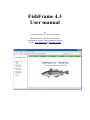
1
FishFrame 4.3
User manual
By
T. Jansen, H. Degel & Users of FishFrame
Danish Institute for Fisheries Research
Charlottenlund castle, Charlottenlund, Denmark
E-mail: [email protected], & [email protected]
26 January 2007
Table of content
Introduction....................................................................................................................4
The system .....................................................................................................................4
Data ............................................................................................................................4
Coverage ................................................................................................................5
Stratification...........................................................................................................5
Data policy .............................................................................................................5
Software and hardware requirements.........................................................................6
Project notes...............................................................................................................6
User interface .............................................................................................................6
Security ..........................................................................................................................7
Logon .........................................................................................................................7
Levels of access (roles)..............................................................................................7
Functionality ..................................................................................................................8
Data browser ..............................................................................................................8
Reports .......................................................................................................................9
Analysis....................................................................................................................12
Data action – Data mainenance................................................................................15
Commercial samplings (disaggregated)...............................................................16
Landing statistics .................................................................................................29
Effort statistics .....................................................................................................29
Acoustic survey data (detailed, stage 1) ..............................................................29
Acoustic survey data (compiled, stage 3) ............................................................29
Data action - Data integration ..................................................................................29
Commercial fisheries ...........................................................................................30
Acoustic surveys ..................................................................................................30
Data action – Tools ..................................................................................................30
Info & Help ..............................................................................................................32
Tutorials ...............................................................................................................32
Documentation.....................................................................................................33
IT-Support............................................................................................................34
Misc..........................................................................................................................34
Refresh .................................................................................................................34
Security ................................................................................................................34
Contact .................................................................................................................35
Links ....................................................................................................................35
Generic components.................................................................................................36
Pivot tables...........................................................................................................36
Pivot charts...........................................................................................................37
Pivot maps............................................................................................................38
SVG diagrams......................................................................................................41
Simple tables........................................................................................................41
Future versions, planning and bug handling ................................................................42
Errors and crashes ....................................................................................................42
Version planning......................................................................................................43
System testing ..........................................................................................................43
Technical stuff .........................................................................................................43
Recommended timing of workflow for assessment WG’s ..........................................43
2
26 January 2007
Documentation of aggregation and calculation procedures.........................................43
CANUM, Mean weight, Age-length & Standardized length distribution ...............43
Processes creating Standardized length distribution (SLD).................................46
Processes creating the Age-Length Key (ALK) ..................................................46
Processes creating the Standardized CANUM (stCANUM) ...............................47
Processes creating the mean weight.....................................................................48
Discard fraction........................................................................................................48
Weight..................................................................................................................48
CPUE .......................................................................................................................49
Weight..................................................................................................................49
Acoustic survey data ................................................................................................50
Calculation of global abundance estimates, mean weight and mean length........50
Interpolation of global abundance estimates, mean weight and mean length......50
References....................................................................................................................52
Appendices...................................................................................................................53
Appendix I ...............................................................................................................53
Appendix II ..............................................................................................................54
Overview..................................................................................................................54
Terminology.............................................................................................................54
Check sets ................................................................................................................54
Check-set creation................................................................................................54
Check creation .....................................................................................................55
Check-set execution .............................................................................................57
Importing check-sets, data-set definitions and checks.........................................58
Security (Who can do what) ....................................................................................59
3
26 January 2007
Introduction
This document describes how to use all the features in FishFrame. It is also the place
where users can exchange descriptions of “best practice”. All contributions are
welcome and can be mailed to the administrator.
This document covers all standard FishFrame “clones”, i.e. “FishFrame Baltic Sea”,
“FishFrame North Sea” and “FishFrame FantaSea” even though the Baltic clone is
chosen for illustrations etc. A separate user manual can be found for the
FishFrameAcoustics “clones”.
Other documentation can be found on the documentation page under “Info & Help” or
it can be requested from the FishFrame staff.
The versioning of this document follows the date stamp in the upper right corner on
all pages except the front page. The latest version is always available from the
FishFrameAcoustics website.
The system
FishFrame is an existing web based datawarehouse application that can be accessed
on www.FishFrame.org.
FishFrame is the link between stored nationally raw data and the aggregated data used
in the assessment process.
The main workflow in FishFrame brings data through data checking, raising,
extrapolation and export to assessment tools. The data status is tracked along this path
and relevant information is available to the user in interactive reports and analysis.
The data confidentiality and access to data manipulation tools is handled under a tight
role-based security system.
FishFrame is an open source project. The free licensing policy is described in the
FishFrame License document found on the documentation page. A full set of source
code for the latest version can be obtained by contacting the FishFrame team.
Data
FishFrame contains all fisheries assessment relevant data except data for establishing
commercial tunings fleets. The assessment relevant data include:
• Biological information of the landings obtained by sampling from market.
• Biological information of the catch (discard as well as retained part compiled
separately) obtained by observers participating in regular fishery.
• Biological information of the catch (discard as well as retained part compiled
separately) collected by the fishermen themselves.
• Official landings statistics by two different aggregation levels.
• Effort statistics by two different aggregation levels.
• Data from Acoustic surveys (integrated scrutinized NASCs, biological
information from the catch).
• Scientific demersal trawl survey data on exchange format.
4
26 January 2007
All biological information is basically on disaggregated form (haul/set for sea and
harbour sampling and single sample level for marked samples).
Results from scientific demersal trawl surveys (not acoustic surveys) are copies of the
data uploaded to the ICES database, DATRAS.
The variables included in FishFrame should satisfy all data needs for most assessment
models including fishery based assessment models. For a complete list of variables
included please consult the exchange format specifications found under “Info &
Help” -> “Documentation”.
Coverage
It is the aimed that all countries having interests in the Baltic Sea and/or the North
(EC member states and non-member states, ICES member states and non-member
states) will upload data to FishFrame. The more complete the data are the better use
can be made of FishFrame. For an updated overview of the data in the database,
please use the reporting facilities available in FishFrame.
Stratification
The national data collection schemes are to a wide extent stratified on common
definitions. These definitions include strata based on
• Time periods (month or quarter)
• Areas (division, sub-division, statistical rectangle)
• Fishing Activity Category
The “Fishing Activities” are based on the definitions finalized during the Nantes
Work Shop in June 2006 (anon, 2006).
The activity stratification is hieratic constructed. The Fishing activities resemble the
so-called Regional Level (level 6) which is based on gear type, mesh size, and
regulation constrains. For a detailed description of the Fishing Activity system, see
(anon, 2006) and for a list of criteria defining the different Fishing activities, please
see “Reports”→ “Stratifications” → “Fisheries” in the FishFrame menu.
Data policy
The national data in FishFrame is owned by the national institutes. Each national
institute updates their own data when changes are made in the data source (the
national database containing the raw data). FishFrame is a datawarehouse that only
contain copies / derived outputs from the national databases.
Access to viewing and analyzing other countries data in FishFrame does not entail
permission to download, copy or publish dis-aggregated not-own-country data outside
FishFrame. Such permissions can only be granted by each national institute. The
request can be put forward by using the form in appendix I, giving detailed
descriptions of the data needs and the use of data. Data can normally only be used by
the scientific community for scientific purposes. Only national "editors" and
"administrators" can do such download.
While most of the data are visible for all users in FishFrame, some are confidential.
The confidential data are masked by “***” for users from other countries. Data
considered confidential in FishFrame are:
• Longitude and latitude of stations of commercial samples (sea sampling).
5
26 January 2007
•
•
Length frequency data from commercial data. The exact number at length and
catch weight is masked, rest is visible.
Unallocated and area-misreported landing statistics.
Software and hardware requirements
The client side requirements are listed below, while the server side setup is
documented in the developer’s manual. See also the “FishFrame Tech note” on the
documentation page.
•
•
•
•
•
•
Web browser (tested on MS Internet explorer 7.0., Mozilla Firefox 2.0*, and
Opera*)
Pop-up windows enabled.
MS Office XP Web Components (part of full office XP installation). This is to
be able to use the pivot tables and charts.
Adobe SVG-viewer (free software). This used in the outlier analysis.
Adobe reader (free software) or similar to read documentation in PDF-format.
Internet access 30 Kb is sufficient (except for tutorials), more is nice.
* Pivot tables and outlier analysis will only work in Firefox from version 4.3 in December 2006)
Details on installing and setting up software can be found online under “Info & Help”
/ “IT-Support”.
Project notes
It is very important for the FishFrame team that all effort is made as a bottom-up
process. E.g. close cooperation between developers, architects and end users. It is in
our view the most effective method to add true value to end users.
The project has so far been managed by DIFRES and all software has been written by
software developers in DIFRES. We would like to widen the management/design
group and formalize it. Furthermore we welcome any non-DIFRES software
developers. The existing software architecture (modules) provides the basis for a
distributed development.
Hosting of the FishFrame servers has so far been done by DIFRES. This could
continue as long as the participating labs are satisfied. Hosting could also be handled
by any other lab.
User interface
The screen is split into three areas (Figure 1):
1. The left frame contains the logon page from start and a data tree after the user
has logged on.
2. The green menu in the upper part of the right frame. The menu is expanded
when the mouse is moved over a part of the menu. Item are selected by single
clicking. A black triangle indicates that the menu can be expanded further.
3. The main screen in the rest of the right frame.
6
26 January 2007
All the functionality is covered menu-point by menu-point in the designated chapter
below.
Figure 1. FishFrame web application before logging on.
Security
FishFrame contains confidential data; therefore only valid users with a secure set of
logon credentials can access the data.
Information about changing user details like email and password can be found in the
designated chapter under “Functionality” below.
Logon
Log on using the username (=email) and password given by the administrator.
It is possible to get a mail with the password, if it has been lost. Enter the email in the
“user name” field and press the “mail password” button found in the lower part of the
left frame (Figure 1).
If a wrong password is entered two times, then a warning is issued and on the third
attempt; the account will be locked. Only the administrator can unlock the account.
Every time the log on attempt is successfully, the counter is reset, so there is no risk
for account lockout by mistyping the password now and then.
Levels of access (roles)
The level of access (role) is one of the following four:
1. Reader
2. Editor
3. (Stock coordinator)
4. Administrator
7
26 January 2007
“Stock coordinator” will be added to the system in the next release.
The functionality available to each role is listed in Table 1.
+
+
+
+
+1
+1
+1
-
+
+
-
(Stock editor)
Administrator
+
+
+
+
+
+
+2
+2
+2
+2
+2
+2
+
+
+
Table 1. Available actions by role. +1 = only from own country, +2 = from all countries
Functionality
The functionality will be presented here in the same order as it is found in the menu.
Notice that the content of the menu is role-dependant, so the choice of functionality
will always match what your security level permits you to access.
The menu (Figure 2) contains five top items that can be expanded.
Figure 2. The main menu
The submenus under each item are explained below:
Data browser
The type of data to be explored using the data
tree in the left pane can be selected.
The tree in the left frame in the tree based data
browser (Figure 4) are used to navigate through
the data, while the actual data are presented in a
Figure 3. Selection of data browser
table in the right frame.
A node in the tree is expanded by clicking the
“+” and collapsed by clicking the “-”. When clicking on the label (text), the node is
toggled (expanded or collapsed) and the data represented by the node is shown in the
table. The table is a “simple table”. The functionality of a simple table is described in
the designated chapter below.
8
Add & edit users
Release stock for
assessment
Edit own user account
Apply-estimate missing
strata
Validate and release data
Upload / download data
View data in
reports and analysis
View data through tree
+
+
Role
Read documentation
Reader
Editor
Action
26 January 2007
Figure 4. The tree based data browser
Reports
All output related to overview of the content
of the database and reports that do not require
much analytical processing is found under
“Reports”. The reports are described in Table
2. Most of the reports are pivot tables, pivot
charts, pivot maps or simple tables. The
functionality in these reports is described in
Figure 5. Selection of report
9
26 January 2007
the designated chapter below.
Report
Commercial
samplings
Landing statistics
Effort statistics
Type
Samples
Pivot table,
-map
and -chart
Description
The number of stations.
Remember to select a fisheries set,
otherwise the number will be
multiplied by the number of fishery
sets.
Length
Pivot table, The number of length measured
measures
-map
individuals.
and -chart
Remember to select a fisheries set,
otherwise the number will be
multiplied by the number of fishery
sets.
Otolith
Pivot table, The number of age determined
measures
-map
individuals in the representative
and -chart
subsamples.
Remember to select a fisheries set,
otherwise the number will be
multiplied by the number of fishery
sets.
Length freq.
Dialog
List of length groups without
data without
->
corresponding individual age
corresponding Simple table distribution.
age
Country, year and quarter are
selected before the report is created.
Length freq.
Dialog
List of length groups without
data without
->
corresponding individual weight.
corresponding Simple table Country, year and quarter are
weight
selected before the report is created.
Data status
Pivot table, The average of the last successfully
and -map
completed step.
Raising
Simple table The settings to be used when
options
compiling data. These settings will
be country-, stock- and year specific.
Notice: these settings are currently
under evaluation and are therefore
not implemented in the compilation
procedures.
Landing
Pivot table, The sum of official landing statistics
statistics
-map
(not including the information about
and -chart
misreporting). These are the landings
uploaded as “L1” and “L2”-format.
Data status
Pivot table, The average of the last successfully
and -map
completed step.
Effort
Pivot table, The sum of “number of trips”.
statistics
-map
Sum of “Number of sets / hauls”, “Fishing
time / soaking time” and “kW-days “ can
and -chart
be pulled into the table instead of
10
26 January 2007
Acoustic survey
Trawl survey
Data status
Pivot table,
and -map
Detailed data
(stage 3) ->
Abundance
Detailed data
(stage 3) ->
Stock detail
(fractions)
Samples
Pivot table,
-map
and –chart
Pivot table,
-map
and –chart
The Abundance and milage
Pivot table,
-map
and -chart
Pivot table,
-map
and -chart
Pivot table,
-map
and -chart
Various
The number of stations.
Length
measures
Otolith
measures
ICES tools &
info
Strata definitions
“number of trips”. These are the
efforts uploaded as “E1” and “E2”format.
The average of the last successfully
completed step.
Countries
Acoustic
surveys
Ships
Fisheries
Gear
Survey gear
Area -> Stat
rect. To area
Area -> Area
to area
Area ->
Adjacent
areas
Area ->
The fractions, mean weight and
mean length at age-maturity-stock.
The number of length measured
individuals in the representative
subsamples.
The number of age determined
individuals.
Various web-based reporting and
mapping services available from
ICES and sister institutes. All
presents the same trawl survey data
found in FishFrame and DATRAS.
Simple table List of country codes
Simple table List of acoustic survey codes
Simple table List of survey ship codes
Simple table List and definition of the fishery
codes (Fishing Activity Categories).
Simple table List of Gear codes
Simple table List of gear codes for gear used by
survey ships.
Simple table The relations between statistical
rectangles and areas. Some statistical
rectangles overlap two areas, but in
the calculations they are being
treated as belonging to a specific
area.
Simple table The relational hierarchical structure
of the areas.
Simple table The definitions of which areas that is
“adjacent” to which.
Simple table List of codes that can be used for
11
26 January 2007
Biological
subareas
Area -> SubStatisticalRectangle
Species
Acoustic
species
(/Species
groups)
Stocks
Sub-stocks
Maturity
scale
Biological areas in acoustic data.
Simple table List of sub-statistical-rectangle
(quarters of a rectangle).
Simple table List of species codes
Simple table List of “acoustic species / groups”
codes to be used in acoustic data.
Simple table Definitions of stocks.
and pivot
table
and -map.
Simple table Sub-stock codes and their definition
Simple table Maturity scale codes
Table 2. Descriptions of reports.
Analysis
All output that require analytical processing
is found under “Analysis”, this includes
input to stock assessment models made
during data action step 10 “WG stock
release”. These reports are described in
Table 3. Most of the reports are pivot tables,
pivot charts, pivot maps or simple tables.
The functionality in these reports is
Figure 6. Selection of analysis
12
26 January 2007
described in the designated chapter below.
Report
Commercial
samplings
Type
Description
Age-LengthWeight
outlier
analysis
Age-Length
relations
Special
See description in designated chapter
below.
Pivot table,
and -chart
Standard
length distr.
Pivot table
and -chart
Age-length key. Fractions for each
age for a given length. Row totals
are always 1. Includes age
regressions per default, but this can
be altered and explored by
modifying the regression-dimension.
For aggregation and regression
details; see designated chapter
below.
Standard length distribution.
The normalized length distribution.
For aggregation details; see
designated chapter below.
Species distribution in sea/harboursampled catches. Individual catches
are standardized (raised) to 1 tonnes
of total catch. Samples with validity
code 4 is excluded from this report.
Multiple samples within same
stratum are aggregated as an average
1 tonnes catch. Each sample is given
equeal weighting in the average.
Zero catch for a given species in a
given stratum affects the average if:
1) The species is represented in
a stock living in the area
(ICES sub-area).
2) There is sampled catch of
any species within the same
stratum.
“Weight”can be pulled into the table
instead or together with the
“number”. This opens up for the
possibility to make calculated
measures based on both measures.
DO NOT remove “Species” from the
axes.
Species distribution in sea/harboursampled catches. Individual catches
are standardized (raised) to 1 tonnes
of total catch. Samples with validity
code 4 is included from this report.
Species
Pivot table,
distribution in -map
sampled
and -chart
catches -> In
numbers
Pivot table,
Species
distribution in -map
sampled
and -chart
catches -> In
weight
13
26 January 2007
CPUE weight
per hour
Pivot table,
-map
and -chart
Discard
fraction. By
weight
Pivot table,
-map
and -chart
Mean weight
Pivot table,
-map
and -chart
Standardized
CANUM
(Admin only)
Pivot table,
-map
and -chart
14
Multiple samples within same
stratum are aggregated as an average
1 tonnes catch. Each sample is given
equeal weighting in the average.
Zero catch for a given species in a
given stratum affects the average if:
3) The species is represented in
a stock living in the area
(ICES sub-area).
There is sampled catch of any
species within the same stratum.
DO NOT remove “Species” from the
axes.
Catch Per Unit Effort.
Catch weight per hour of fishing
effort. Zero-catches are included, it
is therefore crucial to select fishery
and dataset with care (the dataset
could include stations where only
cod was reported, thereby indicating
a false zero-catch of other species).
However catches outside the stocks
distribution area are excluded.
Marked sampling data are excluded
as well.
The fraction of the catch that was
discarded. Calculated as a simple
mean discard weight fraction of the
catch weight. Zero-landings and
zero-discards are included, it is
therefore crucial to select fishery and
dataset with care (the dataset could
include stations where only cod was
reported, thereby indicating a false
zero-catch of other species).
Mean weight in grams by age-group.
Includes weight regressions per
default. For aggregation and
regression details; see designated
chapter below.
The mean weight can also be
calculated by lengthclass if this field
is dragged onto one of the axes. If
length class and age are on the axes,
then the report displays the basic
mean weight based on CA-records,
not weighted by catches.
Standardized catch in numbers by
age group. Standardized so that it is
in 1000 specimens per 1000 tonnes
26 January 2007
Data integration
landings.
This table can be used to get the
discard by landings. Remember to
select a fisheries set, otherwise the
number will be the sum of the values
for all fishery sets. For aggregation
and regression details; see
designated chapter below.
Catch in numbers by age group
(landings as well as discards. raised
data as well as apply-estimated
data). Remember to select a fisheries
set. For aggregation and regression
details; see designated chapter
below.
Number of specimens in the total
stock estimate.
All zero-values (measured and
unmeasured are not shown in this
report or they appear as empty cells).
Weight (tonnes) of specimens in the
total stock estimate.
All zero-values (measured and
unmeasured are not shown in this
report or they appear as empty cells).
A zero in this report indicated a
weight rounded off to 0 tonnes, i.e.
less than 500 Kg but more that 0 Kg.
CANUM
Pivot table,
-map
and -chart
Acoustic
surveys ->
Total Stock
Estimate
(abundance)
Acoustic
surveys ->
Total Stock
Estimate
(weight)
Pivot table,
-map
and -chart
Acoustic
surveys ->
Total Stock
Estimate
(mean
weight)
Acoustic
surveys ->
Total Stock
Estimate
(mean length)
Pivot table,
-map
and -chart
In Grams
Mean weight of specimens in the
total stock estimate.
Pivot table,
-map
and -chart
In mm.
Mean length of specimens in the
total stock estimate.
Pivot table,
-map
and -chart
Table 3. Descriptions of analysis.
Data action – Data mainenance
All the work steps in the data flow from uploading raw data, data screening and data
handling is found under “Data action” -> ”Data maintenance”.
Figure 7. Selection of data actions
15
26 January 2007
Commercial samplings (disaggregated)
1. Upload & first check
Consult the exchange format specification for information about the content of the
data file. The exchange format specification can be found on the documentation page
under “Info & Help”.
The overwrite-rules are described below.
The upload-file is selected in the dialog window that pops up after pressing the
“browse”-button on the upload page (Figure 8).
Figure 8. The upload page. Lower part of the page presents a list of recent changes in the exchange
format.
The system then runs through the following steps:
1. Uploads the file to the server.
2. Key value consistency check (not for XML-upload).
Checks if parent and child records are matching (e.g. that HH country field is
the same as all the HL’s country fields).
3. Conversion to XML (not for XML-upload)
4. Duplicate record check.
This ensures that lines that are required to be unique with respect to the key
parameters (e.g. HH and HL records in CS-files) do not exist as duplicates.
This step is skipped and then performed during saving for large LS and AA
files.
5. Data check.
a. All the range- and enumeration-checks specified in the exchange
document. Enumeration checks are checks where valid values are
given in a list.
16
26 January 2007
b. Checks if mandatory fields has a value.
c. Check on the XML structure.
If all steps are passed without errors like in Figure 9, then the data can be inserted into
the system. Click on the link “Yes” to insert the data otherwise; just navigate away
from the page using the menu. A successful saving will be reported in the addition of
two lines stating:
- FishFrame successfully updated.
-> The upload of you data completed successfully.
When the data are inserted, they might overwrite old data for the same stratum. The
overwrite-rules are:
• Commercial sampling: By Year, Country, Journey.
• Landing statistics: By Year, Quarter, Country and Species.
• Effort statistics: By Year, Quarter, Country and Species.
• Acoustic data (aggregated / stage 3): By Survey, Year, Ship and species.
• Acoustic data (dis-aggregated / stage 1):
o Fishing: By Survey, Year and Ship.
o Acoustics: By Survey, Year and Ship.
Figure 9. All checks have been passed without errors.
If errors are detected in the file in any of the checks, then the process will stop
immediately and the feedback line will state the number of errors found, which check
that found them and provide a link to a detailed error report (e.g. “- Data check
complete: 78 Errors were found. View error report.”). The error report is specific for
each check. An example of a key value consistency error report can be seen in Figure
17
26 January 2007
10, a duplicate record error report in Figure 11 and a data check error report in Figure
13. The error reports are explained here:
Key value consistency error report (Figure 10).
The given example is from a data file with a HH record with two erroneously HL
records. The country field in the HH record is set to “TST”, while the first HL has
“XXX” and the second has an empty field “”. Both errors are visible on the error
report. The error report states in the header row that the first error is from a “record
type” HL. It also gives the location in the file; “ASCII line (parent)” is 1 (so this is the
HH record in line 1) and the “ASCII line (child)” is 2 (so this is the HL record in line
2). Below the header row there is a table with all the parameters that should be alike
in the HH and HL. The error in the country field in HL is easily spotted in the table.
Figure 10. The key value consistency error report
Duplicate record error report (Figure 11).
The given example is from a data file where the two first lines are L1 (aggregated
landings) that are identical in all the key parameters. As it can be seen in the report by
looking at the two columns named “ASCII line number” the errors were found by
comparing line 1 and 2. The identical natural key can be seen in a special sub-report
(Figure 12) by clicking on the “Natural key” link in the rightmost column. This is
18
26 January 2007
important information for finding the error if the upload format used is XML but also
useful for CSV-file uploading.
Figure 11. The duplicate record error report.
Figure 12. The natural key report from the duplicate record error report.
Data check error report (Figure 13).
The given example is from a file with 24 errors of various kinds. They are all of the
types: out of range, invalid value or missing mandatory field. See the first line in the
report; here it is stated (reading columns from left to right) that the error is in the field
“SpeciesCode”, the record type “HL”, record number “1” (this is the first HL record),
Journey number “806”, station number “1” and the erroneous value was “XXX”. The
comment describes that it was an illegal value for that field and gives a link to the list
of valid values (Figure 14). The natural key can be seen in a special sub-report (Figure
15) by clicking on the “Natural key” link in the rightmost column. This is important
information for finding the error if the upload format used is XML, but also useful for
CSV-file uploading.
19
26 January 2007
Figure 13. The data check error report
Figure 14. Acceptable enumeration values report from the data check error report.
20
26 January 2007
Figure 15. Natural key report from the data check error report.
2. Second check
This is a mandatory step.
The second check is the check where the last requirements described in the exchange
document is performed. These requirements are dependencies between fields, e.g. the
field “VesselLength” is mandatory, but Optional if gear is "fixed gear".
On the first page (Figure 16) the data set is selected. A “Check” button appears after
year and country had been selected. Quarter and area are optional. Care should be
taken when selecting data set, because the checker will stamp the data with data status
“2” as “last step” even if some of the data has already been released and thereby has
the data status “6”. This especially applies to countries where different labs upload
data from different areas or if data are uploaded quarter by quarter.
When clicking on “Check” the data checking routine is executed and the result is
displayed as seen on Figure 17 (passed) or Figure 18 (not passed). If the data does not
pass the checks then the input data should be corrected in the national database, a new
upload file should be generated and uploaded. Data status is kept on “1” if the data
does not pass the check.
Figure 16. Select data set for second check.
21
26 January 2007
Figure 17. Result of the second data check. The data did not pass all the checks. Exact information is
given so the input data can be corrected.
3. Approve (Outlier analysis)
This is an optional step.
After selecting the country and year in the first dialog form, then a table like Figure
18 appears. The table gives overview over which strata that already have been
approved. Green links mean “approved” while red indicates “not approved”. There
are two links for each combination of Species, SpawningType, Area and Quarter. The
first link is for age-length relations and the second is for length-weight relation. Click
on a link to get the corresponding outlier analysis (OA).
22
26 January 2007
Figure 18. Outlier analysis overview table for Denmark 2003.
The web browser needs a plug-in installed for viewing the OA diagrams. The plug-in is
free and details about downloading and installing it can be found under “Info &
Help”/”IT-Support”/”Help on charts”.
The diagrams have some functionality like zooming. See the description of SVG
diagrams in the chapter “Generic components” below.
The data in the OA diagrams (Figure 19) are indicated by green points, except for the
outliers which are red and disabled data which are grey. The yellow line is the
regression. Any point in the chart can be explored by single-clicking it. If the points are
in a cluster, then zooming in will make it easier to select the right one. When selecting a
point, all its information pops up in a table in a new window (Figure 21). The data point
can then be disabled or enabled and a proper reason can be entered for documentation
purposes. If a data point is disabled, it is not used in any further analysis.
If the data are satisfactory for further analysis, then the button “Click here to approve
this stratum” is pressed, and the user is redirected to the overview table (Figure 18).
Outlier criteria.
Based on the data submitted to the database an outlier analysis is made to identify
data points that could be erroneous. Regressions are made on length-weight and agelength relationship. The data are stratified by year, country, species, area and quarter.
The length-weight relationship is described by:
Weight = a * length b
The constants a and b are estimated by regression on the linear zed equation and the
theoretical length-weight curve are drawn. Outliers are identified if they exceed:
2 * standard error
of the observed values.
The age-length relationship is described by the von Bertalanfy’s growth equation:
L(t) = l∞ * e-k(t-t0)
23
26 January 2007
The constants l∞ and -k should be estimated by a non-linear regression but is in the
current version estimated by a Beverton-Holt plot (which gives a rather poor fit with
few data) and outliers are identified if they exceed:
2 * standard error
of the observed values.
Figure 19. Length-weight outlier analysis for Denmark, 2003, Q1, Cod and area 21.
The length-weight OA (Figure 19) consists of up to 8 diagrams; one for discard and one
for each size sorting of the landings. No diagram is presented if less that three data
records are present (e.g. for landings and size sorting 1 in Figure 19). An example of
outliers can be seen in Figure 20, the three outliers are easily noticed due to their red
colour. Disabling one (the 460 g 57 cm cod on Figure 21) makes the OA to be rerun
without this point (Figure 22). Since this decreases the standard distribution, it makes
more points turn into outliers. The disabled point is greyed out.
24
26 January 2007
Figure 20. Length-Weight outlier analysis diagram with three outliers.
Figure 21. Pop-up window with a single data point (CA record) from OA and the functionality to
manage it.
25
26 January 2007
Figure 22. OA diagram from Figure 20 after disabling a data point.
The age-length OA (Figure 23) consists of a single diagram. No diagram is presented if
less that three data records are present. The regression procedure in the current version
is rather poor and will be changed as soon as possible. However the plot is still of great
value to spot data points that sticks out.
26
26 January 2007
Figure 23. Age-Length outlier analysis diagram with two outliers.
If larger errors than just a single strange data point are detected, the workflow is to go
back to the raw data in the national database, correct the error, make a new upload file
and start with step 1 again.
When all links has been changed to green by checking and approving all data, the user
can move on to step 4. Since step 3 is an optional step, it can be skipped if the time plan
makes it impossible.
4. Advanced check
This is an optional step.
The user guide for this module is extensive and has therefore been placed separately
in Appendix II.
A set of default checks exists in the system and will typically be the starting point for
the user. Users can then add, delete and modify checks in their own copy of the set,
run it and save it for later use. A filter can be added, so the user runs the checks on a
subset of the data. A user can have several sets of checks.
The types of checks are:
• Simple value comparisons.
• Range (max-min and enumeration) checks depending on other fields
e.g. “Age is between 0 and 25 if species is cod”
• Formula based dependency checks like: Weight = k*(Length) 3, where
k is dependent on the species (and maybe Quarter and area too).
The two prior checks are actually just simple checks of this type.
5. Confirm raising settings
This is an optional step.
27
26 January 2007
Check the settings for the country, year, stovk and catch category that are worked on.
Move on to step 6 if they are correct, otherwise get the administrator to change them
(an editor page is under development).
Figure 24. Country-year-stock-CatchCategory specific settings for the aggregation procedures.
6. Release
This is a mandatory step.
After quality assuring the data, they are released to further international work. The
data status is changed indicating that these data are now ready to be used in
international work.
CS data: The data is now included in the analysis: “Standardized length distribution”,
“Age-length key”, “Mean weight” and “Standardized CANUM”.
Figure 25. Test data from 2001 was released successfully.
28
26 January 2007
Landing statistics
1. Upload & first check
Same as for “Commercial samplings (disaggregated) step 1”, please refer to that
chapter above
2. Advanced check
Same as for “Commercial samplings (disaggregated) step 2”, please refer to that
chapter above
6. Release
Same as for “Commercial samplings (disaggregated) step 6”, please refer to that
chapter above
Effort statistics
1. Upload & first check
Same as for “Commercial samplings (disaggregated) step 1”, please refer to that
chapter above
6. Release
Same as for “Commercial samplings (disaggregated) step 6”, please refer to that
chapter above
Acoustic survey data (detailed, stage 1)
1. Upload & first check
Same as for “Commercial samplings (disaggregated) step 1”, please refer to that
chapter above
6. Release
Same as for “Commercial samplings (disaggregated) step 6”, please refer to that
chapter above
Acoustic survey data (compiled, stage 3)
1. Upload & first check
Same as for “Commercial samplings (disaggregated) step 1”, please refer to that
chapter above
6. Release
Same as for “Commercial samplings (disaggregated) step 6”, please refer to that
chapter above
Data action - Data integration
All the work steps in the data flow concerning rasing, aggregation and estimation of
data is found under “Data Action” -> “Data integration”.
29
26 January 2007
Commercial fisheries
This is a mandatory step.
<To be written>
Acoustic surveys
National raising -> Calculate national estimates (stage 2)
This step is under development
International compilation -> Calculate global estimates
First select the year and Species. The system then calculates number, weight, mean
weight and mean length at age, maturity, stock, stat.rect, etc.
Figure 26. Global estimates for Herring in the 2006 HERAS survey was calculated successfully.
Note that measures zeros are not stored! All relevant rectangles are presumed to be
covered in the survey - if holes exist then they will be interpolated later in the
interpolation step.
International compilation -> Interpolate missing rectangles
Select the year, species and rectangle that should be estimated by interpolating the
values from available data from the neighbouring 8 rectangles.
Data action – Tools
All the available tools and test data that can be used to assist the work done under
“Data maintenance” and “Data integration” can be found under “Data Action” ->
“Tools”.
Test data
This section contains all the data used in the structured acceptance test. The tests and
usage of the test data is described in the test document that can be found on the
documentation page.
Excel exchange format
This is the excel sheet previously used to submit data to the coordinator (John
Simmonds). The sheet has existed in several versions through the years. The version
that can be downloaded here is the version from 27 September 2005.
Notice that it is important to keep the formatting, since this reflects the formatting in
the upload format (e.g. abundance as numeric with 4 decimal places) and the
exchange format converter reads the cell contents as it appears in the formatted form.
Do not add rows, columns or calculated cells (or do it in a separate copy that will not
be fed into the converter program).
Exchange format converter
30
26 January 2007
A program that can convert data in excel sheet (version 27 September 2005) to data in
XML upload format can be downloaded and installed here (Figure 27). It is important
not to change anything else than the values in the cells containing abundance, milage,
fraction, mean weight and mean length. The format of these cells should remain
untouched as numbers with the preset decimal places. If the format is changes it will
affect the precision and rounding in the conversion. To avoid this it is recommended
that all data are copied into the sheets using “Edit”->“Insert special…”->”Values”
from the excel menu.
Notice that XML is the primary exchange format – not the excel sheet. The
description of the XML exchange format is in a separate document that can be
downloaded from the documentation page under “Info & Help”. The converter
program has been developed mainly to convert old data files so they can be uploaded.
The program does not handle all sorts of incorrect excel-sheets in a very user-friendly
way – it will crash if the file is wrong. If it should crash then make sure that it is the
right version of the excel sheet and that there has not been any changes to the
placements of the cells. Try downloading the sheet and only copy the data into the
sheet. If this should not help, then mail the sheet to the administrator, who will be able
to help. It is recommended that programs to extract data from databases and format
directly into XML are made nationally.
This section describes how to use the converter program.
Figure 27. Download page for the exchange format converter application.
The program will, after installation, be accessible from “program files” like other
programs on the PC (Figure 28).
Figure 28. Start the converter program under FishFrame->FishFrameAcoustics in the program files.
The application only consists of one form (see Figure 29). On this form the year,
country, ship, Species and stock is selected. The path and name of the excel file to
convert is either entered manually or selected by clicking “browse”.
The button “Clear form” removes all entries in the textboxes.
The button “Create XML” starts the conversion process indicated by the progress bar
that shows up below the button. When the process ends the result is written above the
progress bar as seen on Figure 30. The two newly created XML files is places in the
same folder as the excel sheet. Their names are concatenations of: Country + ship
code + year + file type (e.g. “Denmark DAN2 2005 AB.xml”).
The XML files are then ready for upload. Manual editing in the files can be done with
a normal text editor like “notepad” or a special XML editor like “XML-spy”.
31
26 January 2007
Figure 29. The user interface in the conversion application.
Figure 30. Conversion ended successfully.
Info & Help
All documentation, tutorials and help on how to use
FishFrame, interpret data or format upload files is found
under “Info & Help” (Figure 31).
Tutorials
The tutorials are small film clips that can be downloaded
(Figure 32). They come wrapped in a player, so they do
Figure 31. Selection of info & help
not require any special software to be viewed. Click on
the link to open or download the tutorials.
Notice that they are quite large for a thin internet connection (up to 7 MB).
32
26 January 2007
Figure 32. The tutorials page, where film clips can be downloaded.
Documentation
The documentation is in pdf format, which can be viewed in the free adobe reader.
Click in the link to open or download the document.
Figure 33 The documentation page.
33
26 January 2007
IT-Support
In this section there are three pages with guidelines for setting up the computer to use
different features in FishFrame.
•
•
Help on reports
This is the pivot based reports and analysis
Help on charts
This is the charts used in the outlier analysis
Misc.
All security features and contact
information is found under “Misc.” (Figure
34).
Refresh
This navigates all parts of FishFrame to the
beginning, as if the user had just logged
on. Use this if the menu item that is
needed is “hiding” under an element on
the screen (the menu goes underneath
elements such as drop-down boxed,
buttons and pivot tables).
Figure 34. Selection of miscellaneous
functionality
Security
Update user details
The name and email address can be changed on the form depicted in Figure 35.
Administrators can also change the country and role.
Figure 35. Update user details form
34
26 January 2007
Change password
It is required to retype the password; this is to avoid problems for the user in case of
involuntary mistyping of passwords (the password is masked as **********, so a
visual quality check is not possible).
There is a password policy to avoid hacking. The policy does now allow the password
to be equal to any part of the name or email. The password should also be minimum 6
characters long and preferably contain letters, numbers and special characters.
New user
The administrator can create new users using the designated form (Figure 36).
Figure 36. The form where new users are crated.
Activity report
The activity report is a pivot table that can be used to analyse the usage of FishFrame.
Contact
Email links to:
•
•
•
The FishFrame staff
The editors uploading data from countries
All users
Links
A list of links to related online databases, international organisations and the
institutions using FishFrame.
35
26 January 2007
Generic components
The generic components are blocks of the user interface, that are used several places
in the application. The functionality of the components are independent of the specific
implementation and are therefore described separate from those chapters.
Some of the components require some kind of installation. The details of this can be
found under “Help & Info”/”IT-Support”.
Pivot tables
A PivotTable (Figure 37) is an interactive table that can be used to analyze data
dynamically. Some of the features are:
•
•
•
•
•
•
•
•
•
Filtering data
Sorting data
Grouping data
Summing up, calculating from
Formatting
Copy data to other programs
Dump data to excel and continue dynamic work there
Moving, adding and removing fields
Drilling down, drilling up, slicing, and dicing data.
Most of theses features are accessible when right clicking an item (e.g. a field for
field-working with properties or on the green header bar for table-properties.
The functionality is described in the “MS Office Pivot table component help” that is
being reached by pressing the “?”-icon on the upper right corner of the pivot table.
The help document is well structured and gives quick access to specific info through a
navigation tree or a search.
36
26 January 2007
Figure 37. A pivot table displaying landing statistics.
More information about pivot tables can be found at:
http://msdn.microsoft.com/office/understanding/owc/
Pivot charts
A pivot chart (Figure 38) is a chart that is driven dynamically by the data in an
accompanying pivot table. It shares all the features of a pivot table.
The functionality is described in the “MS Office chart component help” that is being
reached by pressing the “?”-icon on the upper right corner of the chart. The help
document is well structured and gives quick access to specific info through a
navigation tree or a search.
37
26 January 2007
Figure 38. A pivot chart displaying number of stations by year and country.
More information about pivot charts can be found at:
http://msdn.microsoft.com/office/understanding/owc/
Pivot maps
A pivot map (Figure 39) is a map based on the content of a pivot table.
To create a map:
1. Make sure that there are no fields on the column-axis
2. Make sure that there is only a geographical field (area or statistical rectangle)
on the row-axis.
3. Press the “Create map” button.
The pivot map features are:
• Zoom in
1.
2.
3.
4.
Select the “ ”-button in the row of buttons (upper right area).
Move the cursor over the map, the cursor is now appears as a “+”.
Click on the corner of the area that should be zoomed to.
Hold the mouse button down while dragging to the opposite corner of the
area; the area is now marked by a black box.
38
26 January 2007
•
5. Release the mouse button.
Zoom out
•
1. Select the “ ”-button in the row of buttons (upper right area).
2. Click on the position that is wanted as mid-point for the new extension.
Zoom out to full extension
•
1. Select the “
Pan
•
1. Select the “ ”-button in the row of buttons (upper right area).
2. Click on the position that is wanted as mid-point for the new extension.
Identification
•
•
•
”-button in the row of buttons (upper right area).
1. Select the “ ”-button in the row of buttons (upper right area).
2. Click on an area.
3. The information about the selected area is then displayed below the map.
Change colour on land areas
1. Select the wanted colour in the “Country” drop down box.
Change colour scale on sea areas
1. Select the wanted colour in the “Values” drop down box.
Save or copy map as image
39
26 January 2007
•
•
Right-click on the image and select “save picture as” colour in the
“Values” drop down box.
Drag and drop the image into e.g. word
Figure 39. Pivot map as it comes from the pivot table “Commercial samples” where area has been
placed on the row-axis (default).
40
26 January 2007
Figure 40. Pivot map from Figure 39 in grey scale prepared for publishing in a black and white
report.
SVG diagrams
The SVG-diagrams (Figure 19 and Figure 20) are used for the outlier analysis.
The features of a SVG-diagram are:
•
•
Zoom in, out and to original extent.
Right click on the diagram and select “Zoom in”, “Zoom out” or “Original
extent”.
Save
Right click on the diagram and select “Save SVG as…”. The diagram can be
saved as a SVG-file, which can be opened in a browser later.
SVG stands for Scalable Vector Graphics and is a XML-format for displaying
diagrams on the internet. The XML data containing the actual data can be explored by
right clicking the diagram and selecting “view source”.
More information about SVG can be found at: http://www.w3.org/Graphics/SVG/
Simple tables
The features of a simple table (Figure 41) are:
41
26 January 2007
•
•
•
•
•
Show all records.
The table only shows the first 15 records. The “Show all” button below the
table indicates that there are more records for the current data selection. Click
the button to get all data.
Show next / previous records.
The two links “Back” and “Forward” below the table indicates that there are
more records for the current data selection. Click the links to get the next or
previous 15 records.
Sorting.
Click on a column header to sort the data by that field. Clicking more that
once on the same field reverses the sorting direction.
Dump data into MS excel
Right click on the table and select “Export to MS Excel”.
Copy to other programs.
Select manually the data in the table and copy or drag-drop them into another
application
Figure 41. A simple table as it appears when browsing data with the tree.
Future versions, planning and bug handling
Errors and crashes
Errors that occur during normal use of FishFrame are logged and the system
immediately sends a mail to the administrator. The administrator will then take the
appropriate action, which would normally be to; contact the affected user, correct the
error or add the bug to the task list, so it can be fixed as soon as possible. It is OK for
users to contact the administrator themselves for help and questions if they experience
a system error.
42
26 January 2007
Version planning
The development process is incremental, so that new features and bug-fixes are added
in releases. This is to ensure that a proper system test is performed on each release.
Some minor changes that can not introduce bugs (e.g. documentation) are added on a
more ad hoc basis.
The selection of developments in a given release is picked from the prioritized task
list and module list, which can be downloaded from the documentation page under
“Info & Help” in the menu.
The prioritization is made on the basis of user feedback.
System testing
Some of the testing is documented in the test documentation, which can be
downloaded from the documentation page under “Info & Help” in the menu.
Technical stuff
This is documented in the developer’s manual.
Recommended timing of workflow for assessment WG’s
It is recommended to set two deadlines; one well before the WG meeting and the
other just prior to the WG meeting.
Deadline:
1. All data should have passed step 6.
They are released and can therefore be used by other countries to applyestimate strata without data.
2. All data should have passed step 8
All data are complete and the countries have evaluated the apply-estimation
methods and the results hereof.
The data set is then ready for the stock coordinator to make a first exploratory run in
the assessment model software on the first day of the WG meeting or even in the days
before.
The stock coordinator can also start the assessment with a sub-group meeting where
the countries present and discuss their choices for apply-estimation methods in
plenary.
Documentation of aggregation and calculation procedures
CANUM, Mean weight, Age-length & Standardized length distribution
The processes that create CANUM and mean weights are summarized in Figure 42
and Figure 43. The input to the processes on Figure 42 is the database tables
containing the uploaded data, while the output is the input to the processes on Figure
43
26 January 2007
43. Data can be explored in several steps, see the “Analysis” chapter under
“Functionality” above.
Figure 42. Overview of processes that calculate standardized CANUM, mean weight, standardized
length distribution and age-length keys. The labels refer to database objects like SQL code or data
44
26 January 2007
tables. The labels are prefixed with a legend: Tbl = Table, UDF (and no label) = User defined function
and SP = Stored procedure.
Figure 43. Overview of processes that calculate CANUM. The labels refer to database objects like
SQL code or data tables. The labels are prefixed with a legend: Tbl = Table, UDF (and no label) = User
defined function and SP = Stored procedure.
The processes called “user defined functions” and “stored procedures” are where the
aggregation and calculations occur. They are documented process by process below.
Following abbreviations are used: Y = Year, Q = Quarter, C = Country, J = Journey,
St = Station, FS = Fishery stratification, F = Fishery, A = Area, Sp = Species, St =
Stock, Cc = Catch category, Ss = Size sorting and L = Length
45
26 January 2007
Processes creating Standardized length distribution (SLD)
The SLD is created from data from HH and HL records. The processes used here are
mainly filtering, weighting and standardizing the data. The SLD is stored as weighted
numbers from stations by Y, Q, FS, F, A, C, Sp, St, Cc, Ss and L. The weighted
number is in itself no real measure. It only gives sense as fraction of the total for all
lengths in the stratum.
Steps in creating SLD:
1. MergeHHWithHL.
Merges HH with HL. Only uses records where HLNoAtLength > 0,
HL.CatchWeight > 0, HL.SampleWeight > 0 and HL.ValidityCode=1.
2. GetFishery
Sets the fishery field according to the fishery set and the definition hereof.
3. PopulateSLD
a. Sum up total number
by Year, Journey, Station, Species, Catch category and size sorting.
from MergeHHWithHL
b. Merge this with the output from MergeHHWithHL
by Year, Journey, Station, Species, Catch category and size sorting
Get numbers weighted by catch weight as (number * catch weight) /
total number
by Y, Q, J, St, FS, F, A, C, Sp, St, Cc, Ss and L
where fishery is output from GetFishery
Only uses records where fishery has a value.
c. Sum up weighted numbers from stations
by Y, Q, FS, F, A, C, Sp, St, Cc, Ss and L
Note that the Stock is only set if the stock can be deduced by the species and area. If
some kind of stock-split is needed because more stocks are present for the given
species in the given area, then stock is not set.
Processes creating the Age-Length Key (ALK)
The ALK is created from data from CA records. The ALK is stored as numbers and
fraction of total numbers by Y, Q, A, C, Sp, St, St, L and Age. After the initial
population another process estimates ALK’s where length exists in SLD but no
corresponding ALK could be extracted from the CA records.
(Note: This deviates slightly from old cod-practice in the Baltic Sea, because it used
also to be by CatchCategory).
Steps in creating ALK:
1. PopulateALK
a. Get numbers
by Y, Q, A, C, Sp, St, L, Age
b. Get total numbers
by Y, Q, A, C, Sp, St, L
c. Only from CA records that have a number, a length and that is not
disabled (in the data action step 3; outlier analysis).
d. Merge a) and b). Save a) as numbers and a)/b) as fraction.
2. CalculateAndInsertALKRegressions (middle tier function, therefore not in
figure)
a. Get up to four data records from ALK. Two closest shorter lengths and
two closest longer lengths.
46
26 January 2007
b. Estimate missing ALK using linear regression, if at least two data
records are available.
Note that the Stock is set by the spawning type, if this field is empty, then the stock is
deduced by the species and area.
Processes creating the Standardized CANUM (stCANUM)
The stCANUM is created from data from HH, HL, SLD and ALK records. stCANUM
is stored as numbers per 1000 tonnes landed by Y, Q, A, C, Sp, St, Cc, Ss and Age.
Steps in creating stCANUM:
1. Box0_ByStation
a. Get catch weight, sample weight and total numbers
by Sampling type, Y, Q, A, C, Sp, St, FS, F, Cc, Ss
only where catch weight, sample weight and total numbers
are present and > 0.
2. Box1
a. Sum up catch weight for landings
by Y, Q, FS, F, A, C, Sp, St
Excluding markedsamplings.
b. Sum up catch weight for discards
by Y, Q, FS, F, A, C, Sp, St
Excluding markedsamplings.
c. Merge a) and b)
3. Box 2
Gives number and total number
by Y, Q, FS, F, A, C, Sp, St, Cc, Ss and L
a. Sum up number from SLD across lengths
by Y, Q, FS, F, A, C, Sp, St, Cc, Ss
b. Merge SLD
4. Box 7
Gives number per 1000 tonnes landed
by Y, Q, FS, F, A, C, Sp, St, Cc, Ss and L
a. Get overall mean weight as ((the sum of sample weights) / (the sum of
numbers))
from Box0_ByStation
by Y, Q, FS, F, A, C, Sp, St, Cc, Ss
excluding markedsamplings for discard records
(The stations are weighted by samplesize in this meanweight)
b. Ratio as (Discarded weight / landed weight )
from Box1
by Y, Q, FS, F, A, C, Sp, St, (Cs set as ‘discard’)
c. Ratio as (Number / total number)
by Y, Q, FS, F, A, C, Sp, St, Cc, Ss and L
from Box 2
d. Get NumberPer1000T as ( ( ( (1000*(Ratio from b) for discards or 1
for landings) / OverAllMeanWeight from a)))* Ratio from c)))
from a merge between a), b) and c)
by Y, Q, FS, F, A, C, Sp, St, Cc, Ss and L
47
26 January 2007
5. PopulateStandardizedCANUM
Gives number per 1000 tonnes landed
by Y, Q, FS, F, A, C, Sp, St, Cc, Ss and Age
a. Get number per 1000 tonnes landed as the sum of (age fractions *
numberPer1000Tonnes)
by Y, Q, FS, F, A, C, Sp, St, Cc, Ss and Age
from a merge by length between Box7 and ALK
b. Delete all landing records where the corresponding discards was lost in
a) discard is zero because of missing ALKs.
Processes creating the mean weight
The MeanWeight is created from CA, SLD and ALK records.
The SLD and ALK are combined to produce a standardized distribution by age and
length called “WeigtedFraction” (SLD is weighted by CatchWeight). The
“WeigtedFraction” is combined with a matrix containing the basic meanweighs from
CA, resulting in “PartOfMeanWeight” by Y, Q, FS, F, A, C, Sp, St, Cc, Ss, Length
and Age. “PartOfMeanWeightOfStrata” is WeigtedFraction by Y, Q, FS, F, A, C, Sp,
St, Cc, Ss and Age.
The mean weight is then calculated by the pivot table as the sum of
PartOfMeanWeight divided by the sum of PartOfMeanWeightOfStrata.
Steps in creating MeanWeight:
1. MeanWeight
a. Get average MeanWeight from CA
by Y, Q, A, C, Sp, St, Cc, Ss, Length and Age
only where number > 0, meanweight > 0 and the CA-record is not
disabled during the outlier analysis.
b. Get fraction from SLD
and split it into age groups using ALK.
c. Save a) times b) as “PartOfMeanWeight” by Y, Q, A, C, Sp, St, Cc, Ss,
Length and Age.
d. Save b) as “PartOfMeanWeightOfStrata” by Y, Q, A, C, Sp, St, Cc, Ss,
Length and Age.
e. Mean weight = sum of PartOfMeanWeight divided by sum of
PartOfMeanWeightOfStrata.
This division normalizes the part of PartOfMeanWeight that originates
from b) to 1.0, if PartOfMeanWeight is aggregated across ages or
length then this last part is done by the pivot table “Mean weight”.
Note that the Stock is set by the spawning type, if this field is empty, then the stock is
deduced by the species and area.
Discard fraction
Weight
The processes that create the Discard fractions analysis based on catch weights are
summarized below. The input to the processes is the database tables containing the
uploaded data, while the output is the values in the pivot tables.
Stations are pooled and a discard fraction of the total catch (landing + discard) is
calculated by Country, [Year], [Month], Area, StatisticalRectangle, FisherySet,
48
26 January 2007
Fishery and SpeciesCode. That is the basis for the pivot report. When drilling up in
the pivot report (grouping areas or time) then a simple average is calculated.
1. SQL view “AS_CS_CPUE_CatchWeight_WithZeroObservations”:
a. Get all catch weights for landings and discards summed up across
stations
by Country, [Year], [Month], Area, StatisticalRectangle, FisherySet,
Fishery and SpeciesCode.
Where Haul validity is “valid” and sampling type is “Harbour” or
“sea”.
Note that the area is converted from the uploaded area to “grand-parent
area”. E.g. area 5b1 would be converted to 5.
b. Discard fraction = discard weight / (discard weight + landing weight)
by Country, [Year], [Month], Area, StatisticalRectangle, FisherySet,
Fishery and SpeciesCode.
2. Cube and pivot table “CS_DiscardFraction_Weight”:
Simple average when pooling fractions from multiple strata, e.g. several areas
or fisheries.
CPUE
Weight
The processes that create the Discard fractions analysis based on catch weights are
summarized below. The input to the processes is the database tables containing the
uploaded data, while the output is the values in the pivot tables.
Stations are pooled and a CPUE is calculated by Country, [Year], [Month], Area,
StatisticalRectangle, FisherySet, Fishery, and Species. That is the basis for the pivot
report. When drilling up in the pivot report (grouping areas or time) then a simple
average is calculated.
1. SQL view “AS_CS_CPUE_CatchWeight_WithZeroObservations”:
a. Get catch weight effort (hours) for each station and with zeros for zerocatches.
by Journey, Station, Country, [Year], [Month], StatisticalRectangle,
FisherySet, Fishery and SpeciesCode.
Where Haul validity is “valid”, sampling type is “Harbour” or “sea”
and Statistical rectangle has a value.
b. Get CPUE as Sum of Catch divided by sum of effort
by Country, [Year], [Month], Area, StatisticalRectangle, FisherySet,
Fishery and Species.
Where Area is derived from StatisticalRectangle
Note that the area is converted from the uploaded area to “grand-parent
area”. E.g. area 5b1 would be converted to 5.
2. Cube and pivot table “CS_CPUE_WeightPerHour”:
Simple average when pooling fractions from multiple strata, e.g. several areas
or fisheries.
49
26 January 2007
Acoustic survey data
Calculation of global abundance estimates, mean weight and mean
length
The processes that create the total stock analysis based on stage 3 data (abundance
data (AB) and stock detail data (SD)) are summarized below. The input to the
processes is the database tables containing the data that is either uploaded or
calculated from stage 1 data (AA and AF), while the output is the values in the pivot
tables.
1-3 happens in the SQL stored procedure (database server)
“PopulateStockEstimateByYearSpecies” following happens, while step 4 happens in
the pivot table (analysis server + client pivot component):
1.
a. Abundance and milage are pooled from all SubStatisticalRectangles by
Year, [ShipCode], SpeciesCode, StatisticalRectangle and
BiologicalSubArea.
b. Fraction, mean weight and mean length are averaged from all Year,
[ShipCode], SpeciesCode, StatisticalRectangle, BiologicalSubArea,
Stock, Age, AgePlusGroup, Maturity, MaturityDetermination.
2. Data from 1.a) and 1.b) is combined (joined) where year, ship and species
match as well as BiolSubArea / StatRect if it is present.
3. An average weighted by milage of
i. Total number (calculated as abundance * fraction * milage /
TotalMilage) to get it per age, stock and maturity),
ii. Total weight (calculated as mean weight multiplied *
abundance * fraction * milage / TotalMilage)
iii. Total length of all specimens (calculated as mean length *
abundance * fraction * milage / TotalMilage)
is then saved for all ships except where ship = “TST” (test data).
Measures zeros are not stored! All relevant rectangles are presumed to be
covered in the survey - if holes exist then they will be interpolated later in the
interpolation step.
4. The aggregation level is selected in the pivot
i. Abundance is then calculated as a simple sum of the total
number
ii. Mean weight is then calculated as the sum of total weights
divided by the sum of the total weights. Note that the outcome
is weighted by the numbers when aggregating rectangles and
ships etc. (in contrast to a simple average).
iii. Mean weight is then calculated as the sum of total weights
divided by the sum of the total weights. Note that the outcome
is weighted by the numbers when aggregating rectangles and
ships etc. (in contrast to a simple average).
Interpolation of global abundance estimates, mean weight and mean
length
The process that estimates missing total stock estimates by interpolation of available
measured data neighbouring 8 rectangles are summarized below. The input to the
50
26 January 2007
processes is the database tables containing the stock estimates, while the output is the
values in the pivot tables.
In SQL stored procedure
“AS_InterpolateMissingRectanglesByYearSpeciesStatisticalRectangle” following
happens:
1.
i. Sum of (numbers times inverse distance)
ii. the simple mean of (total weights of all specimens times
inverse distance)
iii. and the simple mean of (total lengths of all specimens times
inverse distance)
2. i., ii., iii. is divided by the total of the inverse distances, completing the
weightening. This is then saved in the stock estimate database table.
3. For the last step between the database table and the pivot table: See step 4) in
the documentation of “Calculation of global abundance estimates, mean
weight and mean length” above.
Note that this method equal-weights data from different ship instead of weightening
by milage. The milage weightening is still intact within single-ship-data.
51
26 January 2007
References
Anon (2006). Report of the Ad Hoc Meeting of independent experts on Fleet-Fishery based
sampling.EU report. Commission Staff Working Paper. 12-16 June 2006.
52
26 January 2007
Appendices
Appendix I
Data request form.
The undersigned requests hereby permission to get a copy of the data specified below.
The undersigned is aware of and understand that data only are to be used as specified
below and that data must be deleted within a year after the date of submission of this
application. The administrator of BaltCom must be informed when data are deleted.
The data must never be handed over to a third party.
What data are requested?
Country: ___________ Year(s): ________ Sub-division(s) ______________
Species ___________________________________________________________
What information are requested? _____________________________________
_________________________________________________________________
_________________________________________________________________
Aggregation level:
Raw data: _____ or
Aggregated on:
Journey ____
Statistical rectangle ____
Sub-division ____
Fish stock ____
Other ____
What shall the data be used for? ______________________________________
__________________________________________________________________
__________________________________________________________________
__________________________________________________________________
Who are requesting the data?
Date Signature
_______ _______________________________
53
26 January 2007
Appendix II
The guide to the advanced data checker module
Overview
With this module it is possible to assess the data quality by defining data checks and
running them on subsets of the data.
This guide will introduce the functionality by creating an example check-set step by
step. The example will set up checks on Danish market samplings from year 2000,
and check if cod age 2 and 3 has proper lengths.
Terminology
A “Check set” consists of:
1. Target dataset definitions (a filter)
2. Checks
3. A title and a description
A “Check” consists of:
1. Subset of target dataset definition (a filter)
2. Check definition (some criteria)
3. A title and a description
Check sets
The first page that meets the user is the list of check-sets (Figure 44).
Figure 44. Entry point to the advanced data check module: The list of available check-sets.
Check-set creation
Clicking on the “Create new check-set” button opens the check-set creation wizard.
Step 1 in the wizard is to define a filter. The filter defines the target data-set, i.e. the
dataset that all the checks will be executed upon. Clicking on the “New dataset”
button opens “Define new target dataset” page. On this page several criteria can be
added one by one. In our example (Figure 45) “Country = Denmark” has been added
54
26 January 2007
and “Year = 2000” is about to be added by clicking on the “Add selection” button.
This type of page is typical and appears on all pages where some sorts of criteria are
to be created. The functionality is described here, so please refer to this text later on in
the guide.
To add criterions go through following steps (refers to middle part of Figure 45):
1. Select record type (HH, HL or CA). HHs can be combined with HLs and CAs
while. Criteria concerning HLs and CAs cannot be combined in the same
check-set).
2. Select field in dropdown-listbox.
3. Select type of comparison. This can be “Value”, “Range”, “Enumeration” (= a
list of predefined values) or “Formula” depending on the type of field selected.
In our example “Country” is a code and that only gives the option
“Enumeration” while “Year” is a numerical which gives the options “Value”
and “Range”.
4. Select the operator. This can be “Equal to”, “Not equal to”, “Is null” or “Is
not null”. “Null” means “nothing” or “missing”.
5. Select the values to compare with. In our example “Denmark” is clicked in the
list and “2000” is entered in the field.
6. Click on the “Add selection” button.
Figure 45. Defining the dataset.
The name of the dataset can be entered in the filed at the top of the page. Finally the
dataset definition can be saved by clicking on the “Save dataset” button.
Step 2 in the wizard is to define the checks and step 3 is to give the check-set a title
and a description (optional).
Check creation
Clicking on the “New check” button opens the check creation wizard. Step 1 in the
wizard is to define a filter. The filter defines the subset of the target data-set, that this
55
26 January 2007
check will operate on. On this page several criteria can be added one by one. In our
example (Figure 46) “SpeciesCode = Gadus morhua” and “Age = 2” has been added.
Figure 46. Defining subset of dataset.
Step 2 in the wizard is to define the criteria for the check. Add the criteria for what
regarded as being “correct”, the system will then pick out and show the records that
do not fulfil these criteria. In our example we want to check that the length of 2 year
old cod is within reasonable limits. We therefore add the criterion “LengthClass
within range 200-500 mm” (Figure 47).
Figure 47. Setting check criteria.
In step 3 we enter the title “Cod age 2 of length 200-500 mm” and clicks “Save”.
Back in step 2 of the check-set wizard the new check is now visible in the list of
checks (Figure 48). More can be added. In our example “Cod age 3 of length 300-650
mm” is also added.
56
26 January 2007
Figure 48. The list of added checks.
Step 3 in the check-set wizard is to add a title and a description of the check-set. In
our example the title entered is “Cod age-length relations”.
Clicking “Save & Exit” leads back to the list of available check-sets. Our new check
set is now visible in the list (Figure 49).
Figure 49. The list of available checks-sets.
Check-set execution
Clicking on the “Execute” button besides a check-set (Figure 49) runs the checks.
The results from the example can be seen on Figure 50. The results from each check
can be viewed by clicking on the “+”-sign to the left of the check-title.
57
26 January 2007
Figure 50. The result report.
Importing check-sets, data-set definitions and checks
New check-sets can be based on other check-sets (some will become templates). After
clicking on the “create new check-set” button (Figure 44), it is possible to import
either a full check-set or the data-set definition from another check-set (Figure 51).
The import dialog screen (Figure 52) displays all the check-sets available for import.
Single checks can also be picked out and imported from other check-sets. This is done
by clicking on the “Import check” button on the step 2 page (Figure 48).The import
dialog screen will then display all the checks available for import.
Figure 51. Check set creation page.
58
26 January 2007
Figure 52. Select check-set for import.
Security (Who can do what)
A check-set is “owned” by the creator. Other users can view and run the check-set,
but only the creator can edit it. Other users can import the checks into their own
editable check-set.
59