Download Flagmatic User's Guide - School of Mathematical Sciences

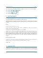
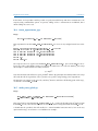
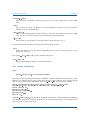
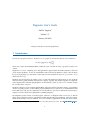
Flagmatic User’s Guide
Emil R. Vaughan∗
Version 1.5
January 29, 2012
A tool for researchers in extremal graph theory.
1
Introduction
Let H be an r-graph on h vertices. Then for a set of r-graphs F , the Turán H-density of F is defined as
n
πH (F ) = lim exH (n, F )/
,
n→∞
h
where exH (n, F ) is the maximum number of induced copies of H that an F -free r-graph on n vertices can
contain.
Flagmatic is a tool for computing exact and approximate upper bounds on Turán H-densities, and some
closely related problems. It uses the semi-definite method devised by Razborov, which comes from his
theory of flag algebras [9]. Expositions of this method can be found in Section 2 of [3], Section 7 of [7]
and Section 2.1 of [1].
Flagmatic was developed by the author as part of joint work with Victor Falgas-Ravry. It was originally
developed with 3-graphs in mind, although now 3-graphs, 2-graphs and oriented 2-graphs are supported.
Some original results obtained using Flagmatic can be found in [3] and [4]. The website contains a longer
list of results that it can prove.
Flagmatic is known to work on Linux and Mac OS X; although it will not take much work to get it running
on other operating systems. A semi-definite program (SDP) solver is required; it is recommended that this
be the SDP solver csdp. For the computation of exact bounds, the open source mathematics system Sage is
required. Section 4 details the requirements for running Flagmatic.
The Flagmatic system consists of a main program, referred to as ‘flagmatic’ with a lower-case ‘f’, and the
helper scripts. flagmatic produces approximate bounds using floating point arithmetic. The helper scripts,
which run under Sage’s version of Python, are used to turn these approximate bounds into exact bounds.
∗
School of Electronic Engineering and Computer Science, Queen Mary, University of London. Email: [email protected]
1
Flagmatic User’s Guide
version 1.5
By ‘exact bound’, we mean a bound that can be verified using only integer arithmetic. This process is
explained in Section 8.
Flagmatic is especially useful for computing quick approximate bounds. For example, let K4− be the unique
3-graph on 4 vertices with 3 edges. We can compute an approximate version of De Caen’s upper bound on
π(K4− ) [2] by running the flagmatic executable from the shell as follows:
$ ./flagmatic --r 3 --n 5 --forbid-k4- --dir output
flagmatic version 1.5
============================================================================
Forbidding 4.3
Using admissible graphs of order 5.
Generated 1 type of order 1, with 2 flags of order 3.
Generated 2 types of order 3, with [7, 4] flags of order 4.
Generated 11 admissible graphs.
Approximate floating point bound is 0.33333334
The --r 3 option tells flagmatic that we are working on a 3-graph problem, and the --n 5 option tells
flagmatic to use admissible graphs of order 5. The --forbid-k4- option specifies that K4− is to be
forbidden. The --dir option is mandatory, and specifies a directory in which to place the output files.
flagmatic creates several files inside this directory; these files are used by the helper scripts.
A better bound can be obtained by replacing --n 5 with --n 6 (or --n 7) at the expense of increasing
the time needed for the computation. Note that this bound is computed using floating point arithmetic,
and as such is approximately, but not exactly, equal to 1/3. In order to produce exact bounds it is necessary
to use the helper scripts—this is discussed in Section 8.
2
Support
The author is keen to hear reports of any bugs or installation difficulties. Comments or suggestions for
improvement are also very welcome! Please contact the developer by email at [email protected].
There is a website for Flagmatic, which can currently be found at
http://www.maths.qmul.ac.uk/~ev/flagmatic/
This will most likely change in the future, so please check before citing this address.
3
A note on graph notation
Flagmatic uses a simple format for specifying graphs. By ‘graph’, we mean one of the three kinds of graph
that Flagmatic supports; in other words, a ‘graph’ could be a 3-graph, a 2-graph or an oriented 2-graph.
Graphs are represented by a string consisting of the number of vertices, a colon ‘:’, and a list of edges.
Graphs on n vertices are always assumed to have vertices labelled 1, . . . , n. The number of vertices must
be between 0 and 9 inclusive. For example:
page 2 of 26
Flagmatic User’s Guide
version 1.5
4:123124134 is the 3-graph on 4 vertices with edges 123, 124 and 134,
4:121314 is the 2-graph (or oriented 2-graph) on 5 vertices with edges 12, 13 and 14, and
3: is the 3-graph (or 2-graph or oriented 2-graph) on 3 vertices with no edges.
The order in which the edges appear is not significant, and, with the exception of oriented graphs, the order
in which vertices appear within edges is not significant. For the most part, Flagmatic works with unlabelled
graphs, and so the actual way the vertices are labelled is not significant. In some cases, Flagmatic may
display graphs with a different labelling to that provided by the user.
The scripts check_construction.py and make_zero_eigenvectors.py also accept “degenerate
graphs”; these are graphs that contain edges with repeated vertices. For example, a degenerate 2-graph
may contain edges like 11, and a degenerate 3-graph may contain edges like 111 or 112. (Degenerate
edges are currently not allowed in oriented 2-graphs.)
Flagmatic also uses a variant of this notation to describe certain sets of graphs. The set of graphs on n
vertices that have exactly m edges is denoted by n.m. For example:
5.7 is the set of 3-graphs of order 5 that have 7 edges,
6.10 is the set of 3-graphs of order 6 that have 10 edges, and
4.0 is the set of 3-graphs (or 2-graphs or oriented 2-graphs) of order 4 that have no edges (of which
there is only one).
4
Requirements
flagmatic is written in C and should work on all POSIX compliant systems. (At least, this is the intention of
the author!) It has been tested on Linux and Mac OS X, and may work on Windows. The developer is keen
to hear from anyone who gets flagmatic running on Windows or other platforms.
An SDP solver is required. This can be csdp or sdpa (or any other SDP solver that accepts the “SDPA sparse”
format). csdp is currently the recommended SDP solver, and flagmatic will try to use it by default.
If using csdp, the csdp executable should be placed somewhere where flagmatic can find it. The easiest
way to do this is to place it in the same directory as flagmatic. (It can reside elsewhere if necessary; see
Section 5.)
The SDP solver sdpa can be used, albeit with slightly more effort on the part of the user. However, it tends
to find solutions whose kernels have higher dimension than those found by csdp. The author has observed
that csdp finds matrices whose kernel is as small as possible, given the constraints of the problem (although
he does not know why this is the case). When using sdpa, the make_zero_eigenvectors.py script may
fail to find a full set of zero eigenvectors. However, one reason why one may wish to use sdpa is that it has
high-precision versions that can be used to produce very accurate floating point solutions.
The helper scripts that are used for computing exact bounds require Sage. Sage should be installed so that
it can be run from the shell; this may require setting the PATH environment variable. Sage is not needed if
exact bounds are not required.
page 3 of 26
Flagmatic User’s Guide
version 1.5
csdp, sdpa, and Sage can be downloaded from the following places (links correct as of January 2012):
csdp : http://projects.coin-or.org/Csdp/
sdpa : http://sdpa.sourceforge.net/
Sage : http://www.sagemath.org/
5
Compiling flagmatic
It is recommended that Mac OS X users download the binary distribution from the Flagmatic website, which
comes with precompiled versions of the flagmatic executable and csdp.
Compiling the flagmatic executable is very easy; all that is needed is a C compiler. Linux users will most
likely already have one; Mac OS X users will need to install the Developer Tools. flagmatic can be compiled
by typing
$ make
In most cases, this is all that needs to be done.
Some users may wish to change the CFLAGS variable in the Makefile to control compiler options (for
example to turn on certain optimizations).
The helper scripts are written in Python, and do not need compiling.
flagmatic needs to run the csdp executable. When flagmatic is run, it will check whether the csdp executable is in the same directory as flagmatic, and if not, flagmatic will look in the directories listed in the
PATH environment variable. If you wish to keep the csdp executable somewhere else, then you must set
the CSDP environment variable to the filename of the csdp executable. For example, if the filename of the
csdp executable is /opt/bin/csdp, then to set the CSDP environment variable from the Bash shell you
can type:
$ export CSDP=/opt/bin/csdp
Note that if you set the CSDP environment variable, flagmatic will always try to use it, and will not look
anywhere else. If you wish to unset the CSDP environment variable, you can type:
$ unset CSDP
6
Compiling CSDP
Compiling csdp is somewhat more difficult, as it needs to be linked with the BLAS and LAPACK linear
algebra libraries. The developer of csdp provides binaries on his website. However, it is possible to achieve
page 4 of 26
Flagmatic User’s Guide
version 1.5
greater performance on Mac OS X by linking with the Accelerate Framework, and on Linux by linking with
the Intel Math Kernel Library.
Some instructions are provided below, but if you are having difficulty compiling csdp, please feel free to
contact the author at [email protected].
6.1
Mac OS X
The Mac OS X binary distribution of Flagmatic provides a csdp binary compiled using the following instructions,
so you may wish to download this if you use Mac OS X.
To build csdp version 6.1.1 on Mac OS X using the Accelerate Framework, download Csdp-6.1.1.tgz
and unpack the archive. Change to the lib directory and run make. Then change to the solver directory,
and in the Makefile change the line
LIBS=-L../lib -lsdp -llapack -lblas -lgfortran -lm
to
LIBS=-L../lib -lsdp -lm -framework Accelerate
Then run make, and the csdp executable will be created. This can then be moved somewhere where
flagmatic will find it.
6.2
Linux
The author suggests that Linux users link csdp with the Intel Math Kernel Library, which is free for noncommercial use, and can be downloaded from
http://software.intel.com/en-us/articles/non-commercial-software-download/
To build csdp version 6.1.1 on Linux using the Intel Math Kernel Library, download Csdp-6.1.1.tgz and
unpack the archive. Change to the lib directory and run make. Then change to the solver directory,
and in the Makefile change the line
LIBS=-L../lib -lsdp -llapack -lblas -lgfortran -lm
to
LIBS=-L/opt/intel-mkl-10.3/mkl/lib/ia32 -L../lib -lsdp -lmkl_intel -lmkl_sequential \
-lmkl_core -lpthread -lm
page 5 of 26
Flagmatic User’s Guide
version 1.5
where /opt/intel-mkl-10.3/ should be replaced with the directory into which you installed the Intel
Math Kernel Library. (You may also need to replace ia32 with something else if you are using 64-bit
Linux.) Then run make, and the csdp executable will be created. This can then be moved somewhere
where Flagmatic will find it.
You will need to set the LD_LIBRARY_PATH environment variable before csdp can run. From the Bash
shell you can type
export LD_LIBRARY_PATH=$LD_LIBRARY_PATH:/opt/intel-mkl-10.3/mkl/lib/ia32
Again, change /opt/intel-mkl-10.3/ to wherever you installed the Intel Math Kernel Library. It is
recommended that you put this command in your .bashrc file.
7
Examples: quick approximate bounds
The most basic way to use Flagmatic is to use it for computing approximate floating point bounds. We
shall assume that csdp is installed in a directory where flagmatic can find it (e.g. in the same directory as
flagmatic).
The examples in this section all concern 3-graphs. We can compute an approximate upper bound on π(K4− )
as follows:
$ ./flagmatic --r 3 --n 6 --forbid-k4- --dir output
flagmatic version 1.5
============================================================================
Forbidding 4.3
Using admissible graphs of order 6.
Generated 1 type of order 0, with 2 flags of order 3.
Generated 1 type of order 2, with 8 flags of order 4.
Generated 3 types of order 4, with [41, 26, 18] flags of order 5.
Generated 106 admissible graphs.
Approximate floating point bound is 0.29779503
Here, flagmatic has used csdp to produce an approximate bound. It is important to stress that this bound
is approximate, and cannot be considered entirely rigorous. The helper scripts can be used to make this
bound exact. Use of the helper scripts will be covered in Section 8.
The bound obtained is equal to that given by Razborov [10]. Because K4− is a graph often encountered in
extremal 3-graph theory, flagmatic has a special --forbid-k4- option to forbid K4− as a subgraph, which
we have used in the above example. We can also specify that we wish to forbid K4− by describing K4− in
Flagmatic’s graph notation:
$ ./flagmatic --r 3 --n 6 --forbid 4:123124134 --dir output
...
Approximate floating point bound is 0.29779503
(The ‘...’ indicates that some of the output has been omitted to save space.) The --n 6 option tells
flagmatic to use admissible graphs of order 6. If the option --n 7 is used, flagmatic will perform the
page 6 of 26
Flagmatic User’s Guide
version 1.5
computation using admissible graphs of order 7, which will give an improved bound, at the cost of taking
longer. (Most of the time will be spent running the SDP solver. The author has seen times of between
1.5 and 10 hours for the --n 7 computation; much depends on the hardware and which linear algebra
libraries csdp is linked with.)
The --verbose option can be used to enable verbose mode. In this mode, flagmatic will display slightly
more information, and in particular will display all the intermediate output from the SDP solver. The
--verbose option is especially recommended for --n 7 3-graph computations and --n 8 2-graph computations.
We can compute an approximate upper bound on π(K4 ), equal to one given by Razborov [10], as follows:
$ ./flagmatic --r 3 --n 6 --forbid-k4 --dir output
...
Approximate floating point bound is 0.56166560
We are not limited to forbidding one graph at a time; in fact any number of graphs may be forbidden. We
can compute an approximate upper bound on π(K4− , C5 ):
$ ./flagmatic --r 3 --n 6 --forbid-k4- --forbid-c5 --dir output
...
Approximate floating point bound is 0.25452806
The result is close to 1/4, which is the best lower bound known, and is conjectured [3] to be the true value
of π(K4− , C5 ). (Note that a slightly better bound can be obtained using --n 7.)
We can compute an approximate upper bound on π(5.7, induced 5.5). (This means that 5-vertex subgraphs are forbidden from spanning 5 or at least 7 edges.)
$ ./flagmatic --r 3 --n 6 --forbid 5.7 --forbid-induced 5.5 --dir output
...
Approximate floating point bound is 0.46453411
p
The result is close to the best known lower bound, of 2 3 − 3 ≈ 0.464101, given by a construction of
Mubayi and Rödl [8].
8
Examples: exact bounds
In the previous section, we looked at some examples of using flagmatic to produce approximate floating
point bounds. The Flagmatic suite comes with some helper scripts, which can be used to turn an approximate bound into an exact bound. There are two ways to do this: the first is for problems where the bound
appears to be tight, and where the problem admits a blow-up construction as its stable extremal example.
The second method can be used in all situations, but does not lead to tight bounds.
In this section, three examples are presented. More examples can be found on the Flagmatic website, and
each example on the website has a link to a “transcript” that gives the sequence of commands necessary
for reproducing the result.
page 7 of 26
Flagmatic User’s Guide
version 1.5
flagmatic
check_construction.py
find_sharp_graphs.py
make_zero_eigenvectors.py
make_nontight_exact_qdash.py
factor_approximate_q.py
make_exact_qdash.py
verify_bound.py
make_certificate.py
inspect_certificate.py
Figure 1: The helper scripts poset.
With the exception of the stand-alone check_construction.py script, the helper scripts must be run
in the order shown Figure 1. (Note that below flagmatic there are two choices, corresponding to the two
methods of producing exact results.)
The script inspect_certificate.py is also somewhat independent of the others. It is provided with
the Flagmatic suite, but is also available separately, and does not depend on any other parts of Flagmatic.
Its job is to extract information from the certificates made by make_certificate.py.
As a first example, let us determine the exact value of π(K4 , induced 4.1), a result due to Razborov [10].
A lower bound of 5/9 ≤ π(K4 , induced 4.1) is given by Turán’s construction, a blow-up of the graph
3:123112223331. We run flagmatic as follows:
$ ./flagmatic --r 3 --n 6 --forbid-k4 --forbid-induced 4.1 --dir output
flagmatic version 1.5
============================================================================
Forbidding 4.4
Forbidding 4.1 as an induced subgraph.
Using admissible graphs of order 6.
Generated 1 type of order 0, with 2 flags of order 3.
Generated 1 type of order 2, with 8 flags of order 4.
Generated 3 types of order 4, with [15, 15, 17] flags of order 5.
Generated 34 admissible graphs.
Approximate floating point bound is 0.55555556
So flagmatic has produced a floating point upper bound, which looks very much like it should be 5/9. But
at this stage the bound is only approximate.
We can now use the helper scripts to turn the floating point bound into an exact bound. The next step is
to identify which graphs are sharp. To do this, we run the find_sharp_graphs.py script:
page 8 of 26
Flagmatic User’s Guide
version 1.5
$ sage -python scripts/find_sharp_graphs.py --dir output
Floating point bound is 0.555555557483315088.
8 members of H are sharp.
0.555555554189191003 : graph 1 (6:)
0.555555556177857124 : graph 2 (6:123124125126)
0.555555556613102297 : graph 10 (6:123124125136146156236246256)
0.555555557193247784 : graph 11 (6:123124125126134135136145146156)
0.555555557483226936 : graph 23 (6:123124125126134135136145146256356456)
0.555555556178151999 : graph 26 (6:123124125134135145236246256346356456)
0.555555557483315088 : graph 31 (6:123124125126134135136245246256345346356)
0.555555557048232007 : graph 34 (6:123124125134135146156236245246256345346356)
Written sharp graphs to flags.py
The lower bound is given by a blow-up of 3:123112223331. So if all is well, the admissible graphs that
are sharp should be the graphs that occur as 6-vertex induced subgraphs of blow-ups of 3:123112223331.
We run check_construction.py as follows:
$ sage -python scripts/check_construction.py --r 3 3:123112223331 --n 6
Density is 5/9.
8 graphs of order 6 occur as induced subgraphs of the blow-up:
6: has density 7/243 (0.028807)
6:123124125126 has density 5/81 (0.061728)
6:123124125136146156236246256 has density 20/243 (0.082305)
6:123124125126134135136145146156 has density 4/27 (0.148148)
6:123124125126134135136145146256356456 has density 20/81 (0.246914)
6:123124125134135145236246256346356456 has density 5/81 (0.061728)
6:123124125126134135136245246256345346356 has density 20/81 (0.246914)
6:123124125134135146156236245246256345346356 has density 10/81 (0.123457)
This is good: the two lists of graphs are the same! This means that we can be confident of getting an exact
result.
Next, we run the script make_zero_eigenvectors.py, which will use the graph 3:123112223331,
an extremal construction for the problem, to construct a full set of zero eigenvectors of the floating point
matrices Q found by flagmatic. Because 3:123112223331 is vertex transitive, we can use the option
--vertex-transitive to speed the computation up a little bit.
$ sage -python scripts/make_zero_eigenvectors.py 3:123112223331
--vertex-transitive --dir output
Constructed 1 out of 1 zero eigenvectors for type 1.
Constructed 3 out of 3 zero eigenvectors for type 2.
Constructed 5 out of 5 zero eigenvectors for type 3.
Constructed 1 out of 1 zero eigenvectors for type 4.
Constructed 4 out of 4 zero eigenvectors for type 5.
Written zev.py
Written field to flags.py
We now have a complete set of zero eigenvectors. The next step is to run factor_approximate_q.py,
which will factor each of the matrices Q as Q = R Q0 R T , where Q0 is a positive definite matrix.
page 9 of 26
Flagmatic User’s Guide
version 1.5
$ sage -python scripts/factor_approximate_q.py --dir output
Floating point bound is 0.555555557483314866.
Type 1: smallest eigenvalue is 0.180758628947732980
Type 2: smallest eigenvalue is 0.025204209832725446
Type 3: smallest eigenvalue is 0.127913863682220269
Type 4: smallest eigenvalue is 0.116791535663077511
Type 5: smallest eigenvalue is 0.099219286066487625
Written r.py
Written qdashf.py
Next we run the make_exact_qdash.py script to create exact versions of the matrices Q0 from the
floating point versions. It is necessary to provide the script with the bound we are trying to obtain, in this
case 5/9.
$ sage -python scripts/make_exact_qdash.py 5/9 --dir output
Type 1: smallest eigenvalue is 0.180766796512166816
Type 2: smallest eigenvalue is 0.025241578508074593
Type 3: smallest eigenvalue is 0.127913796971273697
Type 4: smallest eigenvalue is 0.116823645035926724
Type 5: smallest eigenvalue is 0.099219353648207789
Written qdash.py
Added exact bound to flags.py
Finally, we run the verify_bound.py script to see if the exact bound has been achieved (there are a few
things that can go wrong, so this step is essential):
$ sage -python scripts/verify_bound.py --dir output
Written q.py
Floating point bound (non-sharp graphs) is 0.554201367482783369
Exact bound (just sharp graphs) is 5/9
Bound (all graphs) is 5/9
Now we definitely have the exact result. The last thing to do is to run make_certificate.py to produce
a certificate in JSON (a widely-used lightweight data-interchange format), which can be verified by others:
$ sage -python scripts/make_certificate.py --dir output
Written certificate to cert.js
The certificate contains details of the problem, the forbidden subgraphs, the admissible graphs, types and
flags, and the Q0 and R matrices. The Q matrices can be computed as Q = R Q0 R T . The reason for providing
the Q0 matrices, rather than the Q matrices, is that while the Q matrices are positive semi-definite, the Q0
matrices are positive definite. Positive definiteness is easier to verify than positive semi-definiteness, for
example by checking that the principal minors are all positive (Sylvester’s criterion). Note that if Q0 is
positive definite, then for any (row) vector x,
x Q x T = x (R Q0 R T ) x T = (x R) Q0 (x R) T ≥ 0,
and so Q is positive semi-definite.
Next, we shall look at how we can obtain a result for 2-graphs, due to Grzesik [5] and independently
Hatami, Hladký, Král, Norine and Razborov [6]. The result is that a triangle-free 2-graph can have a
C5 -density of at most 24/625. The process is extremely similar to the one we used for the previous result.
page 10 of 26
Flagmatic User’s Guide
version 1.5
We begin by running flagmatic. Notice that we can forbid triangles by using the option --forbid 3.3 (alternatively we could use --forbid 3:122331), and we use the --induced-density option to specify
that we want to maximise the C5 -density.
$ ./flagmatic --r 2 --n 5 --induced-density 5:1223344551 --forbid 3.3 --dir output
flagmatic version 1.5
============================================================================
Optimizing for density of 5:1213243545.
Forbidding 3.3
Using admissible graphs of order 5.
Generated 1 type of order 1, with 5 flags of order 3.
Generated 3 types of order 3, with [8, 6, 5] flags of order 4.
Generated 14 admissible graphs.
Approximate floating point bound is 0.03840000
As before, we next run the find_sharp_graphs.py script:
$ sage -python scripts/find_sharp_graphs.py --dir output
Floating point bound is 0.038400000791913261.
10 members of H are sharp.
0.038399999866059319 : graph 1 (5:)
0.038399999179418200 : graph 2 (5:12)
0.038400000469420784 : graph 3 (5:1213)
0.038400000146933733 : graph 5 (5:121314)
0.038400000630675675 : graph 8 (5:12131415)
0.038400000791913212 : graph 9 (5:12131425)
0.038399999824450450 : graph 10 (5:12132434)
0.038400000791913261 : graph 12 (5:1213142535)
0.038399999501926962 : graph 13 (5:1213243545)
0.038400000727425887 : graph 14 (5:121314253545)
Written sharp graphs to flags.py
A blow-up of C5 , or 5:1223344551 in Flagmatic’s notation, is known to be extremal for this problem. We
can now verify that the sharp graphs are those that we would expect to occur if the bound is tight:
$ sage -python scripts/check_construction.py --n 5 --r 2 5:1223344551
--vertex-transitive --induced-density 5:1223344551
Density of 5:1223344551 is 24/625.
10 graphs of order 5 occur as induced subgraphs of the blow-up:
5: has density 31/625 (0.049600)
5:12 has density 4/125 (0.032000)
5:1213 has density 12/125 (0.096000)
5:121314 has density 8/125 (0.064000)
5:12132434 has density 6/125 (0.048000)
5:12131425 has density 24/125 (0.192000)
5:12131415 has density 16/125 (0.128000)
5:1213243545 has density 24/625 (0.038400)
5:1213142535 has density 24/125 (0.192000)
5:121314253545 has density 4/25 (0.160000)
Everything seems in order, so we can now construct the zero eigenvectors:
page 11 of 26
Flagmatic User’s Guide
version 1.5
$ sage -python scripts/make_zero_eigenvectors.py 5:1223344551
--vertex-transitive --dir output
Constructed 1 out of 1 zero eigenvectors for type 1.
Constructed 4 out of 4 zero eigenvectors for type 2.
Constructed 1 out of 1 zero eigenvectors for type 3.
Constructed 2 out of 2 zero eigenvectors for type 4.
Written zev.py
Written field to flags.py
We now factor the Q matrices:
$ sage -python scripts/factor_approximate_q.py --dir output
Floating point bound is 0.038400000791913261.
Type 1: smallest eigenvalue is 0.020312545339158966
Type 2: smallest eigenvalue is 0.148959264212904008
Type 3: smallest eigenvalue is 0.176046112223611911
Type 4: smallest eigenvalue is 0.445612724880143529
Written r.py
Written qdashf.py
And produce exact versions of the Q0 matrices:
$ sage -python scripts/make_exact_qdash.py 24/625 --dir output
Type 1: smallest eigenvalue is 0.020312572324406988
Type 2: smallest eigenvalue is 0.148971226934540624
Type 3: smallest eigenvalue is 0.176008173330834516
Type 4: smallest eigenvalue is 0.445611441081160908
Written qdash.py
Added exact bound to flags.py
We verify the bound:
$ sage -python scripts/verify_bound.py --dir output
Written q.py
Floating point bound (non-sharp graphs) is 0.033726805738722151
Exact bound (just sharp graphs) is 24/625
Bound (all graphs) is 24/625
Finally, we make a certificate:
$ sage -python scripts/make_certificate.py --dir output
Written certificate to cert.js
As a final example, we shall look at a bound that is not tight. In the previous section, we saw that we can
compute an approximate upper bound on π(K4 ), equal to one given by Razborov [10]:
page 12 of 26
Flagmatic User’s Guide
version 1.5
$ ./flagmatic --r 3 --n 6 --forbid-k4 --dir output
flagmatic version 1.5
============================================================================
Forbidding 4.4
Using admissible graphs of order 6.
Generated 1 type of order 0, with 2 flags of order 3.
Generated 1 type of order 2, with 11 flags of order 4.
Generated 4 types of order 4, with [64, 56, 50, 45] flags of order 5.
Generated 964 admissible graphs.
Approximate floating point bound is 0.56166560
The best-known lower bounds give us 5/9—for example Turán’s construction—so we are not going to be
able to get a tight bound here. However, we can still prove an exact upper bound. We run the script
make_nontight_exact_qdash.py to produce rational R and Q0 matrices:
$ sage -python scripts/make_nontight_exact_qdash.py --dir output
Written r.py
Written qdash.py
Marked bound as non-tight in flags.py
Finally, we run the verify_bound.py script. In this case, the exact bound is printed:
$ sage -python scripts/verify_bound.py --dir output
Written q.py
Bound (all graphs) is 2246662543771/4000000000000
(Approximately 0.561665636)
Added exact bound to flags.py
Note that the script prints out a decimal approximation to the exact bound, as well as the exact bound.
But just to be clear: the exact bound is the rational number given first. As before, we can use the script
make_certificate.py to produce a certificate of the result:
$ sage -python scripts/make_certificate.py --dir output
Written certificate to cert.js
9
flagmatic command-line options
flagmatic should be run from the shell prompt as follows:
$ ./flagmatic --n INTEGER --dir DIRECTORY OPTIONS
All options are prefixed by two hyphens. The --n and --dir options are mandatory; all others are
optional. The following is a complete list of options available.
Note that the --forbid, --forbid-induced, --sharp and --induced-density options may be used
multiple times.
page 13 of 26
Flagmatic User’s Guide
version 1.5
--n INTEGER (required) This sets the number of vertices of the admissible graphs. Currently values
between 4 and 7 (inclusive) are supported for 3-graphs, and between 3 and 8 (inclusive) for 2graphs.
--dir DIRECTORY (required) This sets the directory that will be used to store the output files. (If
DIRECTORY is ‘.’ then the current directory is used.)
--r INTEGER Specifies that r-graphs should be used. The default value is 3.
--oriented Specifies that oriented graphs should be used. Currently this option is only allowed when
using --r 2.
--induced-density GRAPH Specifies that we want to optimize the density of GRAPH, rather than edge
density. Can be used multiple times.
--forbid GRAPH Specifies a graph to forbid as a subgraph. Can be used multiple times.
--forbid-induced GRAPH Specifies a graph to forbid as an induced subgraph. Can be used multiple
times.
--sharp GRAPH Constrains the SDP to be sharp on the given graph. Can be used multiple times.
--nosolve Do not run the SDP solver csdp; just set up the SDP program and quit. This option is useful if
one wants to use sdpa or another SDP solver, and to not have csdp run.
--verbose If this option is given, more information about the computation will be given, as well as the
output from the SDP solver. Use of this option is recommended for long computations, for example
when using --n 7.
--minimize If this option is given, the minimum density will be found instead of the maximum density.
--max-flags NUM Exclude types that have more than NUM flags.
--exclude-type NUM Exclude type number NUM.
The following options are available, for conveniently forbidding popular 3-graphs.
--forbid-k4- Forbids graphs that contain the unique graph of order 4 with three edges, often called
K4− . (Called G3 in [10].) Equivalent to --forbid 4.3.
--forbid-k4 Forbids graphs that contain the unique graph of order 4 with four edges, K4 . (Called G4 in
[10].) Equivalent to --forbid 4.4.
--forbid-k5 Forbids graphs that contain the unique graph of order 5 with ten edges, K5 . Equivalent to
--forbid 5.10.
--forbid-c5 Forbids C5 , the graph on 5 vertices with edges 123, 234, 345, 451 and 512. Equivalent to
--forbid 5:123234345451512.
--forbid-f32 Forbids F3,2 , the graph on 5 vertices with edges 123, 145, 245 and 345. Equivalent to
--forbid 5:123145245345.
page 14 of 26
Flagmatic User’s Guide
10
version 1.5
Helper scripts
The helper scripts are in the scripts directory of the Flagmatic distribution. If Sage has been installed,
and the PATH environment variable has been set correctly, then a helper script can be run under Sage’s
version of Python by entering something like the following at the shell prompt:
$ sage -python scripts/SCRIPT OPTIONS
The scripts find_sharp_graphs.py, check_construction.py, make_certificate.py, as well as
convert_sdpa_output.py do not in fact require Sage’s Python, and can be run by the standard Python
interpreter (version 2.6 or above).
The script inspect_certificate.py can also be run using the standard Python interpreter for certificates that do not use irrational numbers. For certificates that use irrational numbers, this script must be
run with Sage’s Python. In fact, it is recommended that Sage’s Python be used whenever possible, as the
script generally runs faster with Sage.
All other scripts require Sage’s Python.
Most of the scripts require a directory to be specified using the --dir option. This should be a directory
that was previously given to flagmatic with the --dir option, and that is populated with files generated
by flagmatic and the other scripts.
All of the scripts accept the --verbose option, which will cause more information to be displayed.
10.1
find_sharp_graphs.py
Usage:
find_sharp_graphs.py --dir DIRECTORY [--tolerance NUMBER] [--verbose]
This script should be run after flagmatic. It identifies which admissible graphs are sharp, and the sharp
graphs found are appended to the flags.py file in the directory specified.
If the result is exact, all the admissible graphs that occur as induced subgraphs of an extremal construction
will be sharp. (The script check_construction.py can be used to display which admissible graphs
occur as induced subgraphs of an extremal construction.)
For example:
$ sage -python scripts/find_sharp_graphs.py --dir output
Floating point bound is 0.222222222873386444.
3 members of H are sharp.
0.222222222873386444 : graph 1 (5:)
0.222222222726874252 : graph 5 (5:123124125)
0.222222222864506269 : graph 7 (5:123124135145)
Written sharp graphs to flags.py
page 15 of 26
Flagmatic User’s Guide
version 1.5
Note: If flagmatic was invoked with the --sharp option, one or more graphs may already be marked as
being sharp. In this case, the script will only write to flags.py if it finds any additional sharp graphs.
(The --sharp option is rarely useful; it is not needed for most problems.)
It is possible that in certain situations the script will incorrectly consider graphs to be sharp. One may
suspect this is happening if sharp graphs are found that do not occur as induced subgraphs of an extremal
construction. To rectify this, the --tolerance option can be used to specify a tolerance smaller than the
default value of 0.00001. For example:
$ sage -python scripts/find_sharp_graphs.py --dir output --tolerance 0.0000005
10.2
check_construction.py
Usage:
check_construction.py --r INTEGER --n INTEGER [--induced-density GRAPH]
[--vertex-transitive] [--verbose]
Given a graph, and a number of vertices specified with the --n option, this script considers blow-ups of
the graph, and determines which graphs on the given number of vertices can occur as induced subgraphs.
The kind of graph is specified with the --r option. Currently only 3-graphs and 2-graphs are supported;
oriented 2-graphs are not (currently) supported. The default value is 3.
Note that a directory should not be specified. This script is stand-alone; it merely provides the user with
information.
For example:
$ sage -python scripts/check_construction.py --r 3 3:123 --n 5
Density is 2/9.
3 graphs of order 5 occur as induced subgraphs of the blow-up:
5: has density 31/81 (0.382716)
5:123124125 has density 20/81 (0.246914)
5:123124135145 has density 10/27 (0.370370)
The script prints the (asymptotic) density of a blow-up, and all graphs of order 5 that can occur as induced
subgraphs.
Input graphs are allowed to contain “degenerate” edges. For example, a complete bipartite 3-graph can
be represented by 2:112122 (this graph has two parts of equal size, and all possible edges that are not
entirely contained within one part).
sage -python scripts/check_construction.py --r 3 2:112122 --n 5
Density is 3/4.
3 graphs of order 5 occur as induced subgraphs of the blow-up:
5: has density 1/16 (0.062500)
5:123124125134135145 has density 5/16 (0.312500)
5:123124125134135145234235245 has density 5/8 (0.625000)
page 16 of 26
Flagmatic User’s Guide
version 1.5
If the graph is vertex transitive, a small speed gain can be had by using the --vertex-transitive
option. Note that the script does not check that the graph is indeed vertex transitive; if it is not, the results
will be wrong.
The option --induced-density can be used to report the density of a certain graph on the first line of
output, rather than the edge density.
10.3
make_zero_eigenvectors.py
Usage:
make_zero_eigenvectors.py GRAPH --dir DIRECTORY [--vertex-transitive]
[--zero-threshold NUMBER] [--verbose]
This script must be run after find_sharp_graphs.py. A graph must be provided, which should be a
(conjectured) extremal construction for the problem. The script computes asymptotic flag densities in a
blow-up of the graph provided, in order to find zero eigenvectors of the positive semi-definite matrices
found by the SDP solver. These zero eigenvectors are placed in the zev.py file. For example:
$ sage -python scripts/make_zero_eigenvectors.py 3:122123133 --dir output
Constructed 1 out of 1 zero eigenvectors for type 1.
Constructed 4 out of 4 zero eigenvectors for type 2.
Constructed 6 out of 6 zero eigenvectors for type 3.
Constructed 1 out of 1 zero eigenvectors for type 4.
Constructed 1 out of 1 zero eigenvectors for type 5.
Written zev.py
If the graph is not an extremal construction, a full set of eigenvectors will most probably not be found, and
the script will exit with an error message.
In the case that the extremal graph is vertex transitive, the script can be made to run slightly faster by
using the --vertex-transitive option. This option should be used with care, as the script does not
verify that the graph provided is indeed vertex transitive. If it is not, the script may fail to find all the zero
eigenvectors.
As with check_construction.py, graphs with degenerate edges can be provided.
Note that check_construction.py will show that the graphs 2:112 and 3:122123133 have the same
set of induced subgraphs of order n, for any n. However, these graphs are quite different as far as
make_zero_eigenvectors.py is concerned. Blow-ups of both graphs consist of two parts 1 and 2,
which all possible edges of the form 112. But the asymptotic flag densities are different.
The option --zero-threshold can be used to alter the threshold at which the script considers an eigenvalue to be zero. It is set by default to a value that works for almost all problems, when using csdp.
The script also allows a few “ad hoc” constructions, that do not arise from blow-ups. These can be accessed
by specifying the special keywords maxs3, maxs4 or max42, instead of giving a graph. These are used in
the problems of maximizing the induced densities of the oriented 2-graphs S3 and S4 and of the 3-graph
4.2—see the transcripts on the website for how these are used.
page 17 of 26
Flagmatic User’s Guide
version 1.5
In the future, it is hoped that it will be possible to specify iterated blow-up and other constructions to the
script by using command-line options. At present, adding “ad hoc” constructions is not difficult, but it
entails editing the source code.
10.4
factor_approximate_q.py
Usage:
factor_approximate_q.py --dir DIRECTORY [--verbose]
This script must be run after make_zero_eigenvectors.py. Its use is very straight-forward. For example:
$ sage -python scripts/factor_approximate_q.py --dir output
Floating point bound is 0.222222222873387026.
Type 1: smallest eigenvalue is 3.184802519668853638
Type 2: smallest eigenvalue is 0.326187267853862428
Type 3: smallest eigenvalue is 0.254045018479330809
Written r.py
Written qdashf.py
The script uses the zero eigenvectors that make_zero_eigenvectors.py places in the zev.py file to
factor the positive semi-definite matrices Q found by the SDP solver. For each such matrix Q, this script
will attempt to construct matrices R and Q0 such that
Q = R Q0 R T .
Note that the matrices R will not be square, and RR T will not (in general) be the identity matrix. The script
will verify that all the eigenvalues of the Q0 matrices are positive, using floating point computations.
The R matrices are written to the r.py file, and the Q0 matrices, which are still floating point at this stage,
are written to the qdashf.py file.
10.5
make_exact_qdash.py
Usage:
make_exact_qdash.py BOUND --dir DIRECTORY [--denominator INTEGER]
[--diagonalize] [--verbose]
This script must be run after factor_approximate_q.py. It takes the floating point Q0 matrices from
the qdashf.py file, and converts them into an exact form, before saving them in the the qdash.py file.
A bound must be provided; this will usually be a rational number between 0 and 1, but can be any
expression that Sage can evaluate to a real number. For example:
page 18 of 26
Flagmatic User’s Guide
version 1.5
$ sage -python scripts/make_exact_qdash.py 2/9 --dir output
Type 1: smallest eigenvalue is 3.184807256235827833
Type 2: smallest eigenvalue is 0.326187199999999677
Type 3: smallest eigenvalue is 0.254045000000000021
Written qdash.py
Added exact bound to flags.py
This script converts the Q0 matrices in such a way that the bound provided is attained. The script then
computes the eigenvalues, which will be close to those reported by the factor_approximate_q.py
script, but will typically be slightly different. The eigenvalue computation is done using floating point
arithmetic, and as such is not entirely rigorous.
If the --diagonalize option is specified, the script will modify the R and Q0 matrices so that the Q0
matrices are diagonal matrices with positive entries. In this case, the positive definiteness of the Q0 matrices
is trivial to verify. However, using this option can significantly increase the time and memory requirements
of the script.
An optional number can be provided with --denominator. This specifies the denominator to use when
converting floating point entries into rational numbers. For example:
$ sage -python scripts/make_exact_qdash.py 2/9 --dir output --denominator 6
If the number given is too low, the exact Q0 matrices may have negative eigenvalues and the script will
exit with an error. In this case, the script should be rerun and a higher denominator specified. The default
denominator is 10000000, which is enough for most purposes.
If you wish to produce “pretty” matrices, then you should try choosing denominators that are as low as
possible.
10.6
make_nontight_exact_qdash.py
Usage:
make_nontight_exact_qdash.py --dir DIRECTORY [--denominator INTEGER]
[--ldl] [--verbose]
This script is for the computation of bounds that are not tight. (It can in fact be used in any situation, but
it will not give tight bounds.) It should be run after flagmatic.
The script uses numerical Cholesky decomposition, followed by rounding, to produce the R and Q0 matrices.
The Q0 matrices produced are identity matrices.
For example:
$ sage -python scripts/make_nontight_exact_qdash.py --dir output
Written r.py
Written qdash.py
Marked bound as non-tight in flags.py
page 19 of 26
Flagmatic User’s Guide
version 1.5
The --denominator option can be used, as with make_exact_qdash.py.
Sometimes the Cholesky decomposition fails, because there are eigenvalues indistinguishable from zero
(as opposed to being very small, as would normally be the case for ‘zero’ eigenvalues). In this case the
--ldl option can be used, which tells the script to perform an LDL decomposition instead of a Cholesky
decomposition. Note that the default Cholesky decomposition should be used whenever possible, as it
generally gives a sharper bound. Also, if LDL decomposition is used, the Q0 matrices will not be identity
matrices.
10.7
verify_bound.py
Usage:
verify_bound.py --dir DIRECTORY [--verbose]
This script verifies exact bounds, and it should be run after either make_exact_qdash.py or
make_nontight_exact_qdash.py. For example:
$ sage -python scripts/verify_bound.py --dir output
Written q.py
Floating point bound (non-sharp graphs) is 0.209855850616606526
Exact bound (just sharp graphs) is 2/9
Bound (all graphs) is 2/9
The script first does a floating point computation on all non-sharp graphs, which gives a quick indication of
whether the bound is valid. Then the sharp graphs are checked, with an exact computation, and finally all
the graphs are checked with an exact computation. The last check can sometimes take quite a long time,
which is why the first two checks are carried out.
Note: this script trusts (amongst other things) that flagmatic has determined a correct set of admissible
graphs, types and flags, and that the Q0 matrices provided are positive definite. So use of this script cannot
be regarded as an independent confirmation of a result.
It can sometimes happen that verify_bound.py shows that the bound has not been obtained. This
can happen when the rounding process perturbs the matrices enough to make the non-sharp graphs exceed the bound. If this happens, the script make_exact_qdash.py should be run again, with a larger
--denominator. If the --diagonalize option was used previously, it will also be necessary to re-run
the factor_approximate_q.py script to recover the original R matrices.
10.8
make_certificate.py
Usage:
make_certificate.py --dir DIRECTORY [--pair-densities] [--verbose]
page 20 of 26
Flagmatic User’s Guide
version 1.5
This script must be run after verify_bound.py. It produces a certificate in JSON format, cert.js. The
intention is that other programs can use the information contained within the certificate to perform an
independent check of Flagmatic’s computation.
The file contains an object with the following keys. Much of the data consists of numbers. In the case that
a number is an integer, it is given as an integer; if not, it is given as a string. For example, 1 is given as 1,
but 1/2 is given as "1/2".
Matrices are given as arrays of arrays of numbers, in row-major order. The Q0 matrices are symmetric, and
only the upper-triangle of each matrix is given. For example, if a Q0 matrix is the 3 × 3 identity matrix, it
will be given as
[[1,0,0], [1,0], [1]]
The R matrices are not necessary square; the whole of each matrix is given, in row-major order. For
example,
[[1,-2],[-5,3]]
represents the the matrix
1
−5
−2
.
3
Note that the Q matrices can be computed as Q = R Q0 R T .
description
String. An English description of the problem.
bound
Number. The bound.
order_of_admissible_graphs
Integer. The order of the admissible graphs.
number_of_admissible_graphs
Integer. The number of admissible graphs.
admissible_graphs
Array of strings. The admissible graphs in Flagmatic’s graph notation.
admissible_graph_densities
Array of numbers. The densities of each admissible graph. Uses the same ordering of admissible
graphs as the admissible_graphs array.
number_of_types
Integer. The number of types.
types
Array of strings. The types in Flagmatic’s graph notation.
page 21 of 26
Flagmatic User’s Guide
version 1.5
numbers_of_flags
Array of integers. The number of flags for each type. Uses the same ordering of types as the types
array.
flags
Array of arrays of strings. The flags for each type in Flagmatic’s graph notation. Uses the same
ordering of types as the types array.
qdash_matrices
Array of upper-triangular matrices. The Q0 matrices. Uses the same ordering of types as the types
array. If a type is not needed, then the corresponding array entry will be null.
r_matrices
Array of matrices. The R matrices. If an entry is null, then for this type, Q = Q0 .
If a field other than the rationals is used, then the following will be present:
field
String. The field used, together with an embedding into the reals, as a Sage expression. If not
present, the field is Q.
If the option --pair-densities is given, then there will also be:
pair_densities
Array of upper-triangular matrices. The flag-pair densities.
10.9
inspect_certificate.py
Usage:
inspect_certificate.py CERTIFICATE [OPTION]
This script can be used to display information contained in a certificate. Unlike the other scripts, the actual
filename of a certificate must be given, rather than a directory. (The certificate can be compressed with
‘gzip’ or ‘bzip2’—if this is done, the filename must end in .gz or .bz2 respectively.) For example:
$ sage -python scripts/inspect_certificate.py output/cert.js --verify-bound
Problem is "3-graph; maximize 3:123 density; forbid 5:123124125345".
Claimed bound is 4/9.
Computing Q matrices...
Computing pair densities...
Computing bound...
Bound is 4/9.
If inspect_certificate.py is run with no arguments apart from the certificate filename, it will display
some information about the certificate. Alternatively, one of the following options can be given (note that
only one option at a time can be used):
page 22 of 26
Flagmatic User’s Guide
version 1.5
--help Display list of options.
--admissible-graphs Display a list of admissible graphs in Flagmatic’s graph notation.
--flags Display a list of types and flags, all given in Flagmatic’s graph notation.
--r-matrices Display a list of the R matrices.
--qdash-matrices Display a list of the Q0 matrices.
--q-matrices Compute and display a list of the Q matrices.
--pair-densities Compute and display all the flag pair densities.
--verify-bound Verify the bound, by computing the Q matrices and flag pair densities, and performing
the required computations. Note that this is not a complete verification, as it does not check that the
list of admissible graphs is exhaustive.
--sharp-graphs Display a list of the admissible graphs that are sharp.
--flag-algebra-coefficients Display a list of the admissible graphs along with their flag algebra
coefficients.
If a certificate contains irrational numbers, then the script must be run under Sage’s version of Python,
otherwise the standard Python interpreter (2.6 or above) can be used. It is recommended that Sage’s
Python be used whenever possible, as the script generally runs faster with Sage.
10.10
make_sdpa_output.py
Usage:
make_sdpa_output.py INPUT OUTPUT
This script allows use of the SDP solver sdpa, instead of csdp. It converts an output file created by sdpa
into a csdp-style output format that the other helper scripts expect. (It does not produce a complete csdp
output file; it only produces the part that is used by the helper scripts.)
If one wishes to use sdpa instead of csdp, then flagmatic can be run with the --nosolve option, in order
to prevent csdp from being run. For example:
$ ./flagmatic --r 2 --oriented --n 4 --induced-density 3:1213 --dir output --nosolve
flagmatic version 1.5
============================================================================
Optimizing for density of 3:1213.
Using admissible graphs of order 4.
Generated 1 type of order 0, with 2 flags of order 2.
Generated 2 types of order 2, with [9, 9] flags of order 3.
Generated 42 admissible graphs.
page 23 of 26
Flagmatic User’s Guide
version 1.5
sdpa can then be run:
$ ./sdpa -ds output/flags.dat-s -o output/sdpa.out
...
Then the convert_sdpa_output.py script can be run to convert the output:
$ sage -python scripts/convert_sdpa_output.py output/sdpa.out output/flags.out
It is important that the output file be called flags.out, as this is what the helper scripts expect to find.
11
Files
Flagmatic creates some files in the directory specified by the mandatory --dir option.
flags.dat-s This is the input file for the SDP solver, in “SDPA sparse” format. This format is accepted by
csdp and sdpa. This file can be compressed using gzip to save space; if this is done, the compressed
version should be called flags.dat-s.gz. (Note that while the helper scripts can read compressed
files, csdp cannot, and so it should only be compressed after the SDP solver has been run.)
flags.rat This contains much the same information as flags.out, but the numbers are given as exact
rationals, rather than in decimal form. This file can be compressed using gzip to save space—if this
is done, the compressed version should be called flags.rat.gz.
flags.out When flagmatic runs csdp, the solution found by csdpis written to this file. If csdp is run
manually, the solution should be stored in flags.out so the helper scripts can find it. This file can
be compressed using gzip to save space; if this is done, the compressed version should be called
flags.out.gz.
flags.py Python source code; contains some information about the problem, including the admissible
graphs, types and flags.
In addition, the helper scripts create the following files.
zev.py Created by make_zero_eigenvectors.py. Python source code. Contains zero eigenvectors of
the Q matrices, found by the SDP solver. The entries are string representations of numbers.
r.py Created by factor_approximate_q.py or make_nontight_exact_qdash.py. Python source
code. Contains, for each type, a matrix R. The entries are string representations of rational numbers.
This file is overwritten by make_exact_qdash.py if the --diagonalize option is used.
qdashf.py Created by factor_approximate_q.py. Python source code. Contains, for each type, a
positive definite floating point matrix Q0 , such that Q = R Q0 R T .
qdash.py Created by make_exact_qdash.py or make_nontight_exact_qdash.py. Python source
code. Contains, for each type, a positive definite matrix Q0 . The entries are string representations of
numbers.
page 24 of 26
Flagmatic User’s Guide
version 1.5
q.py Created by verify_bound.py. Python source code. Contains, for each type, a matrix Q. The
entries are string representations of numbers.
cert.js JSON format. Contains a certificate of the solution. Created by make_certificate.py.
The .pyc versions of these files may also be present in the directory; these are created by the Python
interpreter.
12
Redistribution of flagmatic
There are no restrictions on the use of flagmatic, and no license is required to use it.
The developer grants the right of redistribution of the software under the conditions of the following
license (based on the 2-clause BSD license). To summarize, redistribution in source and binary form, with
or without modification, is permitted, but credit must be given.
Copyright (c) 2011, E. R. Vaughan. All rights reserved.
Redistribution and use in source and binary forms, with or without modification, are permitted
provided that the following conditions are met:
1) Redistributions of source code must retain the above copyright notice, this list of conditions
and the following disclaimer.
2) Redistributions in binary form must reproduce the above copyright notice, this list of conditions and the following disclaimer in the documentation and/or other materials provided with
the distribution.
THIS SOFTWARE IS PROVIDED BY THE COPYRIGHT HOLDERS AND CONTRIBUTORS "AS
IS" AND ANY EXPRESS OR IMPLIED WARRANTIES, INCLUDING, BUT NOT LIMITED TO, THE
IMPLIED WARRANTIES OF MERCHANTABILITY AND FITNESS FOR A PARTICULAR PURPOSE
ARE DISCLAIMED. IN NO EVENT SHALL THE COPYRIGHT HOLDER OR CONTRIBUTORS
BE LIABLE FOR ANY DIRECT, INDIRECT, INCIDENTAL, SPECIAL, EXEMPLARY, OR CONSEQUENTIAL DAMAGES (INCLUDING, BUT NOT LIMITED TO, PROCUREMENT OF SUBSTITUTE GOODS OR SERVICES; LOSS OF USE, DATA, OR PROFITS; OR BUSINESS INTERRUPTION) HOWEVER CAUSED AND ON ANY THEORY OF LIABILITY, WHETHER IN CONTRACT,
STRICT LIABILITY, OR TORT (INCLUDING NEGLIGENCE OR OTHERWISE) ARISING IN ANY
WAY OUT OF THE USE OF THIS SOFTWARE, EVEN IF ADVISED OF THE POSSIBILITY OF
SUCH DAMAGE.
page 25 of 26
Flagmatic User’s Guide
version 1.5
References
[1] R. Baber and J. Talbot, Hypergraphs do jump, Combin. Probab. Comput. 20 (2011), 161–171.
http://arxiv.org/abs/1004.3733 1
[2] D. de Caen, Extension of a theorem of Moon and Moser on complete subgraphs, Ars Combin. 16
(1983), 5–10. 2
[3] V. Falgas-Ravry and E. R. Vaughan, On applications of Razborov’s flag algebra calculus to extremal
3-graph theory, preprint (2011).
http://arxiv.org/abs/1110.1623 1, 7
[4] V. Falgas-Ravry and E. R. Vaughan, Turán H-densities for 3-graphs, preprint (2012).
http://arxiv.org/abs/1201.4326 1
[5] A. Grzesik, On the maximum number of C5 ’s in a triangle-free graph, preprint, 2011.
http://arxiv.org/abs/1102.0962 10
[6] H. Hatami, J. Hladký, D. Král, S. Norine, A. Razborov, On the Number of Pentagons in Triangle-Free
Graphs, preprint, 2011.
http://arxiv.org/abs/1102.1634 10
[7] P. Keevash, Hypergraph Turán Problems, Surveys in Combinatorics 2011, Springer, 2011.
http://www.maths.qmul.ac.uk/~keevash/papers/turan-survey.pdf 1
[8] D. Mubayi and V. Rödl, On the Turán number of triple systems, J. Combin. Theory Ser. A 100 (2002),
136–152.
http://homepages.math.uic.edu/~mubayi/papers/hypturan.pdf 7
[9] A. A. Razborov, Flag algebras, J. Symbolic Logic 72 (2007), 1239–1282.
http://people.cs.uchicago.edu/~razborov/files/flag.pdf 1
[10] A. A. Razborov, On 3-hypergraphs with forbidden 4-vertex configurations, SIAM J. Discrete Math. 24
(2010), 946–963.
http://people.cs.uchicago.edu/~razborov/files/turan.pdf 6, 7, 8, 12, 14
page 26 of 26