1
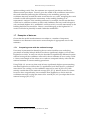
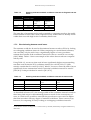
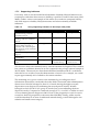
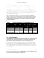
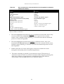
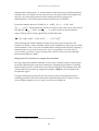
Synthetic estimation of healthy
lifestyles indicators: User guide
Shaun Scholes, Madhavi Bajekal, Kevin Pickering
Synthetic estimation of healthy
lifestyles indicators: User guide
Shaun Scholes, Madhavi Bajekal, Kevin Pickering
Prepared for the Department of Health
January 2005
Contents
EXECUTIVE SUMMARY .........................................................................................1
1
BACKGROUND AND GUIDANCE ON USE .............................................3
1.1
1.2
1.3
1.4
1.5
Introduction ...................................................................................................... 3
Estimation for small areas............................................................................... 3
Healthy lifestyle behaviours........................................................................... 3
Generating synthetic estimates (a model-based approach) ....................... 4
Limitations of the estimates............................................................................ 5
1.5.1
1.5.2
1.5.3
1.5.4
1.5.5
1.6
1.7
Banding/ranking of estimates ....................................................................... 7
Examples of data use ....................................................................................... 8
1.7.1
1.7.2
1.7.3
2
Comparing areas with the national average ............................................8
Discriminating between small areas .........................................................9
Supporting indicators................................................................................10
ESTIMATES ......................................................................................................11
2.1
The healthy lifestyle indicators .................................................................... 11
2.1.1
2.1.2
2.1.3
2.1.4
2.1.5
2.2
2.3
3
Synthetic estimates and performance monitoring...................................5
Confidence intervals....................................................................................6
Geographical boundaries............................................................................7
Timeliness .....................................................................................................7
Estimates for subgroups within small areas ............................................7
Current smoking ........................................................................................11
Obesity.........................................................................................................11
Fruit and vegetable consumption (children)..........................................11
Fruit and vegetable consumption (adults) .............................................12
Binge drinking............................................................................................12
Confidence intervals...................................................................................... 12
Data files.......................................................................................................... 13
GUIDE TO THE METHODOLOGY.............................................................14
3.1
Datasets used .................................................................................................. 14
3.1.1
3.1.2
3.2
3.3
3.4
The survey dataset .....................................................................................14
The covariate dataset.................................................................................15
Deriving the ward estimates ........................................................................ 16
Deriving the PCO estimates ......................................................................... 17
Validating the models ................................................................................... 17
REFERENCES ...........................................................................................................19
APPENDIX A
AREA CHARACTERISTICS ASSOCIATED WITH THE HEALTHY
LIFESTYLE MEASURES ......................................................................................20
APPENDIX B
PRODUCING SYNTHETIC ESTIMATES (A WORKED EXAMPLE)............24
National Centre for Social Research
EXECUTIVE SUMMARY
•
The National Centre for Social Research (NatCen) was commissioned by the
Department of Health to produce estimates of healthy lifestyle behaviours using
Health Survey for England (HSfE) data.
•
The aim of the project was to respond to the twin requirements of developing
small area estimates for publication on the Neighbourhood Statistics (NeSS)
website and of providing key public health information not currently available
from any other source.
•
Estimates and 95% confidence intervals, covering the period 2000 to 2002, have
been produced for wards and Primary Care Organisations (PCOs). The health
behaviours covered are current smoking, obesity and binge drinking for adults,
and fruit and vegetable consumption for children and adults separately.
•
Confidence intervals were produced in order to make the margin of error around
the estimates clear. We recommend that users view the prevalence for a ward or
PCO in light of its confidence interval.
•
Statistical modelling was used to produce the estimates because the sample size
of national surveys is too small at ward-level to provide reliable estimates.
•
These model-based estimates are of a different nature from standard survey
estimates. They must be used with caution. The models estimate the expected
prevalence of health behaviours for any ward or PCO given the social and
demographic characteristics of its population. They are not therefore estimates
of the actual prevalence for wards or PCOs.
•
The large confidence interval around the estimates meant that wards could not
be ranked within PCOs, or Strategic Health Authorities (SHAs), or nationally –
the margin of error around such rankings would render such an exercise to be
meaningless.
•
It is important that users note that the estimates do not take account of any
additional local factors that may impact on the true prevalence rate. The
estimates, therefore, cannot be used to monitor performance or change over
time.
•
The methodology used does not enable separate estimates for specific population
sub-groups to be produced within each ward or PCO.
•
The estimates could be used in a number of appropriate ways. For example, the
data could be used to identify those wards or PCOs which had an expected
prevalence of health behaviours that was significantly higher or lower than
England as a whole. Wards having an expected prevalence that was significantly
higher or lower than the model-based estimate for their PCO could also be
identified.
1
National Centre for Social Research
•
The large width of the confidence intervals attached to the ward-level estimates
means that it would not be possible to state that the expected prevalence in one
ward was higher than that in another with any degree of statistical confidence.
There is more scope, however, for using the estimates to discriminate between
PCOs.
•
The methodology adopted for this project was used previously by the Office for
National Statistics (ONS) to produce ward-level income estimates and has been
extensively reviewed by academics with expert knowledge of small area
estimation. A range of checks were used to ensure that the assumptions made by
the models were valid. The published estimates have also been validated against
other health behaviour data sources including the 2003 HSfE.
2
National Centre for Social Research
1 BACKGROUND AND GUIDANCE ON USE
1.1 Introduction
This document provides a guide to how the synthetic estimates of healthy lifestyle
behaviours should be used and the way in which the estimates have been developed.
This first chapter of the report provides the background to the project and guidance
on the use of the estimates. The second chapter describes the estimates produced by
the project. The last chapter provides a non-technical overview of the methodology
used to produce the estimates.
1.2 Estimation for small areas
The basic problem with national surveys such as the Health Survey for England
(HSfE) is that they are not designed for efficient estimation for small areas such as
electoral wards (Heady et al., 2003).
First, prevalence estimates of health behaviours such as current smoking based on
the sample data can only be computed for a subset of all wards (i.e. those wards
containing respondents to the survey). The adult respondents to the 2000 to 2002
health surveys, for example, belonged to only 40% of the wards in England.
Second, for those wards containing survey respondents, the achieved sample size
will usually be small and the estimates will thus have low precision. This low
precision will be reflected in rather wide confidence intervals for the survey
estimates. Other more complex techniques are therefore needed to generate precise
ward-level estimates.
‘Synthetic estimation’ describes the several different ways in which more precise
ward-level estimates might be constructed. The key idea is that to produce
prevalence estimates of healthy lifestyle behaviours such as current smoking for a
particular ward with an adequate level of precision it is necessary to use a technique
that takes advantage of information on smoking from wards other than itself. This
information is brought into the estimation process through a statistical model.
1.3 Healthy lifestyle behaviours
The National Centre for Social Research (NatCen) was commissioned by the
Department of Health to produce ward-level estimates of five healthy lifestyle
behaviours using HSfE data. The project involved three main stages:
3
National Centre for Social Research
•
•
•
scoping and feasibility – review of existing approaches to synthetic estimation
to assess the various options and identification of the data requirements
(Stage 1:Bajekal et al., 2004);
testing and validation: of selected alternate methods of synthetic estimation
(Stage 2:Pickering et al., 2004); and
implementation – producing small area estimates based on a best method
identified in stage 2 for five health behaviours and accompanying reports,
spreadsheets, metadata and user guidance for publication on the
Neighbourhood Statistics (NeSS) website and dissemination to the health
community (Stage 3:Pickering et al., 2005)1.
Model-based estimates with 95% confidence intervals have been produced for five
healthy lifestyle behaviours covering the period 2000 to 2002. The estimates have
been produced at two levels: Census Area Statistics (CAS) ward and Primary Care
Organisation (PCO). The five healthy lifestyle behaviours covered are:
•
•
•
•
•
current smoking for adults (aged 16 years or more);
obesity for adults (aged 16 years or more);
binge drinking for adults (aged 16 years or more);
consumption of five or more portions of fruit and vegetables per day for
adults (aged 16 years or more); and
consumption of three or more portions of fruit and vegetables per day for
children (aged from 5 to 15 years inclusive).
The aim of the project was to respond to the twin requirements of developing small
area estimates for NeSS and of providing key public health information not currently
available from any other source. In particular, we expect the estimates to assist
Primary Care Organisations to identify wards within their area with high levels of
unhealthy behaviours and to plan local services accordingly.
1.4 Generating synthetic estimates (a model-based approach)
A model-based approach to produce estimates of healthy lifestyle behaviours was
used because the sample size of national surveys is too small at ward-level to
provide reliable estimates. Most national surveys are designed to provide a large
enough sample to calculate national or regional estimates. To ensure that the national
sample is representative of different types of people and areas in the country, a
relatively small number of areas are selected at random from across the country. As a
result, many small areas such as electoral wards either contain no respondents as
they were not covered by the survey, or too few respondents to calculate reliable
estimates.
The model-based method used to produce the ward-level estimates combined two
sets of information. First, the HSfE provided health behaviour data (e.g. whether a
respondent currently smoked or not). Second, the 2001 Census and other
1
Reports can be found on the NatCen website (www.natcen.ac.uk), along with a project summary.
4
National Centre for Social Research
administrative data sources provided information about the characteristics of the
area in which respondents lived. A statistical model was used to examine the
relationships between the healthy lifestyle behaviours and area characteristics. As
part of the modelling process, for example, we examined whether the propensity for
a person to be a current smoker varied significantly between regions or between
wards with varying proportions of residents who were living as a couple, claiming
Income Support, had a limiting longstanding illness etc. The final model was then
used to calculate the prevalence estimate of current smoking for all wards and PCOs
in England.
The model-based approach generates estimates that are of a different nature from
standard survey estimates because they are dependent upon how well the
relationship between healthy lifestyle behaviours for individuals and the
Census/administrative information about the area in which they live is specified.
Section 3 of this User Guide provides a brief non-technical overview of the
methodology used. For a fuller technical description of the methodology users are
referred to the Stage 3 report (Pickering et al., 2005).
1.5 Limitations of the estimates
The estimates resulting from this project must be used with caution. Synthetic
estimates are difficult to interpret because they are model-based. Although robust,
they will almost certainly not mirror precisely any available measures from local
studies or surveys (although research by NatCen and others have shown that they
tend to be related). In this section we discuss a number of limitations that users must
bear in mind when using the data.
1.5.1
Synthetic estimates and performance monitoring
Ward or PCO level estimates based exclusively on sample respondents located
within the area itself are easy to interpret. They represent an estimate of the real
prevalence of health behaviours such as current smoking for the area in question.
Synthetic estimates, however, are more difficult to interpret. This is because the
synthetic estimate for a particular ward is a model-based estimate, and the model
that we use estimates the underlying expected value of smoking prevalence for any
ward given the social and demographic characteristics of its population. They are
not therefore estimates of the actual prevalence for wards or PCOs. To interpret the
estimates it is recommended that users adopt statements such as: given the
characteristics of the local population we would expect approximately x% of adults within
ward X to smoke/be obese etc (Health Development Agency, 2004).
As the synthetic estimates do not measure actual prevalence within small areas we
do not encourage any ranking of wards within their PCO or Strategic Health
Authority (SHA). (The large margin of error around any such ranking would also
render such an exercise to be meaningless - for more details on ranking see Section
1.6.)
5
National Centre for Social Research
It is important that users note that the estimates do not take account of any
additional local factors that may impact on the true prevalence rate (e.g. local
initiatives designed to reduce smoking, obesity or binge drinking). The estimates,
therefore, cannot be used to monitor performance or change over time.
1.5.2
Confidence intervals
NatCen has produced confidence intervals to accompany the model-based estimates
in order to make the margin of error around the estimates clear. The interval reflects
the range between which the true value is believed to lie, at a given level of
confidence. The confidence intervals therefore represent the uncertainty in the
modelling process. At the 95% confidence level, assuming that the model is a good
representation of reality, the confidence interval is expected to contain the true value
around 95 times out of 100. For example, if a ward estimate of current smoking is
49% and the 95% confidence interval is [32%,67%] we know that 95% of the time the
true prevalence estimate for that ward (based on its local population characteristics)
will fall within this range.
It is important to take into account the margin of error around the estimates when
interpreting them. We therefore recommend that rather than focus exclusively on the
prevalence estimate, users view the prevalence for a ward or PCO in light of its
confidence interval.
The average width of the confidence intervals, both for wards and PCOs, varied
across the five healthy lifestyle behaviours. Table 1.1 shows that the confidence
intervals are widest for children’s fruit and vegetable consumption and smallest for
obesity (for more details on the factors influencing the width of the confidence
intervals see Pickering et al., 2005).
Table 1.1
Average width of the 95% confidence intervals for the 5 healthy
lifestyle behaviours (wards and PCOs)
Health behaviour
Average width of the 95%
confidence interval
Wards
PCOs
± 11%
± 7%
± 12%
± 13%
± 19%
Current smoking 2
Obesity
Binge drinking
Fruit and vegetable consumption (adults)
Fruit and vegetable consumption (children)
± 3%
± 2%
± 3%
± 3%
± 5%
The width of the confidence intervals, particularly at ward-level, represent a further
limitation on using the estimates. As will be discussed in Section 1.7.2 one potential
use of the estimates is to discriminate between wards or PCOs by looking at
2
For a ward whose prevalence estimate of current smoking was 30%, a confidence interval of width
± 11% would correspond to a range of 19% to 41%. Similarly, for a PCO whose estimate was 30%, a
confidence interval of width ± 3% would correspond to a range of 27% to 33%.
6
National Centre for Social Research
overlapping confidence intervals. When comparing two model-based estimates, one
ward may only be said to have a significantly higher or lower prevalence estimate
than another if the confidence intervals for the two wards do not overlap.
The average width of the confidence intervals implies, however, that there would be
little scope for discriminating between wards. As an extreme example, in the case of
current smoking, only 16 of the 7,958 wards were significantly different from the
ward having the ‘average’ estimate. Therefore, it is very important that the wardlevel estimates are used with great caution by users; in the vast majority of cases, it
would not be possible to state that the prevalence in one ward was higher than that
in another with any degree of statistical confidence.
1.5.3
Geographical boundaries
The ward estimates have been produced on 2003 Census Area Statistics (CAS) ward
boundaries (the standard set of boundaries used for Neighbourhood Statistics) and
therefore cannot be translated onto any other boundary system. Users must be aware
of this when using the estimates in any application or drawing conclusions from the
data. It is inadvisable, for example, to aggregate the ward estimates to compute a
Local Authority District estimate in the absence of any published confidence
intervals for that higher level of geography.
1.5.4
Timeliness
We stress that recombining estimates to new boundaries as they change over time
will not be feasible. The estimates are also based on specific years of survey data
(2000 to 2002 for smoking, obesity and binge drinking, and 2001 to 2002 for fruit and
vegetable consumption) and so are only valid for these time periods.
1.5.5
Estimates for subgroups within small areas
The methodology used to produce the estimates does not support the production of
separate estimates for specific population sub-groups within each ward or PCO. For
example, the estimate of current smoking prevalence represents the underlying
expected value for the demographic and social mix of adults (aged 16 years or more)
living in a ward at the time of the 2001 Census. It cannot, therefore, tell us what
proportions of those living in the ward smoke by age, sex or social class.
1.6 Banding/ranking of estimates
NatCen have made no attempt to rank the wards or assign them to bands (e.g. the
highest 10% of wards, middle 80% and lowest 10%). There are two arguments
7
National Centre for Social Research
against ranking wards. First, the estimates are expected prevalences and do not
measure actual prevalence. Second, given the width of the confidence intervals for
the ward estimates (reflecting the uncertainty in the modelling process), the
confidence intervals around the ranks would also be very wide. Assigning the wards
to bands would still require the uncertainty in the ranking/banding to be
represented3. Analysis of the smoking estimates, for example, has shown that there
would not be sufficient evidence to state with confidence that any ward belonged to
only one band (highest 10%, middle 80% and lowest 10%) once the uncertainty in the
banding had been accounted for. Hence, a ward belonging to the highest 10% of
wards could also be plausibly located within the middle 80%.
1.7 Examples of data use
Given that the model-based estimates are subject to a number of important
limitations we illustrate in this section some examples of appropriate uses for the
estimates.
1.7.1
Comparing areas with the national average
Users may be interested in identifying those wards which have an underlying
prevalence of healthy lifestyle behaviours that is significantly higher or lower than
England as a whole. A ward can only be described as significantly different from the
national average if the confidence intervals for those estimates do not overlap. Table
1.2 shows an example of this where two wards are compared side-by-side with the
national estimate of current smoking prevalence.
Using Table 1.2, we can say that ward A has a significantly higher current smoking
rate than England as a whole at the 5% significance level since the 95% confidence
intervals do not overlap (i.e. the confidence interval for ward A [32%,67%] falls
entirely outside that for the national average [25%,27%]). Ward B, however, cannot
be said to have a significantly lower estimate than England as a whole since the
confidence intervals overlap (the interval for ward B [9%,30%] overlaps that for the
national average [25%,27%]).
3
For a technical discussion of ranking see Bird et al., 2003.
8
National Centre for Social Research
Table 1.2
England4
Ward A
Ward B
Smoking estimates and 95% confidence intervals for England and two
wards
95% confidence intervals for percentage who
currently smoke
Estimate
Lower
Upper
confidence
confidence
limit
limit
26%
25%
27%
49%
32%
67%
17%
9%
30%
The same line of reasoning can be easily extended to comparing wards to the modelbased estimate for their PCO. Such comparisons may enable PCOs to identify wards
within their area with high levels of unhealthy behaviours.
1.7.2
Discriminating between small areas
The estimates could also be used to discriminate between wards or PCOs by looking
at overlapping confidence intervals. When comparing two model-based estimates,
one ward may only be said to have a significantly higher or lower prevalence
estimate than another if the confidence intervals for the two wards do not overlap
(ONS, 2004a). Table 1.3 shows an example of this where three wards are compared
side-by-side.
Using Table 1.3, we can say that ward A has a significantly higher current smoking
rate than ward B since the 95% confidence interval for ward A [32%,67%] falls
entirely outside that for ward B [9%,30%]. Ward C, however, cannot be said to have a
significantly lower estimate than ward A since the confidence interval for ward C
[34%,54%] overlaps with that for ward A [32%,67%].
Table 1.3
Ward A
Ward B
Ward C
Smoking estimates and 95% confidence intervals for three wards
95% confidence intervals for percentage who currently smoke
Estimate
Lower confidence
Upper confidence
limit
limit
49%
32%
67%
17%
9%
30%
42%
34%
54%
As described in Section 1.5.2, the average width of the confidence intervals results in
there being little scope for discriminating between wards. In the vast majority of
cases, it would not be possible to state that the prevalence in one ward was higher
than that in another with any degree of statistical confidence. There is more scope,
however, for comparing PCOs by looking at overlapping confidence intervals.
Note that the estimate for England is a standard survey estimate, obtained by using the health survey
data alone.
4
9
National Centre for Social Research
1.7.3
Supporting indicators
Users may wish to use the model-based estimates of healthy lifestyle behaviours in
conjunction with other data sources to build up a profile of wards in their area (ONS,
2004a). Table 1.4 shows an example of this where two wards are compared side-byside with respect to healthy lifestyle measures and other externally available
indicators.
Table 1.4
Using supporting indicators to build up a ward profile
Indicator
Survey-based estimate of
current smoking, with 95%
confidence interval
Model-based estimate of current
smoking, with 95% confidence
interval
Index of Multiple Deprivation
ranking (2004): 10 bands of
equal size with 1 indicating the
least deprived wards and 10 the
most deprived
% Adults claiming Income
Support
% properties in council tax band
H (£320,000+)
Urban/rural classification of
wards
England
26% [25%,27%]
Ward A
Not applicable
Ward B
Not applicable
Not applicable
49% [32%,67% ]
17% [8%,30%]
Not applicable
10
3
5.2%
22.0%
2%
0.6%
0
0.8%
Not applicable
Traditional
manufacturing
Suburbs and
Small Towns
The first row shows the standard survey national estimate for England. This estimate
has a narrow confidence interval as it was computed using a large national sample of
30,872 adults. The second row lists the model-based estimates and 95% confidence
intervals for two wards. Given the characteristics of ward A, for example, we would
expect approximately 49% of adults to be current smokers.
The remaining rows give a context to the estimates by providing area-level
information about these wards taken from the 2001 Census and other administrative
data sources. Ward A belonged to the 10% of wards having the highest overall
deprivation score (high scores indicating the most deprived wards). Ward B
belonged to the lower 20%-30% group of wards (low scores indicating the least
deprived wards). Compared to a national average of 5%, over 20% of adults in ward
A were claiming Income Support in 2001. None of the properties in ward A were in
council tax band H (properties worth more than £320,000). Finally, whilst ward A
could be described as an area of traditional manufacturing, ward B belonged to the
suburbs and small towns category.
10
National Centre for Social Research
2 ESTIMATES
This chapter describes the estimates produced by the project. It is important that
users note that the methodology used to produce the five sets of estimates is
relatively new and as a result may be subject to consultation, modification and
further development. In view of this ongoing work these estimates are being
published as experimental statistics.
2.1 The healthy lifestyle indicators
The five sets of estimates published by the project are for current smoking, obesity,
and binge drinking for adults, and fruit and vegetable consumption for children and
adults separately. In this section we provide more details on the derivation of these
healthy lifestyle indicators using the Health Survey for England.
2.1.1
Current smoking
The healthy lifestyle indicator for current smoking was generated from the HSfE
measure of “current smoking status”. Adult respondents (aged 16 years or more) to
the HSfE were defined to be current smokers if they reported that they were a
“current cigarette smoker”, and not a current smoker if they reported that they had
“never smoked cigarettes at all”, “used to smoke cigarettes occasionally” or “used to
smoke cigarettes regularly”. Of the 30,872 adults from the combined HSfEs from 2000
to 2002, 7,972 (26%) reported that they were current smokers.
2.1.2
Obesity
The healthy lifestyle indicator for obesity was generated from the height and weight
of adult respondents (aged 16 years or more), as measured by the HSfE interviewers.
The Body Mass Index (BMI) was derived from the height and weight as: the weight
in kilograms divided by the square of the height in meters. Respondents were
defined to be obese if their BMI measure was more than 30. Of the 27,120 adults from
the combined HSfEs from 2000 to 2002, 5,991 (22%) were obese.
2.1.3
Fruit and vegetable consumption (children)
The healthy lifestyle indicator for fruit and vegetable consumption for children (aged
from 5 to 15 years inclusive) was generated from the data collected in the HSfE about
the quantities of different types of fruit and vegetable consumed on the previous
day. These measures were combined to give the total number of portions of fruit and
vegetable consumed.
11
National Centre for Social Research
Note that information about fruit or vegetable consumption was not collected in the
HSfE 2000, nor for children under 5 years old in the HSfE 2001 and 2002. Of the 8,438
children (aged 5 to 15 years) in the 2001 and 2002 HSfEs, 3,163 (37%) had consumed
three or more portions of fruit and vegetables. The healthy lifestyle measure was
whether the child had consumed three or more portions or not5.
2.1.4
Fruit and vegetable consumption (adults)
The healthy lifestyle measure for fruit and vegetable consumption for adults (aged 16
years or more) was generated from the data collected in the 2001 and 2002 HSfEs
about the quantities of different types of fruit and vegetable consumed on the
previous day. These measures were combined to give the total number of portions of
fruit and vegetable consumed. Of the 23,039 adults in the 2001 and 2002 HSfEs, 5,460
(24%) had consumed five or more portions of fruit and vegetables. The healthy
lifestyle measure was whether an adult respondent had consumed five or more
portions or not.
2.1.5
Binge drinking
The healthy lifestyle measure for binge drinking was generated from the data
collected in the HSfE about the quantities of all the different types of alcoholic drinks
(beer, wine, spirits, sherry and alcopops) consumed on a respondent’s heaviest
drinking night in the previous week. These measures were combined to give the
number of units of alcohol consumed on the heaviest drinking day. Binge drinking
was then defined separately for men and women: men were defined as having
indulged in binge drinking if they had consumed 8 or more units of alcohol on the
heaviest drinking day in the previous seven days; for women the cut-off was 6 or
more units of alcohol. Of the 30,440 adults in the 2000 to 2002 HSfEs, 5,539 (18%)
were defined to have indulged in binge drinking.
2.2 Confidence intervals
The five sets of estimates have been produced for 7,958 Census Area Statistics wards
and 303 PCOs (as at 2003) in England6. As well as producing estimates it is also
important to be able to assess the accuracy of the estimates. We do this by placing
confidence intervals around the estimates. As the true prevalence is unknown, a
range is produced (i.e. a ‘confidence interval’) within which we are fairly certain that
the true value lies. On average we would expect the confidence interval to contain
the true population value 95% of the time.
Note that the measure of three or more portions was used rather than the target figure of five or more
because the proportion of children in the HSfE eating five or more portions was only 12%. It was felt
that this was too low a prevalence to obtain reliable synthetic estimates.
5
Census Area Statistics (CAS) wards are used for 2001 Census outputs, including those available on the
NeSS website. They are identical to the 2003 Statistical Wards except that 18 of the smallest wards have
been merged into other wards to avoid the confidentiality risks of releasing data for very small areas.
This has occurred to those wards with fewer than 100 residents or 40 households (as at the 2001
Census). There are a total of 7,969 CAS wards in England. For the purposes of this project we have
combined together the nine wards in the City of London and four in the Isles of Scilly into one unit
respectively to form 7,958 CAS wards. This classification of wards mirrors that used by the Department
of Work and Pensions for publishing ward-level claimant counts.
6
12
National Centre for Social Research
Complex methods were used to derive confidence intervals for the synthetic
estimates. For a fuller technical description of the methodology users are referred to
the Stage 3 report (Pickering et al., 2005).
2.3 Data files
Separate excel workbooks have been produced for each healthy lifestyle measure:
each workbook containing a separate sheet for wards and PCOs. The survey-based
national estimate for England, and its accompanying confidence interval, is provided
at the top of the sheet for reference. The variable names and labels in each worksheet
are shown in Table 2.1.
Table 2.1
Column name
GORcode
GORname
SHAcode
SHAname
PCOcode
PCOname
WARDcode
WARDname
Estimate
Lower
Upper
Variable names and labels in the data files
Column label
Government Office Region code
Government Office Region name
Strategic Health Authority code
Strategic Health Authority name
Primary Care Organisation code
Primary Care Organisation name
CAS ward code (not in PCO sheet)
CAS ward name (not in PCO sheet)
Model-based estimate of prevalence
Lower 95% confidence interval limit
Upper 95% confidence interval limit
In accordance with the Guidance for the Presentation of Government Statistics for
Health Areas (ONS, 2004b) the ward estimates are presented in the following nested
order: wards within reporting PCO, within SHA, within GOR. Wards are listed in
CAS ward code order and PCOs and SHAs in alphabetical order within GORs. These
tables are published on the accompanying electronic files on the NeSS website.
13
National Centre for Social Research
3 GUIDE TO THE METHODOLOGY
This chapter provides a brief non-technical description of the methodology used for
producing model-based estimates of healthy lifestyle behaviours for all wards and
PCOs in England. A full description of the methodology can be found in the
Synthetic Estimation of Healthy Lifestyles Indicators Stage 3 report (Pickering et al.,
2005).
3.1 Datasets used
3.1.1
The survey dataset
The Health Survey for England (HSfE) comprises a series of annual surveys. All
surveys have covered the adult population aged 16 and over living in private
households in England. The HSfE series is part of an overall programme of surveys
commissioned by the Department of Health and designed to provide regular
information on various aspects of the nation’s health. Each survey in the series
consists of core questions and measurements (for example, anthropometric and
blood pressure measurements and analysis of blood and saliva samples) which are
included each year, plus modules of questions on specific health conditions that are
repeated at regular intervals. Questions relating to smoking and drinking have
appeared in each year of the survey (1994 to 2003). Height and weight measurements
have also been taken each year. A new module of questions relating to fruit and
vegetable consumption was introduced in 2001 and has appeared every year since.
For the purposes of this study three years of HSfE data (2000, 2001 and 2002) were
merged together to form a combined survey dataset of health behaviour data. The
reasons for selecting these particular years were that they included the most up-todate HSfE information available and that the years were symmetrically arranged
either side of 2001, the year the last Census was carried out.
Each year the HSfE covers a representative sample of people resident in households,
and in addition, in certain years particular population groups are over-sampled or
“boosted”. In 2000, a separate sample of older people (aged 65 and over) resident in
care homes was included. In 2002, a separate sample of infants and children (aged 015), young adults (aged 16-24) and mothers with infants aged less than 1 was
undertaken.
Typically the annual sample size of the general population is about 16,000 adults
aged 16 and over and 4,000 children aged 0-15. In years when special populations are
boosted, the general population sample is halved to about 8,000, as was the case in
2000 and 2002. Only the general population samples in each year were used for the
adult health behaviour measures. The boost sample of children in 2002 was included,
however, for children’s fruit and vegetable consumption.
14
National Centre for Social Research
The HSfE data were supplied at the individual level with the postcode of the
respondent attached. The February 2004 release of the All Fields Postcode Directory
was used to allocate these postcodes to 2003 Census Area Statistics (CAS) ward
boundaries, Local Authority Districts and Government Office Region.
Although CAS wards (the principal estimation area chosen for this project) nest
within higher-level administrative tiers such as Local Authority Districts and
Government Office Regions they do not nest perfectly into larger health areas such as
PCOs. NatCen was provided a ‘best-fit’ one-to-one look-up table to uniquely
attribute whole wards to a PCO7.
Table 3.1 summarises the number of survey observations used to calculate the
estimates. In the case of current smoking, for example, 30,872 adult respondents to
the 2000 to 2002 health surveys covered 3,231 of the 7,958 CAS wards in England.
The average number of respondents per ward was 10, although 225 wards only
contained 1 respondent.
Table 3.1
Descriptive statistics for the surveyed HSfE wards and PCOs
Health behaviour
measure
Number of
HSfE
respondents
Number of
wards
covered
Current smoking
Obesity
Binge drinking
Fruit and vegetable
consumption (adults)
Fruit and vegetable
consumption (children)
30,872
27,120
30,440
23,039
8,438
3.1.2
3,231
3,149
3,230
2,644
Number of
wards
containing
only 1
respondent
225
244
230
211
Average
number of
respondents
per ward
and PCO
10 (102)
9 (90)
9 (101)
9 (76)
Maximum
number in
any sampled
ward
60
56
60
60
1,989
400
4 (28)
28
The covariate dataset
The term ‘covariate’ describes those area-level characteristics (e.g. deprivation scores,
life expectancy rates, rural/non-rural indicator, Government Office Region) that
were potentially related to health behaviours such as smoking and obesity.
Because of its universal geographical and population coverage, the 2001 Census
provided the main source for demographic and social covariate data. The full set of
Census and administrative datasets that were merged together to provide the arealevel characteristics that were considered for inclusion in the statistical models are
shown in Table 3.2.
The lack of an exact fit between wards and PCOs introduces a further source of error when calculating
the confidence intervals for the PCO estimates. At present the ONS is carrying out work on this
problem. The results of this research, however, will not be available until later in the year. As yet,
therefore, NatCen has been unable to take account of this additional error – meaning that the margin of
error around the PCO estimates may be slightly underestimated.
7
15
National Centre for Social Research
Table 3.2
Area-level characteristics considered for inclusion in the statistical
models of healthy lifestyles
Area-level characteristics
Local Authority District level
Mortality rates
Deprivation scores (ID 2004)
Ward level
Key Statistics & Standard Tables
All-cause Standardised Mortality Ratios
Area-type classification
Deprivation scores8 (ID 2004 derived)
Claimant counts
Rural/non-rural indicator
Proportionate distribution of properties in
the council tax bands (A-X)
Source
Compendium of Clinical and Outcome Indicators, 2003
Office of the Deputy Prime Minister, 2004
Census, 2001
Office for National Statistics
Office for National Statistics,2004
Office of the Deputy Prime Minister, 2004
Department of Work and Pensions, 2001
Department of the Environment, Food and Rural
Affairs, 2004
Valuation Office Agency, 2001
3.2 Deriving the ward estimates
The process of generating model-based estimates of healthy lifestyle behaviours
involved two main stages:
•
using a statistical model to represent as well as possible the relationships
between health behaviours and area-level characteristics; and
•
applying that model to calculate prevalence estimates for all wards in
England.
In the case of smoking, the first-stage involved finding the best model to describe the
relationship between whether an adult respondent to the HSfE currently smoked or
not and the characteristics of the area in which the person lived.
Different area-level characteristics were associated with different health behaviours.
The results from the modelling procedures are presented for each health behaviour
in Appendix A.
The second stage involved applying the results from the model to calculate
prevalence estimates, using the Census/administrative information available for all
wards. A detailed worked example of how model-based estimates can be produced
in practice is outlined in Appendix B9.
The deprivation scores were aggregated to ward level using a weighted average of the deprivation
scores produced for lower level Census Super Output Areas.
9 The material provided in Appendices A and B is more technical and hence users should consider them
as optional.
8
16
National Centre for Social Research
Complex methods were used to derive confidence intervals for the synthetic
estimates. For a fuller technical description of the methodology users are referred to
the Stage 3 report (Pickering et al., 2005).
3.3 Deriving the PCO estimates
Synthetic estimates for 303 Primary Care Organisations in England were calculated
by aggregating the model-based estimates for the component wards, weighting the
contribution of each ward in proportion to its population size, derived from the
Census 2001 counts10. The corresponding confidence intervals for the PCO estimates
were generated using a similar method as for wards (see Pickering et al., 2005).
3.4 Validating the models
The methodology used for this project was used previously by the Office for
National Statistics to produce ward-level income estimates (Longhurst et al., 2004)
and has been extensively reviewed by academics with expert knowledge of small
area estimation. A range of checks were used to assess the appropriateness of the five
models and to examine whether the models were correctly specified. The results of
the tests showed that the models were indeed well specified and that the
assumptions made were valid. This provided confidence in the accuracy of the
estimates and the confidence intervals attached to them.
Having generated the estimates, a two-stage validation process was undertaken to
establish the plausibility of the estimates. The first stage involved external validation
of the estimates by comparison with other health behaviour data sources. These data
sources were:
•
•
•
•
•
Camden and Islington Health Authority Survey, 1999;
National Patient Survey in Primary Care Organisations, 2003;
Wigan, Bolton and Bury Health Authority Surveys, 2001;
Liverpool, Sefton, St Helens and Knowsley Lifestyle Surveys, 2001; and
Health Survey for England, 2003.
The model-based estimates were compared with these data sources both by actual
value and by rank. Statistical measures of association were also computed to assess
the relationship between the model-based estimates and those available via the
external data sources (see Pickering et al., 2005).
The second stage was a consultation exercise that involved local users, academics
and health related experts as members of project management committees. This
consultation enabled NatCen to invite users to comment upon the plausibility and
10 The adult population counts were used for the adult health behaviours, and the 5-15 year old counts
were used for children’s fruit and vegetable consumption.
17
National Centre for Social Research
usefulness of the estimates. The comments received informed the approach we have
used and generally supported the plausibility of the estimates.
18
National Centre for Social Research
REFERENCES
Bajekal M, Scholes S, Pickering K and Purdon S (2004) Synthetic estimation of healthy
lifestyle indicators: Stage 1 report. (http://www.natcen.ac.uk)
Bird S, Cox D, Farewell V, Goldstein H, Holt T and Smith P (2003) Performance
Indicators: Good, Bad and Ugly. Royal Statistical Society Working Paper on
Performance Monitoring in the Public Service.
Goldstein H (2003) Multilevel Statistical Models. London, Arnold.
Heady P, Clarke P and others (2003) Model-based small area estimation series No 2 Small
Area Estimation Project Report, ONS.
Health Development Agency (2004) The Smoking Epidemic in England.
Longhurst J, Cruddas M, Goldring S and Mitchell B (2004) Model-Based Estimates of
Income for Wards, 1998/99 Technical Report. ONS.
ONS (2004a) Model-Based Estimates of Income for Wards in England and Wales, 1998/99
User Guide
(http://neighbourhood.statistics.gov.uk/information/income_estimates.pdf)
ONS (2004b) Guidance for the Presentation of Government Statistics for Health Areas at
Regional, Health Authority/Health Board and Primary Care Levels.
(http://www.statistics.gov.uk/geography/health_areas.asp)
Pickering K, Scholes S and Bajekal M (2004) Synthetic estimation of healthy lifestyle
indicators: Stage 2 report. (http://www.natcen.ac.uk)
Pickering K, Scholes S and Bajekal M (2005) Synthetic estimation of healthy lifestyle
indicators: Stage 3 report. (http://www.natcen.ac.uk)
Twigg L, Moon G and Jones K (2000) Predicting small-area health-related behaviour:
a comparison of smoking and drinking indicators Social Science and Medicine 50(7-8):
1109-20.
19
National Centre for Social Research
APPENDIX A AREA CHARACTERISTICS ASSOCIATED WITH THE
HEALTHY LIFESTYLE MEASURES
The model-based approach we have used to calculate the ward-level estimates was
based on finding a relationship between individual health behaviour measures and
Census/administrative information about the areas in which people lived. This
relationship, expressed in a statistical model, was then used to calculate the
prevalence estimates for all wards in England. The ward-level estimates were then
used to calculate estimates for all PCOs.
In this section we present the five optimal models of healthy lifestyles used to
calculate the estimates. Note that each item was retained in the model because it had
a significant association with the health behaviour measure (allowing for the other
area characteristics in the model), not because we considered there to be a direct
relationship between them. Hence the models should not be interpreted by users as
explanatory models of health behaviour.
Tables A.1 and A.2 show the significant area characteristics associated with the
health behaviours. (The definitions of the area characteristics are shown in Tables A.3
to A.6.) In the case of smoking, for example, being located in the North West region
was associated with increased propensity for a person to be a current smoker. In
contrast, being located in the South West region was associated with decreased
propensity for a person to smoke (for more details see Pickering et al., 2005).
Table A.1
Area characteristics associated with smoking, obesity and binge
drinking
Current smoking
Proportion female, aged 25-34
illsiwrk
3rd most deprived band of
wards (imd8) 11
North West region
eduscore
imd5
icouple
iethnic
iprofman
aarate
South West region
aarate * North West region
iethnic * South West region
imd8 * South West region
Obesity
iolevel
isroutin
South West region
Binge drinking
North East region
North West region
Yorks & The Humber region
laidscor
East of England region
propctxg
hloamnty
rural * isroutin
laidscor * East of England region
Proportion male, aged 45-49
icouple
iethnic
israte
Proportion male, aged 75-79
South West region
Proportion female, aged 50-54
Proportion female, aged 85+
hovercr
South East region
hovercr * South East region
aarate * South West region
11 Based on their deprivation score wards were grouped into one of 10 roughly equal sized bands,
where group 1 (imd1) represented the least deprived wards up to group 10 (imd10) indicating the most
deprived.
20
National Centre for Social Research
Table A.2
Area characteristics associated with fruit and vegetable consumption
(adults and children)
Fruit & vegetable consumption
(adults)
icobnuk
South East region
smr_10a
Yorks & The Humber region
2nd most deprived band of wards (imd9)
Built-up areas
Proportion female, aged 25-34
Proportion female, aged 16-19
smr_14b
isroutin
iupdcr50
smr_10a * South East region
isroutin * Yorks & The Humber region
Fruit & vegetable consumption
(children)
icobnuk
lemale
ipermsic
Yorks & The Humber region
West Midlands region
iolevel
empscore
iupdcr50
ipermsic * Yorks & The Humber region
empscore * South West region
icobnuk * London region
Notes to Tables A.1 and A.2:
•
The terms highlighted in bold had positive coefficients in the model: that is, they
were associated with an increased propensity for a person to be a current
smoker, obese, indulge in binge drinking, or consume more than the threshold
portions of fruit and vegetables.
•
The terms highlighted in italics had negative coefficients: that is, they were
associated with decreased propensity for a person to be a current smoker, obese,
indulge in binge drinking, or consume more than the threshold portions of fruit
and vegetables.
•
Within each batch of positive and negative terms the variables have been
arranged in decreasing order of statistical significance.
•
The terms containing an asterisk (*) are interaction terms. The majority of
interaction terms involved one of the Government Office Regions, meaning that
there was evidence to suggest that the ward characteristics had different
relationships with the health behaviour in different regions.
21
National Centre for Social Research
Definitions of the area characteristics in Tables A.1 and A.2
Table A.3
Variable
name
hloamnty
hovercr
icobnuk
icouple
iethnic
illsiall
illsiwrk
inoqual
iolevel
ipermsic
iprofman
isroutin
iupdcr50
Ward characteristics – Census 2001 data
Description
Proportion of households without central heating
Proportion of households overcrowded: occupancy
rating minus 1 or less
Proportion not born in UK, Ireland or European Union
Proportion 16+ residing as couple
Proportion non-white
Proportion with limiting longstanding illness
Proportion of working-age with limiting longstanding illness
Proportion 16-74 with no educational qualifications
Proportion 16-74 with highest qualification NVQ 1 or no qualifications
Proportion 16-74 permanently sick/disabled
Proportion 16-74 professional & managerial occupations (NS-SEC 1 & 2)12
Proportion 16-74 in semi-routine & routine occupations (NS-SEC 6 & 7)
Proportion unpaid carers caring > 50 hours per week
Table A.4
Variable name
aarate
dlarate
israte
propctxb
propctxg
12
Ward characteristics – Administrative data
Source
DWP benefits
data (Aug 2001)
“
“
Valuation
Office Agency
data (Mar 2001)
“
Description
Attendance allowance claimant rate
Disability living allowance claimant rate
Income Support claimant rate
Proportion of dwellings in council tax band B
Proportion of dwellings in council tax band G
National Statistics Socio-Economic Classification categories.
22
National Centre for Social Research
Table A.5
Variable name
Built-up areas
Other ward characteristics
imd8
Source
Classification of
wards, Office
for National
Statistics (2004)
Derived from
Output Area
scores produced
by the Office of
the Deputy
Prime Minister
(2004)
“
imd9
“
eduscore
“
Ward located in 3rd most deprived Index of Multiple
Deprivation (IMD) band
Ward located in 2nd most deprived Index of
Multiple Deprivation (IMD) band
Education, skills and training score
houscore
“
Barriers to housing and services score
imd5
Table A.6
Variable name
laidscor
lemale
smr_10a
smr_14b
Description
Ward located in 5th most deprived Index of Multiple
Deprivation (IMD) band
Local Authority District characteristics
Source
Office of the
Deputy Prime
Minister (2004)
Office for
National
Statistics
Compendium
of Clinical and
Outcome
Indicators
(2003)
“
Description
Index of Multiple Deprivation score
Life expectancy at birth, number of
years, 1999-2000
Mortality from stroke (icd10 i60-i69)
indirectly standardised ratios, 2001
Mortality from lung cancer (icd10 c33c34) indirectly standardised ratios
23
National Centre for Social Research
APPENDIX B PRODUCING SYNTHETIC ESTIMATES (A WORKED
EXAMPLE)
B.1
Modelling health behaviour data – a simple example
For health behaviour measures such as smoking (i.e. whether a person currently
smokes or not) a statistical model can be used to examine how characteristics such as
age, sex and social class influence the propensity of individuals to smoke.
We may be interested, for example, in using Health Survey for England data to
examine whether males are more likely to smoke than women. In this case, therefore,
current smoking status represents the ‘outcome’ variable about which comparisons
are made and sex denotes a factor which may have an influence on that outcome.
As current smoking status is a two-category (binary) outcome variable, a logistic
regression model is the natural one to use in order to examine if sex does influence
the propensity of individuals to smoke.
Using the combined 2000 to 2002 HSfEs we can specify a logistic regression model
where current smoking status is specified as the ‘outcome’ variable (1 = current
smoker, 0 = not a current smoker) and sex denoted as a factor (0 = female, 1 = male)
potentially related to smoking. The estimates from this model are shown in Table B.1.
Table B.1
A logistic regression model of current smoking using the combined
2000 to 2002 HSfEs
Variable
Odds ratio
95% confidence
interval for odds
ratio
Sex:
Females
Males
1.00
1.08
(baseline)
1.03 - 1.14
P-value
0.003
The estimates from the model give a measure of the effect of sex on current smoking
status. For ease of interpretation the estimates are presented as odds ratios. The
‘odds’ of an outcome is the ratio of the probability of its occurring to the probability
of its not occurring (e.g. if the probability of being a smoker is estimated to be 0.8
then the probability of not being a current smoker is 1.0-0.8 = 0.2 and so the odds of
being a smoker equal 0.8/0.2 = 4).
In this case, females are selected as the baseline or reference category, with males
being compared to them. There is no estimate, therefore, for females and the odds
ratio defined for males represents the ratio of the odds of being a current smoker for
males to those for females. As Table B.1 shows, compared to females, the odds for a
male being a current smoker are estimated to be 8% higher than those for females.
Table B.1 also shows the 95% confidence interval for the odds ratio. In logistic
regression a 95% confidence interval which does not include 1.0 indicates the given
estimate is statistically significant. As the confidence interval attached to the odds
24
National Centre for Social Research
ratio for males ranges from 1.03 to 1.14 we can say that males are significantly more
likely than females to be current smokers.
B.2
Multilevel modelling of health behaviour data
Although relatively simple, for the purposes of this project, this type of model suffers
from a number of important limitations (Bajekal et al., 2004).
First, it has long been recognised that both individual circumstances and the social
and physical environment in which people live influence health behaviours. From an
individual perspective, a person’s social class may influence health-related behaviour
such as whether they smoke or not. Equally, from an area or ecological perspective,
smoking prevalence may be influenced by social norms of behaviour. In addition, the
individual and ecological influences can interact to mitigate or increase the risk of
being a smoker (Twigg et al., 2000). Using the techniques of multilevel modelling, a
model can be applied to survey data that simultaneously accounts for both
individual and area-level influences on behaviour such as smoking.
Second, by explicitly dealing with hierarchical structures (e.g. individuals within
households within regions), multilevel models are also well equipped to work with
the sampling structure of national surveys such as the HSfE that cluster selected
individuals and households within postcode sectors. The sampling structure of
national surveys results in samples that are not evenly distributed, but that certain
areas (i.e. postcode sectors) are first selected as Primary Sampling Units (PSUs) and
then households are only selected for interview from these (Heady et al., 2003). By
using the clustering information multilevel modelling provides more accurate
standard errors, confidence intervals and significance tests, and these generally will
be more ‘conservative’ than the traditional estimates obtained by ignoring the
presence of clustering in the data (Goldstein, 2003).
Furthermore, multilevel models are able to partition the variability in health
behaviour measures such as smoking into two core elements: one representing
variability between-areas and the other variability within-areas. As explained in
Pickering, Scholes and Bajekal (2004) the variability between-areas is used as the
basis for assigning precision to the synthetic estimates for small areas such as wards.
For these reasons multilevel modelling was used in this project to model individual
health behaviour data generated from the HSfE. The purpose of the modelling was to
examine how health behaviours such as smoking, obesity and binge drinking were
related to characteristics of the area in which people lived.
25
National Centre for Social Research
B.3
Using multilevel models to generate ward-level estimates – a worked
example
The process of generating synthetic estimates of healthy lifestyle behaviours for all
7,958 wards in England involved:
•
using a statistical model to represent as well as possible the relationships
between individual health behaviours and area-level characteristics; and
•
applying that model to calculate prevalence estimates for all wards.
In this section we illustrate how this works in practice by using the example of
current smoking for a ward (Little Lever) in the North West region of England. In
the following section we take the process a step further and illustrate how the ward
estimates can be used to compute estimates for Primary Care Organisations.
Stage 1: Fitting the relationship between smoking and area-level characteristics
Using the combined 2000 to 2002 Health Survey for England data we first identified
those area-level characteristics most strongly related to whether an individual
currently smoked or not. As described in Section 3.1 only 3,231 of the 7,958 wards in
England were represented in this analysis (e.g. Little Lever was not covered by the
HSfE whilst a number of neighbouring wards happened to be). The area-level
characteristics in the optimal model for whether adults (aged 16 years or more)
currently smoked in the HSfE 2000-2002 are shown in Table B.2.
26
National Centre for Social Research
Table B.2
Estimates for smoking model
Area-level characteristic
Estimate
(log odds
scale)
Main effects only:
Proportion 16+ residing as couple (icouple)
Proportion female, aged 25-34
Proportion non-white (iethnic)
Proportion professional & managerial occupations (aged
16-74) (iprofman)
Proportion of working age with limiting longstanding
illness (illsiwrk)
Attendance allowance claimant rate (aarate)
3rd most deprived band of wards (imd8)
North West GOR (gor_nw)
IMD education skills and training score (eduscore)
5th most deprived band of wards (imd5)
South West GOR (gor_sw)
-2.158
5.108
-0.914
-1.324
3.860
-1.637
0.138
0.533
0.006
0.119
-0.137
Interactions:
aarate/ gor_nw
iethnic/ gor_sw
imd8/ gor_sw
-3.583
3.573
0.376
Intercept
0.082
A number of conclusions can be drawn from this model of smoking.
The ward-level characteristics associated with increased propensity for a person to
be a current smoker (i.e. having positive estimates) were: a higher proportion of
females aged 25-34; a higher proportion of residents of working age who had a
limiting longstanding illness; being in the 3rd or 5th most deprived band of wards (out
of a possible 10); being located in the North West region; and a relatively higher
education, skills and training deprivation score.
The ward-level characteristics associated with decreased propensity for a person to
be a current smoker (i.e. having negative estimates) were: a higher proportion of
household residents over the age of 16 who were living as a couple; a higher
proportion of non-white residents; a higher proportion of residents who were
classified as being in managerial and professional occupations; a relatively higher
attendance allowance claimant rate; and being located in the South West region.
There were three interaction terms in the model, each a ward-level characteristic with
a regional indicator. This implies that there was evidence to suggest that those
characteristics had different relationships with current smoking in different regions:
the association between smoking and attendance allowance claimant rates was more
strongly negative in the North West region; the proportion of non-white residents
was associated with an increased rate of smoking in the South West region compared
27
National Centre for Social Research
with a decrease for the other regions; and the association between smoking and
being in the 3rd most deprived band of wards was stronger in the South West region.
Stage 2: Using the model to derive ward-level estimates
Having selected the optimal model for current smoking the model was then used to
calculate the underlying expected prevalence estimate of current smoking for all
7,958 wards in England.
As described in Section 3.1.2 the covariate dataset compiled for this project, based on
the 2001 Census and other administrative data sources, contained the known values
of various area-level characteristics for all wards. Table B.3 shows an extract from
this covariate dataset for the Little Lever ward.
Table B.3 shows, for example, that the Little Lever ward is located in the North West
region and is nested within the Greater Manchester SHA and Bolton PCO. In
addition, over 60% of household residents in Little Lever live as part of a couple and
8.5% of residents are female, aged between 25 and 34 (based on Census 2001 data).
Almost 17% of residents claimed Attendance Allowance in 2001 (based on DWP
claimant counts).
Table B.3
Known area-level values for the Little Lever ward
Ward-level characteristic and variable name
WARDcode
WARDname
GORcode
GORname
SHAcode
SHAname
PCOcode
PCOname
Proportion 16+ residing as couple (icouple)
Proportion female, aged 25-34
Attendance allowance claimant rate (aarate)
Value for Little Lever
00BLFS
Little Lever
B
North West
Q14
Greater Manchester
5HQ
Bolton
0.633
0.085
0.167
Although no respondents to the combined 2000 to 2002 HSfEs resided in the Little
Lever ward, synthetic estimation works by assuming that the relationship between
individual smoking behaviour and the area-level characteristics found for the 3,231
surveyed wards applies nationally to all wards.
Using two sets of information - the estimates from the fitted model and the known
area-level values for all wards – the following formula can be used to compute a
synthetic estimate of smoking prevalence:
[
(
YˆLL = 1 + exp − αˆ + βˆ icouple X icouple + ..... + βˆ gor _ sw X gor _ sw
)]
−1
where YˆLL denotes the expected smoking prevalence for the Little Lever ward, given
its local population characteristics, exp represents the exponential function and
X denotes the relevant area characteristics taken from the Census and other
28
National Centre for Social Research
administrative data sources. αˆ is the estimate of the intercept and βˆ the parameter
estimates shown in Table B.2. Note that we have only shown the first (icouple) and
last (gor_sw) main effect terms from the smoking model for purposes of
demonstration13. The full formula contains all the terms in Table B.2.
From the estimates shown in Table B.2, αˆ = 0.082 , βˆ icouple = −2.158 , and
βˆ gor _ sw = −0.137 . From the known area-level values for the Little Lever ward shown
in Table B.3, X icouple = 0.633 and X gor _ sw = 0 as this ward is in the North West
region. Putting all the terms together the formula becomes:
−1
YˆLL = [1 + exp(− 0.082 − 2.158 × 0.633 + ..... − 0.137 × 0)]
After inserting the model estimates and the known area-level values into this
formula we obtain a value of 0.2804, which can be multiplied by 100 to give a modelbased estimate of 28%. Users are recommended to interpret this result by adopting a
statement such as: given the characteristics of its local population we would expect a
current smoking prevalence of approximately 28% within the Little Lever ward (Health
Development Agency, 2004).
Using ward-level estimates to compute PCO estimates
Having computed synthetic estimates for all wards a further output for this project
involved combining the ward-level estimates to estimate the prevalence of healthy
lifestyle behaviours for all 303 PCOs (as at 2003) in England. We illustrate how this
can be achieved in practice by using the example of Bolton, a PCO located in the
North West region.
Using the methodology described in the previous section the expected current
smoking prevalence for each ward nested within the Bolton PCO, and its Census
count of adults (aged 16 years or more), are shown in Table B.4.
13
We have omitted the interaction terms for the same reason.
29
National Centre for Social Research
Table B.4
Estimates of current smoking prevalence and the total adult
population for all wards nested within the Bolton PCO
WARDname
WARDcode
Astley Bridge
Blackrod
Bradshaw
Breightmet
Bromley Cross
Burnden
Central
Daubhill
Deane-Cum-Heaton
Derby
Farnworth
Halliwell
Harper Green
Horwich
Hulton Park
Kearsley
Little Lever
Smithills
Tonge
Westhoughton
00BLFA
00BLFB
00BLFC
00BLFD
00BLFE
00BLFF
00BLFG
00BLFH
00BLFJ
00BLFK
00BLFL
00BLFM
00BLFN
00BLFP
00BLFQ
00BLFR
00BLFS
00BLFT
00BLFU
00BLFW
Expected prevalence of
current smoking
0.2151
0.2199
0.2283
0.3155
0.2075
0.2490
0.2918
0.2923
0.2012
0.2498
0.3124
0.2564
0.2936
0.2253
0.2010
0.2968
0.2804
0.2378
0.2933
0.2338
Total adult count
Census count of adults
11,067
10,304
10,749
10,178
10,924
9,597
8,070
9,084
13,263
9,352
9,617
9,429
10,234
11,378
13,106
10,247
9,333
8,647
7,918
9,420
201,917
Synthetic estimates for PCOs can be calculated by aggregating the model-based
estimates for the component wards, weighting the contribution of each ward in
proportion to its population size, derived from the Census 2001 counts. Hence, to
compute a weighted average for the Bolton PCO the following formula is applied:
⎛ Census adult count ward
YˆBolton PCT = ∑wards in Bolton PCT ⎜
⎜ Census adult count Bolton PCT
⎝
⎞ˆ
⎟Yward
⎟
⎠
where YˆBolton PCT denotes the expected smoking prevalence for the Bolton PCO
and the symbol
∑
indicates a summation over the 20 wards nested within it.
Yˆward represents the expected smoking prevalence for each ward in question14.
Applying this formula for the Bolton PCO results in the following summation over
20 wards:
14 The ratio of the Census adult count in the ward to the Census adult count for the PCO as a whole
provides the “weight” for the estimate. Such a weight ensures that the larger wards within a PCO
provide a larger contribution to the overall PCO estimate than smaller wards.
30
National Centre for Social Research
⎛ 10,178 ⎞
⎛ 11,067 ⎞
⎛ 10,304 ⎞
⎛ 10,749 ⎞
YˆBolton PCT = ⎜
⎟0.2283 + ⎜
⎟0.3155
⎟0.2151 + ⎜
⎟0.2199 + ⎜
⎝ 201,917 ⎠
⎝ 201,917 ⎠
⎝ 201,917 ⎠
⎝ 201,917 ⎠
⎛ 9,597 ⎞
⎛ 8,070 ⎞
⎛ 9,084 ⎞
⎛ 10,924 ⎞
+⎜
⎟0.2918 + ⎜
⎟0.2923
⎟0.2075 + ⎜
⎟0.2490 + ⎜
⎝ 201,917 ⎠
⎝ 201,917 ⎠
⎝ 201,917 ⎠
⎝ 201,917 ⎠
⎛ 13,263 ⎞
⎛ 9,352 ⎞
⎛ 9,617 ⎞
⎛ 9,429 ⎞
+⎜
⎟0.3124 + ⎜
⎟0.2564
⎟0.2012 + ⎜
⎟0.2498 + ⎜
⎝ 201,917 ⎠
⎝ 201,917 ⎠
⎝ 201,917 ⎠
⎝ 201,917 ⎠
⎛ 10,234 ⎞
⎛ 11,378 ⎞
⎛ 13,106 ⎞
⎛ 10,247 ⎞
+⎜
⎟0.2936 + ⎜
⎟0.2253 + ⎜
⎟0.2010 + ⎜
⎟0.2968
⎝ 201,917 ⎠
⎝ 201,917 ⎠
⎝ 201,917 ⎠
⎝ 201,917 ⎠
⎛ 8,647 ⎞
⎛ 7,918 ⎞
⎛ 9,420 ⎞
⎛ 9,333 ⎞
+⎜
⎟0.2378 + ⎜
⎟0.2933 + ⎜
⎟0.2338
⎟0.2804 + ⎜
⎝ 201,917 ⎠
⎝ 201,917 ⎠
⎝ 201,917 ⎠
⎝ 201,917 ⎠
Looking at the first term, 11,067 represents the Census adult count for the Astley
Bridge ward, 201,917 represents the Census adult count for the Bolton PCO, and
0.2151 represents the expected smoking prevalence for Astley Bridge (see Table B.4).
The summation over the 20 wards nested within Bolton gives 0.2518, which can be
multiplied by 100 to give an overall weighted average of 25%. Again users are
recommended to interpret this result by adopting a statement such as: given the
characteristics of its local population we would expect a current smoking prevalence of
approximately 25% within the Bolton PCO.
31
National Centre for Social Research
32


![sg_cover [更新済み]](http://vs1.manualzilla.com/store/data/006609770_2-dab25ea3f992d2bddde1c9c3efbdb6cc-150x150.png)