Download Agilent 8614xB Series Optical Spectrum Analyzer User's Guide

Agilent 8614xB Series
Optical Spectrum Analyzer
User’s Guide
Notices
This document contains proprietary information that
is protected by copyright. All rights are reserved.
Agilent does not warrant that the operation of the
instrument, software, or firmware will be uninterrupted or error free.
Second Edition:
86140 - 90068: January 1, 2002
No part of this document may reproduced in
(including electronic storage and retrieval or translation into a foreign language) without prior agreement and written consent from Agilent
Technologies Deutschland GmbH as governed by
United States and international copyright laws.
Limitation of Warranty
The foregoing warranty shall not apply to defects
resulting from improper or inadequate maintenance
by Buyer, Buyer-supplied software or interfacing,
unauthorized modification or misuse, operation outside of the environmental specifications for the
product, or improper site preparation or maintenance.
First Edition:
86140 - 90035: February 1, 2000
Copyright 2001-2004 by:
Agilent Technologies Deutschland GmbH
Herrenberger Str. 130
71034 Böblingen
Germany
Subject Matter
The material in this document is subject to change
without notice.
Agilent Technologies makes no warranty of any kind
with regard to this printed material, including, but
not limited to, the implied warranties of merchantability and fitness for a particular purpose.
Agilent Technologies shall not be liable for errors
contained herein or for incidental or consequential
damages in connection with the furnishing, performance, or use of this material.
Printing History
New editions are complete revisions of the guide
reflecting alterations in the functionality of the
instrument. Updates are occasionally made to the
guide between editions. The date on the title page
changes when an updated guide is published. To
find out the current revision of the guide, or to purchase an updated guide, contact your Agilent Technologies representative.
Warranty
This Agilent Technologies instrument product is
warranted against defects in material and workmanship for a period of one year from date of shipment. During the warranty period, Agilent will, at its
option, either repair or replace products that prove
to be defective.
For warranty service or repair, this product must be
returned to a service facility designated by Agilent.
Buyer shall prepay shipping charges to Agilent and
Agilent shall pay shipping charges to return the
product to Buyer. However, Buyer shall pay all shipping charges, duties, and taxes for products
returned to Agilent from another country.
Agilent warrants that its software and firmware
designated by Agilent for use with an instrument
will execute its programming instructions when
properly installed on that instrument.
ii
No other warranty is expressed or implied. Agilent
Technologies specifically disclaims the implied warranties of Merchantability and Fitness for a
Particular Purpose.
Exclusive Remedies
The remedies provided herein are Buyer’s sole and
exclusive remedies. Agilent Technologies shall not
be liable for any direct, indirect, special, incidental,
or consequential damages whether based on contract, tort, or any other legal theory.
Assistance
Product maintenance agreements and other customer assistance agreements are available for Agilent Technologies products. For any assistance
contact your nearest Agilent Technologies Sales
and Service Office.
Certification
Agilent Technologies Inc. certifies that this product
met its published specifications at the time of shipment from the factory.
Agilent Technologies further certifies that its calibration measurements are traceable to the United
States National Institute of Standards and Technology, NIST (formerly the United States National
Bureau of Standards, NBS) to the extent allowed
by the Institutes’s calibration facility, and to the calibration facilities of other International Standards
Organization members.
ISO 9001 Certification
Produced to ISO 9001 international quality system
standard as part of our objective of continually
increasing customer satisfaction through improved
process control.
Fourth Edition:
86140 - 90U03: June 10, 2005
Third Edition:
86140 - 90U03: May 15, 2004
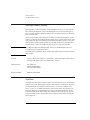
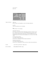
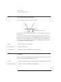
Safety Symbols.
CAUTION
Typographical Conventions.
The following conventions are used in this book:
The caution sign denotes a hazard. It calls attention
to a procedure which, if not correctly performed or
adhered to, could result in damage to or destruction
of the product. Do not proceed beyond a caution
sign until the indicated conditions are fully understood and met.
Key type for keys or text located on the keyboard or
instrument.
WARNING
The warning sign denotes a hazard. It calls attention to a procedure which, if not correctly performed or adhered to, could result in injury or loss
of life. Do not proceed beyond a warning sign until
the indicated conditions are fully understood and
met.
The instruction manual symbol. The product is marked with this warning symbol
when it is necessary for the user to refer
to the instructions in the manual.
The laser radiation symbol. This warning
symbol is marked on products which have
a laser output.
The AC symbol is used to indicate the
required nature of the line module input
power.
The ON symbols are used to mark the
positions of the instrument power line
switch.
The OFF symbols are used to mark the
positions of the instrument power line
switch.
The CE mark is a registered trademark of
the European Community.
The CSA mark is a registered trademark of
the Canadian Standards Association.
The C-Tick mark is a registered trademark
of the Australian Spectrum Management
Agency.
ISM1-A
This text denotes the instrument is an
Industrial Scientific and Medical Group 1
Class A product.
iii
Softkey type for key names that are displayed on
the instrument’s screen.
Display type for words or characters displayed on the
computer’s screen or instrument’s display.
User type for words or characters that you type or
enter.
Emphasis type for words or characters that emphasize some point or that are used as place holders for
text that you type.
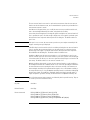
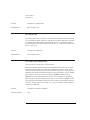
General Safety Considerations
General Safety Considerations
This product has been designed and tested in accordance with the standards listed on the Manufacturer’s Declaration of Conformity, and has been supplied in a safe condition. The documentation contains information and warnings that must be followed by the user to ensure safe
operation and to maintain the product in a safe condition.
Install the instrument according to the enclosure protection provided.
This instrument does not protect against the ingress of water.
This instrument protects against finger access to hazardous parts within the enclosure.
iv
General Safety Considerations
WARNING
If this product is not used as specified, the protection provided by the equipment could be
impaired. This product must be used in a normal condition (in which all means for protection are
intact) only.
WARNING
No operator serviceable parts inside. Refer servicing to qualified service personnel. To prevent
electrical shock do not remove covers.
WARNING
This is a Safety Class 1 Product (provided with protective earth). The mains plug shall only be
inserted in a socket outlet provided with a protective earth contact. Any interruption of the
protective conductor inside or outside of the instrument is likely to make the instrument dangerous.
Intentional interruption is prohibited.
WARNING
To prevent electrical shock, disconnect the instrument from mains before cleaning. Use a dry cloth
or one slightly dampened with water to clean the external case parts. Do not attempt to clean
internally.
CAUTION
Fiber-optic connectors are easily damaged when connected to dirty or damaged cables and
accessories. The Agilent 8614x series’s front-panel INPUT connector is no exception. When you
use improper cleaning and handling techniques, you risk expensive instrument repairs, damaged
cables, and compromised measurements. Before you connect any fiber-optic cable to the
Agilent 8614x series, refer to “Cleaning Connections for Accurate Measurements” on page 6-8.
CAUTION
This product complies with Overvoltage Category II and Pollution Degree 2.
CAUTION
Do not use too much liquid in cleaning the optical spectrum analyzer. Water can enter the frontpanel keyboard, damaging sensitive electronic components.
CAUTION
VENTILATION REQUIREMENTS: When installing the product in a cabinet, the convection into and
out of the product must not be restricted. The ambient temperature (outside the cabinet) must be
less than the maximum operating temperature of the product by 4× C for every 100 watts
dissipated in the cabinet. If the total power dissipated in the cabinet is greater than 800 watts,
then forced convection must be used.
CAUTION
Install the instrument so that the detachable power cord is readily identifiable and is easily reached
by the operator. The detachable power cord is the instrument disconnecting device. It disconnects
the mains circuit from the mains supply before other parts of the instrument. The front panel switch
v
General Safety Considerations
is only a standby switch and is not a LINE switch. Alternatively, an externally installed switch or
circuit breaker (which is readily identifiable and is easily reached by the operator) may be used as
a disconnecting device.
CAUTION
Always use the three-prong AC power cord supplied with this instrument. Failure to ensure
adequate earth grounding by not using this cord may cause instrument damage.
CAUTION
Do not connect ac power until you have verified the line voltage is correct as described in “Line
Power Requirements” on page 1-10. Damage to the equipment could result.
CAUTION
This instrument has autoranging line voltage input. Be sure the supply voltage is within the
specified range.
CAUTION
The Agilent 8614xB contain a light source classified, according to IEC 60825-1.
CAUTION
Use of controls or adjustment or performance of procedures other than those specified herein may
result in hazardous radiation exposure.
vi
Contents
1 Getting Started
Product Overview 1-2
Setting Up the Analyzer 1-8
Making a Measurement 1-12
The Menu Bar 1-15
The Softkey Panels 1-16
Laser Safety Information 1-27
Product Options and Accessories 1-28
2 Using the Instrument
Setting Up Measurements 2-2
Calibrating Wavelength Measurements 2-13
Saving, Recalling, and Managing Files 2-18
Analyzing Measurement Data 2-26
Analyzer Operating Modes 2-29
3 Function Reference
4 Remote Front Panel Operation
Remote Front Panel 4-2
5 Status Listings
Overview 5-2
Error Reporting Behavior 5-4
SCPI-Defined Errors 5-5
OSA Notices 5-16
OSA Warnings 5-17
Application-Specific Warnings 5-29
OSA Status Errors 5-35
OSA Errors 5-36
Firmware Errors 5-38
6 Maintenance
Changing the Printer Paper 6-2
Printer Head Cleaning Procedure 6-4
Cleaning Connections for Accurate Measurements 6-8
Returning the Instrument for Service 6-21
Contents-1
Contents
7 Specifications and Regulatory Information
Definition of Terms 7-3
Specifications 7-5
Regulatory Information 7-19
Declaration of Conformity 7-20
Contents-2
1
Product Overview 1-2
Setting Up the Analyzer 1-8
Making a Measurement 1-12
The Menu Bar 1-15
The Softkey Panels 1-16
Laser Safety Information 1-26
Product Options and Accessories
Getting Started
1-27
Getting Started
Product Overview
Product Overview
The 8614xB series of optical spectrum analyzers provide fast, accurate, and comprehensive measurement capabilities for spectral analysis.
• Full-featured SCPI commands for programming instruments over LAN
• Display-off feature for making faster measurements
• Remote file saving and printing for outputting measurement results
• Filter mode for accurate and flexible measurements
• Built-in applications for accelerating test times
Filter Mode
The Agilent 86146B filter mode allows single dense wavelength division multiplexing (DWDM) to
be isolated and routed to external test equipment. The filter mode capability is built-in to internal
applications to allow for fast and easy implementation of channel dropping. For Agilent 86146B
instruments, this mode also allows the ability to measure time resolve chirp (TRC).
Built-in Applications
Built-in applications allow fast, repeatable measurements for WDM systems, lasers, amplifiers,
and passive components. These applications can be added through a firmware upgrade.
WDM Application
This application allows you to measure DWDM sub-system components, (such as transmission
sub-systems, optical add/drop multiplexers, and multiplexers/de-multiplexers) for parameters
such as optical signal-to-noise ratio (OSNR), channel wavelength, channel power, and span tilt.
Passive Component Test Application
This application simplifies the testing of passive components, such as filters, couplers, and isolators by defining a test plan that measures parameters such as insertion and return loss, bandwidth, and filter shape.
Source Test Application
This application offers automated optical source and laser characterization.
1-2
Getting Started
Product Overview
Amplifier Test Application
This application simplifies the process of characterizing gain and noise figure of optical amplifiers
such as EDFA’s, SOA’s and Raman amplifiers.
1-3
Getting Started
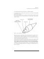
Product Overview
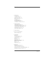
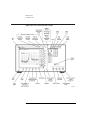
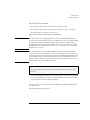
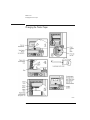
Agilent 8614xB Front and Rear Panels
1-4
Getting Started
Product Overview
1-5
Getting Started
Product Overview
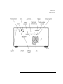
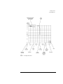
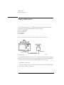
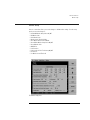
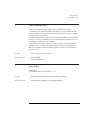
Optical Spectrum Analyzer Display
Figure 1-1. Optical Spectrum Analyzer Display
1-6
Getting Started
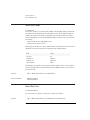
Product Overview
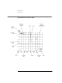
Figure 1-2. Display Annotations
1-7
Getting Started
Setting Up the Analyzer
Setting Up the Analyzer
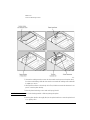
Step 1. Receive and Inspect the Shipment
1-8
Getting Started
Setting Up the Analyzer
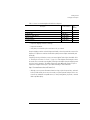
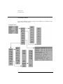
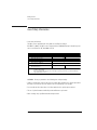
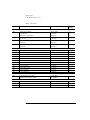
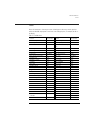
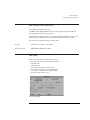
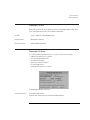
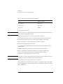
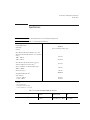
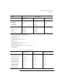
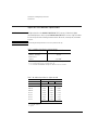
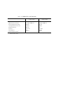
Table 1-1. Items in a Standard Agilent 8614xB Series Shipment
Description
BNC Cable (24 inches)
GPIB Cable
FC/PC Dust Cap
English User’s Guide Manual
Application Guide
Programming Guide
Product Number
8120-1839
8120-3444
1401-0291
86140-90U03
86140-90071
86140-90069
Item
Quantity
1
1
2
1
1
1
• Inspect the shipping container for damage.
• Inspect the instrument.
• Verify that you received the options and accessories you ordered.
Keep the shipping container and cushioning material until you have inspected the contents of the
shipment for completeness and have checked the optical spectrum analyzer mechanically and
electrically.
If anything is missing or defective, contact your nearest Agilent Technologies Sales Office. Refer
to “Returning the Instrument for Service” on page 6-21. If the shipment was damaged, contact
the carrier, then contact the nearest Agilent Technologies Sales Office. Keep the shipping materials for the carrier’s inspection. The Agilent Technologies Sales Office will arrange for repair or
replacement at Agilent Technologies’ option without waiting for claim settlement.
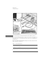
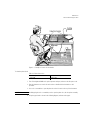
Step 2. Connect Accessories and Power Cord
• Although you can operate all instrument functions using only the front-panel keys, and trackball on portable models, these accessories make your optical spectrum analyzer easier to use.
Connect any standard PC-compatible mouse (or other pointing device), keyboard, or external
VGA-compatible display.
1-9
Getting Started
Setting Up the Analyzer
CAUTION
Do not stack other objects on the keyboard; this will cause self-test failures on power-on.
r You can connect a PCL-language printer (for example, an HP1 LaserJet) to the instrument’s rear
panel Parallel connector. Use a parallel Centronics printer cable, such as an HP C2950A (2 m) or
HP C2951A (3 m).
r The line cord provided is matched by Agilent Technologies to the country of origin on the order.
Refer to “Accessories” on page 1-28.
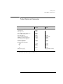
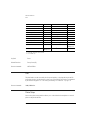
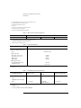
Table 1-2. Line Power Requirements
Voltage
100/ 115/ 230/ 240 V ~
Frequency
50 / 60 Hz
1. HP and Hewlett-Packard are U.S. registered trademarks of Hewlett-Packard Company.
1-10
Getting Started
Setting Up the Analyzer
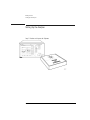
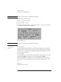
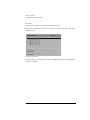
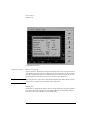
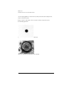
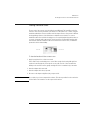
Step 3. Apply Power to Instrument
• Press the power switch at the lower left-hand corner of the front panel.
• After a short initialization period, the display will look similar to the picture on this page.
• Allow the instrument to warm up for at least 1 hour.
Step 4. Clean Connectors and Prepare for Measurements
CAUTION
Fiber-optic connectors are easily damaged when connected to dirty or damaged cables and
accessories. The front-panel INPUT connector of the Agilent 8614x series is no exception. When
you use improper cleaning and handling techniques, you risk expensive instrument repairs,
damaged cables, and compromised measurements. Before you connect any fiber-optic cable to
the Agilent 8614x series optical spectrum analyzer, refer to “Cleaning Connections for Accurate
Measurements” on page 6-8.
CAUTION
A front-panel connector saver is provided with Agilent 8614x series instruments. Attach the
connector saver to the front-panel INPUT connector of the instrument. You can now make your
connections to the connector saver instead of the instrument. This will help prevent damage to the
front-panel INPUT connector of the instrument. Damage to the front-panel INPUT connector is
expensive in terms of both repair costs and down-time. Use the front-panel connector saver to
prevent damage to the front-panel INPUT connector.
Note
All product specifications apply to measurements made without using the front-panel connector saver.
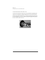
• After the instrument has warmed up for at least 1 hour, perform an auto align by pressing the
front panel Auto Align button. This will ensure optimal amplitude accuracy, and can correct for
any mis-alignment caused by the instrument shipment.
To learn more about this or any Agilent Technologies Optical Test and Measurement Products,
visit our web site at
http://www.agilent.com/comms/optical
1-11
Getting Started
Making a Measurement
Making a Measurement
This procedure will introduce you to the Agilent 8614x series optical spectrum analyzer front
panel controls. By following this procedure you will do the following:
•
•
•
•
Perform an auto alignment
Perform a peak search
Use a delta marker
Print the display
Refer to “The Menu Bar” on page 1-15 and “The Softkey Panels” on page 1-16.
Instrument setup
A source signal must be present at the input of the optical spectrum analyzer. In this procedure a
Fabry-Perot laser is used as the source. You can use another source or the optional 1310/1550
nm eeled. If another source is being used, the display will differ from those shown.
To set the OSA to a known state
• Press the front-panel Preset key to set the instrument to a known state. For a complete description of preset conditions, see page 3-59.
1-12
Getting Started
Making a Measurement
To perform an Auto Align
For maximum amplitude accuracy, perform an automatic alignment whenever the optical spectrum analyzer has been moved, subjected to large temperature changes, or following warm-up.
See “Auto Align” on page 3-9 for more information.
1 Connect a fiber from the source to the input connector of the optical spectrum analyzer. Be sure
to follow the good connector practices described in “Cleaning Connections for Accurate
Measurements” on page 6-8.
2 Enable the source. Press Markers > Peak Search to find the peak signal power.
3 Press the front-panel Auto Align key to optimize the detection of the incoming signal. This takes a
few moments to complete.
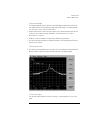
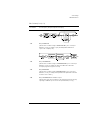
To perform a peak search
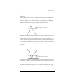
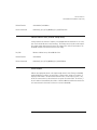
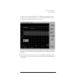
4 Press the front-panel Auto Meas key to locate and zoom-in on the signal. Please wait until the Auto
Measure routine is complete. A marker is placed on the peak of the displayed signal.
Trace with normal marker.
To zoom in on the signal
Press the Span softkey and then use the knob, step keys, or numeric keypad to zoom in on the
signal.
1-13
Getting Started
Making a Measurement
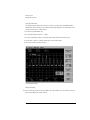
Using the delta marker
The optical spectrum analyzer has four types of markers; normal markers, bandwidth markers,
delta markers and noise markers. The marker currently being displayed is a normal marker. In the
next step we will use it as a delta marker.
5 Press the front-panel Markers key.
6 Press the More Marker Functions.... softkey.
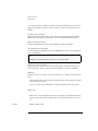
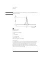
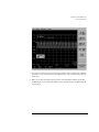
7 Press the Delta Marker softkey to activate the delta marker and the active function area.
8 Use the knob, step keys or numeric entry pad to move the delta marker.
9 The reference marker remains stationary.
Trace with delta marker.
Printing the display
10 Press the Print key to print a copy of the display. The output will be sent to the internal or external
printer, depending on the printer selected.
1-14
Getting Started
The Menu Bar
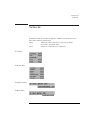
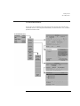
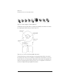
The Menu Bar
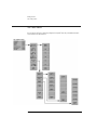
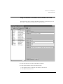
The Menu bar includes the File, Measure, Application, and Options drop-down menus. Each
menu selection includes a descriptive label.
(Action)
Indicates the selection will perform an action such as making a
measurement or printing the display.
(Panel)
Indicates the selection will open a softkey panel.
The File Menu
The Measure Menu
The Applications Menu
The Options Menu
1-15
Getting Started
The Softkey Panels
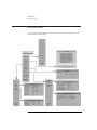
The Softkey Panels
You can access the softkey panels using either the front-panel keys or the menu bar. This section
includes brief descriptions of the following menus. See Chapter 3, “Function Reference” for additional information on each of the OSA functions.
The Amplitude Menus 1-17
The Applications Menus 1-17
The Bandwidth/Sweep Menus 1-19
The Markers Menus 1-20
The Save/Recall Menus 1-21
The Systems Menus 1-22
The Traces Menus 1-24
The Wavelength Menus 1-25
1-16
Getting Started
The Softkey Panels
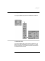
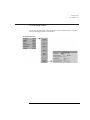
The Amplitude Menus
You can access the Amplitude softkeys using the front-panel Amplitude key or the Measure
menu Amplitude selection on the menu bar.
The Applications Menus
You can access the Applications (Appl’s) softkeys by using the front-panel Appl’s key or the
Applications menu Launch an Installed Application section on the menu bar. For a complete
description of the applications, refer to the Agilent 8614xB Series Measurement Applications
User’s Guide that came with your instrument.
1-17
Getting Started
The Softkey Panels
1-18
Getting Started
The Softkey Panels
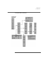
The Bandwidth/Sweep Menus
You can access the Bandwidth/Sweep softkeys by using the front-panel Bandwidth/Sweep key
or the Measure menu Bandwidth/Sweep selection on the menu bar.
1-19
Getting Started
The Softkey Panels
The Markers Menus
You can access the Markers softkeys by using the front-panel Markers key or the Measure menu
Markers selection on the menu bar.
1-20
Getting Started
The Softkey Panels
The Save/Recall Menus
You can access the Save/Recall softkeys and setup panels by using the drop-down File menu
Save/Recall selection or the front-panel Save/Recall key. Use these functions to save, recall and
print the measurement results.
1-21
Getting Started
The Softkey Panels
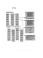
The Systems Menus
You can access the System softkeys by using the front-panel System key or the Options menu
System selection on the menu bar.
1-22
Getting Started
The Softkey Panels
The Systems Menus, continued....
1-23
Getting Started
The Softkey Panels
The Traces Menus
You can access the Traces softkeys by using the front-panel Traces key or the Measure menu
Traces selection on the menu bar.
1-24
Getting Started
The Softkey Panels
The Wavelength Menus
You can access the Wavelength softkeys by using the front-panel Wavelength key or the Measure menu Wavelength selection on the menu bar.
1-25
Getting Started
Laser Safety Information
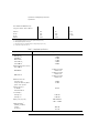
Laser Safety Information
• Laser Safety Information
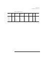
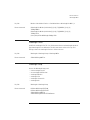
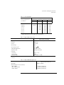
The light sources specified by this user guide are classified according to
IEC 60825-1 (2001). The light sources comply with 21 CFR 1040.10 except for deviations pursuant to Laser Notice No. 50, dated 2001-July-26
Laser type
W avelength
M ax. CW output pow er *
Beam w aist diam eter
Num erical aperture
Laser class according to
IEC 60825-1 (2001)
M ax. perm issible
CW output pow er **
*
**
Edge em itting LED (EELED)
1310nm
1550 nm
50 µW
9 µm
0.1
1
15,6m W
10m W
M ax. CW output power means the highest possible optical CW pow er that the laser source can
produce at its output.
M ax. perm issible CW output power is the highest optical power that is perm itted within the
appropriate IEC laser class.
WARNING - Please pay attention to the following laser safety warnings:
• Under no circumstances look into the end of an optical cable attached to the optical output when
the device is operational. The laser radiation can seriously damage your eyesight.
• Do not enable the laser when there is no fiber attached to the optical output connector.
• The use of optical instruments with this product will increase eye hazard.
• Refer servicing only to qualified and authorized personnel.
1-26
Getting Started
Product Options and Accessories
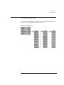
Product Options and Accessories
Options
Agilent 86142B, 86146B
Benchtop
Agilent 86143B, 86145B
Portable
Opt. 001
Opt. 002
Opt. 004
Opt. 005
Opt. 006
Opt. DPCa
Included
Included
Included
Included
------------Opt. 006
Not Applicable
Included
Included
Included
Included
Standard
Opt. 013
Opt. 014
Opt. 017
Standard
Opt. 013
Opt. 014
Opt. 017
Instrument System Options
Current Source
White Light Source
Built-in 1310 & 1550 nm EELED Source
Built-in 1550 nm EELED Source
Wavelength Calibrator
Time Resolved Chirp Application
DWDM Spectral Analysis Application
Passive Component Test Application
Amplifier Test Application
Source Test Application
Alternative Connector Interface
FC/PC
DIN
ST
SC
Opt. 025 (Agilent 86143B)
Multimode Fiber Inputb
Certificate of Calibration
Included
Included
a. Option available for 86146B only.
b. 50µm multimode input available on Agilent 86143B OSA’s only.
1-27
Getting Started
Product Options and Accessories
Table 1-3. Accessories
Option
Description
Product Number
Item
Quantity
08154-61702
1401-0291
1250-3175
08154-61703
1401-0291
08154-61704
1401-0291
08154-61708
1401-0291
3
3
1
3
3
3
3
3
3
8120-1351
8120-1369
8120-1689
8120-1378
8120-2104
8120-3997
8120-4211
8120-4753
8120-5182
8120-6868
8120-6979
8120-8376
1
1
1
1
1
1
1
1
1
1
1
1
86140-90067
86140-90066
1
N/A
N/A
N/A
1
1
1
Connector Accessories
012
013
014
017
FC/PC Connector Adapter
FC/PC Dust Cap
Angled to Flat, FC/PC Adapter
DIN Optical Connector Adapter
DIN Dust Cap
ST Optical Connector Adapter
ST Dust Cap
SC Optical Connector Adapter
SC Dust Cap
Power Selection
900
901
902
903
906
912
917
918
919
920
921
922
Power Cord (United Kingdom)
Power Cord (Australia, New Zealand, China)
Power Cord (Europe)
Power Cord (United States)
Power Cord (Switzerland)
Power Cord (Denmark)
Power Cord (South Africa, India)
Power Cord (Japan)
Power Cord (Israel)
Power Cord (Argentina)
Power Cord Chilean)(
Power Cord (China)
Documentation and Manuals
ABC
Traditional Chinese User’s Guide
Traditional Chinese Application Guide
Certification of Calibration and Service
1BM
UK6
W30
Standard Commercial Calibration Certificate
Commercial Calibration Certificate with Test Data
Extended Warranty to 3 Years Return for Service
1-28
Getting Started
Product Options and Accessories
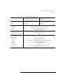
Table 1-4. Available Fiber Sizes
Model
Number
Optical
Input
Option 002a
(White Light
Source)
Option 004a
(1310/1550
EELED)
Option 005a
(1550 EELED)
Option 006
(Calibrator)
Photodiode
Input
Mono Output
1
86143B
9 µm
N/A
N/A
N/A
9 µm
N/A
N/A
Opt 025
50 µm
86145B
9 µm
N/A
N/A
N/A
9 µm
N/A
N/A
86142B
9 µm
62,5 µm
9 µm
9 µm
9 µm
N/A
N/A
86146B
9 µm
62,5 µm
9 µm
9 µm
9 µm
50 µm
9 µm
9 µm
a. Options 002, 004, and 005 are exclusive
1-29
Getting Started
Product Options and Accessories
Table 1-5. Additional Parts and Accessories
Printer Paper (5 rolls/box)
Additional Connector Interfaces
External 10 dB Attenuator (FC/PC)
Rack-Mount Flange Kit
Transit Case
Soft Carrying Case
BenchLink Lightwave Softwarea
Agilent Benchtop OSA
86142B, 86146B
9270-1370
See Agilent 81000 series
Opt. 030
Opt. AX4
9211-2657
N/A
Standard
Agilent Portable OSA
86143B, 86145B
9270-1370
See Agilent 81000 series
Opt. 030
N/A
9211-5604
Opt. 042
Standard
a. Agilent N1031A BenchLink Lightwave allows transfer of measurement results over a GPIB Interface to a PC for the purposes of archiving,
printing, and further analysis.
1-30
Getting Started
Product Options and Accessories
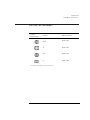
Front Panel Fiber-Optic Adapters
Front Panel
Fiber-Optic Adapter
Description
Agilent Part Number
FC/PCa
08154-61702
SC
08154-61708
DIN
08154-61703
ST
08154-61704
a. The FC/PC is the default front-panel optical connector.
1-31
Getting Started
Product Options and Accessories
1-32
2
Setting Up Measurements 2-2
Calibrating Wavelength Measurements 2-13
Saving, Recalling, and Managing Files 2-18
Analyzing Measurement Data 2-26
Analyzer Operating Modes 2-29
Using the Instrument
Using the Instrument
Setting Up Measurements
Setting Up Measurements
This section contains the following information that will help you set up a wavelength measurement:
• Adjusting Setup Conditions
• Operating the Internal White Light Source
• Averaging Traces
• Setting Video Bandwidth
• Using Span to Zoom In
• Setting the Sensitivity
• Triggering a Measurement
• Moving the Active Function Area
• Indicating an Update is Needed
2-2
Using the Instrument
Setting Up Measurements
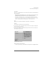
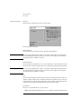
Adjusting Setup Conditions
Setup panels allow you to adjust setup conditions which are not frequently changed. Refer to
“Preset” on page 3-59.
Using the softkeys
Arrows allow you to navigate from field to field in the dialog box. The highlighted parameter can
be changed. The front-panel number keys, step keys, and knob allows the user to enter a
numeric value in the highlighted field.
Select selects the highlighted parameter. You can enter values for a selected parameter using the
front panel knob or numeric entry pad.
Defaults resets the parameters to their default condition.
Close Panel saves the current setup and returns you to the previous menu.
2-3
Using the Instrument
Setting Up Measurements
Operating the Internal White Light Source
For Option 002 only
Option 002 provides a built-in white light source which is a stable, broadband light source for
swept-wavelength stimulus response testing from 900 nm to 1700 nm. The light source is ideal
to perform stimulus-response measurements, and measure photodetector responsivity. Refer to
“Light Source” on page 3-29.
Note
Although the light source’s lamp lasts an exceptionally long time, turn off the light when not in use
to extend the lamp’s lifetime. On the front panel, press System, Optimum, Light Source, Select off.
1 From the front panel, press System > Options > Light Source > Select Off.
Performing Stimulus-Response Measurements
Stimulus-response measurements characterize optical components for loss (or gain) versus
wavelength. You can characterize devices such as couplers, switches, filters, fibers, and amplifiers.
To perform stimulus-response measurements, you must have an amplitude-stable broadband
light source. Although a white-light source provides the widest wavelength input for stimulusresponse measurements, you can also use an LED or the spontaneous emission from an optical
amplifier.
The displayed response is a convolution of the analyzer’s resolution bandwidth and the amplitude
response of the device under test. Because of this convolution, the analyzer’s resolution bandwidth affects both dynamic range and the ability to resolve large amplitude changes versus
wavelength. Wide resolution bandwidths increase the ability to resolve large amplitude changes.
You can display two responses at the same time. The output response versus wavelength is displayed. The displayed trace shows the ratio of the output power to the input power expressed as
a logarithm (dB).
response (dB) = 10 log(output power/input power)
Making ratioed measurements is sometimes referred to as normalization. Normalized measurements are used to negate wavelength dependencies in the source. The ratio is achieved through
simple trace subtraction using logarithmic amplitude scales. This is possible because of the following logarithmic equality:
log(A/B) = (logA - logB)
1 Connect the Light Source Output to the Monochromator Input using the short 62.5/125 µm fiber.
The standard connector interface is FC/PC.
2-4
Using the Instrument
Setting Up Measurements
Averaging Traces
Trace averaging improves your measurement repeatability by smoothing out noise. For measurements involving slow polarization scrambling, using video filtering to improve repeatability will
require a very narrow video bandwidth (less than 10 Hz). This would result in a long measurement time, where trace averaging would be faster. Refer to “Averaging” on page 3-13.
1 From the front panel, press Traces > Averaging.
2 Toggle to select the Averaging on or off.
3 Select from the 10, 20, 50 or 100 softkeys or use the knob, step keys, or numeric entry pad to
enter the desired average count.
Note
For measurements with fast polarization scrambling, video filtering (adjusting video bandwidth) is
generally faster than trace averaging for similar repeatability requirement.
2-5
Using the Instrument
Setting Up Measurements
Setting Video Bandwidth
Video bandwidth filtering occurs after the detection of the light. In the auto coupled mode, the
video bandwidth has an extremely wide range. This allows the instrument to avoid unnecessary
filtering that would reduce the sweep speed more than required. Refer to “Video BW” on
page 3-91.
The instrument has two detection techniques: peak (auto mode) and sample (manual mode).
Peak detection is beneficial for maintaining the fastest sweep times and displaying narrow aspect
ratio signals. Sample detection is beneficial for obtaining best measurement accuracy and measuring low level signals.
Peak detection finds and displays the maximum signal level present during each trace point interval. Peak detection is used if video filtering is not required to achieve the desired level of sensitivity. However, there is one exception: if an auto-coupled sweep time is limited by either maximum
motor speed or a 50 ms auto-coupling limit, then sample detection is used with as narrow a digital video bandwidth as possible in order to achieve maximum sensitivity for the chosen sweep
time. This exception only applies when both sweep time and video bandwidth are auto-coupled.
Sample detection displays a filtered version of the sampled data at the end of each trace point
interval. The filter function is varied with the video bandwidth function from 100 mHz to 3.0 kHz,
or the bandwidth of the currently selected transimpedance amplifier, whichever is less. Increased
filtering provides greater sensitivity.
The detection mode is automatically determined by the instrument. You can adjust the settings of
video bandwidth, sensitivity, or sweep time to obtain the desired detection mode. Sample detection can be forced at any time by putting video bandwidth in manual. Peak detection can usually
be obtained by placing sensitivity and video bandwidth in auto.
The following functions affect video bandwidth:
• changing the sensitivity value
• changing the reference level
• turning auto ranging on or off
The range of video bandwidths available in auto mode is much greater than can be set manually
from the front panel. A lower video bandwidth value requires a longer sweep time. Because of
the interdependence between the video bandwidth and sensitivity, it is recommended that either
the sensitivity or the video bandwidth be changed, whichever is the most important to the measurement task being performed.
To reduce noise, you can select a narrower video bandwidth to improve repeatability and sensitivity or select a wider video bandwidth to shorten overall measurement time. This selection
allows the choice between repeatability and measurement time based on your measurement
requirements. The narrower the video bandwidth, the longer the sweep time.
2-6
Using the Instrument
Setting Up Measurements
1 From the front panel, press Bandwidth/Sweep > Video BW.
2 Toggle to select the video bandwidth automatically or manually.
3 Use the knob, step keys, or numeric entry pad to enter the desired value.
Note
For measurements with slow polarization scrambling, use trace averaging to improve
measurement repeatability. Trace averaging is faster than video filtering for the slow polarization
scrambling application.
Using Span to Zoom In
To see a more detailed view of the device’s response, decrease the wavelength span to expand
the trace. This will enable you to precisely focus in on the desired measurement area. Refer to
“Span” on page 3-79.
Press Wavelength > Span and reduce the span by entering the value of 2 nm.
2-7
Using the Instrument
Setting Up Measurements
Setting the Sensitivity
Setting sensitivity requests the lowest amplitude signal that can be measured relative to the highest amplitude signal displayed. It is defined as the signal that is six times the RMS noise. The minimum setting is –100 dB. An error will be reported for values outside of this range and the
sensitivity will round to the nearest valid sensitivity. Refer to “Sensitivity” on page 3-74.
Manual allows manual input of sensitivities and enables auto gain ranging. The “top of screen”
and the sensitivity setting determines the requested dynamic range. The system will sweep once
per gain stage and may require up to three sweeps to achieve the requested dynamic range.
Auto automatically chooses a sensitivity and a single gain range based on “top of screen”. This
will result in approximately 40 dB of dynamic range.
The sweep time that is displayed in the lower portion of the display is the time for the OSA to
sweep over one gain stage. The OSA may take up to three sweeps in three different gain stages
to make the measurement. This depends on the settings for sensitivity, reference level, auto
range and also the particular device being measured. The final data trace is a blended composite
of each trace taken in the different gain stages.
An increase in sensitivity may also require a narrower video bandwidth, which will slow the
sweep speed. Normally, the optical spectrum analyzer selects the greatest sensitivity possible
that does not require amplification changes during the sweep. If you manually increase the sensitivity level, the sweep pauses to allow this change in gain.
The settings for sensitivity, video bandwidth and sweep time interact. If the sensitivity is set to
manual, the video bandwidth and sweep time may be forced to Auto mode. If the video bandwidth is set to manual, the sensitivity and sweep time may be forced to Auto. If the sweep speed
is set to manual and is set too fast, the over sweep indicator will come on in the display area.
Since these settings interact, it is recommended that only one of the settings be changed, whichever setting is most important to the measurement task being performed.
Press Amplitude, Sensitivity, toggle to manual, and enter a value.
2-8
Using the Instrument
Setting Up Measurements
Triggering a Measurement
Triggering a measurement synchronizes the start of the sweep to an internally generated trigger
signal. Internal triggering ensures continuously triggered sweeps with the shortest delay between
sweeps. Refer to “Trigger Mode, Internal” on page 3-88.
In some measurements, the spectrum at a particular time within the modulation period is more
important than the average spectrum. Gated triggering can be used to synchronize the data
acquisition portion of the OSA to a gating trigger connected to the rear-panel EXT TRIG IN connector. Gated triggering requires a TTL-compatible signal with a minimum of 0 Vdc and a maximum of +5 V.
Gated triggering ignores the spectrum when the trigger input is low. It usually is used in conjunction with the Max Hold function during several sweeps.
Gated triggering is used to select data samples containing valid information. When the gating
signal is high, the data sample is accepted. When the gating signal is low, the data sample is
replaced by a data point with a value of –200 dBm. Processing continues according to the functions selected, such as, video bandwidth, max hold, and so forth.
If the low level exists for longer that the time needed for the grating to move from one trace point
to the next, then the trace will have “gaps”. There are two ways to eliminate the gaps. You can
increase the sweep time to at least:
(1.2–2 times the product trace length) ¥ (the longest “low level” period)
2-9
Using the Instrument
Setting Up Measurements
The display will have at least one data sample marked as valid (high level) per trace point. Or else
you can use the Max Hold function to complete a trace over several sweeps. Multiple sweeps fill
the gaps because the high and low levels of the gating signal occur independent of the grating
position.
Gated triggering has no time limit for the high or low level. It can be used to characterize pulses
as narrow as a few microseconds, or to obtain a spectrum whose timing exceeds the maximum
6.5 ms delay of the ADC trigger mode.
1 On the front panel press Bandwidth > Sweep > More BW Sweep > Functions > Trigger Mode.
2 Select from int, gated, and ext.
2-10
Using the Instrument
Setting Up Measurements
Moving the Active Function Area
The active function area on the display can be moved to eight different locations. This allows you
to place the active area in a location that will not interfere with the trace information. Refer to
“Active Function Area Assist” on page 3-2.
1 Press the front-panel System key.
2 Press the Move Active Area softkey. Each press of the softkey moves the active function area to
one of eight onscreen locations.
2-11
Using the Instrument
Setting Up Measurements
Indicating an Update is Needed
This feature alerts you to take a sweep after changing any sweep related parameters when the
analyzer is not in sweep mode. For example, if you change the resolution bandwidth, the new
resolution bandwidth is displayed on the bottom of the screen, but the trace data displayed on
the screen used the previous resolution bandwidth value.
Changing the following sweep parameters will set the Update Needed Indicator to on:
•
•
•
•
•
•
•
•
•
•
•
•
•
•
•
•
•
•
•
•
•
•
•
start wavelength
stop wavelength
sensitivity auto/manual
auto range enable/disable
sensitivity
video bandwidth auto/manual
resolution bandwidth
video bandwidth
gated sweep enable/disable
sweep continuous/single
sweep time auto/manual
sweep time
sweep trace length
reference level
dB per division
reference level position
Y scale linear/log mode
amplitude correction enable/disable
current active ampcorr correction set
ampcor interpolation method
vacuum or air
wavelength offset
number of averages for trace averaging
The Update Needed Indicator, “*’”, is displayed in the upper right hand corner of the graticule.
After a sweep is taken, the Update Needed Indicator will be set to off.
2-12
Using the Instrument
Calibrating Wavelength Measurements
Calibrating Wavelength Measurements
Environmental variations such as air pressure, temperature, and humidity can affect the index of
refraction of air in the monochromator of the optical spectrum analyzer (OSA). This section discusses calibration methods that you can use to improve the wavelength accuracy in the Agilent
8614xB OSA’s. Refer to “Calibration” on page 3-16 and to “Calibrator Multi-Pt Align” on
page 3-16.
Note
Many aspects of remotely programming the optical spectrum analyzers are discussed in Product
Note 86140-2R, Wavelength Calibration for the 86140X Series Optical Spectrum Analyzers
(Literature part number 5980-0043E).
Overview
Wavelength calibration routines improve wavelength accuracy by determining errors and correcting them with offsets, using linear interpolation when necessary. For maximum wavelength
accuracy, calibration points spaced a maximum of 10 nm apart are recommended.
You can perform a wavelength calibration by using one of the following methods:
•
•
•
•
•
Manual Method using Internal Calibrator
Remote Method using Internal Calibrator
Manual Method using an External Single Wavelength Source
Remote Method using an External Single Wavelength Source
External Multipoint Wavelength Calibration
These calibration routines should only be performed after the instrument’s temperature has been
stabilized by a minimum of 1 hour of continuous operation.
2-13
Using the Instrument
Calibrating Wavelength Measurements
Internal Wavelength Calibration
The optional internal calibrator (1513 to 1540 nm) provides a convenient method for increasing
wavelength accuracy when used with an internal Enhanced Wavelength Calibration (EWC) process. The wavelength accuracy of the OSA will be ±0.2 nm over the full wavelength range of the
instrument, with ±10 pm over 1480 to 1570 nm and ±25 pm accuracy over 1570 to 1620 nm.
The EWC range can be selected for either the “full” OSA range of 605 nm to 1670 nm, or the
“telecom” range of 1270 to 1670 nm, a smaller span more relevant to telecommunications. EWC
must be enabled for the wavelength accuracy specifications to apply in the range selected. Setting the range to FULL will require a longer calibration time for an internal calibration, but will
provide enhanced wavelength accuracy over the full range.
Manual method using the internal calibrator
1 Access the EWC setup panel:
System > More System Functions > Service Menu > Adv Service Functions > More Adv
Service Menu > Enhanced Wvl Cal Setup
2 Enable the function, if necessary, and select the desired calibration range.
3 Clean all connectors and connect the internal calibrator to the OSA input.
4 Access the Wavelength Calibration setup panel:
System >Calibration > Wavelength Cal Setup
5 Set the signal source to Calibrator.
6 Press Perform Calibration.
Remote method using the internal calibrator
CALibration:WAVelength:EWC:FUNCtion ON
CALibration:WAVelength:EWC:RANGe TELE
CALibration:WAVelength:INTernal:NORMal
2-14
!Enable enhanced wavelength calibration.
!Select telecom (1270-1670) nm range for
enhanced wavelength calibration.
!Perform internal wavelength calibration.
!The internal calibrator must be connected
before sending this command.
Using the Instrument
Calibrating Wavelength Measurements
External Single Wavelength Calibration
Using an external single-point calibration source allows the calibration to be done at a specific
wavelength. This single wavelength user calibration can be repeated as often as necessary to
correct for environmental variations and existing multipoint wavelength offsets will be adjusted
accordingly. After a single wavelength calibration, wavelength accuracy will be ±10 pm within
10 nm of the reference signal.
The Enhanced Wavelength Calibration (EWC) process can also be used to increase the accuracy
of the single-point calibration.
Manual method using an external source
1 Connect the external source to the OSA input.
2 Auto align the OSA to the input signal.
3 Access the Wavelength Calibration setup panel:
System > Calibration > Wavelength Cal Setup
4 Select Air or Vacuum reference for the signal source.
5 Set the signal source to External.
6 Select the desired Calibration Wavelength. This wavelength must be within
±2.5 nm of the source wavelength.
7 Select Perform Calibration.
Remote method using an external source
• For a source with a single peak:
CALibration:WAVelength:VALue <param>
CALibration:WAVelength
!Set calibration wavelength
!Calibrate signal at wavelength
• For a source with multiple peaks:
CALibration:WAVelength:VALue <param>
CALCulate:MARKer[1|2|3|4]:X:WAVelength
<param>
CALibration:WAVelength:MARKer
!Set calibration wavelength
!Set marker wavelength
!Calibrate signal at marker
2-15
Using the Instrument
Calibrating Wavelength Measurements
External Multipoint Wavelength Calibration
An external multipoint wavelength calibration can be performed over any specified wavelength
range, up to and including the full wavelength range of the OSA (600 nm to 1700 nm). Narrow
measurement spans can be chosen to provide greater accuracy over a selected range. Calibrating the wavelength every 10 nm within the desired wavelength range is usually sufficient to
improve wavelength accuracy. After a multipoint wavelength calibration, wavelength accuracy
will be ±10 pm within 10 nm of each calibration wavelength. Refer to “Calibrator Multi-Pt Align”
on page 3-16.
Note
For a full explanation of external multipoint wavelength calibration, along with a sample program
to perform the calibration, refer to Product Note 86140-2, Wavelength Calibration for the 86140X
Series Optical Spectrum Analyzers (Literature part number 5980-0043E).
The following steps outline one method for an external multipoint wavelength calibration routine.
This assumes a program executed on a external PC controller. The steps outlined are those written in the program.
1 A signal is sent from a tunable laser source into a multi-wavelength meter and the OSA
simultaneously.
2 The wavelength of the input signal is measured on both instruments.
3 The two measured values are compared.
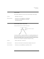
4 Taking the multi-wavelength meter readings as actual, the software calculates the error offsets at
each wavelength using the equation:
WL Error = (OSA indicated WL) – (multi-wavelength meter actual WL)
5 The previous steps are repeated over the entire wavelength range.
6 The data is averaged over narrow wavelength spans to provide a suitable correction for each
span. The example below demonstrates this technique.
Once the instrument is calibrated, the new wavelength accuracy can be maintained for many
hours without recalibration, assuming a stable temperature environment.
Tip
If the OSA is turned off, the multipoint data will be retained at the next power-on, but the internal
thermal shift can introduce inaccuracies to the calibration data. To help compensate for this, a
single point calibration using the Offset feature in the Wavelength Calibration Setup panel can be
used to adjust the multipoint data. Access this feature by selecting System > Calibration >
Wavelength Cal Setup and choosing the Offset option before running the single point calibration.
2-16
Using the Instrument
Calibrating Wavelength Measurements
To insure this offset process has provided sufficient accuracy, the wavelength readings of the
multi-wavelength meter and the OSA should be compared to verify the wavelength accuracy and
determine if a full multipoint wavelength recalibration is necessary.
2-17
Using the Instrument
Saving, Recalling, and Managing Files
Saving, Recalling, and Managing Files
The functions and methods available for saving, recalling, and managing files that contain measurement setups and results are as follows:
• Adding a Title to the Display
• Backing Up or Restoring the Internal Memory
• Saving Measurement Trace Data
• Recalling Measurement Trace Data
• File Sharing and Printing over a Network
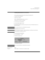
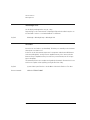
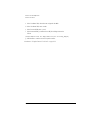
Adding a Title to the Display
Refer to “Title (Display Setup Panel)” on page 3-85 and to “Date/Time (Display Setup Panel)” on
page 3-19.
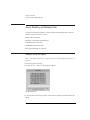
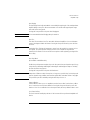
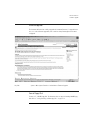
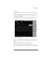
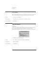
1 Press the front-panel System key.
2 Press the Set Title.... softkey. The Title Setup panel appears.
The Title Setup panel
3 To view the title on the display, press More System Functions >Display Setup and check the Title
On box.
2-18
Using the Instrument
Saving, Recalling, and Managing Files
Backing Up or Restoring the Internal Memory
1 Press the front-panel Save/Recall key.
2 Press the Backup/Restore Menu.... softkey.
Note
The auto span value will not be saved with the measurement. Refer to “Backup Internal Memory”
on page 3-13.
Softkey Panel Selections
Backup Internal Memory
a The analyzer Backup Utility screen appears asking you to insert a formatted floppy disk in the
external drive. The disk will not be viewable on a PC and no trace or measurement files can be
saved onto the disk until it is reformatted.
b The Backup Internal Memory function overwrites the floppy disk with a new image. Any existing files or catalogs on the floppy disk will be destroyed. Any successive backup operations will
overwrite the previous backup information, so only the latest backup information can be recovered through the Restore Internal Memory operation.
Restore Internal Memory
The analyzer Restore Utility screen appears. This operation will remove all files from internal
memory and replace them with files from backup floppy disks.
Saving Measurement and Trace Data
You can save measurement and trace data using the following methods:
• Fast Measurement Save Mode
• Save Setup Panel Mode
Saving Data in Fast Meas Save Mode
1 Press the front-panel Save/Recall key.
2 Press the Fast Meas SAVE softkey.
3 The instrument saves the current measurement state to internal memory as FASTSAVE.dat. Only
one FASTSAVE.dat file exists, so performing a Fast Meas Save will overwrite any currently existing
Fast Save file.
2-19
Using the Instrument
Saving, Recalling, and Managing Files
Note
The auto span value will not be saved with the measurement.
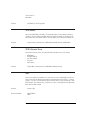
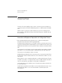
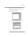
Saving Measurement and Trace Data
1 Press the front-panel Save/Recall key.
2 Press the Save Menu.... softkey.
3 The Save Setup panel opens. Refer to “Adjusting Setup Conditions” on page 2-3 for information
on changing and selecting items in the setup panel.
The Save Setup panel
Note
The auto span value will not be saved with the measurement.
Save Setup Panel
Selections
Save: Measurement
Saves the measurement data in a binary format (.dat file). This includes the traces and all measurement conditions. The dat file format can only be read by the analyzer. You will not be able to
view this file on your PC. When the file is recalled, the instrument state will be set to the same
state as when the file was saved.
Save: Trace(s) Only
The Trace(s) Only files are saved in comma separated variable (.csv) format and are auto named
starting with TR_00000.csv. State files are auto named starting with ST_00000.csv.
When the Trace(s) Only file is recalled, the trace data will be displayed under the current instrument settings.To view the instrument settings, press System > More System Functions > State
Info.
Save Traces
Selects the traces to be saved.
2-20
Using the Instrument
Saving, Recalling, and Managing Files
Save Graphics
Allows you to save graphic data in one of two formats. These selections are valid only when saving to the floppy drive.
CGM (Computer Graphics Metafile format) is a vector graphics format that describes pictures
and graphical elements in geometric terms. The file is saved with .cgm extension.
GIF (Graphics Interchange Format) is a cross-platform graphic standard. GIF formats are
commonly used on many different platforms and readable by many different kinds of software.
The file is saved with .gif extension. GIF supports up to 8-bit color (256 colors).
Save to
Allows you to choose between saving data to a floppy disk or to internal memory.
File Name
Selects manual or automatic mode for choosing a file name.
4 If you have chosen Auto to select the file name, press the Auto Save softkey. The analyzer will
generate a filename and save the file.
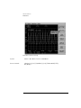
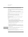
5 If you have chosen Manual to select the file name, press the Choose File to Save softkey. The
Filename Menu setup panel opens.
The Filename Menu setup panel
Entering a Filename Using the Arrow Keys
• Use the front-panel step keys (› and ?) and the arrow softkeys (Æ and ¨) to highlight each letter
2-21
Using the Instrument
Saving, Recalling, and Managing Files
of the filename.
• When the desired letter or function is selected, press the Select softkey.
• Select the BackSpace function to delete individual letters.
• Select the Clear Line function to delete the entire filename.
• When you finish entering the filename, press the SAVE FILE softkey.
Entering a Filename using an External Keyboard
There must be a PS-2 keyboard connected to the analyzer prior to bootup.
• Press [TAB] on the keyboard to highlight the entry field.
• Enter the filename using the keyboard.
• When you finish entering the filename, press the SAVE FILE softkey.
2-22
Using the Instrument
Saving, Recalling, and Managing Files
Recalling Measurement and Trace Data
You can recall measurement and trace data using the following methods:
• Fast Measurement Recall Mode
• Recall Setup Panel Mode
Refer to “Recall (Recall Setup Panel)” on page 3-61.
Recalling Data in Fast Meas Recall Mode
1 Press the front-panel Save/Recall key.
2 Press the Fast Meas RECALL softkey.
3 The instrument recalls the measurement state previously saved as FASTSAVE.dat by the Fast
Meas Save function.
Note
The auto span value will not be saved with the measurement.
Recalling Measurement and Trace Data
Note
To insure accurate measurements, a wavelength calibration should be performed each time
measurement data is recalled from memory.
1 Press the front-panel Save/Recall key.
2 Press the Recall Menu.... softkey.
3 The Recall Setup panel opens.
The Recall Menu setup panel
Note
The auto span value will not be saved with the measurement.
Recall Setup Panel
Selections
Recall
Selects whether a measurement or trace will be recalled.
2-23
Using the Instrument
Saving, Recalling, and Managing Files
Recall From
Selects whether to recall from a floppy disk or from internal memory.
4 When you are satisfied with your selections, press the Choose File to Recall softkey. The Catalog
setup panel opens.
The Catalog setup panel
5 Use the arrow keys or Prev File, Next File softkeys to highlight the desired file. Press RECALL FILE
to load the selected file.
2-24
Using the Instrument
Saving, Recalling, and Managing Files
File Sharing and Printing over a Network
This function uses the LAN to print to network printers and store, recall or delete data on remote
hard drives. The data can then to be accessed and shared among the users and printed on designated printers.
To access the file and printer share softkeys, you must first configure the network and enter the
user share identity/user profile information for remote shares. The softkeys for file and printer
share will then become available for selection.
Create a file or print share.
1 Configure the network. Refer to “Setting Up the OSA for Remote Operation” on page 4-4 for
instructions on how to configure the network.
2 From the front panel, press System > More System Functions > GPIB & Network Setup > User
Share Identity.
3 Enter the User Name, Password, and Workgroup. Use the keyboard to enter the information or
press Edit Field to access the User Workgroup Setup panel then close the panel.
4 From the Network Setup, press File Share and enter the Share Path and optional IP address. The
format of the share path is \\server\”share name.” Please note that you cannot specify directories
within the share. Up to four remote file shares are available.
5 Press Printer Shares and enter the share path and optional IP address. Use the keyboard to enter
the information or press Edit Field to access the User Workgroup Setup panel. Up to four remote
printer shares are available.
6 To activate the printer share, press System > Printer Setup and select the configured share. To
activate the file share, press Save/Recall then either Save, Recall or Delete and select the
configured share. Note if you have not configured the share the Network File Share buttons will
not be active.
2-25
Using the Instrument
Analyzing Measurement Data
Analyzing Measurement Data
This section provides advice and information on the following analyzer functions that allow you to
analyze the measured amplitude wavelength data.
• Tips for Using Traces and Markers
• Measuring the Delta between Traces
• Using Trace Math to Measure Wavelength Drift
Tips for Using Traces and Markers
The analyzer provides the ability to display up to six traces with up to four markers. Knowing a
few tips makes trace and marker manipulation much easier. Refer to “Traces” on page 3-87,
“Marker BW” on page 3-33, “Marker Search Menu” on page 3-34, “Marker Setup” on
page 3-35, and “More Marker Functions” on page 3-40.
• Markers are always placed on the currently selected active trace. Therefore, use the Active Trace
function to activate the desired trace, then select an active marker to be placed on that trace.
• When multiple markers are currently used on multiple traces, the Marker Status area (located at
the top of the display) makes it easy to identify the state of each marker.
Information provided for each marker includes:
• Wavelength
• Amplitude
• The trace associated with the marker.
For example, if marker 1 is on Trace A then the annotation will show
Mkr 1 (A).
In addition, if there are two markers on, then the delta of the wavelength and amplitude for
the two different markers is also displayed. For example, Mkr (2-1) 0.206 nm, -0.002 dB.
2-26
Using the Instrument
Analyzing Measurement Data
The color of the annotation denotes different characteristics of the markers:
• White annotation denotes the status of the currently active marker.
• Green annotation denotes the status of all currently used markers.
• Red annotation denotes that some type of an error occurred with the marker measurement.
Moving the Active Marker from One Trace to Another
The following procedure shows you how to move the active marker (marker 1) from Trace A to
Trace B.
1 From the front panel, press Markers > Active Trace > TrB to make Trace B the active trace.
2 Press Active Marker > Mkr 1.
Measuring the Difference between Traces
The following procedure shows you how to find the amplitude and wavelength difference
between the maximum peaks of two different traces. Refer to “Normal/Delta Marker Interpolation (Marker Setup Panel)” on page 3-44.
1 From the front panel, press Markers > Active Trace and select the first trace to place a marker.
2 Press Active Marker > Mkr 1 > Peak Search to place the marker on the highest peak of the active
trace.
3 Press Active Trace and select the second trace to place a marker.
4 Press Active Marker > Mkr 2 > Peak Search to place the marker on the highest peak of the second
trace.
5 View the results of the measurement from the marker annotation at the top of the display.
The wavelength and amplitude of each trace marker is shown, as well as the amplitude and
wavelength difference of the peaks of the two traces.
2-27
Using the Instrument
Analyzing Measurement Data
Using Trace Math to Measure Wavelength Drift
1 From the front panel, press Traces > Active Trace > TrA.
2 Press Single Sweep, Bandwidth Sweep, Single Sweep to update Trace A then press Traces,
Update A off.
3 Press Active Trace > TrB.
4 Press Sweep > Repeat Sweep On to continuously update the measured response on Trace B.
5 Press Traces > Trace Math, Default Math Trace C > Log Math C = A – B.
You can now monitor the wavelength drift of your device over time.
Also Refer to “Log Math C=A–B” on page 3-31, “Log Math C=A+B” on page 3-32, and “Log
Math F=C–D” on page 3-32.
2-28
Using the Instrument
Analyzer Operating Modes
Analyzer Operating Modes
This section discusses the following analyzer modes that you can use in specific measurement
applications.
• Filter Mode (For Agilent 86146B only)
• Time Resolved Chirp
Filter Mode
For Agilent 86146B only
The Agilent 86146B filter mode allows a single channel from a dense wavelength division multiplex (DWDM) signal to be isolated and routed to another measurement instrument. The filter
mode capability is built-in to internal applications to allow for fast and easy measurements. The
filtering is accurate and flexible. It has low polarization dependent loss (PDL), adjustable filter
bandwidth, and a wide tuning range.
• Switch to filter mode by pressing Appl > Measurement Modes > Filter Mode.
• Select a filter bandwidth in the BW/sweep > Res BW menu.
• Select an active tuning marker and tune it to a wavelength position.
The filter marker becomes the current marker and has the active area focus. All other markers
stay on. In the filter mode, the analyzer acts as a fixed-tuned, variable wavelength, variable
bandwidth, bandpass filter. It filters the input light at a specified wavelength. The filtered light is
available at the front-panel monochromator output connector. One application of the filter mode
is the filtering (selecting) of one particular mode of a laser source. Refer to “Filter Mode” on
page 3-26, “Filter Mode Instruction Panels” on page 3-26, and “Filter Marker Tune” on
page 3-25.
When the analyzer enters the filter mode, the sweep stops with the analyzer filter tuned to the
center wavelength. (If a marker is on, the analyzer filter is tuned to the marker wavelength.) The
last trace remains displayed to show the input spectrum before the filtering. A marker shows the
wavelength of the preselection. You can change the filtered output (preselection) wavelength by
2-29
Using the Instrument
Analyzer Operating Modes
adjusting the marker’s position, then connecting the monochromator output to another instrument. If the input spectrum changes, reconnect the monochromator output, then press the Take
Sweep softkey to capture a new sweep.
The single mode filter can be used in conjunction with the Agilent 86130A bitalyzer error performance analyzer and/or the Agilent 86100A infinium digital communication analyzer. Time
resolve chirp (TRC) measurements use the Agilent 86146B Option TRC and the Agilent 86100A
digital communication analyzer.
2-30
Using the Instrument
Analyzer Operating Modes
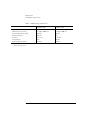
Table 2-6. Agilent 86146B unique operation
86146B Unique Operation (External 9 µm Fiber Connection)
Filter mode initialization:
• No default settings
Markers used:
• Filter marker is the normal noise marker
• OSNR marker is the center marker
• Bandwidth marker is the center wavelength marker
Functions limited to:
• Fiber selection
• Applications
• Calibration
• ADC
Filter mode functions available:
• Transfer and restore state file in filter mode
• Save in filter mode
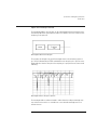
Accessing the filter mode (for 86146B only)
Note
Filter mode will not function in zero span. The filter mode selection will be shaded out. The current
state before entering filter mode will not be saved. A sweep will not be taken. The reference level
will not change.
1 Connect the light source to the optical spectrum analyzer’s front panel monochromator input
connector.
2 Connect the monochromator output to the photodetector input.
3 Press Appl’s > Measurement Modes > Filter Mode. Follow the external path align setup
instructions and select either the Switch Path Auto Align Now or Switch Path No Auto Align.
• Select the Switch Path Auto Align Now to perform an automatic alignment of the external path.
• Select Switch Path No Auto Align if you do not have the monochromator output connected to
the photodiode input, or to preserve previous align data.
2-31
Using the Instrument
Analyzer Operating Modes
Switch Path Auto Align Now switches to the 9 µm filter mode path and performs an Auto Align.
This aligns the output of the monochromator with the photodetector input for improved amplitude accuracy. The automatic alignment procedure should be performed whenever the instrument has been:
• moved
• subjected to large temperature changes
• turned off, then on, and warmed up for an hour
The automatic alignment requires the connection of an external light source. This can be a broadband or narrowband source. If there is insufficient signal power, the automatic alignment will not
be performed and an error message will be reported.
The Auto Align function saves and restores the current instrument state. This allows the auto
align to be used in the middle of a measurement routine.
If markers are turned on, auto align attempts to do the automatic alignment at the wavelength of
the active marker.
Note
Auto Align Now will overwrite any previous align data.
The data returned by the alignment is stored for both the external (9 µm) and the internal (50 µm)
path. With the data stored for both paths, the alignment for the internal path is improved due to
the increased resolution bandwidth of the external path. Once the align is complete or if you
select No Auto Align, the instrument will be ready to detect data through the external path.
4 After the routine has finished, check that the display shows the wavelength range of interest of
the external path. Adjust if necessary.
5 Press Res BW. Use the knob, step keys, or numeric keypad to enter the desired amount of
resolution bandwidth filtering.
The 9 µm optical path for filter mode uses the 0.04 nm resolution bandwidth. The resolution
bandwidths include 0.04 nm, 0.05 nm, 0.07 nm, 0.1nm, 0.2 nm, 0.3 nm, 0.5 nm, 1 nm, 2 nm, 5
nm, and 10 nm.
6 Press Take Sweep to update the display to show the results of the new resolution bandwidth
filtering.
The light is output from the optical spectrum analyzer’s front panel monochromator output connector. This light is filtered (by the resolution bandwidth) and attenuated (by the monochromator
loss) light that is input to the front panel optical input connector.
7 Press Optical Filter Marker Tune. Turn the front panel knob or press the step keys to tune the
preselector to any displayed wavelength.
8 Connect the monochromator output to an instrument.
2-32
Using the Instrument
Analyzer Operating Modes
9 If the input light changes, or if you change the span of the optical spectrum analyzer, reconnect
the monochromator output to the photodetector input, and press Take Sweep to update the
displayed trace with valid waveform data.
10 Press Exit Filter Mode to return to normal optical spectrum analyzer operation.
The filter mode Save/Recall function for the Agilent 86146B will work only in this model.
Note
If the file saved in filter mode is recalled into an instrument with firmware revision B.04.02, a
critical error occurs, indicating a grating positioning failure. Restart the instrument to clear the
error and then continue making measurements.
2-33
Using the Instrument
Analyzer Operating Modes
Time Resolved Chirp
For Agilent 86146B option DPC only
The Agilent 86146B, with the filter mode capability, will measure side mode suppression ratio
(SMSR), wavelength, and power. With the addition of an Agilent 86100 Infinium Digital Communications Analyzer (DCA), dedicated software (86146B Option TRL), and a personal computer,
time resolved chirp (TRC) of a modulated laser can be calculated.
TRC provides frequency (or wavelength) vs time information about a modulated lightwave signal.
Also called dynamic chirp, the TRC graph provides useful information on the ability of a modulated signal to propagate over long distances in optical fiber. In dense wavelength division multiplexing (DWDM) systems, excessive chirp also can cause inter-channel interference. The two
significant factors of chirp are:
• dispersion which is a function of the transmission link’s length and fiber type
• cross talk caused by chirp due to closely spaced channels
A measurement could show the modulated signal (square wave) and the chirp. The chirp fluctuates with time and the frequency change, seen at the falling and rising edge of the time domain.
The time resolved chirp solution measures:
• intensity versus time
• frequency versus time
• calculates the alpha factor
The alpha factor is also referred to as linewidth enhancement factor. One definition of a is:
a= 2P(Df) /(Dp)
During initialization, the instrument does an auto peak, gathers information about the peaks, and
tunes the filter marker. The unmodulated data in shown in the square wave pattern and the chirp
is the frequency which runs through the square wave pattern.
To smooth the chirp signal, increase the averages taken which will decrease the noise found on
the signal. Increasing the number of averages and using the longer patterns will increase the
measurement processing time. To shorten the measurement processing time, either increase the
power or decrease the number of averages. See the TRC Option User’s Guide for more details.
2-34
3
Function Reference
Function Reference
Function Reference
Function Reference
This chapter is an alphabetical reference of front panel keys, softkeys, and setup panel parameters. It is designed for quick information access. For example, during an operation you may find a
key whose function is unfamiliar to you. Note the key name and look the key up in this chapter.
Active Function Area Assist
Sets the active function area to the first or top softkey function. When this function is on, the
active area is automatically set. For example, when you press the front-panel Wavelength key,
the active function area assist will set the active function to the Center WL. You can immediately
enter the desired center wavelength without pressing the Center WL softkey. If this function is
off, the active dialog box will not appear on the display. To access the individual dialog box, press
the desired softkey function.
Key Path
System > More System Functions > Display Setup
Related Functions
Move Active Area
3-2
Function Reference
Active Marker
Active Marker
Accesses the menu that allows you to select an active marker. Selecting a marker always places
that marker on the center wavelength of the active trace. Up to four markers can be simultaneously displayed. If multiple markers are displayed, the active marker appears as a white diamond and the other markers appear as green diamonds. The Mkr notation on top of the graticule
area indicates the trace where the marker is located. For example, Marker 2 on trace B would
read Mkr 2(B).
See “Tips for Using Traces and Markers” on page 2-26, and “Measuring the Difference between
Traces” on page 2-27.
Key Path
Markers > Active Marker
Related Functions
Active Trace, Peak Search, Pit Search, Marker to Center, Marker to Reference Level
Remote Commands
CALCulate[1|2|3|4|5|6]:MARKer[1|2|3|4]:STATe
CALCulate[1|2|3|4|5|6]:MARKer[1|2|3|4]:AOFF
Active Trace
Accesses the menu that allows you to select an active trace for viewing, updating, or storing. The
trace must be active before you can put a marker on it or make changes to it. There are six traces
available.
See “Tips for Using Traces and Markers” on page 2-26, and “Measuring the Difference between
Traces” on page 2-27.
Key Path
Traces > Active Trace
Markers > Active Trace
Related Functions
Trace Math, View (Trace), Update (Trace)
Remote Commands
CALCulate[1|2|3|4|5|6]:MARKer[1|2|3|4]:TRACe
TRACe:FEED:INPute TRA,2
TRACe:FEED:CONTrol:TRA, ALWays
DISPlay:WINDow:TRACe TRA, ON
3-3
Function Reference
Adv Service Functions
Adv Service Functions
Accesses the following functions:
•
•
•
•
Key Path
Grating Order
More Adv Service Menu
Wavelength Limit
Zero Now
System > More System Functions > Service Menu > Adv Service Functions
Advanced Line Mkr Functions
Accesses the following functions:
•
•
•
•
Key Path
integrate limit
search limit
sweep limit
trace integ
Markers > More Marker Functions > Line Marker Menu > Advanced Line Mkr Functions
Agilent Logo (Display Setup Panel)
Accesses the panel that allows you to turn the Agilent logo on or off. When this function is on,
the Agilent logo appears on the display’s upper, left corner of the graticule and on printouts.
Key Path
System > More System Functions > Display Setup
All Math Off
Turns all the trace math functions off.
Key Path
Traces > Trace Math Off > All Math Off
3-4
Function Reference
All Off
All Off
Turns all the active markers off.
Note
If filter mode is on, this function is not available.
Key Path
Markers > Active Marker > All Off
Remote Commands
CALCulate[1|2|3|4|5|6]:MARKer[1|2|3|4]:AOFF
Amplitude
Accesses the menu of keys that allow you to control the instrument’s sensitivity and amplitude
scales. The function keys include:
•
•
•
•
•
•
•
Key Path
amplitude setup
display mode
peak to ref level
reference level
scale/div
sensitivity
trace integ
Amplitude
Amplitude Setup
Accesses the Amplitude Setup panel that allows you to specify amplitude related functions:
•
•
•
•
•
•
•
•
•
amplitude correction mode
amplitude correction sel
amplitude units
auto chop mode
auto ranging
auto zero
power calibration
reference level position
user power cal date
3-5
Function Reference
Amplitude Setup
The Amplitude Setup panel
Setup Panel Selections
Reference Level Position
The value selected for the Reference Level Position determines the position of the reference level
on the graticule. Setting this value to zero divisions places the reference level on the very bottom
of the grid. Setting the reference level to 10 divisions places the reference level at the top of the
grid. Pressing the front-panel Preset key resets the reference level to 9.0 divisions.
Note
When using the knob or step keys, the value will automatically change. When using the numeric
entry pad, enter a terminator that is selected from the softkey panel.
Amplitude Units
Selecting Auto for amplitude units allows power to be shown in dBm when using the logarithmic
scale, and in watts when using the linear scale. Selecting W forces the immediately displayed
information to be in watts, regardless of the amplitude scaling.
3-6
Function Reference
Amplitude Setup
Auto Ranging
The Auto Range function allows the OSA to automatically change the gain of the transimpedance
amplifier during a sweep. This allows measurements to be made at the largest dynamic range
and at the fastest sweep speed.
Pressing the front-panel Preset key turns Auto Ranging ON.
Note
It is recommended that Auto Ranging always be turned on.
Auto Zero
Turns Auto Zero ON and OFF. Auto Zero ON enables the internal amplifiers to be zeroed between
sweeps. Selecting OFF disables this feature. Pressing the front-panel Preset key resets this function to ON.
Note
Turning Auto Zero off allows the instrument to sweep faster, but results in less accuracy on low
level signals. The optical spectrum analyzer performs a more complete zeroing when the
instrument is first turned on. You can run this more complete routine anytime by pressing the Zero
Now softkey.
Auto Chop Mode
(Not available on 86146B models)
Enables the optical spectrum analyzer chop mode. Chop mode increases dynamic range for long
sweep times by subtracting ambient light. Subtracting the ambient light can improve sensitivity
but slows down the sweep speed.
Pressing the front-panel Preset key turns this function OFF.
Note
Sweep times of 50 msec × the # of trace points, or longer, use a special “chop” mode. Chop mode
increases dynamic range, stabilizes measurements against drift, and reduces effects of stray light.
This special chop mode is enabled by setting the Auto Chop mode to on.
Power Calibration
Power Calibration allows you to use amplitude correction factors either from the factory calibration or from the last successful user calibration. Pressing the front-panel Preset key resets this
function to User. If a user calibration has not been performed, the factory calibration data is used.
User Power Cal Date
The User Power Cal Date displays the date of the last successful user-performed amplitude calibration.
3-7
Function Reference
Amplitude Units (Amplitude Setup Panel)
Amplitude Correction Sel
Allows you to select a correction set to be applied to the measurement results. Only one set can
be selected at a time. Refer to “Amplitude Correction Remote Commands” on page 1-24 of the
“Agilent 8614xB Series Optical Spectrum Analyzer Programming Guide” for an
overview of the amplitude correction remote commands.
Amplitude Correction Mode
Allows you to turn the AMPCOR ON or OFF.
When AMPCOR is turned on, the correction points are applied across the active measurement
range and added to all measurement results. Between points, the correction values are interpolated linearly or logarithmically. When measuring at wavelengths outside the first and last correction points, the first or last value (as appropriate) is used as the correction value.
Whenever AMPCOR is active, the currently selected correction set is displayed in the lower left
corner of the screen. For example, if correction set number one is selected, “A1” is displayed.
Refer to “Amplitude Correction Remote Commands” on page 1-24 of the “Agilent 8614xB
Series Optical Spectrum Analyzer Programming Guide” for an overview of the amplitude correction remote commands.
Key Path
Amplitude > Amplitude Setup...
Related Functions
Reference Level, Sensitivity
Remote Commands
(Amplitude Display Mode):DISPlay:WINDow:TRACe:Y:SCALe LINear
DISPlay:WINDow:TRACe:Y:SCALe LOGarithmic
(Amplitude Units):UNIT:POWer
(Auto Zero):CALibration:ZERO
(Reference Level Position):DISPlay:WINDow:TRACe:Y:SCALe:RPOSition
Amplitude Units (Amplitude Setup Panel)
Selects the amplitude scale’s units. Selecting Auto for amplitude units allows power to be shown
in dB when using the logarithmic scale and in watts when using the linear scale. Selecting W
forces the readout to be in watts, regardless of the amplitude scaling.
Key Path
Amplitude > Amplitude Setup > Amplitude Units
Related Functions
Display Mode, Trace Marker, Scale/Div
3-8
Function Reference
Auto Align
Remote Commands
UNIT:POWer
Auto Align
Pressing the auto align button on the front panel of the instrument performs an automatic alignment of the instrument using the largest signal found in a full span sweep. This aligns the output
of the monochromator with the photodetector for improved amplitude accuracy. To ensure maximum amplitude accuracy and stability, connect an input signal to the instrument, mark the peak
of the signal, and then press Auto Align. This starts an automatic alignment procedure that
should be performed whenever the instrument has been:
• moved
• subjected to a 2° temperature change
• restarted and warmed up at the start of each day
The automatic alignment requires the connection of an external, broadband or narrowband, light
source. If there is insufficient signal power, the automatic alignment will not be performed and an
error message will be reported.
The auto align function saves and restores the current instrument state. This allows the auto align
function to be used in the middle of a measurement routine.
If markers are turned on, the auto align function attempts to do the automatic alignment at the
wavelength of the active marker. If the instrument is in zero span, the alignment is performed at
the center wavelength.
Key Path
Auto Align
Related Functions
Auto Meas
Auto Align & Add to Trajectory
Calibrator Multi-Pt Align
User Source Multi-Pt Align
Remote Commands
CALibration:ALIGn
CALibration:ALIGn:MARKer[1|2|3|4]
3-9
Function Reference
Auto Align & Add to Trajectory
Auto Align & Add to Trajectory
Allows alignment at several wavelengths, ensuring amplitude accuracy of your measurements.
Before initiating the alignment, connect a broadband light source to the front-panel input connector. (You may add and/or update the existing points in the trajectory table.) Press Auto Align
Preset to clear the table.
Turn on an active marker and manually place the marker at the desired wavelength. If an active
marker is not turned on, the instrument will automatically turn on an active marker and auto align
at the largest input signal. The minimum recommended spacing between points is 5 nm for the
external, single mode fiber (Agilent 86146B only) and 50 µm for the internal, multi-mode fiber.
The span must be >3 nm for the single mode fiber and >25 nm for the multi-mode fiber.
Note
Error 5001, Auto align cannot find input signal, will occur if a broadband light source is not
connected to the front-panel input connector.
Error 5070, Trajectory Add Failed, will occur if the trajectory table is full or the computed trajectory
table is invalid.
Key Path
Systems > More System Functions > Service Menu > Adv Service Functions >More Adv Service Menu > Multi-Point Align > Auto Align & Add to Trajectory
Related Functions
Auto Align Preset
Calibrator Multi-Pt Align
User Source Mutli-Pt Align
Remote Commands
CALibration:ALIGn:TADD
Auto Meas
Pressing the Auto Meas button on the front panel of the instrument performs an automatic measurement of the largest signal found in a full span sweep and places a marker at the signal peak.
The signal must have at least 10 dB of excursion. (Refer to “Peak Excursion (Marker Setup
Panel)” on page 3-51 for additional information.) Auto measure requires the connection of an
external, broadband or narrowband light source. If there is insufficient signal power, the automatic measurement will not be performed, and a warning message will be reported. This automatic measurement routine is normally the best way to adjust sensitivity while maintaining the
fastest sweep rates.
3-10
Function Reference
Auto Meas
The auto measure function uses trace A to perform the measurement. Since the auto measure
function can alter the instrument state, we recommend that this operation be performed before a
measurement sequence is started.
Auto Measure Setup panel allows you to modify the auto measure span and the vertical scale,
tune to the wavelength indicated by the marker, and optimize the sensitivity.
Span selects the wavelength span for viewing the signal located by the auto measure function. If
auto is specified, the span is set wide enough to display most of the signal. If a particular span is
desired, deselect auto and put the desired span in the nm dialog box. The default selection for
span is auto.
Note
If the span is set too narrow, the auto measure operation may not complete successfully. If this
happens a warning message is displayed.
Scale/Div selection sets the vertical scale to be used after performing the auto measure function.
If auto is specified, the measurement function sets the vertical scale to a value based on the
dynamic range of the signal. If a particular vertical scale is desired, deselect auto and put the
desired dB/div in the dB dialog box. The default selection for dB/div is auto.
AutoMeas at Marker turns the auto measure marker on or off. Selecting the on state for auto
measure at marker causes the auto measure function to perform its operation at the wavelength
of the active marker. This allows you to measure a signal other than the largest one found in a full
span sweep. The default selection for auto measure at marker is off.
Optimize Sensitivity, when turned on, causes the auto measure function to set the sensitivity so
the resulting measurement has a minimal amount of noise. It does this by finding the minimum in
the measurement trace and comparing this value to the known sensitivity of the instrument at
that wavelength. Sensitivity is then reduced until the signal is close to this minimum sensitivity or
the sweep time becomes too long. The Optimize Sensitivity function is useful when viewing high
dynamic range signals. The drawback to turning this function ON is that it generally requires a
longer sweep time to get better sensitivity. The default selection for Optimize Sensitivity is OFF.
Note
None of the Automeasure Setup parameters are affected by the front-panel Preset key. They are
not saved as part of the measurement setup.
Key Path
Auto Meas
Related Functions
Auto Align
Remote Commands
DISPlay[:WINDow[1]]:TRACe:ALL[:SCALe][:AUTO]
DISPlay[:WINDow[1]]:TRACe:X{:SCALe]:AUTO:SPAN
DISPlay[:WINDow[1]]:TRACe:Y{:SCALe]:AUTO:PDIVision
DISPlay[:WINDow[1]]:TRACe:ALL[:SCALe][:AUTO]:MARKer OFF|ON|0|1
3-11
Function Reference
Auto Ranging (Amplitude Setup Panel)
Auto Ranging (Amplitude Setup Panel)
When on, the auto ranging allows the OSA to achieve the desired sensitivity by taking several
sweeps and switching between gain stages. The final trace data is a blended composite of each
trace taken in the different gain stages.
Note
The sweep time (ST) that is displayed in the lower portion of the display is the time that it takes
for the OSA to sweep over one gain stage. The OSA may take up to three sweeps in three different
gain stages to make the measurement. This depends on the settings for sensitivity, reference level,
auto range and also the particular device being measured. The final data trace is a blended
composite of each trace taken in the different gain stages. For more information, refer to “Sweep
Time” on page 3-81.
Setting Auto Range to off will force the OSA to use a single gain stage and achieve the desired
sensitivity by applying a digital filter.
Key Path
Amplitude > Amplitude Setup > Auto Range
Remote Commands
SENSe:POWer:DC:RANGe:AUTO
Auto Zero (Amplitude Setup Panel)
Turns Auto Zero on and off. Auto Zero on enables the internal amplifiers to be zeroed between
sweeps. In this mode, the instrument compensates for temperature-related current drift between
each sweep. Although this “zeroing” increases amplitude accuracy, it also increases the time
between sweeps. If amplitude accuracy is not critical to your measurement, turning off auto zero
will improve throughput. Pressing the front-panel Preset key resets this function to on.
Tip: The instrument performs a more complete zeroing when the instrument is first turned on. You
can run this more complete routine anytime by pressing the Zero Now (System > More System
Functions > Service Menu > Adv Service Functions > Zero Now) softkey.
Key Path
Amplitude > Amplitude Setup > Auto Zero
Related Functions
Zero Now
Remote Commands
CALibration:ZERO
3-12
Function Reference
Averaging
Averaging
When averaging is on, you can select the number of measurement sweeps to be averaged, using
the 10, 20, 50, 100 softkeys. You can also enter averaging values other than those displayed by
using the numeric keypad or the knob.
When the number of sweeps taken is less than the count, the following formula is used to calculate the data:
AVG = sum of current sweeps/ number of averages selected
If the number of sweeps is greater than or equal to the count, the following formula is used to
calculate the data:
New average = [(count-1)/count] x last average + new measurement/count
Key Path
Traces > Averaging
Remote Commands
CALCulate[1|2|3|4|5|6]:AVERage:COUNt
CALCulate[1|2|3|4|5|6]:AVERage:STATe
Backup Internal Memory
Allows you to make a complete backup of user memory onto a floppy disk. All user files (measurement, trace, and specification sets) are saved. You can recall the backup contents into the
instrument with the Restore Internal Memory function. Refer to “Backing Up or Restoring the
Internal Memory” on page 2-19
A screen appears asking you to insert a formatted floppy disk into the floppy drive. The disk will
not be viewable on a PC and no trace or measurement files can be saved onto the disk until it is
reformatted. The backup internal memory function overwrites the floppy disk with a new image,
so only the latest backup information can be recovered through the Restore Internal Memory
operation. Any existing files or catalogs on the floppy disk will be destroyed.
Key Path
Save/Recall > Backup/Restore Menu > Backup Internal Memory
3-13
Function Reference
Backup/Restore Menu
Backup/Restore Menu
Accesses the instrument utilities used to backup or restore internal memory.
Key Path
Save/Recall > Backup/Restore Menu
3-14
Function Reference
Bandwidth Marker Interpolation (Marker Setup Panel)
Bandwidth Marker Interpolation (Marker Setup Panel)
Turns the bandwidth marker interpolation on or off. When on, the bandwidth markers will be
placed at the exact number of dB (NDB) from the normal marker, if within the trace range. The
position of the marker will be linearly interpolated between the two nearest trace data points.
The default state is on. If interpolate is off, for negative number of dB (NDB) values, the bandwidth markers will be at values closest to and more negative then the NDB value. For positive
NDB values, the bandwidth markers will be at values closest to and more positive than the NDB
values. This will typically result in a wider bandwidth measurement.
Key Path
Markers > Marker Setup > Bandwidth Marker Interpolation
Related Functions
Active Marker, Delta Marker, Bandwidth Marker
Remote Commands
CALCulate[1|2|3|4|5|6]:MARKer[1|2|3|4]:FUNCtion:BANDwidth
:INTerpolation
Bandwidth/Sweep
Accesses the menu that allows you to change bandwidth, sweep settings, fiber selection, trigger
mode, and ADC sync. You can also access these functions from the Measure menu Bandwidth/
Sweep selection. The function keys include:
•
•
•
•
•
•
•
more BW/sweep functions
repeat sweep
res BW
select fiber
single sweep
sweep time
video BW
BW Marker Units (Marker Setup Panel)
Sets the bandwidth marker X-axis readout for frequency or wavelength when the instrument is in
a non-zero span. The available selections are nm, µm, Ang, GHz, and THz. The default unit is nm
(nanometers). This setting controls all four bandwidth markers. The normal and delta offset markers have their own settings.
3-15
Function Reference
Calibration
Key Path
Markers > Marker Setup > BW Marker Units
Related Functions
Marker BW
Remote Commands
CALCulate[1|2|3|4|5|6]:MARKer[1|2|3|4]:FUNCtion:BANDwidth:READout
Calibration
Accesses the Power Cal Setup and Wavelength Calibration Setup softkeys. The Power Calibration Setup panel will show the date of the last factory performed power calibration and the date
of the last successful user-performed power calibration. It also allows you to set the calibration
power and wavelength used for the next calibration. Refer to “Calibrating Wavelength Measurements” on page 2-13
Set Calibration Power is the exact amplitude of the calibration source that will be used for the
next power calibration. The power entered must be within +10 dBm and –3 dBm of the amplitude measured using the factory calibration.
Set Calibration Wavelength is the approximate wavelength of the calibration source that will be
used for the next user power calibration. The wavelength entered must be within 2.5 nm of the
wavelength measured using the factory calibration.
Pressing the Perform Calibration softkey will display on-screen instructions for performing the calibration.
Key Path
Systems > Calibration
Remote Commands
CALibration:POWer:POWer
CALibration:POWer:Wavelength
Calibrator Multi-Pt Align
Adjusts the mechanical position of the instrument’s internal optical components ensuring amplitude accuracy of your measurements. Before initiating the alignment, connect the internal calibrator to the front-panel input connector. Refer to “External Multipoint Wavelength Calibration”
on page 2-16
3-16
Function Reference
Center Wavelength (WL)
The instrument automatically sets the start wavelength at 1490 nm, stop wavelength at 1590
nm, span, and reference level, and then performs a fully automatic, internal auto align. The input
signal is aligned at equally spaced alignments (minimum 50 nm spacing between points) for the
internal, multi-mode fiber or (minimum 5 nm spacing between points) for the external, singlemode fiber (Agilent 86146B only).
Note
Error 5056, Trajectory align cannot find input signal, will occur if a broadband light source is not
connected to the front-panel input connector.
Error 5060, Trajectory align failed, will occur if the align procedure failed.
Key Path
System > More System Functions > Service Menus > Adv Service Functions > More Adv Service Menu > Multi-Point Align > Calibrator Multi-Pt Align
Related Functions
Auto Align & Add To Trajectory
Auto Align Preset
User Source Multi-Pt Align
Remote Commands
CALibration:ALIGn:INTernal
Center Wavelength (WL)
Sets the center wavelength using the knob, step keys, or numeric keys. The span remains constant. The center wavelength and the start and stop wavelength settings are related as follows:
Center Wavelength = (stop wavelength + start wavelength)/2
Key Path
Wavelength > Center WL
Related Functions
Start WL, Stop WL, Span
Remote Commands
SENSe:WAVelength:CENTer
3-17
Function Reference
Center Wavelength Step Size (Wavelength Setup Panel)
Center Wavelength Step Size (Wavelength Setup Panel)
Specifies the center wavelength step size. This is used for incrementing center wavelength using
the ¦ and Ø keys.
Key Path
Wavelength > Wavelength Setup > Center Wavelength Step Size
Remote Commands
SENSe:WAVelength:CENTer:STEP:INCRement
Configure Network
Starts a utility that allows you to enable and configure networking. Enter this menu only if you
have all the necessary networking parameters. Refer to “File Sharing and Printing over a Network” on page 2-25
Key Path
System > More System Functions > GPIB & Network Setup > Configure Network
Current GPIB Address (Remote Setup Panel)
Displays the GPIB address currently being used. To change the address, use the numeric keys,
step keys, or knob to enter the new GPIB address information in the Remote Setup panel.
Key Path
System > More System Functions > GPIB & Network Setup > GPIB Address
Current Source Setup
Accesses the Current Source Setup panel that allows you to turn on or off the current source, set
the current limit, enable pulse width, duty ratio, and synchronize the ADC sync output. Refer to
“Operating the Internal White Light Source” on page 2-4
Key Path
System > Options > Current Source Setup
Related Functions
ADC sync, current limit, pulse width, duty ratio
3-18
Function Reference
Date/Time (Display Setup Panel)
Remote Commands
SOURce:CURRent:PULSe:STATe ON|OFF
Date/Time (Display Setup Panel)
Turns the date and time on the display on or off. When on, the date and time will appear on the
display’s lower, right corner of the display and on printouts.
Key Path
System > More System Functions > Display Setup
Related Functions
SYSTem:TIMe
Default Math Trace C
Defines the math expression to be used and turns the math operation on: C=ALOG-B, C=ALOG+B,
C=ALIN-B, or C=ALIN+B. The result is placed in Trace C. The math operation is performed in linear
units.
See “Using Trace Math to Measure Wavelength Drift” on page 2-28.
Key Path
Traces > Trace Math Off > Default Math Trace C
Remote Commands
CALCulate3:MATH:STATE OFF|ON|0|1
Default Math Trace F
Defines the math expression to be used and turns the math operation on: F=CLOG-D. The result is
placed in Trace F. The math operation is performed in linear units.
See “Using Trace Math to Measure Wavelength Drift” on page 2-28.
Key Path
Traces > Trace Math Off > Default Math Trace F
Remote Commands
CALCulate6:MATH:STATE OFF|ON|0|1
3-19
Function Reference
Delete From (Delete Setup Panel)
Delete From (Delete Setup Panel)
Selects whether to delete a file from a floppy disk, internal memory, or a networked file share.
Key Path
Save/Recall > Delete Menu > Delete File From
Remote Commands
MMEMory:DELete
Delete Menu
Accesses the Delete Setup panel that allows you to delete files from a floppy disk, internal memory, or a networked file share.
Key Path
Save/Recall > Delete Menu
Remote Commands
MMEMory:DELete
Delta Marker On/Off
This toggle function fixes the position of the reference marker and activates the delta marker. This
measures the difference between the active (reference) marker and the delta marker. The front
knob, step keys, or keypad can be used to move the delta marker to the desired location. Refer to
“Measuring the Difference between Traces” on page 2-27
If the delta function is turned on and no marker is active, Marker #1 will be turned on and placed
at the center wavelength as a reference for the delta marker.
Note
For Agilent 86146B only, if filter mode is enabled, the noise marker, delta marker, and OSNR
marker are disabled.
Key Path
Markers > More Marker Functions > Delta Marker
Remote Commands
CALCulate[1|2|3|4|5|6]:MARKer[1|2|3|4]:FUNCtion:DELTa:STATe
3-20
Function Reference
Delta Marker Units (Marker Setup Panel)
Delta Marker Units (Marker Setup Panel)
Sets the delta marker X-axis readout for frequency or wavelength when the instrument is in a
non-zero span. The available selections are nm, µm, Ang, GHz, and THz. The default units are nm
(nanometers). This setting controls all four delta markers. The normal and bandwidth markers
have their own settings.
Key Path
Markers > Marker Setup > Delta Marker Units
Related Functions
Delta Marker
Remote Commands
CALCulate[1|2|3|4|5|6]:MARKer[1|2|3|4]:FUNCtion:DELTa:X:READout
Display Mode
Accesses the choice of log (logarithmic) or lin (linear) data display.
Key Path
Amplitude > Display mode
Remote Commands
DISPlay:WINDow:TRACe:Y:SCALe:SPACing LINear|LOGarithmic
Display Setup
Accesses the display setup panel selections which include:
•
•
•
•
•
•
active function area assist
Agilent logo
date/time
filter mode instrument panels
path change instrument panel
title
3-21
Function Reference
Display Setup
The Display Setup panel
Setup panel selections
Agilent Logo
When this function is ON, the Agilent logo is shown on the display and printouts.
Date/Time
Turns the date and time ON or OFF on the display.
Title
Turns the title ON or OFF on the display.
Active Function Area Assist
Automatically sets the Active Function Area (when function is turned on) to the first or top softkey. For example, when you press the front-panel Bandwidth/Sweep key, the Active Function
Area Assist function will set the Active Function Area to resolution bandwidth. This means you
can immediately enter the desired resolution bandwidth. There is no need to press the Res BW
softkey
Path Change Instructions Panels
For the Agilent 86146B Filter Mode only
Allows the choice of disabling the external path align setup instructions.
Filter Mode instruction Panels
For the Agilent 86146B Filter Mode only
Allows the choice of disabling the auto align, auto measure, and take sweep setup instructions.
Key Path
System > More System Functions > Display Setup
Remote Commands
DISPlay:WINDow:TEXT:DATA <string>
3-22
Function Reference
Exchange Menu
Exchange Menu
Accesses the trace exchange selections which include:
•
•
•
•
•
•
A Exchange B
B Exchange C
C Exchange A
D Exchange A
E Exchange A
F Exchange A
Exchanges the X- and Y-axis data of the two traces. The trace pairs that can be exchanged are
Trace A with any trace, and Trace B with Trace C.
Key Path
Traces > Trace Math > Exchange Menu
Remote Commands
TRACe:EXCHange
Factory Preset (IP)
Performs an instrument preset and clears user settings that are not affected by Preset. That is,
alignment settings, user calibration, multipoint amplitude correction data. User trace and measurement files will be maintained. See “Preset” on page 3-59.
Key Path
System > More System Functions > Service Menu > Factory Preset (IP)
Related Functions
Preset
Remote Commands
CALibration:ALIGn:PRESet
Fast Meas Recall
Accesses the fast measure recall function that recalls the measurement state previously saved as
FASTSAVE.dat in the internal memory by the Fast Measure Save function. Refer to “Recalling
Data in Fast Meas Recall Mode” on page 2-23
3-23
Function Reference
Fast Meas Save
Key Path
Save/Recall > Fast Meas Recall
Related Functions
Recall, Fast Meas Save
Fast Meas Save
Accesses the fast measure save function to save the current measurement state to internal memory as FASTSAVE.dat. Allows a quick save of the current state, which can then be recovered by
the Fast Meas Recall function. Only one FASTSAVE.dat file exists, so performing a Fast Meas
Save will overwrite any currently existing Fast Save file. Refer to “Saving Data in Fast Meas Save
Mode” on page 2-19
Key Path
Save/Recall > Fast Meas Save
Related Functions
Save, Fast Meas Recall
File Name (Save Setup Panel)
Selects automatic or manual mode for saving a filename.
When Auto is selected, the measurement is automatically named and saved to an auto generated filename when the Auto Save softkey is pressed. Measurement data is saved to the filename ST_xxxxx.dat and Trace(s) only is saved to the filename TR_xxxxx.csv. “xxxxx” represents a
numbering system which is incremented each time the measurement data is saved. For example,
the first time you save Trace(s) only data, the filename TR_00001.csv will be assigned.
When Manual is selected, pressing the Choose File to Save softkey will access the Filename
Menu setup panel. Use the front panel step keys, knob, or arrow softkeys to highlight and then
select each letter in the filename. Filenames can also be set with an external keyboard, Refer to
“Entering a Filename using an External Keyboard” on page 2-22. When you finish entering the
filename, press SAVE FILE.
Key Path
Save/Recall > Save Menu > File Name
Remote Commands
*SAV
3-24
Function Reference
File Shares
File Shares
Uses the LAN (local area network) to store, recall, and delete files on remote hard drives. The
data can then be accessed and shared among the users.
To access the file and printer share softkeys, you must first configure the network refer to “Connecting to the OSA over the Network” on page 4-6 and enter the user share identity/user profile
information for remote shares (refer to “File Sharing and Printing over a Network” on page
2-25). The softkeys for file and printer share will then become available for selection.
Note
Samba® or Microsoft® software must be installed to run the file share programs.
Note
If networking is not configured, the command will generate a “Settings conflict” error.
Key Path
Systems > More System Functions > GPIB & Network Setup > File Shares
Related Commands
Printer Share
Remote Commands
SYSTem:COMMunicate:NETWork:USERname <param>
SYSTem:COMMunicate:NETWork:PASSword <param>
SYSTem:COMMunicate:NETWork:WORKgroup <param>
Filter Marker Tune
For Agilent 86146B Filter Mode only.
Tunes the wavelength of the preselector. During the preselector instrument mode, the instrument
acts as an optical filter at a fixed wavelength. Although the instrument is not sweeping the displayed input range, the last sweep remains displaying the input spectrum. With filter marker tune
softkey selected, use the front panel knob, step keys, or numeric keypad to change the preselector wavelength. Press Take Sweep to update the displayed response at any time.
The amount of filtering is determined by the resolution bandwidth setting. Narrower resolution
bandwidth settings will filter the signal more. If the resolution bandwidth is changed, Filter
Marker Tune must be reselected to tune the monochromator. Marker movement will not tune the
monochromator unless Marker Tune is active.
The front panel, single mode preselector monochromator connector allows the channel drop
capability to the Agilent 86130A BitAlyzer error performance analyzer or the Agilent 86100A
Infinium digital communication analyzer.
3-25
Function Reference
Filter Mode
Note
During filter mode, the noise marker, delta marker, and OSNR marker are disabled.
Key Path
Appl’s > Measurement Modes > Filter Mode > Switch Path Auto Align Now or Switch Path
No Auto Align > Filter Marker Tune
Remote Commands
CALCulate[1|2|3|4|5|6]:MARKer:SRLevel
INPut:FILTer:SCENt
INPut:FILTer:SRLevel
Filter Mode
For the Agilent 86146B Filter Mode only.
The filter mode utilizes the 9 µm external optical path to increase dynamic range and resolution
bandwidth with the Agilent 86146B filter mode. An active tuning marker can be selected and
tuned to the wavelength position. The filter marker becomes the current marker and has the
active area focus. All other markers stay on. Refer to “Analyzing Measurement Data” on
page 2-26 for further information. Also see “Time Resolved Chirp” on page 2-34
Key Path
Appl’s > Measurement Modes > Filter Mode
Remote Commands
INSTrument:SELect “FILTER”
Filter Mode Instruction Panels
For the Agilent 86146B Filter Mode only
Allows the choice of disabling the auto align, auto measure, and take sweep setup instructions
when switching from internal to external path.
Key Path
System > More System Functions > Display Setup > Filter Mode Instrument Panels
3-26
Function Reference
Firmware Upgrade
Firmware Upgrade
The instrument will restart into a utility to upgrade the instrument firmware. For upgrade instructions, or to order a firmware upgrade kit, visit or web site at http://www.agilent.com/comms/
osaupgrade
Key Path
System > More System Functions > Service Menu > Firmware Upgrade
Format Floppy Disk
Formats a 3.5, 1.44 MB floppy disk. The instrument does not support formatting 2.0 MB floppy
disks. Refer to “Saving, Recalling, and Managing Files” on page 2-18
3-27
Function Reference
GPIB Address
Key Path
Save/Recall > Format Floppy Disk
GPIB Address
Accesses the GPIB address information. To change the address, use the numerical entry keys,
step keys, or knob to enter the new GPIB address information. If changes are made, press the
Select softkey. Press the Defaults softkey to reset the address to the factory preset default, 23.
Key Path
System > More System Functions > GPIB Address & Network Setup > GPIB Address
GPIB & Network Setup
Accesses the functions used to set up networked file and printer shares on the analyzer.
•
•
•
•
•
Key Path
GPIB Address
Configure Network
User Share Identity
File Shares
Printer Shares
System> More System Functions > GPIB Address & Network Setup
Help
Accesses error queues for: hardware errors, critical errors, notices, and warnings once an error
queue is accessed. Also displays the instrument’s current firmware revision. Refer to “Firmware
Upgrade” on page 3-27You can print the queue, clear the queue, or page up and down to view
the information. If no hardware errors, critical errors, notices, or warnings have been generated,
these functions will be shaded.
Key Path
System > Help
Remote Commands
SYSTem:ERRor?
*IDN?
3-28
Function Reference
Hold A...F None Min Max (trace)
Hold A...F None Min Max (trace)
Hold Max compares the current amplitude value of each point on the active trace in the current
sweep to the corresponding point detected during the previous sweep, then displays the maximum value.
Hold Min compares the current amplitude value of each point on a trace in the current sweep to
the corresponding point detected during the previous sweep, then displays the minimum value.
Hold None turns the Hold function off.
Key Path
Traces > Hold None Min Max
Remote Commands
CALCulate[1|2|3|4|5|6]:MAXimum:STATe
CALCulate[1|2|3|4|5|6]:MINimum:STATe
Integrate Limit
Calculates the power between Wavelength Marker 1 and Wavelength Marker 2 when the trace
integration function is on.
Once wavelength markers have been turned on, the total power integration marker search, and
wavelength sweep may be individually limited to the wavelength marker range.
Key Path
Markers > More Marker Functions > Line Marker Menu > Advanced Line Mkr Functions >
Integrate Limit
Related Functions
Sweep Limit, Search Limit
Remote Commands
CALCulate:TPOWer:IRANge:LOWer
CALCulate:TPOWer:IRANge:UPPer
Light Source
Turns the desired light source on or off. The number and type of sources displayed depends on
the options installed. Refer to “Operating the Internal White Light Source” on page 2-4
3-29
Function Reference
Line Marker Menu
Key Path
System > Options > Light Source
Related Functions
Current Source Setup
Remote Commands
SOURce:CATalog
SOURce:STATe
Line Marker Menu
Accesses the following line marker functions:
•
•
•
•
Key Path
Advanced Line Mkr Functions
Line Markers Off
Wavelength Line Mkr 1
Wavelength Line Mkr 2
Markers > More Marker Functions > Line Marker Menu
Line Markers Off
Turns off all line markers and line marker functions.
Key Path
Markers > More Marker Functions > Line Marker Menu > Line Markers Off
Remote Commands
CALCulate[1|2|3|4|5|6]:MARKer[1|2|3|4]:SRANge:OFF
Lin Math C=A–B
Subtracts Trace B from Trace A point by point, then stores the results in Trace C in linear units. If
Trace A is in View On mode, this function is continuous and occurs every sweep. Results of the
subtraction are referenced to 0 dB. This often requires a reference level adjustment. For example, if the reference level is set at –40 dBm, Trace A is at –50 dBm, and Trace B is at –55 dBm,
the C=A–B function places Trace C at –5 dB. Because this is off screen, the reference level will
need to be adjusted.
3-30
Function Reference
Lin Math C=A+B
Key Path
Traces > Trace Math OFF > Default Math Trace C > Lin Math C=A–B
Remote Commands
CALCulate3:MATH:EXPRession(TRA–TRB)
Lin Math C=A+B
Adds Trace A and Trace B point by point, then stores the results in Trace C in linear units. The
results of this function often require a reference level adjustment. Trace A is placed in View On
mode. Trace math is mainly used to normalize the display during stimulus-response measurements.
Key Path
Traces > Trace Math OFF > Default Math Trace C > Lin Math C=A+B
Remote Commands
CALCulate3:MATH:EXPRession(TRA+TRB)
Local
Restores front-panel control of the instrument. Whenever the instrument is in Remote mode, the
RMT message is displayed on the instrument’s screen and all keys are disabled except for the
front-panel Local key.
Key Path
Local
Remote Commands
GPIB GoTo Local Command
Log Math C=A–B
Subtracts Trace B from Trace A point by point, then stores the results in Trace C in logarithmic
units. If Trace A is in View On mode, this function is continuous and occurs every sweep. Results
of the subtraction are referenced to 0 dB. This often requires a reference level adjustment. For
example, if the reference level is set at –40 dBm, Trace A is at –50 dBm, and Trace B is at –55
dBm, the C=A–B function places Trace C at –5 dB. Because this is off screen, the reference level
will need to be adjusted.
Key Path
Traces > Trace Math OFF > Default Math Trace C > Log Math C=A–B
3-31
Function Reference
Log Math C=A+B
Related Functions
Log Math C=A+B, Log Math F=C–D
Remote Commands
CALCulate3:MATH:EXPRession(TRA/TRB)
Log Math C=A+B
Adds Trace A and Trace B point by point, then stores the results in Trace C in logarithmic units.
The results of this function often require a reference level adjustment. Trace A is placed in View
On mode. Trace math is mainly used to normalize the display during stimulus-response measurements.
Key Path
Traces > Trace Math OFF > Default Math Trace C > Log Math C=A+B
Related Functions
Log Math C=A–B, Log Math F=C–D
Remote Commands
CALCulate3:MATH:EXPRession(TRA*TRB)
Log Math F=C–D
Subtracts Trace D from Trace C point by point, then stores the results in Trace F in logarithmic
units. If Trace C is in View On mode, this function is continuous and occurs every sweep. Results
of the subtraction are referenced to 0 dB. This often requires a reference level adjustment. For
example, if the reference level is set at –40 dBm, Trace D is at –50 dBm, and Trace C is at
–55 dBm, the F=C–D function places Trace F at –5 dB. Because this is off screen, the reference
level will need to be adjusted.
Key Path
Traces > Trace Math OFF > Default Math Trace F > Log Math F=C–D
Related Functions
Log Math C=A–B, Log Math C=A+B
Remote Commands
CALCulate6:MATH:EXPRession(TRC/TRD)
3-32
Function Reference
Marker BW
Marker BW
Measures the passband of the signal. To enter the bandwidth amplitude of the bandwidth markers, make a selection from the softkeys
(–3 dB, –6 dB, –10 dB, and –20 dB) or use the knob, step keys, or numeric keys. Marker bandwidth information is displayed at the top of the graticule.
If a peak search is not performed, then pressing Marker BW finds the bandwidth around the currently active marker. If the bandwidth markers cannot be placed at the selected value, an error
message, such as “BW not found” will be displayed.
See “Using Span to Zoom In” on page 2-7.
Key Path
Markers > More Marker Functions > Marker BW
Related Functions
Peak Search
Remote Commands
CALCulate[1|2|3|4|5|6]:MARKer[1|2|3|4]:FUNCtion:BANDwidth:STATe
CALCulate[1|2|3|4|5|6]:MARKer[1|2|3|4]:FUNCtion:BANDwidth:INTerpolate
(-0.5 dB|-3 dB|-6 dB|-10 dB|-20 dB)
CALCulate[1|2|3|4|5|6]:MARKer[1|2|3|4]:FUNCtion:BWIDwidth:NDB
CALCulate[1|2|3|4|5|6]:MARKer[1|2|3|4]:FUNCtion:BANDwidth:RESult?
Marker Off
Turns the current active marker off.
Key Path
Markers >Active Marker > Marker Off
Remote Commands
CALCulate[1|2|3|4|5|6]:MARKer[1|2|3|4]:STATe OFF
CALCulate[1|2|3|4|5|6]:MARKer[1|2|3|4]:AOFF
3-33
Function Reference
Marker Search Menu
Marker Search Menu
Accesses the following marker peak and pit search functions:
•
•
•
•
•
peak or pit search mode
peak or pit search
next peak down, left or right
next pit up, left or right
active markers
The active markers can also be turned on or off from this menu, which avoids returning to the
Marker menu to change markers.
Key Path
Markers > More Marker Functions > Marker Search Menu
Marker Search Threshold Value (Marker Setup Panel)
Sets the amplitude threshold value used for limiting the marker search function. Any peaks below
the threshold value will be ignored. When the Marker Search Threshold is on, a dotted line is
shown on the display at the threshold level. The Use Marker Search Threshold function in the
Marker Setup Panel must be enabled or the Marker Search Threshold Value will be greyed out.
Key Path
Markers > Marker Setup > Marker Search Threshold Value
Related Functions
Pit Excursion, Peak Excursion, Marker Search Threshold
Remote Commands
CALCulate:THReshold
CALCulate:THReshold:STATe
3-34
Function Reference
Marker Setup
Marker Setup
Accesses a menu that allows you to make changes to default marker settings. From the setup
panel you can make changes to:
•
•
•
•
•
•
•
•
•
•
•
•
Bandwidth/Marker Interpolation On|Off
BW Marker Units
Delta Marker Units
Marker Search Threshold Value
Noise Marker Reference Bandwidth
Normal/Delta Marker Interpolation On|Off
Normal Marker Units
OSNR Noise
Peak Excursion
Peak Search at End of Each Sweep On|Off
Pit Excursion
Use Marker Search Threshold
The Marker Setup panel
3-35
Function Reference
Marker Setup
Setup Panel Selections
Normal Marker Units
Sets the X-axis immediately displayed marker information for frequency or wavelength when the
instrument is in a non-zero span. This setting controls only the normal marker X-axis and the delta
reference immediately displayed information. This setting controls all four normal markers. The
bandwidth and delta offset markers have their own settings.
BW Marker Units
Sets the bandwidth marker X-axis immediately displayed information for frequency or wavelength when the instrument is in a non-zero span. The delta markers have their own setting. This
setting controls all four bandwidth markers.
Delta Marker Units
Sets the delta marker X-axis immediately displayed information for frequency or wavelength
when the instrument is in a non-zero span. The bandwidth markers have their own setting. This
setting controls all four delta markers.
Normal/Delta Marker Interpolation
Turns the normal/delta marker interpolation on or off. When interpolation is ON, the normal/delta
markers will be placed at the exact wavelength or frequency value selected if it is within the trace
range. The marker will linearly interpolate between two trace data points. The default state is off.
This setting controls the interpolation state for all four markers when in the normal or delta mode.
When interpolation is off, the marker will be placed at the trace point nearest the requested
value.
Bandwidth Marker Interpolation
Turns the bandwidth marker interpolation on or off. When interpolation is ON, the bandwidth
markers will be placed at the exact number of dB (NDB) from the normal marker if within the
trace range. The position of the marker will be linearly interpolated between two trace data
points. The default state is ON. If interpolate is OFF, for negative NDB values, the bandwidth markers will be at values closest to and more negative than the NDB value. For positive NDB values,
the bandwidth markers will be at values closest to and more positive than the NDB values. This
will typically result in a wider bandwidth measurement.
3-36
Function Reference
Marker Setup
Peak Excursion
Determines (in dB) which side modes are included in the measurements. To be accepted, each
trace peak must rise, and then fall, by at least the peak excursion value about a given spectral
component. The default value is 3 dB. Setting the value too high may result in not identifying a
side mode. Setting the value too low may cause unwanted responses, including noise spikes, to
be identified. Use the Marker Setup panel to change the peak excursion value.
Peak excursion criteria
Changing the peak excursion. The peak searches may not recognize valid signals near the noise
floor when the peak excursion definition is less than 3 dB. Thus, before performing peak searches
on signals near the noise floor, reduce the peak excursion value. However, reducing the excursion value often causes peak searches to identify noise spikes. To avoid this misidentification, use
video averaging or video filtering to reduce the noise floor variance to a value less than the peak
excursion definition.
Pit Excursion
Sets the pit excursion value for the marker search routines.
Pit excursion criteria
The pit excursion value is used to determine whether or not a local minimum in the trace is to be
considered a pit. To qualify as a pit, both sides of the local minimum must rise by at least the pit
excursion value.
Changing the pit excursion. The pit searches may not recognize valid signals near the noise floor
when the pit excursion definition is less than 3 dB. Thus, before performing pit searches on signals near the noise floor, reduce the pit excursion value. However, reducing the excursion value
3-37
Function Reference
Marker Setup
often causes pit searches to identify noise spikes. To avoid this misidentification, use video averaging or video filtering to reduce the noise floor variance to a value less than the pit excursion
definition.
Use Marker Search Threshold
This limits the marker search function to data points above the selected threshold level. When
Marker Search Threshold is ON, a dotted line is shown on the display at the threshold level.
Marker Search Threshold Value
Selects the amplitude threshold value used for limiting the marker search function.
Noise Marker Reference Bandwidth
Sets the normalization bandwidth for the noise and OSNR marker. There are two allowable settings: 1 nm and 0.1 nm.
Note
Changing this value will change the value of the noise marker by 10 dB.
Peak Search at End of Each Sweep
Finds the peak value of the trace and moves the active marker to the peak at the end of each
sweep. This function operates on the normal, delta, bandwidth, noise markers, and OSNR.
OSNR Noise
Determines how the noise markers are to be calculated, Pit, Auto, or Manual. The default is Auto
mode.
• Pit: Uses the pit excursion criteria to find the closest pits from the center marker. Noise markers
will be placed at the two pits.
• Auto: Uses a fixed offset, coupled with the resolution bandwidth, from the center marker.
RBW/2 +5nm
• Manual: Uses a user specified fix offset from the center marker. The default value is 0.4 nm
and the step size is 0.2 nm when using the step keys. This field is inactive when set to Auto or
Pit.
Key Path
Markers > Marker Setup
3-38
Function Reference
Marker to Center
Marker to Center
Changes the center wavelength to the wavelength of the active marker.
Key Path
Markers > Marker to Center
Remote Commands
CALCulate[1|2|3|4|5|6]:MARKer[1|2|3|4]:SCENter
Marker to Ref Level
Changes the reference level to the amplitude of the active marker.
Key Path
Markers > Marker to Ref Level
Remote Commands
CALCulate[1|2|3|4|5|6]:MARKer:SRLevel
Markers
Accesses a menu that allows you to select and control trace markers. The Markers keys can be
accessed using the front panel Markers key or the Measure menu Markers selection.
See “Tips for Using Traces and Markers” on page 2-26, “Tips for Using Traces and Markers” on
page 2-26, and “Using Trace Math to Measure Wavelength Drift” on page 2-28.
3-39
Function Reference
More Marker Functions
Measurement Mode
For Agilent 86146B only
Accesses filter mode and power meter mode.
Key Path
Appl’s > Measurement Modes
Related Functions
Filter mode, Power Meter mode
Remote Commands
INSTrument:NSELect
INSTrument:SELect
More Marker Functions
Accesses the following marker search functions:
•
•
•
•
•
Key Path
delta marker
marker BW
marker search menu
OSNR marker
noise marker
Markers > More Marker Functions
More System Functions
Accesses the following functions:
•
•
•
•
•
•
Key Path
auto measure setup
display setup
GPIB & network setup
service menu
set time/date
state info
System > More System Functions
3-40
Function Reference
Move Active Area
Move Active Area
Moves the active function area to one of eight on-screen locations. To change the active function
area location, press the Move Active Area softkey until you are satisfied with the position.
Key Path
System > Move Active Area
Move Power Display Area
For Agilent86146B only
Moves the power meter mode display area to one of eight on-screen locations.
Key Path
Appl’s > Measurement Modes > Power Meter Mode > Move Power Display Area
Remote Commands
DISPlay{:WINDow[1]]:POPup[1|2|3|4][:ALL] OFF|ON1|2
Multi-Point Align
Accesses the internal, external, and multi-point alignment functions:
•
•
•
•
•
auto align & add to trajectory
auto align preset
calibrator multi-pt align
marker tune
user source multi-pt align
See “Auto Align” on page 3-9
Key Path
System > More System Functions > Service Menu > Adv Service Functions > More Adv Service
Menu > Multi-Point Align
3-41
Function Reference
New GPIB Address (Remote Setup Panel)
New GPIB Address (Remote Setup Panel)
Allows you to enter a new GPIB address. To change the address, use the numeric entry keys, step
keys, or knob. Press the Defaults softkey to reset the address to the factory preset default, 23.
Key Path
System > More System Functions > GPIB & Network Setup > GPIB Address
Related Functions
Current GPIB Address
Next Peak Down
Places the active marker on the next highest peak down from the current marker amplitude. This
peak must meet the peak excursion and threshold criteria. If the specified marker is off, it will be
turned on and placed at the center wavelength. The search for the next maximum will reference
that point.
Key Path
Markers > More Marker Functions > Marker Search Menu > Next Peak Down
Remote Commands
:CALCulate[1|2|3|4|5|6]:MARKer[1|2|3|4]:MAXimum:NEXT
Next Peak Left
Places the marker on the next peak located at a lower X-axis value (usually wavelength) than the
current marker position. This peak must meet the peak excursion and threshold criteria. If the
specified marker is off, it will be turned on and placed at the center wavelength or frequency.
Key Path
Markers > More Marker Functions > Marker Search Menu >Next Peak Left
Remote Commands
:CALCulate[1|2|3|4|5|6]:MARKer[1|2|3|4]:MAXimum:LEFT
3-42
Function Reference
Next Peak Right
Next Peak Right
Places the marker on the next peak located at a higher X-axis value (usually wavelength) than
the current marker position. This peak must meet the peak excursion and threshold criteria. If the
specified marker is off, it will be turned on and placed at the center wavelength or frequency.
Key Path
Markers > More Marker Functions > Marker Search Menu > Next Peak Right
Remote Commands
:CALCulate[1|2|3|4|5|6]:MARKer[1|2|3|4]:MAXimum:RIGHt
Next Pit Left
Places the marker on the next pit located at a lower X-axis value (usually wavelength) than the
current marker position. This pit must meet the pit excursion and threshold criteria. If the specified marker is off, it will be turned on and placed at the center wavelength or frequency.
Key Path
Markers > More Marker Functions > Marker Search Menu > Next Pit Left
Remote Commands
:CALCulate[1|2|3|4|5|6]:MARKer[1|2|3|4]:MINimum:LEFT
Next Pit Right
Places the marker on the next pit located at a higher X-axis value (usually wavelength) than the
current marker position. This pit must meet the pit excursion and threshold criteria. If the specified marker is off, it will be turned on and placed at the center wavelength or frequency.
Key Path
Markers > More Marker Functions > Marker Search Menu > Next Pit Right
Remote Commands
:CALCulate[1|2|3|4|5|6]:MARKer[1|2|3|4]:MINimum:RIGHt
3-43
Function Reference
Next Pit Up
Next Pit Up
Places the active marker on the next lowest pit from the current marker amplitude. This pit must
meet the pit excursion and threshold criteria. If the specified marker is off, it will be turned on and
placed at the center wavelength. The search for the next minimum will reference that point.
Key Path
Markers > More Marker Functions > Marker Search Menu > Next Pit Up
Remote Commands
CALCulate[1|2|3|4|5|6]:MARKer[1|2|3|4]:MINimum:NEXT
Noise Marker
Measures the spectral power density at the position of the active marker. The measurement is
referenced to 0.1 nm or 1.0 nm reference bandwidth. The reference bandwidth used to normalize the noise is selected on the marker setup panel.
Note
For Agilent 86146B only, if filter mode is enabled, the noise marker, delta marker, and OSNR
marker are disabled.
Key Path
Markers > More Marker Functions > Noise Marker
Related Functions
Active Marker
Remote Commands
CALCulate:MARKer:FUNCtion:NOISe:STATe OFF|ON|0|1
Normal/Delta Marker Interpolation (Marker Setup Panel)
Turns the normal/delta marker interpolation on or off. When on, the normal/delta markers will be
placed at the exact wavelength or frequency value selected if it is within the trace range. The
marker will linearly interpolate between two trace data points. When off, the marker will be
placed on the nearest trace data point.
This setting enables interpolation for all four markers when in normal or delta mode.
Key Path
Markers > Marker Setup > Normal/Delta Marker Interpolation
3-44
Function Reference
Normal Marker Units (Marker Setup Panel)
Related Functions
Active Marker, Delta Marker
Remote Commands
CALCulate[1|2|3|4|5|6]:MARKer[1|2|3|4]:INTerpolation
Normal Marker Units (Marker Setup Panel)
Sets the marker X-axis readout for frequency or wavelength when the instrument is in a non-zero
span. The X-axis default units is nm (nanometers). This setting controls only the normal marker Xaxis readout and the delta reference readout. This setting controls all four normal markers. The
bandwidth and delta offset markers have their own setting.
Key Path
Markers > Marker Setup > Normal Marker Units
Related Functions
Active Marker
Remote Commands
CALCulate[1|2|3|4|5|6]:MARKer[1|2|3|4]:X:READout
OSNR Marker
Indicates the signal quality based on the signal strength and noise level. Turning on the OSNR
marker will display four markers: an active marker, a center marker, and two noise markers. To
adjust the active marker to the desired measurement location, use the step keys, knob, or keyboard. The center marker is positioned at the closest peak to the active marker. The location of
the noise markers is determined by the selection of the Noise Method and the center marker. The
noise measurement is referenced to 0.1 nm noise resolution bandwidth.
3-45
Function Reference
OSNR Marker
Note
For Agilent 86146B only, if filter mode is enabled, the noise marker, marker BW, delta marker, and
OSNR marker are disabled.
= noise marker symbols
N = interpolated noise
Na = interpolated noise amplitude
P = peak
Pa = peak amplitude
Pw = center wavelength
Center amplitude = Pa -Na
OSNR = Center amplitude / N a (normalized)
Interpolating Noise
To accurately measure noise, the noise level must be determined at the signal wavelength. The
measurement cannot be directly performed because the signal power level masks the noise. To
estimate the noise at the signal wavelength, the OSA measures the noise power above and
below the channel wavelength at the predetermined offset or pits (depending on the Noise
Method selected in the Marker Setup panel). Next, the values are linearly interpolated to determine the noise value at the channel wavelength.
3-46
Function Reference
OSNR Marker
Error Messages
OSNR error messages are displayed in red letters and are described below with suggestions to
correct the error.
Noise Not Found can be displayed for two different conditions. The first condition occurs when
Pit mode is selected, and the left or right marker is unable to find a pit using the Pit Excursion
(selected in the Marker Setup panel).
The second condition occurs when auto or manual mode is selected and the left or right marker is
outside the span. In this case, the noise measurement is made at the span’s end point.
Noise Not Found error message
Tip: If this error occurs, decrease the pit excursion (when you are in pit mode), increase the span
(when you are in auto or manual mode), or select manual (when you select auto mode) to adjust
the offset.
Center Not Found and OSNR Not Valid occurs if no signal or peaks are found.
OSNR Not Found occurs if the noise level is higher than the signal level.
Tip: If no signal or no peaks are found error occurs, reduce the peak excursion and/or threshold
values. If the noise level if higher than the signal level, change to Pit Mode or manually adjust the
offset.
3-47
Function Reference
OSNR Marker
Center Not Found error message
Key Path
Markers > More Marker Functions > OSNR Marker
Remote Commands
CALCulate[1|2|3|4|5|6]:MARKer[1|2|3|4]:FUNCtion:OSNR[:STATe}
OFF|ON|0|1
3-48
Function Reference
Options
Options
Accesses the Current Source Setup and Light Source Output Setup softkeys.
Current Source Setup panel allows you to set the current limit, enable pulse mode and synchronize the ADC sync output. See “Current Source Setup” on page 3-18
Light Source panel turns the desired light source on or off. The number and type of sources displayed depends on the options installed. See “Light Source” on page 3-29
Key Path
System > Options
Remote Commands
SOURce[n]:STATe
OSA Extended State Information
Displays the OSA extended state information:
•
•
•
•
•
•
•
•
•
•
•
Key Path
Align Pos (Internal)
Align X (Internal)
Align Y (Internal)
Amp Corr
Grat Offset
Grating Order
Hi Gain TransZ amplifier stage value
Line Spacing
Lo Gain TransZ amplifier stage value
S1
Trajectory alignment Data (Internal)
System > More System Functions > Service Menu > Adv Service Functions > More Adv Service Menu > Extended State Info
3-49
Function Reference
OSA State
OSA State
Displays the state information. The state information includes:
•
•
•
•
•
•
•
•
•
•
center wavelength
model #
options
serial #
software revision
span
start wavelength
stop wavelength
wavelength offset
wavelength step
You can print this information using the internal or external printer.
Key Path
System > More System Functions > OSA State
Path Change Instruction Panels
For the Agilent 86146B Filter Mode only
Allows the choice of disabling the external path align setup instructions. Refer to “Switch Path
Auto Align Now” on page 3-82 and to “Switch Path No Auto Align” on page 3-83.
Key Path
System > More System Functions > Display Setup
3-50
Function Reference
Peak to Center
Peak to Center
Finds the highest amplitude trace point and sets the center wavelength to that wavelength.
Key Path
Wavelength > Peak to Center
Remote Commands
CALCulate[1|2|3|4|5|6]:MARKer[1|2|3|4]:MAXimum
CALCulate[1|2|3|4|5|6]:MARKer[1|2|3|4]:SCENter
SENSe:WAVelength:CENTer
Peak Excursion (Marker Setup Panel)
Sets the peak excursion value for the marker search functions.
Peak excursion criteria
For marker search functions, a signal peak is defined as a rise and fall in the displayed response
by at least the peak excursion value. If peak excursion is set too high, legitimate peaks may not
be discerned as signals. With lower values more signals will be discerned, but peaks in the noise
floor may also be discerned as signals. To reduce the noise floor variance to a value less than the
peak excursion rate, try using video averaging and/or lowering the sensitivity.
Key Path
Markers > Marker Setup > Peak Excursion
Related Functions
Marker Search Threshold, Next Peak Down Ø, Next Peak Right Æ, Next Peak Left ¨
Remote Commands
CALCulate[1|2|3|4|5|6]:MARKer[1|2|3|4]:PEXCursion:PEAK
3-51
Function Reference
Peak Search
Peak Search
Places a marker on the highest amplitude trace point. If no marker is on, Marker #1 will be used
for the peak search.
Next Peak Down
Places the marker on the next highest peak from the current marker amplitude. This next highest
peak must meet the peak excursion and threshold criteria. If the specified marker is OFF, it will be
turned ON, placed at the center wavelength, and the search for the next maximum will begin from
that point.
Next Peak Left
Places the marker on the next peak located at a shorter wavelength than the current marker
wavelength position. This next peak must meet the peak excursion and threshold criteria. If the
specified marker is OFF, it will be turned ON, placed at the center wavelength, and the search to
the left will begin from that point.
Next Peak Right
Places the marker on the next peak located at a longer wavelength than the current marker
wavelength position. This next peak must meet the peak excursion and threshold criteria. If the
specified marker is OFF, it will be turned ON, placed at the center wavelength, and the search to
the right will begin from that point.
Active Marker....
Turns a particular marker ON or OFF. Turning a marker OFF will turn off any marker function that
was on for that particular marker. When the marker is turned ON again, all the marker functions
for that marker will be off.
The active marker is placed on the highest point of the active trace. If no marker is ON, Marker #1
will be turned ON and placed on the highest point of the active trace.
Note
For addition information on setting the peak and pit excursion criteria, see “Peak Excursion” and
“Pit Excursion” on page 3-37.
See “Tips for Using Traces and Markers” on page 2-26
3-52
Function Reference
Peak Search at End of Each Sweep (Marker Setup Panel)
Key Path
Markers > Peak Search
Markers > More Marker Functions > Marker Search Menu > Search Mode Peak > Peak
Search
Remote Commands
CALCulate[1|2|3|4|5|6]:MARKer[1|2|3|4]:MAXimum
Peak Search at End of Each Sweep (Marker Setup Panel)
Finds the peak value of the trace and moves the active marker to the peak at the end of each
sweep. This function operates on normal, delta, and bandwidth markers.
Key Path
Markers > Marker Setup > Peak Search at End of Each Sweep
Remote Commands
CALCulate[1|2|3|4|5|6]:MARKer[1|2|3|4]:MAXimum
Peak to REF LEVEL
Sets the value of the reference level equal to the value of the highest point on the active trace.
Key Path
Amplitude > Peak to REF LEVEL
Related Functions
Reference Level
Remote Commands
CALCulate[1|2|3|4|5|6]:MARKer[1|2|3|4]:MAXimum
CALCulate[1|2|3|4|5|6]:MARKer[1|2|3|4]:SRLevel
Perform Calibration
Performs a power or wavelength calibration after the setup has been specified by the user.
Key Path
System > Calibration > Power Cal Setup > Perform Calibration
Remote Commands
CALibration:WAVelength:INTernal
3-53
Function Reference
Pit Excursion (Marker Setup Panel)
Pit Excursion (Marker Setup Panel)
Sets the pit excursion value for the marker search routines.
Pit excursion criteria
The pit excursion value is used to determine whether or not a local minimum in the trace is to be
considered a pit.
For marker search functions, a signal pit is defined as having a fall and then a rise in the displayed response of at least the pit excursion value. Reducing the pit excursion to values less than
3 dB may cause the marker-pitting functions to identify noise spikes as pits. To reduce the noise
floor variance to a value less than the pit excursion rate, try changing the reference level at the
top of the graticule and increasing sensitivity.
Key Path
Markers > Marker Setup > Pit Excursion
Related Functions
Marker Search Threshold
Remote Commands
CALCulate[1|2|3|4|5|6]:MARKer[1|2|3|4]:PEXCursion:PIT
Pit Search
Places a marker on the lowest amplitude trace point which meets the pit excursion criteria. If no
marker is on, Marker #1 will be used for the pit search.
Key Path
Markers > More Marker Functions > Marker Search Menu > Search Mode Pit > Pit Search
Remote Commands
CALCulate[1|2|3|4|5|6]:MARKer[1|2|3|4]:MINimum
3-54
Function Reference
Power Calibration Setup
Power Calibration Setup
Accesses the setup panel to set the calibration power and calibration wavelength.
Set Calibration Power is the exact amplitude of the calibration source that will be used for the
next power calibration. The power entered must be within +10 dB and –3 dB of the amplitude
measured using the factory calibration.
Set Calibration Wavelength is the approximate wavelength of the calibration source that will be
used for the next user power calibration. The wavelength entered must be within 2.5 nm of the
wavelength measured using the factory calibration.
Power Calibration External Path enables power calibration for the external fiber path (path 2).
Calibration for Path 1 is always enabled. A 9 µm patchcord must be connected between the
Monochromator Output and the Photodetector Input before performing a power calibration on
the external path.
Key Path
System > Calibration > Power Cal Setup
Remote Commands
CALibration:POWer
CALibration:WAVelength
Power Display
For 86146B only
In Power Meter mode, turns power display on or off.
Key Path
Appl’s > Measurement Modes > Power Meter Mode > Power Display
Remote Commands
DISPlay[:WINDow[1]]:POPup[1|2|3|4][:ALL] OFF|ON|0|1
3-55
Function Reference
Power Calibration Setup
Power Meter Mode
For 86146B only
Power meter operation is an operation mode available on the 86146B instruments. Power meter
mode displays the broadband power of the input light over time. The input light is directly connected to the instrument’s photodetector. This bypasses the internal monochromator and prevents any filtering by the resolution bandwidth filters. With power meter mode, you can perform
the following:
• measure total power of broadband light sources
• monitor power as a function of time
Monitoring power enables you to observe both long and short term drift and to perform real-time
adjustments. Power meter mode places the instrument in the following settings:
Mode
Setting
Sweep time
Amplitude units
Amplitude scale
Video bandwidth
10 s
logarithmic
5 db/division
100 Hz
The input light is connected to the front panel Photodetector Input connector for measurement.
The front panel Monochromator Input and Monochromator Output connectors are not used in
power meter mode.
Key Path
Appl’s > Measurement Modes > Power Meter Mode
Remote Commands
INSTrument:SELect?
INSTrument:NSELect
Power Meter Zero
For Agilent 86146B only
Zero’s the power meter detector to provide more accurate measurements.
Key Path
Appl’s > Measurement Modes > Power Meter Mode > Power Meter Zero
3-56
Function Reference
Power Calibration Setup
Related Functions
Power display
Power meter mode
Remote Commands
CALibration:ZERO[:AUTO] ONCE
Power Meter Units
For Agilent 86146B only
Displays the power meter units automatically in watts or in dBm.
Key Path
Appl’s > Measurement Modes > Power Meter Mode > Pwr Mtr Units
Remote Commands
CALibration:POWer:VALue <param>
3-57
Function Reference
Power On State IP/Last
Power On State IP/Last
Selects the state, IP or Last, of the instrument when it is turned on. The default state is IP.
If IP is selected, the instrument will turn on in a known, preset state. With the settings as they
would be after pressing the front-panel Preset key. For a list of parameter settings, Refer to “Preset” on page 3-59.
If Last state is selected, the instrument will turn on with the settings as they were when the
instrument was turned off. This is equivalent to recalling a saved instrument state or measurement file.
Key Path
System > More System Functions > Service Menu > Power On State IP/Last
3-58
Function Reference
Preset
Preset
Resets the instrument to a known preset state. Selecting preset aborts any current operations
and clears the GPIB output queue. Preset leaves some settings in place, for example, the title on
the display.
Table 3-7. Default values
Function
Preset Value
Function
Preset Value
Start wavelength
Wavelength offset
Resolution bandwidth
600 nm
0
Auto
1700 nm
Auto
0.01
Wavelength units
Wavelength limit
Power reference level
Power scale
Ratio reference level position
Amplitude units
nm
On
0 dBm
10 dB/div
5
Auto
Stop wavelength
Wavelength step size
Resolution bandwidth to span
ratio
Medium
Grating order
Power reference level position
Ratio reference level
Ratio scale
Amplitude correction
Sensitivity
Auto range
Repetitive sweep
Auto chop
Trigger mode
ADC sync out
Trace length
Current source duty cycle
User wavelength calibration
Graticule
Current marker
Bandwidth marker interpolation
Bandwidth marker units
Threshold enable
Pit search excursion
Marker search limit
Marker noise normalization
bandwidth
Off
Auto
On
On
Off
Normal
Off
1001
100%
Enabled
On
MKR 1
On
nm
Off
3 dB
Off
1 nm
Marker 1–4
Off
Ratio unitsa
Source mode
Video bandwidth
Trans-Z lock
Sweep time
Gated sweep
ADC trigger delay
Sweep limit
Current source pulse width
Auto zero
User power calibration
Annotation
Normal marker interpolation
Normal marker units
Peak search threshold
Peak search excursion
Peak search on end-of-sweep
Line markers
OSNR Mode
OSNR Offset
Marker 1–4 bandwidth
Vacuum
Auto
9
0 dB
10 dB/div
Auto
Off
Auto
Off
Auto
Off
10 µs
Off
100 µs
On
Enabled
On
Off
nm
–90 dBm
3 dB
Off
Off
auto
0.4 nm
Off
3-59
Function Reference
Print
Function
Preset Value
Function
Preset Value
Marker 1–4 bandwidth amplitude
Marker 1–4 noise
Current trace
Trace integration limit
Trace mean limit
–3 dB
Off
TRA
Off
Off
ASCII
Marker 1–4 delta
Marker 1–4 delta marker units
Trace integration
Trace mean
Trace average count
TRA visibility
Off
nm
Off
Off
100
On
Off
Off
Off
Off
TRA update
TRA–TRF min hold
TRA–TRF averaging
TRB–TRF data
3-point
dummy trace
Fiber state b
On
Off
Off
3-point
dummy trace
Internal
Trace data formata
TRB–TRF visibility
TRB–TRF update
TRA–TRF max hold
TRA–TRF trace math
Raw trace
a. Accessible only via the remote interface.
b. For /86146B only.
Key Path
Preset
Related Functions
Factory Preset (IP)
Remote Commands
SYSTem:PRESet
Print
The print function can be accessed by the front panel print key or by using the drop-down File
menu print selection. Use this function to print a copy of the display. Print location is determined
by the Printer Setup panel. See “File Sharing and Printing over a Network” on page 2-25
Remote Commands
HCOPy:IMMediate
Printer Setup
Accesses the printer setup panel that allows you to select either the internal printer or external
printer as the print destination.
3-60
Function Reference
Recall (Recall Setup Panel)
Key Path
System > Printer Setup
Remote Commands
HCOPy:DESTination
Printer Shares
Uses the LAN (local area network) to print data to network printers. The data can be printed on
designated, PCL3 format or newer printers.
To access the printer share softkeys, you must first configure the network refer to “Connecting to
the OSA over the Network” on page 4-6 and enter the user share identity/user profile information for remote shares (refer to “File Sharing and Printing over a Network” on page 2-25). The
softkeys for file and printer share will then become available for selection.
Note
Samba® or Microsoft® software must be installed to run the file share programs.
Note
If networking is not configured, the command will generate a “Settings conflict” error.
Key Path
System > More System Functions > GPIB & Network Setup > Printer Shares
Recall (Recall Setup Panel)
Selects whether all measurement data or only trace data will be recalled from internal memory or
floppy disk or network file shares. See “Recalling Measurement and Trace Data” on page 2-23
When Measurement (All Visible + State) is selected, all instrument conditions will be recalled.
When the file is recalled, the instrument state will be set to the same state as when the file was
saved.
When Trace(s) Only is selected, the trace data is displayed under the current instrument conditions.
Note
Key Path
To insure accurate measurements, a wavelength calibration should be performed each time
measurement is recalled from memory.
Save/Recall > Recall Menu > Recall
3-61
Function Reference
Recall From (Recall Setup Panel)
Remote Commands
(Measurement) *RCL
(Trace Only):MMEMory:LOAD:TRACe
(File Share):MMEMory:CATalog?FSHare1FSHare2|FSHare3|FSHare4
Recall From (Recall Setup Panel)
Selects whether the data is recalled from a floppy disk, from internal memory, or from network
file share. See “Recalling Measurement and Trace Data” on page 2-23
Key Path
Save/Recall > Recall Menu > Recall From
Remote Commands
*RCL FLOPpy|INTernal|Network File Share
MMEMory:LOAD:TRACe
3-62
Function Reference
Recall Menu
Recall Menu
Accesses the Recall Setup panel for the following settings:
•
•
•
•
Note
Recall (all measurement data or trace data only)
Recall From (recall from a floppy disk or from the internal drive
Network File Share 1|2|3|4
Network File Path
To insure accurate measurements, a wavelength calibration should be performed each time
measurement data is recalled from memory.
Key Path
Save/Recall > Recall Menu
Remote Commands
MMEMory:LOAD:TRACe
Reference Level
Specifies the reference level value, the maximum expected power to be measured, at the reference level position. The reference level position is indicated on the display by a dashed green line
and the REF annotation on the display. The default position is one major graticule division from
the top of the display. The reference level is entered in dBm. Use the Amplitude Setup panel to
change the reference level position. See “Reference Level Position (Amplitude Setup Panel)” on
page 3-64
Key Path
Amplitude > Reference Level
Related Functions
Amplitude Setup (Reference Level Position), Scale/Div
Remote Commands
DISPlay:WINDow:TRACe:Y:SCALe:RLEVel
3-63
Function Reference
Reference Level Position (Amplitude Setup Panel)
Reference Level Position (Amplitude Setup Panel)
Determines the position of the reference level on the graticule. Setting this value to zero divisions
places the reference level on the very bottom of the grid. Setting the reference level to 10 divisions places the reference level at the top of the grid. The default (or preset) position is 9 divisions, which is one major graticule down from the top of the display.See “Reference Level” on
page 3-63
The reference level position can be changed using the knob, step keys, or numeric keypad.When
using the knob or step keys, the value will automatically change. When using the numeric keypad, a terminator must be selected from the softkey panel.
Key Path
Amplitude > Amplitude Setup > Reference Level Position
Related Functions
Amplitude Units, Amp Display Mode, Reference Level, Scale/Div
Remote Commands
DISPlay:WINDow:TRACe:Y:SCALe:RLPOS
Remote File Share Panel
Uses the LAN (local area network) to store, recall, or delete data to remote hard drives. The data
can then be accessed and shared among the users and printed on designated, network printers.
See “Recalling Measurement and Trace Data” on page 2-23
Note
To access the file and printer share softkeys, you must first configure the network and enter the
user share identity/user profile information for remote shares. The softkeys for file and printer
share will then become available for selection.
Key Path
System > More System Functions > GPIB & Network Setup > File Shares > Remote File
Shares
Related Functions
Remote Printer Share
Remote Commands
MMEMORY:FSHAre [1|2|3|4][:PATH] <param>
MMEMORY:FSHAre [1|2|3|4][:ADDRess]<param>
3-64
Function Reference
Remote Printer Share Panel
Remote Printer Share Panel
Uses the LAN (local area network) to print to designated, network printers. See “Recalling Measurement and Trace Data” on page 2-23
Note
To access the file and printer share softkeys, you must first configure the network and enter the
user share identity/user profile information for remote shares. The softkeys for file and printer
share will then become available for selection.
Key Path
System > More System Functions > GPIB & Network Setup > Printer Shares > Remote File
Share
Related Functions
Remote File Share
Remote Commands
HCOPy:DEVice:PSHare[1|2|3|4][:PATH]<param>
HCOPy:DEVice:PSHare[1|2|3|4]:ADDRess<param>
HCOPy:DESTination”SYSTem:COMMunicate:NETWork[1|2|3|4]
Repeat Sweep
Sweeps the spectrum continuously and updates the measurement data after each sweep.
Repeat Sweep ensures evenly timed sweeps for a stable display of the current tuning range.
Sweeps will continuously repeat as long as the instrument is in repeat sweep mode. The SWEEP
indicator light on the front panel of the instrument is on when the sweep is in progress. See “Single Sweep” on page 3-79
Key Path
Bandwidth/Sweep > Repeat Sweep
Related Functions
Single Sweep
Remote Commands
INITiate:CONTinuous
3-65
Function Reference
Res BW
Res BW
Sets the resolution bandwidth value to be used. This determines the instrument’s ability to display
two closely spaced signals as two distinct responses.
The resolution bandwidth can be set to one of the following values:
• For 86142B, 86143B, 86145B: 0.06 nm, 0.1 nm, 0.2 nm, 0.3 nm, 0.5 nm, 1 nm, 2 nm, 5 nm, 10
nm.
• For 86146B internal path: 0.06 nm, 0.07 nm, 0.1 nm, 0.14 nm, 0.2 nm, 0.33 nm, 0.5 nm, 1 nm,
2 nm, 5 nm, 10 nm.
• For 86146B external path: 0.04 nm, 0.05 nm, 0.07 nm, 0.1 nm, 0.2 nm, 0.3 nm, 0.5 nm, 1 nm, 2
nm, 5 nm, 10 nm.
In Auto mode, the resolution bandwidth is coupled to the span in a preset 0.01:1 ratio. This
means that the instrument attempts to set a bandwidth value that is 1% of the span setting. You
can alter this behavior by manually setting the resolution bandwidth.
For the greatest measurement range and signal to noise ratio performance, a resolution bandwidth of 10 nm is recommended. Narrower bandwidths can be used if greater wavelength resolution is required.
Key Path
Bandwidth/Sweep > Res BW
Remote Commands
SENSe:BANDwidth:RESolution:AUTO
SENSe:BANDwidth|BWIDth:RESolution
3-66
Function Reference
Reset Min/Max Hold
Reset Min/Max Hold
Resets trace hold data and returns to the Traces function keys where you can select an active
trace, trace input, update, view, and hold functions.
Key Path
Traces > Hold (trace) > Reset Min/Max Hold
Remote Commands
CALCulate[1|2|3|4|5|6]:MAXimum:CLEar
CALCulate[1|2|3|4|5|6]:MINimum:CLEar
CALCulate[1|2|3|4|5|6]:MAXimum:STATe
CALCulate[1|2|3|4|5|6]:MINimum:STATe
Restore Internal Memory
Accesses the instrument restore utility. This operation will remove all existing files from internal
memory (that is, measurement, trace, and specification sets) and replace them with files from a
floppy disk. These files are created using the Backup Internal Memory function. See “Backing Up
or Restoring the Internal Memory” on page 2-19
Key Path
Save/Recall > Backup/Restore Menu > Restore Internal Memory
Revision
Displays the instrument’s firmware revision information. See “Help” on page 3-28 and “Firmware Upgrade” on page 3-27.
Key Path
System > Help > Revision
Remote Commands
*IDN?
Save (Save Setup Panel)
Selects whether all measurement data or only trace data will be saved. See “Saving Measurement and Trace Data” on page 2-19.
3-67
Function Reference
Save (Save Setup Panel)
When Measurement (All Visible + State) is selected, all instrument conditions will be saved. The
measurement data is saved in binary format (.dat file). This includes the traces and all measurement conditions. The .dat file format can only be read by the instrument. You will not be able to
view this file on your PC. When the file is recalled, the instrument state will be set to the same
state as when the file was saved.
The Trace(s) Only files are saved in comma separated variable (.csv) format. When the file is
recalled, the trace data is displayed under the current instrument conditions.
If you choose to automatically name your file, measurement data is saved to the filename
ST_xxxxx.dat and Trace(s) only is saved to the filename TR_xxxxx.csv. “xxxxx” represents a numbering system which is incremented each time the measurement data is saved. For example, the
first time you save Trace(s) only data, the filename TR_00001.csv will be assigned. Otherwise, a
filename can be specified, refer to “Entering a Filename Using the Arrow Keys” on page 2-21
and to “Entering a Filename using an External Keyboard” on page 2-22.
Key Path
Save/Recall > Save Menu > Save:
Remote Commands
(Measurement) *SAV
(Traces Only):MMEMory:STORe:TRACe
3-68
Function Reference
Save Graphics (Save Setup Panel)
Save Graphics (Save Setup Panel)
Saves graphic data in CGM or GIF format.
The CGM (Computer Graphics Metafile) format is a vector graphics format that describes pictures and graphical elements in geometric terms.
The GIF (Graphics Interchange format) is a cross platform graphic standard. GIF formats are commonly used on many different platforms and readable by many different types of software.
This selection is only valid when saving to the floppy drive.
Key Path
Save/Recall > Save Menu > Save Graphics
Remote Commands
HCOPy:DEVice:LANGuage GIF | CGM
Save Setup
Accesses the setup panel to configure the save settings:
•
•
•
•
•
•
•
file name (create a file name automatically or manually)
network file path
network file share
save (all measurement data or trace data only)
save graphics (save graphics and the graphic format)
save to (save to a floppy disk or to the internal drive)
save traces (select trace(s) to save)
The Save Setup panel
3-69
Function Reference
Save Setup
Setup Panel Selections
File Name
Selects manual or automatic mode for choosing a file name.
The Filename Menu setup panel
Network File Path
Uses the LAN (local area network) to print to designated, network printers.
Note
To access the file and printer share softkeys, you must first configure the network and enter the
user share identity/user profile information for remote shares. The softkeys for file and printer
share will then become available for selection.
Network File Share
Uses the LAN (local area network) to store, recall, or delete data to remote hard drives. The data
can then be accessed and shared among the users and printed on designated, network printers.
Note
To access the file and printer share softkeys, you must first configure the network and enter the
user share identity/user profile information for remote shares. The softkeys for file and printer
share will then become available for selection.
Save
Saves the measurement data in a binary format (.dat file). This includes the traces and all measurement conditions. When the file is recalled, the instrument state will be set to the same state
as when the file was saved. The Trace(s) Only option creates an ASCII (.csv) file. When the file is
recalled, the trace data will be displayed under the current instrument settings.
Save Graphics
Allows you to save graphic data in one of two formats.
CGM (Computer Graphics Metafile format), is a vector graphics format that describes pictures
3-70
Function Reference
Save/Recall
and graphical elements in geometric terms. The file is saved with a .cgm extension. This
selection is valid only when saving to the floppy drive.
GIF (Graphics Interchange format), is a cross-platform graphic standard. GIF formats are
commonly used on many different platforms and readable by many different kinds of software.
The file is saved with a .gif extension. GIF supports up to 8-bit color (256 colors).
Save to
Selects saving data to a floppy disk or to internal memory.
Save Traces
Selects the traces to be saved.
Key Path
Save/Recall > Save Menu
Remote Commands
(Graphics format) HCOPy:DEVice:LANGuage
(Measurement) *SAV
(Trace only) MMEMory:STORe:TRACe
(Network File Share)MMEMory:FSHAre [1|2|3|4][:PATH] <param>
(Network File Share)MMEMory:FSHAre [1|2|3|4][:ADDRess] <param>
(Network File Path)HCOPy:DEVice:PSHare[1|2|3|4][:PATH] <param>
(Network File Path)HCOPy:DEVice:PSHare[1|2|3|4]:ADDRess <param>
(Network File Path)HCOPy:DESTination”SYSTem:COMMunicate:NETWork[1|2|3|4]
Save/Recall
Accesses function keys to save and recall measurement results. See “Saving, Recalling, and
Managing Files” on page 2-18
•
•
•
•
•
•
•
Key Path
backup/restore menu
delete menu
fast measure recall
fast measure save
format floppy disk
recall menu
save menu
Save/Recall
3-71
Function Reference
Save To (Save Setup Panel)
Save To (Save Setup Panel)
Selects saving data to a floppy disk or to internal memory.
Key Path
Save/Recall > Save Menu > Save To
Remote Commands
*SAV FLOPpy | INTernal
Save Traces (Save Setup Panel)
Selects the traces to be saved. Select Save Traces and then select the individual trace(s) or all the
current trace data. See “Saving Measurement and Trace Data” on page 2-19
Key Path
Save/Recall > Save Menu > Save Traces
Remote Commands
MMEMory:STORe:TRACe
Scale/Div
Specifies the dB per division of the vertical (that is, amplitude) scale. If Auto is specified in the
Auto Measure Setup panel, the measurement function sets the vertical scale based on the
dynamic range of the signal. If a particular vertical scale is desired, use the step keys or key pad
to enter the desired dB/div in the dB dialog box. The amplitude scale can be set from 0.01 to 20
dB per division. The Preset value is 10 dB per division.
Key Path
Amplitude > Scale/Div
Related Functions
Display Mode Log Linear, Reference Level
Remote Commands
DISPlay:WINDow:TRACe:Y:SCALe:PDIVision
3-72
Function Reference
Search Limit On/Off
Search Limit On/Off
When the search limit function is on, all the marker peak/pit searches will apply only to the range
specified by the two wavelength line markers.
Key Path
Markers > More Marker Functions > Line Marker Menu > Advanced Line Mkr Functions >
Search Limit On/Off
Remote Commands
CALCulate[1|2|3|4|5|6]:MARKer[1|2|3|4]:SRANge:STATe
Search Mode Peak/Pit
Allows you to select between peak and pit search modes. The selection on the marker search
menu will change depending on which of the two modes is selected.
Key Path
Markers > More Marker Functions > Marker Search Menu > Search Mode
Remote Commands
CALCulate[1|2|3|4|5|6]:MARKer[1|2|3|4]:MAXimum
CALCulate[1|2|3|4|5|6]:MARKer[1|2|3|4]:MINimum
3-73
Function Reference
Select Path INT/EXT
Select Path INT/EXT
For 86146B only.
Allows you to select between internal (50 µm) and external (9 µm) fiber. The dual fiber outputs
from the monochromator allow the instrument to have improved resolution bandwidth and
dynamic range when using the 9 µm fiber. The 50 µm fiber is the default setting.
Internal (50 µm) path resolution bandwidth include: 0.06, 0.1, 0.14, 0.2, 0.33, 0.5, 1, 2, 5, 10
settings
External (9 µm) path resolution bandwidth include: 0.04, 0.06, 0.1, 0.14, 0.2, 0.33, 0.5, 1, 2, 5,
10 settings
Key Path
Bandwidth/Sweep > Select Path
Remote Commands
INSTrument:SELect “FILTER”
Sensitivity
Requests the lowest amplitude signal that can be measured relative to the power at “top of
screen”. It is defined as the signal that is six times the RMS noise. The minimum setting is –100
dB. An error will be reported for values outside of this range and the sensitivity will round to the
nearest valid sensitivity. See “Setting the Sensitivity” on page 2-8
Manual allows manual input of sensitivities and enables auto gain ranging. The “top of screen”
and the sensitivity setting determines the requested dynamic range. The system will sweep once
per gain stage and may require up to three sweeps to achieve the requested dynamic range.
Auto automatically chooses a sensitivity and a single gain range based on “top of screen”. This
will result in approximately 40 dB of dynamic range.
The sweep time (ST) that is displayed in the lower portion of the display is the time for the OSA to
sweep over one gain stage. The OSA may take up to three sweeps in three different gain stages
to make the measurement. This depends on the settings for sensitivity, reference level, auto
range and also the particular device being measured. The final data trace is a blended composite
of each trace taken in the different gain stages. For more information refer to “Setting the Sensitivity” on page 2-8.
An increase in sensitivity may also require a narrower video bandwidth, which will slow the
sweep speed. Normally, the optical spectrum analyzer selects the greatest sensitivity possible
that does not require amplification changes during the sweep. If you manually increase the sensitivity level, the sweep pauses to allow this change in gain.
3-74
Function Reference
Set Time/Date
The settings for sensitivity, video bandwidth and sweep time interact. If the sensitivity is set to
manual, the video bandwidth and sweep time may be forced to Auto mode. If the video bandwidth is set to manual, the sensitivity and sweep time may be forced to Auto. If the sweep speed
is set to manual and is set too fast, the over sweep indicator will come on in the display area.
Since these settings interact, it is recommended that only one of the settings be changed, whichever setting is most important to the measurement task being performed.
Key Path
Amplitude > Sensitivity
Related Functions
Amplitude Setup (Auto Ranging), Reference Level
Remote Commands
(Automatic) SENSe: POWer:DC:RANGe:LOWer:AUTO
(Manual) SENSe: POWer:DC:RANGe:LOWer
Set Time/Date
Accesses the time/date setup panel. The selections are current time (24-hour format), current
date, and time zone. To make changes:
•
•
•
•
use the navigation keys to select the dialog box
use the numeric entry keys to change the time and date
use the step keys to change the time zone and month
press Set Time/Date when the desired changes are completed
Changing the time, date, or time zone causes the instrument to reboot with the current information.
Key Path
System > More System Functions > Set Time/Date
Set Title
Accesses the Title Setup panel to add a title to the display. Use the softkeys to change or select
the items from the setup panel. Refer to “Adding a Title to the Display” on page 2-18
Key Path
System > Set Title
Remote Commands
DISPlay[:WINDow[1]]:TEXT:DATA
3-75
Function Reference
Show Critical Errors
Show Critical Errors
Opens a window displaying critical errors. You can print the queue, clear the queue, or page up
and down to view the information. If no errors are generated, the function will be shaded.
Key Path
System > Help > Show Critical Errors
Related Functions
Show Hardware Errors, Show Notices, Show Warnings, or Revision
Remote Commands
SYSTem:ERRor?
3-76
Function Reference
Show HW Errors
Show HW Errors
Opens a window displaying hardware errors. You can print the queue, clear the queue, or page
up and down to view the information. If no errors are generated, the function will be shaded.
Key Path
System > Help > Show HW Errors
Related Functions
Show Critical Errors, Show Notices, Show Warnings, or Revision
Remote Commands
SYSTem:ERRor?
Show Notices
Opens a window displaying notices. You can print the queue, clear the queue, or page up and
down to view the information. If no notices are generated, the function will be shaded.
Key Path
System > Help > Show Notices
Related Functions
Show Hardware Errors, Show Critical Errors, Show Warnings, or Revision
Remote Commands
SYSTem:ERRor?
3-77
Function Reference
Show Warnings
Show Warnings
Opens a window displaying warnings. You can print the queue, clear the queue, or page up and
down to view the information. If no warnings are generated, the function will be shaded.
Key Path
System > Help > Show Warnings
Related Functions
Show Hardware Errors, Show Critical Errors, Show Notices, or Revision
Remote Commands
SYSTem:ERRor?
Single Mode Alignment
For 86141B only
Performs an auto align on the external signal path. The external path from the monochromator
output to the photo diode input must be connected before performing the auto align.
When Single Mode Alignment is selected, follow the on-screen instructions in the setup panel.
The Single Mode Fiber Alignment Setup panel
Key Path
Appl’s > Measurement Modes > Filter Mode > Single Mode Align
Related Functions
CALibration:ALIGnment
Remote Commands
INSTrument:SELect
3-78
Function Reference
Single Sweep
Single Sweep
Initiates one sweep of the measurement range. Use this function to update the displayed measurement data. Refer to “Repeat Sweep” on page 3-65
Trigger conditions must be met in order for a single sweep to occur. The SWEEP indicator light on
the front panel is on when the sweep is in progress. The indicator is off when the sweep is complete.
Tip: Single sweep mode is especially useful when programming the instrument and under the following circumstances:
• insuring the trace reflects current measurement range settings
• capturing traces before processing them with math commands
• capturing traces before positioning markers
Key Path
Bandwidth/Sweep > Single Sweep
Related Functions
Repeat Sweep
Remote Commands
INITiate:IMMediate
Span
Defines the wavelength measurement range for viewing the spectrum.
The span is set symmetrically about the center wavelength. The resolution of the wavelength
readout decreases with an increase in the span setting. When the span is set to 0, the display’s
horizontal axis represents time instead of wavelength. A span of 0 (called zero span mode) configures the instrument as a fixed tuned receiver. Refer to “Using Span to Zoom In” on page 2-7
Note
Zero span mode requires that sensitivity be in Auto mode.
The wavelength measurement range can also be set using the Start WL and Stop WL functions.
If you increase the span around a center wavelength beyond one of the end wavelength limits,
the center wavelength will change to a value that will allow the span to increase. For example, if
the center wavelength is set to 1680 nm and you increase the span to 100 nm, the center wavelength changes to 1650 nm in order to be able to accommodate the 100 nm span.
Key Path
Wavelength > Span
3-79
Function Reference
Start WL
Related Functions
Start WL, Stop WL, Center WL
Remote Commands
SENSe:WAVelength:SPAN
Start WL
Sets the start wavelength. The center wavelength and span are adjusted so that:
Start= Center-(Span/2)
Use the knob, step keys, or numeric keys to enter the desired value.
If the instrument is in zero span, this command sets the center wavelength to the value specified.
The default setting for start wavelength is 600 nm.
Key Path
Wavelength > Start WL
Related Functions
Span, Stop WL, Center WL
Remote Commands
SENSe:WAVelength:STARt
Stop WL
Specifies the stop wavelength. The center wavelength and span are adjusted so that:
Start= Center-(Span/2)
Use the knob, step keys, or numeric keys to enter the desired value.
If the instrument is in zero span, this command sets the center wavelength to the value specified.
The default for stop wavelength is 1700 nm.
Key Path
Wavelength > Stop WL
Related Functions
Span, Start WL, Center WL
3-80
Function Reference
Sweep Points
Remote Commands
SENSe:WAVelength:STOP
Sweep Points
Specifies the number of data points taken for a sweep. The more data points the better the trace
resolution, but the longer the sweep time. You can select from 3 to 10001 points. Enter the number of data points using the step keys, numeric key pad, or knob. The default is 1001 points.
Key Path
Traces > Trace Setup > Sweep Points
Remote Commands
SENSe:SWEep:POINts
Sweep Time
Specifies the amount of time required for the instrument to sweep the current measurement
range. The instrument automatically selects sweep times based on coupling of the following
instrument settings:
•
•
•
•
•
•
wavelength span
resolution bandwidth
video bandwidth
sensitivity
trace length
power level
Coupling of these parameters yields optimum amplitude accuracy. When Sweep Time is set to
Auto, the instrument always uses the fastest sweep possible while still maintaining the specified
accuracy. Coupled, sweep times range from 56.3 mn to a maximum value that depends on the
number of trace points used to draw the trace. This relationship is shown in the following equation:
56,3ms ≤ sweep time ≤ ( 1min ) ( trace points )
The default number of trace points is 1001, so the maximum sweep time is normally 100 seconds. When Sweep Time is in manual mode, the sweep time can be set from 56.3 ms to a maximum of 1000 seconds. If you change the number of trace points, the maximum sweep time
changes as well.
3-81
Function Reference
Switch Path Auto Align Now
Note
If the sweep time is set too fast, an over sweep message appears indicating the display is no
longer calibrated and that trace data may not meet specifications. Increase the sweep time until
the over sweep message disappears. If the sweep time is set too slow, measurement times may
be excessively long.
Key Path
Bandwidth/Sweep > Sweep Time
Related Functions
wavelength span, resolution bandwidth, video bandwidth, sensitivity, trace length, power level
Remote Commands
SENSe:SWEep:TIME:AUTO
SENSe:SWEep:TIME
Switch Path Auto Align Now
For 86146B Filter Mode only.
Switches to the 9 µm filter mode path and performs an Auto Align. To ensure maximum amplitude accuracy, connect the 9 µm fiber between the monochromator output and the photodetector input and then press Switch Path Auto Align Now. This aligns the output of the
monochromator with the photodetector input for improved amplitude accuracy. The automatic
alignment procedure should be performed whenever the instrument has been:
• moved
• subjected to temperature changes > 2° C
• turned off and warmed up for an hour at the start of each day
The automatic alignment requires the connection of an external light source. This can be a broadband or narrowband source. If there is insufficient signal power, the automatic alignment will not
be performed and an error message will be reported.
The auto align function saves and restores the current instrument state. This allows the auto align
function to be used in the middle of a measurement routine.
If markers are turned on, the auto align function attempts to do the automatic alignment at the
wavelength of the active marker. If the instrument is in zero span, the alignment is performed at
the center wavelength.
3-82
Function Reference
Switch Path No Auto Align
Note
The auto align now will overwrite any previous align data. To preserve current auto align data,
select Switch Path No Auto Align.
The data returned by the alignment is stored in both the 9 µm and the 50 µm table. With the data
stored on both tables, the centering for the 50 µm path is improved due to the increased resolution bandwidth of the 9 µm path. Once the align is complete or if you select No Auto Align, the
instrument will be ready to detect data via the 50 µm path.
Key Path
Appl’s > Measurement Modes > Filter Mode > Switch Path Auto Align Now
Related Functions
Switch Path No Auto Align
Remote Commands
ROUTe:PATH:EXTernal
CALibration:ALIGn:FILTer
Switch Path No Auto Align
For 86146B Filter Mode only.
Selects the 9 µm filter mode path. You should select this function if the instrument has not be
moved, subjected to temperature changes >2° C, turned off and warmed up for at least an hour
at the start of each day or to preserve previous align data.
Key Path
Appl’s > Measurement Modes > Filter Mode > Switch Path Auto Align Now
Related Functions
Switch Path Auto Align Now
Remote Commands
ROUTe:PATH:EXTernal
3-83
Function Reference
System
System
Accesses menus for changing, displaying, selecting, and viewing the instrument’s functions.
Some of the functions available are:
•
•
•
•
•
•
•
•
•
•
•
•
•
•
•
•
•
shows HW and critical errors, warnings and notices
sets a title to the display
displays the firmware revision
sets printer setup
moves the active function area
displays the instrument state information
changes the display setup
changes the time and dates
selects the power-on state
performs a factory preset
upgrades the firmware
zeros the instrument
sets the wavelength limit
sets the TransZ 2-3 lock
changes the auto measure defaults
sets the GPIB address
sets networking parameters
Take Sweep
For 86146B Filter Mode only.
Initiates a single sweep that updates the display to show the valid waveform data. Refer to
“Repeat Sweep” on page 3-65 and to “Single Sweep” on page 3-79.
Key Path
Appl’s > Measurement Modes > Filter Mode > Switch Path Auto Align Now > Take Sweep
Related Functions
Single Sweep
Remote Commands
INITiate:IMMediate
3-84
Function Reference
Title (Display Setup Panel)
Title (Display Setup Panel)
Turns the display title on or off. When the title selection is on, the title will appear on the display’s
top, center of the graticule, and on printouts. Create a title in the Title Setup panel (System > Set
Title). Use the arrows, step keys, or knob to select the letters for the title. See “Adding a Title to
the Display” on page 2-18.
Key Path
System > More System Functions > Display Setup
Remote Commands
DISPlay:WINDow:TEXT:DATA
Trace Averaging
When averaging is on, you can select the number of measurement sweeps to be averaged, using
the 10, 20, 50, 100 softkeys. You can also enter averaging values other than those displayed by
using the numeric keypad or the knob.
When the number of sweeps taken is less than the count, the following formula is used to calculate the data:
AVG = sum of current sweeps/ number of averages selected
If the number of sweeps is greater than or equal to the count, the following formula is used to
calculate the data:
New average = [(count-1)/count] x last average + new measurement/count
Key Path
Traces > Averaging
Remote Commands
CALCulate[1|2|3|4|5|6]:AVERage:COUNt
CALCulate[1|2|3|4|5|6]:AVERage:STATe
Trace C Math Off
Turns off Trace C math processing.
3-85
Function Reference
Trace F Math Off
Key Path
Traces > Trace Math Off > Default Math Trace C > Trace C Math Off
Remote Commands
CALCulate3:MATH:STATe
Trace F Math Off
Turns off Trace F math processing.
Key Path
Traces > Trace Math Off > Default Math Trace F > Trace F Math Off
Remote Commands
CALCulate6:MATH:STATe
CALCulate6:MATH:EXPRession:DEFine
TRACe:EXCHange
Trace Integ
Calculates total power. Total power is the summation of the power at each trace point, normalized by the ratio of the trace point spacing and the resolution bandwidth. The analyzer can only
calculate the total power of single trace. For example, if a total power calculation is being performed on trace A, turning total power calculation for trace B will turn the calculation for trace A
off.
Key Path
Markers > More Marker Functions > Line Marker Menu > Advanced Line Mkr Functions >
Trace Integ
Related Functions
Integrate Limit, Sweep Limit, Search Limit
Remote Commands
CALCulate:TPOWer:STATe
Trace Math
Accesses the menu that allows you to manipulate and compare traces by adding or subtracting
trace-amplitude and display-line data. Trace Math characterizes changes due to environmental
stimulus and displays the cumulative effect of multiple devices. When using trace math, the
3-86
Function Reference
Trace OffSet
traces must be obtained using identical wavelength, scale and amplitude values. Any difference
in reference level, amplitude units-per-division, or amplitude units invalidates any data resulting
from trace math. See “Using Trace Math to Measure Wavelength Drift” on page 2-28
The following functions can be accessed:
•
•
•
•
•
All Math Off
Default Math Trace C
Default Math Trace F
Exchange Menu
Trace A Offset
Key Path
Traces > Trace Math Off
Remote Commands
CALCulate[1|2|3|4|5|6]:MATH:STATe
CALCulate[1|2|3|4|5|6]:MATH:EXPRession:DEFine
TRACe:EXCHange
Trace OffSet
Offsets the active trace by the user-specified value.
Key Path
Traces > Trace Math Off > Remote Commands
CALCulate[1|2|3|4|5|6]:OFFSet
Traces
Accesses the menu that allows you to select and control traces. Some of the functions available
are:
•
•
•
•
•
•
•
•
active trace
averaging
hold trace
trace input
trace math
trace setup
update trace
view trace
3-87
Function Reference
TransZ 2-3 Lock
The instrument displays up to six traces: A, B, C, D, E, and F. When the instrument is first turned
on, trace A is the active trace.
TransZ 2-3 Lock
Prohibits the instrument from using a transimpedance gain higher than the
10k ohm stage. The default state for transZ 2-3 lock is off.
Key Path
Systems> More System Functions > Service Menu > Adv Service Functions > More Adv Service Menu > TransZ 2-3 Lock
Remote Commands
[SENSe]:POWer:RANGe:LOCK
Trigger Mode, Internal
Synchronizes the start of the sweep to an internally generated trigger signal. Internal triggering
ensures continuously triggered sweeps with the shortest delay between sweeps. See “Triggering
a Measurement” on page 2-9
Key Path
Bandwidth/Sweep > More BW/Sweep Functions > Trigger Mode
Remote Commands
TRIGger[:SEQuence]:SLOPe
TRIGger[:SEQuence]:SOURce
Update A...F On|OFF
When on, the selected trace is updated after each sweep. When off, the trace data is not
updated.
Key Path
Traces > Update
Related Functions
View A...F
3-88
Function Reference
Use Marker Search Threshold On/Off (Marker Setup Panel)
Remote Commands
SENSe:SWEep:POINts
TRACe:FEED:CONTrol TRA|TRB|TRC|TRD|TRE|TRF,ALWays
TRACe:FEED:CONTrol TRA|TRB|TRC|TRD|TRE|TRF,NEVer
Use Marker Search Threshold On/Off (Marker Setup Panel)
When on, the marker search function ignores peaks below the threshold value. A dotted line is
shown on the display at the threshold level.
Key Path
Markers > Marker Setup > Use Marker Search Threshold
Related Functions
Pit Excursion, Peak Excursion, Marker Threshold Value
Remote Commands
CALCulate:THReshold:STATe
User Profile for Remote Shares
Accesses the username, password, and workgroup fields for access to your network. Use the
alphanumeric pad to complete the information. After entering the information, the file shares and
printer shares softkeys will become available.
Key Path
System > More System Functions > GPIB & Network Setup > User Share Identity > User Profile for Remote Shares
Related Functions
Printer Share
Remote Commands
SYSTem:COMMunicate:NETWork:USERname <param>
SYSTem:COMMunicate:NETWork:PASSword <param>
SYSTem:COMMunicate:NETWork:WORKgroup <param>
User Share Identity
Opens a panel to fill-in username, password, and domain. Use the alphanumeric pad to complete
the information. After entering the information, the file shares and printer shares softkeys will
become available.
3-89
Function Reference
User Source Multi-Pt Align
Key Path
System > More System Functions > GPIB & Network Setup > User Share Identity
Related Functions
File Share, Printer Share
Remote Commands
SYSTem:COMMunicate:NETWork:USERname <param>
SYSTem:COMMunicate:NETWork:PASSword <param>
SYSTem:COMMunicate:NETWork:WORKgroup <param>
User Source Multi-Pt Align
Adjusts the mechanical position of the instrument’s internal optical components ensuring amplitude accuracy of your measurements. This function is semi-automatic and aligns equally spaced
points within the span and builds the current fiber trajectory table. See “Multi-Point Align” on
page 3-41
Connect an external broadband source to the input connector of the instrument. Then set the
instrument to the desired values:
• start and stop wavelengths (input range 600 nm to 1700 nm)
• span
• >3 nm for the external path (Agilent 86146B only)
• >25 nm for the internal path
• reference level (must be greater than –78 dBm in a 10 nm resolution bandwidth at all points to
be aligned)
The instrument auto aligns at equally spaced points within the span and builds the fiber trajectory
table (maximum of 32 points). To add or adjust a single point in the trajectory table, move the
active marker to the specific wavelength location and press Auto Align & Add to Trajectory. The
Multi-Pt Auto Align progress window opens indicating the percentage of completion and the
approximate time required for the alignment process. To cancel the align, press the instrument
preset key. This table is interpolated to create a linear set of corrections.
If Auto Align is executed after User Source Multi-Pt Align, all of the alignment tracking data will
be shifted. In this sense, auto align is done on top of this alignment.
Note
Key Path
Error 5056, Trajectory align cannot find input signal, will occur if a broadband light source is not
connected to the front-panel input connector.
Error 5057, Invalid settings for trajectory align, will occur if the start and/or stop wavelength
settings are invalid.
Error 5060, Trajectory align failed, will occur if the align procedure failed.
System > More System Functions > Service Menu > Adv Service Functions > More Adv Ser-
3-90
Function Reference
User Wavelength Cal Date
vice Menu > Multi-Point Align > User Source Multi-Pt Align
Related Functions
Auto Align & Add To Trajectory
Auto Align Preset
Calibrator Multi-Pt Align
Remote Commands
CALibration:ALIGn:EXTernal
User Wavelength Cal Date
Shows the date and time of the last successful user-performed wavelength calibration.
Key Path
Wavelength > Wavelength Setup > User Wavelength Cal Date
Related Functions
Wavelength Calibration
Video BW
Specifies the bandwidth of the post-detection video filter. Filtering occurs after the detection of
the light. The minimum value for video bandwidth is 0 Hz. The maximum value is the lesser value
of either 3 kHz or the bandwidth of the currently selected transimpedance amplifier. In the auto
coupled mode, the video bandwidth has an extremely wide range. This allows the optical spectrum analyzer to avoid unnecessary filtering that would reduce the sweep speed more than
required. See “Setting Video Bandwidth” on page 2-6
Normally, the video bandwidth is coupled to the requested sensitivity. Manually entering a video
bandwidth sets Sensitivity to Auto. The video bandwidth can be manually set from 100 mHz to
3 kHz, or the bandwidth of the currently selected transimpedance amplifier, whichever is less.
The following functions affect video bandwidth:
• changing the sensitivity value
• changing the reference level
• turning auto ranging on or off
3-91
Function Reference
View (trace)
The range of video bandwidths available in auto mode is much greater than can be set manually
from the front panel. A lower video bandwidth value requires a longer sweep time. Because of
the interdependence between the video bandwidth and sensitivity, it is recommended that either
the sensitivity or the video bandwidth be changed, whichever is the most important to the measurement task being performed.
Key Path
Bandwidth/Sweep > Video BW
Related Functions
Sensitivity
Remote Commands
[SENSe]:BANDwidth|BWIDth:VIDeo:AUTO
[SENSe]:BANDwidth|BWIDth:VIDeo
View (trace)
Allows trace A, B, C, D, E, or F data to be viewed. Viewed traces are not updated as sweeps
occur unless the Update function is on.
Key Path
Traces > View
Related Functions
Active Trace, Update
Remote Commands
DISPlay:WINDow:TRACe TRA|TRB|TRC|TRD|TRE|TRF,ON
Wavelength
Accesses a menu to set:
•
•
•
•
•
•
center wavelength
peak to center
span
start wavelength
stop wavelength
wavelength setup
3-92
Function Reference
Wavelength Cal Info
Wavelength Cal Info
Displays the date of the last factory calibration, the last user wavelength calibration date, signal
source, wavelengths referenced in, and set calibration wavelength.
Key Path
System > Calibration > Wavelength Cal Setup
Related Functions
Wavelength > Calibration
Remote Commands
CALibrate:WAVelength:DATE?
Wavelength Cal Setup
See “Calibrating Wavelength Measurements” on page 2-13. Accesses the following:
•
•
•
•
•
•
calibration data will be offset or replaced
factory wavelength calibration date
set calibration wavelength
signal source external or calibrator
user wavelength cal date
wavelength referenced in air or vacuum
The Wavelength Calibration setup panel
Setup Panel Selections
Factory Wavelength Cal Date
Shows the date of the last factory-performed wavelength calibration.
3-93
Function Reference
Wavelength Line Mkr 1/2
User Wavelength Cal Date
Shows the date of the last successful user-performed wavelength calibration.
Signal Source
Selects either an external single wavelength signal source or the internal calibrator as the wavelength calibration source.
Wavelength Referenced In (for external calibration source only)
Selects air or vacuum for the calibration. If the internal calibrator is selected, this selection will
not be available.
Set Calibration Wavelength (for external calibration source only)
This is the exact wavelength of the calibration source that will be used for the next user wavelength calibration. The wavelength entered must be within 2.5 nm of the wavelength measured
using the factory calibration. If the internal calibrator is selected, this selection will not be available.
User Multipoint Wavelength Calibration Data
Selects either Offset or Replaced for the calibration data. Offset will adjust the user multipoint
data at all wavelengths to provide the best wavelength accuracy at the calibration source wavelength.
Replaced will disable the multipoint data when used with an external source (select Offset to reenable).
Replaced will delete multipoint data when used with the internal calibrator.
Key Path
System > Calibration > Wavelength Cal Setup
Remote Commands
CALibrate:WAVelength:STATe ON
CALibrate:WAVelength:STATe OFF
CALibrate:WAVelength:INTernal
Wavelength Line Mkr 1/2
Allows you to set the positions of the line markers. Wavelength Line Mkr 1 is always to the left of
Wavelength Line Mkr 2. When either one of the line markers is accessed, the reduced section of
the wavelength is highlighted in blue. The line marker can then be set to the desired position
using the knob, step keys, or numeric keypad. This limits the measurement range of the sweep
limit, search limit, and integrated power.
3-94
Function Reference
Wavelength Offset
Key Path
Markers > More Marker Functions > Line Marker Menu > Wavelength Line Mkr 1| 2
Remote Commands
(Wavelength Line Marker 1):CALCulate[1|2|3|4|5|6]:MARKer[1|2|3|4]
:SRANge:LOWer
(Wavelength Line Marker 2):CALCulate[1|2|3|4|5|6]:MARKer[1|2|3|4]
:SRANge:UPPer
(Sweep Limit):SENSe:WAVelength:SRANge:UPPer
Wavelength Offset
Specifies the wavelength offset. This is an offset between the measured wavelength and the displayed wavelength. You can calibrate the TLS with a wave meter and correct for any offset.
Entering a value in the wavelength offset has no affect on the trace.
Key Path
Wavelength > Wavelength Setup > Wavelength Offset
Remote Commands
SENSe:WAVelength:OFFSet
Wavelength Setup
Accesses the Wavelength Setup panel:
•
•
•
•
•
•
center wavelength step size
user wavelength calibration date
wavelength calibration
wavelength offset
wavelengths referenced in
wavelength units
Key Path
Wavelength > Wavelength Setup
Remote Commands
CALibrate:WAVelength:STATe ON
CALibrate:WAVelength:STATe OFF
SENSe:WAVelength:OFFSet
SENSe:WAVelength:CENTer:STEP:INCRement
3-95
Function Reference
Wavelength Units
Wavelength Units
Sets the display wavelength units to nm, µm, or Ang.
Angtrom (Ang) is a unit of measurement of wavelength of light and other radiation equal to one
ten-thousandth of a micron or one hundred-millionth of a centimeter.
Key Path
Wavelength > Wavelength Setup > Wavelength Units
Zero Now
Causes the auto zero function to run immediately. This allows you to manually zero the instrument
when the auto zero function is off.
In Auto Zero mode, the instrument compensates for temperature-related current drift between
each sweep. Although this “zeroing” increases amplitude accuracy, it also increases the time
between sweeps. If amplitude accuracy is not critical to your measurement, turn off zeroing to
improve throughput.
The instrument performs a more complete zeroing when the instrument is first turned on. You can
run this more complete routine anytime by pressing the Zero Now softkey.
Key Path
System > More System Functions > Service Menu > Adv Service Functions > Zero Now
Remote Commands
CALibration:ZERO:AUTO ONCE
3-96
4
“Information and Equipment Required for the Configuration Process” on page 4-2
“Setting Up the OSA for Remote Operation” on page 4-4
“Connecting to the OSA over the Network” on page 4-6
“Using the Reflection X Emulator to Run the Remote Front Panel” on page 4-7
“Using the X Win 32 Emulator to Run the Remote Front Panel” on page 4-9
“Using a UNIX Workstation to Run the Remote Front Panel” on page 4-12
“Using the Remote Front Panel” on page 4-14
Remote Front Panel Operation
Remote Front Panel Operation
Remote Front Panel
Remote Front Panel
The Remote Front Panel capability provides a means to allow the front panel of the OSA to be
operated remotely from a PC with an X Windowing emulator or a UNIX workstation with X Windows.
With the exception for update time, which is limited by the speed of the underlying network,
there should be no visible difference between what would be displayed on the OSA locally and
the remote display.
Information and Equipment Required for the Configuration Process
1 Before beginning the OSA network configuration process, obtain the following required
information from your Information Technology (IT) department.
In the OSA network configuration process, an IP address and the associated hostname need to be
assigned to the OSA and added to the DNS utilized by your PC or UNIX workstation. Gateway and
Net Mask information will also need to be specified in order for the OSA to communicate with the
LAN.
The new Internet Protocol (IP) address is used to uniquely identify the network address of the OSA.
An IP address is a set of four decimal numbers, separated by periods, like 192.170.128.210.
The Hostname associated with the IP address or the OSA.
Net Mask (Subnetwork Mask)# is used to let the Internet Protocol separate the network ID from
the full IP address and thus determine whether the source and destination IP address are on the
same network.
Gateway address is used to communicate with devices on a different physical network. The gateway address is the address of a routing device that connects your OSA’s LAN with other LANs. In
some cases, this may be the same address as the IP address of the OSA client.
Local Domain Name is used to identify the name of the unique internet address stating the location and company name.
Domain Name System (DNS) Server IP Address is used to uniquely identify the location of a particular server. An IP address is a set of four decimal numbers, separated by periods, like
192.170.130.215.
4-2
Remote Front Panel Operation
Remote Front Panel
Worksheet for your IT department
Internet Protocol (IP) address:________________________________________
Host Name associated with the IP address:______________________________
Net Mask (Subnetwork Mask)#:_______________________________________
Gateway address:___________________________________________________
Domain Name System (DNS):_________________________________________
Local Domain Name: ________________________________________________
Domain Name System (DNS) Server IP Address:_________________________
The Network Configuration procedure does not require the NIS configuration. Your PC or UNIX
workstation will use the DNS to lookup the OSA location by the host name. Any NIS information
entered will not be used in configuring the OSA network for Remote Front Panel operation.
2 A keyboard and mouse must be attached to the OSA to complete the procedure. Restart the OSA
after connecting the keyboard and mouse.
3 Before using the remote front panel, the OSA must be connected to the local area network (LAN).
There must be no Proxies between the OSA and the remote system. Continuous, normal operation
of the OSA is dependent on the speed of the underlying network.
4-3
Remote Front Panel Operation
Remote Front Panel
Setting Up the OSA for Remote Operation
1 From the OSA’s front panel, press System > More System Functions > GPIB & Network Setup >
Configure Network.
2 When the Network Configuration screen is displayed, press Continue.
The OSA will now restart the operating system and load the Network Configure utility.
3 From the Network Configure Utility window, press OK.
4 When the Network Configure window opens, press Configure.
During the configuration process, you will be prompted to enter each of the networking parameters as described below. If networking is currently configured, you have the option of accepting
the current configuration or updating the networking parameters.
Tip: This is where you can verify the current network settings.
Pressing Unconfig will disable the current network configuration, if any.
5 The HP-UX Set Systems Parameters panel is displayed. You will use this panel to supply the
information needed to configure the OSA on the network. Press Yes to continue.
6 The Required Information window will open. You need to obtain the name of your system
(hostname) and your Internet Protocol (IP) address information from your local network
administrator before proceeding. Press Yes, Continue if you have the necessary information.
7 Enter the Hostname for your OSA, then press OK.
8 Press Yes to confirm the hostname.
9 You will now be prompted to enter the time zone settings for the OSA. It is important that the OSA
time and time zone are consistent with the network where it resides.
10 Select the Time Zone region in which the OSA resides, then press OK.
11 Select the time and date for the OSA time zone and press OK. Press Yes to confirm the correct time
zone or press No if the information is not correct.
12 A window is displayed showing the current time and date of the time zone selected, press Yes if
correct, or No to make corrections.
13 In the System Internet Address panel, enter the Internet Address then press OK. Press Yes if the
address is correct.
14 When prompted to enter additional network parameters, press Yes.
15 Enter the Subnetwork Mask and Gateway IP Address then press OK. If the parameters are correct,
press Yes.
4-4
Remote Front Panel Operation
Remote Front Panel
16 Enter the Domain Name System and DNS Server IP Address then press OK. If the parameters are
correct, press Yes.
17 Press Close when the Register Node with Name Server window opens.
18 When prompted for the NIS Domain Name and NIS Server Name, press Cancel. This is not
required for this application.
19 Press Done when the Network Configure window opens.
20 The Networking Configure Utility window will open. Check the entered information. If all the
information is correct, press OK or PRESS BACK to return to the network configuration menu. The
OSA will restart, taking approximately five minutes.
4-5
Remote Front Panel Operation
Remote Front Panel
Connecting to the OSA over the Network
You can remap the OSA front panel over the network using a PC with an X windowing emulator
or a UNIX workstation running X Windows. The following X windowing emulators have been
tested to ensure correct OSA remote front panel operation.
• Reflection X revision 8.0.2
• X Win 32 revision 5.0
• UNIX with X Windows
Refer below for specific setup instructions.
Before using the remote front panel ensure:
• That the OSA is connected to the local area network (LAN).
• There are no Proxies between the OSA and the remote system.
• That the underlying network must operate fast enough to allow for reasonable operation of the
OSA.
• If using a PC to run the remote front panel operation, an X Windowing emulator is available on
the PC.
With the exception of the power switch and knob, all front panel OSA functionality is available
when using the remote front panel. You can access the OSA functionality via the main menu bar
and make any data entries using the PC’s keyboard.
4-6
Remote Front Panel Operation
Remote Front Panel
Using the Reflection X Emulator to Run the Remote Front Panel
Below are the basic steps for setting up the Reflection X emulator to run the OSA remote front
panel. Refer to the Reflection X documentation for further information.
1 From the PC Start menu, locate and run the Reflection X emulator.
2 From the emulator window, enter the following information:
a In the Client Connection area (left side of the window), select hpux.rxc.
b In the Method field, select Telnet.
4-7
Remote Front Panel Operation
Remote Front Panel
c In the Host Name field, select the name assigned to the OSA.
d In the User Name field, enter osaadm.
e In the Password field, enter osaosa1.
f In the Command field, you will need to modify the existing command as
follows:
(usr/bin/x11/hpterm -fn 6x13 -sb -ls -display %IP#% -name %T% -exec etc/map_display &)
g Click Connect to start the remote front panel controller.
3 Continue to “Using the Remote Front Panel” on page 4-14.
4-8
Remote Front Panel Operation
Remote Front Panel
Using the X Win 32 Emulator to Run the Remote Front Panel
Below are the basic steps for setting up the X Win 32 emulator to run the OSA remote front
panel. Refer to the X Win 32 documentation for further information.
1 From the PC Start menu, click X-Win32 > X Win Config.
2 From the X-Win32 Configuration window, click Add.
3 In the Connect Method window, select rexec and then click Next.
4 In the New Session enter the following information:
4-9
Remote Front Panel Operation
Remote Front Panel
a In the Session name field, enter a name to uniquely identify the OSA.
Note
An advantage when using the X Win 32 emulator is that you can run multiple X applications on
your desktop in separate windows. For this reason, it is recommended that you name the session
after the host system you want to connect to in order to easily identify it when selecting it from a
list of sessions.
b In the Host Name field, enter the host name assigned to the OSA. The host name can either be
the name or IP address of the remote host you want to connect to (for example, osa.osanet.com or 247.109.121.43).
c In the Login name field, enter osaadm.
d In the Command field, you will need to enter the command as
follows:
/usr/dt/bin/hpterm -display 141.121.12.345:0.0 -exec etc/map_display
where: 141.121.12.345 is the IP address for the PC that you are using now.
Commands are script files executed on the remote host that open X applications on the PC.
e In the Password field, enter osaosa1.
f Click Save and then OK to save the newly defined session.
5 From the PC, Start menu, click X-Win 32 > X Win 32.
4-10
Remote Front Panel Operation
Remote Front Panel
You will notice that an X icon will appear in your windows tray -- usually located in the lower
right-hand part of your display.
6 Click on the X icon and select the desired OSA session to run the remote front panel operation.
7 Continue to “Using the Remote Front Panel” on page 4-14.
4-11
Remote Front Panel Operation
Remote Front Panel
Using a UNIX Workstation to Run the Remote Front Panel
In order to access the remote front panel from your UNIX workstation, the X server must be set
up to allow connection to the OSA. xhost is the service access control program which allows this
access for X Windows.
The xhost program is used to add and delete host names to the list allowed to make connections
to the X server. This provides a rudimentary form of privacy control and security.
1 From the command prompt type, xhost + hostname. Where hostname is the host name assigned
to the OSA.
2 From the command prompt type, telnet hostname and then press Enter to telnet to the OSA.
Remember that the hostname is the name that is assigned to the OSA.
3 When prompted for the login name type, osaadm and then press Enter.
4 When prompted for the password type, osaosa1 (or your new password if you have already
changed it) and then press Enter.
5 At the prompt type, etc/map_display and then press Enter to start the remote front panel
controller.
6 A Welcome screen is displayed and you are given three command choices,
• Display accesses a diagnostic tool to show the display parameter setup
• Enable accesses the remote front panel. This command is used to stop the OSA from operating
in normal mode and start operating in the Remote Front Panel mode. The annotation, “Remote
Front Panel On” will be displayed on the hardware OSA display.
• Disable turns the remote front panel off. The remote front panel will close on the PC display
and the OSA will restart and return and to normal mode.
A fourth command (which is not displayed) is Passwd.
• Passwd allows you to change the default password to one that is unique for you. It is recommended that you change the default password (osaosa1) at this time. Simply type Passwd at
the prompt and enter a new password. The new password must differ from the old password
by at least three characters.
Note
Once you changed the password, you will need to remember it for future use. You will not be able
to access the remote front panel capabilities without the new password.
7 From the command prompt, type Enable and then press Enter.
8 When prompted, Enter the IP number for the system where the display is, enter the IP address for
the UNIX workstation that you are using now and then press Enter.
4-12
Remote Front Panel Operation
Remote Front Panel
The remote front panel command will be displayed on the OSA and the OSA will be restarted.
You will be able to monitor the restarting process on the PC display. Once the OSA has finished
restarting, the front panel will be activated on your PC display.
9 You can now use the remote front panel just like you would if you were sitting in front of the OSA.
Remember to use the main menu bar to access OSA functions and to enter data via the keyboard
number keys.
10 When you are finished using the remote front panel, in the Map Display window, type Disable.
The OSA will reboot into normal mode with the remote front panel turned off. The OSA display will
close on the PC.
4-13
Remote Front Panel Operation
Remote Front Panel
Using the Remote Front Panel
1 In the Map Display window, a Welcome screen is displayed and you are given three command
choices,
• Display accesses a diagnostic tool to show the display parameter setup
• Enable accesses the remote front panel. This command is used to stop the OSA from operating
in normal mode and start operating in the Remote Front Panel mode. The annotation, “Remote
Front Panel On” will be displayed on the hardware OSA display.
• Disable turns the remote front panel off. The remote front panel will close on the PC display
and the OSA will restart and return and to normal mode.
A fourth command (which is not displayed) is Passwd.
• Passwd allows you to change the default password to one that is unique for you. It is recommended that you change the default password (osaosa1) at this time. Simply type Passwd at
the prompt and enter a new password. The new password must differ from the old password
by at least three characters.
Note
Once you changed the password, you will need to remember it for future use. You will not be able
to access the remote front panel capabilities without the new password.
2 From the command prompt, type Enable. The remote front panel command will be displayed on
the OSA and the OSA will be restarted. You will be able to monitor the restarting process on the
PC display. Once the OSA has finished restarting, the front panel will be activated on your PC
display.
4-14
Remote Front Panel Operation
Remote Front Panel
3 You can now use the remote front panel just like you would if you were sitting in front of the OSA.
Remember to use the main menu bar to access OSA functions and to enter data via the keyboard
number keys.
4 When you are finished using the remote front panel, in the Map Display window, type Disable.
The OSA will reboot into normal mode with the remote front panel turned off. The OSA display will
close on the PC.
4-15
Remote Front Panel Operation
Remote Front Panel
4-16
5
Overview 5-2
Error Reporting Behavior 5-4
SCPI-Defined Errors 5-5
OSA Notices 5-16
OSA Warnings 5-17
Application-Specific Warnings 5-29
OSA Status Errors 5-35
OSA Errors 5-36
Firmware Errors 5-38
Status Listings
Status Listings
Overview
Overview
This document describes the status listings of the Agilent 8614x series optical spectrum analyzers. Status conditions for the optical spectrum analyzer are grouped into categories.
Error
Indicates the instrument is malfunctioning. Measurement accuracy is probably affected. Errors
can be caused by either a hardware or a firmware problem. The instrument requires repair at a
Agilent Technologies service center.
Status error
Indicates an internal hardware function is unavailable or not operating within specifications. This
is usually a temporary problem, such as a temperature control loop being unsettled. Status errors
cannot be cleared by the user. When the condition causing the error is corrected the error will go
away.
Warning
A warning is displayed when the optical spectrum analyzer cannot satisfy a request from the user.
Parameter entries that are out of range, illegal or unrecognized remote commands or missing
hardware options can cause a warning to be displayed. A warning can be displayed if a
requested measurement, for example AutoMeasure, cannot be performed due to a missing input
signal.
UNCAL
This message alerts the user the requested instrument setup can cause an invalid measurement.
For example, manually setting the sweep time to a value that is too fast for other instrument settings.
Notice
A user alert indicating something in the state of the instrument has changed. For example, if the
user specifies a particular value for the current duty cycle, a notice will be displayed when the
optical spectrum analyzer modifies the pulse width.
5-2
Status Listings
Overview
The following table lists the error numbers and their definitions.
Number Range
Definition
–1 to –999
Standard SCPI errors
1000 to 2999
OSA notices
3000 to 4999
Application specific notices
5000 to 7999
OSA warnings
8000 to 9999
Application specific warnings
10000 to 11999
OSA status errors
12000 to 13999
Application specific status errors
20000 to 21999
OSA errors
22000 to 23999
Application specific errors
30000 to 32767
Firmware errors
5-3
Status Listings
Error Reporting Behavior
Error Reporting Behavior
Errors are displayed in an on-screen dialog box. To continue operation, the user must acknowledge the error by pressing a button.
Status errors are displayed with a descriptive line in the lower-left corner of the graticule. Immediately press the System key below the display, and then press the Help softkey to the right of the
display to display more information. A softkey menu is displayed that includes, Show Critical
Errors, Show HW Errors, Show Warnings, and Show Notices. If there are any errors, warnings or
notices, one or more of these keys are enabled. Press the key to display a more complete
description of the condition causing the message.
Warnings and notices are displayed in a status line at the bottom of the screen. They are cleared
when any front-panel key, other than the System key, is pressed, or they will clear automatically
after a few seconds. To view warnings and notices, press the front-panel System key, the Help
softkey and then the Show Warnings or Show Notices softkey. UNCAL is displayed as red text in
the lower-right corner of the graticule. It is only displayed when a condition exists that can lead
to an inaccurate measurement. There are cases when valid measurements can be made while an
UNCAL condition exists, but the operator should use caution.
5-4
Status Listings
SCPI-Defined Errors
SCPI-Defined Errors
These error messages and descriptions were copied from the SCPI 1997 Volume 2: Command
reference. The sentences enclosed in brackets “[ ]” are copied from the error descriptions in the
SCPI reference. References are also made to IEEE 488.2 sections for further clarification of
events.
Not all the available SCPI error messages were utilized in the optical spectrum analyzer. Only
those pertinent to the instrument were implemented.
Note that some of the error messages do not contain descriptions or help messages. These error
numbers are reserved for future expansion. This document is subject to further change and
development.
Standards related information
Further information on the Standard Commands for Programmable Instruments (SCPI) standard
is available from the SCPI consortium.
Contact:
Fred Bode, Executive Director
SCPI Consortium
8380 Hercules Drive, Suite P3
La Mesa, CA 91942
Phone:
(619) 697-8790
FAX:
(619) 697-5955
CompuServe Number: 76516,254
[email protected]
For more detailed information on the IEEE 488.2 Standard, order a reference copy.
5-5
Status Listings
SCPI-Defined Errors
Contact:
The Institute of Electrical and Electronics Engineers, Inc.
345 East 47th Street
New York, New York 10017-2394
Phone:
(800) 678-IEEE (US) 8 a.m. – 4:30 p.m. (EST)
(908) 981-1393 (International)
Fax:
(908) 981-9667
Standard SCPI errors (–1 to –999)
All positive numbers are instrument-dependent. All negative numbers are reserved by the SCPI
standard with certain standard error/event codes described in this document. The value, zero, is
also reserved to indicate that no error or event has occurred.
Error/event numbers
The system-defined error/event numbers are chosen on an enumerated (“1 of N”) basis. The
SCPI-defined error/event numbers and the <error/event description> portions of the full queue
item are listed here. The first error/event described in each class (for example, –100, –200,
–300, –400) is a “generic” error. In selecting the proper Error/event number to report, more specific error/event codes are preferred, and the generic error/event is used only if the others are
inappropriate.
Command errors
An <error/event number> in the range [–199, –100] indicates that an IEEE 488.2 syntax error
has been detected by the instrument’s parser. The occurrence of any error in this class shall
cause the command error bit (bit 5) in the event status register (IEEE 488.2, section 11.5.1) to be
set.
One of the following events has occurred:
• An IEEE 488.2 syntax error has been detected by the parser. That is, a controller-to-device message was received which is in violation of the IEEE 488.2 standard. Possible violations include a
data element which violates the device listening formats or whose type is unacceptable to the device.
• An unrecognized header was received. Unrecognized headers include incorrect device-specific
5-6
Status Listings
SCPI-Defined Errors
headers and incorrect or unimplemented IEEE 488.2 common commands.
• A Group Execute Trigger (GET) was entered into the input buffer inside of an IEEE 488.2 <PROGRAM MESSAGE>.
Events that generate command errors shall not generate execution errors, device-specific errors,
or query errors; see the other error definitions in this chapter.
Table 5-1. Command Errors (1 of 4)
Error Number
Error Description [description/explanation/examples]
–101
desc = “Invalid character”
help = ““
[A syntactic element contains a character which is invalid for that type; for
example, a header containing an ampersand, SETUP&. This error might be used in
place of errors –114, –121, –141, and perhaps some others.]
–102
desc = “Syntax error”
help = ““
[An unrecognized command or data type was encountered for example, a sting
was received when the instrument does not accept strings.]
–103
desc = “Invalid separator”
help = ““
[The parser was expecting a separator and encountered an illegal character; for
example, the semicolon was omitted after a program message unit, *EMC
1:CH1:VOLTS 5.]
–104
desc = “Wrong Parameter Type”
help = ““
[The parser recognized a data element different than one allowed; for example,
numeric or string data was expected but block data was encountered.]
–105
desc = “GET not allowed”
help = ““
[A Group Execute Trigger was received within a program message (see
IEEE 488.2, 7.7).]
–108
desc = “Parameter not allowed”
help = ““
[More parameters were received than expected for the header; for example, the
*EMC common command only accepts one parameter, so receiving *EMC 0,1 is
not allowed.]
5-7
Status Listings
SCPI-Defined Errors
Table 5-1. Command Errors (2 of 4)
Error Number
Error Description [description/explanation/examples]
–109
desc = “Missing parameter”
help = ““
[Fewer parameters were received than required for the header; for example, the
*EMC common command requires one parameter, so receiving *EMC is not
allowed.]
–112
desc = “Program mnemonic too long”
help = ““
[The header contains more that twelve characters (see IEEE 488.2, 7.6.1.4.1).]
–113
desc = “Undefined header”
help = ““
[The header is syntactically correct, but it is undefined for this specific device; for
example, *XYZ is not defined for any device.]
–120
desc = “Numeric Data Error”
help = “
[This error, as well as errors –121 through –129, are generated when parsing a
data element which appears to be numeric, including the non-decimal numeric
types. This particular error message should be used if the device cannot detect a
more specific error.]
–121
desc = “Invalid character in number”
help = ““
[An invalid character for the data type being parsed was encountered; for
example, an alpha in a decimal numeric or a “9” in octal data.]
–123
desc = “Exponent too large”
help = ““
[The magnitude of the exponent was larger than 32000 (see IEEE 488.2,
7.7.2.4.1).]
–124
desc = “Too many digits”
help = ““
[The mantissa of a decimal numeric data element contained more than 255 digits
excluding leading zeros (see IEEE 488.2, 7.7.2.4.1).]
–128
desc = “Numeric data not allowed”
help = ““
[A legal numeric data element was received, but the device does not accept one
in this position for the header.]
5-8
Status Listings
SCPI-Defined Errors
Table 5-1. Command Errors (3 of 4)
Error Number
Error Description [description/explanation/examples]
–131
desc = “Invalid suffix”
help = ““
The suffix does not follow the syntax described in IEEE 488.2, 7.7.3.2, or the suffix
is inappropriate for this device.]
–134
desc = “Suffix too long”
help = ““
[The suffix contained more than 12 characters (see IEEE 488.2, 7.7.3.4).]
–138
desc = “Suffix not allowed”
help = ““
[A suffix was encountered after a numeric element which does not allow suffixes.]
–148
desc = “Character data not allowed”
help = ““
[A legal character data element was encountered where prohibited by the
device.]
–150
desc = “String data error”
help = ““
[This error, as well as errors –151 through –159, are generated when parsing a
string data element. This particular error message should be used if the device
cannot detect a more specific error.]
–151
desc = “Invalid string data”
help = ““
A string data element was expected, but was invalid for some reason (see IEEE
488.2, 7.7.5.2); for example, an END message was received before the terminal
quote character.]
–158
desc = “String data not allowed”
help = ““
[A string data element was encountered but was not allowed by the device at this
point in parsing.]
–161
desc = “Invalid block data”
help = ““
[A block data element was expected, but was invalid for some reason (see IEEE
488.2, 7.7.6.2); for example, an END message was received before the length
was satisfied.]
5-9
Status Listings
SCPI-Defined Errors
Table 5-1. Command Errors (4 of 4)
Error Number
Error Description [description/explanation/examples]
–168
desc = “Block data not allowed”
help = ““
[A legal block data element was encountered but was not allowed by the device
at this point in parsing.]
–170
desc = “Expression error”
help = ““
[This error, as well as errors –171 through –179, are generated when parsing an
expression data element. This particular error message should be used if the
device cannot detect a more specific error.]
–171
desc = “Invalid expression”
help = ““
[The expression data element was invalid (see IEEE 488.2, 7.7.7.2); for example,
unmatched parentheses or an illegal character.]
–178
desc = “Expression data not allowed”
help = ““
[A legal expression data was encountered but was not allowed by the device at
this point in parsing.]
–181
desc = “Invalid outside macro definition”
help = ““
[Indicates that a macro parameter placeholder ($<number) was encountered
outside of a macro definition.]
–183
desc = “Invalid inside macro definition”
help = ““
Indicates that the program message unit sequence, sent with a *DDT or *DMC
command, is syntactically invalid (see IEEE 488.2, 10.7.6.3).]
Execution errors
An <error/event number> in the range [–299, –200] indicates that an error has been detected
by the instrument’s execution control block. The occurrence of any error in this class shall cause
the execution error bit (bit 4) in the event status register (IEEE 488.2, section 11.5.1) to be set.
One of the following events has occurred:
• A <PROGRAM DATA> element following a header was evaluated by the device as outside of its
5-10
Status Listings
SCPI-Defined Errors
legal input range or is otherwise inconsistent with the device’s capabilities.
• A valid program message could not be properly executed due to some device condition.
Execution errors shall be reported by the device after rounding and expression evaluation operations have taken place. Rounding a numeric data element, for example, shall not be reported as
an execution error. Events that generate execution errors shall not generate Command Errors,
device-specific errors, or Query Errors; see the other error definitions in this section.
Table 5-2. Execution Errors (1 of 3)
Error Number
Error Description [description/explanation/examples]
–200
desc = “Execution error”
help = ““
[This is the generic syntax error for devices that cannot detect more specific errors.
This code indicates only that an Execution Error as defined in IEEE 488.2,
11.5.1.1.5 has occurred.]
–213
desc = “INIT:IMM command ignored”
help = “An initiate immediate remote command was received. The instrument was
in continuous sweep mode when the command was received. The remote
command is ignored unless the instrument is in single sweep mode. To select single
sweep mode use the INIT:CONT OFF command.”
–221
desc = “Settings Conflict Error”
help = “A request was made but the instrument settings resulting from the request
are in conflict with each other.”
[Indicates that a legal program data element was parsed but could not be executed
due to the current device state (see IEEE 488.2, 6.4.5.3 and 11.5.1.1.5.)]
–222
desc = “Data out of range”
help = “A numeric value was entered which is outside the legal range of values for
the parameter. The name of the parameter is listed at the end of the error
message.”
[Indicates that a legal program data element was parsed but could not be executed
because the interpreted value was outside the legal range as defined by the device
(see IEEE 488.2, 11.5.1.1.5.)]
5-11
Status Listings
SCPI-Defined Errors
Table 5-2. Execution Errors (2 of 3)
Error Number
Error Description [description/explanation/examples]
–222
desc = “Span out of range”
help = “A numeric value was entered which is outside the legal range of values for
the span setting. This occurs if the value is too large less than zero or between zero
and 0.2nm. Zero span may not be entered by using the DOWN arrow key from
0.2nm; a numeric value of zero must be entered instead.”
[Indicates that a legal program data element was parsed but could not be executed
because the interpreted value was outside the legal range as defined by the device
(see IEEE 488.2, 11.5.1.1.5.)]
–223
desc = “Too much data”
help = ““
[Indicates that a legal program data element of block, expression, or string type
was received that contained more data than the device could handle due to
memory or related device-specific requirements.]
–224
desc = “Illegal parameter value”
help = ““
[Used where exact value, from a list of possibles, was expected.]
–257
desc = “File name error”
help = ““
[Indicates that a legal program command or query could not be executed because
the file name on the device media was in error; for example, an attempt was made
to copy to a duplicate file name. The definition of what constitutes a file name error
is device-specific.]
–272
desc = “Macro Exec Error”
help = ““
[Indicates that a syntactically legal macro program data sequence could not be
executed due to some error in the macro definition (see IEEE 488.2, 10.7.6.3.)]
–273
desc = “Illegal macro label”
help = ““
[Indicates that the macro label defined in the *DMC command was a legal string
syntax, but could not be accepted by the device (see IEEE 488.2, 10.7.3 and
10.7.6.2); for example, the label was too long, the same as a common command
header, or contained invalid header
–276
desc = “Macro recursion error”
help = ““
[Indicates that a syntactically legal macro program data sequence could not be
executed because the device found it to be recursive (see IEEE 488.2, 10.7.6.6).]
5-12
Status Listings
SCPI-Defined Errors
Table 5-2. Execution Errors (3 of 3)
Error Number
Error Description [description/explanation/examples]
–277
desc = “Macro redefinition not allowed”
help = ““
[Indicates that a syntactically legal macro label in the *DMC command could not be
executed because the macro label was already defined (see IEEE 488.2, 10.7.6.4).]
–278
desc = “Macro header not found”
help = ““
[Indicates that a syntactically legal macro label in the *GMC? query could not be
executed because the header was not previously defined.]
Device-specific errors
An <error/event number> in the range [–399, –300] or [1, 32767] indicates the instrument has
detected an error which is not a command error, a query error, or an execution error; some
device operations did not properly complete, possibly due to an abnormal hardware or firmware
condition. These codes are also used for self-test response errors. The occurrence of any error in
this class should cause the device-specific error bit (bit 3) in the event status register (IEEE 488.2,
section 11.5.1) to be set. The meaning of positive error codes is device-dependent and may be
enumerated or bit mapped; the <error message> string for positive error codes is not defined by
SCPI and available to the device designer. Note that the string is not optional; if the designer
does not wish to implement a string for a particular error, the null string should be sent (for example, 42,””). The occurrence of any error in this class should cause the device-specific error bit (bit
3) in the event status register (IEEE 488.2, section 11.5.1) to be set. Events that generate devicespecific errors shall not generate command errors, execution errors, or query errors; see the other
error definitions in this section.
5-13
Status Listings
SCPI-Defined Errors
Table 5-3. Device-Specific Errors
Error Number
Error Description [description/explanation/examples]
–310
desc = “System error”
help = ““
[Indicates that some error, termed “system error” by the device, has occurred. This
code is device-dependent.]
–321
desc = “Out of memory”
help = ““
[An internal operation needed more memory than was available.]
Query errors
An <error/event number> in the range [–499, –400] indicates that the output queue control of
the instrument has detected a problem with the message exchange protocol described in IEEE
488.2, chapter 6. The occurrence of any error in this class shall cause the query error bit (bit 2) in
the event status register (IEEE 488.2, section 11.5.1) to be set. These errors correspond to message exchange protocol errors described in IEEE 488.2, section 6.5.
One of the following is true:
• An attempt is being made to read data from the output queue when no output is either present or
pending.
• Data in the output queue has been lost.
Events that generate query errors will not generate command errors, execution errors, or devicespecific errors; see the other error definitions in this section.
Table 5-4. Query Errors (1 of 2)
Error Number
Error Description [description/explanation/examples]
–400
Query error
[This is the generic query error for devices that cannot detect more specific errors.
This code indicates only that a Query Error as defined in IEEE 488.2, 11.5.1.1.7 and
6.3 has occurred.]
5-14
Status Listings
SCPI-Defined Errors
Table 5-4. Query Errors (2 of 2)
Error Number
Error Description [description/explanation/examples]
–410
Query INTERRUPTED
[Indicates that a condition causing an INTERRUPTED Query error occurred (see
IEEE 488.2, 6.3.2.3); for example, a query followed by DAB or GET before a
response was completely sent.]
–420
Query UNTERMINATED
[Indicates that a condition causing an UNTERMINATED Query error occurred (see
IEEE 488.2, 6.3.2.2); for example, the device was addressed to talk and an
incomplete program message was received.]
–430
Query DEADLOCKED
[Indicates that a condition causing an DEADLOCKED Query error occurred (see
IEEE 488.2, 6.3.1.7); for example, both input buffer and output buffer are full and
the device cannot continue.]
–440
Query UNTERMINATED after indefinite response
[Indicates that a query was received in the same program message after an query
requesting an indefinite response was executed (see IEEE 488.2, 6.5.7.5).]
5-15
Status Listings
OSA Notices
OSA Notices
System control-related error messages or warnings
The OSA system changed a setting and generated a warning that the operation was performed.
Table 5-5. System Control Errors or Warnings
Error Number
Error Description [description/explanation/examples]
1000
desc = “Sensitivity forced to Auto”
help = “Sensitivity has been forced to the Auto setting because another instrument
setting was made which does not permit sensitivity to be in the Manual setting.”
1001
desc = “Old Mezzanine board in system”
help = “This OSA has an old mezzanine board installed. It is not necessary to
upgrade the mezzanine board but the software will not be able to correctly
determine which light source options are available.”
1002
desc = “No Delta Marker Amplitude for“
help = “The delta marker amplitude display has been turned off due to a units
mismatch. The amplitude units of the reference marker are different than those of
the delta marker. Values in differing units cannot be compared.”
1003
desc = “Trace length increased”
help = “Trace length has been increased because the wavelength limit function
was turned off. The minimum trace length is larger when the wavelength limit
function is off and trace length was below the new minimum value.”
2999
desc = “The Notices list has overflowed”
help = “The Notices list has overflowed. The last entries received have been
deleted.”
5-16
Status Listings
OSA Warnings
OSA Warnings
Table 5-6. OSA Warnings (1 of 12)
Error Number
Error Description [description/explanation/examples]
5000
desc = “AutoMeasure cannot find an input signal”
help = “The auto-measure procedure cannot find a usable input signal. Make sure
you have a signal connected to the optical input. Auto-measure will not work with
very small input signals. They must be measured manually.”
5001
desc = “AutoAlign cannot find an input signal”
help = “The auto-align procedure cannot find a usable input signal. Make sure you
have a signal connected to the optical input.”
5002
desc = “Cal aborted: there is no active marker”
help = “A wavelength calibration using the wavelength of the active marker was
requested. The calibration cannot be made because all markers are turned off.
Place a marker on the calibration signal and try again.”
5003
desc = “Cal aborted: trace resolution is inadequate”
help = “A wavelength calibration using the wavelength of the active marker was
requested. The calibration cannot be done because the resolution of the marker’s
trace is inadequate. Trace resolution is defined as wavelength span divided by
(trace points – 1) and must be less than 10pm. This problem can be corrected by
one or more of the following steps:
1. Reduce wavelength span
2. Increase number of trace points”
5004
desc = “Cal aborted: wavelength correction too large”
help = “A wavelength calibration was requested. The calibration was aborted since
the correction needed is larger than 2nm. Make sure you have the correct index of
refraction set. If the wavelength error is still this large the OSA may need to be
serviced. The wavelength calibration function is not intended to apply large
arbitrary offsets. Use the wavelength offset function for this purpose.”
5-17
Status Listings
OSA Warnings
Table 5-6. OSA Warnings (2 of 12)
Error Number
Error Description [description/explanation/examples]
5005
desc = “Cal aborted: amplitude correction too large”
help = “An amplitude calibration was requested. The calibration was aborted since
the correction needed is more than +3dB or less than –10dB. Make sure you have
done an Auto-Align prior to calibration. If the amplitude error is still this large the
OSA may need to be serviced. The amplitude calibration function is not intended to
apply large arbitrary offsets. Use the amplitude offset function for this purpose.”
5006
desc = “Cal aborted: cannot find an input signal”
help = “The calibration procedure cannot find an input signal close enough to the
wavelength and/or amplitude specified. Make sure the wavelength and/or
amplitude specified for calibration are correct and verify that an input signal of the
correct wavelength and/or amplitude is connected to the optical input.”
5007
desc = “Calibration aborted: signal disappeared”
help = “The calibration procedure found a signal which subsequently disappeared.
Make sure the calibration signal is connected to the optical input and try again.”
5008
desc = “Calibration was not successful”
help = “The requested calibration procedure did not complete successfully. Verify
the instrument setup and the presence of a valid calibration signal. This problem
can sometimes be caused by removing or changing the amplitude of the calibration
signal during the calibration procedure. In rare cases this error can occur after the
OSA has received a severe mechanical shock. Try running AutoAlign”
5009
desc = “I/O error”
help = “An error occurred while processing an input/output request”
5010
desc = “The floppy disk is full”
help = “There is not enough free space left on the floppy disk to contain the new
file(s). Either make room on the existing floppy by deleting unwanted files or try a
different floppy disk.”
5011
desc = “There is no disk in the floppy disk drive”
help = “An operation was requested which uses the floppy disk. There is no disk
detected in the floppy disk drive. If there is a disk in the drive it may be of a format
which cannot be read. This problem can be fixed by inserting a disk in the floppy
disk drive or replacing the current disk with one which is properly formatted.”
5012
desc = “The floppy disk is not formatted”
help = “An operation was requested which uses the floppy disk. The disk currently
in the drive does not appear to be formatted. Use the format utility to format the
disk or replace it with a formatted disk.”
5-18
Status Listings
OSA Warnings
Table 5-6. OSA Warnings (3 of 12)
Error Number
Error Description [description/explanation/examples]
5013
desc = “The floppy disk is write protected”
help = “An operation was requested which writes to the floppy disk. The disk
currently in the drive is write-protected. Turn off write protection on the current
floppy disk or replace it with another disk.”
5014
desc = “The internal memory is full”
help = “An operation was requested which uses internal memory. There is not
enough free space left in internal memory for this operation. You must make room
by deleting one or more files.”
5015
desc = “Up/down keys will not alter the span when it is zero”
help = “The up/down step keys may not be used to alter the span setting when it is
zero. A non-zero numeric value must be entered for span in order to leave zero span
mode.”
5016
desc = “Incompatible measurement file”
help = “An attempt was made to recall a measurement file which is incompatible
with the current version of software.”
5017
desc = “The requested file does not exist”
help = “An attempt was made to access a file which does not exist. Check the
spelling of the file name against the listing of available files.”
5020–5030
desc = “I/O Error”
help “An unexpected error occurred during the I/O operation. Please try the
operation again. If the operation involves the floppy disk drive, try a different floppy
disk. If the error persists, please make a note of the error number and contact the
nearest Agilent Technologies Instrument support center for assistance. In the U.S.,
call (800) 403-0801. See the Agilent 86140B Series Users Guide for a listing of the
Agilent sales and service offices.
5031
desc = “Could not initialize floppy”
help => “A request was made to initialize a floppy disk. The operation did not
succeed. Check to see that there is a floppy disk inserted in the drive and that the
disk is not write protected. This can also be caused by a defective floppy disk.”
5032–5043
desc = “I/O Error”
help “An unexpected error occurred during the I/O operation. Please try the
operation again. If the operation involves the floppy disk drive, try a different floppy
disk. If the error persists, please make a note of the error number and contact the
nearest Agilent Technologies Instrument support center for assistance. In the U.S.,
call (800) 403-0801. See the Agilent 86140B Series Users Guide for a listing of the
Agilent sales and service offices.
5-19
Status Listings
OSA Warnings
Table 5-6. OSA Warnings (4 of 12)
Error Number
Error Description [description/explanation/examples]
5044
desc = “Please cycle power to synchronize system time”
help = “The system time clock has been set backwards. Due to internal system
requirements it is necessary to cycle power before continuing. Please turn power
off and back on again. This must be done to ensure proper system operation.”
5045
desc = “Sweep limit markers too close together”
help = “The sweep limit function is on and the line markers are too close together.
The OSA cannot limit the sweep range to such a small value. The current sweep
may be using a wider range than requested. Move the line markers farther apart or
turn off sweep limit to resolve this problem.”
5046
desc = “AutoAlign cannot find input signal at marker”
help = “The auto-align procedure could not find a usable input signal. If there is an
active marker auto-align will attempt to align at the marker wavelength without
searching for a signal peak. This error can also occur if the input signal amplitude is
very low or if the OSA has received a large mechanical shock or if the input signal is
removed after the auto-align procedure has begun. Be sure a signal is connected to
the optical input. If there is an active marker make sure it is placed on the input
signal or turn off all markers.”
5047
desc = “Signal disappeared during AutoAlign”
help = “The auto-align procedure did not complete. The input signal disappeared
during the auto-align procedure. Make sure the input signal is connected to the
optical input and try again.”
5048
desc = “Wrong trace X axis units for peak to center”
help = “The peak-to-center function was requested. This function will only execute
if the active trace X axis has units of meters (um nm pm). Change the active trace to
one with an X axis in meters or re-measure the active trace in a non-zero span.”
5049
desc = “Wrong marker X axis units for active trace”
help = “The active marker cannot be placed on the active trace because the
desired X axis units do not match the X axis units of the active trace. This is normally
caused by recalling a wavelength trace in zero span or a zero span trace in a
wavelength span. It can also be caused by loading a trace with conflicting units by
remote control.”
5050
desc = “Trace not displayed: wrong X axis units”
help = “View has been turned on for this trace but it cannot be displayed. The X
axis units in the trace do not match the X axis units being displayed. This is normally
caused by trying to view a wavelength trace in zero span or a zero span trace in a
wavelength span. It can also be caused by loading a trace with conflicting units by
remote control.”
5-20
Status Listings
OSA Warnings
Table 5-6. OSA Warnings (5 of 12)
Error Number
Error Description [description/explanation/examples]
5051
desc = “AutoMeasure cannot find input signal at marker”
help = “The auto-measure function was requested. The auto-measure at marker
option was enabled but the active marker was not placed on a valid signal. A valid
signal was found but the active marker is too far from that signal. To correct this
problem place the marker on the desired signal turn off all markers or disable the
auto-measure at marker function.”
5052
desc = “Sweep time auto is not allowed in zero span”
help = “The sweep time function was requested to switch from manual to auto
while in zero span. Automatic sweep time coupling cannot be done in zero span.
The desired sweep time must be set explicitly.”
5053
desc = “Noise marker not allowed.”
help = “A request was made to enable the noise marker readout. The readout
cannot be enabled for one of the following reasons. Noise markers cannot be used
on traces which have X axis units other than meters. This typically occurs in zero
span where the X axis units are seconds. Noise markers cannot be used on traces
which have Y axis units other than power. This typically happens when trace math
is on and the trace Y axis represents a ratio.”
5054
desc = “Bandwidth markers are not allowed in zero span”
help = “A request was made to enable the bandwidth marker readout while the
OSA was in zero span. Bandwidth markers are not permitted when span is set to
zero. If a bandwidth marker readout is required set span to a value greater than
zero.”
5055
desc = “Firmware Upgrade was not successful”
help => “A firmware upgrade operation was requested. The firmware upgrade
operation cannot be done at this time due to an internal software problem. “ + <.serviceCenterHelp
5056
desc = “Trajectory align cannot find input signal”
help = “The trajectory align procedure cannot find a usable input signal. Make sure
you have a signal connected to the optical input.”
5057
desc = “Invalid settings for trajectory align”
help = “The external trajectory align function was requested. It cannot be executed
because the start and/or stop wavelength settings are invalid. Start and stop
wavelengths must be between 600nm and 1700nm. In addition the difference
between start and stop wavelengths (span) must be greater than 25nm. To correct
this problem adjust the start and/or stop wavelength settings to be valid.”
5-21
Status Listings
OSA Warnings
Table 5-6. OSA Warnings (6 of 12)
Error Number
Error Description [description/explanation/examples]
5058
desc = “Out of memory”
help = “The OSA has run out of execution memory. An internal function was
aborted due to lack of execution memory. The correction for this problem is to cycle
power.”
5059
desc = “Trajectory align: marginal input signal”
help = “The trajectory align procedure was aborted due to an input signal with
marginal amplitude. The input signal was large enough when the function began
it’s operation but later became too small. This usually happens when the signal is
on the edge of being too small. To correct this problem increase the input signal
level. If this is not possible then a slight increase in signal level can sometimes be
achieved by cleaning optical fiber connectors.”
5060
desc = “Trajectory align failed”
help = “The trajectory align procedure failed. The trajectory adjustments computed
were invalid. This is usually occurs after the OSA has received a large mechanical
shock. To correct this problem try the trajectory align procedure again. If the error
persists, contact the Agilent support center nearest your location.”
5061
desc = “Invalid marker trace”
help = “The marker could not be positioned. The marker is on a trace which does
not contain any valid data. This is sometimes caused by a trace math result which is
invalid.”
5062
desc = “ADC Triggered Sweep Too Fast”
help = “A sweep was taken with one of the ADC trigger modes enabled. The
sweep rate was too fast to allow trace data to be acquired for every wavelength.
To resolve this problem increase sweep time or increase the frequency the external
trigger input signal.”
5063
desc = “Key disabled during applications”
help = “The key you pressed is not active while an application is running. Exiting
the application should re-enable the key.”
5064
desc = “Invalid measurement file”
help = “An attempt was made to recall a measurement file which is contains invalid
or corrupt data.”
5065
desc = “Error detected in DSP sub-system”
help = “The Digital Signal Processor has reported an unexpected error. Please
record the hexadecimal number listed with the error and cycle power. If the error
persists, contact the Agilent support center nearest your location.”
5-22
Status Listings
OSA Warnings
Table 5-6. OSA Warnings (7 of 12)
Error Number
Error Description [description/explanation/examples]
5066
desc = “Error in Enhanced Wavelength Calibration”
help = “Enhanced Wavelength Calibration failed. Check OSA system. If the error
persists, contact the Agilent Service Center.
5067
desc = “OSNR marker not allowed.”
help = “A request was made to enable the OSNR marker readout. The readout
cannot be enabled for one of the following reasons: OSNR markers cannot be used
on traces which have X axis units other than meters. This typically occurs in zero
span where the X axis units are seconds. OSNR marks cannot be used on traces
which have Y axis units other than power. this typically happens when trace math is
on and the trace Y axis represents a ratio.”
5068
desc = “The configured SHARE does not exist.”
help = “A request was made to a remote file or printer share that does not exist or
cannot be found.”
5069
desc = “The configured SHARE cannot be accessed.”
help = “A request was made to a remote file or printer share that cannot be
accessed using the configured USER, PASSWORD, or DOMAIN/WORKGROUP.”
5070
desc = “Trajectory add failed.”
help = “The trajectory add procedure failed. This usually occurs when the trajectory
table is full or the computed trajectory table is invalid. The correct this problem, try
AUTO ALIGN PRESET and the AUTO ALIGN & ADD TO TRAJECTORY procedure
again. If the error persists, contact the Agilent Service Center.
6700
desc = “Math expression input parameter undefined.”
help = “A math expression could not be evaluated because one or more input
arguments are undefined. Please check the spelling of all input arguments.”
6701
desc = “Math expression input parameter has error.”
help = “A math expression could not be evaluated because an error is present on
one or more of the input arguments. The error must be cleared before the
expression can be evaluated.”
6702
desc = “Math expression parameter has zero length.”
help = “A math expression could not be evaluated because one or more input
arguments has a zero length. This is often caused when the subset of a trace
contains no points such as when advanced line marker functions are turned on and
the line markers are too close together. It can also be caused when peak/pit
searches find no peaks or pits.”
5-23
Status Listings
OSA Warnings
Table 5-6. OSA Warnings (8 of 12)
Error Number
Error Description [description/explanation/examples]
6720
desc = “Math expression input parameter has error.”
help = “A math expression could not be evaluated because of improper input
arguments. This could be due to one or more input arguments having the wrong
type or size or because one or more inputs are not defined.”
6721
desc = “Internal error in marker search”
help => “A marker search function has failed due to an internal software problem.
Please try the operation again. If the error persists, contact the Agilent support
center nearest your location.”
6722
desc = “Math expression input cannot be boolean.”
help = “A math expression could not be evaluated because one or more of the
input arguments is boolean. This function does not allow boolean input
arguments.”
6723
desc = “Trace X axis values do not match.”
help = “A math expression could not be evaluated because the input arguments
have differing X axis values. This function requires that all input arguments have
identical X axis values. All trace inputs must be taken with identical start/stop
settings.”
6724
desc = “Error in source trace”
help => “The source trace has an error. The error may possibly be that the source
trace contains no points. Please try the operation again. If the error persists, contact
the Agilent support center nearest your location.”
6725
desc = “Trace lengths do not match.”
help = “A math expression could not be evaluated because the inputs have
differing sizes (trace lengths). All inputs to this function must be of the same size.”
6726
desc = “Trace lengths do not match.”
help = “A math expression could not be evaluated because the inputs have
differing sizes (trace lengths). All inputs to this function must be of the same size.”
6727
desc = “Y axis counts do not match.”
help = “A math expression could not be evaluated because the inputs have
differing numbers of Y axis data. All input arguments to this function must have the
same number of Y axis data points.”
6728
desc = “Incorrect number of inputs for math expression”
help = “A math expression could not be evaluated because the number of input
arguments to the function is incorrect.”
5-24
Status Listings
OSA Warnings
Table 5-6. OSA Warnings (9 of 12)
Error Number
Error Description [description/explanation/examples]
6729
desc = “Math expression expects units of dBm.”
help = “A math expression could not be evaluated because the input argument
does not have the required Y axis units of dBm.”
6730
desc = “Math expression expects units of watts.”
help = “A math expression could not be evaluated because the input argument
does not have the required Y axis units of watts.”
6731
desc = “Illegal combination of trace Y axis units”
help = “A math expression could not be evaluated because the combination of Y
axis units in the input arguments do not make sense. For example it is valid to divide
watts by watts or to divide watts by a unitless value but it is invalid to divide a
unitless value by watts.”
6732
desc = “Illegal combination of trace X axis units”
help = “A math expression could not be evaluated because the input arguments
have differing X axis units. All input arguments must have identical X axis units. This
commonly happens when trace math is attempted between a zero span trace (time
units) and a non-zero span trace (wavelength units).”
6733
desc = “Invalid combination of Y axis units”
help = “A math expression could not be evaluated because of an invalid
combination of Y axis units. The math operation being performed only allows one of
the arguments to have units. All other arguments must be unitless. The math
operator is shown in parenthesis in the short message above. For example
multiplying a trace in watts (dBm) by another trace in watts (dBm) is not
permitted.”
6734
desc = “Too many inputs have Y axis units”
help = “A math expression could not be evaluated because of an invalid
combination of inputs. Only one input argument is allowed to have non-blank Y axis
units.”
6735
desc = “Trace has too many Y axes”
help = “A math expression could not be evaluated because of an invalid input. One
of the arguments contains multiple sets of Y data. Only one set of Y data is allowed
for this math function.”
6736
desc = “Math expression expects boolean inputs.”
help = “A math expression could not be evaluated because of an invalid input. The
math function requires all of it’s arguments to be boolean. At least one of the
arguments is not boolean.”
5-25
Status Listings
OSA Warnings
Table 5-6. OSA Warnings (10 of 12)
Error Number
Error Description [description/explanation/examples]
6737
desc = “Invalid math constant”
help = “During evaluation of a math expression an invalid constant was
encountered. The constant has undefined or default settings for it’s X and/or Y
values.”
6738
desc = “Out of memory”
help = “A trace or math operation was requested. There is insufficient memory
available to perform the operation. Try reducing trace length or cycle power.”
6739
desc = “Too many peaks or pits”
help = “A marker search operation was requested. There are too many valid pits or
peaks in the current trace. Reduce the number of valid pits or peaks by increasing
the peak or pit excursion setting.”
6741
desc = “Constant with multiple Y values”
help = “During evaluation of a math expression a constant was encountered which
contains more than one Y value. Constants are only permitted to have one Y value.”
6742
desc = “Requested amplitude not found”
help = “A math expression to search for a specific amplitude in a trace did not
succeed. There are no trace points with the desired amplitude.”
6744
desc = “Excursion should be in dB”
help = “The units for the excursion are not in dB.”
6745
desc = “Log of a negative number is not allowed.”
help = “During evaluation of a math expression the logarithm of a negative number
was encountered.”
6746
desc = “Math expression contains a circular reference.”
help = “A new math expression was entered. The expression was rejected because
it would create a circular reference. For example if trace math for trace C is set to
(A-B) then setting trace math for trace B to (C+D) would create a circular
reference.”
6747
desc = “Next peak not found”
help = “A next-peak search was requested. There are no more peaks on the
current marker’s trace in the requested direction. To find additional peaks reduce
the marker peak excursion setting or adjust sensitivity.”
6748
desc = “Next pit not found”
help = “A next-pit search was requested. There are no more pits on the current
marker’s trace in the requested direction. To find additional pits reduce the marker
pit excursion setting or adjust sensitivity.”
5-26
Status Listings
OSA Warnings
Table 5-6. OSA Warnings (11 of 12)
Error Number
Error Description [description/explanation/examples]
6749
desc = “Peak not found”
help = “A peak search was requested. There are no valid peaks on the current
marker’s trace. Try decreasing the marker peak excursion setting or adjust the
sensitivity setting.”
6750
desc = “Pit not found”
help = “A pit search was requested. There are no valid pits on the current marker’s
trace. Try decreasing the marker pit excursion setting or adjust the sensitivity
setting.”
6751
desc = “Trace has no centroid”
help = “The trace has no centroid. This may occur because the sum of trace points’
amplitudes is zero or there a no trace points.”
6752
desc = “The reference point is outside trace bounds”
help = “The reference point’s wavelength is either too small or too large. The
reference point will be clipped to a trace endpoint.”
6753
desc = “The window specified is invalid.”
help = “The window specified is invalid. The window should be a constant.”
6754
desc = “Search failed: no data”
help = “A marker search operation was requested. After clipping the trace data to
screen limits and line marker limits (if enabled) there was no data to search. This
can be caused when all trace data points are beyond current X axis screen limits or
when there are no trace data points between the line markers. Trace data values
which exceed the current Y axis screen limits will not cause this problem. Adjust the
current X axis screen limits and/or move the line markers to include at least one
trace data point.”
6755
desc = “Attempt to divide by 0”
help = “At least one point was attempted to be divided by 0. The result for these
divisions has been set to not-a-number. Please realize that further calculations with
not-a-number values are undefined.”
6756
desc = “Syntax error; bad token: “
help = “The grammar expression entered cannot be parsed. Please check the string
entered. The bad token attempts to indicate where the error occurred. The end of
line indicates that the OSA expected more information. Please consult the manual
for additional help.”
7998
desc = “Unknown error detected”
help = “An unlisted error was reported by the instrument software. If this error
persists contact Agilent Technologies for assistance.”
5-27
Status Listings
OSA Warnings
Table 5-6. OSA Warnings (12 of 12)
Error Number
Error Description [description/explanation/examples]
7999
desc = “The warning list has overflowed”
help = “The Warning list has overflowed. The last entries received have been
deleted.”
5-28
Status Listings
Application-Specific Warnings
Application-Specific Warnings
Table 5-7. Application-Specific Warnings (1 of 6)
Error Number
Error Description [description/explanation/examples]
8001
desc = “Incorrect application type is listed in spec file.”
help = “The application expects the first non-comment line of the specification file
to contain the APPLICATION keyword followed by the application type. Either the
APPLICATION keyword was missing or the wrong application type was specified for
this particular application.”
8002
desc = “A keyword cannot be used as a variable name.”
help = “The application has a list of keywords reserved for specification file use.
These reserved words cannot be used as a name for one of the measurement
parameters.”
8003
desc = “The variable name has already been used.”
help = “The application allows new names to be assigned to measurement
parameters. Once assigned these names can only be used as inputs to other
measurements. Only the first ten characters are significant. The line number
indicates where the problem was found. The word in the parentheses is the
variable name causing the problem.”
8004
desc = “Wrong number of input parameters.”
help = “The wrong number of inputs were found for a specification file command.
The line number listed is where the problem was found in the specification file. The
first number in parentheses is the number of inputs found and the second number is
the number of inputs required.”
8005
desc = “An input parameter has the wrong units.”
help = “One of the input parameters to the specification file has the wrong units
specified. The line number listed is where the problem was found in the
specification file. The first units listed in the parentheses was the units used by the
parameter and the second units is the units required by the parameter. An empty
pair of quotes ‘’ indicates unitless.”
5-29
Status Listings
Application-Specific Warnings
Table 5-7. Application-Specific Warnings (2 of 6)
Error Number
Error Description [description/explanation/examples]
8006
desc = “The specification file cannot be imported.”
help = “An error occurred while trying to import the specification file. Refer to the
previous warnings for more information on specific errors in the specification file.”
8007
desc = “The specification file has a syntax error.”
help = “One of the specification file lines has a syntax problem. The problem
occurred on the line number listed. The string in the parentheses caused the
problem.”
8008
desc = “A variable was used where a constant is expected.”
help = “A variable name was used as a parameter where only a constant value or
the DEFAULT keyword is allowed. The line number indicates where the problem
was found. The variable name in the parentheses caused the problem.”
8009
desc = “The variable name has not been defined.”
help = “An undefined variable name was used as a parameter for a specification.
All variables used as parameters must be defined in a specification statement
preceding the variable’s use. The line number indicates where the problem was
found. The variable name in the parentheses is the undefined variable.”
8010
desc = “A variable can be used only once per statement.”
help = “A variable name was used as multiple parameters for the same
specification statement. The input parameter was ignored because using multiple
references is not allowed. The line number indicates where the problem was found.
The variable name in the parentheses is the variable causing the problem.”
8011
desc = “A keyword was used where a variable is expected.”
help = “The application specification file has a list of reserved words which are
used to specify the measurements to be made. These keywords cannot be used as
input parameters for specification statements. The input parameter was ignored for
this case. The line number indicates where the problem was found. The word in the
parentheses is the reserved word causing the problem.”
8012
desc = “A label is required to identify the spec file.”
help = “The label string is used to identify the specification file. It is required after
specifying the application type. An empty string (pair of double quotes) is
acceptable input.”
8013
desc = “The specification file cannot be exported.”
help = “An error occurred while trying to export the specification file.”
5-30
Status Listings
Application-Specific Warnings
Table 5-7. Application-Specific Warnings (3 of 6)
Error Number
Error Description [description/explanation/examples]
8014
desc = “Print statement ignored: no path is specified”
help = “The PRINT statement needs to be after a PATH statement to indicate which
PATH data is to be printed. The PRINT statement at the line number specified came
before any PATH statement. This PRINT statement will not trigger any printouts.”
8015
desc = “DEFAULT cannot be used for a parameter.”
help = “A parameter cannot be specified as DEFAULT. The parameter needs to be
either a previously defined variable name or an actual value. The bad parameter
was found on the line number specified. The number in the parentheses is the
number of the parameter causing the problem.”
8016
desc = “A duplicate command is in the spec file.”
help = “Certain commands should be used only once in the specification file. The
duplicate command was found on the line number specified. The command in the
parentheses is the duplicate.”
8017
desc = “A required command is missing from the spec file.”
help = “Certain commands must be used in the specification file. The missing
command is listed in the parentheses. This command should be used only once in
the file.”
8018
desc = “The normalization interval limited to maximum.”
help = “The normalization interval has a maximum value of 24 and a minimum
value of 0.1 hours. The interval specified in the specification file is outside this
range. The specification file can still be used but the calibration interval will be 24
hours.”
8019
desc = “The spec file could not be loaded.”
help = “The application found a problem with the specification file. Possible causes
can include the following: the file is incompatible with the application the file is
from a previous version of the application the file was corrupted. The file with the
problem is specified within the parentheses. Try re-importing the specification file.”
8020
desc = “The default spec file was loaded.”
help = “The default specification file for the application was loaded. This is done
when the application is first started or if a problem occurred when trying to load
another specification file. Refer to the previous warnings for information on any
problems loading another file.”
8021
desc = “The spec file could not be found.”
help = “The application tried to load a specification file which could not be found in
the internal memory. This may have occurred if the last file used by the application
was deleted. The filename is specified within the parentheses.”
5-31
Status Listings
Application-Specific Warnings
Table 5-7. Application-Specific Warnings (4 of 6)
Error Number
Error Description [description/explanation/examples]
8022
desc = “A closing quote is missing.”
help = “The specification file contained a line with an opening quote but no closing
quote could be found.”
8023
desc = “A default path name was used.”
help = “The imported specification file was given a default path name. All
specification files must have at least one PATH statement before any of the
measurement statements. A default path name was used either because some
measurement statements were used before a PATH statement or there was no
PATH statement at all in the file.”
8024
desc = “A variable is expected.”
help = “The statement expected a variable as an input parameter. The line number
indicates which statement did not have the proper input parameter type.”
8025
desc = “The path name has already been used.”
help = “The application allows new names to be assigned to measurement paths.
Once assigned these names can no longer be used by other measurement paths.
Only the first thirty-two characters are significant. The line number indicates where
the problem was found. The word in the parentheses is the path name causing the
problem.”
8026
desc = “A path name was used where a variable is expected.”
help = “The input parameters for measurement statements can take variables as
inputs. These variables are the results of other measurement statements. A path
name is the name of a measurement path not the result of a measurement and
cannot be used as an input parameter. The input parameter was ignored for this
case. The line number indicates where the problem was found. The word in the
parentheses is the path name causing the problem.”
8027
desc = “A parameter value was outside the legal range.”
help = “A parameter value was used which was outside the allowable range. The
first number in the parentheses is the number of the parameter causing the
problem. The other two numbers are the minimum and maximum values allowed.
These values are in base units (e.g meters watts).”
8028
desc = “A minimum non-zero span is required.”
help = “The application cannot run in a zero span setting. The start and stop
wavelength must be separated by a minimum span. The line number indicates the
line in the specification file which had a start and stop wavelength pair that did not
meet the minimum span requirement.”
5-32
Status Listings
Application-Specific Warnings
Table 5-7. Application-Specific Warnings (5 of 6)
Error Number
Error Description [description/explanation/examples]
8029
desc = “The requested function is not yet implemented.”
help = “The statement within the specification file is not implemented in this
version of the application. The word in parentheses has been reserved for future
use. The statement at the specified line number needs to be removed before the
specification file can be imported.”
8030
desc = “A SETUP statement is needed before SWEEP.”
help = “The wavelength limits of the SWEEP statement are checked against the
wavelength limits in the SETUP statement. This check requires that the SETUP
statement occur before the SWEEP statement. The line number indicates which
SWEEP statement is not preceded by the SETUP statement.”
8031
desc = “The SWEEP limits are outside the SETUP range.”
help = “The start and stop values for the SWEEP statement must be within the start
and stop values of the SETUP statement. The line number indicates which SWEEP
statement has values out of range. The number in the parentheses indicates which
parameter is out of range.”
8032
desc = “The units of the inputs are not compatible.”
help = “The units of the inputs to a math operation need to be compatible with the
operation desired. Addition and subtraction need to have matching units.
Multiplication needs to have a unitless parameter. Division needs a unitless
denominator or the units for the numerator and denominator need to match. The
line number indicates which statement had the mismatched input units.”
8033
desc = “The reference point is outside the SETUP range.”
help = “The reference point value must be within the start and stop values of the
SETUP statement. The line number indicates which statement had the value out of
range.”
8034
desc = “The values are associated with different axes.”
help = “The variables used in a basic math operation like ADD or DIV must be
associated with the same data axis (e.g. wavelength or amplitude). Mixing the axes
values within a single math operation is not allowed. The line number indicates
which statement had the incompatible variables.”
8035
desc = “The search limits are outside the SETUP range.”
help = “The search limits for statements like PEAK or CENTER_OF_MASS must be
within the start and stop values of the SETUP statement. The line number indicates
which statement has values out of range. The number in the parentheses indicates
which parameter is out of range.”
5-33
Status Listings
Application-Specific Warnings
Table 5-7. Application-Specific Warnings (6 of 6)
Error Number
Error Description [description/explanation/examples]
8036
desc = “The specification units do not match.”
help = “The units for the minimum and maximum specification values need to
match. The line number indicates which statement has the mismatching units.”
8037
desc = “The specification units do not match the input units.”
help = “The units for the minimum and maximum specification values need to
match the units for the input parameters. The line number indicates which
statement has the mismatching units.”
5-34
Status Listings
OSA Status Errors
OSA Status Errors
Table 5-8. OSA Status Errors
Error Number
Error Description [description/explanation/examples]
10000
desc = “Sweep Uncalibrated”
help = “The current setting of sweep time may be too fast. This could result in an
invalid measurement. In certain cases it is possible to sweep faster than the
coupled sweep time without compromising measurement accuracy. Please refer to
the users manual and relevant application notes for more information.”
11998
desc = “Too Many Hardware Status Errors”
help = “The Hardware Status Error list has overflowed. Additional more recent
items have been deleted.”
5-35
Status Listings
OSA Errors
OSA Errors
Table 5-9. OSA Errors (1 of 2)
Error Number
Error Description [description/explanation/examples]
20001
desc = “Error detected in ADC sub-system”
help = “An error has been detected in the Analog-to-Digital converter subsystem.
Please record the hexadecimal number listed with the error and cycle power. If the
error persists, contact the nearest Agilent Technologies Instrument support center
for assistance. In the U.S., call (800) 403-0801. See the Agilent 86140B Series
Users Guide for a listing of the Agilent sales and service offices.”
20002
desc = “Error detected in slit positioning system”
help = “An error has been detected in the motor which controls the resolution
bandwidth slit wheel. Please record the hexadecimal number listed with the error
and cycle power. If the error persists, contact the nearest Agilent Technologies
Instrument support center for assistance. In the U.S., call (800) 403- 0801. See the
Agilent 86140B Series Users Guide for a listing of the Agilent sales and service
offices.”
20003
desc = “Error detected in grating positioning system”
help = “An error has been detected in the motor which controls the diffraction
grating. Please record the hexadecimal number listed with the error and cycle
power. If the error persists, contact the nearest Agilent Technologies Instrument
support center for assistance. In the U.S., call (800) 403-0801. See the
Agilent 86140B Series Users Guide for a listing of the Agilent sales and service
offices.”
20004
desc = “Monochromator calibration data is invalid”
help = “Factory calibration data for the monochromator is invalid. Please record the
hexadecimal number listed with the error and cycle power. If the error persists,
contact the nearest Agilent Technologies Instrument support center for assistance.
In the U.S., call (800) 403-0801. See the Agilent 86140B Series Users Guide for a
listing of the Agilent sales and service offices.”
5-36
Status Listings
OSA Errors
Table 5-9. OSA Errors (2 of 2)
Error Number
Error Description [description/explanation/examples]
20005
desc = “Trans-Impedance calibration data is invalid”
help = “Factory calibration data for the trans-impedance amplifier is invalid. Please
record the hexadecimal number listed with the error and cycle power. If the error
persists, contact the nearest Agilent Technologies Instrument support center for
assistance. In the U.S., call (800) 403-0801. See the Agilent 86140B Series Users
Guide for a listing of the Agilent sales and service offices.”
20006
desc = “Monochromator flatness calibration data is invalid”
help = “Factory flatness data for the monochromator is invalid. Please record the
hexadecimal number listed with the error and cycle power. If the error persists,
contact the nearest Agilent Technologies Instrument support center for assistance.
In the U.S., call (800) 403-0801. See the Agilent 86140B Series Users Guide for a
listing of the Agilent sales and service offices.“
20007
desc = “Sweep Timeout”
help = “A sweep was started but did not finish in the expected amount of time. The
trace data acquired during this sweep may not be valid. Try taking another sweep.
If the error persists, contact the nearest Agilent Technologies Instrument support
center for assistance. In the U.S., call (800) 403-0801. See the Agilent 86140B
Series Users Guide for a listing of the Agilent sales and service offices.”
21999
desc = “The Error list has overflowed”
help = “The Error list has overflowed. The last entries received have been deleted.”
5-37
Status Listings
Firmware Errors
Firmware Errors
Table 5-10. Firmware Errors
Error Number
Error Description [description/explanation/examples]
30000
desc = “Internal Communications Error”
help = “An internal software error has occurred involving communications between
different software processes. Please record this error including the extra text and
cycle power. If the error persists, contact the nearest Agilent Technologies
Instrument support center for assistance. In the U.S., call (800) 403-0801. See the
Agilent 8614x series Users Guide for a listing of the Agilent sales and service
offices.”
30001
desc = “Auto-Measure Software Error”
help = “An error has been detected in the auto-measure software. There is an
internal problem with the software. Please make a note of the text in parentheses
at the end of the error message and cycle power. If the error persists, contact the
nearest Agilent Technologies Instrument support center for assistance. In the U.S.,
call (800) 403-0801. See the Agilent 8614x series Users Guide for a listing of the
Agilent sales and service offices.”
5-38
6
Changing the Printer Paper 6-2
Cleaning Connections for Accurate Measurements
Returning the Instrument for Service 6-21
Maintenance
6-8
Maintenance
Changing the Printer Paper
Changing the Printer Paper
6-2
Maintenance
Changing the Printer Paper
CAUTION
Avoid dropping the coin or screwdriver, used to open the printer door, into the printer assembly.
CAUTION
Always use Agilent brand paper to ensure quality printing and long printer life. Order paper as
Agilent part number 9270-1370.
CAUTION
Never use the printer without printer paper as this can damage the printer head.
• If the instrument is on, the paper feeder automatically scrolls whenever paper is inserted into the
feeder.
• Lift the paper latch to correct paper alignment problems. The scroll knob allows you to manually
advance the paper.
CAUTION
To avoid damage caused by losing parts and tools inside the instrument, always turn the
instrument off before installing the printer paper.
6-3
Maintenance
Printer Head Cleaning Procedure
Printer Head Cleaning Procedure
Lint from normal use of the printer may eventually collect on the printer head and degrade print
quality. Use the procedure provided in this section to clean the printer head. Also refer to
“Changing the Printer Paper” on page 6-2.
WARNING
This servicing procedure is for use by qualified personnel only. To avoid electrical shock, do not
perform this procedure unless you are qualified to do so.
CAUTION
Electrostatic discharge (ESD) can damage or destroy the printer. Therefore, this procedure must
always be performed at a static-safe work station.
Static-safe Work Station
Figure 6-1 on page 6-5 shows an example of a static-safe work station using conductive table
and floor mats and wrist and heel straps. To ensure user safety, the static-safe accessories must
provide at least 1 MW of isolation from ground. Refer to Table 6-1 for information on ordering
static-safe accessories.
Table 6-1. Static-Safe Accessories
Agilent Part Number
Description
9300-0797
3M static control mat 0.6 m x 1.2 m (2 ftx 4 ft) and 4.6 cm (15 ft) ground wire.
(The wrist-strap and wrist-strap cord are not included. They must be ordered
separately.)
9300-0980
Wrist-strap cord 1.5 m (5 ft).
6-4
Maintenance
Printer Head Cleaning Procedure
Figure 6-1. Example of a static-safe workstation
To clean the printer head
Table 6-2. Printer Accessories
Agilent Part Number
9270-1605
Description
Printer Paper
1 Turn off the Agilent 86140B series optical spectrum analyzer, and remove the line power cord.
2 Place the instrument at a static-safe work station as described in the introduction to this
procedure.
3 Use a coin or screwdriver to open the printer door that is located on the top of the instrument.
CAUTION
Avoid dropping the coin or screwdriver, used to open the printer door, into the printer assembly.
4 Lift up the paper latch as shown in the following diagram, and remove the paper.
6-5
Maintenance
Printer Head Cleaning Procedure
5 Unscrew the retaining screw that secures the sheet-metal cover that protects the printer head
from electrostatic discharge. Slide the sheet-metal cover towards the retaining screw and then lift
it straight up to remove.
6 Lift the printer head lever to the vertical position. Then, tilt the lever towards the instrument’s rear
panel to rotate the printer head up.
7 Clean the printer head using a cotton swab and isopropyl alcohol.
CAUTION
Use of other cleaning materials or fluids may damage the printer.
8 After the printer head has thoroughly dried, use the printer head lever to return the printer head
to its original position.
6-6
Maintenance
Printer Head Cleaning Procedure
9 Replace and secure the sheet-metal cover for the printer head.
10 Replace the printer paper, and close the printer access door.
6-7
Maintenance
Cleaning Connections for Accurate Measurements
Cleaning Connections for Accurate Measurements
Today, advances in measurement capabilities make connectors and connection techniques more
important than ever. Damage to the connectors on calibration and verification devices, test ports,
cables, and other devices can degrade measurement accuracy and damage instruments. Replacing a damaged connector can cost thousands of dollars, not to mention lost time! This expense
can be avoided by observing the simple precautions presented in this book. This book also contains a brief list of tips for caring for electrical connectors.
Choosing the Right Connector
A critical but often overlooked factor in making a good lightwave measurement is the selection of
the fiber-optic connector. The differences in connector types are mainly in the mechanical assembly that holds the ferrule in position against another identical ferrule. Connectors also vary in the
polish, curve, and concentricity of the core within the cladding. Mating one style of cable to
another requires an adapter. Agilent Technologies offers adapters for most instruments to allow
testing with many different cables. Figure 6-2 on page 6-9 shows the basic components of a typical connectors.
The system tolerance for reflection and insertion loss must be known when selecting a connector
from the wide variety of currently available connectors. Some items to consider when selecting a
connector are:
• How much insertion loss can be allowed?
• Will the connector need to make multiple connections? Some connectors are better than others,
and some are very poor for making repeated connections.
• What is the reflection tolerance? Can the system take reflection degradation?
6-8
Maintenance
Cleaning Connections for Accurate Measurements
• Is an instrument-grade connector with a precision core alignment required?
• Is repeatability tolerance for reflection and loss important? Do your specifications take repeatability uncertainty into account?
• Will a connector degrade the return loss too much, or will a fusion splice be required? For example, many DFB lasers cannot operate with reflections from connectors. Often as much as 90 dB
isolation is needed.
Figure 6-2. Basic components of a connector.
Over the last few years, the FC/PC style connector has emerged as the most popular connector
for fiber-optic applications. While not the highest performing connector, it represents a good
compromise between performance, reliability, and cost. If properly maintained and cleaned, this
connector can withstand many repeated connections.
However, many instrument specifications require tighter tolerances than most connectors, including the FC/PC style, can deliver. These instruments cannot tolerate connectors with the large
non-concentricities of the fiber common with ceramic style ferrules. When tighter alignment is
required, Agilent Technologies instruments typically use a connector such as the Diamond HMS10, which has concentric tolerances within a few tenths of a micron. Agilent Technologies then
uses a special universal adapter, which allows other cable types to mate with this precision connector. See Figure 6-3.
6-9
Maintenance
Cleaning Connections for Accurate Measurements
Figure 6-3. Universal adapters to Diamond HMS-10.
The HMS-10 encases the fiber within a soft nickel silver (Cu/Ni/Zn) center which is surrounded
by a tough tungsten carbide casing, as shown in Figure 6-4.
Figure 6-4. Cross-section of the Diamond HMS-10 connector.
The nickel silver allows an active centering process that permits the glass fiber to be moved to
the desired position. This process first stakes the soft nickel silver to fix the fiber in a near-center
location, then uses a post-active staking to shift the fiber into the desired position within 0.2 mm.
This process, plus the keyed axis, allows very precise core-to-core alignments. This connector is
found on most Agilent Technologies lightwave instruments.
6-10
Maintenance
Cleaning Connections for Accurate Measurements
The soft core, while allowing precise centering, is also the chief liability of the connector. The soft
material is easily damaged. Care must be taken to minimize excessive scratching and wear.
While minor wear is not a problem if the glass face is not affected, scratches or grit can cause the
glass fiber to move out of alignment. Also, if unkeyed connectors are used, the nickel silver can
be pushed onto the glass surface. Scratches, fiber movement, or glass contamination will cause
loss of signal and increased reflections, resulting in poor return loss.
Inspecting Connectors
Because fiber-optic connectors are susceptible to damage that is not immediately obvious to the
naked eye, poor measurements result without the user being aware. Microscopic examination
and return loss measurements are the best way to ensure good measurements. Good cleaning
practices can help ensure that optimum connector performance is maintained. With glass-toglass interfaces, any degradation of a ferrule or the end of the fiber, any stray particles, or finger
oil can have a significant effect on connector performance. Where many repeat connections are
required, use of a connector saver or patch cable is recommended.
Figure 6-5 shows the end of a clean fiber-optic cable. The dark circle in the center of the micrograph is the fiber’s 125 µm core and cladding which carries the light. The surrounding area is the
soft nickel-silver ferrule. Figure 6-6 shows a dirty fiber end from neglect or perhaps improper
cleaning. Material is smeared and ground into the end of the fiber causing light scattering and
poor reflection. Not only is the precision polish lost, but this action can grind off the glass face
and destroy the connector.
Figure 6-7 shows physical damage to the glass fiber end caused by either repeated connections
made without removing loose particles or using improper cleaning tools. When severe, the damage of one connector end can be transferred to another good connector endface that comes in
contact with the damaged one. Periodic checks of fiber ends, and replacing connecting cables
after many connections is a wise practice.
The cure for these problems is disciplined connector care as described in the following list and in
“Cleaning Connectors” on page 6-15.
6-11
Maintenance
Cleaning Connections for Accurate Measurements
Use the following guidelines to achieve the best possible performance when making measurements on a fiber-optic system:
• Never use metal or sharp objects to clean a connector and never scrape the connector.
• Avoid matching gel and oils.
Figure 6-5. Clean, problem-free fiber end and ferrule.
Figure 6-6. Dirty fiber end and ferrule from poor cleaning.
6-12
Maintenance
Cleaning Connections for Accurate Measurements
Figure 6-7. Damage from improper cleaning.
While these often work well on first insertion, they are great dirt magnets. The oil or gel grabs
and holds grit that is then ground into the end of the fiber. Also, some early gels were designed
for use with the FC, non-contacting connectors, using small glass spheres. When used with contacting connectors, these glass balls can scratch and pit the fiber. If an index matching gel or oil
must be used, apply it to a freshly cleaned connector, make the measurement, and then immediately clean it off. Never use a gel for longer-term connections and never use it to improve a damaged connector. The gel can mask the extent of damage and continued use of a damaged fiber
can transfer damage to the instrument.
• When inserting a fiber-optic cable into a connector, gently insert it in as straight a line as possible.
Tipping and inserting at an angle can scrape material off the inside of the connector or even break
the inside sleeve of connectors made with ceramic material.
• When inserting a fiber-optic connector into a connector, make sure that the fiber end does not
touch the outside of the mating connector or adapter.
• Avoid over tightening connections.
Unlike common electrical connections, tighter is not better. The purpose of the connector is to
bring two fiber ends together. Once they touch, tightening only causes a greater force to be
applied to the delicate fibers. With connectors that have a convex fiber end, the end can be
pushed off-axis resulting in misalignment and excessive return loss. Many measurements are
actually improved by backing off the connector pressure. Also, if a piece of grit does happen to
get by the cleaning procedure, the tighter connection is more likely to damage the glass. Tighten
the connectors just until the two fibers touch.
6-13
Maintenance
Cleaning Connections for Accurate Measurements
• Keep connectors covered when not in use.
• Use fusion splices on the more permanent critical nodes. Choose the best connector possible. Replace connecting cables regularly. Frequently measure the return loss of the connector to check
for degradation, and clean every connector, every time.
All connectors should be treated like the high-quality lens of a good camera. The weak link in
instrument and system reliability is often the inappropriate use and care of the connector.
Because current connectors are so easy to use, there tends to be reduced vigilance in connector
care and cleaning. It takes only one missed cleaning for a piece of grit to permanently damage
the glass and ruin the connector.
Measuring insertion loss and return loss
Consistent measurements with your lightwave equipment are a good indication that you have
good connections. Since return loss and insertion loss are key factors in determining optical connector performance they can be used to determine connector degradation. A smooth, polished
fiber end should produce a good return-loss measurement. The quality of the polish establishes
the difference between the “PC” (physical contact) and the “Super PC” connectors. Most connectors today are physical contact which make glass-to-glass connections, therefore it is critical
that the area around the glass core be clean and free of scratches. Although the major area of a
connector, excluding the glass, may show scratches and wear, if the glass has maintained its polished smoothness, the connector can still provide a good low level return loss connection.
If you test your cables and accessories for insertion loss and return loss upon receipt, and retain
the measured data for comparison, you will be able to tell in the future if any degradation has
occurred. Typical values are less than 0.5 dB of loss, and sometimes as little as 0.1 dB of loss with
high performance connectors. Return loss is a measure of reflection: the less reflection the better
(the larger the return loss, the smaller the reflection). The best physically contacting connectors
have return losses better than 50 dB, although 30 to 40 dB is more common.
6-14
Maintenance
Cleaning Connections for Accurate Measurements
Visual inspection of fiber ends
Visual inspection of fiber ends can be helpful. Contamination or imperfections on the cable end
face can be detected as well as cracks or chips in the fiber itself. Use a microscope (100X to
200X magnification) to inspect the entire end face for contamination, raised metal, or dents in
the metal as well as any other imperfections. Inspect the fiber for cracks and chips. Visible imperfections not touching the fiber core may not affect performance (unless the imperfections keep
the fibers from contacting).
WARNING
Always remove both ends of fiber-optic cables from any instrument, system, or device before
visually inspecting the fiber ends. Disable all optical sources before disconnecting fiber-optic
cables. Failure to do so may result in permanent injury to your eyes.
Cleaning Connectors
The procedures in this section provide the proper steps for cleaning fiber-optic cables and Agilent
Technologies universal adapters. The initial cleaning, using the alcohol as a solvent, gently
removes any grit and oil. If a caked-on layer of material is still present, (this can happen if the
beryllium-copper sides of the ferrule retainer get scraped and deposited on the end of the fiber
during insertion of the cable), a second cleaning should be performed. It is not uncommon for a
cable or connector to require more than one cleaning.
CAUTION
Agilent Technologies strongly recommends that index matching compounds not be applied to their
instruments and accessories. Some compounds, such as gels, may be difficult to remove and can
contain damaging particulates. If you think the use of such compounds is necessary, refer to the
compound manufacturer for information on application and cleaning procedures.
Table 6-3. Cleaning Accessories
Item
Agilent Part Number
Cotton swabs
8520-0023
Small foam swabs
9300-1223
6-15
Maintenance
Cleaning Connections for Accurate Measurements
Table 6-4. Dust Caps Provided with Lightwave Instruments
Item
Agilent Part Number
Laser shutter cap
08145-64521
FC/PC dust cap
08154-44102
ST dust cover
1401-0291
To clean a non-lensed connector
CAUTION
Do not use any type of foam swab to clean optical fiber ends. Foam swabs can leave filmy deposits
on fiber ends that can degrade performance.
1 Apply pure isopropyl alcohol to a clean lint-free cotton swab or lens paper.
Cotton swabs can be used as long as no cotton fibers remain on the fiber end after cleaning.
2 Clean the ferrules and other parts of the connector while avoiding the end of the fiber.
3 Apply isopropyl alcohol to a new clean lint-free cotton swab or lens paper.
4 Clean the fiber end with the swab or lens paper.
Do not scrub during this initial cleaning because grit can be caught in the swab and become a
gouging element.
5 Immediately dry the fiber end with a clean, dry, lint-free cotton swab or lens paper.
6 Blow across the connector end face from a distance of 6 to 8 inches using filtered, dry,
compressed air. Aim the compressed air at a shallow angle to the fiber end face.
Nitrogen gas or compressed dust remover can also be used.
CAUTION
Do not shake, tip, or invert compressed air canisters, because this releases particles in the can into
the air. Refer to instructions provided on the compressed air canister.
7 As soon as the connector is dry, connect or cover it for later use.
If the performance, after the initial cleaning, seems poor try cleaning the connector again. Often
a second cleaning will restore proper performance. The second cleaning should be more arduous
with a scrubbing action.
6-16
Maintenance
Cleaning Connections for Accurate Measurements
To clean an adapter
The fiber-optic input and output connectors on many Agilent Technologies instruments employ a
universal adapter such as those shown in the following picture. These adapters allow you to connect the instrument to different types of fiber-optic cables.
Figure 6-8. Universal adapters.
1 Apply isopropyl alcohol to a clean foam swab.
Cotton swabs can be used as long as no cotton fibers remain after cleaning. The foam swabs listed
in this section’s introduction are small enough to fit into adapters.
Although foam swabs can leave filmy deposits, these deposits are very thin, and the risk of other
contamination buildup on the inside of adapters greatly outweighs the risk of contamination by
foam swabs.
2 Clean the adapter with the foam swab.
3 Dry the inside of the adapter with a clean, dry, foam swab.
4 Blow through the adapter using filtered, dry, compressed air.
Nitrogen gas or compressed dust remover can also be used. Do not shake, tip, or invert compressed air canisters, because this releases particles in the can into the air. Refer to instructions
provided on the compressed air canister.
6-17
Maintenance
Cleaning Connections for Accurate Measurements
Care of Connector Savers
The connector saver is used to protect the input connector of the OSA from damage. It functions
as a standoff between the front panel input connector and the input fiber. If the fibers are not
thoroughly cleaned, repeated connections can result in a scratched, chipped, or dirty input connector. Contamination, or damage to the connector, will cause loss of signal and increased
reflections resulting in poor return loss and measurement error. With glass-to-glass interfaces,
any degradation of a ferrule or fiber endface, any stray particles, or finger oil on the endface can
have a significant effect on connector performance. Many times an instrument must be serviced
to replace a damaged connector when thousands of dollars and lost time could have been
avoided if better care were given to the fiber optic connector.
The connector saver is intended to serve as a replaceable interface. When cleaned and attached
to the front panel, it should remain in place and successive input fiber changes should be
attached to the connector saver. If the connector saver is damaged, you can easily replace it.
Connector saver damage can be detected by examining the connector saver with a fiber scope, a
reflectometer, or substituting a new connector saver (and observing a difference in the measurement).
The connector saver should be cleaned before any connection. While the connector saver is provided to protect the front panel input connector from dirty fibers, the fiber and connector saver
must be cleaned. Any dirt between fiber connections causes high insertion loss and increased
reflections and can also damage the fibers themselves. The advantage to using the connector
saver is that if it is damaged, it is much less expensive and faster to replace than the front panel
input connector.
6-18
Maintenance
Cleaning Connections for Accurate Measurements
Cleaning Connector Savers
The two ends of the connector saver should be cleaned differently. The ferrule fiber end of the
connector saver can be cleaned in the same manner as a fiber patch cord, or a cable, using the
method described below. The recessed fiber end of the input connector saver presents a different
cleaning challenge. Because of the limited access within the recessed end, it is not recommended that alcohol be used in the cleaning process. If not quickly wiped away with another cotton swab, or blown dry with compressed air, alcohol can leave a residue which interferes with
measurements. We have found that in the recessed end of the connector saver, it is difficult to
prevent this alcohol residue buildup.
Ferrule End
Recessed End
To clean the ferrule end of the connector saver
1 Apply isopropyl alcohol to a clean cotton swab.
Cotton swabs can be used making sure no cotton fibers remain after cleaning. Although foam
swabs can leave filmy deposits, these deposits are very thin. The risk of other contamination
buildup on the connection surface greatly outweighs the risk of contamination by foam swabs.
2 Clean the adapter with a wet swab.
3 Clean the adapter with a clean, dry swab.
4 Blow across the adapter using filtered, dry, compressed air.
CAUTION
Do not shake, tip, or invert compressed air canisters. This releases particles from the can into the
air flow. Refer to the instructions on the compressed air canister.
6-19
Maintenance
Cleaning Connections for Accurate Measurements
To clean the recessed end of the connector saver
• To clean the recessed end of the connector saver, it is recommended that a wrapped tip swab or
stick cleaner be used. Berkshire’s LT670183 wrapped tip cotton swab, or Cletop stick cleaners
have proven to be an effective cleaning solution. To clean the recessed end of the connector saver,
insert the stick type cleaner, and rotate it server times the same direction. Each swab should only
be used once. While this may not remove all of the contaminants, it will displace them away from
the center of the fiber (away from the core).
6-20
Maintenance
Returning the Instrument for Service
Returning the Instrument for Service
Agilent Technologies aims to maximize the value you receive, while
minimizing your risk and problems. We strive to ensure that you get the test and measurement
capabilities you paid for and obtain the support you need. Our extensive support resources and
services can help you choose the right Agilent products for your applications and apply them successfully. Every instrument and system we sell has a global warranty. Support is normally available for at least five years beyond the production life of the product. Two concepts underlie
Agilent’s overall support policy: “Our Promise” and “Your Advantage”.
Our Promise means your Agilent test and measurement equipment will meet its advertised performance and functionality. When you are choosing new equipment, we will help you with product information, including realistic
performance specifications and practical recommendations from experienced test engineers.
When you use Agilent equipment, we can verify that it works properly, help with product operation, and provide basic measurement
assistance for the use of specified capabilities, at no extra cost upon request. 9Often, many selfhelp tools are available.
Your Advantage means that Agilent offers a wide range of additional expert test and measurement services, which you can purchase according to your unique technical business needs. Solve
problems efficiently and gain a
competitive edge by contracting with us for calibration, extra-cost upgrades, out-of-warranty
repairs, and on-site education and training, as well as design, system integration, project management, and other professional engineering services. Experienced Agilent engineers and technicians worldwide can help you maximize your productivity, optimize the return on investment of
your Agilent instruments and systems, and obtain dependable measurement
accuracy for the life of those products.
By internet, phone, or fax, get assistance with your test and measurement needs.
Online assistance: www.agilent.com/find/assist
United States
(tel) 1 800 452 4844
Latin America
(tel) (305) 269 7500
(fax) (305) 269 7599
6-21
Maintenance
Returning the Instrument for Service
Canada
(tel) 1 877 894 4414
(fax) (905) 206 4120
Australia
(tel) 1 800 629 485
(fax) (61 3) 9210 5947
Europe
(tel) (31 20) 547 2323
(fax) (31 20) 547 2390
New Zealand
(tel) 0 800 738 378
(fax) 64 4 495 8950
Japan
(tel) (81) 426 56 7832
(fax) (81) 426 56 7840
Asia Pacific
(tel) (852) 3197 7777
(fax) (852) 2506 9284
6-22
Maintenance
Returning the Instrument for Service
Preparing the instrument for shipping
1 Write a complete description of the failure and attach it to the instrument. Include any specific
performance details related to the problem. The following information should be returned with the
instrument.
• Type of service required.
• Date instrument was returned for repair.
• Description of the problem:
• Whether problem is constant or intermittent.
• Whether instrument is temperature-sensitive.
• Whether instrument is vibration-sensitive.
• Instrument settings required to reproduce the problem.
• Performance data.
• Company name and return address.
• Name and phone number of technical contact person.
• Model number of returned instrument.
• Full serial number of returned instrument.
• List of any accessories returned with instrument.
2 Cover all front or rear-panel connectors that were originally covered when you first received the
instrument.
CAUTION
Cover electrical connectors to protect sensitive components from electrostatic damage. Cover
optical connectors to protect them from damage due to physical contact or dust.
CAUTION
Instrument damage can result from using packaging materials other than the original materials.
Never use styrene pellets as packaging material. They do not adequately cushion the instrument
or prevent it from shifting in the carton. They may also cause instrument damage by generating
static electricity.
3 Pack the instrument in the original shipping containers. Original materials are available through
any Agilent Technologies office. Or, use the following guidelines:
• Wrap the instrument in antistatic plastic to reduce the possibility of damage caused by electrostatic discharge.
• For instruments weighing less than 54 kg (120 lb), use a double-walled, corrugated cardboard
carton of 159 kg (350 lb) test strength.
• The carton must be large enough to allow approximately 7 cm (3 inches) on all sides of the
instrument for packing material, and strong enough to accommodate the weight of the instru-
6-23
Maintenance
Returning the Instrument for Service
ment.
• Surround the equipment with approximately 7 cm (3 inches) of packing material, to protect the
instrument and prevent it from moving in the carton. If packing foam is not available, the best
alternative is S.D-240 Air Cap™ from Sealed Air Corporation (Commerce, California 90001).
Air Cap looks like a plastic sheet filled with air bubbles. Use the pink (antistatic) Air Cap™ to
reduce static electricity. Wrapping the instrument several times in this material will protect the
instrument and prevent it from moving in the carton.
4 Seal the carton with strong nylon adhesive tape.
5 Mark the carton “FRAGILE, HANDLE WITH CARE”.
6 Retain copies of all shipping papers.
6-24
7
Definition of Terms 7-3
Specifications 7-5
Additional Specifications–Agilent 86146B
General Instrument Specifications 7-9
Option 001 Current Source 7-11
Option 002 White Light Source 7-11
Option 004 EELED Sources 7-12
Regulatory Information 7-14
Declaration of Conformity 7-15
7-9
Specifications and Regulatory Information
Specifications and Regulatory Information
Specifications and Regulatory Information
Specifications and Regulatory Information
This chapter contains specifications and characteristics for Agilent 8614xB optical spectrum analyzers (OSA).
• The specifications in this chapter apply to all functions autocoupled over the temperature range
0°C to +55°C and relative humidity < 95% (unless otherwise noted).
• All specifications apply after the instrument’s temperature has been stabilized after 1 hour continuous operation and the auto-align routine has been run.
• Unless otherwise noted, specifications apply without USER CAL.
• All specifications apply to measurements made without using the front-panel connector saver.
Calibration Cycle
This instrument requires periodic verification of performance. The instrument should have a complete verification of specifications at least once every two years.
7-2
Specifications and Regulatory Information
Definition of Terms
Definition of Terms
Characteristics and
specifications
The distinction between specifications and characteristics is described as follows:
Specifications describe warranted performance.
Characteristics provide useful, but nonwarranted information about the functions and performance of the instrument. Characteristics are printed in italics.
Wavelength
Absolute Accuracy (after user cal) refers to the wavelength accuracy after the user has performed the internal wavelength calibration using a source of known wavelength.
Tuning Repeatability refers to the wavelength accuracy of returning to a wavelength after having
tuned to a different wavelength.
Reproducibility refers to the amount of wavelength drift which can occur over the specified time
while the optical spectrum analyzer is swept across a source of known wavelength.
Resolution
FWHM refers to the Full-Width-Half-Maximum resolutions that are available. This indicates the
width at the half power level of the signal after passing through the resolution slits.
7-3
Specifications and Regulatory Information
Definition of Terms
Amplitude
Scale Fidelity refers to the potential errors in amplitude readout at amplitudes other than at the
calibration point. This specification is sometimes called linearity.
Flatness defines a floating band which describes the error in signal amplitude over the indicated
wavelength range. (This error may be removed at a given wavelength by performing the user
amplitude calibration.)
Polarization Dependence refers to the amplitude change that can be seen by varying the polarization of the light entering the OSA. This is not to be confused with amplitude variations caused
by the varying distribution of energy between the different modes in fiber that is multimode at the
wavelength of interest.
Sensitivity
Sensitivity is defined as the signal level that is equal to six times the RMS value of the noise. Displayed sensitivity values are nominal. Slightly lower values may have to be entered to achieve
specified sensitivity.
Dynamic range
Dynamic Range is a measure of the ability to see low-level signals that are located very close (in
wavelength) to a stronger signal. In electrical spectrum analyzers, this characteristic is generally
called shape factor.
Sweep time
Maximum Sweep Rate refers to the maximum rate that the instrument is able to acquire data
and display it. This rate may be limited by multiple internal processes when using default number
of trace points.
Sweep Cycle Time refers to the time required to make a complete sweep and prepare for the
next sweep. It can be measured as the time from the start of one sweep to the start of the next
sweep.
7-4
Specifications and Regulatory Information
Specifications
Specifications
NOTE
The 86146B specifications are for the 50 µm internal path only.
Table 7-1. Wavelength Specifications
Wavelength Range
Reproducibility ≤1
Span Range
Accuracy
600 nm to 1700 nm
mina
±0.002 nm
0.2 nm to full range and zero span
After calibration with internal calibration source and
with enhanced wavelength calibration on for specified
rangea,b,c
1480 to 1570 nm
±0.01 nm
1570 to 1620 nm
±0.025 nm
After calibration with external reference source(s)
±10 nm of calibration reference point(s)a, b, c
±0.01 nm
After user calibration over full wavelength rangea, d
600 nm - 1700 nm
±0.2 nm
Absolute Accuracya,d, e
±0.5 nm
Tuning Repeatability (≤1 min)a
±0.002 nm
Span Linearitya,b,d
1525 nm - 1570 nm
for spans <40 nm
±0.01 nm
±0.02 nm
a.
b.
c.
d.
e.
With applied input fiber 9/125µm
Typical
At room temperature
Temperature range 20 to 30°C
Factory calibration on a 2-year cycle
Table 7-2. Resolution Bandwidth (RBW) Specifications
Resolution Bandwidth (RBW)
Agilent 86142B, 86143B,
86145B
Agilent 86146Ba
Agilent 86143B w/Opt
025
FWHM (3 dB Bandwidth)b,c
0.06, 0.1, 0.2, 0.5, 1, 2, 5,
10 nm
0.06, 0.07, 0.1, 0.14, 0.2,
0.33, 0.5, 1, 2, 5, 10 nm
0.07, 0.1, 0.2, 0.5, 1,
2, 5, 10 nm
7-5
Specifications and Regulatory Information
Specifications
Noise Marker Bandwidth Accuracy
using noise markers 1525-1610 nma,d
≥0.5 nm
±2%
±3%
±7%
±12%
0.2 nm
0.1 nm
0.06 nm
a.
b.
c.
d.
2%
±3%
±7%
±12%
The 86146B specifications are for the 50 µm internal path only.
With applied input fiber 9/125 µm
Resolution of 10 nm is available for first order grating response only
Temperature range 20 to 30°C
Table 7-3. Amplitude Specifications
Amplitude
Agilent 8614xBa
Sensitivity
600-750 nmc,d
750-900 nmc.d
900-1250 nmc
1250-1610 nmc
1610-1700 nme
b
–60 dBm
–75 dBm
–75 dBm
–90 dBm
–80 dBm
Maximum Measurement Powerf,g
1525-1700 nm
+15 dBm per channel,
+30 dBm total
+15 dBm per channel,
+30 dBm total
+12 dBm per channel,
+30 dBm total
600-1000 nm
1000-1525 nm
Maximum Safe Power
Total safe power
Total power within any 10 nm
portion of the spectrum
Absolute Accuracyh, k
at –20 dBm,
1310 nm/1550 nm
Scale Fidelitye,i, k
Autorange off
+30 dBm
+23 dBm
±0.5 dB
± 0.05 dB
± 0.07 dB
Autorange on
Display Scale (log scale)
0.01-20 dB/DIV.
–120 to +90 dBm
Amplitude Stability k
(1310 nm, 1550 nm)
1 minutej
15 minutesg
±0.01 dB
±0.02 dB
7-6
±3%
±5%
±10%
-----
Specifications and Regulatory Information
Specifications
Amplitude
Agilent 8614xBa
Agilent 86143B
Flatnessk
1290-1330 nm
1525-1570 nm
1525-1610 nm
1250-1610 nml
Polarization Dependencek,m,n
1310 nm
1530 nm, 1565 nm
1600 nm
1250 to 1650 nm
Agilent 86142B, 86145B,
86146B
----±0.2 dB
---------
±0.2 dB
± 0.25 dB
± 0.2 dB
± 0.25 dB
± 0.3 dB
± 0.12 dB
± 0.05 dB
± 0.08 dB
± 0.25 dB
----±0.2 dB
±0.7 dB
Agilent 86143B w/Opt
025
----±0.2 dB
------------------
± 0.5 dB
a. The 86146B specifications are for the 50 µm internal path only.
b. Sensitivity is defined as signal value >6 X RMS noise value
c. Temperature range 0 to 30° C
d. Second Order
e. Temperature range 20 to 30° C
f. Resolution bandwidth setting <channel spacing
g. Typical
h. For resolution ≥0.1 nm
i. Excluding amplitude errors at low power levels due to noise
j. For signals within 8 dB of top of screen
k. With applied input fiber 9/125 µm
l. Absorption of light by atmospheric moisture affects flatness at 1350-1420 nm
m. For resolution ≥0.2 nm
n. Room temperature
Table 7-4. Dynamic Range Specifications
Agilent 86143B
In 0.1 nm resolution bandwidthb,c
1250 to 1610 nm (chop mode on)
±0.5 nm, ±1 nm, ±5 nmd,e
Agilent 86142B, 86145B,
86146Ba
Agilent 86143B w/Opt 025
–70 dB
–70 dB
–70 dB
1550 nm at ±0.8 nm
(±100 GHz at 1550 nm)f
–60 dB
–60 dB
–60 dB
1550 nm at ±0.5 nmg
(±62.5 GHz at 1550 nm)
–58 dB
–58 dB
–55 dB
1550 nm at ±0.4
(±50 GHz at 1550 nm)
–55 dB
–55 dB
–52 dB
1550 nm at ±0.2 nm
(±25 GHz at 1550 nm)
–40 dB
–40 dB
----
nmg
d
7-7
Specifications and Regulatory Information
Specifications
a. The 86146B specifications are for the 50 µm internal path only.
b. Excluding multiple order grating response
c. With applied input fiber 9/125 µm
d. Typical
e. Chop mode not available on the 86146B models
f. Average of all states of polarization
g. Typical for 86143B, 86143B with option 025
Table 7-5. Monochromator Input Specifications
Agilent 8614xBa
Monochromator Input
>35 dB
Input Return Lossb,c
>35 dB
>35 dB
a. The 86146B specifications are for the 50 µm internal path only.
b. Depends on the quality of the attached connector
c. With a 9/125 µm straight connector
Table 7-6. Sweep Specifications
Sweep
Agilent 8614xBa
Maximum Sweep Rateb
Maximum Sampling Rate in Zero
Spanb
40 nm/56.3 ms
50 ms/trace point
Timeb
Sweep Cycle
50 nm span, auto zero off
50 nm span, auto zero on
100 nm span
500 nm span
<180 ms
<340 ms
<400 ms
<650 ms
ADC Trigger Accuracyb
Jitter (distributed uniformly)
Trigger delay range
<±0.5 ms
2 ms-6.5 ms
a. The 86146B specifications are for the 50 µm internal path only.
b. Typical
Table 7-7. Pulse Mode Accuracy Specifications
PULSE MODE ACCURACY
Turn On (≥ 2 m s after rising
edge) a,b
Turn Off (≥ 10 ms after falling
edge)c
Agilent 86143B
Agilent 86142B, 86145B,
86146Ba
Agilent 86143B w/Opt 025
< ± 0.2 dB
< ± 0.2 dB
< ± 0.2 dB
< ± 0.2 dB
a. Typical
b. Starting from dark
c. Typical for 86143B, 86146B, 86143B w/Opt 025
7-8
<± 0.2 dB
(30 dB extinction)
< ± 0.2 dB
Specifications and Regulatory Information
Specifications
Table 7-8. General Instrument Specifications
Agilent 86142B, 86146B Benchtop
Dimensions
Weight
222 mm H × 425 mm W × 427 mm D
(8.8 in × 16.8 in × 16.8 in)
16.5 kg (36 lb)
Agilent 86143B, 86145B
Portable
163 mm H × 325 mm W × 427 mm D
(6.4 in × 12.8 in × 16.8 in)
14.5 kg (31 lb)
Environmental
Temperaturea
Humidity
Altitude
Power Requirements
Voltage and Frequency
Maximum Power Consumption
Operating: 0°C to 55°C; Storage: –40°C to 70°C
Operating: < 95% RH; Storage: Non-condensing
Up to 2,000 meters (6,600 feet)
100 /115 / 230/ 240 V~, 50 / 60 Hz
250 W
Computer Interfacing
Remote Control
Compatibility
Interfaces
Floppy Disk
Data Export
Graphics Export
Instrument Drivers
Web enabled controls
IEEE-488.1, IEEE-488.2 (100%)
GPIB, Parallel Printer Port, External VGA Monitor, Keyboard and Mouse (PS/2)
3.5 inch 1.44 MB, MS-DOS®
Spreadsheet and Word Processor Compatible (CSV ASCII)
CGM, PCL, GIF
Universal Instrument Drivers (PNP), Compatible with Agilent VEE,
Labview®, Visual Basic and C++
a. Floppy disk and printer operating temperature range 0 °C to 45 °C.
7-9
Specifications and Regulatory Information
Specifications
Agilent 86146B Additional Specifications
WARNING
The light emitted from the MONOCHROMATOR OUTPUT connector is filtered and slightly
attenuated light input to the front-panel MONOCHROMATOR INPUT connector. Light can radiate
from the front panel in the following instrument modes: filter mode, external path, and stimulus
response.
NOTE
The following 86146B specifications are for the 9 µm filter mode only.
Table 7-9. Additional Specifications–Agilent 86146B
Agilent 86146B
Insertion Loss Stabilitya
1550 nm, 15 minutes
0.5 dB
Insertion Lossb
typ. 10 dBc
1550 nm
a. Immediately following enhanced single point auto align, at constant temperature.
b. For room temperature only.For room temperature only.
c. For serial numbers DE44103007 and higher. 10 dB max. insertion loss otherwise.
Table 7-10. Additional Specifications–Agilent 86146B
Agilent 86146B
ab
Filter Bandwidth ,
RBW Nominal Setting
0.04 nm
0.05 nm
0.07 nm
0.1 nm
0.2 nm
0.3 nm
0.5 nm
0.5 dB
0.016
0.019
0.033
0.076
0.134
0.257
0.421
1.0 dB
Actual Bandwidth
0.023
0.026
0.044
0.089
0.147
0.270
0.434
±20%
a. From 1530-1610 nm
b. Typical
7-10
3.0 dB
0.039
0.045
0.063
0.115
0.173
0.297
0.460
Specifications and Regulatory Information
Specifications
Table 7-11. Filter Bandwidth
Agilent 86146B
Adjacent Channel Rejection
(at 1550nm)a, b
0.04 nm
0.05 nm
0.07 nm
0.1 nm
0.2 nm
0.3 nm
0.5 nm
12.5 GHz
25 GHz
50 GHz
100 GHz
±0.1 nm
±0.2 nm
±0.4 nm
±0.8 nm
40 dB
40 dB
----------------
50 dB
50 dB
50 dB
40 dB
40 dB
-------
55 dB
55 dB
55 dB
50 dB
45 dB
45 dB
45 dB
55 dB
55 dB
55 dB
55 dB
55 dB
55 dB
50 dB
a. Typical
b. Adjacent Channel Rejection Limited to 60dB below total integratedpowet
Table 7-12. Option 001 Current Source
Current Output
Agilent 86142B, 86146B Only
Range
Resolution
Accuracy
0 to ±200 mA (source or sink)
50 mA steps
a
2% ±50 mA
±2.7V
Clamp Voltageb
Noise Density at 1 kHza
Stability Within 30
<4 nA/ Hz
<100 ppm ±500 nA
Minutesa
<(100 ppm ±500 nA)/K
Temperature Drifta
Pulse Mode
Pulse Range
Pulse Resolution
Duty Cycle Range
10 µs to 6.5 ms
100 ns
Pulse width/1 s to 100%
a. Typical
b. Nominal
Table 7-13. Option 002 White Light Source
Agilent 86142B, 86146B only
Wavelength
Minimum Output Power Spectral Densityb
900 to 1600 nm
900 to 1600 nm (typical)
1600 to 1700 nm
a
900 nm to 1700 nm
–67 dBm/nm (0.2 nW/nm)
–64 dBm/nm (0.4 nW/nm)
–70 dBm/nm (0.1 nW/nm)
7-11
Specifications and Regulatory Information
Specifications
Agilent 86142B, 86146B only
Minimum Output Power Spectral Densityc d
50/125 µm fiber
62.5/125 µm fiber
–50 dBm/nm (10 nW/nm)
–46 dBm/nm (25 nW/nm)
±0.02 dB over 10 minutes
Output Stabilityb
Lamp Lifetime, Mean Time Between Failures
a.
b.
c.
d.
>5000 hours
Filtered below 850 nm.
With applied input fiber 9/125 µm.
Typical
Includes power in full numerical aperture of fiber.
Table 7-14. Option 004 EELED Sources
Agilent 86142B, 86146B only
Minimum Spectral Power Density
1300 to 1320 nm, 1540 to 1560 nm - option 004
1250 to 1620 nm - option 004a
Return Lossa
With straight connector
Stability (ambient temp <±1°C)a
Over 15 minutes
Over 6 hours
a. Typical
7-12
> –40 dBm/nm (100 nW/nm)
> –60 dBm/nm (1 nW/nm)
>25 dB
<±0.02 dB
<±0.05 dB
Specifications and Regulatory Information
Specifications
Option 006 Wavelength Calibrator
The wavelength calibrator option provides an onboard wavelength reference that can be used to
automatically calibrate the optical spectrum analyzer. The calibrator is based on an EELED and an
Acetylene gas absorption cell.
Wavelength Calibrator Block Diagram
The acetylene absorbs light at very specific wavelengths based on the molecular properties of
gas. The cell is illuminated by an EELED and the OSA uses the absorption pits to perform a wavelength calibration. Since the absorption of the acetylene gas is a physical constant, it never needs
calibrating.
Wavelength calibrator absorption spectrum
The wavelength calibrator enhances the OSA to achieve better than ±10 pm wavelength accuracy and removes the need to use a tunable laser source and multi-wavelength meter as an
external reference.
7-13
Table 7-15. Additional Parts and Accessories
Agilent Benchtop OSA
86142B, 86146B
Printer Paper (5 rolls/box)
Additional Connector Interfaces
External 10 dB Attenuator (FC/PC)
9 mm Single Mode Connector Saver
Rack-Mount Flange Kit
Transit Case
Soft Carrying Case
BenchLink Lightwave Softwarea
9270-1370
See Agilent 81000 series
Opt. 030
Standard
Opt. AX4
9211-2657
N/A
Standard
Agilent Portable OSA
86143B, 86145B
9270-1370
See Agilent 81000 series
Opt. 030
Standard
N/A
9211-5604
Opt. 042
Standard
a. Agilent N1031A BenchLink Lightwave allows transfer of measurement results over a GPIB Interface to a PC for the purposes of archiving,
printing, and further analysis.
Specifications and Regulatory Information
Regulatory Information
Regulatory Information
• Compliance with Canadian EMC Requirements
This ISM device complies with Canadian ICES-001.
Cet Appareil ISM est conforme a la norme NMB du Canada.
Notice for Germany: Noise Declaration
Acoustic Noise Emission
Geraeuschemission
LpA < 70 dB
LpA < 70 dB
Operator position
am Arbeitsplatz
Normal position
normaler Betrieb
per ISO 7779
nach DIN 45635 -1
7-15
Specifications and Regulatory Information
Declaration of Conformity
Declaration of Conformity
7-16
Index
A
absolute accuracy, 7-3
accessories
product, 1-8
static-safe, 6-4
accuracy
absolute/differential, 7-3
active
function area assist, 3-22
Active Function Area Assist, 3-2
active function area, moving, 2-11, 3-41
Active Marker softkey, 3-3
Active Marker.... softkey, 3-52
Active Trace softkey, 3-3
adapters, 1-8
Agilent logo, 3-4
Agilent logo, displaying, 3-22
alignment
automatic, 1-13
AMPCOR, 3-8
amplitude
accuracy, increasing, 3-12
correction, 3-8
sensitivity, 3-74
units, setting, 3-6
Amplitude functions
AMPCOR, 3-8
Amplitude menu, 1-17
amplitude setup panel
auto range, 3-12
auto zero, 3-12
reference level position, 3-64
units, 3-8
Applications functions
filter mode, 3-78
measurement mode, 3-40
power meter mode, 3-56
power meter zero, 3-56
Applications menu, 1-15
auto
chop mode, setting, 3-7
ranging, setting, 3-7
zero, setting, 3-7
Auto Align key, 1-13
Auto Meas key, 1-13
auto ranging, 3-12
auto zero
function, 3-96
setting, 3-12
automatic
alignment, 1-13
Averaging softkey, 3-13
B
Backup Internal Memory softkey, 2-19, 3-13
Backup/Restore Menu softkey, 3-14
bandwidth
markers, 3-33
bandwidth marker, 1-14
interpolation, setting, 3-36
units, setting, 3-36
Bandwidth/Sweep menu, 1-20
C
calibrating the instrument, 3-53
calibration
cycle, 7-2
date, 3-91
date, viewing, 3-7
power, 3-7
care of fiber optics, 1-iv, 1-11
Center Wavelength softkey, 3-17
CGM, graphic saving, 2-21
characteristics, 7-2
Choose Files to Save softkey, 2-21
cleaning
adapters, 6-17
fiber-optic connections, 6-8, 6-16
non-lensed connectors, 6-16
printer head, 6-4
Configure Network softkey, 3-18
connecting
printer, 1-10
connector care, 6-8
continuous sweep, 3-65
cotton swabs, 6-15
cycle time, sweep, 7-4
D
date
displaying, 3-22
wavelength calibration, 3-93
Index-1
Index
date, setting, 3-75
dB per division, 3-72
declaration of conformity, 7-20
default instrument settings, 3-59
Default Math softkeys, 3-19
Delete Menu softkey, 3-20
delta between traces, 2-27
delta marker, 1-14
units, setting, 3-36
Delta Marker softkey, 3-20
display
adding a title, 2-18
Agilent logo, 3-22
date/time, 3-22
overview, 1-6
printing, 1-14
scaling, 3-72
title, 3-22
display setup panel
Agilent logo, 3-4
time/date, 3-19, 3-84
title, 3-85
Display Setup softkey, 3-21
documentation, part numbers, 1-29
Domain Name, 3-89
dust caps, 6-16
dynamic range, 7-4
E
Electrostatic (ESD) information, 6-4
Exchange Menu softkey, 3-23
Extended State Information softkey, 3-49
external printer, 3-60
F
factory
wavelength calibration date, 3-93
Factory Preset softkey, 3-23
Fast Meas Save softkey, 3-24
fast save, 2-19
FDA laser safety, 1-27
fiber optics
care of, 1-iv, 1-11
cleaning connections, 6-8
connectors, covering, 6-23
File menu, 1-15
Index-2
File Share, 3-28
File Shares softkey, 3-25
File Sharing, 3-89
filename
entering, 2-21
saving, 2-21, 3-70
filter mode, 3-78
firmware revision, 3-67
Firmware Upgrade softkey, 3-27
flatness, 7-4
floppy disk
recalling data, 2-24
saving data, 2-21, 3-71
foam swabs, 6-15
front panel
descriptions, 1-4
tutorial, 1-12
function area assist, 3-22
function reference, 3-2
FWHM resolution, 7-3
G
gateway address, 4-2
GIF, 3-71
GIF, graphic saving, 2-21
GPIB & Network Setup, 3-28
GPIB address, 3-18
graphics data, saving, 2-21, 3-70
H
hardware errors, viewing, 3-28
Help softkey, viewing error messages, 3-28
hi gain trans Z, 3-49
Hold Trace softkey, 3-29
I
INPUT connector, 1-iv, 1-11
input connector, 6-8
instrument
address, 3-42
checking the shipment, 1-8
state, 3-50
internal memory, 2-24
backup/restore, 2-19
saving data, 2-21, 3-71
Index
internal printer, 3-60
internet protocol, 4-2
interpolation, normal/delta marker, 3-36
IP address, 4-2
L
laser
classifications, 1-27
safety, 1-27
Lin Math softkeys, 3-30, 3-31
line markers, 3-94
Line Markers Off softkey, 3-30
lo gain trans Z, 3-49
Local key, 3-31
Log Math softkeys, 3-31, 3-32
M
manual, part numbers, 1-29
map display window, 4-12, 4-15
marker
search threshold, setting, 3-38
types, 1-14
Marker BW softkey, 3-33
Marker menu, 1-21
Marker Off softkey, 3-33
Marker Search Menu softkey, 3-34
marker setup panel
bandwidth marker interpolation, 3-15
BW marker units, 3-15
delta marker units, 3-21
marker search threshold, 3-89
marker search threshold value, 3-34
normal marker units, 3-45
normal/delta marker interpolation, 3-44
peak excursion, 3-51
peak search at end of each sweep, 3-53
pit excursion, 3-54
Marker to Center softkey, 3-39
Marker to Ref Level softkey, 3-39
markers
active marker, 3-3
All Off softkey, 3-5
line markers, 3-94
marker BW, 3-33
marker off, 3-33
marker to center, 3-39
marker to reference level, 3-39
moving between traces, 2-27
peak search, 3-52
peak to center, 3-51
search limit, 3-73
tips for using, 2-26
Markers key, 3-39
maximum
sweep rate, 7-4
Measure menu, 1-15
measurement
fast save, 2-19
recalling data, 2-23
recalling data in Fast Save mode, 2-23
saving data, 2-20
measurement modes
power meter, 3-56
Measurement Modes softkey, 3-40
measuring
delta between traces, 2-27
passband, 3-33
using markers, 2-26
menu
bar, 1-15
Move Power Display Area softkey, 3-41
N
net mask, 4-2
Network File Share, 3-28, 3-70
network printers, 3-61
network setup, 3-25
Next Peak Down softkey, 3-52
Next Peak Left softkey, 3-52
Next Peak Right softkey, 3-52
Next Peak softkeys, 3-42, 3-43
Next Pit softkeys, 3-43, 3-44
noise
declaration, 7-19
marker reference bandwidth, setting, 3-38
markers, 1-14
non-normalized amplitude scale, 3-3
normal marker, 1-14
units, setting, 3-36
normal/delta marker interpolation, 3-36
normalized
display scale, 3-3
number of points, sweep, 3-81
Index-3
Index
O
operating system revision, 3-67
optimize sensitivity, 3-11
Options menu, 1-15
P
package contents, 1-8
packaging for shipment, 6-24
panels, setup, 2-3
part numbers, 1-29
Peak Excursion softkey, 3-51
peak excursion, setting, 3-37
peak search, 3-73
end of each sweep, setting, 3-38
performing, 1-13
Peak Search softkey, 3-52
Peak to Center softkey, 3-51
Peak to Ref Level softkey, 3-53
Perform Calibration softkey, 3-53
pit excursion, 3-54
pit excursion, setting, 3-37
pit search, 3-73
Pit Search softkey, 3-54
polarization dependence, 7-4
power calibration
date, 3-7
setting, 3-7
Power Display softkey, 3-55
power meter
display, 3-55
display area, moving, 3-41
units, 3-57
Power Meter Mode softkey, 3-56
Power Meter Zero softkey, 3-56
Preset key, 3-11, 3-59
Print key, 1-14, 3-60
printer
changing the paper, 6-2
connecting, 1-10
head cleaning, 6-4
Printer Setup softkey, 3-60
Printer Shares softkey, 3-61
printing
display, 1-14
over network, 3-61
printing, external or internal, 3-60
Index-4
product information, 1-11
Pwr Mtr Units softkey, 3-57
R
rear panel
descriptions, 1-4
recall data, 2-23
Recall Menu softkey, 3-63
recall setup panel
measurement/trace data, 3-61
recall from, 3-62
REF annotation, 3-63
reference level, 3-6
reference level position, 3-64
Reference Level softkey, 3-63
reflection X, 4-7
regulatory information, 7-19
remote
setup panel, GPIB address, 3-18
Remote File Sharing, 3-28, 3-70, 3-89
remote front panel, 4-2
remote setup panel, GPIB address, 3-42
Repeat Sweep softkey, 3-65
repeatability, tuning, 7-3
reproducibility, 7-3
Reset Min/Max Hold softkey, 3-67
resets, 2-3
resolution
FWHM, 7-3
restore internal memory, 2-19
Restore Internal Memory softkey, 2-19, 3-67
returning for service, 6-21
Revision softkey, 3-67
S
safety information, 1-iv
Save menu softkey, 3-69
save setup panel
measurement/trace save, 3-67
save to, 3-72
save traces, 3-72
save, fast mode, 3-24
save/recall functions
fast recall, 2-23
fast save, 2-19
internal memory backup/restore, 2-19
Index
recalling data, 2-23
saving data, 2-20
Save/Recall key, 3-71
Save/Recall menu, 1-22
saves, 2-3
scale fidelity, 7-4
Scale/Div softkey, 3-72
screen, 2-19
search Limit softkey, 3-73
Search Mode softkey, 3-73
selecting a measurement mode, 3-40
selects, 2-3
sensitivity, 7-4
optimizing, 2-8, 3-11
Sensitivity softkey, 3-74
service
returning for, 6-21
Set Time/Date softkey, 3-75
Set Title softkey, title, displaying, 3-75
Setup panel overview, 2-3
sharing files, 3-25
shipment, checking package content, 1-8
shipping procedure, 6-23
Show Errors softkeys, 3-76, 3-77
Show Notices softkey, 3-77
Show Warnings softkey, 3-78
signal source, setting, 3-94
single mode
alignment, 3-78
Single Sweep softkey, 3-79
softkey panels, 1-16–1-26
source, single, 3-94
Span softkey, zero span, 3-79
specifications, 7-2
Standard Product, Options, and Accessories, 1-28
Start WL softkey, 3-80
State softkey, 3-50
static-safe
accessories, 6-4
Stop WL softkey, 3-80
subnetwork mask, 4-2
swabs, 6-15
sweep
continuous, 3-65
cycle time, 7-4
rate, maximum, 7-4
Sweep Key, 3-15
Sweep Points softkey, 3-81
system functions
active area, moving, 2-11
adding a title, 2-18
System key, 3-84
System menu, 1-23
T
time
displaying, 3-22
time, setting, 3-75
time/date, displaying, 3-19, 3-84
title, creating, 2-18
title, displaying, 3-85
trace
resolution, 3-81
save data, 3-71
trace math
exchange menu, 3-23
linear, 3-30, 3-31
logarithmic, 3-31, 3-32
measuring wl drift, 2-28
Trace Math Off softkeys, 3-85, 3-86
Trace Offset softkey, 3-87
traces
Hold softkey, 3-29
offset, 3-87
recall data, 2-23
reset hold, 3-67
save data, 2-20
update, 3-88
view, 3-92
Traces key, 3-87
Traces menu, 1-25
transimpedance amplifier, 2-8, 3-49, 3-96
TransZ 2-3 Lock softkey, 3-88
tuning repeatability, 7-3
tutorial, getting started, 1-12
U
Update On/Off softkey, 3-88
update trace, 3-88
upgrading the firmware, 3-27
user
power cal date, 3-7
wavelength calibration date, 3-94
User Share, 3-28
Index-5
Index
User Share Identity, 3-89
User Wavelength Cal Date softkey, 3-91
V
View Trace softkey, 3-92
W
wavelength
calibration date, 3-93
referenced value, 3-94
setting cal source, 3-94
Wavelength Cal Info softkey, 3-93
Wavelength key, 3-92
Wavelength Line Mkr softkey, 3-94
Wavelength menu, 1-26
Wavelength Offset softkey, 3-95
wavelength setup panel
center wavelength step size, 3-18
wavelength units, 3-96
web site information, 1-11
Win 32 emulator, 4-9
X
X Win 32 emulator, 4-9
X windows, 4-9, 4-12
Z
Zero Now softkey, 3-7, 3-96
zeroing
the power meter, 3-56
Index-6
www.agilent.com
 Agilent Technologies GmbH 2005
Printed in Germany June 2005
Fourth edition, June 2005
86140-90U03
Agilent Technologies