Download DEVA User Guide

DEVA Manual
1
DEVA User Guide
J.S. Lord, S.P. Cottrell, A.D. Hillier, P.J.C. King, F.L. Pratt
Version 1.0
DEVA Manual
2
Contents
1.
Getting Started ..................................................................................................................................3
1.1. Layout of Muon Instruments ....................................................................................................3
1.2. Interlocks ..................................................................................................................................3
2. The Beam..........................................................................................................................................4
2.1. Steering.....................................................................................................................................4
2.2. Slits and sample size .................................................................................................................4
2.3. Frequency response due to pulse width ....................................................................................6
2.4. Detectors...................................................................................................................................6
2.5. Asymmetry shift with field .......................................................................................................7
2.6. Time zero ..................................................................................................................................8
2.7. Dead Times...............................................................................................................................8
2.8. Muon stopping range and sample thickness .............................................................................9
3. Sample Environment ......................................................................................................................10
3.1. Flow Cryostats ........................................................................................................................10
4. Magnetic Fields ..............................................................................................................................14
4.1. Longitudinal Field ..................................................................................................................14
4.2. Transverse Calibration Field...................................................................................................14
4.3. Zero Field setting....................................................................................................................14
5. Data Acquisition .............................................................................................................................15
5.1. Electronics ..............................................................................................................................15
5.2. MCS........................................................................................................................................15
5.3. Scripts .....................................................................................................................................16
6. Computing and Data Analysis ........................................................................................................18
6.1. Computers...............................................................................................................................18
6.2. MUT01 and UDA ...................................................................................................................18
6.3. WiMDA ..................................................................................................................................18
6.4. Taking your data home ...........................................................................................................19
6.5. Archiving ................................................................................................................................19
7. UDA ...............................................................................................................................................20
7.1. Introduction.............................................................................................................................20
7.2. Running UDA.........................................................................................................................20
7.3. The Main Data Menu..............................................................................................................20
7.4. The Grouping Menu................................................................................................................20
7.5. The Analysis Menu.................................................................................................................21
7.6. Computer files ........................................................................................................................21
7.7. Theory functions defined in UDA ..........................................................................................21
7.8. Time-zero................................................................................................................................22
8. RF and other special setups ............................................................................................................23
8.1. Timing and Acquisition ..........................................................................................................23
8.2. The Lecroy TDCs ...................................................................................................................23
9. Troubleshooting..............................................................................................................................26
9.1. No muons (or far fewer than expected) ..................................................................................26
9.2. Strange data ............................................................................................................................27
9.3. Computer ................................................................................................................................28
9.4. Magnets ..................................................................................................................................28
9.5. Temperature control................................................................................................................29
10.
Contacts and further information ................................................................................................30
10.1.
Muon Group........................................................................................................................30
10.2.
Useful Phone numbers (RAL) ............................................................................................30
10.3.
Transport.............................................................................................................................31
10.4.
General Information............................................................................................................31
10.5.
Eating and Drinking............................................................................................................31
DEVA Manual
3
1. Getting Started
This manual describes the DEVA instrument as used with the “RF” spectrometer, for either normal
muon spin relaxation or RF resonance experiments.
1.1.
Layout of Muon Instruments
KICKER
CONTROL
1.2.
Interlocks
1.2.1. Closing the area
•
•
•
•
•
•
•
•
•
Check no-one is in the area, and press the Search Button
Close and bolt the door
Remove the key (DEVA-S) and put it in the blue interchange box. Once all spaces are filled, the
master key is released
Remove the master key (DEVA-M) from the blue box, this locks the other keys in place
Put the master key in the green interlock box and turn clockwise (90º)
Turn the Helmholtz Interlock key to the vertical position. (Do not turn the key until this stage or
the magnet will trip off.)
Press and hold “Raise” until the green light goes out
Turn the Helmholtz Interlock key to the horizontal position
The blue lights in the area come on to indicate that the beam is on.
1.2.2. Opening the area
If you want to leave the field on, first turn the Helmholtz Interlock key to the horizontal position and
leave it there. Otherwise it may be necessary to reset the magnet supply next time it is used.
• Press “Lower”
• Once the blocker has closed and the blue lights have gone out you can remove the master key from
the interlock box
• Put the master key in the interchange box and remove one of the other keys
• Unlock the area door.
DEVA Manual
4
2. The Beam
2.1.
Steering
The alignment laser mounted on the beam stop indicates the beam centre. The cryostat should be lined
up with it (X on tail, or centre of exit window) by adjusting the nuts on the mounting plate.
There is a vertical steering magnet controllable from the Farnell supply in the cabin, normally left at
zero (switched off). It will give 4 mm/Amp. with +ve current moving the beam UP. A limited amount
of horizontal steering can be obtained by adjusting the septum magnet – ask your local contact about
this. Both reduce the beam intensity if steered too far.
2.2.
Slits and sample size
The slits adjust the horizontal spot size and also the intensity of the beam (count rate) although the spot
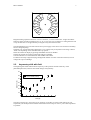
size reaches a minimum below slits=10. The vertical size remains the same.
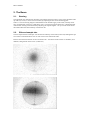
Pictures from the beam camera for slits=8 and slits=60 – the outline of the camera’s scintillator (6cm
diameter) and graticule can be seen. (Actual size)
DEVA Manual
5
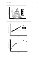
Profiles taken from the beam camera for a number of slit settings:
Horizontal profile (a.u.)
Slits:
4
8
16
24
32
40
60
edge of
scintillator
in camera
0
2
4
6
8
10
Width (cm)
The beam pictures can be fitted to a Gaussian profile. Parameters are shown here:
Spot Size (gaussian σ in cm)
2.0
1.5
width
height
1.0
0.5
0.0
0
10
20
30
40
50
60
Slits
5000
4500
Intensity at centre (a.u.)
4000
3500
3000
2500
2000
1500
1000
500
0
0
10
20
30
Slits
40
50
60
DEVA Manual
6
With a mask of 20mm diameter, a slit setting of 8 is found to give 75% of the muons on the sample. To
maximise the counts on a small flypast sample, use a slit setting of around 20.
The slits are adjusted from the rack in the kicker control area, down the steps behind EMU. Be careful
to adjust only the DEVA slits.
2.3.
Frequency response due to pulse width
At ISIS the muons are produced in large numbers in short pulses (about 80ns wide at half height) and
the approximation is usually made that an average arrival time near the centre of the muon pulse can be
used as time-zero. This is adequate if the time-scale of the evolution of the muon polarisation is long
compared to the width of the muon pulse but leads to difficulties in cases where the evolution is rapid.
The effect is seen clearly by considering a transverse field experiment performed at a succession of
magnetic fields. At low fields the frequency is small and the polarisation precesses with full
asymmetry. As the field increases there is an appreciable phase difference developed between muons
from the beginning and end of the pulse and the observed asymmetry falls. This frequency response has
been measured by observing the precession of muonium in quartz in small transverse fields, the results
are shown below.
Transverse Asymmetry
7
6
Quartz data
Theory
5
4
3
2
1
0
0
2
4
6
8
10
12
14
16
18
20
Frequency (MHz)
With RF precession measurements, where the muons are implanted in longitudinal field and then
rotated through 90º by an RF pulse, the pulse width does not matter. In this case the only limiting
factors on the frequency response are the precision of the detectors and electronics and the bin width of
the histogram.
2.4.
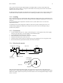
Detectors
The positrons produced when the muons decay are detected with scintillators linked to
photomultipliers.
DEVA Manual
7
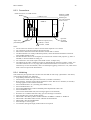
32
31
15
14
29
13
30
17
16
1
18
2
19
3
20
4
28 12
11
27
10
9
26
5
6
7
8
25
21
22
23
24
Diagram looking upstream. Detectors 1-16 are “forward”, 17-32 are “backward”. Angles around the
beam axis from vertically upwards are 24, 41, 58, 75, 92, 109, 126, 143 degrees. Looking from the side
or top the detectors are at approximately 45 degrees away from the beam axis.
The photomultipliers are powered from the Lecroy HV supply in the cabin. Users should not normally
have to change anything.
Channels 0-31 correspond to MCS histograms 1-32. Voltages may be anywhere in the range -1000 to
-2000 volts depending on the individual tube’s properties.
Select the channel to display by pressing CHANNEL and UP or DOWN.
Change the setpoint by pressing VOLTAGE and UP or DOWN.
Turn all channels on or off with the HV ON and HV OFF buttons.
If a detector develops a light leak (large background number of counts in the later time bins) turn its
voltage off to prevent damage.
2.5.
Asymmetry shift with field
The high magnetic fields affect both the trajectory of the positrons and the sensitivity of the
photomultiplier tubes, and can cause small changes of asymmetry.
23.0
normal mounting (α=0.79)
stick reversed (α=0.91)
22.8
asymmetry (%)
22.6
22.4
22.2
22.0
21.8
0
500
1000
1500
2000
Field (G)
The above graph is for a silver plate in two positions, in the flow cryostat. If this matters for your
experiment you should perform a similar measurement with a setup as close to your actual experiment
as possible.
DEVA Manual
2.6.
8
Time zero
This is the “average” arrival time of the muons in the pulse, measured from the start of the histogram. It
is calibrated by measuring muon precession in a series of different transverse fields and extrapolating
back to the point when all the phases are equal. The latest value is saved in the file “basetime.uda”
(kept in MUT$DISK:[MUTMGR.MUT_USERS.UDA] and copied to the current directory when
setting up the data analysis program UDA)
The value of t0 will be different between the Lecroy and DASH2 TDC systems and completely
different if triggering via a RF pulse generator. Cable lengths are significant: adding about 3m of extra
cable length moves the data by one 16ns bin.
The first good data bin is about 0.1 us after t0, when all the incoming muons have arrived. Some of the
detectors may also show a peak around time zero due to muons decaying in flight in the beamline and
the positrons produced not being properly focused and striking the detector directly.
For transverse field runs, the phase at time zero is actually about +3 degrees due to the rotation of the
muon spin in the kicker in a horizontal plane (actually the lack of matching rotation of the spin as the
muons are deflected by the electric fields). There is also a rotation of about 6.5 degrees in the vertical
direction due to the separator. The overall effect is that the muon spin points slightly up and to the left
(looking upstream), ie. towards detector 16. The combined spin rotation is visible as “wiggles” of
amplitude about 2.5% if looking at individual detectors in longitudinal field runs (20-200 Gauss).
26
Detector 1
Asymmetry (%)
24
22
20
18
16
14
0
2
4
6
Time (µs)
Silver, 100G LF (run 35709). Asymmetry plot of one detector only.
2.7.
Dead Times
If two muons decay within a short interval of time and their positrons both reach the same detector,
only one event may be counted. The minimum time to resolve two events is the “dead time” for that
detector. This effect causes distortion, mainly at the start of the histograms when the muon count rate is
highest.
Asymmetry plots tend to hide the distortion as both forward and backward counts are reduced.
The data can be corrected for this effect – our data analysis programs do this. However at very high
count rates the correction becomes inaccurate. A count rate of 20-30 Mevents/hour is a reasonable
compromise between high distortion and inefficient use of the beam.
The most recent calibrated dead time values are kept in the file DTMPAR.DAT in
MUT$DISK:[MUTMGR.MUT_USERS.RUMDA] . Another copy of this file is in the data directory
(MUT$DISK0:[DATA.MUT] or \\NDAVMS\MUTDATA as seen on the PC). If you are analysing
older data, old dead time files are preserved with names DTMPAR_date.DAT .
DEVA Manual
2.8.
9
Muon stopping range and sample thickness
The muons are produced with energy 4 MeV but slow down by interaction with matter. Their range is
dependent mainly on the mass per unit area. Some of this range is taken up by the beamline and
cryostat windows. Ideally all the muons should stop in your sample, not the window or the back of the
sample cell.
Range mg/cm
0
20
40
60
2
80
100
120
25
paramagnetic fraction
diamagnetic fraction
Asymmetry (%)
20
15
T20
some muons
in each
10
all muons reaching quartz
all muons
stopping
in Ti foil
5
0
0
2
4
6
Number of 30µm Ti foils
8
10
This measurement was taken in the “high temperature” flow cryostat. It uses a 2mm thick quartz
sample with a number of 30µm Ti foils in front, and a small applied transverse field. Signals from
paramagnetic muonium (in the quartz) and diamagnetic muons (some in quartz, full asymmetry in Ti)
are measured.
For a thin sample, a “degrader” of about 70mg/cm2 equivalent to 5 Ti foils can be used, including any
window on a sample cell. The sample itself should ideally have minimum “thickness” of 40 mg/cm2. It
is best to choose a degrader whose own muon signal is easily distinguished from that of your sample,
and add or remove foils to find the optimum thickness.
The degrader must be as close to the sample as possible, as it will scatter the muons and could increase
the muon spot size.
DEVA Manual
10
3. Sample Environment
3.1.
Flow Cryostats
There are two flow cryostats:
• The standard one with temperature range 3.5 to 400K, with an exit window
• The high temperature cryostat, with temperature range 4 to 600K.
Liquid helium is taken from a storage dewar via a needle valve and passes through the inner tube of a
concentric flexible transfer line. It flows through a heat exchanger near the sample before returning (as
gas) along the transfer line and to the pump. The sample is in a separate “static” exchange gas at
typically 10-15mbar. An ITC5 temperature controller controls the valve and heater.
The standard temperature flow cryostat, in its storage trolley (shown with the muon entry window
facing: when in the instrument it will be rotated through 180º)
MUSR2002 MUSR2002
Transfer tube port
Lifting eyebolts/bars
(removable if
required)
Sample stick access
Sample space
pumping valve
Heater/thermometer
connections
OVC pumping valve
Muon windows
The sample sticks are interchangeable but only those designed for high temperatures (with glass fibre
wrapping around the central rod) are suitable for use above 400K. Also ensure that your sample and its
coil or holder will cope with the expected temperature range.
3.1.1. Samples
The cryostat has helium exchange gas around the sample.
DEVA Manual
11
This cryostat can use the same sample holders as the EMU “Blue” cryostat: 37mm square with
mounting hole spacing 30mm, or a “flypast” holder made of a thin strip of silver sheet. The internal
diameter of the cryostat is 43mm.
For RF experiments the sample size depends on the coil used but a typical size is 25mm square and up
to 4mm thick. Powders must be enclosed in a non-conducting containter such as a Mylar envelope.
3.1.2. Installing
The cryostat fits into the top of the magnet frame, bolted to the support plate using 4 of the bolts on its
flange. Check the alignment with the laser and adjust the bolts holding the support plate to the frame if
necessary.
Use the appropriate ITC5 temperature controller for the cryostat (DEVA Flow 1 for the lower
temperature cryostat)
To minimise stress on the sample space windows ensure the cryostat vacuum space (OVC) is at
vacuum before pumping the sample space. Pump the OVC (lower of the two small taps) using a
portable turbo pump set.
3.1.3. Connections
•
•
•
•
•
•
Cryostat sample space port to a T piece. One branch goes to a rotary pump (with pressure gauge
and valve), the other has a valve and adaptor for the red helium line.
Cryostat heater/thermometer to ITC channel 1
Stick thermometer to ITC channel 2 (stick A) or 3 (stick B)
Transfer tube needle valve to ITC Aux. Out
Transfer tube gas outlet (at the top of the dewar leg) to the pumping box via a long plastic tube
Serial cable (from the optical fibre modem) to this ITC5 serial port
3.1.4. Mounting the sample
Length scale 19mm
Side view
70 mm
615 mm
Angular
scale 0 deg
Locking screws
Locating pin
on top flange
Muons
End view
Sample
With the standard blade and sample holder, the length from the bottom of the copper block to the
sample centre is 70mm and the top adjustment should be set to 19mm. If a non standard sample mount
differs from 70mm, adjust the top scale by the same amount. The overall length from flange to sample
centre is 615 mm.
DEVA Manual
12
For the standard blade, set the angle to 0 degrees. The muon arrival direction is in line with the locating
pin on the top flange and the sample plate should normally be perpendicular to this. You can rotate the
sample relative to the beam if required by your experiment, either now or when in the cryostat.
Steering curve in the Flow Cryostat on EMU
Slits 8, VSM=-0.1A, Fe2O3 with 20mm mask
18
16
Asymmetry (%)
14
12
10
8
6
4
2
5
10
15
20
25
30
Height of sample (mm)
3.1.5. Inserting the stick
The sample can be changed when the cryostat is cold, but heat it up to >25K first.
• Let the sample space up to 1 atm with helium.
• Remove the blanking plate
• Insert the stick: the pin on the stick flange should locate into the hole in the flange on the cryostat.
• If the cryostat is cold, the stick may not go all the way into the cryostat – the copper cylinder on
the stick is designed to fit tightly into the heat exchanger and thermal expansion can prevent it
fitting. Either leave the stick partially inserted and wait a minute, or warm the cryostat.
• Pump the sample space, purge two or three times with helium, and set the exchange gas pressure to
15 mbar.
3.1.6. Inserting the transfer line and cooling
This requires two people and you may also need a stool to be able to lift the transfer line high enough.
• Lift a Helium dewar onto the platform inside the area (requires someone with a crane licence).
• Remove the dewar neck insert/yellow valve by undoing the KF50 clamp and fit the one with the
level meter probe. Do this carefully but quickly to avoid getting air into the dewar.
• Connect the helium level meter cable.
• Remove the protective cover from the cryostat end of the transfer line. Check that the PTFE
sealing washer is present on the cryostat end of the transfer tube.
• Connect the needle valve cable. Turn the ITC5 on. This initialises the valve.
• Open the needle valve fully: press and hold “Gas Auto” and then press “Raise”. Check it stays in
Manual (light off).
• Insert the long leg of the transfer tube in the dewar. Be very careful not to bend the transfer
tube – the second person should support the cryostat end. Reduce pressure in the dewar as
required with the red valve. The tube should end up standing on the bottom of the dewar with
about 10cm length still visible.
• The second person should put the transfer tube into the cryostat once it will reach without
bending the dewar leg and tighten the locking nut. Turn on the diaphragm pump. Open the valve
on the pumping box. There should be a small but non zero flow.
• After about 5 minutes the flow should increase as liquid reaches the cryostat, and the temperature
will start to fall.
• The Green valve on the dewar should be open and the Red valve closed during operation.
DEVA Manual
13
If the cryostat is still not cooling after 20 minutes, the tube may be blocked with ice or solid air:
• Remove the transfer tube from the cryostat and dewar.
• Warm both ends with a hot air blower. Dry with paper tissues.
• Blow clean helium gas through it – use a piece of rubber tube over the cryostat end.
3.1.7. Computer control
Type @FLOW_ITC502 to set up the computer, then set temperatures with SET TEMP/SET=x. The
range is 4 to 400K for the low temperature cryostat or 4 to 600K for the cryofurnace. Temperatures
slightly below 4K can be obtained by careful adjustment of the needle valve in “manual” mode.
The computer uses two thermometers.
One is on the cryostat heat exchanger, labelled Readback on the computer and plotted as a dotted red
line on the graph. The temperature controller uses this to control the heater, and the computer uses it to
decide when the temperature is stable at a new setpoint.
The second is on the sample stick. This is labelled “Sample” on the computer, plotted as a solid white
line, and recorded in the log file.
3.1.8. Changing Samples
•
•
•
•
•
Warm the cryostat to 25K or above.
Remove the KF50 clamp holding the sample stick in place
Let the sample space up to 1 atm with helium
Remove the sample stick
Unless you have another sample stick ready, put the blanking plate on the cryostat and pump out
the sample space.
3.1.9. Changing the Dewar
Check the level regularly. Full is about 550mm, don’t go below about 50mm. A dewar may last from 2
days to a week depending on the temperature the cryostat is running at (below 10K uses rather more
helium). The sample can be left in place during the changeover although the temperature may rise.
• Turn off the diaphragm pump.
• Open the needle valve to 99.9%. Wait for the pressure on the pumping box to reach atmospheric.
• Remove the transfer line being careful not to bend its legs and put it in the support tray.
• Exchange the dewar, put the insert with the level meter into the new one.
• Warm the transfer line with the hot air blower and dry it with paper tissues.
• Blow helium gas through the transfer line for a minute or two – put the red gas line on the cryostat
end with a piece of rubber tube.
• Re-insert the transfer line as above. If the cryostat was cold, the temperature will rise initially until
liquid reaches it.
3.1.10.
•
•
•
•
•
•
•
Removing the cryostat
Warm the cryostat to 25K or above.
Ensure the needle valve on the transfer tube is open (set the ITC5 to Local, then press Gas Flow
and Raise) then shut the valve on the pumping box. The pressure should rise rapidly to 1 atm. If it
doesn’t, check with your local contact.
The transfer line can then be removed. Be careful not to bend either of the legs. Fit the protective
cover over the cryostat end of the transfer line and put the stopper into the cryostat.
Unplug all the electrical leads from the cryostat. Close the sample space valve and disconnect the
sample space pumping line.
Close the vacuum valve and switch off the turbo pump. Remove the vacuum line.
Unbolt the cryostat and lift it out.
Remove the level meter probe and replace the normal dewar neck insert.
DEVA Manual
14
4. Magnetic Fields
4.1.
Longitudinal Field
This is provided by the large water cooled Helmholtz coils, powered from a Danfysik supply located
next to the beamline magnet supplies. It is controlled from the computer in the cabin. The maximum
field is 2100 Gauss.
From MCS type “@LF0” to select it then “SET MAG/SET=x” as required.
4.2.
Transverse Calibration Field
This uses two small coils inside the main magnet, powered by the Thurlby Thandar supply in the cabin,
also under computer control. The maximum is 30 Gauss. The field is Vertical.
Type “@TF20” to turn it on and set 20 Gauss, and then “SET MAG/SET=x” if a different field is
required.
4.3.
Zero Field setting
This is automated using a triple axis fluxgate probe and three pairs of compensation coils. Control is
via a Labview program on the PC – under the “Zerofield” tab in Ray of Light, in turn controlled from
MCS.
Operating modes are:
• Auto Feedback: the probe is read and used to control the currents, to keep the field at the set point.
This is usually zero but can be any field up to the limit of the probe (5 Gauss) and in any direction.
This mode is activated by “@F0” in MCS.
• Manual: the probe is read but its value is not used. The currents are left at the last set values, or
you can type in new values. This is activated when one of the other magnets is selected in MCS.
• Dead Reckoning: the probe value is read but not used. The currents are adjusted as the main
magnets on the other instruments vary, to keep the field in DEVA steady. You can adjust the field
setpoint.
Either Hold Current or Dead Reckoning must be used if you are applying a field with the main
longitudinal or transverse coils, otherwise the zero field system will try to cancel it out.
DEVA Manual
5. Data Acquisition
5.1.
Electronics
Either the DASH2 system (as used on EMU or MUSR) or the Lecroy TDC can be used. The Lecroy
offers bin sizes down to 0.5ns for RF free induction decay runs (but it is best to select 2ns or above if
the high frequency response is not needed, as the bin sizes are non uniform at faster settings)
5.2.
MCS
MCS is the control program used to collect data. It is the same as used on EMU and MUSR.
For historical reasons the computer is called MUT, not DEVA, together with related things like the
account names and disks.
5.2.1. Running MCS
Log into the Alpha workstation (MUT) as user MUT. Ask your local contact for the password.
You should get a DECterm window. Type “MCS” to start the data acquisition program, which will
open some more windows.
15
DEVA Manual
16
5.2.2. Commands
NEW
STOP RUN
STOP RUN/AFTER=ee
START RUN
CLEAR
SAVE
SET TEMP/SET=t
SET TEMP/GAS=MAN
begin a run. Asks for details for the file header – does NOT
actually set the temperature etc.
pause data collection
arranges to pause the run when ee million positrons (MEvents)
have been counted (then you get a message and beep)
resume data collection
throw away data collected so far this run
save the run (and last chance to change the label)
SET TEMP/GAS=MAN=m
SET TEMP/GAS=AUTO
SET MAG/SET=m
set the temperature of the cryostat to t K
sets the helium valve to manual operation, leaving it at the
same setting
set the valve to position m (0 to 99.9%)
sets the valve to automatic when the next setpoint is sent
set the field to m Gauss
EXIT
RECOVER
@filename
SYS cmd line
end MCS
read in saved temporary data after a crash, then use SAVE
execute the script filename.COM containing MCS commands
execute DCL command cmd line
@F0
select zero field and enable auto zero feedback, all main
magnet supplies off
set up Longitudinal supply ready for use, set to zero
set 20G transverse field for calibration
set up for the low temperature flow cryostat
set up for the cryofurnace
@LF0
@TF20
@FLOW_ITC502
@HTFLOW_ITC502
@LECROY
@DASH2
SET MACQ/RGMODE
SET MACQ/NORGMODE
SET MACQ/RESOLUTION=p
SET HIST/LEN=l
SET HIST/GOOD=END=l /ALL
SET MACQ/READ=NFRAMES=n
set up the Lecroy TDCs
set up the DASH2 TDCs
set Red-Green mode
set normal acquisition
set TDC bin width in ps (usually 16000 or 8000 with the
DASH2 system, 500,1000,2000...16000 with the Lecroy)
to change histogram length in bins (both required)
SET MACQ/SAVE=s
read out data and change between red and green every n
frames (ISIS pulses) – typically use 500 to 5000
write data to disk every s readouts – typically 1 to 6
SET DISP/FIRST=f /NUM=n
SET DISP/LEFT=lll /RIGHT=rrr
which histograms to display
range of time bins to display
SHOW TEMP
SHOW TEMP/PAR
SHOW MAG
SHOW RUN
SHOW MACQ
SET LABEL
temperature values
temperature control (PIDs etc)
field value
counts per histogram, etc.
data acquisition parameters
change the label (header) of the current run (if unsaved) or that
to be used for the next run
5.3.
Scripts
The program MKSCRIPT2 is used to write scripts.
From MCS type SYS RUN MKSCRIPT2 , or from another DECterm window type RUN MKSCRIPT2
DEVA Manual
17
Select from the menu using the initial letter of each command or the arrow keys, then RETURN. The
mouse will not work.
Add: add an entry to the script. This can scan through several fields or temperatures taking a run at
each. Press RETURN to use the default KEEP if a value is the same as the previous entry rather than
retyping the same temperature or field – this also makes the script run faster as it doesn’t have to wait
for stabilisation each time.
T20: add a T20 measurement run (selects Transverse field and sets it to 20 Gauss, collects data, then
selects the Longitudinal supply again)
Delete: remove an entry
Undo: reverse the last change
Read: read in a previously saved script for editing
Write: write the script to disk so that MCS can run it
Print: print a summary of the script (if you do this after Write, it puts the script name on the printout)
Help: simple online instructions
Quit: return to MCS or the DCL command line
Use the PAGE UP/PREV and PAGE DOWN/NEXT keys to scroll through the script if it is too long to
fit the screen.
Putting KEEP for both the field and temperature of the first entry means it assumes you will have
already set the temperature/field and started the run and the script only waits for the required counts.
Putting a count limit of 0 for the last run means it leaves the run counting when the script finishes, and
you have to stop and save it manually.
To scan temperature or field, type first last step at the Temperature or Field prompt, instead of a single
number. The last value wil be rounded if required to give a whole number of steps of the size specified.
The number of steps calculated is printed as confirmation. You can scan up or down, enter a positive
value of step in both cases. You cannot scan temperature and field at the same time.
You can also scan fields on a log scale (up or down). Enter first last –runs where runs is the number of
runs required. The ratio between successive fields will be printed as confirmation.
Normally fields in a script mean Longitudinal, and you should be sure the longitudinal field is selected
with @LF0 before starting a script which is to set fields. If you execute a script when the Transverse
supply is already in use, any field setpoints will use it (until a T20 entry is reached).
The script will update the field and temperature values in the label (file header) when it changes the
actual field or temperature. Before running a script that starts the first run itself, check that the other
entries (sample name, comments, etc) are correct. Set them with the MCS command SET LABEL.
The script is saved in a file of the form name.COM
To run it: type “@name” in MCS.
To interrupt a script in progress: press CTRL-C.
This does not stop the current run, although the run will stop when the pre-set number of counts are
reached. You can stop and save the run manually.
To resume the script, first read it into MKSCRIPT2 and edit it to remove the entries which have been
run. Also you may need to change the current run (which will now be the first in the script) to have
KEEP for temperature and field. Write it back to the file, exit MKSCRIPT2 and restart with @name.
Experienced users may want to edit their scripts with the VMS editor. They contain a header which
MKSCRIPT uses when reading a script in, but is ignored by MCS (each line starts with “!”.) This is
followed by the actual commands executed by MCS.
DEVA Manual
18
6. Computing and Data Analysis
6.1.
•
•
•
•
•
Computers
MUT (Alpha/VMS workstation): the instrument data acquisition computer. Can also be used to
access ISISA.
ISISA (Alpha/VMS central server): available for data analysis with UDA, etc.
User PC (Windows): available for data analysis. Has WiMDA, Origin, Microsoft Office, Internet
Explorer, etc. and eXceed to connect to the VMS machines.
Labview PC (Windows): controls the zero field and other sample environment. Not for general
use.
A Unix / Linux service is available, contact Computer Support. Access is via Telnet or eXceed
from the PC.
6.2.
MUT01 and UDA
The account MUT01 is available for VMS data analysis. Alternatively you can use your own account.
Log in to the account MUT01 using Exceed on the PC, using SET HOST ISISA in a spare DECterm
window on MUT, or Telnet to isisa.nd.rl.ac.uk from off site. Ask your local contact for the password.
Select one of the user areas offered by typing the name (or ask your local contact to set up a new one).
Next type SETUP
Now you can use UDA etc as on EMU or MUSR. For instructions on using UDA, see the next chapter.
The nearest printer is SYS$LSR10 just outside the EMU cabin. Others are SYS$LSR5 in MUSR or
SYS$LSR2 in the DAC.
6.2.1. Convert_ASCII
This converts the binary data files produced by MCS into ASCII suitable for reading into general
purpose data analysis programs or spreadsheets. Type CONVERT_ASCII.
The output formats are:
• Histograms listed individually (.USR format)
• Histograms as columns, with a time column at the left (easier to read in)
• Asymmetry and its error bars
There is an option to apply dead time correction to the data. Depending on the format, you can also
specify alpha, the detector grouping and time zero.
A batch of files can be converted at once.
6.2.2. TLOGGER
Type TLOGGER to run the program to plot out the temperature log files. Printouts are left in files
named PGPLOT.PS in the current directory, with one file version per run plotted.
Print them with PRINT /QUEUE=SYS$LSR10 PGPLOT.PS;*
6.2.3. RUMDA
This is available on VMS. See the separate manual.
6.3.
WiMDA
This is set up on the PC in the cabin. See the separate WiMDA Manual for instructions. You should
make your own subdirectory under D:\users and store temporary files there. The PC disks are NOT
backed up, and old files may be deleted to free up disk space, so take a copy of anything valuable when
you leave.
The data is accessed via the shared drive \\NDAVMS\MUTDATA . From other PCs on site you may
need to connect to it before WiMDA can load data.
DEVA Manual
6.4.
19
Taking your data home
6.4.1. FTP
From outside ISIS connect to isisa.nd.rl.ac.uk and log in either under your own account or MUT01.
Alternatively use the FTP command on VMS or WS-FTP on the PC to PUT files to your own FTP
server.
Data recently collected is in MUT$DISK0:[DATA.MUT]Rnnnnn.RAL and temperature logs in
MUT$DISK0:[DATA.MUT.TLOG]Rnnnnn.TLOG
Data restored from the archive is in SCRATCH$DISK:[MUTMGR.RESTORE]
Files created by UDA, CONVERT_ASCII, etc are in SCRATCH$DISK:[MUT01.USERS.areaname]
Raw data files must be transferred as Binary, TLOGs as ASCII.
There is no FTP access into the PC network or off site access to shared PC drives.
6.4.2. CD-ROM
The PC in the cabin has a CD writer. Files should be copied to the local disk first. Ask your local
contact for a blank disk. If you are taking raw data files, you should also take a copy of the dead time
calibration file.
6.5.
Archiving
All data is written to the ISIS data archive as soon as it is saved from MCS. The original files are kept
on the local disk as long as space permits – usually a year or so.
To restore data for runs run1 to run2 inclusive type (in VMS)
RESTISIS mut run1 run2
and for temperature logs
RESTISIS –l mut run1 run2
Data is put into SCRATCH$DISK:[MUTMGR.RESTORE] where our standard programs know to look
for it.
Use RSTATUS to show the progress. Some files are on tape and must be manually loaded during the
next working day. More recent files may take only a few minutes to return.
DEVA Manual
20
7. UDA
7.1.
Introduction
UDA is the simplified µSR data analysis program. There are three menus in UDA, the Main Data
menu, the UDA data Grouping menu and the UDA data Analysis menu.
On start-up the program will always enter the Main menu. At this menu you can read and write data
files, plot spectra and make changes to the data loaded.
In the data Grouping menu you can select how to map your raw histograms into the "groups" that are
used when plotting or analysing. Two different grouping schemes can be used, the Simple (straight,
TF) grouping, or the F-B (LF,ZF) grouping. Deadtime correction of data is available using the same
correction method as the RUMDA analysis program.
In the Analysis menu you can select a model function and make a least-squares fitting of the model
parameters. The fitting result can also be plotted from this menu.
7.2.
Running UDA
To access UDA from account MUSR01 type SETUP followed by UDA as described in section 6.3.
This will run the most recent version of UDA. The display will be redrawn as a dashboard and the
cursor will automatically select the option MCSFILE in the Main menu. To select any other item from
the menu use the cursor (arrow) keys or simply type the first letter of that item (e.g. ‘P’ for PLOT).
7.3.
The Main Data Menu
The Main Data menu allows you to read, write and modify experimental data. The options available
from this menu are listed below. Plotting of error bars on data points can be turned off/on using the
SETUP option.
MCSFILE
USRFILE
OLDFILE
WRITE
INSPECT
GROUP
CHANGE
PLOT
ANALYSE
SETUP
HELP
QUIT
7.4.
Read a MCS run file in the format used by the data acquisition software
Read a uSR file from the disk
Read one of the old (PDP) run files
Write (grouped) data to a uSR file
Inspect run and all histograms
Enter the Grouping Menu
Change run file parameters
Plot one or more groups on the terminal screen
Enter the analysis menu
Set program configuration parameters
Enter the VAX/VMS help facility to read the UDA help library.
Exit UDA and return to VMS prompt
The Grouping Menu
The grouping menu is accessed through the option "Group" from the Main menu, and defines the
grouping and correction of raw histogram data. There are currently two ways of grouping the
histograms:
a) the Simple grouping, where histograms are simply added together.
b) the Forward-Backward (F-B) grouping, where the 'asymmetry ratio'
(F-αB)/(F+αB) is calculated.
Deadtime correction of data is turned on/off using the DeadT option. To compensate for deadtime,
UDA uses the same file of deadtime values as the RUMDA analysis program, generated at the start of
each cycle from a long silver run. Please ask your local contact if you are analysing data from a
DEVA Manual
21
previous cycle and so require UDA to use deadtime values from that cycle rather than the current
deadtime file. The effects of deadtime correction are shown in section 2.7.
The options available for grouping and correcting data are shown below.
CHANGE
READ
WRITE
DEADT
ALPHA
GUESS
BUNCH
HELP
EXIT
7.5.
Change histogram grouping
Read grouping table from disk
Write grouping table to disk
Switch deadtime correction on/off
Select (F-B) scaling factor
Estimate alpha for a T20 run
Setting the bunching to ‘n’ adds ‘n’ bins together.
Display help text. (Don't panic)
Return to UDA Data (main) menu
The Analysis Menu
The Analysis menu is entered by selecting the option ”Analyse” in the UDA Main menu. Using the
options outlined below it is possible to select a model function and make a least squares fit of the
model parameters. The results of the fit can also be plotted and output to an ASCII file.
SELECT
PLOT
FIT
HELP
VALUES
THEORY
ALPHA
UNDO
EXIT
WRITE
READ
DIST
7.6.
Select a group and a bin range to work on.
Plot the data and the fit; allows fit to be written to an ASCII file
Run fitting routine using the starting values displayed in right hand window
Enter the help system at the Analysis menu level
Enter the parameter display to change parameter values/status. To move in the parameter
display use UP or DOWN cursor keys. To change a value use the ENTER key. Status
codes are changed by typing ~ (vary parameter), ! (fix parameter), = (tie parameters
together). Return to the menu by the left or right cursor keys.
Select a theory function, number of sub-components and lineshape
Change value of alpha
Undo fit and restore original parameters
Exit this menu and return to the main UDA menu
Write parameters out to a file
Read parameters in from a file
Distribute parameters to all groups (necessary for transverse geometry)
Computer files
These files must be copied into the area you are working in. If the area has been selected by SETUP (as
described in section 6.2) they will have been copied to the new area automatically.
SETUP.UDA
BASETIME.UDA
TRANS.UDA
LONG.UDA
PDF.UDA
UDAHELP.HLP
7.7.
UDA reads some variables from the file SETUP.UDA. In particular the
directory address of the data is set up in this way. Of particular interest are the
FORTRAN format strings used to convert a run number to a full file name.
contains the value which UDA will use for time-zero (see section 2.6).
default transversal grouping
default longitudinal grouping
parameter definition file
help library source, UDA matters
Theory functions defined in UDA
A number of theory functions are predefined in UDA:
DEVA Manual
22
7.7.1. Longitudinal and zero field
Function Name
1. Lorentzian
2. Gaussian
3. LX(exp) - Stretched Exponential
4. Keren LF (extended Abragam)
5. Kubo-Toyabe (Gaussian)
6. Kubo-Toyabe (Lorentzian)
8. Dynamic Kubo-Toyabe
Note 1:
Definition
a o exp( − λt )
a o exp( − (λt ) 2 )
a o exp( − ( λt ) β )
a 0 exp ( − Γ(t)t) ; see note 1 below
a o ( 1 3 + 2 3 (1 − ( λt ) 2 ) exp( − ( λt ) 2 2))
a o ( 1 3 + 2 3 (1 − λt ) exp( − λt ))
see note 2 below
2∆2
Γ (t)t = 2 2 2 {[ωs2 + ν 2 ]νt + [ωs2 − ν 2 ] ×[1 − exp(−νt)cos(ωst)] − 2νωs exp(−νt)sin(ωs t)}
(ωs + ν )
where UDA’s sigma is equivalent to ∆, UDA’s tau is equivalent to 1/ν and ωs=γµB0.
Note 2: Function 8, the dynamic Kubo-Toyabe, uses numerical integration to produce the fitting
function and so requires more time than the other functions. Only fit up to channel 1000 when using
this option.
7.7.2. Transverse field
Function Name
11. Lorentzian with freq
12. Gaussian with freq
13. LX(exp) - Stretched Exponential with
freq
14. Abragam with freq
7.8.
Definition
a o cos(ωt + φ ) exp( − λt )
a o cos(ωt + φ ) exp( − ( λt ) 2 )
a o cos(ωt + φ ) exp( − ( λt ) β )
a o cos(ωt + φ ) exp( − (λτ c ) 2 (exp( − t τ c ) − 1 + t τ c ))
Time-zero
UDA reads the file basetime.uda to get the value of time zero used in the fits. See section 2.6 for the
definition.
DEVA Manual
23
8. RF and other special setups
There are cables between the area and the cabin labelled X1,X2,X3.
In the cabin these cables come to the patch panel at the bottom of the rack, together with the Cerenkov
signal (cable C3) and the Extract Trigger (cable EX3).
8.1.
Timing and Acquisition
Normal setup: the Cerenkov goes via a discriminator to the Frame Start on the TDCs. Red/Green from
the TDC can be connected via one of the cables to the RF rack. Usually the Extract trigger will be used
to time the RF pulse.
Special setups: the Cerenkov or ISIS Extract Trigger signals can be used to trigger the RF, which in
turn triggers the data acquisition.
8.2.
The Lecroy TDCs
8.2.1. Specifications:
Bin width selectable 0.5 to 16ns in powers of 2 (non uniform below 2ns: care!)
32 histograms of up to 8192 bins each, for each of Red and Green
Maximum time length of histogram 32µs
Either frame-by-frame or block-at-a-time red-green mode can be used. In frame by frame mode you
can select from n=1 to n=126 green frames for every red frame, giving red frame rates between 25 Hz
and 0.4 Hz.
Note that the header of the saved file indicates the number of frames in the red histograms, but for n>1
the green histograms contain more frames worth of data. Take care when analysing this data, especially
when applying dead time corrections.
8.2.2. CAMAC Modules:
LP: Hytec 1341 List Processor with 256k word data store
Dis: Lecroy 3412E discriminator
TDC: Lecroy 3377 time to digital converter
PCR: Nuclear Enterprises (Harwell) Preset Counting Register
ECC: Hytec 1365 Ethernet Crate Controller with 4M RAM
DEVA Manual
24
8.2.3. Connections
Frame start (ECL) to COM on TDC
CAMAC crate
LP Dis tdc Dis pcr
1-8
1724
free slots for
GPIB etc
ECC
Ethernet to FEM
second (private)
ethernet port.
Via hub if another
crate is in use
addr 20
A
916
Inputs from
photomultipliers
2532
Red/Green outputs (TTL)
A: 0=Red, 1=Green
*UHHQ 5HG
Optional
terminal
9600 baud
Notes:
• The List Processor must be in station 1 and the others adjacent to it as shown.
• No connections to the front panel of the List Processor
• Short ribbon cables between the discriminators and the TDC as shown.
• The Discriminators are usually in Manual operation, set the thresholds and widths on the front
panel. Widths should be 10ns.
• The discriminators have 2 sets of outputs, the second can be used for other purposes, eg. fed to a
DASH2, to check thresholds or timing, etc.
• No connection to the counter inputs of the PCR. Use the A outputs only.
• The TDC does NOT like a double start pulse as obtained directly from the Cerenkov counter. Use
a first discriminator set to a very large pulse width which then drives a second one set to 10ns.
Alternatively use one discriminator, with a second output triggering a timer set to 1µs, which is fed
back to the Veto input of the discriminator.
8.2.4. Initialising
This should only be required if the crate has been switched off. The script “@LECROY” will do this,
with some help from the user, otherwise:
• Stop MACQ if MCS is already running
• Disconnect the Frame Start pulse from the TDC (or disable it elsewhere)
• Reset the ECC: push the switch to Reset and back to Norm. Wait for it to initialise (10 seconds):
message appears on the terminal if attached.
• $ ECCOP/SETLAM=3 20 (assuming crate address is 20)
• $ ECCOP/SETLAM=5 20
• $ ECCOP/COMMAND_LOAD=some$disk:[some.dir]LTDCFF.S /ID=4 20
• $ ECCOP/BOOK=1 20
(this runs the downloaded code, more messages appear on the terminal)
• Reconnect or re-enable Frame Start. May give more messages on terminal.
• Now start MCS if it was not already running
• MCSCONF> SET MACQ /DEV=LTDC /CRATE=20 /FIRST=1 /NDEV=1 /NHIS=32
• MCSCONF> SET FREG /DEV=LTDC /CRATE=20 /STATION=1
• MCSCONF> SET SGATE/DELETE
• Start MACQ if it was stopped
• set resolution, histogram length, readout interval as required.
DEVA Manual
25
8.2.5. Setting up
To select the data acquisition mode:
• To enable Frame by Frame – n Green frames for every 1 Red
MCS> SET MACQ/RGMODE=n
(eg. SET MACQ/RGMODE=1 gives 25 Hz, SET MACQ/RGMODE=4 gives 10 Hz, etc)
• To collect data in blocks of red and green:
MCS> SET MACQ/RGMODE=0
• To turn off red/green completely – single set of histograms
MCS> SET MACQ/NORGMODE
Now collect data as usual!
8.2.6. Timing notes
In Frame by frame mode the Red/Green output changes after each frame, whether or not MCS wants
the data. Therefore the lamp / RF pulse / etc runs at a steady frequency and any sample heating should
be constant.
The output usually changes at about 175 µs after the Frame Start, but can be later if the crate controller
was busy receiving data from the Ethernet when the TDCs finished collecting data. Do not use it as a
time reference, only as a veto or enable signal.
When driving “slow” equipment such as the flash lamp from the previous frame’s Extract Trigger, the
usual method is to use a delay set to about 19ms which then drives an adjustable delay of about 1ms.
For correct operation, connect the Red/Green signal to the Veto of the last delay stage or the lamp
itself. Vetoing the first 19 ms delay unit would get Red and Green the wrong way round (as compared
to block red-green where this does not matter).
Once set up, Frame by frame mode actually turns on (or off) on starting the next run, when you type
<return> or Y <return> to the “Clear Devices?” prompt.
8.2.7. Discriminators
These are normally set up manually from the front panel, with threshold levels of 50 or 75 mV and
pulse width 10ns. Users should not need to change anything. However it is possible to use a program
on the FEM to put these in Remote mode and then program the threshold levels.
Neither MACQ nor the downloaded program LTDCFF accesses them directly.
DEVA Manual
26
9. Troubleshooting
If you have to reset any equipment as described below, remember to tell your local contact as soon as
possible – it may indicate that something is about to fail completely or needs repairing.
9.1.
No muons (or far fewer than expected)
First check:
• The Frame Start light on the DTU module in the DASH2 TDC rack is lit - if not, the beam is off
or there is no start pulse from the Cerenkov detector. Frame Start flashing means ISIS is at base
rate (1/32 of 50Hz).
• If Frame Start is present, is the computer reading back from the electronics? Type SHOW RUN
• Is there any beam going to the other muon instruments?
9.1.1. Beam Off
Check the proton beam current – the big display in the hall or the ISIS PPP Monitor program on the
PC. The last hour graph on the ISIS web page only updates every 10 minutes.
9.1.2. Kicker
The racks in the kicker control area (down the steps behind EMU) are:
Momentum slit (do not
touch)
Beam slits for each
instrument
HV for Cerenkov (start
pulse) detectors
Kicker HV supply
Kicker monitor scope
Kicker main control
panel
Thyratron
Separator HV supply
Old UPPSET unit
(not in use)
If the kicker trips off, DEVA and EMU have no beam and MUSR will have a double pulse with twice
the usual rate. Some lights will be lit on the control panel but the HV supply will be off. Instructions
for resetting it are attached. Check with the other users before doing anything.
The kicker status is indicated in the MCR – someone from the crew may reset it.
9.1.3. Beamline Magnets
When one of these trips the beam may be lost completely or just reduce in rate and have a huge spot
size.
Magnets Q1-Q9, B1/2 and the Separator are common to all three beamlines. B1/2 goes off if any of the
Muon Beam Off buttons are pressed, and the white lights will come on in all the areas. Warning: it is
possible to press a button gently (accidentally) without it latching in yet trip the beam.
Septum A and Q10A-Q12A are for the DEVA branch only. B is MUSR, C is EMU.
The Switchyard magnets are normally off .
The magnet supplies are located on the platform at the far end of the hall. Each position is labelled with
the required current for that magnet.
Reset1 Separat
Q2
Q1
on/off
Q3/5
spares spares
Q4
Q6
on/off
Q7
Q8
Q9
on/off
B1/2
spare
DEVA DEVA EMU Reset2 Q10A
Helm- Septum Septum
Q11A
holtz
A
C
PLC
on/off
Q12A
spare
Q11B
on/off
Q10B
SWY1
Reset1: interlocks with reset buttons for Q1-Q9, B1/2 and the Separator supplies
Reset2: interlock reset buttons for Q10A-Q12C, Septum, Switchyard and instrument magnets.
Q10C
Q11C
on/off
Q12C
SWY2
DEVA Manual
27
on/off: panel with ON and OFF buttons for the power supplies.
spare: Spare supplies, not connected or powered up. (ISIS staff use only!)
The PLC has status lights for the second group of magnets and for the shutters: the upper row of
modules show inputs from various sensors and switches and the lower row is the outputs to enable the
supplies. For interlocks the general rule is Lights ON = good, lights OFF = tripped.
Farnell supplies: press the interlock reset buttons then the green ON button next to the power supply. It
should not be necessary to touch the controls on the supply itself. Check it returns to the setpoint and
the green “Output Enable” light is on.
Danfysik supplies (septum): press the interlock reset buttons, then on the supply itself press OFF/Reset
and then ON. Check the setpoint and readback values.
The Separator electric field is provided by the Glassman unit in the rack next to the kicker. The usual
value is 90kV.
9.1.4. Photomultipliers
These are powered from the Lecroy HV supply in the cabin.
Turn all channels on or off with the HV ON and HV OFF buttons.
The Cerenkov start counter is supplied from the HV supply next to the slit controls – check the other
instruments are counting data OK.
9.1.5. Beamline Vacuum
This is monitored on the rack on the platform, above the target/kicker control area. Check that the
vacuum in the beamlines is OK (about 10-6 mbar or better) and that all the valves are open except for
those labelled “vent” and “bypass”. The “line” valve in each branch of the beamline is linked to that
instrument’s shutter. Do not attempt to open or close valves – ask your local contact or the MCR for
advice.
9.1.6. RF triggering
Is the data acquisition being triggered from the RF zero crossing – if so is it working properly?
9.1.7. Computer
There may be muons but the computer is not reading back from the electronics. See below.
9.1.8. Blocker Closed ?
The blue lights in the area will light if the blocker has been opened correctly.
9.2.
Strange data
9.2.1. Light leaks
On an asymmetry vs. time plot this gives asymmetry going to +100% or –100% at later times.
If a detector develops a light leak (large background number of counts in the later time bins) turn its
voltage off to prevent damage.
9.2.2. Beamline Magnets
If a beamline magnet trips there may still be muons but the spot size could be huge and the asymmetry
change to an implausible value. Reset it as above.
DEVA Manual
28
9.2.3. RF pickup
With high RF pulse power, it can be picked up by the detector wiring. This may change the sensitivity
of th electronics when counting actual events or even make it count cycles of the RF waveform. First
try to improve the shielding of the coil or insulate it from the spectrometer’s metal framework.
Changing frequency (if possible) often helps as the pickup is via resonances in the cables etc.
If the problem is not too severe, just remove that histogram from the grouping when analysing the data.
If it has a huge count rate it may be necessary to disconnect that detector from the electronics in the
cabin, so that the total counts in the run correspond to usable events.
9.3.
Computer
The PF1 key locks/unlocks the screen (or the currently selected Decterm window). This can give the
appearance of a crash, and can actually cause a crash if left locked for too long.
Many problems with MCS can be cleared by restarting it:
• first SAVE the current run. If it refuses to do this, you have to kill MCS itself from another
Decterm window.
• type EXIT
• Wait a few seconds for all the windows to disappear
• If any remain, type SHOW SYSTEM to get the list of processes. Look for MTEMP, MMAG,
MACQ, MWSDISPLAY and MWSWINDOWS. Kill them with STOP /ID=nnnnnnnn where
nnnnnnnn is the number to the left of the process name.
• type MCS to restart.
No communication with the data acquisition hardware: from MCS type SYS SHOW SYSTEM and
look for the process name ecc_1365. If missing, it usually requires a reboot to get it going again.
Warning: closing the DECterm window in which MCS is running using the “close” icon usually kills
the ecc_1365 process!
No communication with Labview: from MCS type SYS SHOW SYSTEM and look for the process
name DCOM$RPCSS. If missing, it usually requires a reboot to get it going again. If you find
DCOM$STARTUP-** instead, this indicates it has failed to initialise correctly: in this case contact
Computer Support.
If all else fails, there is a reset button on the Alpha workstation. Log out first if possible, then press this
to reboot.
9.4.
Magnets
9.4.1. Main field
If the Danfysik Longitudinal field supply trips, MCS will print error messages every few seconds. One
or more red LEDs will light on the supply control panel. Pressing the buttons next to them will indicate
exactly what it thinks is the problem. MAG Overtemperature can mean the “Helmholtz Interlock” key
by the door.
• In MCS type @F0 to stop the error messages.
• Clear the problem: if it was the door interlock, close the door and raise the blocker. If a problem
with water flow, press the three reset buttons on the interlock PLC rack.
• Reset the power supply: press LOCAL to make the Remote light go out, then OFF/RESET which
should turn off any red lights, then Remote.
• In MCS type @LF0
• Then type SET MAG/SET=xxx to go back to your setpoint.
9.4.2. Zero field
The Zero field program on the PC will give a status message of “Current Overload” if it is unable to
reach zero (or its setpoint). This may be due to:
DEVA Manual
•
•
•
29
Set point too large: the maximum available from the coils is about ±1 Gauss (1000 mG as shown
on the PC) in each Transverse direction and ±3G in Longitudinal. The magnetometer range is ±5G.
The main LF or T20 magnet is on: this should not happen if controlled from MCS.
There is a fault with the coils or magnetometer.
9.5.
Temperature control
9.5.1. Needle Valve
Sometimes the ITC temperature controllers can lose the zero position on the motorised valve, leading
to excessive helium use and high heater power with the valve reading 0%, or the temperature drifting
up with the valve apparently at 99%. The latter could also be due to an empty dewar. To reset:
• Switch the ITC off and on again
• Wait for it to initialise the valve (light flashing)
• Re-send the setpoint with SET TEMP/SET=ttt
9.5.2. Empty Dewar
Don’t let the dewar run dry if possible! If this happens:
Turn off the diaphragm pump immediately.
Check the pressure gauges on the dewar and the pump control box. If below atmospheric you have to
admit clean helium from the supply on the panel via the red valve on the dewar. Gas will come out of
the green non return valve once you are back at atmospheric pressure. It may take several minutes.
Now remove the transfer line as usual and change to a new dewar.
DEVA Manual
10.
30
Contacts and further information
Address:
ISIS Facility
Rutherford Appleton Laboratory
Chilton
Didcot
Oxon OX11 0QX
U.K.
Phone (Main switchboard) 01235 821900
Fax (User Office) 01235 445103
Fax (ISIS Staff) 01235 445720
Web page http://www.isis.rl.ac.uk/muons/
Ordinary phone extensions (starting with 5 or 6) can usually be dialled from outside the lab with 01235
44+ext or +44 1235 44+ext from abroad. Mobile short codes starting with 1 only work on the RAL
exchange.
To make outgoing calls just dial the full number. There is no need to add a leading “9”.
10.1. Muon Group
Dr. Steve Cottrell
Prof. Steve Cox
Dr. Gordon Eaton
Dr. Adrian Hillier
Dr. Clive Johnson
Dr. Philip King
Dr. James Lord
Dr. Francis Pratt
Office phone
5352
5477
5464
6001
6259
6117
5674
5135
Mobile short code
1665
1476
1716
1101
1114
E-mail
[email protected]
[email protected]
[email protected]
[email protected]
[email protected]
[email protected]
[email protected]
[email protected]
10.2. Useful Phone numbers (RAL)
ISIS Main Control Room (MCR)
Emergencies: Fire/Ambulance
Occupational Health (minor illness)
Security lodge (main gate)
Health Physics (sample checking)
DEVA Cabin
MUSR Cabin
EMU Cabin
ARGUS (RIKEN) Cabin
User Office
Local taxi bookings to B&B or station
Airport transport
Technical support
Computer support
6789
2222
6666
5545
6696
6851
6135
6831
6766
5592
User Office 5592 in working hours, MCR 6789 out of hours
User Office 5592 – give 24 hours notice.
see the list in the cabin. Out of working hours phone the
MCR who will contact someone on call.
1763 (working hours)
DEVA Manual
31
10.3. Transport
Trains
National Rail
Enquiries
Buses
Oxford Bus
Company
Stagecoach
08457 484950
http://www.railtrack.co.uk/
It is usually possible to arrange a
taxi to either Didcot or Oxford
station.
01865 785410
http://www.oxfordbus.co.uk/
01865 772250
http://www.stagecoachoxford.co.uk
Local buses and coaches to London
and the airports
Local buses – some serve the
Harwell Business Centre bus park
opposite the RAL main gate
Air
BAA
http://www.baa.co.uk/
Flight arrival/departure information
for Heathrow and Gatwick airports
10.4. General Information
Oxford Tourist Information Centre
Oxford Guide on the Web
01865 726871
http://www.comlab.ox.ac.uk/archive/ox/
10.5. Eating and Drinking
Didcot Tandoori, 222 Broadway, Didcot
Cherry Tree Inn, Steventon
The Crown and Horns, East Ilsley
Fleur de Lys, East Hagbourne
The George and Dragon, Sutton Courtenay
The Great Western Junction Hotel, Didcot
The Hare Inn, West Hendred
The Harrow, West Ilsley
The Plough, Sutton Courtenay
Red Lion, Drayton
Rose and Crown, Chilton
The Swan Inn, Sutton Courtenay
The Wheatsheaf Inn, East Hendred
01235 812206
01235 831222
01635 281205
01235 813247
01235 848252
01235 511091
01235 833249
01635 281260
01235 848801
01235 531381
01235 834249
01235 847446
01235 833229