Download The MuSR User Guide

The MuSR User Guide
AD Hillier, PJC King, SP Cottrell,
and JS Lord.
ISIS Facility, CCLRC Rutherford Appleton Laboratory
February, 05
1. Introduction
Contents
CONTENTS
1. INTRODUCTION
1.1 Setting up an experiment
1.2 The MuSR area interlocks
1.2.1 Closing the area
1.2.2 Entering the area
2. THE MUSR SPECTROMETER
3. SAMPLE ENVIRONMENT
3.1 Dilution refrigerator
3.2 Sorption cryostat
3.3 The Oxford Instruments Variox cryostat
3.3.1 Removing a sample
3.3.2 Loading a sample
3.3.3 Operation above 4.2 K
3.3.4 Operation below 4.2 K
3.3.5 Filling with Helium
3.3.6 The Oxford ITC503 Temperature Controller
3.4 Orange cryostat
3.4.1 Removing a sample
3.4.2 Loading a sample
3.4.3 Cooling the cryostat to 4.2 K
3.4.4 Cooling the cryostat below 4.2K
3.4.5 Filling with Helium
3.4.6 Care of the cryostat when not in use
3.4.7 Additional notes
3.5 Flow Cryostat
3.5.1 Sample holder
22/02/2005
1 - Introduction
3.5.2 Installation
3.5.3 Connections
3.5.4 Inserting the stick
3.5.5 Cooling
3.5.6 Removing
3.6 Closed-cycle refrigerator (CCR)
3.7 Furnace
3.7.1 Sample mounting
3.7.2 Mounting the furnace on the instrument
3.7.3 Connections
3.7.4 Eurotherm set-up
3.7.5 Controlling the furnace
3.7.6 Typical data collection parameters
3.8 Temperature control files
3.9 Sample mounts
4. MAGNETIC FIELDS
4.1 Zero field compensation
4.2 Calibration field
4.3 Applied fields
4.3.1 Effects of the finite muon pulse width on useable transverse fields
4.3.2 Effects of high longitudinal fields on asymmetry
5. BEAM SIZE, EVENT RATE AND STEERING
5.1 The muon beam spot size
5.2 The event rate
5.3 Steering the beam
6. COMPUTING
6.1 General Information
22/02/2005
1. Introduction
6.2 Data acquisition
6.3 Data analysis
6.3.1 Logging on
6.3.2.
Using the MUSR01 account for data analysis
6.3.3 Using your own account for data analysis
6.4 Utility programs
6.4.1 CONVERT_ASCII: converting data files to ASCII format
6.4.2 TLOGGER: plotting TLOG files
6.4.3 ISISNEWS: the status of ISIS
6.4.4 Archiving data on to a PC floppy disk
6.5 The MuSR PC
6.6. Printers
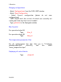
7. DATA ACQUISITION: SECI
8. DATA ANALYSIS: UDA
8.1 Introduction
8.2 Running UDA
8.3 The Main Data Menu
8.4 The Grouping Menu
8.5. The Analysis Menu
8.6 Computer files
8.7 Theory functions defined in UDA
8.7.1 Longitudinal and zero field
8.7.2 Transverse field
8.8 Time-zero
9. OTHER COMPONENTS OF THE MUON BEAMLINES
9.1 Beamline power supplies
22/02/2005
1 - Introduction
9.2 The separator
9.2.1 Spin rotation by the separator
9.3 The kicker
9.4 The photomultiplier tubes
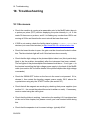
10. TROUBLESHOOTING
10.1 No muons
10.2 Computer Problems: Restarting SECI
10.3 Resetting the kicker
11.
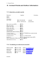
CONTACT POINTS AND FURTHER INFORMATION
11.1 Laboratory contact points
11.2
Contacting an instrument scientist
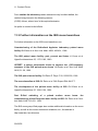
11.3 Further information on the ISIS muon beamlines
11.4 Local information
List of figures
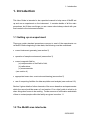
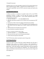
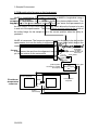
Figure 1. Layout of the ISIS muon beamlines.
Figure 2. Field and detector arrangements in the two MuSR geometries
Figure 3. MuSR detector numbering
Figure 4. The top of the Oxford Instruments cryostat
Figure 5. The front panel of the ITC5 temperature controller
Figure 6. The Orange cryostat
Figure 7. The flow cryostat centre stick.
Figure 8. Furnace connections
Figure 9. MuSR sample mounts
Figure 10. Range curve in the MuSR/EMU furnace
Figure 11. Frequency response in transverse fields
Figure 12. Effect of high longitudinal fields on asymmetry
Figure 13. Measurement of the muon beam spot size
Figure 14. Event rate as a function of slit setting
22/02/2005
1. Introduction
Figure 15.
Figure 16.
Figure 17.
Figure 18.
Figure 19.
Steering curve examples
Beamline power supply layout
Spin rotation by the separator seen in a single detector
Grouped data with and without dead time correction
Reference diagram for resetting the kicker
DEVA
kicker
separator
dipole
steering magnet
quadrupole
focusing magnet
MuSR
EMU
These components are unshielded
and are visible from the platform
above the beamlines
muon
production
target
proton beam
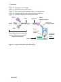
Figure 1. Layout of the ISIS muon beamlines.
22/02/2005
to neutron
production
target
1 - Introduction
1. Introduction
This User Guide is intended to be a practical manual to help users of MuSR set
up and run an experiment on the instrument. It contains details of all the main
procedures, but if there are things you are unsure about always check with your
local contact or the instrument scientist.
1.1 Setting up an experiment
There are certain standard procedures common to most of the experiments run
on MuSR. Before beginning to take data, the following must be considered:
• correct instrument geometry (see section 2)
• operation of sample environment (see section 3)
• correct magnetic field for
(a) compensation of the Earth’s field,
(b) calibrations,
(c) measurements
(see section 4)
• appropriate beam size, event rate and steering (see section 5)
• use of computing facilities for data acquisition and analysis (see sections 6-8)
Section 9 gives details of other elements of the muon beamline and spectrometer
which the user should be aware of, and section 10 is a brief guide to what to do
when things don’t seem to be working. Further sources of information and details
of how to contact people within the facility are given in section 11.
1.2 The MuSR area interlocks
22/02/2005
1. Introduction
1.2.1 Closing the area
The blocker which prevents muons entering the MuSR area can only be raised
once the area interlocks are complete. For this to happen:
1. Close the gate which allows access above the spectrometer on the top of the
MuSR platform, remove its key and insert into the key box to the right of the
lower area door. Turn the key clockwise.
2. Check that no-one is inside the MuSR area. Press the search button (situated
on the far side of the spectrometer) and close the area door and remove the
key from the lock (turning anticlockwise). Insert this key into the key box to the
right of the door, turning it clockwise.
3. The key box should now be full. Remove the bottom right hand key and insert it
into the green box to the right of the key box, turning it clockwise.
4. Check that the Helmholtz magnet interlock key below the blocker raise / lower
buttons is in the vertical position (see section 4.3).
5. The blocker can now be raised: press the red raise button and keep it pressed
until the blue area lights come on and the blocker has stopped moving.
1.2.2 Entering the area
To enter the MuSR area
1. If you require the main Helmholtz coil field to not be set to zero, check that the
key below the blocker raise / lower buttons is in the override (horizontal)
position (see section 4.3).
2. Lower the blocker by pressing and holding the green button. The area lights
come on once the blocker is down.
3. Remove the key from the green box by turning it anticlockwise, insert it into the
bottom right position on the key box and turn it clockwise.
4. Remove one of the keys (the two left-most keys on the top row are often the
easiest) from the key box and insert it into the door lock. Turn it anticlockwise.
The door can now by opened by removing the locking bolt.
5. If it is necessary to open the gate on the MuSR platform, remove a second key
from the key box and insert it into the gate lock, turning it clockwise.
22/02/2005
1 - Introduction
22/02/2005
2. The MuSR Spectrometer
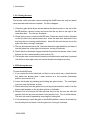
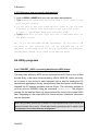
2. The MuSR spectrometer
Positrons from the decay of muons implanted into the sample under investigation
are detected using scintillation detectors. MuSR contains 64 such detectors,
each consisting of a piece of plastic scintillator joined by an acrylic light-guide to
a photomultiplier tube. The detectors are arranged in two arrays around the
sample position on a cylinder concentric with the coils of the main Helmholtz
magnet.
The detector arrays and Helmholtz coils can be rotated on their support platform
about a vertical axis. When the spectrometer is in longitudinal geometry, the
Helmholtz coils provide a field (of up to 2500 G) which is parallel to the initial
muon polarisation direction. Rotating the spectrometer through 900 in a
clockwise direction looking from above puts in into transverse geometry, in which
the Helmholtz coils provide a field which is perpendicular to the initial muon
polarisation direction. In this case, fields of up to about 600 G are useable,
limited by the frequency response caused by the finite width of the muon pulse
(see section 4.3.1).
magnets and detectors
magnet and detectors
µ+
sample
+
µ
sample
magnet and detectors
Transverse Field
Longitudinal Field
Figure 2. Field and detector arrangements in the two MuSR geometries
22/02/2005
2 .The MuSR Spectrometer
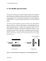
In the longitudinal case, one detector array is forward of the initial polarisation
direction, and one is backward. Looking upstream (i.e., anti-parallel to the muon
momentum, parallel to the initial polarisation direction), the detectors are
numbered as below.
Detector 1
Beam In
Detector 33
Figure 3. MuSR detector numbering
In order to form a longitudinal forward-backward grouping, detectors 33-64 are
summed to form the forward set, and detectors 1-32 summed for the backward
set.
In the transverse case, the two detector arrays are perpendicular to the initial
polarisation direction. A suitable way of grouping the detectors in this case is in
four groups of eight: top (17-24 + 49-56), bottom (1-8 + 33-40), forward (9-16 +
57-64) and backward (25-32 + 41-48). These sets can be analysed separately,
or further arranged into forward-backward sets (top-bottom, forward-backward).
MuSR can be rotated between transverse and longitudinal geometry in about 30
minutes. However, it is important that an instrument scientist be present
when the rotation is carried out: careless actions during the rotation can
damage the photomultiplier tubes or puncture the windows in the beam line or
dilution refrigerator.
22/02/2005
2. The MuSR Spectrometer
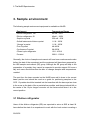
3. Sample environment
The following sample environment equipment is available on MuSR:
Equipment
Temperature Range
Dilution refrigerator, TBT
Dilution refrigerator, OI
Sorption cryostat
Oxford Instruments Variox cryostat
‘Orange’ cryostat
Flow Cryostat
Cryofurance Cryostat
Closed cycle refrigerator
Furnace
40 mK - 4.2 K
40mK – 300K
350 mK - 50 K
1.6 K - 300 K
1.6 K - 300 K
4K-400K
6K-600K
12 K - 400 K
300 K - 1000 K
Generally, the choice of sample environment will have been made several weeks
before the start of the experiment and the equipment will have been prepared by
the ISIS sample environment (SE) group. Although the SE group will help in the
preparation of cryostats, they cannot be expected to provide support 24 hours a
day and users should therefore be able to change samples and temperatures
unaided.
The spot from the laser mounted on the MuSR area wall is close to the correct
beam position and should be used as a guide for positioning samples in the
CCR. Cryostats should be inserted into the beamline with the laser spot as close
to the cross on the back of the cryostat tail as possible, and the spot should fall on
the centre of the 12-pin Jaeger connector on the furnace stick when it is in the
correct position.
3.1 Dilution refrigerator
Users of the dilution refrigerator (DR) are expected to arrive at ISIS at least 24
hours before the start of an experiment to work with the local contact mounting a
22/02/05
3. Sample Environment
sample and starting the precooling process. This takes place out of the beam
during the previous users’ beam time. Once the DR is prepared it has to be
lowered into the beam by a licensed crane driver.
3.2 Sorption cryostat
Users of the sorption cryostat are expected to arrive at ISIS at 24 hours before
the start of an experiment to work with the local contact mounting a sample and
starting the precooling process (to 4K). This takes place out of the beam during
the previous users’ beam time. Once the sorption cryostat is prepared it has to
be lowered into the beam by a licensed crane driver. There is a separate manual
describing the operation of the 3He sorption cryostat.
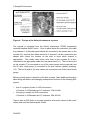
3.3 The Oxford Instruments Variox cryostat
The Oxford Instruments ‘Variox’ cryostat is a replacement for the MuSR Orange
cryostat, with faster cool-down time and lower He consumption rate. Its principles
of operation are very similar, with the exception that the Variox requires
continuous pumping to promote He flow through its capillary, whereas the orange
cryostat used the pressure inside the He bath to achieve this above 4.2K.
The cryostat will have been prepared off-beam by a member of the ISIS sample
environment team. It must be craned into place on the beam line only by a
licensed crane operator. Three spacers fit over each of the cryostat resting
points on the platform above the beamline to position the cryostat at the correct
height.
22/02/05
3. Sample Environment
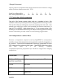
Figure 4. The top of the Oxford Instruments cryostat
The cryostat is controlled from the Oxford Instruments ITC503 temperature
controller labelled ‘MuSR Variox’. Once in place above the instrument, the cable
from channel 1 of the patch panel should be connected to the sensor port on the
cryostat (12), and that from either channel 2 or channel 3 can be connected to the
sample stick (check the number on the stick to know which channel is
appropriate). The needle valve motor drive lead on the cryostat (4) is also
connected to the appropriate cable from the patch panel (V1). The He return port
on the cryostat (7) is connected to one of the return panels on the cage wall, and
the 25 m3/hr rotary pump is connected to the port marked ‘capillary pumping’
(13). The He (9) and N2 (2) level meters are connected to the Oxford level metre
gauge.
Below is a brief guide to operation of the blue cryostat. More detailed information
about filling with helium and changing a sample can be found in the following RAL
reports:
•
•
Use of cryogenic liquids on ISIS instruments
J Chauhan, A V Belushkin and J Tomkinson, RAL-92-041
Changing a sample on ISIS instruments
J Chauhan, A V Belushkin and J Tomkinson RAL-93-006
There is also an ISIS video on cryostat operation; this can be viewed in the users’
coffee area near the Data Analysis Centre.
22/02/05
3. Sample Environment
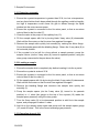
3.3.1 Removing a sample
1. Ensure the cryostat temperature is greater than 25 K; too low a temperature,
and any liquid helium that’s been pulled through the capillary could boil rapidly;
too high a temperature could cause He gas to diffuse through the Mylar
window into the outer vacuum space.
2. Ensure the cryostat is connected to the He return panel, or that a non-return
valve is fitted to the He outlet (7).
3. Close the valve to the pump on the capillary line (13).
4. Fill the sample space with He by turning black 3-way valve (8) downwards.
Wait until the flow meter on the He return line registers flow again.
5. Remove the sample stick quickly but smoothly by undoing the Klein flange.
Cover the sample space with the blanking flange. Return the 3-way valve (8) to
its horizontal position.
6. If the cryostat is to be left for a time without a sample present, pump the
sample volume (via the 3-way valve (8), turned to upwards position, using the
rotary pump connected to the port above the valve).
3.3.2 Loading a sample
1. Ensure the sample stick is completely dry before inserting it into the cryostat.
2. Ensure the cryostat is at about 25 K.
3. Ensure the cryostat is connected to the He return panel, or that a non-return
valve is fitted to the He outlet (7).
4. Fill the sample space with He by turning the black 3-way valve (8) downwards.
Wait until the flow meter on the He return line registers flow again.
5. Remove the blanking flange and introduce the sample stick quickly but
smoothly (3).
6. Pump the sample space (via the 3-way valve (8), turned to its upwards
position) to ~1 mbar (the gauge on the top of the cryostat (10) reads the
sample space pressure) using the rotary pump.
7. Turn the 3-way valve (8) to its downwards position to add He to the sample
space, and pump again to about 1 mbar.
8. Add He to the sample space again and pump until the sample space gauge
(10) reads 20 mbar. This is the correct exchange gas pressure.
3.3.3 Operation above 4.2 K
22/02/05
3. Sample Environment
Operation above 4.2 K is fully automatic once the 25 m3/hr pump has been set to
pump He gas through the capillary. Set-points can be entered using the settemp
command in OpenGENIE, and the ITC503 controls the heater and needle valve
settings.
3.3.4 Operation below 4.2 K
A different procedure is necessary for operation below 4.2K, as the ITC503
temperature controller is unable to set the gas flow through the cryostat
automatically for these temperatures. To get to base temperature (about 1.6K)
use the following procedure:
1. Issue the command blue_lt in the OpenGENIE window.
2. Manually check that the set-point in the ITC503 is zero by pressing the ‘SET’
button.
3. Connect the 0-1000 cm3/min flow gauge to the Rootes pump exhaust.
4. Manually adjust the gas flow on the ITC503 until the pump exhaust flow rate is
about 450 cm3/min (you need to be in ‘LOCAL’ mode on the ITC503 to do
this).
5. The temperature should rapidly drop to below 2K.
6. Enter set-points as normal up to about 5K.
To return to automatic operation above 4.2K
1. Issue the command blue_ht in OpenGENIE window
2. Disconnect the flow meter from the Rootes pump exhaust.
3. Set the desired temperature within MCS.
The ITC503 should go back to automatic control of the gas flow.
3.3.5 Filling with Helium
The time for which a helium fill will last is greatly dependant upon the type of
experiment being carried out. Sustained running at high temperatures or
repeatedly cycling between high and low temperatures can require a fill every
twelve hours. At the other extreme, a helium fill can last for well over twenty-four
hours if running at a near constant low temperature. As a general guide, the
helium level should be checked at least once every twelve hours (don’t forget to fill
with nitrogen too).
22/02/05
3. Sample Environment
The following procedure should be followed to fill the cryostat. Users should note
that two people are required. Use the flexible transfer tube on the side of the
MuSR platform.
1. Set the He level gauge for high readout rate.
2. Open the by-pass valve on the He return line.
3. Vent the helium storage dewar by opening the red valve. Open the top valve
on the dewar then close both red and green valves.
4. Slowly lower the longer end of the transfer line into the helium storage dewar.
The other end of the transfer line will require support. The fitting on top of the
storage dewar should be tightened to prevent gas escaping.
5. Helium gas should immediately begin exhausting from the transfer line. After
approximately one minute cold gas will be felt and a short while later a plume
will form.
6. Once a plume is observed quickly insert the transfer line into the helium fill port
on the cryostat (normally closed by a brass plug). Note that if refilling with
helium the transfer line should only be pushed approximately halfway into the
cryostat dewar.
7. Helium transfer should now take place, the process taking a few minutes (for
a refill).
8. During the transfer an over-pressure must be maintained in the helium storage
dewar using a He gas line or bladder attached to the red port.
9. When the helium level gauge measures 100% stop the transfer by releasing
the pressure in the storage dewar, typically by removing the gas line / bladder
and opening the red valve. Remove the transfer line from the cryostat and
replace the brass plug, ensuring it has been fully tightened (the fitting may
require heating). Remove the transfer line from the dewar and open the green
valve.
10. Leave the helium storage dewar with both the top valve and the red valve shut
and the green valve open.
11. Switch the helium level gauge to low readout rate.
12. When the He recovery flow has returned to less than 10 l/min close the He
recovery by-pass valve.
3.3.6 The Oxford ITC503 Temperature Controller
22/02/05
3. Sample Environment
DISPLAY
1
HOLD
2
SWEEP
3
SENSOR
SWEEP
PROG
PROP
INT
DERIV SET
RUN/PROG
HEATER
GAS
FLOW
1
PID
CNTRL
2
REM
3
SENSOR
ADJUST POWER
LOCK
RAISE
LOCAL
AUTO
MAN
AUTO
AUTO
LOC/REM
LOWER
POWER
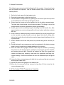
Figure 5. The front panel of the ITC5 temperature controller
A diagram of the front panel of the ITC503 is shown below. Two types of
interaction with the controller are possible: inspecting the present settings while
running the controller in automatic mode, and switching to manual control to adjust
parameters.
Inspecting the controller (automatic operation)
To guard against inadvertently altering settings, the user should ensure the
controller is in remote mode (i.e. the remote light is on) before inspecting any
parameter. Pressing the 'LOC/REM' button toggles the controller between local
and remote modes of operation.
Requirement
Action
View temperature of sensor Press the ‘SENSOR’ button until the LED
1, 2 or 3
corresponding to the particular sensor is alight.
View current set temperature Press the ‘SET’ button.
View current heater voltage
Press the ‘AUTO’ button under ‘Heater’.
After checking the parameter ensure that the controller is still in the required
mode of operation, usually with the heater in automatic mode.
Manually adjusting parameters
Switch the controller to the local mode of operation by pressing the 'LOC/REM'
button. Note that SECI will periodically return the controller to the remote mode.
22/02/05
3. Sample Environment
Requirement
Action
Adjusting the set temperature
Press the ‘SET’ button with either the ‘RAISE’
or ‘LOWER’ buttons under ‘ADJUST’.
Adjusting the heater voltage
Press the ‘MAN’ button under ‘Heater’
simultaneously with either the ‘RAISE’ or
‘LOWER’ buttons under ‘ADJUST’. The voltage
can be read. Note that the heater sensor is
always number one.
Adjusting Gas Flow
Press the ‘AUTO GAS’ button simultaneously
with either the ‘RAISE’ or ‘LOWER’ buttons
under ‘ADJUST’.
Adjusting PID’s
Press either ‘P’, ‘I’ or ‘D’ button simultaneously
with either the ‘RAISE’ or ‘LOWER’ buttons
under ‘ADJUST’.
22/02/05
3. Sample Environment
3.4 Orange cryostat
Figure 6. The Orange cryostat
Operation of the orange cryostat is very similar to that described above for the
Oxford Instruments Variox. The OC is controlled by the ITC5 temperature
controller labelled ‘MuSR orange’ on the platform above the spectrometer.
22/02/05
3. Sample Environment
3.4.1 Removing a sample
Instructions are as for the Variox – the black three-way valve on the top of the
Variox has the same operation as the blue 3-way ‘Hoke’ valve on the top of the
orange cryostat.
3.4.2 Loading a sample
Again, the procedure is the same as for the Variox cryostat.
3.4.3 Cooling the cryostat to 4.2 K
Operation is similar to the Variox in principle; however, the gas flow through the
cryostat is controlled manually using the ‘cold’ valve (valve 4 in the orange
cryostat diagram) and the ‘warm’ valve (valve 6). The cold valve controls a needle
valve which allows liquid helium from the main reservoir into the annular space via
a capillary and heat exchanger. To close the cold valve it should be turned
clockwise. Be careful not to over-tighten it, otherwise the needle may be
damaged.
1. Open the cold valve (rotate it between half and one turn anti-clockwise from
when it first ‘bites’).
2. Open the warm valve until the He flow rate is at maximum on the He return line
meter (10 l/min).
3. Wait for the cryostat to cool to the desired temperature.
4. Close the warm valve until the He flow rate is 4-5 l/min.
3.4.4 Cooling the cryostat below 4.2K
This requires the He brought through the needle valve to be pumped using the
large ‘Roots’ pump. The cryostat temperature must be below 50 K before
pumping starts.
1. Connect the Roots pump to the He pumping valve (valve 3) of the cryostat.
2. Close the cryostat cold and warm valves fully.
22/02/05
3. Sample Environment
3. Make sure the cryostat valve 3 is closed. Disconnect the flow meter from the
Roots pump outlet if one is attached. Turn the Roots pump on (press both
green buttons) and open the big isolation valve on the pump to evacuate the
line up to the cryostat. Wait until the gauges on the pump read zero.
4. Slowly open valve 3 of the cryostat. Wait for a few minutes, then reconnect the
flow meter to the Roots pump outlet line. Open the fine control of the cold valve
very slightly, until the pump flow meter is reading maximum.
5. When the cryostat has reached the required temperature, close the cold valve
until the pump flow meter is reading <4 l/min (this may mean winding the valve
control until it is fully closed).
3.4.5 Filling with Helium
Again, this is very similar to the Variox cryostat. A different He level gauge is
used for the orange cryostat – you’ll need to switch this on before filling, and to
turn it off afterwards. You need to open the depressurising valve on the He return
line on the cryostat (valve 8) before filling – remember to close it again
afterwards.
3.4.6 Care of the cryostat when not in use
The cryostat can be left in its support frame, either on the MuSR platform or at
ground level, when not immediately required. In this case, users should leave the
cold and warm valves open a very slight amount to allow a small flow through the
cryostat; this reduces the chance of the cryostat blocking, but does not use large
amounts of helium. Users should still remember to check the cryogen
levels once every twelve hours and refill as required.
3.4.7 Additional notes
• At low temperatures, the exchange gas in the sample volume may have
condensed, leading to poor thermal contact to the annular space. The exchange
gas pressure can be monitored using the meter on the small rotary pump (with the
pump valve closed, and the blue Hoke valve turned upwards). If the pressure has
dropped, add more gas by turning the Hoke valve to its downwards position for
an instant, and then pumping the sample space to the required pressure.
• If oscillations in the temperature of the cryostat are observed, the exchange
gas pressure may be too high. Try pumping the exchange gas to 5-10 mbar.
22/02/05
3. Sample Environment
• When cooling, the He flow rate through the return line should be controlled by
the warm valve setting. If opening the warm valve a small amount doesn’t
increase the flow rate, open the cold valve until the rate increases and then close
the warm valve to achieve the required rate.
• When the cryostat is at the required temperature, the He flow rate should be
reduced to about 4-5 l/min. But this rate should be monitored for the first hour or
so after cooling as it will be affected by any liquid helium which has entered the
annular space. The flow rate may change as this liquid boils off and may become
too low when the annular space no longer contains liquid.
• At very low temperatures, an offset between the sample and cryostat
thermometers can be expected owing to condensation of the exchange gas in the
sample space.
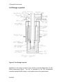
3.5 Flow Cryostat
The Flow crystats are controlled using an ITC5. The temperature range is 4 to
400K for the normal flow cryostat and 6K-600K for the cryofurnace flow cryostat.
3.5.1 Sample holder
This cryostat can use the same sample holders as the EMu “Blue” cryostat:
37mm square with hole spacing 30mm. The internal diameter of the cryostat is
43mm.
Length scale 19mm
70 mm
Locating pin
on top flange
Muons
615mm
Angular
scale 0 deg
Locking screws
Side view
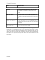
Figure 7. The flow cryostat centre stick.
22/02/05
Sample
End view
3. Sample Environment
With the standard blade and sample holder, the length from the bottom of the
copper block to the sample centre is 70mm and the top adjustment should be set
to 19mm. If a non standard sample mount differs from 70mm, adjust the top scale
by the same amount.
For the standard blade, set the angle to 0 degrees. The muon arrival direction is
in line with the locating pin on the top flange and the sample plate should normally
be perpendicular to this. You can rotate the sample relative to the beam if
required by your experiment, either now or when in the cryostat.
3.5.2 Installation
The cryostat fits into a support cage. This cage should be mounted above dizital
and the cryostat lowered into the support cage (use of the crane requires a
crane drivers license). Install it with the transfer tube connection in the
“downstream” direction. The locating pin on the top flange will be towards the
beam.
Use the appropriate ITC5 temperature controller for the cryostat and connect
through the patch panel.
Start pumping the OVC using a turbo pump.
3.5.3 Connections
•
•
•
•
Cryostat sample space port should be connected to a T-connector which is
connected to He gas, gauge and rotarty pump.
Cryostat heater/thermometer to ITC channel 1, the stick thermometer to ITC
channel 2 (stick A) or 3 (stick B) and the transfer tube needle valve to ITC Aux.
Out, through the patch panel
Transfer tube gas outlet (at the top of the dewar leg) to the pumping box via a
long plastic tube
Connect using the switch box.
22/02/05
3. Sample Environment
3.5.4 Inserting the stick
The sample can be changed when the cryostat is cold, but heat it up to >25K first.
• Let the sample space up to 1 atm with helium.
• Insert the stick: the pin on the stick flange should locate into the hole in the
flange on the cryostat.
• Pump the sample space, purge two or three times with helium, and set the
exchange gas pressure to 15 mbar.
3.5.5 Cooling
•
•
•
•
•
Check that the PTFE sealing washer is present on the cryostat end of the
transfer tube.
Connect the needle valve cable. Turn the ITC5 on. This initialises the valve.
Open the needle valve fully: press and hold “Gas Auto” and then press
“Raise”. Check it stays in Manual (light off).
Check with your local contact that the dewar has the helium level probe
installed.
Insert the leg of the transfer tube in the dewar. Be very careful not to bend
the transfer tube. In practice the tube will need to be almost fully inserted into
the dewar before the transfer tube can be inserted into the cryostat. Reduce
pressure in the dewar as required with the red valve.
• Put the transfer tube into the cryostat and tighten the locking nut. Turn on the
diaphragm pump. Open the valve on the pumping box. There should be a very
small flow.
• After about 5 minutes the flow should increase as liquid reaches the cryostat,
and the temperature will start to fall.
• The Green valve on the dewar should be open and the Red valve closed
during operation.
If the cryostat is still not cooling after 20 minutes, the tube may be blocked with ice
or solid air:
• Remove the transfer tube from the cryostat and dewar.
• Warm both ends with the hot air gun.
• Blow clean helium gas through it – use a piece of rubber tube over the
cryostat end.
3.5.6 Removing
22/02/05
3. Sample Environment
•
•
•
•
•
•
•
Warm the cryostat to 25K or above.
Ensure the needle valve on the transfer tube is open (set the ITC5 to Local,
then press Gas Flow and Raise) then shut the valve on the pumping box. The
pressure should rise rapidly to 1 atm. If it doesn’t, check with your local
contact.
The transfer line can then be removed. Be careful not to bend either of the
legs. If the cryostat will be used again during the experiment the transfer line
may be left in the dewar with the needle valve closed. Be sure to fit the
protective tube over the free end of the transfer line.
Unplug all the electrical leads from the cryostat. Close the sample space tap
and disconnect the sample space pumping line.
Close the OVC value and switch off and disconnect the turbo pump.
The cryostat and lift it out.
Remove the frame
22/02/05
3. Sample Environment
3.6 Closed-cycle refrigerator (CCR)
The CCR is controlled using the Eurotherm TC820 controller in the rack in the
MuSR area. Check that both data switches (in the MuSR area and in the back of
the MuSR cabin) are at the CCR position.
Users will need to know how to change the sample in the CCR. In preparation for
a sample change the temperature should be set to 300K and the compressor
turned off. Once the CCR has reached a reasonably high temperature (>270 K)
the following procedure can be carried out to remove the sample:
• Close the large isolation valve on the top of the pump
• Switch off the pump
• Open the vent valves to vent the pump and CCR
• Swing the CCR out from between the magnet faces
• Remove the CCR tails and unscrew the sample plate from the copper block
TAKE CARE NOT TO BEND THE RhFe THERMOMETER LEADS
After mounting a new sample, close and restart the CCR in the following way:
• Dry the CCR, heat shield and outer tail (use a heat gun, but be careful not to
heat the thermal fuse). Replace the tails, checking that the windows are
aligned and facing the muon beam pipe window.
• Swing the CCR back into place taking care not to knock the calibration coils.
• Check the vent valves are closed.
• Start the vacuum pump and switch on the Pirani gauge.
• Slowly open the large pump isolation valve.
• When the Pirani gauge reads <10-1 Torr the Penning gauge automatically
•
switches on.
Below 5x10-3 Torr the compressor may be switched on by turning the switch
on the front the central compressor (outside the area) from 0 to 1.
The compressor must be left on for all sample temperatures, including
those above room temperature.
There is a thermal fuse on the heater lead inside the CCR to prevent excessive
heating. Users can check that the heater is working by heating to slightly above
room temperature before starting to cool. If the heater does not work then check
the Eurotherm trip.
22/02/05
3. Sample Environment
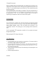
3.7 Furnace
The muon furnace is designed to allow µSR experiments to be carried out on the
EMU and MuSR spectrometers (with MuSR in either longitudinal or transverse
orientation) at temperatures from room temperature up to 1000 K.
It consists of an outer vacuum jacket with a thin (30 µm) titanium window to allow
muon entry, into which a centre stick is inserted which holds the sample and
heating element. The sample temperature is monitored by a thermocouple
sensor mounted on the sample plate, and controlled by a Eurotherm temperature
controller; this in turn is monitored and controlled from MCS. The outer body of
the furnace is cooled by water flowing through external pipes and around the
muon entry window. Two heat shields (also 30 µm Ti) between the entry window
and the sample position also reduce heating effects on the furnace window. Zero
field should be reset after the furnace support is mounted.
3.7.1 Sample mounting
The furnace centre stick allows samples up to 40 mm x 40 mm to be mounted,
and the Ti mounting plate is drilled to allow sample holders of the size and shape
used on the EMU blue cryostat to be fixed (M3 screw holes arranged in a square
with 30 mm between their centres). Titanium sample holders are available for
use with powdered samples. These consist of a Ti plate with a depression into
which a powder can be packed and over which a thin Ti window can be fixed
using a clamping ring. Ti screws and thin Ta wire are available for attaching a
sample holder to the mounting plate. Ti produces a negligible depolarisation of
the muon signal at furnace temperatures and so is suitable for use as a mask
material. Thick windows in front of a sample should be avoided as the four Ti
foils (including the one on the sample mount) reduce the muon penetration to less
than 70 mg.cm-2; a range curve a taken in the furnace is given in figure 8, section
3.8.
It should be noted that Al and Ag sample holders are NOT suitable for use in
the furnace owing to the low melting point of Al; similarly, users should consider
whether their sample has a melting or decomposition temperature within the
reach of the furnace and take suitable precautions!
22/02/05
3. Sample Environment
3.7.2 Mounting the furnace on the instrument
MuSR in Longitudinal: The furnace is mounted on MuSR in longitudinal using a
heater
(mains required)
4-pin
support frame
which is fixed to the
frame holding the photomultiplier tubes. The
power
0123456
output flow
base part of the furnace 9V
support
is attached to the four struts fixed permanently to
supply
in
the PMT frame; on top of this is bolted a trolley which allows the furnace to be slid
in and out of the spectrometer. The furnace flange must be bolted to the inside of
the trolley flange for the sample to be in the correct position when the trolley is
pushed in.
MuSR in transverse: The furnace is again mounted on its trolley to be slid into the
spectrometer; but now the trolley is supported by a larger
frame which bolts to the
water out
rotating table supporting DIZITAL.
flowmeter
12-pin
furnace
In both cases, the spot from the alignment laser should fall Jaeger
in the centreon
ofwater
the 12return line
pin Jaeger socket on the centre stick.
2-pin yellow
thermo
couple out
water
(match yellow
connector to yellow
box inputs)
2-way split
red
thermocouple
box
(mains required)
(mains required)
Eurotherm
temperature
controller
9V DC
sensor
(Lemo
connectors)
22/02/05
to acquisition
computer
RS232
sensor
3. Sample Environment
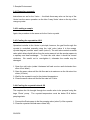
Figure 8. Furnace connections
3.7.3 Connections
Once the furnace body, with centre stick in place, has been mounted on the
instrument connections as shown in the diagram below are made.
1. The lead from the sample thermocouple (thermocouple B) is connected via a
red lead to the yellow terminal of the red thermocouple box. A two-way splitter
is connected to the white output terminal of the box to feed two leads which
attach to the sensor inputs on the Eurotherm controller via Lemo connectors.
22/02/05
3. Sample Environment
2. The 12-pin Jaeger connector on the centre stick is connected to the 4-pin
output on the heater power box.
3. The 9V DC output of the Eurotherm is connected to the 9V input on the heater
box via Lemo connectors.
4. The flowmeter signal wire is connected to the flow input on the heater box via a
Lemo connector.
5. The RS232 link on the Eurotherm is connected to the RS232 cable in the area
(use the one normally devoted to the CCR Eurotherm). Check that the two
sample environment data switches are in the CCR position.
6. The two cooling water hoses are connected to the two tubes on the furnace
body (it doesn’t matter which way round). The hose with the flow sensor must
then be connected to the water return socket on the area wall, and the other
hose connected to the water output socket. Don’t forget to turn the cooling
water on - there are two taps, one on the feed line and one on the return line.
7. The furnace pumping port on the centre stick is connected to the rotary/turbo
pump set in the area via a 4-way cross-piece which also allows connection of
a pressure gauge and a valve to admit He exchange gas. It is useful to ensure
that there is a valve capable of isolating the furnace in place between the
furnace and the cross-piece. The pump set used should be one reserved for a
furnace to avoid contaminating a clean set.
The flow sensor on the water return line is designed to cut off the heater power to
the furnace if the flow falls to too low a level. The LED on the heater box by the
flow input goes out if the heater has been tripped in this way.
22/02/05
3. Sample Environment
3.7.4 Eurotherm set-up
Normally, a dedicated Eurotherm is provided which will be already set up for
furnace use. However, in the event of a CCR Eurotherm having to be used to
control the furnace, please ask your local contact to configure it for use with
thermocouple sensors. For full details of operating a Eurotherm, see ‘The Users
Guide to the Temperature Controllers’ by H.M. Shah (copies are in the filing
cabinet in the EMU cabin).
3.7.5 Controlling the furnace
Exchange gas within the furnace vacuum jacket is necessary to allow control over
the low temperature part of the furnace range (up to about 200 oC). The
rotary/turbo pump set connected to the furnace pumping port can be valved off
once a good vacuum has been reached and 20 mbar or so of He gas introduced
into the furnace body. This can then be pumped out for high-temperature
operation.
There are six different heater power settings (and an off, ‘0’, setting) on the heater
box. The table below shows the heater settings, PID and exchange gas values
required at different temperatures.
Max.
working
Temperature
°C
Eurotherm
Heater
Power
(%)
Heater box
voltage
setting
P
(%)
I
(s)
D
(s)
Exch
ange
gas
100
25
2
0.8
70
14
Yes
200
50
2
0.7
70
14
Yes
300
100
2
2.7
125
25
No
400
25
3
4.9
125
25
No
500
100
3
6.2
105
21
No
600
50
4
16
55
11
No
700
50
5
16
35
7
No
These settings have been optimised to achieve the best possible stability. Users
wishing to scan a temperature range on a script may be able to find a
compromise in the settings that will still achieve reasonable stability, but will allow
unattended operation over an extended temperature range. However, please
22/02/05
3. Sample Environment
note the maximum temperature that can be reached for each heater box voltage
setting (Eurotherm heater power set at 100%):
Heater box voltage setting
Max. working temperature (°C)
1
190
2
380
3
510
4
640
5
700
6
700
3.7.6 Typical data collection parameters
The wall of the furnace vacuum jacket acts as a degrader in front of the
scintillation detectors, preventing the lowest energy positrons from being counted.
This has the effect of reducing the count rate (requiring the beam slits to be
opened more widely than normal) and increasing the maximum asymmetry (to
close to 27% on MuSR). Alpha values close to 1.5 are common owing to the
shielding of the backward detectors by the sample mounting plate and heating
element. Check with your local contact for correct steering magnet values.
3.8 Temperature control files
Whenever a temperature set-point is sent by OpenGENIE to a temperature
controller, various other parameters are also passed to enable the temperature to
be controlled. These include the appropriate Proportional, Integral and Derivative
(PID) values and the maximum heater power. OpenGENIE reads these values
from
files
which
sit
in
the
directory
c:\labview
modules\mkscript3\muon_temperature.tpar. This file is changed when changing
configurations.
Column label
function
TLOW and THIGH (or
MINTEMP, MAXTEMP)
specify a temperature range for given PID values
CYCLE
Max Power
PROP
proportional value
INT
integral value
22/02/05
3. Sample Environment
DER
derivative value
ACCUR
the temperature range around the set point within
which MCS will consider the temperature to be
stable
WAIT (or TWAIT)
the length of time (mins) that the temperature must
be within the accuracy band before MCS will start a
run
TMOUT (or TIMEOUT)
the time after which, even if the temperature has not
stabilised within the accuracy band, MCS will start a
run anyway
MAXI (fridge only)
controls the heater power range
Occasionally, it is necessary to alter the PID values that OpenGENIE is using.
This can be done by editing the appropriate muon_temperature.tpar file (use
notpad) and then re-sending the temperature set-point (for Eurotherm/ITC5).
Information in the .tpar files is arranged as a table, with columns labelled as in the
table above.
22/02/05
3. Sample Environment
3.9 Sample mounts
Figure 9. MuSR sample mounts
22/02/05
3. Sample Environment
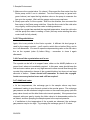
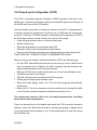
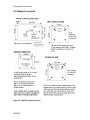
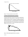
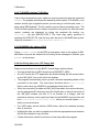
3.10 Range curve
The muons in the beam hit the front surface of the sample at about 0.25 c (3.0
MeV) and are then slowed by interactions within the material before stopping.
The implantation energy of the muons results in them passing through several
hundred microns of material before they come to rest. The actual amount of
material traversed and the width of the muon distribution depend upon the
material’s density - as a rough guide the muon range is roughly 100 mg.cm-2 of
material i.e. about 1 mm of water, 500 µm of silicon, etc.
Figure 8 below shows the diamagnetic asymmetry (in a 20 G transverse field) as
thin titanium foils (thickness about 25µm) are added in front of a thick quartz plate
mounted in the MuSR/EMU furnace. Initially a low asymmetry is recorded as all
muons are stopped in the quartz where there is an appreciable muonium fraction.
Adding more than four titanium foils causes the asymmetry to rise as an
increasing proportion of the muons are stopped in the metal (in which all muons
thermalise into a diamagnetic state). Full asymmetry is obtained when at least
ten foils have been added.
Range Curve, Furnace
Ti foils (11.2mg/cm 2) in front of Quartz plate
30
Asymmetry (%)
25
20
15
10
5
0
0
2
4
6
8
10
Number of foils
Figure 10. Range curve in the MuSR/EMU furnace
It should be noted that in the dilution fridge additional windows in the cryostat tails
reduce the muons’ energy significantly before they reach the sample. Any
material placed over samples for the fridge should be very thin indeed (10 µm
thick silver is used for heat shields) otherwise the muons may not reach the
sample.
22/02/05
3. Sample Environment
Samples for µSR experiments should be appreciably thicker than the average
muon stopping distance. When thin samples are used, sheets of metal or plastic
should be added in front of the sample to maximise the signal from the sample
and to prevent the muons from passing all the way through. The decision to use
either metal or plastic as the degrader will generally depend upon the nature of
the sample being studied and the need to create a contrast between the sample
and degrader. For samples having a missing fraction, metal is the most
appropriate choice (pre-cut 30 µm-thick titanium sheets are available for this
purpose) while, conversely, a plastic degrader is ideal for metallic samples.
22/02/05
3. Sample Environment
4. Magnetic fields
4.1 Zero field compensation
Three pairs of orthogonal coils mounted around the sample position are used to
cancel the earth's magnetic field. They are powered from the three Iso-tect power
supply units (labelled L V and T) in the electronics rack inside the MuSR area.
The field is measured using a triple-axis fluxgate magnetometer mounted just
below the beamline window and is used to control the currents in the coils. A
second probe can be fixed at the sample position and used to check the zero
setting – read this on the display with the unit in the rack.
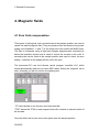
The Instrument PC runs the Labview control program “zerofield v5.vi” which
should automatically load and run when SECI starts. Select the “magnets” tab to
see it. Normally you will not need to do anything here.
“F0” tells Labview to use the auto zero field controller.
“TF20” selects the TF20 or main magnet returns the currents to manual control of
the currents.
Once the field is set to zero remove the probe from the sample position.
22/02/05
4. Magnetic Fields
If varying the current, on the vi, does not change the field at the sample position or
the message “current overload” appears on the PC, check that the coils have
been reconnected to the box on the fence between MuSR and EMU. If the field
readings remain fixed at about 5000 mG (their maximum) check that neither the
T20 coils nor the main Helmholtz coils are on.
The zero field calibration is different for longitudinal vs. transverse setups: change
over by using “Go To Longitudinal” or “Go To Transverse” buttons.
4.2 Calibration field
When working in longitudinal geometry it is necessary to start each section of
runs (after a sample change or change from CCR to cryostat for example) with a
calibration measurement in a transverse field of approximately 20 gauss. These
measurements are usually quite short (<5 Mevents) and are often referred to as
"T20" runs. Two small coils, which hang either side of the sample, are used to
provide a small transverse field. They are powered by a Gossen power supply
and controlled by the computer through OpenGENIE with the command TF20.
4.3 Applied fields
Magnetic fields are provided using the large Helmholtz coils powered by the
Danfysik PSU. This is controlled by MCS via a GPIB interface. The maximum
field available on MuSR is 2500 G. The Danfysik is operated as follows:
•
Type lf0 in OpenGENIE; this sets the magnet device to the Danfysik PSU.
Set fields using the command Setmag x. A read-out of the field is given on the
computer screen in the "MAGNET" window. If this is not successful then check
interlocks on front panel of magnet power supply.
Whenever the beam blocker is lowered the field generated by the Danfysik is
automatically set to zero. It is possible to over-ride this process by carrying out
the following procedure:
22/02/05
4. Magnetic Fields
•
Turn the key on the panel by the entrance to the experimental area to "override" before lowering the blocker
•
Open and close up the area as usual, but return the over-ride key to its original
position before raising the blocker
•
Check there are no red lights illuminated on the Danfysik power supply
If the power supply trips at any time it can usually be restored by reseting the
interlocks on the front panel. If this is not successful check the trip switches (see
section 9.1)
After selecting a new magnet device, always check that the field set via
OpenGENIE has been accepted by the power supply.
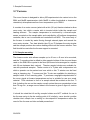
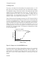
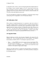
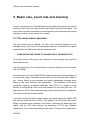
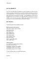
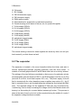
4.3.1 Effects of the finite muon pulse width on useable transverse fields
At ISIS the muons are produced in short pulses (about 80 ns wide at half height)
and the approximation is usually made that an average arrival time near the
centre of the muon pulse can be used as time-zero. This is adequate if the timescale of the evolution of the muon polarisation is long compared with the width of
the muon pulse but leads to difficulties in cases where the evolution is rapid. The
effect is seen clearly by considering a transverse field experiment performed at a
succession of magnetic fields. At low precession frequencies the polarisation is
seen with full asymmetry. As the frequency increases there is an appreciable
phase difference developed between muons from the beginning and end of the
pulse and the observed asymmetry falls. This is seen in the plot below, produced
from the precession of muonium in quartz in low transverse fields (data taken on
EMU, although the MuSR response is the same). Even though MuSR will allow
fields of up to 2000 G to be applied when in transverse orientation, the low
asymmetry limits the useable field to about 600 G (8 MHz).
22/02/05
4. Magnetic Fields
Frequency response of the µSR signal
9
Asymmetry (%)
8
7
6
5
4
3
2
1
0
0
2
4
6
8
10
12
Frequency (MHz)
Figure 11. Frequency response in transverse fields
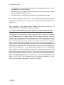
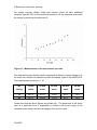
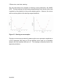
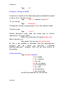
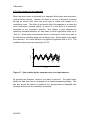
4.3.2 Effects of high longitudinal fields on asymmetry
The asymmetry measured for a large silver plate, mounted in the MuSR CCR, in
longitudinal magnetic fields up to 0.25 T, is shown below. As the field is
increased there is a small but gradual fall-off in the measured asymmetry, with
roughly a 3% reduction at 0.25 T. This change is an artefact that is probably a
result of a shift in the value of α caused by the interaction of the magnetic field
with both the decay positrons and the photomultipler tubes. Experimental data
can be corrected for the effect; however, the precise form of the curve seems to
depend on the initial value of α, and you are advised to perform your own
calibration and not rely on the curve below.
24.6
asymmetry
24.4
24.2
24.0
23.8
23.6
0
500
1000
1500
2000
field (G)
Figure 12. Effect of high longitudinal fields on asymmetry
22/02/05
4. Magnetic Fields
22/02/05
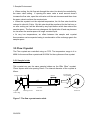
5. Beam size, event rate, steering
5. Beam size, event rate and steering
A set of collimation slits in the MuSR beamline just after the kicker can be used to
control the size of the muon spot and the rate at which muons hit the sample. The
muon beam can also be steered by small amounts in the horizontal and vertical
directions to allow it to be centred on a sample.
5.1 The muon beam spot size
The muon beam spot is elliptical. Its size in the horizontal direction can be
changed using a set of slits in the beampipe which are controlled from a panel
located behind the EMU area under the mezzanine floor.
CARE SHOULD BE TAKEN TO CHANGE ONLY THE MuSR SLITS
As a guide, set the x-slit equal to the x dimension of the sample, then check the
data collection rate.
The beam spot size in the vertical direction cannot be altered, and is of the order
of 8 mm FWHM.
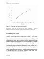
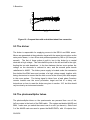
The beam spot size in the MuSR CCR has been measured for various settings of
the beam slits using a haematite sample with a 20 mm diameter silver mask on
top. Muons falling on the haematite are rapidly depolarised, whereas those
falling on the silver maintain their polarisation. The amplitude of the muon
precession signal in an applied transverse field (20 G) is a measure of the
fraction of muons falling on the silver and therefore of the muon spot size. Full
asymmetry (of 25.9%) was measured using a plain silver plate with no haematite.
The results are shown in the plot below.
It should be noted that these measurements were performed in the MuSR CCR
with its heat shield and tails in place. The window in the CCR tails (80µm-thick
Mylar) introduces some scattering of the beam, increasing the beam spot size
slightly: with the CCR tails removed, an asymmetry of 3.7% was obtained,
equivalent to 16% of the muons falling on the mask. The spot size is larger still in
22/02/05
5. Beam size, event rate, steering
the orange cryostat, dilution fridge and furnace, which all have additional
windows: typically 30% of the muons fall outside a 20 mm diameter area inside
the orange cryostat with the slits set to 8.
Figure 13. Measurement of the muon beam spot size
The table below gives similar results, expressed as fraction of beam falling on to
the mask, as a function of mask size for two slit settings, again in the MuSR CCR.
The measurement errors are +/- 1%.
slit
setting
10 mm
mask
20 mm
mask
25 mm
mask
29 mm
mask
38 mm
mask
12
60.7%
20.1%
12.4%
8.2%
< 4%
20
63.7%
25.6%
15.6%
8.7%
< 4%
Please note that the above figures are guides only. The actual size of the muon
spot at a particular time is dependent on factors such as the tuning of the
extracted proton beam, and can vary slightly from cycle to cycle.
22/02/05
5. Beam size, event rate, steering
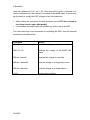
5.2 The event rate
In addition to controlling the muon spot size, the slits can be used to regulate the
event rate and thereby control the distortion at the start of histograms due to
detector dead time effects. Because various parts of the detector have
limitations on the speed with which they can respond there is a dead time, τ d ,
after each event during which further positron decays are missed. The effect of
this dead time can be modelled and the reduced rate observed in the experiment,
rob , is found to be related to the true rate, r , by the expression rob = r / (1 + rτ d ) .
Although the effect is particularly evident at high event rates, some distortion is
always present. Users should therefore always consider using the facilities
provided by both UDA and RUMDA to correct for this effect when analysing data.
The effects of deadtime on data are shown in figure 16 of section 9.3.
Rate must be kept below 55MeV/hr as this will give DAE2 more hits per frame
than it can cope with.
The graph below shows the event rate as a function of slit width for a large silver
plate mounted on the MuSR CCR with the 10 mm muon production target in use
and with ISIS running at about 170 µA. The main curve was taken without the
CCR tails in place - addition of the tails reduces the event rate slightly (point
shown as a cross) and also slightly increases the maximum asymmetry (this
effect is greatest in the furnace, where the event rate is two thirds of that in the
CCR and the asymmetry is typically a couple of percent higher).
22/02/05
5. Beam size, event rate, steering
Figure 14. Event rate as a function of slit setting
It should be noted that the ‘figure of merit’ for an experiment is given by
(asymmetry2 x rate), so that small changes in asymmetry can be significant.
5.3 Steering the beam
The muon beam can be steered by small amounts to centre it on the sample
under investigation. Particularly when small samples are being used, it is
important to ensure that the beam is steered correctly to maximise the fraction of
muons hitting the sample. Also, in transverse geometry, the applied transverse
field shifts the muon beam spot slightly in the vertical direction and it is necessary
to compensate for this. On MuSR it is possible to steer the beam in the horizontal
and vertical directions using dipole magnets in the beamline. These are
controlled from the two Kingshill power supplies at the bottom left of the rack in
the back of the MuSR cabin; the current is set on the front of each supply. The
horizontal steering is more sensitive than the vertical (the horizontal steering
magnet being located further upstream) - movement sensitivity is approximately
25 mm/A horizontally and 5 mm/A vertically. Making the current for the vertical
magnet more negative moves the beam downwards.
22/02/05
5. Beam size, event rate, steering
The two plots below are examples of steering curves produced in the MuSR
CCR. The best settings for the steering magnets shown here should not be used
in general as they depend on the precise sample position. However, the curves
can be used as guides to the steering magnet sensitivity.
Figure 15. Steering curve examples
The above curves were produced by observing the muon precession amplitude in
a 20 G transverse field using a 20 mm diameter silver mask on a haematite
sample with the beamline slits set to 8. The steering is therefore best at the
asymmetry minimum.
22/02/05
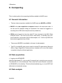
9. Beamline
6. Computing
This is a short guide to the computing facilities available to MuSR users.
6.1 General Information
•
The two cluster computers available for MuSR users are MUSR and ISISA.
• MUSR is the data acquisition computer located in the instrument cabin. It
can be used for analysis during an experiment, but cannot be logged in to
remotely (due to ISIS-wide computer security measures).
• ISISA can be logged into from the cabin PC, from terminals in the DAC (Data
Analysis Centre – the room by the users’ coffee area), or remotely from your
home institution, and can be used for data analysis, etc. It is the only ISIS node
that can be logged into from off-site.
•
The account MUSR01 is available to all users for data analysis.
•
The PC in the MuSR cabin can be used for normal PC applications (Microsoft
Office, Origin, SigmaPlot, Fortran) and as a terminal on to one of the cluster
computers using the eXceed application.
6.2 Data acquisition
• Logging onto NDXMUSR
Using the right hand PC ( the one with 2 screens) log in using the musr account.
The password is on the whiteboard. Then select the remote terminal connection
to NDXMUSR on the desktop. This should automatically log you in and SECI will
either start or already be running.
6.3 Data analysis
22/02/05
9. Beamline
6.3.1 Logging on
•
Logging in through an Xterminal. These terminals are available for users
in the Data Analysis Centre (DAC). Click on the ‘CREATE’ option at the top
of the terminal manager window, and select ‘DECterm’ followed by the
machine you wish to connect to. Then log in as normal using either the
MUSR01 account or your own account.
•
Logging in through a PC. The PC in the MuSR cabin (and other public
access PCs) can be used as terminals to log on to ISISA using the eXeed
application. On the MuSR PC, click on one of the terminal icons on the
desktop. If you choose one of the MUSR01 icons, you will just be asked for
the current password; otherwise, enter a username and password. A terminal
window will appear after a few seconds. In order to allow graphics displays
from UDA and other software to appear on the PC screen, it is necessary to
type
SET DISPLAY/CREATE/NODE=<node>/TRANSPORT=TCPIP,
where <node> is the IP number of the PC you are using (the node
name and IP number of the MuSR PC. This can be found by typing
ipconfig in a DOS command prompt).
6.3.2. Using the MUSR01 account for data analysis
1. Log on to S
I ISA or MUSR with the username MUSR01. The password is
changed periodically - contact an instrument scientist to obtain the current one.
2. Once access has been obtained, a list of users known to the account is
displayed. Select the most appropriate, or alternatively use USERX, and type
the name at the prompt. The cursor should change to reflect the current user.
For example, USERX would proceed as follows:
Users
SCRATCH
known:
RAL
RUNI
STUTTGART
SOTON
BS
LPOOL
STANDREWS
22/02/05
CSIC
PARMA
CNRS
BIRMINGHAM SUSSEX
UPPSALA
ILL
OXFORD
USERX
PARIS
SHEFFIELD
LEICESTER
BRAUNSCHWEIG
LYON
9. Beamline
MUSR01>
USERX
***********************************************************
YOU
FILES
ARE
IN
NOW
THIS
WORKING
AREA
USE:
ON
WILL
BE
SETUP
THE
SCRATCH
DELETED
AFTER
to
DISK
7
access
DAYS
UDA
***********************************************************
USERX>
3. Now type SETUP. A list of the analysis software currently available will be
displayed. Any of these may be used by typing the program name. For
example, to run UDA, USERX would proceed as follows:
USERX>
SETUP
Commands
available:
TLOGGER
-
HISTO
-
plot
look
temperature
at
the
raw
logs
histograms
CONVERT_ASCII - turn the binary run data into ASCII format
HEADERS - make a list of MuSR data file header information
ASYM
UDA
-
analyse
-
standard
RESTMUSR
PRINT_MAN
-
print
-
SUPERPLOTC
-
access
muon
restore
SUPERPLOT
If
levelcrossing
to
the
datafile(s)
MuSR
manual
general
for
RUMDA
data
on
analysis
from
LSR5
(MuSR
plotting
plotting
is
data
required
archive
Cabin)
program
in
type
colour
RUMDA
If access to MESA or TDSA is required type MESA_SETUP
USERX>
UDA
4. If access to RUMDA and GENIE is required type RUMDA. Again, a list of the
available commands will be displayed which give access to the RUMDA
programs. TDSA, an alternative analysis program, and MESA, a maximum
entropy analysis program for transverse field data, are available MESA_SETUP.
22/02/05
9. Beamline
6.3.3 Using your own account for data analysis
1. Login to ISISA or MUSR with your own user name and password
2. Type @musr$disk:[mumgr.musr_users]musr_setup to gain access to the
data analysis software.
3. You may want to edit your LOGIN.COM file (found in your top-level
directory) to add the line (preferably at the end of the file):
$ setup :== “@musr$disk:[mumgr.musr_users]musr_setup”
4. Typing SETUP when you next login will work as described above for
the MUSR01 account.
NB.
two
If you use both MuSR and EMU instruments, you may wish to add
lines
to
your
LOGIN.COM
file,
one
for
MUSR_SETUP
and
one
for
EMU_SETUP, as the SETUP files for the two instruments are different.
The EMU_SETUP command can be found in the EMU User Guide.
6.4 Utility programs
6.4.1 CONVERT_ASCII: converting data files to ASCII format
The binary files written by MCS can be converted into ASCII files in one of three
formats: firstly, in the same format as read by UDA’s ‘USRFILE’ option; secondly,
as a column of raw counts for each histogram (this is ideal for loading into PC
spreadsheet applications); thirdly, as asymmetry data (this format can be directly
imported into PC analysis programs such as Origin). The conversion program is
run from account MUSR01 using the command CONVERT_ASCII. The program
prompts for first and last files to be converted and the format of the output ASCII
data. Depending on the output ASCII file format required, additional information
may be requested.
When using format options two or three it is very important that correct values are
entered for both the t0 and α. Check also that the grouping used in option three
corresponds to the current detector arrangement.
22/02/05
9. Beamline
6.4.2 TLOGGER: plotting TLOG files
A plot of the temperature log for a data run may be produced using the command
TLOGGER. The program will request the beamline (select option '2' for MuSR), a run
number and the type of graphics device you are using to view the plot (enter /xw
when using DECwindows). The file number need not have preceding zeros. The
TLOG file with highest version number is plotted for the given run; files with lower
version numbers are displayed by typing the complete file ending: e.g.
00123.TLOG;1 will plot R00123.TLOG;1. The hard copy option produces a
postscript file PGPLOT.PS, and this may then be sent to the MuSR laser printer
using the command PRINT/QUEUE=POST$LSR5 PGPLOT.PS.*.
6.4.3 ISISNEWS: the status of ISIS
Typing ISISNEWS CURRENT at the DEC prompt gives news on the status of ISIS.
Information may also be obtained from looking at the messages in Bulletin, type
BULLETIN at the prompt.
6.4.4 Archiving data on to a PC floppy disk
Data may be archived on to an IBM PC format floppy disk as follows:
• Convert all data files to ASCII format using CONVERT_ASCII.
• On a PC launch the FTP application by double clicking the left mouse button
on the 'WS_ftp32' icon on the left of the desktop.
• The program automatically comes up with a window requesting details of the
connection to be made. The ‘host name’ should be set to isisa.rl.ac.uk.
•
•
•
•
Enter a user name (eg. MUSR01) and password and click on OK.
When the connection is made and WS_ftp32 has read in the remote directory,
set the appropriate PC directory using the ChgDir box on the left hand side of
the WS_ftp32 window (set this to a: for transfer to a floppy), and the
mainframe directory on the right hand side (for the MUSR01 account, files will
be in scratch$disk:[musr01.users.userx] where you should replace userx
with your own area name.
For ASCII data, ensure that the ASCII button, below the windows showing
files, is checked.
Highlight the files you wish to transfer and click the appropriate arrow between
the two file windows to copy the files.
Further information can be found in the on-line help within the program.
22/02/05
9. Beamline
6.5 The MuSR PC
The PC in the MuSR cabin is available for use as a terminal or to use one of the
software packages installed (the PC has Microsoft Office and Origin, as well as
normal applications). If it becomes necessary to reboot the PC, the login name
and password are on the board in the cabin. To start applications, either click on
the appropriate icon on the bar on the right hand side of the screen, or use the
‘START’ menu from the bottom bar. Please ask your local contact for further
information if you are unfamiliar with the Windows XP system.
6.6. Printers
The following printers are available for users:
Black and white laser printers:
LSR0 (R3 Computer Support Office),
LSR1 (R3 2nd floor),
LSR2 (R55, DAC)
LSR3 (MARI cabin)
LSR4 (CRISP cabin)
LSR5 (MuSR cabin)
LSR7 (PRISMA cabin)
LSR8 (SXD cabin)
LSR10 (outside EMU cabin)
LSR11 (HET cabin).
Colour printers:
R3_COL00 (R3 Computer Support Office)
R3_COL01 (R3 2nd Floor),
POST$INK0 - (Deskjet 1200 in MARI),
POST$INK2 (Deskjet 1200 in DAC),
POST$INK4 (Deskjet 1200 in CRISP).
To print PostScript files on the MuSR cabin printer:
print/que=post$lsr5 [file.ps]
22/02/05
9. Beamline
and to print text files:
print/que=ansi$lsr5 [file.txt]
22/02/05
9. Beamline
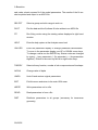
7. Data acquisition: SECI
The sample environment and data collection on MuSR are controlled by a
computer program "SECI" running on the computer NDXMUSR.
Starting a Run
Type
begin
Ending a Run and saving the data
Type
end
Ending a run without saving
Type
abort
Pausing a run
Type
pause
Then to continue the run
Type
resume
Setting a temperature
Type
Setting a field
Type
settemp <value>
setmag <value>
Selecting T20 power supply and setting 20Gauss
Type
TF20
Selecting Danfysik power supply
Type
lf0
Selecting auto-zerofield
22/02/05
9. Beamline
Type
f0
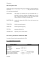
Automatic running of MuSR
Scripts are created on the mkscript3 panel and should be saved
on the u: drive. To load a script
Type
load “u:\<nameof script>.gcl”
To run a script
Type
Runscript
To keep the current run going type keep in the custom column
To end a script
Type
<crtl> C
Should mkscript3 crash then the easily way to restart
mkscript3 is to restart SECI.
Under Start (bottom left) press killseci.cmd
Wait a minute or so
Then under Start press startstation.cmd
If this is not possible or desirable then the mkscript3.exe
program
can
be
found
in
directory
“c:\labview
modules\mkscript3”. However, SECI will not have control of
the window.
Setting the label
Type setlabel /qualifier
/s for sample
/c for comment
/u for user
/rb for rb number
/t for temperature
/f for field
/g for geometry
/o for orientation
You will be prompted for information
22/02/05
9. Beamline
Changing configurations:
- Select Configurations from the ISIS SECI window
- Select Open Configuration
- Select Correct configuration (please do not save
configurations)
- SECI should start the correct vi’s which are currently not
running and close any that are not needed
- Type getblocks in the Opengenie window
Blue Cryostat
For operation below 5K
Type
For operation above 5K
Type
blue_lt
blue_ht
The temperature parameter files:
For all configurations the tpar files are in “C:\labview
modules\mkscript3”
directory
and
are
called
“muon_temperature.tpar”
Displaying all control blocks
Type
22/02/05
cshow/all
9. Beamline
8. Data analysis: UDA
8.1 Introduction
UDA is the simplified µSR data analysis program. There are three menus in
UDA, the Main Data menu, the UDA data Grouping menu and the UDA data
Analysis menu.
On start-up the program will always enter the Main menu. At this menu you can
read and write data files, plot spectra and make changes to the data loaded.
In the data Grouping menu you can select how to map your raw histograms into
the "groups" that are used when plotting or analysing. Two different grouping
schemes can be used, the Simple (straight, TF) grouping, or the F-B (LF,ZF)
grouping. Deadtime correction of data is available using the same correction
method as the RUMDA analysis program.
In the Analysis menu you can select a model function and make a least-squares
fitting of the model parameters. The fitting result can also be plotted from this
menu.
8.2 Running UDA
To access UDA from account MUSR01 type SETUP followed by UDA as
described in section 6.3. This will run the most recent version of UDA. The
display will be redrawn as a dashboard and the cursor will automatically select
the option MCSFILE in the Main menu. To select any other item from the menu
use the cursor (arrow) keys or simply type the first letter of that item (e.g. ‘P’ for
PLOT).
8.3 The Main Data Menu
22/02/05
9. Beamline
The Main Data menu allows you to read, write and modify experimental data. The
options available from this menu are listed below. Plotting of error bars on data
points can be turned off/on using the SETUP option.
MCSFILE
Read a MCS run file in the format used by the data acquisition
software
USRFILE
Read a uSR file from the disk
NEXUS
Read a NeXus File (the new and only data format on MusR)
WRITE
Write (grouped) data to a uSR file
INSPECT
Inspect run and all histograms
GROUP
Enter the Grouping Menu
CHANGE
Change run file parameters
PLOT
Plot one or more groups on the terminal screen
ANALYSE
Enter the analysis menu
SETUP
Set program configuration parameters
HELP
Enter the VAX/VMS help facility to read the UDA help library.
QUIT
Exit UDA and return to VMS prompt
8.4 The Grouping Menu
The grouping menu is accessed through the option "Group" from the Main menu,
and defines the grouping and correction of raw histogram data. There are
currently two ways of grouping the histograms:
a) the Simple grouping, where histograms are simply added together.
b) the Forward-Backward (F-B) grouping, where the 'asymmetry ratio'
(F-αB)/(F+αB) is calculated.
22/02/05
9. Beamline
Deadtime correction of data is turned on/off using the DeadT option. To
compensate for deadtime, UDA uses the same file of deadtime values as the
RUMDA analysis program, generated at the start of each cycle from a long silver
run. Please ask your local contact if you are analysing data from a previous cycle
and so require UDA to use deadtime values from that cycle rather than the current
deadtime file. The effects of deadtime correction are shown in figure 16 of
section 9.3.
The options available for grouping and correcting data are shown below.
CHANGE
Change histogram grouping
READ
Read grouping table from disk
WRITE
Write grouping table to disk
DEADT
Switch deadtime correction on/off
ALPHA
Select (F-B) scaling factor
GUESS
Estimate alpha for a T20 run
BUNCH
Setting the bunching to ‘n’ adds ‘n’ bins together.
HELP
Display help text. (Don't panic)
EXIT
Return to UDA Data (main) menu
8.5. The Analysis Menu
The Analysis menu is entered by selecting the option ”Analyse” in the UDA Main
menu. Using the options outlined below it is possible to select a model function
22/02/05
9. Beamline
and make a least squares fit of the model parameters. The results of the fit can
also be plotted and output to an ASCII file.
SELECT
Select a group and a bin range to work on.
PLOT
Plot the data and the fit; allows fit to be written to an ASCII file
FIT
Run fitting routine using the starting values displayed in right hand
window
HELP
Enter the help system at the Analysis menu level
VALUES
Enter the parameter display to change parameter values/status.
To move in the parameter display use UP or DOWN cursor keys.
To change a value use the ENTER key. Status codes are changed
by typing ~ (vary parameter), ! (fix parameter), = (tie parameters
together). Return to the menu by the left or right cursor keys.
THEORY
Select a theory function, number of sub-components and lineshape
ALPHA
Change value of alpha
UNDO
Undo fit and restore original parameters
EXIT
Exit this menu and return to the main UDA menu
WRITE
Write parameters out to a file
READ
Read parameters in from a file
DIST
Distribute parameters to all groups (necessary for transverse
geometry)
22/02/05
9. Beamline
8.6 Computer files
These files must be copied into the area you are working in. If the area has been
selected by SETUP (as described in section 6.3) they will have been copied
to the new area automatically.
SETUP.UDA
UDA reads some variables from the file SETUP.UDA. In
particular the directory address of the data is set up in this
way. Of particular interest are the FORTRAN format strings
used to convert a run number to a full file name.
BASETIME.UDA
contains the value which UDA will use for time-zero (see
section 8.8).
TRANS.UDA
default transversal grouping
LONG.UDA
default longitudinal grouping
PDF.UDA
parameter definition file
UDAHELP.HLP
help library source, UDA matters
8.7 Theory functions defined in UDA
A number of theory functions are predefined in UDA:
8.7.1 Longitudinal and zero field
Function Name
1. Lorentzian
2. Gaussian
3.
LX(exp)
Stretched
Exponential
4. Keren LF (extended Abragam)
5. Kubo-Toyabe (Gaussian)
6. Kubo-Toyabe (Lorentzian)
22/02/05
Definition
a o exp( − λt )
a o exp( − ( λt ) 2 )
a o exp( − (λt ) β )
a 0 exp ( − Γ (t)t) ; see note 1 below
a o ( 1 3 + 2 3 (1 − (λt ) 2 ) exp( − ( λt) 2 2 ))
a o ( 1 3 + 2 3 (1 − λt ) exp( − λt ))
9. Beamline
8. Dynamic Kubo-Toyabe
Note
see note 2 below
1:
2∆
{[ωs2 +ν 2 ]νt + [ωs2 − ν2 ] × [1 − exp(−νt)cos(ωs t)] − 2νωs exp(−νt)sin(ωs t)}
2
2 2
(ωs + ν )
2
Γ (t)t =
where UDA’s sigma is equivalent to ∆, UDA’s tau is equivalent to 1/ν and
ωs=γµB0.
Note 2: Function 8, the dynamic Kubo-Toyabe, uses numerical integration to
produce the fitting function and so requires more time than the other functions.
Only fit up to channel 1000 when using this option.
8.7.2 Transverse field
Function Name
Definition
a o cos(ωt + φ ) exp( − λt )
11. Lorentzian with freq
a o cos(ωt + φ ) exp( − (λt ) 2 )
12. Gaussian with freq
β
13. LX(exp) - Stretched a o cos(ωt + φ ) exp( − ( λt ) )
Exponential with freq
a o cos(ωt + φ ) exp( − ( λτ c ) 2 (exp( − t τ c ) − 1 + t τ c ))
14. Abragam with freq
8.8 Time-zero
Time-zero is usually taken to be the arrival time of the centre of the muon pulse.
On MuSR, which receives the second of the two muon pulses produced by the
proton beam, this is found to be 0.645 µs after the timing start signal produced by
the Cerenkov counter near the muon production target. This corresponds to
slightly after the start of bin 40 in the detector histograms (for a bin size of 16 ns).
UDA uses this value to set its time-zero position (it is written in the file
basetime.uda). However, useful data is not produced until after the complete
arrival of the muon pulse, so that bins 46 and above can be used for function
fitting, etc.
22/02/05
9. Beamline
9. Other components of the muon
beamlines
9.1 Beamline power supplies
Located at intervals along the muon beamline between the production target and
the spectrometer are dipole and quadrupole magnets which respectively act to
steer and focus the muon beam (see figure 1 at the foot of the Contents pages).
Most of the beamline magnets are located before the kicker, and therefore any
faults will affect all three muon beamlines; however there are also two
quadrupoles specifically for MuSR located after the kicker. The power supplies
for all the beamline magnets are located on the raised platform on the far East
side of the experimental hall (the steps up to this are opposite the steps taking
you over the proton beam to the other side of the hall).
On the left at the top of the steps on the platform, and working towards the far wall,
are the following units:
1
2
3
6
9
4
7
10
5
8
11
15
12
13
14
16
17
20
23
18
21
24
19
25
22
26
Figure 16. Beamline power supply layout
1
2
3
4
5
6
7
8
9
Reset buttons for beamline magnet klixons, flow and earth leakage trips
Q1 supply
Separator B-field supply
Q2 supply
Q3/5 supply
Q4 supply
Q6 supply
Q7 supply
Q8 supply
22/02/05
9. Beamline
10
11
12
13
14
15
16
17
18
19
20
21
22
23
24
25
26
Q9 supply
B1/2 supply
DEVA Helmholtz supply
DEVA septum supply
EMU septum supply
Reset buttons for quads/coils on individual beamlines
Panels showing on/off status of klixons, etc, for quad/coil supplies
Q10A supply (DEVA)
Q11A supply (DEVA)
Q12A supply (DEVA)
Q10B supply (MuSR)
Q11B supply (MuSR)
switchyard magnet supply
Q10C supply (EMU)
Q11C supply (EMU)
Q12C supply (EMU)
switchyard magnet supply
The normal working currents for these supplies are shown by them, but call your
local contact if you think there is a fault.
9.2 The separator
The separator is located in the muon beamline before the kicker and acts to
remove contaminant particles (primarily positrons) from the muon beam. It
consists of mutually perpendicular E and B fields which act as a velocity selector.
The settings of the two fields are correlated so that muons of a particular velocity
are transmitted: with the E field at 100 kV, the B field supply must be run at 43 A
(and with E at 90 kV, the B field requires 39 A, etc). The power supply for the B
field is located with the other beamline power supplies (see section 9.1); the E
field is controlled from a unit located below the mezzanine floor behind the EMU
area. The required voltage for the separator E field can only be achieved by
‘conditioning’; that is slowly increasing the voltage until the field breaks down and
leaving it at this setting for a period before increasing it further. This process is
done at the start of each cycle, but is often required during the middle of a cycle if
the separator voltage becomes unstable.
22/02/05
9. Beamline
9.2.1 Spin rotation by the separator
When the muon beam is deflected by a magnetic field the spin and momentum
vectors remain collinear. However, the same is not true if the beam is passed
through an electric field, when the muon spin is rotated with respect to its
momentum vector. The effect of the electric field in the separator is to rotate the
muon polarisation upwards slightly by about 6o so that there is a component
transverse to the momentum direction. This rotation is best observed by
examining individual detectors for data taken in small longitudinal fields (up to
~400 G). Under these circumstances there is a precession of the muon spin in
the field and an oscillating signal can usually be seen. Shown below is the signal
from detector 1 for a silver sample in an applied longitudinal field of 50 G. The
oscillations shown have an asymmetry of 2.2%.
10
asymmetry
5
0
-5
-10
0
2
4
6
8
time (µs)
Figure 17. Spin rotation by the separator seen in a single detector
By grouping the detectors, however, the effect is removed. The graph below
shows the data from this run arranged into a forward-backward grouping. This
plot also shows the effects of deadtime: the grouped data is displayed with
(crosses) and without (line) deadtime corrections.
22/02/05
9. Beamline
26
asymmetry
25
24
23
22
21
20
0
2
4
6
8
time (µs)
Figure 18. Grouped data with and without dead time correction
9.3 The kicker
The kicker is responsible for supplying muons to the DEVA and EMU areas.
Muons are generated at the production target with the same time structure as the
main proton beam, i.e. two 80 ns wide pulses separated by 300 ns (50 times per
second). The first of these pulses is split in two in the kicker by a central
electrode at high voltage. This kicks half the pulse to the left and half to the right,
feeding the two side beamlines. In the time between the two muon pulses the
voltage on the electrode is reduced to zero, and the second pulse travels
undeflected to MuSR. The kicker power supply is located under the mezzanine
floor behind the EMU area and consists of a high voltage supply together with
timing electronics to ensure that the kick occurs at the correct point with respect
to the muon pulses. The timing signal is taken from a lead glass Cerenkov
counter located near the muon production target and fed to a delay unit.
Instructions on how to reset the kicker are given in section 10.5, but this should
only be done by an instrument scientist.
9.4 The photomultiplier tubes
The photomultiplier tubes on the spectrometer are powered from one of the
LeCroy crates in the back of the EMU cabin. (The crates are labelled MuSR and
EMU - make sure you switch the correct one on or off if you have to). Slots 2 and
3 of the MuSR crate are used to power the MuSR PMTs, with 16 outputs from
22/02/05
9. Beamline
each slot (addressed 0-15, not 1-16). Once the LeCroy crate is powered up it
can be controlled from the terminal in the back of the MuSR cabin. It should only
be necessary to modify the PMT voltages in two circumstances:
•
when rotating the instrument all tubes should be turned OFF (don’t forget to
turn them back on again afterwards!)
•
if a scintillator develops a light leak, please turn off the volts to its PMT.
The most commonly used commands for controlling the PMTs from the terminal
are shown in the table below.
Command
Action
ON,OFF
switch the voltage on all tubes on or off
RE(2-3,0-15)
displays the voltage on all MuSR PMT
tubes
RE(slot, channel)
displays the voltage on one tube
WR(slot, channel)0
sets the voltage on a single tube to zero
WR(slot, channel)v
sets the voltage on a single tube to v
Ctrl C
stops screen scrolling
22/02/05
10. Troubleshooting
10. Troubleshooting
10.1 No muons
• Check the machine is running at a reasonable rate. In the MuSR cabin there is
a proton per pulse (PPP) monitor displaying the pulse intensity in µA. If this
reads 00 there are no protons, and if it is flashing any number then ISIS is not
running at 50 Hz and therefore the count rate will be lower than usual.
• If ISIS is not running, check the facility status by typing ISISNEWS current in a
decterm (not mcs control window) or http://www.isis.rl.ac.uk/status/index.htm
• Check the beam blocker is open: the gate must be closed and locked to allow
this. The blue interlock light will be lit if this has been done correctly.
• Check that the high voltage to the photomultiplier tubes is on (this is particularly
likely to be the problem immediately after the instrument has been rotated).
The red lights on the photomultiplier tube bases should be on. If not, type ON on
the terminal controlling the high voltage power supply in the back of the MuSR
cabin (see section 9.4 for further details of the photomultiplier tube high voltage
commands).
• Check the ‘BEAM OFF’ button on the fence in the zone is not pressed. If it is,
release it, then restart the bending magnet power supply, B1/2, above the
cryostat store using only the ‘START’ button (see section 9.1).
• Check that all the magnets are working by checking their power supplies (see
section 9.1 - the current they should be set at is written on each). If necessary,
reset or restart using the value given.
• Check that the kicker is working. Instructions for resetting it if it has tripped are
at the end of this chapter, but please consult your local contact before doing
this.
• Check that the separator is at its correct voltage - typically 90 kV.
22/02/05
10. Troubleshooting
10.2 Computer Problems: Restarting SECI
Goto the Start Menu and select killSECI. After SECI has stopped goto the start
menu again and select startstation. If this does not resolve the problem then
rebooting NDXMUSR might be necessary this can be done by type “ctrl –alt –
end” together and then select shutdown. Please select restart or NDXMUSR will
not restart!
10.3 Resetting the kicker
If the spectra from the individual detectors displayed on the MuSR data
acquisition screen shows the effects of a double pulse the electrostatic kicker has
failed and all the muons are passing undeflected through to MuSR. Before
resetting the kicker check with the EMU and DEVA users that they have lost all
beam. In most cases EMU and DEVA users will notice a kicker failure before
MuSR users. The instructions for resetting the kicker are given below and are
also attached to the kicker power supply unit.
•
Turn key switch A through 90° to OFF position
•
Turn helipot B fully anticlockwise to 0.0 volts
•
Wait a few seconds
•
Turn key switch A through 90° back to ON position
•
Observe LED display on front panel. Only the +120I(A) and +120I(B) and the
(large) "DELAYED POWER ON" should be unlit at this stage
•
After 120s the +120I(A) and +120I(B) LEDs will light
•
After a further 180s the "DELAYED POWER ON" will light and the high
voltage power supply will be powered up
22/02/05
10. Troubleshooting
•
Dedicated trigger should light
•
While pressing the "READ SET VOLTS" push button turn helipot B slowly
clockwise to obtain a set volts readout of 32.5kV. The current read-out will be
∼2.02mA when the push button is released
22/02/05
10. Troubleshooting
READ SET VOLTS
PUSH BUTTON
FAN UNIT
SET VOLTS READOUT
kV
MAINS ON SWITCH
HIGH VOLTAGE
POWER SUPPLY
mA
SET CURRENT LIMIT
SET VOLTAGE B
SET CURRENT
HELIPOT
o
o o o o
o o o o
o
o
DG53
o
120 I(A)
120 I(B)
o o
o
o
o
o
o
o
o
o
o
o
o
o
o
o
o
o
o
o
o
o
o
o
TRIGGER
TIMING UNIT
o o
INTERLOCK
UNIT
elapsed time delay
relay
o o
INTERLOCK
LED
DEDICATED
TRIGGER
LEDS
DELAYED
POWER
ON
ON/OFF KEY A
THYRATRON POWER
SUPPLY
VENT
FILTER
FAN
FAN
FILTER
Figure 19. Reference diagram for resetting the kicker
22/02/05
11. Contact Points
11. Contact Points and further information
11.1 Laboratory contact points
Rutherford
Chilton,
Didcot,
Oxfordshire,
OX11 0QX.
Appleton
( (01235) 821900
( +44 1235 821900
Laboratory,
(national)
(international)
Main control room (MCR)................(6789
EMU cabin (R55) .............................(6831
MuSR cabin (R55) ...........................(6135
DEVA cabin (R55)...........................(6851
Experimental Areas .........................(6338
ARGUS/RIKEN…………………….(6766
Health Physics/ Sample checking ..(6696
Computer support ............................(1763 (7770858090 from outside the lab)
University Liaison Office..................(5592
Cosener's House .............................(3007 or (01235) 523198
Local taxi’s.......................................(5592 (during the night ring the MCR)
Airport transportation (24hrs notice required) (5592
Gas bottles (He, N2 etc) ...................(6166
11.2 Contacting an instrument scientist
Stephen Cottrell
Adrian Hillier
Philip King
James Lord
Francis Pratt
22/02/05
(5352 or 1665
(6001 or 1476
(6117 or 1716
(5674 or 1101
(5135
(Email: [email protected])
(Email: [email protected])
(Email: [email protected])
(Email: [email protected])
(Email: [email protected])
11. Contact Points
From outside the laboratory certain extensions may be direct dialled, the
number being formed in the following manner:
(01235) 44xxxx, where 'xxxx' is the required extension.
No prefix is needed to dial offsite.
11.3 Further information on the ISIS muon beamlines
For further information on the ISIS muon beamlines, see
Commissioning of the Rutherford Appleton Laboratory pulsed muon
facility GH Eaton et al. Nucl. Inst. Meth. A269, 483-491, 1988.
The ISIS pulsed muon facility: past, present and future A Carne et al.
Hyperfine Interactions 65, 1175-1182, 1990.
UPPSET: a pulsed electrostatic kicker to improve the µSR frequency
response in the ISIS pulsed muon beam AI Borden et al. Nucl. Inst. Meth.
A292, 21-29, 1990.
The ISIS pulsed muon facility GH Eaton Z. Phys. C 56, S232-239, 1992.
The muon beamline at ISIS GH Eaton et al. RAL Report RAL-94-077.
The development of the pulsed muon facility at ISIS GH Eaton et al.
Hyperfine Interactions 87, 1099-1104, 1994.
Fast E-field switching of a pulsed surface muon beam: the
commissioning of the European muon facility at ISIS GH Eaton et al. Nucl.
Inst. Meth A342, 319-331, 1994.
The ISIS muon group Web pages also contain additional information on the muon
facility, as well as the current instrument schedules, etc.; the address is
http://www.isis.rl.ac.uk/muons
22/02/05
11. Contact Points
The main ISIS web pages contain details of all ISIS facility activities, together with
information on applying for beamtime, electronic versions of proposal forms and
A3 report forms, latest beam information, etc. They can be found at
http://www.isis.rl.ac.uk.
11.4 Local information
22/02/05
11. Contact Points
Transport
National Rail Enquiries
It is usually possible to arrange a taxi to either
Didcot Parkway or Oxford stations.
The Oxford Bus Company
Oxford city local buses and coaches to London
(X90), Heathrow (X70) and Gatwick (X80).
0345 48 49 50 or
http://www.railtrack.co.uk/travel/
01865 785400
http://www.oxfordbus.co.uk/
index.html
Stagecoach Bus Company (formerly Thames
Transit)
01865 727000
Oxford city and rural bus services including routes
to/from Harwell bus station near main gate.
BAA Flight Information
Arrival information for many UK airports including
Heathrow and Gatwick.
http://www.heathrow.co.uk/
baainfo/baainfht.html
General Information
Oxford Tourist Information Centre
01865 726871
Oxford Guide on the Web
http://www.comlab.ox.ac.uk/
archive/ox/
Eating and Drinking
Didcot Tandoori, 222 Broadway, Didcot
Chhokar Tandoori, 226a Broadway, Didcot
01235 812206
01235 813573
Cherry Tree Inn, Steventon
Fleur de Lis, East Hagbourne
The George and Dragon, Sutton Courtenay
The Great Western Junction Hotel, Didcot
The Hare Inn, West Hendred
The Harrow, West Ilsley
The Plough, Sutton Courtenay
Red Lion, Drayton
Rose and Crown, Chilton
The Swan Inn, Sutton Courtenay
The Wheatsheaf Inn, East Hendred
01235 831222
01235 813247
01235 848252
01235 511091
01235 833249
01635 281260
01235 848801
01235 531381
01235 834249
01235 847446
01235 833229
22/02/05