1
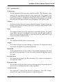
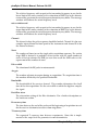
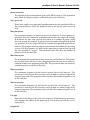
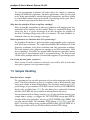
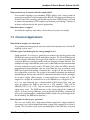
picoSpin-45 User’s Manual
Release 0.8.0-32
picoSpin, LLC
July 07, 2011
CONTENTS
1
Welcome
1.1 Getting Started . . . . . . . . . . . . . . . . . . . . . . . . . . . . . . . . . . .
1.2 Software Updates . . . . . . . . . . . . . . . . . . . . . . . . . . . . . . . . . .
1
1
2
2
NMR Spectroscopy
2.1 References . . . . . . . . . . . . . . . . . . . . . . . . . . . . . . . . . . . . . .
3
3
3
Quick Start
3.1 What’s in the Box . . . . . . .
3.2 Ethernet Connection . . . . .
3.3 Magnet Temperature Control
3.4 Injecting a Sample . . . . . .
3.5 Finding the Signal . . . . . .
3.6 Auto Shimming . . . . . . . .
3.7 Your First Spectrum . . . . .
.
.
.
.
.
.
.
.
.
.
.
.
.
.
.
.
.
.
.
.
.
.
.
.
.
.
.
.
.
.
.
.
.
.
.
.
.
.
.
.
.
.
.
.
.
.
.
.
.
.
.
.
.
.
.
.
.
.
.
.
.
.
.
.
.
.
.
.
.
.
.
.
.
.
.
.
.
.
.
.
.
.
.
.
.
.
.
.
.
.
.
.
.
.
.
.
.
.
.
.
.
.
.
.
.
.
.
.
.
.
.
.
.
.
.
.
.
.
.
.
.
.
.
.
.
.
.
.
.
.
.
.
.
.
.
.
.
.
.
.
.
.
.
.
.
.
.
.
.
.
.
.
.
.
.
.
.
.
.
.
.
.
.
.
.
.
.
.
.
.
.
.
.
.
.
.
.
.
.
.
.
.
.
.
.
.
.
.
.
5
5
7
8
9
10
12
15
System Operation
4.1 Web Browser Interface .
4.2 Sample Handling . . . .
4.3 Shimming . . . . . . . .
4.4 Changing the Cartridge
.
.
.
.
.
.
.
.
.
.
.
.
.
.
.
.
.
.
.
.
.
.
.
.
.
.
.
.
.
.
.
.
.
.
.
.
.
.
.
.
.
.
.
.
.
.
.
.
.
.
.
.
.
.
.
.
.
.
.
.
.
.
.
.
.
.
.
.
.
.
.
.
.
.
.
.
.
.
.
.
.
.
.
.
.
.
.
.
.
.
.
.
.
.
.
.
.
.
.
.
.
.
.
.
.
.
.
.
19
19
19
19
19
5
Experiment Scripts
5.1 onePulse . . . . . . . . . . . . . . . . . . . . . . . . . . . . . . . . . . . . . . .
5.2 autoShim . . . . . . . . . . . . . . . . . . . . . . . . . . . . . . . . . . . . . .
5.3 search . . . . . . . . . . . . . . . . . . . . . . . . . . . . . . . . . . . . . . . .
21
22
25
28
6
Hardware Description
6.1 Magnet . . . . . . . . . . . . . . . . .
6.2 Capillary Cartridge . . . . . . . . . .
6.3 RF and Data Acquisition Electronics
6.4 Shim System . . . . . . . . . . . . .
6.5 Specifications . . . . . . . . . . . . .
33
33
33
34
34
34
4
.
.
.
.
.
.
.
.
.
.
.
.
.
.
.
.
.
.
.
.
.
.
.
.
.
.
.
.
.
.
.
.
.
.
.
.
.
.
.
.
.
.
.
.
.
.
.
.
.
.
.
.
.
.
.
.
.
.
.
.
.
.
.
.
.
.
.
.
.
.
.
.
.
.
.
.
.
.
.
.
.
.
.
.
.
.
.
.
.
.
.
.
.
.
.
.
.
.
.
.
.
.
.
.
.
.
.
.
.
.
.
.
.
.
.
.
.
.
.
.
.
.
.
.
.
.
.
i
7
ii
Frequently Asked Questions
7.1 General Questions . . .
7.2 Sample Handling . . . .
7.3 Chemical Applications .
7.4 Installation . . . . . . .
7.5 Data Analysis . . . . . .
.
.
.
.
.
.
.
.
.
.
.
.
.
.
.
.
.
.
.
.
.
.
.
.
.
.
.
.
.
.
.
.
.
.
.
.
.
.
.
.
.
.
.
.
.
.
.
.
.
.
.
.
.
.
.
.
.
.
.
.
.
.
.
.
.
.
.
.
.
.
.
.
.
.
.
.
.
.
.
.
.
.
.
.
.
.
.
.
.
.
.
.
.
.
.
.
.
.
.
.
.
.
.
.
.
.
.
.
.
.
.
.
.
.
.
.
.
.
.
.
.
.
.
.
.
.
.
.
.
.
.
.
.
.
.
.
.
.
.
.
.
.
.
.
.
.
.
.
.
.
35
35
36
37
38
38
CHAPTER
ONE
WELCOME
Welcome to the User’s Manual for the picoSpin-45 NMR spectrometer. This document is
available on the support page of the picoSpin web site in both HTML and pdf formats.
There is also an HTML version installed on your picoSpin-45 spectrometer.
Make sure the version number of the documentation you are viewing is the same as the
installed software version on your picoSpin-45 spectrometer.
Version 0.8 is the first released version of the picoSpin software. It includes an embedded
web server that allows users to control the spectrometer from a web browser anywhere on
their local network. The server also provides live preview of time and frequency domain
data, selection and control of experiment scripts, data storage and download, interfaces to
the shim and temperature control hardware, and a software update function. Experiment
scripts included in version 0.8 support spectroscopy with complete control of experimental parameters, automatic shimming and signal search. These scripts support most of the
anticipated applications of the picoSpin-45.
Version 0.9 will provide enhancements to the browser interface and additional experiment scripts including T1 inversion-recovery and nutation curves. With the release of
version 1.0 we will provide documentation and new functionality that will allow users to
write their own experiment scripts and pulse sequences.
1.1 Getting Started
If you are new to the picoSpin-45 and want to get started right away, go to the Quick Start.
You may also want to browse the picoSpin Frequently Asked Questions and view the full
Contents. For technical support, contact picoSpin using this form. If you are unfamiliar
with the basics of NMR or you need a refresher, go to NMR Spectroscopy.
1
picoSpin-45 User’s Manual, Release 0.8.0-32
1.2 Software Updates
The picoSpin software system is updated regularly. picoSpin customers may register here
to recieve e-mail notification of software updates as soon as they are available. A link for
downloading the update files will be provided. Instructions for installing updates can be
found on the spectrometer’s Settings page.
2
Chapter 1. Welcome
CHAPTER
TWO
NMR SPECTROSCOPY
Readers of the picoSpin-45 User’s Manual should be familar with the basics of pulsed
NMR spectroscopy of liquids. An introduction to this subject can be found in any collegelevel organic chemistry textbook. There are also several excellent on-line resources available.
2.1 References
The Basics of NMR, by Josef P. Hornak
Almost every section of this excellent text will be helpful to users of the
picoSpin-45. The only sections that are not directly relevant are these: carbon13, superconducting magnets, solid state, microscopy, field cycling.
The NMR section of The Virtual Textbook of Organic Chemistry, by William Reusch
The basics in just a few pages.
The NMR section of the On-line Learning Center for Organic Chemistry, by Francis A.
Carey
Another brief introduction.
3
picoSpin-45 User’s Manual, Release 0.8.0-32
4
Chapter 2. NMR Spectroscopy
CHAPTER
THREE
QUICK START
The picoSpin-45 NMR spectrometer is a complete 45 MHz pulsed Fourier-transform
liquid-phase proton NMR spectrometer in a shoebox-sized package. It includes a capillary cartridge, a permanent magnet with temperature controller and shim system, radiofrequency transmitters and receivers, digital data acquisition and signal processing, a
programmable pulse sequencer, and a web-server user interface.
In most respects, the picoSpin-45 hardware components have functions similar to the
components of a conventional superconducting-magnet NMR spectrometer. Apart from
drastically lower cost and size, the main differences are that the magnet is permanent
rather than superconducting and the sample is delivered by flow through a capillary
rather than by inserting a glass NMR tube. Operation is greatly simplified because there
is no need to handle cryogens or other utilities, tuning and shimming are not required
when samples are changed and there is no software installation required to set up the
system. Users can produce high-resolution spectra with a new unit a few hours after the
shipping package is opened. In normal operation, samples can be injected into the system
and spectroscopic data can be obtained in less than 10 minutes.
This Quick Start assumes that the user is setting up a newly-received instrument. It will
also be helpful to a user who is becoming familiar with a unit that has already been set
up for operation. In this case it will be possible to skip many of the steps. If the unit
is already set up to communicate with a web browser, temperature stabilized, shimmed
adequately and the Larmor frequency is known, skip to Injecting a Sample and then read
Your First Spectrum.
3.1 What’s in the Box
Inside the shipping box you will find the following items:
• picoSpin-45 spectrometer
• +12 V modular power supply
• power cord
5
picoSpin-45 User’s Manual, Release 0.8.0-32
• Ethernet cable
• accessory packet
• factory test report
Figure 3.1: Front panels
The fluid sub-panel, mounted on the left side of the front panel with four thumb screws,
is a part of the replacable capillary cartridge. Do not remove the cartridge at this time.
(When a cartridge is replaced the unit has to be shimmed. It is better to gain some experience with the unit and with shimming before replacing a cartridge.) The unit is delivered
with the inlet and outlet fittings covered with protective tape. You will notice that the
inlet fitting has a double nut. A stainless steel frit filter is held in place by the smaller,
outer nut.
The LCD display on the upper right of the front panel is used to monitor the status of the
instrument.
6
Chapter 3. Quick Start
picoSpin-45 User’s Manual, Release 0.8.0-32
Figure 3.2: Rear panel
3.1. What’s in the Box
7
picoSpin-45 User’s Manual, Release 0.8.0-32
On the rear panel you will see an Ethernet connector, an auxilliary output connector,
a power input connector and an on/off switch. The auxilliary output is intended for
controlling external hardware such ongas valves.
The test report includes the spectrometer and cartridge serial numbers, the shipped software version, the shim settings that were used for factory tests, a screen shot of the freeinduction-decay signal of water, and a screen shot showing a measurement of the signalto-noise ratio.
3.2 Ethernet Connection
The first step is to establish communication with the spectrometer using a computer and
a standard web browser. We recommend Mozilla’s free Firefox web browser for best
compatiblity with our software. Any type of computer with an Ethernet port can be
used. There are two options for making the initial connection: through a LAN (local area
network) with the IP address of the spectrometer assigned by the LAN, or by a direct
connection between the spectrometer and your computer without using any network.
Connection through a LAN is more convenient in most cases. However, if you do not
have a LAN, do not have access to an open Ethernet port on your LAN, or if your LAN
cannot assign IP addresses using DHCP (dynamic host configuration protocol), then you
should use a direct connection.
Connect the power cord to the power module and connect the multi-pin connector from
the power module to the power input connector on the rear panel. The multi-pin connector has a threaded collar that should be tightened by hand to secure the connector to the
rear panel. Check that the rear panel power switch is in the off (down) position and plug
the power cord into an AC power source.
Connecting through a LAN
Connect the the unit to an available Ethernet port on your LAN using the Ethernet cable
provided, or a longer cable if necessary. Switch on the unit while watching the front panel
LCD display. After about one minute an IP address should appear on the front panel. This
address has been assigned by your LAN using DHCP. (See below if the address displayed
is 192.168.42.31.) Point a web browser at the address and you will see the welcome
screen shown below. (For example, if the address displayed is 192.168.2.12, type
http://192.168.2.12 into the address field of the browser.)
Automatic assignment of the IP address by the LAN will only be successful if the unit
is switched on after it has been connected to an active Ethernet port on your LAN, and
then only if your LAN has DHCP capability. If the unit is not assigned an IP address
by DHCP it will display a factory default IP address of 192.168.42.31. In most cases,
you will not be able to communicate through your LAN to this address because LANs
are configured so they can only communicate with a sub-set of all IP addresses. For
example, your LAN might only allow communication between IP addresses of the form
8
Chapter 3. Quick Start
picoSpin-45 User’s Manual, Release 0.8.0-32
Figure 3.3: Welcome screen
3.2. Ethernet Connection
9
picoSpin-45 User’s Manual, Release 0.8.0-32
192.168.2.xx, where xx is a number between 0 and 255. If you see the default IP
address and you are sure that your LAN does support DHCP, try using the same cable
to connect another device to the LAN Ethernet port you have chosen to make sure it is
active. If you are unable to connect to the spectrometer through your LAN, make a direct
connection as descibed below.
Direct Connection
The computer must have an available Ethernet port with a working network adapter. If
you are unsure if the Ethernet port is working, try using it to connect to a network. Turn
the spectrometer power switch on before connecting it to the computer with the Ethernet
cable. After about a minute, the front panel LCD display will show the factory default
IP address of 192.168.42.31. Now connect the computer to the spectrometer using
the provided Ethernet cable. Configure the Ethernet port on the computer so that it can
communicate with the default IP address. (To do this, you must set the IP address of the
computer to another address on the same sub-net. For example, you could set the sub-net
mask to 255.255.255.0 and the IP address to 192.168.42.10.) The details of setting
up Ethernet ports and network adapters on different computers vary widely. Consult
your computer’s documentation or your IP support staff if you need help. Once the port
has been set up, type http://192.168.42.31 into the address field of your browser
to see the welcome screen shown above.
After the welcome screen has been displayed for a moment, it will be replaced by the
Run page, which is used to enter experiment parameters, start experiments and monitor
their progress. The orange text links at the upper right of the page are used to navigate
between pages. Go to the Settings page and click on About This pS45 to find the current
installed software version. If the installed software version is not the same as the documentation you are reading, go to the picoSpin web site and get the documentation for the
software version you are using. Do not click on the System Update link at this time. We
recommend that you do not update the software on a new unit until after you have verified correct operation by following the steps in the Quick Start guide. This will reduce
confusion if it becomes necessary to communicate with picoSpin support staff, because
you will be using the same software version that was used to generate the factory test
report.
3.3 Magnet Temperature Control
The permanent magnet in the picoSpin-45 has a magnetization temperature coefficient of
about -700 ppm/C. As a consequence, the stabilty of the instrument depends upon highresolution control of the magnet temperature. The controller can stabilize the magnet
temperature to better than one milli-degree over a period of several hours and to higher
accuracy over shorter times.
Click on the Temperature link at the upper right to go to the temperature controller page.
Also click on the Controller button near the top of the page to display the temperature con10
Chapter 3. Quick Start
picoSpin-45 User’s Manual, Release 0.8.0-32
troller settings. The screen shot below shows the temperature page after the temperature
is fully stabilized.
Figure 3.4: Temperature screen
Adjust the temperature controller settings to P=10.2, I=0.02, heater=on, closed loop=on,
set point=42.0 C and click the Submit button. Check the shim settings in the factory test
report to verify that 42.0 C was used as the set point when the unit was shimmed and
tested at the factory. If a different temperture was used, enter it instead. The optimal
shim settings are somewhat temperature dependent so the initial shim will be better if
the original temperature can be used.
The three plots on the temperature page display the magnet temperature, the ambient or
case temperature, and a number proportional to the magnet heater current. These plots
help the user monitor the magnet temperature and check that the set point and other
controller settings are suitable. After start up, it may take from 20 minutes to 2 hours
for the magnet to stabilize at the set-point, depending on the starting temperature of the
magnet. When the magnet temperature reaches the set point and stabilizes, the heater
current will be between 0 and its maximum value of 65535. If the ambient temperature
is too low, the current will saturate at 65535 and a lower set point has to be used. If the
ambient temperature is too high, the heater current will be at 0 and a higher set point is
needed.
3.3. Magnet Temperature Control
11
picoSpin-45 User’s Manual, Release 0.8.0-32
3.4 Injecting a Sample
While the magnet is stabilizing you can inject a sample into the spectrometer. For initial
shimming we need a sample that will generate a strong singlet. Water is the usual choice,
but if there is some reason why you prefer not to put water into the cartridge you can use
acetone instead. The sample fluid should be free of particulates that could clog the inlet
filter. Otherwise there are no critical purity requirements.
Figure 3.5: Fill tube
Inside the accessory packet you will find the following items:
• 2 plugs for the inlet and outlet fittings
• Fill and drain tubes
• Blunt #30 needle
• 1 ml polypropylene syringe
The fill and drain tubes have PEEK ferrules and stainless nuts for attachment to the front
panel inlet and outlet fittings. The syringe and #30 needle is used to inject sample fluid
into the fill tube.
Remove the protective tape on the inlet and outlet fittings and screw the fill and drain
tubes into the fittings. The drain is the one with the longer piece of tubing. You can direct
the drain tube into a small bottle if you wish. It is sufficient to finger-tighten the stainless
nuts. Draw a few hundred microliters of fluid into the polypropylene syringe and fit the
#30 blunt needle to the syringe. Hold the syringe with the needle upwards, tap it with a
finger and eject any bubbles. Next, insert the needle into the tubing connected to the inlet
fitting and inject fluid into the cartridge until you see it flowing out of the outlet. The only
concern with this process is that you might inject a bubble into the cartridge. If a bubble
is left at the center of the cartridge where the RF coil is located, there will be no signal.
Any time you fail to find an expected signal it is good to keep in mind that it could be
because of a bubble.
12
Chapter 3. Quick Start
picoSpin-45 User’s Manual, Release 0.8.0-32
Remove the fill and drain tubes and plug the inlet and outlet fittings with the two PEEK
plugs from the accessory package. These should be tightened lightly with your fingers to
seal the ports. When the spectrometer is in continuous use it is sufficient to plug just the
inlet fitting and leave the drain in the outlet fitting. However, it is bad practice to leave
the instrument like this for long periods because the sample will evaporate and may leave
solid residue in the cartridge. Cartridges will last longest if they are left filled with clean
solvent and with both ports plugged.
3.5 Finding the Signal
The first step towards making an NMR spectrum is locating the proton Larmor frequency.
According to specifications, the picoSpin-45 proton Larmor frequency is 45±1 MHz. Proton NMR is normally done in bandwidths of only a few kHz, so the Larmor frequency has
to be known to much higher accuracy than the specification. The exact Larmor frequency
varies from magnet to magnet, as a function of the magnet set point temperature, as a
function of shim settings and it may also be influenced by external applied fields.
Before we look for the signal, go to the Temperature page and check that the magnet temperature has stabilized to within a few milli-degrees of the set-point. (The current temperature can be found in the upper left corner of the temperature plot.)
Next, go to the Files page. This page provides access to previously saved experiment runs,
together with their settings and data. It also allows you to select shim settings files and
experiment scripts.
The screen shot above shows the Files page as it appears in a new unit. The three groups
of orange links down the left column are labeled Run Data, Shims and Scripts. In the screen
shot, the link search QuickStart has been selected. This is the name of a run that was saved
in the unit at the factory. When this link is selected the settings for this run appear at the
center of the screen. The Last Run link stores the settings of the most recent run.
The Current shims link stores the shims currently set on the Run page. The QuickStart
shims were saved for this unit at the factory. (The Default shims will be used in future
versions of the software.)
The three scripts available in the Scripts group are autoShim for finding optimal shim
settings, onePulse for 1D spectroscopy and search for finding the Larmor frequency. Scripts
with default settings can be accessed through these links. More often, scripts are selected
by choosing a previous run in the Run Data group
To make sure you are using the shims saved at the factory, click on the QuickStart shims
and then click on use these shims at Run. You will be transferred to the Run page.
Go back to the Files page and click on the search QuickStart saved run. Then click on use
these values at Run. You will return to the Run page with settings similar to those shown
in the screen shot below (the data plots will be empty until the script is started).
3.5. Finding the Signal
13
picoSpin-45 User’s Manual, Release 0.8.0-32
Figure 3.6: Files screen
14
Chapter 3. Quick Start
picoSpin-45 User’s Manual, Release 0.8.0-32
Figure 3.7: Search script screen
3.5. Finding the Signal
15
picoSpin-45 User’s Manual, Release 0.8.0-32
The first two settings are the start and stop frequencies for the signal search and the third
setting is the step size, which is negative in this case so that the search will move downwards from the start frequency to the stop frequency. Start and stop frequencies appropriate for your magnet may be different. When a previous Larmor frequency for a particular
magnet and temperature is known, it is sufficient to search ±100 kHz around the last
known frequency. If the last known frequency was at a different temperature, a correction can be made using the magnet temperature coefficient, which is roughly -35 kHz/C.
A more accurate value of the temperature coefficient can be found in a shim file for the
magnet. If nothing is known about the magnet, search from 46.0 MHz down to 43.5 MHz.
The settings shown are appropriate for a system that is already roughly shimmed, as will
be the case for a new unit. If you are looking for the signal in a unit that is unshimmed or
poorly shimmed (for example if the shim settings have been lost or a new cartridge has
just been installed), refer to more detailed documentation on the search script.
Press the Start button to start the script. At first, the time and frequency domain plots
will show noise, but when the signal is found the plots will appear similar to the screen
shot and the script will stop. Note the information that appears in the message pane
at the bottom of the window. When the signal is found (it may take a few minutes)
the last frequency shown in the messages is the center frequency of the final spectrum
plot. The frequency of the signal can be found by adding this frequency to the signal
offset frequency seen in the spectrum plot (+4 kHz in this case). An accuracy of 1 kHz is
sufficient for initial set-up of the other scripts.
3.6 Auto Shimming
The resolution of an NMR spectrometer depends upon how uniform the magnetic field
is over the sample volume. Since the proton Larmor frequency is directly proportional to
the field strength, a resolution or line-width of 50 ppb (parts-per-billion) requires that the
field strength be uniform to 50 ppb across the sample. This is a very demanding requirement. In all modern NMR spectrometers, the magnetic field is adjusted for uniformity
by adjusting currents in shim coils within the magnet. The picoSpin-45 has 8 shim coils;
3 that create linear gradients and 5 that create quadratically varying fields. There is also
a 9th coil for generating a uniform field. The shim settings can be examined on the Run
page by clicking on the shims button just to the left of the orange navigation links in the
upper-right corner of the page. Saved shim settings files can be examined by clicking on
their names on the Files page.
New picoSpin-45 spectrometers are shimmed at the factory before shipment. However,
during shipment and storage, inevitable temperature cycling of the magnet will degrade
the shim somewhat. To obtain the best possible resolution it is necessary to readjust the
shim currents after the unit has been switched on and the magnet temperature has stabilized. If the unit is then left on and the magnet temperature remains constant, only
occasional and minor reshimming will be necessary. There is no need to reshim when the
16
Chapter 3. Quick Start
picoSpin-45 User’s Manual, Release 0.8.0-32
samples are changed, and the magnet will tend to become more stable over time. More
substantial reshimming will be needed if the unit is switched off for a time or if the magnet temperature set-point is changed. The most complete reshimming is necessary when
a cartridge is changed. Consult the autoShim script documentation for more information.
Go to the Files page, choose the autoShim QuickStart saved run, and click on use these values
at Run. You will see a page with settings similar to those shown in the screen shot below.
The plots will remain blank until the script is started.
Figure 3.8: autoShim screen before shimming
In the first field Tx Frequency (transmitter frequency), enter a value that you know to be
within 1 kHz of the correct Larmor frequency. Check that the max iterations setting is zero.
This setting determines the maximum number of interations that the autoShim script will
perform while attempting to improve the shim. When it is set to zero, only a single FID
(free-induction-decay) will be generated with the starting shim values. This can be used
to check that all the settings are suitable for automatic shimming to proceed. Press the
Start button. After a few moments you should see plots similar to those in the screen
shot. The upper plot shows the first 250 ms of the FID while the lower plot shows the
magnitude of the spectrum (Fourier transform) of the FID. If the peak in the spectrum
is not within about 300 Hz of the transmitter frequency (0 Hz on the plot), adjust the
transmitter frequency and click on Run again.
Your starting shim may be better or worse than is shown here. Better shim corresponds
to a slower decay of the FID and a stronger peak in the spectrum, while poor shim cor3.6. Auto Shimming
17
picoSpin-45 User’s Manual, Release 0.8.0-32
responds to a FID that decays more quickly and a spectrum with a broader and weaker
peak.
Note that the initial amplitude of the FID (upper plot) in the screen shot above is about
500,000. If the FID you are looking at has a much smaller initial amplitude, you may
be looking at a ghost signal. A ghost is a strong signal that is outside of the acquisition
bandwidth (4 kHz in this case). It can appear as a weak signal within the bandwidth
because of finite rejection of the signal processing filters. If you suspect you are looking at
a ghost, increase and then decrease the transmitter frequency by 4 kHz to see if the signal
amplitude increases in either case.
Once your FID and spectrum look similar to the screen shot above, set max iterations to
100, Max plot points to 200, Min freq to plot to -500, Max freq to plot to +500 and click on
Start to start the autoShim script. The changed plot settings will make the display less
smooth but they also reduce load on the server because fewer points have to be sent to
the web browser. This makes it possible to view live plots while the shimming algorithm
is operating.
Figure 3.9: autoShim screen during shimming
The screen shot above shows the autoShim script while it is running. The script uses the
Nelder-Mead simplex algorithm to find shim settings that optimize the peak height of the
magnitude spectrum. With the settings shown, the script will reach 100 interations and
stop after about 30 minutes. (The execution time is not deterministic because the simplex
algorithm uses a variable number of evaluations of the spectrum peak height for each
interation.) When the script stops it will enter the best shim settings found into the shim
18
Chapter 3. Quick Start
picoSpin-45 User’s Manual, Release 0.8.0-32
fields on the Run page. These can be examined by clicking on the shims button near the
top of the page. The autoShim script does not save the shims to a file when it completes
unless a name has been entered in the Shims Name field. When autoShim completes, save
the shims by typing a name into the Shims Name field and clicking on the Save button. The
new shim file will then appear on the Files page.
Figure 3.10: autoShim screen after shimming
Once the shims have been saved, go to the Run page and set max iterations back to 0, Max
plot points back to 1000 and click on Start again. An example of the resulting FID is shown
in the screen shot above. The shim you achieve may be better or worse than is shown.
To check that the shim you have achieved yields a line-width that meets specifications,
run autoShim with max iterations set to zero and the vales of Min freq to plot and Max
freq to plot adjusted to show a small region around the peak as shown in the screen shot
above. Note that the Magnitude check box is not checked. With this setting the real part
of the spectrum is displayed rather than the magnitude, and it will be necessary to adjust
the value in the phase correction field. The phase should be adjusted so that the line in the
spectrum is everywhere positive and roughly symmetrical about the peak. The Magnitude
checkbox must be unchecked because the line-width of a magnitude spectrum is much
greater than the line width of the real part. In the screen shot we see that the full-widthat-half-maximum (FWHM) of the line is about 2.5 Hz, or 55 ppb (2.5 Hz divided by 45
MHz). This is below the specified line width of 100 ppb. More careful measurements of
the line-width can be made using data from the onePulse script which is discussed next.
3.6. Auto Shimming
19
picoSpin-45 User’s Manual, Release 0.8.0-32
Figure 3.11: autoShim zoomed in
3.7 Your First Spectrum
For your first attempt at spectroscopy, pick a simple molecule without labile protons.
Ethyl acetate is a good choice. Following the instructions on Injecting a Sample, fill the
cartridge capillary with the sample fluid. In most cases the new sample can be used to
flush out a previous one, although one should keep in mind the possiblity of reactions or
precipitation where the two fluids mix. In cases of concern, a compatible solvent can be
used to flush the previous sample.
Go to the Files page, choose the onePulse QuickStart saved run, and click on use these values
at Run. You will see a page with settings similar to those shown in the screen shot below.
As before, the plots will remain blank until the script is started.
Set the transmitter frequency to the known Larmor frequency, Scans to 1, Min freq to plot
to -2000, Max freq to plot to +2000 and the other settings as shown in the screen shot. Click
the Run button and examine the plots. Make adjustments to phase correction and the plot
limits until the spectrum looks similar to the screen shot. With a neat sample you will be
able to see the main spectral features from a single FID. In this case, we see a CH3 singlet,
a CH3 triplet, and a CH2 quadraplet. The spectrum is plotted backwards relative to the
usual NMR convention where higher frequencies appear to the left.
Once you are happy with the settings, set Scans to 25, Max plot points to 300 and click on
the Run button. Plotting fewer points reduces the load on the server so that live plots
can be viewed during the run without extending the desired T1 recovery time. The plot
20
Chapter 3. Quick Start
picoSpin-45 User’s Manual, Release 0.8.0-32
Figure 3.12: onePulse script with ethyl acetate
settings have no effect on the data that is recorded. After the run finishes (about 3 minutes), go to the files page and click on Last Run. The list of files written will appear near
the bottom of the page. Click on the file fid-avg.jdx which contains the averaged FID
data from the 25 scans in JCAMP-DX format. Download the file to your computer.
Every picoSpin-45 comes with a one-year free license to the MNova NMR data analysis
package from Mestrelab Research. MNova is a powerful package that makes all common
NMR analysis tasks fast and easy. To learn the basics of MNova, download the manual
from the Mestrelab site and read the first 5 sections of Chapter VIII, Processing Basics.
The screen shot above shows the result of processing the fid-avg.jdx file in MNova as
follows:
• open the JCAMP file
• set zero filling to 32,000
• apodization: 0.3 Hz exponential
• adjust phasing
• zoom axes
• reference the methyl singlet to 2.0 ppm
These steps were done manually but MNova can do them all automatically and perform
many other useful processing steps, including multiplet analysis, peak integration and
global spectral decomposition.
3.7. Your First Spectrum
21
picoSpin-45 User’s Manual, Release 0.8.0-32
Figure 3.13: Ethyl acetate in MNova
22
Chapter 3. Quick Start
picoSpin-45 User’s Manual, Release 0.8.0-32
We hope this Quick Start guide has been useful. If you have encoutered any difficulties,
please contact us using this form or consult the full documentation Contents.
3.7. Your First Spectrum
23
picoSpin-45 User’s Manual, Release 0.8.0-32
24
Chapter 3. Quick Start
CHAPTER
FOUR
SYSTEM OPERATION
4.1 Web Browser Interface
4.2 Sample Handling
This section is in preparation.
4.3 Shimming
This section is in preparation.
4.4 Changing the Cartridge
This section is in preparation.
25
picoSpin-45 User’s Manual, Release 0.8.0-32
26
Chapter 4. System Operation
CHAPTER
FIVE
EXPERIMENT SCRIPTS
All experiments on the picoSpin-45 spectrometer are implemented by means of several
factory defined scripts. The scripts run on a Linux based operating system and are responsible for loading pulse sequences to the NMR Engine, retrieving data from the NMR
Engine, and sending the data to the embedded web server for plotting to a browser window. Optionally the scripts may do a range of other tasks such as communicate with the
shim controller, the temperature controller, or the LCD display.
There are three scripts distributed with this version of the spectrometer software. They
are called onePulse, autoShim, and search. Of the three only the onePulse script is used to
acquire data. The search and autoShim scripts are used to find the Larmor frequency of the
sample and improve the line shape respectively.
NMR pulse sequences require events to occur at precisely defined times, however, the
scripts are not running on a real time operating system so the timing of the script’s actions
are not deterministic. Therefore the script compiles pulse sequences to be sent to the NMR
Engine board, which can execute actions in a deterministic fashion. The NMR Engine,
however, has limited memory and limited computing power so some less time critical
experiment operations are performed on the OS hardware.
For instance with the autoShim script the user may want to re-excite the sample at a time
before the spins have had chance to complete their longitudinal relaxation in order to
speed up the shimming process. However, the script must first get the data from the
NMR Engine to be analyzed and perhaps plot it to the browser. The more data there is to
deal with the longer the script takes to process it. In addition, if other processes request
the attention of the OS’s processor, it may not be possible to run the next sequence at the
rate the user requested. In the case of the autoShim script the next sequence might start
at a delayed time giving the spin system more time to relax and the subsequent signal
will then be larger which will give the shim optimization algorithm a falsely better value.
Therefore, when running this series of scripts please keep in mind that the T1 entry is
implemented at the OS level and therefore might not be adhered to. It is safest to wait for
the system to fully relax if time permits.
27
picoSpin-45 User’s Manual, Release 0.8.0-32
5.1 onePulse
The onePulse script is the experiment which will most often be used in daily use for collecting and analyzing data. It implements a single pulse-acquisition sequence as shown
in the figure below.
Figure 5.1: onePulse pulse sequence
The sequence transmits a single pulse, waits for a relaxation time, then begins recording
data. If better SNR is desired it is possible to repeat the sequence a user specified number
of times. In this situation there is a target time before the next sequence is started to
wait for T1 relaxation. Since this target time is implemented at the script level, instead
of in the sequence loaded to the NMR Engine, on a non-RTOS system the actual time
between acquisitions is not deterministic which should be kept in mind. In general the
fluctuation in time due to processing overhead can be as much as 2-3 seconds depending
on the processor load. If the actual start of the next sequence exceeds the specified target
T1 recovery time a statement in the message window will indicate processing extended
repetition delay by x seconds. If the specified T1 recovery time is long enough for the script
to start the next acquisition sequence in the recommended time, a statement indicating
processing complete; waiting x s before sequence repeat will be shown in the message window.
When multiple scans are acquired the user has the choice to save the data from each pulse
separately or to have the data added together. Although the temperature controller in the
spectrometer keeps the magnet very stable, to achieve the best resolution the instrument
is capable of it is necessary to align the data before subsequent spectra are added. With
the onePulse script, when spectra are added, the data is always aligned before adding.
Loading this sequence into one channel also writes to the other channel to put the other
channel in receive mode. As described in the hardware section this prevents interaction
between the channel electronics which affects receiver noise.
28
Chapter 5. Experiment Scripts
picoSpin-45 User’s Manual, Release 0.8.0-32
5.1.1 parameters
Tx Frequency
The RF transmitter field frequency specified in MHz. This frequency corresponds to the 0, or center, frequency of the spectral plot. For example, if this
is specified as 45.0 and a peak in the spectral plot appears at 2000 Hz, then the
actual peak frequency is 45.002 Mhz. If this field is subsequently set to 45.002,
then the peak will appear to occur at the 0 frequency of the spectral plot.
Channel
The channel where the pulse sequence should be loaded. Channel A is for user
samples injected from the front panel of the instrument and channel B is for
the internal reference.
Scans
The number of times to run the single pulse-acquisition sequence. If a certain
target SNR is desired it is probably easiest to run with the small number of
scans at first to estimate the SNR per scan then recall the SNR scales as the
square root of the number of scans.
Pulse width
The duration of the RF pulse in microseconds.
Acq pts
The number of points to acquire during an acquisition. The acquisition time is
this number divided by the specified bandwidth.
Bandwidth
The bandwidth of the receiver channel. This number determines the dwell
time of the data acquisition. It is the rate in kHz at which the digitizer samples
the signal.
Post-filter atten.
The attenuation setting of the filter electronics. For a further description see
the hardware section.
Rx recovery time
The time between the end of the pulse and the beginning of acquisition to wait
for the receiver electronics to recover from ring-down.
T1 recovery time
The requested T1 recovery time between experiments. Since this is implemented at the script level the parameter is non-deterministic.
5.1. onePulse
29
picoSpin-45 User’s Manual, Release 0.8.0-32
phase correction
The amount of phase correction to apply to the FID in degrees. This parameter
only effects the displayed phase and not the phase of saved data.
Exp. apod. rate
If non-zero, applies an exponential appodization to the data specified in Hertz.
This parameter only effects the displayed phase and not the phase of saved
data.
Max plot points
The maximum number of points to plot to the browser. If fewer points are
specified, than the number of acquisition points then the script will attempt
to decimate the time and spectral data down to a number of points which
does not exceed this number. If greater than the number of acquisition points
are specified, then the script will plot the number of acquisition points to the
browser. The purpose of this parameter is to decrease the load on the operating
system. This may improve the ability of the operating system to keep up with
the user specified T1 request. This parameter does not effect the number of
points saved to the data files.
Max time to plot
The maximum time to plot for the time series data in the browser. This parameter is useful when the user wants a long acquisition time but wants to have a
zoomed in look at the beginning of the FID. This parameter does not effect the
number of points saved to the data files.
Min freq to plot
The minimum frequency to plot for the spectral data in the browser. This
parameter is useful when the user only wants to look at a limited range of the
acquired spectrum. This parameter does not effect the number of points saved
to the data files.
Max freq to plot
The maximum frequency to plot for the spectral data in the browser. This
parameter is useful when the user only wants to look at a limited range of the
acquired spectrum. This parameter does not effect the number of points saved
to the data files.
FT pts
The number of Fourier transform points to use when aligning data by crosscorrelation. Generally the greater the number of points the better the aligning
routine performs but the longer the processing time is required which may
affect the T1 request. Using a value which is the nearest power of 2 greater than
four times the number of acquisition points works well for most cases. For
30
Chapter 5. Experiment Scripts
picoSpin-45 User’s Manual, Release 0.8.0-32
example if 1000 points are acquired per scan then setting this to 4096 would
produce a good alignment.
align-add data
Whether to align and add the data that is acquired. The alignment routine performs a cross-correlation between the current scan and the aligned sum of the
previous scans before adding the two together. When setting this parameter
also be aware of setting the number of FT pts appropriately.
live plot
Plots data to the browser for each scan acquired. Unchecking this parameter
may improve the ability of the operating system to keep up with the user’s
requested T1 .
JCAMP sum
If align-add data is set, this parameter determines whether a JCAMP-DX file
of the aligned and added data is saved for the run.
JCAMP ind
Whether to write individual JCAMP-DX files for each scan for processing with
the user’s analysis software.
5.2 autoShim
The picoSpin-45 contains a set of eight shim coils for improving the field homogeneity
plus a ninth coil to apply a uniform z-field. These coils are contained in the user replaceable cartridge which is included in the unit. The cartridge implements the following
magnetic field gradients,
zeroeth order
• B0
first order
• x
• y
• z
second order
• zx
• zy
• xy
5.2. autoShim
31
picoSpin-45 User’s Manual, Release 0.8.0-32
• z2
• x2 - y2
The orientation of the coordinate system is such that y is coaxial with the capillary, x is
parallel to the ground, and z is vertical.
Due to very slight differences between magnets, shim cartridges, and shim electronics,
different hardware components need different shim parameters. Although these harmonics can be set with the shim drop-down of the browser interface, this script attempts to
automate the task. To do this it implements the Nelder-Mead optimization algorithm to
find the set of harmonic values which maximize the quality of the peak.
The size of the steps that the algorithm starts off with we refer to as increments. To reduce the complexity of the user interface it is only necessary to specify the size of the
increments to use for all the first order shims and the size of the increments to use for the
second order shims. If either of these are zero, that set of shims will be excluded from the
optimization.
While the script is running the message window indicates the shim values that are being
tried by the optimization algorithm and the LCD displays the number of times the pulse
sequence has been run on the first line and the best value for the quality of the peak on
the second line. The script also keeps a log file of all the shim values tried, the associated
quality value, and the frequency of that peak.
When the script stops, either because it has reached the maximum number of iterations
specified, it has passed the convergence criterion, or the run has been aborted, the best
values of the shims found will be kept and will appear in the shim drop-down of the
browser interface.
5.2.1 parameters
Tx Frequency
The RF transmitter field frequency specified in MHz. This frequency corresponds to the 0, or center, frequency of the spectral plot. For example, if this
is specified as 45.0 and a peak in the spectral plot appears at 2000 Hz, then the
actual peak frequency is 45.002 Mhz. If this field is subsequently set to 45.002,
then the peak will appear to occur at the 0 frequency of the spectral plot.
increments 1st order
The starting step size to use for the first order shims in the Nelder-Mead
method.
increments 2nd order
The starting step size to use for the second order shims in the Nelder-Mead
method.
32
Chapter 5. Experiment Scripts
picoSpin-45 User’s Manual, Release 0.8.0-32
max iterations
The maximum number of times the Nelder-Mead algorithm should evaluate
the simplex during the search. This is a number that is less than the number
of times the sequence is run, which is not the number indicated on the LCD
display.
target rms
The criteria for convergence of the auto shimming algorithm. When the algorithm reaches this value the script stops and reports the best shims found in
the order shown at the beginning of the description of this script.
Channel
The channel where the pulse sequence should be loaded. Channel A is for user
samples injected from the front panel of the instrument and channel B is for
the internal reference.
Pulse width
The duration of the RF pulse in microseconds.
Acq pts
The number of points to acquire during an acquisition. The acquisition time is
this number divided by the specified bandwidth.
zero filling
The number of points to use for zero-filling of the time series data. Increasing this number beyond the number of acquisition points provides a quick
improvement in the estimate of a resonance’s Larmor frequency and signal
strength which are used by the script.
Bandwidth
The bandwidth of the receiver channel. This number determines the dwell
time of the data acquisition. It is the rate in kHz at which the digitizer samples
the signal.
Post-filter atten.
The attenuation setting of the filter electronics. For a further description see
the hardware section.
Rx recovery time
The time between the end of the pulse and the beginning of acquisition to wait
for the receiver electronics to recover from ring-down.
T1 recovery time
5.2. autoShim
33
picoSpin-45 User’s Manual, Release 0.8.0-32
The requested T1 recovery time between experiments. Since this is implemented at the script level the parameter is non-deterministic.
phase correction
The amount of phase correction to apply to the FID in degrees. This parameter
only effects the displayed phase and not the phase of saved data.
Exp. apod. rate
If non-zero, applies an exponential appodization to the data specified in Hertz.
This parameter only effects the displayed phase and not the phase of saved
data.
Max plot points
The maximum number of points to plot to the browser. If fewer points are
specified, than the number of acquisition points then the script will attempt
to decimate the time and spectral data down to a number of points which
does not exceed this number. If greater than the number of acquisition points
are specified, then the script will plot the number of acquisition points to the
browser. The purpose of this parameter is to decrease the load on the operating
system. This may improve the ability of the operating system to keep up with
the user specified T1 request. This parameter does not effect the number of
points saved to the data files.
Max time to plot
The maximum time to plot for the time series data in the browser. This parameter is useful when the user wants a long acquisition time but wants to have a
zoomed in look at the beginning of the FID. This parameter does not effect the
number of points saved to the data files.
Min freq to plot
The minimum frequency to plot for the spectral data in the browser. This
parameter is useful when the user only wants to look at a limited range of the
acquired spectrum. This parameter does not effect the number of points saved
to the data files.
Max freq to plot
The maximum frequency to plot for the spectral data in the browser. This
parameter is useful when the user only wants to look at a limited range of the
acquired spectrum. This parameter does not effect the number of points saved
to the data files.
magnitude
If set, uses the spectral magnitude in the optimization routine instead of just
the real part of the signal. This avoids having to worry about changes of phase
when using large shim search increments.
34
Chapter 5. Experiment Scripts
picoSpin-45 User’s Manual, Release 0.8.0-32
5.3 search
The search script is used to find the Larmor frequency of the sample. It is often used
when a new cartridge has been installed in the spectrometer or the temperature set point
of the magnet has been changed. The pulse sequence this script loads to the NMR Engine
is the same as what the onePulse script uses. The difference is that instead the script
steps the transmission frequency before running the sequence and checks the spectrum
for a resonance which passes a user specified signal-to-noise (SNR) criterion. The SNR is
calculated by taking the peak magnitude and dividing by the standard deviation of the
points in a user specified window of the real part of the spectrum. No checking is done to
see whether the peak itself is in that window so the frequency step size should be chosen
to be less than the acquisition bandwidth and probably greater than the frequency width
of the noise window.
While the script is running the LCD indicates that a search is being run and the current
frequency which is being probed.
In situations where the signal is very strong it may be possible that the SNR criterion is
passed for an aliased signal. This might be the case if already good shims are being used.
Therefore when a search stops because a signal was found it maybe worthwhile to use
the onePulse script with transmission frequencies which push the signal off of the left or
right side of the acquisition bandwidth to see that the signal is reduced in amplitude or
vanishes all together. If the signal gets larger instead then the original frequency window
had an aliased signal.
5.3.1 parameters
Start Frequency
The frequency in MHz at which to begin the search.
Stop Frequency
The frequency in MHz for the search to stop.
Frequency Step
The size of the frequency steps in kHz to take during the search. Negative or
positive values are allowed, appropriate to starting and stopping frequencies,
to scan either up or down in frequency.
SNR
The signal-to-noise ratio at which the search will consider that it has found a
resonance. When this condition is passed the search stops and the message
window reports the SNR and frequency of the largest peak magnitude found.
noise window start
5.3. search
35
picoSpin-45 User’s Manual, Release 0.8.0-32
The relative frequency with respect to the transmitter frequency to use for the
lower limit of the noise window in the estimation of SNR. Due to the discrete
nature of the spectrum the actual frequency boundary may differ. The message
window will indicate the actual frequency used.
noise window end
The relative frequency with respect to the transmitter frequency to use for the
upper limit of the noise window in the estimation of SNR. Due to the discrete
nature of the spectrum the actual frequency boundary may differ. The message
window will indicate the actual frequency used.
Channel
The channel where the pulse sequence should be loaded. Channel A is for user
samples injected from the front panel of the instrument and channel B is for
the internal reference.
Scans
The number of times to run the single pulse-acquisition sequence. If a certain
target SNR is desired it is probably easiest to run with the small number of
scans at first to estimate the SNR per scan then recall the SNR scales as the
square root of the number of scans.
Pulse width
The duration of the RF pulse in microseconds.
Acq pts
The number of points to acquire during an acquisition. The acquisition time is
this number divided by the specified bandwidth.
Bandwidth
The bandwidth of the receiver channel. This number determines the dwell
time of the data acquisition. It is the rate in kHz at which the digitizer samples
the signal.
Post-filter atten.
The attenuation setting of the filter electronics. For a further description see
the hardware section.
Rx recovery time
The time between the end of the pulse and the beginning of acquisition to wait
for the receiver electronics to recover from ring-down.
T1 recovery time
The requested T1 recovery time between experiments. Since this is implemented at the script level the parameter is non-deterministic.
36
Chapter 5. Experiment Scripts
picoSpin-45 User’s Manual, Release 0.8.0-32
phase correction
The amount of phase correction to apply to the FID in degrees. This parameter
only effects the displayed phase and not the phase of saved data.
Exp. apod. rate
If non-zero, applies an exponential appodization to the data specified in Hertz.
This parameter only effects the displayed phase and not the phase of saved
data.
Max plot points
The maximum number of points to plot to the browser. If fewer points are
specified, than the number of acquisition points then the script will attempt
to decimate the time and spectral data down to a number of points which
does not exceed this number. If greater than the number of acquisition points
are specified, then the script will plot the number of acquisition points to the
browser. The purpose of this parameter is to decrease the load on the operating
system. This may improve the ability of the operating system to keep up with
the user specified T1 request. This parameter does not effect the number of
points saved to the data files.
Max time to plot
The maximum time to plot for the time series data in the browser. This parameter is useful when the user wants a long acquisition time but wants to have a
zoomed in look at the beginning of the FID. This parameter does not effect the
number of points saved to the data files.
Min freq to plot
The minimum frequency to plot for the spectral data in the browser. This
parameter is useful when the user only wants to look at a limited range of the
acquired spectrum. This parameter does not effect the number of points saved
to the data files.
Max freq to plot
The maximum frequency to plot for the spectral data in the browser. This
parameter is useful when the user only wants to look at a limited range of the
acquired spectrum. This parameter does not effect the number of points saved
to the data files.
live plot
Plots data to the browser for each scan acquired. Unchecking this parameter
may improve the ability of the operating system to keep up with the user’s
requested T1 .
magnitude
5.3. search
37
picoSpin-45 User’s Manual, Release 0.8.0-32
Whether to plot the complex spectral magnitude along with the real part of
the spectrum.
38
Chapter 5. Experiment Scripts
CHAPTER
SIX
HARDWARE DESCRIPTION
The picoSpin-45 NMR spectrometer is a complete pulsed-fourier-transform liquid-phase
proton NMR spectrometer in a shoebox-sized package. It includes a capillary cartridge,
a permanent magnet, radio-frequency transmitters and receivers, digital data acquisition
and signal processing, a programmable pulse sequencer, and a web-server user interface.
In most respects, the picoSpin-45 hardware components have functions similar to the
components of a conventional superconducting-magnet NMR spectrometer. Apart from
drastically lower cost and size, the main differences are that the magnet is permanent
rather than superconducting and the sample is delivered by flow into a capillary rather
than by inserting a glass NMR tube. Operation is much simpler than for conventional
spectrometers because there is no need to handle cryogens or other utilities, tuning and
shimming are not required when samples are changed and there is no software installation required to set up the system. Users can produce high-resolution spectra with a new
unit less than two hours after the shipping package is opened. In normal operation, samples can be injected into the system and spectroscopic data can be obtained in less than 10
minutes.
The primary disadvantage of the picoSpin-45 relative to a conventional spectrometer is
that it is less sensitive and concequently samples must be at higher concentration. This
is an unavoidable trade-off for an instrument that costs 10 to 100 times less than a superconducting spectrometer.
6.1 Magnet
This section in preparation
6.2 Capillary Cartridge
This section in preparation
39
picoSpin-45 User’s Manual, Release 0.8.0-32
6.3 RF and Data Acquisition Electronics
This section in preparation
6.4 Shim System
This section in preparation
6.5 Specifications
This section in preparation
40
Chapter 6. Hardware Description
CHAPTER
SEVEN
FREQUENTLY ASKED QUESTIONS
7.1 General Questions
Is the picoSpin-45 spectrometer really the world’s first miniature NMR spectrometer?
Haven’t desktop NMR machines been around for years?
In a proton NMR spectrum, lines are typically separated by a few parts per
million (ppm). To qualify as a true spectrometer, an NMR system must have
resolution well below 1 ppm. The picoSpin-45’s resolution is better than 0.1
ppm, or 100 ppb (parts per billion). Before the picoSpin-45, all commercial
miniature NMR machines had resolution that was too poor for them to qualify
as spectrometers. They could be used to analyze NMR relaxation times, but
they were not spectrometers in the sense usually meant in NMR. So yes, the
picoSpin-45 really is the world’s first miniature NMR spectrometer.
How does it work?
The picoSpin-45 is, in most respects, a conventional Fourier-transform proton NMR spectrometer. It has all of the usual NMR spectrometer components
including a magnet, shim coils, programmable pulse sequencer, RF transmitter, solenoid RF coil, low-noise receiver and digital data acquisition system.
What is different is just that everything is so small. Instead of a large and expensive superconducting magnet, we use a fist-sized room-temperature permanent magnet. The electronic circuits are all miniaturized using techniques
similar to those used in cell phones. The sample fluid is confined to a small
capillary with an inside diameter of about 0.3 mm.
How stable is the picoSpin-45? Can I use averaging to improve the signal-to-noise
ratio?
The system is stabilized by a magnet temperature controller and by software
techniques. If the sample itself behaves in a time-independent way, any number of single shots can be averaged together to improve SNR.
Can I look at flowing samples?
41
picoSpin-45 User’s Manual, Release 0.8.0-32
Yes, but spectroscopic resolution will suffer unless the sample is stationary
during the NMR data acquisition. For most applications, either the inlet port
or the outlet port should be closed during data acquisition, and there should
be a small fluid volume between the closed valve or plug and the port. Otherwise, thermal expansion of the fluid can cause flow.
Why does the picoSpin-45 have a capillary cartridge?
When reasonable precautions are observed, problems with clogging and contamination of the capillary can be avoided. However, accidents do occur, and
when they do, it is a great advantage to be able to replace the capillary in
the field. Cartridge changes only take a few minutes. The unit should be reshimmed whenever the cartridge is changed.
What experiments can I do other than 1-D spectroscopy?
The picoSpin-45 contains a general-purpose programmable pulse sequencer
with 20 ns time resolution. The sequencer-controlled RF oscillator has 32-bit
frequency resolution, 8-bit phase resolution and 8-bit attenuator resolution.
The main-channel pulse program can contain up to 1024 instructions. With
these capabilities, essentially any proton NMR experiment is possible, including spin-echo T2 measurements and T1 inversion-recovery. The first released
version of the picoSpin software (Version 0.80) supports 1D spectroscopy only.
Can I write my own pulse sequences?
When version 1.0 of the software is released, users will be able to write their
own pulse sequences and experiment scripts.
7.2 Sample Handling
How do I inject a sample?
The spectrometer has an inlet connector and an outlet connector on the front
panel. The fluid path between them is a capillary with an ID of about 0.3 mm
and a total volume of about 20 microliters. Our standard stainless steel 1/32”
panel fittings are part numbers VICI ZBU.5 for the outlet and VICI ZBUFR.5F
for the inlet, available from VICI. The inlet fitting has a replaceable 2-micron
frit filter (VICI 2FR1-10, also available in other materials and sizes).
You can connect to these fittings in many ways. If you would like to inject your
sample from a syringe, we suggest the VICI VISF.5FPK syringe port (PEEK).
To close off the inlet and outlet, you can use VICI ZP.5FPK plugs (PEEK). You
can also connect 0.030” OD microbore PTFE tubing (Cole-Parmer part EW06417-11) to these fittings using a grooved PEEK ferrule VICI ZGF.5PK-10. A
#30 syringe needle can be used to inject fluids into this PTFE tubing.
42
Chapter 7. Frequently Asked Questions
picoSpin-45 User’s Manual, Release 0.8.0-32
What materials are in contact with the sample fluid?
Our standard cartridges use microbore PTFE capillary and a short section of
quartz glass capillary at the location of the RF coil. The front panel fittings are
stainless steel with a stainless still frit filter on the inlet. PEEK ferrules are used
to connect the microbore PTFE capillary to the front panel fittings. Contact us
to discuss other materials for special applications.
How do I remove a sample?
Just flush the capillary with either a clean solvent or your next sample.
7.3 Chemical Applications
What kind of samples can I measure?
Any proton-containing liquid, not too viscous for injection into a 0.3 mm ID
capillary, can be used.
Will the signal I am looking for be strong enough to see?
Good question! It is always a good idea to estimate the signal-to-noise ratio
(SNR) before you get started with unfamiliar samples. The exact SNR depends
on many things, including the magnet shim and the way data is recorded and
analyzed. However, you can usually make an adequate estimate like this: The
picoSpin-45 single-shot SNR for pure water is about 300, and the concentration
of water molecules in pure water is 55 moles/liter. Since the SNR is directly
proportional to concentration, you can scale from this case to estimate your
SNR. You should also include a factor for the “weight” of the line relative to
the weight of the water line. The weight is the number of protons per molecule
contributing to the line times the line’s normalized intensity within a multiplet
if it is not a singlet. (For example, a water singlet has a weight of 2, a CH3
singlet has a weight of 3 and one line in a CH3 doublet has a weight of 1.5.)
Let’s say your molecule has a concentration of 0.55 moles/liter, and you
want to estimate the SNR of one line in a CH3 doublet. That will be
300*(0.55/55)*(1.5/2) = 2.25. You can increase the single-shot SNR by averaging many scans. The SNR increases as the square root of the number of
scans – so if you average 100 scans, you can enhance the SNR by a factor of 10.
(We use the spectroscopist’s definition of SNR, which is the peak height of the
line divided by the RMS of the baseline.)
How long does it take to get a spectrum?
This can vary widely. For a high-concentration sample of a simple molecule,
you can get very useful information from a single shot acquired in less than a
second. One the other hand, if you are looking for a low SNR line, and your
7.3. Chemical Applications
43
picoSpin-45 User’s Manual, Release 0.8.0-32
sample has a long T1 relaxation time, you may want to collect data for many
minutes or even several hours. See previous question to learn how to estimate
the SNR.
Can I detect other nuclei besides hydrogen?
A special version of the picoSpin-45 is available for fluorine. The electronics
can be adapted for any frequency, but the SNR will not be adequate for most
applications with nuclei other than hydrogen and fluorine. Carbon-13 satillites
can be seen on proton spectra in favorable cases.
Do I need to use deuterated solvents?
Not in most cases. Deuterium is not used by the picoSpin-45 to provide a lock
signal, and receiver saturation is also not a problem, even with a pure water
sample. You might want to use a deuterated solvent if you find that a solvent
proton signal overlaps strongly with an important solute signal.
7.4 Installation
Where can I install a picoSpin spectrometer?
There are no special facilities or environmental requirements. You can place
a picoSpin spectrometer in any indoor location where a person would be
comfortable. AC magnetic fields generated by nearby utility power that are
stronger than 1 mgauss amplitude will cause small side-bands to appear on
spectra. In unusual cases where this is a problem, the unit can be oriented so
that the AC field vector is perpendicular to the magnet’s field.
Will a picoSpin technician install the unit in my lab?
We can do this for a fee, but it is not generally necessary. Set up and operation
of the picoSpin-45 is far simpler than for conventional NMR spectrometers. In
most cases, customers with only a little knowledge of NMR have no problem
installing the system.
7.5 Data Analysis
How do I analyze my data?
The picoSpin-45 generates data in the industry-standard JCAMP-DX format.
Any NMR data analysis package that can read this format may be used to analyze your data. A one-year license to MNova NMR software from Mestrelab
Research is included with each picoSpin spectrometer.
44
Chapter 7. Frequently Asked Questions