Download R-Groundwater: model user's manual for NERC Virtual Observatory

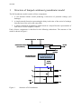
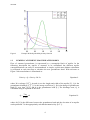
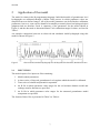
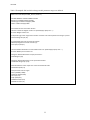
R-Groundwater: model user's
manual for NERC Virtual
Observatory implementation
Groundwater Science Programme
Open Report OR/11/059
Actual Evaporation Precipitation
Soil Moisture Model
(soil, landuse)
Runoff
FAO 56
Excess water
Potential recharge
Soil drainage spread over n months according to Weibull distribution
Unsaturated Zone Transfer function
Actual recharge
Kw
Qw
hw
Kp
hp
Qp
S
Ka
z
ha
Qa
BRITISH GEOLOGICAL SURVEY
GROUNDWATER SCIENCE PROGRAMME
OPEN REPORT OR/11/059
R-Groundwater: model user's
manual for NERC Virtual
Observatory implementation
The National Grid and other
Ordnance Survey data are used
with the permission of the
Controller of Her Majesty’s
Stationery Office.
Licence No:100017897/2007.
C R Jackson and L Wang
Keywords
Lumped groundwater model; R
code; NERC Virtual
Observatory;.
Front cover
Structure of R-Groundwater
model.
Bibliographical reference
JACKSON, C R AND WANG, L.
2011. R-Groundwater: model
user's manual for NERC Virtual
Observatory implementation.
British Geological Survey Open
Report, OR/11/059. 19pp.
Copyright in materials derived
from the British Geological
Survey’s work is owned by the
Natural Environment Research
Council (NERC) and/or the
authority that commissioned the
work. You may not copy or adapt
this publication without first
obtaining permission. Contact the
BGS Intellectual Property Rights
Section, British Geological
Survey, Keyworth,
e-mail [email protected]. You may
quote extracts of a reasonable
length without prior permission,
provided a full acknowledgement
is given of the source of the
extract.
Maps and diagrams in this book
use topography based on
Ordnance Survey mapping.
© NERC 2011. All rights reserved
Keyworth, Nottingham British Geological Survey 2011
BRITISH GEOLOGICAL SURVEY
The full range of our publications is available from BGS shops at
Nottingham, Edinburgh, London and Cardiff (Welsh publications
only) see contact details below or shop online at
www.geologyshop.com
The London Information Office also maintains a reference
collection of BGS publications including maps for consultation.
The Survey publishes an annual catalogue of its maps and other
publications; this catalogue is available from any of the BGS Sales
Desks.
The British Geological Survey carries out the geological survey of
Great Britain and Northern Ireland (the latter as an agency
service for the government of Northern Ireland), and of the
surrounding continental shelf, as well as its basic research
projects. It also undertakes programmes of British technical aid in
geology in developing countries as arranged by the Department
for International Development and other agencies.
The British Geological Survey is a component body of the Natural
Environment Research Council.
British Geological Survey offices
BGS Central Enquiries Desk
 0115 936 3143
email [email protected]
Fax 0115 936 3276
Kingsley Dunham Centre, Keyworth, Nottingham NG12 5GG
 0115 936 3241
Fax 0115 936 3488
email [email protected]
Murchison House, West Mains Road, Edinburgh EH9 3LA
 0131 667 1000
Fax 0131 668 2683
email [email protected]
London Information Office, Natural History Museum,
Cromwell Road, London SW7 5BD
SW7 2DE
 020 7589 4090
Fax 020 7584 8270
 020 7942 5344/45
email [email protected]
Columbus House, Greenmeadow Springs, Tongwynlais,
Cardiff CF15 7NE
 029 2052 1962
Fax 029 2052 1963
Forde House, Park Five Business Centre, Harrier Way,
Sowton EX2 7HU
 01392 445271
Fax 01392 445371
Maclean Building, Crowmarsh Gifford, Wallingford
OX10 8BB
 01491 838800
Fax 01491 692345
Geological Survey of Northern Ireland, Colby House,
Stranmillis Court, Belfast BT9 5BF
 028 9038 8462
Fax 028 9038 8461
www.bgs.ac.uk/gsni/
Parent Body
Natural Environment Research Council, Polaris House,
North Star Avenue, Swindon SN2 1EU
Fax 01793 411501
 01793 411500
www.nerc.ac.uk
Website www.bgs.ac.uk
Shop online at www.geologyshop.com
OR/11/059
Contents
1
Structure of lumped catchment groundwater model
1.1 Soil moisture balance model
1.2 Unsaturated zone transfer function
1.3 Lumped catchment groundwater model
1
2
3
4
2
Application of the model
2.1 Input files
7
7
References
13
FIGURES
Figure 1
Structure of R-Groundwater ............................................................................... 1
Figure 2
Example Weibull probability density function .................................................. 4
Figure 3
Basic structure of lumped catchment groundwater model ................................. 5
Figure 4
Example lumped groundwater model structure for application to a Chalk
aquifer................................................................................................................. 6
Figure 5
Observed and simulated hydrograph for the Baydon Hole borehole, Berkshire
Downs................................................................................................................. 7
TABLES
Table 1
Summary of model parameters .......................................................................... 8
Table 2
Format of main input file “Input.txt” ................................................................. 9
Table 3
Format of observed groundwater level input file ............................................. 10
Table 4
Format of rainfall and PE input file ................................................................. 10
Table 5
Example R file in which recharge model parameter ranges are defined .......... 11
Table 6
Example R file in which groundwater model parameter ranges are defined ... 12
i
OR/11/059
Summary
This report describes the structure and usage of the R-Groundwater model for implementation
within the NERC Virtual Observatory project. R-Groundwater is a simple lumped catchment
groundwater model written in the R programming language and run within the R
environment. It has been developed to model groundwater level time series at observation
boreholes by linking simple algorithms to simulate soil drainage, the transfer of water through
the unsaturated zone and groundwater flow. Time-series of flow through the outlets of the
groundwater store are also generated, which can be related to river flow measurements.
The model is calibrated through a Monte Carlo process by randomly selecting input parameter
values from ranges specified by the user. Simple text files are used to define the input to the
model and to write the output.
ii
OR/11/059
1
Structure of lumped catchment groundwater model
The R-Groundwater model consists of three components:
1. A soil moisture balance model producing a time-series of potential recharge (soil
drainage).
2. A simple transfer function representing the delay in the time of the arrival of recharge
from the base of the soil to the water table.
3. A lumped catchment groundwater model based on a simple Darcian representation of
flow out of a series of aquifer “outlets”.
Each of these components is described in the following subsections. The structure of the
model is shown in Figure 1.
Actual Evaporation Precipitation
Soil Moisture Model
(soil, landuse)
Runoff
FAO 56
Excess water
Potential recharge
Soil drainage spread over n months according to Weibull distribution
Unsaturated Zone Transfer function
Actual recharge
Kw
Qw
hw
Kp
hp
Qp
S
Ka
z
Qa
ha
Figure 1
Structure of R-Groundwater
1
OR/11/059
1.1
SOIL MOISTURE BALANCE MODEL
Potential recharge from the base of the soil zone is calculated using the FAO method (FAO,
1998), which describes soil moisture as a function of both vegetation root depth, and the
propensity of vegetation to withdraw available water from the soil. Thus, this approach can
appropriately represent soil moisture response to contrasting land-cover types.
In the FAO method, soil moisture is calculated using a maximum root depth (Zr), and
moisture depletion fraction (dp) parameter, which varies between vegetation and soil types.
The amount of water available to plants after a soil has drained to its field capacity, is
described as the total available water (TAW). TAW is defined as a function of the field
capacity (FC), wilting point (WP) and maximum root depth (Zr) such that:
TAW  Z r FC  WP 
Equation 1
As the moisture content of the soil column decreases, vegetation will find it more difficult to
extract moisture from the soil matrix. The fraction of TAW that can easily be extracted before
this point, is reached is described as readily available water (RAW). The value of RAW is
related to TAW by a land-cover defined depletion factor (dp):
RAW = dp TAW
Equation 2
where Rf is the rainfall and SMD is the soil moisture deficit. The intermediate soil moisture
deficit, SMD ' , is then:
SMD '  SMD  t 1  PE ' Rf
Equation 3
where PE ' is the potential evaporation. If in the above calculation SMD drops below RAW,
the evaporation, AE, will take place at a lower rate determined by the equation:
 TAW  SMD`
AE  PE ' 

 TAW  RAW 
0.2
when SMD` > RAW
Equation 4a
AE  PE '
when SMD` ≤ RAW
Equation 4b
AE  0
when SMD`  TAW
Equation 4c
The calculation of SMD at the end of each timestep is then made with respect to the above,
such that:
SMD( t )  SMD' AE  PE '
Equation 5
2
OR/11/059
The excess water (EXW), or the amount of water that is available for surface runoff and
potential groundwater recharge, is calculated as the amount of precipitation remaining after
losses through interception, evapotranspiration, and soil moisture replenishment, such that:
EXW  Rf  AE  (SMD ( t 1)  SMD ( t ) )
when SMD  0
Equation 6a
EXW  SMD
when SMD < 0
Equation 6b
The potential recharge, PR, is then calculated as:
PR  BFI  EXW
Equation 7
where BFI is the baseflow index. The parameters for FAO method can be based on those
given in the FAO Irrigation and Drainage Paper 56 (FAO, 1998).
1.2
UNSATURATED ZONE TRANSFER FUNCTION
A commonly applied transfer function as used by Calver (1997) is the basis for the transfer of
potential recharge from the base of the soil zone through the unsaturated zone to the water
table. Potential recharge from the base of the soil in each month is applied to the water table
over the current month and a number of subsequent months. The total number of months, n,
over which recharge is distributed is a model parameter.
The distribution of recharge over the n months is specified using a two-parameter Weibull
probability density function:
 k  x  k 1  x /  k
   e
 
f x ;  , k     
0


x 0,
Equation 8
x 0,
where k > 0 is the shape parameter and λ >0 is the scale parameter of the distribution. The
resulting distribution is scaled such that the area under the curve is equal to unity and
consequently the recharge for each time-step is simply spread over the selected, n, number of
months. This Weibull function can represent exponentially increasing, exponentially
decreasing, and positively and negatively skewed distributions as illustrated in Figure 2. It is
used because it is smooth and considered to be more physically justifiable than randomly
selected monthly weights.
3
OR/11/059
Figure 2
1.3
Example Weibull probability density function
LUMPED CATCHMENT GROUNDWATER MODEL
Flow of saturated groundwater is represented by a rectangular block of aquifer. In the
following description the aquifer is assumed to be unconfined but different aquifer
conceptualisations can easily be accommodated. A simple, explicit mass balance calculation
is performed at each time-step to calculate the new groundwater head. With reference to
Figure 3 this mass balance is formulated as:
R x y  Q  S x y  h / t
Equation 9
where R is recharge [LT-1], Δx and Δy are the length and width of the aquifer [L], Q is the
groundwater discharge [L3T-1], S is the storage coefficient [-], δh is the change in groundwater
head [L] over time, δt [T] and h is the groundwater head [L]. The discharge term, Q, is
calculated using an equation of the form:
Q
T y
h
0.5x
Equation 10
where Δh [L] is the difference between the groundwater head and the elevation of an aquifer
outlet point and T is the appropriately calculated transmissivity [L2T-1].
4
OR/11/059
R Q h Dy Dx Figure 3
Basic structure of lumped catchment groundwater model
Groundwater flow out of the aquifer is split into a series of discharges via outlets at different
elevations. Each of these outlets is associated with a vertical section of aquifer to which a
value of hydraulic conductivity is specified (Figure 4). The aquifer is drained by a stream with
perennial (Qp) and intermittent (Qw) flow components. A third discharge component (Qa) is
added at the base of the system to represent groundwater discharge below the level of a
perennial stream. The groundwater level may fall beneath the level of the perennial stream
(hp) but will always be above the base of the aquifer (Zb).
Hydraulic conductivity is defined using three piecewise constant values. The section of the
aquifer discharging to the intermittent stream (above hw) is characterised by hydraulic
conductivity, Kw. The perennial stream is fed by a zone with hydraulic conductivity, Kp; and
the groundwater discharge zone (below hp) is controlled by a hydraulic conductivity, Ka. The
storativity of the aquifer is depth invariant.
The discharge terms, Q, are again calculated using Equation 3 where Δh [L] is the difference
between the groundwater head and the elevation of the outlet below, or the difference in
elevation between two outlets, depending on the current groundwater head, and T is the
appropriately calculated transmissivity [L2T-1].
5
OR/11/059
R
Kw
Qw
hw
Kp
hp
Qp
S
Ka
Qa
ha
z
Figure 4
Example lumped groundwater model structure for application to a Chalk aquifer
6
OR/11/059
2
Application of the model
The model is written in the R programming language. Individual models of groundwater level
hydrographs are calibrated through a Monte Carlo process in which parameter values are
sampled from user defined ranges. All of the model parameters can be defined as calibration
parameters, however, some can be identified reasonably accurately based on hydrogeological
judgment and are therefore fixed. A summary of the parameters for the model shown in
Figure 4, and the data used to determine Monte Carlo calibration ranges for them, are listed in
Table 1.
An example comparison between an observed and simulated chalk hydrograph using this
model is shown in Figure 5.
Figure 5
2.1
Observed and simulated hydrograph for the Baydon Hole borehole, Berkshire Downs.
INPUT FILES
The model requires five input text files containing:
1. Model control parameters.
2. A times series of observed groundwater levels against which the model is calibrated.
3. Time-series of rainfall and potential evaporation.
4. An R file in which parameter value ranges for the soil moisture balance model and
recharge transfer function are specified.
5. An R file in which parameter value ranges for the saturated groundwater model
component are specified.
The format of these files is presented in Table 2 to Table 6.
7
OR/11/059
Table 1 Summary of model parameters
Saturated zone
Unsaturated
zone
transfer
Soil moisture
balance
Model
component
Parameter
Data informing parameter estimation
Runoff coefficient, RO
River base flow indices (1-BFI).
Field capacity, FC
FAO Irrigation and Drainage paper 56 (FAO 1998).
Wilting point , WP
FAO Irrigation and Drainage paper 56 (FAO 1998).
Maximum rooting depth, Zr
FAO Irrigation and Drainage paper 56 (FAO 1998).
Depletion factor, dp
FAO Irrigation and Drainage paper 56 (FAO 1998).
Number of months over which to distribute
potential recharge, n
Cross-correlation of monthly groundwater levels and lagged monthly rainfall.
Weibull shape parameter, k
Calibration parameter but varied between values that allows a broad range of distributions to be tested.
Weibull shape parameter, 
Calibration parameter but varied between values that allows a broad range of distributions to be tested.
Elevation of intermittent stream outlet, hw
DTM elevation of intermittent streams.
Elevation of Perennial stream outlet, hp
DTM elevation of perennial streams.
Elevation of groundwater discharge outlet,
ha
Geological and hydrogeological boreholes logs.
Hydraulic conductivity, of upper aquifer
(above hw), Kw
Calibration ranges based on pump test data and hydrogeological experience.
Hydraulic conductivity, of middle aquifer
(between hw and hp), Kp
Calibration ranges based on pump test data and hydrogeological experience.
Hydraulic conductivity, of lower aquifer
(between hp and ha), Ka
Calibration ranges based on pump test data and hydrogeological experience.
Storativity of aquifer, S
Calibration ranges based on pump test data and hydrogeological experience.
8
OR/11/059
Table 2 Format of main input file “Input.txt”
Line 1 2 3 4 5 6 7 8 9 10 11 12 13 14 15 16 17 18 19 20 21 22 23 24 25 26 27 28 29 30 31 File contents
‐‐‐‐ Using the output from a previous run? (Y or N)
N ‐‐‐‐ If Y, run all behavioural models (i.e. that met error criterion)? (Y or N) N ‐‐‐‐ If N, specify the number of best models to be used? 10 ‐‐‐‐ Recharge parameter input R file name Recharge_Model_Parameters.txt ‐‐‐‐ Groundwater parameters input R file name? Groundwater_Model_Parameters.txt ‐‐‐‐ Simulation start end date (format DD‐MM‐YYYY) 15/01/1970 15/12/1989 ‐‐‐‐ Initial groundwater level 16.8175 ‐‐‐‐ Number of Monte Carlo calibration runs 1000000 ‐‐‐‐ Rainfall and PE data file name Rainfall_PE.txt ‐‐‐‐ Groundwater level file name Groundwater_levels.txt ‐‐‐‐ Input directory E:\NERC_VO_VERSION\ ‐‐‐‐ Output directory E:\NERC_VO_VERSION\Results\ ‐‐‐‐ Run name Example ‐‐‐‐ Error measure flag: 1=RMSE, 2=COREL, 3=RMSE of extreme values, 4=NSE 1 ‐‐‐‐ Error measure value (only those meeting criterion are stored) 1.7 9
Description Comment line
Flag to determine if running previously calibrated models Comment line Flag to determine if should re‐run all behavioural models Comment line If re‐running subset of behavioural models how many should be run? Comment line Name of recharge model parameter input file Comment line Name of recharge model parameter input file Comment line Simulation start date in dd/mm/yyyy format Simulation end date in dd/mm/yyyy format Comment line Initial groundwater head (m) Comment line Number of simulations in Monte Carlo run Comment line Name of rainfall and PE input file Comment line Name of input file containing observed groundwater levels Comment line Input directory path Comment line Output directory path (must exist before model is run) Comment line Name of run which forms start of output file names Comment line Flag specifying which error measure to use Comment line Error measure limiting criterion value for identifying behavioural models OR/11/059
Table 3 Format of observed groundwater level input file
File contents dt gwl 1970‐01‐15 16.82 1970‐02‐15 20.88 1970‐03‐15 22.40 1970‐04‐15 21.81 1970‐05‐15 21.91 1970‐06‐15 20.66 1970‐07‐15 19.46 1970‐08‐15 17.96 1970‐09‐15 16.68 1970‐10‐15 15.46 1970‐11‐15 14.28 1970‐12‐15 13.75 1971‐01‐15 14.39 1971‐02‐15 16.18 1971‐03‐15 19.42 etc Description Header containing string “dt gwl”
Date in yyyy‐mm‐dd format and groundwater level A space separated file Table 4 Format of rainfall and PE input file
File contents dt pptn pe 1970‐01‐15 72.0 12.0 1970‐02‐15 70.9 24.2 1970‐03‐15 65.0 40.6 1970‐04‐15 43.3 56.2 1970‐05‐15 90.8 82.8 1970‐06‐15 10.4 85.6 1970‐07‐15 14.0 92.8 1970‐08‐15 96.9 77.2 1970‐09‐15 52.3 61.4 1970‐10‐15 22.5 44.1 1970‐11‐15 46.0 26.4 1970‐12‐15 124.0 12.4 1971‐01‐15 47.6 11.0 etc Description Header containing string “dt pptn pe”
Date in yyyy‐mm‐dd format followed by rainfall (mm) and PE (mm) A space separated file 10
OR/11/059
Table 5 Example R file in which recharge model parameter ranges are defined
# Name of rainfall file? Change the name inside the ""
df.Rain.File=read.table("Rainfall_PE.txt",header=T) # DO NOT MODIFY THE FOLLOWING 3 LINES dt.Date.In=as.POSIXct(df.Rain.File$dt) nu.Recharge.In=df.Rain.File$pptn/1000 nu.PE.In=df.Rain.File$pe/1000 # Parameters for the UZ transfer funtion # Are the number of weights random or specfied (S/R)? (keep the " ") ch.Calver.Weights.Choice="R" # If R (random) give the range of the number of months over which potential recharge is spread nu.Calver.Range.U=c(12,12) # If S (specified) then give the monthly weights # Monthly weights for transfer function (u) nu.U=c(0.2,0.4,0.3,0.1) # Are the Weibull distribution k and lambda random or specfied (S/R)? (keep the " ") ch.Calver.Weibull.param.Choice="S" # Range for Weibull distribution shape parameter k nu.Wk.Range=c(2,6) # Range for Weibull distribution scale parameter lambda nu.Wlambda.Range=c(1.8,3.0) # Runoff coefficient value equals one minus the base flow index nu.ROCoeff=c(0.01,0.3) # Soil parameter values ranges nu.FC=c(0.2904,0.2904) nu.WP=c(0.1529,0.1529) nu.Zr=c(0.5,1.3) nu.dp=c(0.02,0.2) nu.SMDStart=c(0.0,0.0) nu.PEAEFrac=c(0.1,0.1) 11
OR/11/059
Table 6 Example R file in which groundwater model parameter ranges are defined
#‐‐‐‐‐‐‐‐‐‐‐‐‐‐‐‐‐‐‐‐‐‐‐‐‐‐‐‐‐ # SET PARAMETER RANGES BY CHANGING VALUES WITHIN c( , ) # Length of aquifer nu.Length=c(4408,4408) # Kw ‐ Hydraulic conductivity for heads > Hw nu.K.High=c(30,50) # Kp ‐ Hydraulic conductivity for heads > Hp nu.K.Low=c(30,45) # Ka ‐ Hydraulic conductivity for < Hp nu.K.Base=c(0.02,0.2) # S ‐ Storage coefficient nu.S.Low=c(0.01,0.03) # Ha ‐ Base elevation of the aquifer nu.H.Low=c(‐46,‐46) # Hp ‐ Outlet elevation for perennial river nu.H.Mid=c(4,8) # Hw ‐ Outlet elevation for ephemeral river nu.H.High =c(6,23.5) #‐‐‐‐‐‐‐‐‐‐‐‐‐‐‐‐‐‐‐‐‐‐‐‐‐‐‐‐‐ # DO NOT ALTER DATA BELOW HERE # Dummy variables nu.T.Low=c(10,500) nu.T.High=c(500,5000) nu.S.High=c(0.003,0.003) nu.H.Mid2=c(120,140) 12
OR/11/059
References
CALVER A. 1997. Recharge Response Functions. Hydrology and Earth System Sciences 1: 47-53.
FAO, 1998. Crop evapotranspiration; guidelines for computing crop water requirements, FAO
Irrigation and Drainage Paper 56, Rome, 301pp.
13