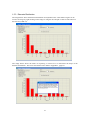
1
Software to support Forestry Commission Information Note 45 ‘Monitoring the Transformation of Even-aged Stands to Continuous Cover Management’ User Manual Gary Kerr and Dan Johnson with help and support from: Geoff Morgan, Una McEvoy, Victoria Stokes and Anna Brown. August 2004 Forestry Commission Research Agency Alice Holt Lodge Wrecclesham Farnham Surrey GU10 4LH Tel: 01420 22255 e-mail: [email protected] 1 Contents Page No. Background and Introduction Program Input Program Outputs Structure of the User Guide Installing the Program Running the Program Help and Advice 1.0 2.0 4 4 4 5 5 5 6 Understanding the User Interface 7 1.1 Main Window 1.1.1 Main Workspace 1.1.2 Menu Options 1.1.3 Tool Buttons 1.1.4 General Tips on Navigation and Using Lists 7 7 8 9 10 1.2 Select Stand Window 12 1.3 The Stand Manager Window 1.3.1 Tab Sheets in the Stand Manager Window 13 14 1.4 Windows Relating to Monitoring Assessments 1.4.1 The Monitoring Assessment Tab Sheet 1.4.2 The Monitoring Assessment Window 1.4.3 The Monitoring Plot Window 1.4.4 The Monitoring Species Window 15 15 16 18 20 1.5 The Report Window 1.5.1 Number and Size of Trees 1.5.2 Basal Area per Hectare 1.5.3 Diameter Distribution 1.5.4 Number of Saplings per Hectare 1.5.5 Number of Seedlings per Hectare 1.5.6 Vegetation Type 22 24 26 27 28 30 32 1.6 Windows Relating to Ancillary Monitoring Information 1.6.1 The Stand Position Tab Sheet 1.6.2 The Diary Entry Tab Sheet 1.6.3 The Diary Entry Window 1.6.4 The Fixed Point Tab Sheet 1.6.5 The Fixed Point Window 1.6.6 The Image Window 1.6.7 The Transformation Plan Tab Sheet 33 33 34 35 36 37 38 39 Step-by-Step Guide 40 2.1 40 40 40 Creating New Stands and Saving Information 2.1.1 Creating a New Stand 2.1.2 Saving Stand Details to the Database 2 3.0 2.2 Opening and Editing an Existing Stand 41 2.3 Deleting One or More Stands 41 2.4 Inputting and Editing Monitoring Assessments 2.4.1 Adding a New Monitoring Assessment 2.4.2 Editing/Viewing an Existing Monitoring Assessment 2.4.3 Deleting Existing Monitoring Assessments 2.4.4 Adding Plots to a Monitoring Assessment 2.4.5 Editing/Viewing a Monitoring Plot 2.4.6 Deleting Plots from a Monitoring Assessment 2.4.7 Adding Species to a Monitoring Plot 2.4.8 Editing/Viewing a Monitoring Species 2.4.9 Deleting Species from a Monitoring Plot 2.4.10 Amending Vegetation Cover Data for a Monitoring Plot 42 42 43 43 44 44 45 45 46 46 47 2.5 Output of Monitoring Data to Microsoft Excel 97 and Word 97 2.5.1 Example Output of Tables and Figures 49 51 2.6 52 Saving an image from the report window to File Inputting and Editing Ancillary Monitoring Information 53 3.1 Working with Diary Entries 3.1.1 Adding Diary Entries 3.1.2 Editing and Viewing Diary Entries 3.1.3 Deleting Diary Entries 53 53 53 53 3.2 Working with Fixed Points and Fixed Point Photographs 3.2.1 Adding Fixed Points 3.2.2 Editing Fixed Points 3.2.3 Deleting Fixed Points 3.2.4 Adding Photographs 3.2.5 Viewing Photographs 3.2.6 Deleting Photographs 54 54 54 55 55 56 56 3.3 Working with Transformation Plans 3.3.1 Adding Transformation Plans 3.3.2 Deleting Transformation Plans 56 56 57 References 58 Appendices 59 Appendix 1: Skewness in the diameter distribution Appendix 2: Index for clustering for saplings and seedlings Appendix 3: National reference system of Great Britain Appendix 4: File Share Utility User Manual 3 59 61 63 64 Background and Introduction Since the early 1980s continuous cover forestry (CCF) has featured increasingly in discussions about the future management of British forests (Mason et al., 1999). For example, ‘The UK Forestry Standard’ (Forestry Commission, 1998) requires managers to ‘identify areas which are, or will be, managed under a continuous cover forestry system and build them into the forest design’. In addition, ‘Woodlands for Wales’ (Forestry Commission, 2001) commits the Forestry Commission to convert at least half state owned woodlands in Wales to continuous cover over the next 20 years. Guidance on silvicultural options for transformation of an even-aged stand to continuous cover is given in Forestry Commission Information Note 40 (Mason and Kerr, 2001). This focussed attention on the fact that a prerequisite for the successful adoption of CCF is a commitment to a more flexible, adaptive approach to stand management based on an understanding of woodland development over time in a given location. As a further development, and in response to the requirements of forest managers, a system of sampling to monitor the process of transformation has been developed and is described in Forestry Commission Information Note 45 (Kerr et al., 2002). The main skill of transformation is manipulating the current stand in such a way that a successor stand is initiated and then developed with time. Following from this the system of sampling aims to: (i) to quantify the basal area, diameter distribution and species composition of a stand, and (ii) assess existing regeneration, and using information on browsing impacts and vegetation, produce information on the possible receptivity of the site to further regeneration. To further support forest managers who use this monitoring system we have developed this software. The program aims to provide a convenient method of processing the data into a format that will help understand what is happening in the stand, this can then be used as a basis to plan future silvicultural interventions. The opportunity has also been taken to allow other information concerning the transformation of an area to be recorded alongside the monitoring data. Hence the system allows the transformation plan, diary notes, fixed-point photographs and information on stand location to be stored. Supported operating systems include Windows NT/2000/XP. Program Input At present the system uses data that have been entered directly into the system. However, future versions could input data via a number of specialised user-interfaces, including hand-held data-capture devices. All data are stored in database files. Program Outputs A Microsoft Excel 97 workbook of summary tables and figures that are seen on-screen while using the software. A Word document summary of the selected stand assessment. 4 Structure of the User Guide The document has been split into three parts. 1. Understanding the User Interface: page 7 This section provides a short tour around the various interfaces and gives a brief description of the purpose of the on-screen components. It is recommended that this section is read before attempting to use the system. 2. Step by Step Guide: page 40 This section gives specific instructions on how to perform standard tasks. 3. Appendices page 60 These contain more detailed information on the statistical tests used in the software and the National referencing system of Great Britain. Appendix 4 is a guide for the File Share Utility that will only be distributed to selected users only. Installing the program Insert the FCIN45 Installation CD into your CD drive. • • • • • • Click on the Start Menu. Click on the Run option. Type <drive>:\setup.exe (where <drive> is the letter corresponding to your CD drive). Press the OK button. Follow all on-screen instructions. Restart your PC following completion. Running the program Click on the Start Menu. Click on All Programs/Programs (depending on your operating system). Highlight the FCIN45 folder. Click on the FCIN45 application shortcut. 5 Help and advice We hope you find this software useful and welcome feedback on it and any observations and experience you have of continuous cover forestry in Britain. Gary Kerr or Victoria Stokes Alice Holt Lodge Farnham Tel: 01420 22255 [email protected] [email protected] Bill Mason or Colin Edwards Northern Research Station Roslin Tel: 0131 445 2176 [email protected] [email protected] 6 1.0 Understanding the User Interface The user interface can be divided into six main parts. • The Main Window (see 1.1) which gives access to most of the generic functions of the program. • The Select Stand Window (see 1.2) which allows stands to be selected for viewing or deletion. • The Stand Manager Window (see 1.3) which sets up stand to hold monitoring data. • Windows Relating to Monitoring Assessments (see 1.4). • The Report Window (see 1.5) • Windows Relating to Ancillary Monitoring Information (see 1.6), such as fixed point photographs, transformation plans, stand position and diary entries. Throughout the guide a window is denoted using underline, e.g. Main Window and elements of each window are italicised, e.g. main workspace. 1.1 Main Window When the program runs the first window to show is the Main Window, as shown below. Helpful hints 1.1.1 Main Workspace This is where all Windows will be displayed. 7 1.1.2 Menu Options File Menu (Keyboard Shortcut : Alt+F) New Clicking this menu option will create a new stand. Keyboard Shortcut : CTRL+N Load Displays a list of existing stands in the Select Stand Window. Keyboard Shortcut: CTRL+L Edit Opens the selected record for editing. Keyboard Shortcut: CTRL+E Delete Deletes the selected record. Keyboard Shortcut: Delete Save Clicking this menu option will save the current stand and all associated information. Keyboard Shortcut: CTRL+S Quit Exits the program. Keyboard Shortcut: CTRL+Q Edit Menu (Keyboard Shortcut: Alt+E) Cut Copies selected text to the clipboard and removes it from the selected control. Keyboard Shortcut: CTRL+X Copy Copies selected text to the clipboard. Keyboard Shortcut: CTRL+C Paste Pastes the contents of the clipboard into the selected control. Keyboard Shortcut: CTRL+V Print Menu (Keyboard Shortcut: Alt+P) Print To Excel Prints all the selected assessment to an Excel spreadsheet. If used from the Monitoring Information Window, it will copy the plot data. If used from the Report Window, it will copy the selected table details. Keyboard Shortcut: CTRL+P Print To Word Prints a summary report of the selected stand to a Word document. Only operable from the Report Window. Keyboard Shortcut: CTRL+C Paste Pastes the contents of the clipboard into the selected control. Keyboard Shortcut: CTRL+V Help Menu (Keyboard Shortcut: Alt+H) About Displays the About Window detailing product name and version information. Keyboard Shortcut: CTRL+A 8 1.1.3 Tool Buttons The tool buttons all have the same functionality as the menu options described in the previous section. They are listed below. New CTRL+N Creates a new record Load CTRL+L Lists the available stands Edit CTRL+E Edits the selected record Delete Delete Deletes the selected record from memory Save CTRL+S Saves the entire stand to the database Quit CTRL+Q Quits the application Cut CTRL+X Cuts selected text to the clipboard Copy CTRL+C Copies selected text to the clipboard Paste CTRL+V Pastes selected text from the clipboard Print to Excel CTRL+P Prints the current assessment to Excel Print to Word CTRL+W Prints the current assessment to Word About CTRL+A Displays program information Save Graph/Chart to File CTRL+G Saves the graph or chart image currently displayed by the Report form to a bitmap file. File Share Utility CTRL+F Loads the File Share Utility –Selected users only 9 1.1.4 General Tips on Navigation and Using Lists Navigating Between Windows Esc Closes the current window and discards any changes made to it. Enter Closes the current window and applies any changes made to it Note that with the exception of the Stand Manager Window, these changes are not saved to the database until the stand is saved. Navigation Within a Window Tab Moves to the next control within a window. Note that it is not possible to tab onto the buttons. However, they all have keyboard shortcuts which can be used instead of the mouse. Shift+Tab Moves to the previous control within a window. Right Arrow Moves to the next cell in the DBH grid and commits the value entered in the current cell. Moves between menus. Moves to the next tab sheet. Left Arrow Moves to the previous cell in the DBH grid and commits the value entered in the current cell. Moves between menus. Moves to the previous tab sheet. Up Arrow Moves to the previous item in a list. Down Arrow Moves to the next item in a list. Selecting Items in a List 1. Selecting one item Highlight the item by left-clicking on it with your mouse. Or use the up down arrow keys on your keyboard until the item you want is highlighted in blue. 2. Selecting Multiple adjacent items Select the first item in the group as described above. Either press Shift+Up/Down to select the remaining items. Or drag the mouse across all items to be selected. 3. Selecting Multiple Items that are not Adjacent Select one item as described above. Hold down the Ctrl key and select the remaining stands one by one using your mouse. 10 Note: Not all lists facilitate multiple selection. Selecting Vegetation Types in the Vegetation Check List Navigate through the list using the up/down arrows on the keyboard, press the number of the item you wish to navigate to, or just use your mouse. Check or uncheck the checkbox corresponding to the highlighted item by pressing the space bar once or left click on the item with your mouse. Selecting Species from the Species List Box Either follow the steps for ‘Selecting one item’ from the section ‘Selecting Items in a List’. Or enter the first letter of the species you wish to select, the use the up/down arrow keys until the required species name is displayed. 11 1.2 The Select Stand Window The image below shows the Select Stand Window. To select one stand: Highlight it by left-clicking on it with your mouse or by using the up down arrow keys on your keyboard. To select multiple adjacent stands: Select the first stand in the group as described above. Then press Shift+Up/Down to select the remaining stands, or drag the mouse across all stands to be selected. To select mulitple stands that are not adjacent: Select one stand as described above. Then hold down the Ctrl key and select the remaining stands one by one using your mouse. The Esc key on your keyboard returns you to the Main Window. Edit Button (CTRL+E) Opens the selected stand to view or edit; only one stand may be opened for editing at any given time. Delete Button (Delete) Click Delete or use the Delete key on your keyboard to delete selected stands. Warning: This operation cannot be reversed or cancelled. All selected stands will be permanently deleted from your database. You will however be prompted for confirmation before the delete operation proceeds. 12 1.3 Stand Manager Window If you are creating a new stand the next window after the Main Window is the Stand Manager Window. However, if you are opening an existing stand you will first need to select one in the Select Stand Window (shown on the previous page). The images below highlight the main parts of the Stand Manager Window. Forest Name Box Allows the name of the forest to be input/displayed Compartment Name Box Allows the number or name of the compartment to be input/displayed. Compartment Size Box Allows the size of the compartment to be input/displayed. Note: This value is not used in any calculations, most of which are per hectare. Stand Name Box Allows the unique stand name to be input/displayed. This is the name you see in the Select Stand Window after File|Open (see below). Note, if the box is left blank a default name will be created. OK Button Saves all changes made to the stand to the database and closes the 13 Stand Manager Window. Cancel Button Discards all changes made to the stand since the last save and closes the Stand Manager Window. 1.3.1 Tab-sheets in the Stand Manager Window Within the Stand Manager Window there are five tab sheets that give access to other parts of the program. The first is the Monitoring Assessment tab sheet, which allows data to be input and edited (see 1.4.1). It also gives access to the report facility (see 1.5). The other four tab-sheets are Stand Position, Diary Entry, Fixed Point and Transformation Plan. These all allow ancillary information to be stored alongside the monitoring data and are described in section see 1.6. 14 1.4 Windows Relating to Monitoring Assessments 1.4.1 The Monitoring Assessment Tab Sheet The image below highlights the main parts of the Monitoring Assessment tab sheet. Existing Monitoring Assessment List Lists existing monitoring assessments for the selected stand. Note that before attempting to edit, delete or report a monitoring assessment must be selected. A record may be selected by either clicking on it once with the mouse, or tabbing to the list and then using the up/down arrows on the keyboard until the relevant record is highlighted in blue. New Monitoring Assessment Button (CTRL+N) Opens a blank Monitoring Assessment Window (see 1.4.2, page 16). Edit Monitoring Assessment Button (CTRL+E) Opens a Monitoring Assessment Window (see 1.4.2, page 16) showing the details of the selected record. Delete Monitoring Assessment Button (Delete) Deletes the currently selected Monitoring Assessment (BEWARE a lot of data can be lost this way. However, you will be prompted for confirmation before the delete operation proceeds. Note: The selected monitoring assessment is deleted from memory. However this change can be cancelled provided that it has not been saved to the database using the Save Button (CTRL+S). Monitoring Assessment Report Button (CTRL+R) Opens the Report Window (see 1.5, page 22). Once data is entered, this is the most useful facility in the system, it produces data summaries, performs statistical analysis if required and all tables and figures produced can be exported to Microsoft Excel and Microsoft Word (see 2.2, page 41) for inclusion in reports. 15 1.4.2 The Monitoring Assessment Window The Monitoring Assessment Window is used to add new or edit existing data. An Excel report containing all the data in the Grid of Existing Plots can also be created from within this window, using CTRL+P or the Print to Excel Button on the toolbar. The image below highlights the main parts of the screen. Assessment Date Box Displays the assessment date and facilitates its input using a calendar. Plot Area Box Allows the area (in hectares) of each plot to be specified and displayed. Distance Between Plots Box Allows the distance (in metres) between each plot to be specified. This is S, as described in paragraph 19 of FCIN45; however, please note this is a record of S and it is not used in any calculations. Assessors Box Allows the name or initials of the assessor(s) to be specified and displayed. 16 Plot Area for Saplings Box Allows the area (in hectares) of each plot for monitoring saplings to be specified and displayed. The box should only be filled in if the plot area for saplings and seedlings was different to that for trees, see paragraphs 23-25 of FCIN45. Plots Are Permanent Checkbox The procedure described in FCIN45 allows permanent or temporary plots to be installed. However, this tick-box has no influence on the statistics carried out in this version of the program but indicates that in future versions this may be changed. Grid of Existing Plots Lists existing plot records. Before attempting to edit or delete plots an existing record must be selected. To select a plot, either use the up/down arrows on your keyboard to select any line of the plot, or click on any line of the plot using your mouse. The selected line will then be highlighted in blue. When the window first opens, the first plot is always selected by default. New Plot Button (CTRL+N) Opens a blank Monitoring Plot Window (see 1.4.3, page 18). Edit Plot Button (CTRL+E) Opens a Monitoring Plot Window (see 1.4.3, page 18) showing the details of the selected record highlighted in the grid of existing plots. If no plot has been selected you will be prompted to select a plot before attempting to edit one. Delete Plot Button (Delete) Deletes the currently selected plot. If no plot has been selected you will be prompted to select a plot before attempting to delete one. Note: The selected plot is deleted from memory. However this change can be cancelled provided that it has not been saved to the database using the Save button (CTRL+S). OK Button (Enter) Applies all changes made to the monitoring assessment and closes the Monitoring Assessment Window. Note that changes are not saved to the database until the Save button is used (CTRL+S). Cancel Button (Esc) Discards all changes made to the monitoring assessment and closes the Monitoring Assessment Window. 17 1.4.3 The Monitoring Plot Window The Monitoring Plot Window is used to add new plot data or edit existing plot data. The image below highlights the main parts of the screen. In this window the species list and vegetation check list are independent. The species list displays all species for which data exists in this plot. The vegetation check list allows % cover for each component of the groups of vegetation to be entered and accords with those in Appendix 2 of FCIN45. Note that the percentage value entered for each vegetation type must be between 1 and 100. Species List Lists the species included in the current plot record. Before attempting to edit or delete data for a species an existing record must be selected. A species may be selected by clicking on it using the mouse, or by tabbing into the list box and using the up/down arrows on the keyboard. 18 Vegetation Check-list Indicates which vegetation types the plot contains. Multiple vegetation types may be selected. Either the mouse or the keyboard may be used to select or deselect vegetation type. To use the keyboard, first tab onto the vegetation check-list. Then use the up /down arrows on your keyboard until the relevant vegetation type has been highlighted in blue. To select/deselect that vegetation type, press the space bar once. To use your mouse, just click on the vegetation type you wish to select/deselect. Note: If deselecting the check box will clear. If selecting you will then be prompted to enter the percentage coverage for this vegetation type in the current plot. This value must be between 1 and 100. (See below). The ninth option in the vegetation check-list ‘other specified’ allows you to specify your own vegetation type. If this is selected a Vegetation Description input box (shown below) will appear after the percentage cover has been entered. This enables you to enter your description. A common use of this has been to record the amount of ‘deadwood’. Results will be easier to interpret if the same component has been recorded over the whole area. New Species Button (CTRL+N) Opens a blank Monitoring Species Window (see 1.4.4, page 20). Edit Species Button (CTRL+E) Opens a Monitoring Species Window (see 1.4.4, page 20) showing the details of the selected record. Delete species button (Delete) Deletes the selected species. Note: The selected species is deleted from memory. However this change can be cancelled provided that it has not been saved to the database using the Save button (CTRL+S). OK button (Enter) Applies all changes made to the current plot and closes the Monitoring Plot Window. Note that changes are not saved to the database until the Save button is used (CTRL+S). Cancel button (Esc) Discards all changes made to the monitoring plot and closes the Monitoring Plot Window. 19 1.4.4 The Monitoring Species Window The Monitoring Species Window is used to add data on number and size of trees, saplings and seedlings for each individual species in each plot, or to edit these data. The image below highlights the main parts of the screen. A quick way to move between the boxes on this sheet is to use the TAB key. Available Species List Allows the selection of one species name from a pre-determined list. Enter the first letter of the species or use the up/down arrows to navigate through the list. DBH Grid Allows up to 25 tree DBH measurements to be entered/displayed. Either use your mouse to click into a cell and then enter the data, or tab into the grid and enter the data. Press the right arrow on the keyboard to commit each new entry. The right/left arrow keys can also be used to navigate through the grid. The DBH can be suffixed with f=frame tree, c=coppice tree and m=marked tree (e.g. 10f, 25m or 20 43c). This allows different classes of trees to be shown separately in some of the Report Window functions described in section 1.5. Height Box This can be used to record height measurements but they are not used in any calculations (see paragraphs 26 and 27 of FCIN45). Total Saplings Box This allows the total number of saplings found within the plot to be entered/displayed. The number of saplings in this and the next two boxes can be divided into saplings of maiden origin or of coppice origin. This allows the two to be shown separately in the Report function described in section 1.5. The notation to use is: 7 This means 7 saplings of maiden origin 3c This means 3 saplings of coppice origin 2c4 This means 6 saplings of which 2 are from coppice. Total Saplings With Deer Damage Box This allows entry of the number of saplings recorded to show signs of deer damage. The value entered must not be more than the value entered in the total saplings box. Total Saplings With DBH >= 3cm Box This allows entry of the number of large saplings, i.e. those with a DBH greater than or equal to 3cm. The value entered must not be more than the value entered in the total saplings box. Total Seedlings Box This allows entry of a total number of seedlings found within the plot. Total Seedlings With Deer Damage Box This allows entry of the number of seedlings recorded to show signs of deer damage. The value entered must not be more than the value entered in the total seedlings box. OK Button Applies all changes made to the current species and closes the Monitoring Species Window. Note that changes are not saved to the database until the Save button is used (CTRL+S). Cancel Button Discards all changes made to the current species and closes the Monitoring Species Window. 21 1.5 The Report Window The report facility is accessible via the Stand Manager Window using the report button (see 1.4.1) Once data are input into the system the program can perform the following tasks: A Calculate the number of trees per hectare grouped by species and size class. B Calculate the basal area per hectare by species. C Show a diameter distribution and perform a statistical test to determine its general shape. D Calculate the number of saplings per hectare grouped by species, deer damage and size, and perform a statistical test to determine distribution. E Calculate the number of seedlings per hectare grouped by species and deer damage, and perform a statistical test to determine distribution. F Calculate the minimum, mean and maximum for each component of vegetation cover. Note: For all of the above, the number of decimal places can be varied between 0 and 2. For A, B and D, there is a split facility which allows data to be divided into frame/coppice/other. For A, D and E, 95% confidence intervals can be calculated to indicate the precision of the estimate of the mean. Report Outputs Each individual table generated in the Report Window can be printed to an Excel spreadsheet for use in written reports using the Print to Excel button (CTRL+P) on the toolbar. The entire report can be printed to a Word document using the Print to Word button on the toolbar (CTRL+W). The images of diameter distribution and vegetation cover can also be saved as images for inclusion in reports using the Save Graph or Chart to File button on the toolbar (CTRL+G). The image below highlights the main parts of the Report Window. 22 Select Summary Type List Allows a Report type to be selected from a pre-determined list. Each one of these is considered separately in sections 1.5.1 to 1.5.6. Summary Table Displays tabular data from the requested Report. Summary Graph Displays graphical data from the requested Report. Display To Decimal Places Box Allows the number of decimal places displayed in the Report table to be specified. Display All Splits Box Allows all results to be displayed in terms of the number of frame, coppice and marked trees. Table / Graph split bar Allows the space occupied by the Report table to be adjusted to suit the user’s requirements. Esc Closes the Report Window or the Statistics Window if it is being displayed. 23 1.5.1 Number and Size of Trees The image below shows a dataset with the number of decimals set at zero and introduces a stand (Wykeham 5307) that will be used to display most of the functions available in the Report Window. If the show 95% confidence interval box is checked then the Report table changes as shown below; the confidence intervals are added to the total number for each species and each size class. 24 Using another set of data for a stand (Rushmore 8) where frame trees were recorded, the effect of ticking the show splits box can be seen. The number of frame and other trees are shown for each combination of species/size class. Note that the Figure can be saved as an image by right-clicking on the image or using the Save Graph or Chart to File button on the tool bar (CTRL+G). 25 1.5.2 Basal Area per Hectare The screen below shows the basal area per hectare for Wykeham 5307, note that the decimal place facility has been set to two as some species were uncommon. 26 1.5.3 Diameter Distribution The image below shows the diameter distribution for Wykeham 5307. Note that the Figure can be saved as an image by right-clicking on the image or using the Save Graph or Chart to File button on the tool bar (CTRL+G). The image below shows the effect of requesting a statistical test to determine the shape of the diameter distribution. The test is described in more detail in Appendix 1, page 60. 27 1.5.4 Number of Saplings per Hectare This screen is shown below is for the stand Wykeham 5307. This is the same data but with 95% confidence intervals for each species. 28 This is also the same data showing the result of the statistical test on the sapling distribution. This test is explained in greater detail in Appendix 2, page 62. The screen below shows the use of the split facility for the stand Rushmore 8. 29 1.5.5 Number of Seedlings Per Hectare This screen is shown below for the stand Wykeham 5307. This is the same data but with 95% confidence intervals for each species. 30 This is also the same data showing the result of the statistical test on the seedling distribution, the test is the same one as with saplings and is explained in greater detail in Appendix 2, page 62. 31 1.5.6 Vegetation Type The image below shows the vegetation data for Wykeham 5307. Note that the Figure can be saved as an image by right-clicking on the image or using the Save Graph or Chart to File button on the tool bar (CTRL+G). 32 1.6 Windows Relating to Ancillary Monitoring Information 1.6.1 The Stand Position Tab Sheet The stand position tab-sheet allows entry of Easting and Northing co-ordinate values for the position of the stand. The system is the National reference system for Great Britain, i.e. four figure Eastings and four figure Northings (see Appendix 3, page 64). The image below highlights the main parts of the tab-sheet. Northing Box Easting Box Easting Box Allows the Easting co-ordinate of the stand to be specified. Northing Box Allows the Northing co-ordinate of the stand to be specified. 33 1.6.2 The Diary Entry Tab Sheet The diary entry tab sheet allows diary information to be added and existing entries to be edited or deleted. The image below highlights the main parts of the tab-sheet. New Diary Entry Button (CTRL+N Edit Diary Entry Button (CTRL+E Delete Diary Entry Button (Delete) Existing Diary Entry List Existing Diary Entry List Lists existing diary entries. Before attempting to edit or delete diary entries an existing record must be selected. A record may be selected by either clicking on it once with the mouse, or tabbing to the list and then using the up/down arrows on the keyboard until the relevant record is highlighted in blue. New Diary Entry Button (CTRL+N) Opens a blank Diary Entry Window where a new diary entry can be created. See below. Edit Diary Entry Button (CTRL+E) Opens a Diary Entry Window (see below) showing the details of the selected record. Delete Diary Entry Button (Delete) Deletes the currently selected diary entry. Note: The selected diary entry is deleted from memory. However this change can be cancelled provided that it has not been saved to the database using the Save button (CTRL+S). 34 1.6.3 The Diary Entry Window The Diary Entry Window is used to add new or edit existing diary entries. The image below highlights the main parts of the screen. Entry date box Allows the date at which the diary entry was made to be entered using a calendar. Diary Entry Text Area Allows the details of the diary entry to be entered. OK Button Applies all changes made to the diary entry and closes the Diary Entry Window. Note that changes are not saved to the database until the Save button is used (CTRL+S). Cancel Button Discards all changes made to the current diary entry and closes the Diary Entry Window. 35 1.6.4 The Fixed Point Tab Sheet The fixed point tab sheet allows fixed point photographs to be added, edited or deleted and their position recorded. The image below highlights the main parts of the tab sheet. New Fixed Point Button (CTRL+N) Edit Fixed Point Button (CTRL+E) Delete Fixed Point Button (Delete) Existing Fixed Point List Existing Fixed Point List Lists existing fixed points. Before attempting to edit or delete fixed points an existing record must be selected. A record may be selected by either clicking on it once with the mouse, or tabbing to the list and then using the up/down arrows on the keyboard until the relevant record is highlighted in blue. New Fixed Point Button (CTRL+N) Opens a blank Fixed Point Window (see below). Edit Fixed Point Button (CTRL+E) Opens a Fixed Point Window (see below) showing the details of the selected record. Delete Fixed Point Button (Delete) Deletes the currently selected fixed point. Note: The selected fixed point is deleted from memory. However this change can be cancelled provided that it has not been saved to the database using the Save button (CTRL+S). The photo files are not actually deleted from the computer until that time. 36 1.6.5 The Fixed Point Window The Fixed Point Window is used to add new or edit existing fixed points and to add photographs to or delete photographs from this fixed point. It is also used to display photographs at this fixed point. The image below highlights the main parts of the screen. Easting Box Allows entry/display of the easting co-ordinate where the photograph was taken from. Northing Box Allows entry/display of the northing co-ordinate where the photograph was taken from. Bearing Box Allows entry/display of the bearing in degrees of the photograph’s aspect. Existing Photograph List Lists photographs at this fixed point. Before attempting to view or delete photographs an existing record must be selected. A record may be selected by either clicking on it once with the mouse, or 37 tabbing to the list and then using the up/down arrows on the keyboard until the relevant record is highlighted in blue. New Photograph Button (CTRL+N) Facilitates the addition of a new photograph. Open Photograph Button (CTRL+O) Displays the selected photograph. Delete photograph button (Delete) Deletes the selected photograph. Note: The selected photograph is deleted from memory. However this change can be cancelled provided that it has not been saved to the database using the Save button (CTRL+S). The photograph file is not deleted from the computer until this stage. OK Button Applies all changes made to the fixed point and closes the Fixed Point Window. Note that changes are not saved to the database until the Save button is used (CTRL+S). Cancel Button Discards all changes made to the fixed point. 1.6.6 The Image Window The Image Window is displayed when the Open Photograph button is clicked or the user presses CTRL+O. It displays the selected photograph. To close this window, press Esc on the keyboard. 38 1.6.7 The Transformation Plan Tab Sheet The transformation plan tab sheet allows new transformation plans to be added and existing transformation plans to be deleted. However, this version of the program does not allow a Microsoft Word document to be edited from within the system and the new updated version to be saved. This will be incorporated in a future version. The image below highlights the main parts of the tab sheet. Existing Transformation Plan List Lists existing transformation plans. Before attempting to delete a transformation plan, an existing record must be selected. A record may be selected by either clicking on it once with the mouse, or tabbing to the list and then using the up/down arrows on the keyboard until the relevant record is highlighted in blue. New Transformation Plan Button (CTRL+N) Allows a new transformation plan to be added to the list. Delete Transformation Plan Button (Delete) Deletes the currently selected transformation plan. Note: The selected transformation plan is deleted from memory. However this change can be cancelled provided that it has not been saved to the database using the Save button (CTRL+S). The transformation plan document is not deleted from the computer until this stage. 39 2.0 Step-by-Step Guide Many of the features described in this section have been already been introduced. The objective of this part of the guide is to give detailed guidance that should be useful when first using the program. 2.1 Creating New Stands and Saving Information 2.1.1 Creating a New Stand When information for a new area becomes available the first thing to do is to create a home for it in the system with a unique stand name. • Click on the File|New menu option. • Alternatively, click on the New button on the toolbar. • Or, key in CTRL+N. • The Stand Manager Window will appear in the main workspace. • Type the name of the forest where the stand is located into the forest name box. • Type the name of the compartment where the stand is located into the compartment name box. • Type the size of the compartment into the compartment size box. • Type a unique name for the stand into the stand name box. This value is optional as a default stand name will be provided. • Click the Save button on the tool bar, or CTRL+S or click on the File|Save menu option to save the new stand and keep the window open. • Or to save the stand and close the window, click the OK button or press Enter on the keyboard. • Or to discard all changes and close the window, click on the cancel button or press the escape key (Esc). • For more details on the Stand Manager Window, please refer to section 1.3.1, page 13. HINT: To move from one edit box to the other without using the mouse, click on the TAB key. Holding the SHIFT key whilst doing this will move control to the previous edit box. 2.1.2 Saving Stand Details to the Database Whenever data is being input into the system, it is good practice to save your work every 5-10 minutes, as shown below. You can do this at any time from anywhere within the system (as long as a stand is currently open). • Click on the File|Save menu option. • Alternatively, click on the Save Button on the tool bar. • Or press CTRL+S on your keyboard. • The following message will appear on-screen when the stand details have been successfully saved. Note: The system will only save any changes made since the last save. Where no changes have been made, you may not see the above message. 40 2.2 Opening and Editing an Existing Stand To open an existing stand whether you want to view or edit the information, or create Word or Excel reports, follow the instructions below: • • • • Click on the File|Load menu option, or Alt+F followed by CTRL+L. Alternatively, click on the Load button on the toolbar. Or key in CTRL+L. The Select Stand Window will appear in the main workspace showing a list of available stands. See below. • • For more details on the Select Stand Window, please refer to section 1.2 page 12. Select the name of the stand you wish to open. (See how in the Select Stand Window section, page 12). Click on the Edit button to edit the stand. Or press CTRL+E. Note that only one stand may be opened for editing at any given time. You will now see the Stand Manager Window. Edit the details in this window as you see fit. However, please note that the stand name cannot be changed once a stand has been saved to the database. For instructions on editing monitoring assessments or ancillary information, please refer to the dedicated sections. Don’t forget to save your changes regularly. • • • • • • 2.3 Deleting One or More Stands To delete one or more existing stands follow the instructions below: • • • • Click on the File|Load menu option, or Alt+F followed by CTRL+L. Alternatively, click on the Load button on the toolbar. Or key in CTRL+L. The Select Stand Window will appear in the main workspace showing a list of available stands. See below. 41 • • • • 2.4 For more details on the Select Stand Window, please refer to section 1.2, page 12. Select the names of all stands you wish to delete. Click on the Delete button to delete these stands, or press the delete key. Warning: Be very careful before deleting any data at this level! - This delete operation will delete all stand information from the database and all related photograph and transformation files from the dedicated archive on your computer. - This delete operation is irreversible and cannot be cancelled. - You will be prompted to confirm you wish to delete all selected stands before the delete operation proceeds. Inputting and Editing Monitoring Assessments and Related Information 2.4.1 Adding a New Monitoring Assessment Once a stand has been created, monitoring data can be entered into the system. If you need to open an existing stand, please refer to section 2.2 page 41. • • • • • • • • • • The Stand Manager Window should now be open. Click on the monitoring assessment tab-sheet with your mouse or tab to the tab sheets control and use the right/left arrows on the keyboard to select the monitoring assessment tab sheet (if it has not already been selected). Click on the new monitoring assessment button or key in CTRL+N. Note that it is not possible to tab onto this button. The Monitoring Assessment Window should now be active in the main workspace. For more details on the Monitoring Assessment Window, please refer to section 1.4.2, page 16. Use the diary facility to enter the date at which the assessments were carried out into the assessment date box. Type the plot area into the plot area box. Type the distance between plots into the distance between plots box. Type the name of the assessors into the assessors box. If the plot area for monitoring saplings is different from the plot area, type the value into the plot area for saplings box. 42 • • • • • • If the plots are permanent, ensure that the plots are permanent checkbox is checked. (However, this has no effect on the statistics performed in this version.) Plot data can then be added (see 2.4.4), edited (2.4.5) or deleted (see 2.4.6). To apply all changes and close the window, click on the OK Button or press Enter. To discard all changes and close the window, click on the Cancel Button or press Esc. To save all changes to the database and keep the window open, save the stand as detailed in section 2.1.2, page 40. Any of the above information can subsequently be edited and the stand saved again. 2.4.2 Editing/Viewing a Monitoring Assessment • • • • • • • • • • If a stand is not already open, follow the instructions detailed in Section 2.2, page 41. Ensure that the Stand Manager Window is active in the main workspace. Ensure that all stand level details have been completed and that the stand has been saved. Click on the monitoring assessment tab sheet with your mouse or tab to the tab sheets control and use the right/left arrows on the keyboard to select the monitoring assessment tab sheet (if it has not already been selected). Click on the edit monitoring assessment button or key in CTRL+E. Note that it is not possible to tab onto this button. Select a monitoring assessment to edit by clicking on the relevant row in the grid of existing plots or navigating to it using the up/down keys. The Monitoring Assessment Window will be shown in the main workspace. For more details on this window, please refer to section 1.4.2, page 16. You can edit the assessment details from here. Please refer to the appropriate sections if you also wish to edit plots (sections 2.4.4 to 2.4.6), vegetation (sections 2.4.10) and species (sections 2.4.7 to 2.4.9) data. To apply all changes and close the window, click on the OK Button or press Enter. To discard all changes and close the window, click on the Cancel Button or press Esc. To save all changes to the database and keep the window open, save the stand as detailed in section 2.1.2, page 40. 2.4.3 Deleting a Monitoring Assessment • • • • • • If a stand is not already open, follow the instructions detailed in Section 2.2, page 41. The Stand Manager Window should now be open. For more details on this window, please refer to section 1.3, page 13. Click on the monitoring assessment tab sheet or tab to the tab sheets control and use the right/left arrows on the keyboard to select the monitoring assessment tab sheet (if it has not already been selected). Tab to the existing monitoring assessments list and select the assessment you wish to delete using the up/down arrows on the keyboard Or just click on the monitoring assessment you wish to delete using your mouse. Click on the delete monitoring assessment button or press the Delete key. Note you cannot tab onto this button. If you select to delete monitoring data you will be asked to confirm this by the screen below. BEWARE you can lose a lot of data if you get this wrong!! 43 However, the delete operation can be cancelled provided the stand has not since been saved as detailed in Section 2.1.2, page 40. You can cancel all changes since the last save by pressing Esc or clicking Cancel on the Stand Manager Window. • • • To apply all changes and close the window, click on the OK Button or press Enter. To discard all changes and close the window, click on the Cancel Button or press Esc. To save all changes to the database and keep the window open, save the stand as demonstrated in section 2.1.2, page 40. HINT: To move from one edit box to the other without using the mouse click on the TAB key. Holding the SHIFT key whilst doing this will move control to the previous edit box. 2.4.4 Adding Plots to a Monitoring Assessment • • • • • • • • • Ensure that the Monitoring Assessment Window is active in the main workspace. If not follow the instructions in section 2.4.2, page 43, to open the monitoring assessment you want to add the new plot data to. Ensure that all details of the monitoring assessment are complete (see section 2.1.4). Click on the New Plot Button or press CTRL+N. Note that you cannot tab onto this button. The Monitoring Plot Window will be shown in the main workspace. For more details on this window, please refer to section 1.4.3, page 18. Add species as described in section 2.4.7 and add vegetation cover information as described in section 2.4.10 until satisfied that all data has been entered. To apply all changes and close the window, click on the OK Button or press Enter. To discard all changes and close the window, click on the Cancel Button or press Esc. To save all changes to the database and keep the window open, save the stand as demonstrated in section 2.1.2, page 40. 2.4.5 Editing/Viewing a Monitoring Plot • • • • • • • • • Ensure that the Monitoring Assessment Window is active in the main workspace. If not follow the instructions in section 2.4.2, page 43, to open the monitoring assessment whose plot data you wish to edit. Ensure that all details of the monitoring assessment are complete (see section 2.1.4). Select a plot to edit by clicking on the relevant row in the grid of existing plots or navigating to it using the up/down keys. Click on the Edit Plot Button or press CTRL+E. The Monitoring Plot Window will be shown in the main workspace. Add, edit and delete species measurements and vegetation data as required. (See sections 2.4.7 to 2.4.11). For more details on the Monitoring Plot Window, please refer to page 18, section 1.4.3. To apply all changes and close the window, click on the OK Button or press Enter. 44 • • To discard all changes and close the window, click on the Cancel Button or press Esc. To save all changes to the database and keep the window open, save the stand as demonstrated in section 2.1.2. 2.4.6 Deleting Plots from a Monitoring Assessment. • • • • • • • • • Ensure that the Monitoring Assessment Window is active in the main workspace. For more details on this window, please refer to page 16, section 1.4.2. If not follow the instructions in section 2.4.2, page 43, to open the monitoring assessment from which you wish to delete one or more plots. Ensure that all details of the monitoring assessment are complete (see section 2.1.4). Select a plot to delete by clicking on the relevant row in the grid of existing plots or by navigating to it using the up/down arrows on your keyboard. Click on the Delete Plot Button or press the Delete key. Note that you cannot tab onto this button. The deleted plot will be removed from the list of plots in the grid of existing plots. To apply all changes and close the window, click on the OK Button or press Enter. To discard all changes and close the window, click on the Cancel Button or press Esc. To save all changes to the database and keep the window open, save the stand as demonstrated in section 2.1.2. 2.4.7 Adding Species to a Monitoring Plot • • • • • • • • • • • • • Ensure that the Monitoring Plot Window is active in the main workspace. If not follow the instructions in section 2.4.5 to open the plot you wish to add species data to. The Monitoring Plot Window should now be showing. For more details on this window, please refer to section 1.4.3, page 18. Click on the New Species Button or press CTRL+N. The Monitoring Species Window will be shown in the main workspace. For more details on this window, please refer to section 1.4.4, page 20. Select the species from the available species list. Type each DBH measurement into the DBH grid. Moving between cells in the DBH Grid: Press the right arrow key to move right and press the left arrow key to move left. The right or left arrow key must also be pressed after each new value is entered to commit the data to memory. Use the Tab key to move between the other controls within the window, and enter all other details as required. For further information on species data, please refer to section 1.4.4 page 20 – The Monitoring Species Window. To apply all changes and close the window, click on the OK Button or press Enter. To discard all changes and close the window, click on the Cancel Button or press Esc. To save all changes to the database and keep the window open, save the stand as demonstrated in section 2.1.2. NOTATION HINTS: − Typing a number into each cell will denote the DBH of a tree that is neither frame, coppice or marked. Typing the letter ‘f’ after the tree’s DBH can specify the DBH of a frame tree. e.g. ‘23f’ means that there is 1 frame tree with a DBH of 23. − Typing the letter ‘c’ after the tree’s DBH can specify the DBH of a coppice tree. e.g. ‘46c’ means that there is 1 tree of coppice origin with a DBH of 46. 45 − • • • • • • • • • Typing the letter ‘m’ after the tree’s DBH can specify the DBH of a marked tree (for example to be removed in a thinning) e.g. ‘30m’ means that there is 1 marked tree with a DBH of 30. Type the tree height into the tree height box (optional). Type the total number of saplings into the total saplings box (see HINT below). Type the total number of saplings with deer damage by into the total saplings with deer damage box. Type the total number of saplings with DBH greater than or equal to 3cm into the total saplings with DBH greater than 3cm box. Type the total number of seedlings into the total seedlings box. Type the total number of seedlings with deer damage into the total seedlings with deer damage box. To apply all changes and close the window, click on the OK Button or press Enter. To discard all changes and close the window, click on the Cancel Button or press Esc. To save all changes to the database and keep the window open, save the stand as demonstrated in section 2.1.2.To apply all changes click on the OK Button. HINT: Typing the letter ‘c’ after the number of saplings/seedlings can specify the total number of coppice saplings/seedlings. e.g. ‘8c’ means that there are 8 coppice saplings/seedlings. However, if there are 41 saplings in total, eight of which are coppice and have been damaged by deer, then you must enter the value 8c33 in the total saplings box. This will then allow for a value of 8c to be entered into the saplings with deer damage box. Failure to follow this convention will result in a program error. • Edit and delete species measurements until completely satisfied. 2.4.8 Editing/Viewing a Monitoring Species • • • • • • • • Ensure that the Monitoring Plot Window is active in the main workspace. For more information on this window, please refer to section 1.4.3, page 18. If the window is not already open, follow the instructions in section 2.4.2, page 43, to open the monitoring plot whose species data you wish to edit. Select a species to edit by using your mouse to click on it, or by tabbing to the species list and then navigating to the species you want using the up/down keys. Click on the Edit Species Button or press CTRL+E. Note that you cannot tab onto this button. The Monitoring Species Window will be shown in the main workspace. For more details on this window, please refer to section 1.4.4, page 20. To apply all changes and close the window, click on the OK Button or press Enter. To discard all changes and close the window, click on the Cancel Button or press Esc. To save all changes to the database and keep the window open, save the stand as demonstrated in section 2.1.2. 2.4.9 Deleting Species from a Monitoring Plot • • Ensure that the Monitoring Plot Window is active in the main workspace. For more details on this window, please refer to 1.4.3, page 18. If the window is not already open, follow the instructions in section 2.4.2, page 43, to open the monitoring plot from which you wish to delete one or more species. 46 • • • • • • Select a species to delete by using your mouse to click on it, or by tabbing to the species list and then navigating to the species you want using the up/down keys. Click on the Delete Species Button or press the Delete key. Note that you cannot tab onto this button. The deleted species will be removed from the list of species in the species list. To apply all changes and close the window, click on the OK Button or press Enter. To discard all changes and close the window, click on the Cancel Button or press Esc. To save all changes to the database and keep the window open, save the stand as demonstrated in section 2.1.2. 2.4.10 Amending Vegetation Cover Data for a Monitoring Plot • • • • • • • • • Ensure that the Monitoring Plot Window is active in the main workspace. For more details on this window, please refer to section 1.4.3, page 18. If the window is not already open, follow the instructions in section 2.4.2, page 43, to open the monitoring plot to which you want to add the vegetation data. Follow the instructions in section 1.4.3, page 19 to select the vegetation type you want and check/uncheck it. If you have checked a vegetation type, the input box shown below will appear. Please enter the percentage of cover. Do not include a percentage sign in the value you enter. Click on the OK Button to use the percentage of cover specified or click the Cancel Button. If you have checked the vegetation type described as ‘Other’ you will be prompted to enter a description for this vegetation type. To apply all changes and close the window, click on the OK Button or press Enter. To discard all changes and close the window, click on the Cancel Button or press Esc. To save all changes to the database and keep the window open, save the stand as demonstrated in section 2.1.2. Continue to enter all plot data, checking as you go the collected data with that shown in the grid of existing plots. 47 2.5 Output of Monitoring Data to Microsoft Excel 97 and Word 97 Any table and many of the figures produced by the report facility can be exported to Microsoft Excel or Microsoft Word to be used in reports and/or presentations. It is also possible to export all the monitoring data form the Monitoring Assessment Window to a spreadsheet to facilitate data entry checks. To export one of the tables from the report facility to Excel: • • • • • • • • • • • Open a stand for editing as described in section 2.2. Select the Monitoring Assessment Tab Sheet and select the assessment you require by highlighting it in the list. Click on the Report button. The Report Window will be displayed. Select one of the six summaries you require. Select decimal places, splits, 95% confidence intervals as appropriate. To export the table to Excel click on the Print to Excel button on the tool bar, or press CTRL+P, or use the Print | Print to Excel menu option. Microsoft Excel will appear on screen while the monitoring data is written to a spreadsheet. Use Excel to perform any further operations on the spreadsheet, eg. formatting, printing, saving. Make sure you save the workbook before closing Excel. The Report Window will be active in the main workspace. To close the window press Esc. To export all of the tables from the report facility to Word: • • • • • • • • • Open a stand for editing as described in section 2.2. Select the Monitoring Assessment Tab Sheet and select the assessment you require by highlighting it in the list. Click on the Report button. Select decimal places, splits, 95% confidence intervals as appropriate. To export the tables to Word click on the Print to Word button on the tool bar, or press CTRL+W, or use the Print | Print to Word menu option. Microsoft Word will appear on screen while the monitoring data is written to a spreadsheet. Use Word to perform any further operations on the output document, eg. Formatting, printing, saving. Make sure you save the document before quitting Word. The Report Window will be active in the main workspace. To close the window press Esc To export all monitoring data to Excel: • • • • • Open a stand for editing as described in section 2.4. Select a monitoring assessment from the list and click the Edit Monitoring Data Button or press CTRL+E. The Monitoring Assessment Window will now be displayed. Existing plot data will be displayed in the grid of existing plots. Click on the Print to Excel Button on the toolbar or press CTRL+P, or use the Print | Print to Excel menu option. Microsoft Excel will appear on screen while the monitoring data is written to a spreadsheet. 48 • • • Use Excel to perform any further operations on the spreadsheet. Make sure to save the workbook before closing Excel. The Monitoring Assessment Window will be active in the main workspace. To close the window press Esc. Examples of the type of output that can be generated are shown on the next couple of pages for the stand Wykeham 5307 used in much of section 1.5. 49 2.5.1 Example output of Tables and Figures for Wykeham 5307 Table 1 Number and size of trees Species Small Medium Large V. Large TOTAL (7-24cm) (25-39cm) (40-55cm) (55+cm) BI 15 0 0 0 15 ± 20 HOL 4 0 0 0 4±7 JL 300 41 56 0 404 ± 140 OK 15 0 0 0 19 ± 18 ROW 11 0 0 0 11 ± 16 SP 19 59 19 0 104 ± 34 SS 4 0 0 0 4±7 TOTAL 367 ± 146 100 ± 36 74 ± 29 0±0 559 ± 133 (%) 68 18 14 0 100 (± symbols are 95% confidence intervals) Table 2 Basal area Species JL SP BI SS ROW OK HOL TOTAL Basal area (m²ha-¹) 16.3 9.4 0.1 0 0.1 0.4 0 26.3 (%) 62 35.8 0.4 0 0.4 1.5 0 100 Table 3 Saplings Species Number ha-¹ % of total JL 1248 ± 363 66 SP 85 ± 152 5 WH 41 ± 37 2 BI 256 ± 140 14 SS 115 ± 54 6 ROW 63 ± 57 3 OK 22 ± 32 1 HOL 48 ± 68 3 Willow 11 ± 16 1 TOTAL 1889 ± 359 100 (± symbols are 95% confidence intervals) Deer % of total Damaged 270 56 59 12 19 4 63 13 7 2 37 8 7 2 15 3 4 1 481 100 50 DBH >= 3cm 489 41 33 163 52 33 7 33 0 852 % of total 57 5 4 19 6 4 1 4 0 100 Table 4 Seedlings Species Number ha-¹ % of total % deer damaged JL 141 ± 65 28 16 SP 15 ± 23 3 0 WH 30 ± 31 6 63 GF 15 ± 14 3 75 BI 181 ± 123 36 14 SS 26 ± 32 5 0 ROW 22 ± 19 4 83 OK 52 ± 40 10 14 HOL 15 ± 17 3 0 TOTAL 496 ± 158 100 53 (± symbols are 95% confidence intervals) Table 5 Vegetation Vegetation class Mean % Min % 1. Grasses 38 10 2. Bramble 5 5 3. Ferns + bracken 11 10 4. Other herbaceous 34 10 and broadleaved 5. Woody shrub 1 5 6. Bare 0 10 7. Leaf and/or needle 6 10 litter 8. Mosses 31 10 9. Other (specified) 0 0 (± symbols are 95% confidence intervals) Max % 80 40 40 70 10 10 30 70 0 51 2.6 Saving an Image from the Report Window to File • • Open a stand for editing as described in section 2.2. Select the Monitoring Assessment Tab Sheet and select the assessment you require by highlighting it in the list. • Click on the Report button. • Select either number and size of trees per hectare, diameter distribution or vegetation type depending on the image you require. • To save the image either: - Right click on the image and then left click the save as image box. - Click the Save Graph or Chart to File Button on the tool bar. - Press CTRL+G. Then select the name and location you want to save to using the save as window. Example images are shown below. Figure 1: Diameter distribution Figure 2: Vegetation Cover 52 3.0 Inputting and Editing Ancillary Monitoring Information 3.1 Working with Diary Entries 3.1.1 Adding Diary Entries • • • • • • • • • • Open a stand as described in section 2.2 The Stand Manager Window will now be displayed. Please refer to section 1.3, page 13 for more information on this window. Click on the Diary Entry Tab Sheet or use Tab to navigate to the tab sheets and then use your right arrow key to switch to the Diary Entry Tab Sheet. Click on the New Diary Entry Button. The Diary Entry Window will appear in the main workspace. Please see section 1.6.3, page 35 for more information on this window. Enter the diary entry date into the Entry Date Box using the calendar facility. Type the diary entry into the diary entry area. To apply all changes and close the window, click on the OK Button or press Enter. To discard all changes and close the window, click on the Cancel Button or press Esc. To save all changes to the database and keep the window open, save the stand as demonstrated in section 2.1.2. 3.1.2 Editing and Viewing Diary Entries • • • • • • • • • • • Open a stand as described in section 2.2 The Stand Manager Window will now be displayed. Please refer to section 1.3, page 13 for more information on this window. Click on the Diary Entry Tab Sheet or use Tab to navigate to the tab sheets and then use your right arrow key to switch to the Diary Entry Tab Sheet. Select the diary entry you wish to edit by clicking on the record in the Existing Diary List or by highlighting the desired entry in blue using the up/down arrows on the keyboard. Click on the Edit Diary Entry Button or press CTRL+E. The Diary Entry Window will appear in the main workspace. Please see section 1.6.3, page 35 for more information on this window. Edit the diary date by changing the date in the calendar facility. Edit the diary entry by typing into the diary entry area. To apply all changes and close the window, click on the OK Button or press Enter. To discard all changes and close the window, click on the Cancel Button or press Esc. To save all changes to the database and keep the window open, save the stand as demonstrated in section 2.1.2. 3.1.3 Deleting Diary Entries • • • • Open a stand as described in section 2.1.3 The Stand Manager Window will now be displayed. Please refer to section 1.3, page 13 for more information on this window. Click on the Diary Entry Tab Sheet or use Tab to navigate to the tab sheets and then use your right arrow key to switch to the Diary Entry Tab Sheet. Select the diary entry you wish to edit by clicking on the record in the Existing Diary List or by highlighting the desired entry in blue using the up/down arrows on the keyboard. 53 • • • • 3.2 Click on the Delete Diary Entry Button or press the Delete key. (NOTE you will not be asked to confirm this action). However, you can cancel the delete operation provided you have not since saved the stand to the database. To apply all changes and close the window, click on the OK Button or press Enter. To discard all changes and close the window, click on the Cancel Button or press Esc. To save all changes to the database and keep the window open, save the stand as demonstrated in section 2.1.2. Working with Fixed Points and Fixed Point Photographs 3.2.1 Adding Fixed Points • • • • • • • • • • • • • Open a stand as described in section 2.2 (page 41). The Stand Manager Window will now be displayed. Please refer to section 1.3, page 13 for more information on this window. Click on the Fixed Point Tab Sheet or use Tab to navigate to the tab sheets and then use your right arrow key to switch to the Fixed Point Tab Sheet. Select the fixed point you wish to edit by clicking on the relevant record in the Existing Fixed Point List or by highlighting the desired entry in blue using the up/down arrows on the keyboard. Click on the New Fixed Point Button or press CTRL+N. The Fixed Point Window will now be displayed in the main workspace. For more details on this window, please refer to section 1.6.5, page 37. Type the Northing co-ordinate of the fixed point into the Northing box. Type the Easting co-ordinate of the fixed point into the Easting box. Type the Bearing of the fixed point into the Bearing box. Add (see 2.7.2.4), view (2.7.2.5) or delete (2.7.2.6) photos until satisfied. To apply all changes and close the window, click on the OK Button or press Enter. To discard all changes and close the window, click on the Cancel Button or press Esc. To save all changes to the database and keep the window open, save the stand as demonstrated in section 2.1.2. 3.2.2 Editing Fixed Points • • • • • • • • • • Open a stand as described in section 2.2. (page 41). The Stand Manager Window will now be displayed. Please refer to section 1.3, page 13 for more information on this window. Click on the Fixed Point Tab Sheet or use Tab to navigate to the tab sheets and then use your right arrow key to switch to the Fixed Point Tab Sheet. Select the fixed point you wish to edit by clicking on the record in the Existing Fixed Point List or by highlighting the desired fixed point in blue using the up/down arrows on the keyboard. Click the Edit Fixed Point button or press CTRL+E on your keyboard. This will open the Fixed Point Window where you can edit the fixed point. Make all necessary changes. To apply all changes and close the window, click on the OK Button or press Enter. To discard all changes and close the window, click on the Cancel Button or press Esc. To save all changes to the database and keep the window open, save the stand as demonstrated in section 2.1.2 (page 40). 54 3.2.3 Deleting Fixed Points • • • • • • • • • Open a stand as described in section 2.2 (page 41). The Stand Manager Window will now be displayed. Please refer to section 1.3, page 13 for more information on this window. Click on the Fixed Point Tab Sheet or use the tab key to navigate to the tab sheets and then use your right arrow key to switch to the Fixed Point Tab Sheet. Select the fixed point you wish to delete by clicking on the record in the Existing Fixed Point List or by highlighting the desired fixed point in blue using the up/down arrows on the keyboard. Press the Delete Fixed Point button or press the delete key on your keyboard. This will delete the fixed point and all corresponding photographs. To apply all changes and close the window, click on the OK Button or press Enter. To discard all changes and close the window, click on the Cancel Button or press Esc. To save all changes to the database and keep the window open, save the stand as demonstrated in section 2.1.2 (page 40). 3.2.4 Adding Photographs • • • • • • • • • • • • • Ensure that the Fixed Point Window is active. If not, open the fixed point you wish to add the photograph to by following the instructions in section 2.6.2.2. If the fixed point does not yet exist, you must first create it by following the instructions in section 2.6.2.1. For more information on the Fixed Point Window, please refer to section 1.6.5, page 37. Click on the New Photograph Button or press CTRL+N. Using the standard Windows dialog, select the file you wish to add. Acceptable formats include bitmap and jpegs. Press the OK Button to continue or press the Cancel Button. When prompted, enter a description for the file. Press the OK Button to continue or press the Cancel Button. If a photograph with the same name already exists then you will be asked if you wish to overwrite the existing file. Press the Yes button to overwrite the existing file, or press the No Button to cancel the operation. To apply all changes and close the window, click on the OK Button or press Enter. To discard all changes and close the window, click on the Cancel Button or press Esc. To save all changes to the database and keep the window open, save the stand as demonstrated in section 2.1.2. Please note that once you have overwritten a file, the original file cannot be restored. Be very careful which files you overwrite. If you wish to use both files, first rename the new file outside the program. Then try to add it again. 55 3.2.5 Viewing Photographs • • • • • Ensure that the Fixed Point Window is active. If not, open the fixed point with the photograph you wish to view by following the instructions in section 2.7.2.2. For more information on the Fixed Point Window, please refer to section 1.6.5, page 37. Select the photograph you wish to view by clicking on the relevant entry in the Existing Photograph List or by tabbing onto the list and then using the up/down arrows on the keyboard until the photograph you want is highlighted in blue. Click on the Open Photograph Button or press CTRL+O. To close the Image Window press Esc. 3.2.6 Deleting Photographs • • • • • • • • • 3.3 Ensure that the Fixed-Point Window is active. If not, open the fixed point you wish to delete the photograph from by following the instructions in section 2.7.2.2. For more information on the Fixed Point Window, please refer to section 1.6.5, page 37. Select the photograph you wish to delete by clicking on the relevant entry in the Existing Photograph List or by tabbing onto the list and then using the up/down arrows on your keyboard until the relevant photograph description is highlighted in blue. Click on the Delete Photograph Button or press Delete. The deleted photograph will be removed from the Existing Photograph List. Note the delete operation can be cancelled and the photograph restored provided that the stand has not since been saved to the database. To apply all changes and close the window, click on the OK Button or press Enter. Note: This will save all changes to the database as we are in the Stand Manager Window. To discard all changes and close the window, click on the Cancel Button or press Esc. To save all changes to the database and keep the window open, save the stand as demonstrated in section 2.1.2. This will delete the photograph information from the database and delete the photograph file from the computer. Working with Transformation Plans 3.3.1 Adding Transformation Plans • • • • • • • • • • • • Open a stand as described in section 2.2 (page 41). The Stand Manager Window will now be displayed. Please refer to section 1.3, page 13 for more information on this window. Click on the Transformation Plan Tab Sheet or use Tab to navigate to the tab sheets and then use your right arrow key to switch to the Transformation Plan Tab Sheet. Click on the New Transformation Plan Button or press CTRL+N. Using the standard Windows dialog, select the file you wish to add. Click the OK Button or press Enter to continue. Alternatively, click the Cancel Button or press Esc to cancel. If a transformation plan with the same name already exists then you will be asked if you want to overwrite this file or not. Press the Yes Button to overwrite the file or press the No Button to cancel your changes. When the file is added to the program, it is copied from its current location to the reserved Transformation Plan directory. To apply all changes and close the window, click on the OK Button or press Enter. To discard all changes and close the window, click on the Cancel Button or press Esc. 56 • • To save all changes to the database and keep the window open, save the stand as demonstrated in section 2.1.2 (page 40). Please note that once you have overwritten a file, the original file cannot be restored. Be very careful which files you overwrite. If you wish to use both files, first rename the new file outside the program. Then try to add it again. 3.3.2 Deleting Transformation Plans • • • • • • • Open a stand as described in section 2.2 (page 41). Click on the Transformation Plan Tab Sheet or use Tab to navigate to the tab sheets and then use your right arrow key to switch to the Diary Entry Tab Sheet. Select the transformation plan you wish to delete by clicking on the record in the Existing Transformation Plan List or by highlighting the desired plan in blue using the up/down arrows on the keyboard. To apply all changes and close the window, click on the OK Button or press Enter. Note: This will save all changes to the database as we are in the Stand Manager Window. To discard all changes and close the window, click on the Cancel Button or press Esc. To save all changes to the database and keep the window open, save the stand as demonstrated in section 2.1 (page 40). Note that the delete operation may be reversed and the transformation plan file restored provided that the stand has not since been saved. 57 References Barnett, V. and Lewis, T. (1995) Outliers in Statistical Data. John Wiley, New York, 3rd Edition. Forestry Commission 1998 The UK Forestry Standard. Forestry Commission, Edinburgh. 74pp Forestry Commission 2001 Woodlands for Wales: the National Assembly for Wales strategy for trees and woodlands. Forestry Commission, Aberystwyth. Huber, P.J. (1981) Robust statistics. John Wiley & Sons, New York. Kerr, G., Mason, W., Boswell, R. and Pommerening, A. (2002) Monitoring the transformation of even-aged stands to continuous cover in Britain. Forestry Commission Information Note 45. Forestry Commission, Edinburgh. Kerr, G., Mason, B., Boswell, R. (2003) A sampling system to monitor the transformation from evenaged stands to continuous cover. Forestry, 76(4): 425-435. Lloyd, M. (1967) Mean crowding. Journal of Animal Ecology, 36, 1-30 Mason, B., Kerr, G. and Simpson, J. 1999 What is continuous cover forestry? Forestry Commission Information Note 29. Forestry Commission, Edinburgh. Mason, B. and Kerr, G. 2001 Transforming even-aged conifer stands to continuous cover management. Forestry Commission Information Note 40. Forestry Commission, Edinburgh. 58 Appendix 1 Skewness in the Diameter Distribution Data 1. Using diameter distribution data from the study described by Kerr et al. (2003) several robust measures of skewness were considered. 2. The Stourhead data from this study has what is classically referred to as a ‘reverse j distribution’, however, a number of the measures of skewness did not detect this because the skewness is heavily influenced by the three largest values. 3. One robust method that did detect skewness in this dataset (and others) was to calculate the coefficient of skewness from semi-Winsorized data (see Barnett and Lewis (1995)), i.e. to replace any value above a certain cut point with the cut point. The cut point was calculated as the median plus three times a robust estimate of the standard deviation. 4. The robust estimate of the standard deviation was calculated from the median absolute deviation (i.e. median (absolute value (data-median))) and then multiplied by a correction factor of 1.483 to convert it to the standard deviation from a Normal distribution. The correction factor of 1.483 is calculated as 1/(0.75 point of a Normal distribution =0.67449), see Huber (1981). 5. The multiplier for the cut point was chosen so as to have a high probability of detecting skewness while at the same time be unlikely to give false positives in the presence of outliers in the data. Random samples of size 75 were generated for the Stourhead data and the proportion of them that were significant for a range of cut points is shown in Table X. In addition, the percentage of significant samples was investigated when generated form a ‘contaminated Normal distribution’. The contaminated distributions were generated by adding outliers to Normal distributions; observations were selected with a probability of 0.05 and then multiplied by 10. A useful cut point would therefore have a high significant rate for the Stourhead samples and a low significant rate for the contaminated normal samples. From Table X the cut point multiplier of 3 seems to give a reasonable balance. Using the value of 3 also means that less than 10% of samples of size 75 taken from a normal distribution would be effected by the winsorization. Cut point 2 3 4 5 Table X % Stourhead % Contaminated Normal 22 0 79 3 86 12 90 20 6. The actual skewness measure used in the program, S, is hence the coefficient of skewness calculated from winsorized data with a cut point of 3 that is then standardised by dividing by an approximate standard error given by √(6n(n-1)/((n-2)(n+1)(n+3))). 7. For values of S=<2 the distribution is described as symmetric and the program gives a message: A statistical test has been performed on the data and this shows it is symmetric. That is there are a low/moderate number of small trees, a large number of medium sized trees and a low/moderate number of large and very large trees. This should be taken into account when specifying stand interventions and guidance on this can be found in Forestry Commission Information Note 40. 8. For values of S>2 the distribution is described as skewed and the program gives a message: A statistical test has been performed on the data and this shows it is skewed. That is there are a large number of small trees, a moderate number of medium sized trees and a low 59 number of large and very large trees. This should be taken into account when specifying stand interventions and guidance on this can be found in Forestry Commission Information Note 40. 9. More work will be done on this so that future versions of the program can give improved information. For example, at present the measure of skewness does not detect bi-modal distributions. Acknowledgements Dr Geoff Morgan, Principal Statistician for Forest Research, carried out the work described above. 60 Appendix 2 Index of Clustering for Sapling and Seedling Data Several indices are available, the basic index is the variance/mean I = V/m, which for a Poisson distribution should be 1. Since counts for a random distribution are Poisson values of V/m greater than 1 indicates clustering. David and Moore’s index is D = (V/m) – 1, and so is zero for a random distribution. A third index is one over the estimate of the parameter k of the negative binomial distribution. For this index the larger the value the greater the clustering. The negative binomial distribution is commonly used to model clustered events. The simple estimator for 1/k is D/m = B. For a simple clustering model in which r out of n plots have the number of counts following a Poisson distribution and the remaining n-r are zero, the following results were obtained. r 50 25 10 5 75 50 25 10 5 n 50 50 50 50 75 75 75 75 75 Mean 5 5 5 5 8 8 8 8 8 % 100 50 20 10 100 67 33 13 7 I – Simulated 1.00 6.13 21.33 46.75 1.01 5.13 17.20 54.01 113.7 I – Calc 1 6 21 46 1 5 17 53 113 B – Simulated 0.00 1.03 4.07 9.15 0.00 0.52 2.03 6.59 14.16 B - Calc 0 1 4 9 0 0.5 2 6.5 14 The calculated values use a large sample approximation giving E(I) approx. = (n/r–1)m and E(B) approx. = n/r-1 = 1/p – 1 where p is the proportion non-zero. The above results indicates that the approximation suggested is reasonable and that a suitable index would be J = 100/(B+1). This gives the following results. r 50 25 10 5 75 50 25 10 5 n 50 50 50 50 75 75 75 75 75 Mean 5 5 5 5 8 8 8 8 8 % 100 50 20 10 100 67 33 13 7 J 101 49 20 9 100 66 33 13 6 J* 100 58 26 14 100 71 39 16 8 *The final column in the table above is when there is a random Poisson noise added to the plot counts. The Index J is calculated as: J= 100 (Var/mean – 1) / mean + 1.0 and can be viewed as a measure of percentage coverage. A high value indicates an observation from a high proportion of plots while a low value indicates only a small number of plots contained non-zero observations. Note, the proposed index is one over Lloyd’s (1967) index of patchiness. 61 We have arbitrarily set the following critical value for this index and the system gives the following messages depending on the value of J calculated. J= 0-20 21-50 50+ poor (message 1 below) moderate (message 2 below) OK (message 3 below) 1. A statistical test has been performed on the data and this shows that the distribution of sapling regeneration is distinctly clustered. This is a normal pattern of development for regeneration and means there are areas of the stand where saplings are more common than others. This should be taken into account when specifying stand interventions and guidance on this can be found in Forestry Commission Information Note 40. 2. A statistical test has been performed on the data and this shows that the distribution of sapling regeneration is clustered. This is a normal pattern of development for regeneration and means there are areas of the stand where saplings are more common than others. This should be taken into account when specifying stand interventions and guidance on this can be found in Forestry Commission Information Note 40. 3. A statistical test has been performed on the data and this shows that the distribution of sapling regeneration is reasonably even. This should be taken into account when specifying stand interventions and guidance on this can be found in Forestry Commission Information Note 40. Acknowledgements Dr Geoff Morgan, Principal Statistician for Forest Research, carried out the work described above. 62 Appendix 3 National Reference System of Great Britain Most forest managers in Britain are familiar with eight figure grid references such as ST365124. Under the National reference system of Great Britain the same grid reference is 33651124. To convert one to the other: 1. 2. 3. 4. Look up the two letter code in the table below and note the corresponding number code. The first number is placed in front of the first set of three numbers. The second number is placed in front of the second set of three numbers. For example, ST=31, 3 is placed in front of 365 and 1 is placed in front of 124 to give 33651124. Letter code TR TM TG TV TQ TL TF SZ SU SP SK SE NZ NU NK SY ST SO SJ SD NY NT NO NJ Number code 61 62 63 50 51 52 53 40 41 42 43 44 45 46 48 30 31 32 33 34 35 36 37 38 Letter code ND SX SS SN SH SC NX NS NN NH NC SW SM NR NM NG NB Number code 39 20 21 22 23 24 25 26 27 28 29 10 12 16 17 18 19 For more information see http://www.ordnancesurvey.co.uk/oswebsite/freefun/nationalgrid/nghelp2.html 63 Appendix 4 File Share Utility User Manual Contents 1.0 2.0 The User Interface 65 1.1 1.2 1.3 Welcome Screen Import Screen Export Screen 65 66 67 Using the File Share Utility 68 2.1 2.2 2.3 68 69 70 Running the File Share Utility Importing Monitoring Data Exporting Monitoring Data 64 1.0 The User Interface 1.1 Welcome Screen This is the first screen you will see when you first run the File Share Utility: Tab Sheets to other Screens Welcome Pane Welcome Pane Details utility version information, welcomes the user, and describes what the utility is to be used for. Tab Sheets to other Screens These tab sheets allow you to navigate between the three screens: the welcome screen, the import screen and the export screen. To navigate between these three, either click on the tab sheet you require using your mouse, or tab to the tab sheets and use the left/right arrow keys on your keyboard. Esc Closes the File Share Utility screens and returns you to the Main Window of the FCIN45 Support Software. 65 1.2 Import Screen This is the screen you will work with when you need to import monitoring data into your database from someone else’s. Select Import Folder Button Import Folder Box List of Available Stands to Import Run Import Button Select Import Folder Button (Alt+S) Allows you to specify the source folder you would like to import the monitoring data from using a standard windows dialog. This will be the folder that your colleague has given you. Note that you should select the parent folder, not one of the sub-folders. Import Folder Box Displays the path to the folder you selected to import the data from. List of Available Stands to Import Displays the names of stands contained by the selected import folder. Run Import Button (Alt+I) Imports all selected stands from the selected import folder into your local database. Note that if a stand of the same name already exists in your database, you will be asked if you wish to overwrite it. If so, that stand and all its related photograph and transformation files will be permanently deleted from your computer. The selected stand data and files will then be imported. Be very careful before overwriting stand data in this way. Note that you do not have ownership of any stands you import, and cannot therefore export that data. You can view imported stand data using the FCIN45 Support Software. 66 1.3 Export Screen Select Export Folder Button Selected Export Folder Box List of Available Stands to Export Run Export Button Select Export Folder Button (Alt+S) Allows you to specify the destination folder you would like to export the monitoring data to using a standard windows dialog. If a folder does not already exist, it will allow you to create one with the name and at the location you specify. This is the folder that you will later give to the colleague you wish to share your monitoring data with. Import Folder Box Displays the path to the destination folder you selected to export the data to. List of Available Stands to Export Displays the names of all the stands you own in your local database. Any/all of these stands can be exported. Run Export Button (Alt+E) Exports all selected stands in the list of available stands to export from your local database to the selected export folder. Note that if a stand of the same name already exists in your database, you will be asked if you wish to overwrite it. If so, that stand and all its related photograph and transformation files will be permanently deleted from your computer. The selected stand data and files will then be imported. Be very careful before overwriting stand data in this way as overwritten files cannot be restored. Note that you do not have ownership of any stands you import, and cannot therefore export that data. You can view imported stand data using the FCIN45 Support Software. 67 2.0 Using the File Share Utility 2.1 Running the File Share Utility Running the Software - First run the FCIN45 Software Support Software by double-clicking on the icon in the usual way You should now see the Main Window (shown below) Click on the File Share Utility button on the toolbar Or press CTRL+F on your keyboard File Share Utility Button The Main Window (FCIN45 Support Software) - The File Share Utility welcome screen will now be displayed in the main workspace. See above for more details on this screen. 68 2.2 Importing Monitoring Data To import a zipped directory received by email/floppy disk Save it to your d drive and unzip it. Open the File Share Utility and navigate to the Import Screen. Click on the Select Import Folder button on the Import Screen. Or press CTRL+S on your keyboard. When the Windows dialog appears on screen, use it to select the unzipped folder. Note that you should select the parent folder only. Don't try to select any of the folders or files it contains. The names of the stands this folder contains should now appear in the List of Available Stands to Import. Select the names of the stands you wish to import from the List of Available Stands to Import. Please refer to section 1.1.4 General Tips on Navigation and Using Lists in the FCIN45 Software Support User Manual if you need instruction on selecting information from a list. Click the Run Import button or press CTRL+I. If your database contains a stand of the same name, you will be prompted whether or not you want to overwrite this information with the information you are now importing. See below. Be very careful! If you click ‘Yes’ the stand of the same name in your database will be deleted, and the new information will then be imported. Once a stand has been deleted in this way, it cannot be restored. If you click ‘No’ the stand will not be overwritten. An egg-timer will appear on screen while the data is being imported. Once the import operation is complete you will see the following message box to confirm that there were no errors: 69 2.3 Exporting Monitoring Data Open the File Share Utility, you should now see the Welcome Screen. For more information on this screen. Navigate to the Export Screen. Create a folder on your d drive - make sure you remember the name!! Select all the stands you want to export from the List of Available Stands to Export. Please refer to section 1.1.4 General Tips on Navigation and Using Lists in the FCIN45 Software Support User Manual if you need instruction on selecting information from a list. Click the Run Export button or press Alt+E. An egg-timer will be displayed on screen while the data is copied to the export folder. Once the operation has completed successfully you will see the following confirmation message: If you wish to email the newly exported files to someone, first zip up the folder, then email it in the normal way. 70