Download User's Guide - Numerical Terradynamic Simulation Group

User’s Guide
GPP and NPP (MOD17A2/A3) Products
NASA MODIS Land Algorithm
Faith Ann Heinsch
Matt Reeves
Petr Votava
Sinkyu Kang
Cristina Milesi
Maosheng Zhao
Joseph Glassy
William M. Jolly
Rachel Loehman
Chad F. Bowker
John S. Kimball
Ramakrishna R. Nemani
Steven W. Running
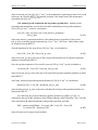
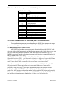
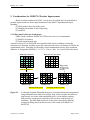
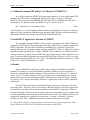
Gross Primary Production (GPP) 1-km MODIS image
Global GPP image created by Andrew Neuschwander.
Version 2.0, December 2, 2003
MOD17 User’s Guide
MODIS Land Team
This page intentionally left blank.
Version 2.0, 12/2/2003
Page 2 of 57
MOD17 User’s Guide
MODIS Land Team
Table of Contents
Synopsis
8
CHAPTER I. THE MODIS ALGORITHM
1. The Algorithm, Background, and Overview
1.1 Estimating vegetative productivity from absorbed radiation
1.2 The Biophysical Variability of ε
1.3 The MOD17A2/MOD17A3 algorithm logic
2. Simplifying Assumptions for Global Applicability
2.1 The BPLUT and constant biome properties
2.2 Leaf area index and fraction of absorbed photosynthetically active radiation
2.3 DAO daily meteorological data
3. Dependence on MODIS Land Cover Classification (MOD12Q1)
4. Practical Considerations for Processing and Use of MODIS Data
4.1 MODIS tile projection characteristics
4.2 File format of MOD17 end products
4.3 Data set characteristics
4.4 Links to MODIS-friendly tools
5. Data Collection History
6. Quality Assurance
6.1 GPP and NPP Quality Assurance Variable Scheme
6.2 Identifying non-terrestrial fill values in the GPP/NPP data products
7. Missing Data
8. Usefulness of Data for Answering Research Questions
9. Considerations for MOD17A2 Product Improvement
9.1 Filling model values for cloudy pixels
9.2 Data compositing
9.3 Land cover
8
8
9
11
16
16
16
18
18
20
20
21
26
26
28
28
30
30
33
33
34
34
35
35
CHAPTER II. PROPOSED IMPROVEMENTS TO THE COLLECTION
4 ALGORITHM
1. Introduction
2. Problems with Collection 4 MOD17
3. Improvements from Collection 4 to Collection 4.5
4. Addition of Annual GPP and QC to Collection 4.5 MOD17A3
5. Final BPLUT applied to Collection 4.5 MOD17
6. Results
37
37
38
42
42
42
CHAPTER III. ORDERING MOD17A2 DATA
1. Naming Conventions
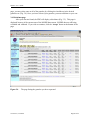
2. Logging into the EDG
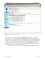
3. Searching the Data
3.1 EDG search page
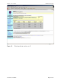
3.2 Search in Progress page
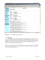
3.3 Granule listing page
3.4 Disclaimer page
43
43
44
44
46
47
48
Version 2.0, 12/2/2003
Page 3 of 57
MOD17 User’s Guide
MODIS Land Team
Table of Contents (cont.)
4. Ordering the Data
4.1 Ordering options page
4.2 Ordering options page (part II)
4.3 Order form
4.4 Reviewing your order (Step 3)
4.5 Submitting the order
5. The DataPool
49
49
49
52
53
53
54
MODIS FAQ’s
REFERENCES
55
56
Version 2.0, 12/2/2003
Page 4 of 57
MOD17 User’s Guide
MODIS Land Team
List of Figures
Fig.
Caption
Page
CHAPTER I.
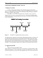
1.1
Flowcharts showing the logic behind the MOD17 Algorithm in calculating both
(a) 8-day average GPP and (b) annual NPP.
1.2
The TMIN and VPD attenuation scalars are simple linear ramp functions of daily
TMIN and VPD.
2.1
The linkages among MODIS land products.
2.2
Comparisons of DAO and observed meteorological data.
4.1
MODIS tiling system. Any location on the earth can be spatially referenced using
the horizontal (H) and vertical (V) designators. Each tile is 1200 x 1200
kilometers.
6.1
A diagram for a hypothetical MOD17A2 quality assurance value of 4.
9.1
A schematic diagram illustrating the process of spatial and temporal interpolation
using information from land cover and QA flags. In this example, the landcover
map has only two values (dark and dashed ones). In the bottom windows, dark
pixels are cloudy pixels, and white pixels are those with the best QA conditions.
The thick-bordered pixels are the pixels selected after filtering. In temporal filling,
data from the previous week is used to fill MOD15 or MOD17A2.
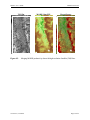
9.5
Merging MODIS productivity data with high-resolution LandSat (TM) Data.
CHAPTER II.
2.1
Comparison of temporal profiles of 2001 Collection 4 MOD15A2 with original
values (FPAR_noQc, LAI_noQc) and temporally linearly-filled FPAR and LAI
(FPAR_filling, LAI_filling), and of temporal profiles of MOD17A2 with original
MOD15A2 inputs (GPP_noQc, PSN_noQc), and MOD17A2 with filled
MOD15A2 (GPP_filling, PSN_filling). The pixel is located in the Amazon
rainforest (lat = -1.0, lon = -60) with the MODIS land cover Evergreen Broadleaf
Forest (EBF).
2.2
Comparison of Collection 4 and Collection 4.5 MOD17A2 GPP (composite period
241) and MOD17A3 NPP for 2001.
3.1
3.2
Distribution of more than 5,000 WMO stations for 2001 and 2002.
Percent of WMO stations with changes in RMSE and COR between spatially
interpolated and non-interpolated DAO. For most stations, DAO accuracies are
improved (reduced RMSE and increased COR) as a result of spatial interpolation.
Version 2.0, 12/2/2003
Page 5 of 57
10
12
16
19
27
30
34
36
39
40
41
41
MOD17 User’s Guide
MODIS Land Team
List of Figures (cont.)
CHAPTER III.
1.1
The MOD17A2 Standard Product naming convention.
2.1
The EDG home page.
3.1
The EDG search page.
3.2
Choosing the time range.
3.3
The “Search in progress” page.
3.4
The page listing the granules you have requested.
3.5
The disclaimer.
4.1
Choosing ordering options.
4.2
Choosing ordering options, part II.
4.3
Choosing ordering options, the “Ready” page.
4.4
The order form.
4.5
Verifying and submitting the order.
Version 2.0, 12/2/2003
43
44
45
46
47
48
49
50
51
52
53
54
Page 6 of 57
MOD17 User’s Guide
MODIS Land Team
List of Tables
Table Title
CHAPTER I.
1.1
BPLUT parameters for daily gross primary productivity.
1.2
BPLUT parameters for daily maintenance respiration.
1.3
BPLUT parameters for annual maintenance and growth respiration.
2.1
The Biome Properties Look-Up Table (BPLUT) for MOD17.
3.1
The land cover types used in the MOD17 Algorithm.
4.1
ECS Metadata Summary for PSN, PSNnet and NPP Data Products.
Page
11
12
14
17
20
22
4.2
6.1
6.2
6.3
6.4
Summary of output variables from the MODIS vegetation productivity
algorithm.
GPP 8-bit Quality Assurance Variable bit-field definitions (Collection 3 and
earlier).
GPP 8-bit Quality Assurance Variable bit-field definitions (Collection 4).
NPP 8-bit Quality Assurance Variable bit-field definitions (Collection 4).
GPP 8-day summation and annual NPP non-terrestrial fill-value code
definitions.
Version 2.0, 12/2/2003
26
31
32
32
33
Page 7 of 57
MOD17 User’s Guide
MODIS Land Team
Synopsis
Vegetative productivity is the source of all food, fiber and fuel available for human
consumption and therefore defines the habitability of the earth. The rate at which light energy is
converted to plant biomass is termed primary productivity. The sum total of the converted
energy is called gross primary productivity (GPP). Net primary productivity (NPP) is the
difference between GPP and energy lost during plant respiration (Campbell 1990).
Global productivity can be estimated by combining remote sensing with carbon cycle
processing. The U.S. National Aeronautics and Space Administration (NASA) Earth Observing
System (EOS) currently “produces a regular global estimate of gross primary productivity (GPP)
and annual net primary productivity (NPP) of the entire terrestrial earth surface at 1-km spatial
resolution, 150 million cells, each having GPP and NPP computed individually” (Running et al.
2000; Thornton et al. 2002). The MOD17A2/A3 User’s Guide provides a description of the
Gross and Net Primary Productivity algorithms (MOD17A2/A3) designed for the MODIS sensor
aboard the Aqua and Terra platforms. The resulting 8-day products are archived at a NASA
DAAC (Distributed Active Archive Center). The document is intended to provide both a broad
overview and sufficient detail to enable the successful use of the data in research and
applications.
CHAPTER I. THE MODIS ALGORITHM
1. The Algorithm, Background and Overview
1.1. Estimating vegetative productivity from absorbed radiation
A conservative relationship between absorbed photosynthetically active radiation
(APAR) and net primary productivity (NPP) was first proposed by Monteith (Monteith 1972;
Monteith 1977). This original logic, known as “radiation use efficiency”, suggested that the NPP
of well-watered and fertilized annual crop plants was linearly related to the amount of absorbed
photosynthetically active solar radiation (APAR). APAR depends upon [1] the geographic and
seasonal variability of daylength and potential incident radiation, as modified by cloudcover and
aerosols, and [2] the amount and geometry of displayed leaf material. Monteith’s logic,
therefore, combines the meteorological constraint of available sunlight at a site with the
ecological constraint of the amount of leaf-area capable of absorbing that solar energy. Such a
combination avoids many of the complexities of carbon balance theory.
The radiation use efficiency logic requires an estimate of APAR, while the more typical
application of remote sensing data is to provide an estimate of the fraction of incident PAR
absorbed by the surface (FPAR). Measurements or estimates of PAR are therefore required in
addition to the remotely sensed FPAR. Fortunately, for studies over small spatial domains with
in situ measurements of PAR at the surface, the derivation of APAR from satellite-derived FPAR
is straightforward (APAR = PAR * FPAR). Implementation of radiation use efficiency for the
MODIS productivity algorithm depends on global daily estimates of PAR, ideally at the same
spatial resolution as the remote sensing inputs, a challenging problem. Currently, large-scale
meteorological data are provided by the NASA Data Assimilation Office (DAO;
http://polar.gsfc.nasa.gov/index.php) (Atlas and Lucchesi 2000) at a resolution of 1° x 1.25°. In
Version 2.0, 12/2/2003
Page 8 of 57
MOD17 User’s Guide
MODIS Land Team
spite of the strong theoretical and empirical relationship between remotely-sensed surface
reflectance and FPAR, accurate estimates of vegetative productivity (GPP, NPP) will depend
strongly on the quality of the radiation inputs.
1.2 The Biophysical Variability of ε
The PAR conversion efficiency ε, varies widely with different vegetation types (Field et
al. 1995, Prince and Goward 1985, Turner et al. 2003). There are two principle sources of this
variability. First, with any vegetation, some photosynthesis is immediately used for maintenance
respiration. For the annual crop plants from the original theory of Monteith (1972), these
respiration costs were minimal, so ε was typically around 2 gC/MJ. Respiration costs, however,
increase with the size of perennial plants. Hunt (1994) found published ε values for woody
vegetation were much lower, from about 0.2 to 1.5 gC/MJ. and hypothesized that this was the
result of respiration from the 6-27% of living cells in the sapwood of woody stems (Waring and
Running 1998).
The second source of variability in ε is attributed to suboptimal climatic conditions. To
extrapolate Monteith’s original theory, designed for well-watered crops only during the growing
season, to perennial plants living year around, certain severe climatic constraints must be
recognized. Evergreen vegetation such as conifer trees or schlerophyllous shrubs absorb PAR
during the non-growing season, yet sub-freezing temperatures stop photosynthesis because leaf
stomata are forced to close (Waring and Running 1998). As a global generalization, we truncate
GPP on days when the minimum temperature is below 0° C. Additionally, high vapor pressure
deficits, > 2000Pa, have been shown to induce stomatal closure in many species. This level of
daily atmospheric water deficit is commonly reached in semi-arid regions of the world for much
of the growing season. So, our algorithm mimics this physiological control by progressively
limiting daily GPP, reducing ε when high vapor pressure deficits are computed from the surface
meteorology. We also assume nutrient constraints on vegetation growth to be quantified by
limiting leaf area, rather than attempting to compute a constraint through ε. This assumption isn’t
entirely accurate, as ranges of leaf nitrogen and photosynthetic capacity occur in all vegetation
types (Reich et al.. 1994, Reich et al 1995, Turner et al 2003). Spectral reflectances are
somewhat sensitive to leaf chemistry, so the MODIS derived FPAR and LAI may represent some
differences in leaf nitrogen content, but in an undetermined way.
To quantify these biome- and climate-induced ranges of ε, we simulated global NPP in
advance with a complex ecosystem model, BIOME-BGC, and computed the ε or conversion
efficiency from APAR to final NPP. This Biome Parameter Look-Up Table (BPLUT) contains
parameters for temperature and VPD limits, specific leaf area and respiration coefficients for
representative vegetation in each biome type (Running et al. 2000, White et al. 2000). The
BPLUT also defines biome differences in carbon storage and turnover rates.
Since the relationships of environmental variables, especially temperature, to the
processes controlling GPP and those controlling autotrophic respiration have fundamentally
different forms (Schwarz et al. 1997; Maier et al. 1998), it seems likely that the empirical
parameterization of the influence of temperature on production efficiency would be more robust
if the gross production and autotrophic respiration processes were separated. This is the
approach employed in the MOD17 algorithm.
Version 2.0, 12/2/2003
Page 9 of 57
MOD17 User’s Guide
MODIS Land Team
GPP
fine root
mass
Figure 1.1.
Flowcharts showing the logic behind the MOD17 Algorithm in calculating both
(a) 8-day average GPP and (b) annual NPP.
Version 2.0, 12/2/2003
Page 10 of 57
MOD17 User’s Guide
Table 1.1.
Parameter
εmax
TMINmax
TMINmin
VPDmax
VPDmin
MODIS Land Team
BPLUT parameters for daily gross primary productivity.
Units
Description
-1
(kg C MJ )
The maximum radiation conversion efficiency
(°C)
The daily minimum temperature at which ε = εmax (for
optimal VPD)
(°C)
The daily minimum temperature at which ε = 0.0 (at any
VPD)
(Pa)
The daylight average vapor pressure deficit at which
ε = εmax (for optimal TMIN)
(Pa)
The daylight average vapor pressure deficit at which
ε = 0.0 (at any TMIN)
1.3. The MOD17A2/MOD17A3 algorithm logic
1.3a. Gross primary productivity. The core science of the algorithm is an application
of the described radiation conversion efficiency concept to predictions of daily GPP, using
satellite-derived FPAR (from MOD15) and independent estimates of PAR and other surface
meteorological fields (from DAO data), and the subsequent estimation of maintenance and
growth respiration terms that are subtracted from GPP to arrive at annual NPP. The maintenance
respiration (MR) and growth respiration (GR) components are derived from allometric
relationships linking daily biomass and annual growth of plant tissues to satellite-derived
estimates of leaf area index (LAI, MOD15). These allometric relationships have been developed
from an extensive
literature review, and incorporate the same parameters as those used in the BIOME-BGC
ecosystem process model (Running and Hunt 1993; White et al. 2000; Thornton et al. 2002).
For any given pixel within the global set of 1-km land pixels, estimates of both GPP and
NPP are calculated. The calculations, summarized in Figure 1.1, are a series of steps, some of
which (e.g., GPP) are calculated daily, and others (e.g., NPP) on an annual basis. Calculations of
daily photosynthesis (GPP) are shown in the lower half of Figure 1.1a. An 8-day estimate of
FPAR from MOD15 and daily estimated PAR from DAO are multiplied to produce daily APAR
for the pixel. Based on the at-launch landcover product (MOD12), a set of biome-specific
radiation use efficiency parameters are extracted from the Biome Properties Look-Up Table
(BPLUT) for each pixel. There are five parameters used to calculate GPP, as shown in Table
1.1. The actual biome-specific values associated with these parameters will be discussed in
Section 3, and the entire BPLUT is shown in Table 2.1.
The two parameters for TMIN and the two parameters for VPD are used to calculate the
scalars that attenuate εmax to produce the final ε (kg C MJ-1) used to predict GPP such that
ε = εmax * TMIN_scalar * VPD_scalar
(1.1)
The attenuation scalars are simple linear ramp functions of daily TMIN and VPD, as illustrated
for TMIN in Figure 1.2. Values of TMIN and VPD are obtained from the DAO dataset, while
the value of εmax is obtained from the BPLUT. The resulting radiation use efficiency coefficient
Version 2.0, 12/2/2003
Page 11 of 57
MODIS Land Team
1.0
1.0
VPD Scalar
TMIN Scalar
MOD17 User’s Guide
0.0
0.0
TMINmin
Figure 1.2.
TMINmax
VPDmin
VPDmax
The TMIN and VPD attenuation scalars are simple linear ramp functions of daily
TMIN and VPD.
Table 1.2.
BPLUT parameters for daily maintenance respiration.
Parameter
Units
Description
2
-1
SLA
(m kg C )
Projected leaf area per unit mass of leaf carbon
froot_leaf_ratio None
Ratio of fine root carbon to leaf carbon
-1
-1
leaf_mr_base
(kg C kg C day ) Maintenance respiration per unit leaf carbon per
day at 20°C
-1
-1
froot_mr_base
(kg C kg C day ) Maintenance respiration per unit fine root carbon
per day at 20°C
Q10_mr
None
Exponent shape parameter controlling respiration
as a function of temperature
ε is combined with estimates of APAR to calculate GPP (kg C day-1) as
GPP = ε * APAR
(1.2)
where APAR = IPAR * FPAR. IPAR (PAR incident on the vegetative surface ) must be
estimated from incident shortwave radiation (SWRad, provided in the DAO dataset) as
IPAR = (SWRad * 0.45)
(1.3)
While GPP (Equation 1.2) is calculated on a daily basis, 8-day summations of GPP are created
and these summations are available to the public. The summations are named for the first day
included in the 8-day period.
~ Each summation consists of 8 consecutive days of data, and there are 46 such summations
created for each calendar year of data collection. To obtain an estimate of daily GPP for this 8day period, it is necessary to divide the value obtained during a data download by eight for the
first 45 values/year and by five (or six in a leap year) for the final period.
1.3b. Daily maintenance respiration and net photosynthesis. Maintenance respiration
costs (MR) for leaves and fine roots, summarized in the lower half of Figure 2.1a, are also
calculated on a daily basis. There are five parameters within the BPLUT (Table 2.2) needed to
Version 2.0, 12/2/2003
Page 12 of 57
MOD17 User’s Guide
MODIS Land Team
calculate daily MR, which is dependent upon leaf or fine root mass, base MR at 20°C, and daily
average temperature. Leaf mass (kg) is calculated as
Leaf_Mass = LAI / SLA
(1.4)
where LAI, the leaf area index (m2 leaf m-2 ground area), is obtained from MOD15 and the
specific leaf area (SLA, projected leaf area kg-1 leaf C) for a given pixel is obtained from the
BPLUT.
Fine root mass (Fine_Root_Mass, kg) is then estimated as
Fine_Root_Mass = Leaf_Mass * froot_leaf_ratio
(1.5)
where froot_leaf_ratio is the ratio of fine root to leaf mass (unitless) as obtained from the
BPLUT.
Leaf maintenance respiration (Leaf_MR, kg C day-1) is calculated as
Leaf_MR = Leaf_Mass * leaf_mr_base * Q10_mr [(Tavg - 20.0) / 10.0]
(1.6)
where leaf_mr_base is the maintenance respiration of leaves (kg C kg C-1 day-1) as obtained from
the BPLUT and Tavg is the average daily temperature (°C) as estimated from the DAO
meteorological data.
The maintenance respiration of the fine root mass (Froot_MR, kg C, day-1) is calculated as
Froot_MR = Fine_Root_Mass * froot_mr_base * Q10_mr [(Tavg - 20.0) / 10.0]
(1.7)
where froot_mr_base is the maintenance respiration per unit of fine roots (kg C kg C-1 day-1) at
20°C as obtained from the BPLUT.
Finally, PSNnet (kg C day-1) can be calculated from GPP (Equation 2.2) and maintenance
respiration (Equations 2.5, 2.6) as
PSNnet = GPP – Leaf_MR - Froot_MR
(1.8)
As with GPP, PSNnet is summed over an 8-day period.
~ This product does not include the maintenance respiration associated with live wood
(Livewood_MR), nor does it include growth respiration (GR).
1.3c. Annual maintenance respiration. Given a calendar year’s worth of outputs from
the daily algorithm, the annual algorithm (Fig. 1.1b) estimates annual NPP by first calculating
live woody tissue maintenance respiration, and then estimating growth respiration costs for
leaves, fine roots, and woody tissue using values defined in Table 1.3. Finally, these components
are subtracted from the accumulated daily PSNnet to produce an estimate of annual NPP.
Version 2.0, 12/2/2003
Page 13 of 57
MOD17 User’s Guide
MODIS Land Team
Table 1.3.
BPLUT parameters for annual maintenance and growth respiration.
Parameter
Units
Description
livewood_leaf_ratio
None
Ratio of live wood carbon to annual
maximum leaf carbon
-1
-1
livewood_mr_base
(kg C kg C day ) Maintenance respiration per unit live
wood carbon per day at 20°C
leaf_longevity
(yrs)
Average leaf lifespan
leaf_gr_base
(kg C kg C-1)
Respiration cost to grow a unit of leaf
carbon
froot_leaf_gr_ratio
None
Ratio of live wood to leaf annual growth
respiration
livewood_leaf_gr_ratio
None
Ratio of live wood to leaf annual growth
respiration
deadwood_leaf_gr_ratio
None
Ratio of dead wood to leaf annual growth
respiration
ann_turnover_proportion
None
Annual proportion of leaf turnover
Annual maximum leaf mass, the maximum value of daily leaf mass, is the primary input
for both live wood maintenance respiration (Livewood_MR) and whole-plant growth respiration
(GR). To account for Livewood_MR, it is assumed that the amount of live woody tissue is (1)
constant throughout the year and (2) related to annual maximum leaf mass. Once the live woody
tissue mass has been determined, it can be used to estimate total annual livewood maintenance
respiration. This approach relies on empirical studies relating the annual growth of leaves to the
annual growth of other plant tissues. The compilation study by Cannell (1982) is an excellent
resource, providing the basis for many of the relationships developed for this portion of the
MOD17 Algorithm and tested with the BIOME-BGC ecosystem process model. Leaf longevity
is required to estimate annual leaf growth for evergreen forests, but it is assumed to be less than
one year for deciduous forests, which replace all foliage annually. This logic further assumes
that there is no litterfall in deciduous forests until after maximum annual leaf mass has been
attained. The parameters relating annual leaf growth respiration costs to annual fine root, live
wood, and dead wood growth respiration were calculated directly from similar parameters
developed for the BIOME-BGC model (White et al. 2000; Thornton et al. 2002).
To create the annual NPP term, the MOD17 algorithm maintains a series of daily pixelwise terms to appropriately account for plant and soil respiration. To determine livewood
maintenance respiration, the mass of livewood (Livewood_Mass, kg C) is calculated as
Livewood_Mass = ann_leaf_mass_max * livewood_leaf_ratio
(1.9)
where ann_leaf_mass_max is the annual maximum leaf mass for a given pixel (kg C) obtained
from the daily Leaf_Mass calculation (Equation 1.4). The livewood_leaf_ratio is the ratio of live
wood mass to leaf mass (unitless), and is obtained from the BPLUT. Once the mass of live wood
has been determined, it is possible to calculate the associated maintenance respiration
(Livewood_MR, kg C day-1) as
Livewood_MR = Livewood_Mass * livewood_mr_base * annsum_mrindex
Version 2.0, 12/2/2003
(1.10)
Page 14 of 57
MOD17 User’s Guide
MODIS Land Team
where livewood_mr_base (kg C kg C-1 day-1) is the maintenance respiration per unit of live wood
carbon per day from the BPLUT and annsum_mrindex is the annual sum of the maintenance
respiration term Q10_mr [(Tavg-20.0)/10.0].
1.3d. Annual growth respiration and net primary productivity. Annual growth
respiration and maintenance costs are based on their relationship to leaf growth respiration
(Leaf_GR, kg C day-1), which is calculated as
Leaf_GR = ann_leaf_mass_max * ann_turnover_proportion *
leaf_gr_base
(1.11)
where ann_turnover_proportion (unitless) is the annual turnover proportion of leaves and
leaf_gr_base is the base growth respiration (kg C kg C-1 day-1) for leaves. Both of these terms
are acquired from the BPLUT.
Growth respiration for fine roots (Froot_GR, kg C day-1) is calculated as
Froot_GR = Leaf_GR * froot_leaf_gr_ratio
(1.12)
where froot_leaf_gr_ratio is the ratio of fine root growth respiration to leaf growth respiration
(unitless) as found in the BPLUT.
Next, the growth respiration of livewood (Livewood_GR, kg C day-1) can be calculated as
Livewood_GR = Leaf_GR * livewood_leaf_gr_ratio
(1.13)
where livewood_leaf_gr_ratio is the ratio of livewood leaf growth respiration (unitless) as found
in the BPLUT.
And, lastly, deadwood growth respiration (Deadwood_GR, kg C day-1) is calculated as
Deadwood_GR = Leaf_GR * deadwood_leaf_gr_ratio
(1.14)
where deadwood_leaf_gr_ratio is the ratio of deadwood to leaf growth respiration (unitless) as
found in the BPLUT.
As a final step, the per-pixel annual net primary productivity (NPP, kg C day-1) is
calculated as the sum of the cumulative daily PSNnet (annsum_daily PSNnet kg C day-1) less the
costs associated with annual maintenance and growth respiration, such that
NPP = annsum_dailyPSNnet – Livewood_MR – Leaf_GR – Froot_GR –
Livewood_GR – Deadwood_GR
(1.15)
where all terms have been previously defined.
Version 2.0, 12/2/2003
Page 15 of 57
MOD17 User’s Guide
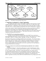
1 km MODIS
Surface
Reflectances
MOD09
Land
Cover/Biome
Designation
MOD12
MODIS Land Team
MODIS product suite
1 km MODIS
Surface
Reflectances
MODAGAGG
LAI, FPAR
Daily Intermediate
MOD15A1
Figure 2.1.
LAI, FPAR
8-day summation
MOD15A2
GPP, PSNnet
8-day summation
MOD17A2
GPP, PSNnet
Daily intermediate
MOD17A1
Annual
NPP
MOD17A3
The linkages among MODIS land products.
2. Simplifying Assumptions for Global Applicability
In an ideal world, remote sensing would render an infallibly accurate depiction of surface
conditions and deliver the data in a timely, cost-effective manner for every square meter of the
earth’s land surface. Unfortunately, such a system does not exist, and even if it did, it would be
impossible to derive vegetation productivity algorithms suited for all combinations of vegetation
at such a fine resolution. NASA’s Earth Observing System, and more specifically, the MODIS
instrument have been tasked with documenting and monitoring global biospheric health
(Running et al. 2000; Thornton et al. 2002). Among other things, such a task requires timely and
objective measures of vegetation productivity. This requisite necessitates several noteworthy
simplifying assumptions discussed below.
2.1. The BPLUT and constant biome properties
Arguably, the most significant assumption made in the MOD17 logic is that biomespecific physiological parameters do not vary with space or time. These parameters are outlined
in the BPLUT (Table 2.1) within the MOD17 algorithm. The BPLUT constitutes the
physiological framework for controlling simulated carbon sequestration. These biome-specific
properties are not differentiated for different expressions of a given biome, nor are they varied at
any time during the year. In other words, a semi-desert grassland in Mongolia is treated the
same as a tallgrass prairie in the Midwestern United States. Likewise, a sparsely vegetated
boreal evergreen needleleaf forest in Canada is functionally equivalent to its coastal temperate
evergreen needleleaf forest counterpart.
2.2. Leaf area index (LAI) and fraction of absorbed photosynthetically active radiation
(FPAR)
As illustrated in Figure 2.1, the primary productivity at a pixel is dependent upon, among
other things, LAI and FPAR, calculated with the MOD15 algorithm. The LAI/FPAR product is
an 8-day composite product. The MOD15 compositing algorithm uses a simple selection
rule whereby the maximum FPAR (across the eight days) is chosen for the inclusion as the
output pixel. The same day chosen to represent the FPAR measure also contributes the current
pixel’s LAI value. This means that although primary productivity is calculated daily, the
MOD17 algorithm necessarily assumes that leaf area and FPAR do not vary during a given 8-day
Version 2.0, 12/2/2003
Page 16 of 57
MOD17 User’s Guide
Table 2.1.
MODIS Land Team
The Biome Properties Look-Up Table (BPLUT) for MOD17.
Version 2.0, 12/2/2003
Page 17 of 57
MOD17 User’s Guide
MODIS Land Team
period. Compositing of LAI and FPAR is required to provide an accurate depiction of global
leaf area dynamics with consideration of spectral cloud contamination, particularly in the tropics.
2.3. DAO daily meteorological data
The MOD17 algorithm computes productivity at a daily time step. This is made possible
by the daily meteorological data, including average and minimum air temperature,
incident PAR and specific humidity, provided by the Data Assimilation Office (DAO), a branch
of NASA (Schubert et al. 1993). These data, produced every six hours, are derived using a
global circulation model (GCM), which incorporates both ground and satellite-based
observations. These data are distributed at a resolution of 1° by 1.25° (originally 1° x 1°) in
contrast to the 1-km gridded MOD17 outputs. It is assumed that the coarse resolution
meteorological data provide an accurate depiction of ground conditions and are homogeneous
within the spatial extent of each cell. Preliminary studies done by Numerical Terradynamic
Simulation Group (NTSG) suggest that the relationship between surface observations and DAO
data across the U.S. appears reasonable (Fig. 2.2), but comparisons have yet to be made on a
global scale.
3. Dependence on MODIS Land Cover Classification (MOD12Q1)
One of the first MODIS products used in the MOD17 algorithm is the Land Cover
Product, MOD12Q1. The importance of this product cannot be overstated as the MOD17
algorithm relies heavily on land cover type through use of the BPLUT (Table 3.1). While, the
primary product created by MOD12 is a 17-class IGBP (International Geosphere-Biosphere
Programme) landcover classification map (Belward et al. 1999; Scepan 1999), the MOD17
algorithm employs Boston University’s UMD classification scheme (Table 3.1). More details on
these and other schemes and their quality control considerations can be found at the Land Cover
Product Team website (http://geography.bu.edu/landcover/userguidelc/index.html).
Given the global nature and daily time-step of the MODIS project, a broad classification
scheme, which retains the essence of land cover, is necessary. Since all MODIS products are
designed at a 1-km grid scale, it can be difficult to obtain accurate land cover in areas with
complex vegetation, and misclassification can occur. However, studies have suggested that the
MODIS vegetation maps are accurate to within 65-80%, with higher accuracies for pixels that
are largely homogeneous, and allow for consistent monitoring of the global land cover (Hansen
et al. 2000).
Version 2.0, 12/2/2003
Page 18 of 57
MOD17 User’s Guide
MODIS Land Team
30
35
Average Temperature from the DAO (deg C)
Minimum Temperature from the DAO (deg C)
25
20
15
10
Arizona
California
North Carolina
North Dakota
5
0
0
5
10
15
20
25
30
25
20
15
10
10
30
Arizona
California
North Carolina
North Dakota
15
Observed Minimum Temperature (deg C)
25
30
35
35
Daily Total Shortwave Radiation from the DAO (MJ m-2 d-1)
4000
Average Daytime VPD from the DAO (Pa)
20
Observed Average Temperature (deg C)
3000
2000
1000
Arizona
California
North Carolina
North Dakota
0
0
1000
2000
3000
Observed Average Daytime VPD (Pa)
Figure 2.2.
4000
30
25
20
15
Arizona
California
North Carolina
North Dakota
10
10
15
20
25
30
35
Observed Daily Total Shortwave Radiation (MJ m-2 d-1)
Comparisons of DAO and observed meteorological data.
Version 2.0, 12/2/2003
Page 19 of 57
MOD17 User’s Guide
Table 3.1.
MODIS Land Team
The land cover types used in the MOD17 Algorithm.
UMD Land Cover Types
Class Value Class Description
0
Water
1
Evergreen Needleleaf Forest
2
Evergreen Broadleaf Forest
3
Deciduous Needleleaf Forest
4
Deciduous Broadleaf Forest
5
Mixed Forest
6
Closed Shrubland
7
Open Shrubland
8
Woody Savanna
9
Savanna
10
Grassland
12
Cropland
13
Urban or Built-Up
16
Barren or Sparsely Vegetated
254
Unclassified
255
Missing Data
4. Practical Considerations for Processing and Use of MODIS Data
Two considerations paramount to understanding the MODIS data stream are the unique
projection and tiling system and the file format inherent to all MODIS land products.
4.1. MODIS tile projection characteristics
All MODIS land products are projected on the Integerized Sinusoidal (ISIN) 10° grid,
where the globe is tiled for production and distribution purposes with 36 tiles along the east-west
axis, and 18 tiles along the north-south axis, each about 1200x1200 kilometers (Fig. 4.1).
MODIS is meeting the stated geolocation requirement of 0.1 pixels at 2 standard deviations for
the 1 km bands (Wolfe, et al. 2002)
~ The Collection 4 projection is Sinusoidal (SIN), while Collections 1-3 use a Integerized
Sinusoidal Projection (ISIN). At a 1 km spatial resolution, the difference between the SIN and
ISIN projections is negligible. The decision to switch from the ISIN to the SIN projection was
made to make the data more compatible with current image processing software.
For many applications it may be convenient to reproject MODIS data from the ISIN or
SIN projection to a different projection that is more suited to the area of interest. Few
proprietary image processing or geographic information system (GIS) software have the
capability to reproject MODIS data from an ISIN projection. Fortunately, however, there are
good tools, which are simple to download and are freely available. The primary tool currently
used to reproject MODIS data in both formats is the MODIS Reprojection Tool (MRT). This
tool, and more information can be found at http://edcdaac.usgs.gov/tools/modis.
Version 2.0, 12/2/2003
Page 20 of 57
MOD17 User’s Guide
MODIS Land Team
4.2. File format of MOD17 end products
All NASA biophysical products are archived in the NASA HDF-EOS data format. HDFEOS is based upon the Hierarchical Data Format pioneered by the National Center for
Supercomputer Applications (NCSA) at the University of Illinois, Champaign/Urbana. The
HDF-EOS format has the advantage of multiple layers of data and supporting ancillary
information (such as projection characteristics, scaling factor, time and date of production etc.) in
a single file. The drawback is that in order to use the actual vegetation productivity layer, one
must extract this layer from the data “stack”. Therefore, the MRT serves two purposes:
[1] reproject MODIS data from ISIN or SIN
[2] extract the desired data layer from the “stack”
Several tools and software systems allow the user to browse through the various data layers
within a given HDF-EOS file. The growing body of HDF-EOS tools can be found at
http://hdfeos.gsfc.nasa.gov/hdfeos/index.html. In addition, the Earth Observing System (EOS)
Core System (ECS) Project Office developed the HDF-EOS to GeoTIFF (HEG).
The HDF-EOS to GeoTIFF (HEG) tool provides conversion for HDF-EOS formatted files
(granules), converting HDF-EOS swath and grid data to HDF-EOS Grid, GeoTIFF, or a generic
binary format. The tool can be used to re-project data from its original format to other standard
projections, as well as to subset data and to mosaic adjacent granules together. The HEG
packages are available for Sun and SGI systems in 'tar' format, and a User's Guide in Microsoft
Word is available. Download and installation instructions can be found at
http://eosweb.larc.nasa.gov/PRODOCS/misr/geotiff_tool.html.
~ Remember, potential byte-order problems can be avoided by unpacking the HDF files (via
the MRT or other means) on the same computer with which they will be doing their analysis.
4.2a. Local (Science Dataset SDS) Attributes. A complete, updated description of each
MODIS land product is found in the MODIS File Specification documents for MOD17A1,
MOD17A2, and MOD17A3 (ftp://modular.gsfc.nasa.gov/pub/LatestFilespecs/). With each SDS
or HDF-EOS gridfield, a series of local SDS attributes are included:
[1] Scale factor and offset (if appropriate)
[2] Data range {minimum,maximum}
[3] Fill value
[4] Longname
4.2b. Global Attributes. All EOS Core System (ECS) data products are assigned a
unique Earth Science Data Type (ESDT), and are provided to users with several types of quality
metadata. Level 3 and 4 data products are gridded using the Integerized Sinusoidal (ISINUS) or
Sinusoidal (SIN) rectangular map projection, and supplied to users with several types of
metadata. Two broad types of metadata are defined, collection level, and granule level, with the
granule level metadata specific to a given granule or tile. All ECS metadata entries are formally
introduced to the system and are registered within the ESDT definition. For complete details on
ECS metadata issues, interested readers are encouraged to visit URL
http://observer.gsfc.nasa.gov/. A fairly complete ECS related glossary relevant to metadata may
be found at: http://ecsinfo.gsfc.nasa.gov/sec2/glossary.html.
Version 2.0, 12/2/2003
Page 21 of 57
MOD17 User’s Guide
MODIS Land Team
At the tile (or granule) level, the standard ECS metadata are organized into three different
sections, each appearing in a given HDF-EOS file as a global character attribute (Table 4.1). A
granule is the smallest unit of data that is produced, inventoried, and archived within the
EOSDIS. Within each of these large metadata blocks, data are organized using the Object Data
Language (ODL) conventions established by NASA, with the data itself formatted as a series of
name-value pairs or Parameter Value Language (PVL). An example of PVL syntax is the
“GROUP… END_GROUP” and OBJECT… END_OBJECT” form commonly found in both the
MCF files and each granule or tile HDF-EOS file. ODL enables the internal software used in
MODIS production to access data defined within the Metadata Control File (MCF), with a
unique MCF file defined for each ESDT that is archived, such as MOD17A2, or MOD17A3.
Users interested in quickly viewing the metadata contents of a HDF-EOS file may wish
to use the commonly available HDF utility called ncdump. The ncdump utility for most
computer platforms may be obtained from the National Center for Supercomputer Applications
(NCSA) HDF web site (http://hdf.ncsa.uiuc.edu/hdftools.html) as well as from common NASA
HDF-EOS tool URL sites. To produce a listing at the console of Science Data Set (SDS)
properties as well as ECS metadata, enter a command such as:
“ncdump –h MOD17A2.A2002353.h08v05.003.2003008095623.hdf”
Other interactive (graphical user interface based) software tools users may employ to
view the original ECS metadata information in a HDF-EOS tile are HDFLook on Unix/Linux,
and the Java-based WebWinds tool available on most platforms. Additional information on
these tools can be found in Section 4.4.
Principal Investigators who wish to define additional attributes specific to their data
product may also use the Product Specific Attribute (PSA) mechanism, wherein a limited
number of attributes not covered in the standard metadata may be included in a granule. Note
that the size of a global file attribute in HDF v4.x (and therefore, in an HDF-EOS file) is limited
to 64Kb. The ECS tile level metadata sections are summarized in Table 4.1. Note that although
the examples below refer to the MOD17A2 (8-day photosynthesis) ESDT, these metadata also
apply to the MOD17A3 annual NPP product.
4.2b.i. Core and Archive Metadata: What’s The Difference? The ECS Core metadata
(CoreMetadata.0) are granule level metadata that describe a number of useful tile level attributes
for the granules held in a common Collection, such as the current Collection 4. These metadata
are also known as INVENTORY metadata, reflecting the fact they constitute a baseline resource
Table 4.1. ECS Metadata Summary for PSN, PSNnet and NPP Data Products.
Block
Organization
Contents
StructMetadata.0
Object Data Language (ODL) Geospatial data, tile origin
coordinates, map projection
attributes
CoreMetadata.0
Object Data Language (ODL) Inventory attributes
ArchiveMetadata.0 Object Data Language (ODL) Archive metadata attributes
Version 2.0, 12/2/2003
Page 22 of 57
MOD17 User’s Guide
MODIS Land Team
describing the inventory of data available. INVENTORY (or Core) metadata includes all
granule-level metadata that will reside in ECS inventory tables and will thus be searchable.
Archive metadata (stored in each granule in the ArchiveMetadata.0 block), on the other
hand, contain metadata fields that the producer wants to accompany the granule when it is
delivered to end-users, but need not be searchable by the system. Both the Core and Archive
metadata elements are defined in the Metadata Control File (MCF) that accompany each processgeneration executable (PGE) in the system.
4.2b.ii. StructMetadata Attributes. For gridded Level 3/4 products such as the PSN,
NPP products, a GridStructure object is defined – no swatch structure is defined. The
StructMetadata.0 block contains the physical (e.g. non-science) attributes of the dataset. These
are the minimum attributes that a software reader utility would need to correctly read and
interpret the data at a physical level These include the grid name (MOD_Grid_MOD17A2), the
data set dimensions (1200x1200), the grid upper left origin coordinates, the General
Cartographic Transform Package (GCTP) map projection conversion parameters, and a list of the
science data set (SDS) names.
An abbreviated list of StructMetadata attributes is:
GridName MOD_Grid_MOD17A2
XDim1200 YDim1200
UpperLeftPointMtrs(-8895604.158132,5559752.598833)
LowerRightMtrs(-7783653.638366,4447802.079066)
ProjectionGCTP_ISINUS
ProjParams (6371007.181000,0,0,0,0,0,0,0,86400,0,1,0,0)
SphereCode -1
PixelRegistration HDFE_CENTER
DimensionName YDim Size 1200
DimensionName XDim Size 1200
DataFieldName Gpp_1km
DataType DFNT_INT16
DimList YDim,XDim
DataFieldName PsnNet_1km
DataType DFNT_INT16
DimList YDim,XDim
DataFieldName Psn_QC_1km
DataType DFNT_UINT8
DimList YDim,XDim
ECS MODIS data are generally produced and organized at a high level in terms of
collections. A collection may be considered a generation of data, sharing the common property
of having been produced with a latest “milestone” set of processing algorithms. Within a given
collection, considerable effort is made to re-process all ESDT (products), usually for entire
period when raw Level 0/1A satellite data are available (the period of record), into consistent
structured collections. Since Terra launched in December 1999, there have currently been four
(4) collections produced (Collection 4 is currently being re-processed as of March, 2003), with
each collection taking into account the latest algorithm improvements. Each subsequent
collection is therefore expected to represent incrementally higher quality science data than the
previous. Scientists using Terra MODIS data are therefore encouraged to base their science
research and applications on the most recent collection of data available. Recall that the
Version 2.0, 12/2/2003
Page 23 of 57
MOD17 User’s Guide
MODIS Land Team
collection identifier is also contained in each production tile (individual files) name, as in the
following example tile name shown for MOD13A2 where the collection identifier, “003” is
shown highlighted:
MOD13A2.A2002353.h08v05.003.2003008095623.hdf
A simplified list of CoreMetadata.0 attributes (for the MOD17A2 ESDT) are shown
below. The names are typically self descriptive. Note that Product Specific Attributes (PSA), if
supplied by the Principle Investigator, are contained within the ADDITIONALATTRIBUTE
objects. The spatial extent of the tile is described by the GRINGPOINT (latitude and longitude)
attributes, where these describe the four corner coordinates (N,E,S,W) of the tile.
ADDITIONALATTRIBUTENAME
ADDITIONALATTRIBUTESCONTAINER
ASSOCIATEDINSTRUMENTSHORTNAME
ASSOCIATEDPLATFORMINSTRUMENTSENSORCONTAINER
ASSOCIATEDPLATFORMSHORTNAME
ASSOCIATEDSENSORSHORTNAME
AUTOMATICQUALITYFLAG
AUTOMATICQUALITYFLAGEXPLANATION
DAYNIGHTFLAG
EXCLUSIONGRINGFLAG
GPOLYGONCONTAINER
GRINGPOINTLATITUDE
GRINGPOINTLONGITUDE
GRINGPOINTSEQUENCENO
INPUTPOINTER
LOCALGRANULEID
LOCALVERSIONID
MEASUREDPARAMETERCONTAINER
PARAMETERNAME
PARAMETERVALUE
PGEVERSION
PRODUCTIONDATETIME
QAPERCENTCLOUDCOVER
QAPERCENTINTERPOLATEDDATA
QAPERCENTMISSINGDATA
QAPERCENTOUTOFBOUNDSDATA
RANGEBEGINNINGDATE
RANGEBEGINNINGTIME
RANGEENDINGDATE
RANGEENDINGTIME
REPROCESSINGACTUAL
REPROCESSINGPLANNED
SCIENCEQUALITYFLAG
SCIENCEQUALITYFLAGEXPLANATION
SHORTNAME
VERSIONID
Users may find the following distinction helpful to understand the difference between the
GRINGPOINT coordinates in the CoreMetadata.0 and the NORTH, SOUTH, EAST, WEST
BOUND coordinates in the ArchiveMetadata.0 block. In the ArchiveMetadata block, the
Version 2.0, 12/2/2003
Page 24 of 57
MOD17 User’s Guide
MODIS Land Team
NORTH, SOUTH, EAST, and WEST BOUND coordinates represent a minimum bounding
rectangle (MBR) defined by the tile, rather than the typically trapezoidal shaped polygon
represented by the GRINGPOINT coordinates.
4.2b.iii. ArchiveMetadata Attributes. The following Archive metadata attributes are
designed to assist end-users in using and effectively interpreting the Terra MODIS (PSN, NPP)
data. These attributes are not considered essential as “searchable” metadata in the overall ECS
metadata, partially because some of this information is overlapped by almost equivalent elements
in the CoreMetadata.0 attributes (which as INVENTORY metadata, are searchable).
ALGORITHMPACKAGEACCEPTANCEDATE
ALGORITHMPACKAGEMATURITYCODE
ALGORITHMPACKAGENAME
ALGORITHMPACKAGEVERSION
CHARACTERISTICBINANGULARSIZE
CHARACTERISTICBINSIZE
DATACOLUMNS
DATAROWS
DESCRREVISION
GEOANYABNORMAL
GEOESTMAXRMSERROR
GLOBALGRIDCOLUMNS
GLOBALGRIDROWS
GRANULEBEGINNINGDATETIME
GRANULEDAYNIGHTFLAG
GRANULEENDINGDATETIME
INSTRUMENTNAME
LOCALINPUTGRANULEID
LONGNAME
MAXIMUMOBSERVATIONS
NADIRDATARESOLUTION
NUMBEROFGRANULES
PLATFORMSHORTNAME
PROCESSINGCENTER
PROCESSINGDATETIME
PROCESSINGENVIRONMENT
SPSOPARAMETERS
NORTHBOUNDINGCOORDINATE
EASTBOUNDINGCOORDINATE
SOUTHBOUNDINGCOORDINATE
WESTBOUNDINGCOORDINATE
4.2b.iv. Other Helpful ECS Metadata References. A number of detailed ECS related
web pages and Adobe Postscript documents may be found at http://observer.gsfc.nasa.gov/,
including the document “ECS_ProvidersGuideToMetadata.pdf”. Although document describes
the Terra MODIS metadata scheme from a “providers” standpoint, it is quite useful for interested
readers who want more in-depth coverage on this topic.
Version 2.0, 12/2/2003
Page 25 of 57
MOD17 User’s Guide
MODIS Land Team
4.3. Data set characteristics
As indicated in Figure 1.1 and Table 4.2, the MODIS vegetation productivity data stream
consists of three biophysical products:
[1] 8-day summation GPP
[2] 8-day summation PSNnet
[3] annual NPP
MOD17A2 (Equation 1.2)
MOD17A2 (Equation 1.8)
MOD17A3 (Equation 1.15).
To properly visualize and interpret any of these products, it is necessary to convert them from
scaled digital images to a biophysical quantity. This can be accomplished using the equation:
Biophysical_pixel = scale_factor * digital_value.
(4.1)
where Biophysical_pixel is sequestered carbon (kg C m-2), scale_factor is the gain for the
MODIS productivity products, and digital_value is the numeric value of a file pixel. For
example, if we obtain a mid-summer digital_value of 421 for Gpp_1km from an HDF file, an 8day summation of Gpp_1km would be
Biophysical_pixel = scale_factor * digital_value = 0.0001 * 421 = 0.0421 kg C m-2.
In order to obtain a daily estimate of Gpp_1km, we must divide this number by 8, so that we get
0.0421 kg C m-2 / 8 = 0.00526 kg C m-2 d-1.
The information contained in Table 4.2 can also be found within an HDF-EOS data set and can
be viewed using the various tools found at http://hdfeos.gsfc.nasa.gov/hdfeos/index.html.
~ Remember, the result is an 8-day summation. In order to obtain daily estimates of Gpp_1km
or PsnNet_1km, it is necessary to divide your Biophysical_ pixel value by 8.
4.4. Links to MODIS-friendly tools.
4.4a. HDFLook: HDF and HDF-EOS viewer. This product is available for Solaris,
Alpha VMS, HP-UX, IRIX, AIX, and Linux. It is a handy little tool available at:
http://www-loa.univ-lille1.fr/Hdflook/.
Table 4.2.
Summary of output variables from the MODIS vegetation productivity algorithm.
Summary of MOD17 output variables
Variable
Data
Units
Fill
Scale
Valid Range
Product
Type
Value
Factor
Gpp_1km
Int16
Kg C m-2
32766
0.0001
0 - 30000
MOD17A2
PsnNet_1km
Int16
Kg C m-2
32766
0.0001
-30000 - 30000
MOD17A2
-2
Npp_1km
Int16
Kg C m
32766
0.0001
-30000 - 30000
MOD17A3
Psn_QC_1km
Uint8
N/A
255
N/A
0 - 254
MOD17A2
Npp_QC _1km
Uint8
N/A
255
N/A
0 - 254
MOD17A3
Version 2.0, 12/2/2003
Page 26 of 57
MOD17 User’s Guide
MODIS Land Team
H
0
1 2
3
4
5
6
7
8
9
10 11 12 13 14 15 16 17 18 19 20 21 22 23 24 25 26 27 28 29 30 31 32 33 34 35
0
1
2
3
4
5
6
7
8
V9
10
11
12
13
14
15
16
17
Figure 4.1.
MODIS tiling system. Any location on the earth can be spatially referenced
using the horizontal (H) and vertical (V) designators. Each tile is 1200 x 1200
kilometers.
4.4b. Msphinx: This free utility can read HDF and HDFEOS, and it has some
visualization and other capabilities. Supported platforms include; HP, DEC, Silicon Graphics,
IBM, Sun, and Linux. For more information, go to:
http://www-loa.univ-lille1.fr/Msphinx/.
4.4c. Webwinds: Webwinds is written in Java, enabling it to run on any platform that
supports Java. It is a science data visualization system, capable of reading several data formats.
For more information please see the Webwinds home page at:
http://www.openchannelsoftware.com/projects/WebWinds.
4.4d. LDOPE Tools: LDOPE tools were created to assist in quality assessment of
MODIS Land products. Look at the overview of this toolset at:
http://edcdaac.usgs.gov/tools/ldope.
There are several additional tools available, some free and others not, which support the
HDF-EOS data format in which MODIS data are stored. For a larger listing, see the N.C.S.A.'s
(National Center for Super Computing Applications) tool page at
http://hdf.ncsa.uiuc.edu/tools.html#util.
Version 2.0, 12/2/2003
Page 27 of 57
MOD17 User’s Guide
MODIS Land Team
5. Data Collection History
As with any new product, there have been modifications and improvements to the
MODIS algorithm and outputs. In fact, there have been three such collections (Collections 2, 3
and 4) that may currently be in use. It is important for the user to know which collection they
have, and, furthermore, what assumptions were made in the calculation of that collection. It is
also wise to periodically check the EDC website for any updates on the data. The MOD17
product, at the end of the processing line because of its reliance on other MODIS products (Fig.
2.1), is one of the last products to be updated.
Collection 3. If your data were downloaded prior to December 13, 2002, the
algorithm uses Collection 3 inputs of Land Cover and LAI/FPAR, and an older, less restrictive
BPLUT (To avoid potential confusion, this version of the BPLUT will not appear in the User’s
Guide). The dataset using the older BPLUT is no longer available from the EDC.
If your data were downloaded after December 13, 2002 and before January 15,
2003, then you have the most complete version of Collection 3 data. The primary modification
is a change in the VPD constraints on εmax in Equation 1.1. This product continues to rely upon
Collection 3 inputs of Land Cover (MOD12Q1) and LAI/FPAR (MOD15A2).
Collection 4. Distribution of Collection 4 data began on January 15, 2003. Collection 4
will continue to use the improved algorithm of Collection 3, but will employ Collection 4 inputs
from both the Land Cover and LAI/FPAR algorithms, providing the most up-to-date calculations
available.
Collection 4.5. While not available through the EOS Data Gateway as a standard
product, Collection 4.5 represents an improved MOD17A2/A3 dataset. This dataset includes a
revised BPLUT (Table 3.1) based on the most current research, and is described in Chapter II of
this document. This dataset includes temporal interpolation of cloud-contaminated MOD15A2
LAI/FPAR data and spatial smoothing of the DAO meteorology. This dataset is available upon
request from NTSG (http://www.ntsg.umt.edu). It can be differentiated from the standard
product by looking at the “Product version number” (Figure 1.1, Chapter 3). The standard
product version number will always begin with a “0” (e.g., 004 for Collection 4) as in
MOD17A2.A2003177.h10v04.004.2003201102319.hdf
, while any product created at NTSG will begin with a “1” (e.g., 105 for Collection 4.5) as in
MOD17A2.A2003177.h10v04.105.2003201102319.hdf.
For further information about Collection 4.5, including naming conventions, granules, imagery,
and analysis please visit http://images.ntsg.umt.edu.
~ Users are strongly encouraged to obtain and use Collection 4.5 of the MOD17A2/A3
datasets when available.
6. Quality Assurance
Quality assurance (QA) measures are produced at both the file (e.g. 10-deg tile level) and
at the pixel level. At the tile level, these appear as a set of EOSDIS core system (ECS) metadata
fields, described later in this document. At the pixel level, quality assurance information is
represented by a separate data layer in the HDFEOS file, whose pixel values correspond to
specific quality scoring schemes that vary by product Earth Science Data Type (ESDT). The QC
organization of MOD17A2 and MOD17A3 files generated from Collection 4 and higher is
Version 2.0, 12/2/2003
Page 28 of 57
MOD17 User’s Guide
MODIS Land Team
summarized in Tables 6.1 and 6.2. Significant changes include the new 3-bit scheme of the SCF
bits in MOD17A2, and overall change in the QC of the MOD17A3.
In general, two broad types of quality assurance activities are performed at the SCF and
by the Land Data Operations Processing Environment (LDOPE ) group at Goddard Space
Flight Center:
[1] ?routine QA
[2] ?problem-triggered QA
The primary quality assurance activity routinely conducted at the SCF is the post-processing
assignment of the tile level SCIENCEQUALITYFLAG and accompanying
SCIENCEQUALITYFLAGEXPLANATION. Due to the volume of data, this activity is
performed on only a small percentage of product tiles. Valid components for this field include:
[1] PASSED
[2] FAILED
[3] SUSPECT, BEING INVESTIGATED
[4] NOT BEING INVESTIGATED
Routine QA involves periodic sampling of the product tiles using visual and statistical methods.
Problem triggered QA follows from a report of an inconsistency or other problem in the data,
which has been discovered by the Land Data Operational Product Evaluation (LDOPE) front line
QA personnel, the SCF staff, or users. In this case, an effort is usually made to duplicate the
problem under controlled conditions to resolve it.
During the design phase, the MODIS team chose to provide a Quality Assurance measure
for each pixel. The quality assurance “flags” make it possible for the user to match data sets to
their applications. The user is encouraged to make use of the quality assurance
information associated with each pixel because it permits quick, objective, and repeatable
screening to filter out undesirable pixels. The QA flags that users will find in the MOD17A2
products are summarized in Table 6.1. Each flag is divided into a series of bitfields which can be
parsed to allow separate interpretation of each field for maximum control over the data set. The
EDC DAAC (Earth Resources Observation Systems Data Center Distributed Active Archive
Center) is currently working on tools that will enable the user to automatically parse and process
each bitfield. The process of parsing bitfields may seem confusing at first. As a general rule, if
the user does not wish to examine every bitfield independently, a threshold value of zero should
produce the best quality pixels for scientific analysis, although this may reduce the number of
pixels available for evaluation (Fig. 6.1). There are two steps to interpreting MOD17A2 QA
values:
[1] Convert the file pixel QA number to its binary equivalent.
[2] Alter the binary equivalent to become 8 digits long.
For example, if the binary equivalent is 100, you must add zeroes to the left-hand
side until there are a total of 8 binary digits, since the MOD17A2 QA value is an
8-bit unsigned integer. So, 100 becomes 00000100.
[3] Parse individual bit fields from the 8-bit integer (Figure 6.1) and interpret their
meaning per Table 6.1. Therefore, in this example, the third bit = 1, indicating
that dead detectors caused >50% adjacent detector retrieval.
For example, QA = 4 has a binary equivalent = 100.
Version 2.0, 12/2/2003
Page 29 of 57
MOD17 User’s Guide
MODIS Land Team
4
=
00000100
Leftmost bit 8
00 Significant
clouds NOT present
(clear)
01 Significant
clouds WERE
present
10 Mixed cloud
present on pixel
11 cloud state not
defined, assume
clear
2
00 Detectors
apparently fine
for up to 50% of
channels 1,2
01 Dead
detectors caused
>50% adjacent
detector retrieval
0
1
MODLAND
Cloud State
000 Main (RT) used with
best results
001 Main (RT) used with
saturation
010 Main (RT) method
failed due to geometry
problems, empirical
method used
100 Couldn’t retrieve pixel
111 NOT PRODUCED AT
ALL (non-terrestrial
biome)
Figure 6.1.
4 3
Dead Detector
5
Science Compute Facility_QC
7 6
Rightmost bit 1
00 Best possible
01 OK, but not the
best
10 Not produced,
due to clouds
00 Not produced
due to other reasons
A diagram for a hypothetical MOD17A2 quality assurance value of 4.
6.1 GPP and NPP Quality Assurance Variable Scheme
The definitions of the bitfields within a given 8-bit GPP QA variable (denoted as
Psn_1km_QC) are shown in Tables 6.1 and 6.2. Recall that the quality of the precedent input
data product (FPAR, LAI 8-day composite) exerts a very direct influence on the quality of the
GPP variable, and for this reason, we “inherit” the FPAR, LAI QA scoring for a given pixel and
pass this through as the GPP quality variable. At this time, the quality bits for MOD17A3 (Table
6.3) are taken from the last full 8-day period of MOD15A2 and therefore caution should be used
in interpreting these QA values.
6.2. Identifying non-terrestrial fill-values in the GPP/NPP data products
We recognize that many users will want to use GPP and NPP data products in combination with
a geographical information system (GIS) and remote sensing analysis software. To facilitate
production of single layer MODIS data product maps, we now classify non-terrestrial (e.g. nonmodeled) pixels with special identification codes to allow for quick masking and exclusion from
quantitative ecological analysis. A dual encoding scheme is followed whereby pixels whose
values lie within the valid range for the biophysical variable may
Version 2.0, 12/2/2003
Page 30 of 57
MOD17 User’s Guide
MODIS Land Team
Table 6.1.
Variable
GPP 8-bit Quality Assurance Variable bit-field definitions (Coll. 3).
Bitfield
Binary, Decimal Description of bitfield(s)
Values
Psn_1km_QC
0=Highest overall quality
MODLAND
00=0
1=Good quality
Bits 0,1
01=1
2=Not produced, cloud
10=2
3=Not able to produce
11=3
ALGOR_PATH
00=0
0=Empirical FPAR method used
Bits 2,2
01=1
1=FPAR R-T Main method used
DEAD-DETECTOR, 00=0
0=Detectors acceptable for up to
Bits 3,3
01=1
50% of channel 1,2
1=Dead detectors affected >50% of
adjacent detectors retrieval
CLOUDSTATE
00=0
0=Cloud free
Bits 4,5
01=1
1=Significant cloud covered pixel
10=2
2=Mixed clouds present
11=3
3=Not set, assume clear
SCF_QC,
00=0
0=Best model result
Bits 6,7
01=1
1=Good quality, not the best
(NTSG) Science
10=2
2=Use with caution, see other QA
Compute Facility
11=3
3=Could not retrieve with either
Quality Control
method.
be interpreted as biophysically relevant, while non-modeled pixels are given a special higher
number integer code at the high end of the numeric integer range for the GPP and NPP variables.
Table 6.4 describes these non-terrestrial land cover type codes, which range from 32761 to
32767. Recall that valid GPP or NPP biophysical values are restricted to values less than or
equal to 30,000. This value separation may thus be used to quickly separate subpopulations of
pixels into two classes:
[1] valid, modeled pixels (≤ 30000), and
[2] non-modeled pixels (> 30000).
Version 2.0, 12/2/2003
Page 31 of 57
MOD17 User’s Guide
Table 6.2.
Variable
Psn_1km_QC
MODIS Land Team
GPP 8-bit Quality Assurance Variable bit-field definitions (Coll. 4).
Description of bitfield(s)
Bitfield
Binary,
Decimal
Values
0=Best Possible
MODLAND_QC
00=0
1=OK, but not the best
Bits 0,1
01=1
2=Not produced, due to cloud
10=2
3=Not produced, due to other reasons
11=3
DEADDETECTOR 00=0
0=Detectors acceptable for up to 50% of channel
Bits 2,2
01=1
1,2
1=Dead detectors caused >50% adjacent
detector retrieval
0=Significant clouds NOT present (clear)
CLOUDSTATE,
00=0
1=Significant clouds WERE present
Bits 3,4
01=1
2=Mixed cloud present
10=2
3=cloud state not defined, assumed clear
11=3
SCF_QC,
000=0
0=Main (RT) method used with best possible
Bits 5,7
001=1
results
(NTSG) Science
010=2
1=Main (RT) method used with saturation
Compute Facility
011=3
2=Main (RT) method failed due to geometry
Quality Control
100=4
problems, empirical method used
111=7
3=Main (RT) method failed due to problems
other than geometry, empirical method used
4=Couldn’t retrieve pixel
7=NOT PRODUCED AT ALL (Non-terrestrial
biome)
Table 6.3.
Variable
NPP 8-bit Quality Assurance Variable bit-field definitions (Collection 4).
Bitfield
Binary, Decimal Description of bitfield(s)
Values
Npp_QC_1km
MODLAND_QC
00=0
Highest overall quality
Bits 0,1
01=1
Good quality
10=2
Not produced, due to cloud
11=3
Not produced due to other reasons
NOT-YET-ASSIGNED
Bits 2,4
SCF_QC,
000=0
0=Pixel produced, best quality
Bits 5,7
001=1
1=Pixel produced, good quality –
(NTSG) Science
010=2
saturation in FPAR/LAI algorithm
Compute Facility
011=3
2=Pixel produced, poor quality due
Quality Control
100=4
to geometry problems
111=7
3=Pixel produced, poor quality due
to problems other than geometry
4=Couldn’t retrieve pixel
7 = NOT PRODUCED AT ALL
(non-terrestrial biome)
Version 2.0, 12/2/2003
Page 32 of 57
MOD17 User’s Guide
Table 6.4.
Code
32767
32766
32765
32764
32763
32762
32761
MODIS Land Team
GPP 8-day summation and annual NPP non-terrestrial fill-value code
definitions.
Definition
Fill value: conventional HDF-EOS fill value assigned to nonmodeled pixels not falling into other categories below.
Perennial salt or inland fresh water body cover type
Barren, sparsely vegetated (rock, tundra, desert) cover type
Perennial snow or ice cover type
Permanent wetlands/inundated marshland type
Urban/built-up cover type
Unclassified pixel
7. Missing Data
There are several reasons for missing data in the MOD17A2 product stream (identified as
fill values; Code 32767); sensor malfunction and cloud cover appear to be the primary causes.
The MODIS satellite has been very stable, and there has been only one period of time during
which the sensor malfunctioned. As a result, there were no MODIS products produced for the 8day summation days 169 and 177 in 2001. Reconstruction of the data is possible, but it is not
done at the EDC. Cloudiness and darkness also deleteriously affect MODIS measurements in
the visible portion of the electromagnetic spectrum. There is nothing to be done regarding
darkness, which fortunately is an issue primarily at the poles, where it is dark during the winter.
Several methods for dealing with missing data resulting from cloud cover are discussed in
Section 9.1 (Figure 9.1). If there is at least 1 day of quality LAI/FPAR data taken during any
given 8-day period, that data is used in the MOD17 Algorithm and then converted into an 8-day
summation, but if no LAI/FPAR data are available, then the MOD17 pixel will not be calculated.
~ All pixels without a GPP calculation will have a value greater than 30,000, regardless of the
reason for the missing values.
8. Usefulness of Data for Answering Research Questions
One of the most important questions to ask before beginning a project is whether MODIS
data are applicable to your research. This really depends upon the questions you are asking and
the scale of that research. Spatially, MODIS has a much coarser resolution than some other
satellite sensors (1-km x 1-km). Given the assumptions associated with the data, a pixel-to-pixel
comparison is not possible. On the other hand, MODIS data are well-suited to large regional or
global analyses. Temporally, MODIS is much better than many satellite sensors, with its daily
overpasses and 8-day compositing of the data, which can be used to look at annual productivity
and interannual variability of both GPP and NPP. There is no other satellite that can provide a
global, 8-day look at vegetative productivity and carbon balance on an annual basis. In addition,
these data are available in near-real time, which will allow users to make comparisons with their
own research data during the growing season, often within weeks of the actual data collection.
As mentioned previously, periodic reprocessing of the data will allow for interpolation of
missing data, resulting in a more complete, and more accurate product.
Version 2.0, 12/2/2003
Page 33 of 57
MOD17 User’s Guide
MODIS Land Team
9. Considerations for MOD17A2 Product Improvement
Based on studies conducted at NTSG, several areas of research have been identified as
possible improvements for future implementations for the MOD17 algorithm and output,
including:
[1] filling model values for cloudy pixels
[2] changing the method of data compositing
[3] landcover
9.1. Filling model values for cloudy pixels
Under cloudy conditions, MOD17A2 GPP has two sources of contamination:
[1] MOD15A2 products
[2] DAO meteorological data.
Accurate retrieval of LAI and FPAR is not possible under cloudy conditions because the
reflectances are distorted, resulting in poor QA values and inaccurate calculations of GPP for the
contaminated pixels. DAO data are affected by cloud contamination because of the resolution
difference as compared to MODIS (1° x 1.25° vs. 1-km x 1-km). As a result, DAO data cannot
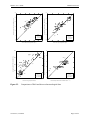
MOD12Q1 Landcover
Data from Previous Week
Spatial
&
tempora
l filling
è
è
Temporal filling
When no cloudyfree pixels of same
landcover
Filtering landcover
è
è
è
MOD15A2 QC
MOD15/17A2
MOD15/17A2
Filtering cloudy pixels
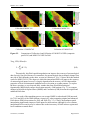
Figure 9.1.
Averaging cloud-free pixels
A schematic diagram illustrating the process of spatial and temporal interpolation
using information from land cover and QA flags. In this example, the landcover
map has only two values (dark and dashed pixels). In the bottom windows,
dark pixels are cloudy pixels, and white pixels are those with the best QA
conditions. The thick-bordered pixels are the pixels selected after filtering.
In temporal filling, data from the previous week is used to fill MOD15 or
MOD17A2.
Version 2.0, 12/2/2003
Page 34 of 57
MOD17 User’s Guide
MODIS Land Team
capture the effect of clouds on the local meteorology of any given pixel as DAO data is averaged
across the spatial domain of the data. There is nothing to be done at this point to account for
cloudiness in the DAO data. However, three interpolation methods for filling the GPP or
LAI/FPAR of cloudy pixels are suggested:
[1] fill the GPP of a cloudy pixel with GPP values from surrounding cloud-free
pixels
[2] fill the FPAR of a cloudy pixel with FPAR values from surrounding cloudfree pixels and then recompute the GPP of the cloudy pixel using the filled FPAR
[3] fill the FPAR and LAI of a cloudy pixel with FPAR and LAI values from surrounding
cloud-free pixels and recalculate the MOD17A2 algorithm.
The process of spatial and temporal interpolation is illustrated in Figure 9.1. When the central
pixel of a 5×5 moving window is cloudy, nearby cloud-free pixels with the same landcover are
used to interpolate the value of the central pixel. If there is no cloud-free pixel with a same
landcover within the moving window, the central pixel inherits the value from the preceding
week.
9.2. Data compositing
Currently, the MOD17A2 output is an 8-day summation product. However, in cloudy
areas such as the tropics, this scheme is not always sufficient, as there are times during the year
for which there are no cloud-free 8-day periods. As a result, researchers at NTSG are looking
into a 16-day summation, which might be more useful for exploring interannual differences in
GPP. This conversion will only occur if it provides an improved data stream. For those areas of
the earth’s land surface which are reasonably cloud-free, an 8-day summation may be continued.
9.3. Land cover
The land cover classification scheme ingested by the MOD17 Algorithm is at a 1-km
resolution as are all MODIS products. There are areas of the world, however, for which
improved, finer-resolution land cover data sets are available. Given the importance of accurate
land cover for the MOD17 algorithm, research is needed to determine if such data sets would
improve the MOD17 end products. For example, consideration is being given to using LandSatderived land cover with 15-m resolution in place of the MOD12Q1 Land Cover product in some
areas (Fig. 9.5). In this way, there would be a multi-resolution product that could increase the
accuracy of the MOD17 Algorithm. LandSat land cover data could provide enhanced spatial
resolution, while MODIS data (LAI/FPAR) provide the temporal resolution needed for the goals
set by the MODIS Science Team. LandSat-derived land cover hasn’t been used often for
productivity analysis in the past because of the long return-time (16-days) and cloudiness
associated with these products, but combining that land cover with the daily overpass of the
MODIS data could improve the MOD17A2 product. As with all MODIS products, MOD17
would continue to be produced at a 1-km resolution.
Version 2.0, 12/2/2003
Page 35 of 57
MOD17 User’s Guide
MODIS Land Team
TM 15m
panchromatic
MODIS 1km GPP
+
Figure 9.5.
Merged Image
→
Merging MODIS productivity data with high-resolution LandSat (TM) Data.
Version 2.0, 12/2/2003
Page 36 of 57
MOD17 User’s Guide
MODIS Land Team
CHAPTER II. PROPOSED IMPROVEMENTS TO THE
COLLECTION 4 ALGORITHM
1. Introduction
MODIS is the primary global monitoring sensor on the two NASA EOS satellites and
features improved geolocation, atmospheric correction and cloud screening provided by the
MODIS science team. MOD17 is a near real-time, continuous, consistent, operational data set of
global terrestrial gross primary productivity (GPP), and net primary productivity (NPP) at a 1km2 spatial scale, at both 8-day (MOD17A2) and annual (MOD17A3) time scales. Current
satellite data for MOD17 comes from the TERRA, EOS-AM platform, which was launched on
December 19, 1999. MOD17 began to provide 8-day estimates of GPP in December 2000. There
are currently almost 3 years of MODIS data available.
The MOD17 algorithm is based on the idea of the conservation ratio between APAR and
NPP, proposed by Monteith (1972), and the limitations of suboptimal environmental conditions
on the related conversion efficiency for different biome types. Detailed structure, and processes
of the algorithm can be found in Chapter I.
The objective of this Chapter is to provide users with a brief outline of the maturation of
MOD17 products from Collection 4 to Collection 4.5 (available upon request from NTSG), and
information on how Collection 4.5 improves the quality of MOD17 products. First, we provide a
retrospective view of the Collection 4 MOD17 algorithms and its problems; second, we show
how we have resolved these issues and improved MOD17. Finally, some results from Collection
4.5 are provided.
2. Problems with Collection 4 MOD17
To investigate the problems with the MOD17 algorithm, it is necessary to understand
how MOD17 operates (Fig. 2.1, Chapter I). For a given pixel, MOD17 requires two upstream
MODIS data inputs: MOD12Q1 and MOD15A2. The algorithm reads MOD12Q1 to obtain land
cover type to match the corresponding parameters in the Biome Parameter Look-Up Table
(BPLUT) (Table 2.1, Chapter I). The LAI/FPAR algorithm (MOD15A2) contains an 8-day
MVC (Maximum Value Composite) Fraction of Photosynthetic Active Radiation absorbed by
the green vegetation canopy (FPAR) and a corresponding Leaf Area Index (LAI). The MOD17
algorithm assumes that there is no variation of FPAR and LAI within a given 8-day period.
Outputs from MOD12Q1 and MOD15A2 provide real-time ground vegetation conditions. The
MOD17 algorithm also requires input of climate data to derive GPP and respiration. These data
are obtained from the DAO (Data Assimilation Office) (Atlas et al., 2000) modeled daily
meteorological obersvations as a 1° x 1.25° scale. At the end of each year, MOD17A3 (annual
NPP) is calculated from the 8-day MOD17A2, i.e., NPP is the summation of 8-day PsnNet minus
growth respiration.
There are two main problems with the Collection 4 MOD17 data set. The first is that, in
some cases, 8-day MVC MOD15A2 is still contaminated by clouds or other noise. As a result, in
regions with higher frequencies of cloud cover, such as tropical rain forests, values of FPAR and
Version 2.0, 12/2/2003
Page 37 of 57
MOD17 User’s Guide
MODIS Land Team
LAI will be greatly reduced (Fig. 2.1). To distinguish between good quality and contaminated
data, MOD15A2 contains Quality Control (QC) fields, which allow users to determine which
pixels are suitable for further analysis. The use of contaminated FPAR and LAI inputs will
produce incorrect 8-day GPP and PsnNet, and consequently, unreliable annual NPP. The second
problem arises from the use of DAO meteorological data in the algorithm. Currently, the DAO
data version used by MOD17 is GEOS402, which has a spatial resolution of 1° x 1.25°. All 1km2 MODIS pixels located within the same “large” DAO cell will use the same meteorological
data without spatial variation. In other words, each 1 km2 pixel retains the characteristics of the
nearest neighbor DAO cell. As a result, a DAO cell boundary line may appear in 1-km MOD17
images due to the relatively steep gradients between DAO cells (Fig. 2.2). Such treatment, on a
global or regional scale, may be acceptable, while at the local scale, especially for
topographically diverse terrain or sites located at relatively abrupt climatic gradient zones, it may
introduce inaccurate climatic predictions for some productivity calculations.
3. Improvements from Collection 4 to Collection 4.5
We solved the first problem related to MOD15A2 inputs by removing poor quality FPAR
and LAI data based on the QC label for every pixel. If any LAI/FPAR pixel does not meet the
quality screening criteria, its value is determined through linear interpolation between the
previous period’s value and that of the next good period. Fig. 2.1 illustrates how this temporal
filling approach is applied to a MODIS pixel in the Amazon region where higher frequency and
persistence of cloud cover exists. As depicted in Fig. 2.1, contaminated MOD15A2 was
improved as the result of the filling process. However, there are some unusual 8-day periods with
lower FPAR and LAI but good QC labels. In spite of this, we still depend on QC labeling as the
only source of quality control. Improved MOD15A2 leads to improvements of MOD17. Under
most conditions, 8-day composited GPP will increase because the temporal filling process
generally acts to increase FPAR. Changes in 8-day PsnNet, however, will depend on the changes
in both FPAR and LAI because improved MOD15A2 leads to increases in not only GPP but also
respiration (Equation 1.2, Chapter I). We found that in most regions, PsnNet increased in
Collection 4.5 relative to Collection 4. But for some small portions of the globe, PsnNet may not
change or may even be reduced as shown in Fig. 2.2.
For the second problem, arising from coarse spatial resolution daily DAO data, we use
spatial interpolation to enhance meteorological inputs. The four DAO cells nearest to a given 1km MODIS pixel are used in the interpolation algorithm. There are two reasons for choosing
four DAO cells per 1-km MODIS pixel:
[1] this will not slow down the computational efficiency of the MOD17 datastream,
which is a global product, and
[2] it is more reasonable to assume no elevation variation within four DAO cells than
any greater number of DAO cells.
We first attempted to use linear spatial interpolation, similar to the inverse distance weighting
(IDW) function commonly found in most GIS software. However, it failed because DAO
boundary lines remained. Instead we used non-linear interpolation. Although there are many
formulae for non-linear spatial interpolation, for simplicity, we use a cosine function because the
output value can be constrained between 0 and 1. This function still could not effectively
Version 2.0, 12/2/2003
Page 38 of 57
MOD17 User’s Guide
MODIS Land Team
1
7
6
0.8
LAI
Fpar
5
0.6
0.4
LAI_noQc
LAI_filling
1
FPAR_filling
0
0
0
60
120
180
8-day
240
300
0
360
12
8
10
6
8
4
6
PSN
GPP
3
2
FPAR_noQc
0.2
4
4
0
0
60
120
180
240
300
120
180
8-day
240
300
360
180
240
300
360
PSN_noQc
PSN_filling
2
0
GPP_noQc
GPP_filling
2
60
-2
360
0
60
120
-4
8-day
8-day
Figure 2.1.
Comparison of temporal profiles of 2001 Collection 4 MOD15A2 with original
values (FPAR_noQc, LAI_noQc) and temporally linearly-filled FPAR and LAI
(FPAR_filling, LAI_filling), and of temporal profiles of MOD17A2 with original
MOD15A2 inputs (GPP_noQc, PSN_noQc), and MOD17A2 with filled
MOD15A2 (GPP_filling, PSN_filling). The pixel is located in the Amazon
rainforest (lat = -1.0, lon = -60) with the MODIS land cover Evergreen Broadleaf
Forest (EBF).
eliminate DAO cell boundary lines in a MOD17 image, and thus we utilize a modified cosine
function of the form:
Di = cos 4 ((π / 2) * (d i / d max ))
i = 1,2,3,4
(2.1)
where Di is the non-linear distance between the 1-km MODIS pixel and any one of four
surrounding DAO cells; d i is the great-circle distance between the 1-km pixel and the same
DAO cell; and d max is the great-circle distance between the two farthest DAO cells of the four
being used. This ensures that Di = 1 when d i = 0, and Di = 0 when d i = d max . Based on the nonlinear distance ( Di ), the weighted value Wi can be expressed as
4
Wi = Di / ∑ Di ,
(2.2)
i =1
and therefore, for a given pixel, the corresponding smoothed value V (i.e., interpolated Tmin,
Version 2.0, 12/2/2003
Page 39 of 57
MOD17 User’s Guide
Collection 4 MOD17A2
Collection 4.5 MOD17A2
Figure 2.2.
MODIS Land Team
Collection 4 MOD17A3
Collection 4.5 MOD17A3
Comparison of Collection 4 and Collection 4.5 MOD17A2 GPP (composite
period 241) and MOD17A3 NPP for 2001.
Tavg, VPD, SWrad) is
4
V = ∑ (Wi * Vi )
(2.3)
i =1
Theoretically, this DAO spatial interpolation can improve the accuracy of meteorological
data for each 1-km pixel because it is unrealistic for meteorological data to abruptly change from
one side of DAO boundary to the other, as seen in Collection 4. Fig. 2.2 shows how this method
works for MOD17A2/A3. The degree to which this interpolated DAO will improve the accuracy
of meteorological inputs, however, is largely dependent on the accuracy of DAO data and the
properties of local environmental conditions such as elevation or weather patterns. To explore
the above question, we use observed daily weather data from World Meteorological
Organization (WMO) daily surface observation network (>5000 stations, Fig. 3.1) to compare
changes in Root Mean Squared Error (RMSE) and Correlation (COR) between the original and
enhanced DAO data.
As a result of the smoothing process, on average RMSE is reduced and COR increased
for 72.9% and 84% of the WMO stations, respectively, when comparing original and enhanced
DAO data to WMO observations for 2001 and 2002 (Fig. 3.2). Clearly, the nonlinear spatial
interpolation significantly improves DAO inputs for most stations, although for a few stations
interpolated DAO accuracy may be reduced due to the inaccuracy of DAO in these regions and
local conditions as noted above.
Version 2.0, 12/2/2003
Page 40 of 57
MOD17 User’s Guide
Figure 3.1.
MODIS Land Team
Distribution of more than 5,000 WMO stations for 2001 and 2002.
% stations with changed COR
% stations with changed RMSE
100
percent (%)
100
percent (%)
reduced (%)
increased (%)
50
50
0
0
Tmin RMSE Tavg RMSE AVP RMSE
variables
Figure 3.2.
VPD RMSE
Tmin R
Tavg R
AVP R
variables
VPD R
Percent of WMO stations with changes in RMSE and COR between spatially
interpolated and non-interpolated DAO. For most stations, DAO accuracies are
improved (reduced RMSE and increased COR) as a result of spatial interpolation.
Version 2.0, 12/2/2003
Page 41 of 57
MOD17 User’s Guide
MODIS Land Team
4. Addition of annual GPP and QC to Collection 4.5 MOD17A3
In an effort to make the MOD17A3 product more complete, we have added annual GPP
(summation of GPP) and a meaningful QC flag for NPP values. Currently, Collection 4
MOD17A3 has two layers in an HDFEOS file: NPP and NPP_QC (although this NPP_QC is
meaningless). We therefore define the MOD17A3 QC for a given pixel as
QC = (Periodsmissingandbad/Periodstotal)*100
(4.1)
where Periodsmissingandbad is the number of times linearly interpolated and Periodstotal is the total
number of 8-day composite periods during the growing season. The pixel with more periods of
filled MOD15A2 has a less reliable annual total for both GPP and NPP.
5. Final BPLUT applied to Collection 4.5 MOD17
The standard Collection 4 MOD17A2/A3 product is calculated using a BPLUT that was
calibrated to the GEOS3.0 DAO data set and Collection 3 MOD15A2, two primary inputs to the
MOD17 algorithm. The latest DAO (GEOS402) and MOD15A2 (Collection 4) have been
updated and improved. Given these enhanced inputs, the BPLUT (Table 2.1, Chapter I) has been
updated to improve global MOD17 outputs. This BPLUT for Collection 4.5 is based on recent
work by Nemani et al. (2003), observed GPP data from 13 flux towers in 2001 (Heinsch et al., in
prep), Ecosystem Model-Data Intercomparison (EMDI) NPP data (Olson et al., 2001), a recent
book summarizing global NPP (Roy et al., 2001), and additional publications (White et al., 2000;
Poorter et al., 2001; and Hoffmann et al., 2003).
6. Results
Improved MOD15A2 and improved DAO inputs together will enhance the MOD17
products. For example, even for North Dakota grasslands, which have a lower frequency of
cloud cover and smoother climatic gradients, r2 from Collection 4 to Collection 4.5, increased
from 0.54 to 0.77 in 2001 and from 0.50 to 0.57 in 2002 for the relationship between clipped
herbaceous biomass in July and integrated MOD17 PsnNet from Composite Period 1 through
193 (Reeves, et al., in prep), indicating Collection 4.5 significantly improves NPP compared to
Collection 4.
Several of the corrections discussed in this Chapter cannot be performed in a forwardprocessing mode. Therefore, at the end of each year the data from that year will be reprocessed
to include the corrections, such as linear interpolation of the MOD15A2 input data. While we
feel that Collection 4.5 data are the most accurate data, users should balance their research needs
with data availability to determine the product that fits their needs. The standard Collection 4.0
product will continue to be available in near real-time. Currently, Collection 4.5 data are
available for 2001-2002. Additional data will be released as they become available.
~ The global Collection 4.5 image gallery can be found at http://www.ntsg.umt.edu. Data
from Collection 4.5(2001-2002) are available upon request from NTSG.
Version 2.0, 12/2/2003
Page 42 of 57
MOD17 User’s Guide
MODIS Land Team
CHAPTER III. ORDERING MOD17A2 DATA
1. Naming Conventions
In order to efficiently take advantage of the Earth Observing System Data Gateway
(EDG) it is useful to understand the naming convention for the MODIS granule ID. The granule
names are a combination of several pieces of key information, which will help you to discern if
the granule in question is what you desire.
From Figure 1, we see that the local granule ID (see the EDG web user’s guide for a
definition; http://edcimswww.cr.usgs.gov/pub/imswelcome/ ) contains much information about
the data stored therein. The product short name tells us that we are looking at MODIS GPP data
from the Terra Satellite.
MOD17A2 Naming Convention
Product version
number
Data format
identifier
MOD17A2.A2001009.h10v04.004.2003217234300.hdf
Tile location
on grid
Product short
name
Processing year,
date and time
Acquisition
Date
Figure 1.1.
The MOD17A2 Standard Product naming convention.
The acquisition date is simply the year and yearday, indicating when the data was collected. The
next field indicates the horizontal and vertical positions associated with the data granule (these
numbers are related to the map projection of the data; see Fig 5.1). The product version number
shows which version of the production software was used to generate the data. The processing
information tells you the year, date and time when the processing was run on the data present in
the granule. The format identifier simply tells you what type of file format the data is stored in.
2. Logging into the EDG
When you first bring up the EDG web site
(http://edcimswww.cr.usgs.gov/pub/imswelcome/) in your browser you will be greeted by a page
similar to that in Figure 2.1. You can either enter as a guest or as a registered user. If you wish
to become a registered user you may click on the appropriate link. If you do not wish to become
Version 2.0, 12/2/2003
Page 43 of 57
MOD17 User’s Guide
Figure 2.1.
MODIS Land Team
The EDG home page.
a registered user, you are still able to order data as a guest, although you will not be able to save
any searches or user information.
3. Searching the Data
3.1. EDG search page
The search page (Fig. 3.1) consists of several fields, in which you enter the information
on which you want to search. Since the EDG has an extensive online help system and several
tutorials, here we will only cover what you need to know to order MOD17A2 data.
First you will have to specify which data set you wish to search for. In this case you will
want to enter 'MOD17A2' in the field labeled ‘Method 1: Data Set Lookup’. Then just click on
the button labeled GO. The screen will change slightly to display the results of the data set
search. You should see something like 'MODIS/TERRA NET PHOTOSYNTHESIS 8-DAY L4
GLOBAL 1KM ISIN GRID V003'. You want to select the most recent version of the data unless
Version 2.0, 12/2/2003
Page 44 of 57
MOD17 User’s Guide
Figure 3.1.
MODIS Land Team
The EDG search page.
your research restricts you to an older version. Be sure to document which version you are
using. In this case it is version 3 (V003).
Next you must choose your search area. You can do this in several ways, by typing in
latitude and longitude, choosing a global search, or by selecting the area you wish to search from
Version 2.0, 12/2/2003
Page 45 of 57
MOD17 User’s Guide
Figure 3.2.
MODIS Land Team
Choosing the time range.
a java applet (you must have a java enabled browser for this approach). This is fairly
straightforward.
Next you need to choose the time range of your search. To do this you may enter the date
in normal or standard date range (YYYY-MM-DD), Julian date range (YYYY-DDD) or you can
do an annually repeating time range (Fig. 3.1 and Fig. 3.2). After indicating the time range you
must make sure that you have allowed the search engine to return the proper number of results.
This is done by entering the number of granules to return in the field entitled, 'Return a
Maximum of <blank> data granules'. The maximum number of granules that can be returned, at
the time of this writing, are 1000 (Fig. 3.2).
Not much more is required to get MOD17A2 data; just click on the start button and
you’re in business!
3.2 Search In Progress page
This page shows you the results of the search as it is happening. If there are any errors
this page will indicate them with 'Error' in the status field. The status field will also tell you
Version 2.0, 12/2/2003
Page 46 of 57
MOD17 User’s Guide
MODIS Land Team
the back button on the browser and correct the issue.
Figure 3.3.
The “Search in progress” page.
when your search is successful and the other fields will give you more information, including
number of granules returned (Fig. 3.3). Some errors on this page will be in the form of server
errors, caused by neglecting to fill in a required field on the search page. If this happens just hit
3.3. Granule listing page
The granule-listing page lists the granules that were returned as a result of your search.
This page also gives you the choice of adding the granules to your shopping cart. Using this
Version 2.0, 12/2/2003
Page 47 of 57
MOD17 User’s Guide
MODIS Land Team
page, you may select some or all of the granules by clicking the checkboxes in the desired
granules row (Fig. 3.4). Once you have selected your granules, you must add them to your cart.
3.4. Disclaimer page
After your data are found, the EDG will display a disclaimer (Fig. 3.5). This page is
displayed because of the current state of the MODIS data stream. MODIS data are still being
evaluated and validated. If you wish to continue, click the ‘Accept’ button at the bottom of the
page.
Figure 3.4.
The page listing the granules you have requested.
Version 2.0, 12/2/2003
Page 48 of 57
MOD17 User’s Guide
Figure 3.5.
MODIS Land Team
The disclaimer.
4. Ordering the Data
4.1 Ordering options page
The ordering options page is very similar to the granule-listing page. You are shown
your granules (10 at a time) and you may choose the ordering options for them one at a time or
all at once. For our purposes just click on Choose Options (Fig. 4.1). This will take you to the
second part of the ordering options page.
4.2. Ordering options page (part II)
The second half of the ordering options page allows you to select the method of data
transfer (Fig. 4.2). For our purposes select FtpPull. Then mark the selection box, which states
you wish to use this option for all the granules of this data set (Fig. 4.2). Then press the OK
button.
Version 2.0, 12/2/2003
Page 49 of 57
MOD17 User’s Guide
Figure 4.1.
MODIS Land Team
Choosing ordering options.
This will take you, once again, back to the Ordering Options page. You will notice a change,
however (Fig. 4.3). The words 'FtpPull' and 'Change Options' will appear next to each row
displayed on the page. This is telling you that these granules are ready to be ordered. Be careful
here! If you are ordering more than one data set (say MOD17A2 and MOD17A3) not all of your
granules are ready. The display shows 10 granules at a time. Read the page carefully to find on
which page the second data set starts and click on that button (the numbered buttons on the
bottom of the page (1-10....). Fore each extra data set, repeat the steps for data retrieval that were
covered previously and then you proceed to the next section.
To move forward in the ordering process press the 'Go to Step 2: Order Form' button.
Version 2.0, 12/2/2003
Page 50 of 57
MOD17 User’s Guide
Figure 4.2.
MODIS Land Team
Choosing ordering options, part II.
Version 2.0, 12/2/2003
Page 51 of 57
MOD17 User’s Guide
Figure 4.3.
MODIS Land Team
Choosing ordering options, the “Ready” page.
4.3. Order form
In this step you will fill out the order form telling the specific D.A.A.C. (Distributed
Active Archive Center) how to get in touch with you via e-mail regarding your request and data
availability. If you have any questions concerning this form read the online tutorial, or contact
the EDG's help desk. When you are done click on the button, which will take you to step 3 of
the ordering process (Fig. 4.4).
Version 2.0, 12/2/2003
Page 52 of 57
MOD17 User’s Guide
Figure 4.4.
MODIS Land Team
The order form.
4.4. Reviewing your order (Step 3)
This step gives you a summary of what you have accomplished thus far. Since MODIS
data are available at no cost to the public, the total cost should amount to US $0.00. If everything
is satisfactory just click the button that allows you to continue on to the next step, ‘Submit
Order’ (Fig. 4.5).
4.5. Submitting the order
Once you have submitted the order, you will see a screen similar to the search in progress
page. This will notify you if any errors occurred while contacting the data center which houses
the data you requested. Once this step is complete, you will see a page stating that your order
was submitted, with a comprehensive listing of what you ordered.
You will receive e-mail notification of your request at the address you provided in the
order page. You will also receive a notification via e-mail when your order is being filled. This
last notification is important because it tells you from where you need to get your data (ftp
address, directory where the data are stored, file names). If you have any other questions, please
utilize the materials at the EDG’s web site (http://edcimswww.cr.usgs.gov/pub/imswelcome/).
Version 2.0, 12/2/2003
Page 53 of 57
MOD17 User’s Guide
Figure 4.5.
MODIS Land Team
Verifying and submitting the order.
5. The DataPool:
The DataPool was developed as an alternative distribution point for EOS data. The
DataPool is a large disk cache where EOS data are temporarily stored after they are inserted at
the DAAC. What is stored in this area depends upon usage. The primary benefit of using the
DataPool is that data can be more quickly retrieved. For more information please see
http://lpdaac2.usgs.gov/datapool/datapool.asp.
! Please see the DataPool located at the DAAC you are using for specific access instructions
as they may differ among DAAC’s. (Please note: The above URL will take you to the Land
Processes DAAC DataPool page.)
Version 2.0, 12/2/2003
Page 54 of 57
MOD17 User’s Guide
MODIS Land Team
MODIS FAQ’s
There are many MODIS related FAQ’s available on the internet. Perhaps the most
comprehensive of these is located at: http://daac.gsfc.nasa.gov/MODIS/FAQ/.
MOD17A2/A3 FAQ
1. How much do MODIS data cost?
Nothing. MODIS data are free.
2. What units are my data in?
The MOD17A2/A3 data are in units of kg C m-2 day. However, you must apply a scale
factor of 0.0001 to each pixel to obtain these units.
3. What is the difference between PSN_1km and GPP?
There is no difference.
4. What is the difference between Gpp_1km and PSNnet_1km?
PSNnet_1km is equal to Gpp_1km MINUS the maintenance respiration from leaves and
fine roots. In other words, Gpp_1km should always be ≥ PSNnet_1km at any given pixel.
5. What criteria do you use to create quality assurance (QA) for the annual net primary
productivity (NPP) product?
The QA values are inherited from the final 8-day composite period in any given year
from the MOD15 LAI/FPAR input data.
Version 2.0, 12/2/2003
Page 55 of 57
MOD17 User’s Guide
MODIS Land Team
REFERENCES
Atlas, R.M., Lucchesi, R. (2000), File Specific for GEOS-DAS Celled Output, Goddard Space
Flight Center, Greenbelt, Maryland.
Belward, A., J. Estes, et al. (1999). "The IGBP-DIS Global 1-km Land-Cover Data Set
DISCover: A Project Overview." Photogrammetric Engineering & Remote Sensing
65: 1013-1020.
Campbell, N. A. (1990). Biology. Redwood City, CA, The Benjamin/Cummings Publishing
Company, Inc.
Cannell, M. (1982). World Forest Biomass and Primary Production Data. London, Academic
Press.
Field C.B., J.T. Randerson, and C.M. Malmstrom (1995). "Global net primary production:
Combining ecology and remote sensing." Remote Sensing of the Environment
281: 237-240.
Goward, S., C. Tucker, et al. (1985). "North American vegetation patterns observed with the
NOAA-7 advanced very high resolution radiometer." Vegetatio 64: 3-14.
Hansen, M., R. DeFries, et al. (2000). "Global land cover classification at the 1km spatial
resolution using a classification tree approach." International Journal of Remote Sensing
21: 1331-1364.
Heinsch, F.A., S.W. Running, et al. (in prep). "Validation of the MOD17A2 GPP product using
eddy covariance flux tower data."
Hoffmann, W. A. and A.C. Franco (2003). “Comparative growth analysis of tropical forest and
savanna woody plants using phylogenetically independent contrasts.” Journal of Ecology
91: 475-484
Hunt, E. J. (1994). "Relationship between woody biomass and PAR conversion efficiency for
estimating net primary production from NDVI." International Journal of Remote Sensing
15: 1725-1730.
Maier, C., S. Zarnoch, et al. (1998). "Effects of temperature and tissue nitrogen on dormant
season stem and branch maintenance respiration in a young loblolly pine (Pinus taeda)
plantation." Tree Physiology 18(1): 11-20.
Monteith, J. (1972). "Solar radiation and productivity in tropical ecosystems." Journal of Applied
Ecology 9: 747-766.
Monteith, J. (1977). "Climate and efficiency of crop production in Britain." Philosophical
Transactions of the Royal Society of London, Ser. B: 277-294.
Nemani, R.R., C.D. Keeling, et al. (2003). “Climate-Driven Increases in Global Terrestrial Net
Primary Production from 1982 to 1999.” Science. 300: 1560-1563.
Olson, R. J., K. R. Johnson, et al. (2001). “Global and Regional Ecosystem Modeling: Databases
of Model Drivers and Validation Measurements” ORNL/TM-2001/196. 1-84
Poorter, L. (2001). “Light-dependent changes in biomass allocation and their importance for
growth of rain forest tree species.” Functional Ecology 15:1123-123.
Prince, S. and S. Goward (1995). "Global primary production: a remote sensing approach."
Journal of Biogeography 22(4/5): 815-835.
Reeves MR, Zhao M, Heinsch FA and Running SW. (in prep). Characterizing moisture driven
rangeland biomass fluctuations using MODIS primary productivity estimates.
Reich, P., B. Kloeppel, et al. (1995). "Different photosynthesis-nitrogen relations in deciduous
hardwood and evergreen coniferous tree species." Oecologia 104(1): 24-30.
Version 2.0, 12/2/2003
Page 56 of 57
MOD17 User’s Guide
MODIS Land Team
Reich, P., M. Walters, et al. (1994). "Photosynthesis-nitrogen relations in Amazonian tree
species. I. Patterns among species and communities." Oecologia 97(1): 24-30.
Roy, J., B. Saugier, and H.A. Mooney, ed. (2001). “Terrestrial global productivity.” Academic
Press, San Diego, CA.
Running, S. and E. J. Hunt (1993). Generalization of a forest ecosystem process model for other
biomes, BIOME-BGC, and an application for global-scale models. Modeling Sustainable
Forest Ecosystems. D. C. L. a. R.A.Sedjo. Washington, DC, American Forests: 1-15.
Running, S.W., P. E. Thornton, et al. (2000). Global terrestrial gross and net primary
productivity from the Earth Observing System. Methods in Ecosystem Science. O. Sala,
R. Jackson and H. Mooney. New York, Springer Verlag: 44-57.
Running, S.W.,
Scepan, J. (1999). "Validation of High-Resolution Global Land-Cover Data Sets."
Photogrammetric Engineering & Remote Sensing 65: 1051-1060.
Schubert, S., R. Rood, et al. (1993). "An assimilated dataset for earth science applications."
Bulletin of the American Meteorological Society 74: 2331-2342.
Schwarz, P., T. Fahey, et al. (1997). "Seasonal air and soil temperature effects on photosynthesis
in red spruce (Picea rubens) saplings." Tree Physiology 17(3): 187-194.
Thornton, P.E., B.E. Law, et al. (2002). "Modeling and measuring the effects of disturbance
history and climate on carbon and water budgets in evergreen needleleaf forests."
Agricultural and Forest Meteorology 113: 185-222.
Turner, D.P., S. Urbanski, et al. (2003). "A cross-biome comparison of daily light-use efficiency
for gross primary production" Global Change Biology 9:383-395.
Waring, R.H. and S.W. Running (1998). "Forest Ecosystems: Analysis at Multiple Scales:
Academic Press, San Deigo, CA.
White, M., P. Thornton, et al. (2000). "Parameterization and Sensitivity Analysis of the BIOME–
BGC Terrestrial Ecosystem Model: Net Primary Production Controls." Earth Interactions
4.
Wolfe R. E., M. Nishihama, A. J. Fleig, J. R. Kuyper, D. P. Roy, J. C. Storey, F. S. Patt (2002).
“Achieving sub-pixel geolocation accuracy in support of MODIS land science.” Remote
Sensing of Environment 83(1-2): 31-49.
Version 2.0, 12/2/2003
Page 57 of 57