Download A User's Guide to gringo, clasp, clingo, and iclingo - Multi

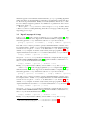
A User’s Guide to
gringo, clasp, clingo, and iclingo ∗
(version 3.x)
Martin Gebser
Roland Kaminski
Benjamin Kaufmann
Max Ostrowski
Torsten Schaub
Sven Thiele ∗∗
October 4, 2010
— Preliminary Draft —
Abstract
This document provides an introduction to the Answer Set Programming (ASP)
tools gringo, clasp, clingo, and iclingo, developed at the University of
Potsdam. The first tool, gringo, is a grounder capable of translating logic programs provided by users into equivalent propositional logic programs. The answer
sets of such programs can be computed by clasp, which is a solver. The third
tool, clingo, integrates the functionalities of gringo and clasp, thus, acting
as a monolithic solver for user programs. Finally, iclingo extends clingo
by an incremental mode that incorporates both grounding and solving. For one,
this document aims at enabling ASP novices to make use of the aforementioned
tools. For another, it provides a reference of their features that ASP adepts might
be tempted to exploit.
Note that this document contains a lot of examples. For convienience no
examples have to be typed in by hand instead they can directly be safed to disc
by clicking them.
∗ Tools
gringo, clasp, clingo, and iclingo are available at [46].
∗∗ {gebser,kaminski,kaufmann,ostrowsk,torsten,sthiele}@cs.uni-potsdam.de
1
Contents
1
Introduction
4
2
Quickstart
2.1 Problem Instance . . . . . . . . . . . . . . . . . . . . . . . . . . . .
2.2 Problem Encoding . . . . . . . . . . . . . . . . . . . . . . . . . . .
2.3 Problem Solution . . . . . . . . . . . . . . . . . . . . . . . . . . . .
6
6
7
8
3
Input Languages
3.1 Input Language of gringo and clingo . . . . .
3.1.1 Normal Programs and Integrity Constraints
3.1.2 Classical Negation . . . . . . . . . . . . .
3.1.3 Disjunction . . . . . . . . . . . . . . . . .
3.1.4 Built-In Arithmetic Functions . . . . . . .
3.1.5 Built-In Comparison Predicates . . . . . .
3.1.6 Assignments . . . . . . . . . . . . . . . .
3.1.7 Intervals . . . . . . . . . . . . . . . . . . .
3.1.8 Conditions . . . . . . . . . . . . . . . . .
3.1.9 Pooling . . . . . . . . . . . . . . . . . . .
3.1.10 Aggregates . . . . . . . . . . . . . . . . .
3.1.11 Optimization . . . . . . . . . . . . . . . .
3.1.12 Meta-Statements . . . . . . . . . . . . . .
3.1.13 Integrated Scripting Language . . . . . . .
3.2 Input Language of iclingo . . . . . . . . . . . .
3.3 Input Language of clasp . . . . . . . . . . . . .
.
.
.
.
.
.
.
.
.
.
.
.
.
.
.
.
.
.
.
.
.
.
.
.
.
.
.
.
.
.
.
.
.
.
.
.
.
.
.
.
.
.
.
.
.
.
.
.
.
.
.
.
.
.
.
.
.
.
.
.
.
.
.
.
.
.
.
.
.
.
.
.
.
.
.
.
.
.
.
.
.
.
.
.
.
.
.
.
.
.
.
.
.
.
.
.
.
.
.
.
.
.
.
.
.
.
.
.
.
.
.
.
.
.
.
.
.
.
.
.
.
.
.
.
.
.
.
.
.
.
.
.
.
.
.
.
.
.
.
.
.
.
.
.
.
.
.
.
.
.
.
.
.
.
.
.
.
.
.
.
9
9
9
11
12
12
13
14
14
16
17
18
22
23
26
29
31
Examples
4.1 N -Coloring . . . . . . . .
4.1.1 Problem Instance .
4.1.2 Problem Encoding
4.1.3 Problem Solution .
4.2 Traveling Salesperson . . .
4.2.1 Problem Instance .
4.2.2 Problem Encoding
4.2.3 Problem Solution .
4.3 Blocks-World Planning . .
4.3.1 Problem Instance .
4.3.2 Problem Encoding
4.3.3 Problem Solution .
.
.
.
.
.
.
.
.
.
.
.
.
.
.
.
.
.
.
.
.
.
.
.
.
.
.
.
.
.
.
.
.
.
.
.
.
.
.
.
.
.
.
.
.
.
.
.
.
.
.
.
.
.
.
.
.
.
.
.
.
.
.
.
.
.
.
.
.
.
.
.
.
.
.
.
.
.
.
.
.
.
.
.
.
.
.
.
.
.
.
.
.
.
.
.
.
.
.
.
.
.
.
.
.
.
.
.
.
.
.
.
.
.
.
.
.
.
.
.
.
.
.
.
.
.
.
.
.
.
.
.
.
.
.
.
.
.
.
.
.
.
.
.
.
.
.
.
.
.
.
.
.
.
.
.
.
.
.
.
.
.
.
.
.
.
.
.
.
.
.
.
.
.
.
.
.
.
.
.
.
.
.
.
.
.
.
.
.
.
.
.
.
.
.
.
.
.
.
.
.
.
.
.
.
.
.
.
.
.
.
.
.
.
.
.
.
.
.
.
.
.
.
.
.
.
.
.
.
.
.
.
.
.
.
.
.
.
.
.
.
.
.
.
.
.
.
.
.
.
.
.
.
.
.
.
.
.
.
.
.
.
.
.
.
.
.
.
.
.
.
.
.
.
.
.
.
32
32
32
33
33
34
34
35
36
37
37
38
39
Command Line Options
5.1 gringo Options . . . . .
5.2 clingo Options . . . . .
5.3 iclingo Options . . . .
5.4 clasp Options . . . . . .
5.4.1 General Options .
5.4.2 Search Options . .
5.4.3 Lookback Options
.
.
.
.
.
.
.
.
.
.
.
.
.
.
.
.
.
.
.
.
.
.
.
.
.
.
.
.
.
.
.
.
.
.
.
.
.
.
.
.
.
.
.
.
.
.
.
.
.
.
.
.
.
.
.
.
.
.
.
.
.
.
.
.
.
.
.
.
.
.
.
.
.
.
.
.
.
.
.
.
.
.
.
.
.
.
.
.
.
.
.
.
.
.
.
.
.
.
.
.
.
.
.
.
.
.
.
.
.
.
.
.
.
.
.
.
.
.
.
.
.
.
.
.
.
.
.
.
.
.
.
.
.
.
.
.
.
.
.
.
.
.
.
.
.
.
.
.
.
.
.
.
.
.
.
.
.
.
.
.
.
40
40
41
42
43
43
45
46
4
5
2
6
Errors and Warnings
6.1 Errors . . . . . . . . . . . . . . . . . . . . . . . . . . . . . . . . . .
6.2 Warnings . . . . . . . . . . . . . . . . . . . . . . . . . . . . . . . .
47
47
49
7
Future Work
49
References
50
A Differences to the Language of lparse
54
List of Figures
1
2
3
4
5
6
Towers of Hanoi Initial Situation . . . . . . . . .
Terms . . . . . . . . . . . . . . . . . . . . . . .
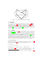
A Directed Graph with Six Nodes and 17 Edges.
A 3-Coloring for the Graph in Figure 3. . . . . .
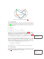
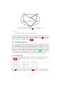
The Graph from Figure 3 along with Edge Costs.
A Minimum-Cost Round Trip. . . . . . . . . . .
.
.
.
.
.
.
.
.
.
.
.
.
.
.
.
.
.
.
.
.
.
.
.
.
.
.
.
.
.
.
.
.
.
.
.
.
.
.
.
.
.
.
.
.
.
.
.
.
.
.
.
.
.
.
.
.
.
.
.
.
.
.
.
.
.
.
6
10
32
33
34
36
.
.
.
.
.
.
.
.
.
.
.
.
.
.
.
.
.
.
.
.
.
.
.
.
.
.
.
.
.
.
.
.
.
.
.
.
.
.
.
.
.
.
.
.
.
.
.
.
.
.
.
.
.
.
.
.
.
.
.
.
.
.
.
.
.
.
.
.
.
.
.
.
.
.
.
.
.
.
.
.
.
.
.
.
.
.
.
.
.
.
.
.
.
.
.
.
.
.
.
.
.
.
.
.
.
.
.
.
.
.
.
.
.
.
.
.
.
.
.
.
.
.
.
.
.
.
.
.
.
.
.
.
.
.
.
.
.
.
.
.
.
.
.
.
.
.
.
.
.
.
.
.
.
.
.
.
.
.
.
.
.
.
.
.
.
.
.
.
.
.
.
.
.
.
.
.
.
.
.
.
.
.
.
.
.
.
.
.
.
.
.
.
.
.
.
.
.
.
.
.
.
.
.
.
.
.
.
.
.
.
.
.
.
.
.
.
.
.
.
.
.
.
.
.
.
.
.
.
.
.
.
.
.
.
.
.
.
.
.
.
.
.
.
.
.
.
.
.
.
.
.
.
.
.
.
.
.
.
.
.
.
.
.
.
11
12
13
13
14
14
15
16
16
17
17
19
22
26
27
28
30
32
33
34
35
35
37
38
Listings
examples/flycn.lp . .
examples/arithf.lp . .
examples/arithc.lp . .
examples/symbc.lp .
examples/assign.lp .
examples/unify.lp . .
examples/int.lp . . .
examples/cond.lp . .
examples/twocond.lp
examples/pool.lp . .
examples/sep.lp . . .
examples/aggr.lp . .
examples/opt.lp . . .
examples/luaf.lp . . .
examples/luav.lp . . .
examples/sql.lp . . .
examples/inc.lp . . .
examples/graph.lp . .
examples/color.lp . .
examples/costs.lp . .
examples/ham.lp . .
examples/min.lp . . .
examples/world0.lp .
examples/blocks.lp .
.
.
.
.
.
.
.
.
.
.
.
.
.
.
.
.
.
.
.
.
.
.
.
.
.
.
.
.
.
.
.
.
.
.
.
.
.
.
.
.
.
.
.
.
.
.
.
.
.
.
.
.
.
.
.
.
.
.
.
.
.
.
.
.
.
.
.
.
.
.
.
.
.
.
.
.
.
.
.
.
.
.
.
.
.
.
.
.
.
.
.
.
.
.
.
.
.
.
.
.
.
.
.
.
.
.
.
.
.
.
.
.
.
.
.
.
.
.
.
.
.
.
.
.
.
.
.
.
.
.
.
.
.
.
.
.
.
.
.
.
.
.
.
.
.
.
.
.
.
.
.
.
.
.
.
.
.
.
.
.
.
.
.
.
.
.
.
.
.
.
.
.
.
.
.
.
.
.
.
.
.
.
.
.
.
.
.
.
.
.
.
.
.
.
.
.
.
.
.
.
.
.
.
.
.
.
.
.
.
.
.
.
.
.
.
.
.
.
.
.
.
.
.
.
.
.
.
.
.
.
.
.
.
.
.
.
.
.
.
.
3
.
.
.
.
.
.
.
.
.
.
.
.
.
.
.
.
.
.
.
.
.
.
.
.
.
.
.
.
.
.
.
.
.
.
.
.
.
.
.
.
.
.
.
.
.
.
.
.
.
.
.
.
.
.
.
.
.
.
.
.
.
.
.
.
.
.
.
.
.
.
.
.
.
.
.
.
.
.
.
.
.
.
.
.
.
.
.
.
.
.
.
.
.
.
.
.
.
.
.
.
.
.
.
.
.
.
.
.
.
.
.
.
.
.
.
.
.
.
.
.
.
.
.
.
.
.
.
.
.
.
.
.
.
.
.
.
.
.
.
.
.
.
.
.
.
.
.
.
.
.
.
.
.
.
.
.
.
.
.
.
.
.
.
.
.
.
.
.
.
.
.
.
.
.
.
.
.
.
.
.
.
.
.
.
.
.
.
.
.
.
.
.
1
Introduction
The “Potsdam Answer Set Solving Collection” (Potassco) [46] by now gathers a variety
of tools for Answer Set Programming. Among them, we find grounder gringo, solver
clasp, and combinations thereof within integrated systems clingo and iclingo.
All these tools are written in C++ and published under GNU General Public License(s) [30]. Source packages as well as precompiled binaries for Linux and Windows
are available at [46]. For building one of the tools from sources, please download the
most recent source package and consult the included README or INSTALL text file,
respectively. Please make sure that the platform to build on has the required software
installed. If you nonetheless encounter problems in the building process, please use
the potassco mailing list [email protected] or consult the supporting pages at potassco.sourceforge.net.
After downloading (and possibly building) a tool, one can check whether everything works fine by invoking the tool with flag --version (to get version information) or with flag --help (to see the available command line options). For instance,
assuming that a binary called gringo is in the path (similarly, with the other tools),
the following command line calls should be responded by gringo:
gringo --version
gringo --help
If grounder gringo, solver clasp, as well as integrated systems clingo and
iclingo are all available, one usually provides the file names of input text files to either gringo, clingo, or iclingo, while the output of gringo is typically piped
into clasp. Thus, the standard invocation schemes are as follows:
gringo [ options | files ] | clasp [ options | number ]
clingo [ options | files | number ]
iclingo [ options | files | number ]
Note that a numerical argument provided to either clasp, clingo, or iclingo
determines the maximum number of answer sets to be computed, where 0 stands for
“compute all answer sets.” By default, only one answer set is computed (if it exists).
This guide introduces the fundamentals of using gringo, clasp, clingo, and
iclingo. In particular, it tries to enable the reader to benefit from them by significantly reducing the “time to solution” on difficult problems. The outline is as follows.
In Section 2, an introductory example is given that serves both as guideline on how
to model problems using logic programs and also as an example on how compact and
concise the modeling language of gringo is. The probably most important part for a
user, Section 3, is dedicated to the input languages of our tools, where the joint input
language of gringo and clingo claims the main share (later on, it is extended by
iclingo). For illustrating the application of our tools, three well-known example
problems are solved in Section 4. Practical aspects are also in the focus of Section 5
and 6, where we elaborate and give some hints on the available command line options
as well as input-related errors and warnings that may be reported. During the guide
we forgo most of the theoretical background in favor of small intuitive examples and
informal descriptions.
For readers familiar with lparse [53] (a grounder that constitutes the traditional
front end of solver smodels [51]), Appendix A lists the most prominent differences
to our tools. Otherwise, gringo, clingo, and iclingo should accept most inputs
recognized by lparse, while the input of solver clasp can also be generated by
4
lparse instead of gringo. Throughout this guide, we provide quite a number of
examples. Many of them can actually be run, and instructions on how to accomplish
this (or sometimes meta-remarks) are provided in margin boxes, where an occurrence
of “\” usually means that a text line broken for space reasons is actually continuous.
After all these preliminaries, it is time to start our guided tour through Potassco [46].
We hope that you will find it enjoyable and helpful!
5
a
b
4
3
2
1
c
4
3
2
1
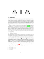
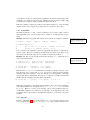
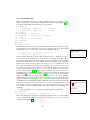
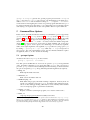
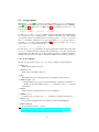
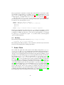
Figure 1: Towers of Hanoi Initial Situation
2
Quickstart
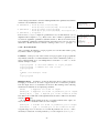
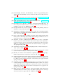
In this section we demonstrate the expressive power and the simple yet powerful modeling language of gringo by looking at the simple Towers of Hanoi puzzle. It consists
of three pegs and a set of discs of different sizes, which can be put onto the pegs. The
goal is to move all pegs from the leftmost peg to the rightmost peg, where at each time
only the topmost disc can be moved on top of another peg. Additionally, a disc may not
be put on top of a smaller disc. We ignore that there is an efficient algorithm to solve
this problem and just specify how a solution, in terms of a sequence of moves, has to
look.
In ASP it is custom to provide a uniform problem definition [39, 42, 50]. Following
this methodology, we separate the encoding from an instance of the following problem:
given an initial placement of the discs, a goal situation, and a number n, decide whether
there is a sequence of moves of length n that satisfies the conditions given above.
We will see that this decision problem can be elegantly specified by reducing it to a
declarative problem solving paradigm like ASP, where efficient off-the-shelf tools like
gringo and clasp are ready to solve the problem reasonably well. Such a reduction
is now exemplified.
2.1
Problem Instance
We consider a Towers of Hanoi instance specified via facts over predicates peg/1 and
disk/1 that correspond to the pegs and disks in the puzzle. Discs are enumerated by
consecutive integers beginning with one, where a disc with a lower number is considered to be bigger than a disc with a higher number. The pegs can have arbitrary
names. Furthermore, the predicates init on/2 and goal on/2 describe the initial
and goal situation, respectively. Their first argument is the number of a disc and the
second argument is the peg on which the disc is located in the initial or goal situation.
Finally, the predicate moves/1 specifies the number of moves within which the goal
situation has to be reached. Note that the original puzzle had exactly three pegs and a
fixed initial and goal situation. With ASP we can easily change this requirement and
the encoding represented in the following works with an arbitrary number of pegs and
any initial or goal situation. Figure 1 depicts a possible instance (the dashed discs mark
the goal situation) corresponding to the ASP program given below.
1
2
3
4
5
peg(a;b;c).
disk(1..4).
init_on(1..4,a).
goal_on(1..4,c).
moves(15).
6
The “;” in the first line is some syntactic sugar (Section 3.1.9) that expands the
statement into three facts peg(a), peg(b), and peg(c) representing the three pegs.
Again, in the second line some syntactic sugar is used to create the facts disc(1),
disc(2), disc(3), and disc(4). Here the term 1..4, an intervall (Section
3.1.7), is successively replaced by 1, 2, 3, and 4. The initial and goal situation is
specified in line three and four again using intervall. Finally, in the last line the number
of moves to solve the problem is given.
2.2
Problem Encoding
We now proceed by encoding the Towers of Hanoi puzzle via non-ground rules (Section
3.1.1), i.e, rules with variables that are independent of particular instances. Typically,
an encoding consists of a Generate, a Define, and a Test part [36]. We follow this
paradigm and mark respective parts via comment lines beginning with % in the encoding below. The variables D, P, T, and M are used to refer to disks, pegs, the T-th move
in the sequence of moves, and the length of the sequence, respectively.
1
2
3
4
5
6
7
8
9
10
11
12
13
14
15
16
% Generate
1 { move(D,P,T) : disk(D) : peg(P) } 1 :- moves(M), T = 1..M.
% Define
move(D,T)
:- move(D,_,T).
on(D,P,0)
:- init_on(D,P).
on(D,P,T)
:- move(D,P,T).
on(D,P,T+1) :- on(D,P,T), not move(D,T+1), not moves(T).
blocked(D-1,P,T+1) :- on(D,P,T), disk(D), not moves(T).
blocked(D-1,P,T)
:- blocked(D,P,T), disk(D).
% Test
:- move(D,P,T), blocked(D-1,P,T).
:- move(D,T), on(D,P,T-1), blocked(D,P,T).
:- goal_on(D,P), not on(D,P,M), moves(M).
:- not 1 { on(D,P,T) : peg(P) } 1, disk(D), moves(M), T = 1..M.
#hide.
#show move/3.
The Generate part consists of just one rule in Line 2. At each time point T at which
a move is executed, we “guess” exactly one move that puts an arbitrary disk to some
arbitrary peg. The head of this rule is a so called cardinality constraint (Section 3.1.10)
that consists of a set that is expanded using the predicates behind the colons (Section
3.1.8) and a lower and an upper bounds. The constraint is true if and only if the number
of true literals within the set is between the upper and lower bound. Furthermore, the
constraint is used in the head of a rule, that is, it is not only a test but can derive
(“guess”) new atoms, which in this case correspond to possible moves of discs. Note
that at this point we have not constrained the moves. Up to now, any disc could be
moved to any peg at each time point with out considering any problem constraints.
Next follows the Define part, here we give rules that define new auxiliary predicates, which as such do not touch the satisfiability of the problem but are used in the
Test part later on. The rule in Line 4 projects out the target peg of a move, i.e., the
predicate move/2 can be used if we only need the disc affected by a move but not its
target location. We use the predicate on/3 to capture the state of the Hanoi puzzle at
each time point. Its first two argument give the location of a disc at the time point
given by the third argument. The next rule in Line 5 infers the location of each disc
7
in the initial state (time point 0). Then we model the state transition using the rules
in Line 6 and 7. The first rule is quite straightforward and states that the moved disc
changes its location. Note the usage of not moves(T) here. This literal prevents
deriving an infinite number of rules, which would be all useless because the state no
longer changes after the last move. The second rule makes sure that all discs that are
not moved stay where they are. Finally, we define the auxiliary predicate blocked/3,
which marks positions w.r.t. pegs that cannot be moved from. First in Line 8, the position below a disc on some peg is blocked. Second in Line 9, the position directly below
a blocked position is blocked. Note that we mark position zero to be blocked, too. This
is convenient later on to assert some redundant moves.
Finally, there is the Test part building upon both Generate and Define part to rule
out wrong moves that do not agree with the problem description. It consists solely of
integrity constraints, which fail whenever all their literals are true. The first integrity
constraint in Line 11 asserts that a disc that is blocked, i.e, with some disc on top,
cannot be moved. Note the usage of D-1 here, this way a disc cannot be put back to the
same location again. The integrity constraint in Line 12 asserts that a disc can only be
placed on top of a bigger disc. Line 13 asserts the goal situation. To make the encoding
more efficient, we add a redundant constraint in Line 14, which asserts that each disc at
all time points is located on exactly one peg. Although, this constraint is implied by the
constraints above, adding this additional domain knowledge greatly improves the speed
with which the problem can be solved. Finally, the last two statements control which
predicates are printed, when a satisfying model for the instance is found. Here we first
hide all predicates (Line 15) and then explicitly show only the move/3 predicate (Line
16).
2.3
Problem Solution
Now we are ready to solve the encoded puzzle. To find an answer set, invoke one
of the following commands (clingo, or gringo and clasp have to be installed
somewhere under the systems path for the commands below to work):
clingo inst_toh.lp enc_toh.lp
gringo inst_toh.lp enc_toh.lp | clasp
Note that (depending on your viewer) you can right or double-click on file names
marked with a red font to safe the associated file to disc. This is possible with all
examples given in this document.
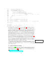
The output of the solver (clingo in this case) looks something like that:
Answer: 1
move(4,b,1)
move(4,a,5)
move(4,c,9)
move(4,b,13)
SATISFIABLE
Models
Time
Prepare
Prepro.
Solving
:
:
:
:
:
move(3,c,2)
move(3,b,6)
move(3,a,10)
move(3,c,14)
move(4,c,3) move(2,b,4) \
move(4,b,7) move(1,c,8) \
move(4,a,11) move(2,c,12) \
move(4,c,15)
1+
0.010
0.000
0.010
0.000
8
The first line indicates that an answer set follows in the line below (the \ marks
a line wrap). Then the status follows, this might be either SATISFIABLE,
UNSATISFIABLE, or UNKNOW if the computation is interrupted. The 1+ right of
Models: indicates that one answer set has been found and the + that the whole search
space has not yet been explored, so there might be further answer sets. Following that,
there are some time measurements: Beginning with total computation time, which is
split into preparation time (grounding), preprocessing time (clasp has an internal preprocessor that tries to simplify the program), and solving time (the time needed to find
the answer excluding preparation and preprocessing time). More information about
options and output can be found in Section 5.
3
Input Languages
This section provides an overview of the input languages of grounder gringo, combined grounder and solver clingo, incremental grounder and solver iclingo, and
of solver clasp. The joint input language of gringo and clingo is detailed in
Section 3.1. It is extended by iclingo with a few directives described in Section 3.2.
Finally, Section 3.3 is dedicated to the inputs handled by clasp.
3.1
Input Language of gringo and clingo
The tool gringo [26] is a grounder capable of translating logic programs provided
by users into equivalent ground programs. The output of gringo can be piped into
solver clasp [20], which then computes answer sets. System clingo internally
couples gringo and clasp, thus, it takes care of both grounding and solving. In
contrast to gringo outputting ground programs, clingo returns answer sets.
Usually logic programs are specified in one or more text files whose names are
passed via the command line in an invocation of either gringo or clingo. We
below provide a description of constructs belonging to the input language of gringo
and clingo.
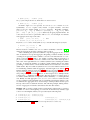
3.1.1
Normal Programs and Integrity Constraints
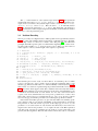
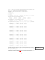
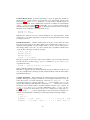
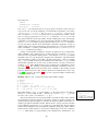
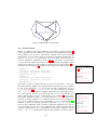
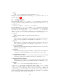
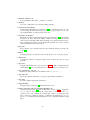
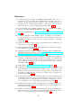
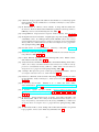
Every logic program is constructed from terms. An overview of gringo terms is depicted in Figure 2. The most basic terms are integers, constants, and variables. Furthermore, there are some special variables and constants. An anonymous variable denoted
by ‘ ’ is simialar to a normal variable but each occurrence is treated like a different
variable (intuitively a new unique variable name is substituted). Additionally, there
are the two special constants ‘#supremum’ and ‘#infimum’ representing the largest and
the smallest possible values, respectively, which behave essentially like constants. Finally, there are function symbols which are composed of other terms. A term that does
not contain any (anonymous) variables is called a ground term. More complex terms
involving arithmetics and other constructs are introduced later on.
Rules are defined as follows:
Rule:
Fact:
Integrity Constraint:
A0 :- L1 , . . . ,Ln .
A0 .
:- L1 , . . . ,Ln .
9
constant
[a-z]
[A-Za-z0-9]
variable
[A-Z]
[A-Za-z0-9]
simpleterm
integer
constant
variable
#supremum
#infimum
function
constant
(
simpleterm
)
,
term
simpleterm
function
Figure 2: Terms
10
simpleterm
The head A0 of a fact or a rule is an atom of the same form as a function symbol
or constant. Any Lj is a literal of the form A or not A for an atom A where the
connective not corresponds to default negation. The set of literals {L1 , . . . , Ln } is
called the body of the rule. Facts have an empty body. Throughout this section we
further extend the predicates that can be used in a rule including comparison predicates
(Section 3.1.5) and aggregates (Section 3.1.10). Furthermore, gringo expects rules
to be safe, i.e., all variables that appear in a rule have to appear in some positive literal
(a literal not preceded by not) in the body. If a variable appears positively in some
predicate, then we say that this predicate binds the variable.
Intuitively, the head of a rule has to be true whenever all its body literals are true.
In ASP every atom needs some derivation, i.e., an atom cannot be true if there is no
rule deriving it. This implies that only atoms appearing in some head can appear in
answer sets. Furthermore, derivations1 have to be acyclic, a feature that is important
to model reachability. As a simple example, consider the program a :- b. b :a. The only answer set to this program is the empty set. Adding either a. or b.
to the program results in the answer set {a, b}. Finally, note that default negation is
ignored when checking for acyclic derivations (we do not need a reason for an atom
being false). Default negation can be used to express choices, e.g., the program a :not b. b :- not a. has the two answer sets {a} and {b}. But in practice it is
never needed to express choices this way. For example in the introductory example in
Section 2 we used a cardinality constraint, which provides a much more readable way
to introduce choices.
A fact has an empty body and thus its associated head predicate is always true and
appears in all answer sets. On the other hand, integrity constraints eliminate answer set
candidates. They are merely tests that discard unwanted answer sets. That is, there are
no answer sets that satisfy all literals an integrity constraint. Elaborate examples on the
usage of facts, rules, and integrity constraints are provided in Section 4.
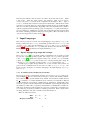
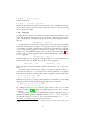
3.1.2
Classical Negation
In logic programs, connective not expresses default negation, that is, a literal not A
is assumed to hold unless A is derived. In contrast, the classical (or strong) negation of
some proposition holds if the complement of the proposition is derived [27]. Classical
negation, indicated by symbol “-,” is permitted in front of atoms. That is, if A is an
atom, then -A is the complement of A. Semantically, -A is simply a new atom, with
the additional condition that A and -A must not jointly hold. Observe that classical
negation is merely a syntactic feature that can be implemented via integrity constraints
whose effect is to eliminate any answer set candidate containing complementary atoms.
Example 3.1. Consider a logic program comprising the following facts:
1
2
bird(tux).
bird(tweety).
3
4
5
flies(X) :- bird(X), not -flies(X).
-flies(X) :- bird(X), not flies(X).
-flies(X) :- penguin(X).
penguin(tux).
chicken(tweety).
Logically, classical negation is reflected by (implicit) integrity constraints as follows:
1 There are extensions like disjunctions that go beyond simple derivability and also require minimality
w.r.t. a reduct. We do not cover the semantics of such constraints in this guide.
11
By invoking
gringo -t \
bird.lp flycn.lp
the reader can observe that
gringo indeed produces the
integrity constraint in Line 7.
6
7
:- flies(tux),
-flies(tux).
:- flies(tweety), -flies(tweety).
The program has two answer sets. One contains flies(tweety) and the other
contains -flies(tweety). Let us now add a new fact to the program:
8
flies(tux).
There no longer is any answer set for our new program using classical negation. In fact,
answer set candidates that contain both flies(tux) and -flies(tux) violate the
integrity constraint in Line 6.
3.1.3
Disjunction
Disjunctive logic programs permit connective “|” between atoms in rule heads. A
disjunction is true if at least one of its atoms is true. Additionally, logic programs
have to satisfy a minimality criterion, which we do not detail in this guide. The simple
program a | b. has the two answer sets {a} and {b} but does not admit the answer
set a, b because it is no minimal model.
In general, the use of disjunction however increases computational complexity [12].
This is why clingo2 and solvers like assat [37], clasp [20], nomore++ [1],
smodels [51], and smodelscc [56] do not work on disjunctive programs. Rather,
claspD [8], cmodels [28, 35], or gnt [33] need to be used for solving a disjunctive
program.3 We thus suggest to use “choice constructs” (cf. Section 3.1.10) instead of
disjunction, unless the latter is required for complexity reasons (see [13] for an implementation methodology in disjunctive ASP).
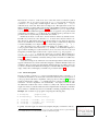
3.1.4
Built-In Arithmetic Functions
gringo and clingo support a number of arithmetic functions that are evaluated
during grounding. The following symbols are used for these functions: + (addition), (subtraction, unary minus), * (multiplication), / or #div (integer division), \ or #mod
(modulo function), ** or #pow (exponentation), |·| or #abs (absolute value), &
(bitwise AND), ? (bitwise OR), ˆ (bitwise exclusive OR), and ˜ (bitwise complement).
Example 3.2. The usage of arithmetic functions is illustrated by the logic program:
1
2
3
4
5
6
7
8
9
10
11
12
13
left
right
plus
minus
uminus
times
divide1
divide2
divide2
modulo1
modulo2
modulo3
absolute1
2 Run
(7).
(2).
(L +
R )
(L R )
(
- R )
(L *
R )
(L /
R )
(R #div L )
(#div(R,L))
(L \
R )
(L #mod R )
(#mod(L,R))
(
|- R|)
:::::::::::-
left(L), right(R).
left(L), right(R).
right(R).
left(L), right(R).
left(L), right(R).
left(L), right(R).
left(L), right(R).
left(L), right(R).
left(L), right(R).
left(L), right(R).
right(R).
as a monolithic system performing both grounding and solving.
but it uses a different syntax than presented here.
3 System dlv [34] also deals with disjunctive programs,
12
The unique answer set of the
program, obtained after evaluating all arithmetic functions,
can be inspected by invoking:
gringo -t arithf.lp
14
15
16
17
18
19
20
21
absolute2
power1
power2
power2
bitand
bitor
bitxor
bitneg
(#abs(- R))
(L ** R )
(L #pow R )
(#pow(L,R))
(L &
R )
(L ?
R )
(L ˆ
R )
(
˜ R )
::::::::-
left(L),
left(L),
left(L),
left(L),
left(L),
left(L),
right(R).
right(R).
right(R).
right(R).
right(R).
right(R).
right(R).
right(R).
Note that variables L and R are instantiated to 7 and 2, respectively, before arithmetic evaluations. Consecutive and non-separative (e.g., before “(”) spaces can also
be dropped, while spaces after tokens #div and #mod are mandatory. Furthermore,
the argument of function #abs, #div, and #mod must be enclosed in parentheses.
The four bitwise functions apply to signed integers, using the two’s complement of a
negative integer.
Note that it is important that variables in the scope of an arithmetic function are not
bound by a corresponding atom. For instance, the rule p(X) :- p(X+1). is
not safe but p(X-1) :- p(X). is. Although, the latter might produce an infinite
grounding and gringo not necessarily halts when given such an input.
3.1.5
Built-In Comparison Predicates
The following built-in predicates permit term comparisons within the bodies of rules:
== (equal), != (not equal), < (less than), <= (less than or equal), > (greater than), >=
(greater than or equal).
Example 3.3. The usage of comparison predicates is illustrated by the logic program: The unique answer set of the
1
2
3
4
5
6
7
8
9
num(1).
eq (X,Y)
neq(X,Y)
lt (X,Y)
leq(X,Y)
gt (X,Y)
geq(X,Y)
all(X,Y)
non(X,Y)
num(2).
:- X
== Y,
:- X
!= Y,
:- X
<
Y,
:- X
<= Y,
:- X
>
Y,
:- X
>= Y,
:- X-1 < X+Y,
:- X/X > Y*Y,
program is obtained via call:
gringo -t arithc.lp
num(X),
num(X),
num(X),
num(X),
num(X),
num(X),
num(X),
num(X),
num(Y).
num(Y).
num(Y).
num(Y).
num(Y).
num(Y).
num(Y).
num(Y).
The last two lines hint at the fact that arithmetic functions are evaluated before comparison predicates, so that the latter actually compare integers.
All comparison predicates can also be used with arbitrary ground terms, as in the
next program:
As above, invoking:
1
2
3
4
5
6
7
sym(1).
eq (X,Y)
neq(X,Y)
lt (X,Y)
leq(X,Y)
gt (X,Y)
geq(X,Y)
sym(a).
:- X ==
:- X !=
:- X <
:- X <=
:- X >
:- X >=
sym(f(a)).
Y, sym(X),
Y, sym(X),
Y, sym(X),
Y, sym(X),
Y, sym(X),
Y, sym(X),
sym(Y).
sym(Y).
sym(Y).
sym(Y).
sym(Y).
sym(Y).
Integers are compared in the usual way and constants are ordered lexicographically.
Function symbols are compared first using their arity. If the arity differs, then the name
13
gringo -t symbc.lp
yields the unique answer set of
the program in terms of facts.
of the function symbol is compared lexicographically. If again the name differs, then
arguments are compared component wise. Finally, integers are always smaller than
constants and constants are always smaller than function symbols.
Note that a built-in comparison predicate cannot bind variables, i.e., when checking
whether a rule is safe, comparison predicates are not considered to be positive.
3.1.6
Assignments
The built-in predicates := and = can be used in the body of a rule to unify a term on
their right-hand side to a (non-ground) term or variable on its left-hand side, respectively.
Example 3.4. The next program demonstrates how terms can be assigned to variables: The unique answer set of the
1
num(1).
3
4
5
squares(XX,YY,Z) :XX := X*X, YY := Y*Y, Z := XX+YY, Y1 := Y+1,
Y1*Y1 == Z, num(X), num(Y), X < Y.
num(2).
num(3).
num(4).
program is obtained via call:
gringo -t assign.lp
num(5).
Line 3 contains four assignments, where the right-hand sides directly or indirectly depend on X and Y. These two variables are bound in Line 5 via atoms of predicate num/1.
Also observe the different usage and role of built-in comparison predicate ==.
Example 3.5. The second program demonstrates the usage of :=, which allows for
terms on the left hand side:
The unique answer set of the
1
2
sym(f(a,1,2)). sym(f(a,1,3)). sym(f(b,d)).
sym((a,1,2)). sym((a,1,3)). sym((b,d)).
4
5
unifyf(X) :- f(a,X,X+1) := F, sym(F).
unifyt(X) :- (a,X,X+1) := T, sym(T).
program is obtained via call:
gringo -t unify.lp
Here the term f(a,X,X+1) is unified with every function symbol provided by sym/1.
Note the usage of X+1 in the term. gringo does not try to unify any term containing
arithmetic but in this example X occurs also directly as second argument of the argument and can thus be unified with. The term X + 1 is merely a test that is deferred and
checked later. For example, the fourth line is equivalent to:
6
unifyf(X) :- f(a,X,Y) := F, sym(F), Y == X + 1.
Note that assignments to some extent can bind variables. Of course cyclic assignments
cannot bind variables. For example the rule p(X) :- X = Y, Y = X. is rejected
by gringo. Either X or Y has to be provided by some positive predicate in this case.
Additionally, unification is restricted to ground terms on the right hand side of the
assignment, that is, all variables on the right hand side have to be bound by some other
predicate.
3.1.7
Intervals
In Line 1 of Example 3.4, there are five facts num(k) over consecutive integers k. For
a more compact representation, gringo and clingo support integer intervals of the
14
form i..j, where i and j are integers. Such an interval represents each integer k such
that i ≤ k ≤ j, and intervals are expanded during grounding.
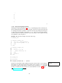
Example 3.6. The next program makes use of integer intervals:
1
2
3
4
num(1..5).
top5(5..9).
top(9).
top5num(1..X-4,5..X) :- num(X-4..X), top5(1..5), top(X).
The facts in Line 1 and 2 are expanded as follows:
num(1).
top5(5).
num(2).
top5(6).
num(3).
top5(7).
num(4).
top5(8).
num(5).
top5(9).
By instantiating X to 9, the rule in Line 4 becomes:
top5num(1..5,5..9) :- num(5..9), top5(1..5), top(9).
It is expanded to the cross product (1..5) × (5..9) × (5..9) × (1..5) of intervals:
top5num(1,5)
top5num(2,5)
.
.
.
top5num(5,5)
top5num(1,6)
top5num(2,6)
.
.
.
. .
.
top5num(5,9)
top5num(1,5)
top5num(2,5)
.
.
.
. .
.
top5num(5,9)
top5num(1,5)
top5num(2,5)
.
.
.
. .
.
top5num(5,9)
top5num(1,5)
top5num(2,5)
.
.
.
. .
.
top5num(5,9)
top5num(1,5)
top5num(2,5)
.
.
.
. .
.
top5num(5,9)
:- num(5), top5(1), top(9).
:- num(5), top5(1), top(9).
:- num(5), top5(1), top(9).
:- num(5), top5(1), top(9).
:- num(5), top5(1), top(9).
:- num(5), top5(1), top(9).
:- num(6), top5(1), top(9).
:- num(6), top5(1), top(9).
.
.
.
:- num(9), top5(1), top(9).
:- num(5), top5(2), top(9).
:- num(5), top5(2), top(9).
.
.
.
.
.
.
:- num(9), top5(4), top(9).
:- num(5), top5(5), top(9).
:- num(5), top5(5), top(9).
:- num(5), top5(5), top(9).
:- num(6), top5(5), top(9).
:- num(6), top5(5), top(9).
.
.
.
:- num(9), top5(5), top(9).
Note that only the rules with num(5) and top5(5) in the body actually contribute to Again the unique answer set is
the unique answer set of the above program by deriving all atoms top5num(m,n) obtained via call:
gringo -t int.lp
for 1 ≤ m ≤ 5 and 5 ≤ n ≤ 9.
Note that as with built-in arithmetic functions, an integer interval mentioning some
variable (like X in Line 4 of Example 3.6) cannot be used to bind the variable.
15
3.1.8
Conditions
Conditions allow for instantiating variables to collections of terms within a single rule.
This is particularly useful for encoding conjunctions or disjunctions over arbitrarily
many ground atoms as well as for the compact representation of aggregates (cf. Section 3.1.10). The symbol “:” is used to formulate conditions.
Example 3.7. The following program uses conditions in a rule body and in a rule head:
1
2
3
4
5
6
person(jane). person(john).
day(mon). day(tue). day(wed). day(thu). day(fri).
available(jane) :- not on(fri).
available(john) :- not on(mon), not on(wed).
meet :- available(X) : person(X).
on(X) : day(X) :- meet.
We are particularly interested in the rules in Line 5 and 6, instantiated as follows:
5
6
meet :- available(jane), available(john).
on(mon) | on(tue) | on(wed) | on(thu) | on(fri) :- meet.
The conjunction in Line 5 is obtained by replacing X in available(X) with all The reader can reproduce these
ground terms t such that person(t) holds, namely, t = jane and t = john. ground rules by invoking:
Furthermore, the condition in the head of the rule in Line 6 turns into a disjunction gringo -t cond.lp
over all ground instances of on(X) where X is substituted by some term t such that
day(t) holds. That is, conditions in the body and in the head of a rule are expanded
to different basic language constructs.
Composite conditions can also be constructed via “:,” as in the additional rules:
7
8
9
day(sat). day(sun).
weekend(sat). weekend(sun).
weekdays :- day(X) : day(X) : not weekend(X).
Observe that we may use the same atom, viz., day(X), both on the left-hand and on
the right-hand side of “:.” Furthermore, negative literals like not weekend(X) can
occur on both sides of a condition. Note that literals on the right-hand side of a condition are connected conjunctively, that is, all of them must hold for ground instances of
an atom in front of the condition. Thus, the instantiated rule in Line 8 looks as follows:
8
weekdays :- day(mon), day(tue), day(wed), day(thu), day(fri).
The atoms in the body of this rule follow from facts, so that the rule can be simplified
to a fact weekdays. (as done by gringo).
Note that there are three important issues about the correct usage of conditions:
1. All predicates of atoms on the right-hand side of a condition must be either domain predicates,i.e., predicates that can be completely evaluated during grounding, or built-in, which is due to the fact that conditions are evaluated during
grounding.
2. Any variable occurring within a condition is considered as local, that is, a condition cannot be used to bind variables outside the condition. In turn, variables
outside conditions are global, and each variable within an atom in front of a
condition must occur on the right-hand side or be global.
16
3. Global variables take priority over local ones, that is, they are instantiated first.
As a consequence, a local variable that also occurs globally is substituted by
a term before the ground instances of a condition are determined. Hence, the
names of local variables must be chosen with care, making sure that they do not
accidentally match the names of global variables.
3.1.9
Pooling
Symbol “;” allows for pooling alternative terms to be used as argument within an atom,
thus, specifying rules more compactly. An atom written in the form p(. . . ,X;Y,. . . )
abbreviates two options: p(. . . ,X,. . . ) and p(. . . ,Y,. . . ). Pooled arguments in
any term of a rule body (or on the right-hand side of a condition) are expanded to
a conjunction of the options within the same body (or within the same condition),
while they are expanded to multiple rules (or multiple literals connected via “,”) when
occurring in the head (or in front of a condition).
Example 3.8. The following logic program makes use of pooling:
1
2
3
4
sym(a). sym(b).
num(1). num(2).
mix(A;B,M;N) :- sym(A;B), num(M;N), not -mix(M;N,A;B).
-mix(M;N,A;B) :- sym(A;B), num(M;N), not mix(A;B,M;N).
Let us consider instantiations of the rule in Line 3 obtained with substitution {A 7→ a,
B 7→ b, M 7→ 1, N 7→ 2}. Note that mix/2 and -mix/2 each admit four options, corresponding to the cross product of {a, b} substituted for A and B, respectively, together
with {1, 2} substituted for M and N. While the instances obtained for mix/2 give rise
to four rules, the instances for -mix/2 jointly belong to the body. The (repeated) body
also contains two instances each of sym/1 and of num/1. We thus get the rules:
Simplified versions of these
mix(a,1) :- sym(a),sym(b), num(1),num(2), not -mix(1,a),
not -mix(1,b), not -mix(2,a), not -mix(2,b).
mix(a,2) :- sym(a),sym(b), num(1),num(2), not -mix(1,a),
not -mix(1,b), not -mix(2,a), not -mix(2,b).
mix(b,1) :- sym(a),sym(b), num(1),num(2), not -mix(1,a),
not -mix(1,b), not -mix(2,a), not -mix(2,b).
mix(b,2) :- sym(a),sym(b), num(1),num(2), not -mix(1,a),
not -mix(1,b), not -mix(2,a), not -mix(2,b).
rules are produced via call:
gringo -t pool.lp
Additionally, there is the ;; operator for pooling, which can only be used to separate arguments of predicates. This operator does not work on single terms but simply
lists arguments of predicates. The rules for expanding the predicates are the same as
for the ; operator.
Example 3.9. The following example show the difference between the ; and ;; operator:
Simplified versions of these
1
2
3
rules are produced via call:
gringo -t sep.lp
p(1,2). p(2,3).
p(X,Z) :- p(X,Y;;Y,Z).
q(X,Z) :- q(X,Y;Y,Z).
The second line is expanded into the following:
17
2
p(X,Z) :- p(X,Y), p(Y,Z).
and the third line into:
3
p(X,Z) :- p(X,Y,Z), p(X,Y,Z).
Clearly, the first variant is the desired expansion in this case to calculate the transitive
closure. Both operators have their usages in different scenarios to keep the encoding
more compact and readable.
3.1.10
Aggregates
An aggregate is an operation on a multiset of weighted literals that evaluates to some
value. In combination with comparisons, we can extract a truth value from an aggregate’s evaluation, thus, obtaining an aggregate atom. We consider aggregate atoms of
the form:
l op [ L1 =w1 , . . . ,Ln =wn ] u
An aggregate has a lower bound l, an upper bound u, an operation op, and a multiset
of literal Li each assigned to a weight wi . An aggregate is true if operation op applied
to the multiset of weights of true literals is between the bounds (inclusive). Currently,
gringo supports the aggregates #sum (the sum of weights), #min (the minimum
weight), #max (the maximum weight), and #avg (the average of all weights 4 ). Furthermore, there are three aggregates that are syntactically different. The first is the
#count aggregate:
l #count { L1 , . . . ,Ln } u
which basically are #sum aggregates with all weights set to one and duplicate true
literals counted only once. Finally, there are the two parity aggregates:
#even { L1 , . . . ,Ln }
#odd { L1 , . . . ,Ln }
These aggregates are true if the number of different true literals is even or odd, respectively.
As regards syntactic representation, weight 1 is considered a default, so that Li =1
can simply be written as Li . For instance, the following (multi)sets of (weighted)
literals are the same when combined with any kind of aggregate operation and bounds:
[a=1, not b=1, c=2] and
[a,
not b,
c=2].
Furthermore, keyword #sum may be omitted, which in a sense makes #sum the default
aggregate operation. In fact, the following aggregate atoms are synonyms:
2 #sum [a, not b, c=2] 3 and
2
[a, not b, c=2] 3.
By omitting keyword #sum, we obtain the same notation as the one of so-called
“weight constraints” [51, 53], which are actually aggregate atoms whose operation
is addition.
It is important to note that the (weighted) literals within an aggregate belong to a
multiset. In particular, if there are multiple occurrences L=w1 , . . . , L=wk of a literal L,
in combination with #min and #max, it is not the same like having L=w1 + · · · + wk .
To see this, note that the program consisting of the facts:
4 The average aggregate over an empty set of weights is defined to be always true irrespective of any
bounds.
18
2 #max [a=2].
2 #min [a=2].
has {a} as its unique answer set, while there is no answer set for:
2 #max [a,a].
2 #min [a,a].
If literals ought not to be repeated, we can use #count instead of #sum.
Syntactically, #count requires curly instead of square brackets, and there
must not be any weights within a #count aggregate. Regarding semantics,
(l #count { L1 , . . . ,Ln } u) reduces to (l sum [ L1 =1, . . . ,Lm =1 ] u), where
{L1 , . . . , Lm } = {Li | 1 ≤ i ≤ n} is obtained by dropping repeated literals. Of
course, the use of l and u is optional also with #count. As an example, note that the
next aggregate atoms express the same:
1 #sum
[a=1, not b=1]
1 and
1 #count {a,a, not b,not b} 1.
Keyword #count can be omitted (like #sum), so that the following are synonyms:
1 #count {a, not b} 1 and
1
{a, not b} 1.
The last notation is similar to the one of so-called “cardinality constraints” [51, 53],
which are aggregate atoms using counting as their operation.
After considering the syntax and semantics of ground aggregate atoms, we now
turn our attention to non-ground aggregates. Regarding contained variables, an atom
occurring in an aggregate behaves similar to an atom on the left-hand side of a condition (cf. Section 3.1.8). That is, any variable occurring within an aggregate is a
priori local, and it must be bound via a variable of the same name that is global or
that occurs on the right-hand side of a condition (with the atom containing the variable
in front). As with local variables of conditions, global variables take priority during
grounding, so that the names of local variables must be chosen with care to avoid accidental clashes. Beyond conditions (which are more or less the natural construct to use
for instantiating variables within an aggregate), classical negation (cf. Section 3.1.2),
built-in arithmetic functions (cf. Section 3.1.4), intervals (cf. Section 3.1.7), and pooling (cf. Section 3.1.9) can be incorporated as usual within aggregates, where intervals
and pooling are expanded locally.5 That is, an interval gives rise to multiple literals
connected via “,” within the same aggregate. The same applies to pooling in front of
a condition, while it turns into a composite condition chained by “:” on the right-hand
side. Finally, note that aggregates #sum, #count, #min, and #max without bounds
are also permitted on the right-hand sides of assignments, but using this feature is only
recommended for aggregates whose atoms belong to domain predicates because space
blow-up can become a bottleneck otherwise. The following example, making exhaustive use of aggregates, nonetheless demonstrates this and other features.
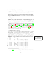
Example 3.10. Consider a situation where an informatics student wants to enroll for
a number of courses at the beginning of a new term. In the university calendar, eight
courses are found eligible, and they are represented by the following facts:
1
2
3
4
course(1,1,5). course(1,2,5).
course(2,1,4). course(2,2,4).
course(3,1,6).
course(3,3,6).
course(4,1,3).
course(4,3,3). course(4,4,3).
5 Assignments
(cf. Section 3.1.6) are permitted on the right-hand sides of conditions only.
19
5
6
7
8
course(5,1,4).
course(5,4,4).
course(6,2,2). course(6,3,2).
course(7,2,4). course(7,3,4). course(7,4,4).
course(8,3,5). course(8,4,5).
In an instance of course/3, the first argument is a number identifying one of the eight
courses, and the third argument provides the course’s contact hours per week. The second argument stands for a subject area: 1 corresponding to “theoretical informatics,”
2 to “practical informatics,” 3 to “technical informatics,” and 4 to “applied informatics.” For instance, atom course(1,2,5) expresses that course 1 accounts for 5
contact hours per week that may be credited to subject area 2 (“practical informatics”).
Observe that a single course is usually eligible for multiple subject areas.
After specifying the above facts, the student starts to provide personal constraints
on the courses to enroll. The first condition is that 3 to 6 courses should be enrolled:
9
3 { enroll(C) : course(C,_,_) } 6.
Instantiating the above #count aggregate yields the following ground rule:
9
3 { enroll(1), enroll(2), enroll(3), enroll(4),
enroll(5), enroll(6), enroll(7), enroll(8) } 6.
The full ground program is obtained by invoking:
gringo -t aggr.lp
Observe that an instance of atom enroll(C) is included for each instantiation of C
such that course(C,S,H) holds for some values of S and H. Duplicates resulting
from distinct values for S are removed, thus, obtaining the above set of ground atoms.
The next constraints of the student regard the subject areas of enrolled courses:
10 :- [ enroll(C) : course(C,_,_) ] 10.
11 :- 2 [ not enroll(C) : course(C,2,_) ].
12 :- 6 [ enroll(C) : course(C,3,_), enroll(C) : course(C,4,_) ].
Each of the three integrity constraints above contains a sum aggregate, using default
weight 1 for literals. Recalling that #sum aggregates operate on multisets, duplicates
are not removed. Thus, the integrity constraint in Line 10 is instantiated as follows:
10 :- [ enroll(1)
enroll(2)
enroll(3)
enroll(4)
enroll(5)
enroll(6)
enroll(7)
enroll(8)
=
=
=
=
=
=
=
=
1,
1,
1,
1,
1,
1,
1,
1,
enroll(1)
enroll(2)
enroll(3)
enroll(4)
enroll(5)
enroll(6)
enroll(7)
enroll(8)
=
=
=
=
=
=
=
=
1,
1,
1,
1, enroll(4) = 1,
1,
1,
1, enroll(7) = 1,
1 ] 10.
Note that courses 4 and 7 count three times because they are eligible for three subject areas, viz., there are three distinct instantiations for S in course(4,S,3) and
course(7,S,4), respectively. Comparing the above ground instance, the meaning
of the integrity constraint in Line 10 is that the number of eligible subject areas over all
enrolled courses must be more than 10. Similarly, the integrity constraint in Line 11
expresses the requirement that at most one course of subject area 2 (“practical informatics”) is not enrolled, while Line 12 stipulates that the enrolled courses amount to
less than six nominations of subject area 3 (“technical informatics”) or 4 (“applied
informatics”). Also note that, given the facts in Line 1–8, we could equivalently have
used count rather than sum in Line 11, but not in Line 10 and 12.
20
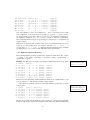
The remaining constraints of the student deal with contact hours. To express them,
we first introduce an auxiliary rule and a fact:
13 hours(C,H) :- course(C,S,H).
14 max_hours(20).
The rule in Line 13 projects instances of course/3 to hours/2, thereby, dropping
courses’ subject areas. This is used to not consider the same course multiple times
within the following integrity constraints:
15 :- not M-2 [ enroll(C) : hours(C,H) = H ] M, max_hours(M).
16 :- #min [ enroll(C) : hours(C,H) = H ] 2.
17 :- 6 #max [ enroll(C) : hours(C,H) = H ].
As Line 15 shows, we may use default negation via “not” in front of aggregate atoms,
and bounds may be specified in terms of variables. In fact, by instantiating M to 20, we
obtain the following ground instance of the integrity constraint in Line 15:
15 :- not 18 [ enroll(1)
enroll(3)
enroll(5)
enroll(7)
=
=
=
=
5,
6,
4,
4,
enroll(2)
enroll(4)
enroll(6)
enroll(8)
=
=
=
=
4,
3,
2,
5 ] 20.
The above integrity constraint states that the #sum of contact hours per week must lie
in-between 18 and 20. Note that the #min and #max aggregates in Line 16 and 17,
respectively, work on the same (multi)set of weighted literals as in Line 15. While the
integrity constraint in Line 16 stipulates that any course to enroll must include more
than 2 contact hours, the one in Line 17 prohibits enrolling for courses of 6 or more
contact hours. Of course, the last two requirements could also be formulated as follows:
16 :- enroll(C), hours(C,H), H <= 2.
17 :- enroll(C), hours(C,H), H >= 6.
Finally, the following rules illustrate the use of aggregates within assignments:
18 courses(N) :- N = #count { enroll(C) : course(C,_,_) }.
19 hours(N)
:- N = #sum [ enroll(C) : hours(C,H) = H ].
Note that the above aggregates have already been used in Line 9 and 15, respectively,
where keywords #count and #sum have been omitted for convenience. These keywords can be dropped here too, and we merely include them to show the more verbose notations of #count and #sum aggregates. However, the usage of aggregates
in the last two lines is different from before, as they now serve to assign an integer
to a variable N. In this context, bounds are not permitted, and so none are provided in
Line 18 and 19. The effect of these two lines is that the student can read off the number of courses to enroll and the amount of contact hours per week from instances of
courses/1 and hours/1 belonging to an answer set. In fact, running clasp shows To compute the unique answer
the student that a unique collection of 5 courses to enroll satisfies all requirements: the set of the program, invoke:
gringo aggr.lp | \
courses 1, 2, 4, 5, and 7, amounting to 20 contact hours per week.
clasp -n 0
Although the above program does not reflect this possibility, it should be noted that or alternatively:
(as has been mentioned in Section 3.1.8) multiple literals may be connected via “:” in clingo -n 0 aggr.lp
order to construct composite conditions within an aggregate. As before, the predicates
of atoms on the right-hand side of such conditions must be either domain predicates
or built-in. Furthermore, the usage of non-domain predicates within an aggregate on
the right-hand side of an assignment (like enroll/1 in Line 18 and 19 above) is not
recommended in general because the space blow-up may be significant.
21
3.1.11
Optimization
Optimization statements extend the basic question of whether a set of atoms is an
answer set to whether it is an optimal answer set. To support this reasoning mode,
gringo and clingo adopt the optimization statements of lparse [53], indicated
via keywords #maximize and #minimize. As an optimization statement does not
admit a body, any (local) variable in it must also occur in an atom (over a domain or
built-in predicate) on the right-hand side of a condition (cf. Section 3.1.8) within the
optimization statement. In multiset notation (square brackets), weights may be provided as with #sum aggregates. In set notation (curly brackets), duplicates of literals
are removed as with count aggregates. Additionally, priorities can be associated with
each literal. A (ground) optimize statement has the form:
opt [ L1 = w1 @p1 , . . . , Ln = wn @pn }
opt { L1 @p1 , . . . , Ln @pn }
where opt is either #maximize or #minimize , Li are literals with associates (integer) weights wi and (integer) priorities pi .
The semantics of an optimization statement is intuitive: an answer set is optimal
if the sum of weights (using 1 for unsupplied weights) of literals that hold is maximal
or minimal, as required by the statement, among all answer sets of the given program.
This definition is sufficient if a single optimization statement is specified along with a
logic program. If different priorities occur in the program, then, depending on the type
of optimize statement, answer sets whose sum of weights assigned to higher priorities
is maximized or minimized, respectively.
Note that for compatibility with lparse, if multiple optimize statements are used,
default priorities are assigned. The n-th statement gets priority n, thus, the later statements have higher priorities. We suggest that if you want to use more than one optimization statement, to always specify priorities to make the program more readable
and order independent.
Example 3.11. To illustrate optimization, we consider a hotel booking situation where
we want to choose one among five available hotels. The hotels are identified via numbers assigned in descending order of stars. Of course, the more stars a hotel has, the
more it costs per night. As an ancillary information, we know that hotel 4 is located
on a main street, which is why we expect its rooms to be noisy. This knowledge is
specified in Line 1–5 of the following program:
1
2
3
4
5
6
7
8
1 { hotel(1..5) } 1.
star(1,5).
star(2,4).
star(3,3). star(4,3). star(5,2).
cost(1,170). cost(2,140). cost(3,90). cost(4,75). cost(5,60).
main_street(4).
noisy :- hotel(X), main_street(X).
#maximize [ hotel(X) : star(X,Y) = Y @ 1 ].
#minimize [ hotel(X) : cost(X,Y) : star(X,Z) = Y/Z @ 2 ].
#minimize { noisy @ 3 }.
Line 6–8 contribute optimization statements in inverse order of significance, according
to which we want to choose the best hotel to book. The most significant optimization
statement in Line 8 states that avoiding noise is our main priority. The secondary
optimization criterion in Line 7 consists of minimizing the cost per star. Finally, the
third optimization statement in Line 6 specifies that we want to maximize the number
22
of stars among hotels that are otherwise indistinguishable. The optimization statements
in Line 6–8 are instantiated as follows:
The full ground program is ob6
7
8
tained by invoking:
#maximize [ hotel(1)=5@1, hotel(2)=4@1,
gringo -t opt.lp
hotel(3)=3@1, hotel(4)=3@1, hotel(5)=2@1 ].
#minimize [ hotel(1)=34@2, hotel(2)=35@2,
hotel(3)=30@2, hotel(4)=25@2, hotel(5)=30@2 ].
#minimize [ noisy=1@3 ].
If we now use clasp to compute an optimal answer set, we find that hotel 4 is not To compute the unique optimal
eligible because it implies noisy. Thus, hotel 3 and 5 remain as optimal w.r.t. the answer set, invoke:
gringo opt.lp | \
second most significant optimization statement in Line 7. This tie is broken via the clasp
-n 0
least significant optimization statement in Line 6 because hotel 3 has one star more or alternatively:
than hotel 5. We thus decide to book hotel 3 offering 3 stars to cost 90 per night. clingo -n 0 opt.lp
3.1.12
Meta-Statements
After considering the language of logic programs, we now introduce features going
beyond the contents of a program.
Comments. To keep records of the contents of a logic program, a logic program file
may include comments. A comment until the end of a line is initiated by symbol “%,”
and a comment within one or over multiple lines is enclosed in “%*” and “*%.” As an
abstract example, consider:
logic program %* enclosed comment *% logic program
logic program % comment till end of line
logic program
%*
comment over multiple lines
*%
logic program
Hiding Predicates. Sometimes, one may be interested only in a subset of the atoms
belonging to an answer set. In order to suppress the atoms of “irrelevant” predicates
from the output, the #hide declarative can be used. The meanings of the following
statements are indicated via accompanying comments:
#hide.
% Suppress all atoms in output
#hide p/3. % Suppress all atoms of predicate p/3 in output
#hide p(X,Y) : q(X). % Supress p/3 if the condition holds
Note that for the conditionals on the right-hand side, the same conditions as described
in Section 3.1.8 apply.
In order to selectively include the atoms of a certain predicate in the output, one
may use the #show declarative. Here are some examples:
#show p/3. % Include all atoms of predicate p/3 in output
#show(X,Y) : q(X). % Include p/3 if the condition holds
A typical usage of #hide and #show is to hide all predicates via “#hide.” and to
selectively re-add atoms of certain predicates p/n to the output via “#show p/n.”
23
Constant Replacement. Constants appearing in a logic program may actually be
placeholders for concrete values to be provided by a user. An example of this is given
in Section 4.1. Via the #const declarative, one may define a default value to be
inserted for a constant. Such a default value can still be overridden via command line
option --const (cf. Section 5.1). Syntactically, #const must be followed by an
assignment having a (symbolic) constant on the left-hand side and a term on the righthand side. Some exemplary constant declarations are:
#const x = 42.
#const y = f(x,h).
Note that (for efficiency reasons) constant declarations are order dependent. In the
example above x would be replaced by 42 but when reversing the directives this would
no longer be the case.
Domain Declarations. Usually, variable names are local to a rule, where they must
be bound via appropriate atoms. This locality can be undermined by using #domain
declarations that globally associate variable names to atoms. An associated atom is
then simply added to the body of a rule in which such a predefined variable name
occurs in. The following is a made-up example:
p(1,1). p(1,2).
#domain p(X,Y).
#domain p(Y,Z).
q(Z,X) :- not p(Z,X).
The above program is a priori not safe because variables X and Z are unbound in the
last rule. However, as they belong to #domain declarations, gringo and clingo
expand the last rule to:
q(Z,X) :- p(X,Y), p(Y,Z), not p(Z,X).
Observe that the resulting program is safe.
Note that we suggest not to use domain statements because in ASP it is common to use
very short variable names and using domain statements likely results in name clashes
and undesired behavior.
Compute Statements. These statements are artifacts supported for backward compatibility. Although we strongly recommend to avoid compute statements, we now describe their syntax. A compute statement is of the form “#compute n{ . . . }.” (the
non-negative integer n is optional), where the “{ . . . }” part is similar to a #count aggregate. The meaning is that all literals contained in “{ . . . }” must hold w.r.t. answer
sets that are to be computed, while n specifies a number of answer sets to compute. As
clasp, clingo, and iclingo provide command line option --number (cf. Section 5.4) to specify how many answer sets are to be computed, they simply ignore n.
Furthermore, the “{ . . . }” part can equivalently be expressed in terms of integrity constraints, as indicated in the comments provided along with the following example:
q(1;2).
{ p(1..5) }.
#compute 0 { p(X) : q(X) }.
% :- 1 { not p(X) : q(X) }.
#compute
{ not p(X) : X=4..5 }. % :- 1 { p(X) : X=4..5 }.
24
Note that compute statement are not needed in general. The same behavior can be
achieved by using integrity constraints. In fact, compute statements exist mainly for
compatibility reasons with lparse. We suggest to not use them.
External Statements. External statements are used to mark certain atoms as external.
This means that those atoms are not subject of simplification and consequently are not
removed from the logic program. There are two kinds of external directives, global and
local external statements.
Global external statements have the form #external predicate/arity.
where predicate refers to the name of a predicate and arity to the arity of the
predicate. They mark complete predicates irrespective of any arguments as external.
This means that nothing is known about the predicate and hence it cannot be used for
instantiation.
Example 3.12. Consider the following example:
#external q/1.
p(1). p(2).
r(X) :- q(X), p(X).
Here, the external predicate q/1 is not used for simplification of the problem and hence
two ground rules (excluding facts) are printed.
Local external statements have the form #external predicate (:
conditional)*.
where predicate is some non-ground predicate and
conditional some conditional. In contrast to global external directives, local external statements precisely specify which atoms are external and hence can be used for
instantiation.
Example 3.13. Again, consider a similar example:
#external q(X) : p(X).
p(1). p(2).
r(X) :- q(X).
Here, the external predicate q/1 is used to bind variable X, yielding the same rules as
in the example above.
Furthermore, the lparse output[53] has been modified to include an additional
table that stores a list of all external atoms. For compatibility, this table is only inserted
if the program actually contains external directives. It contains the respective atom
indices terminated by a zero and is inserted directly after lparse’ compute statement.
Example 3.14. The following listing shows schematic example output of gringo
when external statements are used:
...
0
...
0
B+
...
0
B25
...
0
E
2
3
4
...
0
1
3.1.13
Integrated Scripting Language
Utilizing the scripting language Lua6 , gringo’s input language can be enriched by arbitrary arithmetical functions and implicit domains, answer sets can be intercepted and
for example inserted into a database, or interactions between grounding and solving are
possible when incrementally solving with iclingo. We do not give an introduction
to Lua here (there are numerous tutorials on the web), but give some examples showing
the capabilities of this integration.
Example 3.15. The first example shows basic Lua usage:
1
#begin_lua
3
4
5
6
7
function gcd(a, b)
if a == 0 then return b
else return gcd(b % a, a)
end
end
9 function rng(a, b)
10
r = {}
11
for x = a, b do
12
table.insert(r, x)
13
end
14
return r
15 end
17 #end_lua.
19 p(15,25).
20 gcd(X,Y,@gcd(X,Y)) :- p(X,Y).
21 rng(X,Y,@rng(X,Y)) :- p(X,Y).
To compute the unique answer
In Line 3 we add a function that calculates the greatest common divisor of two numbers. set, invoke:
This function is called in Line 20 and the result stored in predicate gcd/3. Note that gringo -t luaf.lp
Lua function calls look like function symbols but are preceded by “@”. Regarding
binding of variables, the same restrictions as with arithmetic in Section 3.1.4 apply.
6 http://www.lua.org
26
In Line 9 we add a function that emulates a range term. It returns a table containing
all numbers in the interval [a, b]. The values in this table are then successively inserted
for the call rng(X,Y). In fact, this function exactly behaves like a range term.
Val.NUM
Val.ID
Val.FUNC
Val.SUP
Val.INF
Val.new(type[,value][,args])
Val.cmp(a,b)
Val.type(a)
Val.name(f)
Val.args(f)
Type identifier for gringo numbers.
Type identifier for gringo strings.
Type identifier for function symbols.
Type identifier for gringo’s #supremum.
Type identifier for gringo’s #infimum.
Creates new ground terms (see Example 3.16).
Compares two ground gringo terms.
Returns the type of a term.
Returns the name of function symbol f.
Returns the arguments of function symbol f
Table 1: The Val meta-table.
Example 3.16. The second example shows how to create ground terms from within
Lua:
1 #begin_lua
2 function f(x)
3
if
Val.type(x) == Val.NUM then
4
return Val.new(Val.FUNC, { "num", x })
5
elseif Val.type(x) == Val.ID
then
6
return Val.new(Val.FUNC, { "str", x })
7
elseif Val.type(x) == Val.FUNC then
8
local f = Val.new(Val.FUNC, x:name(), x:args())
9
return Val.new(Val.FUNC, { "fun", f })
10
elseif Val.type(x) == Val.INF then
11
return Val.new(Val.FUNC, { "inf", Val.new(Val.INF) })
12
elseif Val.type(x) == Val.SUP then
13
return Val.new(Val.FUNC, { "sup", Val.new(Val.SUP) })
14
end
15 end
17 function g(a,b)
18
return Val.cmp(a, b)
19 end
21 function h(x)
22
return ’"’ .. tostring(x) .. ’"’
23 end
24 #end_lua.
26 p(1). p(a). p(#supremum).
27 p(f(d(x),1)). p(#infimum).
29 type(X,Y)
:- (X,Y) := @f(Z), p(Z).
27
30 leq(X,Y)
:- p(X), p(Y), @g(X,Y) <= 0.
31 str(@h(X)) :- p(X).
To compute the unique answer
Function f in Line 2 returns a tuple whose first member is a string indicating the type set, invoke:
of the argument and the second reconstructs the value passed to function f. Note that gringo -t luav.lp
in Line 4, 6, 9, 11 and 13 the function Val.new is called. Its first argument indicates
that a function symbol is to be created and the second argument passes the arguments
of the function symbol. We do not give a name for the function symbol, thus a tuple is
created (this is equivalent to passing the empty string as name). Similarly, gringo’s
other in-built ground terms are created. Finally, note that gringo integers and strings
are directly mapped to the respective Lua types.
Assignment.begin(n,a)
Assignment.next()
Assignment.args()
Assignment.isTrue()
Assignment.isFalse()
Assignment.isUndef()
Assignment.level()
Starts iteration over an atom with name n
with arity a.
Advances to the next atom in the assignment and returns false if there is none.
The arguments of the current atom.
The current atom is true.
The current atom is false.
The current atom is undefined.
The decision level on which the current
atom has been assigned.
Table 2: The Assignment meta-table.
Example 3.17. The next example show some advanced usage also accessing clasp’s
truth assignment:
1
2
3
4
5
6
7
#begin_lua
local n
= 0
local env = luasql.sqlite3()
local conn = env:connect("test.sqlite3")
conn:execute("CREATE TABLE IF NOT EXISTS test (x, y)")
conn:execute("CREATE UNIQUE INDEX IF NOT EXISTS \
test_index ON test (x, y)")
9
10
11
12
13
14
15
16
17
18
19
20
function query()
local cur = conn:execute("SELECT * FROM test")
local res = {}
while true do
local row = {}
row = cur:fetch(row, "n")
if row == nil then break end
res[#res + 1] = Val.new(Val.FUNC, row)
end
cur:close()
return res
end
22
function insert(name)
28
23
24
25
26
27
28
29
30
31
32
33
Assignment.begin(name, 2)
while Assignment.next() do
if Assignment.isTrue() then
local x = Assignment.args()[1]
local y = Assignment.args()[2]
local res = conn:execute("INSERT INTO test \
VALUES(" .. x .. "," .. y .. ")")
if res ˜= nil then n = n + 1 end
end
end
end
35
36
37
function onBeginStep() insert("p") end
function onModel()
insert("q") end
function onEndStep()
print("inserted " .. n .. " values") end
39 #end_lua.
41 p(1,1).
42 p(X+1,Y) :- (X,Y) := @query().
43 #odd { q(X,Y+1) : p(X,Y) }.
This example creates a database connection using SQLite7 . The database connection
is created Lines 3-4 using LuaSQL8 . Initially, a new table test is created if it does
not already exists (Lines 5-7). There are two functions to access this table. The first
function query in Line 9 selects everything from the table and returns it in form of a
Lua table, which is then used in the logic program to provide new instantiations of p/2
in Line 42. The second function insert is a helper function that expects a predicate
name and then inspects clingo’s (or iclingo’s) possibly partial assignment and
inserts all true atoms into the database. It makes use of the Assignment meta-table.
Next, note the three functions onBeginStep, onModel, and onEndStep in Line
35-37. The first function is called directly before solving but after preprocessing. At
this point grounded facts are accessible via the Assignment meta-table (Table 2),
we call insert to insert all ground instantiation of p/2 into the test table. The
same is done in the onModel function whenever a model is found. At this point
clingo’s assignment is total and we insert all instantiation of q/2 into the database
that are contained in the answer set. Finally, in function onEndStep we print the
number of tuples inserted during grounding and after solving.
Try to invoke this program mulNote that the values from the answer set are inserted into the database. In fact tiple times using:
the output of the program changes when it is consecutively called. Even more non- clingo sql.lp
determinism can be added by using the option --rand-freq=1.0 to induce 100
percent random decisions.
3.2
Input Language of iclingo
System iclingo [19] extends clingo by an incremental computation mode that
incorporates both grounding and solving. Hence, its input language includes all constructs described in Section 3.1. In addition, iclingo deals with statements of the
7 http://www.sqlite.org/
8 http://www.keplerproject.org/luasql/
29
following form:
#base.
#cumulative constant.
#volatile
constant.
Via “#base.,” the subsequent part of a logic program is declared as static, that is, it
is processed only once at the beginning of an incremental computation. In contrast,
“#cumulative constant.” and “#volatile constant.” are used to declare a (symbolic) constant as a placeholder for incremental step numbers. In the
parts of a logic program below a #cumulative statement, constant is in each
step replaced with the current step number, and the resulting rules, facts, and integrity
constraints are accumulated over a whole incremental computation. While the replacement of constant is similar, a logic program part below a #volatile statement is
local to steps, that is, all rules, facts, and integrity constraints computed in one step are
dismissed before the next incremental step. Note that the type of a logic program part
(static, cumulative, or volatile) is determined by the last #base, #cumulative, or
#volatile statement preceding it.
During an incremental computation, all static program parts are grounded first,
while cumulative and volatile parts are grounded step-wise, replacing constants
with successive step numbers starting from 1. Note that due to gringo’s grounding
algorithm, rules are not grounded twice using the same substitution of global variables
(the incremental constant is treated like a global constant here). After a grounding
step, clasp is usually invoked via an internal interface (like with clingo), and the
incremental computation stops after a step in which at least one answer set has been
found by clasp. This default behavior can be readapted via command line options
(cf. Section 5.3). For obtaining a well-defined incremental computation result, it is
important that (ground) head atoms within static, cumulative, and volatile program
parts are distinct from each other, and they must also be different from step to step
(see [19] for details). In Section 4.3, we provide a typical example in which these
conditions naturally hold.
Example 3.18. For now, consider this simple Schur number example:
1
2
3
4
5
6
#base.
p(5).
#cumulative k.
1 { p(k,1..P) : p(P) } 1.
:- p(X,P), p(Y,P), X <= Y, p(X+Y,P).
:- not p(k,X) : X = 1..k, k <= P, p(P).
The Schur number n w.r.t. to a given number c is the largest integer such that the
interval [1..n] can be partitioned into c sum-free sets. A set S = {c1 , . . . , ck } is sumfree if for each xi and xj , it holds that xi + xj 6∈ S.
In the base part in Line 2 we specify the number of partitions. Then, in the cumulative part in Line 4 each fresh integer k is assigned to exactly one partition. In Line 5 we
check whether the guessed partition is sum-free. Note that we put this check in the cumulative part and incrementally extend it. The idea here is to keep as much constraints
in the cumulative part because clasp applies nogood learning and only information
learnt from the cumulative part can be kept among further solving steps; all information
learnt from the volatile part has to be forgotten. Additionally, we use the comparison
X <= Y, which helps to avoid grounding some redundant rules. Furthermore, note
30
To calculate the Schur number,
invoke:
iclingo inc.lp \
--istop=UNSAT
The solving stops when the
largest number has been found.
that there appears no incremental constant in this rule, gringo’s grounding algorithm
makes sure that no ground instantiation of this rule is grounded twice just the new slice
for the next step is instantiated. Finally, we break symmetries in Line 6, i.e., number one is always assigned to partition one, number two to partition two if it is not in
partition one, and so on.
We use option --istop=UNSAT to solve as long as iclingo is able to find a
solution, i.e., there is a valid partitioning. Once this is no longer possible, the grounding/solving process stops.
3.3
Input Language of clasp
Solver clasp [20] works on logic programs in lparse’s output format [53]. This
numerical format, which is not supposed to be human-readable, is output by gringo
and can be piped into clasp. Such an invocation of clasp looks as follows:
gringo [ options | filenames ] | clasp [ number | options ]
Note that number may be provided to specify a maximum number of answer sets to
be computed, where 0 makes clasp compute all answer sets. This maximum number
can also be set via option --number or its abbreviation -n (cf. Section 5.4). By
default, clasp computes one answer set (if it exists). If a logic program in lparse’s
output format has been stored in a file, it can be redirected into clasp as follows:9
clasp [ number | options ] < file
Via option --dimacs, clasp can also be instructed to compute models of a propositional formula in DIMACS/CNF format [7]. If such a formula is contained in file,
then clasp can be invoked in the following way:
clasp [ number | options ] --dimacs < file
Finally, clasp may be used as a library, as done within clingo and iclingo.
Solver clasp [20] works on logic programs in lparse’s output format [53]. This
numerical format, which is not supposed to be human-readable, is output by gringo
and can be piped into clasp. Such an invocation of clasp looks as follows:
gringo [ options | filenames ] | clasp [ number | options ]
Note that number may be provided to specify a maximum number of answer sets to
be computed, where 0 makes clasp compute all answer sets. This maximum number
can also be set via option --number or its abbreviation -n (cf. Section 5.4). By
default, clasp computes one answer set (if it exists). If a logic program in lparse’s
output format has been stored in a file, it can be redirected into clasp as follows:10
clasp [ number | options ] < file
Via option --dimacs, clasp can also be instructed to compute models of a propositional formula in DIMACS/CNF format [7]. If such a formula is contained in file,
then clasp can be invoked in the following way:
clasp [ number | options ] --dimacs < file
Finally, clasp may be used as a library, as done within clingo and iclingo.
9 The
10 The
same is achieved by using option --file or its short form -f (cf. Section 5.4).
same is achieved by using option --file or its short form -f (cf. Section 5.4).
31
3
5
6
1
2
4
Figure 3: A Directed Graph with Six Nodes and 17 Edges.
4
Examples
We exemplarily solve the following problems in ASP: N -Coloring (Section 4.1), Traveling Salesperson (Section 4.2), and Blocks-World Planning (Section 4.3). While the
first problem could likewise be solved within neighboring paradigms, the second one
requires checking reachability, something that is rather hard to encode in either Boolean
Satisfiability [6] or Constraint Programming [47]. The third problem coming from the
area of planning illustrates incremental solving with iclingo.
4.1 N -Coloring
As already mentioned in Section 2, it is custom in ASP to provide a uniform problem
definition [39, 42, 50]. We follow this methodology and separate the encoding from
an instance of the following problem: given a (directed) graph, decide whether each
node can be assigned one of N colors such that any pair of adjacent nodes is colored
differently. Note that this problem is NP-complete for N ≥ 3 (see, e.g., [44]), and thus
it seems unlikely that a worst-case polynomial time algorithm can be found. In view of
this, it is convenient to reduce the particular problem to a declarative problem solving
paradigm like ASP, where efficient off-the-shelf tools like gringo and clasp are
ready to solve the problem reasonably well. Such a reduction is now exemplified.
4.1.1
Problem Instance
We consider directed graphs specified via facts over predicates node/1 and edge/2.11
The graph shown in Figure 3 is represented by the following set of facts:
1
2
3
4
5
% Nodes
node(1..6).
% (Directed) Edges
edge(1,2;3;4). edge(2,4;5;6).
edge(4,1;2).
edge(5,3;4;6).
edge(3,1;4;5).
edge(6,2;3;5).
Recall from Section 3.1 that “..” and “;” in the head expand to multiple rules, which
are facts here. Thus, the instance contains six nodes and 17 directed edges.
11 Directedness is not an issue
in N -Coloring, but we will reuse our directed example graph in Section 4.2.
32
3
5
6
1
2
4
Figure 4: A 3-Coloring for the Graph in Figure 3.
4.1.2
Problem Encoding
We now proceed by encoding N -coloring via non-ground rules that are independent of
particular instances. Typically, an encoding consists of a Generate, a Define, and a Test
part [36]. As N -Coloring has a rather simple pattern, the following encoding does not
contain any Define part:
1
2
3
4
5
6
% Default
#const n = 3.
% Generate
1 { color(X,1..n) } 1 :- node(X).
% Test
:- edge(X,Y), color(X,C), color(Y,C).
In Line 2, we use the #const declarative, described in Section 3.1.12, to install 3 as
default value for constant n that is to be replaced with the number N of colors. (The
default value can be overridden by invoking gringo with option --const n=N .)
The Generate rule in Line 4 makes use of the count aggregate (cf. Section 3.1.10).
For our example graph and 1 substituted for X, we obtain the following ground rule:
The full ground program is ob1 { color(1,1), color(1,2), color(1,3) } 1.
Note that node(1) has been removed from the body, as it is derived via a corresponding fact, and similar ground instances are obtained for the other nodes 2 to 6. Furthermore, for each instance of edge/2, we obtain n ground instances of the integrity
constraint in Line 6, prohibiting that the same color C is assigned to the adjacent nodes.
Given n=3, we get the following ground instances due to edge(1,2):
tained by invoking:
gringo -t \
color.lp graph.lp
:- color(1,1), color(2,1).
:- color(1,2), color(2,2).
:- color(1,3), color(2,3).
Again note that edge(1,2), derived via a fact, has been removed from the body.
4.1.3
Problem Solution
Provided that a given graph is colorable with n colors, a solution can be read off an
answer set of the program consisting of the instance and the encoding. For the graph
in Figure 3, the following answer set can be computed:
To find an answer set, invoke:
33
gringo color.lp \
graph.lp | clasp
or alternatively:
clingo \
color.lp graph.lp
2
3
3
3
5
1
2
6
4
2
2
2
1
1
2
2
4
Figure 5: The Graph from Figure 3 along with Edge Costs.
Answer: 1
... color(1,2) color(2,1) color(3,1) \
color(4,3) color(5,2) color(6,3)
Note that we have omitted the six instances of node/1 and the 17 instances of edge/2
in order to emphasize the actual solution, which is depicted in Figure 4. Such output
projection can also be specified within a logic program file by using the declaratives
#hide and #show, described in Section 3.1.12.
4.2
Traveling Salesperson
We now consider the well-known Traveling Salesperson Problem (TSP), where the task
is to decide whether there is a round trip that visits each node in a graph exactly once
(viz., a Hamiltonian cycle) and whose accumulated edge costs must not exceed some
budget B. We tackle a slightly more general variant of the problem by not a priori
fixing B to any integer. Rather, we want to compute a minimum budget B along with
a round trip of cost B. This problem is FPNP -complete (cf. [44]), that is, it can be
solved with a polynomial number of queries to an NP-oracle. As with N -Coloring, we
provide a uniform problem definition by separating the encoding from instances.
4.2.1
Problem Instance
We reuse graph specifications in terms of predicates node/1 and edge/2 as in Section 4.1.1. In addition, facts over predicate cost/3 are used to define edge costs:
1
2
3
4
5
6
7
% Edge Costs
cost(1,2,2).
cost(2,4,2).
cost(3,1,3).
cost(4,1,1).
cost(5,3,2).
cost(6,2,4).
cost(1,3,3).
cost(2,5,2).
cost(3,4,2).
cost(4,2,2).
cost(5,4,2).
cost(6,3,3).
cost(1,4,1).
cost(2,6,4).
cost(3,5,2).
cost(5,6,1).
cost(6,5,1).
Figure 5 shows the (directed) graph from Figure 3 along with the associated edge costs.
Symmetric edges have the same costs here, but differing costs would also be possible.
34
4.2.2
Problem Encoding
The first subproblem consists of describing a Hamiltonian cycle, constituting a candidate for a minimum-cost round trip. Using the Generate-Define-Test pattern [36], we
encode this subproblem via the following non-ground rules:
1
2
3
4
5
6
7
8
9
10
11
% Generate
1 { cycle(X,Y) : edge(X,Y) } 1 :- node(X).
1 { cycle(X,Y) : edge(X,Y) } 1 :- node(Y).
% Define
reached(Y) :- cycle(1,Y).
reached(Y) :- cycle(X,Y), reached(X).
% Test
:- node(Y), not reached(Y).
% Display
#hide.
#show cycle/2.
The Generate rules in Line 2 and 3 assert that every node must have exactly one outgoing and exactly one incoming edge, respectively, belonging to the cycle. By inserting
the available edges, for node 1, Line 2 and 3 are grounded as follows:
The full ground program is ob1 { cycle(1,2), cycle(1,3), cycle(1,4) } 1.
1 { cycle(3,1), cycle(4,1) } 1.
Observe that the first rule groups all outgoing edges of node 1, while the second one
does the same for incoming edges. We proceed by considering the Define rules in
Line 5 and 6, which recursively check whether nodes are reached by a cycle candidate
produced via the Generate part. Note that the rule in Line 5 builds on the assumption
that the cycle “starts” at node 1, that is, any successor Y of 1 is reached by the cycle.
The second rule in Line 6 states that, from a reached node X, an adjacent node Y can
be reached via a further edge in the cycle. Note that this definition admits positive
recursion among the ground instances of reached/1, in which case a ground program is called non-tight [15, 16]. The “correct” treatment of (positive) recursion is a
particular feature of answer set semantics, which is hard to mimic in either Boolean
Satisfiability [6] or Constraint Programming [47]. In our present problem, this feature
makes sure that all nodes are reached by a global cycle from node 1, thus, excluding
isolated subcycles. In fact, the Test in Line 8 stipulates that every node in the given
graph is reached, that is, the instances of cycle/2 in an answer set must be the edges
of a Hamiltonian cycle.Finally, the additional Display part in Line 10 and 11 states that
answer sets should be projected to instances of cycle/2, as only they describe a solution. We have so far not considered edge costs, and answer sets for the above part of
the encoding correspond to Hamiltonian cycles, that is, candidates for a minimum-cost
round trip.
In order to minimize costs, we add the following optimization statement:
13 % Optimize
14 minimize [ cycle(X,Y) : cost(X,Y,C) = C ].
Here, edges belonging to the cycle are weighted according to their costs. After grounding, the minimization in Line 14 ranges over 17 instances of cycle/2, one for each
weighted edge in Figure 5.
35
tained by invoking:
gringo -t \
ham.lp min.lp \
costs.lp graph.lp
To compute the six Hamiltonian cycles for the graph in Figure 3, invoke:
gringo \
ham.lp graph.lp | \
clasp -n 0
or alternatively:
clingo -n 0 \
ham.lp graph.lp
2
3
3
3
5
1
2
6
4
2
2
2
1
1
2
2
4
Figure 6: A Minimum-Cost Round Trip.
4.2.3
Problem Solution
Finally, we explain how the unique minimum-cost round trip (depicted in Figure 6)
can be computed. The catch is that we are now interested in optimal answer sets, rather
than in arbitrary ones. In order to determine the optimum, we can start by gradually
decreasing the costs associated to answer sets until we cannot find a strictly better one
anymore. clasp (or clingo) enumerates successively better answer sets w.r.t. the
provided optimization statements (cf. Section 3.1.11). Any answer set is printed as
soon as it has been computed, and the last one is optimal. If there are multiple optimal
answer sets, an arbitrary one among them is computed. For the graph in Figure 5, the
optimal answer set (cf. Figure 6) is unique, and its computation can proceed as follows: To compute the minimum-cost
Answer: 1
cycle(1,3) cycle(2,4)
cycle(4,1) cycle(5,6)
Optimization: 13
Answer: 2
cycle(1,2) cycle(2,5)
cycle(4,1) cycle(5,6)
Optimization: 11
cycle(3,5) \
cycle(6,2)
cycle(3,4) \
cycle(6,3)
round trip for the graph in Figure 5, invoke:
gringo \
ham.lp min.lp \
cost.lp graph.lp | \
clasp -n 0
or alternatively:
clingo -n 0 \
ham.lp min.lp \
cost.lp graph.lp
Given that no answer is obtained after the second one, we know that 11 is the optimum value, but there might be more optimal answer sets that have not been computed
yet. In order to find them too, we can use the following command line options of
clasp (cf. Section 5.4): “--opt-value=11” in order to initialize the optimum
and “--opt-all” to compute also equitable (rather than only strictly better) answer
sets. After obtaining only the second answer given above, we are sure that this is the The full invocation is:
unique optimal answer set, whose associated edge costs (cf. Figure 6) correspond to gringo \
min.lp \
the reported optimization value 11. Note that, with #maximize statements in the ham.lp
costs.lp graph | \
input, this correlation might be less straightforward because they are compiled into clasp -n 0 \
#minimize statements in the process of generating lparse’s output format [53]. --opt-value=11 \
Furthermore, if there are multiple optimization statements, clasp (or clingo) will --opt-all
or alternatively:
report separate optimization values ordered by significance. Finally, the two-stage in- clingo -n 0 \
vocation scheme exercised above, first determining the optimum and afterwards all --opt-value=11 \
(and only) optimal answer sets, is recommended for general use. Otherwise, if using --opt-all \
option “--opt-all” right away without knowing the optimum, one risks the enumer- ham.lp min.lp \
costs.lp graph
36
ation of plenty suboptimal answer sets. We also invite everyone to explore command
line option “--opt-restart” (cf. Section 5.4) in order to see whether it improves
search efficiency on optimization problems.
4.3
Blocks-World Planning
The Blocks-World is a well-known planning domain, where finding shortest plans has
received particular attention [32]. In an eventually propositional formalism like ASP,
a bound on the plan length must be fixed before search can proceed. This is usually
accomplished by including some constant t in an encoding, which is then replaced
with the actual bound during grounding. Of course, if the length of a shortest plan is
unknown, an ASP system must repeatedly be queried while varying the bound. With a
traditional ASP system, processing the same planning problem with a different bound
involves grounding and solving from scratch. In order to reduce such redundancies, the
incremental ASP system iclingo [19] can gradually increase a bound, doing only the
necessary additions in each step. Note that planning is a natural application domain for
iclingo, but other problems including some mutable bound can be addressed too,
thus, iclingo is not a specialized planning system. However, we use Blocks-World
Planning to illustrate the exploitation of iclingo’s incremental computation mode.
4.3.1
Problem Instance
As with the other two problems above, an instance is given by a set of facts, here, over
predicates block/1 (declaring blocks), init/1 (defining the initial state), and goal/1
(specifying the goal state). A well-known Blocks-World instance is described by:12
1
2
3
4
5
6
7
8
9
10
11
12
13
14
15
16
17
18
19
20
21
22
% Sussman Anomaly
%
block(b0).
block(b1).
block(b2).
%
% initial state:
%
% 2
% 0 1
% ------%
init(on(b1,table)).
init(on(b2,b0)).
init(on(b0,table)).
%
% goal state:
%
% 2
% 1
% 0
% -------
12 Blocks-World instances worldi.lp for i ∈ {0, 1, 2, 3, 4} are adaptations of the instances provided
at [14].
37
23
24
25
26
%
goal(on(b1,b0)).
goal(on(b2,b1)).
goal(on(b0,table)).
Note that the facts in Line 13–15 and 24–26 specify the initial and the goal state depicted in Line 9-11 and 19–22, respectively. We here use (uninterpreted) function on/2
to illustrate another important feature available in gringo, clingo, and iclingo,
namely, the possibility of instantiating variables to compound terms.
4.3.2
Problem Encoding
Our Blocks-World Planning encoding for iclingo makes use of declaratives #base,
#cumulative, and #volatile, separating the encoding into a static, a cumulative,
and a volatile (query) part. Each of them can be further refined into Generate, Define,
Test, and Display constituents, as indicated in the comments below:
1
2
3
4
5
6
7
8
9
10
11
12
13
14
15
16
17
18
19
20
21
22
23
24
25
26
#base.
% Define
location(table).
location(X) :- block(X).
holds(F,0) :- init(F).
%
#cumulative t.
% Generate
1 { move(X,Y,t) : block(X) : location(Y) : X != Y } 1.
% Test
:- move(X,Y,t),
1 { holds(on(A,X),t-1),
holds(on(B,Y),t-1) : B != X : Y != table }.
% Define
holds(on(X,Y),t) :- move(X,Y,t).
holds(on(X,Z),t) :- holds(on(X,Z),t-1),
{ move(X,Y,t) : Y != Z } 0.
%
#volatile t.
% Test
:- goal(F), not holds(F,t).
%
#base.
% Display
#hide.
#show move/3.
In the initial #base part (Line 1–5), we define blocks and constant table as instances
of predicate location/1. Moreover, we use instances of init/1 to initialize predicate holds/2 for step 0, thus, defining the conditions before the first incremental step.
Note that variable F is instantiated to compound terms over function on/2.
The #cumulative statement in Line 7 declares constant t as a placeholder for
step numbers in the cumulative encoding part below. Here, the Generate rule in Line 9
states that exactly one block X must be moved to a location Y (different from X) at each
step t. The integrity constraint in Line 11–13 is used to test whether moving block X
38
to location Y is possible at step t by denying move(X,Y,t) to hold if there is either
some block A on X or some block B distinct from X on Y (this condition is only checked
if Y is a block, viz., different from constant table) at step t-1. Finally, the Define
rule in Line 15 propagates a move to the state at step t, while the rule in Line 16–17
states that a block X stays on a location Z if it is not moved to any other location Y.
The #volatile statement in Line 19 declares the next part as a query depending
on step number t, but not accumulated over successive steps. In fact, the integrity
constraint in Line 21 tests whether goal conditions are satisfied at step t.
Our incremental encoding concludes with a second #base part, as specified in
Line 23. Note that, for the meta-statements with Display functionality (Line 25–26), it
is actually unimportant whether they belong to a static, cumulative, or volatile program
part, as answer sets are projected (to instances of move/3) in either case. However, by
ending the encoding file with a #base statement, we make sure that the contents of a
concatenated instance file is included in the static program part. This is also the default
of iclingo (as well as of gringo and clingo that can be used for non-incremental
computations).
Finally, let us stress important prerequisites for obtaining a well-defined incremental computation result from iclingo. First, the ground instances of head atoms of
rules in the static, cumulative, and volatile program part must be pairwisely disjoint.
Furthermore, ground instances of head atoms in the volatile part must not occur in
the static and cumulative parts, and those of the cumulative part must not be used in
the static part. Finally, ground instances of head atoms in either the cumulative or the
volatile part must be different for each pair of distinct steps. This is the case for our
encoding because both atoms over move/3 and those over holds/2 include t as an
argument in the heads of the rules in Line 9, 15, and 16–17. As the smallest step number to replace t with is 1, there also is no clash with the ground atoms over holds/2
obtained from the head of the static rule in Line 5. Further details on the sketched
requirements and their formal background can be found in [19]. Arguably, many problems including some mutable bound can be encoded such that the prerequisites apply.
Some attention should of course be spent on putting rules into the right program parts.
4.3.3
To observe the ground program
dealt with internally iclingo
at a step n, invoke:
gringo -t \
--ifixed=n \
blocks.lp world0.lp
Furthermore you can try:
world1.lp, world2.lp,
world3.lp, world4.lp.
Problem Solution
We can now use iclingo to incrementally compute the shortest sequence of moves
that brings us from the initial to the goal state depicted in the instance in Section 4.3.1: To this end, invoke:
Answer: 1
move(b2,table,1) move(b1,b0,2) move(b2,b1,3)
iclingo -n 0 \
blocks.lp world0.lp
Furthermore you can try:
world1.lp, world2.lp,
world3.lp, world4.lp.
This unique answer set tells us that the given problem instance can be solved by moving
block b2 to the table in order to then put b1 on top of b0 and finally b2 on top
of b1. This solution is computed by iclingo in three grounding and solving steps,
where, starting from the #base program, constant t is successively replaced with
step numbers 1, 2, and 3 in the #cumulative and in the #volatile part. While
the query postulated in the #volatile part cannot be fulfilled in steps 1 and 2,
iclingo stops its incremental computation after finding an answer set in step 3. The
scheme of iterating steps until finding at least one answer set is the default behavior
of iclingo, which can be customized via command line options (cf. Section 5.3).
Finally, let us describe how solutions obtained via an incremental computation can
be computed in the standard way, that is, in a single pass. To this end, the step number can be fixed to some n via option “--ifixed=n” (cf. Section 5.1), enabling For non-incremental solving,
39
invoke:
gringo --ifixed=n \
blocks.lp \
world0.lp |\
clasp -n 0
or alternatively:
clingo -n 0 \
--ifixed=n \
blocks.lp world0.lp
gringo or clingo to generate the ground program present inside iclingo at
step n. Note that #volatile parts are here only instantiated for the final step n,
while #cumulative rules are added for all steps 1, . . . , n. Option “--ifixed=n”
can be useful for investigating the contents of a ground program dealt with at step n or
for using an external solver (other than clasp). In the latter case, repeated invocations
with varying n are required if the bound of an optimal solution is a priori unknown.
5
Command Line Options
In this section, we briefly describe the meanings of command line options supported by
gringo (Section 5.1), clingo (Section 5.2), iclingo (Section 5.3), and clasp
(Section 5.4). Each of these tools display their available options when invoked with
flag --help or -h.13 The approach of distinguishing long options, starting with “--,”
and short ones of the form “-l,” where l is a letter, follows the GNU Coding Standards [29]. For obvious reasons, short forms are made available only for the most
common (long) options. Some options, also called flags, do not take any argument,
while others require arguments. An argument arg is provided to a (long) option opt
by writing “--opt=arg” or “--opt arg,” while only “-l arg” is accepted for a
short option l. For each command line option, we below indicate whether it requires
an argument, and if so, we also describe its meaning.
5.1 gringo Options
An abstract invocation of gringo looks as follows:
gringo [ options | filenames ]
Note that options and filenames do not need to be passed to gringo in any particular
order. If neither a filename nor an option that makes gringo exit (see below) is
provided, gringo reads from the standard input. In the following, we list and describe
the options accepted by gringo along with their particular arguments (if required):
--help,-h
Print help information and exit.
--version,-v
Print version information and exit.
--verbose[=n],-V
Print additional (progress) information during computation. Verbosity level one
and two are currently not used by gringo. Level three prints internal representations of rules during grounding. (This may be used to identify either semantic
errors in an input program or performance bottlenecks.)
--const,-c c=t
Replace occurrences (in the input program) of a constant c with a term t.
--text,-t
Output ground program in (human-readable) text format.
13 Note that our description of command line options is based on Version 3.0.x of gringo, clingo,
and iclingo as well as Version 1.3.x of clasp. While it is rather unlikely that command line options
will disappear in future versions, additional ones might be introduced. We will try to keep this document
up-to-date, but checking the help information shipped with a new version is always a good idea.
40
--reify
Output ground program in form of facts. (These facts can then be used to, i.e.,
write a meta-interpreter.)
--lparse,-l
Output ground program in lparse’s numerical format [53].
--ground,-g
Enable lightweight mode for processing a ground input program. (This option
is recommended to omit unnecessary overhead if the input program is already
ground, but it leads to a syntax error (cf. Section 6.1) otherwise.)
--ifixed=n
Use n as fix step number if the input program contains #cumulative or
#volatile statements. (This option permits the handling of programs written for iclingo in a traditional single pass computation.)
--ibase
Process only the static part (that can be initiated by a #base statement) of an
input program. (This option may be used to investigate the basic setting of a
problem including some mutable bound.)
--dep-graph=filename
This option can be used to get the dependency graph in from of a dot14 file of the
program.
--shift
Removes disjunction by shifting (see [27]).
The default command line when invoking gringo is as follows:
gringo --lparse
That is, gringo usually outputs a ground program in lparse’s numerical format,
dealt with by various ASP solvers [20, 51, 37].
5.2 clingo Options
ASP system clingo combines grounder gringo and solver clasp via an internal
interface. An abstract invocation of clingo looks as follows:
clingo [ number | options | filenames ]
A numerical argument is permitted for backward compatibility to the usage of solver
smodels [51], where it specifies the maximum number of answer sets to be computed
(0 standing for all answer sets). As with gringo, a number, options, and filenames do
not need to be passed to clingo in any particular order. Given that clingo combines
gringo and clasp, it accepts all options described in the previous section and in
Section 5.4. In particular, (long) options --help and --version make clingo
print the desired information and exit, while --text, --lparse, and --reify
instruct clingo to output a ground program (rather than solving it) like gringo. If
neither a filename nor an option that makes clingo exit (see Section 5.1) is provided,
clingo reads from the standard input. Beyond the options described in Section 5.1
and 5.4, clingo has a single additional option:
14 http://www.graphviz.org/
41
--clasp
Run clingo as a plain solver (using embedded clasp).
Finally, the default command line when invoking clingo consists of all clasp defaults (cf. Section 5.4).
5.3 iclingo Options
Incremental ASP system iclingo extends clingo by interleaving grounding and
solving for problems including a mutable bound. An abstract invocation of iclingo
is as with clingo:
iclingo [ number | options | filenames ]
The external behavior of iclingo is similar to clingo, described in the previous
section, except for the fact that option --ifixed is ignored by iclingo if not run as
a grounder (via one of (long) options --text, --lparse, or --reify). However,
option --clingo (see below) may be used to let iclingo work like clingo. The
additional options of iclingo focus on customizing incremental computations:
--istats
Print statistic information for each incremental solving step.
--imin=n
Perform at least n incremental solving steps before termination. (This may be
used to force steps regardless of the termination condition set via --istop.)
--imax=n
Perform at most n incremental solving steps before termination. (This may be
used to limit steps regardless of the termination condition set via --istop.)
--istop=SAT|UNSAT
Terminate after an incremental solving step in which some (SAT) or no (UNSAT)
answer set has been found.
--iquery=n
Start with incremental solving at step number n. (This may be used to skip some
solving steps, still accumulating static and cumulative rules for these steps.)
--ilearnt=keep|forget
Maintain (keep) or delete (forget) learnt constraints in-between incremental
solving steps. (This option configures the behavior of embedded clasp.)
--iheuristic=keep|forget
Maintain (keep) or delete (forget) heuristic information in-between incremental solving steps. (This option configures the behavior of embedded clasp.)
--clingo
Run iclingo as a non-incremental ASP system (like clingo).
As with clingo, the default command line when invoking iclingo consists
of all clasp defaults, explained in the next section, along with --istop=SAT,
--iquery=1, --ilearnt=keep, and --iheuristic=forget. That is, incremental solving starts at step number 1 and stops after a step in which some answer
set has been found. In-between incremental solving steps, embedded clasp maintains
learnt constraints but deletes heuristic information.
42
5.4 clasp Options
Stand-alone clasp [20] is a solver for ground programs in lparse’s numerical format [53]. Beyond that, it can also be used as a SAT (on a simplified version of DIMACS/CNF format15 ), or PB solver (on OPB format16 ). An abstract invocation of clasp
looks as follows:
clasp [ number | options | filename ]
As with clingo and iclingo, a numerical argument specifies the maximum number of answer sets to be computed, where 0 stands for all answer sets. (The number
of requested answer sets can likewise be set via long option --number or its short
form -n.) If neither a filename nor an option that makes clasp exit (see below) is
provided, clasp reads from the standard input.17 In fact, it is typical to use clasp in
a pipe with gringo in the following way:
gringo [ ... ] | clasp [ ... ]
In such a pipe, gringo instantiates an input program and outputs the ground rules
in lparse’s numerical format, which is then consumed by clasp that computes and
outputs answer sets. Note that clasp offers plenty of options to configure its behavior.
We thus categorize them according to their functionalities in the following description.
5.4.1
General Options
We below group general options of clasp, used to configure its global behavior.
--help,-h
Print help information and exit.
--version,-v
Print version information and exit.
--pre
Run ASP preprocessor then print preprocessed input program and exit.
--verbose[=n],-V
Configure printing of (progress) information during computation. Argument n =
0 disables progress information, while n = 1 prints basic, and n = 2 extended
information.
--stats
Print (extended) statistic information before termination.
--number,-n n
Compute at most n answer sets, n = 0 standing for compute all answer sets.
--quiet,-q
Do not print computed answer sets. (This is useful for benchmarking.)
--time-limit=t
Force termination after t seconds.
15 http://www.satcompetition.org/2009/format-benchmarks2009.html
16 http://www.cril.univ-artois.fr/PB09/solver_req.html
17 In
earlier versions of clasp filenames had to be given via long option --file or its short form -f.
43
--search-limit=n,m
Force termination after either n conflicts or m restarts.
--seed=n
Use seed n (rather than 1) for random number generator.
--solution-recording
Switch from backtrack-based enumeration [21] to enumeration based on solution recording. Note that this mode is prone to blow up in space in view of an
exponential number of solutions in the worst case.
--restart-on-model
Restart the search from scratch (rather than doing enumeration [21]) after finding
an answer set. Note: This mode implies solution recording and hence has the
same caveat. It is mainly useful when searching for an optimal solution because,
first, restarting may greatly speed up finding the optimum, and second, only the
current optimum needs to be recorded.
--project
Project answer sets to named atoms and only enumerate unique projected solutions [25].
--brave
Compute the brave consequences (union of all answer sets) of a logic program.
--cautious
Compute the cautious consequences (intersection of all answer sets) of a logic
program.
--opt-all
Compute all optimal answer sets (cf. Section 3.1.11). (This is implemented by
enumerating [21] answer sets that are not worse than the best one found so far.)
--opt-value=n1[,n2,n3...]
Initialize objective function(s) to minimize with n1[,n2,n3...].
--opt-ignore
Ignore any optimize statements of a logic program during computation.
--opt-heu
Consider optimize statements in heuristics.
--supp-models
Compute supported models [2] (rather than answer sets).
--trans-ext=all|choice|weight|dynamic|no
Compile extended rules [51] into normal rules of form (3.1.1). Arguments
choice and weight state that all “choice rules” or all “weight rules,” respectively, are to be compiled into normal rules, while all means that both
and no that none of them are subject to compilation. If argument dynamic is
given, clasp heuristically decides whether or not to compile individual “weight
rules”.
44
--eq=n
Run equivalence reasoning [23] for n iterations, n = -1 and n = 0 standing for
run to fixpoint or do not run equivalence reasoning, respectively.
--backprop
Enable backpropagation in ASP-preprocessing.
--sat-prepro=yes|no|n1[,n2,n3]
Run SatElite-like preprocessing [10] for at most n1 iterations (n1 = -1 standing
for run to fixpoint), using cutoff n2 for variable elimination (n2 = -1 standing
for no cutoff), and for no longer than n3 seconds (n3 = -1 standing for no time
limit). Arguments yes and no mean n1 = n2 = n3 = -1 (that is, run to
fixpoint) or that SatElite-like preprocessing is not to be run at all, respectively.
Having introduced the general options of clasp, let us note that the options below
--supp-models in the above list are quite low-level and more or less an issue of
fine-tuning. More important is the fact that virtually all optimization functionalities are
only provided by clasp if the maximum number of answer sets to be computed is set
to 0 (standing for all answer sets), as it is likely to stop search too early otherwise. The
same applies to computing either brave or cautious consequences (via one of the flags
--brave and --cautious).
5.4.2
Search Options
The options listed below can be used to configure the main search strategies of clasp.
--lookahead=atom|body|hybrid|no
Apply failed-literal detection [17] to atoms (with argument atom), to rule bodies
(with argument body), or to atoms and rule bodies like in nomore++ [1] (with
argument hybrid). Failed-literal detection is switched off via argument no.
--initial-lookahead=n
Apply failed-literal detection in preprocessing, and for the first n decisions during search.
--heuristic=Berkmin|Vmtf|Vsids|Unit|None
Use BerkMin-like decision heuristic [31] (with argument Berkmin), Siegelike decision heuristic [48] (with argument Vmtf), Chaff -like decision heuristic [41] (with argument Vsids), Smodels-like decision heuristic [51] (with argument Unit), or (arbitrary) static variable ordering (with argument None).
--rand-freq=p
Perform random (rather than heuristic) decisions with probability 0 ≤ p ≤ 1.
--rand-prob=yes|no|n1,n2
Run Satzoo-like random probing [9], initially performing n1 passes of up to n2
conflicts making random decisions. Arguments yes and no mean n1 = 50,
n2 = 20 or that random probing is not to be run at all, respectively.
--rand-watches=yes|no
Initially choose watched literals randomly (with argument yes) or systematically (with argument no).
45
5.4.3
Lookback Options
The following options have an effect only if lookback techniques are turned on, that is,
option --no-lookback is not used.
--no-lookback
Disable all lookback techniques. This option is included mainly for comparison
purposes, and its use is not generally recommended.
--restarts,-r n1[,n2,n3]|no
Choose and parameterize a restart policy. If a single argument n1 is provided,
clasp restarts search from scratch after a number of conflicts determined by a
universal sequence [38], where n1 constitutes the base unit. If two arguments
n1,n2 are specified, clasp runs a geometric sequence [11], restarting every
n1 ∗ n2i conflicts, where i is the number of restarts performed so far. Given
three arguments n1,n2,n3, clasp repeats geometric restart sequence n1∗n2i
when it reaches an outer limit n3 ∗ n2j [5], where j counts how often the outer
limit has been hit so far. Finally, restarts are disabled via argument no.
--local-restarts
Count conflicts locally [49] (rather than globally) for deciding when to restart.
--bounded-restarts
Perform bounded restarts in answer set enumeration [21].
--reset-restarts
Reset restart strategy whenever an answer set is found.
--save-progress[=n]
Use cached (rather than heuristic) decisions [45] if available. Cache decisions
on backjumps > n.
--shuffle,-s n1,n2
Shuffle internal data structures after n1 restarts (n1 = 0 standing for no shuffling) and then reshuffle every n2 restarts (n2 = 0 standing for no reshuffling).
--deletion,-d n1[,n2,n3]
Limit the number of learnt constraints to min{(c/n1) ∗ n2i , c ∗ n3}, where c is
the initial number of constraints and i is the number of restarts performed so far.
--reduce-on-restart
Delete a portion of learnt constraints after every restart.
--estimate
Base the initial limit of learnt constraints on an estimate of the problem’s complexity.
--strengthen=bin|tern|all|no
Check binary (with argument bin), binary and ternary (with argument tern),
or all (with argument all) antecedents for self-subsumption [10] in order to
strengthen a constraint to learn. Strengthening is disabled via argument no.
--recursive-str
Recursively apply strengthening, as proposed in [52].
46
--loops=common|distinct|shared|no
Learn loop nogood [22] per atom in an unfounded set [55] (with argument
common), shrink unfounded set before learning another loop nogood (with argument distinct), learn loop formula [37] for atoms in an unfounded set (with
argument shared), or do not record unfounded sets at all (with argument no).
--contraction=n
Temporarily truncate learnt constraints over more than n variables [48].
Let us note that switching the above search and lookback options can have dramatic
effects (both positively and negatively) on the search performance of clasp. If performance bottlenecks are observed, it is worthwhile to give Vmtf and Vsids for
--heuristic a try, in particular, when the program under consideration is huge
but scarcely yields conflicts during search. Furthermore, we suggest trying the universal restart sequence [38] with different base units n1 or even disabling restarts (both
via (long) option --restarts or its short form -r) in case that performance needs
to be improved. For a brief overview on fine-tuning see [24]. Finally, let us consider
the default command line of clasp:
clasp 1 --verbose=1 --seed=1 --trans-ext=no --eq=5
--sat-prepro=no --lookahead=no
--heuristic=Berkmin --deletion=3.0,1.1,3.0
--rand-freq=0.0 --rand-watches=yes --rand-prob=no
--restarts=100,1.5 --shuffle=0,0 --strengthen=all
--loops=common --contraction=250
Considering only the most significant defaults, numeric argument 1 instructs clasp
to terminate immediately after finding an answer set, while --restarts=100,1.5
lets clasp apply a geometric restart policy.
6
Errors and Warnings
This section explains the most frequent errors and warnings related to inappropriate
inputs or command line options that, if they occur, lead to messages sent to the standard
error stream. The difference between errors and warnings is that the former involve
immediate termination, while the latter are hints pointing at possibly corrupt input that
can still be processed further. In the below description of errors (Section 6.1) and
warnings (Section 6.2), we refrain from attributing them to a particular one among the
tools gringo, clasp, clingo, and iclingo, in view of the fact that they share a
number of functionalities.
6.1
Errors
We start our description with errors that may be encountered during grounding, where
the following one indicates a syntax error in the input:
ERROR: parsing failed:
File:Line:Column: unexpected token: Token
To correct this error, please investigate the line Line and check whether something
looks strange there (like a missing period, an unmatched parenthesis, etc.).
The next error occurs if an input program is not safe:
47
ERROR: unsafe variables in:
File:Line:Column: Rule
File:Line:Column: Var
...
Along with the error message, the Rule and the name Var of at least one variable
causing the problem are reported. The first action to take usually consists of checking
whether variable Var is actually in the scope of any atom (in the positive body of
rule) that can bind it.18 If Var is a local variable belonging to an atom A on the
left-hand side of a condition (cf. Section 3.1.8) or to an aggregate (cf. Section 3.1.10),
an atom over some domain predicate might be included in a condition to bind Var. In
particular, if A itself is over a domain predicate, the problem is often easily fixed by
writing “A:A.”
The following error is related to conditions (cf. Section 3.1.8):
ERROR: unstratified predicate in:
File:Line:Column: Rule
File:Line:Column: Predicate/Arity
The problem is that an atom Predicate(...)
such that its predicate
Predicate/Arity is not a domain predicate (cf. Section 3.1.8) is used on the righthand side of a condition within Rule. The error is corrected by either removing the
atom or by replacing it with another atom over a domain predicate.
The next errors may occur within an arithmetic evaluation (cf. Section 3.1.4):
ERROR: cannot convert Term to integer in:
File:Line:Column: Literal
It means that either a (symbolic) constant or a compound term (over an uninterpreted
function with non-zero arity) has occurred in the scope of some built-in arithmetic
function.
The following error message is issued by (embedded) clasp:
ERROR: Read Error: Line 2, Compute Statement expected!
This error means that the input does not comply with lparse’s numerical format [53].
It is not unlikely that the input can be processed by gringo, clingo, or iclingo.
The next error indicates that input in lparse’s numerical format [53] is corrupt:
ERROR: Read Error: Line Line, Atom out of bounds
There is no way to resolve this problem. If the input has been generated by gringo,
clingo, or iclingo, please report the problem to the authors of this guide.
The following error message is issued by (embedded) clasp:
ERROR: Read Error: Line Line, Unsupported rule type!
It means that some rule type in lparse’s numerical format [53] is not supported. Most
likely, the program under consideration contains rules with disjunction in the head.
A similar error may occur with clingo or iclingo:
ERROR: Error: clasp cannot handle disjunctive rules, \
use option --shift!
18 Recall from Section 3.1.4 and 3.1.5 that a variable in the scope of a built-in arithmetic function may not
be bound by a corresponding atom and that built-in comparison predicates do not bind any variable.
48
The program under consideration contains rules with disjunction in the head, which
are currently not supported by clasp, but by claspD [8]. The integration of clasp
and claspD is a subject to future work (cf. Section 7). Furthermore, if your program
is head-cycle free, you might want to try gringo’s --shift option (see 5.1).
All of the tools gringo, clasp, clingo, and iclingo try to expand incomplete (long) options to recognized ones. Parsing command line options may nonetheless fail due to the following three reasons:
ERROR: unknown option: Option
ERROR: ambiguous option: ’Option’ could be:
Option1
Option2
...
ERROR: ’Arg’: invalid value for Option ’Option’
The first error means that a provided option Option could not be expanded to one that
is recognized, while the second error expresses that the result of expanding Option
is ambiguous. Finally, the third error occurs if a provided argument Arg is invalid
for option Option. In either case, option --help can be used to see the recognized
options and their arguments.
6.2
Warnings
The following warnings may be raised by gringo, clingo, or iclingo:
% warning: p/i is never defined
This warning, states that a predicate p/i has occurred in some rule body, but not in the
head of any rule, might point at a mistyped predicate.
7
Future Work
We conclude this guide with a brief outlook on the future development of gringo,
clasp, clingo, and iclingo. An important goal of future releases will be improving usability by adding functionalities that make some errors and warnings obsolete or,
otherwise, by providing helpful context information along with the remaining ones. In
particular, we consider adding support for yet missing traditional features in incremental computations of iclingo and also the integration of clasp and claspD [8],
which would enable clasp, clingo, and iclingo to deal with disjunctive programs (cf. [12]) or, more generally, logic programs such that standard reasoning tasks
are complete for the second level of the polynomial hierarchy (cf. [44]). Moreover,
we are investigating less demanding restrictedness notions that can broaden the class
of acceptable input programs. For the representation of ground programs, ASPils format [18] has been suggested to overcome limitations of lparse’s output format [53],
and we work on ASPils support in clasp. In the long term, limitations inherent to
present ASP systems, such as space explosion sometimes faced when representing
multi-valued variables in a propositional formalism, might be extinguished by systems
combining ASP with neighboring paradigms like, e.g., Constraint Programming [47].
Prototypical approaches in such directions already exist today [40, 43].
49
References
[1] C. Anger, M. Gebser, T. Linke, A. Neumann, and T. Schaub. The nomore++
approach to answer set solving. In G. Sutcliffe and A. Voronkov, editors, Proceedings of the Twelfth International Conference on Logic for Programming, Artificial Intelligence, and Reasoning (LPAR’05), volume 3835 of Lecture Notes in
Artificial Intelligence, pages 95–109. Springer-Verlag, 2005. 12, 45
[2] K. Apt, H. Blair, and A. Walker. Towards a theory of declarative knowledge.
pages 89–148. Morgan Kaufmann Publishers, 1988. 44
[3] Asparagus. Dagstuhl Initiative. http://asparagus.cs.uni-potsdam.
de/. 54
[4] C. Baral, G. Brewka, and J. Schlipf, editors. Proceedings of the Ninth International Conference on Logic Programming and Nonmonotonic Reasoning
(LPNMR’07), volume 4483 of Lecture Notes in Artificial Intelligence. SpringerVerlag, 2007. 51
[5] A. Biere. PicoSAT essentials. Journal on Satisfiability, Boolean Modeling and
Computation, 4:75–97, 2008. 46
[6] A. Biere, M. Heule, H. van Maaren, and T. Walsh, editors. Handbook of Satisfiability. IOS Press. To appear. 32, 35
[7] Satisfiability suggested format. DIMACS Center for Discrete Mathematics
and Theoretical Computer Science, 1993. ftp://dimacs.rutgers.edu/
pub/challenge/satisfiability/doc/. 31
[8] C. Drescher, M. Gebser, T. Grote, B. Kaufmann, A. K¨onig, M. Ostrowski, and
T. Schaub. Conflict-driven disjunctive answer set solving. In G. Brewka and
J. Lang, editors, Proceedings of the Eleventh International Conference on Principles of Knowledge Representation and Reasoning (KR’08), pages 422–432.
AAAI Press, 2008. 12, 49
[9] N. E´en. Satzoo. http://een.se/niklas/Satzoo/, 2003. 45
[10] N. E´en and A. Biere. Effective preprocessing in SAT through variable and
clause elimination. In F. Bacchus and T. Walsh, editors, Proceedings of the
Eigth International Conference on Theory and Applications of Satisfiability Testing (SAT’05), volume 3569 of Lecture Notes in Computer Science, pages 61–75.
Springer-Verlag, 2005. 45, 46
[11] N. E´en and N. S¨orensson. An extensible SAT-solver. In E. Giunchiglia and
A. Tacchella, editors, Proceedings of the Sixth International Conference on Theory and Applications of Satisfiability Testing (SAT’03), volume 2919 of Lecture
Notes in Computer Science, pages 502–518. Springer-Verlag, 2004. 46
[12] T. Eiter and G. Gottlob. On the computational cost of disjunctive logic programming: Propositional case. Annals of Mathematics and Artificial Intelligence,
15(3-4):289–323, 1995. 12, 49
[13] T. Eiter and A. Polleres. Towards automated integration of guess and check programs in answer set programming: a meta-interpreter and applications. Theory
and Practice of Logic Programming, 6(1-2):23–60, 2006. 12
50
[14] E. Erdem. The blocks world. http://people.sabanciuniv.edu/
esraerdem/ASP-benchmarks/bw.html. 37
[15] E. Erdem and V. Lifschitz. Tight logic programs. Theory and Practice of Logic
Programming, 3(4-5):499–518, 2003. 35
[16] F. Fages. Consistency of Clark’s completion and the existence of stable models.
Journal of Methods of Logic in Computer Science, 1:51–60, 1994. 35
[17] J. Freeman. Improvements to propositional satisfiability search algorithms. PhD
thesis, University of Pennsylvania, 1995. 45
[18] M. Gebser, T. Janhunen, M. Ostrowski, T. Schaub, and S. Thiele.
A
versatile intermediate language for answer set programming: Syntax proposal. Unpublished draft, 2008. http://www.cs.uni-potsdam.de/wv/
pdfformat/gejaosscth08a.pdf. 49
[19] M. Gebser, R. Kaminski, B. Kaufmann, M. Ostrowski, T. Schaub, and S. Thiele.
Engineering an incremental ASP solver. In M. Garcia de la Banda and E. Pontelli, editors, Proceedings of the Twenty-fourth International Conference on Logic
Programming (ICLP’08), volume 5366 of Lecture Notes in Computer Science.
Springer-Verlag, 2008. 29, 30, 37, 39
[20] M. Gebser, B. Kaufmann, A. Neumann, and T. Schaub. clasp: A conflict-driven
answer set solver. In Baral et al. [4], pages 260–265. 9, 12, 31, 41, 43
[21] M. Gebser, B. Kaufmann, A. Neumann, and T. Schaub. Conflict-driven answer
set enumeration. In Baral et al. [4], pages 136–148. 44, 46
[22] M. Gebser, B. Kaufmann, A. Neumann, and T. Schaub. Conflict-driven answer
set solving. In M. Veloso, editor, Proceedings of the Twentieth International
Joint Conference on Artificial Intelligence (IJCAI’07), pages 386–392. AAAI
Press/MIT Press, 2007. 47
[23] M. Gebser, B. Kaufmann, A. Neumann, and T. Schaub. Advanced preprocessing for answer set solving. In M. Ghallab, C. Spyropoulos, N. Fakotakis, and
N. Avouris, editors, Proceedings of the Eighteenth European Conference on Artificial Intelligence (ECAI’08), pages 15–19. IOS Press, 2008. 45
[24] M. Gebser, B. Kaufmann, and T. Schaub. The conflict-driven answer set solver
clasp: Progress report. pages 509–514. 47
[25] M. Gebser, B. Kaufmann, and T. Schaub. Solution enumeration for projected
Boolean search problems. In W. van Hoeve and J. Hooker, editors, Proceedings of the Sixth International Conference on Integration of AI and OR Techniques in Constraint Programming for Combinatorial Optimization Problems
(CPAIOR’09), volume 5547 of Lecture Notes in Computer Science, pages 71–
86. Springer-Verlag, 2009. 44
[26] M. Gebser, T. Schaub, and S. Thiele. GrinGo: A new grounder for answer set
programming. In Baral et al. [4], pages 266–271. 9, 54
[27] M. Gelfond and V. Lifschitz. Classical negation in logic programs and disjunctive
databases. New Generation Computing, 9:365–385, 1991. 11, 41
51
[28] E. Giunchiglia, Y. Lierler, and M. Maratea. Answer set programming based
on propositional satisfiability. Journal of Automated Reasoning, 36(4):345–377,
2006. 12
[29] GNU coding standards. Free Software Foundation, Inc. http://www.gnu.
org/prep/standards/standards.html. 40
[30] GNU general public license. Free Software Foundation, Inc. http://www.
gnu.org/copyleft/gpl.html. 4
[31] E. Goldberg and Y. Novikov. BerkMin: A fast and robust SAT solver. In
Proceedings of the Fifth Conference on Design, Automation and Test in Europe
(DATE’02), pages 142–149. IEEE Press, 2002. 45
[32] N. Gupta and D. Nau. On the complexity of blocks-world planning. Artificial
Intelligence, 56(2-3):223–254, 1992. 37
[33] T. Janhunen, I. Niemel¨a, D. Seipel, P. Simons, and J. You. Unfolding partiality
and disjunctions in stable model semantics. ACM Transactions on Computational
Logic, 7(1):1–37, 2006. 12
[34] N. Leone, G. Pfeifer, W. Faber, T. Eiter, G. Gottlob, S. Perri, and F. Scarcello. The
DLV system for knowledge representation and reasoning. ACM Transactions on
Computational Logic, 7(3):499–562, 2006. 12
[35] Y. Lierler. cmodels – SAT-based disjunctive answer set solver. In C. Baral,
G. Greco, N. Leone, and G. Terracina, editors, Proceedings of the Eighth International Conference on Logic Programming and Nonmonotonic Reasoning (LPNMR’05), volume 3662 of Lecture Notes in Artificial Intelligence, pages 447–
451. Springer-Verlag, 2005. 12
[36] V. Lifschitz. Answer set programming and plan generation. Artificial Intelligence,
138(1-2):39–54, 2002. 7, 33, 35
[37] F. Lin and Y. Zhao. ASSAT: computing answer sets of a logic program by SAT
solvers. Artificial Intelligence, 157(1-2):115–137, 2004. 12, 41, 47
[38] M. Luby, A. Sinclair, and D. Zuckerman. Optimal speedup of Las Vegas algorithms. Information Processing Letters, 47(4):173–180, 1993. 46, 47
[39] V. Marek and M. Truszczy´nski. Stable models and an alternative logic programming paradigm. In K. Apt, W. Marek, M. Truszczy´nski, and D. Warren, editors, The Logic Programming Paradigm: a 25-Year Perspective, pages 375–398.
Springer-Verlag, 1999. 6, 32
[40] V. Mellarkod and M. Gelfond. Integrating answer set reasoning with constraint
solving techniques. In J. Garrigue and M. Hermenegildo, editors, Proceedings
of the Ninth International Symposium of Functional and Logic Programming
(FLOPS’08), volume 4989 of Lecture Notes in Computer Science, pages 15–31.
Springer-Verlag, 2008. 49
[41] M. Moskewicz, C. Madigan, Y. Zhao, L. Zhang, and S. Malik. Chaff: Engineering
an efficient SAT solver. In Proceedings of the Thirty-eighth Conference on Design
Automation (DAC’01), pages 530–535. ACM Press, 2001. 45
52
[42] I. Niemel¨a. Logic programs with stable model semantics as a constraint programming paradigm. Annals of Mathematics and Artificial Intelligence, 25(3-4):241–
273, 1999. 6, 32
[43] R. Nieuwenhuis, A. Oliveras, and C. Tinelli. Solving SAT and SAT modulo theories: From an abstract Davis-Putnam-Logemann-Loveland procedure to
DPLL(T). Journal of the ACM, 53(6):937–977, 2006. 49
[44] C. Papadimitriou. Computational Complexity. Addison-Wesley, 1994. 32, 34, 49
[45] K. Pipatsrisawat and A. Darwiche. A lightweight component caching scheme for
satisfiability solvers. In J. Marques-Silva and K. Sakallah, editors, Proceedings
of the Tenth International Conference on Theory and Applications of Satisfiability
Testing (SAT’07), volume 4501 of Lecture Notes in Computer Science, pages 294–
299. Springer-Verlag, 2007. 46
[46] Potsdam answer set solving collection. University of Potsdam.
potassco.sourceforge.net/. 1, 4, 5
http://
[47] F. Rossi, P. van Beek, and T. Walsh, editors. Handbook of Constraint Programming. Elsevier, 2006. 32, 35, 49
[48] L. Ryan. Efficient algorithms for clause-learning SAT solvers. Master’s thesis,
Simon Fraser University, 2004. 45, 47
[49] V. Ryvchin and O. Strichman. Local restarts. In H. Kleine B¨uning and X. Zhao,
editors, Proceedings of the Eleventh International Conference on Theory and Applications of Satisfiability Testing (SAT’08), volume 4996 of Lecture Notes in
Computer Science, pages 271–276. Springer-Verlag, 2008. 46
[50] J. Schlipf. The expressive powers of the logic programming semantics. Journal
of Computer and System Sciences, 51:64–86, 1995. 6, 32
[51] P. Simons, I. Niemel¨a, and T. Soininen. Extending and implementing the stable
model semantics. Artificial Intelligence, 138(1-2):181–234, 2002. 4, 12, 18, 19,
41, 44, 45
[52] N. S¨orensson and N. E´en. MiniSat v1.13 – a SAT solver with conflictclause minimization. http://minisat.se/downloads/MiniSat_v1.
13_short.ps.gz, 2005. 46
[53] T. Syrj¨anen. Lparse 1.0 user’s manual. http://www.tcs.hut.fi/
Software/smodels/lparse.ps.gz. 4, 18, 19, 22, 25, 31, 36, 41, 43,
48, 49, 54
[54] T. Syrj¨anen. Omega-restricted logic programs. In T. Eiter, W. Faber, and
M. Truszczy´nski, editors, Proceedings of the Sixth International Conference on
Logic Programming and Nonmonotonic Reasoning (LPNMR’01), volume 2173
of Lecture Notes in Computer Science, pages 267–279. Springer-Verlag, 2001.
54
[55] A. Van Gelder, K. Ross, and J. Schlipf. The well-founded semantics for general
logic programs. Journal of the ACM, 38(3):620–650, 1991. 47
53
[56] J. Ward and J. Schlipf. Answer set programming with clause learning. In V. Lifschitz and I. Niemel¨a, editors, Proceedings of the Seventh International Conference on Logic Programming and Nonmonotonic Reasoning (LPNMR’04), volume
2923 of Lecture Notes in Artificial Intelligence, pages 302–313. Springer-Verlag,
2004. 12
A
Differences to the Language of lparse
We below provide a (most likely incomplete) list of differences between the input languages of gringo [26] and lparse [53]. First of all, it is important to note that the
language of gringo significantly extends the one of lparse. For instance, #min,
#max, #even, #odd, and #avg aggregates (cf. Section 3.1.10) are not supported
by lparse. Furthermore, gringo provides full support for variables within compound terms (over uninterpreted functions with non-zero arity). That is, an atom like
p(f(X)) in the positive body of a rule can potentially be used to bind X (cf. Section 3.1.1), while lparse would treat f(X) like an arithmetic function (cf. Section 3.1.4) whose variables cannot be bound. Finally, gringo deals with safe programs, while lparse requires programs to be ω-restricted [54]. As the latter are more
restrictive, programs for lparse tend to be more verbose than the ones for gringo.
Thus, we do not suggest writing programs in the input language of gringo for compatibility to lparse.
However, a bulk of existing encodings are written for lparse (see, e.g., [3]), and
gringo (likewise, clingo and iclingo) should actually be able to deal with most
of them. If this is not case, one of the following might be the reason:
• The input contains primed atoms like p’, which are (currently) not supported by
gringo.
• Symbolic names are used for built-in constructs, e.g., plus or eq for built-in
arithmetic function + or predicate ==, respectively. Such names are not associated to built-in constructs by gringo, as they may accidentally clash with
users’ names otherwise.
• The input contains (or is instantiated to) a #count aggregate (or a cardinality constraints, respectively) containing duplicates of literals. Such duplicates
are not removed by lparse, e.g., it treats 2{p(c),p(c)} as a synonym
for 2[p(c)=1,p(c)=1]. In contrast, gringo associates curly brackets to
a set (and square brackets to a multiset), as described in Section 3.1.10, so that
2{p(c),p(c)} is the same as 2{p(c)}, where the latter can clearly not hold.
• Pooling is expanded differently, e.g., lparse interprets p(X,Y;X,Z) as a
shorthand for p(X,Y),p(X,Z), while gringo expands it to p(X,Y,Z),
p(X,X,Z), as explained in Section 3.1.9.
As indicated above, the provided list is probably incomplete. If you would like some
difference(s) to be added, please contact the authors of this guide.
54
Index
Aggregates, 18
Average, #avg, 18
Conditions, 16
Count, #count, 18
Disjunction, 12
Even Parity, #even, 18
Maximum, #max, 18
Minimum, #min, 18
Odd Parity, #odd, 18
Sum, #sum, 18
Base Part, #base, 30
Comments, 23
Compute Statements, #compute,
24
Constant Replacement, #const, 24
Cumulative Part, #cumulative,
30
Domain Declarations, #domain, 24
External Statements, #external,
25
Hiding Predicates, #show, #hide,
23
Volatile Part, #volatile, 30
Incremental Grounding, 29
Base Part, #base, 30
Cumulative Part, #cumulative,
30
Safe Program, 11
Volatile Part, #volatile, 30
Statements
Facts, 9
Literals
Integrity Constraints, 9
Arithmetic Functions, 12
Optimize Statements, 22
Absolute Value, #abs, 12
#maximize, 22
Addition, +, 12
#minimize, 22
Bitwise AND, &, 12
Rules, 9
Bitwise Complement, ˜, 12
Bitwise OR, ?, 12
Terms, 9
Bitwise XOR, ˆ, 12
#infimum, 9
Division, /, 12
#supremum, 9
Exponentation, **, 12
Constants, 9
Modulo, %, 12
Functions, 9
Multiplication, *, 12
Intervals, 14
Subtraction, -, 12
Lua Function Call, 26
Assignments, 14
Pooling, 17
Term Unification, :=, 14
Variables, 9
Variable Assignment, =, 14
Anonymous, 9
Classical Negation, 11
Comparison Predicates, 13
Equality, ==, 13
Greater or Equal>=, 13
Greater,>, 13
Less or Equal, <=, 13
Less, <, 13
Default Negation, 11
Lua, 26
Assignment Metatable, 28
Function Call, 26
Term Insertion, 27
Val Metatable, 27
Meta-Statements, 23
55