Download EPORCK V1.8 User's Guide Evolutionary Procedure for the

EP OR CK V1.8 User’s Guide
Charles M ARTIN
May 19, 2004
O2
H2O
CH4
CO2
CO
−0.20
0.00
0.20
0.40
x
Evolutionary Procedure for the Optimisation of
Chemical Kinetics
1
Introduction
EP OR CK has been developed in order to ease the fitting procedure of reduced 1
chemical schemes. This is achieved by automating the optmisation procedure. Thus
EP OR CK is devoted to finding scheme parameters’ set that fits the user’s requirements. EP OR CK is a GA (Genetic Algorithm) based software. Nevertheless future
developements will include Gradient based methods in order to accerate final convergence.
1 less
than five reactions
2
Contents
1
Methodolgy of GA applied to chemical scheme fitting
1.1 Chemical scheme definition . . . . . . . . . . . . . . . . . . . . . . .
1.2 The optimisation problem: cost function minimisation . . . . . . . .
1.3 GA basic principles . . . . . . . . . . . . . . . . . . . . . . . . . .
1
1
1
2
2
EP OR CK architecture and requirements
2.1 Mainframe . . . . . . . . . . . . . . . . . . . . . . . . . . . . . . . .
2.2 Reference criteria and cost function . . . . . . . . . . . . . . . . . .
2.3 EP OR CK features . . . . . . . . . . . . . . . . . . . . . . . . . . .
4
4
5
5
3
EP OR CK input files description
3.1 scheme.c file . . . . . . . .
3.2 input genocop.dat file . . . .
3.3 input eporck.dat file . . . . .
3.4 restart.eporck file . . . . . .
3.5 equil.job file . . . . . . . . .
3.6 Script shell files . . . . . . .
4
5
Running EP OR CK
4.1 Run check list .
4.2 Getting started .
4.3 Output files . .
4.4 Specific tools .
.
.
.
.
.
.
.
.
.
.
.
.
.
.
.
.
.
.
.
.
.
.
.
.
.
.
.
.
.
.
.
.
.
.
.
.
.
.
.
.
.
.
.
.
.
.
.
.
Problem sample
.
.
.
.
.
.
.
.
.
.
.
.
.
.
.
.
.
.
.
.
.
.
.
.
.
.
.
.
.
.
.
.
.
.
.
.
.
.
.
.
.
.
.
.
.
.
.
.
.
.
.
.
.
.
.
.
.
.
.
.
.
.
.
.
.
.
.
.
.
.
.
.
.
.
.
.
.
.
.
.
.
.
.
.
.
.
.
.
.
.
.
.
.
.
.
.
.
.
.
.
.
.
.
.
.
.
.
.
.
.
.
.
.
.
.
.
.
.
.
.
.
.
.
.
.
.
.
.
.
.
.
.
.
.
.
.
.
.
.
.
.
.
.
.
.
.
.
.
.
.
.
.
.
.
.
.
.
.
.
.
.
.
.
.
.
.
.
.
.
.
.
.
.
.
.
.
.
.
.
.
.
.
.
.
.
.
.
.
.
.
.
.
.
.
.
.
7
8
10
11
12
12
12
.
.
.
.
13
13
13
14
18
19
3
1 Methodolgy of GA applied to chemical scheme fitting
This section decribes the different methods used in EP OR CK .
1.1 Chemical scheme definition
Parameters : AYFnFYOnOexp(-Ea/RT)
Reaction #1
…
Reaction #N
A [CGS]
nF [-]
nO [-]
Ea
[cal/mol]
A1
nF1
nO1
Ea1
…
AN
…
…
…
nFN
nON
EaN
Figure 1: Chemical scheme representation
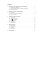
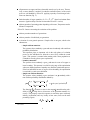
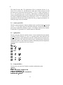
Chemical schemes are caracterised for each reaction (see Fig. 1) by a four real
numbers set. This allows to define the Arrhenuis law. Thus, a N-step chemical scheme
requires to fit 4N parameters.
1.2 The optimisation problem: cost function minimisation
The fit of scheme parameters can be seen as an optimisation problem. The aim is to
find the complete parameters set that let the corresponding scheme fits some predefined
reference ouputs. This kind of problem are often reduced to a minimisation one. The
idea is to minimise a cost function that represent the error or the distance between the
reference (or target) scheme’s ouputs and actual ones. The function to minimise is
presented in Sec. 2.2
The set of methods that solve the optimsation problems can be split into two main
types:
Gradient based methods
GA based methods
Gradient based methods are theoretically more efficient, and less CPU-time consuming. But global minimum research needs to use special “multiple seeding” technics,
since their main feature is to find local minima. The main drawback of these methods is their poor robustness face to the difficulty to sometimes evaluate the function to
minimise. In other word when the evaluation of the cost function fails, the classical
gradient methods are unable to evaluate function gradients and then to step beyond the
actual phase space position. Additionally these methods are not suitable when the cost
function shape is noisy or nearly chaotic.
On the other hand , GA methods handle very well unconverged function evaluations,
and are very robust in a general sense. Their main advantage resides in the way they
1
balance domain exploration (i.e research of new solutions) and optimum determination (precise location of the minimum). If this balance is well established, they
are quite unsensitive to inital conditions. Their main drawback is perhaps the number
of function evuluations face to efficient gradient methods. This evaluation cost and
general convergence may be grealty affected by GA ’s parmeters tunning.
1.3 GA basic principles
We introduce some basic considerations about GA . A GA is used as a minimiser.
Fig. 2 illustrates the direct relation between real life parameter (the genes) and our
problem. For our fit, we deal with a “monochromosmic animal” whose genes are the
scheme parameters. The biological vocab is naturaly used to describe GA . For our
problem we can make the following bijection:
a chromosom
a gene
a chemical scheme representation
a chemical scheme parameter
a population
a generation
an individual
one chemical scheme
a set of chemical schemes
a set of “breeded” schemes
parameter 1
Gene 2
parameter 2
Gene 3
parameter 3
Gene 4
=
parameter 4
Gene N
parameter N
Parameters set
Chromosome
Gene 1
1 chemical
scheme
1 individual
ADAPTATION
FITNESS
LEVEL
Figure 2: Animal genes vs scheme parameters set
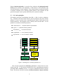
GA and more generally the evolutionary processes are centered onto an evolutionary loop (Fig. 3). This iterative procedure lets evolve a population generation by
generation under a selective pressure, i.e. keep alive individuals that fits our requirements. The selective critierion is usually called fitness function or objective function.
2
In our case, the fitness is kind of distance between the individual and a target point in
the search space. So be carreful not to do some confusion, small value of the fitness
function caracterises a well fitted individual. For this reason the fitness function term
is often replaced here, by cost function. New individulals are the offspring of a single
parent mutation or a cross-over between a couple of parents. The balance between domain exploration (Fig. 3 GENETIC OPERAORS block) and optimum determination
(Fig. 3 SELECTION block) is one of the key to success.
Strong selective pressure, by decrasing population diversity leads to premature
convergence i.e the minimum found is only local.
Weak selective pressure and too much mutation in population slow down optimum determination by wasting (CPU-) time in the evaluation of unfitted individuals (distant form the optimum). The search is uneffective.
The other main key to succes in GA performing, is the definition of the cost function. This definition determines directly the shape of the search space hyper-surface,
so may greatly influence the convergence rate of GA methods. Actually the cost function represents a norm of the distance that seprates the individual from a reference
point. This reference point is the target to reach. It must be realistic, i.e. reachable.
For example, it makes no sense to fit a 1-step scheme on S L for both lean and rich
operating points. See 2.2 for our cost function implemetentation.
FITNESS EVALUATION
Initial
population
of each individual
F ~ distance to target
GENETIC OPERATORS
Crossover/Mutation
CHILDREN
NEW
GENERATION
Evolution loop
population
SELECTION
FITNESS EVALUATION
Best live = F minimum
of each individual
F ~ distance to target
Figure 3: GA general principle
3
2
EP OR CK architecture and requirements
2.1 Mainframe
Random/Restart
1st Generation G1
Premix/Senkin system calls
Postprocess Chemkin binary files
Evaluate Fitness function
Loop over generations
Loop over population
Chemkin input files
GENOCOP III core
New generation
While G#<Gmax
Figure 4: EP OR CK general frame
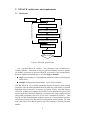
Fig. 4 presents EP OR CK structure. The evolutionary loop is initialised by a
scheme population. This initial set may be generated randomly respect to parameters bounds, or generated by previous EP OR CK run (restart) or pre-existing scheme.
Restart as random initialisation may be so called single or multiple:
single: only one scheme is generated then replicated to obtain an initial populationof clones.
multiple: each generated scheme differs a prori from its brothers.
Note that EP OR CK use a constant population (number of schemes) in the running
generation. Once the initial population enters the main loop, each scheme is evaluated
(population loop) by P REMIX (or S ENKIN in ignition version). Note that P REMIX
/EP OR CK coupling uses exchange files on disk, so avoid network file system (NFS)
that are much slower than local hard disks. Nevertheless this weak coupling does not
affect global performance since 95% of CPU-time is consumed by P REMIX . Then
the GA core take the popuplation as input to operate on it, selected genetic operators,
and selective pressure (some die some live but population remain constant). The main
loop is thus closed. Note that the process stops when reaching a specified generation
number.
4
2.2 Reference criteria and cost function
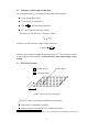
The selectable criteria Rk , are extracted from a laminar flame structure.
Sl , the laminar flame speed.
Tout , the burnt gas temperature.
δ0L
Tout Tin
max ∂T
∂x , the flame thermal thickness.
Ykout , the kth species outlet mass fraction.
The fitness2 or cost function F is defined as follows:
∑ αk Fk
F
k
where αk are the respective weights on the criterion set,
Fk
∑ αφ ln
φ
Rk
re f
Rk
where αφ are respective weights on operating points. R k are respective reference
or target values of selected criteria. Criteria selection, and weights settings are user
defined.
re f
2.3
EP OR CK features
Feasible domain
Penalty applied
Unfeasible domain
pa
ra
m
et
er
2
parameter 1
Figure 5: non-conex 2D search space
EP OR CK features concerning the definition of the problem:
multi-objective optimisation capability.
arbitrary numbers of parameters to fit. (multi-step schemes)
2 fitness
is the term used by GA community, in our case small fitness function
5
high scheme fitness
all parameters are upper and lower bounded, must be set by the user. Theoreticaly, a conex domain3 is needed. Nevertheless unfeasible part(s) of the search
space are well handled by EP OR CK applying a penalty to unconverged solutions cost function (Fig. 5).
limited number of target quantities (S l , Tout , δ0L , Ykout ) based on laminar flame
structure. (Ignition delays also but in an another EP OR CK version)
arbitrary number of operating points depending on Pressure, Temperature and/or
Mixture Composition.
EP OR CK features concerning the resolution of the problem:
arbitrary maximum number of generations
arbitrary number of individuals per generation
a selection of seven genetic operators. Simple refers to one gene, whole to the
chromosom:
– simple uniform mutation:
The operator selects randomly a gene and mute it randomly with a uniform
probability distribution.
This operators plays an important role in the early phases of evolution
process as the individuals are allowed to move freely within the search
space. This operator is essential when starting with a clone population as
it introduces novetly (phase space exploration).
– boundary mutation:
The operator selects randomly a gene g and mute it to one of its upper or
lower boundary. This operator is usefull in early stage of the optimisation
when user defined parmeters boundary may limit the optimisation process.
If the best individual has one of its gene at one boundary, the optimisation
is restricted by search space definition.
– simple non-uniform mutation:
The operator selects randomly a gene and mute it to g randomly with a
non-uniform probability distribution defined by :
g ∆ t upper bound
g
g
g ∆ t lower bound g or with equal probability The function ∆ t y returns a value in the range 0 y such that the probability of ∆ t y being close to 0 increases as the generation number t increases. This property causes this operator to search the space uniformly
initially (exploration) and very locally at later state (focus on the most
promising region).
t b
∆ t y
y
r
1 T
3 also
convex
6
where r is a random number from 0 1 , T is the maximum generation
number, and b is a parameter determining the degree of non-unformity..
The non-uniform operators are responsible of fine tunning capabilities of
the system.
– whole non-uniform mutation: This operator has the same behavior than
the simple non-uniform mutation. The mutation is applied on the whole
chromosom, i.e. each gene.
– simple arithmetical crossover: The operator selects randomly a gene location of two individuals g1 and g2 . There are two offsprings with the same
genom exept for the crossing gene location:
g1
g2
ag1 ag2 1 a g2
1 a g1
This operator uses a random value a 0 1 .
Arithmetical crossovers must be selected anyway. They have a stabilisation
effect on the evolutionary processes.
– whole arithmetical crossover: This operator has the same behavior than
the simple arithmetical crossover. The crossover is applied on the whole
chromosom, i.e. each gene.
– heuristic crossover: This operator is a unique crossover for the folowwing
reasons:
it uses values of the objective function in determining a direaction of
search.
it produces only one offspring, and may produce no offspring at all.
This operator behaves acording to the rule:
parent
parent
F I2
F I1
i.e individual 2 is better than 1.
parent
parent
child
I
r I1
I1
I2parent with r a random number from 0 1 .
If after some attemtps (varying r), the generated offspring is still not
feasible (i.e out of boundaries), then no offsprig is produced.
Its major responsabilities are fine local tuning and search in most promising direction.
adjustable selective pressure parameter. It is not recommended to modify it.
adjustable parameter for non-uniform mutation operators. It is not recommended
to modify it.
A restart functionality allows to restart an optimisation from the best individual
of a previous optimisation. It is also possible to restart from an entire generation.
See Sec. 3.4.
3
EP OR CK input files description
Here are the input files definition:
7
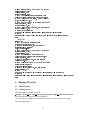
scheme.c No parser has been developped yet. Thus P REMIX format scheme
definition must be coded by user in C, then linked with EP OR CK binaries and
C HEMKIN libraries4 . See Sec. 3.1 for details.
input eporck.dat: contains information about operating points and also about
constraints’ number, type and value. Cost function weights are also defined
there. See Sec. 3.3 for details.
input genocop.dat: contains information about parameters’ number, range and
also population size maximum generation number and genetic operators selection. See Sec. 3.2 for details
premix.job: It is the P REMIX command files. If this file does not exit, it is
automatically generated. If premix.job is present, it must be consistant with
equil.job and input eporck.dat settings. i.e. same number of operating points,
and operating condition with respect to reference (constraint) value. See Sec.
3.5 for details.
equil.job: It is the E QUIL command files. It must be consistant with operating
conditions. It is used to generate runtime the premix.job file. See Sec. 3.5 for
details.
premix.sh is a sh script shell file that launch the transport interpreter and P RE MIX . See Sec. 3.6 for details.
equil.sh is a sh script shell file that launch the C HEMKIN interpreter and E QUIL
. See Sec. 3.6 for details.
restart.eporck optional file that contains chromosome(s) of individual(s) for
restart procedure. See Sec. 3.4 for details.
3.1 scheme.c file
X[]
real
of
parameter
to fit (indexed from 1).
is
the
vector
!"#$
% & ('!)
*&+,.-)/103254*+
&6
7 8:9 --;=< 87
>?&@A&BCD03E
&D4*+FE
G
7&8IH JK< 87
,J! 8 4.)J-L3E
,J! 8 &,3E
4& JM!&!N2OPE
QLR H ? 8 +,.-) *43E
4K/S4 *&+ TTU)6
G
4
)J-LTVW !&,-XYW+,,-LZLE
[
&+
G
4 chemkin.a,
chemkin public.a, surface chemkin.a
8
4
)J-LTV+,PW+,.-LZLE
[
+,-L *4 TD4
Y/S4.)J-L32, ' 6VE
4/+,,-L*4 TT HH 6
G
&!,&4F/
B
D
4 )+ 4! &&M4 J&XL2 4.)J-L)6XE
4+
/ ,&L6VE
3/ 6XE
[
! '),/+,,-L*46VE
7&888
8 @ ? ? QLR H ?M? 9 R.A)RB 88887
&TV ? H ? ? A $LE 4 !)& 4/+,,-L*4F2.+)21 ,&)6VE
&TV
B
@
$LE 4&!)&4F/+,.-L*4F2.)+))2S ,&)6XE
9 )E 4 !), 4/+,-L *432, +)L2S 6VE
&TV ? &TV ? @R.? LE 4&!, 4F/+.-) *432, )+L25&6VE
&TV@ DB @ B @B B LE 4&!,&4F/+,.-) *432.)+L2S&)6XE
9 )E 4 !), 4/+,-L *432, +)L2S 6VE
&TV ? &TV C? @ALRB LE 4&!,&4F/+,.-) *432. )+L2S&)6XE
7&8 C& J&.)D < 87
&TV@ !" $ #B T % @ B !B VLE 4&!,&4F/+,.-) *432. )+L25&,6XE
7 8 ' !
&&
'( ?&)
J 87
4 !)& 4/+,,-L*4F2. ? *
+Y 4 ,
-Y 4 $L2O'3./ ,U3250
0 /12L6V25UY U3250
0 /$2L6XE
7 8 ' !
&I+,&&,L.-)!)I44
&L+
@ =< 87
&TV Q&BC 9 7 @ LE 4 !)& 4/+,,-L*4F2. +)21 ,&)6VE
4 !)& 4/+,,-L*4F2. 4 7 L2 3
0 /4+2L6XE
7 8 B < 87
&TV Q&BC 9 7 B )E54 !)& 4/+,,-L*4F2. +)21,)6ZE
4 !)& 4/+,,-L*4F2. 4 7 L2 3
0 /52L6XE
7 8 CJ&
< 87
&TV@B !UY6 #B :T @ B LE 4 !), 4/+,-L *4F2.1 )+))2S ,&)6XE
7 8 ' !
&&
7) ?&J 87
4 !)& 4/+,,-L*4F2. ? *
+Y 4 ,
-Y 4 $L2O'3./ ,U3250
0 /$#2L6V25UY U3250
0 /982L6XE
7 8 ' !
&I+,&&,L.-)!)I44
&L+
@ B < 87
&TV Q&BC 9 7 @ B)E 4&!, 4F/+.-) *432, )+L25&6VE
4 !)& 4/+,,-L*4F2. 4 7 L2 3
0 /4-2L6XE
7 8 'J!N2 -&+
!& % !)+ ! ! :-J&&&J&, :L . &!,- 87
&T ; UFE
!&! T3
0 /4-2! E
&TV CBC 9 7 @ B)E54 !)& 4/+,,-L*4F2. +)21,)6ZE
4 !)& 4/+,,-L*4F2. 4 7 L2 !&! L6XE
7&8 B < 87
&TV Q&BC 9 7 B )E 4&!, 4F/+.-) *432, )+L25&6VE
4 !)& 4/+,,-L*4F2. 4 7 L2 3
0 /4<2L6XE
7&8 'J!L,32 - + ! % !L+
(! !M&:-J , J& :&. !)- 87
T ;UY$ #FE
!&! T3
0 /4<2! E
&TV CBC 9 7 B )E54 !)& 4/+,,-L*4F2. +)21,)6ZE
4 !)& 4/+,,-L*4F2. 4 7 L2 !&! L6XE
9 )E 4 !), 4/+,-L *432, +)L2S 6VE
&TV ? 4+/+.-) *4)6XE
[
9
3.2 input genocop.dat file
In the sample file each line is defined by a coment. Note the line numbering is only
for only added for convenience. Genetic operators (GOp) selection need some further
explainations:
Each interger refers to the number of individuals involved in a GOp. The selection
order is defined by the list of the GOp below. There are two important points to keep
in mind:
For crossover GOp, the number of individuals involed must be a multiple of 2
since 2 parents are needed to produce an offspring.
The sum of the number of individuals involed must be stricly inferior to the half
of the population size.
The selection order is:
1. simple uniform mutation
2. boundary mutation
3. simple non-uniform mutation
4. whole arithmetical crossover
5. simple arithmetical crossover
6. whole non-uniform mutation
7. heuristic crossover:
See Sec. 2.3 for a full definition of the GOp.
1
2
3
4
5
6
7
8
9
10
11
12
13
14
15
16
17
18
19
U
U
<
N
U
#UUUY U UN$<
+
V
8N
U
V
U
-
UY6#
<
#U
-
U
U
U
'&!&*
'&!&*
'&!&*
'&!&*
'&!&*
'&!&*
'&!&*
'!&*
U
U
UUUUN U
6 U
#
,UUUUY &
U 8
<Y
+#UUUN
6
N U
#N
U
*
J!&J,<
U
&
&
&
&
&
&
&
)J) +
)J!J-*
)J!J-*
)J!J-*
)J!J-*
)J!J-*
)J!J-*
)J!J-*
J!J-*
*.)J!&J,-
!&*
!&*
!&*
!&*
!&*
!&*
!&*
!&*
&
&
&
&
&
&
&
!&J+ -!
UY,U
+
&
% &! ++&! 44
U
-Z,-X+J
T U 7 -J-X +J&T"
10
U
2 II-L4;
)I!J&!L+ +
&
20
21
22
23
24
25
26
27
C? A CA Q H < -&)))I!J
& ,-)T UF2 +, &! J
& .-T"Z2
+,&& !&+.J!TF2 -&)) &! +.J!T+
J!J-L&!(4 !(;
4!&,-(-& J)
P2 II-L4;
8
.U
J!J-L&!(4 ! +- ) ! ++I % !Y2 II-)4;
+. J+
-!Y2 (+
3.3 input eporck.dat file
The sample file coments describe the file structure. Note the line numbering is added
only for convenience. This file is read via a parser. Any comment can be inserted.
The numerical values are only read after recognition of the folowing key-words (all
are finalised with :):
Constraints-number: Constraints-indexes: Constraints-weights:
OP-number:OP-weights:
Target-values:
Tere is no input order since the file is rewinded for each keyword.
1
2
3
4
5
6
7
8
9
10
11
12
13
14
15
16
17
18
19
20
21
22
23
24
25
888888888888888888888888888888888888888888888888
8
8
R A 9 A QB
CD? BC@ "
> 9 <
888888888888888888888888888888888888888888888888
;;;;;;;;;;;;;;;;;;;;;;;
8 @
Z+,!J , L+(+
.)
8
;;;;;;;;;;;;;;;;;;;;;;;
@+.!&J&&L+;
-! <
@+.!&J&&L+ ;& +< &8*@+.!J&&)+ ;'&
&)+< #3 U U*N U*N U
;;;;;;;;;;;;;;;;;;;;;;;;;;;;
8 B.!&J, &)+ +&
) 8
;;;;;;;;;;;;;;;;;;;;;;;;;;;;
B ;.-!P< +
B ;
'& L+$<
V
U
U
U
;;;;;;;;;;;;;;;;;;;;;;;;;;;;;;;;;;;;;;;;;;;;;;;;;;;;;;;;;;;;;;
8 C&4 !&
% J.+ < I
&, ! B 2 -& ! Z+,!J , 8
B V<
AJ! ;
B 3<
AJ! ;
B +N<
AJ! ;
;;;;;;;;;;;;;;;;;;;;;;;;;;;;;;;;;;;;;;;;;;;;;;;;;;;;;;;;;;;;;;
A
&*@B
*@B
# $<--UUU;U)
% J.+$< 3
$ --<UU!U+
+Y U -+8UU;U#
-N$- .<<UU;U
< U-UUU;U)
% J.+$< N
#8).UU!U+
N U +-UUU;U
N6).+UU;U
.-UU! UU
% J.+$< V
N +-UU!U+
Y4<UU;U
V U #<#UU;U)
11
26
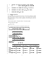
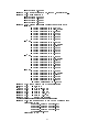
This input file means that: The optimisation will use 4 contraints wich are S L (selector #1),Tad (selector #2), the third species outlet mass fraction (selector #6) and
the fourth species outlet mass fraction (selector #7). The α φ weights coefficients (see
Sec. 2.2 ) are respectively 5.0 1.0 2.0 and 2.0 . Each scheme is evaluated with P REMIX
on three operating points (OP). An OP is defined by the fresh mixture temperature and
the mixture composition (defined in the equil.job file, see Sec. 3.5). The pressure is
assumed to have the the same value for all the OP. The α k weights are all equal to 1.0.
Finally the target values are tabulated.
3.4 restart.eporck file
This file is only needed when a single or multiple restart is specified in input genocop.dat
(see Sec. 3.2). For single restart, the information reduced to a unique line filled by the
genes (floats separated by tabulation or space). For multiple restart, the files contains
as much lines as a generation size. Each line defines an individual.
3.5 equil.job file
The user must only check the equil.job content. It must contatains the same number
of chained (CNTN) solutions (ie. same # of operating points) than declared in the
input eporck.dat file. At the initilisation, equil.job is read to generate the premix commad file: premix.job. This, taking into acount, pressure, inlet temperature, and mixture
composition in order to setup temperature profiles, and chained premixed computation.
Note that mixture composition unit is mole fraction.
equil.job:
C? V U
A? +UY
U U
C ? @
@
C ? @
B C ? @
A? A .<U U
@ A ? 9
C ? @
@
C ? @
B C ? @
@ A ? 9
C ? @
@
C ? @
B C ? @
? 9
UY$#UU
N UUU
-Y$ #U
UY9<UU
N UUU
-Y$ #U
1.UU
N UUU
-Y$#U
3.6 Script shell files
The user must only check the Chemkin executables and databases paths.
equil.sh:
7 L, 7 +
J M@,-), &&J )+
@ T 7 J 7 ,.-L,+8 7 ! .-Z +,-L J,-LF2 9 B&BA&B 9 R,Q
+,-LT&! .-X
1+,.-)
12
'J
.-) )J & 4 ! M
&&
,-L T 7 % 7 )
,.-)&T.- &
,.-L&, &T,,- J+
J (!-);)J-X &JJ )J+
(4
,.-&JT 7 J 7 ,.-L, +8 7 J J 7 !- J
? : .--J. 4:)J,-)32 9 BBA&B 9 R.Q
:&, T :LN 'J
:
& JM& 4M!(M &
:L
&T 7 % 7 : T :L3 ? : + .&M4I)J-LF2 9 B B
A B 9 R,Q : T :L3 ,.-L, ,& !&!&&!
@ 7 ,,- ;& +.-)
; ,.-L
&
;& ,-& ; .-&J
? :
@ 7 :L
;& :L&&*
; :
&,
;
: ; ,.-L&,
7 premix.sh:
L, 7 +
J M@,-), &&J )+
@ T 7 J 7 ,.-L,+8 7 ! .-Z +,-L J,-LF2 9 B&BA&B 9 R,Q
+,-LT&! .-X
1+,.-)
,.-L&, &T,,- J+
'J
!J
)J & 4 ! M
&&
!J. T 7 % 7 )
!&J
&T!J
" &
J (!J.Z+!M&JJ )J+
4
!&J
&&JT 7 J 7 ,.-L, +8 7 J J 7 !&J.O&J
!&J
&, &T!J. J+
&! .-Z ,--LJ
432 9 B B&
A B 9 R.Q T&!&,-X
'J
M !&.-Z& )J & 4M!(M
&&
!&,-X T 7 % 7 )
&! .-Z &T&! .-Z ! .-Z +
)
D4F2 9 B &B&
A B 9 R,Q +J % ,&T)+J % N L,
!&J
@ 7 !J. ; !&J
&
; !J.&J,
;& ,.- ,
&! .-Z
@ 7 &!&,-X
;&
; !&,-X *
;
+J % L,
,;
;
!J.) ,
.-L&
,;
!J
&
4 Running EP OR CK
4.1 Run check list
4.2 Getting started
The command line to launch EP OR CK :
eporck V1.6 input genocop.dat genocop.out input eporck.dat eporck.out
prompt
Note that these file names can be user (re)defined.
The user can pause/continue or stop EP OR CK before the normal program exit, using
the folwing procedures:
13
PAUSE: Simply create a file named PAUSE EPORCK in the running directory. This easily done with the command: touch PAUSE EPORCK
Note the program effectively pauses when the evaluation of the current generation is completed. So it may not be instantaneous. Check if eventually an old
GO EPORCK file is in the directory. If any, delete it before. If you do not delete
it, the program pauses but restart within a short time.
CONTINUE: To continue the run after a pause:
– Delete the PAUSE EPORCK file.
– Create a file named GO EPORCK. The program will restart within a
minute.
STOP Simply create a file named STOP EPORCK in the running directory.
This easily done with the command: touch STOP EPORCK
This feature allows to stop properly EP OR CK before the maximum number of
generations, in order to complete all output files properly.
4.3 Output files
The genocop.out file (see Sec. 4.2) contains convergence information. Each time a
new individual is the best, a line is appended. It contains generation number and cost
function
value.
Q! ,
# V<6N<9UUU+
?:)J&
+ <
R :)J + <
9 ,-J ,Z+ <
#N UU
T 0"
T
#3 UU
#UUUY UU
T 0
T
UUUUY UU
UN9 U
T 0+
T
3 UU
UN9 U
T 0
T
3 UU
8N UU
T 0#
T
#N UU
#UUUY UU
T 08
T
UUUUN UU
+N UU
T 0 T
N UU
#UUUY UU
T 0<
T
UUUUN UU
UN UU
T 0 T
+N UU
UN UU
T 0 .U T
+N UU
A&+. J+:- !
< - !D4D!J&!)+
< U - !D4M !&J)+ < .UU
J
+ < U
J!J-L !
< 8
J!J-L !
< UY1.UUUUU
88888 R IC ? A C A 88888 R .
R H ? B&R A R LR,ALR H& B H ALRBP
)M>&J.
!J
!J
<
V6 -+# !J
<
UN$ +#+-+8+
!J
<
+
UN6 <+--++
!J
<
<
UN6 <).#8 .
!J
<
UN6 <) #U +
!J
<
.U
UN6 #U .<+<
? CB@ % C )R 32 ? 9 ?&
C ?C C ? ? A ? CB@ %IAB B ? 9 2 A ? &L, B*? B
C@$ R. CLR. 9 R,C?&@A&BC
? CB@ %IA LR MABIC? B>? ?*? BC@ ?QB
C ?
? CB@ % C )R 32 B ? 9 9 ?
C ?CMC? ? AP
!J
<
)
UN <#- #
!J
<
+U
UN < .-U 14
!J
<
+ UN 8".8-8
!J
<
+#
UN 8 U<8U
!J
<
+
UN.<<< !J
<
"
UN.-<<88
!J
<
UN.8#8
!J
<
+
UN ++8
!J
<
UN +<-8
!J
<
#)
UN +<
!J
<
#UN + 8U
!J
<
8U
UN -" !J
<
8UN 88 .8
!J
<
<
UN 8
!J
<
<+
UN 8) -<
!J
<
<8
UN 8).U !J
<
<<
UN # -
!J
<
UN # U
!J
<
UN # 8+#
!J
<
<
UN # #-
!J
<
,UU
UN # ##+
&+. +
) 'J+ 4&DJ !J)
,UU
&+. +
)D4 <
0 /.2=<
0
<N$+ U+U
0 / 2=<
0
<#-Y$ #-8#8#
0 / +2=<
0
V U U 8-U 0 / 2=<
0
V6 #8#
U <0 / #2=<
0
N$ <#88-U
0 / 82=<
0
.8#-N9 +# #8#U
0 / -2=<
0
-N6 #-<
0 / <2=<
0
+<#<Y9 -8) - .<-#
0 / 2=<
0
V
+) <#+
0 /1,U 2 <
0
UN U +<#+
? B
C@ %(@!! +&,& +,.-L 4I' !
A&JI! )-) < #).<# +&
)+
/+
.&) % J.(T UN
# ##+)6
/ !&,-XYW+,,-L6
The eporck.out file contains a run summary and information about each individual
evaluation.
used for debuging.
? B
C@ > Essentially
9<%: !&,-XY D4 + +.)+ 2 !J) !&,-XY 88888888888888888888888888888888888888888888
8888888888888 ? BC@ ? RB 888888888888888
8 ? % &
)J!; !&&!&I4 !M
8
8 B.&-X+J)
4D@,-XJ LM+,.-L+ 8
8 >?C RB > V$ <U
8
88888888888888888888888888888888888888888888
? B
C@ > 9 <% C C P<
? B
C@ > 9 <%- !M4 Z+,!J , L+< ? B
C@ > 9 <%- !M4D!&J)I&L+ / -X
&!&M,-&+.)
X6 < ? B
C@ > 9 <% RD4 !&,-X & +.&MJ+ &J! .!).&!J3<
; @!).&!)
< M+
; @!).&!)
< +
; @!).&!)
< + +
; @!).&!)
< 8 +
; @!).&!)
< - +
; @!).&!)
< < +
; @!).&!)
< +
? B
C@ > 9 <% C&++I'&
L+(+- *
N UUUUUU 2 !-LJ Y
? B
C@ > 9 <% C&++
+ '&
& <
; /12 < UY9 +-+
; /12 < UY9 +-+
; /$2 < UY
.+-+ ; /9+2 < UY U +<+
; /42 < UY U +<+
; /$#2 < UY U +<+
; /982 < UY$ +).
U +#
15
< UY U+<+
'&)+ +- & 3 UUUUUU 2 !
-J&,& B + '
L+ <
; /12 < UY$ ++++++
; /$2 < UY
.8888; /9+2 < UY
.8888; /42 < UY$ ++++++
? B
C@ > 9<%IA&J! (!&+
Z++/W
!J,& &, MT B 6$<
;MB "
; A&J! ! ++( TDUY$#<--UU
; A&J! ! ++((T --Y9 <UUU
; A&J! ! ++(+ TDUY UU
U #<U
; A&J! ! ++(MTDUY UUU
U +)
; A&J! ! ++(#(TDUY U --) <<
; A&J! ! ++(8 TDUY U 8+<U #
; A&J! ! ++(- TDUY UUUU
U ;MB ; A&J! ! ++( TDUY9 <
U -UU
; A&J! ! ++((T #8Y U -8
; A&J! ! ++(+ TDUY UU
U ; A&J! ! ++(MTDUY UU
U U ; A&J! ! ++(#(TDUY U +
; A&J! ! ++(8 TDUY U -#-++
; A&J! ! ++(- TDUY UUUU ;MB +
; A&J! ! ++( T 1
- UU
; A&J! ! ++((,
T ) +Y9 8#
; A&J! ! ++(+ TDUY UU
U +-+
; A&J! ! ++(MTDUY UU
U #U
; A&J! ! ++(#(TDUY1
.U #<#U
; A&J! ! ++(8 TDUY U <-#U
; A&J! ! ++(- TDUY UUU
U ;MB ; A&J! ! ++( T 4 U +8UU
; A&J! ! ++((,
T 8Y9 +U ; A&J! ! ++(+ TDUY UU
U ++; A&J! ! ++(MTDUY U
U +) ; A&J! ! ++(#(TDUY1
-U <U
; A&J! ! ++(8 TDUY U <)
;(AJ! !&+
Z+
-MTDUN UUU #
? B
C@ > 9 <%(@
& C? LR
0 4 J!&J,-L&!L+<
? B
C@ > 9 <%
;
A T #
? B
C@ > 9 <%
; 0 ACD
T ;)V6 #UD? B
C@ > 9 <%
; 0
? 9 T Y UUD? B
C@ > 9 <%
; 0 @
? MT UN UUD? B
C@ > 9 <%
;(AQLR.0 T
,
U -+N U ? B
C@ > 9 <%
; R.0 T
UN6 UD? B
C@ > 9 <%
? 9 BQ C C 88888888888888888888888888888888888888888888
? B
C@ > 9 <% C & ? A < Q! ,
# V6< N9< U UU+
@+.!J&&(DUY<
B < UIC&TUY U #)- C
&T UY$ #<-B 1< C&TUY U 88-<8 C
&T UY9 <U B $< C&TUY U < ,U .< C
&"
T 1 -
B 9< +IC&TUY U +-+ C
&"
T 4 U +8
Q
++ / U 2T N6 # UU #
@+.!J&&( <
?
B
C@ >
? B
C@ >
;
9<%
9<%
B
/9-2
16
B
< UIC&T -8Y4+ C
&T" --N$<
<1 C&T <Y # C
&T" #8N
B <$ C&T) +Y98- C
&T) +N$B <9+IC&T #-Y4# C
&T8N9
Q
++ /12TUY UU 8#
@+.!J&&(,N<
B < UIC&TUY UU <<-8+ C& T UN UUU#<U
B 1< C&TUY UU -+U +#< C& T UN UUU",U+
B $< C&TUY UU 8 U 8+- C& T UN UUU +-+#
B 9< +IC&TUY UU #<#< C& T UN UUU ++8<#
Q
++ /$2T N$ <U <@+.!J&&(*+Y<
B < UIC&T N$ <8< ;U # C
& T +Y U -+8 ;U #
B 1< C&TUY UU)
U -) < .8 C
& TUY UUU U +B $< C&TUY UUU <88+ C
& TUY UUU <
B 9< +IC&TUY UU +) +) - C& T UN UU + Q
++ /9+2TUY < @+.!J&&( <
B < UIC&TUY U -# +<< C
&T UY U -- <<
B 1< C&TUY U U -<+ C
&T UY U ) +
B $< C&TUY1 .U U - C& T UN ,U #<#
B 9< +IC&TUY1 #UU C& T UN -U <
Q
++ /42TUY )
U -) <<<
@+.!J&&(,#N<
B < UIC&TUY U 8#++< C
&T UY U 8+<U #
B 1< C&TUY U -8-8 C
&T UY U -#-++
B $< C&TUY U <) ## C
&T UY U <-#
B 9< +IC&TUY1 .U ,UU + C& T UN U < Q
++ /$#2TUY )
U -<+
@+.!J&&(*8Y<
B < UIC&TUY UUU +U 88U < C
& T +Y9 <8< ;U 8
B 1< C&TUY UUU +<-+ C
& T 4 U ;U #
B $< C&TUY UUU ".8U - C
& T 9 <<<- ;U #
B 9< +IC&TUY UUU +-< 8# C
& TUY UU)
U .#+#
!J
U
Q
++
T V6 -+#+
B
The evaluation.log file contains the evalutation history. For each generation, an
individual evaluation is summarised on a line by its:
generation number
the cost function evaluation
genotype i.e the gene (parameter) sequence.
The best.scheme file is a C HEMKIN scheme format file updated at each improvement.
It
? H describes
??A the best scheme at the moment.
B
? 9
?&@R.? @ B @B
? 9
C ? @ALRB @ ! 6 #B
QB
C 9 7 @ QB
C 9 7 B
@ B ! UN6 #B QB
C 9 7 @B
QB
C 9 7 B
@
@ BB&B
T% @ B&!
1
.U<88
6 #8
U TD@ B
UUUUUU
UY6 #UUUUU
B
7
7
7
N9--<<#?! <
UN U
<) $ <
-Y9 .-?!U
UN U
. .U8Y
7
17
U
B (T%&B
QB
C 9 7 $<U+<- 7
QB
C 9 7 B UY$8UU 7
? 9
!
U-<<?!U
UN$<<
8U8+N6#
The premix.scheme file is a C HEMKIN scheme format file updated at the end of
the run. It describes the best scheme of all.
4.4 Specific tools
These tools aim to facilitate the generation of constraints target values. The 1D laminar
flames are computed with a complex chemical mechanism such as the GRI-Mech 5 for
methane, or natural gas. The user must be able to extract reference quantities such as:
Sl , Tout , δ0L Ykout . Two essential tools help to extract these values from binary P REMIX
V3.x solution file:
makeref V1X: This fortran tool reads the binary P REMIX file, and then edit an
ASCII column file. It contains:
– one line per operating point i.e for each equivalence ratio.
– each line composed by one column per quantiy. The quanties order is: φ,
Sl , Tout , δ0L and Ykout . For outlet species mass fractions, the order is the one
declared in the premix scheme file.
There is a default input file called makeref.choices composed of three lines:
1
2
3
4
+J % Y L,
UY4
$ #
UY1 C ? LR
0 L,J!; + ) 4:)J,-)
4
!L+,D: % JLI!&J , J+.M :L % J
I!J) &,&
: % JL:!J) +,&
extcol: This script tool extracts selected columns of an ASCII file ignoring lines
begining with the # character.
Example: The user wants to extract columns 1, 2, 17, and 5 from a file called
“reference.dat” to a file called ”myrun ref.dat”. He types in an UNIX shell window: extcol reference.dat 1 2 17 5 myrun ref.dat
pre2slt2:
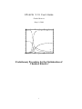
A fortran tool that postprocess P REMIX solution and plot S l φ and
Tout φ in an xmgr window.
pre2yk2: A fortran tool that postprocess P REMIX solution and plot Ykout in an
xmgr window.
5 http:www.me.berkeley.edugri
mech
18
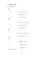
5 Problem sample
2-3 step-scheme ideas:
1.
CH4 O2
CO H2 H2 O
2.
CO H2O
CO2 H2
3.
2H2 O2
1.
CH4 2O2
CO 2OH H2 O
2.
CO H2O
3.
H2 2OH
1.
CH4 2O2
2.
CO 2OH
1.
CH4 3
O2
2
2.
N2 1
O2
2
19
2H2 O
H2 O CO2
1
O2
2
Jones & Lindstedt like:
CO2 H2
CO 2OH H2 O
CO 3.
2H2 O
CO 2H2 O
CO2
NO
1.
Cn H2n
2
n
O2
2
2.
nCO 1
O2
2
H2 3.
CO H2 O
n 1 H2
H2 O
CO2 H2
4-step with Zeldovich simplified mechanism #1:
1.
CH4 3
O2
2
CO 2H2 O
CO O2
CO2 O
N2 O
NO N
N O2
NO O
2.
3.
4.
4-step with Zeldovich simplified mechanism #2a:
1.
CH4 5
O2
2
2.
CO 4OH
CO 4OH
CO2 2H2 O O
N2 O
NO N
N O2
NO O
3.
4.
4-step with Zeldovich simplified mechanism #2b:
1.
CH4 3O2
CO 4OH O
CO 2OH
CO2 H2 O
N2 O
NO N
N O2
NO O
2.
3.
4.
20