Download CONCEPT-II Version 12.0 User's Manual

•
CONCEPT-II Version 12.0
User’s Manual
Institut für
Theoretische Elektrotechnik
www.tet.tuhh.de
Dr.-Ing. Heinz-D. Brüns, Dipl.-Ing. Angela Freiberg
Copyright: Institut für Theoretische Elektrotechnik, 2014
- Nov. 2014 -
2
Manual of the Program System
1 General description .......................................................................................................................... 4
1.1 Supported platforms and the code capabilities ........................................................................ 4
1.2 Possible excitations .................................................................................................................. 4
1.3 Post processing ........................................................................................................................ 5
1.4 Installation ............................................................................................................................... 5
1.5 Covered frequency interval, limits ........................................................................................... 5
1.6 Discretization ........................................................................................................................... 6
1.6.1 Rules for discretizing structures ....................................................................................... 7
1.7 Three essential steps for solving a problem ........................................................................... 12
1.8 Some file names ..................................................................................................................... 13
1.9 Performing a typical simulation ............................................................................................. 14
1.9.1 Overview ........................................................................................................................ 19
1.9.1.1 Icons of the tool bar ................................................................................................ 20
1.9.2 The simulation project tree ............................................................................................. 22
1.9.2.1 Handling of the simulation project tree .................................................................. 23
1.9.2.2 Dielectric bodies ..................................................................................................... 24
1.9.2.3 Wires ....................................................................................................................... 28
1.9.2.4 Frequency sampling ............................................................................................... 32
1.9.2.5 Voltage generators .................................................................................................. 34
1.9.2.6 Ports ........................................................................................................................ 35
1.9.2.7 Plane wave field ..................................................................................................... 37
1.9.2.8 Impressed wire current ........................................................................................... 39
1.9.2.9 Solvers .................................................................................................................... 40
1.9.2.10 Precision of the numerical solution ...................................................................... 41
1.9.3 Post processing tools ...................................................................................................... 43
2 Example: Top-loaded wire antenna on a table structure ................................................................ 52
The handling of the GUI shall be demonstrated by a simple example. ...................................... 52
2.1.1 The discretization of the surface part ............................................................................. 54
2.1.2 Post processing ............................................................................................................... 59
2.1.2.1 Representation of the current distribution .............................................................. 60
2.1.2.2 Representation of 2D electromagnetic field distributions ...................................... 61
2.1.2.3 EM fields along straight paths or at arbitrary locations in space ........................... 63
2.1.2.4 Creating 2D radiation diagrams ............................................................................. 66
2.1.2.5 Creating 3D radiation diagrams ............................................................................. 68
2.1.2.6 Creating Smith diagrams ........................................................................................ 71
3 Important topics ............................................................................................................................. 71
3.1 Dielectric bodies, types of surfaces ....................................................................................... 71
3.1.1 Bodies of high conducting material ............................................................................... 72
3.1.2 Field-coupling through apertures ................................................................................... 73
3.1.3 Multi-dielectric block with symmetry ............................................................................ 74
3.1.4 More examples ............................................................................................................... 75
3.1.5 Wires in dielectric bodies, wire junctions ...................................................................... 77
3.1.6 Layers on bodies ............................................................................................................ 78
3.1.6.1 Example of a cylinder with a lossy wall of high relative permeability .................. 80
3.2 N-ports, S-parameters ............................................................................................................ 81
3.2.1 Files ................................................................................................................................ 83
3.2.2 Computation of S-parameters ........................................................................................ 85
3.2.3 EM fields when port excitations are modified ............................................................... 86
CONCEPT-II, User's Manual
3
3.3 RCS ........................................................................................................................................ 92
3.4 Computation of line integral of E and H ................................................................................ 94
3.4.1 Example: Line integral to measure the surface current .................................................. 96
3.5 Integrating the Poynting vector on a triangulated surface ..................................................... 98
3.5.1 Example: Loaded circular wire loop .............................................................................. 99
3.6 Discretizing structures ......................................................................................................... 101
3.6.1 Spheres, plates, cones, cylinders etc. ........................................................................... 102
3.6.2 Treatment of wires ........................................................................................................ 110
3.6.3 Generating triangular and quadrangular plates ............................................................ 112
3.6.4 Using the boundary tool ............................................................................................... 116
3.6.5 Effective discretization of wire contour models .......................................................... 119
3.6.6 Using the point option for discretizing ........................................................................ 121
3.6.7 Joining surface parts with unwanted gaps .................................................................... 124
3.7 Importing and exporting ...................................................................................................... 126
3.7.1 Converting STL data into surface patch format ........................................................... 126
3.7.2 Converting the wire format into the .geo format of gmsh ........................................... 129
3.7.3 Using the CONCEPT-II patch format for mesh generation in gmsh ........................... 131
3.7.4 Visualizing field and current distributions by means of gmsh ..................................... 133
3.8 Time domain system responses by an IFT ........................................................................... 134
3.8.1 The necessary steps in short ......................................................................................... 134
3.8.2 Key points for performing an IFT ................................................................................ 137
3.8.3 Frequency sampling for an IFT .................................................................................... 146
3.8.4 Special aspects: Impressed currents and lightning currents ......................................... 148
3.9 Using CONCEPT-II for parallel computation ..................................................................... 151
3.9.1 Linux ............................................................................................................................ 151
3.9.2 Windows ....................................................................................................................... 152
3.10 Format of surface patch files and wire files ....................................................................... 152
3.11 Arrow scaling, xtrans, ytrans ............................................................................................. 154
3.12 Backup of project directories ............................................................................................. 155
3.13 Known problems ................................................................................................................ 155
4 Theoretical background (method of moments, EFIE, MFIE) ..................................................... 156
CONCEPT-II, User's Manual
1 General description
4
1 General description
CONCEPT-II is under development at the Institut für Theoretische Elektrotechnik
Theory at the Technische Universität Hamburg-Harburg. It is a program package for
the numerical computation of electromagnetic radiation and scattering problems in
the frequency domain. The code is based on the Method of Moments (MoM) for
solving the electric integral equation (EFIE) in the case of metal structures and a
set of coupled integral equations in the case of (lossy) dielectric bodies, see Sec.
4 . It is designed for the computation of currents, voltages and fields, which result
from the electromagnetic excitation of wire or surface structures. The application of
the package is limited to linear materials which have to be homogeneous and
isotropic in sections.
1.1 Supported platforms and the code capabilities
PC running under Linux and Windows.
The code capabilities include the treatment of:
●
●
●
●
●
●
●
●
●
●
●
●
Lumped circuit elements at any location on wires and metallic surfaces
Arbitrary metallic surfaces, which are simulated by the electric field integral
equation (EFIE, single-layer current distribution)
Surface impedance
Thin lossy sheets on ideally conducting surfaces (not yet described in this
manual, thin sheet approximation, TSA)
Anisotropic layer material (CFC, not yet described in this manual, currently
only for surface structures)
Lossy dielectric bodies modeled by double-layers of electric currents
Bodies covered by thin layers of finite conductivity to analyze shielding
problems for example
Structures in free space and over an ideally conducting ground plane
Various magnetic symmetry planes
Parallel LU decomposition
Parallel MLFMA
ACA
1.2 Possible excitations
●
●
●
Voltage generators and power generators (ports) on wires, edge generators
on metallic surfaces
Impressed line current source (current generator)
Plane-wave fields of arbitrary polarization and direction of incidence
CONCEPT-II, User's Manual
1.3 Post processing
5
1.3 Post processing
Once the matrix equation resulting from the application of the MoM has been set up
and solved, the current distribution is known. Based on this current distribution
system responses such as electromagnetic fields at arbitrary positions in space can
be can be computed and displayed.
Most important features:
●
●
●
●
●
●
●
3D and 2D radiation diagrams
Monostatic RCS
Current distributions on surfaces and wires
System responses (I,U,E,H) as a function of frequency
Time domain system responses by an inverse Fourier transform (IFT)
2D and 1D field distributions
Electromagnetic fields at arbitrary observation points...
For a successful application of the code the user should be familiar with the basic
theory. A short outline is given in Section 4.
1.4 Installation
A document available on the CONCEPT-II download web page contains details
about the installation of the package.
1.5 Covered frequency interval, limits
The conventional MoM provides a dense complex system matrix. This requires
O(N2) to store the matrix elements and O(N3) to solve the equation system by LU
decomposition for example, with N as the number of basis functions used to
approximate the physical current distribution. The investigation of electrically large
structures may become uneconomic using the LU decomposition, at first depending
on the available hardware resources. The state-of-the-art technique for large hight
frequency problems is the multilevel fast multipole algorithm (MLFMA) which is
available as a solver.
Each common edge between two neighboring surface elements (patches, triangles
or quadrangles) leads to one unknown in the case of the EFIE (metal, single-layer
current distribution) or to two unknowns in the case of a dielectric body (doublelayer current distribution), respectively. The total number of unknowns N depends
on the electrical size and on the geometrical complexity (“overall grid”) of the
structure under investigation.
An important rule of thumb is that 8....10 segments or patches per wavelength are
necessary on electrically large structure parts, leading to an increasing number of
unknowns at higher frequencies.
The core memory to hold the system matrix can be determined as follows:
CONCEPT-II, User's Manual
1.5 Covered frequency interval, limits
N⋅N∗16/ 1024
3
6
(LU decomposition)
Hence an important limit of the problem size to be treated is determined by the
available core memory (RAM). Note that CONCEPT-II does not include an out-ofcore solver anymore starting with version 12.0. The amount of in-core memory
used by CONCEPT-II should stay smaller (70%,..,80%) than the memory being
physically available . Additional memory is necessary, depending on the structure
under investigation.
Examples:
Number of unknowns N=1000 (small problem) → 0.0149 Gbyte
Number of unknowns N=10.000 (medium sized problem) → Memory necessary to
hold the system matrix: 1.49 GByte
Number of unknowns N=100.000 (large problem) → 149 GByte
The smallest frequency which is possible is in the range a 1,...,10 kHz depending
on the geometrical size and the type of integral equation used. Metallic structures
(EFIE) with a typical dimension in the range of 1 meter or larger can be computed
even at lower frequencies.
Transient system responses can be gained by computing an appropriate number of
samples in the frequency domain and performing a successive inverse Fourier
transform (Sec. 3.8).
1.6 Discretization
CONCEPT-II includes powerful tools for creating surface patch meshes
(discretization). Surface patch meshes may comprise planar triangles and/or (nonplanar) quadrangles.
Nevertheless, for sophisticated meshing purposes external tools such as gmsh
(http://geuz.org/gmsh) or salome (http://www.salome-platform.org) could be very
helpful. Salome includes various open source licenses and Gmsh is distributed
under the terms of the GPL. Both are able to read CAD data formats such as IGES
or STEP and are able to convert the corresponding surfaces into discretized
structures of STL format, which in turn can be read by CONCEPT-II. How to use
gmsh in conjunction with CONCEPT-II is outlined in Sec. 3.7.
Tip
Formats like IGES (.iges files) or STEP (.step files) can
easily be turned into the grids by gmsh (.msh files) and from
this into the CONCEPT-II surface patch data format, see
Section 3.10.
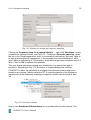
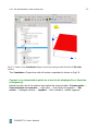
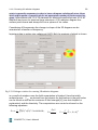
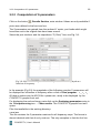
For usage of the CONCEPT-II import/export tool click on Misc → Import/export
→ the corresponding dialog opens as depicted below.
CONCEPT-II, User's Manual
7
1.6 Discretization
Fig 1.1: Tool for converting various files formats
The available features include:
●
●
Conversion of STL data into the CONCEPT-II surface patch format.
Conversion of the output of the gmsh tool into the CONCEPT-II surface patch
data format.
Note: .msh files can be directly loaded into the simulation. The data is automatically
converted into the CONCEPT-II surface patch format. The corresponding files have
the suffix .surf .
1.6.1 Rules for discretizing structures
Important
A proper mesh is essential for the success and the
convergence of the numerical computation.
It not sufficient that the structure under consideration is described 'somehow' by a
surface patch pattern giving the right three-dimensional impression. Very important
is a proper structure discretization related to the electromagnetic requirements. In
this context we have to distinguish between electrically large and electrically small
objects and structure parts, respectively.
Generally a wire is characterized by a straight line that extends between the start
coordinates (Xstart, Ystart, Zstart) and the end coordinates (Xend, Yend, Zend).
This is also the current reference direction. Between both ends a wire is subdivided
into a number of segments. In the following it can be assumed that the number of
wire segments corresponds to the number basis functions on a wire.
In general a surface is subdivided into a number of surface elements (“patches”).
Triangles should be preferred.
CONCEPT-II, User's Manual
8
1.6.1 Rules for discretizing structures
●
●
●
Wires and surfaces which are large in terms of the wavelength (electrically
large) have to be discretized assuming 8,...,10 patches or wire segments
per wavelength at least.
The minimum number of basis functions should be three on electrically
short wires, especially on wire grids. The minimum number of basis
functions for short monopole antennas should be 6...8; 12...16 are
sufficient on electrically small dipole antennas.
No simple rule can be given for the discretization of electrically small
structures. For parts which are small in terms of wavelength it may be
important that geometrical details are modeled in a sufficient manner.
Example: sphere with 1 m in diameter, f= 1 MHz → λ=300 m. Applying
the high frequency rule we would have a typical patch size of 10 m
which is not possible, of course. For a rough model of the sphere we
have to apply 8,..,10 patches around the circumference to keep the
outline of the sphere properly.
In the low frequency region the user should answer the following question:
“How many patches/wire elements are necessary to get a good
approximation of the charge distribution under the assumption that only
constant charge blocks are available on each triangle, quadrangle or wire
segment”.
In general physical charge distributions are numerically approximated by a
step functions. It is well known that we have a rapid increase of the surface
charge distribution for example when approaching a sharp edge. Thus, if the
electric field strength is of interest close to such an edge an appropriate grid
refinement has to be introduced.
●
For wires the well-known thin wire assumptions have to be fulfilled:
L ≫ a, a ≪ λ
with L as the wire length, a as the radius and
λ as the wavelength.
Wires should be much longer than thick. Parallel wires should not get too
close to each other. The radius of a wire should stay much smaller than the
wavelength.
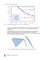
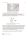
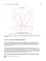
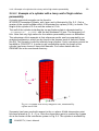
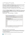
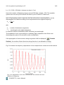
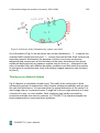
In Fig. 1.2 can be seen how the characteristic impedance of a single wire
line is behaving, when approaching the ground. The analytical solution
refers to the red curve. The blue curves indicates the behavior of the
characteristic impedance assuming a simple current filament on the wire
axis. Starting at approximately r/h=0.3 (radius over height) the error gets
more and more pronounced, even when assuming an ideal ground. One
can imagine that an image wire is running at -h.
Hence for an accurate solution the axial distance of two (or more) wires in
parallel should not be closer than approximately 4 times the largest radius.
CONCEPT-II, User's Manual
1.6.1 Rules for discretizing structures
9
Fig 1.2: Characteristic impedance of a wire over a ground plane
●
●
The ratio of the segment lengths of wires that are connected to each other
should not exceed 10,...,15. Parallel wires should be discretized in the
same way.
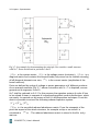
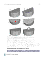
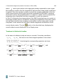
Tiny patches should not be attached to much larger ones. Patches with a
big ratio of edge lengths should be avoided, see Fig 1.3 and Fig 1.5
demonstrating bad examples. The same statement holds for triangles where
1 or 2 vertices are forming small angles.
Fig 1.3: Examples of surface patch combinations that should be avoided
CONCEPT-II, User's Manual
1.6.1 Rules for discretizing structures
10
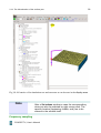
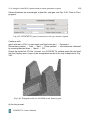
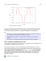
Fig 1.4: Example of a partly bad mesh. The discretization of this vase is good except for
the bottom. Here we see only individual triangles extending between the rim and the
center of the bottom disk - at least 5 to 6 were necessary (also for very low frequencies)!
Here the highest frequency possible is determined by the long edges at the largest
diameter of the vase. Hence the grid at the bottom is insufficient for both high and for
low frequencies. From an electric point of view the bottom discretization makes
absolutely no sense.
●
Wires running parallel over a discretized ground plate, the typical size of the
patches underneath the wire should be smaller then two times the height of
the wire (perpendicular to the wire axis at least). Otherwise the
characteristic impedance of the wire cannot be captured. Note that C' and L'
are not input quantities – they are modeled by the sources on the local
grid.In Fig 1.4 the bottom of the vase has been discretized according to
pure visual aspects – this an error frequently encountered.
CONCEPT-II, User's Manual
1.6.1 Rules for discretizing structures
Fig 1.5: Example of a bad grid:
We see an inhomogeneous mesh which cannot be accepted including
•
tiny triangles close to very large ones
•
Triangles with the shape of needles (two corner close to 90 degrees or one
corner close to 180 degrees)
•
An erroneous quadrangle (corner angle larger then 180 degree), quadrangles
with one corner angle close to 180 degrees or a quadrangle with one corner
angle of only a few degrees.
Note
●
A mesh has to be generated always based on
electromagnetic requirements not on visual aspects.
Some simple examples: An electrically small disk with a wire antenna
mounted in its center should have at least 5...6 patches between the center
and the outer boundary. An isolated square plate should have at least 6
patches along each edge, even in case of a large wavelength.
Grid errors may be detected by a tool which can be found under
CAD tools → CAD tools 2 → icon Check surface structure
., see Fig 1.8 ,
CONCEPT-II, User's Manual
11
1.6.1 Rules for discretizing structures
12
Project preview section.
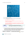
It is essential that the grid is connected as otherwise “artificial slots” appear that will
have a negative impact on the solution as surface current cannot flow over such
locations. Fig 1.6 shows an example of a faulty grid. In practice such places are
hard to detect by inspection of the structure in the Display area. Also in this case
the mentioned tool might offer a significant service.
Fig 1.6: The center nodes of both grids are not in contact with each other.
.This is a grid error as the current cannot pass such a line. Of course this is
unsuitable method for modeling small existing slots! In such a case the
patches close to the slot should not get larger then the slot width.
Once the solution of the problem has been computed, the question arises whether
the results are convergent, numerically stable and reliable. Do the results confirm to
the physical requirements? Checking the credibility of numerical results is not only
strongly recommended, it is a must.
The most important techniques:
•
The inspection of the power budget (input power = radiated power + losses)
•
Physical credibility of results (is the solution at least basically sound)
•
Model variation and parameter variation
•
Check of the boundary conditions
•
Convergence of computed quantities (change in patch size and
segmentation within reasonable limits)
•
Comparison with analytical solutions
•
Comparison with measured data
•
Comparison with the results other numerical methods
1.7 Three essential steps for solving a problem
The following steps are necessary to perform a numerical analysis:
CONCEPT-II, User's Manual
1.7 Three essential steps for solving a problem
13
1. Pre-processing
Important and perhaps time-consuming in practical cases is the discretization
of structures. The programs of the CONCEPT-II CAD tool box can be used,
click on the Cad tools tab (see Fig 1.8, sub window Project view) After the
surface patch structure has been discretized a number of additional input
data has to be entered, such as wire coordinates, loads, kind of excitation,
kind of symmetry, monitor probes, frequency steps etc., click the Simulation
tab and fill the entries of the simulation Project tree.
2. Numerical computation
This step involves setting up the equation system and solving it. Mainly
depending on the number of unknowns N the computation can take a
while. Setting up the system matrix is proportional to N2 and solving the
matrix equation by LU decomposition (standard solver) is proportional to
3
N . This means 8 times in solution time when doubling the number of
unknowns.
3. Post processing
Electromagnetic (EM) fields can be computed at arbitrary positions in space.
Surface current distributions can be visualized, 2D or 3D radiation diagrams
can be computed etc. (tab Post processing)
1.8 Some file names
The CONCEPT-II software package creates a number of ASCII and binary files in
the current working directory. This following list gives a survey on the most
important ones. It is advantageous for the user to know them.
concept.out
Created by the back-end. Contains results if the Print option (Simulation tab,
simulation Project tree) is active. This file contains all current amplitudes, wire
identifiers, number of unknowns, calculated system responses etc. concept.out is
an ASCII file.
conerr.out
Contains error messages and warnings. Please carefully study in case of
unexplainable program failure!
.in files
Almost all executables of the CONCEPT-II package require input data files.
Examples: eh2d.in, plate.in. When existing, these files are automatically loaded by
the GUI.
CONCEPT-II, User's Manual
14
1.8 Some file names
.out files
Many executables of the CONCEPT-II package produce result files in ASCII format.
Examples: concept.out, freqloop.out, eh1d.out
surf.0 → The overall combined surface patch data file of the structure under
investigation. If magnetic symmetry planes are existing only the surface parts that
are in the symmetry plane need to be discretized. surf.0 contains the completed
structure.
wire.0 → Contains the overall and combined wire structure, see remarks for surf.0 .
Tip
It is not allowed to use the file names surf.0 and wire.0
when specifying a structure under the simulation Project
tree
confreq.in → Contains the frequency steps
eh2d.movie → 2D EM field distribution, surface patch data format, data file
co_fmovie.asc
co_cmovie.asc → current vectors to be displayed on surf.0
rad.n → Data of 3D radiation diagrams (surface patch data format)
co_ifl.asc → computed surface current distribution (to be displayed on surf.0)
co_ili.asc → computed wire current distribution
Erasing these two files in a project directory means that the whole perhaps timeconsuming simulation has to be started again.
red-y-mat.asc → Reduced Y matrix/matrices in the case of multi port excitation.
freqi.asc, frequ.asc, freqzin.asc, freqe.asc, freqh.asc → Frequency domain system
responses as a function of frequency, I(f), U(F), Zin(f), E(f), H(f)
contour.asc → contour lines
1.9 Performing a typical simulation
A quick start.
Important for Windows users: Use only file names etc. without blanks!
Some useful and important key and mouse actions: Help → Navigation
It is recommended to start learning the handling of CONCEPT-II by means of the
examples in the $CONCEPT/demo directory. We have 4 examples here and each
CONCEPT-II, User's Manual
1.9 Performing a typical simulation
15
example is described step-by-step. The corresponding PDF files can be
downloaded in addition to this manual and the installation instructions. A detailed
description is also provided for the 'Table-antenna' example
(CONCEPT/examples/Table-antenna), please refer to to Section 2.
A right-handed x,y,z coordinate system is assumed. In case of an ideal ground all
structure parts have to be located in the upper space z> 0. The plane z=0 marks
the ideal ground plane; surfaces and wires may be galvanically connected to it.
1. Start the CONCEPT-II graphical user interface
This can be done by clicking the CONCEPT-II icon or by typing
a) Linux: concept.sh <Enter> in the command line of a terminal
b) Windows: concept.exe (Concept-II-12.0.bat in case of problems)
2. For a new simulation: click File → New simulation
A dialogue opens with input fields for the Project name
and the Project directory. Click Browse to choose an existing directory or to
create a new directory.
In case of a new structure open the CAD tools section by clicking the CAD
tools tab (sub-window Project View, see Fig 1.8)
Discretize the structure to be investigated (wires and/or surfaces), use the
tools under tab Cad tools 2 for this purpose. Simple bodies, cylinders, plates
etc. can easily be discretized by clicking on one of these icons that appear in
the Tool bar:
.
A structure which has already been loaded under Simulation and which shall
be modified can easily be transferred into the CAD tools section: Press the
CAD tools tab, right-click on the top tree entry: Geometry from simulation
→ click on load simulation file(s).
3. For an existing simulation: Click File → Open simulation to open the
simulation. It is a good idea to start with the table antenna example which is
in the $CONCEPT/examples directory.
Input control files for CONCEPT-II end with the suffix .sim.
CONCEPT-II, User's Manual
1.9 Performing a typical simulation
16
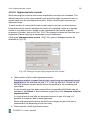
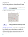
Fig 1.7: Example of the head section of the CONCEPT-II simulation
project tree in 'Project View' section. Here we have the project
Table_antenna from the input control file Table_antenna.sim
Important for users who are familiar with older versions of CONCEPT-II: you
can select concept.in which was the former name of the input file. The
contents of this file will be converted into the new file format which is
completely different, but has ASCII format again.
The Simulation tab is now active.
(Newly created structures of the Cad tools section can be loaded into the
Simulation by right clicking the root tree entry of the Project tree→ select
load all files from 'CAD', see figure below.)
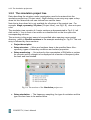
4. Carefully check all items of the project tree. Right click opens a context
CONCEPT-II, User's Manual
17
1.9 Performing a typical simulation
menu which is available in many cases.
Tip
Important for handling of the simulation project tree (section
'Project view')
●
●
●
Right click an item of the project tree. This opens a list
box enabling the selection of dialog windows for
example.
Double-click on an item (for example Surfaces) quits the
sub-tree view.
Another double-click causes the sub-tree to become
visible again
Display area: Surfaces, nodes, wires, edges etc. are always
selected by right click! Rotate mouse wheel: a possiblity to
zoom in or out. Left click and drag: rotate the structure.
Please notice Help → Navigation
Naming of wire files:
name_of_wire_file.wire or wire.name_of_wire_file
Naming of surface files:
name_of_surface_file.surf or surf.name_of_surf_file
Examples:
surf.1, box.surf, surf.box
wire.1, grid.wire, wire.grid
Arbitrary names are possible in principle, however only file names according
to the mentioned rules will be automatically recognized and listed.
5. Choose the number of CPUs (see spin box at the beginning of the tool bar,
see Fig 1.8 ).
6. Start the simulation by clicking on the green Run icon
on the left side of
the tool bar, notice Section 1.5.
The number of unknowns can be taken from the following action before
starting the simulation: Simulation (Menu bar) → Run simulation front-end
→ The number of unknowns appears in the project status view section under
the display area. A new simulation data file is written or an existing file will be
overwritten; default name: concept.sim.
See also tab Log data →CONCEPT-II monitor
CONCEPT-II, User's Manual
1.9 Performing a typical simulation
18
7. After the simulation has finished start the post processing by clicking the
Post processing tab. Output data of the back end run (contents of the ASCII
file concept.out): tab Log data → CONCEPT-II Simulation
Here a number of dialogs are available:
The current distribution on wires and patches can be displayed.
●
Simple rule for a first validation: In general the vectors of the surface
current distribution should follow smooth curves, they should look
“beautiful”. Jumps in current vectors from patch to patch are bad and
cannot be accepted in large areas. The reason for “hot spots” or randomly
distributed current vectors has to be investigated carefully. In many cases
such phenomena are a hint for an insufficient grid (maybe too rough for a
certain wavelength) or a non-convergent result in case of the MLFMA for
example.
16 phase intervals are a good choice for creating movies. Press Animate
to start the movie.
------------------------------------------------------------------------------Right click into the Scale widget → a drop down list opens, select
Arrows,circles... for scaling purposes (alter length of arrows, change
colors, 3D arrows etc.)
-------------------------------------------------------------------------------
●
2D Electromagnetic field distributions can be computed
●
Radiation diagrams can be computed
●
...
Note
Validation of the numerically gained results is a must-do!
8. Hint for users which are familiar with the CONCEPT-II versions prior to
version 12.0:
The whole package can still be operated at the prompt (terminal). This is
recommended in case of an unexplainable behavior. Carefully study the
output appearing on the screen.
Start of the front end:
concept.fe filename.sim <Enter>
CONCEPT-II, User's Manual
19
1.9 Performing a typical simulation
Start of the back end:
concept.be <Enter> → Only a single CPU will be used
Linux:
mpirun -np no_of_processors concept.be <Enter> → The parallel back end
runs with np processors.
Windows:
mpiexec -np no_of_processors concept.be.exe <Enter> → The parallel back
end runs with np processors.
Menu bar
Tool bar
Project tree
Display area
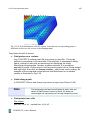
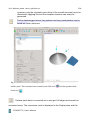
Fig 1.8: The CONCEPT-II main window
The CONCEPT-II main window is shown in Fig 1.8. In contrast to previous versions
it has been designed for full screen usage.
1.9.1 Overview
●
On the left side we have the 'Project View' section. The contents of this part
CONCEPT-II, User's Manual
20
1.9.1 Overview
of the GUI changes depending on the active tab of the 'Project View'
section . In Fig 1.8 the Simulation tab is being active, representing the
simulation project tree. All input data for the numerical simulation (setting-up
and solving the matrix equation(s)) has to be specified here.
●
Display area
◦
◦
Left click, hold and drag causes the structure to rotate
Press keys <Ctrl>+<Shift>, left click, hold and drag → the selected subregion will be enlarged.
Alternative: activate
, left click and drag the mouse pointer. If several
steps of enlargement have been applied get back to the last step by
clicking on
. Show the initial representation by clicking on
.
◦
Press <Ctrl>,left click and drag → the structure is shifted in the Display
area (the same action by clicking on
◦
◦
●
, left click and drag)
Rotate the mouse wheel → structure is zooming in or out, depending on
the direction of rotation; the zooming-in center is the current position of
the mouse pointer.
All shortcuts: Help → Navigation
In the top part we have the menu bar and the tool bar.
The contents of the tool bar changes depending on tab being active in the
'Project View' section.
●
●
At the bottom of the main window we have the project status view section
where information of the currently running simulation is written into
Directly underneath the display area we have a small section (a single line for
text) where patch numbers, coordinates, physical quantities etc. are
displayed on mouse over.
1.9.1.1 Icons of the tool bar
: If the Simulation tab is active the back end starts, setting up the equation
system and solving it. When working under CAD tools pressing this icon may
start a grid refinement or the generation of a surface or a similar action (the same
action is initiated by typing on the <e> key).
CONCEPT-II, User's Manual
21
1.9.1.1 Icons of the tool bar
: The dialogue window for curve representation opens; an example application
is described in Sec. 2.1.2.3. Graphical output is possible in the formats png, svg
and eps (CONCEPT-II gnuplot front end).
Indicates the x-y plane, sometimes helpful when added to the displayed
structure.
: Tool for measuring distances. Select two different nodes by right clicks!
: Loaded surfaces parts appear in different colors
: Switch the grid on/off. Especially useful in case of fine large grids.
: Show normal vectors of all patches
: The end of wires are marked. Modify markers by Cad options → Dot size
(marker, wire ends)...
: Show the segmentation of wires
: (“Picker” icon) By default information on patch numbers, node numbers,
coordinates etc. is shown a small section underneath the display area on mouse
over. In case of very large grids this might lead to an annoying delay when
attempting to rotate the structure in the Display area. Disabling provides a smooth
rotation again, of course depending on the performance the graphics card. It might
be useful to deactivate this feature temporarily on a notebook or a computer with a
less powerful graphics card.
: Enables the rotation of the structure around a selectable point . Right-click a
node and drag the mouse. Known bug: after deactivating this feature the structure
might appear somewhat deformed. Click on
to get the original representation
again.
: The end of wires is indicated by arrows. The reference direction is from the
beginning to the end.
CONCEPT-II, User's Manual
1.9.2 The simulation project tree
22
1.9.2 The simulation project tree
Data describing the structure under investigation need to be entered into the
simulation project tree ('Project view'). Right clicking on an entry may open a dropdown list box where the user can choose from various items.
Note that a drop-down list is not available for all entries of the project tree. For
example Magn, symmetry, XZ plane ('Project View'), see Fig 1.8), does not open
a list.
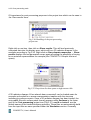
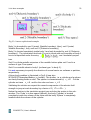
The simulation tree consists of 4 major sections as demonstrated in Fig 1.9. Left
click on the '+' box in front of an entries or a double click on the line opens the
corresponding sub-tree.
The root entry is the project name to be specified when opening a new project
directory, which is Parallel-resistors in the example according to Fig 1.9. The root
entry is followed by these sections:
●
●
●
Project description
Setup structure →Wires and surfaces have to be specified here. Also:
symmetry, types of boundary conditions and surface properties.
Setup monitoring → Set probes for the computation of EM fields or probes
for currents and/or voltages to be displayed as a function of frequency after
the back end has finished.
Fig 1.9: The sections of the Simulation project tree
●
Setup simulation → The frequency sampling, the type of excitation and the
type of solver have to be entered here.
CONCEPT-II, User's Manual
1.9.2.1 Handling of the simulation project tree
23
1.9.2.1 Handling of the simulation project tree
As has been said already: Right-clicking on an entry of the project tree opens a
drop-down list in most cases. Continue by selecting the required menu item.
Example:
A right click on Surfaces provides a drop-down list containing the entries
- Load surface files
- Load all surface(s) from CAD
→
All surface and wire files are loaded from the Cad tools section into
the Simulation section
- Unload all surface files
- A pure metallic structures
→
All dielectric interfaces are turned into metallic surfaces
- Surface impedance
→
A conductivity and a thickness can be assigned a conductivity and a
thickness can be assigned to metallic surfaces
- Thin sheet approximation
→
An electrically thin and geometrically thin lossy sheet can be placed at
one side of a PEC surface
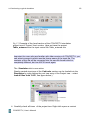
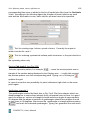
Load all surface(s) from CAD → The corresponding file names appear as
additional entries under Surfaces; an example can be seen in Fig 1.10 where a
surface patch file named surf.1 has been loaded.
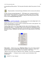
Fig 1.10: Drop-down list for modifying the properties
of a surface patch file, here surf.1
Clicking on Show labels provides the possibility to display node numbers or patch
numbers. It is recommended not to select all numbers for presentation in the case
of large structures. If the numbers are too close to a surface patch file they can be
CONCEPT-II, User's Manual
24
1.9.2.1 Handling of the simulation project tree
shifted into the direction of the patch normal vectors. An example of a simple metal
structure can be found under $CONCEPT/examples/Table_antenna, see Sec. 2 for
a detailed description. The show labels feature can be very helpful searching a
patch by specifying its number only.
1.9.2.2 Dielectric bodies
●
●
Bodies are finite regions in space with homogeneous material parameters,
namely permittivity ϵr and conductivity σ. The user could imagine a lossy
dielectric sphere as a simple example of a body, for details concerning theory
refer to Section 4.
On the surface of a pure dielectric body the following boundary conditions are
matched:
E t , internal =E t ,external
H t , internal =H t ,external
(1)
Parts of a dielectric body may be covered by a metallic surface. In this case
the boundary condition E tan =0 is separately matched on both sides of this
surface. Therefore surfaces that are bounding a body lead to double the
number of unknowns compared to simple metallic surfaces in free space.
Bodies are completely enclosed by two different electric current distributions
in CONCPT-II. One current distribution is “responsible” for the internal EM
field and the other one makes the external EM field. Both can be visualized.
●
Surfaces that are bounding a dielectric region (a body) have to be completely
closed.
Surfaces are not possible in a symmetry plane; the user can think of the
structure being completed on the other side of the symmetry plane, again
yielding a completely closed overall surface.
●
●
●
Wire can be placed in bodies. If a wire is penetrating a surface of a body, this
wire has to be split into two parts: both sections must be attached to the
same surface patch node, i.e. the wires sections must end at the same patch
node. All patches sharing this node will be metalized automatically.
Structure parts (wires or surfaces) inside dielectric bodies have to be
discretized according to the internal wavelength.
Metal cavities with a small aperture in air and filled with air can be considered
as bodies: the apertures are modeled by a surface were the boundary
condition (1) is matched. On the cavity wall which is described by another
boundary Etan=0 is matched separately at the internal and external side.
Such a proceeding may be advantageous for a careful analysis of coupled-in
EM fields. Note: Defining a completely closed metallic cavity as a body
makes no sense.
CONCEPT-II, User's Manual
1.9.2.2 Dielectric bodies
●
●
●
25
Surfaces where the boundary condition (1) is specified can be layered by thin
lossy dielectric or lossy magnetic sheets. The thickness of such sheets
should not be larger then 5...6 times the penetration depths resulting from the
layer material.
The typical dimension of bodies that can be computed depends on the
internal conductivity – if it is too high the solution may become unstable.
Rule: All patches of a (sub)surface bounding a body should have the same
two regions on both sides.
More details concerning the modeling of bodies are given in Secs. 3.1 and 4.
Examples:
$CONCEPT/examples/Three_cubes,
$CONCEPT/examples/Parallel_resistors,
$CONCEPT/examples/Bodies_in_bodies
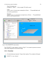
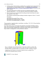
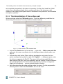
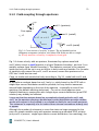
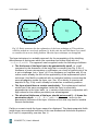
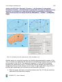
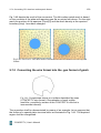
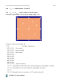
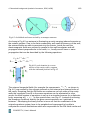
The procedure to specify bodies is as follows, see Figs. 1.12 1.13 1.15 and shall be
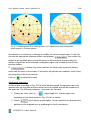
explained by an example.
As can be seen in Fig 1.11 we have two quarters of a cylinder attached to each
other. Due to symmetry the problem comprises a full cylinder on an ideal ground
plane with two bodies separated by an internal surface. Each cylindrical section
may include a homogeneous (lossy) dielectric material.
Fig 1.11: Example of two bodies attaches to each other on ideal (x-y plane). The
assumed magnetic symmetry plane is the x-z plane. We have 5 surfaces bounding
the bodies. The top and blue surface are assumed to be PEC. Assuming a certain
conductivity in the bodies we can model a parallel resistor (example from
$CONCEPT/examples/Parallel_resistors)
CONCEPT-II, User's Manual
1.9.2.2 Dielectric bodies
26
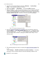
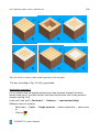
1. Load the surfaces describing the structure: Surfaces → Load surface
file(s). In our example we have 5 surfaces
2. Right click Bodies → Add bodies → a new entry body 1 appears
3. Right click body 1 → the drop-down list shown in Fig 1.13 appears. Now the
surfaces covering body 1 can be selected either by mouse over (right-click
on the corresponding surface) or by editing a list that appears when choosing
Surface selection by edit. Continue in the same way defining body 2
Fig 1.12: Surfaces forming two bodies
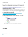
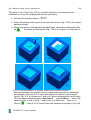
4. Next the material parameters for the bodies have to be entered. Select for
example body 1 → select Set material values Fig 1.13 → A dialogue opens
where the parameters ϵr and σ can be entered. Double clicking on the
input field Body name enables to change the default name “body 1” to an
arbitrary name.
Fig 1.13: Defining the bodies from the surfaces
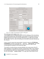
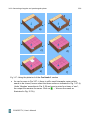
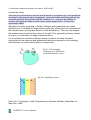
5. The remaining step to be done is to specify the type of the each surface (Fig
1.12):
Select Surfaces → Metallic and dielectric surfaces (bodies) → A window
as shown in Fig 1.14 opens where to enter the boundary condition to be
CONCEPT-II, User's Manual
27
1.9.2.2 Dielectric bodies
applied to all surfaces.
●
Metallic boundary
Always the PEC part of a body boundary. Caries two current distributions:
one contributes to the the internal fields of a body and the other one
contributes to the external field of the body.
●
Dielectric boundary
Both tangential components of the EM fields are matched here; again with
have two current distributions.
●
Free space
If there is a surface in spree space, i.e. outside the specified bodies it
would be given this property, meaning metal in free space (EFIE problem
with a single layer current distribution). Such a surface is not allowed to
bound a body.
●
In body 1, In body 2,...
The user could think of a ideal conducting metal disk for example
completely immersed into the material of body 1 or body 2, respectively.
Again, such a surface is not allowed to bound a body.
In Fig 1.14 the blue and red top surfaces are assumed to be ideal conducting
metal plates of type Metallic boundary and all other ones are of type Dielectric
boundary.
Surfaces can be layered by geometrically thin sheets, see Fig 1.15. Selecting Add
layer enables to enter the material properties.
Fig 1.14: In the example case the top
plates are of metal whereas all other
surfaces are dielectric interfaces.
Note
Layers are only possible on surfaces of bodies.
Layered surfaces must be of type Dielectric
boundary. For details see Secs. 3.1, 3.1.6,4
CONCEPT-II, User's Manual
1.9.2.2 Dielectric bodies
28
Based on the given information the user is invited to carefully study the examples
under $CONCEPT/examples/parallel-resistors and $CONCEPT/examples/Threecubes.
In case of a body that is positioned completely inside another body with no common
boundary (the user could think of two sphere with the same center but different
radii) further information needs to be entered:
(right click) Body in body → Assign → a window opens where to enter which body
is inside another body. In the example $CONCEPT/examples/Bodies_in_bodies a
structure is treated where we have a spherical body inside a cylindrical body which
again is completely inside a cube. In addition we have an open PEC cone inside
the cube, not in touch with the other bodies.
The user must be very careful specifying the “body in body” information:
CONCEPT-II does not check if the data is correct.
By default all bodies are immersed in free space, which is body 0. The topic is
further explained under Section 3.1.4.
Fig 1.15: Adding a layer to surf.4. Clicking on Add layer open a dialogue
where to enter the material parameters and the thickness
1.9.2.3 Wires
CONCEPT-II, User's Manual
29
1.9.2.3 Wires
Fig 1.16: The drop-down list related to wires
Various features exist for wire treatment, see Fig 1.16. Similar to surfaces, wires
may be organized or grouped in different files which should begin with “wire.” or
end with the suffix “.wire”; wire.1 or concept.wire are examples for valid names.
Add wire files(s) → existing ASCII files in the CONCEPT-II specific data format
(see Sec.3.10) can be loaded into the simulation.
Selection of Edit a new wire file opens a dialogue window where all required data
such as the file name, number of wires, coordinates, radii and number of basis
functions (number of wire segments) can be entered.
Note
Deactivation of the check marks in the small boxes in front
of the loaded wire files or surface files let the corresponding
structure parts disappear in the display area. This does not
mean that they are deleted from the simulation!
It is important that the thin-wire assumptions are not hurt, notice the corresponding
remarks under Sec. 1.6.1. Basic errors in wire modeling are detected once the
check box Check wires is active. Wires with errors are marked red, warnings
appear in pink.
For each wire the number of segments (basis functions) has to be entered.
● It is recommended that 3 segments are specified on electrically short
sections which appear under the following circumstances:
◦ Wire-grid modeling where surfaces are simulated by corresponding wire
grids; each wire being electrically short in general.
◦ Short wires which connect different surfaces. Such wires are important
from a network point of view to model an existing galvanic connection.
◦ Short pieces of vertical wires, connecting lines to ground.
●
●
Rules for discretization have already been given Sec. 1.6.1.
If it turns out that the initial discretization of a wire is not sufficient when
increasing the frequency in a frequency loop the number of basis functions
CONCEPT-II, User's Manual
1.9.2.3 Wires
30
will be automatically increased according to the specified number of basis
functions per wavelength.
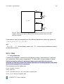
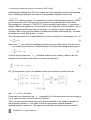
Fig 1.17: Wires attached to a surface patch node common to four triangles.
Left: the ratio of radius over edge length of the triangles is ok.
Right: the radius of the wire is far too large compared to the edge length of the surface
patches. This is already a problem which would require a 3D surface patch grid. Note that
in case of a wire a simple line current is flowing along the axis, testing the boundary
condition is not accomplished around the circumference.
Wires can be connected to the surfaces patch nodes of metallic surfaces and to
other wires. Connections are recognized if the difference in coordinates is smaller
than 10-5 of the applied unit (default is meter) . A triangular patch is allowed to have
one or more wires attached to a single edge, hence there must be always 2 edges
between different points of attachment in a triangular grid. Wire identification
numbers are written into concept.out . By these numbers can be assessed if a
galvanic connection has been recognized or not.
As explained by means of Fig 1.18 it is not allowed that wires intersect with each
other somewhere along their extension. In case of a physical point of attachment
straight wire section must start or end at that point.
CONCEPT-II, User's Manual
31
1.9.2.3 Wires
W1
a)
W1
W2
Wrong!
W2
b)
W3
Fig 1.18: In a wire junction wires must start or end
a) Wire 1 intersects with wire 2, a junction is not recognized. An error
message is given
b) If wire 1 shall be calvanically attached, three wires are necessary meeting
in the common point of attachment
Both surfaces and wires can be loaded by lumped elements R, L, C in various
combinations.
Select a wire file in the simulation project tree → (right click) → Set loads →
dialogue window opens for the specification of loads (possible positions: beginning,
middle and end of a wire), various predefined circuit elements are available. An
example is demonstrated in Fig. 1.19: we have a series connection of a resistor and
an inductor ,R,L positioned in the center of wire 1, 2, ….
In case of a large number of loads:
•
•
•
•
•
Append the corresponding number of lines (“Total loads”), click OK
Right clicking into the 'Wire no.' field provides the possibility to set all wire
numbers at once.
The same holds for all other positions. Right clicking on 'Circuit identifier'
gives Set global. Activating gives a selection of various circuit identifier. The
chosen identifier can be assigned to all wires.
Loads can be taken from files. Format: frequency real part imaginary
part (three real numbers in each line)
For inserting, deleting or copying of a line ('Load 1', 'Load 2',... , see Fig 1.19)
right click on 'Load 1' or 'Load 2' or whatever load number shall be selected
CONCEPT-II, User's Manual
1.9.2.3 Wires
32
Fig 1.19: Dialogue window for specifying lumped loads
For placing lumped loads on surfaces (at least one surface files must be loaded):
right-click the project tree entry → Load(s) on patch edges → Set edge loads →
a dialogue window opens.
Select an edge between two patches by a right click. A load symbol is located at the
chosen edge, specify the circuitry identifier and the R, L, C values.
For voltage probes: select Voltage probes on patch edges by a right click → Set
Probes→ select the probe at the required position.
1.9.2.4 Frequency sampling
In Fig 1.20 all main entries of the Setup simulation section of the project tree are
illustrated (Frequencies, Excitation, Solver) . Right-click on Frequencies gives
the shown drop-down list.
Fig 1.20: The Setup simulation section of the simulation project tree
Note that a special frequency sampling is required if an inverse Fourier transform
shall be applied for time-domain system responses.
CONCEPT-II, User's Manual
1.9.2.4 Frequency sampling
33
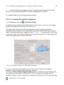
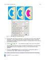
Fig 1.21: Window for setting the frequency sampling
Clicking on Frequency loop for a special interval → right click Set values opens
a window for specific entries, see Fig 1.21. Clicking on Generate value list gives
the list in the 'Used frequencies' area. It is possible to add values “by hand” here or
to edit an existing list of frequencies. In the example the interval between 1 MHz
and 5 MHz is sampled by 0.7 MHz steps. Note that the last step comprises only 0.5
MHz. Click on OK to activate the selection.
The next logical step when setting up a simulation is to specify the type of
excitation. According to Fig 1.22 a number of responsibilities are existing.
CONCEPT-II offers the possibility to compute time-domain system responses
based on an inverse Fourier transform IFT. A careful selection of the frequency
interval and of the frequency sampling is required; details can be found in Sec.
3.8 .
Fig 1.22: Excitation variants
How to use Stochastic EM excitation is not yet described in this manual. The
CONCEPT-II, User's Manual
1.9.2.4 Frequency sampling
34
results of an application have already been published:
M. Magdowski, A. Schröder, H.-D. Brüns, R Vick: Effiziente Simulation der
Einkopplung statistischer Felder in Leitungsstrukturen mit der MoM, EMV
Düsseldorf, 2014, Seiten 238-244.
Simulation of coupled-in quantities in a mode stirred chamber.
1.9.2.5 Voltage generators
Voltage generators can be located both on wires and surfaces (edge generators).
To specify one or more voltage generators the following steps are necessary:
Generators on wires
Excitation → Voltage generator(s) → Generator(s) on wire_file_name (example
antenna.wire) → Set generator(s) → a window according Fig 1.23 opens.
Position the mouse pointer on the wire where a generator shall be located. Right
click selects the wire and a new line appears in the input window. Next set the
position of the generator. Three locations are possible: 1st segment, middle
segment, last segment.
Of course we can also enter a voltage generator by appending a line (click the OK
button, Fig 1.23) and entering the wire number by hand. The wire number is shown
directly under the display area when placing the mouse pointer accordingly.
Fig 1.23: Window for the specification of voltage generators on wires
Delete a generator: Click on entry 'Generator no.' at the beginning of the
corresponding line →the line is marked. Right click on Generator no. → Delete
Voltage generator on an edge between adjacent patches (edge generator)
CONCEPT-II, User's Manual
1.9.2.5 Voltage generators
35
Select item Generator(s) on patch edges in the project tree → right click → Set
edge generator(s) → click on the required edge of the surface in the display area.
For a change of polarity right-click on the same edge again. Specify voltage
magnitude and phase in the window that has been opened.
1.9.2.6 Ports
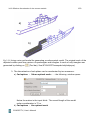
In practice it is frequently of interest to compute only the mutual coupling of a
system at feed points (voltage or power generators), located at different positions of
the structure under investigation – one could imagine a ship carrying a number of
monopole antennas. Such feed points are designated as ports. As demonstrated in
Sect. 3.2 the mutual interaction between ports can be described by a reduced
admittance matrix of order K, where K is the number of ports, which have been
defined. In general K is much smaller than the order N of the system matrix.
Right mouse click on the item Excitation in the project tree → Ports (power input/
voltage input)
If both wires and surfaces are in the simulation the following project tree entries
appear (wire_file_no: name of the wire file):
Port(s) on wire_file_1
Port(s) on wire_file_2
…
----- Ports on patch edges
Right-Clicking on Port(s) on wire_file_1 → Set values opens a dialogue window as
depicted in Fig 1.24.
CONCEPT-II, User's Manual
36
1.9.2.6 Ports
Fig 1.24: Example of three ports, each defines a power generator in the center
of a wires 1,2,3 of the the wire file concept.wire
Note
Note that generators (power or voltage generators) do not
excite the structure 'at the same time' in case of ports. The
tools under Post processing provide the possibility to
select which port is the active one. All other ports are short
circuited. Loads which may be defined at the position of
ports are not effected.
Note: appropriate wires can selected by right-clicking on them in the display area.
Then choose the required location (middle, last, 1st segment) then.
In case of an edge generators choose Port(s) on patch edges → Set edge port(s)
→ a dialogue window opens. Select the required edge for a voltage or power
generator by a right mouse click. Change generator polarity by a second click on
the same edge.
Defining ports enables the computation of S-parameters between the ports. In
addition to this a file named red-y-mat.asc (various formats available) is generated
containing the complex admittance matrix for each frequency step. Each matrix is
describing the coupling between the ports. In the example case according to Fig
1.24 we have three ports, hence the admittance matrix will be of order 3x3.
CONCEPT-II, User's Manual
1.9.2.6 Ports
37
For further details refer to Sect. 3.2 .
●
●
The sequence of the generators including the corresponding edge
coordinates and reference directions are written into the file patchgen.in
(default name).
It is important that adjacent generator symbols of a common feed region are
pointing into the same direction (example: generators around a cylindrical
section)!
1.9.2.7 Plane wave field
Setting all angles to zero provides a plane wave propagation against the z axis with
the E vector directed in the positive direction of the x axis. The E vector can be
rotated around the k vector by the polarization angle Ψ.
Fig 1.25: Input fields for defining a plane wave excitation.
CONCEPT-II, User's Manual
1.9.2.7 Plane wave field
38
Fig 1.26: Data input for elliptic polarization
For elliptic polarization we have the following initial position:
The vector with with amplitude E1 is pointing in positive x direction and the vector
with amplitude E2 is pointing in the negative y direction. Both vectors are
perpendicular to each other. The phase angle, which refers to E2 determines the
direction of rotation for elliptical or circular polarization.
Fig 1.27: Orientation of the E field vector and the wave
vector based on the values as given in
Rule: The sense of rotation is determined by rotating the phase-leading component
towards the phase lagging component. The field rotation is observed as the wave is
viewed as it travels away from the observer (looking into the direction of the wave
vector k). The values according to Fig 1.26 lead to a situation according to Fig
1.13, that is we have a right circularly polarized wave (RHC: right hand circular
polarization, clockwise rotation). Rotating the k vector into the positive z direction
and the E1 vector into the positive x direction we have:
E x= E1
sin (ω t−β z ) , E y =E 2 sin (ω t−β z+δ) with δ as the Phase angle.
Assuming a positive phase angle the sense of rotation is left hand (LHC) .
CONCEPT-II, User's Manual
1.9.2.8 Impressed wire current
39
1.9.2.8 Impressed wire current
Wires carrying line currents with known amplitudes can serve as excitation. The
induced currents on the other surfaces and wires that might be present have no
impact back onto the exciting wire currents. Hence these known currents are
impressed ones.
A short section of a wire with known current may be used as a current source.
Long wires can be used to simulate the stroke of a lightning, either as a nearby
stroke or as a direct stroke, based on the transmission line model originally
proposed in [Uman], see end of Sec. 3.8.4.The channel is taken into account by a
sequence of wires carrying an impressed current distribution.
Clicking on Impressed wire current (Fig 1.22) opens a dialogue window as
depicted in Fig 1.28.
Fig 1.28: Dialogue for specifying impressed wire current
●
Total number of wires with impressed current
Entering a number n means that the last n wires carry an impressed current
distribution. In the example we see a “1” in the top spin box. Hence the last
wire has a known current distribution to be specified in the remaining two
input fields.
If only a single wire has been entered the corresponding EM fields can be
computed, see Solver in the simulation project tree, item Compute only the
impressed field.
If a short piece of wire with an impressed current is part of a loop it is
possible to model an ideal current generator.
Wires with impressed currents should form a sequence (end of a wire is
connected to the beginning of the next one).
●
Phase velocity of the impressed current
CONCEPT-II, User's Manual
1.9.2.8 Impressed wire current
40
In case of a lightning simulation the relative propagating speed of the timedomain current function.
0 → All basis functions have a constant amplitude all over the wire(s) with an
impressed current distribution. Useful to model a current generator.
1 → Propagation with speed of light (0.333 is frequently taken for lightning
simulations).
●
Amplitude of impressed current in kA
For more information refer to Sec. 3.8.4
1.9.2.9 Solvers
The last section of the simulation project tree concerns the selection of the solver,
Fig 1.29. The number of processors to be used can be entered in the upper left
Fig 1.29: Solvers in the CONCEP-II package
corner of the main window, right to the green light button.
Details with respect to memory and computation time have already been mentioned
in Sec. 1.5 and Sec. 1.7.
For LU decomposition with row pivoting it is advantageous to select the number of
CPUs according to a quadratic number: 4, 9, 16, 25,....This rule does not apply to
MLFMA.. Never enter a number larger then the number of CPUs available on the
computer!
Note
Application of the ACA or the MLFMA solver: the typical
dimension of the structure under consideration has to be
electrically large. Triangular meshes are preferred!
CONCEPT-II, User's Manual
1.9.2.9 Solvers
41
ACA is currently only available for single CPU usage and pure surface patch
structures in free space. LU decomposition is the default solver which can be
applied to any kind of structure.
A major limitation of the MoM for electrically large objects is the very large
Fig 1.30: Default entries for the MLFMA solver
computation time and the huge amount of RAM space that is necessary. The
MLFMA reduces both storage and CPU time requirements significantly to N log (N).
In case of the ACA we have an N 4 /3 log N proportionality. The MLFMA solver can
only be applied to metallic structures including wires and surfaces and symmetry.
Residual tolerance: Determines the precision of the iterative numerical solution.
0.01 could be sufficient in case of far field computations. 0.0001 could be
necessary for almost closed cavities and complex structures.
Max. number of iterations: If the Residual tolerance is not achieved after this
number of iterations the computation stops.
Drop tolerance for SPAI: Determines the sparsity of the preconditioner. The smaller
the number the more dense the preconditioner and the faster the convergence.
Disadvantage of a small number is a long set-up time.
In the case of plane wave with no structure being present or in the case of an
impressed current distribution with no further structure parts, the item Compute
only the impressed field can be selected.
1.9.2.10 Precision of the numerical solution
The default matching technique is line matching which is fast and gives good
results for freely radiating antennas/structures. Galerkin matching provides even
more precise results with the disadvantage of requiring a higher matrix set-up time.
Cases where a high degree of precision is required:
CONCEPT-II, User's Manual
1.9.2.10 Precision of the numerical solution
●
Very low frequencies, typical structure size 1m and below
◦
◦
●
No problem in case of pure wire structures, see
$CONCEPT/demo/example1-wire-loop for example.
Problem to compute the proper (very small) real part of the input
impedance in case of loops where both wires and patches are involved.
No problem at higher frequencies. No problem in case of pure patch loops
or monopole antennas modeled by strips of patches (triangles).
Cavities with small apertures, where coupled-in or coupled-out field quantities
are of interest: use Galerkin matching; three integration points are normally
sufficient (Fig 1.31)
➔
➔
●
42
No problem with wire antennas inside or outside the cavity and the
wires being not attached to patch nodes.
Problem in case of wire antennas that are attached to patch nodes.
Workaround here: model monopole antennas by small patch strips and
use edge generators. The following equation gives the width w of the
stripes: w= 4 r with r as the radius of the original wire.
Single precision: Experience has shown that the single precision mode only
gives valid results for well-conditioned problems with external excitations in
conjunction with iterative solvers (e.g. MLFMA). For direct solvers or
problems involving cavities use double-precision instead (default).
Fig 1.31: Galerkin matching can only be used in case
of a pure triangular mesh
CONCEPT-II, User's Manual
1.9.3 Post processing tools
43
1.9.3 Post processing tools
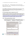
When clicking on the Post processing tab, the 'Project View' section looks as
depicted in Fig 1.32. All programs for post-processing purposes can be found here.
For the application of these programs the CONCEPT-II back end must have been
finished.
Fig 1.32: The post processing project view and project tree, respectively
Under 'Project View' 15 buttons arranged. Clicking on a button opens the
CONCEPT-II, User's Manual
1.9.3 Post processing tools
44
corresponding dialog window. Tool tips give information about the purpose of each
tool.
→ Representation of current/charge distribution both on wires and surfaces.
At least 16 phase intervals between 0,...,360 degrees are recommended for a
movie of the current distribution. If the movie is running to fast enter an integer
value (10,20,... depending on the graphics card) into the Delay spin box at the
bottom of the Post processing section.
Features:
Scale widget: surf.0 is selected → the color map in the scale widget right to the
display area refers to the surface current distribution
Default representation is current vectors combined with colors on the patches. The
colors are indicating the magnitude.
Scaling: Right-click on the Scale widget (section right to the Display area, which
automatically opens) → A number of items can be selected for modification of the
displayed data. Changing the scaling has only an impact on the data belonging to
the actual surface, indicated in the drop-down list in the head section of the Scale
widget.
Color scale → Default color map is Rainbow Colors. The red and blue marked
surface areas can be extended (the color red is shown between a value to be
chosen and the maximum value. Blue colors indicate small values.
Different color maps such as 'Rainbow colors' (default), 'Hot colors' are available.
Arrows, circles... → Scaling of vectors, surface current distribution, field
distributions.
CONCEPT-II, User's Manual
1.9.3 Post processing tools
45
Smooth → Show only a single color per patch in turn-off mode. When hovering the
mouse pointer over a patch the value of the depicted physical quantity is shown
underneath the Display area.
Note
The contents of the vertical value list right to the color bar as
depicted in the Scale widget may change a little, depending
on the mode of representation.
dB values → Current distribution in dB scale
Clicking on Arrows, circles... opens a dialog according to Fig 1.33 .
Fig 1.33: Dialog for the modification of
vector representation
Tip
The mentioned features for vector representation of surface
currents apply also to the vectors of electromagnetic fields.
Scale widget: wire.0 is selected → the color map in the scale widget right to the
display area refers now to the wire current distribution.
Scaling: Right-click on the Scale widget → As has been described for surface
current distributions a number of items can be selected for modification of the
displayed current distribution.
A black arrowhead indicates the current direction at the beginning of the wire. In
case of a change of sign in the current distribution an arrow with a different color
appears at the corresponding location pointing in the reverse direction.
CONCEPT-II, User's Manual
46
1.9.3 Post processing tools
Scaling: Right click into the scale widget → Arrows circles → Lengths, widths, and
colors of the arrows can be changed
For displaying the current distribution on wires as curves click on
in the tool
bar. The following window pops up:
Fig 1.34: Wire current distributions as curves
Right click on the wires whose current distribution are to be shown. ASCII data are
available, see header of the respective files, for example w1-curr-dist.asc, w2-currdist.asc... Clicking on OK provides the curve(s) in a gnuplot preview window. For
more display possibilities right click on the Current wire distr. item in the View
results tree. The CONCEPT-II gnuplot front end opens. Among other features .png
and .svg graphics files can be generated.
→ Dialog window for 3D radiation diagrams opens
Electric far field, EM near field distribution, magnitude, theta components, phi
components
●
The field values are computed on a spherical grid in a
a number of steps to be specified in each direction
●
Δ θ, Δ φ region with
●
Complex far field data for E are stored
●
Movies of 3D radiation diagrams developing as a function frequency
→ Display 2D radiation diagrams
CONCEPT-II, User's Manual
1.9.3 Post processing tools
●
●
●
47
Electric far field in orbit plane of arbitrary direction. The orientation of the
plane can be chosen arbitrarily – the corresponding angles are explained in
the window.
The diagram plane can be displayed together with the radiating structure
Magnitude, theta and phi components, LHC and RHC, gain in the case of
port excitation (power input).
→ Computation of 2D electromagnetic field distributions in rectangular flat
areas.
Subsequent dialog opens for field representation. Movies are possible.
●
E field, H field, Energy flux density, specific absorption rate
→ Computation of electromagnetic fields at an arbitrary position in space.
Observation points can also be set along straight paths in space or can be taken
from a file.
In case of a frequency loop fields are computed for all frequency steps.
→ Computation of EM fields.
If the check box 'Fast parallel field computation' is active a fast computation of field
plots of electrically large areas is possible under the following conditions (status
Oct. 14):
●
No wires and only triangular patches are present
●
Free space, structure not over ideal ground
●
No symmetry planes specified
●
At least 2 CPUs are necessary
'Treatment' ACA → the adaptive cross approximation is used to speed up the
solution. Details about the technique have been published here:
A. Schröder, H.-D. Brüns, C Schuster: Fast Evaluation of Electromagnetic Fields
using a Parallelized Adaptive Cross Approximation. IEEE Transactions on Antennas
and Propagation, vol. 60, no. 12, pp 6058-6061, Dec. 2012
CONCEPT-II, User's Manual
48
1.9.3 Post processing tools
Fig 1.35: E field distribution with 3D vectors. Note that the corresponding phase is
indicated in the lover left corner of the Display area
Drop down list with 3 entries:
●
Field probes on a surface
Any CONCEPT-II surface patch file may serve as input file. The probe
positions correspond to the centroids of the patches. A subsequent dialog
opens, asking for data that are necessary for displaying the result.
Specifying an appropriate 'Number of phase intervals' it is possible to
generate a movie. Further action: set the mouse pointer on the 'Scale widget'
and right click, then click an Arrows, circles... and do the vector scaling. An
example of the computed normal electric field distribution on a metallic
surface is illustrated in Fig 1.35
●
Fields along a path
A CONCEPT-II file in wire format may serve as input (see Section 3.10)
Note
●
The beginning and end coordinates of each wire are
taken as field points! Hence at least 10 wires per
wavelength are necessary in the high frequency case.
Field points from a file
File format:
first line: x1 y1 z1 , second line: x2 y2 z2 , ….
CONCEPT-II, User's Manual
49
1.9.3 Post processing tools
Clicking on Compute starts the field computation. The field points are shown
as small spheres, the color indicating the field strength value. Setting the
mouse pointer on a sphere make the field strength value appear under the
display area.
Provided that that the check box 'Compute field values for all frequencies'
has been activated one may step through all frequencies.
Clicking on the Plot of EM fields icon
(see Tool bar) opens a dialog
where to specify a file name. Set the mouse pointer on a field point and right
click; the selected point becomes white. The data belonging to the selected
point are written into the specified file. The gnuplot front end is used to show
the result.
The described proceeding is also possible for the entries Fields on a
surface and Fields along a path
Clicking on
(see tool bar) enables the user to compute EM fields along
a path.
→ Plot system responses as a function of frequency. A drop-down list shows
the system responses that are available.
Examples: E(f) (Probes from monitoring) → Field point have already
been
set in the simulation phase before the back end has been
started
E(f) (Post processing) → Fields have been computed after the
back end run, tool:
→ Enables the analysis of a transient system excitation, i.e., computing timedomain system responses. Precondition is that a special frequency loop has been
chosen: Simulation → Frequency → Frequency interval for inverse Fourier
transform.
Note
In case of an IFT: Both the limits and the proper sampling
of the covered frequency interval are important for a
successful application. Computation may be timeconsuming as a number of frequency steps are necessary,
depending various parameter such as typical dimansion of
the structure, signal duration and rise-time.
CONCEPT-II, User's Manual
50
1.9.3 Post processing tools
→ Allows the representation of an antenna input impedance in the form of a
Smith chart (program smith). Also representation of port impedances.
→ The current distribution on wires can be displayed. Currently only of
importance for a sequence of time steps in case of an inverse Fourier transforms.
Here the the corresponding wires must have been selected under Simulation (front
end run).
→ Plot of S parameters in case of a port excitation. Definition of ports:
Simulation → Excitation → Ports (power input/ voltage input)
→ Computation of the power flow through a surface (numerical integration of
the Poynting vector over a surface). The simplest way to create such a surface is to
click Cad tools → icon Sphere
. Only triangles are allowed for the integration
surface!
→ Computation of line integrals of E or H, see Section 3.4.
→ The results of an RCS calculation can be displayed (monostatic radar
cross section)
→ EM fields when port excitations are modified
To display the whole structure under investigation click on the Build-geometry icon
. Depending on the kind of magnetic symmetry the icon appears differently. Full
icon color means no symmetry has been specified.
CONCEPT-II, User's Manual
51
1.9.3 Post processing tools
Of importance for post processing purposes is the project tree which can be seen in
the 'View results' area:
Fig 1.36: Handling of the post processing
project tree
Right-click on an item, then click on Show results. This will load previously
computed data into the display area, which will be a 2D radiation diagram in the
example according to Fig 1.36. Right click on Freq.-domain responses → Show
results displays the last generated curves again providing the possibility of tuning
for an external representation for example (the CONCEPT-II Gnuplot front end
opens).
Fig 1.37: Drop-down list that opens on right mouse click
A 3D radiation diagram (if has already been computed) can be loaded again for
example and scaled for a proper representation together with the structure
including its surface currents. Once a 3D radiation diagram has been loaded, the
entry rad.1 (file with surface patch format) appears under Surfaces in the lower
part of the Post processing project tree (Fig 1.37). surf.0 and wire.0 are the
default names of the loaded structure geometry. These files are automatically build
from the input files as were specified under the Simulation section. Generally
CONCEPT-II, User's Manual
1.9.3 Post processing tools
52
surf.0 includes the combined surfaces patch files and wire.0 contains the wires of
all wire files.
Clicking on Move/scale... opens a dialogue by means of which a structure scaling
can be accomplished. Important: this does not change the structure itself; it is only
for graphical purposes. Note further that a 3D radiation diagram is scaled into a
cube of unit edge length, hence its size needs to be altered and/or shifted in most
practical cases, when depicted together with the structure under investigation.
Fig 1.38: Antenna on a table with 3D radiation diagram and 2D field distribution
Fig 1.37 show an example where 3 different results are shown in a single picture.
Noticeable in the drop-down list according to Fig 1.37 is the item Unload data by
means of which the data (surface current distribution for example) can be erased.
Right click on the Surfaces item, see Fig 1.37 offers the possibility to load
additional surfaces to be displayed in the display area. By means of Load data
corresponding field or current distributions can be added (see Section 1.8).
2 Example: Top-loaded wire antenna on a table structure
The handling of the GUI shall be demonstrated by a simple example.
The input files of the following structure can be found under
$CONCEPT/examples/Table_antenna. A top-loaded monopole antenna which is
located in the center of a metallic platform shall be analyzed. The whole structure is
placed on an ideal ground plane. The platform has a height of 0.5 m and consists of
a top plate and two side plates being connected to the ground. The size of the top
plate is 2m x 2m. The length of each wire is 0.75 m. There is an additional wire
CONCEPT-II, User's Manual
The handling of the GUI shall be demonstrated by a simple example.
53
between the top plate and ground modeling a coaxial feeding cable. The electrical
and geometrical symmetries involved in the configuration shall be exploited and the
frequency interval between 1MHz and 100 MHz is of interest.
The structure can be discretized with the CONCEPT-II CAD tools (notice that the
CAD tools tab is active, we have top.surf, side.surf, antenna.wire and coax.wire).
As the vertical antenna is fed, magnetic symmetry can be exploited (x-z plane and
y-z plane). Hence there is only need to specify the geometry in the first quadrant of
the Cartesian coordinate system as illustrated in Fig 2.1. In the example directory
the ASCII file Table_antenna.geo is available for usage in conjunction with the
gmsh tool, see Secs. 3.7 and 1.6. By this file the plates can be discretized outside
the GUI. The corresponding data can be converted into the CONCPT-II surface
patch data format (Menu bar, Import/export).
Fig 2.1: The top loaded antenna with supporting structure
Note
General rule: in the case of magnetic symmetry only the
symmetric part of the structure needs to be discretized.
The ideal ground plane always corresponds to the x-y
plane.
Remember: a magnetic symmetry plane is characterized be E field vectors which
CONCEPT-II, User's Manual
The handling of the GUI shall be demonstrated by a simple example.
54
are completely tangential in the plane of symmetry. On the other hand the H field
vector have only perpendicular vector components there. We observe a dual
situation on an ideal ground plane which is assumed to be present in this simulation
example (x-y plane).
2.1.1 The discretization of the surface part
We are working under the CAD tools section. There are different possibilities for
discretizing the structure. One way shall be sketched shortly.
Fig 2.2: Corner nodes of the antenna table
●
●
●
Activate the Points item in the cad tree → right click → Edit a new point file
and enter all corner coordinates into the dialogue window which opens, see
Fig 2.2.
Activate the radio button Plate, arbitrary quadrangles and select the four
points marking the top plate by right click. Update → a dialogue opens, enter
the data as suggested in Fig 2.3. The name of the surface patch file has
been entered (top.surf), also the frequency and the number of basis functions
per wavelength. Note: for electrically small plates the number of segments
might not be sufficient → correct manually under. Meshes.
Next discretize the side plate and then enter the wires. For this purpose the
following section under the Cad tools 1 tab can be used:
CONCEPT-II, User's Manual
2.1.1 The discretization of the surface part
55
The end coordinates of wire 1 correspond to the starting coordinates of wire 2. So
the code recognizes a galvanic connection between them.
Fig 2.3: Meshing of the top plate. Notice the description of the various input fields
Next click on the Simulation tab (Project view) -> click on head entry concept →
(right click) → Load files fron 'CAD', continue to set up the simulation, moving
through all menu items of the Simulation Project tree, starting at the top.
According to Fig 2.5 all symmetry planes have been activated already (see check
marks under Symmetry). This is also indicated by small yellow cylinders,
appearing in the top left corner of the Display area. Ideal ground (always at z=0.!)
has been activated, which is indicated by the following symbol:
(change of
position: <Shift> + click on the mouse wheel). Select Antenna.wire and right click
→ Edit wires → a dialogue window according to Fig 2.4 opens.
CONCEPT-II, User's Manual
2.1.1 The discretization of the surface part
56
Fig 2.4: Dialogue window for editing wires
Right-clicking on a wire number appearing in front of each row provides the
possibility of quickly inserting or deleting a line (a wire). For rapid global changes in
case of many wires use the drop-down list left to Total wires.
A Number of basis functions per wavelength smaller than 8 is not possible. Eight
basis functions on each wire are a good choice for the starting frequency of 1 MHz,
λ=300m) where a wavelength dependent segmentation is crucial or impossible,
respectively. For such low frequencies an electrostatic “point of view” is relevant.
The user should answer the following question: “ How many charge blocks (approx.
equal to the number of basis functions) are required for a good approximation of the
normal electric field strength distribution. In other words: the surface charge
distribution is approximated by kind of a stair-case function in the numerical
simulation. From electromagnetic theory is known that we have a rapid increase at
corners and edges. For a convergent current distribution we have the capture the
integrated charge distribution in a sufficient manner.
CONCEPT-II, User's Manual
2.1.1 The discretization of the surface part
57
Fig 2.5: Status of the Simulation Project tree after having loaded from the CAD tools
section
The Simulation Project tree with all entries completed is shown in Fig 2.6.
Current in an observation point on a wire to be displayed as a function
of frequency
Notice the blue dot at the vertical wire below the antenna table. Current points →
Current points on coax.wire → right click → drop down list appears → Set
values → dialogue window → Append → Wire number 1, middle segment
CONCEPT-II, User's Manual
2.1.1 The discretization of the surface part
Fig 2.6: All entries of the simulation tree and structure as can be seen in the display area
Note
After a Set values window is open the corresponding
wires can also be selected by right mouse click. The
specific location (beginning, middle, end) has to be
entered in the window itself.
Frequency sampling
CONCEPT-II, User's Manual
58
59
2.1.1 The discretization of the surface part
A frequency loop shall be specified, 10,20,...,200 MHz: Frequencies → right click
→ Frequency loop for a special interval → a dialogue window opens
→Frequency unit MHz, Minimum value 10, Maximum value 200, Interval type By
step →Step 10→ Generate list → All frequency samples appear under Used
frequencies.
It is important to note that only the frequencies that are explicitly listed are taken in
the simulation after having clicked on OK. Steps can be added manually.
Excitation
A power generator providing 1 W forward power shall be placed at the beginning of
the vertical antenna wire.
Excitation → right click → drop-down list →Ports (power input/voltage input) →
Port(s) on antenna.wire → right click → drop-down list → Set port(s) → Append
→ Wire number 1, Wire position 1st segment, Power input in Watt 1
Before starting the simulation the structure should be carefully inspected. Enter the
number of CPUs (see left side of the Tool bar) and click on the green circular Run
icon
and wait for the back end to finish...
Fig 2.7: Window for the configuration of
various elements that might appear in
the display area:
Menu bar: Options → Modify elements
Clicking on the colored squares right to
the spin boxes offers the possibility for
changing the color of an element.
2.1.2 Post processing
The system current distribution is known after the back end has finished. It is a
good idea to begin the post processing by displaying the structure current
distribution for a first validation. Activate the Post processing tab.
CONCEPT-II, User's Manual
2.1.2.1 Representation of the current distribution
60
2.1.2.1 Representation of the current distribution
Fig 2.8: Currents on surfaces and wires shall be displayed.
Click on
, a dialogue window as depicted in Fig. 2.8 appears:
Number of phase intervals
For a movie 15, ...,20 phase intervals are a good choice
Phase in degrees (0...360)
Only active in case of a single interval.
An example current distribution for 60 MHz, 0° is shown in Fig 2.9. Moving the
mouse pointer over patch of a plate provides the corresponding values of the
current density in the output line under the Display area (.
active, Tool bar). The
colors are representing the magnitude of the current distribution for the chosen
phase.
Some features:
Menu bar: Options → Draw wires as... → Lines
Options → Wire line widths → Enter value
File → Save image as → The contents of the Display area can be stored in a
number of different graphics formats, an example is shown in Fig 2.9.
Right click on the Scale widget → a drop down list appear. Various color maps are
available, default is Rainbow Colors. For vector scaling click on Arrows, circles...
Fig 2.9 is drawn using the Hot Colors color map with Arrows in 3D, unicolored. Hot
CONCEPT-II, User's Manual
2.1.2.1 Representation of the current distribution
colors are suited for black and white printing
Fig 2.9: Current distribution on the example structure at a certain phase.
2.1.2.2 Representation of 2D electromagnetic field distributions
Click on this icon of the Results Section:
CONCEPT-II, User's Manual
61
2.1.2.2 Representation of 2D electromagnetic field distributions
62
Fig 2.10: Compute electromagnetic fields in 2D regions
The following window appears (Fig. 2.10):
The rectangular plane is defined by points P1,P2,P3. Clicking on OK at the bottom
of the window causes the E field strength to be calculated at all mesh nodes. In the
dialogue window that follows the kind of representation, i.e. magnitude, resulting
field strength vector etc. can be specified. Structure contour lines are taken from
the files wire.0, surf.0 in case of an intersection of the field observation window with
the structure.
If there is need to repeat the representation choose the menu item 2D EM fields
(rectangular) in the post processing tree → right click → Show results. The stored
complex field data of the rectangular area is used in this case, hence a timeconsuming field computation is not necessary again.
The number of meshes that are necessary between the corner points of the 2D
region depends on the frequency, the kind of representation and on the complexity
of the field which is expected in the field observation window. Color maps require
far more field points than vector representations. For the vector scaling right click
into the Scale widget → Arrows, circles... For using Show small values in linear
CONCEPT-II, User's Manual
2.1.2.2 Representation of 2D electromagnetic field distributions
63
scale notice Sec. 3.11. The Post processing project tree offers the possibility to
show both fields and currents in the Display area. Structure parts can easily loaded
or unloaded.
Warning
All field vectors may be perpendicularly orientated to the chosen field region. In
such a case the field vectors may appear “randomly distributed”, the magnitudes
are numerically zero and meaningless. Right click on the Scale widget → Arrows,
circles... → activate circles or Arrows in 3D.
In the default representation circles are indicating the components that are normal
to the field region.
Randomly distributed arrows may be observed at very low frequencies. Example: H
field distribution of a short dipole antenna with a display region perpendicular to the
wire axis, phase: 0 degree. The code might not be able to compute the very small
radiation resistance properly. Note that CONCEPT-II is working in the frequency
domain. Setting the phase to 1 or a few degrees gives a physical field distribution
again in most cases.
2.1.2.3 EM fields along straight paths or at arbitrary locations in
space
Click on
Here the spatial dependence of electromagnetic fields along straight lines in space
can be computed after the CONCEPT-II back end has finished. Furthermore field
points can directly be entered or the coordinates can be taken from ASCII files.
It is suggested not to set paths or field points too close to a surface – the minimum
distance should be half a typical patch size. Otherwise there is danger that the
piecewise constant surface charges become visible in the corresponding curve
leading to kind of a step function. For precise data very close to an edge of the
structure under investigation a local mesh refinement might be required!
When activating “Field point coordinates from file” the user will be asked for the
corresponding file name. The data format is:
1st line
x y z (coordinates of the first field point)
2nd line
x y z (coordinates of the second field point)
3rd line etc.
In the case of a frequency loop the field computation is carried out for all frequency
CONCEPT-II, User's Manual
2.1.2.3 EM fields along straight paths or at arbitrary locations in space
64
steps at once .
Once the field computation has finished another dialogue opens where to enter the
Frequency number and the total number of lines along which the distribution field
components shall be displayed.
In case of a frequency loop click
: the fields at all points can be plotted as a
function of frequency. All points along the paths are numbered first followed by
points that were explicitly specified by the user; an example is shown in Fig 2.11.
Fig 2.11: Dialogue window for specifying system responses as a function of frequency,
here the components of the E field
Clicking on Apply plots the curves in the Display area.
In general the following quantities can be represented as a function of frequency: U,
I, Zin (Input impedance), E, and H. For port excitation only the input impedance of
the first generator can be plotted here. The input impedance values are stored in
the files port-zinn.asc as a function of frequency, with n as the port number. Use the
gnuplot front end for representation
(Tool bar).
CONCEPT-II, User's Manual
2.1.2.3 EM fields along straight paths or at arbitrary locations in space
65
Post processing tree: Select 1D EM field (lines) → right click provides the items
Curve selection and Show results:
Curve selection → generate (further) curves along lines at a certain
frequency to be displayed immediately in the Display area
Show results → the CONCEPT-II gnuplot front end opens (see Fig 2.12)
and the curves can be modified for subsequent external representation.
Curves can be displayed in CONCEPT-II view (Display area) or gnuplot
view. Formats available are .svg, .png, and .ps .
Fig 2.12: The Gnuplot front end of CONCEPT-II
Some features of the the Gnuplot front end
Many curves in one plot are possible (for example: column 2 vs column 1
→enter 1:2).
●
●
A curve is erased if the Take check box is deactivated.
Data can be modified for representation: Example: 1:$ 2∗1000 means that
all data of the second column is multiplied by a factor of 1000. 1: 20∗log10$ 2
means that the values of the second column are displayed in dB.
●
CONCEPT-II, User's Manual
2.1.2.3 EM fields along straight paths or at arbitrary locations in space
66
Hovering the mouse pointer over the Using input fields displays the head
section of the corresponding ASCII data file, indicating the contents.
●
For further details see the Gnuplot documentation.
2.1.2.4 Creating 2D radiation diagrams
For 2D diagrams click on
(Post processing)
A structure over an ideal ground plane gives a semi circle, in case of a free space
problem the diagram plane refers to a full circle.
The necessary number of observation points for a good curve presentation
depends on the complexity of the radiated field, which might include a lot of minor
lobes. Field data (Maximum magnitude, gain, Eθ , Eϕ ...) and complex E field data
are stored in files, the names of which can be chosen arbitrarily. For the data format
notice the head sections of the ASCII files.
Fig 2.13: Dialogue window for 2D radiation diagrams
In case of a frequency loop data is stored into the files only for the selected
frequency step, see input field Frequency number.
Clicking on Show oblique diagram plane depicts the diagram plane together with
the structure under study. A rotation of Φ =90° around the z axis leads to a 2D
radiation diagram in the y-z plane (for explanation please refer to the drawing in Fig
CONCEPT-II, User's Manual
2.1.2.4 Creating 2D radiation diagrams
67
2.13)
In case of Maximum magnitude |E| radiation pattern data is given in the unit [V]. To
get the E field strength value of a certain direction simply divide by the distance of
the far-field observation point. For a near field computation the radius of the
diagram plane must be entered, referring to the origin of the input coordinate
system.
The following possibilities exist (see drop-down list E field strength):
•
•
•
•
•
•
•
Maximum magnitude (of the polarization ellipse)
Theta components
Phi component
LHC (left-hand circular polarization)
RHC (right-hand circular polarization)
Axial ratio
Gain
LHC, RHC: A plane wave can be represented as a linear combination of a right
circularly polarized wave and a left circularly polarized wave as known from theory.
In case of a linear polarization the amplitudes of the LHC and RHC components are
equal (curves lie on top of each other)
For linear polarization the maximum value for the axial ratio is set to 1000!
The gain is computed according to
U
G=4 π
with P in as the input power (excitation: ports, generators) and
P in
r2 ⃗
U=
∣E (r ,Θ ,Φ)∣2 , η: impedance of free space. ⃗
E (r ,Θ ,Φ) far-zone electric
2η
field intensity.
CONCEPT-II, User's Manual
2.1.2.4 Creating 2D radiation diagrams
68
Fig 2.14: Gain of the table antenna at 100 MHz (y-z plane)
Fig 2.14 illustrates the gain of the top-loaded table antenna according to Fig 2.9 at
100 MHz
2.1.2.5 Creating 3D radiation diagrams
For 3D radiation diagrams it is necessary to specify a grid of field observation
points on a fictitious sphere of unit radius. A appropriate spherical section can be
defined by the angles “THETA” and “PHI”, referring to a spherical coordinate
system (Fig 2.15).
Due to the electrical and geometrical symmetry of the antenna structure the
azimuthal angle PHI could be restricted to the interval [0°, 90°]. Setting the “End
angle PHI” to 90 degrees and selecting “Symmetry” → 'x-z and y-z plane' would
automatically complete the 3D diagram. Under this condition the number of grid
points in the phi direction could be reduced to one forth.
With increasing electrical size of the radiating structure a larger number of grid
CONCEPT-II, User's Manual
69
2.1.2.5 Creating 3D radiation diagrams
points is generally necessary in order to have a diagram including all minor lobes
which might appear. A general rule for an appropriate number of points cannot be
given. Approximate rule: 20 X 20 elements for electrical small structures, 40 X 40
elements and more for electrical large structures. A 3D radiation diagram has
surface patch format and always fits into a sphere of 1m radius.
Considering All frequencies the change in shape of the 3D diagram can be
animated as a function of frequency.
Important data is written into radiate.out (ASCII file) the contents of which is shown
Fig 2.15: Dialogue window for creating 3D radiation diagrams
in a small sub window once the field computation is finished. Here the totally
radiated power P rad as derived from the electric far field values in the grid nodes
can be found as well as the maximum E field strength [V] (see last chapter for
explanation) and the directivity. The computations are carried out based on the
following equations:
Prad=
1
∣ÊΘ∣2 +∣ÊΦ∣2 r 2 sin Θ d Θ d Φ ,
∬
2γ
CONCEPT-II, User's Manual
D=
4πU
P rad
,
U=
r2 ⃗
∣E (r ,Θ , Φ)∣2
2γ
2.1.2.5 Creating 3D radiation diagrams
70
D: Directivity, U: radiation intensity.
Numerically a certain deviation has to be accepted between input power and
radiated power. From experience is known that the following ratio should hold in case of a
far-field-based analysis:
Radiated Power
≈0.90,...,1.1
Input Power + Dissipated Power
If this ratio is not within the given limits, the structure should be investigated
carefully. In many cases the segmentation of the fed wire(s) is insufficient or the
grid is bad near the generator position.
Fig 2.16: Example of a 3D radiation diagram (toploaded antenna on a table, 150 MHz)
Both electric and the magnetic 3D near field distributions can be computed (no far
field approximation). In such cases a “Distance” has to be entered which is simply
the radius of a sphere, the center of which is located in the origin of the input
coordinate system. The value under The total radiated power in radiate.out may be
completely wrong if the radius does not correspond to a typical far field distance.
Although a near field expression is used to compute the E field distribution, the far
field formula as given above is used for Prad.! An example of a 3D radiation diagram
is depicted in Fig 2.16. Notice that the shape is different in the x-z and the y-z plane
according to the fact that the platform which carries the antenna is closed only on
two sides.The format of the File for complex E far field data (ASCII, default name
3DEthetaEphi.asc) can be taken from the head section of the file.
CONCEPT-II, User's Manual
2.1.2.6 Creating Smith diagrams
71
2.1.2.6 Creating Smith diagrams
Click on
; a window as illustrated in Fig. 2.17 opens.
The characteristic impedance of the voltage generator feed transmission line has to
be entered. Clicking on ‘Run smith’ automatically generates the PostScript file
smith.ps, which is displayed in an extra window.
Fig 2.17: Window to
create Smith diagrams
3 Important topics
3.1
Dielectric bodies, types of surfaces
The following surface types are available:
Surface type 'Dielectric boundary'
This is a surface separating two regions regions in space, the boundary conditions
Et1=E t2 , H t1 =H t2 are enforced, leading to a double-layer current distribution. see
surf.2 in Fig 3.1 or surf.4 and surf.6 in Fig 3.2 as examples. Each current
distributions has an impact only on one side. The number of unknowns doubles
compared to a single-layer current distribution which is computed on simple metallic
surfaces where only Et =0 is matched (EFIE problem), see surface type 'Free
space' for example.
Surface type 'Metallic boundary'
This is an ideally conducting surface separating two media. The boundary
condition Etan =0 is matched separately on both sides leading to a double-layer
current distribution as in the case of a dielectric boundary. An example is surf.1 in
⃗ , Jexternal
⃗
Fig 3.1, note the current distributions Jinternal
.
Surface type 'Free space'
CONCEPT-II, User's Manual
3.1 Dielectric bodies, types of surfaces
72
A surface in free space outside a body; an example is surf.3 in Fig 3.1. Such a
surface carries a single-layer current. The boundary condition Etan =0 is applied.
A 'Free space' surface type can be galvanically connected to a surface of type
'Metallic boundary', which partially covers a dielectric body.
Surface types 'In body 1' (In body 2, ...)
Metallic surfaces in body 1, body 2, body 3 etc.. These surfaces can be connected
to 'Metallic boundary' type surfaces and are treated by the EFIE only (single-layer
current distributions) similar the the 'Free space' type; example: surface with ⃗
J1
in Fig 3.1.
In the case of a surface forming the common boundary between two bodies which
are attached to each other, the necessary discretization depends on the smallest
internal wavelength which is smaller than the free space wavelength in general due
to the internal material properties (rule: 8...10 patches per wavelength). The same
is true for all surfaces forming body-internal scatterers or radiators, also wires.
Note
A dielectric body must always be completely covered
with surfaces of type 'Metallic boundary' in conjunction
with the type 'Dielectric boundary' or of type 'Dielectric
boundary' alone.
These surfaces carry a double-layer current distribution, i.e., we have 2 unknowns
per common edge (between two patches). Simple surfaces inside or outside bodies
carry a single current layers.
3.1.1 Bodies of high conducting material
The ratio of maximum body size (typical dimension, longest extension) and skin
depth should not be too large. Large conductivities are leading to a numerical
instability. If such lossy structures are to be computed please refer to Section 3.1.6
CONCEPT-II, User's Manual
73
3.1.2 Field-coupling through apertures
3.1.2 Field-coupling through apertures
⃗ imp
E
surf.2 (aperture)
⃗
k
Free space
ϵr =1
Body
⃗J
1
surf.1 (metall)
ϵr =1 or ϵr >1
⃗J
external
⃗J
internal
⃗J
0
surf.3 (metall)
Fig 3.1: Cross section of a cavity in space. The red marked section
designates an aperture (window, slot) where EM fields are able to couple
in. A body must be covered by a completely closed grid.
Fig. 3.1 shows a body with an aperture, illuminated by a plane wave field.
surf.2 which covers a small aperture is of type 'Dielectric boundary' and surf.1 is a
metallic surface (type 'Metallic boundary'). The dielectric constant of the material
inside the body can be set to one so that air is both inside and outside. For the sake
of simplicity only names like surf.1, surf.2 are used, names like aperture.surf or
PEC.surf could also be used.
Case: air inside and outside the body according to Fig 3.1, model with surf.1 and
surf.2
In principle an analysis based on surf.1 only, i.e. solely based on the EFIE with a
single-layer current distribution would be possible, but may lead to inaccurate
internal fields depending on the size of the aperture – especially in case of line
matching (the default matching technique). For not too small aperture sizes
Galerkin matching in conjunction with a single-layer current distribution (pure EFIE
solution) may already be sufficient.
It turns out that the analysis based on a completely closed grid with surf.1 and
surf.2 on the aperture carrying a double-layer current distribution provides reliable
results with respect to the coupled-in or coupled-out fields for very small apertures.
This statement is especially true for bodies where internal resonances already start
to appear.
Although the number of unknowns is more than twice as large compared to the
case of a simple metallic cavity with aperture assuming a standard EFIE solution
(only surf.1 is present, single-layer electric current distribution, line matching), the
CONCEPT-II, User's Manual
74
3.1.2 Field-coupling through apertures
internal field distribution can be computed much more precisely, especially between
resonance peaks. Thus the body formulation with two different current layers
located on surf.1 and surf.2 provides a powerful means for the investigation of field
coupling through small apertures. Disadvantages of this method are the increased
computation time and the increased modeling effort.
Details about the theoretical back ground can be found here:
A. Schröder, G. A. Rasek, H.-D. Brüns, Z. Reznicek, J. Kucera, J. E. Loos, C.
Schuster: Analysis of High Intensity Radiated Field Coupling into Aircraft Using the
Method of Moments. IB. 2014EEE Trans. on EMC, vol. 56, no. 1, FE
To achieve a good numerical result in the case of aperture coupling it is important
that the surface elements along the aperture boundaries are smaller then the radius
or width of the aperture, respectively.
3.1.3 Multi-dielectric block with symmetry
surf.7
surf.2
Body 2
surf.5
surf.6
Body 1
surf.4
Body 3
surf.3
surf.1
Fig 3.2: Three different dielectric blocks attached to each other
A dielectric structure (see $CONCEPT/examples/Three_cubes) consisting of 3
different regions (bodies, here cubical blocks) is shown in Fig. 3.2. Body 1 is
attached to body 3 and body 2 is attached to body 3. The whole struture is located
in free space and is illuminated by a plane wave with both the E vector and the k
CONCEPT-II, User's Manual
3.1.3 Multi-dielectric block with symmetry
75
vector lying in the x-z plane.
All three cubes comprise different dielectric materials:
r , body 1 =3; r , body 2 =4 ; r , body 3 =5 and all surfaces are of the type 'Dielectric
boundary'. The open front correspond to the x-z plane which is a magnetic
symmetry plane. It is not allowed (and would make no sense) to place a surface of
type 'Dielectric boundary' into a symmetry plane!
Only the symmetric part of the complete block is depicted and needs to be
discretized (half of the structure). In summary we see seven surfaces:
body 1 consists of surf.1, surf.4 and surf.5,
body 2 consists of surf.2, surf.6 and surf.7,
body 3 consists of surf.3, surf.4 and surf.6
surf.1 and surf.5 could have been combined to a single surface. The same holds for
surf.2 and surf.7, hence the minimum number of surface patch file would be five
here.
Surf.4 separates the bodies 1 and 3. It is important that each patch of surf.4 has
body 1 on one side and body 3 on the other side.
Important: a body must always be completely bounded by surfaces of type 'Metallic
boundary' and/or by surfaces of type 'Dielectric boundary'! So one or more
surfaces of the example under discussion could be of type 'Metallic boundary'. It
should be avoided to cover a region completely by surfaces of type 'Metallic
boundary': any amplitude of the internal current distribution would be zero because
of a missing internal excitation.
3.1.4 More examples
Fig 3.3 illustrates the cross-section of structure where we have a body inside
another body (body 2 in body 1) and another 2 metallic surfaces which are located
in different spaces: surf.6 is inside body 1 and surf.5 is in free space. Free space is
considered as a “special body” carrying the number 0 (body 0).
CONCEPT-II, User's Manual
76
3.1.4 More examples
Fig 3.3: A more sophisticated example
Body 1 is bounded by surf.1 (metal, 'Metallic boundary', blue), surf.2 (metal,
'Metallic Boundary', red), and surf.3 ('Dielectric boundary')
Body 2 is located completely inside body 1 and only bounded by surf.4 ('Dielectric
boundary'). The information that body 2 in not in touch with any boundary of body 1
has to be specified under the entry
, see simulation project
tree.
Surf.5 is a finite metallic extension of the metallic bottom plate surf.2 and is a
surface of type 'Free space'.
Surf.6 is a metallic sheet in body 1 (surface type: 'In body 1').
It is not necessary to specify the direction of normal vector on surfaces or patches,
respectively.
A three-body problem is illustrated in Fig 3.4 (see also
$CONCEPT/examples/Bodies_in_bodies). Two bodies, i.e. a cylinder and a sphere
are freely floating inside a cube. The sphere is characterized by ϵr =8 . For the
cylinder we have
ϵr =4 and for the cube we have ϵr =2 .
Validating the solution we expect the normal components of the electric field
strength to jump at each boundary by a factor of 2 ( D n1=D n2 ).
Notice the entries in the simulation project tree and also the entries in the subwindow: The 'Cube' is in free space (default); the body 'Cylinder' is located
completely inside the volume of the cube and the body 'Sphere' is completely
located inside the volume of the cylinder.
CONCEPT-II, User's Manual
3.1.4 More examples
77
Fig 3.4: Structure according to the example under
$CONCEPT/examples/Bodies_in_bodies
3.1.5 Wires in dielectric bodies, wire junctions
It is allowed to locate wires in and outside a dielectric body. It is automatically
detected in which body wires are located. When a wire is attached to the node or
the edge of a surface of type 'Dielectric boundary', all patches on that node are
automatically “metalized”. Introduce a fine mesh at such points!
Wires can can only be attached to patch nodes.
In the case of a triangle only a single wire-node junction is allowed at this triangle.
In other words: a wire or more wires can only be attached to one vertex per triangle.
Wires are not allowed to “run through surface patches somewhere”. If a thin rod is
set forth into the adjacent body, the user has to enter 2 parts: one wire must end on
a node and the next wire must start on the same node, but into the neighboring
body.
Pay attention for a sufficient wire segmentation inside bodies. The wavelength is
reduced there in case of dielectric material.
It is forbidden to place a wire directly along a dielectric boundary with zero distance
or directly on a metallic surface without any height.
CONCEPT-II, User's Manual
3.1.5 Wires in dielectric bodies, wire junctions
Note
78
When running wires over a discretized ground to
model a transmission line the edge length of patches
perpendicular to the wire axis should at be least
1,...,2 times the height of the wire. If the mesh is too
rough the characteristic impedance of the wire
cannot be captured numerically. This is an additional
requirement to the one already explained in Fig 1.2.
If a wire is attached to a surface node with including one or more quadrangles all
quadrangles are automatically turned into triangles.
It is important that the wire radius remains much smaller than the shortest length of
the patch edges that connected to the node. If the ratio edge/radius is too large an
error message is given and the program stops.
3.1.6 Layers on bodies
The computation of the shielding effectiveness (SE) of realistic enclosures of
arbitrary geometry in a full-wave simulation is difficult for numerical methods. A
reason for this are the geometrically thin conducting wall, i.e. the small distance
between outer and inner surfaces where a rapid decay of the local volume currents
occurs (keyword: penetration depth). This means for volume-based methods such
as the finite element technique that a very fine discretization of the wall region has
to be introduced which cannot be set forth all over the volume of the shielded cavity.
Also in the MoM surface current simulation severe difficulties appear. Therefore a
special hybrid approach has been included in CONCEPT-II which is able to handle
cases where the wall thickness comprises several penetration depths. In this way
SE values of more than 100 dB can be determined with high numerical precision.
Surfaces which are bounding bodies can be coated by thin layers, the material of
which is assumed to be homogeneous and isotropic and is characterized by a
conductivity, a relative permittivity r , and a relative permeability  r . Practical
examples are conducting foils, protective metalized clothing, or glass that has a thin
metal film, vaporized onto its surface. From numerical reasons (high conductivity,
see Sec. 3.1.1, very close vicinity of surface patches) such structures cannot be
treated as a two-body problem with one body being the wall and another body
being the cavity.
Important: Only surfaces of type 'Dielectric boundary' can be layered.
CONCEPT-II, User's Manual
79
3.1.6 Layers on bodies
 , r , r
Air or
dielectric material
t
b)
a)
Fig 3.5: Body structures for the explanation of the layer technique. a) This problem
could be treated as a two-body problem. b) In this case the wall thickness is too small
to consider this as a two-body problem. Here the layer technique can be applied.
The layer technique is a suitable approach for the computation of the shielding
effectiveness of enclosures which are considered as bodies filled with air (
 r=1,  r=1,  =0.0 .The approach can be applied under the following conditions:
●
●
●
The thickness of the layer has to be geometrically small, i.e. small
compared to the dimension of the body that is covered (see Fig. 3.5b). A
thickness of some micrometers or millimeters on a body of typical size of 1m
is not a challenge, but a “layer” of 0.5 cm thickness on a sphere with 10 cm
radius marks already the limit of the applicability of the implemented hybrid
technique ( the MoM is combined with an analytical solution concerning the
wave propagation inside the layer, see Sec. 4 for details. A structure as
depicted in Fig. 3.5a) could already be treated as a multibody problem.
The layer should have a certain conductivity. The implemented method
works best if the wave propagation inside the layer is essentially
perpendicular to the layer walls, i.e. a certain conductivity in conjunction with
high values for the relative permittivity are advantageous.
The electrical thickness of the layer should not exceed 5,...,6 times the
penetration depth w5,⋯,6⋅ , with = 2/    and w as the
geometrical thickness of the layer. Violation of this rule may lead to instable
current distributions.
Fields or currents inside the layers cannot be displayed. The electromagnetic fields
inside layers are analytical solutions of the one-dimensional Helmholtz equations
for E and H, respectively, see also Sec. 4.
CONCEPT-II, User's Manual
3.1.6.1 Example of a cylinder with a lossy wall of high relative permeability
80
3.1.6.1 Example of a cylinder with a lossy wall of high relative
permeability
A simple numerical example can be found in
$CONCEPT/examples/Cylinder_with_layer and is illustrated in Fig. 3.6 . Only a
quarter of the overall cylinder which is illuminated by a plane (1V/m), is shown. The
height of the cylinder is 3.6 m and the radius is 0.3 m.
The wall of the cylinder including the top and bottom plate is characterized by
=1824000 S/m ,  r=11000 and the wall thickness 0.8 mm. The frequency is 1
kHz. Note that very high values for the relative permeability cause no difficulties.
The advantage of this example is that reference results can be computed by an
analytical expression, which can be found in the famous book of Heinrich Kaden
[Ka-59]. This formula is valid for infinitely long cylinders. Such a structure cannot be
modeled in CONCEPT-II. In order to get comparable results the length of the
cylinder has been chosen 6 times the diameter. For further details see the
README file in the mentioned directory.
Fig 3.6: A cylinder with a lossy magnetic wall, illuminated by
a plane wave field.
Symmetry has been used with respect to the x-z plane. A field observation point
has been placed at (0., 0., 0.) m. Note the observation point is marked by a green
dot at the center of the coordinate system in Fig. 3.6. The cylinder is modeled by
CONCEPT-II, User's Manual
3.1.6.1 Example of a cylinder with a lossy wall of high relative permeability
81
surf.1 (cylinder wall, red) and surf.2 (top and bottom plate, blue).
It is possible to assume more than one layer on a surface. Note: In the case of
multi-layers the material constants of that layer which is on the side of the body with
the lowest number, here free space (0), has to be specified first.
Another area of application is the consideration of losses in metallic blocks. Imagine
for example a monopole antenna mounted on a lossy metallic block. Although the
block is solid and cannot be treated by the body approach (see Sec. 3.1.1), a finite
wall thickness of 5...6 times the penetration depth can be assumed. So the effect of
the losses on the antenna input impedance can be computed quite precisely.
[Ka-59]: H. Kaden. Wirbelstroeme und Schirmung in der Nachrichtentechnik.
Springer Verlag 1959
3.2 N-ports, S-parameters
An introduction to the topic has already been given in In Sec. 22 (item Ports).
To describe the interaction of ports it is not necessary to consider the system
matrix. The mutual interference between ports can be described by a reduced
admittance matrix of order K, where K is the number of ports, which have been
defined. In general K is much smaller than the order N of the system matrix.
With the CONCEPT-II network tool (not yet included in the package, Jan. 2014)
lumped loads at ports can easily be changed after the back-end run. The impact of
such a change onto the other ports can be calculated very fast without solving the
large MoM system of equations again as only the small admittance matrix is
involved.
In the method of moments the system of linear equations can be written as follows:
[U ] N =([ Z ] NN +[ Z L ] NN )⋅[I ] N .
CONCEPT-II, User's Manual
82
3.2 N-ports, S-parameters
Fig 3.7: An example for demonstrating the principle. We consider a small structure
with N=7. Ports are defined at positions 3 and 5
[ Z ]NN is the system matrix,
[U]N is the voltage vector (excitation),
[ Z L ]NN is a
diagonal matrix and contains the lumped loads (only wires can be loaded currently),
all off-diagonal elements are zero, [ I ] N is the current vector (amplitudes of the
basis functions).
Ports are defined by setting K voltage or power generators at K different positions.
As an example consider Fig. 3.7 where a structure with N = 7 is depicted; we see
generators at segments 3 and 5.
N=7 shall be reduced to K=2. For this purpose the equation system of order N has
to be solved K times to compute K corresponding global current distributions, which
can easily be carried out by means of the LU decomposition technique. From this
data it is possible to extract the following reduced equation system:
i
[I ] K =[ Y ]KK⋅[U ]K .
[Y ] KK is the so-called reduced admittance matrix. From the viewpoint of the
ports the impact of the whole structure, for example a ship or an aircraft is
contained in [Y ] KK . The reduced admittance matrix is stored in the file red-ymat.asc.
CONCEPT-II, User's Manual
83
3.2 N-ports, S-parameters
I3
Z L3
U Q3
[Y ]KK
I5
Z L5
U Q5
Fig 3.8: The system according to Fig. 3.7 has been reduced to a two-port
system. These ports can be loaded in an arbitrary manner after the back
end has finished.
S-parameters can be computed from the reduced admittance matrix by means of
[S]=Y 0⋅[ I ][ Y ]−1⋅Y 0⋅[ I ]−[Y ]
with
Y 0=1/ Z 0 . [I ] is the identity matrix and [Y ] is the reduced admittance matrix
as described above.
3.2.1 Files
●
red-y-matrix.asc
Contains the reduced Y matrices for all frequency steps. Note that the Y matrices
are symmetric. Each matrix comprises K * K lines with K as the number of ports.
Before storing the reduced Y-parameter matrix to the hard disk all loads are
removed, so that red-y-matrix.asc always describes the coupling between unloaded
ports (in the example K=2 is assumed)
File structure of red-y-matrix.asc:
Line 1: Number of ports K
Line 2: frequency
Line 3: First element of [Y]: Y(1,1) real part imaginary part
Line 4 Y (1,2) real part imaginary part
CONCEPT-II, User's Manual
84
3.2.1 Files
Y(2,1)
Y(2,2)
f
Next frequency step
Next Y matrix, coefficients line by line
y(1,1)
y(1,2)
…
red-y-mat.bin
●
Line 1:
y_11 y_12 y_13 … y_1K
Line 2:
y_21 y_22 y_23 … y_2K
…
Line K:
y_K1 y_K2 … y_KK
Line K+1:
y_11 y_12 y_13 … y_1K
Line K+2:
y_21 y_22 y_23 … y_2K
…
Line K+K: y_K1 y_K2 … y_KK
…
(for all frequency steps)
-----------------------------------------Y_nk : real part imagniary part, double precision each
●
red-y-mat.s(n)p
The same as red-y-mat.asc but written in Touchstone II format. A Touchstone file is
an ASCII text file that is used for documenting n-port network parameter data . This
format has become a de facto industry-standard file format, see
http://en.wikipedia.org/wiki/Touchstone_file for example.
.
●
port-zin(n).asc
n is the port number. Input impedance of the nth port. Each line contains the
frequency and the real and the imaginary part of the input impedance.
CONCEPT-II, User's Manual
3.2.2 Computation of S-parameters
85
3.2.2 Computation of S-parameters
Click on the button
, Results Section, main window. Values are only available if
ports were defined in the front-end run.
The S-parameters are gained from the reduced Y matrix, port loads which might
have been set in the original data have been erased.
Select the port numbers and the impedance “Z (Ohm)” first, see Fig. 3.9.
Fig 3.9: Window for the specification of S parameters to be displayed as a
function of frequency
In the example (Fig 3.9) the magnitude of the following complex S parameters will
be displayed as a function of frequency after a click on Run program : S 11 , S12 , S33 .
All data is written into the ASCII file s-param.asc, ready to be displayed by the
CONCEPT-II gnuplot front end.
For displaying the real and imag. parts click on the Scattering parameters entry in
the Post processing tree → Show results. The CONCEPT-II gnuplot front end
opens.
Files that available in the working directory:
s-mat.asc
This file contains the S parameter matrices for all frequency steps. The format is
almost identical with that of red-y-mat.asc. The only exception is that the first line
CONCEPT-II, User's Manual
86
3.2.2 Computation of S-parameters
contains the first frequency step and not the number of ports, then follows line-byline the S matrix for the first frequency etc..
Note again: Loads which may have been set at ports are not contained in the
reduced Y matrix any more.
s-params.asc:
Default output file name, contains ASCII data. The format
is explained in the head section.
s-params.s2p
ASCII data file, according to the Touchstone® file format
specification. All S parameters (not only the selected ones)
written into this file.
are
s-param.ps
PostScript graphics file, Smith chart; select one or more S
parameters to be displayed in a single diagram.
3.2.3 EM fields when port excitations are modified
In practical cases it can be of interest computing electromagnetic fields in
observation points due to changes of port voltages. By means of the port fields tool
new field strength values can be quickly computed without the necessity of
integrating again. Let us consider an example referring to the electric field strength.
We have 4 observation points and 3 ports. This leads to a coupling matrix with has
4 rows and 3 columns. More generally we would have a matrix with
•
the number of rows according to the number of field points and
•
the number of columns according to the number of ports.
The following equation holds, all quantities are complex values:
( )[
SE11
E u (⃗r 1)
E u (⃗r 2) = SE21
SE31
E u (⃗r 3)
SE41
E u (⃗r 4)
SE12
SE22
SE32
SE 42
]( )
SE13
U p1
U p1
SE23
⋅ U p2 =[SE] u⋅ U p2
SE33
U p3
U p3
SE 43 u
()
u=x , y , z
In case of the H field the matrices are designated [SH]u. In fact three matrices are
computed in each case and stored, namely [SH]x, [SH]y, [SH]z for the H field and
[SE]x, [SE]y, [SE]z for the E field.
⃗ r j) is the E field in observation point i
E(⃗
CONCEPT-II, User's Manual
3.2.3 EM fields when port excitations are modified
87
U pj is the (new) voltage of the port j. In case of only a single generator being
active all remaining entries in the voltage vector can be set to zero.
Once field points have been specified and provided that port excitation (Ports, page
Fehler: Referenz nicht gefunden) has been chosen and the back end run has
finished, the [SE]u and [SH]u matrices can be set up.
Clicking on
provides:
Fig 3.10: The cards designate the steps which are necessary to set up the coupling
matrixes [SE] and [SH]
Step 1: Generate matrix
Step 2: Mod. port voltages
Step 3: View fields
Notice that the steps have to be carried one after another.
Example directories for exploring the tool are:
CONCEPT-II, User's Manual
88
3.2.3 EM fields when port excitations are modified
$CONCEPT/examples/3-coupled-dipoles,
Entries under the 'Generate matrix' card:
Field selection →:
•
E field matrices [SE]u and/or H field matrices [SH]u shall be computed. Each
matrix will be stored onto the hard disk in the current working directory.
File names:
[SE]x → sexu-matrix.asc (for the x components of the E field)
[SE]y → seyu-matrix.asc (for the y component of the E field)
[SE]z → sezu-matrix.asc (for the z component of the E field)
[SH]x → shxu-matrix.asc (for the x components of the H field)
[SH]y → shyu-matrix.asc (for the y component of the H field)
[SH]z → shzu-matrix.asc (for the z component of the H field)
The file format is identical for all sub matrices ( example: [SE]x , 3 field points and 2
ports → 3 rows, 2 columns for each matrix for each frequency). Entries row by row.
Index r: real part, index i: imag. part
np: number of field points, npo: number of ports
-------------------------------------------------------------------------------First frequency
(first row)
Exr(1,1) Exi(1,1) Exr(1,2) Exi(1,2) … Exr(1,npo) Exi(1,npo)
(second row)
Exr(2,1) Exi(2,1) Exr(2,2) Exi(2,2) … Exr(2,npo) Exi(2,npo)
(third row)
Exr(3,1) Exi(3,1) Exr(3,2) Exi(3,2) … Exr(3,npo) Exi(3,npo)
⋯
Exr(np,1) Exi(np,1) Exr(np,2) Exi(np,2) … Exr(np,npo) Exi(np,npo)
Second frequency
Exr(1,1) Exi(1,1) Exr(1,2) Exi(1,2) … Exr(1,npo) Exi(1,npo)
Exr(2,1) Exi(2,1) Exr(2,2) Exi(2,2) … Exr(2,npo) Exi(2,npo)
Exr(3,1) Exi(3,1) Exr(3,2) Exi(3,2) … Exr(3,npo) Exi(3,npo)
Exr(np,1) Exi(np,1) Exr(np,2) Exi(np,2) … Exr(np,npo) Exi(np,npo)
⋯
nth frequency
Exr(1,1) Exi(1,1) Exr(1,2) Exi(1,2) … Exr(1,npo) Exi(1,npo)
Exr(2,1) Exi(2,1) Exr(2,2) Exi(2,2) … Exr(2,npo) Exi(2,npo)
Exr(3,1) Exi(3,1) Exr(3,2) Exi(3,2) … Exr(3,npo) Exi(3,npo)
CONCEPT-II, User's Manual
⋯
3.2.3 EM fields when port excitations are modified
89
Exr(np,1) Exi(np,1) Exr(np,2) Exi(np,2) … Exr(np,npo) Exi(np,npo)
Output format of the matrix files →
•
ASCII
•
Binary
In this case the suffixes of the matrix files are changed to .bin, for example
sexu-matrix.asc is turned to sexu-matrix.bin
Input format of the field points →
•
Points
In this case the number of field points can be entered directly as
demonstrated in Fig. 3.10 for 3 field points or can be read from a file of
arbitrary name, default name is
EH-coord.asc
File format of EH-coord.asc:
x_1 y_1 z_1
(coordinates of the 1. point)
x_2 y_2 z_2
(coordinates of the 2. point)
x_3 y_3 z_3
⋯
x_np y_np z_np
•
np: number of field points (npth row)
Surface file, field points in the center of each patch
CONCEPT-II surface patch file format. The surface can be of arbitrary shape.
The field distribution on the surface can be visualized later under the card
'View fields' (in case of a frequency loop as a movie).
Clicking on Run program sets up the mentioned matrices. Depending on the
number of field points and ports this may take a moment. Once all [SE]u, [SH]u
matrices are known, subsequent field computations due to modified port voltages
can quickly be carried out.
------------------------------------------------------------------------------------The tool for generating the matrices is available at the prompt, usage:
> portfields arg1 arg2
arg1: 1 → E field, 2 → H field, 3 → both E and H field
CONCEPT-II, User's Manual
3.2.3 EM fields when port excitations are modified
90
arg 2: 1 → ASCII format, 2 → binary format
The program will automatically read the coordinates of the field points from the file
EH-coord.asc (number of rows corresponds to the number of points, see above)
and set up the described matrices [SE]u and/or [SH]u, u=x,y,z.
When dielectric bodies are present then the ASCII file fieldpoint-matpar.asc will be
generated. For each field point the following data is listed in a row:
# Coordinates x,y,z; body no.; conductivity; rel. diel. const.; rel. magn. constant #
-------------------------------------------------------------------------------------Clicking on the Mod. port voltages card allows to change the feed voltage at each
port. Note that the [SE]u and [SH]u matrices that were filled based on the entries of
the Generate matrix card are taken for this purpose. It is recommended to go to
the cards in a sequence:
Generate matrix → Mod. port voltages → View fields
Fig 3.11: The new port voltages can be specified here
Name of the result File for the E field (H field)
The field data is written into files, the names of which can be arbitrarily chosen. In
case of field points (not surface!) we have the following format (n: last frequency,
np: number of field points):
############################################################
CONCEPT-II, User's Manual
3.2.3 EM fields when port excitations are modified
91
# File generated from the CONCEPT II program modportfields
# Column 1 : frequency
# Column 2 : real part x, point1
# Column 3 : imag part x, point1
# Column 4 : real part y, point1
# Column 5 : imag part y, point1
# Column 6 : real part z, point1
# Column 7: imag part z, point1
⋯ 6 columns for each field point (max. 601 columns are indicated)
⋯ Eyr_np Eyi_np Ezr_np Ezi_np
f2 Exr_1 Exi_1 Eyr_1 Eyi_1 Ezr_1 Ezi_1 ⋯ Eyr_np Eyi_np Ezr_np Ezi_np
⋯
f_n Exr_1 Exi_1 Eyr_1 Eyi_1 Ezr_1 Ezi_1 ⋯ Eyr_np Eyi_np Ezr_np Ezi_np
f1
Exr_1 Exi_1 Eyr_1 Eyi_1 Ezr_1 Ezi_1
Each field point comprises 6 columns E xr , E xi , E yr , E yi , E zr , E zi . Representation of
columns as a function of frequency can be accomplished by means of the
CONCEP-II gnuplot front end
.
If Freq. dependency is active, then the port voltages are taken from a file, the name
of which has to be entered in the corresponding location of File name. Only the
column of the real part of has to be indicated. It is assumed that the column of the
imaginary part is the next one.
Port voltages as a function of frequency may be computed by the network tool
(menu bar). The network tool provides the ASCII file net.out where the port voltages
are stored.
If a complex port voltage does not change with frequency Freq. dependency
should not be active (setting both the real part and the imaginary part of a port
voltage to zero is allowed). If a port is not active an entry is not necessary in the
corresponding row and the program automatically sets the port voltage to zero.
Clicking on the View fields card the user can choose what type of EM field he
wants to be presented. In the case of field points (see Fig. 3.10, Input format for
the field points → Points) the CONCEPT-II Gnuplot front end will automatically be
invoked. Only the first 50 columns will be listed in the window. In the head of the
corresponding data file the position of the first 601 columns will be listed.
If Input format for the field points → Surface file, field points in the center of
CONCEPT-II, User's Manual
92
3.2.3 EM fields when port excitations are modified
each patch has been selected, then the distribution of the magnitude of the field
will be displayed as soon as the field computation was finished. The format of the
result files has changed accordingly. Clicking on the Animate button the field
distribution will be displayed as a function of frequency.
3.3 RCS
The radar cross-section (RCS) is important in radar engineering. The RCS is a
measure of how detectable an object is when illuminated with a radar. “The RCS of
a radar target is the hypothetical area required to intercept the transmitted power
density at the target such that if the total intercepted power were re-radiated
isotropically, the power density actually observed at the receiver is produced”
(http://en.wikipedia.org -> radar cross-section). The radar cross-section is the
"apparent size" of an object as seen by the radar.
Generally one has to distinguish between the so-called bistatic and the
monostatic radar cross section. Currently only the monostatic case can be
computed in CONCEPT-II (March 13)
In the case of the monostatic RCS receiver and transmitter are always located at
the same position in space while moving around the radar target (orbit plane). In
the bistatic case the source of excitation is fixed in space whereas the receiver
rotates around the target on a circular path.
Any RCS calculation is restricted to an excitation of the radar target by a plane
 ,H
 ,
wave of linear polarization E
inc
inc kinc . These vectors are moved with fixed
mutual position (all angle 90 degrees) on the orbit plane (index inc for “incoming”)
The calculated RCS values σ are given in dB 2 or dB m2 . The definition is as
follows (index scat for “scattered”):
2
 rcs=lim
 4R
R∞
2
2
2
∣Escat∣
∣R Escat∣
=
=lim
4
rcs 
2
2
∣Einc∣
∣Einc∣
R∞
 dB  =10 log10
 rcs

2
,
2
 dBm= 10 log10
 rcs
m
2
Computing the RCS of an object includes a special kind of excitation. Thus the
window according to Fig 3.12 appears under the Simulation tab.
Excitation → (right click) RCS .
Currently not possible: Ideal ground, existence of wires (June 2013).
Under treatment of RCS excitation the following items are available:
–
Conventional
CONCEPT-II, User's Manual
3.3 RCS
93
Treatment of multiple right-hand sides by LU-decomposition, multiple
processor usage is possible.
–
SVD
Speed-up of the solution by compressing the excitation matrix; this matrix is
formed by all right-hand sides. Applicable only if the number of unknowns is
larger than the number of right-hand sides, only for single-processor usage,
all solvers, June 13) .
–
ACA
Speed-up of the solution by compressing the excitation matrix. Applicable
only if the number of unknowns is larger than the number of right-hand sides,
a fraction of the coefficients forming the matrix of the right-hand side has to
be computed explicitly. Only for single-processor usage, all solvers.
Accuracy of compression: Default is 1.e-5. Is a measure for the matrix
approximation (all right-hand sides are forming a matrix).
Polarization: The vector of the electrical field strength is rotated around the k vector
by the angle to be entered (right-hand rule applies).
Details concerning the SVD (Singular Value Decomposition) or ACA (Adaptive
Cross Approximation) usage in the context of RCS computations can be found in
the following paper:
A. Schröder, Heinz-D. Brüns, C. Schuster: “A Hybrid Approach for Rapid
Computation of Two-dimensional Monostatic Radar Cross Section Problems With
the Multilevel Fast Multipole Algorithm”, IEEE AP, vol. 60, no.12, December 2012
Fig 3.12: Input fields for an RCS computation (Simulation Project tree, Excitation →
RCS)
Note: In case of 'Conventional' a very long solution time has to be expected in
conjunction with MLFMA. Hence use MLFMA only with SVD or ACA! For very large
problems ACA is faster then SVD and should be preferred. The RCS can be
CONCEPT-II, User's Manual
94
3.3 RCS
computed in Δ Φ and Δ Θ regions and along orbits around the object. The
angle definition is similar to the one as described under Plane wave field of Sec.
1.9.2. .
Click on
(Post-processing) → the CONCEPT-II window for plotting RCS
results opens ( Fig 3.13); both curves and 2D representations are possible.
Graphical output is possible in the Display area and in Gnuplot View, SVG, PNG,
PostScript (eps), see Output to. The RCS data can be represented in dB 2 or in
dB m2 (see definitions above).
An example can be found under $CONCEPT/examples/NASA_almond
Fig 3.13: Window for plotting RCS curves (Post processing)
Currently it is only possible to consider objects in free space (March 13).
3.4 Computation of line integral of E and H
The following line integrals of E or H can be numerically computed:
CONCEPT-II, User's Manual
95
3.4 Computation of line integral of E and H
∮
∂A
Fig 3.14: Window for the specification of paths for line integrals of E
and H
⃗ d ⃗s =I Wire+ ( j ω ϵ ⃗E+ ⃗J Surface )⋅d A
⃗
⃗ A
⃗
⃗
E⋅d ⃗s =− jω
B⋅d
H
,
∬
A
Clicking on
∮
∬
∂A
A
opens a window according to Fig.3.14.
Path
1. Integration on a circle, axis P1 -> P2, coordinates manually
For the axis definition, see Fig. 3.15.
2. Integration on a circle, axis P1 -> P2, coordinates from file
P1 and P2 (see 3.15.) of the axis are taken from a file:
Line 1
Xstart Ystart Zstart
Line 2 Xend
Ystart
Zstart
A convenient way to define the points P1 and P2 Fig 3.15 is to open the
structure under Cad tools → Cad tools 1 → activate points into file → the
“Create Points” window opens. Right click on two nodes at the center
distance of which the line integral shall be computed. The chosen nodes
mark the ends of the axis according to Fig 3.15. Save the node coordinates
into a file.
Circle radius and the Number of segments (integration intervals) have to be
specified
3. Integration path from file (wire format)
The file must have the CONCEPT-II wire format: the first line contains the
CONCEPT-II, User's Manual
96
3.4 Computation of line integral of E and H
number of straight sections. Each following line has the following entries.
Xstart Ystart Zstart Xend Yend Zend
points
Dummy
Number of integration
Dummy has no meaning here, 0 is suggested.
P2(x,y,z)
P1(x,y,z)
Fig 3.15: Direction of the line integration and
axis of the circle (the right-hand rule applies)
The following options are available under “Computation”:
●
Line integral of the E field
●
Line integral of the H field-coupling
●
Under the condition that Integration path from wire file (wire format) has
been selected, voltages as a result of integrating the E field along straight
paths can be computed.
Notice that we have a behavior different from static fields. In the high
frequency case the integration result depends on the shape of the path. The
lowest frequency which can be computed depends on the type and
geometrical size of the structure and the discretization and may vary
between 100 Hz (large structure) and 10 kHz (dielectric structure).
Frequency selection: selecting All frequencies
The results are written into the ASCII file EH_int_result.asc. In case of a frequency loop
the CONCEPT-II Gnuplot front end
can be used to display curves as a function
of frequency. The result of the first 4 frequency steps are shown on the screen in a
special window. The corresponding file is: EH_int_screen.asc.
3.4.1 Example: Line integral to measure the surface current
CONCEPT-II, User's Manual
3.4.1 Example: Line integral to measure the surface current
97
Fig. 3.16 shows a torus, illuminated by a plane wave field (E = 1V/m) .
Torus:
Radius of center line: 0.3 m
Radius of conductor (tube) cross section: 1 cm
Frequency 100 MHz
The axis of the circular integration path can be determined as described in the
previous chapter, notice the blue dots. It is interesting that the surface current
distribution looks rather complicated, see the detailed view in Fig. 3.17. Here we
can see that the center of the integration circle does not correspond to the axis of
the torus. The thin-wire assumptions are valid for the structure and therefore the
torus can be approximated by a sequence of straight wire sections. One finds that
the value of the “measured “ current and the line current of the simple wire model
are in a very good agreement. A wire circle can easily be created by means of the
helix tool
(Cad tools → Cad tools 2, set “Pitch angle of helix in degrees” to 0
Radius min =0.3, Radius max =0.3, 0 °,360 ° ).
Fig 3.16: Metallic torus in a plane wave field.
CONCEPT-II, User's Manual
3.4.1 Example: Line integral to measure the surface current
98
Fig 3.17: The induced surface current distribution in the region of the
torus according to Fig. 3.16 where the line integral is performed. The
vertical ring indicates the path of integration.
See $CONCEPT/examples/Torus_plane_wave
3.5 Integrating the Poynting vector on a triangulated surface
Based on the following expression the power flow through arbitrary surfaces can be
computed:
1
 *⋅d A
 H
'
P= Re ∬ 
E×
2
A
Clicking on
the window according to Fig. 3.18 opens.
CONCEPT-II, User's Manual
(1)
99
3.5 Integrating the Poynting vector on a triangulated surface
Fig 3.18: The input window for the computation of the power flow
Integration surface
Here the integration surface (Eq. (1)) has to be specified. Required is the
CONCEPT-II patch format and only triangles are allowed. Creating such an
integration surface is possible by means of tools, which available under Cad tools,
for example
clicking on
. The orientation of the normal vectors can easily be checked by
.
Example: completely closed surface, all normals are pointing to the outside, an
antenna is inside the integration surface → the resulting power value will be
positive. If power is flowing from the exterior to the exterior, the power result will be
negative (scattering case). The power flow density distribution is displayed on the
integration surface.
Frequency selection
If All frequency steps has been selected the result of the first 4 steps is displayed
on the screen (special result file: PowerScreen.asc)
Result file: PowerResult.asc → ready to be displayed using
.
3.5.1 Example: Loaded circular wire loop
Let us consider the same loop as shown in Fig. 3.16 as a pure wire loop. Here the
loop is turned around the x axis by 90 degrees, the loop area lies in the x-z plane
now. The loop is loaded by a resistor of 50 Ω at the center of the first wire which is
beginning at z=0 m. Thirty segments are forming the circumference (Rloop = 0.3 m,
Rwires = 5 mm, f = 100 MHz). The loop is illuminated by a plane wave field (1V/m)
such that the wave is traveling in positive z direction and the H vector is
perpendicularly oriented to the loop area as illustrated in Fig. 3.12.
CONCEPT-II, User's Manual
100
3.5.1 Example: Loaded circular wire loop
z

k
Load 50 

H

E
x
y
Fig 3.19: Circular loop loaded by a resistor in a plane wave
field. The wire loop is inside a spherical integration surface
The patches of the integration surface should not get too close to the structure. At
least 8 triangular patches per wavelength are necessary in case of an electrically
large circumference (default surface name: surf.pf). In case of a short wavelength
enough patches have to be set to approximate the surface of the sphere properly.
There is no need to locate the integration surface in the far field.
This example is under $CONCEPT/examples/Torus_plane_wave
The power which is dissipated in the load can be taken from concept.out, provided
that the print option has been switched on and a voltage probe has been specified.
This value has to be compared with the result of the power flow tool.
CONCEPT-II, User's Manual
3.6 Discretizing structures
101
Fig 3.20: The items of the CAD Tools tree
3.6 Discretizing structures
Wires and surfaces can be meshed by activating the CAD tools tab → the
corresponding tree appears in the 'Project view' section as depicted in Fig 3.20)
Geometry from simulation → Load simulation files: Take over all wire and
surfaces files as specified under Simulation
Surfaces, Wires, Points → load or unload files with corresponding data
: deselect a selection of patches or nodes
: Turn a quadrangular mesh into a pure triangular mesh
: The “explode” tool. It decomposes a global surface into sub-surfaces. Details
are described in the head section of the window.
: Running the explode tool on large structures that have been converted from
external tools into the CONCEPT-II surface patch data format a lot of files might
appear. By this tool sub surfaces can be quickly unloaded by mouse selection. The
corresponding file names can be written into a list. This list can be used to create a
single surface with a unique patch and node numbering by means of the combine
CONCEPT-II, User's Manual
102
3.6 Discretizing structures
tool (Cad tools 2,
)
3.6.1 Spheres, plates, cones, cylinders etc.
For a quick generation of various simple surfaces and bodies three tools are
available, the icons of which can be seen in the menu bar . Each of these tools
provides the possibility of a frequency dependent discretization. Be careful with
electrically small structures – in such cases the provided grids might be insufficient.
Simply enhance the frequency or the number of patches per wavelength for a
proper grid in the case of electrically small structures.
Fig 3.21: In the most general case all eight points P1, …, P8 have to be
specified.
→Meshing of arbitrary circular cylinders., cones, pyramids
of spheres or ellipsoids
→Discretization
→ Cubes, rectangular boxes, parallelepiped, plates,
pyramids. In case of a cube or rectangular box only P1 and P7 are necessary, for a
plate set the z coordinate of P7 to zero.
Fig. 3.21 shows the window for creating arbitrary blocks, cubes etc..
In case of a parallelepiped the two points P1 and P7 have to be specified and in
CONCEPT-II, User's Manual
3.6.1 Spheres, plates, cones, cylinders etc.
103
addition two shift values “Delta (x,y)” ( Δ x , Δ y ,see Fig. 3.21). For an arbitrary
block the x-y-z coordinates of all 8 vertices have to be entered. A number of special
configurations are possible: Setting for example P5=P6=P7=P8 gives a pyramidal
structure, an example is shown in Fig 3.22. Setting the z coordinate of P7 to zero
provides a plate in the y-z plane.
Further important tools can be found in the bottom section of the Cad tools 2
window:
(plate)
Discretization of arbitrary plates with a uniform or a non-uniform mesh.
The only restriction is that there are straight lines connecting the vertices.
(sphere3, sphere4)
Discretization of spheres, ellipses, etc..
(combi)
Turns a number of individual surfaces into a single surface. Includes also
the possibility to repair certain grid errors. The file resulting from the
combination process will be shown in the display area.
Surface patch files contain the mesh data, each file with a unique node
and patch numbering, starting with node number 1 and patch number 1
(see Section 3.10 for the file format) The goal is now to combine the grids
of different surfaces into a single data file, again with a unique node and
patch numbering. At a common interface double nodes are sorted out.
(combiw)
Combine different wire structures to a single wire structure
(disk4)
Discretization of
•
circular and elliptical disks.
•
Disk with a hole in the center
•
Cylinders (with different radii at bottom and top)
•
cones (also tilted cones)
•
(symgen)
Complete discretized structures. In case of electric and magnetic
CONCEPT-II, User's Manual
104
3.6.1 Spheres, plates, cones, cylinders etc.
symmetry only the symmetric part of the of the overall structure has to be
discretized. Applying this tool the complete structure can easily be
generated.
Tool to detecting grid errors; tiny patches and very small patches can be
found etc. Mesh refinement
Fig 3.22: Cad tools 1: Tools for quick modification if grids, creation of wires and
surface parts. The cone has been created by the disk tool
and the pyramid with
block tool
Surface patch data is converted into a wire grid. All edges are turned into
connected wires. The conversion result is displayed in the Display area and the
CONCEPT-II, User's Manual
105
3.6.1 Spheres, plates, cones, cylinders etc.
corresponding files name is added to the list of loaded wire files (see the Cad tools
1 tab). According to the following figure the Number of basis functions on each
wire and the Wire radius in mm, each valid for all wires have to be specified.
Tool for creating rings, helixes, spirals of wires. Currently the output is
written into the file wire.1.
Tool for reducing symmetrical surface patch structures to the part whichis in
the symmetry plane only.
Section Cad tools 1 (see Fig 3.22)
Activate a preview pattern, for example
→ move the mouse pointer over a
triangle of the surface being displayed in the Display area → a right click projects
the preview pattern onto the corresponding patch. Typing <e> or clicking on
updates the grid.
In case of more than one possibility for patch refinement right click on the same
patch again.
Application example 1
The quadrangles marked by black dots in Fig. Fig 3.23a) have shapes which are
disadvantageous in some cases already from a numerical point of view. In a good
mesh the edges at vertices of triangles should include an angle of approximately
60 degrees and the edges at vertices of quadrangles should have angles of more
or less close to 90 degrees. We choose the quadrangle-to-triangle preview pattern
and mark the indicated quadrangles. Typing <e> generates the new mesh.
CONCEPT-II, User's Manual
106
3.6.1 Spheres, plates, cones, cylinders etc.
Fig 3.23: Improvement of an existing mesh. a) Original mesh with unfavorable
quadrangles. b) Preview pattern
Sometimes it is necessary to change or modify the mesh in large areas. To do this,
choose the appropriate preview pattern and activate
, then select the
region to be modified: press and hold down the left mouse button and drag the
mouse. All patches in the selected rectangular region are marked by the chosen
preview pattern.
If
is active only those patches are marked by a preview pattern
which can be seen on the screen. If not active all patches are modified, even if they
are lying behind the front patches.
Click on
to rebuild the mesh.
Application example 2
A cubical box according to Fig. 3.24 b) shall be discretized. An aperture has to be
inserted into the top plate and the mesh has to be refined around the boundary of
the aperture. The following steps are necessary for this task:
1. Create the cube, click on →
, edge length 1m. Set the patch size
according to the block shown in Fig. 3.24 a) or similar.
2. Select:
which halves quadrangles. As two symbols are depicted the
pattern can be mapped onto a quadrangle in both orientations.
CONCEPT-II, User's Manual
3.6.1 Spheres, plates, cones, cylinders etc.
107
3. Select the top patches according to Fig 3.24 c).
General rule: If there are several possibilities to place a preview pattern on a
patch and the first choice does not have the desired orientation, click again:
the next choice will be mapped onto the patch. This feature is also valid in
the group selection mode. Once all possible preview patterns were shown
the patch (the patches in group selection mode) will be deselected again.
4. Now we have to pay attention to the corners: place the pattern according to
as indicated in Fig. 3.24 d).
5. Click on
, or type <e>→ The mesh according to Fig. 3.24 e) is generated.
6. Select the rubber tool
see Fig. 3.24 f). Click on
and click on the center patches of the top plate,
, or type <e>→ the following window opens.
By default surface patches or surface parts that are selected for deletion will
be written into the surface patch file surf.cut.
If further patches had to be deleted they would also be written into surf.cut.
File names for storing deleted Patches can be chosen as follows (Menu bar):
Cad options → Store removed patches...
It is possible to reload the corresponding surfaces parts: Cad tools 1 →
Surfaces → Load surface file(s). It is not possible to take a file name of the
list of loaded files for storing deleted patches again. Solution for this
problem: Cad tools 1 → Surfaces →Rename
CONCEPT-II, User's Manual
108
3.6.1 Spheres, plates, cones, cylinders etc.
a)
b)
d)
e)
c)
f)
Fig 3.24: How to create a cube with an aperture on the top plate
The box according to Fig. 3.24 b) is generated
Application example 3
Let us assume that the erased aperture part (see previous chapter) has been
stored under surf.2 and that the box has been stored under surf.1 (see previous
chapter and Fig 3.25).
Load surf.1 and surf.2: Cad tools 1 → Surfaces → Load surface file(s)
Different colors of surfaces:
•
•
(Menu bar) → Color → Single structure →select surface file → select color
or
Click on
CONCEPT-II, User's Manual
109
3.6.1 Spheres, plates, cones, cylinders etc.
The mesh of surf.2 (see Fig. 3.25 a) ) shall be refined as it is assumed to be
insufficient to cover the coupling into the box improperly.
1. Activate this preview pattern:
2. Select all patches of the aperture as has been done in Fig. 3.25 b) for several
patches already.
3. When all patches of the aperture file have been selected for refinement click
on
→ the mesh as illustrated in Fig. 3.25 c) is created. It is important to
surf.1
surf.2
a)
c)
b)
d)
Fig 3.25: Mesh refinement on multiple surface with common boundary
see that although only patches of surf.2 have been selected for refinement
the patches at the rim of surf.1 are also effected in order to keep the grid
closed. Fig. 3.25 d) shows surf.1 and surf.2 when separated from each other.
This has been accomplished by: Cad tools 2 → activate Move → enter shift
values (x shift, y shift, z shift) → select surf.2 in the file list → type <e> or
click on
→ with (0,0,0.2) we will have the situation according to Fig 3.25
CONCEPT-II, User's Manual
3.6.1 Spheres, plates, cones, cylinders etc.
110
d).
3.6.2 Treatment of wires
Wires can be displayed in two forms
As straight lines
•
This is the default mode when loading wires. Change the line width by
Options → Wire line width... → the following window appears. When “Mark
end and start of each wire” is active small dots are placed at the
corresponding locations (color blue is chosen here). The representation of
dots can be switched on by clicking on
.
•
Clicking on
indicates the wire segmentation according to the chosen
number of basis functions. Both modes are only available for the line-type
representation of wires.
In 3D cylinder mode. Switch on by: Options → Draw wires as ... →
Cylinders.
●
Attention: in case of small radii the structure might become almost invisible.
The 3D character appears when zooming in.
Under the Cad tools 1 tab the following section exists:
Wires
Once this button is activated wires can be added, deleted or splitted into sub-wires.
If the 3D wire representation mode is active it will automatically be switched to the
lines mode. The dot size can be adjusted as follows:
CONCEPT-II, User's Manual
3.6.2 Treatment of wires
111
Cad options → Dot size... → the following window opens:
Add
Wires can be added: select at least two different nodes of the loaded structure by
right mouse click and then
. The user will be prompted to enter the Name of
wire output file, No. of wires between the dots which have been marked, Wire
radius in mm, Number of basis functions on each wire.
If a new node shall be introduced click on New node → a window opens where
new nodes can be entered in the top section (see Fig 3.26 ). Nodes that have been
selected already appear under the List of last selected coordinates.
Clicking on OK adds the entered node with New coordinates x,y,z to the List of last
selected coordinates. Clicking into the fields X value, Y value, Z value puts the
corresponding coordinates into the top line which can easily be modified.
Fig 3.26: Setting of new nodes. Clicking on an existing coordinate value,
for example on the high-lighted z value of node 3, causes this value
appear in the list of New coordinates x,y,z where it can be edited. Editing
is also possible by double clicking on the input fields. At least two points
must have been specified before clicking on Update
CONCEPT-II, User's Manual
112
3.6.2 Treatment of wires
At least two nodes are required in the List of last selected coordinates. Click on
Update → a sub-window opens → name of wire file, number of wire segments,
radius and number of basis functions have to be specified → the new wire(s) are
displayed. In case of a new file name the name is added to the list of loaded wire
files.
Delete
Select two or more successive wire nodes and then on
→ the wire(s) will be
deleted. Note that if an unselected node is in between two selected nodes nothing
will happen. Click on
to check the situation. The default name of the file
containing the deleted wires is wire.cut. The name can be changed: Cad options
→ Store removed wires...
Split
Right-click on an arbitrary location along a wire → the position is marked. Click on
→ the wire is split into two subsections. If Centre is active, the exact center of
the wire is selected, no matter where the user has clicked onto the wire.
Sometimes it is difficult to pick the right node, for example if many wires are in front
of a rather fine surface patch grid. Then it can be helpful to switch on the following
option:
Now surface patch nodes cannot be selected any more.
3.6.3 Generating triangular and quadrangular plates
When the radio button
is active (Cad tools 1 tab)
arbitrary plates can easily be discretized. The procedure shall be demonstrated by
Fig. 3.27 . The top region of the structure according to Fig. 3.27 a) shall be closed,
i.e., the final result should look like the one as depicted in Fig. 3.27 f).
●
Select the corner points of the top rectangular region as depicted in Fig. 3.27
b) in the indicated order. In the common case marked nodes do not need to
assign a flat rectangular region. If only 3 corner points are selected a
triangular surface or -in the simplest case- a single triangle is generated,
depending on the number of meshes to be specified.
CONCEPT-II, User's Manual
3.6.3 Generating triangular and quadrangular plates
●
Click on
113
→ a window according to Fig 3.28 opens:
Enter the output file (surf.top in our case). Enter the number of Meshes
between the nodes, starting with the section between the nodes one and two,
then continuing with the number of Meshes between the nodes two and three
etc..
Another option would be to enter 'Frequency in MHz' and the 'No. of Basis
functions'.
●
Clicking on OK provides the mesh as depicted in Fig. 3.27 c). surf.top has
been created and given another color. Color → Single structure → select
surf.top → select the color.
CONCEPT-II, User's Manual
114
3.6.3 Generating triangular and quadrangular plates
2
3
1
a)
4
b)
c)
d)
e)
f)
Fig 3.27: Using the plate tool of the Cad tools 1 section
●
As can be seen in Fig 3.27 c) there is still a small triangular region which
needs to be closed, hence select the three nodes as indicated in Fig. 3.27 d).
Under 'Meshes' according to Fig. 3.28 we have to enter four times a “one”,
the output file remains the same. Click on
→ We see the mesh as
illustrated in Fig. 3.27e).
CONCEPT-II, User's Manual
3.6.3 Generating triangular and quadrangular plates
115
Fig 3.28: Discretizing plates under CAD tools 1 with the plate tool
●
The patch grid is not closed. To overcome this grid error we have to refine the
grid locally as has been indicated by the preview pattern in Fig. 3.27 e).
Clicking on
provides the final result.
To create a new plate the following possibilities are available:
1. The nodes of an existing surface patch grid and/or the nodes of wires can be
selected. There is no need that such wires belong to the structure under
investigation, they may simply serve for marking the outline of a structure
part or likewise. Only wires which have been imported into the Simulation
section are part of the structure to be analyzed by the MoM.
2. Points in space can be created and selected. For such a purpose activate
(Cad tools 1 → Points → Edit ) A window (similar) to the one shown in
Fig.3.29 opens.
Here the coordinates of points in space can be specified. Such points are
shown as small spheres in the display area. Points can be taken from the
structure by right-clicking on nodes.
CONCEPT-II, User's Manual
3.6.3 Generating triangular and quadrangular plates
116
Fig 3.29: Left: A window for entering arbitrary points in space with 2 example points.
Right: These points were used to discretize the additional bottom plate.
Note: A plate tool with an enhanced number of features is available under Cad
tools 2 ,
.
3.6.4 Using the boundary tool
Surfaces with curved boundaries can be discretized with the boundary tool:
Fig 3.30: The boundary tool
under the Cad tools 1 tab)
The required steps for discretizing a surface with two irregular boundaries is
explained by Fig. 3.32. The missing surface part within the half disk has to be filled
by an appropriate pattern of surface patches. (Fig 3.32 a) )
●
Activate the radio button “Boundary 1” (see Fig. 3.30) and select the nodes
of the first boundary. Pay attention that the nodes are selected in a row. We
get the sequence of blue marked nodes in Fig. 3.31b).
CONCEPT-II, User's Manual
117
3.6.4 Using the boundary tool
a)
b)
c)
d)
Fig 3.31: Working with the boundary tool
●
●
Activate the radio button “Boundary 2” and select the nodes of the opposite
boundary - in our example we have the green marked nodes. It does not
matter which boundary is selected first and it is not important at which corner
the selection is started.
Click on
or type <e> → the window according to Fig. Fig 3.32 d) opens.
The grid shall be perfectly closed, therefore we activate the two check boxes
org. nodes and set two segments at each of the remaining boundary
sections.
●
Clicking on Run bound closes the aperture by a surface patch grid as
illustrated in Fig. Fehler: Referenz nicht gefundenc)
Hint: Using the boundary tool the coordinates of selected nodes are immediately
CONCEPT-II, User's Manual
118
3.6.4 Using the boundary tool
written into ASCII files. Boundary 1 is active → the file bound.1 is generated,
Boundary 2 is active → the file bound.2 is generated. This may be helpful for many
purposes, for example for a copy and paste action of complicated coordinates.
These mentioned files can easily loaded by Cad tools 1 → Points → Load point
file(s)
a)
b)
c)
d)
Fig 3.32: Working with the spline mode of the boundary tool
Another option for using the boundary tool shall be demonstrated by means of Fig.
3.32. The task is to discretize the area which is bounded by straight sections (wires)
as illustrated in Fig 3.32a). The assumed frequency is 2 GHz and the distance
between the yellow dots is 8 cm. Therefore the intervals between the white dots
designating the end of the sections are too large. To get a grid which obeys the 10patches-per-wavelength rule of thumb we can proceed as follows:
●
Mark the upper and lower curved boundaries (see Fig. 3.32 b)) as has been
described in the previous example
CONCEPT-II, User's Manual
119
3.6.4 Using the boundary tool
●
Click on
'→ the window according to Fig. 3.32 d) opens. Now enter the
Frequency in MHz and the No. of basis functions (per wavelength) and click
on Compute → the number of segments along all 4 boundaries are
evaluated automatically.
●
●
Click on Run bound → the mesh according to Fig. 3.32 c) is generated.
Notice that the original nodes are not used any more; i.e., the curved
boundaries are approximated by spline functions and the necessary nodes
have been equidistantly inserted.
Be careful when generating grids in the same way on adjacent surface parts
which might be galvanically connected to the depicted curved surface. It is
strongly recommended in such a case to check grid by means of the grid
check tool
to find out if the grid is closed. If small gaps appear, the grid
can easily closed by means of the combine tool
(see Cad tools 2). Set
Distance between nodes in an appropriate manner.
3.6.5 Effective discretization of wire contour models
In practical cases the contour data of a physical structure may be available from
CAD systems and turned into the CONCEPT-II wire format. An example is depicted
in Fig. 3.33 a). We have the outline of a ship; due to symmetry only half the model
needs to be considered setting up the surface patch model (see
$CONCEPT/examples/ship/shipsym/ship.wire).
The following steps are suggested to generate a mesh suitable for a maximum
frequency of 30 MHz, part of the final model can be seen in Fig. 3.33 b).
1. Load the wire-contour model and click on
.Clean and complete the wire
structure: useless points should be deleted. This can be accomplished by
activating the Move node button under Cad tools 1. Mark a node which shall
be deleted → right click on the next neighboring dot (wire end) → the
corresponding wire disappears.
Additional points should be inserted at places where they are necessary: use
the split-wire option. Use Cad tools 1 → Points → Edit to create points in
space.
2. Quadrangular or triangular sub-surfaces can be generated as has been
described in Sec. 3.6.3.
CONCEPT-II, User's Manual
3.6.5 Effective discretization of wire contour models
120
a)
b)
b)
Fig 3.33: Using a wire grid model for generating a surface patch model. The original mesh of the
depicted surface parts was mixture of quadrangles and triangles. A mesh of only triangles was
generated by clicking on
(Tool bar). See $CONCEPT/examples/ship/shipsym).
3. The discretization of sub-plates can be accelerated by two measures:
a) Cad options → 'Values optimal mesh... → the following window opens:
Notice the entries in the input fields. The overall length of the model
under consideration is 72 m.
b) Cad options → Use optimal mesh
CONCEPT-II, User's Manual
3.6.5 Effective discretization of wire contour models
121
The effect is that when having selected the points, the plate will
immediately be generated once the user has entered <e> (character “e”).
For the rapid positioning of the mouse pointer turn the mouse wheel for
quickly zooming in. Press the <CTRL> key + click the left mouse button
and drag to shift the depicted structure in the display area. Turn the
mouse wheel in reverse direction to zoom out again. Once all sub-plates
have been introduced it is recommended to check the grid. Click on
(Cad tools 2). A window opens. Activate the check box Find free nodes.
Click on Apply → the contour of free nodes is shown in wire format (file:
wire.freenode). Line sections are only allowed to appear along open
boundaries. When they appear at places where the grid should be closed,
there is an error – the corresponding nodes are separated and the
CONCEPT-II back end will not be able to compute currents crossing that
line. Once the mesh has been generated and errors have been repaired,
use the following tool
(Cad tools 2) to complete the structure for the
full ship
Introduce an HF antenna as has been described in Sec. 3.6.2, generate a
local mesh refinement at the base of the antenna is necessary
Load the structure into the Simulation section ...
3.6.6 Using the point option for discretizing
In the last section the outline of a ship has been used for generating a surface
patch grid. Such a task could also be performed by making use of points in space,
which shall be demonstrated in another simple example. In Fig. 3.34 a transmission
line (wire loop) on a square plate is shown.
For lines over a discretized ground it is important that the typical size of patches
underneath the horizontal conductor is at least approximately equal to the height of
the conductor.
Although this condition is approximately fulfilled in the surface grid according to Fig.
3.34a) we see a grid as it never should be. This grid is extremely bad. We
cannot expect good computational results from this. How can we improve this?
The following proceeding is suggested:
●
Mark important points, vertices etc. as indicated in Fig. 3.34 b): Cad tools 1
→ Points → Edit a new point file. Enter the name of the point file select
nodes by right-click. Apply or OK saves the file.
Hint: Clicking 'somewhere' into the region of a patch takes the corresponding
coordinates. If a node is in the focus, the coordinates appear in the output
line under the Display area.
CONCEPT-II, User's Manual
122
3.6.6 Using the point option for discretizing
a)
b)
c)
d)
e)
f)
Fig 3.34: Making a good grid out of a bad grid using the CONCEPT-II
Import/export tool in conjunction with gmsh (see Sec. 1.6)
CONCEPT-II, User's Manual
3.6.6 Using the point option for discretizing
●
123
Unload the surface patch file containing the ugly grid; we have the points and
the loop on the screen. Based on the pattern of points generate a rough
plate grid as can be seen in Fig. 3.34 c). Proceed as described in Sec. 3.6.3.
assuming only a single mesh element on each side. Save this file.
This data shall now the used to create a nice, frequency-dependent grid.
Gmsh shall be used to for this purpose (see Sec. 3.7 and Sec. 1.6).
2Menu bar → Import/export → the Import/export dialogue window opens →
proceed as described under Sec. 3.7.3. The resulting surface patch grid is
displayed in the gmsh window as illustrated in Fig. 3.34d). The assumed
frequency was 300 MHz, the square plate is 1m x 1m and the characteristic
edge length according to gmsh has been set to 0.1m. The height of the
horizontal wire is 5 cm, hence an additional grid refinement is necessary
along the course of the line.
●
Start gmsh outside the CONCET-II GUI. Gmsh → ''Mesh' → 'Define' →
'Element size at points' → window opens →set element size to 0.04 → select
corner points of yellow center section by left mouse clicks and close this
action be typing 'e'
'Geometry' → 'Reload' → 'Mesh' → '2D' → the grid according to Fig. 3.34 e)
appears.
Before remeshing the grid it could be advantageous to set: 'Tools' →'Options'
→ 'Mesh' → '2D algorithm' → 'Delaunay'
Save the data in .stl or .msh format.
●
●
Turn back into the CONCEPT-II GUI and convert the .stl or .msh file into the
CONCEPT-II surface patch format using the Import/export tool. We get the
structure as can be seen in Fig. 3.34 f). Notice the improvement when
comparing with Fig. 3.34 a)!
Practically we might have the situation that the vertical wire does not hit a
patch node, only handle wire-node junctions can be handled. This can very
easily be corrected:
◦
◦
●
Move the nearest patch node to the wire node (Cad tools 1 → Move
node → select node where to move)
Introduce an appropriate grid refinement at the junction point as is
demonstrated in Fig 3.35a), see also the application examples in Sec.
3.6.1 .
An example of the current distribution is shown in Fig. 3.35b) , a generator is
at the left vertical wire and load at the opposite vertical wire.
CONCEPT-II, User's Manual
124
3.6.6 Using the point option for discretizing
a)
b)
Fig 3.35: Mesh adaption at vertical wires and current distribution
3.6.7 Joining surface parts with unwanted gaps
It might happen that the nodes forming the boundary of different adjacent surfaces
which shall be combined to form a single surface do not match (combine tool
,
Cad tools 2). Let us suppose that we have separately discretized half of a cylinder
and half of a disk and combined these parts to form the structure as depicted in Fig.
3.36 a). We immediately recognize the grid error at the rim of the disk section. In
the general case of a complicated grid the situation might not be so obvious and we
can apply the grid check tool
(check box Find free nodes active).
In our simple example the check tool provides the file wire.freenodes which is
automatically loaded into the Cad tools section, see Fig. 3.36 b); dots are marking
the wire ends.
The following proceeding is suggested to repair the mesh:
●
Cad tools 1 →
→ Right click on a node to be shifted, right click
onto the position where the selected node shall be shifted to.
CONCEPT-II, User's Manual
125
3.6.7 Joining surface parts with unwanted gaps
a)
c)
e)
b)
d)
f)
Fig 3.36: Surface patch nodes do not match at the interface line
between the top half disk and the half cylinder.
a) Grid is not closed along the rim of the top disk. b) Result of the
grid check tool. c) Shifting the red dot to the position the arrow is
pointing to will erase the top triangle automatically. e) the gap has
been closed. d) shifting a node by the Change node option.
In some cases it is advantageous to make the gap even larger by first shifting
the nodes clearly “to one side” as illustrated in Fig. 3.36 d) before closing the
gap. In Fig 3.36c the red dot marks the node which shall be shifted to the
position where the the red arrow is pointing to. By this action the
corresponding triangle will automatically be deleted.
Hint: If unsure if a single node exists or 2 (or more) nodes hiding each other,
shift the doubtful node by a small distance into one of the adjacent patches. If
CONCEPT-II, User's Manual
126
3.6.7 Joining surface parts with unwanted gaps
no gap opens there is only a single node. Click on
to get the initial
situation back again.
●
The coordinates of nodes can be changed to positions which are not clickable. Select a node (example: Fig. 3.36 e), coordinates: (0,0,0.1). Click on
Change node → a window opens, enter the new node coordinates →OK→
the node coordinates are immediately changed, in our example to
(0.,0.,0.15), see Fig. 3.36f).
Fig 3.37: A convenient possibility to achieve a closed grid in case of small gaps
Imagine the case of several surfaces forming a body. Let us assume that the grid is
not closed as the nodes along the boundaries of adjacent surfaces are not lying on
top of each other as has been detected by the grid check tool; we have a situation
similar to the one depicted in Fig. 1.6 with the gap hardly being visible by
inspection. Under such circumstances we can use the option according to Fig.
3.37, Combine nodes of patches is active. All nodes will be combined to a single
node once the distance between them is small than 1 mm in the example. All
loaded surface patch files (see Cad tools 1) will be investigated.
3.7 Importing and exporting
The STL format and the gmsh-specific .msh format can be converted into the
CONCEPT-II surface patch format (for gmsh see Sec. 1.6 and below).
In case of other CAD formats: gmsh can import IGES and STEP data and can
convert these data into the .msh or the STL format.
3.7.1 Converting STL data into surface patch format
This can be accomplished by clicking Import/Export → A window as illustrated in
CONCEPT-II, User's Manual
3.7.1 Converting STL data into surface patch format
127
Fig. 3.38 opens. The STL format is supported by many CAD software packages.
The STL format refers to triangulated surfaces of three dimensional objects. The
format specifies ASCII and binary representations, both versions are supported.
The binary format is more compact.
Fig 3.38: Format conversion in CONCEPT-II
The procedure of data conversion shall be demonstrated by of examples. The
program gmsh is available on the Internet under the following address:
(http://geuz.org/gmsh/).
It is distributed under the conditions of the General Public Licence (GPL) [C.Geu2009] and in no way a part of CONCEPT-II.
Suppose that we want to model a triangulated plate with circular aperture as shown
in Fig. 3.39 (gmsh display area).
Fig 3.39: A triangulated plate with a circular aperture (loaded file plate-withCONCEPT-II, User's Manual
aperture.geo)
3.7.1 Converting STL data into surface patch format
128
For the application of gmsh please study the respective documentation, examples
are on the web page, see above. In our case the loaded file plate-with-aperture.geo
looks like this:
// Surface patch model of a plate with hole
// Characteristic length of outer plate boundary
clplate=1;
// width, height of the plate
b = 10;
h = 10;
// Vertices of the plate
Point(1) = {0.0, 0.0, 0, clplate};
Point(2) = {b, 0.0, 0, clplate};
Point(3) = {b, h, 0, clplate};
Point(4) = {0.0, h, 0, clplate};
// Aperture
// Radius of aperture
rap =1.8;
// characteristic length
clap=0.5;
// Center point of aperture
Point(9) = {b/2, h/2, 0, clap};
// 4 points around the center of the circular aperture
Point(10) = {b/2, h/2+rap, 0, clap}; Point(11) = {b/2, h/2­rap, 0,
clap};
Point(12) = {b/2+rap, h/2, 0, clap}; Point(13) = {b/2­rap, h/2, 0,
clap};
Line(1) = {4, 3}; Line(2) = {3, 2};
Line(3) = {2, 1}; Line(4) = {1, 4};
Circle(5) = {12, 9, 10}; Circle(6) = {10, 9, 13};
Circle(7) = {13, 9, 11}; Circle(8) = {11, 9, 12};
Line Loop(9) = {4, 1, 2, 3};
Line Loop(10) = {6, 7, 8, 5};
Plane Surface(11) = {9, 10};
~
Open by
> gmsh plate-with-aperture.geo <Return>
Note that it is very convenient to modify the plate size (parameters: b,h) or the
radius of the aperture including the mesh density at the rim of the aperture
(parameters: rap, clap). Gmsh can export its .msh format into the STL data format
→ plate-with-aperture.stl is generated. The next figure illustrates the entries to be
made (see Fig. 3.38, Import/export tool).
CONCEPT-II, User's Manual
3.7.1 Converting STL data into surface patch format
129
Fig. 3.40 depicts the result of the conversion. The left surface patch mesh is based
on the contents of the plate-with-aperture.geo file as printed out above. For the right
mesh the position of the aperture (Point(9)) and the mesh density at the aperture
boundary (clap) have been changed.
Fig 3.40: ASCII STL files have been converted into the CONCEPT-II surface patch
format
3.7.2 Converting the wire format into the .geo format of gmsh
Fig 3.41: Complicated outline of a surface described by wires
(CONCEPT-II wire format). Discretization of such a plate
would be possible by means of the CONCEPT-II tools but is
inconvenient already.
The procedure shall be demonstrated by means of an example: let us suppose that
the outline of a special plate structure looks as illustrated in Fig. 3.41 .The depicted
region shall be triangulated.
CONCEPT-II, User's Manual
3.7.2 Converting the wire format into the .geo format of gmsh
130
Once the outline of an arbitrary structure is described by wires (CONCEPT-II wire
format) the corresponding file can be converted into the .geo format of gmsh.
Let the wire file name of the example boundary according to Fig. 3.43 be
wire.outline . Then the entries as illustrated in Fig.3.42 are required to generate
the .geo file.
Fig 3.42: Entries for a the conversion of an outline file given in the CONCEPT-II
wire format to the .geo format of gmsh
The diameter of the contour as shown in Fig. 3.41 is 0.2 m, hence setting the
frequency to 3 GHz will provide a rather fine mesh already. The “Number of basis
functions” can be set to an arbitrary integer value. Running conversion tool
provides outline.geo, which is an ASCII file, which can easily be modified by an
editor, for example setting the frequency to another value.
At the prompt:
> gmsh outline.geo <CR> → the gmsh window opens, showing the outline.
Continue with: 'Geometry' → 'Elementary entities' → 'Add' → New →Plane surface
→select the boundary by mouse click →type e <CR> → it is indicated that a
surface is ready to be discretized (dashed lines) →'Mesh' → '2D'
The mesh as shown in Fig. 3.43 is generated. The grid can be exported in STL
format and can then be converted back into the CONCEPT-II surface patch format
as has been described in the last section.
CONCEPT-II, User's Manual
3.7.2 Converting the wire format into the .geo format of gmsh
131
Fig 3.43: The triangulated plate according to Fig.
Note that arbitrary wire files can be converted into the .geo format. Performing such
a step, wires have nothing to do with conductors but are used as a means for
describing the outline of structures.
3.7.3 Using the CONCEPT-II patch format for mesh generation
in gmsh
Surface patch files of CONCEPT-II format can be converted into the .geo format of
gmsh. Again, let us consider an example. The structure according to Fig. 3.44 can
be found under $CONCEPT/examples/ship. The length of the ship is around 72 m.
Fig 3.44: A very rough surface patch model of a ship. How to set up
such structure has been described in Secs. 3.6.3 and 3.6.5
Let us suppose that we want to have a patch grid which is suitable for an antenna
excitation at 100 MHz. A triangulated model is required for this frequency assuming
CONCEPT-II, User's Manual
3.7.3 Using the CONCEPT-II patch format for mesh generation in gmsh
132
8 basis functions per wavelength, output file: ship.geo, see Fig. 3.45. Click on 'Run
program'.
Fig 3.45: CONCEPT-II, patch conversion to the .geo format of gmsh
Continue with:
gmsh ship.geo <CR> (or start gmsh and load ship.geo) → 'Geometry' →
'Elementary entities' → 'Add' → 'New' → 'Plane surface' → all surface are indicated
by crossing dashed lines → 'Mesh' → '2D'
Export the model as STL file. Convert to a CONCEPT-II surface patch file and load
into the Display area. A part of the triangulated model of the ship is depicted in Fig.
3.46.
Fig 3.46: Triangular mesh for 100 MHz in the funnel region
At the the prompt:
CONCEPT-II, User's Manual
133
3.7.3 Using the CONCEPT-II patch format for mesh generation in gmsh
gmsh -2 ship.geo <CR> → surf.msh is generated (gmsh surface patch format:
.msh).
Convert to the CONCEPT-II patch as shown above.
From the outlined example follows that it is easy the generate a mesh refinement
for any higher frequency based on an arbitrary existing surface patch model.
The head section of the .geo file under discussion looks like this:
//Speed of light
vv00=299.7922517;
//Frequency in MHz
freq=100;
//Number of basis functions per wavelength
nzsw=8;
well=vv00/freq;
len=well/nzsw;
P1=newp;
Point(P1)={18.060499, ­4.681880, 0.000000, len};
P2=newp;
Point(P2)={18.060499, 4.681880, 0.000000, len};
P3=newp;
.
.
.
As can be seen the characteristic length is set according to the frequency (freq) and
the number of basis functions per wavelength (nzsw).
3.7.4 Visualizing field and current distributions by means of
gmsh
Field and current distributions which have been created in the post-processing
stage can be displayed by gmsh (version 2.6 or newer, experimental stage, July
13). The data files are only available if the corresponding CONCEPT-II tools have
been finished:
gmsh co_cmovie.msh <CR> → display current distribution. Tool
must have
been finished
item Post-processing → entries [1], [2]
Tools → Options → View[0] → Intervals type → Logarithmic …
scaling
scaling
→ Color
View[1] → Intervals type → Logarithmic … → Vector
Many options are available for professional looking graphics files. For details refer
to the gmsh documentation.
CONCEPT-II, User's Manual
134
3.7.4 Visualizing field and current distributions by means of gmsh
gmsh eh2d.msh <CR> → 2D field computation must have been finished
gmsh co_fmovie.msh <CR> → Field distribution must have been displayed for a
single phase or several phases.
-------------------------------------------------------------------------------------
[C. Geu-2009] C. Geuzaine and J.-F. Remacle. Gmsh: a three-dimensional finite
element mesh generator with built-in pre- and post-processing facilities.
International Journal for Numerical Methods in Engineering, Volume 79, Issue 11,
pages 1309-1331, 2009
-------------------------------------------------------------------------------
3.8 Time domain system responses by an IFT
CONCEPT-II is based on frequency-domain integral equations (see Sec. 4). For
time-domain quantities it is necessary to compute a series of sample frequencies in
a frequency loop and to perform a subsequent inverse Fourier transform (IFT).
Choosing the basic frequency, the highest frequency and the sampling rate in the
right way is essential for a successful simulation. Hence some preliminary
considerations are recommended as described in detail in Sec. 3.8.2.
3.8.1 The necessary steps in short
1. Discretize the structure in the usual way. Power generators are not
allowed.The key point for a successful application of an IFT is the frequency
sampling Simulation tab → Frequencies → Frequency interval for
Fig 3.47:
Frequency
sampling for
an IFT
CONCEPT-II, User's Manual
3.8.1 The necessary steps in short
135
inverse Fourier transform → a window according to Fig 3.47 opens.
2. At the beginning set the following items to 1: No of different main frequency
step intervals, Start calculation from this serial number, Step width(s)
between main step numbers
3. All remaining input data have to be completed in a the standard way for the
structure under consideration; then Simulation → Run simulation. Have in
mind that a long computation time might happen as the matrix equation has
to be set up and solved according to the chosen number of frequency
samples.
4. Click on
(tab Postprocessing) on investigate the computed system
responses as a function of frequency. This is always recommended for
validation. It is important that all system resonances are well approximated
(always investigate the real part and the imaginary part). The displayed
curves should look “smooth” and the value for the basic frequency should not
deviate too much from the static value for f = 0, which cannot be computed
numerically by CONCEPT-II.
5. Click on
(time-domain tool) and select the type excitation function. Note
that there is a clear relationship between frequency sampling (including the
basic and the limiting frequency) and the possible parameters of the
excitation function, for example the rise time, the total signal duration etc..
After the IFT has been performed the time-dependent curves appear in the
Fig 3.48: The
SelectManual
excitation tab of the time-domain tool
CONCEPT-II,
User's
3.8.1 The necessary steps in short
136
Display area.
Currently the following excitation functions are available (top combo box in Fig.
3.48):
•
Step-shaped, trapezoidal or triangular functions
•
Double-exponential function
•
Arbitrary time function. When chosen, a special window opens, where the
number of time steps, the time steps and the corresponding function values
can be entered. Hence the time function is approximated be piecewise
linear sections
•
sine-square pulse
•
Lightning current function according to Heidler [Hei]
Time values can be chosen in ns or in microseconds (in Fig 3.49 'All time
values in ns' has been selected).
Under the tab Plot of responses (Fig. 3.49) is indicated which types of system
Fig 3.49: The Plot of system responses tab of the time domain tool
responses are ready for an inverse Fourier transform (IFT). In Fig. 3.49 Current I(t)
Voltage u(t) are indicated and the current at observation points 1 2 3 are to be
plotted in the time interval ranging from -10 ns to 100 ns.
Generally the system response which are subjected to an IFT should be specified in
CONCEPT-II, User's Manual
137
3.8.1 The necessary steps in short
the Simulation Project tree (Simulation tab) already, at least voltage observation
points and current observation points, also field points. Additional field points can
be specified later by using
(see Post processing tab)
Files: time-e-n.asc, time-h-n.asc, time-u-n.asc, time-i-n.asc, n of point (curve).
The example of a line excited by a voltage generator can be found under
$CONCEPT/examples/Transient_line.
3.8.2 Key points for performing an IFT
The computation of time-domain system responses shall be demonstrated by means of an
example which can be found under the directory $CONCEPT/examples/Transient_line
Problem description:
A wire loop above an ideal ground shall be investigated.
●
●
●
Height of the wire loop: 0.1 m
Length of the loop (horizontal wire x-directed): 5.0 m
Radius of all wires: 1.75 mm
A voltage generator with zero internal impedance is located at the base point of the left
vertical wire, corresponding to the origin of the rectangular coordinate system. At the
opposite end, i.e. at the base of the right vertical section a resistor of 75 Ohm has been
placed.
The structure can be seen in Fig. 3.50 .
Generator
Load
Fig 3.50: Single-wire transmission line over an ideal ground
excited by a voltage jump
Our goal is to compute the time dependence of the current at the beginning, the midpoint,
and the end of the horizontal wire.
CONCEPT-II, User's Manual
138
3.8.2 Key points for performing an IFT
1V
5 ns
Fig 3.51: The excitation function
t
due to the excitation function provided by the generator (Fig. 3.51), which is a voltage step
from 0 V to 1 V at a rise time of 5 ns.
General remarks
The user should note that “frequency sampling” means automatically that the
corresponding time-domain responses will be repeated periodically although the generator
in the physical structure provides a non-periodic excitation. In other words: a periodic timedomain function cannot be avoided due to the principles and rules of the inverse Fourier
transform.
Furthermore it is important to note that a frequency-domain MoM code cannot consider
extremely low frequencies; f = 0.0 Hz is not possible.
It follows that the total time duration of transient quantities to be computed is limited. The
lowest frequency that CONCEPT-II can handle is in the range of 1 kHz for structures with
typical dimensions of 1 ... 10 m. The total duration of transients should not exceed 0.25 ...
0.5 ms. Transient quantities, exciting functions and system responses must always start at
zero amplitude and end with zero amplitude.
The computation of time-domain system responses caused by pulses with very short rise
times can only be accomplished if sufficiently high frequency components are included. At
these high frequencies the dimension of the system under consideration may comprise
already many wavelengths leading to large equation systems and long computation times.
Remember that the solve time for the equation system is proportional to N 3 with N as
the number of unknowns and the LU decomposition is applied.
If currents tend to oscillate for a long time because energy can hardly be radiated or
dissipated to heat in resistors it may get difficult to achieve satisfying results. Such
systems, for example a single-wire transmission line close to the ground, terminated by a
short-circuit or an open end, have sharp resonances. The “true” peaks of these
resonances have to be captured resulting in a very short step width between the
frequency samples. For each frequency step the system matrix has to be set up and the
equation system has to be solved with the consequence of large computation times even
in case of a moderate number of unknowns.
In CONCEPT-II, the frequency sampling is carried out according this scheme:
CONCEPT-II, User's Manual
139
3.8.2 Key points for performing an IFT
f 0, 3⋅f 0, 5⋅f 0, 7⋅f 0, ⋯, f g with
frequency.
f 0 as the basic frequency and
f g as the highest
In order to model a generator function as shown in Fig. 3.51 the transmission line has to
be excited by a pulse as can be seen in Fig. 3.52.
1V
5 ns
t
Fig 3.52: An excitation function must start with zero amplitude and end with zero
amplitude
Important: Sampling in the frequency domain causes a periodic continuation of the
signal in the time domain. Thus, due to the sampling according to mentioned scheme
the excitation function which is numerically applied to the transmission line looks like the
pink curve in Fig. 3.53. In this picture the basic frequency is f 0 = 0.5MHz corresponding
to a cycle duration of 2 μs, starting at T0=0 and ending at Tp=2μs.
T0
Tp
Fig 3.53: Forming of a time-domain signal u(t) by the superposition of sine
functions. Pink curve: time dependence of generator voltage due to frequency
sampling. The first frequency sample is f0 =0.5 MHz
We see that our transmission line is actually excited four times, namely at t1=0 μs,
t2=0.5μs, t3=1μs and at t4=1.5 μs. Rise and fall times of the pink curve are 5 ns. Due to the
frequency sampling according to f 0, 3⋅f 0, 5⋅f 0, 7⋅f 0, ⋯,f g the generator voltage is a timeCONCEPT-II, User's Manual
3.8.2 Key points for performing an IFT
140
periodic bipolar signal.
At t=2 μs the voltage of the generator starts again. The transient voltages and currents
which are caused by the last voltage jump from -1 V to 0 V at 1.5 μs should be damped to
negligible amplitudes, otherwise aliasing will occur.
In order to get the step response of the system, the stationary state ("direct current") must
be reached at t1=0.5 μs, because at that instant of time the generator voltage begins to
drop again.
From the overall length of the loop (5 m + 0.1 m + 0.1 m) we find the propagation
time as follows:
ttravel = 5.2m/3.0e8 s = 5.2m/c= 17.33 ns .
The reflection factor is given by
r=
R 2−Γ (75Ω−284.32Ω)
=
=−0.58 with R2 as the terminating resistor and Г as the
R 2+ Γ (75Ω−284.32Ω)
characteristic impedance of the horizontal wire which can be calculated by the the wellknown formula
Γ=60.0⋅ln(2h / r w) ,
h: height of the horizontal wire,
rw: radius of the horizontal wire.
From the magnitude of the reflection factor one can expect that current and voltage waves
will travel back and forth for several times until the steady current of
I = 1 V/75 Ohm = 13.333 mA is reached.
We guess that 20 travel times are necessary to get the final current value. At t 1, t2, t3 quite
similar transients will be excited resulting in
Tp = 4 * 20 * 17.33 ns = 1.36 μs (Tp: periodic time of the numerical exciting time function,
we have chosen Tp as 2 μs, pink curve, basic frequency f0, see Fig. 3.53)
Note: In the general case it may be difficult to predict T p as one does not know the system
behavior in advance. Low-loss system which easily tend to oscillate (example shortcircuited line, open-ended line) require a very narrow frequency sampling. In such a case
we will have sharp resonances in the frequency domain and long system responses in the
time domain. As a rule of thumb one can say that transmission-line type structures
(waveguide-typ structures) require a very fine frequency sampling if they are open-ended
and/or short-circuited. In such cases energy can hardly be dissipated because radiation is
negligible.
It is important to recognize that Tp includes the duration of the excitation function and the
duration of the system responses, both have to reach their final values at T p. In the case of
CONCEPT-II, User's Manual
3.8.2 Key points for performing an IFT
141
lightning induced electromagnetic quantities on vehicles (ships, aircrafts) the excitation
function (impressed current) may have a dominant influence, i.e., traveling waves which
might have been induced on the system are already damped to zero, while the exciting
impressed current continues to flow.
T p=2⋅ total duration of excitation function (Lightning impact on vehicles)
On the other hand in the case of a sharp “needle-like” pulse excitation a structure will
essentially be excited two times leading to T p=2⋅ No. of travel times⋅ travel time
In general Tp depends on the following items:
•
Typical geometrical extension of the configuration. Large structure cause long travel
times
•
Duration of the excitation function (may especially get dominant for lightning
simulations)
•
Type of the structure, antenna-type, transmission-line type. Lines can hardly radiate
energy, the forming of resonance peaks are mainly caused by losses in the
terminating resistors.
Antennas radiate electromagnetic energy, therefore they not as critical as low-loss
lines with respect to the frequency sampling. We usually get first resonances which
are relatively broad although ideal conducting metal is assumed and no resistors
exist
•
Losses due to resistors or finite conductivity
•
Other kinds of loads, for example inductors and/or capacitors, time constants L/R,
R*C due to lumped loads.
In the example under discussion we have T p = 1.36 microsecond which leads to the basic
frequency of
1
=0.74 MHz
Tp
We have choose fo = 0.5 MHz, allowing even more travel times along the loop. So
frequency sampling starts at 0.5 MHz with a step width of 1 MHz.
f 0=
Known from experience, good results in the time domain can be achieved
by means of
T rise⋅f g=0.8⋯1.5
(2)
with Trise as the rise time in microseconds and fg as the highest frequency
in MHz.
From the last equation one finds
CONCEPT-II, User's Manual
142
3.8.2 Key points for performing an IFT
fg = 1.5 / 0.005 = 300 MHz (chosen rise time is 5 ns)
Hence the number of frequency steps is around 300 MHz / 1 MHz = 300. The equation
system has to be set up and solved 300 times by the CONCEPT-II back end.
----------------------------------------------------------------------------------------------------Note: If high-quality system responses shall be achieved it is recommended to set the
discretization of all wires according to the requirements of the highest frequency:
L
Nwire = λ wire⋅8
min
with
Nw : number of unknowns (segments)
λ min : wavelength at the highest frequency
8: minimum number of unknowns (basis functions) per wavelength.
The drawback of such a proceeding is a relatively high computation time if there are
dominating wire parts in the structure under consideration.
If the propagation of current waves along long wires shall be displayed (
, Results
Section), the number of basis functions along that wire is not allowed to change.
----------------------------------------------------------------------------------------------------------Fig. 3.54 shows the frequency dependence of the computed wire current at the left vertical
Fig 3.54: Magnitude of the wire current at the left vertical wire as a
function of frequency
CONCEPT-II, User's Manual
3.8.2 Key points for performing an IFT
wire of the loop (
143
, Results section). Two important features have to be emphasized,
which can be observed:
1. At f 0 (first frequency step) we have already a very good approximation of the
static current which is 1V/75 Ohm = 13.3 mA. Therefore the time domain signal is
supposed to have the right information once all propagation waves are damped to
zero.
General rule: f 0 should be such small that all physical quantities are already very
close to their static values.
2. All resonance peaks are arranged “in a chain”.The envelope of all resonances
appears as a smooth function which should always be the case. This indicates that
the resonance peak values have been computed properly.
General rule: Carefully observe if the true peak values of resonances are contained
in the system responses.
This requirement might be difficult to meet in the case of highly resonant structures.
It is always recommended to check the frequency domain system responses before
performing an inverse Fourier transform. Time domain signals can be computed by means
of time-domain tool: Post processing tab →
Mathematically we have to carry out an inverse Fourier transform of Y (ω)
Y (ω)=H(ω)⋅X(ω)
with H(ω) as the transfer function computed by CONCEPT-II, based on an excitation
with constant amplitude, and with X(ω) as the spectrum of the excitation function. By
means of the Select excitation tab the user can specify various time-domain excitation
functions (even arbitrary excitation functions) in order to perform the outlined operation.
In our example we select Step-shaped trapezoidal of triangular function with a Rise
time of 5 ns and a Time intervall with constant amplidude of 500 ns. The time domain
system response(s) shall be sampled by 200 time steps (Number of intervals on time axis).
Especially complicated signals of long durations might require a much larger number of
time steps.
Next the input positions under the plot of responses tab have to be completed (Fig.
3.55 ). We observe that data for the Current I(t) and Voltage U(t) and E(t) is available and
activate the radio button for current plotting. The E(t) has the addition (Post processing),
meaning the the observation points have been specified and computed under the Post
processing tab with the fields tool
and were not set in the front end (Simulation tab).
Here the currents at the beginning, middle and end of wire 2 (horizontal) shall be plotted,
CONCEPT-II, User's Manual
3.8.2 Key points for performing an IFT
144
each beginning at Tstart = -10ns and at Tend=250ns with a resolution of 200 time steps.
Fig 3.55: The 'Plot of responses' card of the inverse Fourier transform tool
Clicking on Apply provides the transient currents, see Fig. 3.56.
Useful hints: It is always a good idea to start the curve representations at neg. times, i.e.
before the generator voltage begins to rise.
Here the time axis starts at -10 ns. Therefore one can see that the current at the generator
position begins to rise exactly at 0 ns. Furthermore all depicted currents have zero
magnitude before 0 ns. This would not be the case if the terminating resistor had a much
smaller value or a much higher value (much higher than the characteristic impedance of
the loop) and if the frequency sampling remained unchanged. Under such circumstances
aliasing would occur. The user is invited to investigate this.
CONCEPT-II, User's Manual
3.8.2 Key points for performing an IFT
145
Fig 3.56: Computed wire currents as a function of time. Note the
static values and time shifts of the functions according to the
position of the observations points along the line.
A much shorter rise time would lead to oscillations with significant amplitudes especially
before t=0. This is due to numerical reasons (bandwidth limitation) and is known as "Gibbs
phenomenon". Some small amplitude oscillations can be observed in the current curves by
looking more closely before t = 0.
Validating the results we find:
•
All currents start from zero amplitude.
•
All curves start according to the corresponding physical travel times.
•
The final value of all current is identical. This is I = 1V/75 Ohm = 13.33 mA.
•
The current at position 1 starts with 1 V/ Gamma = 1V / 284.32 Ohm = 3.52 mA
CONCEPT-II, User's Manual
3.8.2 Key points for performing an IFT
146
Fig 3.57: Computed wire current (left vertical wire) as a function
of time, time interval extended
In Fig. 3.57 the time axis has been extended to 3μs. It can be observed that the wire loop
is actually excited four times during Tp= 2μ according to theory. Each time the transient
current decays completely before the next jump of the generator voltage happens.
Note:
•
The time t = 0 corresponds to the feed point in the case of a generator excitation or
the starting point of an impressed traveling current pulse.
•
For a plane wave excitation t = 0 always refers to the origin of the coordinate
system.
•
Power input is not allowed if transient system responses shall be calculated.
3.8.3 Frequency sampling for an IFT
The frequency sampling for the structure under investigation can be specified in the
entry fields of the window shown in Fig 3.47.
In the case according to Fig 3.47 each frequency step between step 1 and step
301 shall be considered by a full MoM computation, starting at 0.5 MHz (step width
1 MHz, according to the sampling scheme f 0, 3⋅f 0, 5⋅f0, 7⋅f 0, ⋯, fg ,see last section)
and ending at step 301, corresponding to 300.5 MHz. “1” and “301” are called main
step numbers or Main frequency steps. These numbers have to be entered, the
corresponding frequency value will immediately be updated in the neighboring
Frequency column.
CONCEPT-II, User's Manual
3.8.3 Frequency sampling for an IFT
147
If a Step widths between main step numbers were chosen to be 10 instead of 1,
then the following sampling scheme between step 1 and step 301 would result:
1,11,21,31,...,301. Thus in such a case only every 10th step would be computed
based an a full MoM analysis. The missing steps are automatically interpolated later
when using
and
, respectively.
In case of a suitable behavior of the system responses as a function of frequency
we could have an input situation as depicted in Fig. 3.58.
Fig 3.58: Frequency sampling for an IFT using different step widths
Now the interval between 0.5 MHz and 200.5 MHz is sampled with a step width of
2*0.5MHz = 1 MHZ. In the remaining region up to 300.5 MHz only every 5th step is
explicitly taken into account, saving a lot of computation time.
If for example the Start calculation from this serial number were set to 2, the
computation would start at step 206=201+5. Precondition would be that the results
between the Main frequency steps 1 and 201 have already been computed
successfully. Such a situation could happen for example for very time-consuming
CONCEPT-II, User's Manual
3.8.3 Frequency sampling for an IFT
148
problems where the first run revealed a rather smooth behavior of system
responses, so that a rougher sampling seems to be justified for the next run.
Another imaginable case: time domain quantities are insufficient due to an
excessive appearance of Gibb's phenomenon, hence higher frequencies are to be
included. So there is no need to start the whole computation starting at f0 again.
Important: The difference of two successive main frequency steps must be divisible
by the corresponding step width without remainder.
Clicking on Frequency sampling offers the possibility to investigate if the intended
sampling scheme is sufficient for creating the excitation function before starting the
back end run. Proceed as follows:
•
•
•
•
The “System responses as a function of time” window opens. Click the
Select excitation tab and choose the desired excitation function. Enter the
required values (time constants, rise time etc.)
Click the Plot of excitation tab
Activate Excitation function and enter the start time and the end time for the
curve representation into the corresponding input fields.
Activate Special frequency sampling and enter the No. of frequency steps
and the step width. If no values are entered the sampling scheme as
specified under the Freq. interval for inverse Fourier transform (Simulation
Project tree) is taken. Note that this can only be successful once the front
end run has finished already! Only under this precondition the data is known
to the tool.
3.8.4 Special aspects: Impressed currents and lightning
currents
Wire currents with known amplitudes can be taken as a structure excitation. Such
currents which are developed in basis functions are related to the voltage vector
only (right-hand side of the equation system, Sec. 4). Each basis function with
known amplitude has impact on structure parts which are considered by the MoM
equation system, in other words such a radiating basis function causes a voltage
over each pair of neighboring patches and wire segments respectively - they induce
currents. These induced structure currents have no impact back onto the impressed
currents. Hence the known currents are 'impressed' ones.
A short section of a wire with a known constant current may be used as a current
source. Spatially long wires (also electrically long wires) can be used to model the
stroke of a lightning, either as a nearby stroke or as a direct stroke.
The electromagnetic fields of lightning return strokes can be modeled based on the
transmission line model originally proposed be Uman [Uman]. The channel is taken
into account by wires, which are carrying an impressed, i.e. known current
distribution. Wires with impressed current distributions can be specified under the
Simulation Project tree, item Excitation → Impressed wire current
CONCEPT-II, User's Manual
149
3.8.4 Special aspects: Impressed currents and lightning currents
The following window opens:
●
Total number of wires with impressed current
It is important to have in mind that this number always refers to the last
wire(s) which have been entered under the Wires (Simulation Project tree).
Only a single wire file is possible in such a case.
●
Phase velocity of the impressed current
The propagating speed of the time-domain current function.
0 → All basis functions have a constant amplitude all over the wire(s) with an
impressed current distribution
1 → Propagation with speed of light (0.333 is frequently taken for lightning
simulations)
●
Amplitude of impressed current in kA
For lightning modeling purposes 0.001 kA is good choice in case of the
function according to Heidler [Heidler]. The amplitude of the propagating
exciting function can be specified later in the IFT tool
which performs the
inverse Fourier transform (Post processing tab)
i max
The lightning function according to Heidler: i= η
t
T
10
( )
t
1+( )
T
t
(− τ )
e
10
Parameters: Front time T, decay time τ, correction coefficient η, see input
window of the IFT tool
.
CONCEPT-II, User's Manual
3.8.4 Special aspects: Impressed currents and lightning currents
150
In case of a double-exponential function being used to simulate the event of
a lightning the amplitude should be set in the front end run already. This
value is related to the magnitude of the sinusoidal channel current distribution
in the frequency domain. In the time domain we have this value in front of the
exponential terms. This is not the true current peak amplitude of the timedomain function, which also depends on the chosen time constants. The time
function that travels along the channel looks like this:
(
1
− ⋅(t−l / v)
T1
i (l , t )=i max⋅ e
1
− ⋅(t −l / v)
T2
−e
)
with l as the running coordinate along the channel and v as the speed of
propagation.
●
●
●
The time domain impulse propagates along the wire, starting at the
beginning. If this point is attached to a wire or to the node of the surface
patch of the affected structure this marks the point of strike. The type of
excitation function can be chosen once the back end has finished (
)
A curved channel in space can be modeled by straight sections where the
end of each section is connected to the beginning of the next one. Branches
are not allowed and only a single amplitude can be entered. In case of the
channel being attached to the structure the continuity equation is fulfilled.
Modeling of an ideal current source: A short piece of wire with an impressed
current is attached to a structure being above a ground with ground
connection or in the course of a closed loop.
The presence of a completely closed current loop including the current return
path is not necessary when using an impressed current distribution as
excitation: the corresponding wire can stop or begin at a certain position in
space.
Simulating a lightning return stroke the channel length between the strike
point and the cloud should be long enough to sufficiently include the effect of
radiating EM fields (good results have been gained for channel length
between 500m to 1km). This leads to many functions for a large channel
lengths. Each current functions along the channel has an impact on all wire
segments and surface patches of the MoM parts of the structure. Thus the
computation of the right-hand side of the equation system gets timeconsuming.
●
Non-linear effect are not regarded in the computations.
According to Fig. 3.59 four different lightning functions are predefined for excitation.
Clicking on Sampling values a suggestion for the frequency domain sampling is
given under the Plot of excitation card. Clicking on Apply provides the
corresponding curve on the screen. Note that Step width corresponds to 2*f0.
CONCEPT-II, User's Manual
3.8.4 Special aspects: Impressed currents and lightning currents
151
A good value for the number of time steps (Number of intervals on the time axis) for
the time-domain curve representation is 200 (default). For complicated signals with
superimposed oscillations and a long duration 600...800 intervals (steps) are
suggested.
An example for aligning simulation can be found under
$CONCEPT/examples/Lightning_overhead_line
Fig 3.59: Input parameters according the lightning current defined in the
international standard IEC 61312-1
[Uman] M.A. Uman, D.K. McLain, “Magnetic Field of Lightning retirn Stroke”,
Journal of Geophysical Resaerch, vol. 74, Dec. 1969, pp. 6899-6910
[Heidler] F. Heidler, J. Cvetic, “A Class of Analytical Functions to Study the
leightning Effects Associated With the Current Front, ETEP Vol. 12 March/April
2002, pp 141-149
3.9 Using CONCEPT-II for parallel computation
3.9.1 Linux
All machines forming a cluster (distributed memory systems) should have the same
operating system and the same size of memory. The cluster can be formed for
example by either a single shared memory machine or by several shared memory
machines.
CONCEPT-II, User's Manual
152
3.9.1 Linux
Note that for configuring a cluster a certain knowledge of the Linux operating
system is required! The cluster will not be configured by the CONCEPT-II team
(there are many ways to do this). It is only described what requirements are
necessary to successfully run the package on a cluster.
Each of the participating computers must be able to connect to any other machine
without being asked for the password (this is a question of configuring ssh in an
appropriate manner). Normally, if ssh is used to connect to a remote host, this host
will prompt for the password. There is need to be able to execute jobs on remote
nodes without typing in a password.
Format of the machine file: (necessary on distributed memory systems)
Node name 1 slots = Number of CPU's on the computer
Node name 2 slots = Number of CPU's on the computer ...
Determine the problem size: N⋅N⋅16 /10243 GByte are needed (double
precision), where N is the number of unknowns. Note that parallel out-of-core
solutions are not supported by the CONCEPT-II parallel back-end.
Commands at the prompt for distributed PCs:
mpirun -np n –machinefile {name of machine file} concept.be
Command on a single multicore PC:
mpirun -np n concept.be
“n” is the number of processors that are available
Use concept.sbe for computations in single precision.
3.9.2 Windows
Currently the parallel solvers have only been tested on shared memory machines.
For further details see the installation instructions.
3.10 Format of surface patch files and wire files
Surface patch files have the following format (ASCII data):
Line 1: Number of nodes
N node
, number of surface patches N element
Line 2, coordinates of node 1: x y z
Line 3, coordinates of node 2: x y z
...
Line N node 1
x y
z
Line N node 2 node numbers of patch 1
CONCEPT-II, User's Manual
3.10 Format of surface patch files and wire files
153
Line N node 3 node numbers of patch 2
...
Line N node 1N element node numbers of the last patch
Example: square plate in the x-y plane, edge length: 1 m.
Contents of the surface patch file:
9 5
(9 nodes, 5 patches)
0.0 0.0 0.0
( first node)
0.5 0.0 0.0
(second node)
1.0 0.0 0.0
(third node)
0.0 0.5 0.0
0.5 0.5 0.0
1.0 0.5 0.0
0.0 1.0 0.0
0.5 1.0 0.0
1.0 1.0 0.0
(node number 9)
1 2 5 4 (description of the first patch, see above figure, quadrangle, 4 nodes)
2 3 6 5 (description of the second patch, quadrangle, 4 nodes)
4 5 8 7
5 6 9 0 (triangle, last node number is a “0”, patch number 4)
CONCEPT-II, User's Manual
3.10 Format of surface patch files and wire files
154
5 9 8 0 (triangle, patch number 5, also triangle)
The wire format looks like this (R. Radius, NB: number of basis functions):
1st line:
2nd line
3rd line
4th line
...
N+1th line
number of wires N
Xstart Ystart Zstart Xend Yend Zend R NB→ 1st wire
Xstart Ystart Zstart Xend Yend Zend R NB→ 2nd wire
Xstart Ystart Zstart Xend Yend Zend R NB
Xstart Ystart Zstart Xend Yend Zend R NB→ coordinates Nth wire
3.11 Arrow scaling, xtrans, ytrans
For the representation of vector diagrams the arrows have to be scaled in an
appropriate way. In practice it is sometimes advantageous to display the vector in
regions of very small amplitudes in a linear scale. This can be carried out with
respect to the surface patch current distribution (
) or 2D representations of the
electric field strength, see
for example. The scaling method is based on a unit
square defined in an x-y coordinate system as shown in the next figure.
The standard values of xtrans, ytrans are (0.1, 0.9), see above figure. This means
that 90% of the default maximum arrow length L0 is linearly mapped to all values
CONCEPT-II, User's Manual
3.11 Arrow scaling, xtrans, ytrans
155
of the depicted quantity between 0 and 10% of maximum value of this quantity.
These arrows are shown in green color. All remaining arrows are allowed to vary
between 90% and 100% of L0 and are shown in red. L0 depends on the grid
size and the average surface patch size, respectively. For a good representation it
is recommended not to have more then 10% of all arrows in red.
Setting xtrans to a lower value, for example 0.01, means that regions with very
small current or field vectors are magnified, so that their behavior can be observed .
As no log. scale is applied one gets a good “feeling” of the physical situation.
Setting both xtrans and ytrans to 1 causes a linear scaling of all arrows – no red
arrows will appear.
Setting ytrans to 1 (and leaving xtrans for example at 0.1) causes all arrows larger
than 10% of the maximum field or current vector to be drawn in yellow. All yellow
arrows have the default maximum arrow length L0 .
3.12 Backup of project directories
Not all files need to be saved. Several levels can be distinguished:
1. Backup with the lowest storage requirements: Save project.sim and all wire
and surface files that are named in project.sim and confreq.in
2. Add computed currents and fields: co_ifl(n).bin, co_ili(n).bin. In order to be
able to use this data, it is necessary to perform the following steps: Load the
simulation, then click on the Simulation button in the Menu bar → Run
Simulation front end. The Post processing tools are ready to be used now.
3. Save the whole project directory.
3.13 Known problems
Here is a list of currently known bugs and problems (Feb. 2014):
1. Only Windows: If a parallel computation has been killed the files are not free
for a few minutes. Hence do not restart the simulation until the files are free
again.
CONCEPT-II, User's Manual
3.13 Known problems
156
2.
Structures as shown in the pictures above (for example 2 pyramids of
dielectric material on ideal conducting metal plates or 2 dielectric bodies
being attached at a common boundary)
3. Proper setting of the clipping plane in the Display area.
4. Problem under Windows operating systems when enlarging a part of the
structure by dragging the mouse pointer. The corresponding area becomes
non-transparent while selecting (Qt-problem).
5. Opacity might lead to a faulty representation of background surface parts
6. Small gaps which are sometimes hardly detectable by global inspection of
the grid structure of body-related surfaces might abort the front end already.
An error message will not be provided. Workaround: Cad Tools →
Geometry from simulation → Load simulation files → Cad tools 2 →
→ activate Find free nodes → Apply
The file wire.freenodes is generated and shows all free edges. Erroneous
regions (small gaps can be detected). Eventually set all surface patch files to
invisible or enlarge the line width for the wires for better visibility.
4 Theoretical background (method of moments, EFIE, MFIE)
Basics of the method of moments
The method of moments (MoM) has become an important numerical method and is
firmly established in the range of applied electromagnetics. It is a general
procedure for converting an operator equation into a linear equation system which
can be solved on a computer. Its name evolves from the process of taking moments
by multiplying by appropriate weighting functions and integrating. The use in
electromagnetic problems has become popular especially since the work of R. F.
Harrington [Harr1, Harr2]. Recommended for further reading is also [Gibson].
When applying a computer code, the user should have certain knowledge of the
CONCEPT-II, User's Manual
157
4 Theoretical background (method of moments, EFIE, MFIE)
mathematical background. For this reason the main principles are shortly repeated
here. Following Harrington consider a homogeneous equation of the form
(2)
L(f )=g
where L is a linear operator (for example the electric field integral equation, EFIE),
g is a known function. This can be for example an impressed plane wave field,
illuminating the structure. CONCEPT-II only considers cases where L represents
integro-differential equations. The function f is the response of the excitation and is
always represented by pure electric currents, i.e. surface currents and/or wire
currents. Both f and g are functions of spatial coordinates and frequency; we seek
to determine u with both g and L known.
The unknown function f is represented by a series expansion in the domain of L as
∞
f = ∑ αn f n
(3)
(n=1)
where the αn are constant coefficients which are to be determined. The functions
f n are called basis functions. Substituting (2) into(3)and assuming linearity gives
N
f = ∑ α n ( Lf n )≃g
(4)
(n=1)
A set of testing, functions w m is defined and the inner product, taken to be the
integral of the product of functions is formed according to
N
∑ αn 〈(Lf n , wm)〉≃〈 g ,w m〉
(5)
(n=1)
Eq. (5) represents a set of N equations and can be written in matrix form as
[ ̃L]=
[
〈 Le (f 1) ,w1 〉 〈 Le ( f 2 ), w1 〉
〈 Le (f 1 ) ,w2 〉 〈 Le ( f 2 ), w2 〉
⋯
〈 Le (f 1 ),w N 〉
〈 Le (f 2) , w N 〉
]
⋯
⋯
[ ]
〈 g1, w 1 〉
α1
, [α
⃗ ]= α2 , [⃗
g ]= 〈 g2, w 2 〉 ,
⋮
⋮
αN
〈 gN , w N 〉
⋯
[]
(6)
[ L̃ ] [ α
⃗ ] =[ ⃗g ]
with [ L̃ ] is a N x N matrix.
Practically the solution for the αn is gained by LU decomposition and according to
(3) an approximation of the function f is known.
Thus, the general procedure starts with the formulation of an integral equation of
the physical problem, i.e. we have to find an appropriate integral equation
representing the operator L . By appropriate choices of basis functions functions
CONCEPT-II, User's Manual
158
4 Theoretical background (method of moments, EFIE, MFIE)
and testing functions, the integral equation is turned into a matrix equation to be
solved.
Integral equations for wires and metallic surfaces
For wires the electric field integral equation looks like this:
L
[
]
j dI (l ' ) ∂ G(⃗r ,⃗r ')
⃗
E (l)⋅⃗e l=∫ ω ϵ
+ j ωμ 0 I (l ')G(⃗r ,⃗r ' )⃗
e l⋅⃗el ' d l '
(7)
0 dl'
∂l
0
inc
⃗
E (l)⋅⃗e l : Tangential impressed (known) field along a wire with running coordinate l.
G : Green's function of free space
inc
The following electric field integral equation (EFIE) is applicable to general metallic
surfaces with ideal conductivity (e.g. plates, shells, closed cavities or cavities with
apertures):
{ [
] }
− jkR
− jkR
j div ' J⃗s
1
e
e
inc
⃗
⃗
n×E
⃗
=⃗
n×
∬ j ω μ J s R + ω ϵ0 grad R dS '
4π S
inc
⃗n× E⃗ =⃗
n×⃗
E ( J⃗ )
(8)
S
⃗
J s : Surface current distribution
n : Normal vector of the surface
⃗
Using line matching with suitable testing functions (matching of the boundary
condition E tan =0 ) these integral equations can be converted into
[ Z ]⋅[ I ] =[ U ]
(9)
With [Z ] as the impedance matrix, [ I ] as the vector with the unknown complex
current amplitudes and [U ] as the voltage vector with all its elements known, compare
to (6).
CONCEPT-II, User's Manual
4 Theoretical background (method of moments, EFIE, MFIE)
159
One major limitation of the method is the large matrix size needed to solve a
problem accurately if the geometry is large and complicated and/or high
frequencies are to be investigated. In these cases, the typical structure dimensions
are much larger than the wavelength.
Fig 4.1: Triangular basis functions along two wires arranged close to each other
For wire structures we only have to perform an integration over line sources
(current filaments along the axis). In CONCEPT-II triangular basis functions are
applied as illustrated in Fig 4.1. From the overlapping of neighboring triangles
results a piecewise linear approximation of the current. The distribution of the line
charges along a wire is approximated by a step function.
Fig 4.2: Roof-top
funtions (left) and
RWG functions
(right)
Setting up the system matrix can be explained as follows: Z ik is the complex
impedance for the impact of the basis function with amplitude I i on wire segment
k, causing a voltage U k over segment k (without the corresponding wire being
physical present). Then the matching position k+1 is considered and again the
CONCEPT-II, User's Manual
4 Theoretical background (method of moments, EFIE, MFIE)
160
effect of all current basis functions is computed in an
Fig 4.3:
Superposition
of RWG basis
functions in a
triangle
analogue manner.
Finally we get an equation system with as many lines as currents being defined on
the wires (voltages are determined “under the tip of each triangle”).
Due to assumtion of infinite conductivity, the line integral of the tangential E field
along the wires vanishes except for one segment, where the voltage generator has
been defined. Therefore the voltage vector in (9) contains only zero coefficients
except for a single entry, corresponding to the location of the generator.
On metallic surfaces, so-called RWG functions [RWG] defined over adjacent
triangles and roof top functions defined over adjacent quadrangles are applied.
Triangles can be attached to quadrangles. Fig 4.2 illustrates the surface basis
functions: Black lines designate the patch boundaries, the magnitude of the current
distribution on the patches is marked in red lines and finally blue lines indicate the
surface charge distribution related to the falling and rising current parts. Note that
the surface current density vectors are oriented from the left patch to the right patch
in each case, they are so-called vector basis functions. Setting up the system
CONCEPT-II, User's Manual
161
4 Theoretical background (method of moments, EFIE, MFIE)
matrix Z works quite similar to the approach already explained for wires, again
the boundary condition that the tangential E field vanishes along ideally conductors
is applied. Once the equation system is solved the complex amplitudes of the the
vector basis functions are known and further quantities like EM fields in arbitrary
observation points, along spatial paths or in regions in space can be computed by
integrating over all patches (and wires segments, is wires are present).
In Fig 4.3 is illustrates the superposition of the RWG basis functions on a patch; at
each edge another patch is connected. Knowing the amplitudes of the blue, yellow
and red basis functions the resulting current pattern on the center patch can be
computed. In the centroid we will have a certain magnitude and direction of the
current density vector. The tool
works in the described way, displaying the
overall surface current distribution in the Display area.
Treatment of dielectric bodies
In the case of a dielectric body we have to consider 2 boundary conditions:
E t1= Et2
H t1=H t2 We have a set of two integral equations to be solved:
⃗ 1 ( J⃗1 )=⃗
⃗ 2 ( J⃗2)
n⃗ × H
n×H
Introducing the corresponding operators we have:
n×⃗
⃗
E1 ( J⃗1 )=⃗
n×⃗
E2 ( J⃗2)
n×
⃗
{
} {
1
e− j k R
1
e− j k R
J⃗1×grad
dS ' + H⃗inc =⃗
n×
J⃗2 ×grad
dS'
∬
∬
4π S
R
4π S
R
1
{ [
{ ∬[
−jk
−jk
j div ' J⃗1
1
e
e
⃗
n×
⃗
∬ j ω μ1 J 1 R + ω ϵ1 grad R
4π S
1
⃗n×
4π
S
1R
1R
−jk
j div ' J⃗
e
+ ω ϵ 2 grad
0
R
R
− jk 2 R
e
j ω μ2 J⃗2
2
CONCEPT-II, User's Manual
] }
] }
dS ' =
2R
dS '
.
}
and
4 Theoretical background (method of moments, EFIE, MFIE)
162
Fig 4.4: A dielectric body illuminated by a plane wave field
J 1 is causes the
As is illustrated in Fig 4.4 we now have two current distributions, ⃗
J 2 causes the internal field. Both currents are
scattered field outside the body and ⃗
equivalent current distributions the purpose of which is to ensure continuous
tangential field components at the boundary of the body. According to the above
explained MoM approach an equation system has to be set up – compared to the
case of metallic body with different boundary conditions and with twice the number
of unknowns.A comprehensive study of boundary integral equations can be found
in [Harr3]
Thin layers on dielectric bodies
Fig 4.5 depicts a completely closed cavity. The walls of the cavity have a finite
conductivity perhaps in conjunction with a certain relative permeability and are very
thin with the thickness w. It is assumed that the typical dimension of the cavity D is
much larger than w. In practical cases D might be in the m range whereas w is only
a fraction of a mm, or even smaller. Such structures can hardly be solved by
numerical methods from various reasons. In CONCEPT-II a hybrid technique has
been implemented to overcome these problems.
CONCEPT-II, User's Manual
4 Theoretical background (method of moments, EFIE, MFIE)
163
Fig 4.5: A shielded enclosure excited by a monopoe antenna
As shown in Fig 4.5 an antenna is illuminating a cavity causing induced currents on
the metallic surface. Due to the finite conductivity and small thickness w of the wall,
the external fields are able to penetrate into the interior. Inside the wall the
electromagnetic fields are oriented in parallel to the wall boundaries and will
propagate almost perpendicular to the walls, i.e., locally we will have a wave
propagation that can be described by the following equations.
⃗ A
⃗ e j ⃗k⋅⃗ζ + B
⃗ e− j ⃗k⋅⃗ζ
E=
⃗k
⃗ j ⃗k⋅⃗ζ ⃗ e−j ⃗k⋅⃗ζ )
⃗
H=−
ω μ ×( A e − B
Fig 4.6: Local situation in a crosssection of the cavity walls, compare
with the indicated position in Fig 4.5
The external tangential fields (for example the components E t1 , Et2 as shown in
Fig 4.6 ) are caused by the currents induced on the external and internal sides of
the cavity. Requiring that the EM fields are continuous on both sides of the cavity
walls the constants A and B in the wave equations can be eliminated.In other
words: the MoM system of equations is set up in a standard manner for a dielectric
body, assuming air ( ϵr =1 ) in this special case, see Fig 4.7. Instead of enforcing
the boundary conditions directly the given wave equations are “switched in
between”. Developing the theory further is turns out that the coefficients of the
original equations system have to be weighted and rearranged to be able to
compute the current distributions which are responsible for the EM fields inside and
CONCEPT-II, User's Manual
4 Theoretical background (method of moments, EFIE, MFIE)
164
outside the cavity.
Note that the wall thickness and the wall material is contained only in the analytical
formulas for the internal wave propagation, hence the fields inside the wall are not
resolved explicitly. Note further that the condition D >> w has to be fulfilled. In
practice the approach finds its limits when w gets larger then 5...6.times the
penetration depth.
Although the cavity according to Fehler: Referenz nicht gefunden has a finite
thickness w it is modeled by single surface patch file, which has to be discretized in
the standard way, carrying two electric current distributions. The user can imagine
the surface being located at the center of the wall. This approach becomes critical,
of course, if w becomes too large compared with D.
It is no problem to consider multilayer sheets, however, we have the same
restrictions for the electrical and geometrical thickness imposed on the resulting
wall thickness as mentioned before for a single layer.
Fig 4.7: The boundary
conditions to be fulfilled an
a standard dielectric body.
Fig 4.8: A multilayer sheet.
[Harr1] R. F. Harrington, Field Computation by Moment Methods, Macmillan Co.,
New York, 1968.
CONCEPT-II, User's Manual
4 Theoretical background (method of moments, EFIE, MFIE)
165
[Harr2] R.F. Harrington: Matrix Methods for Field Problems, Proceedings of the
IEEE, vol. 55, no. 2, February, 1967
[Gibson] Walton C. Gibson: The method of Moments in Electromagnetics, Capman
& Hall/CRC, 2008
[RWG] S. M. Rao, D. R. Wilton, A. W. Glisson: Electromagnetic Scattering by
Surfaces of Arbitrary Shape. IEEE Trans. Antennas and Propagation, vol. AP 30,
no. 3, May 1982, pp. 409-418
[Harr3] R.F. Harrington: Boundary Integral Formulations for Homogeneous Bodies,
Journal of Electromagnetic Waves and Applications, vol. 3, number 1, 1989 , pp. 115(15)
CONCEPT-II, User's Manual