Download bullx DE User's Guide

bullx DE User's Guide
REFERENCE
86 A2 84FK 02
extreme computing
bullx scs 4 R4
The following copyright notice protects this book under Copyright laws which prohibit such actions as, but not limited
to, copying, distributing, modifying, and making derivative works.
Copyright © Bull SAS 2014
Printed in France
Trademarks and Acknowledgements
We acknowledge the rights of the proprietors of the trademarks mentioned in this manual.
All brand names and software and hardware product names are subject to trademark and/or patent protection.
Quoting of brand and product names is for information purposes only and does not represent trademark misuse.
Software
January 2014
Bull Cedoc
357 avenue Patton
BP 20845
49008 Angers Cedex 01
FRANCE
The information in this document is subject to change without notice. Bull will not be liable for errors
contained herein, or for incidental or consequential damages in connection with the use of this material.
Table of Contents
Preface .......................................................................................................................................................... v
Intended Readers ................................................................................................................... v
Highlighting .......................................................................................................................... v
Related Publications .............................................................................................................. vi
Chapter 1.
bullx Development Environment ........................................................................................1
Chapter 2.
bullx DE User Environment ................................................................................................3
2.1
bullx DE Installation Path .......................................................................................... 3
2.2
Environment Modules .............................................................................................. 3
2.3
Using Modules ....................................................................................................... 4
2.4
bullx DE Module Files .............................................................................................. 5
Chapter 3.
Debugging Application with padb ....................................................................................7
3.1
Installation ............................................................................................................. 7
3.2
Features ................................................................................................................. 7
3.3
padb with SLURM / bullx MPI................................................................................... 7
3.4
Using padb ............................................................................................................ 8
3.5
More Information .................................................................................................. 12
Chapter 4.
Application Analysis with bullxprof .................................................................................13
4.1
Environment ......................................................................................................... 13
4.2
Usage ................................................................................................................. 13
4.3
Command Line Options ......................................................................................... 14
4.4
Configuration ....................................................................................................... 15
4.5
Profiling reports .................................................................................................... 19
Chapter 5.
5.1
4.5.1
Timing experiment ................................................................................... 19
4.5.2
HWC experiment .................................................................................... 20
4.5.3
MPI experiment ....................................................................................... 20
4.5.4
IO experiment ......................................................................................... 21
4.5.5
MPI/IO experiment .................................................................................. 23
MPI Application Profiling ................................................................................................25
MPI Analyser ........................................................................................................ 25
5.1.1
MPI Analyser Overview ............................................................................ 25
5.1.2
Communication Matrices .......................................................................... 26
5.1.3
Topology of the Execution Environment ....................................................... 26
Preface
i
5.2
5.3
Chapter 6.
6.1
6.2
6.3
6.4
6.5
Chapter 7.
5.1.4
Using profilecomm................................................................................... 27
5.1.5
profilecomm Data Analysis ....................................................................... 28
5.1.6
Profilecomm Data Display Options ............................................................. 33
5.1.7
Exporting a Matrix or an Histogram ........................................................... 35
Scalasca .............................................................................................................. 39
5.2.1
Scalasca Overview .................................................................................. 39
5.2.2
Scalasca Usage ...................................................................................... 40
5.2.3
More Information .................................................................................... 40
xPMPI .................................................................................................................. 41
5.3.1
Supported tools ....................................................................................... 41
5.3.2
xPMPI Configuration ................................................................................ 42
5.3.3
xPMPI Usage .......................................................................................... 42
Analyzing Application Performance ................................................................................43
PAPI .................................................................................................................... 43
6.1.1
High-level PAPI Interface ........................................................................... 43
6.1.2
Low-level PAPI Interface ............................................................................ 45
6.1.3
Collecting FLOP Counts on Sandy Bridge Processors .................................... 46
Bull Performance Monitor (bpmon)........................................................................... 48
6.2.1
bpmon Reporting Mode ........................................................................... 49
6.2.2
BPMON PAPI CPU Performance Events....................................................... 50
6.2.3
BPMON with the Bull Coherent Switch ....................................................... 51
Open|SpeedShop ................................................................................................ 53
6.3.1
Open|SpeedShop Overview .................................................................... 53
6.3.2
Open|SpeedShop Usage ......................................................................... 53
6.3.3
More Information .................................................................................... 54
HPCToolkit ........................................................................................................... 55
6.4.1
HPCToolkit Workflow............................................................................... 55
6.4.2
HPCToolkit Tools ..................................................................................... 56
6.4.3
More information about HPCToolkit ........................................................... 58
Bull-Enhanced HPCToolkit ....................................................................................... 59
6.5.1
History Component .................................................................................. 59
6.5.2
Viewing Component ................................................................................ 61
6.5.3
HPCToolkit Wrappers .............................................................................. 63
6.5.4
Test Case ............................................................................................... 67
6.5.5
HPCToolkit Configuration Files .................................................................. 69
I/O Profiling ..................................................................................................................71
7.1
Iotop ................................................................................................................... 71
7.2
Darshan .............................................................................................................. 72
7.2.1
ii
Darshan Usage ....................................................................................... 72
bullx DE User's Guide
Chapter 8.
7.2.2
Darshan log files ..................................................................................... 73
7.2.3
Compiling with Darshan ........................................................................... 73
7.2.4
Analyzing log files with Darshan utilities ..................................................... 74
7.2.5
Darshan Limitations.................................................................................. 74
Libraries and Other Tools ...............................................................................................75
8.1
Boost ................................................................................................................... 75
8.2
OTF (Open Trace Format) ...................................................................................... 76
8.3
Ptools .................................................................................................................. 77
Appendix A.
8.3.1
CPUSETs ................................................................................................ 77
8.3.2
CPUSETs management tools ...................................................................... 78
Performance Monitoring with BCS Counters ....................................................................79
A.1
Bull Coherent Switch Architecture ............................................................................ 79
A.2
Performance Monitoring Architecture ....................................................................... 80
Event Detection ..................................................................................................... 80
Event Counting ..................................................................................................... 80
A.3
Event Types .......................................................................................................... 81
PE Event Types ...................................................................................................... 81
NCMH Event Types ............................................................................................... 85
LL and OB Event Types........................................................................................... 86
RO Event Type ...................................................................................................... 86
A.4
Event Counts and Counter Threshold Comparisons..................................................... 87
A.5
Software Application Supported BCS Monitoring Events ............................................. 89
PE Event Setup ...................................................................................................... 91
NCMH Event Setup ............................................................................................. 100
LL Event Setup ..................................................................................................... 103
RO Event Setup................................................................................................... 105
A.6
BCS Key Architectural Values ............................................................................... 106
Message Class and Opcode Mapping ................................................................... 106
QPI and XQPI NodeID Maps ................................................................................ 109
A.7
Configuration Management Description ................................................................. 111
Performance Monitor Configuration Registers .......................................................... 111
Event Configuration Registers................................................................................ 112
A.8
BCS BPMON Usage Examples.............................................................................. 114
Total Memory Traffic For All BCSs Using Incoming Traffic ......................................... 114
Total Memory Traffic for All BCSs Using Outgoing Traffic ......................................... 115
Memory Traffic For a Source and a Destination BCS Using Incoming Traffic ................ 115
Preface
iii
iv
bullx DE User's Guide
Preface
This guide describes the tools and libraries provided with bullx DE (Development
Environment) that allow the development, testing and optimal use of application programs
on Bull extreme computing clusters. In addition, various Open Source and proprietary tools
are described.
Note
You are advised to consult the Bull Support Web site for the most up-to-date product
information, documentation, firmware updates, software fixes and service offers:
http://support.bull.com
Intended Readers
This guide is intended for Application Developers of bullx supercomputer suite clusters.
Highlighting
The following highlighting conventions are used in this guide:
Bold
Identifies the following:
•
Interface objects such as menu names, labels, buttons and icons.
•
File, directory and path names.
•
Keywords to which particular attention must be paid.
Italic
Identifies references such as manuals or URLs.
monospace
Identifies portions of program codes, command lines, or messages
displayed in command windows.
<
Identifies parameters to be supplied by the user.
>
Commands entered by the user
System messages displayed on the screen
WARNING
A Warning notice indicates an action that could cause damage to a program, device,
system, or data.
Preface
v
Related Publications
mportant
The Software Release Bulletin (SRB) delivered with your version of bullx
supercomputer suite must be read first.
•
Software Release Bulletin, 86 A2 91FK
•
Documentation Overview, 86 A2 90FK
•
Installation and Configuration Guide, 86 A2 74FK
•
Extreme Pack - Installation and Configuration Guide, 86 A2 75FK
•
bullx MC Administration Guide, 86 A2 76FK
•
bullx MC Monitoring Guide, 86 A2 77FK
•
bullx MC Power Management Guide, 86 A2 78FK
•
bullx MC Storage Guide, 86 A2 79FK
•
bullx MC InfiniBand Guide, 86 A2 80FK
•
bullx MC Ethernet Guide, 86 A2 82FK
•
bullx MC Security Guide, 86 A2 81FK
•
bullx EP Administration Guide, 86 A2 88FK
•
bullx PFS Administration Guide, 86 A2 86FK
•
bullx MPI User's Guide, 86 A2 83FK
•
bullx DE User’s Guide, 86 A2 84FK
•
bullx BM User's Guide, 86 A2 85FK
•
bullx MM Argos User's Guide, 86 A2 87FK
•
Extended Offer Administration Guide, 86 A2 89FK
•
bullx scs 4 R4 Documentation Portfolio, 86 AP 23PA
•
bullx scs 4 R4 Documentation Set, 86 AP 33PA
This list is not exhaustive. Useful documentation is supplied on the Resource &
Documentation CD(s) delivered with your system. You are strongly advised to refer carefully
to this documentation before proceeding to configure, use, maintain, or update your
system.
vi
bullx DE User's Guide
Chapter 1. bullx Development Environment
The Bull Extreme Computing offer development environment relies on three sets of tools:
•
Linux OS development tools
These tools come as part of the Linux distribution. They typically include GNU
compilers, gdb debugger as well as profiling tools such as gproof, oprofile and
valgrind.
See the Linux OS documentation for more information on these tools.
•
bullx scs 4 Extended Offer tools
These tools are third party products, which are selected, validated in bullx
supercomputing suite environment, distributed and fully supported by Bull. They include
Intel compilers and profiler tools, DDT from Alinea, TotalView from RogueWave
parallel debuggers, as well as Vampire.
See the bullx Extended Offer Administration Guide for details regarding the installation
and configuration of these third-party products for the development environment, as
part of the extended offer.
•
bullx DE (Development Environment)
bullx DE is a component of bullx supercomputer suite. It includes a collection of Open
Source tools that help users to develop, execute, debug, analyze and profile HPC
parallel applications.
This guide describes the use of the tools and libraries provided with bullx DE.
Chapter 1. bullx Development Environment
1
2
bullx DE User's Guide
Chapter 2. bullx DE User Environment
2.1
bullx DE Installation Path
The tools and libraries for the bullx Development Environment are installed under
/opt/bullxde. This directory contains the following sub-directories:
2.2
debuggers
Contains bullx DE core offer tools for debugging applications.
mpicompanions
Contains tools and libraries used alongside bullx MPI.
perftools
Contains basic tools to help tune application performance or to read
performance counters for a running application.
profilers
Contains application profilers.
utils
Contains utilities used by other tools.
modulefiles
Contains bullx DE tools module files.
Environment Modules
bullx DE uses Environment Modules to customize dynamically your shell environment in
order to use a tool or a set of tools. For instance, an environment can consist of a set of
compatible products including a defined release of a FORTRAN compiler, a C compiler, a
debugger and mathematical libraries. In this way, you can easily reproduce trial
conditions, or use only proven environments.
The Environment Modules package relies on modulefiles to allow dynamic modification of
a user's environment. Each module file contains the information needed to configure the
shell for an application. Once the Modules package is initialized, the environment can be
modified on a per-module basis using the module command, which interprets module files.
Typically, module files instruct the module command to alter or set shell environment
variables such as PATH, MANPATH, etc. module files may be shared by many users on a
system and users may have their own collection to supplement or replace the shared
module files.
Modules can be loaded and unloaded dynamically and atomically, in a clean fashion. All
popular shells are supported, including bash, ksh, zsh, sh, csh, tcsh, as well as some
scripting languages such as Perl.
Modules are useful in managing different versions of applications. Modules can also be
bundled into metamodules that will load an entire suite of different applications.
Chapter 2. bullx DE User Environment
3
2.3
Using Modules
The following command gives the list of available modules on a cluster.
module avail
------------------------ /opt/modules/version -----------------------3.1.6
------------------- /opt/modules/3.1.6/modulefiles ------------------dot
module-info null
module-cvs modules
use.own
---------------------- /opt/modules/modulefiles ---------------------oscar-modules/1.0.3 (default)
Modules available for the user are listed under the line /opt/modules/modulefiles.
The command to load a module is:
module load module_name
The command to verify the loaded modules list is:
module list
Using the avail command, it is possible that some modules will be marked (default):
module avail
These modules are those that have been loaded without the user specifying a module
version number. For example, the following commands are the same:
module load configuration
module load configuration/2
The module unload command unloads a module.
The module purge command clears all the modules from the environment.
module purge
It is not possible to load modules that include different versions of intel_cc or intel_fc at the
same time because they cause conflicts.
4
bullx DE User's Guide
2.4
bullx DE Module Files
bullx Development Environment provides module files for all the embedded tools that help
to configure the user's environment (see Sections 2.2 and 2.3).
The following command loads the bullx DE main module:
$ module load bullxde
Loading this module will make available the tools module; these can be listed by using the
module avail command, as shown in the example below:
Example
$ module avail
Output
--------------- /opt/bullxde/modulefiles/debuggers -------------padb/3.2
-------------- /opt/bullxde/modulefiles/utils ------------------OTF/1.8
-------------- /opt/bullxde/modulefiles/profilers --------------hpctoolkit/4.9.9_3111_Bull.2
-------------- /opt/bullxde/modulefiles/perftools --------------bpmon/1.0_Bull.1.20101208 papi/4.1.1_Bull.2 ptools/0.10.4_Bull.4.20101203
------------ /opt/bullxde/modulefiles/mpicompanions ------------boost-mpi/1.44.0 mpianalyser/1.1.4 scalasca/1.3.2
Chapter 2. bullx DE User Environment
5
6
bullx DE User's Guide
Chapter 3. Debugging Application with padb
The padb tool is used to trace MPI process stacks for running job. It is a Job Inspection tool
used to examine and debug parallel programs, simplifying the process of gathering stack
traces for compute clusters. padb supports a number of parallel environments and it works
out-of-the-box for most clusters.
It is an Open Source (licensed under the Lesser General Public License)
http://www.gnu.org/licenses/lgpl.html, non-interactive, command line, scriptable tool
intended for use by programmers and System Administrators alike.
It supports the RMS, SLURM, and LSF batch schedulers. Bull has contributed in the project to
support more resources managers such as PBS Pro-MPD, SLURM-OpenMPI, LSF-MPD and
LSF-OpenMPI.
However, it will not diagnose problems with the wider environment, including the job
launcher or runtime environment.
3.1
Installation
padb should be installed on LOGIN and COMPUTE nodes type. The following tools are
pre-required: openSSH, pdsh, Perl, and gdb.
3.2
Features
The stack trace generation operation mode is supported.
3.3
padb with SLURM / bullx MPI
Bull has developed specific features to support the combination of SLURM and OpenMPI
environments. Specifically, OpenMPI applications (compiled with OpenMPI libraries)
should be launched using the mpirun command (OpenMPI launch command) within a
resource managed by SLURM using the salloc command.
Some examples of job launching command combinations are shown below:
Example 1
salloc -w host1,host2 mpirun -n 16 ompi_appli
Example 2
salloc -w host1,host2
salloc: Granted job allocation XXXX
$ mpirun -n 16 ompi_appli
Chapter 3. Debugging Application with padb
7
Example 3
$ salloc -w host1,host2
salloc: Granted job allocation XXXX
$ srun -n 1 mpirun -n 16 ompi_appli
Example 4
$ salloc -IN 3
salloc: Granted job allocation XXXX
$ srun -n 1 mpirun -n 16 ompi_appli
3.4
Using padb
Synopsis
padb -O rmgr=slurm -x[t] –a | jobid
-x
Get processes stacks
-t
Use tree based output for stack traces.
-a
All jobs for this user
jobid
Job Id obtained by the slurm squeue command
An environment variable can be set for the Resource Manager, for example export
PADB_RMGR=slurm, then the padb command synopsis becomes simpler, as shown:
padb -x[t] –a | jobid
Examples
A short example is shown below:
$ salloc -p Zeus -IN 3
salloc: Granted job allocation 47136
$ mpirun -n 9 pp_sndrcv_spbl
$ squeue
JOBID PARTITION NAME USER ST TIME NODES NODELIST(REASON)
47136 Zeus
bash senglont R 24:47 3
inti[41-43]
$ ./padb -O rmgr=slurm -x 47136
0:ThreadId: 1
0:main() at pp_sndrcv_spbl.c:52
0:PMPI_Finalize() at ?:?
0:ompi_mpi_finalize() at ?:?
8
bullx DE User's Guide
0:barrier() at ?:?
0:opal_progress() at ?:?
0:opal_event_loop() at ?:?
0:poll_dispatch() at ?:?
0:poll() at ?:?
0:ThreadId: 2
0:clone() at ?:?
0:start_thread() at ?:?
0:btl_openib_async_thread() at ?:?
0:poll() at ?:?
0:ThreadId: 3
0:clone() at ?:?
0:start_thread() at ?:?
0:service_thread_start() at ?:?
0:select() at ?:?
1:ThreadId: 1
1:main() at pp_sndrcv_spbl.c:52
1:PMPI_Finalize() at ?:?
1:ompi_mpi_finalize() at ?:?
1:barrier() at ?:?
1:opal_progress() at ?:?
1:opal_event_loop() at ?:?
1:poll_dispatch() at ?:?
1:poll() at ?:?
1:ThreadId: 2
1:clone() at ?:?
1:start_thread() at ?:?
1:btl_openib_async_thread() at ?:?
1:poll() at ?:?
1:ThreadId: 3
1:clone() at ?:?
1:start_thread() at ?:?
1:service_thread_start() at ?:?
1:select() at ?:?
2:ThreadId: 1
2:main() at pp_sndrcv_spbl.c:47
2:PMPI_Recv() at ?:?
2:mca_pml_ob1_recv() at ?:?
2:opal_progress() at ?:?
2:btl_openib_component_progress() at ?:?
2:??() at ?:?
2:ThreadId: 2
2:clone() at ?:?
2:start_thread() at ?:?
2:btl_openib_async_thread() at ?:?
2:poll() at ?:?
2:ThreadId: 3
2:clone() at ?:?
2:start_thread() at ?:?
2:service_thread_start() at ?:?
2:select() at ?:?
3:ThreadId: 1
3:main() at pp_sndrcv_spbl.c:52
3:PMPI_Finalize() at ?:?
3:ompi_mpi_finalize() at ?:?
3:barrier() at ?:?
3:opal_progress() at ?:?
3:opal_event_loop() at ?:?
3:poll_dispatch() at ?:?
3:poll() at ?:?
3:ThreadId: 2
3:clone() at ?:?
3:start_thread() at ?:?
3:btl_openib_async_thread() at ?:?
3:poll() at ?:?
3:ThreadId: 3
3:clone() at ?:?
3:start_thread() at ?:?
3:service_thread_start() at ?:?
3:select() at ?:?
4:ThreadId: 1
4:main() at pp_sndrcv_spbl.c:52
4:PMPI_Finalize() at ?:?
4:ompi_mpi_finalize() at ?:?
4:barrier() at ?:?
4:opal_progress() at ?:?
Chapter 3. Debugging Application with padb
9
4:opal_event_loop() at ?:?
4:poll_dispatch() at ?:?
4:poll() at ?:?
4:ThreadId: 2
4:clone() at ?:?
4:start_thread() at ?:?
4:btl_openib_async_thread() at ?:?
4:poll() at ?:?
4:ThreadId: 3
4:clone() at ?:?
4:start_thread() at ?:?
4:service_thread_start() at ?:?
4:select() at ?:?
5:ThreadId: 1
5:main() at pp_sndrcv_spbl.c:52
5:PMPI_Finalize() at ?:?
5:ompi_mpi_finalize() at ?:?
5:barrier() at ?:?
5:opal_progress() at ?:?
5:opal_event_loop() at ?:?
5:poll_dispatch() at ?:?
5:poll() at ?:?
5:ThreadId: 2
5:clone() at ?:?
5:start_thread() at ?:?
5:btl_openib_async_thread() at ?:?
5:poll() at ?:?
5:ThreadId: 3
5:clone() at ?:?
5:start_thread() at ?:?
5:service_thread_start() at ?:?
5:select() at ?:?
6:ThreadId: 1
6:main() at pp_sndrcv_spbl.c:52
6:PMPI_Finalize() at ?:?
6:ompi_mpi_finalize() at ?:?
6:barrier() at ?:?
6:opal_progress() at ?:?
6:opal_event_loop() at ?:?
6:poll_dispatch() at ?:?
6:poll() at ?:?
6:ThreadId: 2
6:clone() at ?:?
6:start_thread() at ?:?
6:btl_openib_async_thread() at ?:?
6:poll() at ?:?
6:ThreadId: 3
6:clone() at ?:?
6:start_thread() at ?:?
6:service_thread_start() at ?:?
6:select() at ?:?
7:ThreadId: 1
7:main() at pp_sndrcv_spbl.c:52
7:PMPI_Finalize() at ?:?
7:ompi_mpi_finalize() at ?:?
7:barrier() at ?:?
7:opal_progress() at ?:?
7:opal_event_loop() at ?:?
7:poll_dispatch() at ?:?
7:poll() at ?:?
7:ThreadId: 2
7:clone() at ?:?
7:start_thread() at ?:?
7:btl_openib_async_thread() at ?:?
7:poll() at ?:?
7:ThreadId: 3
7:clone() at ?:?
7:start_thread() at ?:?
7:service_thread_start() at ?:?
7:select() at ?:?
8:ThreadId: 1
8:main() at pp_sndrcv_spbl.c:52
8:PMPI_Finalize() at ?:?
8:ompi_mpi_finalize() at ?:?
8:barrier() at ?:?
8:opal_progress() at ?:?
10
bullx DE User's Guide
8:opal_event_loop() at ?:?
8:poll_dispatch() at ?:?
8:poll() at ?:?
8:ThreadId: 2
8:clone() at ?:?
8:start_thread() at ?:?
8:btl_openib_async_thread() at ?:?
8:poll() at ?:?
8:ThreadId: 3
8:clone() at ?:?
8:start_thread() at ?:?
8:service_thread_start() at ?:?
8:select() at ?:?
The following example shows padb with the stack tree option:
%./padb -O rmgr=slurm -tx 47136
[0-1,3-8] (8 processes)
main() at pp_sndrcv_spbl.c:52
PMPI_Finalize() at ?:?
ompi_mpi_finalize() at ?:?
barrier() at ?:?
opal_progress() at ?:?
opal_event_loop() at ?:?
poll_dispatch() at ?:?
poll() at ?:?
ThreadId: 2
clone() at ?:?
start_thread() at ?:?
btl_openib_async_thread() at ?:?
poll() at ?:?
ThreadId: 3
clone() at ?:?
start_thread() at ?:?
service_thread_start() at ?:?
select() at ?:?
2 (1 processes)
ThreadId: 1
??() at ?:?
??() at ?:?
ThreadId: 2
clone() at ?:?
start_thread() at ?:?
btl_openib_async_thread() at ?:?
poll() at ?:?
ThreadId: 3
clone() at ?:?
start_thread() at ?:?
service_thread_start() at ?:?
select() at ?:?
$
These stacks are standard from GDB.
Chapter 3. Debugging Application with padb
11
3.5
More Information
See
12
http://padb.pittman.org.uk and the man page for more information about padb.
bullx DE User's Guide
Chapter 4. Application Analysis with bullxprof
bullxprof is a lightweight profiling tool, which launches and profiles a specified program
according to the chosen experiments and dumps a profiling report onto the standard error
output stream after the program’s completion.
bullxprof can be seen as pertinent to the first analysis of an application as it delivers
information that help targeting the program's potential ‘hotspots’.
4.1
Environment
It is highly recommended to use the module file provided to have the environment set
correctly before using the tools (see Section 2.4 bullx DE Module Files).
1.
Load the bullxprof module file:
module load bullxprof/<version>
2.
Load the MPI (bullx MPI/OpenMPI or Intel MPI) environment when profiling an MPI
parallel program. The PAPI environment, needed for hwc profiling, is automatically
loaded by the bullxprof module file.
When profiling Intel compiled application, the Intel environment must be loaded before the
MPI environment.
4.2
Usage
The bullxprof command line is launched as follows:
bullxprof [ <bullxprof-options> ] "program [ <prog-args> ]"
In a parallel context, you can use bullxprof along with mpirun or srun as follows:
mpirun
bullxprof <bullxprof args> "mpirun <mpirun args> program <program args>"
srun
bullxprof <bullxprof args> "srun <srun args> program <program args>"
Chapter 4. Application Analysis with bullxprof
13
4.3
Command Line Options
bullxprof can be configured at run time with the following command line switches:
-d, --debug <debuglevel> Sets the tool’s verbosity level: 0 (off), 1 (low), 2 (medium) and 3
(high).
-e, --experiments <exp1,exp2,...,expN>
Determines which profiling experiments will be run. Possible
experiments are:
timing: application time profiling
hwc: hardware metrics profiling
mpi: MPI functions profiling
io: POSIX I/O functions profiling
mpiio: MPI I/O functions profiling
--force
Forces the application profiling when multithreading is detected. This
version of bullxprof does not support multithreading. By default,
bullxprof will stop running when multithreading (OpenMP, pthread) is
detected within the profiled binary.
-h, --help
Displays the help message
-l, --list
Prints the list of functions that can be instrumented
-L, --libs <lib1.so,...,libN.so>
List of shared libraries to include in the application profiling. bullxprof
does not profile share libraries by default. The library full path name is
needed if the library path name is not in the LD_LIBRARY_PATH
environment variable.
-m, --metrics <metric1,...,metricN> Enables profiling of the selected metrics. Applies to the
hwc experiment only. Possible metric values are:
flops: consumed GFLOPS
ibc: Instructions by Cycles
cmr: Cache Miss Rate (in %)
clr: Cache Line Reuse
-o, --output <mode1,...,modeN>
Determines report production output mode.
Possible output modes are stdout, file and csv.
“stdout” causes reports to be dumped on standard error stream.
“file” causes reports to be created as files in a directory named
bullxprof.YYYYMMDD-HHMM-$SLURM_JOB_ID.
“csv” causes reports to be created as CSV files in a directory named
bullxprof.YYYYMMDD-HHMM-$SLURM_JOB_ID.
-R, --region <region1,...,regionN> Enables time profiling of the selected code region.
Applies to the timing experiment only. Possible regions are:
user: user code
mpi: MPI functions
io: POSIX I/O functions
mpiio: MPI I/O functions
14
bullx DE User's Guide
-s
Prints the reports using a smart display (time as
[hours:]minutes:seconds, other values as K(ilo),M(ega) or G(iga)).
-t, --trace <tracelevel> Sets the level of detail of the profiling reports: 1 (basic), 2 (detailed)
and 3 (advanced). Overrides experiment specific trace level set in
configuration files.
-v
4.4
Displays version and exits
Configuration
bullxprof behavior can be configured through command line options or via a configuration
file. The options given as command line arguments overload the options set in a
configuration file.
The configuration files are considered in this order of priority:
•
A configuration file specified by the BULLXPROF_CONF_FILE environment variable.
•
A file named bullxprof.conf located in the directory where the tool is launched from.
•
A file named bullxprof.conf located in $HOME/.bullxprof
•
A system-wide configuration file named bullxprof.conf located in
$BULLXPROF_HOME/etc.
•
A system-wide core configuration file named bullxprof.core.conf located in
$BULLXPROF_HOME/etc. It is highly recommended not to modify the content of this
file unless the administrator is well aware of his changes.
The following parameters may be set in a user-level configuration file:
General Configuration File Options
- app.functions.excluded=<string1,...,stringN>
Application functions to exclude from profiling.
Example: app.functions.excluded=functionA,_func_
Every function having one of the option’s entry in its name will be
ignored.
Caution: must not be left blank when enabled
- app.functions.whitelist=<string1,...,stringN>
Exception in the excluded application functions list. Example:
app.functions.whitelist=one_func_opt
A function whose name is given as an entry of this option will not be
ignored if it matches the app.functions.excluded option.
Caution: must not be left blank when enabled
- app.modules.excluded=<string1,...,stringN>
Application source file to exclude from profiling.
Example: app.modules.excluded=file1.c,file2.,.cpp
Every source file having one of the option’s entry in its name will be
ignored.
Caution: must not be left blank when enabled
Chapter 4. Application Analysis with bullxprof
15
- app.modules.whitelist=<string1,...,stringN>
Exception in the excluded application source file list.
Example: app.modules.whitelist=file2.cpp
A source file whose name is given as an entry of this option will not be
ignored if it matches the app.functions.excluded option.
Caution: must not be left blank when enabled
- app.libraries=<string1,...,stringN>
Comma-separated list of shared libraries to include in the application
profiling. The library full path name is needed if the library path name
is not in the LD_LIBRARY_PATH environment variable.
Example: app.libraries=libfoo.so,/path/to/libbar.so
Caution: must not be left blank when enabled
- bullxprof.debug=<number>
Sets the tool’s verbosity level: 0 (off), 1 (low), 2 (medium) and 3 (high).
- bullxprof.experiments=<exp1,...,expN>
Determines which profiling experiments are to be activated.
Possible experiments are: timing, hwc, mpi, io and mpiio
- bullxprof.smartdisplay=<[0|1]>
Prints the reports using a smart display (time as
[hours:]minutes:seconds, other values as K(ilo),M(ega) or G(iga)) when
value is 1. Disabled otherwise.
- bullxprof.output=<mode1,...,modeN>
Determines report production output mode. Possible output modes are
stdout, file and csv.
stdout causes reports to be dumped on standard error stream.
file causes reports to be created as files in a directory named
bullxprof.YYYYMMDD-HHMM-$SLURM_JOB_ID.
csv causes reports to be created as CSV files in a directory named
bullxprof.YYYYMMDD-HHMM-$SLURM_JOB_ID.
timing experiment Configuration File Options
- bullxprof.timing.tracelevel=<number> timing
Experiment reports specific level of detail: 1 (basic), 2 (detailed) and 3
(advanced).
- bullxprof.timing.user.threshold=<float>
Enables the display of user function statistics when percentage of user
region time is over the given value. Set to 0 to disable this feature .
- bullxprof.timing.region=<region1,...,regionN>
Enables time profiling of the selected code region. Possible regions are:
user: user code
mpi: MPI functions
io: POSIX I/O functions
mpiio: MPI I/O functions
16
bullx DE User's Guide
hwc experiment Configuration File Options
- bullxprof.hwc.tracelevel=<number>
hwc experiment reports specific level of detail: 1 (basic), 2 (detailed)
and 3 (advanced).
- bullxprof.hwc.metrics=<metric1,...,metricN>
Enables profiling of the selected metrics. Possible metric values are:
flops: consumed GFLOPS
ibc: Instructions by Cycles
cmr: Cache Miss Rate (in %)
clr: Cache Line Reuse
mpi experiment Configuration File Options
- bullxprof.mpi.tracelevel=<number>
mpi experiment reports specific level of detail: 1 (basic), 2 (detailed)
and 3 (advanced).
- bullxprof.timing.mpi.threshold=<float>
Enables the display of MPI function statistics when percentage of MPI
region time is over the given value. Set to 0 to disable this feature.
- bullxprof.mpi.functions=<function1,...,functionN>
The list of profiled MPI functions. Supported values are selected from
the following values:
MPI_Allgather, MPI_Allgatherv, MPI_Allreduce, MPI_Alltoall,
MPI_Alltoallv, MPI_Barrier, MPI_Bcast, MPI_Bsend, MPI_Bsend_init,
MPI_Cancel, MPI_Cart_create, MPI_Cart_sub, MPI_Comm_create,
MPI_Comm_dup, MPI_Comm_free, MPI_Comm_split,
MPI_Comm_compare, MPI_Finalize, MPI_Gather, MPI_Gatherv,
MPI_Get_count, MPI_Graph_create, MPI_Ibsend, MPI_Init,
MPI_Intercomm_create, MPI_Intercomm_merge, MPI_Iprobe, MPI_Irecv,
MPI_Irsend, MPI_Isend, MPI_Issend, MPI_Pack, MPI_Probe, MPI_Recv,
MPI_Recv_init, MPI_Reduce, MPI_Reduce_scatter, MPI_Request_free,
MPI_Rsend, MPI_Rsend_init, MPI_Scan, MPI_Scatter, MPI_Scatterv,
MPI_Send, MPI_Send_init, MPI_Sendrecv, MPI_Sendrecv_replace,
MPI_Ssend, MPI_Ssend_init, MPI_Test, MPI_Testall, MPI_Testany,
MPI_Testsome, MPI_Start, MPI_Startall, MPI_Unpack, MPI_Wait,
MPI_Waitall, MPI_Waitany, MPI_Waitsome
io experiment Configuration File Options
- bullxprof.io.tracelevel=<number>
io experiment reports specific level of detail: 1 (basic), 2 (detailed) and
3 (advanced).
- bullxprof.timing.io.threshold=<float>
Enables the display of POSIX I/O function statistics when percentage of
POSIX I/O region time is over the given value. Set to 0 to disable this
feature.
Chapter 4. Application Analysis with bullxprof
17
- bullxprof.io.functions=<function1,...,functionN>
The list of profiled IO functions. Supported values are selected from the
following values:
open, close, creat, creat64, dup, dup2, dup3, lseek, lseek64, open64,
pipe, pread, pread64, pwrite, pwrite64, read, readv, sync, fsync,
fdatasync, write, writev
mpiio experiment Configuration File Options
- bullxprof.mpiio.tracelevel=<number>
mpiio experiment reports specific level of detail: 1 (basic), 2 (detailed)
and 3 (advanced).
- bullxprof.timing.mpiio.threshold=<float>
Enables the display of MPI I/O function statistics when percentage of
MPI I/O region time is over the given value. Set to 0 to disable this
feature.
- bullxprof.mpiio.functions=<function1,...,functionN>
The list of profiled MPI-IO functions. Supported values are selected from
the following values:
MPI_File_open, MPI_File_close, MPI_File_delete, MPI_File_set_size,
MPI_File_preallocatePI_File_get_size, MPI_File_get_group,
MPI_File_get_amode, MPI_File_set_info, MPI_File_get_info,
MPI_File_set_view, MPI_File_get_view, MPI_File_read_at,
MPI_File_read_at_all, MPI_File_write_at, MPI_File_write_at_all,
MPI_File_iread_at,MPI_File_iwrite_at, MPI_File_read, MPI_File_read_all,
MPI_File_write, MPI_File_write_all, MPI_File_iread,
MPI_File_iwrite,MPI_File_seek, MPI_File_get_position,
MPI_File_get_byte_offset, MPI_File_read_shared,
MPI_File_write_shared, MPI_File_iread_shared, MPI_File_iwrite_shared,
MPI_File_read_ordered, MPI_File_write_ordered,
MPI_File_seek_shared, MPI_File_get_position_shared,
MPI_File_read_at_all_begin, MPI_File_read_at_all_end,
MPI_File_write_at_all_begin, MPI_File_write_at_all_end,
MPI_File_read_all_begin, MPI_File_read_all_end,
MPI_File_write_all_begin, MPI_File_write_all_end,
MPI_File_read_ordered_begin, MPI_File_read_ordered_end,
MPI_File_write_ordered_begin, MPI_File_write_ordered_end,
MPI_File_get_type_extent, MPI_File_set_atomicity,
MPI_File_get_atomicity, MPI_File_sync, MPI_File_set_errhandler,
MPI_File_get_errhandler
18
bullx DE User's Guide
4.5
Profiling reports
This section details the information contained in the different profiling reports.
4.5.1
Timing experiment
Sequential Program
For a sequential program, the summary report (produced when the trace level is set to 1)
gives the following information:
process walltime
The overall execution time of the program
time
The execution time spent in a region
percentage
The percentage of walltime spent in a region
The detailed report (produced when the trace level is set to 2) gives the following
information:
region
The region the function belongs to
number of calls
Number of times the function was called by the program
exclusive time
Time exclusively spent in the function without inner function calls
percentage
Percentage of walltime spent in the function
Parallel Program
In a MPI context, the summary report (produced when the trace level is set to 1) gives the
following information:
process walltime
The execution time of the overall program
number of processes
Number of MPI processes
Comm/compute ratio
Ratio of time spent communicating on time spent computing
And per region – ALL, USER, MPI, MPI/IO and I/O - the following information:
Min Time[rank]
The minimum time spent in the region executing the function and the
candidate process rank
Max time[rank]
The maximum time spent in the region executing the function and the
candidate process rank
average time
The average time spent the function
percentage
Percentage of walltime spent in the region
Chapter 4. Application Analysis with bullxprof
19
The detailed report (produced when the trace level is set to 2) gives a per region report
with the following information for each function:
4.5.2
Min Time[rank]
The minimum time spent in the region executing the function and the
candidate process rank
Max time[rank]
The maximum time spent in the region executing the function and the
candidate process rank
average time
The average time spent the function
% region
Percentage of the time spent in the region for the function
% walltime
Percentage of the walltime for the function
HWC experiment
hwc experiment computes hardware metrics using one or multiple PAPI hardware counters.
The metric computation is limited to the underlying PAPI counters availability. A selected
metric might not be displayed when the PAPI hardware counters needed for its computation
are not available. In that case, a message is logged into the bxprof.err file created in the
bullxprof launch directory.
Sequential Program
For a sequential program, the summary report (produced when the trace level is set to 1)
gives the global value of user selected HW metrics.
The detailed report (produced when the trace level is set to 2) gives the user selected HW
metrics values for each function. The report is dumped metric by metric.
Parallel Program
In a MPI context, the summary report (produced when the trace level is set to 1) gives the
following information for each user selected HW metrics:
4.5.3
Min Value[rank]
The minimum count of the event for the overall program and the
candidate process rank
Max Value[rank]
The maximum count of the event for the overall program and the
candidate process rank
Average
The average count of the event for the overall program
Total
The cumulated count of the event for the overall program
MPI experiment
The summary report (produced when the trace level is set to 1) gives information about four
(4) groups of MPI functions:
20
Point to Point
Send/Receive like MPI functions (MPI_Send, MPI_SendRecv etc.)
Collective
Collective MPI functions (e.g. MPI_Alltoall, MPI_Reduce etc.)
Synchronization
MPI_Barrier and MPI_Wait like functions
All
All MPI functions
bullx DE User's Guide
For each group of MPI functions, the summary report gives the following information:
Max time [rank]
The maximum time spent in the functions of the group and the
candidate process rank
Min time [rank]
The minimum time spent in the functions of the group and the
candidate process rank
Average time
The average time spent in the functions of the group
Percentage of MPI
The percentage of time spent the MPI region.
Percentage of walltime
The percentage of walltime
Max message count [rank]
The maximum number of messages exchanged in the group
and the candidate process
Min message count [rank]
The minimum number of messages exchanged in the group
and the candidate process
Total message count
The total number of messages exchanged in the group
Average message count
The average number of messages exchanged in the group
Message rate
Number of messages exchanged in a second
Total volume
Total volume of data exchanged (in MB)
Average volume
Average volume of data exchanged (in MB)
Bandwidth
Volume of data exchanged in a second (in MB/s)
The detailed report (produced when the trace level is set to 2) gives a report for with the
following information for each MPI function:
4.5.4
Min Time[rank]
The minimum time spent executing the MPI function and the candidate
process rank
Max time[rank]
The maximum time spent executing the MPI function and the candidate
process rank
average time
The average time spent in the MPI function
% region
Percentage of the MPI time for the MPI function
% walltime
Percentage of the walltime for the MPI function
IO experiment
Sequential Program
For a sequential program, the summary report (produced when the trace level is set to 1)
gives the following information:
Total IO time
Total time spent executing IO functions
Total IO read time
Total time spent executing IO read-like functions
Total IO read volume
Total volume of data read (MB)
Total IO read bandwidth
Total volume of data read in a second (MB/s)
Total IO write time
Total time spent executing IO write-like and close functions
Chapter 4. Application Analysis with bullxprof
21
Total IO write volume
Total volume of data written (MB)
Total IO write bandwidth
Total volume of data written in a second (MB/s)
The detailed report (produced when the trace level is set to 2) gives for each POSIX IO
function the following information:
Calls
Total number of call for the IO function
Executive time
Time spent executing the IO function
Percentage
Percentage of walltime
Parallel Program
In a MPI context, the summary report (produced when the trace level is set to 1) gives
information about three (3) groups of POSIX IO functions:
Read
read-like functions (e.g. read, readv etc.)
Write
write-like (e.g. write, pwrite etc.) and close functions
Total
All POSIX IO functions
For each group of POSIX IO functions, the summary report gives the following information:
Max IO time [rank] The maximum time spent in the functions of the group and the
candidate process rank
Min IO time [rank] The minimum time spent in the functions of the group and the candidate
process rank
Average IO time
The average time spent in the functions of the group
Percentage of IO time The percentage of time spent the MPI region.
Percentage of walltime The percentage of walltime
Max IO volume [rank] The maximum volume of IO data processed in the group and the
candidate process
Min IO volume [rank] The minimum volume of IO data processed in the group and the
candidate process
Total volume
Total volume of data processed (in MB)
Average volume
Average volume of data processed (in MB)
IO bandwidth
Volume of data processed in a second (in MB/s)
The detailed report (produced when the trace level is set to 2) gives a report for with the
following information for each POSIX IO function:
22
Min Time[rank]
The minimum time spent executing the IO function and the candidate
process rank
Max time[rank]
The maximum time spent executing the IO function and the candidate
process rank
average time
The average time spent in the IO function
% region
Percentage of the IO time for the IO function
% walltime
Percentage of the walltime for the IO function
bullx DE User's Guide
4.5.5
MPI/IO experiment
The summary report (produced when the trace level is set to 1) gives information about
three (3) groups of MPI/IO functions:
Read
MPI_File_read like functions
Write
MPI_File_write like functions
Total
All MPI/IO functions
For each group of ll MPI/IO functions, the summary report gives the following information:
Max MPI-IO time [rank]
The maximum time spent in the functions of the group and the
candidate process rank
Min MPI-IO time [rank]
The minimum time spent in the functions of the group and the
candidate process rank
Average MPI-IO time
The average time spent in the functions of the group
Percentage of MPI-IO time
The percentage of time spent the MPI region.
Percentage of walltime
The percentage of walltime
Max MPI-IO volume [rank]
The maximum volume of ll MPI/IO data processed in the
group and the candidate process
Min MPI-IO volume [rank]
The minimum volume of ll MPI/IO data processed in the
group and the candidate process
Total volume
Total volume of data processed (in MB)
Average volume
Average volume of data processed (in MB)
MPI-IO bandwidth
Volume of data processed in a second (in MB/s)
The detailed report (produced when the trace level is set to 2) gives a report for with the
following information for each MPI/IO function:
Min Time[rank]
The minimum time spent executing the MPI/IO function and the
candidate process rank
Max time[rank]
The maximum time spent executing the MPI/IO function and the
candidate process rank
average time
The average time spent in the MPI/IO function
% region
Percentage of the MPI/IO time for the MPI/IO function
% walltime
Percentage of the walltime for the MPI/IO function
Chapter 4. Application Analysis with bullxprof
23
24
bullx DE User's Guide
Chapter 5. MPI Application Profiling
5.1
MPI Analyser
This section describes how to use the MPI Analyser profiling tool.
5.1.1
MPI Analyser Overview
mpianalyser is a profiling tool, developed by Bull for its own MPI implementation. This is a
non-intrusive tool, which allows the display of data from counters that has been logged
when the application runs. mpianalyser uses the PMPI interface to analyze the behavior of
MPI programs.
profilecomm is a part of mpianalyser and is dedicated to MPI application profiling. It has
been designed to be:
•
Light: it uses few resources and so does not slow down the application.
•
Easy to run: it is used to characterize the MPI communications in a program.
Communication matrices are constructed with it. Profilecomm is a post-mortem tool,
which does not allow on-line monitoring.
Data is collected as long as the program is running. At the end of the program, data is
written into a file for future analysis.
readpfc is a tool with a command line interface which handles the data that has been
collected. Its main uses are the following:
•
To display the data collected.
•
To export communication matrices in a format that can be used by other applications.
Data Collected
The profilecomm module provides the following information:
•
Communication matrices
•
Execution time
•
Table of calls of MPI functions
•
Message size histograms
•
Topology of the execution environment.
Environment
The user environment can be set to use mpianalyser through the provided module files (see
Section 2.4 bullx DE Module Files):
•
mpianalyser/1.2_link: this module file sets the user environment for linking an MPI
binary with the mpianalyser's library. Use the MPIANALYSER_LINK environment
variable can be used to link the binary with mpianalyser.
•
mpianalyser/1.2_preload: this module file sets the user environment for using
mpianalyser without recompilation of your MPI dynamically linked program. Note that
this module file sets the LD_PRELOAD variable that will any MPI dynamically linked
program as long as this module is loaded. It is highly recommended to unload this
module immediately after your profiling session.
Chapter 5. MPI Application Profiling
25
5.1.2
Communication Matrices
The profilecomm library collects separately the point-to-point communications and the
collective communications. It also collects the number of messages and the volume that the
sender and receiver have exchanged. Finally, the library builds 4 types of communication
matrices:
•
Communication matrix of the number of point to point messages
•
Communication matrix of the volume (in bytes) of point to point messages
•
Communication matrix of the number of collective messages
•
Communication matrix of the volume (in bytes) of collective messages
The volume only indicates the payload of the messages.
In order to compute the standard deviation of messages size, two other matrices are
collected. They contain the sum of squared messages sizes for point-to-point and for
collective communications.
In order to obtain precise information about messages sizes, each numeric matrix can be
split into several matrices according to the size of the messages. The number of partitions
and the size limits can be defined through the PFC_PARTITIONS environment variable. In a
point-to-point communication, the sender and receiver of each message is clearly identified,
this results in a well defined position in the communication matrix.
In a collective communication, the initial sender(s) and final receiver(s) are identified, but
the path of the message is unknown. The profilecomm library disregards the real path of
the messages. A collective communication is shown as a set of messages sent directly by
the initial sender(s) to the final receiver(s).
Execution Time
The measured execution time is the maximum time interval between the calls to MPI_Init
and MPI_Finalize for all the processes. By default, the processes are synchronized during
measurements. However, if necessary, the synchronization may be by-passed using an
option of the profilecomm library.
Call Table
The call table contains the number of calls for each profiled function of each process. For
collective communications, since a call generates an unknown number of messages, the
values indicated in the call table do not correspond to the number of messages.
Histograms
profilecomm collects two messages size histograms, one for point-to-point and one for
collective communications. Each histogram contains the number of messages for sizes 0, 1
to 9, 10 to 99, 100 to 999, ..., 108 to 109-1 and bigger than 109 bytes.
5.1.3
Topology of the Execution Environment
The profilecomm module registers the topology of the execution environment, so that the
machine and the CPU on which each process is running can be identified, and above all
the intra- and inter-machine communications made visible.
26
bullx DE User's Guide
5.1.4
Using profilecomm
When using profilecomm there are 2 separate operations – data collection, and then its
analysis. To be profiled by profilecomm, an application must be linked with the MPI
Analyser library.
profilecomm is disabled by default, to enable it, set the following environment variable:
export MPIANALYSER_PROFILECOMM=1
When the application finishes, the results of the data collection are written to a file
(mpiprofile.pfc by default). By default, this file is saved in a format specific to profilecomm,
but it is possible to save it in a text format. The readpfc command enables .pfc files to be
read and analyzed.
5.1.4.1
profilecomm Options
Different options may be specified for profilecomm using the PFC_OPTIONS environment
variable.
For example:
export PFC_OPTIONS=”-f foo.pfc”
Some of the options that modify the behavior of profilecomm when saving the results in a
file are below:
-f file, -filename file
Saves the result in the file file instead of the default file (mpiprofile.txt for text format files
and mpiprofile.pfc for profilecomm binary format files).
-t, -text
Saves the result in a text format file, readable with any text editor or reader. This format is
useful for debugging purpose but it is not easy to use beyond 10 processes.
-b, -bin
Saves the results in a profilecomm binary format file. This is the default format. The readpfc
command is required to work with these files.
-s, -sync
Synchronizes the processes during the time measurements. This option is set by default.
-ns, -nosync
Does not synchronize the processes during the time measurements.
-v32, -volumic32
Use 32 bit volumic matrices. This can save memory when profiling application with a large
number of processes. A process must not send more than 4GBs of data to another process.
-v64, -volumic64
Use 64 bits volumic matrices. This is the default behavior. It allows the profiling of
processes which exchanges more than 4GBs of data.
Examples
To profile the foo program and save the results of the data collection in the default file
mpiprofile.pfc:
$ MPIANALYSER_PROFILECOMM=1 srun –p my_partion –N 1 -n 4./foo
Chapter 5. MPI Application Profiling
27
To save the results of the data collection in the foo.pfc file:
$ MPIANALYSER_PROFILECOMM=1 PFC_OPTIONS="-f foo.pfc" srun –p my_partion –N 1 -n
4./foo
To save the result of the collect in text format in the foo.txt file:
$ MPIANALYSER_PROFILECOMM=1 PFC_OPTIONS="-t -f foo.txt" srun –p my_partion –N 1 -n
4./foo
5.1.4.2
Messages Size Partitions
profilecomm allows the numeric matrices to be split according to the size of the messages.
This feature is activated by setting the PFC_PARTITIONS environment variable. By default,
there is only one partition, i.e. the numeric matrices are not split.
The PFC_PARTITIONS environment variable must be of the form [partitions:] [limits] in
which partitions represents the number of partitions and limits is a comma separated list of
sorted numbers representing the size limits in bytes.
If limits is not set, profilecomm uses the built-in default limits for the requested partition
number.
Example 1
3 partitions using the default limits (1000, 1000000):
$ export PFC_PARTITIONS="3:"
Example 2
3 partitions using user defined limits (in this case, the partition number can be safely
omitted):
$ export PFC_PARTITIONS="3:500,1000"
Or :
$ export PFC_PARTITIONS="500,1000"
Note
5.1.5
profilecomm supports a maximum of 10 partitions only.
profilecomm Data Analysis
To analyze data collected with profilecomm, the readpfc command and other tools
(including spreadsheets), can be used. The main features of readpfc are the following:
5.1.5.1
•
Displaying the data contained in profilecomm files.
•
Exporting communication matrices in standard file formats.
readpfc syntax
readpfc [options] [file]
If file is not specified, readpfc reads the default file mpiprofile.pfc in the current
directory.
28
bullx DE User's Guide
Readpfc output
The main feature of readpfc is to display the information contained in the seven different
sections of a profilecomm file. These are:
•
•
•
•
•
•
•
Note
5.1.5.2
Header
Point to point
Collective
Call table
Histograms
Statistics
Topology
The header, histograms, statistics and topology sections are not included in the output
when the -t, -text text format options are used.
Header Section
Displays information contained into the header of a profilecomm file. The more interesting
fields are:
•
Elapsed Time – indicates the length of the data collection
•
World size - indicates the number of processes
•
Number of partitions – indicates the number of partitions
•
Partitions limits – indicates the list of size limits for the messages partitions (only used if
there are several partitions).
The other fields are less interesting for final users but are used internally by readpfc.
Example
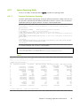
Header:
Version: 2
Flags: little-endian
Header size: 40 bytes
Elapsed time: 9303 us
World size: 4
Number of partitions: 3
Partitions limits: 1000 1000000
num_intsz: 4 bytes (32 bits)
num_volsz: 8 bytes (64 bits)
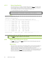
5.1.5.3
Point to Point Communications Section
For point to point communication matrices, use the following. The number of
communication messages is displayed first, then the volume. If either the –-numeric-only or –
-volumic-only options are used then only one matrix is displayed accordingly.
Example
Point to point:
numeric (number of messages)
0
1.1k
0
0 |
1.1k
0
0
0 |
0
0
0
1.1k |
0
0
1.1k
0 |
1.1k
1.1k
1.1k
1.1k
Chapter 5. MPI Application Profiling
29
volumic (Bytes)
0 818.8k
0
0 |
818.8k
0
0
0 |
0
0
0 818.8k |
0
0 818.8k
0 |
818.8k
818.8k
818.8k
818.8k
If the file contains several partitions and the -J/--split option is set then this command
displays as many numeric matrices as there are partitions. Example:
Point to point:
numeric (number of messages)
0 <= msg size < 1000
0
800
0
0 |
800
0
0
0 |
0
0
0
800 |
0
0
800
0 |
800
800
800
800
1000 <= msg size < 1000000
0
300
0
0
300
0
0
0
0
0
0
300
0
0
300
0
|
|
|
|
300
300
300
300
1000000 <= msg size
0
0
0
0
0
0
0
0
0
0
0
0
|
|
|
|
0
0
0
0
volumic (Bytes)
0 818.8k
0
0 |
818.8k
0
0
0 |
0
0
0 818.8k |
0
0 818.8k
0 |
818.8k
818.8k
818.8k
818.8k
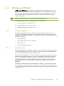
0
0
0
0
If the -r/--rate option is set then the messages rate and data rate matrices are shown
instead of communications matrices. These rates are the average rates for all execution
times not the instantaneous rates. Example:
5.1.5.4
Point to point:
message rate (msg/s)
0 118.2k
0
0 |
118.2k
0
0
0 |
0
0
0 118.2k |
0
0 118.2k
0 |
118.2k
118.2k
118.2k
118.2k
data rate (Bytes/s)
0 88.01M
0
0 |
88.01M
0
0
0 |
0
0
0 88.01M |
0
0 88.01M
0 |
88.01M
88.01M
88.01M
88.01M
Collective Section
The collective section is equivalent to the point-to-point section for collective communication
matrices. Example:
Collective:
numeric (number of messages)
0
102
202
102 |
102
0
0
100 |
202
0
0
0 |
102
100
0
0 |
30
bullx DE User's Guide
406
202
202
202
volumic (Bytes)
0 409.6k 421.6k 409.6k | 1.241M
12.04k
0
0
12k | 24.04k
421.6k
0
0
0 | 421.6k
12.04k 409.6k
0
0 | 421.6k
5.1.5.5
Call table section
This section contains the call table. If the –-ct-total-only option is activated, only the
total column is displayed. Example:
Call table:
Allgather
Allgatherv
Allreduce
Alltoall
Alltoallv
Bcast
Bsend
Gather
Gatherv
Ibsend
Irsend
Isend
Issend
Reduce
Reduce_scatter
Rsend
Scan
Scatter
Scatterv
Send
Sendrecv
Sendrecv_replace
Ssend
Start
5.1.5.6
0
0
0
2
0
0
200
0
0
0
0
0
0
0
200
0
0
0
0
0
1.1k
0
0
0
0
1
0
0
2
0
0
200
0
0
0
0
0
0
0
200
0
0
0
0
0
1.1k
0
0
0
0
2
0
0
2
0
0
200
0
0
0
0
0
0
0
200
0
0
0
0
0
1.1k
0
0
0
0
3
0
0
2
0
0
200
0
0
0
0
0
0
0
200
0
0
0
0
0
1.1k
0
0
0
0
4
0
0
2
0
0
200
0
0
0
0
0
0
0
200
0
0
0
0
0
1.1k
0
0
0
0
5
0
0
2
0
0
200
0
0
0
0
0
0
0
200
0
0
0
0
0
1.1k
0
0
0
0
6
0
0
2
0
0
200
0
0
0
0
0
0
0
200
0
0
0
0
0
1.1k
0
0
0
0
7
0
0
2
0
0
200
0
0
0
0
0
0
0
200
0
0
0
0
0
1.1k
0
0
0
0
Total
0
0
16
0
0
1.6k
0
0
0
0
0
0
0
1.6k
0
0
0
0
0
8.8k
0
0
0
0
Histograms Section
This section contains the message sizes histograms. It shows the number of messages
whose size is zero, between 1 and 9, between 10 and 99, ..., between 108 and 109-1
and greater than 109.
Example:
Histograms of msg sizes
size
pt2pt
coll total
0
0
0
0
1
800
6
806
10
1.2k
6 1.206k
100
1.2k
500
1.7k
1000
1.2k
500
1.7k
104
0
0
0
105
0
0
0
106
0
0
0
107
0
0
0
108
0
0
0
109
0
0
0
Chapter 5. MPI Application Profiling
31
5.1.5.7
Statistics Section
This section displays statistics computed by readpfc. These statistics are based on the
information contained in the data collection file. This section is divided into two or three
sub-sections:
•
The General statistics section contains statistics for the whole application.
•
The Per process average section contains averages per process.
•
The Messages sizes partitions section displays the distribution of messages among the
partitions. This section is only present if there are several partitions.
•
For each statistic we distinguish point to point communications from collective
communications.
Example
General statistics:
Total time: 0.009303s
Messages count |
Volume
|
Avg message size|
Std deviation
|
Variation coef. |
Frequency msg/s |
Throughput B/s |
(0:00:00.009303)
pt2pt |
coll
4400 |
1012
3.2752MB | 2.10822MB
744B | 2.08322kB
1216.4 |
1989.1
1.6341 |
0.95481
472.966k |
108.782k
352.06MB/s | 226.62MB/s
|
total
|
5412
| 5.38342MB
|
995B
|
1488.4
|
1.4963
|
581.748k
| 578.68MB/s
Per process average:
Messages count
Volume
Frequency msg/s
Throughput B/s
pt2pt
|
1100
|
818.8kB
|
118.241k
| 88.015MB/s
|
coll
|
253
| 527.054kB
|
27.1955k
| 56.654MB/s
|
total
|
1353
| 1.34585MB
|
145.437k
| 144.67MB/s
Messages sizes partitions:
|
pt2pt count |
coll count
|
total
count
0 <= sz < 1000
1000 <= sz < 1000000
1000000 <= sz
|
|
|
3.2e+03
1.2e+03
0
73% |
27% |
0% |
5.1e+02
5e+02
0
51% |
49% |
0% |
3.7e+03
1.7e+03
0
The message sizes partitions should be examined first.
Where:
Total time
Total execution time between MPI_Init and MPI_Finalize
Messages count
Number of sent messages
Volume
Volume of sent messages (bytes)
Avg message size Average size of messages (bytes)
32
Std deviation
Standard deviation of messages size
Variation coef.
Variation coefficient of messages size
Frequency msg/s
Average frequency of messages (messages per second)
Throughput B/s
Average throughput for sent messages (bytes per second)
bullx DE User's Guide
69%
31%
0%
5.1.5.8
Topology Section
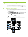
This section shows the distribution of processes on nodes and processors. This distribution is
displayed in two different ways:
First, for each process the node and the CPU in the node where it is running and secondly,
the list of running processes for each node.
Example - 8 Processes Running on 2 Nodes
Topology:
8 process on 2 hosts
process hostid cpuid
0
0
0
1
0
1
2
0
2
3
0
3
4
1
0
5
1
1
6
1
2
7
1
3
host
0
1
5.1.6
processes
0 1 2 3
4 5 6 7
Profilecomm Data Display Options
The following options can be used to display the data:
-a, --all
Displays all the information. Equivalent to –ghimst.
-c, --collective
Displays collective communication matrices.
-g, --topology
Displays the topology of execution environment.
-h, --header
Displays header of the profilecomm file.
-i, --histograms
Displays messages size histograms.
-j, --joined
Displays entire numeric matrices (i.e. not split). This is the default.
-J, --splitted
Display numeric matrices split according to messages size.
-m, --matrix, --matrices
Displays communication matrix (matrices). Equivalent to –cp.
-n, --numeric-only
Does not display volume matrices. This option cannot be used simultaneously with the -v/-volumic-only option.
-p, --p2p, --pt2pt
Displays point to point communication matrices.
Chapter 5. MPI Application Profiling
33
-r, --rate, --throughput
Displays messages rate and data rate matrices instead of communications matrices.
-s, --statistics
Computes and displays some statistics regarding MPI communications.
-S, --scalable
Displays all scalable information; this means all information whose size is independent of
number of processes. Useful when there is a great number of processes. Equivalent to histT.
--square-matrices
Displays the matrices containing the sum of the squared sizes of messages. These matrices
are used for standard deviation computation and are useless for final users. This option is
mainly provided for debugging purposes.
-t, --calltable
Displays the call table.
-T, --ct-total-only
Displays only the Total column of the call table. By default readpfc displays also one
column for each process.
-v, --volumic-only
Does not display numeric matrices. This option cannot be used simultaneously with -n/-numeric-only option.
34
bullx DE User's Guide
5.1.7
Exporting a Matrix or an Histogram
The communication matrices and the histograms can be exported in different formats that
can be used by other software programs, for example spreadsheets. Three formats are
available: CSV (Comma Separated Values), MatrixMarket (not available for histogram
exports) and gnuplot.
It is also possible to have a graphical display of the matrix or the histogram, which is better
for matrices with a large number of elements. Obviously, it is also possible to include the
graphics in a report. Seven graphic formats are available: PostScript, Encapsulated
PostScript, SVG, xfig, EPSLaTeX, PSLaTeX and PSTeX. All these formats are vectorial, which
means the dimensions of the graphics can be modified if necessary.
Figure 5-1.
An example of a communication matrix
Figure 5-2.
An example of a histogram
Chapter 5. MPI Application Profiling
35
5.1.7.1
Options
The following options may be used when exporting matrices:
--csv-separator sep
Modifies CSV delimiter. Default delimiter is comma
“,”. Some software programs prefer a semicolon “;”.
-f format, --format format
Chooses export format. Default format is CSV
(Comma Separated Values).
help
Lists available export formats
csv
Export in CSV format
mm, market, MatrixMarket
Export in MatrixMarket format
gp, gnuplot
Export in a format used by pfcplot so that a
graphical display of the matrix can be produced
ps, postscript
Export in PostScript format
eps
Export in Encapsulated PostScript format
svg
Export in Scalable Vector Graphics format
fig, xfig
Export in xfig format
epslatex
Export in LaTex and Encapsulated PostScript format
pslatex
Export in LaTex format and PostScript inline
pstex
Export in Tex format and PostScript inline
The available values are the following:
mportant
When using epslatex two files are written: xxx.tex and xx.eps. The filename
indicated in the –o option is the name of the Latex file.
--logscale[=base]
Uses a logarithmic color scale. Default value for logarithm basis is 10; this basis can be
modified using the base argument. This option is only relevant when exporting in a
graphical format.
--nogrid
Does not display the grid on a graphical representation of the matrix.
-o file, --output file
Specifies the file name for an export file. The default filenames are out.csv, out.mm, out.dat,
out.ps, out.svg, out.fig or out.tex, according to export format. This option is only available
with the –x option.
--palette pal
Uses a personalized colored palette. This option is only relevant when exporting in a
graphical format. This palette must be compatible with the defined function of gnuplot,
for instance:
--palette '0 "white", 1 "red", 2 "black"' or --palette '0
"#0000ff", 1 "#ffff00", 2 "ff0000"'
--title title
Uses a personalized title for a graphical display. The default title is Point-to-point/collective
numeric/volumic communication matrix, according to the exported matrix.
36
bullx DE User's Guide
-x object, --export object
Exports a communication matrix or histogram specified by the object argument. Values
for object are the following:
help
List of available matrices and histograms
pn[.part],
np[.part]
Point-to-point numeric communication matrix. The optional item part is the
partition number for split matrices. If part is not set, the entire matrix (i.e. the
sum of the split matrices) is exported.
pv, vp
Point to point volumic communication matrix
cn[.part],
Collective numeric communication matrix
nc[.part]
cv, vc
Collective volumic communication matrix
ph, hp
Point-to-point messages size histogram
ch, hc
Collective messages size histogram
th, ht
Total messages size histogram (collective and point-to-point)
ah, ha
Both point-to-point and collective messages size histograms (all histograms)
Other options
-H, --help, --usage Displays help messages
-q, --quiet
Does not display help warning messages (error messages continue to
be displayed).
-V, --version
Displays program version.
Examples
•
To display all information available in foo.pfc file, enter:
$ readpfc -a foo.pfc
This will give information similar to that below
Header:
Version: 2
Flags: little-endian
Header size: 40 bytes
Elapsed time: 9303 us
World size: 4
Number of partitions: 3
Partitions limits: 1000 1000000
num_intsz: 4 bytes (32 bits)
num_volsz: 8 bytes (64 bits)
[...]
Topology:
4 process on 1 hosts
process hostid cpuid
0
0
0
1
0
1
2
0
2
3
0
3
host
0
processes
0 1 2 3
Chapter 5. MPI Application Profiling
37
•
To display a point to point numerical communication matrix:
$ readpfc -pn foo.pfc
Point to point:
numeric (number of messages)
0
1.1k
0
0 |
1.1k
0
0
0 |
0
0
0
1.1k |
0
0
1.1k
0 |
•
1.1k
1.1k
1.1k
1.1k
To export the collective volumic communication matrix in CSV format in the default file:
$ readpfc –x cv foo.pfc
Warning: No output file specified, write to default (out.csv).
$ ls out.csv
out.csv
•
To export the first part (small messages) of point to point numerical communication
matrices in PostScript format in the foo.ps file:
$ readpfc -x np.0 -f ps -o foo.ps foo.pfc
$ ls foo.ps
foo.ps
5.1.7.2
pfcplot, histplot and gnuplot
The pfcplot script converts matrices into graphic using gnuplot. It is generally used by
readpfc, but can be used directly by the user who wants more flexibility. The matrix must
be exported with the –f gnuplot option to be read by pfcplot.
For more details enter:
man pfcplot
Users who have particular requirements can invoke gnuplot directly. To do this the matrix
must be exported with gnuplot format or with CSV format, choosing space as the
separator.
mportant
Due to the limitations of gnuplot, one null line and one null column are added to
the exported matrix in gnuplot format.
Histplot is the equivalent of pfcplot for histograms. Like pfcplot, it can be used directly by
users but it is not user-friendly. More details are available from the man page:
man histplot
38
bullx DE User's Guide
5.2
Scalasca
This section describes how to use the Scalasca performance analysis toolset.
5.2.1
Scalasca Overview
Scalasca (Scalable Performance Analysis of Large-Scale Applications) is an Open-Source
performance-analysis toolset that has been specifically designed for use on large-scale
systems. It is also well adapted for small and medium-scale HPC platforms.
Scalasca supports incremental performance-analysis procedures that integrate runtime
summaries with in-depth studies of concurrent behavior via event tracing, adopting a
strategy of successively refined measurement configurations. A distinctive feature is the
ability to identify wait states that occur, for example, due to unevenly distributed
workloads. Such wait states can lead to poor performance, especially when trying to scale
communication-intensive applications to large processor counts.
The current version of Scalasca supports the performance analysis of applications based on
the MPI, OpenMP, and hybrid programming constructs (OpenMP and hybrid with
restrictions) most widely used in highly scalable HPC applications written in C, C++ and
Fortran on a wide range of current HPC platforms. The user can choose between
generating a summary report (profile) with aggregate performance metrics for individual
function call-paths, and/or generating event traces recording individual runtime events.
Scalasca allows switching between both options to occur, without re-compiling or relinking.
Summarization is particularly useful, as it presents an overview of performance behavior
and of local metrics such as those derived from hardware counters. In addition, it can also
be used to optimize the instrumentation for later trace generation. When tracing is
enabled, each process generates a trace file containing records for all the process local
events.
Following program termination, Scalasca loads the trace files into main memory and
analyzes them in parallel, using as many CPUs as have been used for the target
application itself. During the analysis, Scalasca searches for characteristic patterns
indicating wait states and related performance properties, classifies detected instances by
category and quantifies their significance. The result is a pattern-analysis report similar in
structure to the summary report, but enriched with higher-level communication and
synchronization inefficiency metrics.
Chapter 5. MPI Application Profiling
39
5.2.2
Scalasca Usage
Using Scalasca consists in loading a module file, which will set the different paths for
binaries and libraries.
The Scalasca package provides three module files:
•
scalasca/<version>_bullxmpi -gnu
This module file is to be loaded to use Scalasca with applications compiled with
bullxMPI or any OpenMPI based MPI implementation and using GNU compilers.
•
scalasca/<version>_bullxmpi -intel
This module file is to be loaded to use Scalasca with applications compiled with
bullxMPI or any OpenMPI based MPI implementation and using Intel compilers.
•
scalasca/<version>_intelmpi
This module file is to be loaded to use Scalasca with applications compiled with Intel
MPI and Intel compilers.
To be able to use Scalasca with an application, the first step is to recompile the application
to get it instrumented.
In addition to an almost automatic approach using compiler-inserted instrumentation, semiautomatic POMP and manual instrumentation approaches are also supported.
Manual instrumentation can be used either to augment automatic instrumentation with
region or phase annotations, which can improve the structure of analysis reports – or if
other instrumentations fail.
Once the application instrumented, next steps are execution measurement collection and
analysis, and analysis report examination.
Use the scalasca command with appropriate action flags to instrument application object
files and executables, analyze execution measurements, and interactively examine
measurement/analysis experiment archives:
Note
The PDT-based source-code instrumentation is not supported by this integrated version of
Scalasca.
http://www.vi-hps.org/upload/material/tw11/Scalasca.pdf
5.2.3
More Information
For a full workflow example and more about the application performance analysis, see:
http://www.vi-hps.org/upload/material/tw11/Scalasca.pdf
For more information on Scalasca concepts and projects, see:
http://www.scalasca.org.
40
bullx DE User's Guide
5.3
xPMPI
xPMPI is a framework allowing the use of multiple PMPI tools. PMPI is the MPI profiling
layer defined by the MPI standard to allow the interception of MPI function calls. By
definition, only one tool can intercept a function and forward the call to the real
implementation library. xPMPI is a framework that acts as a PMPI multiplexer by
intercepting the MPI function calls and forwards the call to a chain of patched PMPI tools.
5.3.1
Supported tools
xPMPI allows the combination of the following PMPI tools:
IPM
IPM is a portable profiling tool for parallel codes. It provides a low-overhead performance
profile of the performance aspects and resource utilization in a parallel program.
Communication, computation, and IO are the primary focus.
At the end of a run, IPM dumps a text-based report where aggregate wallclock time,
memory usage and flops are reported along with the percentage of wallclock time spent in
MPI calls, as shown in the following example:
##IPMv0.983########################################################
#
# command : ./TF (completed)
# host : dakar1/x86_64_Linux mpi_tasks : 4 on 1 nodes
# start : 09/14/12/11:28:37 wallclock : 5.381077 sec
# stop : 09/14/12/11:28:42 %comm : 7.15
# gbytes : 9.64523e-01 total gflop/sec : 0.00000e+00 total
#
###################################################################
# region : * [ntasks] = 4
#
# [total] <avg> min max
# entries 4 1 1 1
# wallclock 21.517 5.37924 5.3785 5.38108
# user 25.47 6.3675 6.29 6.44
# system 0.88 0.22 0.16 0.26
# mpi 1.53893 0.384732 0.0103738 0.53211
# %comm 7.14973 0.192783 9.89294
# gflop/sec 0 0 0 0
# gbytes 0.964523 0.241131 0.241112 0.241161
#
#
# [time] [calls] <%mpi> <%wall>
# MPI_Allreduce 0.769333 72 49.99 3.58
# MPI_Send 0.628268 637 40.83 2.92
# MPI_Barrier 0.0887964 432 5.77 0.41
# MPI_Bcast 0.048476 148 3.15 0.23
# MPI_Irecv 0.00139042 563 0.09 0.01
# MPI_Reduce 0.00099695 16 0.06 0.00
# MPI_Wait 0.000902604 560 0.06 0.00
# MPI_Gather 0.000289791 8 0.02 0.00
# MPI_Recv 0.000234257 74 0.02 0.00
# MPI_Comm_size 0.00013079 991 0.01 0.00
# MPI_Waitall 3.91998e-05 1 0.00 0.00
# MPI_Probe 3.63181e-05 3 0.00 0.00
# MPI_Comm_rank 3.54093e-05 232 0.00 0.00
#####################################################################
Chapter 5. MPI Application Profiling
41
Note
In the context of xPMPI, the user applications have not to be recompiled. Hardware
counters profiling is not supported by this integrated version of IPM.
mpiP
mpiP is a lightweight profiling library for MPI applications. Because it only collects
statistical information about MPI functions, mpiP generates considerably less overhead and
much less data than tracing tools. All the information captured by mpiP is task-local. It only
uses communication during report generation, typically at the end of the experiment, to
merge results from all of the tasks into one output file.
Note
In the context of xPMPI, the user applications have not to be recompiled.
At the end of the run, mpiP generates a .mpiP report file in the current directory (default).
We suggest modifying this default to your favorite directory, setting the environment
variable MPIP as follows:
export MPIP="-f /myhome/myfavourite/the_appli"
See http://mpip.sourceforge.net/#mpiP_Output for a complete description of the results.
Should you want to influence the mpiP runtime and customize the generated report, more
options are available with the environment variable MPIP there:
http://mpip.sourceforge.net/#Runtime_Configuration
5.3.2
xPMPI Configuration
The combination of tools can be managed with a configuration file indicating which tools
are activated and their order of execution.
###############################################################
#
# XPMPI configuration file
#
###############################################################
module mpiP
module ipm
The keyword module declares that the tool is activated. The tools are chained in their order
of declaration.
A default configuration file is installed in the following location:
/opt/bullxde/mpicompanions/xPMPI/etc/xpmpi.conf
A user-defined configuration file can be specified with the PNMPI_CONF environment file.
export PNMPI_CONF=<path to user defined configuration file>
5.3.3
xPMPI Usage
Using xPMPI consists in loading a module file. The environment will be set to allow the tool
to intercept MPI functions call without changing the application regular launch process.
Do not forget to unload the module file to disable the use of xPMPI after a profiling session.
42
bullx DE User's Guide
Chapter 6. Analyzing Application Performance
Different tools are available to monitor the performance of your application, and to help
identify problems and to highlight where performance improvements can be made. These
include:
6.1
•
PAPI, an open source tool
•
Bull Performance Monitor (bpmon), a Linux command line single node performance
monitoring tool, which uses the PAPI interface to access the hardware performance
events (counters) of most processors.
•
HPCToolkit, an open source tool based on PAPI and included in the bullx
supercomputer suite delivery.
•
Bull-Enhanced HPCToolkit, based on the current HPCToolkit, it provides added value
for HPC users needing profile based performance analysis in order to optimize their
running software applications
•
Open|SpeedShop an open source multi platform Linux performance tool
PAPI
PAPI (Performance API) is used for the following reasons:
•
•
•
To provide a solid foundation for cross-platform performance analysis tools
To present a set of standard definitions for performance metrics on all platforms
To provide a standard API among users, vendors and academics
PAPI supplies two interfaces:
•
•
A high-level interface, for simple measurements
A low-level interface, programmable, adaptable to specific machines and linking the
measurements
PAPI should only be used by specialists interested in optimizing scientific programs. These
specialists can focus on code sequences using PAPI functions.
PAPI tools are all open source tools.
6.1.1
High-level PAPI Interface
The high-level API provides the ability to start, stop and read the counters for a specified list
of events. It is particularly well designed for programmers who need simple event
measurements, using PAPI preset events.
Compared with the low-level API the high-level is easier to use and requires less setup
(additional calls). However, this ease of use leads to a somewhat higher overhead and the
loss of flexibility.
Note
Earlier versions of the high-level API are not thread safe. This restriction has been removed
with PAPI 3.
Chapter 6. Analyzing Application Performance
43
Below is a simple code example using the high-level API:
#include <papi.h>
#define NUM_FLOPS 10000
#define NUM_EVENTS 1
main()
{
int Events[NUM_EVENTS] = {PAPI_TOT_INS};
long_long values[NUM_EVENTS];
/* Start counting events */
if (PAPI_start_counters(Events, NUM_EVENTS) != PAPI_OK)
handle_error(1);
/* Defined in tests/do_loops.c in the PAPI source distribution */
do_flops(NUM_FLOPS);
/* Read the counters */
if (PAPI_read_counters(values, NUM_EVENTS) != PAPI_OK)
handle_error(1);
printf("After reading the counters: %lld\n",values[0]);
do_flops(NUM_FLOPS);
/* Add the counters */
if (PAPI_accum_counters(values, NUM_EVENTS) != PAPI_OK)
handle_error(1);
printf("After adding the counters: %lld\n", values[0]);
/* double a,b,c; c+= a* b; 10000 times
do_flops(NUM_FLOPS);
*/
/* Stop counting events */
if (PAPI_stop_counters(values, NUM_EVENTS) != PAPI_OK)
handle_error(1);
printf("After stopping the counters: %lld\n", values[0]);
}
Possible Output:
After reading the counters: 441027
After adding the counters: 891959
After stopping the counters: 443994
Note that the second value (after adding the counters) is approximately twice as large as
the first value (after reading the counters). This is because PAPI_read_counters resets and
leaves the counters running, then PAPI_accum_counters adds the current counter value into
the values array.
44
bullx DE User's Guide
6.1.2
Low-level PAPI Interface
The low-level API manages hardware events in user-defined groups called Event Sets. It is
particularly well designed for experienced application programmers and tool developers
who need fine-grained measurements and control of the PAPI interface. Unlike the highlevel interface, it allows both PAPI preset and native event measurements.
The low-level API features the possibility of getting information about the executable and the
hardware, and to set options for multiplexing and overflow handling. Compared with highlevel API, the low-level API increases efficiency and functionality.
An Event Set is a user-defined group of hardware events (preset or native) which, all
together, provide meaningful information. The users specify the events to be added to the
Event Set and attributes such as the counting domain (user or kernel), whether or not the
events are to be multiplexed, and whether the Event Set is to be used for overflow or
profiling. PAPI manages other Event Set settings such as the low-level hardware registers to
use, the most recently read counter values and the Event Set state (running / not running).
Following is a simple code example using the low-level API. It applies the same technique
as the high-level example.
#include <papi.h>
#include <stdio.h>
#define NUM_FLOPS 10000
main()
{
int retval, EventSet=PAPI_NULL;
long_long values[1];
/* Initialize the PAPI library */
retval = PAPI_library_init(PAPI_VER_CURRENT);
if (retval != PAPI_VER_CURRENT) {
fprintf(stderr, "PAPI library init error!\n");
exit(1);
}
/* Create the Event Set */
if (PAPI_create_eventset(&EventSet) != PAPI_OK)
handle_error(1);
/* Add Total Instructions Executed to our Event Set */
if (PAPI_add_event(EventSet, PAPI_TOT_INS) != PAPI_OK)
handle_error(1);
/* Start counting events in the Event Set */
if (PAPI_start(EventSet) != PAPI_OK)
handle_error(1);
/* Defined in tests/do_loops.c in the PAPI source distribution */
do_flops(NUM_FLOPS);
/* Read the counting events in the Event Set */
if (PAPI_read(EventSet, values) != PAPI_OK)
handle_error(1);
printf("After reading the counters: %lld\n",values[0]);
/* Reset the counting events in the Event Set */
if (PAPI_reset(EventSet) != PAPI_OK)
handle_error(1);
do_flops(NUM_FLOPS);
Chapter 6. Analyzing Application Performance
45
/* Add the counters in the Event Set */
if (PAPI_accum(EventSet, values) != PAPI_OK)
handle_error(1);
printf("After adding the counters: %lld\n",values[0]);
do_flops(NUM_FLOPS);
/* Stop the counting of events in the Event Set */
if (PAPI_stop(EventSet, values) != PAPI_OK)
handle_error(1);
printf("After stopping the counters: %lld\n",values[0]);
}
Possible output:
After reading the counters: 440973
After adding the counters: 882256
After stopping the counters: 443913
Note that PAPI_reset is called to reset the counters, because PAPI_read does not reset
the counters. This lets the second value (after adding the counters) to be approximately
twice as large as the first value (after reading the counters).
For more details, please refer to PAPI man and documentation, which are installed with the
product in /usr/share directory.
6.1.3
Collecting FLOP Counts on Sandy Bridge Processors
Floating Point OPerations (FLOP) performance events are very machine type sensitive. The
focus here will be the Sandy Bridge processor. Here are some general insights:
1.
Users think in terms of how many computing operations are done as a count of many
numbers are added, subtracted, compared, multiplied or divided.
2.
Hardware engineers think in terms of how many instructions are done that add,
subtract, compare, multiply or divide.
Three types of operations are provided on these machines:
1. Scalar – One operand per register
2. Packed in 128-bit Register – 4 single precision numbers or 2 double precision numbers
3. Packed in 256-bit Register – 8 single precision numbers or 4 double precision numbers
The FLOP performance events collected by PAPI are influenced by these three types of
operations. The performance events count one for each instruction regardless of the number
of operations done. To compensate for this PAPI has defined several presets that compute
the user expected number of FLOPs by collecting several performance events and
multiplying each one by the proper constant. The PAPI Wiki has a very interesting page
that goes into great detail on this topic:
http://icl.cs.utk.edu/projects/papi/wiki/PAPITopics:SandyFlops
46
bullx DE User's Guide
The PAPI Floating Point Preset Events are as below:
PRESET Event
Description
PAPI_FP_INS
Count of Scalar Operations
PAPI_FP_OPS
same as above
PAPI_SP_OPS
Count of all Single Precision Operations
PAPI_DP_OPS
Count of all Double Precision Operations
PAPI_VEC_SP
Count of all Single Precision Vector Operations
PAPI_VEC_DP
Count of all Double Precision Vector Operations
The following table is from the website. The table shows how single and double precision
operand operations are computed for total operations and for vector operations from the
raw event counts.
PRESET Event
Definition
PAPI_FP_INS
SSE_SCALAR_DOUBLE + SSE_FP_SCALAR_SINGLE
PAPI_FP_OPS
same as above
PAPI_SP_OPS
FP_COMP_OPS_EXE:SSE_FP_SCALAR_SINGLE +
4*(FP_COMP_OPS_EXE:SSE_PACKED_SINGLE) +
8*(SIMD_FP_256:PACKED_SINGLE)
PAPI_DP_OPS
FP_COMP_OPS_EXE:SSE_SCALAR_DOUBLE +
2*(FP_COMP_OPS_EXE:SSE_FP_PACKED_DOUBLE) +
4*(SIMD_FP_256:PACKED_DOUBLE)
PAPI_VEC_SP
4*(FP_COMP_OPS_EXE:SSE_PACKED_SINGLE) +
8*(SIMD_FP_256:PACKED_SINGLE)
PAPI_VEC_DP
2*(FP_COMP_OPS_EXE:SSE_FP_PACKED_DOUBLE) +
4*(SIMD_FP_256:PACKED_DOUBLE))
Chapter 6. Analyzing Application Performance
47
6.2
Bull Performance Monitor (bpmon)
The Bull Performance Monitor tool (bpmon) is a Linux command line single node
performance monitoring tool, which uses the PAPI interface to access the hardware
performance events (counters) of most processors. It is possible to monitor a single thread
or the entire system with bpmon.
The set of events that can be measured depends on the underlying processor. In general,
bpmon gives access to all processor-specific performance events.
bpmon can monitor the performance of the application or the node(s). Command
execution performance can be monitored by bpmon. For example, the command below
gives the following output.
bpmon Syntax
bpmon –e
INSTRUCTIONS_RETIRED,LLC_MISSES,MEM_LOAD_RETIRED:L3_MISS,MEM_UNCORE_RE
TIRED:LOCAL_DRAM,MEM_UNCORE_RETIRED:REMOTE_DRAM
/opt/hpctk/test_cases/llclat -S -l 4 -i 256 -r 200 -o r
Output
Run a single copy of the test on the current thread
Started Timing Reads
Command is <Reads> with Range <200 MB> and Stride <256 B> with Average Time
<63.533 ns>
Elapsed Time of Run of Current Thread is 37.880739086
+-------------------------------------------------------------+
| BPMON Single Thread Event Results
+-------------------------------------------------------------+
Event Description
Event Count
INSTRUCTIONS_RETIRED
10807933019
LLC_MISSES
537361852
MEM_LOAD_RETIRED:L3_MISS
536834525
MEM_UNCORE_RETIRED:LOCAL_DRAM
536834304
MEM_UNCORE_RETIRED:REMOTE_DRAM
67
Elapsed time: 37.893312 seconds
48
bullx DE User's Guide
|
6.2.1
bpmon Reporting Mode
For all, or a subset, of node processors bpmon provides two reporting modes.
6.2.1.1
Processor Performance Reporting
Processor performance reporting lists a set(s) of performance events in tables, with one row
per processor specified and the different performance events in columns. This can be set to
repeat the reporting at regular intervals, as shown in the example below.
#
# Experiment to measure L3 Cache Performance on each Processor without using
Uncore Events
#
# INSTRUCTIONS_RETIRED
measures Total Instructions Executed
# LLC_MISSES
measures L3 Cache Misses
# MEM_LOAD_RETIRED:L3_MISS measures L3 Data Cache Load Misses
# MEM_UNCORE_RETIRED:LOCAL_DRAM measures L3 Data Cache Load Misses Satisfied from
Local DRAM
# MEM_UNCORE_RETIRED:REMOTE_DRAM measures L3 Data Cache Load Misses Satisfied from
Remote DRAM
#
run-time=30
event=INSTRUCTIONS_RETIRED,LLC_MISSES,MEM_LOAD_RETIRED:L3_MISS,MEM_UNCORE_RETIRED:
LOCAL_DRAM,MEM_UNCORE_RETIRED:REMOTE_DRAM
report=event
A command example with its output is shown below.
<Run from Terminal 1> ./llclat -l 10 -c 4
<Run from Terminal 2> sudo bpmon -c
/opt/bullxde/perftools/bpmon/share/doc/bpmon/examples/l3crw
Output
Update in: 30 seconds, ctrl-c to exit
+-------------------------------------------------------------+
| BPMON CPU Event Results |
+-------------------------------------------------------------+
CPU INSTRUCTIONS_RETIRE
LLC_MISSES
MEM_LOAD_RETIRED MEM_UNCORE_RETIRED MEM_UNCORE_RETIRED
#
:L3_MISS
:LOCAL_DRAM
:REMOTE_DRAM
0
11874471347
184298321
181306087
86188440
95116786
1
11864491632
183240206
180310779
83212538
97097821
2
11856905044
183105309
180369962
83542631
96827232
3
11856505436
183098942
180344484
83470335
96873988
4
3292691
5589
1032
367
528
5
401016
2342
466
195
176
6
2594262
981
217
50
121
7
101785
594
150
147
0
8
11848325273
182436818
179645809
83339429
96306262
9
11895706265
182414051
179770963
81956916
97813529
10
11861415833
183430836
180686147
82165023
98520942
11
11867024890
183864157
181035165
84138310
96896833
12
0
0
0
0
0
13
254712
2169
06
138
203
14
388438371
5205
664
286
220
15
6051685
2067
933
839
93
ALL
95325980242 1465907587
1443473264
668015644
775454734
run_time completed. ...bpmon has terminated!!
Chapter 6. Analyzing Application Performance
49
6.2.1.2
Memory Usage Reporting
The second report type is a Memory Utilization Report built into bpmon. This report shows
the percentages of memory references made to a different socket from the one where the
core is executing. This report can also be repeated at a periodic rate.
A command example with its output is shown below.
<Run from Terminal 1> ./llclat -l 10 -c 4
<Run from Terminal 2> sudo bpmon --report memory --run-time 30
Output
Update in: 30 seconds, ctrl-c to exit
+---------------------------------+
| BPMON Memory Utilization Report |
+---------------------------------+
HyperCPU CPU Instruction Memory Read
Local Remote
Board Socket Core Thread CPU Mhz Used Rate (MIPS) Bandwidth(MBPS) Loads Loads
-------------------------------------------------------------------------------------------0
0
0
0
0 2933.3 100.0%
104
515.72 45.8% 54.2%
0
0
1
0
1 2933.3 100.0%
104
516.83 46.0% 54.0%
0
0
2
0
2 2933.3 100.0%
105
521.48 45.4% 54.6%
0
0
3
0
3 2933.3 100.0%
105
519.10 45.6% 54.4%
0
1
0
0
4 1600.1 0.2%
47
0.01 20.4% 79.6%
0
1
1
0
5 1609.1 0.0%
173
0.01 85.9% 14.1%
0
1
2
0
6 1601.1 0.0%
1
0.00 61.9% 38.1%
0
1
3
0
7 1600.8 0.0%
514
0.04 -n/a- -n/a0
0
0
1
8 2933.3 100.0%
104
514.00 45.6% 54.4%
0
0
1
1
9 2933.3 100.0%
106
522.72 45.4% 54.6%
0
0
2
1
10 2933.3 100.0%
105
520.98 45.2% 54.8%
0
0
3
1
11 2933.3 100.0%
104
517.43 45.5% 54.5%
0
1
0
1
12 1613.7 0.0%
0
0.00 -n/a- -n/a0
1
1
1
13 1602.7 0.0%
425
0.01 19.0% 81.0%
0
1
2
1
14 1637.4 0.0%
16
0.00
6.4% 93.6%
0
1
3
1
15 1601.2 0.0%
1492
0.02
92.9% 7.1%
-------------------------------------------------------------------------------------------Totals for 16 CPUs :
36332.1 50.0%
3505
4148.37
45.6% 54.4%
run_time completed. ...bpmon has terminated!!
See
6.2.2
The bpmon man page or help file for more information.
BPMON PAPI CPU Performance Events
The PAPI mechanism used by bpmon enables the review of both PAPI preset events and
processor native events.
PAPI Preset Events
PAPI preset events are the same for all hardware platforms and are derived by addition or
subtraction of native events. However, if the platform processor's native events do not
support the information collection required, then some presets may not exist.
PAPI preset events offer the safest source of information for users who are not expert on the
processor's native events. bpmon allows users to generate a list of available PAPI preset
events, from which the event counts to be used can be chosen.
50
bullx DE User's Guide
PAPI Processor Native Events
bpmon allows the user to generate a list of the processor's native events supported by PAPI.
The user can then review the list and choose which ones to use.
See
6.2.3
Intel64 and IA-32 Architectures Software Developers Manual, Volume 3B: System
Programming Guide, Part 2, (document order number 253669) for details of performance
events available for Intel processors.
BPMON with the Bull Coherent Switch
The Bull Performance Monitor tool (BPMON) includes the ability to report performance
monitor events from the Bull Coherent Switch (BCS). The BCS is the Bull hardware that
interfaces memory traffic between the four mainboard sockets and the next mainboard in
multi-mainboard bullx supernode systems. These performance events provide an insight into
the non-uniform memory architecture (NUMA) related behavior of the system.
The BCS capability is provided by adding a BCS component to the PAPI used with BPMON
and a BCS driver to provide an interface to the BCS hardware performance monitor. The
BCS performance monitor can collect counts for up to four BCS events simultaneously.
Here is an example using the Traffic Identification performance event. Four Incoming Traffic
events are collected, two for Remote memory and two for Local memory:
1.
BCS_PE_REM_Incoming_Traffic[MC=HOM0,MCM=0xF,OC=0,OCM=0xC,NID=1,NI
DM=0x01] counts the number of CPU reads that are satisfied from a Remote node.
2.
BCS_PE_REM_Incoming_Traffic[MC=HOM0,MCM=0xF,OC=RdInvOwn,OCM=0xF,NI
D=1,NIDM=0x01] counts the number of CPU writes that are satisfied from a Remote
node.
3.
BCS_PE_LOM_Incoming_Traffic[MC=HOM0,MCM=0xF,OC=0,OCM=0xC,NID=0,NI
DM=0x18] counts the number of CPU reads that are satisfied from the Local node.
4. BCS_PE_LOM_Incoming_Traffic[MC=HOM0,MCM=0xF,OC=RdInvOwn,OCM=0xF,NI
D=0,NIDM=0x18] counts the number of CPU writes that are satisfied from the Local
node.
Command example
bpmon -e
BCS_PE_REM_Incoming_Traffic[MC=HOM0,MCM=0xF,OC=0,OCM=0xC,NID=1,NIDM=0x01],
BCS_PE_REM_Incoming_Traffic[MC=HOM0,MCM=0xF,OC=RdInvOwn,OCM=0xF,NID=1,NIDM=0x01],
BCS_PE_LOM_Incoming_Traffic[MC=HOM0,MCM=0xF,OC=0,OCM=0xC,NID=0,NIDM=0x18],
BCS_PE_LOM_Incoming_Traffic[MC=HOM0,MCM=0xF,OC=RdInvOwn,OCM=0xF,NID=0,NIDM=0x18]
./llclat -r 200 -l 1 -o r -S
./llclat -r 200 -l 1 -o r -S is the command being measured. This test generates 128M L3
Cache Read Misses. Only this workload must run on the system under test, so that the
measurement results can be related to the workload, as BCS events cannot be limited to a
specific process in the way that the CPU events can.
In this example, REM Incoming Traffic from one BCS should be equal to the LOM Incoming
Traffic from another BCS.
Chapter 6. Analyzing Application Performance
51
The command above gives the following output:
+-------------------------------------------------------------+
| BPMON Single Thread Event Results |
+-------------------------------------------------------------+
Event Description
Event Count
BCS_PE_REM_Incoming_Traffic
448530917
[MC=HOM0,MCM=0xF,OC=0,OCM=0xC,NID=1,NIDM=0x01]
BCS_PE_REM_Incoming_Traffic
483451
[MC=HOM0,MCM=0xF,OC=RdInvOwn,OCM=0xF,NID=1,NIDM=0x01]
BCS_PE_LOM_Incoming_Traffic
448466650
[MC=HOM0,MCM=0xF,OC=0,OCM=0xC,NID=0,NIDM=0x18]
BCS_PE_LOM_Incoming_Traffic
476911
[MC=HOM0,MCM=0xF,OC=RdInvOwn,OCM=0xF,NID=0,NIDM=0x18]
Elapsed time: 76.024967 seconds
52
bullx DE User's Guide
6.3
Open|SpeedShop
This section describes the Open|SpeedShop performance tool.
6.3.1
Open|SpeedShop Overview
Open|SpeedShop is an open source multi-platform Linux performance tool, which is
initially targeted to support performance analysis of applications running on both single
node and large scale IA64, IA32, EM64T, and AMD64 platforms.
Open|SpeedShop is explicitly designed with usability in mind and is for application
developers and computer scientists. The base functionality includes:
•
•
•
•
•
•
Sampling Experiments
Support for Callstack Analysis
Hardware Performance Counters
MPI Profiling and Tracing
I/O Profiling and Tracing
Floating Point Exception Analysis
In addition, Open|SpeedShop is designed to be modular and extensible. It supports
several levels of plug-ins which allow users to add their own performance experiments.
6.3.2
Open|SpeedShop Usage
Using Open|SpeedShop consists in loading a module file, which will set the different paths
for binaries and libraries and some environment variables required for a proper usage.
The Open|SpeedShop package provides two module files:
•
openspeedshop/<version>_bullxmpi
This module file is to be loaded to use Open|SpeedShop with applications compiled
with bullxMPI or any OpenMPI based MPI implementation.
•
openspeedshop/<version>_intelmpi
This module file is to be loaded to use Open|SpeedShop with applications compiled
with Intel MPI.
This integrated version of Open|SpeedShop has been configured to use the offline mode of
operation which links the performance data collection modules with your application and
collects the performance data you specify.
Chapter 6. Analyzing Application Performance
53
6.3.3
More Information
See the documentation available from http://www.openspeedshop.org for more details on
using Open|SpeedShop.
Convenience commands are provided as a very simple syntax and an easier way to invoke
the offline functionality:
http://www.openspeedshop.org/wp/wpcontent/uploads/2013/03/OSSQuickStartGuide2012.pdf
Man pages are available for the Open|SpeedShop invocation command openss and
every convenience script.
Extensive information about how to use the Open|SpeedShop experiments and how to
view the performance information in informative ways is provided here:
http://www.openspeedshop.org/wp/wpcontent/uploads/2013/04/OpenSpeedShop_202_User_Manual_v13.pdf
54
bullx DE User's Guide
6.4
HPCToolkit
HPCToolkit provides a set of profiling tools to help improve the performance of the system.
These tools perform profiling operations on executables and display information in a userfriendly way.
An important advantage of HPCToolkit over other profiling tools is that it does not require
the use of compile-time profiling options or re-linking of the executable.
Note
In this chapter, the term 'executable' refers to a Linux program file, in ELF (Executable and
Linking Format) format.
HPCToolkit is designed to:
6.4.1
•
Work at binary level to ensure language independence
This enables HPCToolkit to support the measurement and analysis of multi-lingual
codes using external binary-only libraries.
•
Profile instead of adding code instrumentation
Sample-based profiling is less intrusive than code instrumentation, and uses a modest
data volume.
•
Collect and correlate multiple performance metrics
Typically, performance problems cannot be diagnosed using only one type of event.
•
Compute derived metrics to help analysis
Derived metrics, such as the bandwidth used for the memory, often provide insights
that will indicate where optimization benefits can be achieved.
•
Attribute costs very precisely
HPCToolkit is unique in its ability to associate measurements in the context of dynamic
calls, loops, and inlined code.
HPCToolkit Workflow
The HPCToolkit design principles led to the development of a general methodology,
resulting in a workflow that is organized around four different capabilities:
•
Measurement of performance metrics during the execution of an application
•
Analysis of application binaries to reveal the program structure
•
Correlation of dynamic performance metrics with the structure of the source code
•
Presentation of performance metrics and associated source code
Chapter 6. Analyzing Application Performance
55
Figure 6-1. HPCToolkit Workflow
As shown in the workflow diagram above, firstly, one compiles and links the application
for a production run, using full optimization. Then, the application is launched with the
hpcrun measurement tool; this uses statistical sampling to produce a performance profile.
Thirdly, hpcstruct is invoked, this tool analyzes the application binaries to recover
information about files, functions, loops, and inlined code. Fourthly, hpcprof is used to
combine performance measurements with information about the program structure to
produce a performance database. Finally, it is possible to examine the performance
database with an interactive viewer, called hpcviewer.
6.4.2
HPCToolkit Tools
The tools included in the HPCToolkit are:
6.4.2.1
hpcrun
hpcrun uses event-based sampling to measure program performance. Sample events
correspond to periodic interrupts induced by an interval timer, or overflow of hardware
performance counters, measuring events such as cycles, instructions executed, cache
misses, and memory bus transactions. During an interrupt, hpcrun attributes samples to
calling contexts to form call path profiles. To accurately measure code from 'black box'
vendor compilers, hpcrun uses on-the-fly binary analysis to enable stack unwinding of fully
optimized code without compiler support, even code that lacks frame pointers and uses
optimizations such as tail calls. hpcrun stores sample counts and their associated calling
contexts in a calling context tree (CCT).
hpcrun-flat, the flat-view version of hpcrun, measures the execution of an executable by a
statistical sampling of the hardware performance counters to create flat profiles. A flat
profile is an IP histogram, where IP is the instruction pointer.
56
bullx DE User's Guide
6.4.2.2
hpcstruct
hpcstruct analyzes the application binary to determine its static program structure. Its goal
is to recover information about procedures, loop nests, and inlined code. For each
procedure in the binary, hpcstruct parses its machine code, identifies branch instructions,
builds a control flow graph, and then uses interval analysis to identify loop nests within the
control flow. It combines this information with compiler generated line map information in a
way that allows HPCToolkit to correlate the samples associated with machine instructions to
the program’s procedures and loops. This correlation is possible even in the presence of
optimizations such as inlining and loop transformations such as fusion, and compilergenerated loops from scalarization of Fortran 90 array operations or array copies induced
by Fortran 90's calling conventions.
6.4.2.3
hpcprof
hpcprof correlates the raw profiling measurements from hpcrun with the source code
abstractions produced by hpcstruct. hpcprof generates high level metrics in the form of a
performance database called the Experiment database, which uses the Experiment XML
format for use with hpcviewer.
hpcprof-flat is the flat-view version of hpcprof and correlates measurements from hpcrun-flat
with the program structure produced by hpcstruct.
hpcproftt correlates flat profile metrics with either source code structure or object code and
generates textual output suitable for a terminal. hpcproftt also generates textual dumps of
profile files.
hpcprof-mpi correlates the call path profiling metrics (in parallel) produced by hpcrun with
the source code structure created by hpcstruct. It produces an Experiment database for use
with the hpcviewer or hpctraceviewer tool. hpcprof-mpi is especially designed for
analyzing and attributing measurements from large-scale executions.
6.4.2.4
hpcviewer
hpcviewer presents the Experiment database produced by hpcprof, hpcprof-flat or hpcprofmpi so that the user can quickly and easily view the performance databases generated.
Chapter 6. Analyzing Application Performance
57
6.4.2.5
Display Counters
The hpcrun tool uses the hardware counters as parameters. To know which counters are
available for your configuration, use the papi_avail command. The hpcrun and hpcrun-flat
tools will also give this information.
papi_avail
Available events and hardware information.
-----------------------------------------------------------------Vendor string and code : GenuineIntel (1)
Model string and code
: 32 (1)
CPU Revision : 0.000000
CPU Megahertz: 1600.000122
CPU's in this Node : 6
Nodes in this System: 1
Total CPU's : 6
Number Hardware Counters : 12
Max Multiplex Counters
: 32
------------------------------------------------------------------
The following correspond to fields in the PAPI_event_info_t structure.
Name
Code Avail Deriv Description (Note)
PAPI_TOT_CYC 0x8000003b Yes No Total cycles
PAPI_L1_DCM0 x80000000 Yes No Level1 data cache misses
PAPI_L1_ICM0 x80000001 Yes No Level 1 instruction cache misses
PAPI_L2_DCM0 x80000002 Yes Yes Level 2 data cache misses
...
PAPI_FSQ_INS 0x80000064 No No Floating point square root instructions
PAPI_FNV_INS 0x80000065 No No Floating point inverse instructions
PAPI_FP_OPS 0x80000066 Yes No Floating point operations
---------------------------------------------------------------------Of 103 possible events, 60 are available, of which 17 are derived.
The following counters are particularly interesting: PAPI_TOT_CYC (number of CPU cycles)
and PAPI_FP_OPS (number of floating point operations).
See
6.4.3
More information about HPCToolkit
See
58
For more information on the display counters, use the papi_avail -d command.
•
The HPCToolkit web at http://www.hpctoolkit.org for more information regarding
HPCToolkit.
•
The HPCToolkit User's Manual, at http://hpctoolkit.org/manual/HPCToolkit-usersmanual.pdf for more detailed information, including Quick Start, FAQ and
Troubleshooting HPCToolkit.
bullx DE User's Guide
6.5
Bull-Enhanced HPCToolkit
Bull-Enhanced HPCToolkit is an application performance profiling tool for HPC users. It is
based on the current HPCToolkit open-source product, which was designed and built by
Rice University, TX, USA. The Bull-Enhanced HPCToolkit provides added value for HPC
users needing profile based performance analysis in order to optimize their running
software applications.
See
Section 6.4 HPCToolkit for more information about the HPCToolkit.
The Bull-Enhanced HPC Toolkit contains three main components:
6.5.1
1.
History Component - see section 6.5.1
2.
Viewing Component - see section 6.5.2
3.
HPCToolkit Wrappers- see section 6.5.3
History Component
The History Component provides a means to store information related to a test run in a
repository. This facility allows the user to keep a history of test runs so that they can be
enhanced with added value, viewed, or compared at a later time. This component consists
of the following parts:
6.5.1.1
•
History Repository
•
History Repository Environment Variables
•
Passport Library
•
Passport Manager Application
History Repository
The History Repository is a database whose entries are code passports from many different
test runs. Each execution of the user's program, which may occur across multiple nodes,
results in one code passport in the History Repository.
Data in the History Repository is stored in a file structure which is grouped first by project
and then by code passports within a project. A code passport contains all of the results
from running a single test including environment information such as compiler version,
compilation platform, surrounding software distributions; program structure information;
and performance information, including raw performance profiles and performance
databases.
A repository name represents a set of data within a repository. This set may be a single
file, many files, or even all of the files in the repository. The fields in a repository name
support glob style pattern matching to provide a friendly way to specify the desired set of
repository files.
Chapter 6. Analyzing Application Performance
59
History Repository naming convention
<repo name> :: <project>:<code passport>:<test tool>:<data origin>:<file path>
<project> :: string
identifies the user or group running test provided by user when bhpcstart is run
<code passport> :: <simple passport>.yyyymmdd.hhmmss
timestamp added when passport created
<simple passport> :: string
identifies application and/or test being run provided by user when bhpcstart is run
<test tool> :: string
name of tool that generated the test results bhpcstruct, bhpcrun, bhpcprof, bhpcprof-mpi
<data origin> :: <system>.<rank>
<system> :: string
system generating test results
<rank> :: string
mpi rank of process generating test results not present if not an mpi job
<file path> :: string
file or directory pathname relative to <data_origin> often just a simple file name
<pathname> :: string
path to a file outside of the repository that may be absolute or relative
6.5.1.2
History Repository Environment Variables
The Bull HPCToolkit extension uses an environment variable to define the location of the
History Repository. The environment variable BHPCTK_REPO_ROOT must be set to the path
name of the repository root. In this release it is a requirement that the repository root path
be locally accessible from all nodes used in the test run.
The environment variable allows multiple repositories on the same system; it also allows
multiple users to share the same repository.
BHPCTK_REPO_ROOT is used by the passport library to locate the History Repository when
applications that use it are run.
6.5.1.3
Passport Library
This library provides an API to manage the History Repository and the information found in
the code passports stored within the repository. The library is responsible for reading the
environment variable BHPCTK_REPO_ROOT to find out where the repository is located.
6.5.1.4
Passport Manager Application
This application is a utility that can be used to access the data in a history repository. Data
in the history repository is stored in a file structure which is grouped first by project and
then by code passports within a project. A code passport contains all of the results from
running a single test.
The Passport Manager tools are accessed with the command bhpcpm.
60
bullx DE User's Guide
Usage
bhpcpm ACTION <repository name> [OPTION [<pathname>]]
A required ACTION field is used to specify the desired function.
An optional OPTION field is used along with the ACTION to achieve the desired result.
Note
Both fields can be entered with a '-' and a single letter or a '--' and a word.
An asterisk '*' is a wild card used for all occurrences of an item.
To display the help information for the Passport Manager Application, enter:
bhpcpm -h
or
bhpcpm –-help
6.5.2
Viewing Component
The enhanced Bull HPCToolkit viewer, bhpcveiwer adds new features to the Rice University
GUI based hpcviewer, which currently displays the contents of the performance database.
New bhpcveiwer features include:
•
Display of the History Repository database
This provides a graphic display of all the files and directories in the history repository
database.
•
Context menu items to perform operations on tree objects
This allows the user to select one or more tree objects and perform some operation on
the objects selected. The kinds of operations to be supported include:
−
Opening files to see contents,
−
Loading an experiment database into the hpcviewer perspective
−
Comparing the content of two selected files in a side by side display that
highlights differences,
−
Comparing all objects in two selected directories to provide a list of the files in
those directories that are different, with the ability to see each file's differences by
opening one of the files in that list.,
−
Import and Export tar files
−
Delete the selected projects and/or code passports
−
Merge Application files and System files
The objective of the merge utility is to create one application or system file for
each bhpcrun/<system_name>.<rank#>/application or system file with the same
content. Files with the same content will be merged into one file and header
information will be added to the merged files to track which process ranks contain
the same content.
•
Preference page to control the History Repository display
This provides controls that affect the History Repository Explorer View.
•
Preference page to control the Grouping Options for the new views
This provides controls that affect the Grouped Metrics View and the Raw Metrics View.
Chapter 6. Analyzing Application Performance
61
•
A Group Metrics view
The idea behind creating the grouped metrics view is that, in any large run some of
the processes will behave differently than other processes. The approach is to
separate the processes into groups of processes which generated similar behavior.
The analyst can decide that one group is running correctly and another running
incorrectly. After doing the grouping the user will have a few sets of processes that
behaved differently from one another. This view only needs to present one set of data
for each group and the analyst only needs to compare the performance differences
between the groups and not all the processes.
•
A Raw Metrics view
This view shows the raw metric values for all of the processes at one program scope.
•
Additional Grouping Features
The grouping tool features include:
•
−
Algorithm to provide an initial optimum number of groups
The grouping mechanism as a default has an algorithm that chooses the optimum
number of groups.
Or the user may specify the number of groups.
−
Automatic hotspot detection
This helps the analyst focus on the program scopes that are of the most value to
analyze and highlights them using different colors that may be chosen by the user.
−
Grouping properties view.
The grouping properties are the results of the grouping tool and principally show
the processes that are part of each group.
Updates to take advantage of information in the performance database
Syntax
To run the enhanced Bull HPCToolkit viewer application, use the bhpcviewer command.
bhpcviewer
See
62
The bhpcviewer application Help menu and then Bull Extensions Manual for more
information about the bhpcviewer.
bullx DE User's Guide
Figure 6-2. bhpcviewer - Bull Extensions Manual page
6.5.3
HPCToolkit Wrappers
Wrapper commands or scripts primary purpose is to run another command or script. They
provide pre- and post-processing as well as support for configuration control of the
arguments of both the wrapper and the script it runs. Often, the input and output files for
the wrappers are obtained from or written to the History Repository.
The bhpcstruct, bhpcrun, bhpcprof and bhpcprof-mpi wrappers can be invoked as CLIs
along with bhpcstart, bhpcstop and bhpcclean.
Command line help
Each of Bull-Enhanced HPCToolkit command-line wrappers will generate a help message
summarizing the tool’s usage, arguments and options.
To display the help information for the wrappers, enter:
<wrapper_name> -h
or
<wrapper_name> –-help
6.5.3.1
Start Component: bhpcstart
When the bhpcstart wrapper is run, it will set the environment used by a test case. A test
case consists of running several scripts, each of which collects some of the data related to
the test. When the test is finished the bhpcstop script should be run.
This wrapper can be used to create a new code passport or to set an existing code
passport to be the current one used by other scripts.
Chapter 6. Analyzing Application Performance
63
•
Creating a new one is accomplished by providing a project name and a simple code
passport name (one without a date/time stamp).
•
Setting an existing code passport to be the current is done by providing the project
name and the full code passport name (including data/time stamp).
Once the bhpcstart script is run, all other scripts that reference the current project and code
passport only require the project name of the repository name.
6.5.3.2
Stop Component: bhpcstop
When the bhpcstop wrapper is run, it will clear the current code passport name for the
input project to stop future scripts from putting more data into this code passport.
6.5.3.3
Clean Component: bhpcclean
When the bhpcclean wrapper is run, it will remove the hpcrun metrics data collected from
a previous run of the bhpcrun script. A user may wish to do this after they create a code
passport and then run the bhpcrun script, if he finds that the bhpcrun used incorrect
parameters or that the wrong versions of software were installed on some of the systems.
A user must run this script before they will be allowed to rerun bhpcrun. This is necessary
because another run of bhpcrun when there is already data collected will cause the test
case to contain invalid data. To be able to present consistent data, all of the information
must have come from the same test run.
6.5.3.4
Compilation Component: bhpcstruct
This component is a wrapper around the HPCToolkit hpcstruct component.
For MPI applications, bhpcstruct must be installed on all possible target nodes where the
test will be executed.
The bhpcstruct wrapper performs these actions:
64
•
Collect special metrics from the program structure to create the program summary
•
Execute the hpcstruct component to create the program structure
•
Collect information to create the program environment
•
Call the Passport Library to write program structure metrics and environment
information to the specified code passport in the designated History Repository
location.
−
The scope tree produced by hpcstruct
<project>.<code passport>.bhpcstruct.<system>.<test case name>.hpcstruct
−
The executable of the test case
<project>.<code passport>.bhpcstruct.<system>.exec.<test case name>
−
Standard Error and Standard Output
<project>.<code passport>.bhpcstruct.<system>.stdout
<project>.<code passport>.bhpcstruct.<system>.stderr
bullx DE User's Guide
6.5.3.5
Parallel Manager Component: bhpcrun
This component is a wrapper around the HPCToolkit hpcrun component.
For MPI applications, bhpcrun must be installed on all possible target nodes where the test
will be executed.
bhpcrun must preserve the node name, process name, and MPI rank (for MPI processes)
used during sample collection to allow tying of abnormal samples back to the node and/or
process on which they occurred.
The bhpcrun wrapper performs these actions:
•
Collect environment information for the system we are running on
•
Collect dynamic libraries used by application
•
Execute the hpcrun component to execute a test case
•
Collect and store the performance profile data generated from a single invocation of
hpcrun on one or more nodes.
•
Call the Passport Library to write the performance profile to the specified code
passport in the designated History Repository location.
−
The performance profile
<project>.<code passport>.bhpcrun.<data origin>.<test case name>-xxx.hpcrun
<project>.<code passport>.bhpcrun.<data origin>.<test case name>-xxx .hpctrace
<project>.<code passport>.bhpcrun.<data origin>.<test case name>-xxx.log
−
The application executable location
<project>.<code passport>.bhpcrun.<data origin>.application
−
The dynamic libraries
<project>.<code passport>.bhpcrun.<data origin>.libraries
−
Standard Error and Standard Output
<project>.<code passport>.bhpcrun.<data origin>.stdout
<project>.<code passport>.bhpcrun.<data origin>.stderr
−
Environment information for the system
<project>.<code passport>.bhpcrun.<data origin>.sys_type
<project>.<code passport>.bhpcrun.<data origin>.variables
The user may also provide optional scripts to perform tasks at specified points during the
execution of the bhpcrun script. The optional prologue script will be executed by bhpcrun
prior to execution of the hpcrun script, and the optional epilogue script will be executed as
the last step in the bhpcrun script. The optional data script will be executed just after the
hpcrun script has completed but prior to the move of the profile data into the History
Repository, allowing the user to manipulate the profile data prior to its insertion. In
addition, a maximum run time value can be provided to limit the execution time of the
bhpcrun test run.
6.5.3.6
Hotplot Component: bhpcprof
This component is a wrapper around the HPCToolkit hpcprof component. It provides an
interface that can be used to add value to a performance database.
The bhpcprof wrapper performs these actions:
Chapter 6. Analyzing Application Performance
65
6.5.3.7
•
Collect the information from the code passport that would normally be used by hpcprof
to build a performance database.
•
Optionally call a user-provided command/script to allow the user to modify the set of
data to be passed to hpcprof.
•
Execute the hpcprof component to build a performance database as an XML file
intended to be displayed by the GUI viewer.
•
Call the Passport Library to write the performance database created by hpcprof to the
specified code passport in the designated History Repository location.
−
The performance database and supporting files
<project>.<code passport>.bhpcprof.<data origin>.perf_db.callpath.xml
<project>.<code passport>.bhpcprof.<data origin>.perf_db.experiment-1.mdb
<project>.<code passport>.bhpcprof.<data origin>.perf_db.experiment.mt
<project>.<code passport>.bhpcprof.<data origin>.perf_db.experiment.xml
−
The performance database source files
<project>.<code passport>.bhpcprof.<data origin>.perf_db.src.xxx
<project>.<code passport>.bhpcprof.<data origin>.perf_db.src.usr.xxx
−
Standard Error and Standard Output
<project>.<code passport>.bhpcprof.<data origin>.stdout
<project>.<code passport>.bhpcprof.<data origin>.stderr
Hotplot Component: bhpcprof-mpi
This component is a wrapper around the HPCToolkit hpcprof-mpi component. It provides an
interface that can be used to add value to a performance database.
The bhpcprof-mpi wrapper performs these actions:
•
Collect the information from the code passport that would normally be used by
hpcprof-mpi to build a performance database.
•
Optionally call a user-provided command/script to allow the user to modify the set of
data to be passed to hpcprof-mpi.
•
Execute the hpcprof-mpi component to build a performance database as an XML file
intended to be displayed by the GUI viewer.
•
Call the Passport Library to write the performance database created by hpcprof-mpi to
the specified code passport in the designated History Repository location.
−
The performance database and supporting files
<project>.<code
<project>.<code
<project>.<code
<project>.<code
66
passport>.bhpcprof-mpi.<data
passport>.bhpcprof-mpi.<data
passport>.bhpcprof-mpi.<data
passport>.bhpcprof-mpi.<data
origin>.perf_db.callpath.xml
origin>.perf_db.experiment-1.mdb
origin>.perf_db.experiment.mt
origin>.perf_db.experiment.xml
−
The performance database source files
<project>.<code passport>.bhpcprof-mpi.<data origin>.perf_db.src.xxx
<project>.<code passport>.bhpcprof-mpi.<data origin>.perf_db.src.usr.xxx
−
Standard Error and Standard Output
<project>.<code passport>.bhpcprof-mpi.<data origin>.stdout
<project>.<code passport>.bhpcprof-mpi.<data origin>.stderr
bullx DE User's Guide
6.5.4
Test Case
Test cases are identified by a project name and code passport name. The project name is
provided by the user running the test as a way to separate his tests from tests run by people
on other projects. It will be provided by the user to all of the scripts run as part of the test
case.
The code passport name represents a single test run by the user. It is possible to run the
same test many times which should create many code passports. When the same test is run
many times, it would be good to be able to recognize that they are all different runs of the
same test. For this reason, the user provides a string to the start script, which will be used to
create a unique code passport name to be used for this test case. The unique name is
created by the passport manager by appending a date/time stamp to the user provided
string.
The passport manager will also keep track of the current code passport (string plus
date/time stamp) being used for each project. This allows scripts run following the
bhpcstart script to get the code passport name being used for the current test from the
passport manager so it does not need to be provided by the user to any other scripts run
for the test case. When the bhpcstop script is run, it will clear the current code passport
name to stop future scripts from putting more data into this code passport. The user needs
to create a new code passport (or set an existing one to be current again) before running
additional scripts.
6.5.4.1
Test run work flow
The work flow is similar to the classical Toolkit, however, the input and output files for the
Toolkit components are obtained from or written to a code passport, as outlined below:
1.
One must initialize the BHPCTK_REPO_ROOT environment variable with the path
name of the History Repository repository root.
2.
One invokes the start component (bhpcstart) with a project name and a simple or full
code passport name. A code passport is created if a partial name is entered and the
last code passport name file is created for the project.
3.
One invokes the compilation component (bhpcstruct), which in turn invokes the classic
hpcstruct tool to perform binary analysis. bhpcstruct writes the program structure to the
code passport.
4.
One launches an application with the parallel manager component (bhpcrun), which
in turn invokes the classic hpcrun tool to execute the binary with statistical sampling.
bhpcrun collects performance profiles from the one or more nodes on which the binary
was executed and adds them to the code passport. It also collects environment
information about the executable on that system. This includes the executables size
and build date plus the environment variables that were set and list of dynamic
libraries used by the executable on that node.
5.
One invokes the hotplot component (bhpcprof or bhpcprof-mpi), which in turn invokes
the classic hpcprof or hpcprof-mpi tool to correlate the performance data with the
source structure, creating a performance database. This database is then added to the
code passport.
6.
One invokes the stop component (bhpcstop) with a project name. The last code
passport name file is deleted for the project.
Chapter 6. Analyzing Application Performance
67
7.
A sample bash script test case to run an MPI MpiSpinWheels job
(/opt/hpctk/test_cases/MpiSpinWheels) is displayed below:
export BHPCTK_REPO_ROOT=/home/hpctk/pmhistrep
bhpcstart -ndemoproj:MpiSpinWheels
bhpcstruct -ndemoproj -T/opt/hpctk/test_cases/MpiSpinWheels
mpirun --mca btl tcp,self -np 8 -x $BHPCTK_REPO_ROOT -host sulu,bones bynode -display-map bhpcrun -ndemoproj -e PAPI_TOT_CYC@1000000 -e
PAPI_TOT_INS@1000000 -H --trace -T/opt/hpctk/test_cases/MpiSpinWheels
mpirun --mca btl tcp,self -np 1 -host bones -x $BHPCTK_REPO_ROOT -bynode
-display-map bhpcprof-mpi -ndemoproj
bhpcstop -ndemoproj
The bhpcviewer Repository Perspective of the code passport
(MpiSpinWheels.20120713.143757) data created by the above example is displayed
below.
Figure 6-3. bhpcviewer Repository page
68
bullx DE User's Guide
6.5.5
HPCToolkit Configuration Files
The enhanced HPCToolkit provides configuration files that are used to control the execution
of each of the components in the package. Each enhanced HPCToolkit component will use
a configuration file named xxx.conf (where xxx is the tool name). It will be possible for a
component's configuration file to appear in one or more of the directories shown below.
The enhanced HPCToolkit components will look for their configuration files in the following
directories (in the order shown):
•
Directory /etc/bullhpctk (to provide system wide default values for tools)
•
Directory $HOME/.bullhpctk (to provide login specific values for tools)
•
Directory in $BHPCTK_CONF_DIR environment variable (to run scripts with custom
configuration files)
Bull will deliver a sample set of configuration files that can be copied into /etc/bullhpctk to
provide system-wide default values for the components delivered with the enhanced
HPCToolkit.
Configuration files contain labels to identify the argument being specified for the
component. In some cases this same label, as well as a single char shortcut for the label,
may be supported as a command line argument to the component.
For each label found in the configuration file, there is a value. This value specifies what the
component uses for this argument. As a component processes each of its configuration files
found in the search path and finds labels, it sets the component's value for this label to the
value found in the configuration file. Therefore, the values found in files later in the search
path normally override the earlier ones.
Configuration files also contain a special label by the name lock. The value for this label is
a comma separated list of the other labels found in this configuration file. When a
component encounters this special label it locks the values provided with each of the labels
in the list. If a label's value has been locked, it prevents the component from replacing it
with a value found in a later configuration file.
Most components also support command line arguments, which follow the same rules
described above for configuration file labels. The values provided on a command line
argument will replace a configuration file value unless it was locked in one of the
configuration files.
The lock directive provides an environment in which administrators can set configuration
values for specific arguments in the /etc/bullhpctk/xxx.conf files that users cannot override
(assuming that users have only read access to the config files in /etc). If a directive is found
that tries to change a locked value, the component prints a warning but continues to run
using the value set prior to when it was locked.
Chapter 6. Analyzing Application Performance
69
6.5.5.1
Compilation Component Configuration File: bhpcstruct.conf
The compilation component uses a configuration file named bhpstruct.conf.
A hypothetical configuration file for this component could look something like this:
#
# User login level configuration for bhpcstruct
#
name democonf
hpcargs "-v 2"
testcase /opt/hpctk/test_cases/MpiSpinWheels
lock testcase
6.5.5.2
Parallel Manager Configuration File: bhpcrun.conf
The parallel manager component uses a configuration file named bhpcrun.conf.
A hypothetical configuration file for this component could look something like this:
#
# User login level configuration for bhpcrun
#
name democonf
events PAPI_TOT_CYC@1000000 PAPI_TOT_INS@1000000
hpcargs "-v 2"
testcase /opt/hpctk/test_cases/MpiSpinWheels
testargs
maxruntime 01:00:00
6.5.5.3
HOTPLOT Configuration File bhpcprof.conf
The hotplot application uses a configuration file named bhpcprof.conf.
A hypothetical configuration file for this component looks something like this:
#
# User login level configuration for bhpcprof
#
name democonf
include /home/hpctk/pmhistrep/<project>/<cpp>/bhpcprof/<data
origin>.perf_db
hpcargs "-v 2"
70
bullx DE User's Guide
Chapter 7. I/O Profiling
This chapter describes I/O profiling tools.
7.1
Iotop
Iotop is a lightweight top-like tool that shows the I/O activity on disk of running processes.
Figure 7-1. I/O activity displayed by Iotop
Please note that Iotop needs root privileges to run.
See
•
The Iotop man page for usage information.
•
http://guichaz.free.fr/iotop/ for more details.
Chapter 7. I/O Profiling
71
7.2
Darshan
Darshan is a scalable HPC I/O characterization tool. It is designed to capture an accurate
picture of application I/O behavior, including properties such as patterns of access within
files, with minimum overhead. Darshan can be used to investigate and tune the I/O
behavior of complex HPC applications. In addition, Darshan’s lightweight design makes it
suitable for full time deployment for workload characterization of large systems.
7.2.1
Darshan Usage
Using Darshan consists in loading a module file, which will set the different paths for
binaries and libraries. Also the user will be reminded to set the DARSHAN_LOGPATH
variable to the directory the Darshan's log files should be located.
Darshan instruments applications via either compile time wrappers for static executables or
dynamic library preloading for dynamic executables.
The Darshan package provides several module files, described below.
•
•
72
The following module files are to be loaded to use Darshan with applications compiled
with bullx MPI or any OpenMPI based MPI implementation and using GNU compilers:
−
darshan/<version>_bullxmpi_gnu_noinst
It is intended to be used with dynamically linked binary and prepend the Darshan
library to the LD_PRELOAD environment variable.
No recompilation is needed for the user application.
−
darshan/<version>_bullxmpi_gnu_inst
It is for use with static executables and needs the application to be recompiled
with provided Darshan wrappers.
The following module files are to be loaded to use Darshan with applications compiled
with bullx MPI or any OpenMPI based MPI implementation and using Intel compilers:
−
darshan/<version>_bullxmpi_intel_noinst
It is intended to be used with dynamically linked binary and prepend the Darshan
library to the LD_PRELOAD environment variable.
No recompilation is needed for the user application. The Intel compilers
environment, followed by the bullxmpi environment must be loaded before
loading this module file. Please use the compilervars.sh script provided by Intel to
load the Intel compilers environment.
−
darshan/<version>_bullxmpi_intel_inst
It is for use with static executables and needs the application to be recompiled
with provided Darshan wrappers.
bullx DE User's Guide
•
7.2.2
The following module files are to be loaded to use Darshan with applications compiled
with Intel MPI:
−
darshan/<version>_intelmpi_noinst
It is intended to be used with dynamically linked binary and prepend the Darshan
library to the LD_PRELOAD environment variable.
No recompilation is needed for the user application. The Intel compilers
environment, followed by the Intel MPI environment must be loaded before
loading this module file. Please use the compilervars.[c]sh script provided by Intel
to load the Intel compilers environment and mpivars.[c]sh to load the Intel MPI
environment.
−
darshan/<version>_intelmpi_inst
It is for use with static executables and needs the application to be recompiled
with provided Darshan wrappers.
Darshan log files
Before using Darshan, the location of the tool generated traces has to be set. This can be
done by setting the DARSHAN_LOGPATH environment variable to an existing location.
export DARSHAN_LOGPATH=/path/to/logs/
7.2.3
Compiling with Darshan
To allow trace generation with Darshan, the MPI application has to be compiled by
replacing the regular MPI compilers with the wrappers provided by the tool. That is,
depending on the module file loaded:
With darshan/<version>_bullxmpi_gnu_inst or darshan/<version>_bullxmpi_intel_inst:
•
mpicc.darshan for C source files.
•
mpiCC.darshan or mpicxx for C++ source files.
•
mpif77.darshan for Fortran 77 source files.
•
mpif90.darshan for the Fortran 90 source files.
With darshan/<version>_intelmpi_inst:
Note
•
mpiicc.darshan for C source files.
•
mpiicpc.darshan for C++ source files.
The MPI environment must be setup prior to use the Darshan wrappers.
Chapter 7. I/O Profiling
73
7.2.4
Analyzing log files with Darshan utilities
Each time a Darshan instrumented application is executed, it will generate a single binary
and portable log file summarizing the I/O activity from that application. This log file is
generated and placed into the directory pointed by the DARSHAN_LOGPATH environment
variable. The log is generated with a name in the following format:
<username>_<binary_name>_<job_ID>_<date>_<unique_ID>_<timing>.darshan.gz
The Darshan package provides a set of tools to help processing and analyzing the log
files.
•
darshan-job-summary.pl
One can generate a graphical summary of the I/O activity for a job by using the
darshan-job-summary.pl graphical summary tool as in the following example.
darshan-job-summary.pl carns_my-app_id114525_7-27-58921_19.darshan.gz
It will generate a multi-page PDF file based on the name of the input file.
•
darshan-parser
This tool generates a full, human readable dump of all information contained in a log
file. The following example essentially converts the contents of the log file into a fully
expanded text file.
darshan-parser <logfile> > ~/job-characterization.txt
See
http://www.mcs.anl.gov/research/projects/darshan/docs/darshan-util.html#_darshan_parser for a
complete description of darshan-parser results.
7.2.5
•
darshan-convert
Converts an existing log file to the newest log format. If the output file has a .bz2
extension, then it will be re-compressed in bz2 format rather than gz format. It also has
command line options for anonymizing personal data and adding metadata
annotation to the log header.
•
darshan-diff
Compares two darshan log files and shows counters that differ.
•
darshan-analyzer
Walks an entire directory tree of Darshan log files and produces a summary of the
types of access methods used in those log files.
•
darshan-logutils*
This is a library rather than an executable, but it provides a C interface for opening
and parsing Darshan log files. This is the recommended method for writing custom
utilities, as darshan-logutils provides a relatively stable interface across different
versions of Darshan and different log formats.
Darshan Limitations
darshan/<version>_intelmpi_noinst and darshan/<version>_intelmpi_inst will not produce
instrumentation for Fortran executables. They only work with C and C++ executables.
74
bullx DE User's Guide
Chapter 8. Libraries and Other Tools
This chapter describes Boost libraries and other tools.
8.1
Boost
Boost is a collection of high quality C++ libraries intended to be widely useful and usable
across a broad spectrum of application. Boost libraries are fully compliant with the C++
standard library and offer means to manipulate efficiently:
•
threads
•
regular expressions
•
filesystem operations
•
smart pointers
•
strings
•
mathematical graphs
•
any many others
Boost contains two types of libraries:
•
header-only libraries
These libraries are fully defined and implemented within C++ header files (hpp files).
Compiling an application with these libraries consists in indicating the compiler where
to find Boost header files with the -I compilation option. In the context of bullx DE,
loading the Boost module will automatically make the Boost header files visible to the
compiler through the CPATH environment variable.
•
shared or static libraries
To compile with these libraries, one has to indicate the compiler where to find the
libraries. In the context of bullx DE, the BOOST_LIB environment variable can be used
to indicate the Boost libraries as shown in the following example.
Compiling with Boost shared or static libraries
g++ source.cpp -L$BOOST_LIB -lboost_xxxx -o executable
See
http://www.boost.org/ for more details.
Chapter 8. Libraries and Other Tools
75
8.2
OTF (Open Trace Format)
OTF is a library used by the tools like Scalasca to generated traces in the OTF format. The
OTF package also contains additional tools to help processing OTF trace files:
See
76
•
otfmerge – converter program of OTF library
•
otfmerge-mpi - MPI version of otfmerge
•
otfaux - append snapshots and statistics to existing OTF traces at given ’break’ time
stamps
•
vtf2ot f - convert VTF3 trace files to OTF format.
•
otf2vtf - convert OTF trace files to VTF format.
•
otfdump - convert OTF traces or parts of it into a human readable, long version .
•
otf(de)compress - compression program for single OTF files.
•
otf-config - shows parameters of the OTF configuration .
•
otfprofile - generates a profile of a trace in Latex or CSV format.
•
otfshrink - creates a new OTF file that only includes specified processes .
•
otfinfo - program to get basic information of a trace.
•
/opt/bullxde/utils/OTF/share/doc/OTF/otftools.pdf documentation on OTF tool
usage.
•
www.tu-dresden.de/zih/otf for more details.
bullx DE User's Guide
8.3
Ptools
Ptools is a collection of tools that help create and manage CPUSETS.
8.3.1
CPUSETs
CPUSETs are lightweight objects in the Linux kernel that enable users to partition their
multiprocessor machine by creating execution areas. A virtualization layer has been added
so it becomes possible to split a machine in terms of CPUs.
The main motivation of this patch is to give the Linux kernel full administration capabilities
concerning CPUs. CPUSETs are rigidly defined, and a process running inside this
predefined area will not be able to run on other parts of the system.
This is useful for:
•
Creating sets of CPUs on a system, and binding applications to them.
•
Providing a way of creating sets of CPUs inside a set of CPUs so that a system
administrator can partition a system among users, and users can further partition their
partition among their applications.
Typical Usage of CPUSETS
•
CPU-bound applications: Many applications (as it is often the case for cluster apps)
used to have a "one process on one processor" policy using sched_setaffinity() to
define this, but what if we have to run several such apps at the same time? One can
do this by creating a CPUSET for each app.
•
Critical applications: processors inside strict areas may not be used by other areas.
Thus, a critical application may be run inside an area with the knowledge that other
processes will not use its CPUs. This means that other applications will not be able to
lower its reactivity. This can be done by creating a CPUSET for the critical application,
and another for all the other tasks.
Bull CPUSETS
CPUSETS are integrated in the standard Linux kernel. However, the Bull kernel includes the
following additional CPUSET features:
Migration
Change on the fly the execution area for a whole set of processes (for example, to
give more resources to a critical application). When you change the CPU list of a
CPUSET all the processes that belong to the CPUSET will be migrated to stay inside the
CPU list, if and as necessary.
Virtualization
Translate the masks of CPUs given to sched_setaffinity() so they stay inside the set of
CPUs. With this mechanism processors are virtualized for the use of sched_setaffinity()
and /proc information. Thus, any former application using this system call to bind
processes to processors will work with virtual CPUs without any change. A new file is
added to each CPUSET, in the CPUSET file system, to allow a CPUSET to be
virtualized, or not.
Chapter 8. Libraries and Other Tools
77
8.3.2
CPUSETs management tools
The ptools package provides a set of tools to help create, manage end delete CPUSETs:
See
78
•
pcreate and pexec to create a CPUSET.
•
pdestroy to destroy a CPUSET.
•
pls to list the existing CPUSETs.
•
pshell to launch a shell within an environment created with pcreate or pexec.
•
pplace and passign to control the placement of processes on CPUs.
The tools man pages for more details on their usage.
bullx DE User's Guide
Appendix A. Performance Monitoring with BCS Counters
The performance monitoring implemented in the BCS chip provides a means for measuring
system performance and detecting bottlenecks caused by hardware or software. This
Appendix describes some of the ways that the Performance Monitoring (PM) resources can
be programmed to obtain some basic measurements.
A.1
Bull Coherent Switch Architecture
To be able to create monitoring experiments the user must have some understanding of the
BCS architecture. The BCS units are:
•
Remote Space Manager (REM) and Local Space Manager (LOM), collectively referred
to as the Protocol Engine (PE).
•
Link Layer QPI/IOH/XQPI (LLCH, LLIH, and LLXH), collectively referred to as LL; Output
Buffering blocks to QPI/IOH/XQPI (OBC, OBI, and OBX) are considered to be part of
the appropriate LL unit for the purposes of Performance Monitoring, collectively
referred to as OB.
•
Non-coherent Manager Unit (NCMH)
•
Route Through IOH-to-QPI/QPI-to-IOH (ROIC and ROCI), collectively referred to as
RO.
Figure A-1 shows a schematic representation of the BCS units with their performance
monitoring blocks and connections.
LLI1
LLI0
LLC0
OBC
PMLL0
PMLL1
LLC1
OBI
OBI
ROIC
ROCI
PMRO0
PMRO1
PMRO0
PMRO1
ReM
OBX
LLX0
PMLL0
PMLL1
OBX
PMPE0
PMPE1
LLX1
PMLL0
PMLL1
OBC
PMLL0
PMLL1
LLC3
PMLL0
PMLL1
OBC
PMLL0
PMLL1
LLC2
PMLL0
PMLL1
LoM
OBC
PMPE0
PMPE1
OBX
LLX2
PMLL0
PMLL1
PMLL0
PMLL1
NCMH
PMNC0
PMNC1
PMCC
Figure A-1. BCS Architecture for performance monitoring blocks and connections
Appendix A. Performance Monitoring with BCS Counters
79
A.2
Performance Monitoring Architecture
Performance Monitoring as supported by BPMON and Bull’s PAPI enhancement is
composed of two parts:
•
event detection
•
event counting
Event detection logic is placed in all major units. Two events can be decoded per cycle in
each block. All events are then centralized in the Performance Monitoring Central Counter
block (PMCC) implemented in the Non Coherent Manager Unit (NCMH). The PMCC
consists of four counters.
Event Detection
Each unit has two blocks containing the Performance Monitoring Event register (PME) which
can be independently programmed to detect and forward different events. These blocks are
named PMxx0 and PMxx1 (where xx is the unit identifier), whose events are referred to as
event0 and event1, respectively. This two block construct allows two similar events in the
same unit to be selected and sent to the counter blocks, for example a target event such as
a directory access with a specific state as one event and a reference event of all directory
read accesses as a second event.
Event Counting
All unit event outputs are collected in the central counter block located in the NCMH unit.
Here the events are selected as inputs to the four counters. Each counter is controlled by a
Performance Monitoring Resource Control and Status register (PMR). Events from PMxx0
are hardwired to the event selection for counter0 of each counter pair; events from PMxx1
are hardwired to the event selection for counter1 of each counter pair. This is important to
keep in mind if one is trying to combine events from different units into one counter.
80
bullx DE User's Guide
A.3
Event Types
This is a general description of event types. Any differences or additions in the units are
addressed in later sections.
1.
Interface – measure BCS internal traffic from the selected unit to a destination unit.
Details about message type are not available at this level of measurement.
2.
Buffer Occupation – measurement of buffer occupation at or greater than a specified
threshold. Used in association with the timer and multiple runs at different thresholds to
make a histogram of occupation.
3.
Errors – measure double and single ECC errors.
4.
Traffic Identification – measure various events in the life of a transaction based on the
traffic direction and the transaction type (message class and opcode) dependent upon
a mask. Incoming and Outgoing directions are with respect to the unit being
monitored.
5.
Latency – measure latency for selected message sequences, often dependent upon a
mask.
PE Event Types
LoM (Local space Manager) is responsible for ensuring coherency for local addresses.
It behaves as a Home Agent on XQPI representing the Home Agents of all the other
modules and as a Caching Agent on QPI representing the Caching Agents of the local
module.
ReM (Remote space Manager) is responsible for ensuring coherency on remote addresses.
It behaves as a Home Agent on QPI representing the Home Agents of all the other modules
and as a Caching Agent on XQPI representing the Caching Agents of the local module.
Protocol Engine (PE) event types are monitored in the PE units, ReM and LoM, by setting
fields in the PMPE0 or PMPE1 PME registers in the selected unit. Each unit consists of four
instances which must have identical settings for their PME registers. For example, if you
have chosen to monitor an event using the PMPE0_PME register in ReM, all four
PMPE0_PME registers in ReM must have the same value. In the cases where only one
instance event is to be used, such as measuring average latency, the event registers should
still be set up the same for all instances, with the counter control registers selecting only one
instance.
The following event types can be monitored in the PE. Descriptive information is in addition
to the general description above.
1.
Interface – measure traffic from a PE block to OB. Can choose either West (Caching
Agent or CA) side or East (Home Agent or HA) side.
2.
Buffer Occupation – the size of the buffer is in parentheses.
3.
Errors – measure directory, Tracker, and Virtual Output FIFO ECC errors.
Appendix A. Performance Monitoring with BCS Counters
81
4.
Traffic Identification – four choices for traffic direction:
a.
Incoming Traffic – incoming traffic can be identified by a mask-enabled Request
or Home Node ID (RHNID) in addition to Transaction Type.
b.
Outgoing Traffic – outgoing traffic can be identified by a mask-enabled
Destination Node ID in addition to Transaction Type.
c.
Tracker Output Traffic – measure responses during Tracker phases Snoop Snoopy
Nodes, Snoop Directory Nodes, and Read Memory for cache-to-cache transfers.
d.
Lookup Response Traffic – directory status during Read Access of IPT (In Process
Table) or SRAM directories. Shared and Exclusive State events can act as
indicators of program affinity.
5.
Transaction Latency – measure latency for Read, Write, or Snoop transactions based
on the opcode dependent upon an opcode mask.
6.
Starvation – measure starvation starts, duration, or number of starved transactions
versus a threshold.
7.
Retry – measure initial retries, all retries, and all transactions that enter the Retry
Detection stage; select between Short (early detection) or Long (detection at end of
pipeline) and one/some/all Retry types.
8.
Directory Access – measure Read and Update accesses to the SRAM directory, or to
both IPT and SRAM. In ReM, the directories comprise the ILD; in LoM, the directories
comprise the ELD.
9.
Directory Levels – measurement of level occupation at or greater than a specific
threshold. Used in association with the timer and multiple runs at different thresholds to
make a histogram of occupation.
10. Twin Lines – measure different types of SRAM Directory Look-ups related to entries that
contain a Twin Line address, defined as a pair of addresses that differ by one specific
address bit (allows for sharing of the directory entry).
A depiction of the 119 bit PMPE_PME register follows. It is shown in 32-bit packets as that
is how it is read and written in Configuration Access mode using the BCS CSR. Field
description details can be found in the PMPE Event Configuration Register Description.
82
bullx DE User's Guide
Traffic Identification
Tracker Output
State
31 30
0
0
Directory
Access
Response Type Received
29
0
0
0
0
0
0
0
0
Directory Active Levels
Event
0
20
0
19
0
0
Threshold
17
0
16
0
0
0
0
12
0
0
0
1
0
0
0
1
0
0
0
0
0
0
0
0
0
x
x
x
x
x
x
x
x
x
x
x
x
x
x
x
x
x
x
x
x
x
x
x
x
x
x
x
1
x
x
x
x
x
1
x
x
x
x
x
1
x
x
x
x
x
1
x
x
x
x
x
1
x
x
x
x
x
1
x
x
x
x
x
x
x
x
x
x
1
x
0 snSnp: snoop Snoopy nodes
1 dnSnp: snoop Directory nodes
0 homeReq: access memory
x
x
1
x
x
x
x
x
x
x
x
1
x
x
x
x
x
x
x
x
1
x
x
x
x
x
x
x
x
x
Twin Lines
Error Monitoring
Event
11 10
0
0
Event
Event
9
7
6
0
0
0
0
0
0
0
0
0
0
0
0
0
0
0
0
0
0 No Event
x
x
x
x
x
x
1 Directory SRAM single ECC error
x
x
x
x
x
1
x Directory SRAM double ECC error
x
x
x
x
1
x
x Directory LOT single ECC error
x
x
x
1
x
x
x Directory DCT single ECC error
x
x
1
x
x
x
x Directory DLIT single ECC error
x
1
x
x
x
x
x Tracker single ECC error
1
x
x
x
x
x
x Virtual Output FIFO single ECC error
0
0
0 No Event
0
0
1 Lookup to Directory SRAM
0
1
0 Lookup miss
0
1
1 Lookup hit with one of the twin lines in non-I state
1
0
0 Lookup hit with both of the twin lines in non-I state
0 No Event
1 The number of active levels is greater than threshold
0 The number of active levels is equal to the threshold
0
0
0 No Event
0
0
1 Directory SRAM update access
0
1
0 Directory SRAM read access
0
1
1 Directory IPT or SRAM update access
1
0
0 Directory IPT or SRAM read access
1
0
1 Transaction elected to access the pipeline
No Event
snSnp or dnSnp
homeReq
Undef
Undef
RspI
DataC_I
RspS
DataC_S/F
RspCnflt
DataC_E/M
RspIWb
RspSWb
RspFwdI
RspFwdS
RspFwdIWb
RspFwdSWb
Traffic Identification
Incoming/Outgoing
Transaction Type Mask:
Node ID:
Transaction Type:
(msgclass+opcode)
(msgclass+opcode)
DNID outgoing;
Direction required for all Traffic ID Events
required for all Traffic ID Events
RHNID incoming
NID Mask
64
42 41
63 62
55 54
47 46
0
0
0
0
0
0
0
0
0
1
1
1
1
0
0
0
0
0
0
0
0
1
1
1
0
1
0
0
1
1
0
1
0
1
1
1
1
1
0
0
0
0
0
0
1
0
0
0
0
1
0
0
1
1
0
0
1
0
1
1
0
0
0
1
1
1
1
1
1
1
Incoming
Outgoing
Tracker Output
Lookup Response
1
1
1
1
1
1
1
0
0
0
0
0
0
0
1
1
1
1 No Event
HOM: Home - Request
HOM: Home - Response & Writes (commands only)
NDR: Non Data Response
SNP: Snoop
NCS: Non Coherent Standard
NCB: Non Coherent Bypass
DRS: Data Response
SPC: Special Control
x
x
x
x
x
x
x
x
x
1 Specific type
0 All types
x
0
1
1
0
0
1
0
0
0
0
1
0
0
0
0
1
0
0
0
0
1
0
0
1
1
Lookup Response
37
0
1
0
1
1
1
Lookup Directory
Status
36
32
0
0
0
0
0
0 No Event
0
0
0
0
x
x
1 Exclusive State
x
x
x Shared State and 3 sharers
x
x
1
x
x Shared State and 2 sharers
x
x
1
x
x
1
x
x
x Shared State and 1 sharers
1
x
x
x
x Invalid State
Specific NID
All NID's
CA (for default configuration)
IOH (for default configuration)
Ubox (for default configuration)
Appendix A. Performance Monitoring with BCS Counters
83
Buffer Occupation
Threshold
Event
Type
95
92 91 90 89
87 86
0
0
0
0
0
0
0
0
0
0
Starvation
Threshold
0
0
0
0
0
Retry
Type
Event
0
0
78 77
0
0
0
75 74
0
0
0
0
0
0
1
0
0
0 ReadReq
0
0
1 Snoop
0
1
0 WSB
0
1
1 WrReq
1
0
0 CmpFwd
1
0
1 PtlCnfList
0 No Event
1 Number of occupied entries is greater than threshold
0 Number of occupied entries is equal to threshold
0
0
0
0
1
0
0
1
1
0
0
1
0
1
0
73
0
0
0
0
0
0
x
x
x
x
x
x
x
x
x
1
x
x
1
x
x
x
x
x
x
1
x
x
x
x
x
1
1
x
x
x
x
1
x
1
x
x
x
1
x
x
1
x
x
1
x
x
x
1
x
1
x
x
x
x
1
1
x
x
x
x
x
No Event
Start of new Starvation mechanism
Starvation mechanism is active
Number of starved transactions at start of mechanism is greater than threshold
Number of starved transactions at start of mechanism is equal to threshold
Transaction Latency
Interface
Buffer Occupation
Buffer Select
Event
Type
Opcode
Opcode Mask
Event
(max size)
Threshold
95
94
93
92
118 117 116 115 114
111 110
107 106 105 104
101 100
96
0
0
0
0
0
0
0
0
0
0
0
0
0
0
0
0
0
0
0
0
0
0
0
0
0
0
0 Write Buffer (8)
0
0
0
1 DCT (256)
0
0
1
0 LOT (256)
0
0
1
1 West TID pool 0 (64)
0
1
0
0 West TID pool 1 (64)
0
1
0
1 West TID pool 2 (64)
0
1
1
0 West TID pool 3 (64)
0
1
1
1 Sum of West TID pools (96)
1
0
0
0 East TID pool (64)
1
0
0
1 East NDR Virtual fifo (276)
1
0 East SNP Virtual fifo (276)
0
1
1
0
1
1 West HOM Virtual fifo (276)
1
1
0
0 West SNP Virtual fifo (276)
1
1
0
1 WSB (16)
0
0 No Event
0 Read Request
0
1 A packet (=1 flit) has been emitted RT-East to OB
0
1 Write Request
1
0 A packet (=1 flit) has been emitted RT-West to OB
0
1
0 Snoop
1
1
1
1 Specific opcode
0
0 No Event
0
0
0
0 All opcodes
0
1 The message selected in the "Type" field has been captured
1
0 The response to the "Type" field message has been received (DataC for Read, Cmp for Write, and last Snp for Snoop)
84
bullx DE User's Guide
Event
67 66 65 64
0
0
0
0
0
0 No Event
0
1 Retry has occurred
1
0 New retry has occurred
1
1 Valid transaction seen in retry detection
Short Retry
1 Impossible lookup
x Atomicity: same/twin address already in pipeline
Long Retry
1 back invalidate refused
x single ECC errors
x full conflict
x partial conflict
x W-TID pool unavailable
x E-TID pool unavailable
x Output channel not available
NCMH Event Types
Non Coherent Manager Unit (NCMH) manages non-coherent transactions through QPI and
XQPI interfaces.
NCMH event types are monitored by setting fields in the PMNC0 or PMNC1 PME
registers.
The following event types can be monitored in NCMH. Descriptive information is in
addition to the general description at the beginning of this section.
1. Interface – measure non-coherent traffic from NC to QPI or XQPI.
2. Buffer Occupation – measure occupation of QPI or XQPI Tracker buffers.
3. Error – measure ECC errors in NC register files.
4. Traffic Identification – two choices for traffic direction, QPI to XQPI and XQPI to QPI.
Traffic identification can be made using the outgoing mask-enabled updated DNID
and the incoming mask-enabled RHNID in addition to Transaction Type.
5. Transaction Latency – measure latency of selected transactions from the QPI or XQPI
tracker.
6. Lock Latency – measure latency of Lock transactions.
A depiction of the 74 bit PMNC_PME register follows. It is shown in 32-bit packets as that
is how it is read and written in Configuration Access mode using the BCS CSR. Field
description details can be found in the PMNC Event Configuration Register Description.
Error
Lock
Latency
Event
Event
Event Sel
31 30 29 28 27 26 25 24
0
0
0
0
0
0
0
0
0
x
1
Transaction Latency
Transaction Type:
(msgclass+opcode)
17 16
0
0
0
0
0
0
0
0
Buffer Occupation
Transaction Type Mask:
(msgclass+opcode)
0
0
0
0
0
1
1
1
0
0
0
1
0 NDR: Non Data Response
0
0
0
1
0
0 NCS: Non Coherent Standard
0 NCB: Non Coherent Bypass
0
1
1
1
0 DRS: Data Response
1
1
0 Select CSI Tracker Buffer
1 Select XCSI Tracker Buffer
0 No Event
0
0
1 Allocation of selected tracker entry has been captured
1
0 Captured tracker entry has been released
0
0 No Event
1 Lock message sent
0
0 Unlock message sent
1
0 No Event
1 NCCX single ECC error
x NCXC single ECC error
1
0
1
0
1
0
1
0
Incoming packet
RHNID
58
63 62
0
0
0
0
0
0
Traffic
Transaction Type:
Incoming RHNID
(msgclass+opcode)
Mask
required for Traffic Events
57
53 52
1
1
1
1
1
0
0
0
0
1
1
0
1
0
Direction
73
0
0
1
0
1
0
1
0
1
0
1
1
1
0
0
1
0
1
0
1
1
0
1
1
1
1 Specific ID
0 All ID's
1
0
0
0
0
Sel
7
8
9
0
0
0
Threshold
Event
0
2
1
0
0
0
0 No Event
0
1 Number of occupied entries is greater than threshold
0
1
0 Number of occupied entries is equal to threshold
0 Select CSI Tracker Buffer
1 Select XCSI Tracker Buffer
1 Specific type
0 All types
0
0
0
0
Interface
Transaction Type Mask:
(msgclass+opcode)
required for Traffic Events
45 44
0
1
0
0
0
0
0
1
1
1
0
0
0
1
1 No Event
1
1
NDR: Non Data Response
NCS: Non Coherent Standard
NCB: Non Coherent Bypass
DRS: Data Response
1
0
1
0
1
0
1
0
0
Error
Sel Event
36 35 34
0
0
0
Event
33 32
0
0
0
0 No Event
1 NCCX double ECC error
x
1
x NCXC double ECC error
0
0 No Event
0
1 A packet has been emitted
1
0 A flit has been emitted
1
1 Lack of credit on a flit waiting to be emitted
0 NCCX to OB
1 NCXC to OB
1 Specific type
0 All types
37
0
Traffic
Outgoing packet
DNID
Outgoing DNID Mask
63
72
68 67
64
0
0
0
0
0
0
0
0
0
1
1
1
1
1 Specific ID
0
0
0
0
0 All ID's
CSI to XCSI
XCSI to CSI
Appendix A. Performance Monitoring with BCS Counters
85
LL and OB Event Types
Link Layer (LL) is the interface between QPI/IOH/XQPI and the Protocol Engines and
Routing Layer of the BCS. Output Buffers (OB) store and route messages from the Protocol
Engines to the Link Layer.
LL event types are monitored in the LL units, LLCH, LLIH and LLXH, by setting fields in the
PMLL0 or PMLL1 PME registers in the selected unit. Each unit consists of multiple instances;
four in LLCH, two in LLIH, three in LLXH. Unlike the PE units, the LL unit instance need not
have identical settings for their PME registers as each instance is connected to a specific
agent. OB Event types are monitored in the appropriate LL unit.
The following event type can be monitored in LL. Descriptive information is in addition to
the general description at the beginning of this section.
Interface – measure OB to LL traffic.
Below is a depiction of the 33 bit PMLL_PME register. It is shown as a 32-bit packets and a
1-bit packet as that is how it is read and written in Configuration Access mode using the
BCS CSR.
32
0
0
0
0
1
1
1
1
1
Interface
Select
31
28
0
0
0
0
1
1
1
0
0
0
0
0
1
1
1
0
0
0
0
1
0
1
1
0
0
1
1
0
1
0
1
0
1
0
1
0
Anticipat
ion
Event
Event
Select
27
25 24 23 22
20 19
0
0
0
0
0
0
0
0
0
0
0
0
0
1
OB
OB
OB
OB
OB
OB
OB
OB
Buffer Occupation
Threshold
0
0
0
0
0
0
0
0
0 No Event
0
0 No Event
0
1 A packet has been emitted
1
0 A packet has been emitted w/ idle latency
1
1 A flit has been emitted
0
0 Flow control (or lack of credit) on a flit waiting to be emitted
to LL flit0
to LL flit1
to LL flit2
to LL flit3
to LL flit0 and flit1
to LL flit2 and flit3
to LL flit0,1,2,3
to LL flit0,1,2,3; VN0 traffic only
0
10
0
Event
9
8
0
0
0
Error Monitoring
Event
7
0
0
0
0
0
0
0
0
0 No Event
0
0
Clock
Correct
Event
2
1
0
0
0
0
0
0 No Event
0 No Event
RO Event Type
Route Through (RO) units are the direct routing path for messages from the two IOH
modules to QPI and between the IOH modules.
RO event type is monitored in the ROIC and ROCI units by setting fields in the PMRO0 or
PMRO1 PME registers in the selected unit. The following event type can be monitored in
RO. Descriptive information is in addition to the general description at the beginning of this
section.
Interface - measure RO-to-OB traffic or ROIC-to-ROCI traffic.
Below is a depiction of the 4 bit PMRO_PME register. Field description details can be
found in the PMRO Event Configuration Register Description.
Interface
Select
Event
3
2
1
0
0
0
0
0
0
0 No Event
0
1 A packet has been emitted
1
0 A flit has been emitted
1
1 Flow control (or lack of credit) on a flit waiting to be emitted
0
0 RO to OB flow0 (2 flits)
0
1 RO to OB flow1 (2 flits)
1
0 RO to OB flow0 and flow1 (4 flits)
1
1 ROIC to ROCI flow0 and flow1 (unused in ROCI)
86
bullx DE User's Guide
A.4
Event Counts and Counter Threshold Comparisons
There are four Performance Monitor Counters comprised of a counter and a data storage
register, the Performance Monitoring Data register (PMD). Counting is enabled by selecting
a Counter Enable source, either a Local Enable/Interval Timer, or the counter's partner. It is
important to note that Local Enable and Interval Timer are controlled by the global registers
PERFCON and PTCTL and are mutually exclusive, meaning that all counters making this
selection will receive the same enable source. For example, one cannot choose Local
Enable for one counter and Interval Timer for another.
Each PMD can be compared with its own Performance Monitoring Compare register
(PMC). There are two comparison modes: maximum compare, and compare then update.
In maximum compare mode, the PMC is loaded with an initial value and a notification
occurs when the PMD reaches this value. In the compare then update mode, the PMC is
loaded each time the PMD exceeds the PMC value.
Each PM Counter is controlled by a Performance Monitoring Resource Control and Status
register (PMR). The fields to carry out the actions described above are listed below.
1.
unit selection for events or no event - select the units whose events are to be monitored,
based upon the unit type (PE, LL, RO).
2.
compare mode or no comparison - select maximum compare, compare then update, or
no comparison mode.
3.
reset source for counter and status - select partner's compare or overflow status,
partner's event, or nothing as the reset.
4.
source of counter events - select PME event, partner's status, or clock.
5.
count mode - count events or clocks after event.
6.
destination of counter status output - select PERFCON or partner.
7.
counter enable source - local (by PERFCON) or timer, partner's status, or disabled.
8.
reset counter and clear status bits.
Using Bull’s tools the user has no capability to use the Interval Timer 0r Compare
mechanisms.
A depiction of the 32-bit PMR register follows. Field description details can be found in the
PMR Configuration Register Description.
Appendix A. Performance Monitoring with BCS Counters
87
Unit
Type
Source
31 30 29
x
0
0
0
0
1
88
28
0
0
0
0
0
0
0
0
Counter and
Counter
Comp. Status Reset
Event
Mode
Source
Source
15 14
20 19 18 17
12
0
0
0
0
0
0
0
0
0
0
0
0
0
0
0
0
0
0
x
1
x
x
x
x
x
x
x
x
x
1
x
x
x
x
x
x
x
x
x
1
x
x
x
x
x
x
x
x
x
1
x
x
x
x
x
x
x
x
x
1
x
x
x
x
x
x
x
x
x
1
x
x
x
x
x
x
x
x
x
1
x
x
x
x
x
x
x
x
x
1
Unit Event Source
1
x
x
x
x
x
x
x
x
0 PE
1 LL
0 RO
bullx DE User's Guide
Count Counter
Mode
Status
11 10
9
8
0
0
0
0
Counter
Status
Output
Source
7
5
0
0
0
Counter
Enable
Source
4
2
0
0
0
1
0
0
0
1 Reset this counter's resources
1 Clear overflow data bit
0
0
0 Counter Disabled
0
0
1 PERFCON/TIMER local count enable
0
1
0 Counter Partner Status
0
0
0 Status reported in PERFCON
0
0
1 Status reported to Counter Partner
1 Overflow status
1 Compare status
0
0 Count events
0
1 Count clocks after event
0
0
0 Unit PME register event
0
0
1 Counter Partner Status
0
1
0 Clock
0 No Reset Source
0
0
0
0
1 Counter Partner's status
0 Counter Partner's incoming event
0
1
0
0 Compare Disabled
0
1 Max compare
1
0 Compare and update PMC if new max
No Event
PE
LL
RO
LLCH 0
ROIC
LOMH 0
LOMH 1
LLCH 1
ROCI
LOMH 2
LLCH 2
LOMH 3
LLCH 3
REMH 0
LLIH 0
REMH 1
LLIH 1
REMH 2
LLXH 0
REMH 3
LLXH 1
NCMH
LLXH 2
A.5
Software Application Supported BCS Monitoring Events
In this section the set of BCS Performance monitoring events is described. Each
performance event is named, the syntax for requesting it is defined, and the abbreviations
of the many fields that must be used by name and the contents of those fields are defined.
The message classes and their opcodes are used as defined in Section A.6. In making this
description of the supported performance monitoring events some simplifications are made.
Therefore if a user only uses this syntax to describe events then not all capability in the BCS
performance monitoring is available.
A list of all performance events is presented here in the order defined in this section. As
defined they collect counts from all the BCSs in the node:
BCS_PE[]
BCS_PE_Error[]
BCS_PE_LOM_Error[]
BCS_PE_REM_Error[]
BCS_PE_Twin_Lines[]
BCS_PE_LOM_Twin_Lines[]
BCS_PE_REM_Twin_Lines[]
BCS_PE_Directory_Active_Levels[]
BCS_PE_LOM_Directory_Active_Levels[]
BCS_PE_REM_Directory_Active_Levels[]
BCS_PE_Directory_Access_Event[]
BCS_PE_LOM_Directory_Access_Event[]
BCS_PE_REM_Directory_Access_Event[]
BCS_PE_Incoming_Traffic[]
BCS_PE_LOM_Incoming_Traffic[]
BCS_PE_REM_Incoming_Traffic[]
BCS_PE_Outgoing_Traffic[]
BCS_PE_LOM_Outgoing_Traffic[]
BCS_PE_REM_Outgoing_Traffic[]
BCS_PE_Tracker_Traffic[]
BCS_PE_LOM_Tracker_Traffic[]
BCS_PE_REM_Tracker_Traffic[]
BCS_PE_Lookup_Traffic[]
BCS_PE_LOM_Lookup_Traffic[]
BCS_PE_REM_Lookup_Traffic[]
BCS_PE_Short_Retry[]
BCS_PE_LOM_Short_Retry[]
BCS_PE_REM_Short_Retry[]
BCS_PE_Long_Retry[]
BCS_PE_LOM_Long_Retry[]
BCS_PE_REM_Long_Retry[]
BCS_PE_Starvation[]
BCS_PE_LOM_Starvation[]
BCS_PE_REM_Starvation[]
BCS_PE_Buffer_Occupation[]
BCS_PE_LOM_Buffer_Occupation[]
BCS_PE_REM_Buffer_Occupation[]
BCS_PE_Interface_RT_East
BCS_PE_LOM_Interface_RT_East
Appendix A. Performance Monitoring with BCS Counters
89
BCS_PE_REM_Interface_RT_East
BCS_PE_Interface_RT_West
BCS_PE_LOM_Interface_RT_West
BCS_PE_REM_Interface_RT_West
BCS_PE_Tx_Request[]
BCS_PE_LOM_Tx_Request[]
BCS_PE_REM_Tx_Request[]
BCS_PE_Tx_Response[]
BCS_PE_LOM_Tx_Response[]
BCS_PE_REM_Tx_Response[]
BCS_NCMH[]
BCS_NCMH_Buffer_Occupation[]
BCS_NCMH_Tx_QPI_Alloc[]
BCS_NCMH_Tx_XQPI_Alloc[]
BCS_NCMH_Tx_QPI_Release[]
BCS_NCMH_Tx_XQPI_Release[]
BCS_NCMH_Lock_Message
BCS_NCMH_Unlock_Message
BCS_NCMH_Lock_Message_Latency
BCS_NCMH_ECC_Error[]
BCS_NCMH_NCCX_OB[]
BCS_NCMH_NCXC_OB[]
BCS_NCMH_QPI_XQPI_Traffic[]
BCS_NCMH_XQPI_QPI_Traffic[]
BCS_LL[]
BCS_LL_Interface[]
BCS_LL_LLCH_Interface[]
BCS_LL_LLIH_Interface[]
BCS_LL_LLXH_Interface[]
BCS_RO[]
BCS_RO_Interface[]
BCS_RO_ROIC_Interface[]
BCS_RO_ROCI_Interface[]
If the counts from all the BCSs are added together then the syntax above is used as shown.
However a special variant of each performance event is allowed that provides the
capability to choose from which BCS the counts for an event will be collected. This is
controlled in the event definition by noting which BCSs will collect counts for this event. It is
noted by the following syntax for each BCS that will collect the count by putting its number
(0, 1, 2, 3) in the event name (up to three of the four BCSs may be listed):
BCS#1#2#3_PE_REM_Incoming_Traffic[]
For example to get the count from BCS0:
BCS0_PE_Incoming_Traffic[MC=DRS,MCM=0xF,OC=0x0,OCM=0x0,
NID=0,NIDM=0]
For example to get the count from BCS1, BCS2 and BCS3:
BCS123_PE_Incoming_Traffic[MC=DRS,MCM=0xF,OC=0x0,OCM=0x0,
NID=0,NIDM=0]
90
bullx DE User's Guide
This can be especially useful in experiments where the performance analyst is evaluating a
test program that is referencing from one BCS to another and wishes to collect separate
counts from the BCS where the CPU is executing the test and from the BCS where the
memory being referenced is located.
PE Event Setup
For PE count events the PMR for the chosen counter for this event should have the following
settings where Unit Event Source can have one of three values:
Counter Enable Source :
Counter Status Output Source :
Count Mode :
Counter Event Source :
Counter and Status Reset Source :
Compare Mode :
Unit Event Source :
Unit Type Source :
local count enable = 001
perfcon = 000
count events = 00
unit pme event = 000
no reset = 000
disabled = 00
LoM0-3 & ReM0-3 = 111111110
PE = 00
The Unit Event Source can have the above value if both LoM0-3 and ReM0-3 are
configured to provide the source of the count. Here are the three choices:
Unit Event Source :
Unit Event Source :
Unit Event Source :
LoM0-3 & ReM0-3 = 111111110
LoM0-3 = 111100000
ReM0-3 = 000011110
The syntax for the expert user that does not wish any software tool help in defining an
event is to provide the PMR and PMPE_PME register contents:
BCS_PE[PMR=0x1FE00004,LOMH=0.0.0x7E0420.0,REMH=0.0.0x7E0420.0]
Error Monitoring
You select the set of errors you wish to monitor. The definition will fill bits 6-0 of PMPE_PME
register. The PMR for the chosen counter for this event should have values shown in the "PE
Event Setup" section with Unit Event Source chosen as LoM0-3 and ReM0-3. For example:
BCS_PE_Error[DSS]
BCS_PE_Error[DSS+DSD]
Bits 6-0 in binary
0000001
0000011
Where the set of errors and their abbreviations are:
Directory SRAM Single ECC Error DSS
Directory SRAM Double ECC Error DSD
Directory LOT Single ECC Error DLS
Directory DCT Single ECC Error DDCS
Directory DLIT Single ECC Error DDLS
Tracker Single ECC Error TRS
Virtual Output FIFO Single ECC Error VOFS
For Unit Event Source chosen as LoM0-3, here is an example:
BCS_PE_LOM_Error[VOFS]
1000000
For Unit Event Source chosen as ReM0-3, here is an example:
BCS_PE_REM_Error[DDLS]
0010000
Appendix A. Performance Monitoring with BCS Counters
91
Twin Lines Monitoring
You select the Event of this type that you want to count. The definition will fill bits 9-7 of
PMPE_PME register. The PMR for the chosen counter for this event should have values
shown in the "PE Event Setup" section with Unit Event Source chosen as LoM0-3 and ReM03. For example:
BCS_PE_Twin_Lines[LDS]
BCS_PE_Twin_Lines[LM]
BCS_PE_Twin_Lines[LHO]
Bits 9-7 in binary
001
010
011
Where the set of events and their abbreviations are:
Lookup to Directory SRAM
Lookup Miss
Lookup Hit with one of the Twin Lines in non-I State
Lookup Hit with both of the Twin Lines in non-I State
For Unit Event Source chosen as LoM0-3, here is an example:
BCS_PE_LOM_Twin_Lines[LM]
LDS
LM
LHO
LHB
010
For Unit Event Source chosen as ReM0-3, here is an example:
BCS_PE_REM_Twin_Lines[LHB]
100
Directory Active Levels Monitoring
You select the Directory Active Levels Threshold (0-31). You select Active Levels Event:
greater than or equal.
The Directory Active Levels Monitoring field is
Threshold
THR
The definition will fill bits 16-10 of PMPE_PME register. The PMR for the chosen counter for
this event should have values shown in the "PE Event Setup" section with Unit Event Source
chosen as LoM0-3 and ReM0-3. For example:
BCS_PE_Directory_Active_Levels[THR>12]
BCS_PE_Directory_Active_Levels[THR=12]
Bits 16-10 in binary
0110001
0110010
For Unit Event Source chosen as LoM0-3, here is an example:
BCS_PE_LOM_Directory_Active_Levels[THR>12
0110001
For Unit Event Source chosen as ReM0-3, here is an example:
BCS_PE_REM_Directory_Active_Levels[THR=12]
0110010
Directory Access Monitoring
You select the directory access type to count. The definition will fill bits 19-17 of
PMPE_PME register. The PMR for the chosen counter for this event should have values
shown in the "PE Event Setup" section with Unit Event Source chosen as LoM0-3 and ReM03. For example:
BCS_PE_Directory_Access_Event[DSU]
BCS_PE_Directory_Access_Event[DIR]
Bits 19-17 in binary
001
100
Where the set of exclusive events and their abbreviations are:
Directory SRAM Update Access
92
bullx DE User's Guide
DSU
Directory SRAM Read Access
Directory IPT or SRAM Update Access
Directory IPT or SRAM Read Access
Transaction Elected to Access the Pipeline
DSR
DIU
DIR
TEA
For Unit Event Source chosen as LoM0-3, here is an example:
BCS_PE_LOM_Directory_Access_Event[TEA]
101
For Unit Event Source chosen as ReM0-3, here is an example:
BCS_PE_REM_Directory_Access_Event[DSR]
010
Incoming Traffic Identification Monitoring
There are four cases of Traffic Identification Events. This is the first. The Traffic Identification
Direction is selected by setting bits (64-63):
Incoming=
Outgoing=
Tracker Output=
Lookup Response=
00
01
10
11
For this case Incoming (00) is chosen. The defaulted fields are:
Lookup Directory Status=
Tracker Output State=
Tracker Output Response Type Received=
00000
00
0000000000
LST
TOS
TOR
The filled fields are:
Direction= 00
Transaction Type MsgClass MC
Transaction Type OpCode OC
Transaction Type MsgClass Mask MCM
Transaction Type OpCode Mask OCM
Node ID (NID) NID
NID Mask NIDM
The definition will fill bits 64-20 of PMPE_PME register. The PMR for the chosen counter for
this event should have values shown in the "PE Event Setup" section with Unit Event Source
chosen as LoM0-3 and ReM0-3. For example:
Bits 64-20 in binary
BCS_PE_Incoming_Traffic[MC=DRS,MCM=0xF,OC=0x0,OCM=0x0, NID=0,NIDM=0]
001110000011110000000000000000000000000000000
This counts DRS transaction types for all opcodes for all RHNIDs
For Unit Event Source chosen as LoM0-3, here is an example:
BCS_PE_LOM_Incoming_Traffic[MC=DRS,MCM=0xF,OC=0x0,OCM=0x0,
NID=0,NIDM=0]
001110000011110000000000000000000000000000000
For Unit Event Source chosen as ReM0-3, here is an example:
BCS_PE_REM_Incoming_Traffic[MC=DRS,MCM=0xF,OC=0x0,OCM=0x0,
NID=0,NIDM=0]
001110000011110000000000000000000000000000000
Appendix A. Performance Monitoring with BCS Counters
93
Outgoing Traffic Identification Monitoring
There are four cases of Traffic Identification Events. For this case Outgoing (01) is chosen.
The defaulted fields are:
Lookup Directory Status=
Tracker Output State=
Tracker Output Response Type Received=
00000
00
0000000000
LST
TOS
TOR
The filled fields are
Direction=
Transaction Type
Transaction Type
Transaction Type
Transaction Type
Node ID (NID)
NID Mask
01
MsgClass
OpCode
MsgClass Mask
OpCode Mask
MC
OC
MCM
OCM
NID
NIDM
The definition will fill bits 64-20 of PMPE_PME register. The PMR for the chosen counter for
this event should have values shown in the "PE Event Setup" section with Unit Event Source
chosen as LoM0-3 and ReM0-3. For example:
Bits 64-20 in binary
BCS_PE_Outgoing_Traffic[MC=DRS,MCM=0xF,OC=0x0,OCM=0x0, NID=0,NIDM=0]
011110000011110000000000000000000000000000000
This counts DRS transaction types for all opcodes for all DNIDs
For Unit Event Source chosen as LoM0-3, here is an example:
BCS_PE_LOM_Outgoing_Traffic[MC=DRS,MCM=0xF,OC=0x0,OCM=0x0,
NID=0,NIDM=0]
001110000011110000000000000000000000000000000
For Unit Event Source chosen as ReM0-3, here is an example:
BCS_PE_REM_Outgoing_Traffic[MC=DRS,MCM=0xF,OC=0x0,OCM=0x0,
NID=0,NIDM=0]
001110000011110000000000000000000000000000000
Tracker Output Traffic Identification Monitoring
There are four cases of Traffic Identification Events. For this case Tracker Output (10) is
chosen. The defaulted fields are:
Node ID (NID)
NID Mask
Lookup Directory Status=
00000
00000
00000
NID
NIDM
LST
The filled fields are:
Direction=
Transaction Type MsgClass
Transaction Type OpCode
Transaction Type MsgClass Mask
Transaction Type OpCode Mask
Tracker Output State=
Tracker Output Response Type Received=
94
bullx DE User's Guide
10
MC
OC
MCM
OCM
TOS
TOR
The definition will fill bits 64-20 of PMPE_PME register. The PMR for the chosen counter for
this event should have values shown in the "PE Event Setup" section with Unit Event Source
chosen as LoM0-3 and ReM0-3. For example:
Bits 64-20 in binary
BCS_PE_Tracker_Traffic[MC=DRS,MCM=0xF,OC=0x0,OCM=0x0,
TOS=dnSnp,TOR=RsplWb+RspSWb]
101110000011110000000000000000000000000000000
This counts DRS transaction types for all opcodes for the selected Tracker Output state.
For Unit Event Source chosen as LoM0-3, here is an example:
BCS_PE_LOM_Tracker_Traffic[MC=DRS,MCM=0xF,OC=0x0,OCM=0x0,
TOS=dnSnp,TOR=RsplWb+RspSWb]
101110000011110000000000000000000000000000000
For Unit Event Source chosen as ReM0-3, here is an example:
BCS_PE_REM_Tracker_Traffic[MC=DRS,MCM=0xF,OC=0x0,OCM=0x0,
TOS=dnSnp,TOR=RsplWb+RspSWb]
101110000011110000000000000000000000000000000
Lookup Response Traffic Identification Monitoring
There are four cases of Traffic Identification Events. For this case Lookup Response (11) is
chosen. The defaulted fields are:
Node ID (NID)
NID Mask
Tracker Output State=
Tracker Output Response Type Received=
00000
00000
00
0000000000
NID
NIDM
TOS
TOR
The filled fields are:
Direction=
Transaction Type MsgClass
Transaction Type OpCode
Transaction Type MsgClass Mask
Transaction Type OpCode Mask
Lookup Directory Status
11
MC
OC
MCM
OCM
LST
The definition will fill bits 64-20 of PMPE_PME register. The PMR for the chosen counter for
this event should have values shown in the "PE Event Setup" section with Unit Event Source
chosen as LoM0-3 and ReM0-3. For example:
Bits 64-20 in binary
BCS_PE_Lookup_Traffic[MC=DRS,MCM=0xF,OC=0x0,OCM=0x0, LST=EXC+1S]
Appendix A. Performance Monitoring with BCS Counters
95
101110000011110000000000000000000000000000000
This counts DRS transaction types for all opcodes for the selected Lookup Directory
Statuses.
Where the set of exclusive Lookup Directory Statuses and their abbreviations are::
Exclusive State
Shared State and 3 Sharers
Shared State and 2 Sharers
Shared State and 1 Sharer
Invalid State
EXC
3S
2S
1S
INV
For Unit Event Source chosen as LoM0-3, here is an example:
BCS_PE_LOM_Lookup_Traffic[MC=DRS,MCM=0xF,OC=0x0,OCM=0x0, LST=EXC+1S]
101110000011110000000000000000000000000000000
For Unit Event Source chosen as ReM0-3, here is an example:
BCS_PE_REM_Lookup_Traffic[MC=DRS,MCM=0xF,OC=0x0,OCM=0x0, LST=EX+1S]
101110000011110000000000000000000000000000000
Retry Monitoring
You select the Retry Event Type. You select Short or Long Retry type. You select the set of
retries that you wish to monitor.
The Retry Monitoring fields are:
Retry Type
Retry Event
TY
EV
The definition will fill bits 74-65 of PMPE_PME register. The PMR for the chosen counter for
this event should have values shown in the "PE Event Setup" section with Unit Event Source
chosen as LoM0-3 and ReM0-3. For example:
Bits 74-65 in binary
BCS_PE_Short_Retry[EV=NEW,TY=ATOM]
0000001010
BCS_PE_Long_Retry[EV=RET,TY=FC+PC]
1000110001
Where the set of exclusive Retry Events and their abbreviations are:
Retry has Occurred
New Retry has Occurred
Valid Transaction Seen in Retry Detection
Where the set of inclusive Short Retry Types and their abbreviations are:
Impossible Lookup
Atomicity: Same/Twin Address already in Pipeline
IMP
ATOM
Where the set of inclusive Long Retry Types and their abbreviations are:
Back Invalidate Refused
Single ECC Errors
Full Conflict
Partial Conflict
W-TID Pool Unavailable
E-TID Pool Unavailable
Output Channel not Available
BIR
SEE
FC
PC
WTID
ETID
OCNA
For Unit Event Source chosen as LoM0-3, here is an example:
BCS_PE_LOM_Short_Retry[EV=NEW,TY=ATOM]
BCS_PE_LOM_Long_Retry[EV=RET,TY=FC+PC]
96
RET
NEW
VAL
bullx DE User's Guide
0000001010
1000110001
For Unit Event Source chosen as ReM0-3, here is an example:
BCS_PE_REM_Short_Retry[EV=NEW,TY=ATOM]
0000001010
BCS_PE_REM_Long_Retry[EV=RET,TY=FC+PC]
1000110001
Starvation Monitoring
You select the Starvation Type. You select Starvation Event. You select Starvation Threshold;
if you choose Event 011 or 100 otherwise it is set to 0.
The Starvation Monitoring fields are:
Starvation Type
TY
Starvation Event
EV
The definition will fill bits 89-75 of PMPE_PME register. The PMR for the chosen counter for
this event should have values shown in the "PE Event Setup" section with Unit Event Source
chosen as LoM0-3 and ReM0-3. For example:
Bits 89-75 in binary
BCS_PE_Starvation[TY=Snoop,EV_ACT]
001000000000010
BCS_PE_Starvation[TY=WrReq,EV_THR>3]
011000000011011
Where the set of exclusive Starvation Events and their abbreviations are:
Start of New Starvation Mechanism
Starvation Mechanism is Active
Threshold Comparison (Including the threshold amount)
EV_STR
EV_ACT
EV_THR
For Unit Event Source chosen as LoM0-3, here is an example:
BCS_PE_LOM_Starvation[TY=WrReq,EV_THR>3]
011000000011011
For Unit Event Source chosen as ReM0-3, here is an example:
BCS_PE_REM_Starvation[TY=WrReq,EV_THR>3]
011000000011011
Buffer Occupation Monitoring
You select the Buffer Select (choose the buffer to monitor). You select comparison Event:
greater than or equal. You select occupation Threshold.
The Buffer Occupation Monitoring fields are:
Buffer Select
Threshold
BUF
THR
The definition will fill bits 104-90 of PMPE_PME register. The PMR for the chosen counter
for this event should have values shown in the "PE Event Setup" section with Unit Event
Source chosen as LoM0-3 and ReM0 3. For example:
Bits 104-90 in binary
BCS_PE_Buffer_Occupation[BUF=WT0,THR>7]
001100000011101
BCS_PE_Buffer_Occupation[BUF=WB,THR=0]
000000000000011
Appendix A. Performance Monitoring with BCS Counters
97
Where the set of exclusive Buffer Names and their abbreviations are:
Write Buffer
DCT
LOT
West TID Pool 0
West TID Pool 1
West TID Pool 2
West TID Pool 3
Sum of West TID Pools
East TID Pool
East NDR Virtual FIFO
East SNP Virtual FIFO
West HOM Virtual FIFO
West SNP Virtual FIFO
WSB
WB
DCT
LOT
WT0
WT1
WT2
WT3
WTA
ETP
ENDR
ESNP
WHOM
WSNP
WSB
For Unit Event Source chosen as LoM0-3, here is an example:
BCS_PE_LOM_Buffer_Occupation[BUF=WT0,THR>7]
001100000011101
For Unit Event Source chosen as ReM0-3, here is an example:
BCS_PE_REM_Buffer_Occupation[BUF=WT0,THR>7]
001100000011101
Interface Monitoring
You select the direction of packet (flit) flow. Then you can count the number of flits emitted.
The definition will fill bits 106-105 of PMPE_PME register. The PMR for the chosen counter
for this event should have values shown in the "PE Event Setup" section with Unit Event
Source chosen as LoM0-3 and ReM0-3, for example:
Bits 106-105 in binary
BCS_PE_Interface_RT_East
01
BCS_PE_Interface_RT_West
10
BCS_PE_Interface_RT_East counts the number of flits that has been emitted RT-East to OB.
BCS_PE_Interface_RT_West counts the number of flits that has been emitted RT-West to OB.
For Unit Event Source chosen as LoM0-3, here is an example:
BCS_PE_LOM_Interface_RT_East
BCS_PE_LOM_Interface_RT_West
01
10
For Unit Event Source chosen as ReM0-3, here is an example:
BCS_PE_REM_Interface_RT_East
BCS_PE_REM_Interface_RT_West
01
10
Transaction Monitoring
You select the Event: Request or Response. You select the Transaction Type. Then you select
the Opcode and Opcode Mask.
The Buffer Occupation Monitoring fields are:
Transaction Type
OpCode
OpCode Mask
TY
OC
OCM
The definition will fill bits 118-107 of PMPE_PME register. The PMR for the chosen counter
for this event should have values shown in the "PE Event Setup" section with Unit Event
Source chosen as LoM0-3 and
ReM0-3. For example:
98
bullx DE User's Guide
Bits 118-107 in binary
BCS_PE_Tx_Request[TY=Write,OC=WbMtoI,OCM=0xF] 010101001111
BCS_PE_Tx_Response[TY=Snoop,OC=SnpInvOwn,OCM=0xF] 101011001111
For Unit Event Source chosen as LoM0-3, here is an example:
BCS_PE_LOM_Tx_Request[TY=Write,OC=WbMtoI,OCM=0xF]
10101001111
BCS_PE_LOM_Tx_Response[TY=Snoop,OC=SnpInvOwn,OCM=0xF] 101011001111
For Unit Event Source chosen as ReM0-3, here is an example:
BCS_PE_REM_Tx_Request[TY=Write,OC=WbMtoI,OCM=0xF]
010101001111
BCS_PE_REM_Tx_Response[TY=Snoop,OC=SnpInvOwn,OCM=0xF] 101011001111
This is setup to count PE Transactions.
Appendix A. Performance Monitoring with BCS Counters
99
NCMH Event Setup
For the NCMH count events the PMR for the chosen counter for this event should have the
following settings:
Counter Enable Source :
local count enable = 001
Counter Status Output Source :
perfcon = 000
Count Mode :
count events = 00
Counter Event Source :
unit pme event = 000
Counter and Status Reset Source :
no reset = 000
Compare Mode :
disabled = 00
Unit Event Source :
ncmh = 000000001
Unit Type Source :
PE = 00
The syntax for the expert user that does not wish any software tool help in defining an
event is to provide the PMR and PMNC_PME register contents:
BCS_NCMH[PMR=0x00100004,NCMH=0.0x7E0420.0]
Buffer Occupation Monitoring
You select the QPI Tracker Buffer or the XQPI Tracker Buffer. You select the Threshold (0 to
63). You select comparison Event: greater than or equal.
The Buffer Occupation Monitoring fields are:
QPI Tracker Buffer QPI_Tracker
XQPI Tracker Buffer XQPI_Tracker
To the field name is appended the comparison event type > or = and the Threshold amount
as shown in the example below.
The definition will fill bits 8-0 of PMNC_PME register. For example:
BCS_NCMH_Buffer_Occupation[QPI_Tracker>31]
BCS_NCMH_Buffer_Occupation[XQPI_Tracker=3]
BCS_NCMH_Buffer_Occupation[QPI_Tracker>0]
Bits 8-0 in binary
001111101
100001101
000000001
The PMR for the chosen counter for this event should have values shown above.
Transaction Monitoring
You select the Event: Allocate or Release. You Select the Buffer: QPI Tracker or XQPI
Tracker. Then you select the Transaction Type Msgclass, Msgclass Mask, Opcode, and
Opcode Mask.
The Buffer Occupation Monitoring fields are
Transaction Type MsgClass MC
Transaction Type OpCode OC
Transaction Type MsgClass Mask MCM
Transaction Type OpCode Mask OCM
The definition will fill bits 27-9 of PMNC_PME register. For example
Bits 27-9 in binary
BCS_NCMH_Tx_QPI_Alloc[MC=DRS,MCM=0xF,OC=0,OCM=0]
0101110111100000000
BCS_NCMH_Tx_XQPI_Alloc[MC=DRS,MCM=0xF,OC=0,OCM=0]
0111110111100000000
100
bullx DE User's Guide
BCS_NCMH_Tx_QPI_Release[MC=DRS,MCM=0xF,OC=0,OCM=0]
1001110111100000000
BCS_NCMH_Tx_XQPI_Release[MC=DRS,MCM=0xF,OC=0,OCM=0]
1011110111100000000
The PMR for the chosen counter for this event should have values shown in the "NCMH
Event Setup" section.
This is setup to count NCMH Transactions.
Lock Monitoring
Two ways are available to use the Lock Latency event:
1. As a counter to count lock messages and / or
2. As a timer to accumulate the time that Locks are closed.
To setup the counter capability you select one of the two counters listed below (the count
results are expected to be the same). The definition will fill bits 29-28 of PMNC_PME
register. For example:
Bits 29-28 in binary
BCS_NCMH_Lock_Message
01
BCS_NCMH_Unlock_Message
10
The PMR for the chosen counter for this event should have values shown in the "NCMH
Event Setup" section.
There are a number of different latency measurements that can be taken in the PE and
NCMH units. A single measurement is taken by counting the number of cycles from a Start
Event to a Stop Event. As a single measurement isn't useful, the average latency is
measured by counting the latencies of all target transactions and dividing that by the
number of target transactions. [The counter definition above is the definition of target
transactions for this example.]
A pair of counters is required to accumulate the total latency time. PAIR0_CNT0 is set up to
create a signal that lasts for the duration of the transaction. The start event of the
transaction (for example Lock sent to NCMH) is the Event Source; the stop event (Unlock
sent to NCMH) is programmed as the Event Source input to the Partner counter and is used
by PAIR0_CNT0 as the reset source. The compare register for this counter is initialized with
one and the compare output is sent to the partner as the Status Output.
Set up the NCMH event registers for a Lock Latency transaction: Event 0 is the Lock, Event1
is the Unlock. The monitoring event is requested by
BCS_NCMH_Lock_Message_Latency
Pair0_PMNC_PME0
BCS_NCMH_Lock_Message
Bits 29-28 in binary
01
Lock Latency Event : Lock message sent = 01
Pair0_PMNC_PME1
BCS_NCMH_Unlock_Message
Bits 29-28 in binary
10
Set up PMCC for the Interval Timer or Local Count Enable method of running the monitor.
Collect the results by reading the counter PMD registers. Note that PAIR0_CNT0 is not read
as it is not interesting.
The PAIR0_CNT0_PMR for this event should have the following settings:
Counter Enable Source : local count enable/timer = 001
Appendix A. Performance Monitoring with BCS Counters
101
Counter Status Output Source : partner = 001
Count Mode : count events = 00
Counter Event Source : unit pme event = 000
Counter and Status Reset Source : partner's incoming event = 010
Compare Mode : max compare = 01
Unit Event Source : ncmh = 000000001
Unit Type Source : PE = 00
The PAIR0_CNT1_PMR for this event should have the following settings:
Counter Enable Source : local count enable/timer = 001
Counter Status Output Source : perfcon = 000
Count Mode : count events = 00
Counter Event Source : partner status = 001
Counter and Status Reset Source : no reset = 000
Compare Mode : disabled = 00
Unit Event Source : same as PAIR0_CNT0_PMR
Unit Type Source : PE = 00
The PAIR0_CNT0_PMC for this event should have the Compare value set to 1.
PAIR0_CNT1 is setup to count cycles for the duration of the transaction, the sum of the
latencies of all target transactions. The partner status, the comparison of the
PAIR0_CNT0_PMD with the value in PMC (=1), is the Event Source. Note that the Unit
Event Source is set up for one of the PE units, but it is not being used as the Counter Event
Source for this counter; it is being used by the partner as a reset source (remember the
hard link between event0/counter0 and event1/counter1).
ECC Error Monitoring
You select the ECC errors you want to count.
The definition will fill bits 33-30 of the PMNC_PME register. For example:
Bits 33-30 in binary
BCS_NCMH_ECC_Error[CXS]
0001
BCS_NCMH_ECC_Error[CXS+XCS]
0011
Where the set of inclusive ECC Error Types and their abbreviations are
QPI to XQPI (NCCX) Single ECC error
XQPI to QPI (NCXC) Single ECC error
QPI to XQPI Double ECC error
XQPI to QPI Double ECC error
CXS
XCS
CXD
XCD
The PMR for the chosen counter for this event should have values shown in the "NCMH
Event Setup" section.
Interface Monitoring
You select QPI or XQPI to Output Buffer (NCCX to OB or NCXC to OB). You select the
Event that you want to count.
The definition will fill bits 36-34 of PMNC_PME register. For example
Bits 36-34 in binary
BCS_NCMH_NCCX_OB[PKT]
001
BCS_NCMH_NCXC_OB[FLT]
110
Where the set of exclusive Interface Events and their abbreviations are
A Packet has been emitted
A Flit has been emitted
Lack of credit on a Flit waiting to be emitted
102
bullx DE User's Guide
PKT
FLT
LOC
The PMR for the chosen counter for this event should have values shown in the "NCMH
Event Setup" section.
Traffic Monitoring
You select direction: QPI to XQPI or XQPI to QPI. You select the destination node ID (DNID)
and its DNID Mask. You select the requestor node ID (RHNID) and its RHNID Mask. You
select Transaction Type and Mask (msgclass + opcode).
The Traffic Monitoring fields are:
Destination Node ID (NID)
Destination NID Mask
Request NID
Request NID Mask
Transaction Type MsgClass
Transaction Type OpCode
Transaction Type MsgClass Mask
Transaction Type OpCode Mask
DNID
DNIDM
RNID
RNIDM
MC
OC
MCM
OCM
The definition will fill bits 73-37 of PMNC_PME register. For example:
Bits 73-37 in binary
BCS_NCMH_QPI_XQPI_Traffic[DNID=0,DNIDM=0,
RNID=0,RNIDM=0,MC=DRS,MCM=0xF,OC=0x0,OCM=0x0]
0000000000000000000001110111100000000
BCS_NCMH_XQPI_QPI_Traffic[DNID=0,DNIDM=0,
RNID=0,RNIDM=0,MC=DRS,MCM=0xF,OC=0x0,OCM=0x0]
1000000000000000000001110111100000000
The PMR for the chosen counter for this event should have values shown in the "NCMH
Event Setup" section.
LL Event Setup
The event interface from most LL blocks in the BCS chip was connected incorrectly making
many of the event selections non-functional. In fact only one remains usable.
For the LL count events the PMR for the chosen counter for this event should have the
following settings where Unit Event Source can have one of four values:
Counter Enable Source :
Counter Status Output Source :
Count Mode :
Counter Event Source :
Counter and Status Reset Source :
Compare Mode :
Unit Event Source :
Unit Type Source :
local count enable = 001
perfcon = 000
count events = 00
unit pme event = 000
no reset = 000
disabled = 00
LLch0-3 & LLih0-1 & LLxh0-2 = 111111111
LL = 01
The Unit Event Source can have the above value if LLch0-3, LLih0-1 and LLxh0-3 are
configured to provide the source of the count. Here are the four choices:
Unit
Unit
Unit
Unit
Event
Event
Event
Event
Source
Source
Source
Source
:
:
:
:
LLch0-3 & LLih0-1 & LLxh0-2
LLch0-3
LLih0-1
LLxh0-2
= 111111111
= 111100000
= 000011000
= 000000111
Appendix A. Performance Monitoring with BCS Counters
103
The syntax for the expert user that does not wish any software tool help in defining an
event is to provide the PMR and PMLL_PME register contents:
BCS_LL[PMR=0x3FF00004,LLCH=0.0x7E0420,LLIH=0.0x7E0420, LLXH=0.0x7E0420]
Interface Monitoring
You select the Select the type of OB to LL traffic needed. You select the Event.
The Interface Monitoring fields are
Interface Select
Interface Event
IS
IE
The definition will fill bits 32-25 of PMLL_PME register. The PMR for the chosen counter for
this event should have values shown in the "LL Event Setup" section with Unit Event Source
chosen as LLch0-3, LLih0-1 and LLxh0-3. For example
Bits 32-25 in binary
BCS_LL_Interface[IS=OL01,IE=FLT]
10001011
Where the set of exclusive Interface Select Types and their abbreviations are:
(X)QPI to LL Flit 0 and 1
(X)QPI to LL Flit 2 and 3
(X)QPI to LL Flit 0, 1, 2 and 3
(X)QPI to LL Flit 0, 1, 2 and 3 and VNO Traffic Only
LL to HD*R
LL to HD*L
LL to HD*L; Snoop Traffic Only
LL to NC Flit 0 and 1
LL to RO Flit 0 and 1
LL to RO Flit 2 and 3
LL to RO Flit 0, 1 ,2 and 3
LLC/I to OBX or LLX to OBC/I_REM Flit 0 and 1
LLC to OBC_LOM
OB to LL Flit 0
OB to LL Flit 1
OB to LL Flit 2
OB to LL Flit 3
OB to LL Flit 0 and 1
OB to LL Flit 2 and 3
OB to LL Flit 0, 1 ,2 and 3
OB to LL Flit 0, 1 ,2 and 3 and VNO Traffic Only
Where the set of exclusive Interface Event Types and their abbreviations are
A Packet has been Emitted
A Packet has been Emitted with Idle Latency
A Flit has been Emitted
Lack or Credit on a Flit Waiting to be Emitted
104
CL01
CL23
CL0123
CLV
LHR
LHL
LSNP
LN01
LR01
LR23
LR0123
LOBX
LOBC
OL0
OL1
OL2
OL3
OL01
OL23
OL0123
OLV
PKT
PIL
FLT
LOC
For Unit Event Source chosen as LLch0-3, here is an example:
BCS_LL_LLCH_Interface[IS=OL01,IE=FLT]
10001011
For Unit Event Source chosen as LLih0-1, here is an example:
BCS_LL_LLIH_Interface[IS=OL01,IE=FLT]
10001011
For Unit Event Source chosen as LLxh0-2, here is an example:
BCS_LL_LLXH_Interface[IS=OL01,IE=FLT]
10001011
bullx DE User's Guide
RO Event Setup
Only internal Interface Traffic is measured.
For the RO count events the PMR for the chosen counter for this event should have the
following settings where Unit Event Source can have one of three values:
Counter Enable Source :
Counter Status Output Source :
Count Mode :
Counter Event Source :
Counter and Status Reset Source :
Compare Mode :
Unit Event Source :
Unit Type Source :
local count enable = 001
perfcon = 000
count events = 00
unit pme event = 000
no reset = 000
disabled = 00
ROIC & ROCI = 110000000
RO = 10
The Unit Event Source can have the above value if both ROIC and ROCI are configured to
provide the source of the count. Here are the three choices:
Unit Event Source :
Unit Event Source :
Unit Event Source :
ROIC & ROCI = 110000000
ROIC = 100000000
ROCI = 010000000
The syntax for the expert user that does not wish any software tool help in defining an
event is to provide the PMR and PMRO_PME register contents:
BCS_RO[PMR=0x58000004,ROIC=2,ROCI=2]
Interface Monitoring
You select the Select of the type of traffic needed. You select the Event.
The Interface Monitoring fields are:
Interface Select
Interface Event
IS
IE
The definition will fill bits 3-0 of PMRO_PME register. The PMR for the chosen counter for
this event should have values shown in the "RO Event Setup" section with Unit Event Source
chosen as ROIC and ROCI. For example:
Bits 3-0 in binary
BCS_RO_Interface[IS=ROB01,IE=LOC]
1011
Where the set of exclusive Interface Select Types and their abbreviations are:
RO to OB Flow 0
RO to OB Flow 1
RO to OB Flow 0 and 1
ROIC to ROCI Flow 0 and 1
ROB0
ROB1
ROB01
ICCI
Where the set of exclusive Interface Event Types and their abbreviations are:
A Packet has been Emitted
A Flit has been Emitted
Lack or Credit on a Flit Waiting to be Emitted
PKT
FLT
LOC
For Unit Event Source chosen as ROIC, here is an example:
BCS_RO_ROIC_Interface[IS=ROB01,IE=LOC]
1011
For Unit Event Source chosen as ROCI, here is an example:
BCS_RO_ROCI_Interface[IS=ROB01,IE=LOC]
Appendix A. Performance Monitoring with BCS Counters
1011
105
A.6
BCS Key Architectural Values
Message Class and Opcode Mapping
Any Opcodes not explicitly defined are reserved for future use. Opcodes listed as
unsupported have been found to be unsupported in the current version of the BCS. Other
Opcodes may also be unsupported; anyone wishing to discover them is directed to the Intel
QPI Protocol Specification. Likewise, a NHM or TWK designation means that the Opcode
is only valid for that platform. Once again, the designation is not exhaustive, the
assumption being that a user who is counting events based upon Opcodes has the
knowledge to be doing so, or access to documentation that would interpret it. Also,
NcMsgB and NcMsgS contain six and ten message types respectively which cannot be
differentiated for performance monitoring.
Message Class
Snoop (SNP /3)
Home Request
(HM / 0)
Home Response
(HOM / 1)
106
bullx DE User's Guide
Name
Message
Class
Encoding
Opcode
SnpCur
0011
0000
SnpCode
0011
0001
SnpData
0011
0010
SnpInvOwn
0011
0100
SnpInvWbMtoI or SnpInvXtoI
0011
0101
SnpInvItoE
0011
1000
PrefetchHint (unsupported)
0011
1111
RdCur
0000
0000
RdCode
0000
0001
RdData
0000
0010
NonSnpRd (unsupported)
0000
0011
RdInvOwn
0000
0100
InvWbMtoI or InvXtoI
0000
0101
EvctCln (NHM)
0000
0110
NonSnpWr (unsupported)
0000
0111
InvItoE
0000
1000
AckCnfltWbI
0000
1001
WbMtoI
0000
1100
WbMtoE
0000
1101
WbMtoS
0000
1110
AckCnflt
0000
1111
RspI
0001
0000
RspS
0001
0001
Message Class
Response Channel Data (DRS / 14)
Response Channel Non Data (NDR / 2)
Name
Message
Class
Encoding
Opcode
RspCnflt
0001
0100
RspCnfltOwn
0001
0110
RspFwd
0001
1000
RspFwdI
0001
1001
RspFwdS
0001
1010
RspFwdIWb
0001
1011
RspFwdSWb
0001
1100
RspIWb
0001
1101
RspSWb
0001
1110
DataC_(FEIMS)
1110
0000
DataNc
1110
0011
DataC_(FEIS)_FrcAckCnflt
1110
0001
DataC_(FEIS)_Cmp
1110
0010
WbiData
1110
0100
WbSData
1110
0101
WbEData
1110
0110
NonSnpWrData (unsupported)
1110
0111
WbIDataPtl
1110
1000
WbEDataPtl
1110
1010
NonSnpWrDataPtl (unsupported)
1110
1011
Gnt_Cmp
0010
0000
Gnt_FrcAckCnflt
0010
0001
Cmp
0010
1000
FrcAckCnflt
0010
1001
Cmp_FwdCode
0010
1010
Cmp_FwdInvOwn
0010
1011
Cmp_FwdInvItoE
0010
1100
CmpD
0010
0100
AbortTO (unsupported)
0010
0101
Appendix A. Performance Monitoring with BCS Counters
107
Message Class
Name
Message
Class
Encoding
Opcode
NcWr
1100
0000
WcWr
1100
0001
NcMsgB
1100
1000
PurgeTC (TKW)
1100
1001
IntLogical (NHM)
1100
1001
1100
1010
1100
1011
NcWrPtl
1100
1100
WcWrPtl
1100
1101
NCP2PB
1100
1110
DebugData
1100
1111
NcRd
0100
0000
IntAck
0100
0001
FERR
0100
0011
NcRdPtl
0100
0100
NcCfgRd
0100
0101
NcLTRd (unsupported)
0100
0110
NcIORd
0100
0111
NcCfgWr
0100
1001
NcLTWr (unsupported)
0100
1010
NcIOWr
0100
1011
NcMsgS
0100
1100
NcP2PS
0100
1101
Non Coherent Bypass
IntPhysical
(NCB /12 )
IntPrioUpd
Non Coherent
Standard
(NCS / 4)
Table A-1.
108
bullx DE User's Guide
Message Class and Opcode Mapping
QPI and XQPI NodeID Maps
The following are the NodeID maps that represent the QPI NodeIDs used by the protocol
internal to the mainboard and the XQPI NodeIDs used by the protocol between
mainboards.
QPI NodeID Map
Component
NHM 0
NHM 1
NHM 2
NHM 3
Agent
NID
CA0/ HA0
00001
Ubox
00010
CA1/HA1
00011
CA0/ HA0
00101
Ubox
00110
CA1/HA1
00111
CA0/ HA0
01001
Ubox
01010
CA1/HA1
01011
CA0/ HA0
01101
Ubox
01110
CA1/HA1
01111
IOH 0
00000
IOH 1
00100
BCS
Table A-2.
CA0/HA0
10001
NCM
10010
CA1/HA1
10011
HA2
10101
HA3
10111
QPI NodeID Map
Appendix A. Performance Monitoring with BCS Counters
109
XQPI NodeID Map
Component
BCS 0
BCS 1
BCS 2
BCS 3
Table A-3.
110
bullx DE User's Guide
Agent
NID
CA0/HA0
00000
CA1/HA1
00001
NCM
00010
CA2/HA2
00011
CA3/HA3
00100
CA0/HA0
01000
CA1/HA1
01001
NCM
01010
CA2/HA2
01011
CA3/HA3
01100
CA0/HA0
10000
CA1/HA1
10001
NCM
10010
CA2/HA2
10011
CA3/HA3
10100
CA0/HA0
11000
CA1/HA1
11001
NCM
11010
CA2/HA2
11011
CA3/HA3
11100
XQPI NodeID Map
A.7
Configuration Management Description
Performance Monitor Configuration Registers
Register Symbolic
Name
Real Address
CSR
Attribute
Address
Function
Description
for BCS=0/1/2/3,
n=0/2/4/6
Registers that should be initialized
PERFCON
0000_FDnC_5000 3_1400
RW
Control and status
Counter control and Status
PTCTL
0000_FDnC_5004 3_1401
RW
Control and status
Interval timer control and Status
PAIR0_CNT0_PMR 0000_FDnC_5018 3_1406
[31:0]
RW
Control and status
Pair0 Counter0 resource control and
status
PAIR0_CNT1_PMR 0000_FDnC_502C 3_140B
[31:0]
RW
Control and status
Pair0 Counter1 resource control and
status
PAIR1_CNT0_PMR 0000_FDnC_5040 3_1410
[31:0]
RW
Control and status
Pair1 Counter0 resource control and
status
PAIR1_CNT1_PMR 0000_FDnC_5054 3_1415
[31:0]
RW
Control and status
Pair1 Counter1 resource control and
status
PMINIT [31:0]
0000_FDnC_5008 3_1402
RW
Initial value
Initial value of timer, low order bits
PMINIT [44:32]
0000_FDnC_500C 3_1403
RW
Initial value
Initial value of timer, high order bits
Registers that can be initialized,
depending on usage
PAIR0_CNT0_PMC 0000_FDnC_501C 3_1407
[31:0]
RW
Initial or current value Pair0 Counter0 compare value or max
count, low order bits
PAIR0_CNT0_PMC 0000_FDnC_5020 3_1408
[44:32]
RW
Initial or current value Pair0 Counter0 compare value or max
count, high order bits
PAIR0_CNT1_PMC 0000_FDnC_5030 3_140C
[31:0]
RW
Initial or current value Pair0 Counter1 compare value or max
count, low order bits
PAIR0_CNT1_PMC 0000_FDnC_5034 3_140D
[44:32]
RW
Initial or current value Pair0 Counter1 compare value or max
count, high order bits
PAIR1_CNT0_PMC 0000_FDnC_5044 3_1411
[31:0]
RW
Initial or current value Pair1 Counter0 compare value or max
count, low order bits
PAIR1_CNT0_PMC 0000_FDnC_5048 3_1412
[44:32]
RW
Initial or current value Pair1 Counter0 compare value or max
count, high order bits
PAIR1_CNT1_PMC 0000_FDnC_5058 3_1416
[31:0]
RW
Initial or current value Pair1 Counter1 compare value or max
count, low order bits
PAIR1_CNT1_PMC 0000_FDnC_505C 3_1417
[44:32]
RW
Initial or current value Pair1 Counter1 compare value or max
count, high order bits
Registers that are read and can be
cleared
PAIR0_CNT0_PMD 0000_FDnC_5024 3_1409
[31:0]
RW
Current value
Pair0 Counter0 current count, low order
bits
PAIR0_CNT0_PMD 0000_FDnC_5028 3_140A
[44:32]
RW
Current value
Pair0 Counter0 current count, high order
bits
PAIR0_CNT1_PMD 0000_FDnC_5038 3_140E
RW
Current value
Pair0 Counter1 current count, low order
Appendix A. Performance Monitoring with BCS Counters
111
Register Symbolic
Name
Real Address
CSR
Attribute
Address
Function
Description
[31:0]
bits
PAIR0_CNT1_PMD 0000_FDnC_503C 3_140F
[44:32]
RW
Current value
Pair0 Counter1 current count, high order
bits
PAIR1_CNT0_PMD 0000_FDnC_504C 3_1413
[31:0]
RW
Current value
Pair1 Counter0 current count, low order
bits
PAIR1_CNT0_PMD 0000_FDnC_5050 3_1414
[44:32]
RW
Current value
Pair1 Counter0 current count, high order
bits
PAIR1_CNT1_PMD 0000_FDnC_5060 3_1418
[31:0]
RW
Current value
Pair1 Counter1 current count, low order
bits
PAIR1_CNT1_PMD 0000_FDnC_5064 3_1419
[44:32]
RW
Current value
Pair1 Counter1 current count, high order
bits
Registers that are only read
PMTIM [31:0]
0000_FDnC_5010 3_1404
RO
PMTIM [44:32]
0000_FDnC_5014 3_1405
RO
Table A-4.
Performance Monitor Configuration Registers
Event Configuration Registers
Register Symbolic
Name
Real Address
CSR Address
Attribute
Function
Description
for BCS=0/1/2/3, n=0/2/4/6
for Inst=0/1/2/3,
i=0/1/2/3, k=0/4/8/C
u_LLCH.PMLL0
0000_FDni_0000
0_k000
RW
LLCH events
Event0 bits [31:0]
u_LLCH.PMLL0
0000_FDni_0004
0_k001
RW
LLCH events
Event0 bit [32]
u_LLCH.PMLL1
0000_FDni_2000
0_k800
RW
LLCH events
Event1 bits [31:0]
u_LLCH.PMLL1
0000_FDni_2004
0_k801
RW
LLCH events
Event1 bit [32]
for Inst=0/1,
i=4/5, k=0/4
u_LLIH.PMLL0
0000_FDni_0000
1_k000
RW
LLIH events
Event0 bits [31:0]
u_LLIH.PMLL0
0000_FDni_0004
1_k001
RW
LLIH events
Event0 bit [32]
u_LLIH.PMLL1
0000_FDni_2000
1_k800
RW
LLIH events
Event1 bits [31:0]
u_LLIH.PMLL1
0000_FDni_2004
1_k801
RW
LLIH events
Event1 bit [32]
for Inst=0/1/2,
i=8/9/A, k=0/4/8
112
u_LLXH.PMLL0
0000_FDni_0000
2_k000
RW
LLXH events
Event0 bits [31:0]
u_LLXH.PMLL0
0000_FDni_0004
2_k001
RW
LLXH events
Event0 bit [32]
u_LLXH.PMLL1
0000_FDni_1000
2_k400
RW
LLXH events
Event1 bits [31:0]
u_LLXH.PMLL1
0000_FDni_1004
2_k401
RW
LLXH events
Event1 bit [32]
u_ROIC.PMRO0
0000_FDn6_CC20
1_B308
RW
ROIC events
Event0 bits [3:0]
u_ROIC.PMRO1
0000_FDn6_CC24
1_B309
RW
ROIC events
Event1 bits [3:0]
u_ROCI.PMRO0
0000_FDn7_CC20
1_F308
RW
ROCI events
Event0 bits [3:0]
bullx DE User's Guide
Register Symbolic
Name
Real Address
CSR Address
Attribute
Function
Description
u_ROCI.PMRO1
0000_FDn7_CC24
1_F309
RW
ROCI events
Event1 bits [3:0]
u_NCMH.PMNC0
0000_FDnC_6000
3_1800
RW
NCMH events
Event0 bits [31:0]
u_NCMH.PMNC0
0000_FDnC_6004
3_1801
RW
NCMH events
Event0 bits
[63:32]
u_NCMH.PMNC0
0000_FDnC_6008
3_1802
RW
NCMH events
Event0 bits
[73:64]
u_NCMH.PMNC1
0000_FDnC_7000
3_1C00
RW
NCMH events
Event1 bits [31:0]
u_NCMH.PMNC1
0000_FDnC_7004
3_1C01
RW
NCMH events
Event1 bits
[63:32]
u_NCMH.PMNC1
0000_FDnC_7008
3_1C02
RW
NCMH events
Event1 bits
[73:64]
for BCS=0/1/2/3, n=1/3/5/7
for Inst=0/1/2/3,
i=0/1/2/3, k=0/4/8/C
u_REMH.u_REM.PMPE0
0000_FDni_3000
4_kC00
RW
REMH events
Event0 bits [31:0]
u_REMH.u_REM.PMPE0
0000_FDni_3004
4_kC01
RW
REMH events
Event0 bits
[63:32]
u_REMH.u_REM.PMPE0
0000_FDni_3008
4_kC02
RW
REMH events
Event0 bits
[95:64]
u_REMH.u_REM.PMPE0
0000_FDni_300C
4_kC03
RW
REMH events
Event0 bits
[118:96]
u_REMH.u_REM.PMPE1
0000_FDni_3800
4_kE00
RW
REMH events
Event1 bits [31:0]
u_REMH.u_REM.PMPE1
0000_FDni_3804
4_kE01
RW
REMH events
Event1 bits
[63:32]
u_REMH.u_REM.PMPE1
0000_FDni_3808
4_kE02
RW
REMH events
Event1 bits
[95:64]
u_REMH.u_REM.PMPE1
0000_FDni_380C
4_kE03
RW
REMH events
Event1 bits
[118:96]
for Inst=0/1/2/3,
i=4/5/6/7, k=0/4/8/C
u_LOMH.u_LOM.PMPE0
0000_FDni_3000
5_kC00
RW
LOMH events
Event0 bits [31:0]
u_LOMH.u_LOM.PMPE0
0000_FDni_3004
5_kC01
RW
LOMH events
Event0 bits
[63:32]
u_LOMH.u_LOM.PMPE0
0000_FDni_3008
5_kC02
RW
LOMH events
Event0 bits
[95:64]
u_LOMH.u_LOM.PMPE0
0000_FDni_300C
5_kC03
RW
LOMH events
Event0 bits
[118:96]
u_LOMH.u_LOM.PMPE1
0000_FDni_3800
5_kE00
RW
LOMH events
Event1 bits [31:0]
u_LOMH.u_LOM.PMPE1
0000_FDni_3804
5_kE01
RW
LOMH events
Event1 bits
[63:32]
u_LOMH.u_LOM.PMPE1
0000_FDni_3808
5_kE02
RW
LOMH events
Event1 bits
[95:64]
u_LOMH.u_LOM.PMPE1
0000_FDni_380C
5_kE03
RW
LOMH events
Event1 bits
[118:96]
Table A-5.
Event Configuration Registers
Appendix A. Performance Monitoring with BCS Counters
113
A.8
BCS BPMON Usage Examples
Total Memory Traffic For All BCSs Using Incoming Traffic
This BPMON monitor setup collects all the reads and writes from the requesting nodes
(using REM events) and the local nodes fulfilling the requests (using LOM events) using
Incoming Traffic. As the example shows the REM event counts closely match the LOM
events counts. Read opcodes are counted by using a mask to get the RdCur, RdCode,
RdData from the HOM0 Message Class in an event. The Write opcode, RdInvOwn, is
specifically counted in a different event.
The test used generates reads for one test pass and writes for another test pass. The test
program generates about 500,000,000 remote memory requests per program instance
and four instances are executed. Here are the read results from BPMON that also shows
the BCS performance events measured.
+--------------------------------------------------------------------+
|
BPMON Single Thread Event Results
|
+--------------------------------------------------------------------+
Event Description
Event Count
BCS_PE_REM_Incoming_Traffic
1978856781
[MC=HOM0,MCM=0xF,OC=0,OCM=0xC,NID=0x01,NIDM=0x01]
BCS_PE_REM_Incoming_Traffic
1066138
[MC=HOM0,MCM=0xF,OC=RdInvOwn,OCM=0xF,NID=0x01,NIDM=0x01]
BCS_PE_LOM_Incoming_Traffic
1976723675
[MC=HOM0,MCM=0xF,OC=0,OCM=0xC,NID=0,NIDM=0x00]
BCS_PE_LOM_Incoming_Traffic
1063453
[MC=HOM0,MCM=0xF,OC=RdInvOwn,OCM=0xF,NID=0,NIDM=0x00]
Here are the write results from BPMON that also shows the BCS performance events
measured.
+--------------------------------------------------------------------+
|
BPMON Single Thread Event Results
|
+--------------------------------------------------------------------+
Event Description
Event Count
BCS_PE_REM_Incoming_Traffic
11792759
[MC=HOM0,MCM=0xF,OC=0,OCM=0xC,NID=0x01,NIDM=0x01]
BCS_PE_REM_Incoming_Traffic
1940487514
[MC=HOM0,MCM=0xF,OC=RdInvOwn,OCM=0xF,NID=0x01,NIDM=0x01]
BCS_PE_LOM_Incoming_Traffic
9609143
[MC=HOM0,MCM=0xF,OC=0,OCM=0xC,NID=0,NIDM=0x00]
BCS_PE_LOM_Incoming_Traffic
1940484848
[MC=HOM0,MCM=0xF,OC=RdInvOwn,OCM=0xF,NID=0,NIDM=0x00]
114
bullx DE User's Guide
Total Memory Traffic for All BCSs Using Outgoing Traffic
This BPMON monitor setup collects all the reads and writes from the requesting nodes
(using LOM events) and the local nodes fulfilling the requests (using REM events) using
Outgoing Traffic. As the example shows the LOM event counts closely match the REM
events counts. Read opcodes are counted by using a mask to get the RdCur, RdCode,
RdData from the HOM0 Message Class in an event. The Write opcode, RdInvOwn, is
specifically counted in a different event.
The test used generates reads for one test pass and writes for another test pass. The test
program generates about 500,000,000 remote memory requests per program instance
and four instances are executed. Here are the read results from BPMON that also shows
the BCS performance events measured.
+--------------------------------------------------------------------+
|
BPMON Single Thread Event Results
|
+--------------------------------------------------------------------+
Event Description
Event Count
BCS_PE_REM_Outgoing_Traffic
1976316475
[MC=HOM0,MCM=0xF,OC=0,OCM=0xC,NID=0x00,NIDM=0x00]
BCS_PE_REM_Outgoing_Traffic
10
23535
[MC=HOM0,MCM=0xF,OC=RdInvOwn,OCM=0xF,NID=0x00,NIDM=0x00]
BCS_PE_LOM_Outgoing_Traffic
1975865466
[MC=HOM0,MCM=0xF,OC=0,OCM=0xC,NID=0x01,NIDM=0x01]
BCS_PE_LOM_Outgoing_Traffic
1021035
[MC=HOM0,MCM=0xF,OC=RdInvOwn,OCM=0xF,NID=0x01,NIDM=0x01]
Here are the write results from BPMON that also shows the BCS performance events
measured.
+--------------------------------------------------------------------+
|
BPMON Single Thread Event Results
|
+--------------------------------------------------------------------+
Event Description
Event Count
BCS_PE_REM_Outgoing_Traffic
9663484
[MC=HOM0,MCM=0xF,OC=0,OCM=0xC,NID=0x00,NIDM=0x00]
BCS_PE_REM_Outgoing_Traffic
1941802417
[MC=HOM0,MCM=0xF,OC=RdInvOwn,OCM=0xF,NID=0x00,NIDM=0x00]
BCS_PE_LOM_Outgoing_Traffic
9217576
[MC=HOM0,MCM=0xF,OC=0,OCM=0xC,NID=0x01,NIDM=0x01]
BCS_PE_LOM_Outgoing_Traffic
1941799879
[MC=HOM0,MCM=0xF,OC=RdInvOwn,OCM=0xF,NID=0x01,NIDM=0x01]
Memory Traffic For a Source and a Destination BCS Using Incoming
Traffic
This BPMON monitor setup collects all the reads and writes from the requesting node on
BCS0 (using REM events) and the local node fulfilling the requests on BCS3 (using LOM
events) using Incoming Traffic. As the example shows the REM event counts closely match
the LOM events counts.
The test used generates reads for one test pass and writes for another test pass. The test
program generates about 500,000,000 remote memory requests per program instance
and one instance is executed. Here are the read results from BPMON that also shows the
BCS performance events measured.
Appendix A. Performance Monitoring with BCS Counters
115
+--------------------------------------------------------------------+
|
BPMON Single Thread Event Results
|
+--------------------------------------------------------------------+
Event Description
Event Count
BCS0_PE_REM_Incoming_Traffic
496006785
[MC=HOM0,MCM=0xF,OC=0,OCM=0xC,NID=0x01,NIDM=0x01]
BCS0_PE_REM_Incoming_Traffic
246838
[MC=HOM0,MCM=0xF,OC=RdInvOwn,OCM=0xF,NID=0x01,NIDM=0x01]
BCS3_PE_LOM_Incoming_Traffic
494996140
[MC=HOM0,MCM=0xF,OC=0,OCM=0xC,NID=0,NIDM=0x00]
BCS3_PE_LOM_Incoming_Traffic
221481
[MC=HOM0,MCM=0xF,OC=RdInvOwn,OCM=0xF,NID=0,NIDM=0x00]
Here are the write results from BPMON that also shows the BCS performance events
measured.
+--------------------------------------------------------------------+
|
BPMON Single Thread Event Results
|
+--------------------------------------------------------------------+
Event Description
Event Count
BCS0_PE_REM_Incoming_Traffic
3485584
[MC=HOM0,MCM=0xF,OC=0,OCM=0xC,NID=0x01,NIDM=0x01]
BCS0_PE_REM_Incoming_Traffic
489939668
[MC=HOM0,MCM=0xF,OC=RdInvOwn,OCM=0xF,NID=0x01,NIDM=0x01]
BCS3_PE_LOM_Incoming_Traffic
2502476
[MC=HOM0,MCM=0xF,OC=0,OCM=0xC,NID=0,NIDM=0x00]
BCS3_PE_LOM_Incoming_Traffic
489917358
[MC=HOM0,MCM=0xF,OC=RdInvOwn,OCM=0xF,NID=0,NIDM=0x00]
116
bullx DE User's Guide
Bull Cedoc
357 avenue Patton
BP 20845
49008 Angers Cedex 01
FRANCE