Download Code Composer Studio User's Guide

Code Composer Studio
User’s Guide
Literature Number: SPRU328B
February 2000
Printed on Recycled Paper
IMPORTANT NOTICE
Texas Instruments and its subsidiaries (TI) reserve the right to make changes to their products or to
discontinue any product or service without notice, and advise customers to obtain the latest version of
relevant information to verify, before placing orders, that the information being relied on is current and
complete. All products are sold subject to the terms and conditions of sale supplied at the time of order
acknowledgment, including those pertaining to warranty, patent infringement, and limitation of liability.
TI warrants performance of its semiconductor products to the specifications applicable at the time of
sale in accordance with TI’s standard warranty. Testing and other quality control techniques are utilized
to the extent TI deems necessary to support this warranty. Specific testing of all parameters of each
device is not necessarily performed, except those mandated by government requirements.
CERTAIN APPLICATIONS USING SEMICONDUCTOR PRODUCTS MAY INVOLVE POTENTIAL
RISKS OF DEATH, PERSONAL INJURY, OR SEVERE PROPERTY OR ENVIRONMENTAL DAMAGE
(“CRITICAL APPLICATIONS”). TI SEMICONDUCTOR PRODUCTS ARE NOT DESIGNED,
AUTHORIZED, OR WARRANTED TO BE SUITABLE FOR USE IN LIFE-SUPPORT DEVICES OR
SYSTEMS OR OTHER CRITICAL APPLICATIONS. INCLUSION OF TI PRODUCTS IN SUCH
APPLICATIONS IS UNDERSTOOD TO BE FULLY AT THE CUSTOMER’S RISK.
In order to minimize risks associated with the customer’s applications, adequate design and operating
safeguards must be provided by the customer to minimize inherent or procedural hazards.
TI assumes no liability for applications assistance or customer product design. TI does not warrant or
represent that any license, either express or implied, is granted under any patent right, copyright, mask
work right, or other intellectual property right of TI covering or relating to any combination, machine, or
process in which such semiconductor products or services might be or are used. TI’s publication of
information regarding any third party’s products or services does not constitute TI’s approval, warranty
or endorsement thereof.
Copyright © 1999-2000, Texas Instruments Incorporated
This is a draft version printed from file: preface.fm on 1/14/00
Preface
Read This First
About This Manual
This book explains how to use the Code Composer Studio development
environment to build and debug embedded real-time software applications.
Notational Conventions
This document uses the following conventions:
❏
Program listings, program examples, and interactive displays are shown
in a special typeface. Examples use a bold version of the special
typeface for emphasis; interactive displays use a bold version of the
special typeface to distinguish commands that you enter from items that
the system displays (such as prompts, command output, error messages,
etc.).
Here is a sample of C code:
#include <stdio.h>
main()
{
printf("hello, world\n");
}
❏
In syntax descriptions, the instruction, command, or directive is in a bold
typeface and parameters are in an italic typeface. Portions of a syntax
that are in bold should be entered as shown; portions of a syntax that are
in italics describe the type of information that should be entered. Syntax
that is entered on a command line is centered. Syntax that is used in a
text file is left-justified.
❏
Square brackets ( [ and ] ) identify an optional parameter. If you use an
optional parameter, you specify the information within the brackets.
Unless the square brackets are in a bold typeface, do not enter the
brackets themselves.
iii
Related Documentation From Texas Instruments
Related Documentation From Texas Instruments
For additional information on your target processor and related support tools,
see Related Documentation in Code Composer Studio’s online help.
Related Documentation
You can use the following books to supplement this user's guide:
American National Standard for Information Systems-Programming
Language C X3.159-1989, American National Standards Institute (ANSI
standard for C)
The C Programming Language (second edition), by Brian W. Kernighan
and Dennis M. Ritchie, published by Prentice-Hall, Englewood Cliffs, New
Jersey, 1988
Programming in C, Kochan, Steve G., Hayden Book Company
Trademarks
Code Composer Studio, DSP/BIOS, Probe Point(s), and RTDX are
trademarks of Texas Instruments Incorporated.
Pentium is a registered trademark of Intel Corporation.
Windows and Windows NT are registered trademarks of Microsoft
Corporation.
To Help Us Improve Our Documentation . . .
If you would like to make suggestions or report errors in documentation,
please send us mail or email. Be sure to include the following information that
is on the title page: the full title of the book, the publication date, and the
literature number.
iv
Mail:
Texas Instruments Incorporated
Technical Documentation Services, MS 702
P.O. Box 1443
Houston, Texas 77251-1443
Email:
[email protected]
This is a draft version printed from file: cctoc.doc on 1/14/00
Contents
1
Setting Up Code Composer Studio . . . . . . . . . . . . . . . . . . . . . . . . . . . . . . . . . . . . . . . . . . . .1-1
1.1
System Requirements . . . . . . . . . . . . . . . . . . . . . . . . . . . . . . . . . . . . . . . . . . . . . . . . . .1-2
1.2
Installing Code Composer Studio . . . . . . . . . . . . . . . . . . . . . . . . . . . . . . . . . . . . . . . . . .1-3
1.3
Setting Up Code Composer Studio . . . . . . . . . . . . . . . . . . . . . . . . . . . . . . . . . . . . . . . .1-3
1.4
Getting Started with Code Composer Studio . . . . . . . . . . . . . . . . . . . . . . . . . . . . . . . . .1-4
1.5
Using Online Help. . . . . . . . . . . . . . . . . . . . . . . . . . . . . . . . . . . . . . . . . . . . . . . . . . . . . .1-4
2
The Basics of Code Composer Studio . . . . . . . . . . . . . . . . . . . . . . . . . . . . . . . . . . . . . . . . .2-1
2.1
Using Code Composer Studio Windows and Toolbars . . . . . . . . . . . . . . . . . . . . . . . . .2-2
2.1.1
Context-Sensitive Menus . . . . . . . . . . . . . . . . . . . . . . . . . . . . . . . . . . . . . . . .2-2
2.2
Using the Dis-Assembly Window . . . . . . . . . . . . . . . . . . . . . . . . . . . . . . . . . . . . . . . . . .2-3
2.2.1
Opening More Than One Dis-Assembly Window . . . . . . . . . . . . . . . . . . . . . .2-3
2.2.2
Changing the Start Address . . . . . . . . . . . . . . . . . . . . . . . . . . . . . . . . . . . . . .2-3
2.2.3
Managing Breakpoints, Probe Points, and Profile Points from the
Dis-Assembly Window . . . . . . . . . . . . . . . . . . . . . . . . . . . . . . . . . . . . . . . . . .2-4
2.2.4
Changing Color Highlights . . . . . . . . . . . . . . . . . . . . . . . . . . . . . . . . . . . . . . .2-4
2.2.5
Setting Dis-Assembly Style Options . . . . . . . . . . . . . . . . . . . . . . . . . . . . . . . .2-4
2.2.6
Viewing Mixed C Source and Assembly Code . . . . . . . . . . . . . . . . . . . . . . . .2-5
2.3
Using the Memory Window. . . . . . . . . . . . . . . . . . . . . . . . . . . . . . . . . . . . . . . . . . . . . . .2-6
2.3.1
Setting Memory Window Options . . . . . . . . . . . . . . . . . . . . . . . . . . . . . . . . . .2-7
2.3.2
Editing a Memory Location. . . . . . . . . . . . . . . . . . . . . . . . . . . . . . . . . . . . . . .2-9
2.3.3
C Expression Input Fields . . . . . . . . . . . . . . . . . . . . . . . . . . . . . . . . . . . . . . .2-9
2.4
CPU Registers . . . . . . . . . . . . . . . . . . . . . . . . . . . . . . . . . . . . . . . . . . . . . . . . . . . . . . .2-11
2.4.1
Viewing Registers. . . . . . . . . . . . . . . . . . . . . . . . . . . . . . . . . . . . . . . . . . . . .2-11
2.4.2
Editing Registers . . . . . . . . . . . . . . . . . . . . . . . . . . . . . . . . . . . . . . . . . . . . .2-11
2.5
Loading a COFF File . . . . . . . . . . . . . . . . . . . . . . . . . . . . . . . . . . . . . . . . . . . . . . . . . .2-12
2.5.1
Loading Symbol Information Only . . . . . . . . . . . . . . . . . . . . . . . . . . . . . . . .2-12
2.5.2
Reloading a COFF File. . . . . . . . . . . . . . . . . . . . . . . . . . . . . . . . . . . . . . . . .2-12
2.5.3
Setting Program Load Options . . . . . . . . . . . . . . . . . . . . . . . . . . . . . . . . . . .2-13
2.6
Single Stepping . . . . . . . . . . . . . . . . . . . . . . . . . . . . . . . . . . . . . . . . . . . . . . . . . . . . . .2-14
2.6.1
Multiple Stepping Operations . . . . . . . . . . . . . . . . . . . . . . . . . . . . . . . . . . . .2-15
2.7
Run, Halt, Animate, Run Free . . . . . . . . . . . . . . . . . . . . . . . . . . . . . . . . . . . . . . . . . . .2-16
2.7.1
Setting Animation Speed . . . . . . . . . . . . . . . . . . . . . . . . . . . . . . . . . . . . . . .2-17
2.8
Resetting Your Target Processor . . . . . . . . . . . . . . . . . . . . . . . . . . . . . . . . . . . . . . . . .2-18
2.9
Copying Data Values . . . . . . . . . . . . . . . . . . . . . . . . . . . . . . . . . . . . . . . . . . . . . . . . . .2-18
2.10 Filling Memory Locations . . . . . . . . . . . . . . . . . . . . . . . . . . . . . . . . . . . . . . . . . . . . . . .2-19
v
Contents
2.11
2.12
2.13
2.14
2.15
Editing Variables . . . . . . . . . . . . . . . . . . . . . . . . . . . . . . . . . . . . . . . . . . . . . . . . . . . . .
Editing the Command Line . . . . . . . . . . . . . . . . . . . . . . . . . . . . . . . . . . . . . . . . . . . . .
Refreshing Windows . . . . . . . . . . . . . . . . . . . . . . . . . . . . . . . . . . . . . . . . . . . . . . . . . .
Viewing the Call Stack . . . . . . . . . . . . . . . . . . . . . . . . . . . . . . . . . . . . . . . . . . . . . . . .
2.14.1
Observing Local Variables . . . . . . . . . . . . . . . . . . . . . . . . . . . . . . . . . . . . .
Saving and Restoring Your Workspace . . . . . . . . . . . . . . . . . . . . . . . . . . . . . . . . . . .
2.15.1
Automatically Loading Your Workspace . . . . . . . . . . . . . . . . . . . . . . . . . . .
2.15.2
The Default Workspace . . . . . . . . . . . . . . . . . . . . . . . . . . . . . . . . . . . . . . .
2-19
2-20
2-21
2-21
2-21
2-22
2-24
2-24
3
Multiprocessing With Code Composer Studio . . . . . . . . . . . . . . . . . . . . . . . . . . . . . . . . . .
3.1
The Parallel Debug Manager . . . . . . . . . . . . . . . . . . . . . . . . . . . . . . . . . . . . . . . . . . . .
3.2
Opening an Individual Parent Window . . . . . . . . . . . . . . . . . . . . . . . . . . . . . . . . . . . . .
3.3
Grouping Processors . . . . . . . . . . . . . . . . . . . . . . . . . . . . . . . . . . . . . . . . . . . . . . . . . .
3.4
Multiprocessor Broadcast Commands . . . . . . . . . . . . . . . . . . . . . . . . . . . . . . . . . . . . .
3.5
Broadcasting GEL Commands . . . . . . . . . . . . . . . . . . . . . . . . . . . . . . . . . . . . . . . . . . .
3.6
Auto-Executing GEL Functions . . . . . . . . . . . . . . . . . . . . . . . . . . . . . . . . . . . . . . . . . . .
3.7
Global Breakpoints . . . . . . . . . . . . . . . . . . . . . . . . . . . . . . . . . . . . . . . . . . . . . . . . . . . .
4
Breakpoints and Probe Points . . . . . . . . . . . . . . . . . . . . . . . . . . . . . . . . . . . . . . . . . . . . . . . 4-1
4.1
Breakpoints . . . . . . . . . . . . . . . . . . . . . . . . . . . . . . . . . . . . . . . . . . . . . . . . . . . . . . . . . . 4-2
4.1.1
Designer Notes (Kernel-Based Code Composer Studio Debugger) . . . . . . . 4-2
4.1.2
Adding and Deleting Breakpoints . . . . . . . . . . . . . . . . . . . . . . . . . . . . . . . . . 4-2
4.1.3
Enabling and Disabling Breakpoints . . . . . . . . . . . . . . . . . . . . . . . . . . . . . . . 4-4
4.2
Conditional Breakpoints . . . . . . . . . . . . . . . . . . . . . . . . . . . . . . . . . . . . . . . . . . . . . . . . 4-6
4.3
Hardware Breakpoints. . . . . . . . . . . . . . . . . . . . . . . . . . . . . . . . . . . . . . . . . . . . . . . . . . 4-7
4.4
Probe Points . . . . . . . . . . . . . . . . . . . . . . . . . . . . . . . . . . . . . . . . . . . . . . . . . . . . . . . . . 4-8
4.4.1
Adding and Deleting Probe Points . . . . . . . . . . . . . . . . . . . . . . . . . . . . . . . . 4-8
4.4.2
Connecting Probe Points . . . . . . . . . . . . . . . . . . . . . . . . . . . . . . . . . . . . . . . 4-9
4.4.3
Enabling and Disabling Probe Points . . . . . . . . . . . . . . . . . . . . . . . . . . . . . 4-10
4.5
Conditional Probe Points. . . . . . . . . . . . . . . . . . . . . . . . . . . . . . . . . . . . . . . . . . . . . . . 4-12
4.6
Hardware Probe Points . . . . . . . . . . . . . . . . . . . . . . . . . . . . . . . . . . . . . . . . . . . . . . . . 4-13
5
Using the File Input/Output Capabilities . . . . . . . . . . . . . . . . . . . . . . . . . . . . . . . . . . . . . . .
5.1
File Input/Output . . . . . . . . . . . . . . . . . . . . . . . . . . . . . . . . . . . . . . . . . . . . . . . . . . . . . .
5.1.1
File I/O Controls . . . . . . . . . . . . . . . . . . . . . . . . . . . . . . . . . . . . . . . . . . . . . .
5.1.2
Data File Formats . . . . . . . . . . . . . . . . . . . . . . . . . . . . . . . . . . . . . . . . . . . . .
5.2
Loading a Data File . . . . . . . . . . . . . . . . . . . . . . . . . . . . . . . . . . . . . . . . . . . . . . . . . . . .
5.3
Storing a Data File . . . . . . . . . . . . . . . . . . . . . . . . . . . . . . . . . . . . . . . . . . . . . . . . . . . .
vi
3-1
3-2
3-2
3-3
3-5
3-6
3-7
3-9
5-1
5-2
5-5
5-5
5-7
5-7
Contents
6
The Graph Window . . . . . . . . . . . . . . . . . . . . . . . . . . . . . . . . . . . . . . . . . . . . . . . . . . . . . . . . .6-1
6.1
Time/Frequency . . . . . . . . . . . . . . . . . . . . . . . . . . . . . . . . . . . . . . . . . . . . . . . . . . . . . . .6-2
6.1.1
How the Time/Frequency Graph Works . . . . . . . . . . . . . . . . . . . . . . . . . . . .6-2
6.1.2
Display Type. . . . . . . . . . . . . . . . . . . . . . . . . . . . . . . . . . . . . . . . . . . . . . . . . .6-3
6.1.3
Graph Title . . . . . . . . . . . . . . . . . . . . . . . . . . . . . . . . . . . . . . . . . . . . . . . . . .6-13
6.1.4
Data Page . . . . . . . . . . . . . . . . . . . . . . . . . . . . . . . . . . . . . . . . . . . . . . . . . .6-13
6.1.5
Start Address . . . . . . . . . . . . . . . . . . . . . . . . . . . . . . . . . . . . . . . . . . . . . . . .6-13
6.1.6
Acquisition Buffer Size . . . . . . . . . . . . . . . . . . . . . . . . . . . . . . . . . . . . . . . . .6-14
6.1.7
Display Data Size . . . . . . . . . . . . . . . . . . . . . . . . . . . . . . . . . . . . . . . . . . . . .6-14
6.1.8
DSP Data Type . . . . . . . . . . . . . . . . . . . . . . . . . . . . . . . . . . . . . . . . . . . . . .6-15
6.1.9
Q-Value . . . . . . . . . . . . . . . . . . . . . . . . . . . . . . . . . . . . . . . . . . . . . . . . . . . .6-15
6.1.10
Sampling Rate (Hz) . . . . . . . . . . . . . . . . . . . . . . . . . . . . . . . . . . . . . . . . . . .6-15
6.1.11
Plot Data From . . . . . . . . . . . . . . . . . . . . . . . . . . . . . . . . . . . . . . . . . . . . . . .6-16
6.1.12
Left-Shifted Data Display . . . . . . . . . . . . . . . . . . . . . . . . . . . . . . . . . . . . . . .6-16
6.1.13
Display Peak and Hold . . . . . . . . . . . . . . . . . . . . . . . . . . . . . . . . . . . . . . . . .6-16
6.1.14
Autoscale . . . . . . . . . . . . . . . . . . . . . . . . . . . . . . . . . . . . . . . . . . . . . . . . . . .6-17
6.1.15
DC Value . . . . . . . . . . . . . . . . . . . . . . . . . . . . . . . . . . . . . . . . . . . . . . . . . . .6-17
6.1.16
Axes Display. . . . . . . . . . . . . . . . . . . . . . . . . . . . . . . . . . . . . . . . . . . . . . . . .6-17
6.1.17
Status Bar Display . . . . . . . . . . . . . . . . . . . . . . . . . . . . . . . . . . . . . . . . . . . .6-17
6.1.18
Magnitude Display Scale . . . . . . . . . . . . . . . . . . . . . . . . . . . . . . . . . . . . . . .6-17
6.1.19
Data Plot Style . . . . . . . . . . . . . . . . . . . . . . . . . . . . . . . . . . . . . . . . . . . . . . .6-18
6.1.20
Grid Style . . . . . . . . . . . . . . . . . . . . . . . . . . . . . . . . . . . . . . . . . . . . . . . . . . .6-18
6.1.21
Cursor Mode. . . . . . . . . . . . . . . . . . . . . . . . . . . . . . . . . . . . . . . . . . . . . . . . .6-18
6.2
Constellation Diagram . . . . . . . . . . . . . . . . . . . . . . . . . . . . . . . . . . . . . . . . . . . . . . . . .6-19
6.2.1
How the Constellation Diagram Works. . . . . . . . . . . . . . . . . . . . . . . . . . . . .6-19
6.2.2
Display Type. . . . . . . . . . . . . . . . . . . . . . . . . . . . . . . . . . . . . . . . . . . . . . . . .6-20
6.2.3
Graph Title . . . . . . . . . . . . . . . . . . . . . . . . . . . . . . . . . . . . . . . . . . . . . . . . . .6-20
6.2.4
Interleaved Data Sources. . . . . . . . . . . . . . . . . . . . . . . . . . . . . . . . . . . . . . .6-20
6.2.5
Data Page . . . . . . . . . . . . . . . . . . . . . . . . . . . . . . . . . . . . . . . . . . . . . . . . . .6-21
6.2.6
Acquisition Buffer Size . . . . . . . . . . . . . . . . . . . . . . . . . . . . . . . . . . . . . . . . .6-21
6.2.7
Index Increment . . . . . . . . . . . . . . . . . . . . . . . . . . . . . . . . . . . . . . . . . . . . . .6-22
6.2.8
Constellation Points . . . . . . . . . . . . . . . . . . . . . . . . . . . . . . . . . . . . . . . . . . .6-22
6.2.9
DSP Data Type . . . . . . . . . . . . . . . . . . . . . . . . . . . . . . . . . . . . . . . . . . . . . .6-22
6.2.10
Q-Value . . . . . . . . . . . . . . . . . . . . . . . . . . . . . . . . . . . . . . . . . . . . . . . . . . . .6-23
6.2.11
Minimum X-Value . . . . . . . . . . . . . . . . . . . . . . . . . . . . . . . . . . . . . . . . . . . . .6-23
6.2.12
Maximum X-Value . . . . . . . . . . . . . . . . . . . . . . . . . . . . . . . . . . . . . . . . . . . .6-23
6.2.13
Minimum Y-Value . . . . . . . . . . . . . . . . . . . . . . . . . . . . . . . . . . . . . . . . . . . . .6-23
6.2.14
Maximum Y-Value . . . . . . . . . . . . . . . . . . . . . . . . . . . . . . . . . . . . . . . . . . . .6-23
6.2.15
Symbol Size . . . . . . . . . . . . . . . . . . . . . . . . . . . . . . . . . . . . . . . . . . . . . . . . .6-23
6.2.16
Axes Display. . . . . . . . . . . . . . . . . . . . . . . . . . . . . . . . . . . . . . . . . . . . . . . . .6-23
6.2.17
Status Bar Display . . . . . . . . . . . . . . . . . . . . . . . . . . . . . . . . . . . . . . . . . . . .6-24
6.2.18
Grid Style . . . . . . . . . . . . . . . . . . . . . . . . . . . . . . . . . . . . . . . . . . . . . . . . . . .6-24
6.2.19
Cursor Mode. . . . . . . . . . . . . . . . . . . . . . . . . . . . . . . . . . . . . . . . . . . . . . . . .6-24
Contents
vii
Contents
6.3
6.4
Eye Diagram . . . . . . . . . . . . . . . . . . . . . . . . . . . . . . . . . . . . . . . . . . . . . . . . . . . . . . . .
6.3.1
How the Eye Diagram Works . . . . . . . . . . . . . . . . . . . . . . . . . . . . . . . . . . .
6.3.2
Display Type . . . . . . . . . . . . . . . . . . . . . . . . . . . . . . . . . . . . . . . . . . . . . . . .
6.3.3
Graph Title . . . . . . . . . . . . . . . . . . . . . . . . . . . . . . . . . . . . . . . . . . . . . . . . .
6.3.4
Trigger Source . . . . . . . . . . . . . . . . . . . . . . . . . . . . . . . . . . . . . . . . . . . . . .
6.3.5
Data Page . . . . . . . . . . . . . . . . . . . . . . . . . . . . . . . . . . . . . . . . . . . . . . . . . .
6.3.6
Acquisition Buffer Size . . . . . . . . . . . . . . . . . . . . . . . . . . . . . . . . . . . . . . . .
6.3.7
Index Increment . . . . . . . . . . . . . . . . . . . . . . . . . . . . . . . . . . . . . . . . . . . . .
6.3.8
Persistence Size . . . . . . . . . . . . . . . . . . . . . . . . . . . . . . . . . . . . . . . . . . . . .
6.3.9
Display Length . . . . . . . . . . . . . . . . . . . . . . . . . . . . . . . . . . . . . . . . . . . . . .
6.3.10
Minimum Interval Between Triggers . . . . . . . . . . . . . . . . . . . . . . . . . . . . . .
6.3.11
Pre-Trigger (in samples) . . . . . . . . . . . . . . . . . . . . . . . . . . . . . . . . . . . . . .
6.3.12
DSP Data Type . . . . . . . . . . . . . . . . . . . . . . . . . . . . . . . . . . . . . . . . . . . . . .
6.3.13
Q-Value . . . . . . . . . . . . . . . . . . . . . . . . . . . . . . . . . . . . . . . . . . . . . . . . . . . .
6.3.14
Sampling Rate . . . . . . . . . . . . . . . . . . . . . . . . . . . . . . . . . . . . . . . . . . . . . .
6.3.15
Trigger Level . . . . . . . . . . . . . . . . . . . . . . . . . . . . . . . . . . . . . . . . . . . . . . . .
6.3.16
Maximum Y-Value. . . . . . . . . . . . . . . . . . . . . . . . . . . . . . . . . . . . . . . . . . . .
6.3.17
Axes Display . . . . . . . . . . . . . . . . . . . . . . . . . . . . . . . . . . . . . . . . . . . . . . . .
6.3.18
Time Display Unit . . . . . . . . . . . . . . . . . . . . . . . . . . . . . . . . . . . . . . . . . . . .
6.3.19
Status Bar Display . . . . . . . . . . . . . . . . . . . . . . . . . . . . . . . . . . . . . . . . . . .
6.3.20
Grid Style . . . . . . . . . . . . . . . . . . . . . . . . . . . . . . . . . . . . . . . . . . . . . . . . . .
6.3.21
Cursor Mode . . . . . . . . . . . . . . . . . . . . . . . . . . . . . . . . . . . . . . . . . . . . . . . .
Image . . . . . . . . . . . . . . . . . . . . . . . . . . . . . . . . . . . . . . . . . . . . . . . . . . . . . . . . . . . . .
6.4.1
How the Image Graph Works . . . . . . . . . . . . . . . . . . . . . . . . . . . . . . . . . . .
6.4.2
Graph Title . . . . . . . . . . . . . . . . . . . . . . . . . . . . . . . . . . . . . . . . . . . . . . . . .
6.4.3
Color Space Operations . . . . . . . . . . . . . . . . . . . . . . . . . . . . . . . . . . . . . . .
6.4.4
Data Page . . . . . . . . . . . . . . . . . . . . . . . . . . . . . . . . . . . . . . . . . . . . . . . . . .
6.4.5
Lines Per Display . . . . . . . . . . . . . . . . . . . . . . . . . . . . . . . . . . . . . . . . . . . .
6.4.6
Pixels Per Line . . . . . . . . . . . . . . . . . . . . . . . . . . . . . . . . . . . . . . . . . . . . . .
6.4.7
Byte Packing to Fill 32 Bits . . . . . . . . . . . . . . . . . . . . . . . . . . . . . . . . . . . . .
6.4.8
Image Origin . . . . . . . . . . . . . . . . . . . . . . . . . . . . . . . . . . . . . . . . . . . . . . . .
6.4.9
Uniform Quantization to 256 Colors . . . . . . . . . . . . . . . . . . . . . . . . . . . . . .
6.4.10
Status Bar Display . . . . . . . . . . . . . . . . . . . . . . . . . . . . . . . . . . . . . . . . . . .
6.4.11
Cursor Mode . . . . . . . . . . . . . . . . . . . . . . . . . . . . . . . . . . . . . . . . . . . . . . . .
6-25
6-26
6-26
6-26
6-27
6-28
6-28
6-28
6-29
6-29
6-29
6-30
6-30
6-31
6-31
6-31
6-31
6-31
6-32
6-32
6-32
6-32
6-33
6-33
6-34
6-34
6-36
6-37
6-37
6-37
6-37
6-38
6-38
6-38
7
The Memory Map . . . . . . . . . . . . . . . . . . . . . . . . . . . . . . . . . . . . . . . . . . . . . . . . . . . . . . . . . .
7.1
Accessing Memory Maps . . . . . . . . . . . . . . . . . . . . . . . . . . . . . . . . . . . . . . . . . . . . . . .
7.2
Defining the Memory Map . . . . . . . . . . . . . . . . . . . . . . . . . . . . . . . . . . . . . . . . . . . . . . .
7.3
Using GEL to Define Your Memory Map . . . . . . . . . . . . . . . . . . . . . . . . . . . . . . . . . . . .
7-1
7-2
7-3
7-5
8
Using the Watch Window . . . . . . . . . . . . . . . . . . . . . . . . . . . . . . . . . . . . . . . . . . . . . . . . . . .
8.1
Adding and Deleting Expressions in the Watch Window . . . . . . . . . . . . . . . . . . . . . . .
8.1.1
Expanding and Collapsing Watch Variables . . . . . . . . . . . . . . . . . . . . . . . . .
8.2
Editing Variables in the Watch Window . . . . . . . . . . . . . . . . . . . . . . . . . . . . . . . . . . . .
8.3
Watch Window Display Formats . . . . . . . . . . . . . . . . . . . . . . . . . . . . . . . . . . . . . . . . . .
8.4
Quick Watch . . . . . . . . . . . . . . . . . . . . . . . . . . . . . . . . . . . . . . . . . . . . . . . . . . . . . . . . .
8-1
8-2
8-3
8-4
8-5
8-6
viii
Contents
9
The Integrated Editor . . . . . . . . . . . . . . . . . . . . . . . . . . . . . . . . . . . . . . . . . . . . . . . . . . . . . . .9-1
9.1
Overview of Features . . . . . . . . . . . . . . . . . . . . . . . . . . . . . . . . . . . . . . . . . . . . . . . . . . .9-2
9.1.1
Standard Toolbar . . . . . . . . . . . . . . . . . . . . . . . . . . . . . . . . . . . . . . . . . . . . . .9-3
9.1.2
Edit Toolbar . . . . . . . . . . . . . . . . . . . . . . . . . . . . . . . . . . . . . . . . . . . . . . . . . .9-4
9.2
Keyboard Shortcuts . . . . . . . . . . . . . . . . . . . . . . . . . . . . . . . . . . . . . . . . . . . . . . . . . . . .9-5
9.2.1
Customizing Keyboard Shortcuts . . . . . . . . . . . . . . . . . . . . . . . . . . . . . . . . . .9-8
9.3
File Manipulation . . . . . . . . . . . . . . . . . . . . . . . . . . . . . . . . . . . . . . . . . . . . . . . . . . . . . .9-9
9.3.1
Creating a New File . . . . . . . . . . . . . . . . . . . . . . . . . . . . . . . . . . . . . . . . . . . .9-9
9.3.2
Opening a File . . . . . . . . . . . . . . . . . . . . . . . . . . . . . . . . . . . . . . . . . . . . . . .9-10
9.3.3
Duplicating File Views . . . . . . . . . . . . . . . . . . . . . . . . . . . . . . . . . . . . . . . . .9-10
9.3.4
Saving Files . . . . . . . . . . . . . . . . . . . . . . . . . . . . . . . . . . . . . . . . . . . . . . . . .9-10
9.3.5
Printing Files. . . . . . . . . . . . . . . . . . . . . . . . . . . . . . . . . . . . . . . . . . . . . . . . .9-11
9.3.6
Cutting, Copying, and Pasting Text . . . . . . . . . . . . . . . . . . . . . . . . . . . . . . .9-12
9.3.7
Deleting Text . . . . . . . . . . . . . . . . . . . . . . . . . . . . . . . . . . . . . . . . . . . . . . . .9-12
9.3.8
Editing Columns . . . . . . . . . . . . . . . . . . . . . . . . . . . . . . . . . . . . . . . . . . . . . .9-12
9.3.9
Undo/Redo Actions . . . . . . . . . . . . . . . . . . . . . . . . . . . . . . . . . . . . . . . . . . .9-13
9.3.10
Tabbing Multiple Lines . . . . . . . . . . . . . . . . . . . . . . . . . . . . . . . . . . . . . . . . .9-13
9.3.11
Go To Source Line . . . . . . . . . . . . . . . . . . . . . . . . . . . . . . . . . . . . . . . . . . . .9-13
9.3.12
Changing Fonts . . . . . . . . . . . . . . . . . . . . . . . . . . . . . . . . . . . . . . . . . . . . . .9-14
9.4
Finding and Replacing Text . . . . . . . . . . . . . . . . . . . . . . . . . . . . . . . . . . . . . . . . . . . . .9-15
9.4.1
Finding Text in the Current File . . . . . . . . . . . . . . . . . . . . . . . . . . . . . . . . . .9-15
9.4.2
Setting Find/Replace Properties. . . . . . . . . . . . . . . . . . . . . . . . . . . . . . . . . .9-16
9.4.3
Finding and Replacing Text . . . . . . . . . . . . . . . . . . . . . . . . . . . . . . . . . . . . .9-16
9.4.4
Finding Text in Multiple Files . . . . . . . . . . . . . . . . . . . . . . . . . . . . . . . . . . . .9-17
9.5
Setting Editor Properties. . . . . . . . . . . . . . . . . . . . . . . . . . . . . . . . . . . . . . . . . . . . . . . .9-18
9.6
Using Bookmarks . . . . . . . . . . . . . . . . . . . . . . . . . . . . . . . . . . . . . . . . . . . . . . . . . . . . .9-19
9.6.1
Managing Your Bookmarks . . . . . . . . . . . . . . . . . . . . . . . . . . . . . . . . . . . . .9-20
9.6.2
Editing Bookmark Properties . . . . . . . . . . . . . . . . . . . . . . . . . . . . . . . . . . . .9-20
10 The Project Environment . . . . . . . . . . . . . . . . . . . . . . . . . . . . . . . . . . . . . . . . . . . . . . . . . . .10-1
10.1 Creating, Opening, and Closing Projects . . . . . . . . . . . . . . . . . . . . . . . . . . . . . . . . . . .10-2
10.2 Using the Project View Window . . . . . . . . . . . . . . . . . . . . . . . . . . . . . . . . . . . . . . . . . .10-3
10.2.1
Using the Project View Context Menus . . . . . . . . . . . . . . . . . . . . . . . . . . . .10-4
10.2.2
Drag-and-Drop Capabilities (Windows 95/98/NT) . . . . . . . . . . . . . . . . . . . .10-4
10.3 Adding Files to the Project . . . . . . . . . . . . . . . . . . . . . . . . . . . . . . . . . . . . . . . . . . . . . .10-5
10.3.1
File Extensions . . . . . . . . . . . . . . . . . . . . . . . . . . . . . . . . . . . . . . . . . . . . . . .10-6
10.4 Scanning Dependencies. . . . . . . . . . . . . . . . . . . . . . . . . . . . . . . . . . . . . . . . . . . . . . . .10-7
10.5 Setting Build Options . . . . . . . . . . . . . . . . . . . . . . . . . . . . . . . . . . . . . . . . . . . . . . . . . .10-9
10.6 Building Your Progam. . . . . . . . . . . . . . . . . . . . . . . . . . . . . . . . . . . . . . . . . . . . . . . . .10-10
Contents
ix
Contents
11 Profiling Code Execution . . . . . . . . . . . . . . . . . . . . . . . . . . . . . . . . . . . . . . . . . . . . . . . . . . 11-1
11.1 Profile Clock . . . . . . . . . . . . . . . . . . . . . . . . . . . . . . . . . . . . . . . . . . . . . . . . . . . . . . . . 11-2
11.1.1
Profile Clock Setup . . . . . . . . . . . . . . . . . . . . . . . . . . . . . . . . . . . . . . . . . . . 11-3
11.1.2
Profile Clock Accuracy . . . . . . . . . . . . . . . . . . . . . . . . . . . . . . . . . . . . . . . . 11-4
11.2 Profile Points . . . . . . . . . . . . . . . . . . . . . . . . . . . . . . . . . . . . . . . . . . . . . . . . . . . . . . . . 11-6
11.2.1
Enabling and Disabling Profile Points . . . . . . . . . . . . . . . . . . . . . . . . . . . . . 11-7
11.3 Hardware Profile Points . . . . . . . . . . . . . . . . . . . . . . . . . . . . . . . . . . . . . . . . . . . . . . . 11-9
11.4 Viewing Statistics . . . . . . . . . . . . . . . . . . . . . . . . . . . . . . . . . . . . . . . . . . . . . . . . . . . 11-10
11.5 Divide And Conquer Using Profile Points . . . . . . . . . . . . . . . . . . . . . . . . . . . . . . . . . 11-12
12 The General Extension Language (GEL) . . . . . . . . . . . . . . . . . . . . . . . . . . . . . . . . . . . . . . 12-1
12.1 GEL Grammar . . . . . . . . . . . . . . . . . . . . . . . . . . . . . . . . . . . . . . . . . . . . . . . . . . . . . . . 12-2
12.2 GEL Function Definition . . . . . . . . . . . . . . . . . . . . . . . . . . . . . . . . . . . . . . . . . . . . . . . 12-3
12.3 GEL Function Parameters. . . . . . . . . . . . . . . . . . . . . . . . . . . . . . . . . . . . . . . . . . . . . . 12-5
12.4 Calling GEL Functions and Statements . . . . . . . . . . . . . . . . . . . . . . . . . . . . . . . . . . . 12-7
12.4.1
GEL Return Statement . . . . . . . . . . . . . . . . . . . . . . . . . . . . . . . . . . . . . . . . 12-7
12.4.2
GEL If-Else Statement . . . . . . . . . . . . . . . . . . . . . . . . . . . . . . . . . . . . . . . . 12-7
12.4.3
GEL While Statement . . . . . . . . . . . . . . . . . . . . . . . . . . . . . . . . . . . . . . . . . 12-8
12.4.4
GEL Comments . . . . . . . . . . . . . . . . . . . . . . . . . . . . . . . . . . . . . . . . . . . . . 12-8
12.4.5
GEL Preprocessing Statements . . . . . . . . . . . . . . . . . . . . . . . . . . . . . . . . . 12-9
12.5 Loading/Unloading GEL Functions . . . . . . . . . . . . . . . . . . . . . . . . . . . . . . . . . . . . . . 12-10
12.6 Adding GEL Functions to the GEL Menu Using Keywords . . . . . . . . . . . . . . . . . . . . 12-11
12.6.1
The hotmenu Keyword . . . . . . . . . . . . . . . . . . . . . . . . . . . . . . . . . . . . . . . 12-11
12.6.2
The dialog Keyword . . . . . . . . . . . . . . . . . . . . . . . . . . . . . . . . . . . . . . . . . 12-12
12.6.3
The slider Keyword . . . . . . . . . . . . . . . . . . . . . . . . . . . . . . . . . . . . . . . . . . 12-13
12.7 Accessing the Output Window . . . . . . . . . . . . . . . . . . . . . . . . . . . . . . . . . . . . . . . . . 12-15
12.8 Autoexecuting GEL Functions Upon Startup . . . . . . . . . . . . . . . . . . . . . . . . . . . . . . 12-16
12.9 Viewing the Expression Queue . . . . . . . . . . . . . . . . . . . . . . . . . . . . . . . . . . . . . . . . . 12-18
12.10 Built-In GEL Functions . . . . . . . . . . . . . . . . . . . . . . . . . . . . . . . . . . . . . . . . . . . . . . . 12-19
A
Frequently Asked Questions . . . . . . . . . . . . . . . . . . . . . . . . . . . . . . . . . . . . . . . . . . . . . . . . A-1
A.1
Installation/Loading Code Composer Studio . . . . . . . . . . . . . . . . . . . . . . . . . . . . . . . . . A-2
A.2
DSP Project Management System . . . . . . . . . . . . . . . . . . . . . . . . . . . . . . . . . . . . . . . . A-4
A.3
General Debugging . . . . . . . . . . . . . . . . . . . . . . . . . . . . . . . . . . . . . . . . . . . . . . . . . . . . A-8
A.4
Editor. . . . . . . . . . . . . . . . . . . . . . . . . . . . . . . . . . . . . . . . . . . . . . . . . . . . . . . . . . . . . . . A-9
A.5
Watch Window . . . . . . . . . . . . . . . . . . . . . . . . . . . . . . . . . . . . . . . . . . . . . . . . . . . . . . . A-9
A.6
General Extension Language – GEL . . . . . . . . . . . . . . . . . . . . . . . . . . . . . . . . . . . . . A-10
A.7
Graph Window . . . . . . . . . . . . . . . . . . . . . . . . . . . . . . . . . . . . . . . . . . . . . . . . . . . . . . A-12
B
Glossary. . . . . . . . . . . . . . . . . . . . . . . . . . . . . . . . . . . . . . . . . . . . . . . . . . . . . . . . . . . . . . . . . . B-1
x
Chapter 1
Setting Up Code Composer Studio
This chapter describes how to install and set up Code Composer Studio on
your computer.
Topic
Page
1.1
System Requirements . . . . . . . . . . . . . . . . . . . . . . . . . . . . . . . . . . . . . 1–2
1.2
Installing Code Composer Studio . . . . . . . . . . . . . . . . . . . . . . . . . . . 1–3
1.3
Setting Up Code Composer Studio . . . . . . . . . . . . . . . . . . . . . . . . . . 1–3
1.4
Getting Started with Code Composer Studio . . . . . . . . . . . . . . . . . . 1–4
1.5
Using Online Help . . . . . . . . . . . . . . . . . . . . . . . . . . . . . . . . . . . . . . . . 1–4
1-1
System Requirements
1.1
System Requirements
To use Code Composer Studio, your operating platform must meet the
following minimum requirements:
1-2
❏
IBM PC (or compatible)
❏
Microsoft Windows 95, Windows 98, or Windows NT 4.0
❏
32 Mbytes RAM, 100 Mbytes of hard disk space, Pentium processor,
SVGA display (800x600)
Installing Code Composer Studio
1.2
Installing Code Composer Studio
The complete installation process consists of two phases:
1) Install the Code Composer Studio software onto your system.
2) Run the Code Composer Studio Setup application to configure the
interface that enables Code Composer Studio to communicate with your
target board or simulator.
The rest of this section describes how to install the software onto your
system. Section 1.3, Setting Up Code Composer Studio, describes how to
run the Code Composer Studio Setup application.
Installing Code Composer Studio for Windows 95/98/NT
Use the following procedure to install Code Composer Studio for Windows
95/98/NT:
1) While in Windows, insert the installation CD into the CD-ROM drive.
2) In Windows Explorer, switch to the CD-ROM drive and run setup.exe. You
must install Code Composer Studio using administrator privileges for
Windows NT.
The installation creates “CCStudio” and “Setup CCStudio” program icons on
the desktop.
1.3
Setting Up Code Composer Studio
Code Composer Studio Setup establishes the interface that allows Code
Composer Studio to communicate with your target board or simulator. Before
running the setup program, you must install the software, as described in
Section 1.2, Installing Code Composer Studio.
Start Code Composer Studio Setup by double-clicking on the “Setup
CCStudio” icon located on the desktop.
Follow the Code Composer Studio Setup on-screen prompts to define your
system configuration. If you need additional help, please consult the Help
menu.
Setting Up Code Composer Studio
1-3
Getting Started with Code Composer Studio
Note: Troubleshooting
If you experience difficulty in setting up your Code Composer Studio
software, see Appendix A, Frequently Asked Questions, for troubleshooting
tips.
1.4
Getting Started with Code Composer Studio
When you have completed the installation and setup process, run the Code
Composer Studio Tutorial. This tutorial familiarizes you with many features of
the software, including features that are new in this version. Performing this
tutorial before you use Code Composer Studio shortens your learning time
and provides information on many fundamental procedures.
To access the Code Composer Studio Tutorial, perform the following steps:
1) Start Code Composer Studio by double-clicking on the “CCStudio” icon
located on the desktop.
2) From the Code Composer Studio Help menu, select Tutorial->Code
Composer Studio Tutorial.
1.5
Using Online Help
To obtain help on any aspect of Code Composer Studio, select
Help->General Help.
From the Code Composer Studio General Help Contents and Index you can
browse or search for information on any tool, feature, or functionality of the
Code Composer Studio product.
1-4
Chapter 2
The Basics of Code Composer Studio
This chapter contains an introduction to the basic concepts and features of
Code Composer Studio. These concepts are essential to almost any
debugging session.
Topic
Page
2.1
Using Code Composer Studio Windows and Toolbars . . . . . . . . . . 2–2
2.2
Using the Dis-Assembly Window. . . . . . . . . . . . . . . . . . . . . . . . . . . . 2–3
2.3
Using the Memory Window. . . . . . . . . . . . . . . . . . . . . . . . . . . . . . . . . 2–6
2.4
CPU Registers . . . . . . . . . . . . . . . . . . . . . . . . . . . . . . . . . . . . . . . . . . 2–11
2.5
Loading a COFF File . . . . . . . . . . . . . . . . . . . . . . . . . . . . . . . . . . . . . 2–12
2.6
Single Stepping . . . . . . . . . . . . . . . . . . . . . . . . . . . . . . . . . . . . . . . . . 2–14
2.7
Run, Halt, Animate, Run Free . . . . . . . . . . . . . . . . . . . . . . . . . . . . . . 2–16
2.8
Resetting Your Target Processor. . . . . . . . . . . . . . . . . . . . . . . . . . . 2–18
2.9
Copying Data Values . . . . . . . . . . . . . . . . . . . . . . . . . . . . . . . . . . . . . 2–18
2.10 Filling Memory Locations . . . . . . . . . . . . . . . . . . . . . . . . . . . . . . . . . 2–19
2.11 Editing Variables . . . . . . . . . . . . . . . . . . . . . . . . . . . . . . . . . . . . . . . . 2–19
2.12 Editing the Command Line . . . . . . . . . . . . . . . . . . . . . . . . . . . . . . . . 2–20
2.13 Refreshing Windows . . . . . . . . . . . . . . . . . . . . . . . . . . . . . . . . . . . . . 2–21
2.14 Viewing the Call Stack. . . . . . . . . . . . . . . . . . . . . . . . . . . . . . . . . . . . 2–21
2.15 Saving and Restoring Your Workspace . . . . . . . . . . . . . . . . . . . . . 2–22
2-1
Using Code Composer Studio Windows and Toolbars
2.1
Using Code Composer Studio Windows and Toolbars
All windows (except Edit windows) and all toolbars are dockable within the
Code Composer Studio environment. This means you can move and align a
window or toolbar to any portion of the Code Composer Studio main window.
You can also move dockable windows and toolbars out of the Code
Composer Studio main window and place them anywhere on the desktop. To
move a toolbar, simply click-and-drag the toolbar to its new location.
To Move a Window Out of the Main Window
1) Right-click in the window and select Allow Docking from the context
menu.
2) Left-click in the window’s title bar and drag the window to any location on
your desktop.
All dockable windows contain a context menu that provides three options for
controlling window alignment.
2.1.1
Allow Docking
Toggles window docking on and off.
Hide
Hides the active window beneath all other
windows.
Float in the Main Window
Turns off docking and allows the active
window to float in the main window.
Context-Sensitive Menus
All Code Composer Studio windows contain context menus. To open a
context menu, right-click within the window.
Context menus provide a list of options and/or commands that can be applied
to that particular window. For example, you can manipulate projects (add/
remove source/GEL files, set build options, etc.) by right-clicking on the
project files displayed in the Project View window and selecting the
appropriate action. (See Chapter 10, The Project Environment for information
on working with projects.)
2-2
Using the Dis-Assembly Window
2.2
Using the Dis-Assembly Window
When you load a program onto your target or simulator, the Code Composer
Studio debugger automatically opens a Dis-Assembly window.
The Dis-Assembly window displays disassembled instructions and symbolic
information needed for debugging. Disassembly reverses the assembly
process and allows the contents of memory to be displayed as assembly
language code. Symbolic information consists of symbols and strings of
alphanumeric characters that represent addresses or values on the target.
For each assembly language instruction, the Dis-Assembly window displays
the disassembled instruction, the address at which the instruction is located,
and the corresponding opcodes (machine codes that represent the
instruction). To produce the disassembly listing, the debugger reads opcodes
from the target board, disassembles them, and adds symbolic information
starting at the location indicated by the active program counter (PC). The line
containing the current PC is highlighted in yellow.
As you step through your program using the stepping commands, the PC
advances to the appropriate instruction. For the sections of your program
code that are written in C, you can choose to view mixed C source and
assembly code (see Section 2.2.6, Viewing Mixed C Source and Assembly
Code).
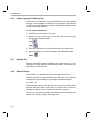
2.2.1
Opening More Than One Dis-Assembly Window
Multiple Dis-Assembly windows can be opened by selecting the command
View->Dis-Assembly or by using the Dis-Assembly Window button on the
Debug toolbar:
Dis-Assembly Window:
The first window tracks the location of the PC. When more than one
Dis-Assembly window appears, the title bar displays Dis-Assembly <n>,
where n is a unique window number.
2.2.2
Changing the Start Address
You can change the start address of the Dis-Assembly window by
double-clicking on the address field of the window. This brings up the View
Address dialog box that allows you to enter the start address you wish to use.
You may enter any absolute number or C expression that uses valid program
symbols.
The Basics of Code Composer Studio
2-3
Using the Dis-Assembly Window
2.2.3
Managing Breakpoints, Probe Points, and Profile Points from the
Dis-Assembly Window
To set or clear breakpoints, Probe Points, and profile points, place the cursor
on the line of interest in the Dis-Assembly window and select an appropriate
command from the Debug or Profiler menus or click the appropriate button on
the Project toolbar. Breakpoints may be quickly set by double-clicking on the
line of interest. These set points are indicated by a colored background on the
line. The color depends on what type of point is set. For example, if a
breakpoint and a Probe Point are set on the same line, a purple and blue
background appears on that line.
2.2.4
Changing Color Highlights
You can change the default display colors for the current PC and debugging
points (breakpoints/profile points/Probe Points) by selecting Option->Colors.
2.2.5
Setting Dis-Assembly Style Options
Code Composer Studio offers several options for changing the way you view
information in the Dis-Assembly window. The Dis-Assembly Style Options
dialog box allows you to input specific viewing options for your debugging
session. For instance, you may select hex or decimal as the addressing radix.
2-4
Using the Dis-Assembly Window
To Set Dis-Assembly Style Options
1) Select the command Option->Dis-Assembly Style.
OR
Right-click in the Dis-Assembly window. From the context menu, select
Properties->Dis-Assembly.
2) Enter your choices in the Dis-Assembly Style Options dialog box.
3) Click OK.
The contents of the Dis-Assembly window are immediately updated with the
new style.
2.2.6
Viewing Mixed C Source and Assembly Code
In addition to viewing disassembled instructions in the Dis-Assembly window,
the Code Composer Studio debugger enables you to view your C source
code interleaved with disassembled code.
To View Mixed C Source and Assembly Code
After loading a program onto your target or simulator:
1) Select View->Mixed Source/ASM. A check mark identifies when this
option is selected.
2) Select Debug->Go Main.
The debugger starts executing the program and stops execution at
main(). The associated C source file is automatically displayed in an Edit
window. (See Section 2.8, Resetting Your Target Processor for further
information.) Notice that the disassembled instructions for each C
statement appear within the source code. Just as in the Dis-Assembly
window, the location of the PC is highlighted in yellow.
You can choose to view the C source file with or without assembly code. To
change your selection, toggle View->Mixed Source/ASM or right-click in the
Edit window to open the context menu and select Mixed Mode or Source
Mode, depending on your current selection.
The Basics of Code Composer Studio
2-5
Using the Memory Window
2.3
Using the Memory Window
The Code Composer Studio debugger allows you to view the contents of
memory at a specific location.
To View the Contents of Memory
1) Select View->Memory.
OR
Click the View Memory button on the Debug toolbar.
Memory Window:
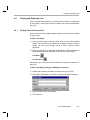
2) Before the Memory window is displayed, the Memory Window Options
dialog box appears. This dialog allows you to specify various
characteristics of the Memory window.
Enter the desired characteristics in the Memory Window Options dialog
box (see Section 2.3.1, Setting Memory Window Options).
3) Click OK. The Memory window appears.
To modify any of the characteristics of the active Memory window, right-click
in the Memory window and select Properties from the context menu. The
Memory Window Options dialog box appears.
To edit the contents of a memory location, double-click the appropriate
address in the Memory window or select Edit->Memory->Edit. The Edit
Memory dialog box appears (see Section 2.3.2, Editing a Memory Location).
2-6
Using the Memory Window
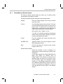
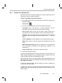
2.3.1
Setting Memory Window Options
The Memory Window Options dialog box allows you to specify various
characteristics of the Memory window.
The Memory Window Options dialog offers the following options:
Address
Enter the starting address of the memory location
you want to view.
Q Value
You can display integers using a Q value. This value
is used to represent integer values as more precise
binary values. A decimal point is inserted in the
binary value; its offset from the least significant bit
(LSB) is determined by the Q value as follows:
New_integer_value = integer / 2Q value
A Q value of xx indicates a signed 2s complement
integer whose decimal point is displaced xx places
from the least significant bit (LSB).
Format
From the drop-down list, select the format of the
memory display.
Use IEEE Float
Select this option if you want the display to use the
IEEE floating-point format.
Page
From the drop-down list, select the type of page:
Program, Data, or I/O.
Enable Reference Buffer
Select this checkbox to save a snapshot of a
specified area of memory that can be used for later
comparison.
For example, suppose you select Enable Reference
Buffer and specify an address range of
0x0000..0x002F. The contents of memory for the
specified range are saved in host memory. Every
time you halt the target, hit a breakpoint, refresh
memory, etc., the debugger compares the contents
of the Reference Buffer with the current contents of
memory. Any changes are displayed in red as you
scroll through this memory space in the Memory
window.
The Basics of Code Composer Studio
2-7
Using the Memory Window
Start Address
Enter the starting address of the memory locations
you want to save in the Reference Buffer. This field
only becomes active when Enable Reference Buffer
is selected.
End Address
Enter the ending address of the memory locations
you want to save in the Reference Buffer. This field
only becomes active when Enable Reference Buffer
is selected.
Update Reference Buffer Automatically
Select this checkbox to automatically overwrite the
contents of the Reference Buffer with the current
contents of memory at the specified range of
addresses. If this checkbox is not selected, the
contents of the Reference Buffer are not changed.
This option only becomes active when Enable
Reference Buffer is selected.
All input fields are C expression input fields. An expression containing a
symbol name can be used to specify the starting address in the Memory
Window Options dialog. For further information, see Section 2.3.3.1, Using
Symbols within Expressions.
Display Formats
The Memory window can display the contents of memory in many different
formats. The supported display formats are listed below:
2-8
C-style hex
Words are displayed with the prefix 0x
Hex
TI format for displaying hex numbers
Signed integer
Values are shown as signed integers
Unsigned integer
Values are shown as unsigned integers
Character
Character equivalent of the LSB of each word is
displayed
Packed character
Each word is shown as the sum of 8-bit characters
Floating point
Values are shown in decimal floating-point format
Exponential float
Values are shown in exponential floating-point
format
Binary
Values are shown in binary format
Using the Memory Window
2.3.2
Editing a Memory Location
You can edit a memory location in one of the following ways:
❏
❏
In the Memory window, double-click on the data you wish to edit, or
Select the Edit->Memory->Edit command.
Both of these methods open the Edit Memory dialog box. If you have
double-clicked on a memory location in the Memory window, the Address and
Data fields contain the address and data value of the selected location.
If you used the menu command, the Address and Data fields contain default
values. To get the desired address location, enter the address you wish to edit
in the Address field. Press Tab or click on the Data field and the content is
updated with the value at the specified address. To change the data value of
that location, enter the desired value into the Data field and click Done. You
can also use the scroll buttons on the Address field to move through the
memory locations.
If you double-click on a location in the Memory window, the default format of
the Data field is the same as in the Memory window.You can enter values in
either hex format (with prefix 0x) or in decimal format (with no prefix) if the
display format is integer. You can also enter floating-point values, provided
the display format is compatible.
All the input fields are C expression input fields.
2.3.3
C Expression Input Fields
All input fields that require a numerical value are C expression input fields. In
these input fields, you can enter any valid C expression, including the names
of C functions or assembly language labels. The expression is then reduced
to a single numerical value and displayed, as shown in the following
examples:
MyFunction
0x1000 + 2 * 35
(int) MyFunction + 0x100
PC + 0x10
The default display format for these fields is hexadecimal but can be changed
by using special formatting symbols, similar to the Watch window symbols
(see Section 8.3, Watch Window Display Formats).
The Basics of Code Composer Studio
2-9
Using the Memory Window
2.3.3.1
Using Symbols within Expressions
An expression containing a symbol name can be used for all fields requiring
numerical input. However, Code Composer Studio interprets symbols
differently depending on whether or not the object file contains symbolic
debugging information.
If a symbol is defined in a C source file and symbolic debugging information
(-g) is specified when building the file, the symbol is treated as a variable
representing the contents of memory at the specified address.
Without symbolic debugging information, all symbols are treated as
addresses.
For example, when using a symbol name to specify the starting address in
the Memory Window Options dialog or the Graph Property dialog box:
If symbolic debugging information is available, and you want to use the
address of a simple variable, you should prepend the symbol name (variable)
with an ampersand (&), the standard C-language notation for expressing an
address. Otherwise (without the ampersand), the expression evaluates to the
contents of the symbol. The exception is variables representing arrays; in
C-notation, specifying the name with the ampersand implies that you are
referring to the address at the start of the array.
If no symbolic debugging information is available, specify only the symbol
name (address).
2-10
CPU Registers
2.4
CPU Registers
The CPU and peripheral registers of the target processor can be viewed
using the Register window. The contents of registers can be edited using the
Edit Registers dialog.
2.4.1
Viewing Registers
To view the contents of the CPU registers of the target processor, select the
command View->CPU Registers->CPU Register. You can also display the
CPU Register window by selecting the View Registers button on the Debug
toolbar.
Register Window:
From the Register window, you can edit registers via the Edit Registers
dialog.
2.4.2
Editing Registers
To Edit the Contents of a Register
Select Edit->Edit Register. The Edit Registers dialog box appears.
OR
From the Register window, double-click a register or right-click in the window
and select Edit Register from the context menu.
The Edit Registers dialog offers the following options:
Register
Specify the register you want to edit by typing its name or by
selecting a register from the drop-down list.
Value
This field contains the current value of the specified register
displayed in hex. You can enter another value in this field in
hex (with the prefix 0x) or in decimal (with no prefix). You can
also enter any valid C expression.
After modifying the value of a register, click Close to apply your changes.
Click Close again to close the dialog box.
Note: Simulator - Peripheral Registers Not Supported
The simulator does not include peripheral register support.
The Basics of Code Composer Studio
2-11
Loading a COFF File
2.5
Loading a COFF File
To load a valid COFF file onto your actual/simulated target board, select
File->Load Program. In the Load Program dialog box, select the desired file
and click Open.
This command loads the data as well as the symbol information from the
COFF file.
2.5.1
Loading Symbol Information Only
To load symbol information only, select File->Load Symbol. In the Load
Symbol Info dialog box, select the desired file and click Open.
This functionality is useful in a debugging environment where the debugger
cannot or need not load the object code, such as when the code is in ROM.
This command clears the existing symbol table before loading the new one
but does not modify memory or set the program entry point.
2.5.2
Reloading a COFF File
To reload a valid COFF file onto your actual/simulated target board, select
File->Reload Program. Before reloading the program, a check is performed
to see if the file has been changed since the last load. If the file has changed,
both the program and its symbol information are reloaded. If no change is
detected, only the program is reloaded; its associated symbol table is not
reloaded.
This command is useful for reloading a program when target memory has
been corrupted.
2-12
Loading a COFF File
2.5.3
Setting Program Load Options
To open the Program Load Options dialog box, select Options->Program
Load. The Program Load Options dialog box offers the following options:
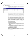
Perform verification after Program Load. By default, this checkbox is
checked. This means that Code Composer Studio will verify (by reading back
selected memory) that the program was loaded correctly. If you remove the
check from this option, Code Composer Studio will not perform this
verification.
Load Program After Build. If you check the Load Program After Build option,
the executable is loaded immediately upon building the project. This ensures
that the target contains the most up-to-date symbolic information generated
after a build.
The Basics of Code Composer Studio
2-13
Single Stepping
2.6
Single Stepping
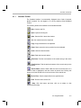
Use the following buttons from the Debug toolbar to single step through code.
Step Into: You can single step through the code by either clicking the
button on the Debug toolbar or by selecting Debug->StepInto. If you are in C
source mode, this command steps through a single C instruction; otherwise,
it steps through a single assembly instruction.
Step Over: You can use the step over command to step through and
execute individual statements in the current function. If a function call is
encountered, the function executes to completion unless a breakpoint is
encountered before it stops after the function call. You can step over code by
either clicking the button on the Debug toolbar or by selecting
Debug->StepOver.
You may view the file entirely in C or display the assembly files at the same
time. In C source mode (see Section 2.2.6, Viewing Mixed C Source and
Assembly Code), this command steps over an entire C instruction; otherwise,
it steps over a single assembly instruction. However, to protect the
processor's pipeline, several instructions following a delayed branch or call
may be considered part of the same statement. In this case, the step over
command may execute more than one instruction at a time.
Step Out: If you are inside a subroutine, you can select the step out
command to complete execution of the subroutine. The execution stops after
the current function returns to the calling function. You can step out by either
clicking the button on the Debug toolbar or by selecting Debug->StepOut.
In C source mode, the calling function is determined from the standard
runtime C stack using the local frame pointer; otherwise, the return address
to the calling function is assumed to be the value on the top of the stack. If
your assembly routine uses the stack to store other information, the step out
command does not function properly.
Run to Cursor: You can use the run to cursor feature to run the loaded
program until it encounters the Dis-Assembly window cursor position. You
can run to cursor by selecting Debug->Run to Cursor.
2-14
Single Stepping
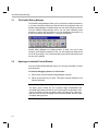
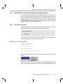
2.6.1
Multiple Stepping Operations
To Invoke a Stepping Command Multiple Times
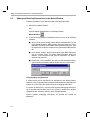
1) Select the command Debug->Multiple Operations.
2) In the Multiple Operations dialog box, select a stepping command from
the drop-down list.
3) Specify the number of times the command is to be invoked.
4) Click OK.
Repeat this procedure to invoke the same or another stepping command
multiple times.
The Basics of Code Composer Studio
2-15
Run, Halt, Animate, Run Free
2.7
Run, Halt, Animate, Run Free
Run: You can execute your program from the current PC location by
clicking the button on the Debug toolbar or by selecting Debug->Run.
Execution continues until a breakpoint is encountered.
Halt: You can stop execution of your program by clicking the button on
the Debug toolbar or by selecting Debug->Halt.
Animate: You can animate your program by clicking the button on the
Debug toolbar or by selecting Debug->Animate. The program runs until it
encounters a breakpoint. It updates the windows that are not connected to
any Probe Points and resumes execution. To halt animation, select
Debug->Halt. You can control the speed of animation by selecting
Option->Animate Speed.
Run Free: This command disables all breakpoints, including Probe Points
and profile points, before executing your program starting from the current PC
location. Select the command Debug->Run Free. Any operation that
accesses the target processor while in free run restores breakpoints. Use the
Debug->Halt command to stop execution. If you are emulating using a
JTAG-based device driver, this command also disconnects from the target
processor so you can remove the JTAG or MPSD cable. You can also perform
a hardware reset of your target processor while in free run.
Note: Simulator - Run Free Not Supported
When running the simulator, the run free capability is not available.
2-16
Run, Halt, Animate, Run Free
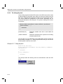
2.7.1
Setting Animation Speed
The animation speed is the minimum time between breakpoints. In animation
mode, the program executes until a breakpoint is encountered. At this
breakpoint, execution stops and all windows not connected to any Probe
Points are updated. The program execution resumes until the next
breakpoint. This animates the processor state at each breakpoint. A Probe
Point always resumes execution after updating the window connected to it.
To Set Animation Speed
1) Select the command Option->Animate Speed.
2) In the Animate Speed Properties dialog box, enter the animation speed
in seconds.
3) Click OK.
Program execution does not resume until the minimum time has expired since
the previous breakpoint.
To animate, select Debug->Animate. To halt animation, select Debug->Halt.
The Basics of Code Composer Studio
2-17
Resetting Your Target Processor
2.8
Resetting Your Target Processor
The following commands are available to reset your target processor:
Reset DSP: The Debug->Reset DSP command initializes all register
contents to their power-up state and halts the execution of your program. If
the target board does not respond to this command and you are using a
kernel-based device driver, the DSP kernel may be corrupt. In this case, you
must reload the kernel. The simulator initializes all register contents to their
power-up state, according to target simulation specifications.
Load Kernel: If you are using a kernel-based debugger (not JTAG), then the
DSP kernel is responsible for the communication to the host computer. If it is
corrupt, the device driver may not be able to communicate with the target. In
this case, you must execute the Debug->Load Kernel command to restore the
kernel to its proper state.
Restart: The Debug->Restart command restores the PC to the entry point for
the currently loaded program. This command does not start program
execution.
Go Main: The Debug->Go Main command sets a temporary breakpoint at the
symbol main in your program, and starts execution. The breakpoint is
removed when execution is halted or a breakpoint is encountered. This
provides a convenient way for C programmers to start their application. When
execution stops at main(), the associated source file is automatically loaded.
2.9
Copying Data Values
To Copy a Block of Memory to a New Location
1) Select Edit->Memory->Copy.
2) In the Setup for Copying dialog box, enter the Source information:
Address. The starting address of the block of memory to be copied.
Length. The length of the block of memory to be copied.
3) Enter the Destination information:
Address. The address to which the block of memory will be copied.
4) Click OK to perform the copy.
All the input fields are C expression input fields.
2-18
Filling Memory Locations
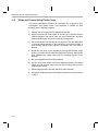
2.10
Filling Memory Locations
To Fill a Block of Memory with a Specified Value
1) Select Edit->Memory->Fill.
2) In the Setup Filling Memory dialog box, enter the following information:
Address. The start address of the block of memory to be filled.
Length. The length of the block of memory to be filled.
Fill Pattern. The pattern to use in filling the block of memory.
3) Click OK to perform the fill.
All locations starting from the start address to start address + length - 1 are
filled with the fill pattern entered in the Fill Pattern field.
All the input fields are C expression input fields.
2.11
Editing Variables
To Edit a Variable
1) Select Edit->Edit Variable.
2) In the Edit Variable dialog box, enter the following information:
Variable. The name of the variable to be edited.
Value. The new value.
3) Click OK to perform the edit.
The Edit Variable dialog box is also used when editing expressions in the
Watch window (see Section 8.2, Editing Variables in the Watch Window).
All the input fields are C expression input fields.
For TI fixed-point processors, if your actual/simulated target consists of
multiple pages, you can specify the specific page with the @ symbol. After
you type the symbol, enter one of the keywords: prog, data, or io. The
keyword specifies whether the page is a program, data or I/O page, as shown
in the following examples:
*0x1000@prog = 0
*0x1000@data = myVar
*0x2000@io = 0
The Basics of Code Composer Studio
2-19
Editing the Command Line
2.12
Editing the Command Line
The Command Line dialog provides a convenient way of entering expressions
or executing GEL functions You can execute any of the built-in GEL functions
or you can execute your own GEL functions that have been loaded (see
Section 12.5, Loading/Unloading GEL Functions).
To Execute Commands
1) Select Edit->Edit Command.
2) In the Command Line dialog box, enter an expression or GEL function in
the Command field.
3) Click OK to execute the command.
You can also enter and execute built-in GEL expressions or user-defined GEL
functions via the GEL toolbar. To access this toolbar, select View->GEL
Toolbar. The scrollable list in the GEL toolbar contains a history of the most
recently executed GEL functions. To execute a previously used command,
select the command and click the button.
Execute:
The following examples display commands that can be entered in the GEL
toolbar or the Command Line dialog:
Modify variables by entering expressions:
PC = c_int00
Load programs with built-in GEL functions:
GEL_Load("c:\\myprog.out")
Run your own GEL functions:
MyFunc()
2-20
Refreshing Windows
2.13
Refreshing Windows
All windows usually show the current status of the target board. However, if
you connect a window to a Probe Point, the window may not contain the latest
information (see Chapter 4, Breakpoints and Probe Points). To update a
window, select Window->Refresh. This command updates the active window
with the current target data.
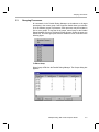
2.14
Viewing the Call Stack
You can use the Call Stack window to examine the series of function calls that
led to the current location in the program that you are debugging. To display
the call stack, select View->Call Stack or click the View Stack button on the
Debug toolbar.
View Stack:
To display the source code for a calling function in a list, double-click on the
desired function. An Edit window containing the source code appears with the
cursor set to the current line within the desired function. When you select a
function in the Call Stack window, you can also observe local variables that
are within the scope of the function.
The call stack only works with C programs. Calling functions are determined
by walking through the linked list of frame pointers on the runtime stack. Your
program must have a stack section and a main function; otherwise, the call
stack displays the message: C source is not available.
2.14.1
Observing Local Variables
You can observe local variables (automatic variables) of a function that is not
currently running but resides in the call stack. Use the Call Stack window to
change the scope to that of the function you are interested in. You can then
observe (or add to the Watch window) all local variables of that function.
The Basics of Code Composer Studio
2-21
Saving and Restoring Your Workspace
2.15
Saving and Restoring Your Workspace
You can save and restore your current working environment, called a
workspace, between debugging sessions. You can also switch between
different working environments in the same debugging session.
To Save a Workspace
1) Select File->Workspace->Save Workspace.
2) In the Save As dialog box, enter a name for the workspace in the File
name field.
3) Click Save.
When you exit Code Composer Studio, your current workspace is
automatically saved in a file named default.wks (see Section 2.15.2, The
Default Workspace).
To Load a Workspace
1) Select File->Workspace->Load Workspace.
2) In the Load Workspace dialog box, enter the name of the workspace file
in the File name field.
3) Click Open.
You can automatically load a particular workspace every time you start Code
Composer Studio (see Section 2.15.1, Automatically Loading Your
Workspace).
Things that are Saved in the Workspace
❏
❏
❏
❏
❏
❏
❏
❏
❏
2-22
Parent windows (including size and position)
Child windows (including size and position)
Breakpoints, Probe Points, profile points
Profiler options
Current project
Currently loaded GEL functions
Memory map
Animation speed option
File I/O setup
Saving and Restoring Your Workspace
Things that are Not Saved in the Workspace
❏
❏
❏
❏
❏
❏
❏
❏
Current font
Current color scheme
Target memory, program, or processor state
Edit and find/replace floating tools
Error and progress messages in the build window
GEL output windows
Scan dependency window
Disassembly style options
Note: Font and Color Scheme Saved
Your font and color scheme, along with profiler options, memory map, and
animate speed, are automatically saved and restored between sessions in a
file named cc_user.dat.
Note: Initializing Target Processor
You can initialize your target processor state using the GEL extension
language (see Section 3.6, Auto-Executing GEL Functions).
The Basics of Code Composer Studio
2-23
Saving and Restoring Your Workspace
2.15.1
Automatically Loading Your Workspace
You can automatically load a particular workspace every time you start Code
Composer Studio. To do this, you must name the workspace as the first
command line parameter when starting the application. This parameter must
end in .wks, for Code Composer Studio to recognize it as a workspace file.
Otherwise, Code Composer Studio will attempt to load it as a GEL file.
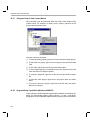
To Autoload a Workspace (Windows 95/98/NT)
1) In Windows Explorer, select the Code Composer Studio executable.
2) Right-click on the executable and select Create Shortcut to create a
shortcut to the executable.
3) Right-click on the shortcut that is created and select Properties.
4) In the Properties dialog box, select the Shortcut tab.
5) Verify that the Target field contains the path name and file name of the
Code Composer Studio executable. For example: c:\ti\cc\bin\cc_app.exe.
6) At the end of this path name, add the name of your workspace file (which
must end in .wks). For example: c:\ti\cc\bin\cc_app.exe myspace.wks.
Note: Default Workspace
If you specify the file default.wks, the default workspace will be
automatically loaded every time you start Code Composer Studio.
2.15.2
The Default Workspace
Your current workspace is automatically saved in a file named default.wks
when you exit Code Composer Studio. If you wish to resume where you left
off, start Code Composer Studio and load default.wks with the
File->Workspace->Load Workspace command. If you start Code Composer
Studio with default.wks as the first program parameter on the command line,
the default workspace is automatically loaded every time you start Code
Composer Studio.
You can setup Code Composer Studio to automatically load the default
workspace every time you start the application. This provides a way to
automatically save and restore your environment between sessions.
2-24
Saving and Restoring Your Workspace
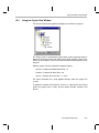
To Autoload a Workspace and GEL Files On Start Up
You can load both your workspace and the associated GEL files when you
start Code Composer Studio:
1) With Code Composer Studio running, load the desired GEL functions and
save the entire environment as a workspace by selecting
File->Workspace->Save Workspace. (See Section 12.5, Loading/
Unloading GEL Functions).
2) Setup Code Composer Studio to automatically load this workspace on
startup (see Section 2.15.1, Automatically Loading Your Workspace).
If you are operating in a multiprocessor environment, see Section 3.6,
Auto-Executing GEL Functions.
The Basics of Code Composer Studio
2-25
Chapter 3
Multiprocessing With Code Composer Studio
Code Composer Studio can support concurrent debugging sessions of
multiple processors. The Parallel Debug Manager is used to broadcast
commands to all processors and to select them individually. Before you can
use the Parallel Debug Manager, you must configure the multiprocessing
environment using the Code Composer Setup program. Once this
configuration is set up and Code Composer Studio is invoked, the Parallel
Debug Manager menu bar appears on your screen.
Note: Simulator - Multiprocessing Not Supported
The simulator does not support multiple DSP systems. You must use the
emulator version of the Code Composer Studio debugger along with a
multi-DSP target board.
Topic
Page
3.1
The Parallel Debug Manager. . . . . . . . . . . . . . . . . . . . . . . . . . . . . . . . 3–2
3.2
Opening an Individual Parent Window . . . . . . . . . . . . . . . . . . . . . . . 3–2
3.3
Grouping Processors . . . . . . . . . . . . . . . . . . . . . . . . . . . . . . . . . . . . . 3–3
3.4
Multiprocessor Broadcast Commands . . . . . . . . . . . . . . . . . . . . . . . 3–5
3.5
Broadcasting GEL Commands. . . . . . . . . . . . . . . . . . . . . . . . . . . . . . 3–6
3.6
Auto-Executing GEL Functions . . . . . . . . . . . . . . . . . . . . . . . . . . . . . 3–7
3.7
Global Breakpoints . . . . . . . . . . . . . . . . . . . . . . . . . . . . . . . . . . . . . . . 3–9
3-1
The Parallel Debug Manager
3.1
The Parallel Debug Manager
The Parallel Debug Manager allows you to synchronize multiple processors.
If you have several processors and a device driver that supports them, the
Parallel Debug Manager is enabled when you start Code Composer Studio.
From the Parallel Debug Manager menu, you can open individual parent
windows to control each processor or you can broadcast commands to a
group of processors (see Section 3.3, Grouping Processors).
Parallel Debug Manager is a floating toolbar. To keep it on top of other
windows, select Options->Always On Top. You can change the shape of the
menu bar by resizing it. The command buttons and menus wrap around to fit
the size of the window.
3.2
Opening an Individual Parent Window
From the Parallel Debug Manager menu, you can open a window to control
each processor.
To Select A Debugging Session on a Processor
1) Select Open from the Parallel Debug Manager menu bar.
2) Select the processor by its name. This opens a parent window for the
selected processor.
Note: Current System Configuration
The Open menu contains the list of physical target boards/DSPs and
simulated DSPs that are defined in your current system configuration. If the
correct processor list does not appear under the Open menu, make sure
that you have correctly configured Code Composer Studio with the Code
Composer Setup program.
3-2
Grouping Processors
3.3
Grouping Processors
All commands in the Parallel Debug Manager are broadcast to all target
processors in the current group. Code Composer Studio allows you to define
up to 32 different groups of processors. Each processor may be included in
one or more groups. To view the list of groups, select Group on the Parallel
Debug Manager menu bar. This lists all groups by name. Select the group you
wish to use. The active group has a check beside the name, as shown in the
following figure:
To Edit a Group
Select Group->Edit from the Parallel Debug Manager. The Groups dialog box
appears.
Multiprocessing With Code Composer Studio
3-3
Grouping Processors
The Groups dialog box displays group names in the first column and
processor names across the top. Each entry in the table is either Y (yes) or N
(no). When these entries are Y, the processor for that column is included in
the group in the same row. Only processors that are included in the current
group receive broadcast messages.
Group names can be edited directly and must be unique. By default, a group
named FirstBoard is created that includes all processors. This group can be
modified, but you cannot delete it. This ensures that there is always at least
one group available.
To Create a New Group
In the Groups dialog box, click New. Code Composer Studio generates a new
group with a unique name. Initially, none of the processors are included in the
new group.
To Include a Processor in a Group
1) Find the column corresponding to the processor you wish to include.
2) Find the row corresponding to the group where you want to include the
processor.
3) Click the cell where the column and row intersect. When a Y appears, the
processor is included in the group.
To Delete a Group
1) Using the mouse or the arrow keys, highlight the group name.
2) Choose Remove.
3-4
Multiprocessor Broadcast Commands
3.4
Multiprocessor Broadcast Commands
All commands in the Parallel Debug Manager are broadcast to all target
processors in the current group (see Section 3.3, Grouping Processors). If
the DSP device driver supports synchronous operation, each of the following
commands is synchronized to start at the same time on each processor.
Locked Step
You can use locked step to single step all processors that are not already
running.
Locked Step-Over
You can use locked step-over command to execute step-over on all
processors that are not already running.
Locked Step-Out
If all the processors are inside a subroutine, you can use locked step-out to
execute the Step-Out command on all the processors that are not already
running.
Synchronous Run
This command sends a global Run command to all processors that are not
already running.
Synchronous Halt
This command halts all processors simultaneously.
Synchronous Animation
This command starts animating all the processors that are not already
running. See Section 2.7, Run, Halt, Animate, Run Free for details.
Multiprocessing With Code Composer Studio
3-5
Broadcasting GEL Commands
3.5
Broadcasting GEL Commands
To broadcast GEL commands
1) Select Group->Broadcast Command from the Parallel Debug Manager
menu. This opens the Broadcast Command dialog box.
2) Enter a built-in GEL function or user-defined GEL function in the
command box (see Section 12.5, Loading/Unloading GEL Functions).
3) Click OK or press Enter to broadcast the command to each processor in
the current group.
Note: Broadcast GEL Commands
Broadcast GEL commands are restricted to processors whose parent
window is also open.
3-6
Auto-Executing GEL Functions
3.6
Auto-Executing GEL Functions
GEL functions allow you to configure the development environment according
to your needs. For example, you can configure a control window for a specific
CPU to initialize the wait states for the memory system each time the window
opens. Or you can set up a number of tasks you want performed each time
you open the control window.
Instead of loading your GEL file using the File->Load GEL command each
time and then executing the GEL function, you can use the Open->CPU
command to pass a GEL file name to each control window each time you
open it. This informs the control window to scan in and load the specified GEL
file. You may execute the function as well. Do this by naming one of your GEL
functions in the specified file StartUp(). When a GEL file is loaded into Code
Composer Studio, the file is searched for a function defined as StartUp(). If
the function is found, it is automatically executed.
To Autoload and Execute a GEL File When You Open a Control Window
1) In the Parallel Debug Manager menu, select Options->Startup to open
the StartUp Files dialog box. This dialog box lists all the CPUs and
provides a field where you can specify the GEL file for each CPU.
2) In this field, add the name of the GEL file that contains your GEL
functions. For example, cpu_a myfile.gel.
Now each time you open the control window for cpu_a, the GEL file myfile.gel
is automatically scanned and loaded into Code Composer Studio. If you have
a GEL function defined as StartUp(), it is also executed.
If you have a common file that all your CPUs load on startup, you can place
this filename in the command line of the Properties dialog box of the Code
Composer Studio icon.
Multiprocessing With Code Composer Studio
3-7
Auto-Executing GEL Functions
To Autoload a Workspace and Associated GEL Files On Start Up
Code Composer Studio allows you to load both your workspace and the
associated GEL files immediately on start up, as follows:
1) In the Parallel Debug Manager menu, select Options->Startup.
2) In the StartUp Files dialog box, enter the GEL file names corresponding
to each CPU and click OK.
3) Save the setup as a workspace by selecting File->Save Workspace.
4) In the Save As dialog box, enter the name of the workspace (with the .wks
extension) in the File name field (see Section 2.15.1, Automatically
Loading Your Workspace).
5) Click Save.
3-8
Global Breakpoints
3.7
Global Breakpoints
Global breakpoints allow breakpoints on a given processor to halt other
processors in a multiprocessor environment. JTAG-based device drivers use
the EMU0/1 pins that trigger other processors to stop at the same time. When
this option is enabled, all processors in the current group halt if any processor
included in the current group encounters a breakpoint.
To enable global breakpoints on all processors in the current group, select
Options->Global Breakpoints from the Parallel Debug Manager menu bar. A
check mark beside this menu item indicates that global breakpoints are
enabled. By changing the current group (see Section 3.3, Grouping
Processors), you can control which processors are triggered by global
breakpoints.
Multiprocessing With Code Composer Studio
3-9
Chapter 4
Breakpoints and Probe Points
This chapter describes how you can set breakpoints to control the execution
of your program and how to set Probe Points for signal analysis.
Topic
Page
4.1
Breakpoints . . . . . . . . . . . . . . . . . . . . . . . . . . . . . . . . . . . . . . . . . . . . . 4–2
4.2
Conditional Breakpoints . . . . . . . . . . . . . . . . . . . . . . . . . . . . . . . . . . . 4–6
4.3
Hardware Breakpoints. . . . . . . . . . . . . . . . . . . . . . . . . . . . . . . . . . . . . 4–7
4.4
Probe Points . . . . . . . . . . . . . . . . . . . . . . . . . . . . . . . . . . . . . . . . . . . . 4–8
4.5
Conditional Probe Points . . . . . . . . . . . . . . . . . . . . . . . . . . . . . . . . . 4–12
4.6
Hardware Probe Points . . . . . . . . . . . . . . . . . . . . . . . . . . . . . . . . . . . 4–13
4-1
Breakpoints
4.1
Breakpoints
Breakpoints stop the execution of the program. When the program is stopped,
you can examine the state of your program, examine or modify variables,
examine the call stack, etc. You can set a breakpoint, by using the Toggle
Breakpoint button on the Project toolbar or by selecting Debug->Breakpoints.
The latter brings up the Break/Probe/Profile Points dialog box. When a
breakpoint is set, you can enable or disable it.
4.1.1
Designer Notes (Kernel-Based Code Composer Studio Debugger)
Follow these guidelines to avoid possible corruption of the processor pipeline:
4.1.2
❏
Do not set a breakpoint on any instructions executed as part of a delayed
branch or call.
❏
Do not set a breakpoint on the last one or two instructions before the end
of a block repeat instruction.
Adding and Deleting Breakpoints
To Add a Breakpoint Using the Breakpoint Dialog Box
1) Select Debug->Breakpoints. The Break/Probe/Profile Points dialog box
appears with the Breakpoints tab selected.
2) In the Breakpoint Type field, select either Break at Location
(unconditional) or Break at Location if Expression is TRUE (conditional).
3) Enter the location where you want to set the breakpoint, using either of
the following formats:
■
For an absolute address, enter any valid C expression, the name of
a C function, or a symbol name.
■
Enter a breakpoint location based on your C source file. This is
convenient when you do not know where the C instruction ends up in
the executable. The format for entering a location based on the C
source file is as follows: fileName line lineNumber
4) If you selected a conditional breakpoint in step 2, you must enter the
condition in the Expression field.
5) Click Add to create a new breakpoint. This causes a new breakpoint to
be created and enabled.
6) Click OK to close the dialog box.
4-2
Breakpoints
To Add a Breakpoint Using the Toolbar
Using the Toggle Breakpoint buftton on the Project toolbar is the easiest way
to set and clear breakpoints at any location in the program. The breakpoint
dialog box allows you to set more complex breakpoints, such as conditional
breakpoints or hardware breakpoints.
1) Put the cursor in the line where you want to set the breakpoint. You can
set a breakpoint in either a Dis-Assembly window or an Edit window
containing C source code.
2) Click the Toggle Breakpoint button on the Project toolbar. The line is
highlighted.
Toggle Breakpoint:
To Remove a Breakpoint Using the Toolbar
.
1) Put the cursor in the line containing the breakpoint.
2) Click the Toggle Breakpoint button on the Project toolbar.
To Change an Existing Breakpoint
1) Select Debug->Breakpoints. The Break/Probe/Profile Points dialog
box.appears with the Breakpoints tab selected.
2) Select a breakpoint in the Breakpoint window. The selected breakpoint is
highlighted and the Breakpoint Type, Location, and Expression fields are
updated to match the selected breakpoint.
3) Edit the breakpoint Type, Location, and/or Expression fields as required.
4) Click Replace to change the currently selected breakpoint.
5) Click OK to close the dialog box.
To Delete an Existing Breakpoint
1) Select Debug->Breakpoints. The Break/Probe/Profile Points dialog
box.appears with the Breakpoints tab selected.
2) Select a breakpoint in the Breakpoint window.
3) Click Delete to delete the breakpoint.
4) Click OK to close the dialog box.
Breakpoints and Probe Points
4-3
Breakpoints
To Delete All Breakpoints Using the Breakpoint Dialog Box
1) Select Debug->Breakpoints. The Break/Probe/Profile Points dialog box
appears with the Breakpoints tab selected.
2) Click Delete All.
3) Click OK to close the dialog box.
To Delete All Breakpoints Using the Toolbar
Click the Remove All Breakpoints button on the Project toolbar.
Remove All Breakpoints:
4.1.3
Enabling and Disabling Breakpoints
When a breakpoint is set, it can be disabled or enabled. Disabling a
breakpoint provides a quick way of suspending its operation while retaining
the location and type of the breakpoint.
To Enable a Breakpoint
1) Select Debug->Breakpoints. The Break/Probe/Profile Points dialog box
appears with the Breakpoints tab selected.
2) Select the breakpoint you wish to enable from the Breakpoint window.
The checkbox beside the breakpoint is empty to indicate that it is
currently disabled.
3) Click on the breakpoint checkbox. This adds a check to the box, indicating
that the breakpoint is now enabled.
4) Click OK to close the dialog box.
To Disable a Breakpoint
1) Select Debug->Breakpoints. The Break/Probe/Profile Points dialog box
appears with the Breakpoints tab selected.
2) Select the breakpoint you wish to disable from the list. The breakpoint
checkbox is checked to indicate that it is currently enabled.
3) Click on the breakpoint checkbox. This removes the check from the box,
indicating that the breakpoint is now disabled.
4) Click OK to close the dialog box.
4-4
Breakpoints
To Enable All Breakpoints
1) Select Debug->Breakpoints. The Break/Probe/Profile Points dialog box
appears with the Breakpoints tab selected.
2) Click Enable All. This button allows you to quickly enable all breakpoints
in the breakpoint list.
3) Click OK to close the dialog box.
To Disable All Breakpoints
1) Select Debug->Breakpoints. The Break/Probe/Profile Points dialog
box.appears with the Breakpoints tab selected.
2) Click Disable All. This button allows you to quickly disable all breakpoints
in the breakpoint list.
3) Click OK to close the dialog box.
Breakpoints and Probe Points
4-5
Conditional Breakpoints
4.2
Conditional Breakpoints
Every conditional breakpoint has its own conditional expression. When the
location of the conditional breakpoint is reached, the expression is evaluated.
If the result of the expression is false, the processor resumes execution
without updating the display; otherwise, the display is updated as if a
traditional breakpoint were hit.
You can also define GEL (General Extension Language) files to meet
conditions that must be satisfied for a breakpoint to be enabled.
To enter the GEL file name
1) Select Debug->Breakpoints. The Break/Probe/Profile Points dialog box
appears with the Breakpoints tab selected.
2) From the “Breakpoint type” drop-down list, select “Break at Location if
expression is TRUE”. Only when this selection is made will the
Expression field become active, allowing you to enter the GEL file name.
3) Enter your GEL file name in the Expression field. This ensures that the
breakpoint is only enabled if your condition is met.
For more information on GEL files and their implementation, see Chapter 12,
The General Extension Language (GEL),
Note: Target Processor Halts
The target processor halts while the expression is evaluated by the host.
This means that the target application may not be able to meet real-time
constraints with conditional breakpoints set.
4-6
Hardware Breakpoints
4.3
Hardware Breakpoints
Hardware breakpoints differ from software breakpoints in that they do not
modify the target program. Hardware breakpoints are useful for setting
breakpoints in ROM memory or breaking on memory accesses instead of
instruction acquisitions. A breakpoint can be set for a particular memory read,
memory write, or memory read or write. Memory access breakpoints are not
shown in the Edit or Memory windows.
Note: Simulator - Hardware Breakpoints Not Supported
Hardware breakpoints cannot be implemented on a simulated DSP target.
Hardware breakpoints can also have a count, which determines the number
of times a location is encountered before a breakpoint is generated. If the
count is1, a breakpoint is generated every time.
To Add a Hardware Breakpoint
1) Select Debug->Breakpoints. The Break/Probe/Profile Points dialog
box.appears with the Breakpoints tab selected.
2) In the Breakpoint type field, choose H/W Break at location for instruction
acquisition breakpoints or choose Break on <bus> <Read|Write|R/W> at
location for a memory access breakpoint.
3) Enter the program or memory location where you want to set the
breakpoint. Use one of the following methods:
■
For an absolute address, you can enter any valid C expression, the
name of a C function, or a symbol name.
■
Enter a breakpoint location based on your C source file. This is
convenient when you do not know where the C instruction is in the
executable. The format for entering in a location based on the C
source file is as follows: fileName line lineNumber
4) Enter the number of times the location is hit before a breakpoint is
generated, in the Count field. Set the count to 1 if you wish to break every
time.
5) Click Add to create a new breakpoint. This causes a new breakpoint to
be created and enabled.
6) Click OK to close the dialog box.
Breakpoints and Probe Points
4-7
Probe Points
4.4
Probe Points
Probe Points allow you to cause an update of a particular window or to read
and write samples from a file that occur at a specific point in your algorithm.
This connects a signal probe to that point in your algorithm. When the Probe
Point is set, you can enable or disable them just like breakpoints.
When a window is created, by default, it is updated at every breakpoint.
However, you can change this so the window is updated only when the
program reaches the connected Probe Point. When the window is updated,
execution of the program is continued.
Along with Code Composer Studio's file I/O capabilities, you can use Probe
Points to connect streams of data to a particular point in the DSP code. When
the Probe Point is reached in the algorithm, data is streamed from a specific
memory area to file or from the file to memory. See Section 5.1, File Input/
Output for information.
Note: Target Processor Halts on Probe Point
The target processor is temporarily halted by the host processor when a
Probe Point is encountered. Therefore, the target application may not be
able to meet real-time constraints when using Probe Points.
4.4.1
Adding and Deleting Probe Points
To Add a Probe Point
You can create Probe Points by placing the cursor on the line in a source file
or Dis-Assembly window and clicking the Probe Point button on the Project
toolbar. Probe Points must be connected to a window or file (see Section
4.4.2, Connecting Probe Points). Selecting Debug->Probe Points allows you
to set more complex Probe Points, such as conditional or hardware Probe
Points.
Toggle Probe Point:
4-8
Probe Points
To Delete an Existing Probe Point
1) Select Debug->Probe Points. The Break/Probe/Profile Points dialog box
appears with the Probe Points tab selected.
2) Select a Probe Point in the Probe Point window.
3) Click Delete.
4) Click OK to close the dialog box.
To Delete All Probe Points Using the Probe Point Dialog Box
1) Select Debug->Probe Points. The Break/Probe/Profile Points dialog box
appears with the Probe Points tab selected.
2) Click Delete All.
3) Click OK to close the dialog box.
To Delete All Probe Points Using the Toolbar
Click the Remove All Probepoints button on the Project toolbar.
Remove All Probepoints:
4.4.2
Connecting Probe Points
To Connect a Display Window to a Probe Point
1) Open the window that you want to connect to.
2) Create the Probe Point by placing the cursor on the line where you want
the point set and clicking on the Toggle Probe Point button on the Project
toolbar.
Toggle Probe Point:
3) Select Debug->Probe Points. The Break/Probe/Profile Points dialog box
appears with the Probe Points tab selected. In the Probe Point window,
the new Probe Point that you have created appears. This Probe Point
indicates it currently has no connection.
Select this Probe Point to make it current. You can now edit its fields in
the dialog box.
4) Select a type of Probe Point from the Probe type drop-down list. The
default is unconditional. This means that every time the execution of the
code reaches the Probe Point, its connected file or window is updated
Breakpoints and Probe Points
4-9
Probe Points
and execution of the code continues after the update. You can change the
Probe Point to a conditional Probe Point to activate the probe only if the
expression is evaluated to be true.
5) Enter the location at which you want to set the Probe Point by using either
of the following methods. If you used the Toggle Probe Point button, this
field is already filled with the appropriate value.
■
For an absolute address, you can enter any valid C expression, the
name of a C function, or the name of an assembly language label.
■
Enter a Probe Point location based on your C source file. This is
convenient when you do not know where the C instruction is in the
executable. The format for entering in a location based on the C
source file is as follows: fileName line lineNumber
6) If you selected a conditional Probe Point in step 4, then you must enter
the condition in the Expression field.
7) Connect the window or file to the Probe Point. The Connect To drop-down
list contains all the files and windows that can be connected to the Probe
Point. From this list select the appropriate item.
8) Click Add to create the new Probe Point or click Replace to modify the
existing Probe Point.
4.4.3
Enabling and Disabling Probe Points
Once a Probe Point is set, it can be enabled or disabled. Disabling a Probe
Point provides a quick way of suspending its operation temporarily, while
retaining the location and type of the Probe Point.
Note: Windows Do Not Update
Windows connected to Probe Points that are disabled are not updated.
4-10
Probe Points
To Enable a Probe Point
1) Select Debug->Probe Points. The Break/Probe/Profile Points dialog box
appears with the Probe Points tab selected.
2) Select the Probe Point you wish to enable from the Probe Point window.
The Probe Point checkbox is empty when the Probe Point is disabled.
3) Click on the Probe Point checkbox. This puts a check in the box,
indicating that the Probe Point is now enabled.
4) Click OK to close the dialog box.
To Disable a Probe Point
1) Select Debug->Probe Points. The Break/Probe/Profile Points dialog box
appears with the Probe Points tab selected.
2) Select the Probe Point you wish to disable from the Probe Point window.
The Probe Point checkbox is checked when the Probe Point is enabled.
3) Click on the Probe Point checkbox. This removes the check from the box,
indicating that the Probe Point is now disabled.
4) Click OK to close the dialog box.
To Enable All Probe Points
1) Select Debug->Probe Points. The Break/Probe/Profile Points dialog box
appears with the Probe Points tab selected.
2) Click Enable All. All checkboxes now contain a check mark.
3) Click OK to close the dialog box.
To Disable All Probe Points
1) Select Debug->Probe Points. The Break/Probe/Profile Points dialog box
appears with the Probe Points tab selected.
2) Click Disable All. All checkboxes change to empty.
3) Click OK to close the dialog box.
Breakpoints and Probe Points
4-11
Conditional Probe Points
4.5
Conditional Probe Points
Every conditional Probe Point has its own conditional expression. When the
processor reaches the location of the conditional Probe Point, it evaluates the
expression. If the result of the expression is false, the processor resumes
execution as if it did not encounter a Probe Point. If the expression is true, it
performs as if a standard Probe Point were hit (see Section 4.4, Probe
Points).
You can also connect GEL (General Extension Language) files that you
define to meet conditions that must be satisfied for the particular Probe Point
to be enabled.
To enter the GEL file name
1) Select Debug->Probe Points. The Break/Probe/Profile Points dialog box
appears with the Probe Points tab selected.
2) From the “Probe type” drop-down list, select “Probe at Location if
expression is TRUE”. Only when this selection is made will the
Expression field become active, allowing you to enter the GEL file name.
3) Enter the GEL file name in the Expression field. This ensures that the
Probe Point is only enabled if your condition is met.
For more information on GEL files and their implementation, see Chapter 12,
The General Extension Language (GEL).
4-12
Hardware Probe Points
4.6
Hardware Probe Points
Hardware Probe Points operate the same as regular Probe Points, except
they are implemented using hardware breakpoints instead of software
breakpoints (see Section 4.3, Hardware Breakpoints). Hardware Probe
Points are useful for setting probes in ROM memory or tracing memory
accesses.
Note: Target Processor Halts on Probe Point
The target processor is temporarily halted by the host processor when it
encounters a hardware Probe Point. Therefore, the target application may
not be able to meet real-time constraints when using hardware Probe
Points.
Note: Simulator - Hardware Probe Points Not Supported
Hardware breakpoints (and thus Probe Points) cannot be implemented on
a simulated DSP target.
To Trace Memory Accesses
The following steps allow you to create a file object that stores the data at the
memory location you wish to trace (see Section 5.1, File Input/Output).
1) Select File->File I/O.
2) In the File I/O dialog box, click Add Probepoint. The Break/Probe/Profile
Points dialog box appears with the Probe Points tab selected.
3) In the Probe type field from the drop-down list, select probe on <bus>
<Read|Write|R/W> at location.
4) In the Location field, enter the memory location you want to trace.
5) Select the file object from the Connect To drop-down list.
6) Click Add to create and enable a new Probe Point.
7) Click OK to close the dialog box.
Breakpoints and Probe Points
4-13
Chapter 5
Using the File Input/Output Capabilities
This chapter describes how you can stream files into your actual or simulated
target as signals. It also tells you how to load and store PC files with target
memory values.
Topic
Page
5.1
File Input/Output . . . . . . . . . . . . . . . . . . . . . . . . . . . . . . . . . . . . . . . . . 5–2
5.2
Loading a Data File . . . . . . . . . . . . . . . . . . . . . . . . . . . . . . . . . . . . . . . 5–7
5.3
Storing a Data File . . . . . . . . . . . . . . . . . . . . . . . . . . . . . . . . . . . . . . . . 5–7
5-1
File Input/Output
5.1
File Input/Output
Code Composer Studio allows you to stream, or transfer, data to or from the
actual/simulated target from a PC file. This is a great way to simulate your
code using known sample values. The File I/O feature uses the Probe Point
concept, which allows you to extract/inject samples or take a snapshot of
memory locations at a point you define (Probe Point). A Probe Point can be
set at any point in your algorithm (similar to the way a breakpoint is set). When
the execution of the program reaches a Probe Point, the connected object
(whether it is a file, graph, or memory window) is updated. Once the
connected object is updated, execution continues. Using this concept, if we
set a Probe Point at a specific point in the code and then connect a file to it,
you can implement file I/O functionality.
You can associate a file with either an input or an output signal. At a specific
Probe Point, a stream of data can be either read from or written to a specified
file.
Note: Real-Time Data Transfer
File I/O does not support real-time data transfer. Select
Help->Tools->RTDX for information on using Real-Time Data Exchange
(RTDX).
To Stream Data To/From a File
1) Before you specify information on the file, set a Probe Point by placing
your cursor at the point where you want to set the Probe Point. Click the
Toggle Probe Point button on the Project toolbar. Leave the Probe Point
unconnected. The Probe Point tells the Code Composer Studio debugger
when you want to start streaming data from/to the file. That is, once the
execution of the code reaches this point, the Code Composer Studio
debugger updates (or reads from) the file that is connected to the Probe
Point. When it is finished, execution continues.
Toggle Probe Point:
2) Select File->File I/O. A File I/O dialog box appears. The File I/O dialog
prompts you for specific information. Choose either the File Input or the
File Output tab.
5-2
File Input/Output
3) Click Add File under either the File Input or the File Output tab. The File
Input dialog box appears.
❏
Navigate to the folder that contains the file you wish to use.
❏
Highlight the file name in the main window of the dialog; the name
appears in the File name field. The data file can be either a COFF
object file or a Code Composer Studio data file (see Section 5.1.2,
Data File Formats).
❏
Click Open. The file name appears in the File I/O dialog box. You can
repeat this procedure to select additional file for either File Input or
File Output.
4) When you insert a file in the File I/O dialog box, it is not connected to a
Probe Point. Notice that the Probepoint field shows the words “Not
Connected”.
To connect a file to a Probe Point, click Add Probepoint. The Break/
Probe/Profile Points dialog box appears with the Probe Points tab
selected.
❏
In the Probe Point list, highlight the Probe Point you want to connect
to. Notice that the Probe Point has “No Connection”.
❏
From the Connect To drop-down list, select the appropriate file.
❏
Click Replace. Notice that the Probe Point list now shows that the
Probe Point is connected to the file you have selected.
❏
Click OK. The Probepoint field in the File I/O dialog box show the
word “Connected” when a file has been successfully connected to a
Probe Point.
5) In the File I/O dialog box, enter values in the Address and Length fields
for each file selected.
The Address field specifies where you want the data transferred to (File
Input) or from (File Output). You can enter either a valid label or a numeric
address in this field.
The Length field indicates how many samples are to be transferred to
(File Input) or from (File Output) the target board every time the selected
Probe Point is reached.
You can enter affny valid C expression in the Address and Length fields.
These expressions are recalculated every time samples are read from or
written to the target. This means that if you enter a symbol in this field that
later changes in value, you do not have to reenter this parameter.
6) Click OK. The parameters you have entered will be verified.
Using the File Input/Output Capabilities
5-3
File Input/Output
Wrap Around Mode
Under the File Input tab, you can select the Wrap Around checkbox. You can
use wrap around mode to loop a file so that when the end of the file is
reached, access starts from the top. This feature is useful when you want to
generate a periodic signal from a file. If wrap around mode is not selected and
the end of file is reached, you are prompted with a message indicating the
end of file condition and the program is halted.
5-4
File Input/Output
5.1.1
File I/O Controls
When you enter data in the File I/O dialog box and click OK, control windows
appear that allow you to monitor and control the progress of the file I/O
activity.
The following are features of the control windows:
5.1.2
❏
Play button. Resumes file I/O transactions after a pause.
❏
Stop button. Halts all transfer of data from/to the file regardless of
whether a Probe Point was hit or not. This button can be used to
temporarily halt file I/O transfers.
❏
Rewind to Beginning button. Resets the file. For file input, the next
samples are read from the top of the file. For file output, all existing
samples are deleted and the new samples are written to the top of the file.
❏
Fast Forward button. Simulates a Probe Point hit. When you click this
button, the same I/O occurs as when the target hits a Probe Point.
❏
File I/O progress field. Shows the progress of file transactions. For a file
input, a progress bar indicates the percentage of samples that has been
read from the file and written to the target. For a file output, a number
indicates the number of samples that have currently been written to the
file.
Data File Formats
The commands File->Data->Load, File->Data->Store, and File->File I/O all
use the file formats: COFF and Code Composer Studio data file.
COFF. Binary file that uses Common Object File Format (COFF). This is the
most compact way of storing large blocks of data from the PC.
Code Composer Studio data file. Text file that uses one line of header
information and stores the data as one sample per line. The data can be in
any of the following formats:
❏
❏
❏
❏
Hexadecimal
Integer
Long
Float
Using the File Input/Output Capabilities
5-5
File Input/Output
The header information for data files uses the following syntax, where items
in italics are variables:
MagicNumber Format Starting Address PageNum Length
MagicNumber
Fixed at 1651.
Format
A number from 1 to 4, indicating the format of the
samples in the file. This number represents a data
format: hexadecimal, integer, long, or float.
StartingAddress
The starting address of the block that was saved.
PageNum
The page number the block was taken from.
Length
The number of samples in the block.
All header values are assumed to be TI-style hexadecimal values.
The following is an example of a Code Composer Studio data file:
1651 1 800 1 10
0x0000
0x0000
0x0000
0x0000
0x0000
0x0000
0x0000
0x0000
0x0000
0x0000
0x0000
0x0000
0x0000
Note: Header Information Override
Header values specify only the default address and length. When you use
the File->Data->Load command to load a file into memory, the Code
Composer Studio debugger gives you a chance to override these values.
When using the Code Composer Studio data file format with file I/O
capabilities, any information you enter in the File I/O dialog box (Address
and Length) automatically overrides the Code Composer Studio data file
header information. You do not need to set the header information for each
file as long as the header includes the following value: 1651 1 0 0 0.
5-6
Loading a Data File
5.2
Loading a Data File
A data file can be loaded into the target board at any valid address. The data
file can be either a COFF object file or a Code Composer Studio data file.
To Load a Data File
1) Select File->Data->Load. The Load Data dialog box appears.
2) If the data file is not visible in the window, navigate to the file you wish to
load. Select the file name and then click Open. The Loading File into
Memory dialog box appears.
3) In the Loading File into Memory dialog, specify the Address where you
want the data to be loaded and the Length of the data.
4) Click OK.
All the input fields are C expression input fields.
5.3
Storing a Data File
Memory values from the target board can be stored in a data file, which can
be either a COFF object file or a Code Composer Studio data file.
To Store Data to a File
1) Select File->Data->Store. The Store Data dialog box appears.
2) Specify a data file name and then click Save. The Storing Memory into
File dialog box appears.
3) In the Storing Memory into File dialog, specify the starting Address and
the Length of the data you want to store.
4) Click OK.
All the input fields are C expression input fields.
Using the File Input/Output Capabilities
5-7
Chapter 6
The Graph Window
Code Composer Studio incorporates an advanced signal analysis interface
that enables developers to monitor signal data critically and thoroughly. The
new features are useful in developing applications for communications,
wireless, image processing, as well as general DSP applications.
This chapter describes how you can use the graphing capabilities of Code
Composer Studio to view signals on your actual/simulated target system.
Topic
Page
6.1
Time/Frequency . . . . . . . . . . . . . . . . . . . . . . . . . . . . . . . . . . . . . . . . . . 6–2
6.2
Constellation Diagram. . . . . . . . . . . . . . . . . . . . . . . . . . . . . . . . . . . . 6–19
6.3
Eye Diagram . . . . . . . . . . . . . . . . . . . . . . . . . . . . . . . . . . . . . . . . . . . . 6–25
6.4
Image . . . . . . . . . . . . . . . . . . . . . . . . . . . . . . . . . . . . . . . . . . . . . . . . . 6–33
6-1
Time/Frequency
6.1
Time/Frequency
The graph menu contains many options that allow you to be flexible in how
you display your data. You can use a time/frequency graph to view signals in
either the time or frequency domain. For frequency domain analysis, the
display buffer is run through an FFT routine to give a frequency domain
analysis of the data. Frequency graphs include FFT Magnitude, FFT
Waterfall, Complex FFT, and FFT Magnitude and Phase. In time domain
analysis, no preprocessing is done on the display data before it is graphed.
Time domain graphs can be either single or dual time.
Select View->Graph->Time/Frequency to view the Graph Property Dialog
box. Field names appear in the left column. You can adjust the values as
needed in the right column, then click OK. The graph window appears with
the properties you have set. You can change any of these parameters from
the graph window by right-clicking the mouse, selecting Properties, and
adjusting the parameters as needed. You can also update the graph at any
point in your program. (See Section 4.4.2, Connecting Probe Points for more
details).
All input fields are C expression input fields. An expression containing a
symbol name can be used for all fields requiring numerical inputs, such as the
start address and acquisition buffer size. For more information, see Section
2.3.3.1, Using Symbols within Expressions.
6.1.1
How the Time/Frequency Graph Works
There are two buffers associated with the graph window: the acquisition
buffer and the display buffer. The acquisition buffer resides on the actual/
simulated target board. It contains the data that you are interested in. When
a graph is updated, the acquisition buffer is read from the actual/simulated
target board and the display buffer is updated. The display buffer resides in
the host memory so it keeps a history of the data. The graph is generated
from the data in the display buffer.
When you enter your parameters and press OK, the graph window receives
an acquisition buffer of DSP data of the length you entered in the Acquisition
Buffer Size field. This begins at the location in the Start Address field in the
DSP data memory space. A display buffer of size Display Data Size is
allocated within the host memory with all its values initialized to 0.
If you enable the Left-Shifted Data Display field, the entire display buffer is left
shifted by the value in the Acquisition Buffer Size field, with the values of the
DSP acquisition buffer shifted in from the right end. The values of the display
buffer are overwritten by the DSP acquisition buffer.
6-2
Time/Frequency
Left-shifted data display is useful when you process a signal serially. Although
the samples are only available one at a time, left-shifted data display lets you
view a history of the samples. When the associated Probe Point is reached
(see Section 4.4, Probe Points) a block of DSP data is read and the display
is updated.
The following sections describe input fields in the Graph Property Dialog box.
6.1.2
Display Type
The Display Type option in the Graph Property Dialog box contains several
options in the drop-down menu in the right column. Some options for this field
are associated with constellation (Section 6.2, Constellation Diagram), eye
(Section 6.3, Eye Diagram), or image graphs (Section 6.4, Image).
Selecting some graph options causes additional fields to appear in the Graph
Property Dialog box.
❏
Single Time. Plots the data in the display buffer on a magnitude versus
time graph with no preprocessing. A single time trace of a signal is
displayed on the graph. When you enable this option, the following fields
appear in the Graph Property Dialog Box:
■
Time Display Unit. Specifies the unit of measure for the time axis of
the graph. Select among the values: s (second), ms (millisecond), us
(microsecond), and sample (displays the values on the time axis in
terms of the display buffer index).
■
Start Address. Starting location (on the actual/simulated target
board) of the acquisition buffer containing the data to be graphed.
When the graph is updated, the acquisition buffer, starting at this
location, is fetched from the actual/simulated target board. The
acquisition buffer then updates the display buffer, which is graphed.
You can enter any valid C expression in the Start Address field. This
expression is recalculated every time samples are read from the
actual/simulated target. This means that if you enter a symbol in this
field and the symbol later changes value, you do not have to reenter
this parameter.
■
Index Increment. Specifies the sample index increment for the data
graph. A specification in this field is equivalent to a sample offset for
noninterleaved sources. This permits you to extract signal data from
multiple sources using a single graph. An index increment of 2, for
instance, corresponds to a sample offset value of 2, which in turn
graphically displays every other sample in the acquisition buffer. You
can, therefore, specify multiple data sources for display by entering
the corresponding offset value in this field. This option provides a
general specification for interleaved sources.
The Graph Window
6-3
Time/Frequency
❏
Dual Time. Plots the data in the display buffer on a magnitude versus
time graph with no preprocessing. A dual time trace of signal(s) is
displayed on the graph, allowing you to plot two time domain traces in a
single graph window. When you enable this option, the following
additional options appear in the Graph Property Dialog Box.
■
Time Display Unit. Specifies the unit of measure for the time axis of
the graph. Select among the values: s (second), ms (millisecond), us
(microsecond), and sample (displays the values on the time axis in
terms of the display buffer index).
■
Interleaved Data Sources. Specifies whether the signal sources are
interleaved or not. Toggling this display option allows a single buffer
input to represent two sources. Setting this option to Yes implies a
2-source input buffer, where the odd samples represent the first
source and even samples represent the second. Setting this option
to Yes creates the following additional field in the Graph Property
Dialog box:
❚
Start Address. Starting location (on the actual/simulated target
board) of the acquisition buffer containing the data to be graphed.
When the graph is updated, the acquisition buffer, starting at this
location, is fetched from the actual/simulated target board. The
acquisition buffer then updates the display buffer, which is
graphed. You can enter any valid C expression in the Start
Address field. This expression is recalculated every time
samples are read from the actual/simulated target. This means
that if you enter a symbol in this field and the symbol later
changes value, you do not have to reenter this parameter.
Setting Interleaved Data Sources to No creates the following
additional fields:
6-4
❚
Start Address - upper display
❚
Start Address - lower display
❚
Index Increment. Specifies the sample index increment for the
data graph. A specification in this field is equivalent to a sample
offset for noninterleaved sources. This permits you to extract
signal data from multiple sources using a single graph. An index
increment of 2, for instance, corresponds to a sample offset value
of 2, which in turn graphically displays every other sample in the
acquisition buffer. You can, therefore, specify multiple data
sources for display by entering the corresponding offset value in
this field. This option provides a general specification for
interleaved sources.
Time/Frequency
❏
FFT Magnitude. Performs an FFT on the data in the display buffer and
plots a magnitude versus frequency graph. The FFT routine uses the FFT
frame size (rounded up to the nearest power of 2) to determine the
minimum number of samples. When you select the FFT Magnitude
display data type, the following additional items appear in the Graph
Property Dialog box:
■
Frequency Display Unit. Specifies the unit of measure for the
frequency axis of the graph. Select among the values: Hz (Hertz),
kHz (kiloHertz), and MHz (megaHertz).
■
Signal Type. Specifies the type of signal source to produce a
particular graph. Two options are available for the Signal Type
property: Real (corresponding to a single source display as in the
case of a single time display) and Complex (corresponding to two
signal sources). When you select Complex, the Graph Property
Dialog box displays the Interleaved Data Source option.
■
Interleaved Data Sources. Specifies whether the signal sources are
interleaved or not. Toggling this display option allows a single buffer
input to represent two sources. Setting this option to Yes implies a
2-source input buffer, where the odd samples represent the first
source and even samples represent the second. Setting this option
to Yes creates the following additional field in the Graph Property
Dialog box:
❚
Start Address. Starting location (on the actual/simulated target
board) of the acquisition buffer containing the data to be graphed.
When the graph is updated, the acquisition buffer, starting at this
location, is fetched from the actual/simulated target board. This
acquisition buffer then updates the display buffer, which is
graphed. You can enter any valid C expression in the Start
Address field. This expression is recalculated every time
samples are read from the actual/simulated target. This means
that if you enter a symbol in this field and the symbol later
changes value, you do not have to reenter this parameter.
The Graph Window
6-5
Time/Frequency
Setting Interleaved Data Sources to No creates the following
additional fields:
■
❚
Start Address - real data
❚
Start Address - imaginary data
❚
Index Increment. Specifies the sample index increment for the
data graph. A specification in this field is equivalent to a sample
offset for noninterleaved sources. This permits you to extract
signal data from multiple sources using a single graph. An index
increment of 2, for instance, corresponds to a sample offset value
of 2, which in turn graphically displays every other sample in the
acquisition buffer. You can, therefore, specify multiple data
sources for display by entering the corresponding offset value in
this field. This option provides a general specification for
interleaved sources.
FFT Framesize. Specifies the number of samples used in each FFT
calculation.
Note: Acquisition Buffer a Different Size
The acquisition buffer can be a different size than the FFT frame size.
6-6
■
FFT Order. Specifies the FFT size = 2 FFT order
■
FFT Windowing Function. You may choose among the following
windowing functions: Rectangle, Bartlett, Blackman, Hanning,
Hamming. These are performed on the data before the FFT
calculation is performed.
■
Display Peak and Hold. Allows you to enter more information on
how the history of the samples is graphically maintained.
Time/Frequency
❏
Complex FFT. Consists of a real and imaginary data portion displayed
on two graphs that are contained in the same graph display window.
When you select the Complex FFT option, the following additional items
appear in the Graph Property Dialog box:
■
Frequency Display Unit. Specifies the unit of measure for the
frequency axis of the graph. Select among the values: Hz (Hertz),
kHz (kiloHertz), and MHz (megaHertz).
■
Signal Type. Specifies the type of signal source to produce a
particular graph. Two options are available for the Signal Type
property: Real (corresponding to a single source display as in the
case of a single time display) and Complex (corresponding to two
signal sources). When you select Complex, the Graph Property
Dialog box displays the Interleaved Data Sources option.
■
Interleaved Data Sources. Specifies whether the signal sources are
interleaved or not. This field is present if the Signal Type field is set
to Complex. Toggling this display option allows a single buffer input
to represent two sources. Setting this option to Yes implies a
2-source input buffer, where the odd samples represent the first
source and even samples represent the second. Setting this option
to Yes creates the following additional field in the Graph Property
Dialog box:
❚
Start Address. Starting location (on the actual/simulated target
board) of the acquisition buffer containing the data to be graphed.
When the graph is updated, the acquisition buffer, starting at this
location, is fetched from the actual/simulated target board. This
acquisition buffer then updates the display buffer, which is
graphed. You can enter any valid C expression in the Start
Address field. This expression is recalculated every time
samples are read from the actual/simulated target. This means
that if you enter a symbol in this field and the symbol later
changes value, you do not have to reenter this parameter.
The Graph Window
6-7
Time/Frequency
Setting Interleaved Data Sources to No creates the following
additional fields:
■
❚
Start Address - real data
❚
Start Address - imaginary data
❚
Index Increment. Specifies the sample index increment for the
data graph. A specification in this field is equivalent to a sample
offset for noninterleaved sources. This permits you to extract
signal data from multiple sources using a single graph. An index
increment of 2, for instance, corresponds to a sample offset value
of 2, which in turn graphically displays every other sample in the
acquisition buffer. You can, therefore, specify multiple data
sources for display by entering the corresponding offset value in
this field. This option provides a general specification for
interleaved sources.
FFT Framesize. Specifies the number of samples used in each FFT
calculation.
Note: Acquisition Buffer a Different Size
The acquisition buffer can be a different size than the FFT frame size.
6-8
■
FFT Order. Specifies the FFT size = 2 FFT order
■
FFT Windowing Function. You may select among the following
windowing functions: Rectangle, Bartlett, Blackman, Hanning,
Hamming. These are performed on the data before the FFT
calculation is performed.
Time/Frequency
❏
FFT Magnitude and Phase. Consists of a magnitude and phase portion
displayed in the same graph display window. When you select the FFT
Magnitude and Phase option, the following additional options appear in
the Graph Property Dialog box:
■
Frequency Display Unit. Specifies the unit of measure for the
frequency axis of the graph. Select among the values: Hz (Hertz),
kHz (kiloHertz), and MHz (megaHertz).
■
Signal Type. Specifies the type of signal source to produce a
particular graph. Two options are available for the Signal Type
property: Real (corresponding to a single source display as in the
case of a single time display) and Complex (corresponding to two
signal sources). When you select Complex, the Graph Property
Dialog box displays an additional option:
■
Interleaved Data Sources. Specifies whether the signal sources are
interleaved or not. This field appears when the Signal Type field is set
to Complex. Toggling this display option allows a single buffer input
to represent two sources. Setting this option to Yes implies a
2-source input buffer, where the odd samples represent the first
source and even samples represent the second. Setting this option
to Yes creates the following additional field in the Graph Property
Dialog box:
❚
Start Address. Starting location (on the actual/simulated target
board) of the acquisition buffer containing the data to be graphed.
When the graph is updated, the acquisition buffer, starting at this
location, is fetched from the actual/simulated target board. This
acquisition buffer then updates the display buffer, which is
graphed. You can enter any valid C expression in the Start
Address field. This expression is recalculated every time
samples are read from the actual/simulated target. This means
that if you enter a symbol in this field and the symbol later
changes value, you do not have to reenter this parameter.
The Graph Window
6-9
Time/Frequency
Setting Interleaved Data Sources to No creates the following
additional fields:
■
❚
Start Address - real data
❚
Start Address - imaginary data
❚
Index Increment. Specifies the sample index increment for the
data graph. A specification in this field is equivalent to a sample
offset for noninterleaved sources. This permits you to extract
signal data from multiple sources using a single graph. An index
increment of 2, for instance, corresponds to a sample offset value
of 2, which in turn graphically displays every other sample in the
acquisition buffer. You can, therefore, specify multiple data
sources for display by entering the corresponding offset value in
this field. This option provides a general specification for
interleaved sources.
FFT Framesize. Specifies the number of samples used in each FFT
calculation.
Note: Acquisition Buffer a Different Size
The acquisition buffer can be a different size than the FFT frame size.
6-10
■
FFT Order. Specifies the FFT size = 2 FFT order
■
FFT Windowing Function. You may select among the following
windowing functions: Rectangle, Bartlett, Blackman, Hanning,
Hamming. These are performed on the data before the FFT
calculation is performed.
Time/Frequency
❏
FFT Waterfall. Performs an FFT on the data in the display buffer and
plots a magnitude versus frequency graph as a frame. A chronological
series of these frames forms an FFT waterfall graph. When you select the
FFT Waterfall option, the following additional options appear in the Graph
Property Dialog box:
■
Frequency Display Unit. Specifies the unit of measure for the
frequency axis of the graph. Select among the values: Hz (Hertz),
kHz (kiloHertz), and MHz (megaHertz).
■
Signal Type. Specifies the type of signal source to produce a
particular graph. Two options are available for the Signal Type
property: Real (corresponding to a single source display as in the
case of a single time display) and Complex (corresponding to two
signal sources). When you select Complex, the Graph Property
Dialog box displays an additional option:
■
Interleaved Data Sources. Specifies whether the signal sources are
interleaved or not. This field appears when the Signal Type field is set
to Complex. Toggling this display option allows a single buffer input
to represent two sources. Setting this option to Yes implies a
2-source input buffer, where the odd samples represent the first
source and even samples represent the second. Setting this option
to Yes creates the following additional field in the Graph Property
Dialog box:
❚
Start Address. Starting location (on the actual/simulated target
board) of the acquisition buffer containing the data to be graphed.
When the graph is updated, the acquisition buffer, starting at this
location, is fetched from the actual/simulated target board. This
acquisition buffer then updates the display buffer, which is
graphed. You can enter any valid C expression in the Start
Address field. This expression is recalculated every time
samples are read from the actual/simulated target. This means
that if you enter a symbol in this field and the symbol later
changes value, you do not have to reenter this parameter.
The Graph Window
6-11
Time/Frequency
Setting Interleaved Data Sources to No creates the following
additional fields:
■
❚
Start Address - real data
❚
Start Address - imaginary data
❚
Index Increment. Specifies the sample index increment for the
data graph. A specification in this field is equivalent to a sample
offset for noninterleaved sources. This permits you to extract
signal data from multiple sources using a single graph. An index
increment of 2, for instance, corresponds to a sample offset value
of 2, which in turn graphically displays every other sample in the
acquisition buffer. You can, therefore, specify multiple data
sources for display by entering the corresponding offset value in
this field. This option provides a general specification for
interleaved sources.
FFT Framesize. Specifies the number of samples used in each FFT
calculation.
Note: Acquisition Buffer a Different Size
The acquisition buffer can be a different size than the FFT frame size.
6-12
■
FFT Order. Specifies the FFT size = 2FFT order. There is 0 padding if
FFT frame size is smaller than FFT order
■
FFT Windowing Function. You may select among the following
windowing functions: Rectangle, Bartlett, Blackman, Hanning,
Hamming. These are performed on the data before the FFT
calculation is performed.
■
Number of Waterfall Frames. Specifies the number of waterfall
frames to be displayed.
■
Waterfall Height(%). Specifies the percentage of vertical window
height used to display a waterfall frame.
Time/Frequency
6.1.3
Graph Title
You can identify each graph that you create with a unique title. This helps to
differentiate results when there are many windows open.
6.1.4
Data Page
If your actual/simulated target consists of multiple pages, such as program,
data and I/O, you can specify pages using the Data Page options. From the
list, select either Prog, Data, or I/O. This indicates whether the page of
variable/memory location graphically displayed is the program, data or I/O
page.
Note: Simulator - I/O Memory Page Not Supported
The simulator for 'C54x DSPs does not support the I/O memory page.
6.1.5
Start Address
This is the starting location (on the actual/simulated target board) of the
acquisition buffer containing the data to be graphed. When the graph is
updated, the acquisition buffer, starting at this location, is fetched from the
actual/simulated target board. This acquisition buffer then updates the display
buffer, which is graphed.
You can enter any valid C expression in the Start Address field. This
expression is recalculated every time samples are read from the actual/
simulated target. This means that if you enter a symbol in this field and the
symbol later changes value, you do not have to reenter this parameter.
Depending on values for the Display Type field and the status of the
Interleaved Data Sources field, there may be either one or two starting
addresses required in this field. See Section 6.1.2, Display Type for more
information.
The Graph Window
6-13
Time/Frequency
6.1.6
Acquisition Buffer Size
This is the size of the acquisition buffer you are using on your actual/
simulated target board. For example, if you are processing samples one at a
time, enter a 1 in this field. Enable the Left-Shifted Data Display field and
connect the display to the correct location in your program. (See Section
4.4.2, Connecting Probe Points for more details.)
If your program processes an entire frame at one time (more than one
sample) and you are only interested in that frame, enter the same value in the
Acquisition Buffer Size and the Display Data Size fields. Then turn off the
Left-Shifted Data Display option.
When a graph is updated, the acquisition buffer is read from the actual/
simulated target board and updates the display buffer. The display buffer is
graphed.
You can enter any valid C expression for the Acquisition Buffer Size field. This
expression is recalculated every time samples are read from the actual/
simulated target. Therefore, if you enter a symbol in this field and the symbol
later changes values, you do not have to reenter this parameter.
6.1.7
Display Data Size
This is the size of the display buffer that you use. The contents of the display
buffer are graphed on your screen. The display buffer resides on the host, so
a history of your signal can be displayed even though it no longer exists on
the actual/simulated target board.
The size of the display is determined differently, depending on what you have
selected for the time/frequency domain (Display Type) option. For a time
domain graph, Display Data Size contains the number of samples that the
graph displays. No preprocessing is done on the display buffer. Usually
Display Data Size is greater than or the same as Acquisition Buffer Size. If
Display Data Size is greater than Acquisition Buffer Size, the buffer data can
be left shifted into the display buffer. For a frequency domain graph (FFT
Magnitude, Complex FFT, FFT Magnitude and Phase), Display Data Size is
represented by the FFT frame size (rounded up to the nearest power of 2)
used for the FFT frequency analysis (see Section 6.1.2, Display Type).
You can enter any valid C expression for the Display Data Size field. This
expression is recalculated every time samples are read from the actual/
simulated target. Therefore, if you enter a symbol in this field which later
changes values, you do not have to reenter this parameter.
6-14
Time/Frequency
6.1.8
DSP Data Type
This field allows you to select among the following data types:
❏
❏
❏
❏
❏
❏
❏
❏
32-bit signed integer
32-big unsigned integer
32-bit floating point
32-bit IEEE floating point
16-bit signed integer
16-bit unsigned integer
8-bit signed integer
8-bit unsigned integer
You can use a signed integer in combination with the Q-Value to interpret
fixed-point values.
6.1.9
Q-Value
This field contains a nonzero Q-Value, which are fractional representations of
integer values.The data on the actual/simulated target is interpreted using the
Q-Value. They are formed by inserting a decimal space in the binary
representation of an integer, resulting in greater precision. The Q-Value
indicates amount of the displacement, according to the formula:
New_integer_value = 2Q-Value
A Q-Value of xx indicates a signed 2s complement integer whose decimal
point is displaced xx places from the least significant bit (LSB).
6.1.10
Sampling Rate (Hz)
This field contains the sampling frequency for acquisition buffer samples,
such as for analog to digital conversion. The sampling rate is used to
calculate the time and frequency values displayed on the graph.
For a time domain graph, this field calculates the values for the time axis. The
axis is labeled from 0 to (Display Data Size * 1/Sampling Rate).
For a frequency domain graph (FFT Magnitude, Complex FFT, FFT
Magnitude and Phase), this field contains the number of samples (rounded
down to the nearest power of 2) used for the FFT frequency analysis. The
graph displays the frequency contents of the signal in the range from 0 to
Sampling Rate/2.
The Graph Window
6-15
Time/Frequency
6.1.11
Plot Data From
This field determines the ordering of the data within the acquisition buffer. You
can toggle between the following options: Left to Right, where the first sample
in the acquisition buffer is considered the newest or most recently arriving,
and Right to Left where the first sample in the acquisition buffer is considered
the oldest.
6.1.12
Left-Shifted Data Display
This option controls how the acquisition buffer is merged into the display
buffer. You can select either Yes to enable the option or No to disable it.
When a graph is updated, the acquisition buffer is fetched from the actual/
simulated target board and merged into the display buffer. If you enable
Left-Shifted Data Display, the entire display buffer is left shifted, with the
values of the actual/simulated target board acquisition buffer shifted in from
the right end. Note that at start up, all values in the display buffer are initialized
to 0. If the Left-Shifted Data Display option is not enabled, then the values of
the display buffer are overwritten by the actual/simulated target board
acquisition buffer.
The Left-Shifted Data Display option is useful when you are processing a
signal in serial fashion. Although the samples are only available one at a time,
the Left-Shifted Data Display option lets you view a history of the samples.
When a Probe Point associated with the window is reached (see Section
4.4.2, Connecting Probe Points for details), a block of actual/simulated target
board data is read and the display is updated. If you left shift the data into the
display, make sure that the graph window is only updated when the actual/
simulated target board data is valid.
6.1.13
Display Peak and Hold
This option allows you to view the peak values of successive graphs. You can
select either On to enable the option or Off to disable it.
If you enable the Display Peak and Hold option, a history of peaks attained
through successive data acquisitions/updates is maintained. When a new
buffer is acquired, a new FFT calculation is performed and if a particular
sample magnitude in this new calculation falls above a peak value of the
previous sample graphically displayed, the new graph is adjusted to contain
that peak. If the sample attains a value smaller than the peak, the graph's
current peak value is maintained.
6-16
Time/Frequency
If you disable the Display Peak and Hold option, no adjustments are made to
maintain the sample graphical peak values. The displayed FFT magnitude
reflects only calculations on the current frame buffer.
6.1.14
Autoscale
This option allows the maximum value of the Y axis to be determined
automatically. You can select either On to enable the option or Off to disable it.
If you enable Autoscale, the graph uses the maximum value in the display
buffer to set the Y axis range and graphs all values accordingly. If you disable
Autoscale, an additional field appears in the Graph Property Dialog box:
❏
6.1.15
Maximum Y-Value. Sets the maximum value of the Y-axis displayed on
the graph.
DC Value
This option sets the middle point of the Y axis range; the Y axis is symmetrical
about the value you enter in the DC Value field. This value is enabled
regardless of whether the Autoscale field is enabled. This field is ignored for
FFT Magnitude displays.
6.1.16
Axes Display
This option turns the X and Y axes in the graph window on and off. Selecting
On enables the axes and Off disables them.
6.1.17
Status Bar Display
This option turns the status bar display at the bottom of the graph window on
and off. Selecting On enables the display and Off disables it.
6.1.18
Magnitude Display Scale
This field sets the scaling function used for data values in the graph. You may
choose between the following options:
❏
❏
Linear: Uses unmodified integer values
Logarithmic: Uses the function 20 × log(x)
The Graph Window
6-17
Time/Frequency
6.1.19
Data Plot Style
This field sets how the data is visually represented in the graph. You may
choose between the following options:
❏
❏
6.1.20
Line: Connects data values linearly
Bar: Uses vertical lines to display values
Grid Style
This field sets the pattern of horizontal and vertical background lines in the
graph. You may choose among the following options:
❏
❏
❏
6.1.21
No Grid
Zero Line: Displays only the 0 axes
Full Grid: Displays the full grid
Cursor Mode
This field sets the cursor's appearance and function in the graph. You may
choose among the following options:
6-18
❏
No Cursor
❏
Data Cursor: Appears on the graph screen with the cursor coordinates in
the graph status bar.
❏
Zoom Cursor: Allows you to enlarge areas of the graph. Place the cursor
on one corner of the area, hold the left mouse button down, and draw a
rectangle around the area of interest.
Constellation Diagram
6.2
Constellation Diagram
The graph menu contains many options that allow you to be flexible in how
you display your data. You can use a constellation graph to measure how
effectively the information is extracted from the input signal. The input signal
is separated into two components and the resulting data is plotted using the
Cartesian coordinate system in time, by plotting one signal versus the other
(Y source versus X source, where Y is plotted on the Y axis and X on the X
axis).
Use the View->Graph->Constellation command to view the Graph Property
Dialog box. Field names appear in the left column. You can adjust the values
as needed in the right column, then click OK. The graph window appears with
the properties you have set. You can change any of these parameters from
the graph window by right-clicking the mouse, selecting Properties, and
adjusting the parameters as needed. You can also update the graph at any
point in your program. (See Section 4.4.2, Connecting Probe Points for more
details).
All input fields are C expression input fields. An expression containing a
symbol name can be used for all fields requiring numerical inputs, such as the
start address and acquisition buffer size. For more information, see Section
2.3.3.1, Using Symbols within Expressions.
6.2.1
How the Constellation Diagram Works
There are two buffers associated with the graph window: the acquisition
buffer and the display buffer. The acquisition buffer resides on the actual/
simulated target board. It contains the data that you are interested in. When
a graph is updated, the acquisition buffer is read from the actual/simulated
target board and updates the display buffer. The display buffer resides in the
host memory so it keeps a history of the data. The graph is generated from
the data in the display buffer.
When you have entered all your option choices and press OK, the graph
window receives an acquisition buffer of DSP data of length you entered in
the Acquisition Buffer Size field, starting at DSP location Start Address in the
data memory space. A display buffer of size Constellation Points is allocated
within the host memory, with no data to display initially.
The Graph Window
6-19
Constellation Diagram
When the graph is updated, the entire display buffer is left shifted by the value
in the Acquisition Buffer Size field, with the values of the DSP acquisition
buffer shifted in from the right end. This is useful when you are processing a
signal in serial fashion. Although the samples are only available one at a time,
this lets you view a history of the samples. When the associated Probe Point
is reached (see Section 4.4, Probe Points) a block of DSP data is read and
the display is updated.
The following sections describe input fields in the Graph Property Dialog box.
6.2.2
Display Type
The Display Type option in the Graph Property Dialog box contains several
options in the drop-down menu in the right column. The Constellation option
appears by default when you use the command View->Graph->Constellation.
Other options for this field are associated with time/frequency (see Section
6.1, Time/Frequency), eye (see Section 6.3, Eye Diagram), or image graphs
(see Section 6.4, Image).
6.2.3
Graph Title
You can identify each graph that you create with a unique title. This helps to
differentiate results when there are many windows open.
6.2.4
Interleaved Data Sources
Specifies whether the signal sources are interleaved or not. Toggling this
display option allows a single buffer input to represent two sources. Setting
this option to Yes implies a 2-source input buffer, where the odd samples
represent the first source (X source) and even samples represent the second
(Y source). Setting this option to Yes creates the following additional field in
the Graph Property Dialog box:
❏
6-20
Start Address. Starting location (on the actual/simulated target board) of
the acquisition buffer containing the data to be graphed. When the graph
is updated, the acquisition buffer, starting at this location, is fetched from
the actual/simulated target board. This acquisition buffer then updates
the display buffer, which is graphed. You can enter any valid C expression
in the Start Address field. This expression is recalculated every time
samples are read from the actual/simulated target. This means that if you
enter a symbol in this field and the symbol later changes value, you do
not have to reenter this parameter.
Constellation Diagram
Setting Interleaved Data Sources to No creates the following additional fields:
6.2.5
■
Start Address - X Source
■
Start Address - Y Source
■
Index Increment. Specifies the sample index increment for the data
graph. A specification in this field is equivalent to a sample offset for
noninterleaved sources. This permits you to extract signal data from
multiple sources using a single graph. An index increment of 2, for
instance, corresponds to a sample offset value of 2, which in turn
graphically displays every other sample in the acquisition buffer. You
can, therefore, specify multiple data sources for display by entering
the corresponding offset value in this field. This option provides a
general specification for interleaved sources.
Data Page
If your actual/simulated target consists of multiple pages, such as program,
data and I/O, you can specify pages using the Data Page options. From the
list, select either Prog, Data, or I/O. This indicates whether the page of
variable/memory location graphically displayed is the program, data or I/O
page.
Note: Simulator - I/O Memory Page Not Supported
The simulator for 'C54x DSPs does not support the I/O memory page.
6.2.6
Acquisition Buffer Size
This is the size of the acquisition buffer you are using on your actual/
simulated target board. For example, if you are processing samples one at a
time, enter a 1 in this field. Make sure that you connect your display to the
correct location in your program. (See Section 4.4.2, Connecting Probe
Points for more details.)
When a graph is updated, the acquisition buffer is read from the actual/
simulated target board and updates the display buffer. The display buffer is
graphed.
You can enter any valid C expression for the Acquisition Buffer Size field. This
expression is recalculated every time samples are read from the actual/
simulated target. Therefore, if you enter a symbol in this field and the symbol
later changes values, you do not have to reenter this parameter.
The Graph Window
6-21
Constellation Diagram
6.2.7
Index Increment
This field allows you to specify the sample index increment for the data graph.
A specification in this field is equivalent to a sample offset for noninterleaved
sources. This permits you to extract signal data from multiple sources using
a single graph. An index increment of 2, for instance, corresponds to a sample
offset value of 2, which in turn graphically displays every other sample in the
acquisition buffer. You can, therefore, specify multiple data sources for display
by entering the corresponding offset value in this field.
This option provides a general specification for interleaved sources. If you
enable the Interleaved Data Sources option (see Section 6.1.2, Display
Type), the Index Increment option is disabled.
6.2.8
Constellation Points
This is the size of the display buffer that is graphed on your screen. The
display buffer resides on the host, so a history of your signal can be displayed
even though it no longer exists on the actual/simulated target board.
Constellation points are the maximum number of samples that the graph
displays. Usually the Constellation Points field is greater than or equal to the
Acquisition Buffer Size field. If Constellation Points is greater than the
Acquisition Buffer Size, the acquisition buffer data is left shifted into the
display buffer.
You can enter any valid C expression for the Constellation Points field. This
expression is calculated when you click OK in the Graph Property Dialog box.
6.2.9
DSP Data Type
This field allows you to select among the following data types:
❏
❏
❏
❏
❏
❏
❏
❏
32-bit signed integer
32-big unsigned integer
32-bit floating point
32-bit IEEE floating point
16-bit signed integer
16-bit unsigned integer
8-bit signed integer
8-big unsigned integer
You can use signed integer in combination with the Q-Value to interpret
fixed-point values.
6-22
Constellation Diagram
6.2.10
Q-Value
This field contains a nonzero Q-Value, which are fractional representations of
integer values.The data on the actual/simulated target is interpreted using the
Q-Value. They are formed by inserting a decimal space in the binary
representation of an integer, resulting in greater precision. The Q-Value
indicates amount of the displacement, according to the formula:
New_integer_value = 2Q-Value
A Q-Value of xx indicates a signed 2s complement integer whose decimal
point is displaced xx places from the least significant bit (LSB).
6.2.11
Minimum X-Value
This value sets the minimum value of the X axis displayed on the graph.
6.2.12
Maximum X-Value
This value sets the maximum value of the X axis displayed on the graph.
6.2.13
Minimum Y-Value
This value sets the minimum value of the Y-axis displayed on the graph.
6.2.14
Maximum Y-Value
This value sets the maximum value of the Y-axis displayed on the graph.
6.2.15
Symbol Size
This property provides a way to set the display size of each symbol. Each
constellation is displayed as an X symbol. The following options are
associated with this display property:
❏
❏
❏
❏
❏
6.2.16
Dot: Displays each point as a dot instead of an X symbol
Small
Medium
Large
Extra Large
Axes Display
This option turns the X and Y axes in the graph window on and off. Selecting
On enables the axes and Off disables them.
The Graph Window
6-23
Constellation Diagram
6.2.17
Status Bar Display
This option turns the status bar display at the bottom of the graph window on
and off. Selecting On enables the display and Off disables it.
6.2.18
Grid Style
This field sets the pattern of horizontal and vertical background lines in the
graph. You may choose among the following options:
❏
❏
❏
6.2.19
No Grid
Zero Line: Displays only the 0 axes
Full Grid: Displays the full grid
Cursor Mode
This field sets the cursor's appearance and function in the graph. You may
choose among the following options:
6-24
❏
No Cursor
❏
Data Cursor: Appears on the graph screen with the cursor coordinates in
the graph status bar.
❏
Zoom Cursor: Allows you to enlarge areas of the graph. Place the cursor
on one corner of the area, hold the left mouse button down, and draw a
rectangle around the area of interest.
Eye Diagram
6.3
Eye Diagram
You can use an eye diagram to qualitatively examine signal fidelity. Incoming
signals are continuously superimposed upon each other within a specified
display range and are displayed in an eye shape. The signal’s period is shown
over time by plotting the signal serially and wrapping it back when 0-crossings
are detected. These are reference points at which a signal (specified by the
data source) can wrap back to the beginning of the window frame. A wrap
occurs if either:
❏
A 0-crossing is encountered and the minimum interval between triggers
condition is met
❏
The display length is reached
The 0-crossing level is established by the value in the Trigger Level field. A
0-crossing is determined by comparing this with the value of each sample and
noting the signal trend. If it goes above the 0-crossing level, the next sample
that is equal to or below that level becomes the new 0-crossing point. After
this, the trend of the signal is assumed to be below the 0-crossing level.
Similarly, if the trend is below the level, the next sample that is equal to or
above the level becomes a new 0-crossing point. Beyond this, the signal trend
is assumed to be above the 0-crossing level. The trend is initially determined
from the value of the first signal sample.
When a 0-crossing is detected, it serves as a trigger point (see Section 6.3.4,
Trigger Source) to wrap the data source signal around, provided the value in
the Minimum Interval Between Triggers field is met.
If no 0-crossing is detected, the data source signal is wrapped, according to
the value in the Display Length field (maximum wrap around length). It is also
the middle point of the Y-axis range. The Y axis is symmetrical about the value
in this field. A combination of the Trigger Level and the Maximum Y-Value
yields a minimum value for the Y axis.
Use the View->Graph->Eye command to view the Graph Property Dialog box.
Field names appear in the left column. You can adjust the values as needed
in the right column, then click OK. The graph window appears with the
properties you have set. You can change any of these parameters from the
graph window by right-clicking the mouse, selecting Properties, and adjusting
the parameters as needed. You can also update the graph at any point in your
program. (See Section 4.4.2, Connecting Probe Points for more details).
All input fields are C expression input fields. An expression containing a
symbol name can be used for all fields requiring numerical inputs, such as the
start address and acquisition buffer size. For more information, see Section
2.3.3.1, Using Symbols within Expressions.
The Graph Window
6-25
Eye Diagram
6.3.1
How the Eye Diagram Works
There are two buffers associated with the graph window: the acquisition
buffer and the display buffer. The acquisition buffer resides on the actual/
simulated target board. It contains the data that you are interested in. When
a graph is updated, the acquisition buffer is read from the actual/simulated
target board and updates the display buffer. The display buffer resides in the
host memory so it keeps a history of the data. The graph is generated from
the data in the display buffer.
When you have entered all your option choices and press OK, the graph
window is updated. It receives the acquisition buffer of DSP data of the length
in the Acquisition Buffer Size field. This starts at the location in the Start
Address field in the DSP data memory space. A display buffer equal to the
value in the Persistence Size field is allocated within the host memory with all
its values initialized to 0.
When the graph is updated, the entire display buffer is left shifted by the value
in the Acquisition Buffer Size field. The values of Acquisition Buffer are shifted
in from the right end. This is useful when you are processing a signal in serial
fashion. Although the samples are only available one at a time, this lets you
view a history of the samples. When the associated Probe Point is reached
(see Section 4.4, Probe Points), a block of DSP data is read and the display
is updated.
The following sections describe input fields in the Graph Property Dialog box.
6.3.2
Display Type
The Display Type option in the Graph Property Dialog box contains several
options in the drop-down menu in the right column. The Eye Diagram option
appears by default when you use the command View->Graph->Eye Diagram.
Other options for this field are associated with time/frequency (see Section
6.1, Time/Frequency), constellation (see Section 6.2, Constellation Diagram),
or image graphs (see Section 6.4, Image).
6.3.3
Graph Title
You can identify each graph that you create with a unique title. This helps to
differentiate results when there are many windows open.
6-26
Eye Diagram
6.3.4
Trigger Source
A trigger source is an ideal representation of a signal against which the actual
data source signal values are measured. If you select Yes to enable this
option, whenever the trigger source crosses the 0 line, the data source signal
wraps to the beginning of the window frame. This causes the eye shape in the
signal representation. When you enable the Trigger Source field, the following
additional options appear in the Graph Property Dialog box:
❏
Interleaved Data Sources. Specifies whether the signal sources are
interleaved or not. Toggling this display option allows a single buffer input
to represent two sources. Setting this option to Yes implies a 2-source
input buffer, where the odd samples represent the data source and even
samples represent the trigger source. Setting this option to Yes creates
the following additional field in the Graph Property Dialog box:
■
Start Address. Starting location (on the actual/simulated target
board) of the acquisition buffer containing the data to be graphed.
When the graph is updated, the acquisition buffer, starting at this
location, is fetched from the actual/simulated target board. This
acquisition buffer then updates the display buffer, which is graphed.
You can enter any valid C expression in the Start Address field. This
expression is recalculated every time samples are read from the
actual/simulated target. This means that if you enter a symbol in this
field and the symbol later changes value, you do not have to reenter
this parameter.
Setting Interleaved Data Sources to No creates the following additional
fields:
■
Start Address - Data Source
■
Start Address - Trigger Source
■
Index Increment. Specifies the sample index increment for the data
graph. A specification in this field is equivalent to a sample offset for
noninterleaved sources. This permits you to extract signal data from
multiple sources using a single graph. An index increment of 2, for
instance, corresponds to a sample offset value of 2, which in turn
graphically displays every other sample in the acquisition buffer. You
can, therefore, specify multiple data sources for display by entering
the corresponding offset value in this field. This option provides a
general specification for interleaved sources.
If you select No for Trigger Source, whenever the data source crosses the 0
line, it triggers the signal to wrap to the beginning of the window frame. This
causes the eye shape in the signal representation.
The Graph Window
6-27
Eye Diagram
6.3.5
Data Page
If your actual/simulated target consists of multiple pages, such as program,
data and I/O, you can specify pages using the Data Page options. From the
list, select either Prog, Data, or I/O. This indicates whether the page of
variable/memory location graphically displayed is the program, data or I/O
page.
Note: Simulator - I/O Memory Page Not Supported
The simulator for 'C54x DSPs does not support the I/O memory page.
6.3.6
Acquisition Buffer Size
This is the size of the acquisition buffer you are using on your actual/
simulated target board. For example, if you are processing samples one at a
time, enter a 1 in this field. Make sure you connect the display to the correct
location in your program. (See Section 4.4.2, Connecting Probe Points for
more details.)
When a graph is updated, the acquisition buffer is read from the actual/
simulated target board and updates the display buffer. The data in the display
buffer is left shifted by the amount in the Acquisition Buffer Size field. The data
in the acquisition buffer is shifted into the display buffer from the right end. The
display buffer is graphed.
You can enter any valid C expression for the Acquisition Buffer Size field. This
expression is recalculated every time samples are read from the actual/
simulated target. Therefore, if you enter a symbol in this field and the symbol
later changes values, you do not have to reenter this parameter.
6.3.7
Index Increment
This field allows you to specify the sample index increment for the data graph.
A specification in this field is equivalent to a sample offset for noninterleaved
sources. This permits you to extract signal data from multiple sources using
a single graph. An index increment of 2, for instance, corresponds to a sample
offset value of 2, which in turn graphically displays every other sample in the
acquisition buffer. You can, therefore, specify multiple data sources for display
by entering the corresponding offset value in this field.
This option provides a general specification for interleaved sources. If you
enable the Interleaved Data Sources option (see Section 6.1.2, Display
Type), the Index Increment option is disabled.
6-28
Eye Diagram
6.3.8
Persistence Size
This is the size of the display buffer that you use. The contents of the display
buffer are graphed on your screen. The display buffer resides on the host, so
a history of your signal can be displayed even though it no longer exists on
the actual/simulated target board.
The Persistence Size field contains the number of samples in history that the
graph displays. Usually the persistence size is greater than or equal to the
value in the Acquisition Buffer Size field. If the Persistence Size field is greater
than the Acquisition Buffer Size field, the acquisition buffer data is left shifted
into the display buffer.
Graph displays are cumulative and, as a result, the graph window may display
more samples than the specified persistence size. You can flush out older
data from the display buffer with incoming samples that are in excess of the
specified Persistence Size by right-clicking the mouse on the graph window
and selecting Refresh. This sets the persistence size to the display buffer
length.
You can use any valid C expression for the Persistence Size field. This
expression is calculated when you click OK in the Graph Property Dialog box.
6.3.9
Display Length
This field sets the time frame displayed in the window. It also sets the
maximum wrap-around length between two trigger points. When no
0-crossing is detected and the interval between the current sample and the
last trigger point is greater than the value in the Display Length field, the
signal in the data source is wrapped to the left trigger point on the screen.
6.3.10
Minimum Interval Between Triggers
This field sets the minimum sample interval between two consecutive trigger
points. If a 0-crossing is detected and the interval between this point and the
last trigger point is the same as or more than the minimum interval, the signal
in the data source is wrapped to the beginning of the window frame.
The Graph Window
6-29
Eye Diagram
However, if a 0-crossing is detected and the interval between this point and
the last trigger point is less than the minimum interval, the signal is not
wrapped. The signal is plotted until either of the following conditions is met:
6.3.11
❏
The value in the Display Length field (maximum wrap around length) is
reached. The signal is wrapped to the left trigger point on the screen.
❏
0-crossing and the minimum interval conditions are met. The signal is
wrapped according to the 0-crossing point.
Pre-Trigger (in samples)
This option sets the number of samples that are displayed before the left
trigger point. It pans the left trigger point toward the left or right hand side of
the screen. This option is useful to visualize the signal around the trigger
point.
Setting this option to 0 places the left trigger point on the left boundary of the
graph window. Setting this option to a positive value moves the left trigger
point toward the right boundary of the window. Setting this option to a
negative value moves the left trigger point to the left side of the left boundary
window, which is outside the window. With the wrap around effect, the point
is moved away from the right boundary of the window.
6.3.12
DSP Data Type
This field allows you to select among the following data types:
❏
❏
❏
❏
❏
❏
❏
❏
32-bit signed integer
32-big unsigned integer
32-bit floating point
32-bit IEEE floating point
16-bit signed integer
16-bit unsigned integer
8-bit signed integer
8-bit unsigned integer
You can use signed integer in combination with the Q-Value to interpret
fixed-point values.
6-30
Eye Diagram
6.3.13
Q-Value
This field contains a nonzero Q-Value, which are fractional representations of
integer values.The data on the actual/simulated target is interpreted using the
Q-Value. They are formed by inserting a decimal space in the binary
representation of an integer, resulting in greater precision. The Q-Value
indicates amount of the displacement, according to the formula:
New_integer_value = 2Q-Value
A Q-Value of xx indicates a signed 2s complement integer whose decimal
point is displaced xx places from the least significant bit (LSB).
6.3.14
Sampling Rate
This field contains the sampling frequency for acquisition buffer samples,
such as for analog to digital conversion. The values for the axis are from 0 to
(Display Length * 1/Sampling Rate). The Pre-Trigger (in samples) parameter
is subtracted from these values to give the labeled axis values.
6.3.15
Trigger Level
This field sets the 0-crossing level if the Trigger Source field is enabled.
6.3.16
Maximum Y-Value
This value sets the maximum value of the Y-axis displayed on the graph. The
values in the Maximum Y-Value and the Trigger Level fields determine the
minimum value of the Y axis.
6.3.17
Axes Display
This option turns the X and Y axes in the graph window on and off. Selecting
On enables the axes and Off disables them.
The Graph Window
6-31
Eye Diagram
6.3.18
Time Display Unit
This field specifies the unit of measure for the time axis of the graph. This
option and the value in the Sampling Rate field determine the values on the
axis.
You may select among the following values:
❏
❏
❏
❏
6.3.19
s: second
ms: millisecond
us: microsecond
sample: displays values in terms of the display buffer index
Status Bar Display
This option turns the status bar display at the bottom of the graph window on
and off. Selecting On enables the display and Off disables it.
6.3.20
Grid Style
This field sets the pattern of horizontal and vertical background lines in the
graph. You may choose among the following options:
❏
❏
❏
6.3.21
No Grid
Zero Line: Displays only the 0 axes
Full Grid: Displays the full grid
Cursor Mode
This field sets the cursor's appearance and function in the graph. You may
choose among the following options:
6-32
❏
No Cursor
❏
Data Cursor: Appears on the graph screen with the cursor coordinates in
the graph status bar.
❏
Zoom Cursor: Allows you to enlarge areas of the graph. Place the cursor
on one corner of the area, hold the left mouse button down, and draw a
rectangle around the area of interest.
Image
6.4
Image
The graph menu contains many options that allow you to be flexible in how
you display your data. You can use an image graph to test image-processing
algorithms. Image data is displayed based on RGB and YUV data streams.
Use the View->Graph->Image command to view the Graph Property Dialog
box. Field names appear in the left column. You can adjust the values as
needed in the right column, then click OK. The graph window appears with
the properties you have set. You can change any of these parameters from
the graph window by right-clicking the mouse, selecting Properties, and
adjusting the parameters as needed. You can also update the graph at any
point in your program. (See Section 4.4.2, Connecting Probe Points for more
details.)
All input fields are C expression input fields. An expression containing a
symbol name can be used for all fields requiring numerical inputs, such as the
start address and acquisition buffer size. For more information, see Section
2.3.3.1, Using Symbols within Expressions.
6.4.1
How the Image Graph Works
There are two buffers associated with the graph window: the acquisition
buffer and the display buffer. The acquisition buffer resides on the actual/
simulated target board. It contains the data that you are interested in. When
a graph is updated, the acquisition buffer is read from the actual/simulated
target board and updates the display buffer. The display buffer resides in the
host memory so it keeps a history of the data. The graph is generated from
the data in the display buffer.
When you have entered all your option choices and press OK, the graph
window is updated. It receives an acquisition buffer of DSP data that starts at
the data memory location you enter in the Start Address field. A display buffer
is allocated within the host memory with no data to display initially. Both the
acquisition buffer and the display buffer maintain the entire image.
When the graph is updated, the acquisition buffer containing the entire image
is fetched from the actual/simulated target board and the display buffer is
overwritten by the acquisition buffer. When the associated Probe Point is
reached (see Section 4.4, Probe Points) a block of DSP data is read and the
display is updated.
The following sections describe input fields in the Graph Property Dialog box.
The Graph Window
6-33
Image
6.4.2
Graph Title
You can identify each graph that you create with a unique title. This helps to
differentiate results when there are many windows open.
6.4.3
Color Space Operations
This field specifies the way data is interpreted and displayed. You can choose
between the following color space options:
❏
YUV. Every Y, U, and V sample is represented using 8 bits. If you select
YUV, the following additional fields are displayed in the Graph Property
Dialog box:
■
YUV Ratio. Specifies the relationship among Y, U, and V samples.
You may choose among the following options:
4:1:1 - For every four horizontal Y samples, there is one U and V sample.
There is no reduction of U and V in the vertical direction.
4:2:2 - For every two horizontal Y samples, there is one U and V sample.
There is no vertical reduction of U and V in the vertical direction.
4:2:0 - There is a 2:1 reduction of U and V in both the vertical and
horizontal. This means that for every 2x2 Y samples, there is one U and
V sample.
■
Transformation of YUV Values. Converts YUV to RGB. To
transform YUV, there are two steps: YUV to Y'U'V' and Y'U'V' to RGB.
You may choose between the following options:
Unity (none): Uses the unity matrix to transform YUV to Y'U'V'.
ITU-R BT 601 (CCIR601): Follows recommendation ITU-R BT.601
(formerly CCIR 601) luma to convert YUV into RGB using the
CCIR601 matrix to transform YUV to Y'U'V'.
6-34
■
Start Address - Y Source
■
Start Address - U Source
■
Start Address - V Source
Image
❏
RGB. Specifies the relationship among R, G, and B samples. Selecting
RGB causes the following additional field to be displayed in the Graph
Property Dialog box:
■
Interleaved Data Sources. Specifies whether the signal sources are
interleaved or not. If this option is set to Yes, the following additional
fields appear in the Graph Property Dialog box:
❚
Start Address. This represents a single buffer input with triple
interleaved sources. This implies a 3-source input buffer where
the interleaving length is 1. For example, the sequence
"R0G0B0R1G1B1 ..." represents a stream of RGB components for
pixel 0, followed by the components for pixel 1.
❚
Bits Per Pixel. You may select among the following options:
8 (256 Color Palette): Each pixel is an 8-bit value, indexed to a palette
16 (6 Bits for Green): Each pixel is a 2-byte value with 5 bits for red,
6 bits for green, and 5 bits for blue
24: Each pixel is a 3-byte value with 8 bits for red, green, and blue
respectively
32: Each pixel is a 4-byte value with the highest byte not used, and 8
bits for red, green, and blue
If you choose either 16 (6 Bits for Green), 24, or 32 for Bits Per Pixel,
an additional property is displayed:
❚
Image RGB Order. Specifies the order of red, green, and blue
colors. You may choose among the following options: RGB, BGR,
RBG, BRG, GBR, and GRB.
If you choose 8 (256 Color Palette) in Bits Per Pixel, an additional
property is displayed:
❚
Palette Option. Specifies the conversion of an 8-bit pixel value
(palette index) into RGB color values. You may choose among
the following options: Uniform Palette of 256 Colors, Gray Scale
of 256 Colors, and User Defined (256 Colors).
If you select User Defined (256 Colors) in Palette Option, the
following additional property items are displayed:
❚
Palette Address. Specifies the starting address from which to
fetch the user-provided palette. The address can be any valid C
expression and is recalculated every time samples are read from
the actual/simulated target.
The Graph Window
6-35
Image
❚
Palette Entry 4-Byte Aligned. If you select Yes, each palette
entry is a 4-byte value with the lowest byte not used, and uses
eight bits for red, green, and blue, respectively. If you select No,
each palette entry is a 3-byte value with 8 bits for red, green, and
blue, respectively.
❚
Palette Entry RGB Order. Specifies the order of red, green, and
blue colors. You may choose among the following options: RGB,
BGR, RBG, BRG, GBR, and GRB.
❚
Read Palette Once Only. If you select No, the palette is fetched
every time the graph is updated. If you select Yes, the palette is
fetched from the actual/simulated target board only once, even
though the graph is updated many times. Changing graph
properties forces a reload of the palette.
If you select No for the Interleaved Data Sources field, each R, G and B
component of each pixel is 8 bits wide and has values ranging from 0 to
255. The following additional fields are created in the Graph Property
Dialog box:
6.4.4
■
Start Address - R Source
■
Start Address - G Source
■
Start Address - B Source
Data Page
If your actual/simulated target consists of multiple pages, such as program,
data and I/O, you can specify pages using the Data Page options. From the
list, select either Prog, Data, or I/O. This indicates whether the page of
variable/memory location graphically displayed is the program, data or I/O
page.
Note: Simulator - I/O Memory Page Not Supported
The simulator for 'C54x DSPs does not support the I/O memory page.
6-36
Image
6.4.5
Lines Per Display
This option specifies the height of the entire image in pixels. This value and
the value in the Pixels Per Line field determine the image size. When the
graph is updated, the entire image is fetched from the actual/simulated target
board and displayed.
6.4.6
Pixels Per Line
This option specifies the width of the entire image in pixels. This value and
the value in the Lines Per Display field determine the entire image size. When
the graph is updated, the entire image is fetched from the actual/simulated
target board and displayed.
6.4.7
Byte Packing to Fill 32 Bits
This option specifies the packing format of data on the actual/simulated target
board.
If you select No, the data stream of type byte is not packed and each data
value on the actual/simulated target is of type byte.
If you select Yes, the data stream of type byte is packed so that every four
bytes is grouped as a packet. The packet is a data value on the actual/
simulated target of type 32-bit unsigned integer. The lowest byte of the data
value is the first byte in the packet. Selecting the Yes option for this field
causes an additional field to appear in the Graph Property Dialog box:
❏
6.4.8
Image Row 4-Byte Aligned. If you select Yes for this option, each image
row on the actual/simulated target board is 4-byte aligned. If you select
No, each image row on the actual/simulated target board is not 4-byte
aligned. A data value may contain samples of the data for the end of one
row and the head of next row.
Image Origin
This field specifies the origin of the image on the graph window. You may
select among the following options: Bottom Left, Top Left, Top Right, and
Bottom Right.
The Graph Window
6-37
Image
6.4.9
Uniform Quantization to 256 Colors
This option is available only when the original image is not a 256-color image.
If you select Yes, the image is uniformly quantized to a 256-color image. A
quantized image has 8 levels for red and green, and 4 levels for blue. The
original red, green, and blue values are mapped to one of these levels.
Selecting Yes causes an additional field to appear in the Graph Property
Dialog box:
❏
Error Diffusion. If you select Yes, this option diffuses the error
introduced by quantization to give a smoother color. If you select No, the
quantization error is not adjusted.
If you select No for Uniform Quantization to 256 Colors, the image is not
quantized and displayed in RGB color space. Note that if the display
hardware cannot display more than 256 colors, this option is forced to Yes.
6.4.10
Status Bar Display
This option turns the status bar display at the bottom of the graph window on
and off. Selecting On enables the display and Off disables it.
6.4.11
Cursor Mode
This field sets the cursor's appearance and function in the graph. You may
choose among the following options:
6-38
❏
No Cursor
❏
Data Cursor: Appears on the graph screen with the cursor coordinates in
the graph status bar.
❏
Zoom Cursor: Allows you to enlarge areas of the graph. Place the cursor
on one corner of the area, hold the left mouse button down, and draw a
rectangle around the area of interest.
Chapter 7
The Memory Map
The memory map tells the Code Composer Studio debugger which areas of
memory it can and cannot access. Typically, the map matches the memory
definition in your linker command file. For information about the memory
directive and setting up a linker command file, see the Code Generation Tools
online help.
Topic
Page
7.1
Accessing Memory Maps . . . . . . . . . . . . . . . . . . . . . . . . . . . . . . . . . . 7–2
7.2
Defining the Memory Map . . . . . . . . . . . . . . . . . . . . . . . . . . . . . . . . . . 7–3
7.3
Using GEL to Define Your Memory Map . . . . . . . . . . . . . . . . . . . . . . 7–5
7-1
Accessing Memory Maps
7.1
Accessing Memory Maps
When you enable memory mapping, the Code Composer Studio debugger
checks each of its memory accesses against the memory map provided. If
you try to access an undefined or protected area, the debugger displays the
default value instead of trying to access the target.
Note: Simulator - Memory Map Settings
The simulator uses hard-coded memory map settings to provide a generic
representation of the DSP family simulated by the software. For information
on simulator memory map settings, see the online help topic Simulator –
Memory Map Specifications. You can manipulate the memory map settings
using the methods in this chapter. However, to avoid anomalous behavior,
try to keep your program size within the specified memory map ranges.
Accessing Nonexistent Memory
When the Code Composer Studio debugger compares memory accesses
against the memory map, it performs this checking in software, not hardware.
The debugger cannot prevent your program from attempting to access
nonexistent memory.
You can define a valid memory map range for your target as follows:
7-2
❏
You can enter the commands interactively while using the debugger.
❏
You can use the GEL built-in functions to define your memory map. The
debugger provides a complete set of memory-mapping commands that
you can invoke via the General Extension Language (GEL) and the menu
bar. The easiest method of implementing the memory map is to put the
memory-mapping commands in a GEL text file and execute it upon start
up.
Defining the Memory Map
7.2
Defining the Memory Map
You can use the Memory Map dialog box to define and list your memory map
interactively. Invoke the dialog box with Option->Memory Map.
When you first invoke Code Composer Studio, the memory map is turned off.
You can access any memory location; the memory map does not interfere.
To Add a New Memory Map Range
Use the following steps to define a memory range you wish to access:
1) Select Option->Memory Map. The Memory Map dialog box appears.
2) Make sure that the Enable Memory Mapping checkbox is checked.
Otherwise, all addressable memory (RAM) on your target is assumed to
be valid by the Code Composer Studio debugger.
3) Select the folder that corresponds to the page you wish to modify
(Program, Data, or IO). Skip this step if you are using a processor that
has only one memory page. When the processor has only one memory
page, only one folder is created.
4) Enter the start address of the new memory map range in the Starting
Address input field.
5) Enter the length of the new range in the Length input field.
6) Select the read/write characteristics of the new memory range in the
Attributes field.
7)
Click Add.
The debugger allows you to enter a new memory range that overlaps existing
ones. The new range is assumed to be valid, and the overlapped range's
attributes are changed accordingly.
When you have defined a memory map range, you may wish to modify its
read/write attributes. You can do this by defining a new memory map (with the
same start address and length) and clicking Add. The debugger overwrites
the existing attributes with the new ones.
The Memory Map
7-3
Defining the Memory Map
To Delete an Existing Memory Map Range
You can also delete an existing memory map range. You can change the
Attributes field to None - No Memory/Protected. This means you can neither
read nor write to this memory location. You can also delete a memory map
range as follows:
1) Select Option->Memory Map. The Memory Map dialog box appears.
2) In the Memory Map List box, select the memory map range you wish to
delete.
3) Click Delete.
When you attempt to read from a memory location that is protected by the
memory map, the Code Composer Studio debugger substitutes a protected
value instead of attempting to read from the target. The default value at start
up is 0; therefore, all invalid memory locations display the value 0. You can
change the default value by entering in your own value in the Protected Value
input field of the Memory Map dialog box. You can substitute values like
0XDEAD to clearly indicate that a read attempt to invalid memory location has
been made.
7-4
Using GEL to Define Your Memory Map
7.3
Using GEL to Define Your Memory Map
When you first invoke Code Composer Studio, the memory map is turned off.
You can access any memory location; the memory map does not interfere. If
you invoke Code Composer Studio with an optional GEL file name specified
as a parameter, Code Composer Studio automatically loads this GEL file. If
you also have a GEL function named as StartUp(), it is executed. You can
specify your map functions in this file to automatically specify your memory
mapping requirements for your environment.
You can use the following GEL functions to define your memory map:
GEL_MapAdd()
Memory map add
GEL_MapDelete()
Memory map delete
GEL_MapOn()
Enable memory map
GEL_MapOff()
Disable memory map
GEL_MapReset()
Reset memory map
The GEL_MapAdd() function defines a valid memory range and identifies the
read/write characteristics of the memory range. The following is a sample of
a GEL file that can be used to define two blocks of length 0xF000 that are both
readable and writeable:
StartUp()
{
GEL_MapOn();
GEL_MapReset();
GEL_MapAdd(0, 0, 0xF000, 1, 1);
GEL_MapAdd(0, 1, 0xF000, 1, 1);
}
When you have set up your memory map, you can use the Option->Memory
Map command to view it.
For more information on implementing these built-in GEL memory
manipulation functions, please refer to Chapter 12, The General Extension
Language (GEL).
The Memory Map
7-5
Chapter 8
Using the Watch Window
The Watch window allows you to examine and edit variables and C
expressions. In the Watch window, you can expand and collapse complex
expressions. You can also evaluate terms and display results in different
formats. The Quick Watch feature allows you to quickly add variables to the
Watch window. This chapter shows how these features operate for
debugging.
Topic
Page
8.1
Adding and Deleting Expressions in the Watch Window . . . . . . . . 8–2
8.2
Editing Variables in the Watch Window . . . . . . . . . . . . . . . . . . . . . . 8–4
8.3
Watch Window Display Formats . . . . . . . . . . . . . . . . . . . . . . . . . . . . 8–5
8.4
Quick Watch . . . . . . . . . . . . . . . . . . . . . . . . . . . . . . . . . . . . . . . . . . . . . 8–6
8-1
Adding and Deleting Expressions in the Watch Window
8.1
Adding and Deleting Expressions in the Watch Window
To add an expression in the Watch window, follow the steps below:
1) Select View->Watch Window.
OR
Click the Watch Window button on the Debug toolbar:
Watch Window:
2) To add a new expression to the Watch window, use any of the following
methods:
■
Select one of the four Watch window tabs for Windows 95/NT or the
single Watch window for UNIX systems. Press the Insert key on the
keyboard. This brings up the Watch Add Expression dialog box. Type
the expression you wish to examine in the Expression field and press
OK.
■
In the Watch window, right-click and select Insert New Expression
from the context menu. The Watch Add Expression dialog box
appears. In the Expression field, type the expression you wish to
examine and press OK.
■
Double-click on the variable in the source or Dis-Assembly window,
right-click and select Add to Watch Window from the context menu.
Using Symbols as Expressions
A symbol name can be specified as an expression in the Watch window.
However, Code Composer Studio interprets symbols differently depending on
whether or not the object file contains symbolic debugging information.
If a symbol is defined in a C source file and symbolic debugging information
(-g) is specified when building the file, the symbol is treated as a variable
representing the contents of memory at the specified address.
Without symbolic debugging information, all symbols are treated as
addresses.
8-2
Adding and Deleting Expressions in the Watch Window
For example, when using a symbol name to specify an expression in the
Watch window:
If symbolic debugging information is available, the value at the memory
location represented by the symbol name (variable) is displayed in the Watch
window.
If symbolic debugging information is not available, the Watch window can only
indicate that a label exists at a certain address. The symbol’s address is
displayed in the Watch window. To display the value at the memory location
represented by the symbol, it is necessary to prepend the symbol name with
and asterisk (*).
To Delete Expressions in the Watch Window
1) Select the expression you wish to remove from the active Watch window
by clicking on it with the mouse or using the up/down arrow keys to move
to the expression.
2) Press the Delete key on the keyboard. If the expression is expanded, all
subexpressions are removed from the Watch window.
For TI fixed-point processors, if your actual/simulated target consists of
multiple pages, you can specify the specific page with the @ symbol. After
you type the symbol, enter one of the terms: prog, data, or io. This specifies
whether the page is a program, data, or I/O page, as shown in the following
example:
*(int *)0x1000@prog
*(int *)0x1000@data
8.1.1
Expanding and Collapsing Watch Variables
Variables that contain more than one element, such as arrays, structures, or
pointers, are displayed with either a + or - sign preceding them. The + symbol
indicates that the variable contains elements and can be expanded. The symbol indicates that the variable is fully expanded and can be collapsed.
To Expand or Collapse a Variable
1) Select the variable you wish to expand by using the mouse or by using
the up/down arrow keys.
2) When the variable is current, you can toggle its expansion state by
pressing the Enter key.
Using the Watch Window
8-3
Editing Variables in the Watch Window
8.2
Editing Variables in the Watch Window
You can modify the Watch window expression and its value as follows:
1) Select the tab for the Watch window you wish to use. In the window, select
the variable you wish to edit by clicking on it with the mouse or by using
the up/down arrow keys.
2) Double-click on the variable to obtain the Edit Variable dialog box.
3) Edit the information in the Value field as desired.
4) You can also replace the existing watch expression with a new one. For
example, you can modify the existing expression to change its display
format. (See Section 8.3, Watch Window Display Formats.)
Note: Cannot Edit Expanded Expression
You cannot edit the Variable field if the variable is an expanded expression
or if it is an element of an expanded variable. If you want to change the
variable, you must first collapse the variable and then edit it.
8-4
Watch Window Display Formats
8.3
Watch Window Display Formats
You can use formatting symbols to change the display format of the variables
in the Watch window. The default display format depends on the type of
variable displayed. To change the format, enter the variable followed with a
comma and formatting letter as follows:
myVar,x = 0x1234
Symbol
Format
d
Decimal
e
Exponential floating point
f
Decimal floating point
x
Hexadecimal
o
Octal
u
Unsigned integer
c
ASCII character (bytes)
p
Packed ASCII character using big endian format: the first
character is in the most significant byte (MSBbyte) of the
target
P
Packed ASCII character using little endian format: the first
character is in the least significant byte (LSByte) of the target
Note: P and p Display String
The p and P formats display a string on the target. The variable must be a
char pointer pointing to the first character of the string on the target.
Using the Watch Window
8-5
Quick Watch
8.4
Quick Watch
You can use the Quick Watch feature of the Code Composer Studio debugger
to quickly view and/or modify variables or add an item to the Watch window.
The Quick Watch dialog box is similar to the Watch window; therefore, many
of the features are very similar. To modify a variable, double-click on it. To
expand or collapse an expression, make sure that it is selected and then
press Enter.
To View a Variable Using Quick Watch
1) Place the cursor on the variable that you wish to examine in the Edit
window.
2) Right-click and select Quick Watch from the context menu. The Quick
Watch dialog box appears.
You may also use the Quick Watch button on the Debug toolbar.
Quick Watch:
8-6
Chapter 9
The Integrated Editor
This chapter describes the features you may use in Code Composer Studio
to edit your source program.
Topic
Page
9.1
Overview of Features . . . . . . . . . . . . . . . . . . . . . . . . . . . . . . . . . . . . . 9–2
9.2
Keyboard Shortcuts . . . . . . . . . . . . . . . . . . . . . . . . . . . . . . . . . . . . . . 9–5
9.3
File Manipulation . . . . . . . . . . . . . . . . . . . . . . . . . . . . . . . . . . . . . . . . . 9–9
9.4
Finding and Replacing Text . . . . . . . . . . . . . . . . . . . . . . . . . . . . . . . 9–15
9.5
Setting Editor Properties . . . . . . . . . . . . . . . . . . . . . . . . . . . . . . . . . 9–18
9.6
Using Bookmarks . . . . . . . . . . . . . . . . . . . . . . . . . . . . . . . . . . . . . . . 9–19
9-1
Overview of Features
9.1
Overview of Features
Code Composer Studio offers the following edit capabilities:
Syntax highlighting. Highlight language keywords, comments, strings, and
assembler directives in different colors.
Find and replace. Search and replace text strings. You can invoke these
capabilities from the standard toolbar.
Context-sensitive help in source file. Search for help on a highlighted
word. This is useful in obtaining help on assembly instructions or GEL built-in
functions.
Multiple windows. Open multiple files or multiple views of the same file.
Split windows. Divide Edit windows within the Code Composer Studio
environment (*.c, *.cmd,*.asm,*.h files). This allows you to create multiple
copies within a single active window. To split a window horizontally, click on
the small bar at the top of the scroll bar and drag down. To split a window
vertically, click on the small bar at the left of scroll bar and drag to the right. In
either case, drag the partition to the size you want for the window copies.
Edit toolbar. Fast access to advanced editor functions.
Right mouse button access. Easy access to advanced editor functions.
Right-click anywhere within an Edit window and select functions from the
context menu.
9-2
Overview of Features
9.1.1
Standard Toolbar
The Standard toolbar is automatically displayed when Code Composer
Studio is started. You can toggle it on or off by selecting View->Standard
Toolbar.
The following buttons are available on the Standard toolbar:
New. Create a new file.
Open. Open an existing file.
Save. Save the file in the active window.
Cut. Cut marked text to the clipboard.
Copy. Copy marked text to the clipboard.
Paste. Paste text at the cursor position from the clipboard.
Undo. Undo the last edit action.
Redo. Redo the last undo action.
Find Next. Find the next instance of the search string in the active
window.
Find Previous. Find the previous instance of the search string in the
active window.
Search Word. Uses the word under the cursor as search text or if a
section of text is highlighted, uses the section as search text. Clicking this
button moves the window to the next occurrence of the search text.
Find in Files. Search multiple files for the specified text.
Print. Print the active source file.
Help. Click this button and then click on an object to view
context-sensitive help.
The Integrated Editor
9-3
Overview of Features
9.1.2
Edit Toolbar
The Edit toolbar is automatically displayed when Code Composer Studio is
started. You can toggle it on or off by selecting View->Edit Toolbar.
During multiprocessing, edit features operate on the active child window in
the currently selected parent window. The parent window's name (one parent
window for each CPU in a multiprocessor system) appears in the Edit
toolbar's title.
The following buttons are available on the Edit toolbar:
Mark To. Marks text inclusively to the matching parenthesis when you
place the cursor before a parenthesis or brace.
Mark Next. Searches for the next opening parenthesis or brace and,
if found, marks the text to the closing parenthesis or brace. You can look
deeper into nested blocks by pressing the button again.
Find Match. Moves the cursor to the matching parenthesis or brace.
Find Next Open. Moves the cursor to the next open parenthesis or
brace.
Outdent Marked Text. Moves the selected block of text one tab stop
to the left.
Indent Marked Text. Moves the selected block of text one tab stop to
the right.
Edit:Toggle Bookmark. Creates or removes a bookmark from the
current line in the active document.
Edit:Next Bookmark. Finds the next bookmark in the active
document.
Edit:Previous Bookmark. Finds the previous bookmark in the active
document.
Edit Bookmarks. Opens the Bookmark Properties dialog box.
You can also access the Edit toolbar by right-clicking and selecting
Tools->Edit Toolbar.
9-4
Keyboard Shortcuts
9.2
Keyboard Shortcuts
A quick way to access editor features (as well as others) is to use keyboard
shortcuts.
Table 9–1 Default Keyboard Shortcuts
Keyboard Action
To
Press
Manage bookmark
Launch bookmark dialog box
Alt + F2
Toggle bookmark
Ctrl + F2
Toggle bookmark and edit it
Ctrl + Alt + F2
Go to next bookmark in file
F2
Edit column
Toggle column edit mode
Ctrl + Shift + F8
Move insertion point
Move one character left
Left arrow
Move one character right
Right arrow
Move one word left
Ctrl + left arrow
Move one word right
Ctrl + right arrow
Move one line up
Up arrow
Move one line down
Down arrow
Move to the first indentation of current line
Home
Move to the beginning of current line
Home, Home
Move to the end of line
End
Move to the beginning of the file
Ctrl + Home
Move to the end of file
Ctrl + End
Delete one character to the left
Backspace
Delete one character to the right
Delete
Delete selected text and copy to
Clipboard
Ctrl + X, Shift + Delete
Delete, insert, copy
The Integrated Editor
9-5
Keyboard Shortcuts
Keyboard Action
Tabs
Scroll text
Select text
Window management
9-6
To
Press
Turn keyboard insert mode on or off
Insert
Copy selected text to clipboard,
keeping it
Ctrl + C, Ctrl + Insert
Copy selected text to clipboard,
deleting it
Ctrl +X, Shift + Delete
Insert contents of clipboard
Ctrl + V, Shift + Insert
Undo the last edit
Ctrl + Z
With multiple lines selected, move
lines one tab stop to the right
Tab
With multiple lines selected, move
lines one tab stop to the left
Shift + Tab
Scroll up one page at a time
Page Up
Scroll down one page at a time
Page Down
Select character to the left
Shift + left arrow
Select character to the right
Shift + right arrow
Select one word to the left
Shift + Ctrl + left arrow
Select one word to the right
Shift + Ctrl + right arrow
Select current line if insertion point
is home
Shift + down arrow
Select line above if insertion point is
home
Shift + up arrow
Select to end of the line
Shift + End
Select to beginning of line
Shift + Home
Select one screen up
Shift + Page Up
Select one screen down
Shift + Page Down
Switch to next Edit window
Ctrl + F6
Switch to previous Edit window
Shift + Ctrl + F6
Keyboard Shortcuts
Keyboard Action
To
Press
Switch to next window (includes all
windows)
F6
Switch to previous window (includes
all windows)
Shift + F6
Switch to previously active window
Ctrl + Tab
Close active window
Ctrl + F4
The Integrated Editor
9-7
Keyboard Shortcuts
9.2.1
Customizing Keyboard Shortcuts
You can customize keyboard shortcuts not only for editing commands, but for
all menu commands within Code Composer Studio. Select Option->Keyboard
to open the Customize Keyboard dialog where you can assign keyboard
shortcuts.
From the Commands window, select the command you wish to customize.
You can view its current keyboard shortcut(s) in the Assigned Keys window.
To assign a new key sequence for invoking the selected command, click the
Add button. The Assign Shortcut dialog box appears. In this dialog box, enter
the new key sequence, and then press OK.
To remove a particular key sequence for a command, select the key
sequence in the Assigned Keys window and click the Remove button.
With the Save As option, you can save a keyboard configuration in a file. This
button brings up the Save As dialog box, where you can navigate to the
location where you want to save your configuration.
Use the browse button (...) to navigate to and load a previously saved
configuration file.
You can immediately switch to brief editor shortcut keys by clicking the BRIEF
Keys button.
9-8
File Manipulation
9.3
File Manipulation
The following sections describe operations you can perform on your source
files.
9.3.1
Creating a New File
Use the following procedures to create a new source file. Creating a source
file does not affect existing source files.
1) Select File->New. This opens a new Edit window. You can also use the
New File button on the Standard toolbar.
New File:
2) Type your source code in the new window. Notice that an asterisk (*)
appears next to the file name in the Edit window's title bar indicating that
the source file has been modified. The asterisk disappears when the file
is saved.
3) Select File->Save or File->Save As. The Save As dialog box appears.
You can also use the Save File button on the Standard toolbar.
Save File:
4) In the main window of the Save As dialog box, double-click the directory
where you want to store the source file. If the directory you want is not
visible, navigate to the correct directory.
5) The file name appears in the File name field. If you want to change the
file extension, type in another extension or select one in the Save as type
field.
6) Click Save.
New files are labeled Untitled until they are saved. Before you can save or
close a window, it must be active. To make a window active, click anywhere
in the window or select Window->Untitled.
The Integrated Editor
9-9
File Manipulation
9.3.2
Opening a File
The Open command opens an existing source file. You can open any ASCII
file created with any editor.
To Open a File
1) Select File->Open. The Open dialog box appears. You can also use the
File Open button on the Standard toolbar.
File Open:
2) In the main window of the Open dialog box, double-click the file you want
to open. If the file you want is not visible, navigate to the correct directory
and double-click the file.
3) The file name appears in the File name field. If you want to change the
file extension, type in another extension or select one in the Files of type
field.
4) Click Open.
9.3.3
Duplicating File Views
Select Window->New Window to get multiple views of the same file. When
more than one copy of a file appears, the title bar displays filename <n>,
where n is a unique window number. Any changes in a window are reflected
in the other windows.
9.3.4
Saving Files
The Save command saves a file using the name in the title bar.
To Save a File
1) Make the file active by clicking the Edit window. Select File->Save or use
the Save File button on the Standard toolbar.
Save File:
2) If your file is unnamed, the Save As dialog box appears. In the File name
box, type the name you wish to use.
3) Navigate to the drive and directory you want to save the file in.
4) If you want to change the file extension, type in another extension or
select one in the Save as type field box.
5) Click Save.
9-10
File Manipulation
To Change the File Name or File Extension
1) Make the file active by clicking the Edit window. Select File->Save As.
The Save As dialog box appears.
2) In the File name box, type the name you wish to use.
3) Navigate to the drive and directory you want to save the file in.
4) If you want to change the file extension, type in another extension or
select one in the Save as type field box.
5) Click Save.
To Save All Open Files
Select File->Save All.
9.3.5
Printing Files
The Print command enables you to print a source file.
To Print a File
1) Make the file active by clicking the Edit window. Select File->Print or use
the Print button on the Standard toolbar.
Print:
2) In the Print dialog box, select the printer you wish to use in the Name
drop-down list.
3) Fill in the page range you wish to use in the Print Range area.
4) Click OK.
The Integrated Editor
9-11
File Manipulation
9.3.6
Cutting, Copying, and Pasting Text
Use the Edit->Cut command to remove selected text from the active window
and copy it to the clipboard. Use the Edit->Copy command to copy selected
text from the active window to the clipboard. Use the Edit->Paste command
to insert text from the clipboard.
To Cut, Copy, and Paste Text
1) Highlight the text you want to cut or copy.
2) Select Edit->Cut or Edit->Copy. You can also use the Cut and Copy
buttons on the Standard toolbar.
Cut:
Copy:
3) Place the insertion point in any Edit window where you want the text.
4) Select Edit->Paste, or use the Paste button on the Standard toolbar.
Paste:
9.3.7
Deleting Text
Selecting Edit->Delete deletes highlighted text without copying it to the
clipboard. You cannot paste this text to another location. You may also use
the Delete key on the keyboard.
9.3.8
Editing Columns
You can select, cut, and paste columns of text instead of entire rows.
Make the file active by clicking the Edit window. Enter into column mode by
selecting Edit->Column Editing or by pressing the keyboard sequence:
Ctrl + Shift + F8
While pressing the Alt key, move the cursor to the column you wish to select
and click and drag to select a column area. You can also select a column by
pressing the shift key as you move the cursor with the arrow keys.
You can cut, copy, paste, and delete the selected columns as desired (see
Section 9.3.6, Cutting, Copying, and Pasting Text).
9-12
File Manipulation
9.3.9
Undo/Redo Actions
Select the Edit->Undo and Edit->Redo commands to reverse the last editing
action in the active window.
To Undo
Select Edit->Undo. You can also use the keyboard shortcut: Ctrl + Z or the
Undo button on the Standard toolbar:
Undo:
To Redo
Select Edit->Redo. You can also use the keyboard shortcut: Ctrl + A or the
Redo button on the Standard toolbar:
Redo:
9.3.10
Tabbing Multiple Lines
To change the indent of a group of lines, select the entire section, and press
the Tab key on the keyboard to indent or Shift + Tab to outdent. You can also
use the Outdent Marked Text and Indent Marked Text buttons on the Edit
toolbar.
Outdent Marked Text:
Indent Marked Text:
9.3.11
Go To Source Line
You can quickly go to a specific line or bookmark in a source file using the
Go To command.
To Go To a Specific Line or Bookmark
1) Select Edit->Go To. The Go To dialog box appears.
OR
Right-click within the Edit window and select Go To from the context
menu.
2) Specify the line or bookmark you want to view.
3) Click OK.
The Integrated Editor
9-13
File Manipulation
9.3.12
Changing Fonts
You can change the text font and size with the Option->Font command.
To Change a Font and Size
1) Select Option->Font. The Font dialog box appears.
2) Select the font, font style, and size that you wish to use.
3) Click OK.
9-14
Finding and Replacing Text
9.4
Finding and Replacing Text
Code Composer Studio allows you to search the current file or multiple files
for a text string. You may also choose to replace one text string with another
text string.
9.4.1
Finding Text in the Current File
Use the Find field in the standard toolbar to quickly search the active window
for a text string.
To Find a Text String
1) Type the search string in the Find field, which is part of the standard
toolbar. The Find field is a scrollable list containing a history of search
strings. You may scroll through the list to find a previous search
parameter.
2) Begin your search by clicking either the Find Next or Find Previous button
on the Standard toolbar, depending on the direction of the search:
Find Next:
Find Previous:
Alternatively, you can use the Edit->Find/Replace command to search for a
text string.
To Find a Text String Using the Find/Replace Command
1) Position the insertion point where you want to start your search.
2) Select Edit->Find/Replace. The Find and Replace dialog box appears.
3) Type the search text in the Find field.
4) Click Find next.
The Integrated Editor
9-15
Finding and Replacing Text
9.4.2
Setting Find/Replace Properties
You can control your search by setting options in the Find/Replace Properties
dialog.
1) In the Find and Replace dialog box, click Properties. The Find/Replace
Properties dialog box appears.
2) Select options to specify:
Direction. Specify the direction of the search.
Match case. Search for text that matches the capitalization of the text
string.
Whole word. Match only occurrences of the text string that are not
preceded or followed by an alphanumeric character or an underscore.
3) Click OK.
9.4.3
Finding and Replacing Text
In addition to finding text within a file, you can also use the Find/Replace
command to search for a text string and replace it with another text string.
To Find and Replace Text
1) Position the insertion point where you want to start your search.
2) Select Edit->Find/Replace. The Find and Replace dialog box appears.
3) Type the search text in the Find field.
4) Type the text you wish to replace the text with in the Replace field.
5) Click Find next.
6) When the text is found, click Replace to replace the selected text.
Alternatively, click Replace All to replace all occurrences of the selected
text.
9-16
Finding and Replacing Text
9.4.4
Finding Text in Multiple Files
The Edit->Find in Files command enables you to search multiple text files for
a specific text string or regular expression.
To Find a Text String or Regular Expression
1) Select Edit->Find in Files. You can also use the Find in Files button on the
Standard toolbar.
Find in Files:
2) In the Find in Files dialog box, provide the following information:
Find What. Enter a text string or a regular expression. Use the
drop-down list to select from a list of previous search strings.
Files of Type. Select the file type you want to search. Select from a
drop-down list of common file types or enter text specifying a file type.
In Folder. Select the primary folder that you want to search. Enter text
specifying a drive and folder or use the Browse button (...) to select a
folder.
Look in subfolders. Search subfolders of the specified primary folder.
Match case. Search for text that matches the capitalization of the text
string.
Match Whole word only. Match only occurrences of the text string that
are not preceded or followed by an alphanumeric character or an
underscore (_).
Look In Project Files. Search within a particular project.
3) Click Find to begin the search.
An Output window displays the results of the search. For each match, the
Output window displays the fully qualified filename, followed by the line
number and the text of the line containing the match.
Double-clicking a match in the Output window opens the specified file in an
Edit window. The cursor in the Edit window is located at the beginning of the
line containing the match.
To close the Output window, right-click within the window to display the
context menu and select Hide.
To display the output from the last multiple file search during your current
session, select View->Output and then choose the Find in Files tab in the
Output window.
The Integrated Editor
9-17
Setting Editor Properties
9.5
Setting Editor Properties
Code Composer Studio allows you to customize editor options which you use
frequently.
To Set Editor Properties
1) Select Option->Editor. The Editor Properties dialog box appears.
2) The Editor Properties dialog offers the following options:
Tab Stops. Type the number of tab stops you want in the Tab Stops box.
The default is four tabs.
Open files as read only. Check the Open files as read only checkbox to
prevent unintentional modifications to open windows. Toggling this option
off allows you to make modifications to any open files.
Save before running tools. If you check the Save before running tools
checkbox, you are prompted to save your files with a Save Changes
dialog box. This occurs when a project build is invoked after any changes
to any of the project files currently open.
Recent Files. Select the number of recently-used files to appear in menu
items such as File->Recent Source Files, Project->Recent Project Files,
etc.
3) Click OK.
9-18
Using Bookmarks
9.6
Using Bookmarks
You can set bookmarks to find and maintain key locations within your source
files. A bookmark can be set on any line of any file. Bookmarks that are set
are saved with a Code Composer Studio workspace so that they can be
recalled at any time.
To Set a Bookmark from the Edit Window
To set a bookmark while editing source code in an Edit window:
1) Place the cursor in the line to be bookmarked.
2) Right-click in the Edit window and select Bookmarks from the context
menu. From the Bookmarks submenu, select Set a Bookmark.
OR
Click the Edit:Toggle Bookmark button on the Edit toolbar.
Edit:Toggle Bookmark:
Notice that the bookmarked line is highlighted in the Edit window.
Use the Edit:Next Bookmark and Edit:Previous Bookmark buttons on the Edit
toolbar to quickly advance from one bookmark to another.
Edit:Next Bookmark:
Edit:Previous Bookmark:
To View the List of Bookmarks
Use any of the following methods to view the list of bookmarks that are
currently set:
❏
Select the Bookmarks tab on the Project View window.
Clicking on any bookmark in the list opens the file that contains the
bookmark and places the cursor at the location of the bookmark.
❏
Select the Edit->Bookmarks command to open the Bookmarks dialog
box.
❏
Click the Edit:Bookmarks button on the Edit toolbar to open the
Bookmarks dialog box.
Edit:Bookmarks:
The Integrated Editor
9-19
Using Bookmarks
9.6.1
Managing Your Bookmarks
Use the Bookmarks dialog to manage all of your bookmarks.
The Bookmarks dialog displays the complete list of the currently available
bookmarks. To select a bookmark from the list, simply click on the desired
bookmark.
The Bookmarks dialog offers the following options:
Go To. After selecting a bookmark from the list, Go To opens the file that
contains the bookmark (if it is not already open) and places the cursor at
the location of the bookmark.
Close. Closes the Bookmarks dialog box.
Help. Provides help on using the Bookmarks dialog box.
Edit. After selecting a bookmark from the list, Edit opens the Bookmark
Properties dialog box.
Add. Opens the Bookmark Properties dialog box.
Remove. After selecting a bookmark from the list, Remove deletes the
bookmark from its current location.
9.6.2
Editing Bookmark Properties
Use the Bookmark Properties dialog box to add a new bookmark or edit an
existing bookmark.
Provide the following information:
File. After selecting Add in the Bookmarks dialog, you will notice that the
Browse button is activated. Press the Browse button and the Open dialog
box appears. Select the file that will contain the bookmark and click Open.
Line. Specify the line number that is to be bookmarked.
Description. Type a meaningful description of the bookmark. This
description will appear in the Bookmarks listing.
Click OK to accept the parameters.
9-20
Chapter 10
The Project Environment
Code Composer Studio provides integrated program management using
projects. A project keeps track of all information that is needed to build a
target program or library.
A project records:
❏
❏
❏
Filenames of source code and object libraries
Compiler, assembler, and linker options
Include file dependencies
Program management is most easily accomplished using the Project View
window. The Project View window displays the entire contents of the project,
organized by the types of files associated with the project. All project
operations can be performed from within the Project View window.
The project environment speeds development time by providing a variety of
commands for building your project. If your project contains many source files
and you edited only a few of the files since the project was last built, use the
Incremental Build command to recompile only the files that have changed.
The Rebuild All command forces all files to be compiled. Use the Compile File
command to compile an individual source file.
Topic
Page
10.1 Creating, Opening, and Closing Projects . . . . . . . . . . . . . . . . . . . . 10–2
10.2 Using the Project View Window . . . . . . . . . . . . . . . . . . . . . . . . . . . . 10–3
10.3 Adding Files to the Project . . . . . . . . . . . . . . . . . . . . . . . . . . . . . . . . 10–5
10.4 Scanning Dependencies . . . . . . . . . . . . . . . . . . . . . . . . . . . . . . . . . . 10–7
10.5 Setting Build Options . . . . . . . . . . . . . . . . . . . . . . . . . . . . . . . . . . . . 10–9
10.6 Building Your Progam. . . . . . . . . . . . . . . . . . . . . . . . . . . . . . . . . . . 10–10
10-1
Creating, Opening, and Closing Projects
10.1
Creating, Opening, and Closing Projects
The information for each project is stored in a single project file (*.mak). Use
the following procedures to create, open, and close a project file.
To Create a New Project
1) Select Project->New. If the project directory you wish to use is not visible
in the Save New Project As dialog box, browse to the correct directory.
Use this directory to store project files as well as the object files
generated by the compiler and assembler. It is a good idea to use a
different directory for each new project. This keeps the object files from
different projects separate, and makes it possible to assign different
compiler, assembler, and linker options for each project.
2) In the "File name" field, type the new project filename and click Save. A
new project file is created with an empty project list. If an existing project
is already open, its compiler, assembler, and linker options are copied to
the new project and the existing project is automatically closed. If no
project is open, the new project inherits the default project options. Code
Composer Studio's title bar changes to display the name of the new
project.
After creating a new project file, add the filenames of your source code, object
libraries, and linker command file to the project list. For more details, see
Section 10.3, Adding Files to the Project.
To Open an Existing Project
1) Select Project->Open. If the directory where your project file exists is not
selected in the Project Open dialog box, browse to the correct directory.
2) In the Project Open dialog box, highlight the project file you wish to use
and click Open. If an existing project is already open, it is automatically
closed. When the file is successfully loaded, Code Composer Studio's
title bar changes to display the name of the new project. If the file is not
loaded, an error message appears indicating that the file is corrupt. Verify
that you have selected the correct project file. If the file is corrupt, you
must create a new project from scratch. If you have upgraded from a
previous version of Code Composer, you may get a warning message
that says the project file is in an older format. In this case, click the OK
button to convert the project file to the new format without any loss of
data. If you do not convert the project file, it cannot be opened.
To Close a Project
To close a project, perform any of the following operations:
❏
❏
❏
10-2
Select Project->Close.
Create a new project.
Open another project.
Using the Project View Window
10.2
Using the Project View Window
The Project View window graphically displays the contents of a project.
The Project View is automatically opened when Code Composer Studio is
started. If the Project View is not visible, select View->Project. Click the File
View icon at the bottom of the Project View window if the Bookmarks icon is
selected.
Within a project, files are grouped into separate folders:
Include - Contains all header/include files: *.h
Libraries - Contains all library files: *.lib
Source - Contains all source files: *.c, *.asm
The linker command file (*.cmd) appears directly under the project file
(*.mak).
To expand or contract the Project list, click the +/- signs next to the Project
folder, the project name (*.mak), and the folders Include, Libraries, and
Source.
The Project Environment
10-3
Using the Project View Window
10.2.1
Using the Project View Context Menus
Many operations can be performed within the Project View window using
context menus. For example, to quickly close a project, right-click on the
project name and select Close.
Here are a few more shortcuts:
10.2.2
❏
To open an existing project, right-click on Project and select Open project.
❏
To add a file to a project, right-click on the project name and select Add
Files.
❏
To edit a file, right-click on the file name and select Open.
❏
To set compiler options for an individual source file, right-click on the file
name and select File Specific Options.
❏
To compile a single file, right-click on the file name and select Compile
file.
❏
To build the entire project, right-click on the project name and select
Build.
❏
To remove a file from a project, right-click on the file name and select
Remove from project.
Drag-and-Drop Capabilities (Windows 95/98/NT)
Code Composer Studio supports drag-and-drop capability for Windows 95/
98/NT. You can load any project (*.mak) or source (*.c, *.asm, *.cmd) file by
dragging the file from Windows Explorer directly into the Project View window.
10-4
Adding Files to the Project
10.3
Adding Files to the Project
Use the following procedures to add source code files, object files, library
files, and a linker command file to a project, or remove a file from the project
list.
To Add Files to the Project
1) Select Project->Add Files to Project. The Add Files to Project dialog box
appears.
OR
Right-click on the project name in the Project View window, and select
Add Files.
2) In the Add Files to Project dialog box, specify a file to add. If the file does
not exist in the current directory, browse to the correct location. Use the
"Files of type" drop-down list to set the type of files that appear in the "File
name" field.
Note: Do not specify header/include files
Do not try to manually add header/include files (*.h) to the project. These
files are automatically added when the source files are scanned for
dependencies as part of the build process.
3) Click Open to add the specified file to your project.
The Project View is automatically updated when a file is added to the project.
To Remove a File From the Project
1)
2)
3)
4)
If the Project View is not visible, select View->Project.
Expand the Project list as needed.
Right-click on the filename to remove.
From the context menu, select Remove from Project.
The Project Environment
10-5
Adding Files to the Project
10.3.1
File Extensions
Files are identified by their file extension. The following table lists the
assumptions made based on the file extension.
Extension
Assumptions
*.* or .c*
C source file. May be compiled and linked.
.a* or .s*
Assembly source file. May be assembled and linked.
.o* or .lib
Object or Library file. May only be linked.
.cmd
Linker command file. May only be linked. See the
Code Generation Tools online help for more
information on the linker command file.
other
Unrecognizable file. Unrecognized files are not
added to the project.
Only one linker command file can be specified for a project. Otherwise, there
is no limit on the number of files that can be added to a project.
All files added to the project are displayed with absolute path names. They
are stored, however, with relative path names so that the project can be easily
moved to a different directory. The absolute path names are determined
every time the project is opened. Path names are stored relative to the project
make file. For example, if your make file is in path c:\version1\linker\make\
and your source file is in path c:\version1\source\ then the relative path to
your source file is ..\..\source\. Each ..\ indicates to backup one directory level.
If your source file is stored on another drive, the source file is stored with an
absolute path since no relative path exists. If you now move or copy your
project make file from c:\version1\linker\make\ to c:\version2\linker\make\, the
source file is assumed to be located in c:\version2\source when you open the
project. When you move a make file, rescan all dependencies to make sure
that all references are resolved.
10-6
Scanning Dependencies
10.4
Scanning Dependencies
To determine which files must be compiled during an incremental compile, the
project must maintain a list of include file dependencies for each source file.
A dependency tree is created whenever you build a project, execute
Project->Show Dependencies, or execute Project->Scan All Dependencies.
To create the dependency tree, all the source files in the project list are
recursively scanned for #include, .include, and .copy directives, and each
included filename is added to the project list. Because include files are
automatically added to the project, you must not add them yourself.
The search path used to find include files is based on the source file type. The
current directory is the path of the source file. Relative paths are resolved with
respect to the current directory. Searches are performed in the following
order:
For C Source Files
1) The current directory
2) The list of include paths in the compiler options (-i) from left to right
3) The list of include paths specified by the C_DIR environment variable
from left to right (see Note below)
For Assembly Source Files
1) The current directory
2) The list of include paths in the assembler options (-i) from left to right
3) The list of include paths specified by the A_DIR environment variable
from left to right (see Note below)
Note: Environment variables
The environment variables used may vary depending on the target processor
(for example, TMS320C6x uses C6X_C_DIR and C6X_A_DIR in addition to
the standard names C_DIR and A_DIR. The exact variable names to use are
defined by the code generation tools.
The project environment saves time by performing incremental dependency
scans. An incremental dependency scan includes only new files or files that
have changed since the last dependency scan. Changes to a file are detected
by any difference in the date and time of a file between dependency scans.
This includes files that have been replaced by older backup versions.
The Project Environment
10-7
Scanning Dependencies
To Regenerate Include File Dependencies
Use any of the following methods to regenerate include file dependencies:
❏
Select Project->Show Dependencies. An incremental scan for
dependencies is completed before displaying the dependency tree for the
entire project.
❏
Select Project->Build. An incremental scan for dependencies is
completed before performing an incremental build.
❏
Select Project->Scan All Dependencies.
OR
Right-click on the project name in the Project View, and select Scan All
Dependencies from the context menu.
All files are scanned for dependencies, regardless of whether or not they
have changed since the last dependency scan.
To Display Include File Dependencies
1) If the project is not already open, select Project->Open.
2) In the Project Open dialog box, select the filename of the project to
display. If the project is not located in the current directory, browse to the
correct directory.
3) Select Project->Show Dependencies. An incremental scan for
dependencies is performed. This ensures the dependency tree is up to
date.
Whenever a dependency scan occurs, the Dependencies status window
appears. If any of the files listed in the Dependencies status window are
displayed in red, it indicates that the dependencies for these files have not
been resolved and, when invoked, the incremental build will rebuild these
files.
To Exclude a File From Dependency Scanning
An exclusion file, exclude.dat, is used to prevent scans for dependencies on
certain files. In its initial state, exclude.dat contains a list of system include
files that are unlikely to change. You can edit this file to exclude scans of other
files, such as your header files that never change or to include scans of
system files that you need to alter.
10-8
Setting Build Options
10.5
Setting Build Options
Use the following procedures to set the compiler, assembler, and linker
options that are used when building your program.
Define a set of project level options that apply to all files in the project. Then
optimize your program by defining file specific options for individual source
code files.
To Set Project Level Options
Options set at the project level affect all project files.
1) Select Project->Options.
OR
Right-click on the project name in the Project View window and select
Options from the context menu.
2) In the Build Options dialog box, select the appropriate tab: Compiler,
Assembler, or Linker.
3) Select the options to be used when building your program.
4) Click OK to accept your selections.
To Set File Specific Options
Options set for a specific file override the project level settings.
1) Right-click on the name of the source file in the Project View window and
select File Specific Options from the context menu.
2) Select the options to be used when compiling this file.
3) Click OK to accept your selections.
File specific options are stored in the project file by recording only the
differences between the project options and those set for the file.
Be especially careful when setting build options on a file. There is no
protection against changing options that must remain consistent at the project
level.
The Project Environment
10-9
Building Your Progam
10.6
Building Your Progam
The following commands allow you to compile and/or link your source files.
You may use the toolbar buttons instead of the menu commands.
Compile File
Select Project->Compile File to compile only the current source file. No
linking is performed.
Incremental Build
Select Project->Build to build the current project. This command compiles
only the files that have changed since the last build. Whether a file must be
compiled is determined by comparing the time stamp of the source file to that
of the object file. If the source file's time stamp is greater than the
corresponding object file's time stamp, the file is recompiled. To determine
whether the output file must be re-linked, the time stamp of each object file is
compared to that of the output file. The output file is re-linked if the object file's
time stamp is greater.
Rebuild All
Select Project->Rebuild All to recompile all files in the current project and
re-link the output file.
Stop Build
Select Project->Stop Build to abort the build process. The build process stops
only after the current file has finished compiling.
10-10
Chapter 11
Profiling Code Execution
Code Composer Studio allows you to collect execution statistics about
specific areas in your code. This is called profiling, and it gives you immediate
feedback on your application's performance and lets you optimize your code.
You can determine, for instance, how much CPU time algorithms use. You
can also profile other processor events, such as the number of branches,
subroutine calls, or interrupts taken.
Topic
Page
11.1 Profile Clock. . . . . . . . . . . . . . . . . . . . . . . . . . . . . . . . . . . . . . . . . . . . 11–2
11.2 Profile Points . . . . . . . . . . . . . . . . . . . . . . . . . . . . . . . . . . . . . . . . . . . 11–6
11.3 Hardware Profile Points . . . . . . . . . . . . . . . . . . . . . . . . . . . . . . . . . . 11–9
11.4 Viewing Statistics . . . . . . . . . . . . . . . . . . . . . . . . . . . . . . . . . . . . . . 11–10
11.5 Divide And Conquer Using Profile Points . . . . . . . . . . . . . . . . . . . 11–12
11-1
Profile Clock
11.1
Profile Clock
The profile clock counts processor instruction cycles or other events during
run and single step operations when profiling.
The profile clock is accessible as a variable named CLK and through the
Clock window. The CLK variable can be viewed in the Watch window and
modified in the Edit Variable dialog box. CLK is also available to user-defined
GEL functions.
Instruction cycles are measured differently, depending on which device driver
you are using. For device drivers that communicate through the JTAG scan
path, instruction cycles are counted using the on-chip analysis capabilities of
the processors. Other device drivers may require the use of other types of
timers. To manage these resources, you must enable and disable the profile
clock.
The simulator uses the simulated on-chip analysis interface of a DSP to
gather profiling data. When the clock is enabled, Code Composer Studio
takes over the necessary resources to implement instruction cycle counting.
When it is disabled, the resources are available to you. See Section 11.1.2,
Profile Clock Accuracy for more information on how cycles are counted.
You can use these functions as follows:
To Enable/Disable the Profile Clock
Select Profiler->Enable Clock. A check mark is displayed beside this menu
item when the clock is enabled and is not present when the clock is disabled.
To View the Profile Clock
Select Profiler->View Clock. The Clock window appears and displays the
value of the CLK variable.
To Reset the Profile Clock
Edit the CLK variable and set it to 0, or double-click on the contents of the
Clock window.
11-2
Profile Clock
11.1.1
Profile Clock Setup
To change the profile clock setup, select Profiler-Clock Setup from the menu.
This opens the Clock Setup dialog box.
In the Instruction Cycle Time field, you can enter the time to execute one
instruction. This information is used to convert cycle counts to time or
frequency for displaying profiler statistics.
Select the event to profile in the drop-down list of the Count field. Depending
on your device driver, CPU cycles may be the only list option. However, some
device drivers make use of the on-chip analysis capabilities for profiling other
events. These may include the number of interrupts, the number of subroutine
or interrupt returns, the number of branches, the number of subroutine calls,
etc. For example, if you select branches, the CLK variable counts the number
of branches taken instead of counting CPU cycles.
Note: Simulator - Profile Events
The simulator only displays the CPU Cycles parameter in the Count field,
since it does not profile other DSP events via its interface with a simulated
DSP target.
You can use the Reset Option parameter to determine how the CLK variable
is accumulated. If you select the Manual radio button, the CLK variable
accumulates instruction cycle counts without resetting the clock. This is
similar to TI simulator operation. If you select the Auto radio button, the CLK
variable is automatically reset (set to 0) before running or stepping the target
processor. Therefore the CLK variable only displays the cycles since the last
run or step. This is similar to TI emulator operation.
Profiling Code Execution
11-3
Profile Clock
You can use the Pipeline Adjustment field to offset the number of cycles used
to flush the processor's pipeline when servicing breakpoints. Every time the
processor stops to service breakpoints, halt the processor, or step the
processor, it must flush the pipeline. The cycles needed to do this depend on
the number of program wait states, which is not known. To obtain more
accurate cycle counts, you may specify a value to be subtracted from the
cycle count to compensate for this effect.
11.1.2
Profile Clock Accuracy
During program execution, the profile clock accurately counts instruction
cycles, including cycles for wait states and pipeline conflicts. To read the cycle
count from the target processor, however, the processor must be halted.
Several types of measurement errors are introduced when halting the
processor, due to pipeline flushing, missing pipeline conflicts, and extra
program fetches.
Every time the processor stops, the pipeline must be flushed. This results in
counting extra instruction cycles. After it is flushed, it avoids conflicts with the
next instruction that would cause an extra instruction cycle to be counted
because the next instruction is not executed. This results in fewer instruction
cycles being counted than there should be. If the program is halted by a
software breakpoint, extra instruction cycles are used to fetch and decode the
breakpoint instruction. Usually the extra fetch and decode is overlapped with
the cycles that flush the pipeline; however, if the instruction fetch does not
have zero wait states, extra wait states are counted.
Setting the Pipeline Adjustment field with an appropriate number is not
enough to compensate for all the measurement errors, especially the errors
due to missed pipeline conflicts. As a result, the more times you step or run
the program, the less accurate the profile clock is. Similarly, the more
breakpoints, Probe Points, and profile points that are encountered, the less
accurate the clock is.
11-4
Profile Clock
To Obtain Accurate Instruction Cycle Counts
Use the following steps to obtain an accurate cycle count between two points,
A and B, in your program:
1) Set a breakpoint at point C that is at least four instructions past point B in
the program flow.
2) Set a breakpoint at point A and run to that breakpoint.
3) Reset the clock, and remove the breakpoint at point A.
4) Run to the breakpoint at point C and record the value of the CLK variable,
which represents the cycle count between points A and C.
5) Repeat steps 2 through 4 using point B instead of point A. Make sure your
program is in the same state as it was for measuring the cycles between
point A and point C.
6) Subtract the cycle count between points B and point C from the cycle
count between point A and point C. This eliminates the measurement
errors introduced by stopping the processor at point C.
Profiling Code Execution
11-5
Profile Points
11.2
Profile Points
Profile Points are special breakpoints that capture profiling information at
specific locations in the program. Each profile point counts the number of
times the profile point was hit and keeps statistics on the number of cycles or
other events that have elapsed since the previous profile point was hit. Unlike
breakpoints, profile points resume execution after accumulating their
statistics. Once a profile point is set, it can be enabled or disabled.
The profile clock must be enabled for it to maintain statistics on the instruction
cycles or other events. When the profile clock is disabled, profile points are
able to count the number of occurrences of each profile point, but they cannot
generate other statistics.
To Add a Profile Point
You can create profile points by placing the cursor on the line in the source
file or Dis-Assembly window where you want the profile point to be and
clicking the Profile Point button on the Project toolbar.
Profile Point:
To Delete an Existing Profile Point
1) Select Profiler->Profile Points. The Break/Probe/Profile Points dialog box
appears with the Profile Points tab selected.
2) Select a profile point in the Profile Point window.
3) Click Delete.
4) Click OK to close the dialog box.
11-6
Profile Points
To Delete All Profile Points
From the Project toolbar, click the Remove All Profile Points button:
Remove All Profile Points:
You can also delete all profile points using menu commands:
1) Select Profiler->Profile Points. The Break/Probe/Profile Points dialog box
appears with the Profile Points tab selected.
2) Click Delete All.
3) Click OK to close the dialog box.
11.2.1
Enabling and Disabling Profile Points
Once a profile point is set, it can be disabled or enabled. Disabling a profile
point provides a quick way of suspending its operation temporarily, while
retaining the location and type and accumulated statistics of the profile point.
To Enable a Profile Point
1) Select Profiler->Profile Points. The Break/Probe/Profile Points dialog box
appears with the Profile Points tab selected.
2) In the Profile Point window, select the profile point you wish to enable
from the list. The profile point checkbox is empty if the point is currently
disabled.
3) Click on the profile point checkbox. The checkbox now contains a
checkmark, indicating that the profile point is enabled.
4) Click OK to close the dialog box.
Profiling Code Execution
11-7
Profile Points
To Disable a Profile Point
1) Select Profiler->Profile Points. The Break/Probe/Profile Points dialog box
appears with the Profile Points tab selected.
2) In the Profile Point window, select the profile point you wish to disable
from the list. The profile point checkbox contains a checkmark if the point
is currently enabled.
3) Click on the profile point checkbox. The checkbox is now empty,
indicating that the profile point is disabled.
4) Click OK to close the dialog box.
To Enable All Profile Points
1) Select Profiler->Profile Points. The Break/Probe/Profile Points dialog box
appears with the Profile Points tab selected.
2) Click Enable All.
3) Click OK to close the dialog box.
To Disable All Profile Points
1) Select Profiler->Profile Points. The Break/Probe/Profile Points dialog box
appears with the Profile Points tab selected.
2) Click Disable All.
3) Click OK to close the dialog box.
11-8
Hardware Profile Points
11.3
Hardware Profile Points
Hardware profile points operate the same way as regular profile points,
except they are implemented using hardware breakpoints instead of software
breakpoints (see Section 4.3, Hardware Breakpoints). Hardware profile
points are useful for profiling in read-only memory, or if you only want to profile
every Nth time at a given location.
Note: Target Processor Halts
The target processor is temporarily halted when a hardware profile point is
encountered. Therefore, the target application may not be able to meet
real-time constraints when using hardware profile points.
Note: Hardware Profile Points Not Supported
Hardware profile points are usually only available with JTAG based device
drivers. They cannot be implemented with a simulated DSP target.
To Add a Hardware Profile Point
1) Select Profiler->Profile Points. The Break/Probe/Profile Points dialog box
appears with the Profile Points tab selected.
2) In the Profile Type field, select H/W profile at location.
3) In the Location field, type the location where you want to set the profile
point. You can use either of the methods:
■
For an absolute address, enter any valid C expression, the name of
a C function, or a symbol name.
■
Enter a profile point location based on your C source file. This is
convenient when you do not know where the C instruction is in the
executable. The format for entering in a location based on the C
source file is as follows: fileName line lineNumber
4) Click Add to create a new hardware profile point.
5) Click OK to close the dialog box.
Profiling Code Execution
11-9
Viewing Statistics
11.4
Viewing Statistics
To view profiler statistics, select Profiler-View Statistics from the menu bar.
This opens the Profile Statistics window.
The Profile Statistics window displays the results for each profile point. Each
point displays the number of times it has been hit and the statistics on the
number of cycles or other events that have elapsed since the previous profile
point was hit. The statistics include the minimum, maximum, total, and
average number of cycles.
The Profile Statistics window updates every time a profile point is hit, but too
many window updates can slow down the profiling performance. There are
two ways to reduce the number of times the window updates: connect the
window to a Probe Point, or open and close the window as needed. When you
connect the Profile Statistics window to a Probe Point, it only updates when
the Probe Point is hit. Therefore, you have control over when in your
application the Profile Statistics window updates. This window only displays
profiler results and is not needed to collect profiler statistics; therefore, it does
not need to be open all the time.
To Clear Statistics for a Profile Point
1) Select the desired profile point in the Profile Statistics window using the
mouse or the cursor keys. The selected profile point is outlined with a
dotted line.
2) Right-click and select Clear Selected from the context menu. The count,
average, total, maximum, and minimum fields are cleared to 0. There is
no undo for this action on the Edit menu.
To Clear Statistics for All Profile Points
Right-click and select Clear All from the context menu. All count, average,
total, maximum, and minimum fields are cleared to 0. There is no undo for this
action on the Edit menu.
11-10
Viewing Statistics
To Change the Display Options
1) Click on the Profile Statistics window to make it current.
2) Right-click and select Properties->Display Options from the context
menu. The Profiler Display Options dialog box appears.
You may select either the Left, Center, or Right radio buttons in the
Justification field to change the display of data.
Select either the Cycle, Time, or Frequency radio buttons in the Units field to
change the unit of measure for the Profile Statistics window. Units of measure
can either be cycle counts, time (seconds), or frequency (Hertz). You can
configure the instruction cycle time in the Clock Setup dialog box (see Section
11.1.1, Profile Clock Setup). Cycle times are converted to frequency by taking
the reciprocal. Units of frequency may be useful, for example, in determining
if your program can handle a given sampling frequency. Cycle counts are
converted to time by multiplying the cycle count by the instruction cycle time.
Profiling Code Execution
11-11
Divide And Conquer Using Profile Points
11.5
Divide And Conquer Using Profile Points
This section describes a procedure for optimizing your program for CPU
consumption using profile points. This procedure is suitable for both
assembly and C-language programs.
1) Compile your C program with full optimization enabled.
2) Setup input files and Probe Points to simulate your algorithm without
making changes to the source code. You must simulate your algorithm
because profile points slow down your program's execution.
3) Set a profile point in the main loop of your algorithm. Run your application
to generate profile statistics on the execution of your entire program. If
your program already meets real-time constraints, then your work is
finished.
4) Divide the main loop of your algorithm by placing several more profile
points in your main loop to divide the program into sections. Each profile
point measures the cycles required by the preceding section of the
program.
5) Run your application to accumulate statistics.
6) Sort the list of profile points in the Profile Statistics window to find which
section of code uses the most cycles. Set more profile points to further
subdivide that section.
7) Repeat steps 5 and 6 to get finer and finer profile resolution.
8) Rewrite the smallest section of code that is using the most cycles and go
to step 1.
11-12
Chapter 12
The General Extension Language (GEL)
The General Extension Language (GEL) is an interpretive language similar
to C that lets you create functions to extend Code Composer Studio's
usefulness. You create your GEL functions using the GEL grammar and then
load them into Code Composer Studio. With GEL, you can access actual/
simulated target memory locations and add options to Code Composer
Studio's GEL menu. GEL is particularly useful for automated testing and user
workspace customization. You can call GEL functions from anywhere that you
can enter an expression. You can also add GEL functions to the Watch
window so they execute at every breakpoint.
Topic
Page
12.1 GEL Grammar . . . . . . . . . . . . . . . . . . . . . . . . . . . . . . . . . . . . . . . . . . 12–2
12.2 GEL Function Definition . . . . . . . . . . . . . . . . . . . . . . . . . . . . . . . . . . 12–3
12.3 GEL Function Parameters. . . . . . . . . . . . . . . . . . . . . . . . . . . . . . . . . 12–5
12.4 Calling GEL Functions and Statements . . . . . . . . . . . . . . . . . . . . . 12–7
12.5 Loading/Unloading GEL Functions . . . . . . . . . . . . . . . . . . . . . . . . 12–10
12.6 Adding GEL Functions to the GEL Menu Using Keywords . . . . . 12–11
12.7 Accessing the Output Window. . . . . . . . . . . . . . . . . . . . . . . . . . . . 12–15
12.8 Autoexecuting GEL Functions Upon Startup . . . . . . . . . . . . . . . . 12–16
12.9 Viewing the Expression Queue . . . . . . . . . . . . . . . . . . . . . . . . . . . 12–18
12.10 Built-In GEL Functions . . . . . . . . . . . . . . . . . . . . . . . . . . . . . . . . . 12–19
12-1
GEL Grammar
12.1
GEL Grammar
GEL is a subset of the C programming language. You cannot declare host
variables, however; all variables must be defined in your DSP program and
exist on the actual/simulated target. The only identifiers that are not defined
on the target are GEL functions and their parameters. When a variable is
evaluated, the Code Composer Studio debugger gets the necessary
information from the target. The COFF file with the symbol information must
already be loaded.
GEL supports the following types of statements:
❏
❏
❏
❏
❏
❏
❏
❏
Function definitions
Function parameters
Calling GEL functions
Return statements
If-else statements
While statements
GEL comments
Preprocessing statements
Example 12–1, A Basic Gel Function shows how a GEL function is defined.
Once a function is loaded, you can execute the function anytime by calling it
with the correct parameters. Calls such as: MyFunc(100, 0) or MyFunc(200)
are both valid.
Example 12–1. A Basic Gel Function
MyFunc(parameter1, parameter2)
{
if (parameter1 == parameter2)
{
a = parameter1;
}
else
{
while (c)
{
b = parameter2;
c--;
}
}
}
The symbols a, b, and c are assumed to be DSP target variables.
12-2
GEL Function Definition
12.2
GEL Function Definition
GEL functions are defined as follows, where items in italics are variables:
funcName( [parameter1 [ , parameter2 ... [, parameter6 ] ] ] )
{
statements
}
funcName
GEL function
parameters
Valid GEL parameters
statements
Valid GEL statements
GEL functions are defined in text files with a .gel extension. A GEL file can
contain many GEL function definitions.
GEL functions do not identify any return type or need any header information
to define the types of parameters they require. This information is obtained
automatically from the data value.
As with standard C, a GEL function definition cannot be embedded within
another GEL function definition.
In Example 12–2, Square Function, we are squaring the value the user
passes to the function.
Example 12–2. Square Function
square(a)
{
return a*a;
}
If you add a call to this function in the Watch window, it looks like this:
square(1.2) = 1.44
square(5) = 25
Since a is a GEL parameter, you do not have to define it in the DSP target.
You can follow each parameter with an optional string that describes the use
of the parameter, as shown in Example 12–3, Descriptive Parameter Strings.
This description is used in the dialog box that is created for dialog function.
The General Extension Language (GEL)
12-3
GEL Function Definition
Example 12–3. Descriptive Parameter Strings
dialog Init(filename "File to be Loaded", CPUname "CPU Name",
initValue "Initialization Value")
{
GEL_Load(filename, CPUname);
a = initValue;
}
The dialog adds this function to the menu bar. Strings are given for the
parameter to provide a description on the parameter entry dialog box. In the
statement a = initValue, the letter a is not defined in the parameter list;
therefore, it must be defined on the actual/simulated target. If it is not, an error
occurs when you call this function. Note the call to the built-in function
GEL_Load; this function requires a string identifying the file name for the first
parameter and the CPU name. The CPU name parameter is optional and is
useful in setting up multiple processors. You must pass a string for the first
parameter. An example of a valid call to this function is:
Init("c:\\mydir\\myfile.out", "cpu_a", 0).
12-4
GEL Function Parameters
12.3
GEL Function Parameters
You can pass arguments to a GEL function by defining parameters in the GEL
function definition. Unlike C function parameters, the parameter type is not
defined; only the parameter name is required. The parameter type is
determined automatically from the argument passed. GEL parameters can
be any of the following:
❏
An actual or simulated DSP target symbol value, if a target symbol is
passed
❏
A numerical constant, if any expression or constant value is passed
❏
A string constant, if a string constant is passed
The argument that is passed at execution time determines the values the
parameter takes on.
The following is a GEL function definition:
Initialize(a, filename, b)
{
targVar = b;
a = 0;
/*a DSP symbol must be passed for parameter 'a' */
GEL_Load(filename);
/* a string constant must be passed for filename */
return b*b;
}
The following is an example of a correct call to the previous GEL function:
Initialize(targetSymbol, "c:\\myfile.out", 23 * 5 + 1.22);
When the function is executed, parameter a is determined to be the DSP
symbol targetSymbol, parameter filename is determined to be the string
constant “c:\myfile.out”, and parameter b is calculated to be the constant
value 116.22. These values are used in the function in place of the
parameters.
If a DSP symbol was not passed for parameter a, you get a run-time error
when executing the second statement, a = 0. For example, if you passed a
constant value of 20, the second statement is equivalent to 20 = 0, which is
not a valid assignment statement.
Even if a valid DSP symbol is passed for the first parameter, you must ensure
that the symbol information is loaded into the Code Composer Studio
debugger when you execute the GEL function. If the symbol targetSymbol is
defined, the above call to this function assigns 0 to the target symbol.
The General Extension Language (GEL)
12-5
GEL Function Parameters
GEL parameters can be numerical values or strings, such as 1, 3.1415,
0x100, c:\\filename, etc. For numerical parameters, GEL allows you to pass
any valid C expression. The expression is evaluated before it is passed to the
GEL function. If the final value contains a period or the exponent sign (for
example 1.2 or 1.34e4), it is assumed to be of type real; otherwise, it is
assumed to be an integer.
You can call the initialize GEL function with either of the following formats:
Initialize(targetSymbol, "c:\\mydir\\myfile.out",10);
Initialize(targetSymbol, "c:\\filename.out", 1.2);
In the first call, parameter b is assumed to be an integer value. The second
call determines the input to be of type real. If the target variable targVar is of
type int, then parameter b is truncated during the assignment to targVar.
When you define a GEL function using parameter symbols, passing it an
argument is optional. This is because the parameter values are initialized to
0 for numerical values and to a null string otherwise. If no parameters are
passed, the function assumes the default values for the parameters. This
means you can also call the previous function as follows:
Initialize();
Initialize(targSymbol,"c:\\myfile.out");
The first call assigns targVar to 0. However, an error is encountered when it
tries to execute the statement GEL_Load(filename). With no argument
passed for the filename, the statement is equivalent to GEL_Load("") and
results in an Invalid File Name error. You also get an error on the statement a
= 0. The second call to the Initialize function passes only two arguments to
the function. The third is automatically assigned to 0.
GEL is very loosely defined, which provides the flexibility to make GEL
function calls simple if you use default values. It also provides you the
opportunity to pass more parameters if you wish. You can see this with GEL
built-in functions, such as TextOut which can take up to six arguments. For
an advanced application, you may want to use all the parameters to provide
great control over the output. You can also call this function using only one
parameter, as follows:
GEL_TextOut("Hello World!")
12-6
Calling GEL Functions and Statements
12.4
Calling GEL Functions and Statements
You can call a GEL function from anywhere you can enter a valid C
expression. You can call a GEL function from any dialog box that accepts a
valid C expression or from within another GEL function. Recursive GEL
function calls are not supported, however. When a GEL function is executing,
you cannot run another instance of it.
Passing arguments to a GEL function is optional. Omitted arguments assume
default values. See Section 12.3, GEL Function Parameters for more details.
The following sections describe several GEL statements that use C syntax.
12.4.1
GEL Return Statement
GEL supports the standard C return statement within a function. The general
form is:
return expression;
A function does not need to return a value; a return statement with no
expression causes control, but no useful value, to be returned to the caller.
The same thing happens when the end of a function is reached without
encountering a return statement. The calling function can ignore a value
returned by a function.
Unlike C, GEL function definitions do not specify their return type. The return
type is determined during run time.
12.4.2
GEL If-Else Statement
GEL supports the standard C if-else statement. The general form is:
if (expression)
statement1
else
statement2
Only one of the two statements associated with an if-else statement is
executed. If the expression is true, statement1 is executed; if not, statement2
is executed. Each statement can be a single statement or several statements
in braces, as shown in Example 12–4, If-Else Statement.
The General Extension Language (GEL)
12-7
Calling GEL Functions and Statements
Example 12–4. If-Else Statement
if (a == 25)
b = 30;
if (b
{
a =
c =
}
else
{
d =
}
12.4.3
== 20)
30;
30;
20;
GEL While Statement
The GEL while statement is similar to the standard C while statement, but the
GEL version does not support embedded continue or break statements. The
general form is:
while (expression)
statement
In this statement, the expression is evaluated. If it is true (nonzero), statement
is executed and expression is reevaluated. This cycle continues until
expression becomes false (0), at which point execution resumes after the
statement. The statement can be a single statement or several in braces, as
shown in Example 12–5, While Statement.
Example 12–5. While Statement
while (a != Count)
{
dataspace[a] = 0;
a--;
}
12.4.4
GEL Comments
GEL supports standard C comments within a file. GEL comments are
delimited by the characters /* and */, and may span several lines.
12-8
Calling GEL Functions and Statements
12.4.5
GEL Preprocessing Statements
GEL supports the standard #define preprocessing keyword. This is the only
preprocessing keywords currently available.
A control line such as the following causes the preprocessor to replace
subsequent instances of the identifier with the given sequences of tokens:
#define identifier token-sequence
Leading and trailing white spaces around the token sequence are discarded.
A control line such as the following, where there is no space between the first
identifier and the open parenthesis, is a macro definition with parameters
given by the identifier list:
#define identifier( identifier-list ) token-sequence
When a macro has been defined using the #define keyword, you may use it
anywhere in that file as well as in any other files that are loaded subsequently
into Code Composer Studio.
The General Extension Language (GEL)
12-9
Loading/Unloading GEL Functions
12.5
Loading/Unloading GEL Functions
When you have defined the file containing your GEL function(s), you must
load it into Code Composer Studio before you can access the functions in that
file. The GEL functions then reside in Code Composer Studio's memory and
can be executed at any time. The GEL function remains in memory until you
remove the corresponding file. When a loaded file is modified, you must
unload it and then reload it before the changes take effect.
The GEL loader checks for syntax errors in the file when it is loaded. It does
not check variables to see if they are defined. Therefore, you can load the
GEL function even before you load your COFF file containing the symbolic
information. This also allows you to reference GEL functions that are not yet
defined or loaded. The symbols must be defined when the GEL function is
executed. If Code Composer Studio finds syntax errors while it is loading, it
aborts the loading process and displays the appropriate error message. You
must fix the error and then attempt to reload the file.
To Load a GEL File
1) Select File->Load Gel.
2) In the Open dialog box, browse to the file containing your GEL functions.
3) Either double-click on the filename, or click on the filename and then click
Open.
OR
1) If the Project View window is not visible, select View->Project.
2) Right-click on the GEL Files folder and select Load GEL from the context
menu.
3) In the Open dialog box, browse to the file containing your GEL functions.
4) Either double-click on the filename, or click on the filename and then click
Open.
To Unload a GEL File
1) If the Project View window is not visible, select View->Project.
2) Click on the + sign next to the GEL Files folder to view the individual GEL
files.
3) Right-click on the GEL file you want to remove.
4) Select Remove from the context menu.
12-10
Adding GEL Functions to the GEL Menu Using Keywords
12.6
Adding GEL Functions to the GEL Menu Using Keywords
You can add GEL functions that you access frequently to the GEL menu. To
do this, use the menuitem keyword to create a new drop-down list of menu
items under the GEL menu on the menu bar. You can then use the keywords
hotmenu, dialog, or slider to add new menu items in the most recent
drop-down list. When you select the user defined menu item (under the GEL
menu), a dialog box or slider object appears.
12.6.1
The hotmenu Keyword
Use the hotmenu keyword to add a GEL function to the GEL menu that is
executed immediately when selected. The syntax is as follows:
hotmenu funcName()
{
statements
}
This keyword is used for GEL functions that have no parameters to be
passed, as in Example 12–6, Hotmenu Keyword.
Example 12–6. Hotmenu Keyword
menuitem "My Functions";
hotmenu InitTarget()
{
*waitState = 0x11;
}
hotmenu LoadMyProg()
{
GEL_Load(“c:\\mydir\\myfile.out”);
}
This example adds the following items as sub-selections under the GEL
menu.
When you choose the InitTarget command, it is immediately executed. To call
GEL functions that require parameters to be passed, use the dialog keyword.
The General Extension Language (GEL)
12-11
Adding GEL Functions to the GEL Menu Using Keywords
12.6.2
The dialog Keyword
Use the dialog keyword to add a GEL function to the GEL menu and to create
a dialog window for parameter entry. When you select the function from the
GEL menu, a dialog window appears to prompt you for the parameter to enter.
The strings beside the parameters in the function declaration are for
parameter descriptions in the dialog box. The syntax of a dialog GEL function
is as follows:
dialog funcName( paramName1 "param1 definition", paramName2
"param2 definition", ......)
{
statements
}
paramName[1-6]
Parameter variable name that is used inside the
function
"param1 definition"
Parameter description that is printed on the dialog
window beside the field
You can pass up to six parameters to the added GEL function through the
dialog window. Example 12–7, Dialog Keyword shows how you can use the
dialog keyword to add two menu items.
Example 12–7. Dialog Keyword
menuitem "My Functions";
dialog InitTarget(startAddress "Starting Address", EndAddress
"End Address")
{
statements
}
dialog LoadMyProg()
{
statements
}
This example adds the following items as sub-selections under the GEL
menu.
12-12
Adding GEL Functions to the GEL Menu Using Keywords
When you use the InitTarget command, the Function: InitTarget dialog box
prompts you for the start and end addresses.
When you enter values into the entry fields, click Execute to call the GEL
function with these parameters.
12.6.3
The slider Keyword
You can also use the slider keyword to add a GEL function to the GEL menu.
When you select the function from the GEL menu, a slider object appears to
control the value passed to the GEL function. Each time you move the
position of the slider, the GEL function is called with a new parameter value
reflecting the new position of the slider. You can only pass one parameter to
a slider GEL function. The format of a slider GEL function is as follows:
slider param_definition( minVal, maxVal, increment, pageIncrement,
paramName )
{
statements
}
param_definition Parameter description that is printed on the slider object.
minVal
An integer constant specifying the value to be passed to
the function when the position of the slider is at its lowest
level.
maxVal
An integer constant specifying the value to be passed to
the function when the position of the slider is at its highest
level.
increment
An integer constant specifying the increment added to the
value each time the slider is moved one position.
pageIncrement
An integer constant specifying the increment added to the
value each time the slider is moved by one page.
paramName
Parameter definition that is used inside the function.
The General Extension Language (GEL)
12-13
Adding GEL Functions to the GEL Menu Using Keywords
Example 12–8, Slider Keyword uses the slide keyword to add a volume
control slider.
Example 12–8. Slider Keyword
menuitem "My Functions";
slider VolumeControl(0, 10, 1, 1, volume)
{
/* initialize the target variable with the parameter passed
by the slider object. */
targVarVolume = volume;
}
12-14
Accessing the Output Window
12.7
Accessing the Output Window
Several GEL built-in functions are available to print results to an output
window of Code Composer Studio.
These commands can:
❏
❏
❏
❏
❏
❏
Create unlimited number of output windows
Create scrolling or fixed windows
Pipe output to any window
Print multicolor output
Change highlight text
Print formatted strings from the actual/simulated target
Commands that allow you to perform these tasks are:
GEL_OpenWindow
Opens an output window
GEL_CloseWindow
Closes an existing output window
GEL_TargetTextOut
Outputs formatted target string
GEL_TextOut
Prints text to output window
The General Extension Language (GEL)
12-15
Autoexecuting GEL Functions Upon Startup
12.8
Autoexecuting GEL Functions Upon Startup
GEL functions allow you to configure the Code Composer Studio environment
according to your needs. You may want to set up your environment each time
you start Code Composer Studio. Instead of loading your GEL file using
File->Load Gel each time and then executing the GEL function, you can pass
a GEL file name to Code Composer Studio on startup. This informs Code
Composer Studio to scan and load the specified GEL file. It may not be
enough to just load the GEL file; you may also want to execute the function
as well. You can do this by naming one of your GEL functions in the specified
file StartUp(). When a GEL file is loaded into Code Composer Studio, it
searches for a function defined as StartUp(). If it finds this function in the file,
it automatically executes it.
To Automatically Load and Execute a GEL Function (Windows 95/NT)
1) In Windows Explorer, select the Code Composer Studio executable.
2) Right-click on the executable and select Create Shortcut from the context
menu.
3) Right-click on the shortcut that is created and select Properties from the
context menu.
4) In the Shortcut Properties dialog box, select the Shortcut tab. The Target
field shows the path name and file name for the Code Composer Studio
executable, for example c:\composer\cc_app.exe.
5) At the end of this path name, add the name of the GEL file that contains
your GEL functions. For example: c:\composer\cc_app.exe myfile.gel.
Now, each time you double-click on the Code Composer Studio shortcut icon,
the GEL file myfile.gel is automatically scanned and loaded into Code
Composer Studio. If you have a GEL function defined as StartUp(), it also
gets executed. Example 12–9, Startup GEL Function shows a typical GEL file
that you may load at startup.
12-16
Autoexecuting GEL Functions Upon Startup
Example 12–9. Startup GEL Function
StartUp()
{
/*Everything in this function will be executed on startup*/
/*turn on our memory map*/
GEL_MapOn();
GEL_MapAdd(0, 0, 0xF000, 1, 1);
GEL_MapAdd(0, 1, 0xF000, 1, 1);
}
dialog LoadMyFile()
{
/* load my coff file, and start at main */
GEL_Load("myfile.out");
GEL_Go(main);
}
In the previous example, each time you start Code Composer Studio the
memory mapping feature is turned on and the function LoadMyFile() is added
to the GEL menu.
The General Extension Language (GEL)
12-17
Viewing the Expression Queue
12.9
Viewing the Expression Queue
All GEL functions and expressions are evaluated using the expression
evaluator. You can queue up as many expressions as needed for the
evaluator. Select View->Expression List. The Expressions Executing dialog
box appears, which allows you to view the expressions that are currently
being evaluated by the expression evaluator.
You can abort any expressions that are currently being evaluated by the
expression evaluator by selecting the expression and clicking Abort. This is
useful if you are executing a GEL function that is stuck in an infinite loop or is
taking too much time to execute.
12-18
Built-In GEL Functions
12.10 Built-In GEL Functions
There are several built-in GEL functions that allow you to control the state of
the actual/simulated target, access the actual/simulated target memory
locations, and to display results in the output window.
All GEL built-in functions are preceded with the prefix GEL_ to ensure they
are not confused with user-defined GEL functions. If you wish to avoid
preceding all calls to GEL built-in functions with GEL_, you can define
functions with your own names and call the GEL built-in functions within your
functions. For example, the following GEL function allows you to call the
GEL_Load() built-in functions just by typing-in Load.
Load(a)
{
GEL_Load(a);
}
Note:
All built-in GEL functions and user-defined GEL functions consisting of GEL
statements can be invoked directly from the Code Composer Studio GEL
toolbar. This toolbar consists of an expression field and an Execute button.
To invoke any GEL statement or user-defined function, enter the
appropriate function call in this field box and press Execute to evaluate the
expression. The expression dialog box maintains a history of the most
recently invoked GEL statements/user-defined functions; you may select
any of these using the scroll buttons. The GEL toolbar is displayed by
default and can be toggled on or off by selecting View->Gel Toolbar.
The General Extension Language (GEL)
12-19
Built-In GEL Functions
GEL_Animate()
Animate the DSP Target
Format
GEL_Animate();
Parameters
None
Description
This function starts animating the DSP target.
Example
GEL_Animate();
See Also
GEL_Go, GEL_Halt, GEL_Run
u
GEL_BreakPtAdd()
Add a Breakpoint
Format
GEL_BreakPtAdd(address, "Condition");
Parameters
address: (required) indicates the location of the breakpoint
Condition: (optional) in quotes; condition used in the conditional breakpoint
Description
This function sets a software breakpoint at a specific address. If a condition
is specified, the breakpoint becomes a conditional breakpoint and execution
stops only if the condition evaluates to true. The address can be an absolute
address, any C expression, the name of a C function, or the name of an
assembly language label.
Example
GEL_BreakPtAdd(0x2000);
GEL_BreakPtAdd(TargetLabel + 100);
GEL_BreakPtAdd(0x2000, "a < b");
See Also
GEL_BreakPtDel, GEL_BreakPtReset
12-20
Built-In GEL Functions
GEL_BreakPtDel()
Delete a Breakpoint
Format
GEL_BreakPtDel(address);
Parameter
address: (required)
Description
This function clears a software breakpoint at a specific address. If there is no
software breakpoint set at address, nothing happens.
The address can be an absolute address, any C expression, the name of a C
function, or the name of an assembly language label.
Example
GEL_BreakPtDel(0x2000);
GEL_BreakPtDel(TargetLabel + 100);
See Also
GEL_BreakPtAdd, GEL_BreakPtReset
GEL_BreakPtReset()
Clear all Breakpoints
Format
GEL_BreakPtReset();
Parameters
None
Description
This function clears all software breakpoints.
Example
GEL_BreakPtReset();
See Also
GEL_BreakPtAdd, GEL_BreakPtDel
GEL_CloseWindow() Close an Output Window
Format
GEL_CloseWindow("windowName");
Parameter
windowName: (required) in quotes; name of window to be closed
Description
This function closes an existing output window, where windowName specifies
the name of the window to be closed. This parameter must be the same as
the parameter given to the GEL_OpenWindow() function.
Example
GEL_CloseWindow("My Window");
GEL_CloseWindow("Macro Output");
See Also
GEL_OpenWindow, GEL_TargetTextOut, GEL_TextOut
The General Extension Language (GEL)
12-21
Built-In GEL Functions
GEL_Exit()
Close the Active Control Window
Format
GEL_Exit();
Parameters
None
Description
This function closes the active control window. For a single processor system,
it closes Code Composer Studio completely.
Example
GEL_Exit();
See Also
GEL_CloseWindow
GEL_Go()
Run to Specified Address
Format
GEL_Go(address);
Parameter
address: (optional) stop address
Description
The GEL_Go function executes code up to a specific point in the program.
The address parameter is treated as a program-memory address. If you do
not supply an address, then GEL_Go becomes equivalent to the GEL_Run
GEL function.
It may occur that your code never reaches the address that you have
specified; in this case, the GEL function is never completed. To abort such an
expression, select View->Expression List to view all the expressions that are
being evaluated. Select the GEL_Go() expression and click Abort.
Example
GEL_Go();
GEL_Go(main);
See Also
GEL_Run, GEL_Halt
12-22
Built-In GEL Functions
GEL_Halt()
Stop Execution
Format
GEL_Halt();
Parameters
None
Description
This function halts the target program if it is executing.
Example
GEL_Halt();
See Also
GEL_Go, GEL_Run, GEL_RunF
GEL_Load()
Load a data file
Format
GEL_Load("fileName","cpuName");
Parameters
fileName: (required) in quotes; object file to be loaded
cpuName: (optional) in quotes; name of the CPU on which to load the file
(useful in a multiprocessor environment)
Description
This function loads both an object file and its associated symbol table into
memory. If the file is not in the current directory of Code Composer Studio,
provide a full path name within the string. Note that a double backslash
escape sequence is required to ensure you get a backslash into the fileName
parameter. The cpuName parameter must match the CPU name as
configured in the Code Composer Studio multiprocessor setup. In a single
processor system, you do not need to fill this field.
Example
GEL_Load("c:\\workdir\\test.out", “cpu_b”);
See Also
GEL_SymbolLoad
The General Extension Language (GEL)
12-23
Built-In GEL Functions
GEL_MapAdd()
Add to the Memory Map
Format
GEL_MapAdd(Address, Page, Length, Readable, Writeable);
Parameters
Address: (required) starting address of a range in memory. This parameter
can be an absolute address, any C expression, the name of a C function, or
an assembly language label.
Page: (required) identifies the type of memory to fill:
Memory Type
Program memory
Data memory
I/O space
Page Parameter
0
1
2
For processors which do not have more than one type of memory, use 0 for
this parameter. For simulated DSP targets, I/O Space parameter is not
supported.
Length: (required) defines the length of the range. This parameter can be any
C expression.
Readable: (required) defines whether the memory range is readable:
0 - Not readable
1 - Readable
Writeable: (required) defines whether the memory range is writeable:
0 - Not writeable
1 - Writeable
Description
This function adds read/write permission for a range of target memory to the
memory map. If the range overlaps an existing entry, the attributes of the new
range take precedence in the memory map.
Example
GEL_MapAdd(0x1000, 0, 0x300, 1, 1);
See Also
GEL_MapDelete, GEL_MapOn, GEL_MapOff, GEL_MapReset
12-24
Built-In GEL Functions
GEL_MapDelete()
Delete from the Memory Map
Format
GEL_MapDelete(Address, Page);
Parameters
Address: (required) identifies the memory range that is to be deleted from the
memory map. Address can be any valid address in the memory map range
that is to be deleted. This parameter can be an absolute address, any C
expression, the name of a C function, or an assembly language label.
Page: (required) identifies the type of memory to fill:
Memory Type
Program memory
Data memory
I/O space
Page Parameter
0
1
2
For processors that do not have more than one type of memory, use 0 for this
parameter. For simulated DSP targets, the I/O space parameter is not
supported.
Description
This function deletes a range of memory from the memory map. When
deleted, the Code Composer Studio debugger does not read or write from/to
the target. If you display a memory location that is not readable, the debugger
does not display the value on the target, instead it displays the default value.
Example
GEL_MapDelete(0x1000, 0);
See Also
GEL_MapAdd, GEL_MapOn, GEL_MapOff, GEL_MapReset
The General Extension Language (GEL)
12-25
Built-In GEL Functions
GEL_MapOff()
Disable a Memory Map
Format
GEL_MapOff();
Parameters
None
Description
This function disables memory mapping. Note that disabling memory
mapping can cause bus fault problems in the target because the Code
Composer Studio debugger may attempt to access nonexistent memory. On
power up, the memory map is turned off by default.
Example
GEL_MapOff();
See Also
GEL_MapAdd, GEL_MapOn, GEL_MapDelete, GEL_MapReset
GEL_MapOn()
Enable Memory Mapping
Format
GEL_MapOn()
Parameters
None
Description
This function enables memory mapping. The Code Composer Studio
debugger does not attempt to read from a map segment that is not readable
or attempt to write to a map segment that is not writeable. When mapping is
first turned on, the entire memory range is assumed to have no reading or
writing capabilities. You must add memory sections (using the
GEL_MapAdd() function) to allow the debugger to access valid sections. On
power up, memory mapping is turned off by default.
Example
GEL_MapOn();
See Also
GEL_MapAdd, GEL_MapOff, GEL_MapDelete, GEL_MapReset
GEL_MapReset()
Memory Map Reset
Format
GEL_MemoryReset()
Parameters
None
Description
This function resets the memory map by making all memory nonreadable and
nonwriteable.
Example
MapReset();
See Also
GEL_MapAdd, GEL_MapOff, GEL_MapOn, GEL_MapDelete
12-26
Built-In GEL Functions
GEL_MemoryFill()
Fill a Block of Memory
Format
GEL_MemoryFill(Startaddress, Page, Length, Pattern)
Parameters
Startaddress: (required) first address in the block
Page: (required) identifies the type of memory to fill:
Memory Type
Program memory
Data memory
I/O space
Page Parameter
0
1
2
For processors that do not have more than one type of memory, use 0 for this
parameter. For simulated DSP targets, the I/O space parameter is not
supported.
Length: (required) defines the number of words to fill
Pattern: (required) the value that is placed in each word in the block
Description
GEL_MemoryFill() can be used to fill a block of target memory with a
specified pattern.
Example
GEL_MemoryFill(0x1000, 0, 0x100, 0xa5a5);
See Also
GEL_MemoryLoad, GEL_MemorySave
The General Extension Language (GEL)
12-27
Built-In GEL Functions
GEL_MemoryLoad()
Load a block of memory from a File
Format
GEL_ MemoryLoad(Startaddress, Page, Length, "fileName")
Parameters
Startaddress: (required) first address in the block
Page: (required) identifies the type of memory to fill:
Memory Type
Program memory
Data memory
I/O space
Page Parameter
0
1
2
For processors that do not have more than one type of memory, use 0 for this
parameter. For simulated DSP targets, the I/O space parameter is not
supported.
Length: (required) defines the number of words to fill
fileName: (required) in quotes; name of file to store the target data
Description
You can use GEL_MemoryLoad() to load a block of target memory from a
specified file. The block of data is specified by the Startaddress, Page, and
Length. If the filename contains a *.out for the file extension, COFF format is
used; otherwise, the Code Composer Studio debugger uses the header
information in the file to determine the file format.
Example
GEL_MemoryLoad(0x1000, 1, 0x100, "c:\\workdir\\temp.dat");
See Also
GEL_MemorySave, GEL_MemoryFill
12-28
Built-In GEL Functions
GEL_MemorySave()
Save a block of memory to File
Format
GEL_MemorySave(Startaddress, Page, Length, "fileName")
Parameters
Startaddress: (required) first address in the block
Page: (required) identifies the type of memory to fill:
Memory Type
Program memory
Data memory
I/O space
Page Parameter
0
1
2
For processors that do not have more than one type of memory, use 0 for this
parameter. For simulated DSP targets, I/O Space parameter is not supported.
Length: (required) defines the number of words to fill
fileName: (required) in quotes; name of file to store the target data
Description
GEL_MemorySave() can be used to save a block of target memory to a
specified file. The block of data is specified by the Startaddress, Page, and
Length. If the filename contains a *.out for the file extension, COFF format is
used; otherwise, C-Style Hex is used.
Example
GEL_MemorySave(0x1000, 1, 0x100, "c:\\workdir\\temp.dat");
See Also
GEL_MemoryLoad, GEL_MemoryFill
The General Extension Language (GEL)
12-29
Built-In GEL Functions
GEL_OpenWindow()
Open an Output Window for Display
Format
GEL_OpenWindow("windowName", windowType, MaxLines);
Parameters
windowName: (optional) in quotes; user-defined name of the output window.
If a name is not specified, Macro Output is assumed.
windowType: (optional) type of output window to create
0 - scrolling window
1 - nonscrolling
If a value is not specified for this parameter, scrolling is assumed.
MaxLines: (optional) if a nonscrolling window is specified, this parameter
specifies the maximum number of lines the window can hold. If a scrolling
window is specified, this argument is ignored.
Description
This function creates an output window with name windowName. The
windowName is then used by other GEL functions to access the output
window. An unlimited number of output windows can be created.
Example
GEL_OpenWindow();
GEL_OpenWindow("Macro Output", 1, 20);
See Also
GEL_CloseWindow, GEL_TargetTextOut, GEL_TextOut
12-30
Built-In GEL Functions
GEL_PatchAssembly()
Patch the Memory with Assembly Patch String
Format
GEL_PatchAssembly(Address, Page, “PatchString”);
Parameters
Address: (required) address to which to patch an assembly instruction
Page: (required) identifies the type of memory to fill
Memory Type
Program memory
Data memory
I/O space
Page Parameter
0
1
2
For processors that do not have more than one type of memory, use 0 for this
parameter.
PatchString: (required) assembly string to patch into memory
Description
This function loads an assembly string PatchString at Address on Page.
Example
GEL_PatchAssembly(0x1000,1, “LAR AR4,#01h”);
Note: 'C6000 processors
Patch assembly is not supported for 'C6000 processors (actual or
simulated).
GEL_ProjectBuild()
Build the Current Project
Format
GEL_ProjectBuild();
Parameters
None
Description
This function builds the current project.
Example
GEL_ProjectBuild();
See Also
GEL_ProjectLoad, GEL_ProjectRebuildAll
The General Extension Language (GEL)
12-31
Built-In GEL Functions
GEL_ProjectLoad()
Loads the Project
Format
GEL_ProjectLoad(“fileName”);
Parameter
fileName: (required) project file to load
Description
This function loads a specified project file.
Example
GEL_ProjectLoad(“d:\\mydir\\myproject.mak”);
See Also
GEL_ProjectBuild, GEL_ProjectRebuildAll
GEL_ProjectRebuildAll()
Completely Rebuild Current Project
Format
GEL_ProjectRebuildAll();
Parameters
None
Description
This function completely rebuilds the current project.
Example
GEL_ProjectRebuildAll();
See Also
GEL_ProjectBuild, GEL_ProjectLoad
GEL_Reset()
Reset Target System
Format
GEL_Reset();
Parameters
None
Description
The Reset() function resets the target system and reloads the monitor. Note
that this is a software reset.
Example
GEL_Reset();
See Also
GEL_Restart, GEL_Run, GEL_Halt
12-32
Built-In GEL Functions
GEL_Restart()
Reset PC to Program Entry Point
Format
GEL_Restart();
Parameters
None
Description
The GEL_Restart() function resets the program to its entry point. This
assumes that a program (with symbol information) has been loaded into the
target.
Example
GEL_Reset();
See Also
GEL_Reset, GEL_Run, GEL_Halt
GEL_Run()
Run Code
Format
GEL_Run(["Condition"]);
Parameter
Condition: (optional) in quotes; condition that must be satisfied while the
target is executing. Once the execution reaches a breakpoint and the
condition is evaluated to be false, the debugger stops at that address.
Description
This function starts executing code on the target. If a condition is specified,
the run function becomes a conditional run statement. That is, execution
continues while the statement is true. The statement is evaluated at each
breakpoint that is encountered.
Example
GEL_Run();
GEL_Run("A != B");
See Also
GEL_Restart, GEL_Go, GEL_Halt, GEL_RunF
The General Extension Language (GEL)
12-33
Built-In GEL Functions
GEL_RunF()
Run Free
Format
GEL_RunF();
Parameters
None
Description
This function disables breakpoints before it starts executing code on the
target. It also disconnects from the target system. This is useful if you need
to perform a hardware reset on your target system or if you need to
disconnect the JTAG or MPSD cable. The Code Composer Studio debugger
reconnects to the target system and enables breakpoints if any access is
requested on the target system (e.g., memory read), or if the user halts the
processor.
Example
GEL_RunF();
See Also
GEL_Restart, GEL_Go, GEL_Halt, GEL_Run
GEL_SymbolLoad()
Load Symbol Information Only
Format
GEL_SymbolLoad("fileName", “cpuName”);
Parameters
fileName: (required) in quotes; COFF file containing the symbol information
cpuName: (optional) in quotes; name of the CPU on which to load the
symbolic information (useful in a multiprocessor environment)
Description
This function loads the symbol information of the specified object file.
GEL_SymbolLoad() is useful in a debugging environment where the
debugger cannot, or need not, load the object code (for example, if the code
is in ROM). The entry point is not modified.
Example
GEL_SymbolLoad("d:\\mydir\\myfile.out", “cpu_b”);
See Also
GEL_Load
12-34
Built-In GEL Functions
GEL_System()
Execute a DOS Command
Format
GEL_System("dosCommand", param1, param2, .. param4);
Parameters
dosCommand: (required) DOS command (which may contain optional format
specifiers) that is to be executed
param1..param4: (optional) additional parameters that are substituted in the
dosCommand when a format specifier is encountered. These parameters
allow the user to pass values from the target or values passed from the user
to the DOS command.
Description
The GEL_System function allows you to execute DOS commands from within
Code Composer Studio. The output of the DOS Command is sent to an
output window in Code Composer Studio. The DOS command can only be
one that produces a text output and does not require additional user input
once it starts executing.
The DOS command that is executed is actually the formatted string given by
dosCommand and the additional parameters (parm1..parm4). This allows
users to pass additional parameters (including values that are defined on the
DSP target) to the DOS command.
Format specifications always begin with a percent sign (%) and are read left
to right. When the first format specification (if any) is encountered, the value
of the first argument after format is converted and printed in dosCommand.
The second format specification causes the second argument to be
converted and printed, and so on. If there are more arguments than there are
format specifications, the extra arguments are ignored.
The GEL_System() GEL function is implemented using proprietary
technology and can be used to extend the capabilities of Code Composer
Studio. You can use it to perform tasks (such as compiling) in the background
and pipe the results to the output window of Code Composer Studio.
Example
GEL_System("dir");
GEL_System("dir *.dat") which is equivalent to
GEL_System("dir %s", "*.dat");
GEL_System("myfunc %f %d %s", targVar, 3, "-ol"); If we assume that
targVar is a variable defined on the DSP target and that its value is 3.14, then
the final DOS command that will be executed will be: >>myfunc 3.14 3 -ol
The General Extension Language (GEL)
12-35
Built-In GEL Functions
Format Specification Fields
A format specification has the following form:
%type
Unlike C, the GEL format specification contains only the percent sign and a
type character (for example %s). The type character determines whether the
associated argument is interpreted as a string, or number (as detailed below):
Character
12-36
Type
Output Format
d
int
Signed decimal integer.
u
int
Unsigned decimal integer.
x
int
Hexadecimal format.
f
double
Signed value having the form
[-]dddd.dddd.
e
double
Signed value having the form
[-]d.dddd e [sign]ddd.
s
string
Characters printed up to the first null character. The
string passed to this format type must be a constant
string declared on the host.
Built-In GEL Functions
GEL_TargetTextOut() Display Target Formatted String
Format
GEL_TargetTextOut(startAddress, Page, maxLength, format,
"windowName", textColor, lineNumber, appendToEnd, changeHighlight);
Parameters
startAddress: (required) first address of the block containing the preformatted
string
Page: (optional) identifies the type of memory:
Memory Type
Program memory
Data memory
I/O space
Page Parameter
0
1
2
For processors that do not have more than one type of memory, use 0 for this
parameter. The default value for the page number is 0. For simulated DSP
targets, the I/O space parameter is not supported.
maxLength: (optional) maximum length of the block if the block is longer than
400 bytes. The formatted string on the target should be a null terminated
string. However, if a null is not encountered only 400 or maxLength bytes
(whichever is larger) of the string will be printed.
format: (optional) indicates whether the text is in packed or unpacked format
on the target:
0 - ASCII character (bytes)
1 - Packed ASCII character using big endian format - the first character is in
the most significant byte of the target.
2 - Packed ASCII character using little endian format; the first character is in
the least significant byte of the target.
windowName: (optional) name of the window where you want the output to
go. If the window is not opened, it is created using the default parameters of
the GEL_OpenWindow() GEL function (see “GEL_OpenWindow()” on
page 30).
textColor: (optional) printed color of the text
0 - Black text
1 - Blue text
2 - Red text
lineNumber: (optional) for a nonscrolling window, line number of the window
where the printing should start
The General Extension Language (GEL)
12-37
Built-In GEL Functions
appendToEnd: (optional) flag used only if you are printing to a nonscrolling
window. If this flag is set to 1, the text is appended to the existing line.
Otherwise, the existing line is erased, and the new line is placed in the output
window.
changeHighlight: (optional) flag used only if you are printing to a nonscrolling
window and replacing a specific line. If this flag is enabled, the new text is
compared to the old text. If a change is encountered, the new text is
highlighted.
Description
This function is used to print a formatted string to an output window of Code
Composer Studio. The string must already exist on the target and must be
null terminated.
Example
GEL_TargetTextOut(0x800);
GEL_TargetTextOut(0x1000, 0, 400, 1, "My Window", 1);
See Also
GEL_CloseWindow, GEL_OpenWindow, GEL_TextOut
12-38
Built-In GEL Functions
GEL_TextOut()
Print Text to an Output Window
Format
GEL_TextOut( "Text", "windowName", textColor, lineNumber, appendToEnd,
parm1, parm2, .. parm4);
Parameters
Text: (required) formatted text (including format specifiers) that is to be
printed. The number for format specifier must match the number of additional
parameters (parm1.. parm4) that are encountered.
windowName: (optional) name of the window where you want the output to
go. If the window is not opened, it will be created using the default parameters
of the GEL_OpenWindow() GEL function (see “GEL_OpenWindow()” on
page 30).
textColor: (optional) printed color of the text
0 - Black text
1 - Blue text
2 - Red text
lineNumber: (optional if the window is a nonscrolling window) this parameter
specifies the line number of the window at which the printing should start
appendToEnd: (optional) flag used only if you are printing to a nonscrolling
window. If this flag is set to1, the text is actually appended to the existing line.
Otherwise, the existing line is erased and the new line is placed in the output
window.
param1..param4: (optional) additional parameters that are substituted in text
when a format specifier is encountered. These parameters allow the user to
pass values from the target or values passed from the user to the output
window.
Format specifications always begin with a percent sign (%) and are read left
to right. When the first format specification (if any) is encountered, the value
of the first argument (parm1) is converted and printed in the output window of
Code Composer Studio. The second format specification causes the second
argument to be converted and printed, and so on. If there are more
arguments than there are format specifications, the extra arguments are
ignored.
The General Extension Language (GEL)
12-39
Built-In GEL Functions
Description
This function prints a fixed string to a specified output window. This function
is ideal for printing messages.
Example
GEL_TextOut("All Tests Passed\n");
GEL_TextOut("Failed Memory Test\n","Diagnostic Results", 2 );
GEL_TextOut("Tests Executed: %d, Tests Passed %d ",,,,,targExe, targPass);
See Also
GEL_OpenWindow, GEL_TargetTextOut, GEL_CloseWindow
Format Specification Fields
A format specification has the following form:
%type
Unlike C, the GEL format specification contains only the percent sign and a
type character (for example %s). The type character determines whether the
associated argument is interpreted as a string, or number (as detailed below):
Character
12-40
Type
Output Format
d
int
Signed decimal integer.
u
int
Unsigned decimal integer.
x
int
Hexadecimal format.
f
double
Signed value having the form
[-]dddd.dddd.
e
double
Signed value having the form
[-]d.dddd e [sign]ddd.
s
string
Characters printed up to the first null character. The
string passed to this format type must be a constant
string declared on the host.
Built-In GEL Functions
GEL_WatchAdd()
Add an Expression to the Watch Window
Format
GEL_WatchAdd("expression", "label");
Parameters
expression: (required) expression that is to be added to the Watch window.
This expression may contain the formatting string as specified by the Watch
window formats.
label: (optional) label used to display the watch entry
Description
This function can be used to add expressions to the Watch window from the
GEL environment. See the description on The Watch Window for more
details.
Example
GEL_WatchAdd("*(int *)0x1000,x", "Task Number");
GEL_WatchAdd("i");
See Also
GEL_WatchDel, GEL_WatchReset
GEL_WatchDel()
Delete an Existing Expression from the Watch Window
Format
GEL_WatchDel("expression");
Parameter
expression: (required) expression that you wish to delete from the Watch
window
Description
This function removes an existing expression from the Watch window. The
expression must be exactly the same as the expression in the Watch window.
Example
GEL_WatchDel("*(int *)0x1000,x");
See Also
GEL_WatchAdd, GEL_WatchReset
GEL_WatchReset()
Clear The Watch Window
Format
GEL_WatchReset();
Parameters
None
Description
This function clears all expressions from the Watch window.
Example
GEL_WatchReset();
See Also
GEL_WatchAdd, GEL_WatchDel
The General Extension Language (GEL)
12-41
Built-In GEL Functions
GEL_XMDef()
Define Extended Memory Ranges (C548 only)
Format
GEL_XMDef(Map, RegAddr, Type, Start, Mask);
Parameter
Map — type of memory space for extended memory mapping:
Memory Type
Program space
Data space
Page Parameter
0
1
RegAddr — location of mapper register (0x1E)
Type — memory type of mapper register:
Memory Type
Program space
Data space
Page Parameter
0
1
Start — beginning of mapped memory range (use 0x8000 if OVLY is 1)
Mask — bit mask representing the size of the mapper register
Description
This function is used to define extended memory address ranges for the
'C548/'C549 processors.
Example
GEL_XMDef(0,0x1E,1,0x8000,0x7EF);
See Also
GEL_XMOn
Note: Simulator - GEL_XMDef Not Supported
This function is not supported for the simulator.
12-42
Built-In GEL Functions
GEL_XMOn()
Enable Extended Memory Mapping (C548/C549 only)
Format
GEL_XMOn();
Parameter
None
Description
This function is used to enable extended memory mapping for the 'C548/
'C549 processors.
Example
GEL_XmOn();
See Also
GEL_XMDef
Note: Simulator - GELXMOn Not Supported
This function is not supported for the simulator.
The General Extension Language (GEL)
12-43
Appendix A
Frequently Asked Questions
The following provides an overview of the most frequently asked questions
pertaining to the use of Code Composer Studio.
Topic
Page
A.1
Installation/Loading Code Composer Studio. . . . . . . . . . . . . . . . . . A–2
A.2
DSP Project Management System . . . . . . . . . . . . . . . . . . . . . . . . . . A–4
A.3
General Debugging. . . . . . . . . . . . . . . . . . . . . . . . . . . . . . . . . . . . . . . A–8
A.4
Editor . . . . . . . . . . . . . . . . . . . . . . . . . . . . . . . . . . . . . . . . . . . . . . . . . . A–9
A.5
Watch Window . . . . . . . . . . . . . . . . . . . . . . . . . . . . . . . . . . . . . . . . . . A–9
A.6
General Extension Language – GEL. . . . . . . . . . . . . . . . . . . . . . . . A–10
A.7
Graph Window . . . . . . . . . . . . . . . . . . . . . . . . . . . . . . . . . . . . . . . . . A–12
A-1
Installation/Loading Code Composer Studio
A.1 Installation/Loading Code Composer Studio
1) When I attempt to execute Code Composer Studio for the first time,
I intermittently obtain the following error messages:
ERROR MESSAGE 1: “Can’t Initialize Target DSP
Trouble with JTAG controller
Check your Cabling and your Multiprocessing Configuration”
ERROR MESSAGE 2: “Can’t Initialize Target DSP
I/O Port = <address>”
There are a number of troubleshooting areas to consider when
encountering this error. These are listed below in the order from most to
least likely to have invoked this error message.
DSP Target I/O Settings:
a) Your DSP target has been set at an invalid I/O address. Make sure
that your DIP switch settings on your target card match the I/O
address set when running the Code Composer Setup utility.
b) A conflict may exist at the I/O address set for your target. Check that
no other hardware on your PC is using this I/O setting. If you are
running Windows 95, you can check for conflicts by selecting
START->SETTINGS->CONTROL PANEL->SYSTEM and choosing
the Device Manager tab – this will outline a layout of your system and
will indicate if any conflicts exist between your target board any other
hardware on the system.
Code Composer Setup Configuration:
a) The device driver that you set when running the Code Composer
Setup utility may be incorrect. Make sure that this driver is
appropriate for your DSP target configuration.
b) Your Multiprocessing configuration has not been set up correctly.
Please refer to the Code Composer Setup online help for details on
correctly configuring your Code Composer Multiprocessing System.
c) The Code Composer Setup utility may not reside in the same
directory as your Code Composer Studio executable program.
Please make sure that the setup program is in the same directory as
the executable.
A-2
Installation/Loading Code Composer Studio
DSP Target Setup:
a) Make sure that your DSP is not in a “Hold” or “Reset” state and is
correctly powered up.
b) Target processor pin is active. The target processor must be “ready”
for the debugger to execute. If there is a hardware problem on the
ready line then, if possible, put the processor into Microcomputer
mode, reset the system, and try bringing up the debugger again. In
Microcomputer mode all memory accesses should be on chip and
the ready signal should have no effect. Check your device user’s
guide for details.
c) The processor hold pin is active. Same issue as b).
d) The JTAG signal may not be clear enough. In order to provide
high-quality signals between the emulator and the target processor,
please check that the unbuffered distance between the emulator
header and the processor is less than 6 inches. If this distance is in
excess of 6 inches, the emulation signals should be buffered.
e) The processor does not have a clock out. Processor must be
receiving and generating the proper clocks. Check your clock in
circuit and clock mode.
f)
The EMU0/1 pins must be high. The value of the EMU0/1 pins and
reset can be used to turn off device pins and/or invoke device test
modes. The user should have these pins pulled high through a
resistor in his/her target system.
2) Is Code Composer Studio Year 2000 compliant?
There are no Year 2000 issues pertaining to the operation of the Code
Composer Studio software. For information on Code Composer Studio
and Year 2000 conformity, please contact the Texas Instruments Year
2000 Program Office at:
Texas Instruments
Year 2000 Program Office
6500 Chase Oaks Blvd.
M/S 8418
Plano, TX 75023
Attn: Customer Communications
Or see the following web site:
http://www.ti.com/corp/docs/year2000
Or see the TI product matrix at:
http://www.ti.com/corp/docs/year2000/dspsds.htm
Frequently Asked Questions
A-3
DSP Project Management System
A.2 DSP Project Management System
1) When I try to invoke a BUILD or a COMPILE from within the Code
Composer Studio environment, I obtain the following error
message:
“error 1010: can't initialize loader LINEXE_LOADER [1]”
or I obtain an “Out of Memory” error message. What could be
happening?
This is most likely caused by insufficient conventional memory available
within your system. Please check how much conventional memory you
have available in your DOS shell by entering "mem" within the DOS shell.
You should have at least 590K RAM. You should also try invoking the TI
tools from the DOS shell – just enter the same command line used by
Code Composer Studio to invoke the tools. For instance, if your source
code file is in "Mydirectory", switch to this directory and enter the
command line used by Code Composer Studio to invoke the TI tools. You
should free up some of your conventional memory to alleviate the
problem.
2) (Windows 95) When invoking a BUILD from within Code Composer
Studio, I encounter the following error message in the Build
window:
“General failure error reading drive E”
This error arises due to the interaction between 16-bit TI code generation
tools and the 32-bit Code Composer Studio application. Adding the
following to your WIN.INI file should alleviate the situation:
[Code Composer Studio]
BackgroundCompile = SAFE
3) (Windows 95) When invoking a BUILD from within Code Composer
Studio, I notice that the Build window shows the code generation
tools being invoked. However, no syntactical errors are
encountered (at the compiler stage) and no executable *.out files are
built. Invoking the compiler/assembler/linker from the DOS shell
generates the executable without any problems.
This problem is symptomatic of an incompatibility between the TI 16-bit
code generation tools and the 32-bit Code Composer Studio application.
Adding the following line to your WIN.INI file should resolve the issue:
[Code Composer Studio]
BackgroundCompile = SAFE
A-4
DSP Project Management System
4) When I invoke a BUILD or COMPILE from within Code Composer
Studio, the Build window is displayed yet it is empty. No compiler,
assembler, or linker is invoked and the window just remains empty.
This problem also arises when there is insufficient conventional memory
available. For more information, please see #1.
5) When I invoke a BUILD or a COMPILE from within the Code
Composer Studio environment, I obtain a “bad command or
filename” error when the TI tools are invoked in the Build window.
The path set to point to the TI tools in your autoexec.bat file (Windows 95)
or your System Environment Variables (Windows NT) must be set to the
correct directory of the TI code generation tools. Please make sure this
is the case.
6) Every time I invoke the linker, I receive the following error message:
“entry point symbol _c_int100 undefined”
This error message may be appearing due to the use of linker options
other than those provided by Code Composer Studio. These options may
have been set via environment variables in your autoexec.bat file
(Windows 95) or your System Environment Variables (Windows NT), or
by options you have typed yourself into the Code Composer Studio Build
Options dialog box. A possible solution is to remove the “-z” option from
the “set C_OPTION” line in your autoexec.bat file (Windows 95) or from
the System Environment Variables (Windows NT) and/or remove the
Assembler/Linker options you have typed yourself in the Code Composer
Studio Build Options dialog box.
7) The options I set when using Code Composer Studio are not used
when I build a project. For example, I have turned optimization off
from the Code Composer Studio Build Options dialog box. When I
start the compile process, I can see that the TI compiler has been
invoked with the correct options; however, when I look at the final
code, optimization has not been turned off.
The TI code generation tools are invoked using the options that you have
specified in the Code Composer Studio Build Options dialog box.
However, these options are overridden by options set via environment
variables such as ‘C_OPTIONS'. Therefore, if you have environment
variables defined in your autoexec.bat file (Windows 95) or as part of your
System Environment Variables (Windows NT), these options will override
any conflicting options you have selected in the Code Composer Studio
Build Options dialog box. Therefore, it is highly recommended that you
remove the environment variables to avoid any conflicts.
Frequently Asked Questions
A-5
DSP Project Management System
8) How do I include multiple "include" files of different pathnames as
part of my project?
To include multiple files as part of your project's "include" collection of
files (such as header files, for instance), do the following:
By following these three steps, all of the "include" files associated with
your project, whose pathnames are not necessarily equivalent to those of
the source file, will be included as part of your project.
a)
select Project->Options
b) select the “Compiler” tab
c) in the “Include Search Path” dialog box, enter the complete
pathnames of the “include” files, separated by semicolons
9) When I launch the project build process, I see the following error
message inside the Build window when the compiler is invoked:
“Can’t run cl6x – too many arguments”
There exists an 80 character limit on the number of characters that any
command line used to invoke the TI code generation tools can contain.
Therefore, the number of characters inside the Code Composer Studio
Build Options dialog box must be limited to 80. In most cases, at the
compiler stage, the number of characters on the command line is usually
taken up by specifications of the paths to the include (header) files. To
alleviate this situation and increase the number of options that can be
passed to the command line, you may utilize environment variables to
specify the include search paths, as follows:
(Windows 95) Environment variable(s) must be set inside your
autoexec.bat file using the following syntax:
SET TEMP=<pathname>
Please note that there are no spaces between TEMP, =, and
<pathname>.
(Windows NT) Environment variable(s) must be set via the System
Environment Variables. From the Start button, select Settings-> Control
Panel->System. Enter the following information under the Environment
tab in the dialog box:
A-6
❏
add the word TEMP in the Variable field
❏
enter the complete path name of the include file in the Value field
DSP Project Management System
TEMP denotes an environment variable name used for this example. You
may enter any name you wish for the variable itself. "Include Search Path"
inside the Code Composer Studio Build Options (Compiler) dialog box
can reference the environment variable by entering: %TEMP% inside the
dialog window. In case of multiple environment variables, these can be
entered in the "Include Search Path" window by entering:
%TEMP%;%TEMP1%;...;%TEMPn% (where TEMP..TEMPn are all
predefined environment variables).
10) When I initiate my project build, I can see the compiler commands
invoked in blue in the Build window, but I don't see any response
and then the linker stage can't find the "obj" files. What am I doing
wrong?
If the command line invoking the compiler/assembler/linker tools is
greater than 80 characters in length, this situation occurs. To alleviate the
problem, remove the "include" directories from the Build Options
(Compiler) dialog box and use the environment variables, such as
"C_OPTIONS", to define the Compiler options. For more information, see
#9.
Frequently Asked Questions
A-7
General Debugging
A.3 General Debugging
1) When I set a breakpoint at a valid C-line in my Edit window, I get an
error message when I begin executing my program:
“Unable to move breakpoint to a valid line at source line:
<filename> at line xxx. It has been disabled”
It may be possible that:
a) You have not loaded the program onto the target. The Code
Composer Studio debugger needs you to load the program onto your
target to get all the symbol information. This symbol information tells
Code Composer Studio the exact target address for each C source
line.
b) No valid assembly line exists for the specified source line.
NOTE: If you are having trouble setting breakpoints, the best way to figure
out what is wrong is to turn the Mixed C/Ass option on (this is under the
VIEW menu). This display will show you all the C-lines as well as the
associated instructions. If you do not see any assembly lines in your file,
then no symbol information exists for this C-file.
A-8
Editor
A.4 Editor
1) How do I shift a whole paragraph one Tab position in the editor?
Use the mouse to select the paragraph of interest. Then use the Tab (or
shift-Tab) to shift the entire paragraph one tab position.
A.5 Watch Window
1) How do I select the display option of a variable in the Watch
window?
You can select different display options by following the expression with
a ‘,D’; where D can be any valid display option. Refer to the online help
under Watch window for more details.
Frequently Asked Questions
A-9
General Extension Language – GEL
A.6 General Extension Language – GEL
1) Why are quotation marks needed around some symbols in some
places and not other. For example, WatchAdd requires quotes and
BreakPtAdd does not?
Quotes are placed around an expression or string that is NOT to be
parsed or evaluated before it is executed. Whenever you type in an
expression, it is parsed and executed. The same is true if you call a GEL
function (including built-in functions). If you pass an expression as an
argument to a GEL function, it will be evaluated and the final result will be
passed to the GEL function. For example, in the following call to the
built-in function: GEL_BreakPtAdd(StartAddress + 0x100), the
expression ‘StartAddress + 0x100’ is evaluated and then the result is
passed to the built-in function.
For the built-in function GEL_WatchAdd(), we do not want to pass an
expression as an argument. We want to pass a STRING that is added to
the Watch window. It is the Watch window that is responsible for
evaluating the expression contained in the string.
2) Can I execute a GEL function each time I start Code Composer
Studio?
Yes. You can automatically load a GEL function upon startup if you
specify a GEL filename at the end of the command line which starts up
Code Composer Studio. You must realize that this action is only
LOADING the GEL file into Code Composer Studio’s memory so that you
can access the GEL functions within the file. If this file contains a GEL
function named “StartUp()”, Code Composer Studio will execute this
function. Therefore, you can place your initialization tasks within this
function.
3) How can I execute a GEL function every time the code hits a
breakpoint?
A good way to execute a GEL function at a breakpoint, is to set a
CONDITIONAL breakpoint. Enter the function you wish to call as the
conditional expression. If you just want to call the GEL function and then
continue to execute, have the GEL function return a FALSE (i.e., 0);
otherwise, return a TRUE (i.e., 1).
A-10
General Extension Language – GEL
4) How do I automatically load up a GEL file and a Workspace every
time I invoke Code Composer Studio?
Within the Code Composer Studio environment, load up your GEL files
and set up your debugging environment. Then save the set up as a
Workspace and place this workspace name (with the .wks extension) on
the Code Composer Studio executable command line (see Section 2.15,
Saving and Restoring Your Workspace). The same procedure applies to
a multiprocessor situation (see Section 3.6, Auto-Executing GEL
Functions).
Frequently Asked Questions
A-11
Graph Window
A.7 Graph Window
1) Can I prevent graphs from updating at least when I am stepping
through code?
Yes. What you have to do is connect the graph to a Probe Point. If a graph
is not connected to any Probe Point (which is the case when you first
open a graph window), it is updated each time you single-step or run to a
breakpoint. However, if you connect it to a Probe Point it will only be
updated when the execution of the code reaches the Probe Point.
2) I would like to trace the values of a variable in the Graph window. Is
this feature supported in Code Composer Studio?
Yes. The Graph window is flexible enough to allow you to trace values of
a variable. These are the steps you should follow:
a) Open a Graph window with the following parameters:
Starting Address – If your variable of interest is ‘ErrorPower’, then
enter ‘&ErrorPower’ for this location. The most common mistake here
is when the user does not enter the ‘&’ before the variable. Note that
any valid ‘C’ expression can be entered in this field and the result
should give you the address of the variable that you are interested in.
Buffer Size – Enter ‘1’.
Display Size – Enter the number of samples you want the history for.
Left Shift Display – Have this option selected.
b) Connect the Graph window to a Probe Point. When you are using the
left shift display option, it is recommended that you attach the graph
to a Probe Point, so that the Graph window does not update when
you don’t want it to.
The graphical display will now graph the values of the variable.
A-12
Appendix B
Glossary
A
active window: The window that is currently selected for editing, moving,
resizing, closing, etc.
Animate: The program executes until a breakpoint is encountered. When a
breakpoint is encountered, execution halts and the debugger updates all
windows that are not connected to any Probe Point(s). Program execution
resumes until the next breakpoint.
animation speed: Defines the minimum time between breakpoints. When
executing a program using the animate command, execution will not resume
until the minimum time has expired since the previous breakpoint.
autoload: Load files automatically on startup.
B
bookmark: Marks a key location within a source file.
breakpoint: Defines a point at which program execution will be halted. While
execution is stopped, you can analyze the state of your program.
byte: A sequence of eight adjacent bits operated upon as a unit.
B-1
Glossary
C
Call Stack window: Displays the series of function calls that led to the
current location in the program that you are debugging.
Common Object File Format (COFF): A binary object file format that
promotes modular programming by supporting the concept of sections. All
COFF sections are independently relocatable in memory space; you can
place any section into any allocated block of target memory.
D
Dis-Assembly window: Displays disassembled instructions and symbolic
information needed for debugging.
disassembly: Assembly language code formed from the reverse-assembly
of the contents of target memory.
dockable windows: Many windows in Code Composer Studio are dockable.
You can move and align a dockable window to any portion of the Code
Composer Studio main window. Disabling the Allow Docking property lets you
remove the window from the general Code Composer Studio parent window
and place it anywhere on the desktop.
E
emulator: A hardware development system that emulates target processor
operation.
entry point: A point in target memory where execution begins.
B-2
Glossary
G
General Extension Language (GEL): An interpretive language that enables
you to write functions to configure your Code Composer Studio environment
and access the target processor.
Graph window: Enables you to analyze data that is produced by your
application programs.
M
Memory window: Displays the contents of target memory starting at a
specified address.
memory map: A map of target system memory space, which is partitioned
into functional blocks. The memory map tells the debugger which areas of
memory can and cannot be accessed.
multiprocessing: Code Composer Studio supports concurrent debugging
sessions on multiple processors (emulator only).
O
object file: A file that has been assembled or linked and contains
machine-language object code.
object library: An archive library made up of individual object files.
options: Command parameters that allow you to request additional or
specific functions when you invoke a software tool.
Glossary
B-3
Glossary
P
Probe Point: Defines when a window will be updated during program
execution. When a Probe Point is connected to a window, the window is
updated only when the Probe Point is reached. (The window is not updated
when a breakpoint is encountered.) After the window is updated, program
execution resumes.
profile point: Similar to a breakpoint but instead of halting execution, profile
points collect statistics on events that have occurred since the previous profile
point was encountered.
project: A framework for managing the development of your application
programs.
project environment: An integrated collection of tools that speed the
development of your application programs. Your application program is
developed as a project within the Code Composer Studio environment. All
information pertaining to a project is stored in a project file.
project file: A single file that stores information for a particular project, i.e.,
the source files, object files, object libraries, software tool options,
dependencies, etc. needed to build an application program or library.
R
Register window: Enables you to view and edit the contents of CPU or
peripheral registers.
B-4
Glossary
S
section: A relocatable block of code or data that will ultimately occupy
contiguous space in the target memory map.
simulator: A software development system that simulates target processor
operation.
single stepping: The program is executed statement by statement, allowing
you to see the effects of each statement.
source file: A file that contains C or assembly language code that will be
compiled or assembled to form an object file.
symbol: A string of alphanumeric characters representing an address or a
value.
symbol table: A portion of a COFF object file that contains information about
the symbols that are defined and used by the file.
symbolic information: Symbols and strings of alphanumeric characters that
represent addresses or values on the target.
T
target system: The system on which the object code you have developed is
executed.
V
variable: A symbol representing a quantity that can assume any of a set of
values.
W
Watch window: Enables you to view and edit variables and expressions.
workspace: Your Code Composer Studio working environment. A
workspace can be saved. Previously saved workspaces can be reloaded.
Glossary
B-5
Index
A
A_DIR, environment variable 10-7
ABORT any expressions 12-18
Acquisition Buffer Size, graph option 6-14, 6-21,
6-28
active window B-1
adding
breakpoints 4-2
Probe Points 4-8
adding files to project 10-5
Animate 2-16, B-1
animation speed 2-17, B-1
assembler options
setting 10-9
autoexecuting GEL functions 12-16
autoload 3-7
Autoscale, graph option 6-17
Axes Display, graph option 6-17, 6-23, 6-31
B
basic concepts 2-1
bookmarks
using 9-19
breakpoints
adding/deleting 4-2
block repeat instruction 4-2
conditional breakpoints 4-6
defined 4-2, B-1
delayed branch 4-2
enabling/disabling 4-4
global breakpoints 3-9
hardware breakpoints 4-7
BreakPtReset(), GEL function 12-21
build commands 10-10
building programs 10-10
byte B-1
Byte Packing, graph option 6-37
C
C expression, input fields 2-9
C source and assembly code
viewing 2-5
C_DIR, environment variable 10-7
call stack
displaying 2-21
changing color highlights 2-4
CLK, profiling variables 11-2
closing projects 10-2
Code Composer Studio Setup 1-3
Code Composer Studio Tutorial 1-4
Code Composer Studio, installing 1-3
COFF file
loading 2-12
reloading 2-12
COFF, defined B-2
collapsing variables
Watch window 8-3
Color Space Operations, graph option 6-34
column editing 9-12
command line
executing GEL functions 2-20
compile file 10-10
compiler options
setting 10-9
concepts
basic features 2-1
conditional breakpoints 4-6
conditional Probe Points 4-12
configuring system files 1-3
connecting Probe Points 4-9
Constellation diagram 6-19
Constellation options
Acquisition Buffer Size 6-21
Axes Display 6-23
Constellation Points 6-22
Cursor Mode 6-24
Display Type 6-20
DSP Data Type 6-22
Graph Title 6-20
Grid Style 6-24
Index Increment 6-22
Interleaved Data Sources 6-20
Maximum X-Value 6-23
Maximum Y-Value 6-23
Minimum X-Value 6-23
Minimum Y-Value 6-23
Q-Value 6-23
Status Bar Display 6-24
Symbol Size 6-23
Constellation Points, graph option 6-22
context-sensitive menus 2-2
controlling file I/O 5-5
Index-1
Index
copying data values 2-18
copying text 9-12
CPU registers
editing 2-11
creating projects 10-2
Cursor Mode, graph option
cutting text 9-12
E
6-18, 6-24, 6-32, 6-38
D
data
copying 2-18
data file
formats 5-5
loading 5-7
storing 5-7
Data Plot Style, graph option 6-18
DC Value, graph option 6-17
define, GEL preprocessing statement 12-9
deleting
breakpoints 4-2
Probe Points 4-8
text 9-12
dependencies
displaying 10-8
excluding file from scanning 10-8
regenerating 10-8
scanning 10-7
search path 10-7
device drivers, setup 1-3
dialog, GEL keyword 12-12
disable
Probe Points 4-10
Dis-Assembly options 2-4
disassembly options 2-4
Dis-Assembly window
breakpoints 2-4
changing start address 2-3
opening multiple windows 2-3
Probe Points 2-4
profile points 2-4
using 2-3
disassembly, defined B-2
Display Data Size, graph option 6-14
display formats
setting 2-7
Watch window 8-5
Display Length, graph option 6-29
Display Peak and Hold, graph option 6-16
Display Type, graph option 6-3, 6-20, 6-26
dockable windows 2-2
DSP Data Type, graph option 6-15, 6-22, 6-30
Index-2
Edit toolbar 9-4
editing
CPU registers 2-11
editing a memory location 2-9
editing bookmarks 9-19
editing columns 9-12
editing variables 2-19
Watch window 8-4
editor 9-1
creating files 9-9
cutting, copying, pasting 9-12
deleting 9-12
duplicating your view 9-10
Edit toolbar 9-4
find and replace 9-15
GoTo source line 9-13
keyboard shortcuts 9-5
opening files 9-10
redo 9-13
setting properties 9-18
Standard toolbar 9-3
tabbing 9-13
undo 9-13
using 9-2
emulator B-2
enable
Probe Points 4-10
entry point B-2
environment
project 10-1
environment variables
dependencies search path 10-7
processor-specific 10-7
expanding variables
Watch window 8-3
expression queue
viewing 12-18
Eye diagram 6-25
using 6-26
Eye diagram options
Acquisition Buffer Size 6-28
Axes Display 6-31
Cursor Mode 6-32
Display Length 6-29
Display Type 6-26
DSP Data Type 6-30
Graph Title 6-26
Grid Style 6-32
Index Increment 6-28
Maximum Y-Value 6-31
Minimum Interval Between Triggers
Persistence Size 6-29
Pre-Trigger 6-30
6-29
Index
Eye diagram options (continued)
Q-Value 6-31
Sampling Rate 6-31
Status Bar Display 6-32
Time Display Unit 6-32
Trigger Level 6-31
Trigger Source 6-27
F
file
opening 9-10
printing 9-11
saving 9-10
file extensions
defined 10-5
file I/O 5-2
controls 5-5
file specific options
setting 10-9
filling memory locations 2-19
Find/Replace Properties 9-15
finding and replacing text 9-16
finding text 9-15, 9-17
fonts
changing 9-14
format
data file 5-5
Frequently Asked Questions A-1
functions, GEL 12-3
G
GEL commands
broadcasting 3-6
GEL functions
auto-executing 3-7
GEL, General Extension Language 12-1
GEL_Animate(), GEL function 12-20
GEL_BreakPtAdd(), GEL function 12-20
GEL_BreakPtDel(), GEL function 12-21
GEL_CloseWindow(), GEL Function 12-21
GEL_Exit(), GEL function 12-22
GEL_Go(), GEL function 12-22
GEL_Halt(), GEL function 12-23
GEL_Load(), GEL function 12-23
GEL_MapAdd(), GEL function 12-24
GEL_MapDelete(), GEL function 12-25
GEL_MapOff(), GEL function 12-26
GEL_MapOn(), GEL function 12-26
GEL_MapReset(), GEL function 12-26
GEL_MemoryFill(), GEL function 12-27
GEL_MemoryLoad(), GEL function 12-28
GEL_MemorySave(), GEL function 12-29
GEL_OpenWindow(), GEL function 12-30
GEL_PatchAssembly(), GEL function 12-31
GEL_ProjectBuild(), GEL function 12-31
GEL_ProjectLoad(), GEL function 12-32
GEL_ProjectRebuildAll(), GEL function 12-32
GEL_Reset(), GEL function 12-32
GEL_Restart(), GEL function 12-33
GEL_Run(), GEL function 12-33
GEL_RunF(), GEL function 12-34
GEL_SymbolLoad(), GEL function 12-34
GEL_System(), GEL function 12-35
GEL_TargetTextOut(), GEL function 12-37
GEL_TextOut(), GEL function 12-39
GEL_WatchAdd(), GEL function 12-41
GEL_WatchDel(), GEL function 12-41
GEL_WatchReset(), GEL function 12-41
GEL_XMDef(), GEL function 12-42
GEL_XMOn(), GEL function 12-43
General Extension Language (GEL)
accessing the output window 12-15
adding GEL functions to the menu bar 12-11
autoexecuting upon startup 12-16
built-in GEL functions 12-19
calling a function 12-7
defining functions 12-3
loading/unloading GEL functions 12-10
statements
comments 12-8
if-else 12-7
preprocessing statements 12-9
return 12-7
while 12-8
using 12-1
using keywords 12-11
viewing expression queue 12-18
global breakpoints 3-9
GoTo source line 9-13
Graph Title, graph option 6-13, 6-20, 6-26, 6-34
Graph window 6-1
Constellation diagram 6-19
Constellation options
Acquisition Buffer Size 6-21
Axes Display 6-23
Constellation Points 6-22
Cursor Mode 6-24
Display Type 6-20
DSP Data Type 6-22
Graph Title 6-20
Grid Style 6-24
Index Increment 6-22
Interleaved Data Sources 6-20
Maximum X-Value 6-23
Maximum Y-Value 6-23
Index-3
Index
Graph window, Constellation options (continued)
Minimum X-Value 6-23
Minimum Y-Value 6-23
Q-Value 6-23
Status Bar Display 6-24
Symbol Size 6-23
Eye diagram 6-25
using 6-26
Eye diagram options
Acquisition Buffer Size 6-28
Axes Display 6-31
Cursor Mode 6-32
Display Length 6-29
Display Type 6-26
DSP Data Type 6-30
Graph Title 6-26
Grid Style 6-32
Index Increment 6-28
Maximum Y-Value 6-31
Minimum Interval Between Triggers 6-29
Persistence Size 6-29
Pre-Trigger 6-30
Q-Value 6-31
Sampling Rate 6-31
Status Bar Display 6-32
Time Display Unit 6-32
Trigger Level 6-31
Trigger Source 6-27
Image graph 6-33
Image options
Byte Packing 6-37
Color Space Operations 6-34
Cursor Mode 6-38
Error Diffusion 6-38
Graph Title 6-34
Image Origin 6-37
Image Row 4-Byte Aligned 6-37
Lines Per Display 6-37
Pixels Per Line 6-37
Status Bar Display 6-38
Uniform Quantization to 256 Colors 6-38
Time/Frequency graph 6-2
Time/Frequency options
Acquisition Buffer Size 6-14
Autoscale 6-17
Axes Display 6-17
Cursor Mode 6-18
Data Page 6-13
Data Plot Style 6-18
DC Value 6-17
Display Data Size 6-14
Index-4
Graph window, Time/Frequency options (continued)
Display Peak and Hold 6-16
Display Type 6-3
DSP Data Type 6-15
Graph Title 6-13
Grid Style 6-18
Left-Shifted Data Display 6-16
Magnitude Display Scale 6-17
Plot Data From 6-16
Q-Value 6-15
Sampling Rate 6-15
Start Address 6-13
Status Bar Display 6-17
Graph Window - Time/Frequency Options
Data Page 6-21, 6-28, 6-36
Grid Style, graph option 6-18, 6-24, 6-32
grouping processors 3-3
H
Halt 2-16
hardware breakpoints 4-7
hardware Probe Points 4-13
hardware profile points 11-9
help
using online help 1-4
hotmenu, GEL keyword 12-11
I
Image graph 6-33
Image options
Byte Packing 6-37
Color Space Operations 6-34
Cursor Mode 6-38
Error Diffusion 6-38
Graph Title 6-34
Image Origin 6-37
Image Row 4-Byte Aligned 6-37
Lines Per Display 6-37
Pixels Per Line 6-37
Status Bar Display 6-38
Uniform Quantization to 256 Colors 6-38
Image Origin, graph option 6-37
incremental build 10-10
Index Increment, graph option 6-22, 6-28
input fields
C expression 2-9
input/output 5-2
installing Code Composer Studio 1-3
Interleaved Data Sources, graph option 6-20
Index
K
keyboard shortcuts 9-5
customizing 9-8
L
Left-Shifted Data Display, graph option
Lines Per Display, graph option 6-37
linker options
setting 10-9
loading COFF file 2-12
loading data file 5-7
loading kernel 2-18
loading symbol information 2-12
loading workspace 2-24
local variables 2-21
Locked Step 3-5
Locked Step-Out 3-5
Locked Step-Over 3-5
6-16
M
Magnitude Display Scale, graph option 6-17
managing programs 10-1
Maximum X-Value, graph option 6-23
Maximum Y-Value, graph option 6-23, 6-31
memory
copying 2-18
filling 2-19
memory map
accessing 7-2
define using GEL 7-5
defined 7-1, B-3
defining 7-3
Memory window
setting display formats 2-7
setting window options 2-7
using 2-6
memory window
editing 2-9
menus
context-sensitive 2-2
Minimum Interval Between Triggers, graph
option 6-29
Minimum X-Value, graph option 6-23
Minimum Y-Value, graph option 6-23
mixed C source and assembly code 2-5
multiple operations, single stepping 2-15
multiple processors
broadcast commands 3-5
GEL commands 3-6
multiple processors (continued)
grouping 3-3
opening parent windows 3-2
synchronizing 3-2
multiprocessing 3-1
auto-executing GEL functions 3-7
broadcasting GEL commands 3-6
broadcasting synchronous commands
global breakpoints 3-9
grouping processors 3-3
3-5
O
object file B-3
object library B-3
online help
using 1-4
opening projects 10-2
options B-3
setting 10-9
setting file specific options 10-9
setting project level options 10-9
output window
accessing from GEL 12-15
P
pages
@ operator 2-19
Parallel Debug Manager 3-2
autoexecuting GEL functions 3-7
broadcast commands 3-5
broadcast GEL commands 3-6
grouping processors 3-3
opening parent windows 3-2
pasting text 9-12
Persistence Size, graph option 6-29
Pixels Per Line, graph option 6-37
Plot Data From, graph option 6-16
Pre-Trigger, graph option 6-30
printing files 9-11
Probe Points 4-8
adding/deleting 4-8
conditional Probe Points 4-12
connecting 4-9
defined 4-8
enabling/disabling 4-10
hardware 4-13
tracing memory access 4-13
probe points
defined B-4
processor pipeline 4-2
Index-5
Index
profile clock
accuracy 11-4
setup 11-3
using 11-2
profile points
defined B-4
deleting 11-6
enable/disable 11-7
hardware 11-9
setting 11-6
strategies 11-12
using 11-6
profiler
viewing statistics 11-10
profiling
improving accuracy 11-4
setup profile clock 11-3
using profile clock 11-2
profiling code execution 11-1
program management 10-1
project
adding files 10-5
build commands 10-10
build options 10-9
closing 10-2
creating 10-2
environment 10-1, B-4
file dependencies 10-7
opening 10-2
removing file 10-5
scanning dependencies 10-7
viewing 10-3
project file B-4
project level options
setting 10-9
project manager
using 10-1
Project View window 10-3
Q
QuickWatch 8-6
using 8-6
Q-Value, graph option
6-15, 6-23, 6-31
R
rebuild all 10-10
redo 9-13
refreshing windows
Index-6
2-21
registers
viewing 2-11
reloading COFF file 2-12
removing file from project 10-5
requirements
operating system 1-2
resetting DSP 2-18
resetting the target 2-18
restarting program 2-18
Run 2-16
Run Free 2-16
Run to Cursor 2-14
S
Sampling Rate, graph option 6-15, 6-31
saving files 9-10
scanning dependencies 10-7
section B-5
setting breakpoints 4-2
setting build options 10-9
setting file specific options 10-9
setting Find/Replace properties 9-15
setting project level options 10-9
setup 1-3
shortcuts 9-5
simulator B-5
single stepping 2-14, B-5
invoking multiple operations 2-15
slider, GEL keyword 12-13
source file B-5
Standard toolbar 9-3
Start Address, graph option 6-13
statistics
profiling 11-10
Status Bar Display, graph option 6-17, 6-24, 6-32,
6-38
StepInto 2-14
StepOut 2-14
StepOver 2-14
stop build 10-10
storing
data file 5-7
streaming data 5-2
symbol B-5
Symbol Size, graph option 6-23
symbol table B-5
symbolic information B-5
synchronizing multiple processors 3-2
Synchronous Animation 3-5
Synchronous Halt 3-5
Synchronous Run 3-5
system requirements 1-2
Index
T
U
tabbing multiple lines 9-13
target board
configuring 1-3
target system B-5
text
finding 9-15, 9-17
finding and replacing 9-16
Time Display Unit, graph option 6-32
Time/Frequency graph 6-2
Time/Frequency options
Acquisition Buffer Size 6-14
Autoscale 6-17
Axes Display 6-17
Cursor Mode 6-18
Data Plot Style 6-18
DC Value 6-17
Display Data Size 6-14
Display Peak and Hold 6-16
Display Type 6-3
DSP Data Type 6-15
Graph Title 6-13
Grid Style 6-18
Left-Shifted Data Display 6-16
Magnitude Display Scale 6-17
Plot Data From 6-16
Q-Value 6-15
Sampling Rate 6-15
Start Address 6-13
Status Bar Display 6-17
toggle
breakpoints 4-2
Probe Points 4-9
tracing memory access 4-13
Trigger Level, graph option 6-31
Trigger Source, graph option 6-27
troubleshooting
FAQ A-1
tutorial 1-4
undo 9-13
Uniform Quantization to 256 Colors, graph
option 6-38
V
variables B-5
editing 2-19
local 2-21
viewing mixed source and assembly code
viewing projects 10-3
viewing registers 2-11
2-5
W
Watch window
adding/deleting expressions 8-2
defined 8-1
display formats 8-5
editing variables 8-4
expanding/collapsing variables 8-3
QuickWatch 8-6
windows
Dis-Assembly 2-3
dockable 2-2
Graph 6-1
Memory window 2-6
parent windows for multiple processors
Project View 10-3
refresh 2-21
Watch 8-1
workspace B-5
autoload 2-22, 2-24
default 2-22, 2-24
loading 2-24
restore 2-22
save 2-22
3-2
Index-7