1
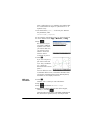
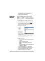
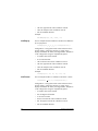
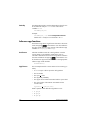
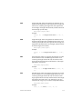
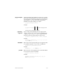
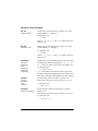
HP Prime Graphing Calculator
User Guide
Edition1
Part Number NW280-2001
Legal Notices
This manual and any examples contained herein are provided "as is" and are subject to
change without notice. Hewlett-Packard Company makes no warranty of any kind with regard
to this manual, including, but not limited to, the implied warranties of merchantability, noninfringement and fitness for a particular purpose.
Portions of this software are copyright 2013 The FreeType Project (www.freetype.org). All rights
reserved.
•
HP is distributing FreeType under the FreeType License.
•
HP is distributing google-droid-fonts under the Apache Software License v2.0.
•
HP is distributing HIDAPI under the BSD license only.
•
HP is distributing Qt under the LGPLv2.1 license. HP is providing a full copy of the Qt
source.
•
HP is distributing QuaZIP under LGPLv2 and the zlib/libpng licenses. HP is providing a full
copy of the QuaZIP source.
Hewlett-Packard Company shall not be liable for any errors or for incidental or consequential
damages in connection with the furnishing, performance, or use of this manual or the examples contained herein.
Product Regulatory & Environment Information
Product Regulatory and Environment Information is provided on the CD shipped with this
product.
Copyright © 2013 Hewlett-Packard Development Company, L.P.
Reproduction, adaptation, or translation of this manual is prohibited without prior written permission of Hewlett-Packard Company, except as allowed under the copyright laws.
Printing History
Edition 1
July 2013
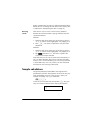
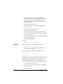
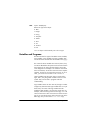
Contents
Preface
Manual conventions ................................................................ 9
Notice ................................................................................. 10
1 Getting started
Before starting ...................................................................... 11
On/off, cancel operations...................................................... 12
The display .......................................................................... 13
Sections of the display ...................................................... 14
Navigation........................................................................... 16
Touch gestures ................................................................. 17
The keyboard ....................................................................... 18
Context-sensitive menu ...................................................... 19
Entry and edit keys................................................................ 20
Shift keys......................................................................... 22
Adding text...................................................................... 23
Math keys ....................................................................... 24
Menus ................................................................................. 28
Toolbox menus................................................................. 29
Input forms ........................................................................... 29
System-wide settings .............................................................. 30
Home settings .................................................................. 30
Specifying a Home setting ................................................. 35
Mathematical calculations ...................................................... 36
Choosing an entry type ..................................................... 36
Entering expressions ......................................................... 37
Reusing previous expressions and results ............................. 40
Storing a value in a variable.............................................. 42
Complex numbers ................................................................. 44
Sharing data ........................................................................ 44
Online Help ......................................................................... 46
2 Reverse Polish Notation (RPN)
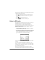
History in RPN mode ............................................................. 48
Sample calculations............................................................... 49
Manipulating the stack........................................................... 51
3 Computer algebra system (CAS)
CAS view............................................................................. 53
CAS calculations................................................................... 54
Settings................................................................................ 55
Contents
1
4 Exam Mode
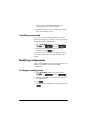
Modifying the default configuration..................................... 62
Creating a new configuration ............................................. 63
Activating Exam Mode ........................................................... 64
Cancelling exam mode...................................................... 66
Modifying configurations........................................................ 66
To change a configuration ................................................. 66
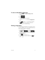
To return to the default configuration ................................... 67
Deleting configurations ...................................................... 67
5 An introduction to HP apps
Application Library ................................................................ 71
App views ............................................................................ 73
Symbolic view .................................................................. 73
Symbolic Setup view ......................................................... 74
Plot view .......................................................................... 75
Plot Setup view ................................................................. 76
Numeric view................................................................... 77
Numeric Setup view .......................................................... 78
Quick example...................................................................... 79
Common operations in Symbolic view...................................... 81
Symbolic view: Summary of menu buttons............................ 86
Common operations in Symbolic Setup view............................. 87
Common operations in Plot view ............................................ 88
Zoom .............................................................................. 88
Trace............................................................................... 94
Plot view: Summary of menu buttons.................................... 96
Common operations in Plot Setup view..................................... 96
Configure Plot view ........................................................... 96
Common operations in Numeric view .................................... 100
Zoom ............................................................................ 100
Evaluating...................................................................... 102
Custom tables................................................................. 103
Numeric view: Summary of menu buttons........................... 104
Common operations in Numeric Setup view............................ 105
Combining Plot and Numeric Views....................................... 106
Adding a note to an app...................................................... 106
Creating an app.................................................................. 107
App functions and variables ................................................. 109
2
Contents
6 Function app
Getting started with the Function app .................................... 111
Analyzing functions ............................................................. 118
The Function Variables......................................................... 122
Summary of FCN operations ................................................ 124
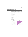
7 Advanced Graphing app
Getting started with the Advanced Graphing app ................... 126
Plot Gallery ........................................................................ 134
Exploring a plot from the Plot Gallery................................ 134
8 Geometry
Getting started with the Geometry app .................................. 135
Plot view in detail................................................................ 141
Plot Setup view............................................................... 146
Symbolic view in detail ........................................................ 148
Symbolic Setup view....................................................... 150
Numeric view in detail ........................................................ 150
Geometric objects ............................................................... 153
Geometric transformations ................................................... 161
Geometry functions and commands....................................... 165
Symbolic view: Cmds menu ............................................. 165
Numeric view: Cmds menu.............................................. 182
Other Geometry functions................................................ 189
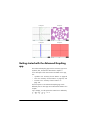
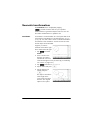
9 Spreadsheet
Getting started with the Spreadsheet app............................... 195
Basic operations ................................................................. 199
Navigation, selection and gestures ................................... 199
Cell references ............................................................... 200
Cell naming ................................................................... 200
Entering content ............................................................. 201
Copy and paste ............................................................. 204
External references .............................................................. 204
Referencing variables...................................................... 205
Using the CAS in spreadsheet calculations ............................. 206
Buttons and keys ................................................................. 207
Formatting options .............................................................. 208
Spreadsheet functions .......................................................... 210
10 Statistics 1Var app
Getting started with the Statistics 1Var app ............................ 211
Entering and editing statistical data ....................................... 215
Computed statistics.............................................................. 218
Plotting .............................................................................. 219
Contents
3
Plot types ....................................................................... 219
Setting up the plot (Plot Setup view)................................... 221
Exploring the graph ........................................................ 221
11 Statistics 2Var app
Getting started with the Statistics 2Var app............................. 223
Entering and editing statistical data ....................................... 228
Numeric view menu items ................................................ 229
Defining a regression model ................................................. 231
Computed statistics .............................................................. 233
Plotting statistical data.......................................................... 234
Plot view: menu items ...................................................... 236
Plot setup ....................................................................... 236
Predicting values............................................................. 237
Troubleshooting a plot ..................................................... 238
12 Inference app
Getting started with the Inference app.................................... 239
Importing statistics ............................................................... 243
Hypothesis tests ................................................................... 245
One-Sample Z-Test .......................................................... 246
Two-Sample Z-Test .......................................................... 247
One-Proportion Z-Test ...................................................... 248
Two-Proportion Z-Test ...................................................... 249
One-Sample T-Test .......................................................... 250
Two-Sample T-Test ........................................................... 251
Confidence intervals ............................................................ 253
One-Sample Z-Interval ..................................................... 253
Two-Sample Z-Interval...................................................... 253
One-Proportion Z-Interval ................................................. 254
Two-Proportion Z-Interval.................................................. 255
One-Sample T-Interval...................................................... 256
Two-Sample T-Interval ...................................................... 256
13 Solve app
Getting started with the Solve app ......................................... 259
One equation ................................................................. 260
Several equations ........................................................... 263
Limitations...................................................................... 264
Solution information ............................................................. 265
14 Linear Solver app
Getting started with the Linear Solver app............................... 267
Menu items ......................................................................... 269
4
Contents
15 Parametric app
Getting started with the Parametric app ................................. 271
16 Polar app
Getting started with the Polar app ......................................... 277
17 Sequence app
Getting started with the Sequence app .................................. 281
Another example: Explicitly-defined sequences ....................... 285
18 Finance app
Getting Started with the Finance app..................................... 287
Time value of money (TVM) .................................................. 290
TVM calculations: Another example....................................... 291
Calculating amortizations..................................................... 293
19 Triangle Solver app
Getting started with the Triangle Solver app ........................... 295
Choosing triangle types ....................................................... 297
Special cases ..................................................................... 298
20 The Explorer apps
Linear Explorer app............................................................. 299
Quadratic Explorer app ....................................................... 302
Trig Explorer app ................................................................ 304
21 Functions and commands
Keyboard functions ............................................................. 309
Math menu......................................................................... 313
Numbers ....................................................................... 313
Arithmetic ...................................................................... 314
Trigonometry.................................................................. 316
Hyperbolic .................................................................... 317
Probability ..................................................................... 317
List................................................................................ 322
Matrix........................................................................... 323
Special ......................................................................... 323
CAS menu.......................................................................... 324
Algebra ........................................................................ 324
Calculus ........................................................................ 326
Solve ............................................................................ 330
Rewrite.......................................................................... 332
Integer .......................................................................... 337
Polynomial..................................................................... 339
Plot ............................................................................... 346
Contents
5
App menu .......................................................................... 347
Function app functions..................................................... 348
Solve app functions ......................................................... 349
Spreadsheet app functions ............................................... 349
Statistics 1Var app functions............................................. 363
Statistics 2Var app functions............................................. 365
Inference app functions.................................................... 366
Finance app functions ..................................................... 372
Linear Solver app functions .............................................. 374
Triangle Solver app functions ........................................... 374
Linear Explorer functions .................................................. 376
Quadratic Explorer functions ............................................ 377
Common app functions.................................................... 377
Ctlg menu........................................................................... 378
Creating your own functions ................................................. 421
22 Variables
Qualifying variables ............................................................ 427
Home variables ................................................................... 428
App variables ..................................................................... 429
Function app variables .................................................... 429
Geometry app variables .................................................. 430
Spreadsheet app variables............................................... 431
Solve app variables ........................................................ 431
Advanced Graphing app variables ................................... 432
Statistics 1Var app variables ............................................ 433
Statistics 2Var app variables ............................................ 435
Inference app variables ................................................... 437
Parametric app variables ................................................. 439
Polar app variables......................................................... 440
Finance app variables ..................................................... 440
Linear Solver app variables .............................................. 441
Triangle Solver app variables ........................................... 441
Linear Explorer app variables ........................................... 441
Quadratic Explorer app variables ..................................... 441
Trig Explorer app variables .............................................. 442
Sequence app variables .................................................. 442
23 Units and constants
Units .................................................................................. 443
Unit calculations .................................................................. 444
Unit tools ............................................................................ 446
Physical constants ................................................................ 447
List of constants............................................................... 449
6
Contents
24 Lists
Create a list in the List Catalog ............................................. 451
The List Editor................................................................. 453
Deleting lists ....................................................................... 455
Lists in Home view............................................................... 455
List functions ....................................................................... 457
Finding statistical values for lists ............................................ 461
25 Matrices
Creating and storing matrices............................................... 464
Working with matrices......................................................... 465
Matrix arithmetic................................................................. 469
Solving systems of linear equations ....................................... 472
Matrix functions and commands............................................ 474
Matrix functions .................................................................. 475
Examples....................................................................... 486
26 Notes and Info
The Note Catalog ............................................................... 489
The Note Editor .................................................................. 490
27 Programming in HP PPL
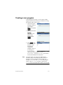
The Program Catalog .......................................................... 498
Creating a new program ..................................................... 501
The Program Editor ......................................................... 502
The HP Prime programming language ................................... 511
The User Keyboard: Customizing key presses .................... 516
App programs ............................................................... 520
Program commands ............................................................ 527
Commands under the Tmplt menu ..................................... 528
Block ............................................................................ 528
Branch .......................................................................... 528
Loop ............................................................................. 529
Variable ........................................................................ 533
Function ........................................................................ 533
Commands under the Cmds menu .................................... 534
Strings .......................................................................... 534
Drawing........................................................................ 536
Matrix........................................................................... 544
App Functions ................................................................ 546
Integer .......................................................................... 547
I/O .............................................................................. 549
More ............................................................................ 554
Variables and Programs .................................................. 556
Contents
7
28 Basic integer arithmetic
The default base.................................................................. 582
Changing the default base ............................................... 583
Examples of integer arithmetic............................................... 584
Integer manipulation ............................................................ 585
Base functions ..................................................................... 586
A Glossary
B Troubleshooting
Calculator not responding .................................................... 591
To reset ......................................................................... 591
If the calculator does not turn on ....................................... 591
Operating limits .................................................................. 592
Status messages .................................................................. 592
C Product regulatory information
Federal Communications Commission notice........................... 595
European Union Regulatory Notice ........................................ 597
Index
8
................................................................................... 601
Contents
Preface
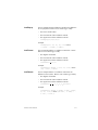
Manual conventions
The following conventions are used in this manual to
represent the keys that you press and the menu options
that you choose to perform operations.
•
A key that initiates an unshifted function is
represented by an image of that key:
e,B,H, etc.
•
A key combination that initiates a shifted unction (or
inserts a character) is represented by the appropriate
shift key (S or A) followed by the key for that
function or character:
Sh initiates the natural exponential function
and Az inserts the pound character (#)
The name of the shifted function may also be given in
parentheses after the key combination:
SJ(Clear), SY (Setup)
•
A key pressed to insert a digit is represented by that
digit:
5, 7, 8, etc.
•
All fixed on-screen text—such as screen and field
names—appear in bold:
CAS Settings, XSTEP, Decimal Mark, etc.
•
A menu item selected by touching the screen is
represented by an image of that item:
,
,
.
Note that you must use your finger to select a menu
item. Using a stylus or something similar will not
select whatever is touched.
Preface
9
•
Items you can select from a list, and characters on the
entry line, are set in a non-proportional font, as
follows:
Function, Polar, Parametric, Ans, etc.
•
Cursor keys are represented by =, \, >, and <.
You use these keys to move from field to field on a
screen, or from one option to another in a list of
options.
•
Error messages are enclosed in quotation marks:
“Syntax Error”
Notice
This manual and any examples contained herein are
provided as-is and are subject to change without notice.
Except to the extent prohibited by law, Hewlett-Packard
Company makes no express or implied warranty of any
kind with regard to this manual and specifically disclaims
the implied warranties and conditions of merchantability
and fitness for a particular purpose and Hewlett-Packard
Company shall not be liable for any errors or for
incidental or consequential damage in connection with
the furnishing, performance or use of this manual and the
examples herein.
1994–1995, 1999–2000, 2003–2006, 2010–2013
Hewlett-Packard Development Company, L.P.
The programs that control your HP Prime are copyrighted
and all rights are reserved. Reproduction, adaptation, or
translation of those programs without prior written
permission from Hewlett-Packard Company is also
prohibited.
For hardware warranty information, please refer to the
HP Prime Quick Start Guide.
Product Regulatory and Environment Information is
provided on the CD shipped with this product.
10
Preface
1
Getting started
The HP Prime Graphing Calculator is an easy-to-use yet
powerful graphing calculator designed for secondary
mathematics education and beyond. It offers hundreds of
functions and commands, and includes a computer
algebra system (CAS) for symbolic calculations.
In addition to an extensive library of functions and
commands, the calculator comes with a set of HP apps.
An HP app is a special application designed to help you
explore a particular branch of mathematics or to solve a
problem of a particular type. For example, there is a HP
app that will help you explore geometry and another to
help you explore parametric equations. There are also
apps to help you solve systems of linear equations and to
solve time-value-of-money problems.
The HP Prime also has its own programming language
you can use to explore and solve mathematical problems.
Functions, commands, apps and programming are
covered in detail later in this guide. In this chapter, the
general features of the calculator are explained, along
with common interactions and basic mathematical
operations.
Before starting
Charge the battery fully before using the calculator for the
first time. To charge the battery, either:
Getting started
•
Connect the calculator to a computer using the USB
cable that came in the package with your HP Prime.
(The PC needs to be on for charging to occur.)
•
Connect the calculator to a wall outlet using the HPprovided wall adapter.
11
When the calculator is on, a battery symbol appears in
the title bar of the screen. Its appearance will indicate how
much power the battery has. A flat battery will take
approximately 4 hours to become fully charged.
Battery Warning
Adapter Warning
•
To reduce the risk of fire or burns, do not
disassemble, crush or puncture the battery; do not
short the external contacts; and do not dispose of the
battery in fire or water.
•
To reduce potential safety risks, only use the battery
provided with the calculator, a replacement battery
provided by HP, or a compatible battery
recommended by HP.
•
Keep the battery away from children.
•
If you encounter problems when charging the
calculator, stop charging and contact HP
immediately.
•
To reduce the risk of electric shock or damage to
equipment, only plug the AC adapter into an AC
outlet that is easily accessible at all times.
•
To reduce potential safety risks, only use the AC
adapter provided with the calculator, a replacement
AC adapter provided by HP, or an AC adapter
purchased as an accessory from HP.
On/off, cancel operations
To turn on
Press O to turn on the calculator.
To cancel
When the calculator is on, pressing the J key cancels
the current operation. For example, it will clear whatever
you have entered on the entry line. It will also close a
menu and a screen.
To turn off
Press SO(Off) turn the calculator off.
To save power, the calculator turns itself off after several
minutes of inactivity. All stored and displayed information
is saved.
12
Getting started
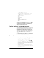
The Home View
Home view is the starting point for many calculations.
Most mathematical functions are available in the Home
view. Some additional functions are available in the
computer algebra system (CAS). A history of your
previous calculations is retained and you can re-use a
previous calculation or its result.
To display Home view, pressH.
The CAS View
CAS view enables you to perform symbolic calculations. It
is largely identical to Home view—it even has its own
history of past calculations—but the CAS view offers some
additional functions.
To display CAS view, pressK.
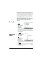
Protective cover
The calculator is provided with a slide cover to protect the
display and keyboard. Remove the cover by grasping
both sides of it and pulling down.
You can reverse the slide cover and slide it onto the back
of the calculator. This will ensure that you do not misplace
the cover while you are using the calculator.
To prolong the life of the calculator, always place the
cover over the display and keyboard when you are not
using the calculator.
The display
To adjust the
brightness
To adjust the brightness of the display, press and hold
O, then press the + or w key to increase or
decrease the brightness. The brightness will change with
each press of the + or w key.
To clear the display
•
Press J or O to clear the entry line.
•
Press SJ (Clear) to clear the entry line and the
history.
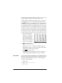
Getting started
13
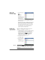
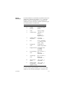
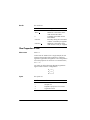
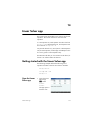
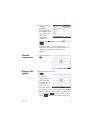
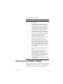
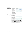
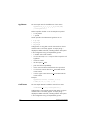
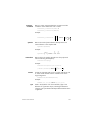
Sections of the display
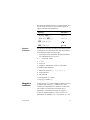
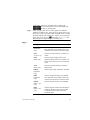
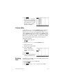
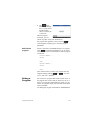
Title bar
History
Entry line
Menu buttons
Home view has four sections (shown above). The title bar
shows either the screen name or the name of the app you
are currently using—Function in the example above. It
also shows the time, a battery power indicator, and a
number of symbols that indicate various calculator
settings. These are explained below. The history displays
a record of your past calculations. The entry line
displays the object you are currently entering or
modifying. The menu buttons are options that are
relevant to the current display. These options are selected
by tapping the corresponding menu button. You close a
menu, without making a selection from it, by pressing
J.
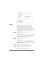
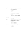
Annunciators. Annunciators are symbols or characters
that appear in the title bar. They indicate current settings,
and also provide time and battery power information.
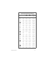
Annunciator
[Lime green]
π
[Lime green]
S [Cyan]
14
Meaning
The angle mode setting is currently
degrees.
The angle mode setting is currently
radians.
The Shift key is active. The function
shown in blue on a key will be
activated when a key is pressed.
Press S to cancel shift mode.
Getting started
Getting started
Annunciator
Meaning (Continued)
CAS [White]
You are working in CAS view, not
Home view.
A...Z [orange]
In Home view
The Alpha key is active. The character shown in orange on a key will
be entered in uppercase when a
key is pressed. See “Adding text”
on page 23 for more information.
In CAS view
The Alpha–Shift key combination is
active. The character shown in
orange on a key will be entered in
uppercase when a key is pressed.
See “Adding text” on page 23 for
more information.
a...z [orange]
In Home view
The Alpha–Shift key combination is
active. The character shown in
orange on a key will be entered in
lowercase when a key is pressed.
See “Adding text” on page 23 for
more information.
In CAS view
The Alpha key is active. The character shown in orange on a key will
be entered in lowercase when a key
is pressed. See “Adding text” on
page 23 for more information.
U [Yellow]
The user keyboard is active. All the
following key presses will enter the
customized objects associated with
the key. See “The User Keyboard:
Customizing key presses” on page
516 for more information.
15
Annunciator
1U
[Yellow]
[Time]
[Green with
gray border]
Meaning (Continued)
The user keyboard is active. The
next key press will enter the customized object associated with the key.
See “The User Keyboard: Customizing key presses” on page 516 for
more information.
Current time. The default is 24-hour
format, but you can choose AM–PM
format. See “Home settings” on
page 30 for more information.
Battery-charge indicator.
Navigation
The HP Prime offers two modes of navigation: touch and
keys. In many cases, you can tap on an icon, field, menu,
or object to select (or deselect) it. For example, you can
open the Function app by tapping once on its icon in the
Application Library. However, to open the Application
Library, you will need to press a key: I.
Instead of tapping an icon in the Application Library, you
can also press the cursor keys—=,\,<,>—until the
app you want to open is highlighted, and then press
E. In the Application Library, you can also type the
first one or two letters of an app’s name to highlight the
app. Then either tap the app’s icon or press E to
open it.
Sometimes a touch or key–touch combination is available.
For example, you can deselect a toggle option either by
tapping twice on it, or by using the arrow keys to move to
the field and then tapping a touch button along the bottom
of the screen (in this case
).
Note that you must use your finger or a capacitive stylus
to select an item by touch.
16
Getting started
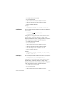
Touch gestures
In addition to selection by tapping, there are other touchrelated operations available to you:
To quickly move from page to page, flick:
Place a finger on the screen and quickly swipe it in the
desired direction (up or down).
To pan, drag your finger horizontally or vertically across
the screen.
To quickly zoom in, make an open pinch:
Place the thumb and a finger close together on the
screen and move them apart. Only lift them from the
screen when you reach the desired magnification.
To quickly zoom out, make an closed pinch:
Place the thumb and a finger some distance apart on
the screen and move them toward each other. Only lift
them from the screen when you reach the desired
magnification.
Note that pinching to zoom only works in applications
that feature zooming (such as where graphs are plotted).
In other applications, pinching will do nothing, or do
something other than zooming. For example, in the
Spreadsheet app, pinching will change the width of a
column or the height of a row.
Getting started
17
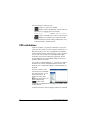
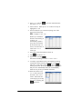
The keyboard
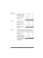
The numbers in the legend below refer to the parts of the
keyboard described in the illustration on the next page.
Number Feature
18
1
LCD and touch-screen: 320 × 240 pixels
2
Context-sensitive touch-button menu
3
HP Apps keys
4
Home view and preference settings
5
Common math and science functions
6
Alpha and Shift keys
7
On, Cancel and Off key
8
List, matrix, program, and note catalogs
9
Last Answer key (Ans)
10
Enter key
11
Backspace and Delete key
12
Menu (and Paste) key
13
CAS (and CAS preferences) key
14
View (and Copy) key
15
Escape (and Clear) key
16
Help key
17
Rocker wheel (for cursor movement)
Getting started
1
2
17
16
3
4
5
15
14
13
12
11
10
6
7
9
8
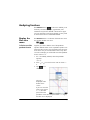
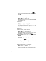
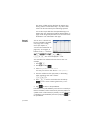
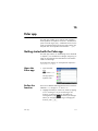
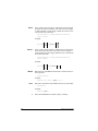
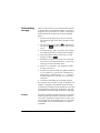
Context-sensitive menu
A context-sensitive menu occupies the bottom line of the
screen.
The options available depend on the context, that is, the
view you are in. Note that the menu items are activated by
touch.
Getting started
19
There are two types of buttons on the context-sensitive
menu:
•
menu button: tap to display a pop-up menu. These
buttons have square corners along their top (such as
in the illustration above).
•
command button: tap to initiate a command. These
buttons have rounded corners (such as
in the
illustration above).
Entry and edit keys
The primary entry and edit keys are:
20
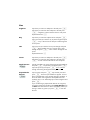
Keys
Purpose
N to r
Enter numbers
O or J
Cancels the current operation or
clears the entry line.
E
Enters an input or executes an
operation. In calculations, E
acts like “=”. When
or
is present as a menu key,
E acts the same as pressing
or
.
Q
For entering a negative number. For
example, to enter –25, press
Q25. Note: this is not the same
operation that is performed by the
subtraction key (w).
F
Math template: Displays a palette
of pre-formatted templates representing common arithmetic expressions.
d
Enters the independent variable
(that is, either X, T, or N, depending on the app that is currently
active).
Getting started
Getting started
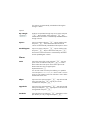
Keys
Purpose (Continued)
Sv
Relations palette: Displays a palette
of comparison operators and Boolean operators.
Sr
Special symbols palette: Displays a
palette of common math and Greek
characters.
Sc
Automatically inserts the degree,
minute, or second symbol according to the context.
C
Backspace. Deletes the character to
the left of the cursor. It will also
return the highlighted field to its
default value, if it has one.
SC
Delete. Deletes the character to the
right of the cursor.
SJ(Clear)
Clears all data on the screen
(including the history). On a settings screen—for example Plot
Setup—returns all settings to their
default values.
<>=\
Cursor keys: Moves the cursor
around the display. Press S\ to
move to the end of a menu or
screen, or S= to move to the
start. (These keys represent the
directions of the rocker wheel.)
21
Keys
Purpose (Continued)
Sa
Displays all the available
characters. To enter a character, use
the cursor keys to highlight it, and
then tap
. To select multiple
characters, select one, tap
,
and continue likewise before
pressing
. There are many
pages of characters. You can jump
to a particular Unicode block by
tapping
and selecting the
block. You can also flick from page
to page.
Shift keys
There are two shift keys that you use to access the
operations and characters printed on the bottom of the
keys: S and A.
22
Key
Purpose
S
Press S to access the operations
printed in blue on a key. For
instance, to access the settings for
Home view, press SH.
A
Press the A key to access the
characters printed in orange on a
key. For instance, to type Z in Home
view, press A and then press
y. For a lowercase letter, press
AS and then the letter. In CAS
view, A and another key gives a
lowercase letter, and AS and
another letter gives an uppercase
letter.
Getting started
Adding text
The text you can enter directly is shown by the orange
characters on the keys. These characters can only be
entered in conjunction with the A and S keys. Both
uppercase and lowercase characters can be entered, and
the method is exactly the opposite in CAS view than in
Home view.
Keys
Effect in Home view
Effect in CAS view
A
Makes the next character uppercase
Makes the next character lowercase
AA Lock mode: makes all
characters uppercase
until the mode is reset
S
Lock mode: makes all
characters lowercase until
the mode is reset
With uppercase locked, With lowercase locked,
makes the next character makes the next character
uppercase
lowercase
AS Makes the next character lowercase
Makes the next character uppercase
Lock mode: makes all
AS Lock mode: makes all
characters lowercase until characters uppercase
A
until the mode is reset
the mode is reset
S
With lowercase locked, With uppercase locked,
makes the next character makes the next character
lowercase
uppercase
With uppercase locked,
makes all characters lowmakes all characters
uppercase until the mode ercase until the mode is
reset
is reset
SA With lowercase locked,
Reset uppercase lock
mode
Reset lowercase lock
mode
AA Reset lowercase lock
mode
AA
Reset uppercase lock
mode
A
You can also enter text (and other characters) by
displaying the characters palette: Sa.
Getting started
23
Math keys
The most common math functions have their own keys on
the keyboard (or a key in combination with the S key).
Example 1: To calculate SIN(10), press e10 and
press E. The answer displayed is –0.544… (if your
angle measure setting is radians).
Example 2: To find the square root of 256, press
Sj 256 and press E. The answer displayed
is 16. Notice that the S key initiates the operator
represented in blue on the next key pressed (in this case √
on the j key).
The mathematical functions not represented on the keyboard
are on the Math, CAS, and Catlg menus (see chapter 21,
“Functions and commands”, starting on page 307).
Note that the order in which you enter operands and
operators is determined by the entry mode. By default, the
entry mode is textbook, which means that you enter
operands and operators just as you would if you were
writing the expression on paper. If your preferred entry
mode is Reverse Polish Notation, the order of entry is
different. (See chapter 2, “Reverse Polish Notation (RPN)”,
starting on page 47.)
Math
template
24
The math template key (F)
helps you insert the framework
for common calculations (and for
vectors, matrices, and
hexagesimal numbers). It
displays a palette of pre-formatted outlines to which you
add the constants, variables, and so on. Just tap on the
template you want (or use the arrow keys to highlight it
and press E). Then enter the components needed
to complete the calculation.
Getting started
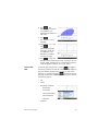
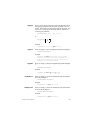
Example: Suppose you want to find the cube root of
945:
1. In Home view, press F.
2. Select
.
The skeleton or framework for your calculation now
appears on the entry line:
3. Each box on the template needs to be completed:
3>945
4. Press E to display the result: 9.813…
The template palette can save you a lot of time, especially
with calculus calculations.
You can display the palette at any stage in defining an
expression. In other words, you don’t need to start out with
a template. Rather, you can embed one or more templates
at any point in the definition of an expression.
Math
shortcuts
As well as the math template,
there are other similar screens
that offer a palette of special
characters. For example,
pressing Sr displays the
special symbols palette, shown at the right. Select a
character by tapping it (or scrolling to it and pressing
E).
A similar palette—the relations
palette—is displayed if you press
Sv. The palette displays operators
useful in math and programming. Again,
just tap the character you want.
Other math shortcut keys include d. Pressing this key
inserts an X, T, , or N depending on what app you are
using. (This is explained further in the chapters describing
the apps.)
Similarly, pressing Sc enters a degree, minute, or
second character. It enters ° if no degree symbol is part of
your expression; enters ′ if the previous entry is a value in
Getting started
25
degrees; and enters ″ if the previous entry is a value in
minutes. Thus entering:
36Sc40Sc20Sc
yields 36°40′20″. See “Hexagesimal numbers” on page
26 for more information.
Fractions
The fraction key (c) cycles through thee varieties of
fractional display. If the current answer is the decimal
fraction 5.25, pressing c converts the answer to the
common fraction 21/4. If you press c again, the
answer is converted to a mixed number (5 + 1/4). If
pressed again, the display returns to the decimal fraction
(5.25).
The HP Prime will
approximate fraction and
mixed number
representations in cases
where it cannot find
exact ones. For example,
enter 5 to see the
decimal approximation:
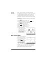
------------------ and again to see
2.236…. Press c once to see 219602
98209
23184
2 + --------------- . Pressing c a third time will cycle back to the
98209
original decimal representation.
Hexagesimal
numbers
Any decimal result can de displayed in hexagesimal
format; that is, in units subdivided into groups of 60. This
includes degrees, minutes, and seconds as well as hours,
------ to see the
minutes, and seconds. For example, enter 11
8
decimal result: 1.375. Now press S c to see
1°22′ 30. Press S c again to return to the decimal
representation.
HP Prime will produce the best approximation in cases
where an exact result is not possible. Enter 5 to see the
decimal approximation: 2.236… Press S c to see
2°14′ 9.84472.
26
Getting started
Note that the degree and minute entries must be integers,
and the minute and second entries must be positive.
Decimals are not allowed, except in the seconds.
Note too that the HP
Prime treats a value in
hexgesimal format as a
single entity. Hence any
operation performed on
a hexagesimal value is
performed on the entire
value. For example, if
you enter 10°25′ 26″ 2, the whole value is squared, not just
the seconds component. The result in this case is
108°39′ 26.8544″ .
EEX key
(powers of
10)
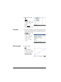
Numbers like 5 10 4 and 3.21 10–7 are expressed in
scientific notation, that is, in terms of powers of ten. This is
simpler to work with than 50 000 or 0.000 000 321. To
enter numbers like these, use the B functionality. This is
easier than using s10k.
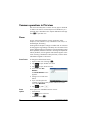
Example: Suppose you want to calculate
– 13
23
4 10 6 10
---------------------------------------------------–5
3 10
First select Scientific as the number format.
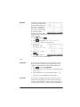
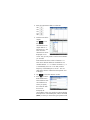
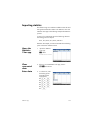
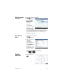
1. Open the Home Settings window.
SH
2. Select Scientific
from the Number
Format menu.
3. Return home: H
4. Enter 4BQ13
s 6B23n
3BQ5
Getting started
27
5. Press E
The result is
8.0000E15. This is
equivalent to
8 × 10¹⁵.
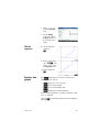
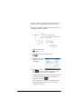
Menus
A menu offers you a
choice of items. As in the
case shown at the right,
some menus have submenus and sub-submenus.
To select from a
menu
There are two techniques for selecting an item from a
menu:
•
direct tapping and
•
using the arrow keys to highlight the item you want
and then either tapping
or pressing E.
Note that the menu of buttons along the bottom of the
screen can only be activated by tapping.
Shortcuts
28
•
Press = when you are at the top of the menu to
immediately display the last item in the menu.
•
Press \ when you are at the bottom of the menu to
immediately display the first item in the menu.
•
Press S\ to jump straight to the bottom of the
menu.
•
Press S= to jump straight to the top of the menu.
•
Enter the first few characters of the item’s name to
jump straight to that item.
•
Enter the number of the item shown in the menu to
jump straight to that item.
Getting started
To close a menu
A menu will close automatically when you select an item
from it. If you want to close a menu without selecting
anything from it, press O or J.
Toolbox menus
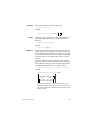
The Toolbox menus (D) are a collection of menus
offering functions and commands useful in mathematics
and programming. The Math, CAS, and Catlg menus
offer over 400 functions and commands. The items on
these menus are described in detail in chapter 21,
“Functions and commands”, starting on page 307.
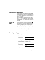
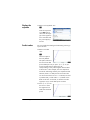
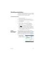
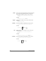
Input forms
An input form is a screen that provides one or more fields
for you to enter data or select an option. It is another name
for a dialog box.
•
If a field allows you to enter data of your choice, you
can select it, add your data, and tap
. (There
is no need to tap
first.)
•
If a field allows you to choose an item from a menu,
you can tap on it (the field or the label for the field),
tap on it again to display the options, and tap on the
item you want. (You can also choose an item from an
open list by pressing the cursor keys and pressing
E when the option you want is highlighted.)
•
If a field is a toggle field—one that is either selected
or not selected—tap on it to select the field and tap
on it again to select the alternate option.
(Alternatively, select the field and tap
.)
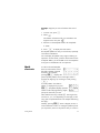
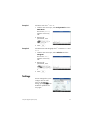
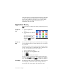
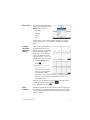
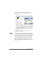
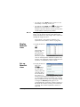
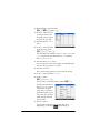
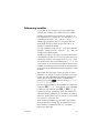
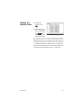
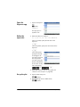
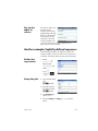
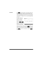
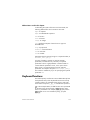
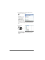
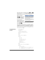
The illustration at the right
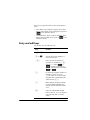
shows an input form with
all three types of field:
Calculator Name is a
free-form data-entry field,
Font Size provides a
menu of options, and
Textbook Display is a
toggle field.
Getting started
29
Reset input
form fields
To reset a field to its default value, highlight the field and
press
. To reset all fields to their default values, press
SJ (Clear).
C
System-wide settings
System-wide settings are values that determine the
appearance of windows, the format of numbers, the scale
of plots, the units used by default in calculations, and
much more.
There are two system-wide settings: Home settings and
CAS settings. Home settings control Home view and the
apps. CAS settings control how calculations are done in
the computer algebra system. CAS settings are discussed
in chapter 3.
Although Home settings control the apps, you can
override certain Home settings once inside an app. For
example, you can set the angle measure to radians in the
Home settings but choose degrees as the angle measure
once inside the Polar app. Degrees then remains the angle
measure until you open another app that has a different
angle measure.
Home settings
You use the Home
Settings input form to
specify the settings for
Home view (and the
default settings for the
apps). Press SH
(Settings) to open the
Home Settings input
form. There are four pages of settings.
30
Getting started
Page 1
Setting
Options
Angle Measure
Degrees: 360 degrees in a circle.
Radians: 2 radians in a circle.
The angle mode you set is the angle
setting used in both Home view and
the current app. This is to ensure
that trigonometric calculations done
in the current app and Home view
give the same result.
Number
Format
The number format you set is the format used in all Home view calculations.
Standard: Full-precision display.
Fixed: Displays results rounded to
a number of decimal places. If you
choose this option, a new field
appears for you to enter the number
of decimal places. For example,
123.456789 becomes 123.46 in
Fixed 2 format.
Scientific: Displays results with an
one-digit exponent to the left of the
decimal point, and the specified
number of decimal places. For
example, 123.456789 becomes
1.23E2 in Scientific 2
format.
Engineering: Displays results with
an exponent that is a multiple of 3,
and the specified number of
significant digits beyond the first
one. Example: 123.456E7
becomes 1.23E9 in Engineering 2 format.
Getting started
31
Setting
Options (Continued)
Entry
Textbook: An expression is
entered in much the same way as if
you were writing it on paper (with
some arguments above or below
others). In other words, your entry
could be two-dimensional.
Algebraic: An expression is
entered on a single line. Your entry
is always one-dimensional.
RPN: Reverse Polish Notation. The
arguments of the expression are
entered first followed by the
operator. The entry of an operator
automatically evaluates what has
already been entered.
Integers
Sets the default base for integer
arithmetic: binary, octal, decimal,
or hex. You can also set the number
of bits per integer and whether integers are to be signed.
Complex
Choose one of two formats for
displaying complex numbers:
(a,b) or a+b*i.
To the right of this field is an
unnamed checkbox. Check it if you
want to allow complex output from
real input.
Language
32
Choose the language you want for
menus, input forms, and the online
help.
Getting started
Setting
Options (Continued)
Decimal Mark
Dot or Comma. Displays a number
as 12456.98 (dot mode) or as
12456,98 (comma mode). Dot
mode uses commas to separate
elements in lists and matrices, and
to separate function arguments.
Comma mode uses semicolons as
separators in these contexts.
Setting
Options
Font Size
Choose between small, medium,
and large font for general display.
Calculator
Name
Enter a name for the calculator.
Textbook
Display
If selected, expressions and results
are displayed in textbook format
(that is, much as you would see in
textbooks). If not selected, expressions and results are displayed in
algebraic format (that is, in onedimensional format). For example,
45
is displayed as [[4,5],[6,2]]
62
in algebraic format.
Menu Display
This setting determines whether the
commands on the Math and CAS
menus are presented descriptively
or in common mathematical
shorthand. The default is to provide
the descriptive names for the
functions. If you prefer the functions
to be presented in mathematical
shorthand, deselect this option.
Page 2
Getting started
33
Setting
Options (Continued)
Time
Set the time and choose a format:
24-hour or AM–PM format. The
checkbox at the far right lets you
choose whether to show or hide the
time on the title bar of screens.
Date
Set the date and choose a format:
YYYY/MM/DD, DD/MM/YYYY, or
MM/DD/YYYY.
Color Theme
Light: black text on a light back-
ground
Dark: white text on a dark back-
ground
At the far right is a option for you to
choose a color for the shading
(such as the color of the highlight).
Page 3
Page 3 of the Home Settings input form is for setting
Exam mode. This mode enables certain functions of the
calculator to be disabled for a set period, with the
disabling controlled by a password. This feature will
primarily be of interest to those who supervise
examinations and who need to ensure that the calculator
is used appropriately by students sitting an examination.
It is described in detail in chapter 4, “Exam Mode”,
starting on page 61.
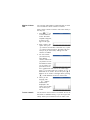
Page 4
Page 4 of the Home Settings input form is for
configuring your HP Prime to work with the HP Prime
Wireless Kit. Visit www.hp.com/support for further
information.
34
Getting started
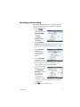
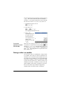
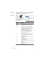
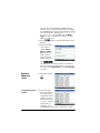
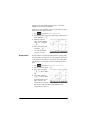
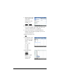
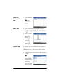
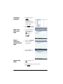
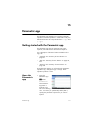
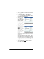
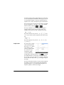
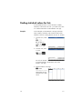
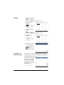
Specifying a Home setting
This example demonstrates how to change the number
format from the default setting—Standard—to Scientific
with two decimal places.
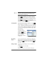
1. Press SH
(Settings) to open the
Home Settings
input form.
The Angle
Measure field is
highlighted.
2. Tap on Number
Format (either the field label or the field). This selects
the field. (You could also have pressed \ to select
it.)
3. Tap on Number
Format again. A
menu of number
format options
appears.
4. Tap on Scientific.
The option is chosen
and the menu closes. (You can also choose an item
by pressing the cursor keys and pressing E
when the option you want is highlighted.)
5. Notice that a number
appears to the right
of the Number
Format field. This is
the number of
decimal places
currently set. To
change the number
to 2, tap on it twice, and then tap on 2 in the menu
that appears.
6. PressHto return to Home view.
Getting started
35
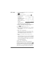
Mathematical calculations
The most commonly used math operations are available
from the keyboard (see “Math keys” on page 24). Access
to the rest of the math functions is via various menus (see
“Menus” on page 28).
Note that the HP Prime represents all numbers smaller
than 1 × 10–499 as zero. The largest number displayed is
9.99999999999 × 10499. A greater result is displayed as
this number.
Where to
start
The home base for the calculator is the Home view (H).
You can do all your non-symbolic calculations here. You
can also do calculations in CAS view, which uses the
computer algebra system (see chapter 3, “Computer
algebra system (CAS)”, starting on page 53). In fact, you
can use functions from the CAS menu (one of the Toolbox
menus) in an expression you are entering in Home view,
and use functions from the Math menu (another of the
Toolbox menus) in an expression you are entering in CAS
view.
Choosing an entry type
The first choice you need to make is the style of entry. The
three types are:
•
Textbook
An expression is
entered in much the
same way as if you
were writing it on paper (with some arguments above
or below others). In other words, your entry could be
two-dimensional, as in the example above.
•
Algebraic
An expression is
entered on a single
line. Your entry is
always one-dimensional.
36
Getting started
•
RPN (Reverse Polish Notation). [Not available in CAS
view.]
The arguments of the expression are entered first
followed by the operator. The entry of an operator
automatically evaluates what has already been
entered. Thus you will need to enter a two-operator
expression (as in the example above) in two steps, one
for each operator:
Step 1: 5 h – the natural logarithm of 5 is
calculated and displayed in history.
Step 2: Szn – is entered as a divisor and
applied to the previous result.
More information about RPN mode can be found in
chapter 2, “Reverse Polish Notation (RPN)”, starting
on page 47.
Note that on page 2 of the Home Settings screen, you
can specify whether you want to display your calculations
in Textbook format or not. This refers to the appearance of
your calculations in the history section of both Home view
and CAS view. This is a different setting from the Entry
setting discussed above.
Entering expressions
The examples that follow assume that the entry mode is
Textbook.
Getting started
•
An expression can contain numbers, functions, and
variables.
•
To enter a function, press the appropriate key, or
open a Toolbox menu and select the function. You
can also enter a function by using the alpha keys to
spell out its name.
•
When you have finished entering the expression,
press E to evaluate it.
37
If you make a mistake while entering an expression, you
can:
Example
•
delete the character to the left of the cursor by
pressing C
•
delete the character to the right of the cursor by
pressing SC
•
clear the entire entry line by pressing O or J.
2
23 – 14 8
Calculate ---------------------------- ln 45
–3
R23jw14S
j8>>nQ3
>h45E
This example illustrates a
number of important
points to be aware of:
Parentheses
38
•
the importance of
delimiters (such as parentheses)
•
how to enter negative numbers
•
the use of implied versus explicit multiplication.
As the example above shows, parentheses are
automatically added to enclose the arguments of
functions, as in LN(). However, you will need to manually
add parentheses—by pressing R—to enclose a group
of objects you want operated on as a single unit.
Parentheses provide a way of avoiding arithmetic
ambiguity. In the example above we wanted the entire
numerator divided by –3, thus the entire numerator was
enclosed in parentheses. Without the parentheses, only
14√8 would have been divided by –3.
Getting started
The following examples show the use of parentheses, and
the use of the cursor keys to move outside a group of
objects enclosed within parentheses.
Algebraic
precedence
Entering ...
Calculates …
e 45+Sz
sin 45 +
e45>+Sz
sin 45 +
Sj85 >s 9
85 9
Sj85s9
85 9
The HP Prime calculates according to the following order
of precedence. Functions at the same level of precedence
are evaluated in order from left to right.
1. Expressions within parentheses. Nested parentheses
are evaluated from inner to outer.
2. !, √, reciprocal, square
3. nth root
n
4. Power, 10
5. Negation, multiplication, division, and modulo
6. Addition and subtraction
7. Relational operators (<, >, ≤, ≥, ==, ≠, =)
8. AND and NOT
9. OR and XOR
10. Left argument of | (where)
11. Assign to variable (:=)
Negative
numbers
It is best to press Q to start a negative number or to insert
a negative sign. Pressing w instead will, in some
situations, be interpreted as an operation to subtract the
next number you enter from the last result. (This is
explained in “To reuse the last result” on page 41.)
To raise a negative number to a power, enclose it in
parentheses. For example, (–5)2 = 25, whereas –52 = –25.
Getting started
39
Explicit and
implied
multiplication
Implied multiplication takes place when two operands
appear with no operator between them. If you enter AB,
for example, the result is A*B. Notice in the example on
page 38 that we entered 14Sk8 without the
multiplication operator after 14. For the sake of clarity, the
calculator adds the operator to the expression in history,
but it is not strictly necessary when you are entering the
expression. You can, though, enter the operator if you
wish (as was done in the examples on page 39). The
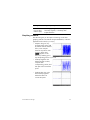
result will be the same.
Large results
If the result is too long or too tall to be seen in its
entirety—for example, a many-rowed matrix—highlight it
and then press
. The result is displayed in fullscreen view. You can now press = and \ (as well as
>and <) to bring hidden parts of the result into view.
Tap
to return to the previous view.
Reusing previous expressions and results
Being able to retrieve and reuse an expression provides a
quick way of repeating a calculation that requires only a
few minor changes to its parameters. You can retrieve and
reuse any expression that is in history. You can also
retrieve and reuse any result that is in history.
To retrieve an expression and place it on the entry line for
editing, either:
•
tap twice on it, or
•
use the cursor keys to highlight the expression and
then either tap on it or tap
.
To retrieve a result and place it on the entry line, use the
cursor keys to highlight it and then tap
.
If the expression or result you want is not showing, press
= repeatedly to step through the entries and reveal those
that are not showing. You can also swipe the screen to
quickly scroll through history.
40
Getting started
Tip
Using the clipboard
Pressing S= takes you straight to the very first entry
in history, and pressing S\ takes you straight to the
most recent entry.
Your last four expressions are always copied to the
clipboard and can easily be retrieved by pressing
SZ. This opens the clipboard from where you can
quickly choose the one you want.
Note that expressions and not results are available from
the clipboard. Note too that the last four expressions
remain on the clipboard even if you have cleared history.
To reuse the last
result
Tip
Press S+ (Ans) to
retrieve your last answer
for use in another
calculation. Ans
appears on the entry
line. This is a shorthand for your last answer and it can be
part of a new expression. You could now enter other
components of a calculation—such as operators, number,
variables, etc.—and create a new calculation.
You don’t need to first select Ans before it can be part of
a new calculation. If you press a binary operator key to
begin a new calculation, Ans is automatically added to
the entry line as the first component of the new
calculation. For example, to multiply the last answer by
13, you could enter S+ s13E. But the
first two keystrokes are unnecessary. All you need to enter
is s13E.
The variable Ans is always stored with full precision
whereas the results in history will only have the precision
determined by the current Number Format setting (see
page 31). In other words, when you retrieve the number
assigned to Ans, you get the result to its full precision; but
when you retrieve a number from history, you get exactly
what was displayed.
Getting started
41
You can repeat the previous calculation simply by pressing
E. This can be useful if the previous calculation
involved Ans. For example, suppose you want to calculate
the nth root of 2 when n is 2, 4, 8, 16, 32, and so on.
1. Calculate the square root of 2.
Sj2E
2. Now enter √Ans.
SjS+E
This calculates the fourth root of 2.
3. Press E
repeatedly. Each time
you press, the root is
twice the previous
root. The last answer
shown in the
illustration at the right
is 32 2 .
To reuse an
expression or result
from the CAS
When your are working in Home view, you can retrieve
an expression or result from the CAS by tapping Z and
selecting Get from CAS. The CAS opens. Press = or
\ until the item you want to retrieve is highlighted and
press E. The highlighted item is copied to the cursor
point in Home view.
Storing a value in a variable
You can store a value in a variable (that is, assign a value
to a variable). Then when you want to use that value in a
calculation, you can refer to it by the variable’s name. You
can create your own variables, or you can take advantage
of the built-in variables in Home view (named A to Z and
) and in the CAS (named a to z, and a few others). CAS
variables can be used in calculations in Home view, and
Home variables can be used in calculations in the CAS.
There are also built-in app variables and geometry
variables. These can also be used in calculations.
42
Getting started
Example: To assign 2 to to the variable A:
Szj
AaE
Your stored value
appears as shown at the
right. If you then wanted
to multiply your stored
value by 5, you could
enter: Aas5E.
You can also create your own variables in Home view. For
example, suppose you wanted to create a variable called
ME and assign 2 to it. You would enter:
Szj
AQAcE
A message appears asking if you want to create a
variable called ME. Tap
or press E to
confirm your intention. You can now use that variable in
subsequent calculations: ME*3 will yield 29.6088132033,
for example.
You can also create variables in CAS view in the same
way. However, the built-in CAS variables must be entered
in lowercase. However, the variables you create yourself
can be uppercase or lowercase.
See chapter 22, “Variables”, starting on page 423 for
more information.
As well as built-in Home and CAS variables, and the
variables you create yourself, each app has variables that
you can access and use in calculations. See “App
functions and variables” on page 109 for more
information.
Getting started
43
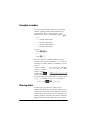
Complex numbers
You can perform arithmetic operations using complex
numbers. Complex numbers can be entered in the
following forms, where x is the real part, y is the
imaginary part, and i is the imaginary constant, – 1 :
•
(x, y)
•
x + yi (except in RPN mode)
•
x – yi (except in RPN mode)
•
x + iy (except in RPN mode), or
•
x – iy (except in RPN mode)
To enter i:
•
press ASg
or
•
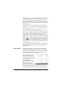
press Sy.
There are 10 built-in variables available for storing
complex numbers. These are labeled Z0 to Z9. You can
also assign a complex number to a variable you create
yourself.
To store a complex
number in a variable,
enter the complex
number, press
,
enter the variable that
you want to assign the complex number to, and then press
E. For example, to store 2+3i in variable Z6:
R2o3>
Ay6E
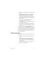
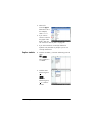
Sharing data
As well as giving you access to many types of
mathematical calculations, the HP Prime enables you to
create various objects that can be saved and used over
and over again. For example, you can create apps, lists,
matrices, programs, and notes. You can also send these
objects to other HP Primes. Whenever you encounter a
44
Getting started
screen with
as a menu item, you can select an item
on that screen to send it to another HP Prime.
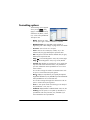
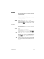
You use one of the
supplied USB cables to
send objects from one
Micro-A: sender
Micro-B: receiver
HP Prime to another.
This is the micro-A–micro B USB cable. Note that the
connectors on the ends of the USB cable are slightly
different. The micro-A connector has a rectangular end
and the micro-B connector has a trapezoidal end. To
share objects with another HP Prime, the micro-A
connector must be inserted into the USB port on the
sending calculator, with the micro-B connector inserted
into the USB port on the receiving calculator.
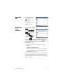
General procedure
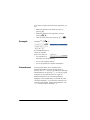
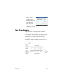
The general procedure for sharing objects is as follows:
1. Navigate to the screen that lists the object you want
to send.
This will be the Application Library for apps, the List
Catalog for lists, the Matrix Catalog for matrices, the
Program Catalog for programs, and the Notes
Catalog for notes.
2. Connect the USB cable between the two calculators.
The micro-A connector—with the rectangular
end—must be inserted into the USB port on the
sending calculator.
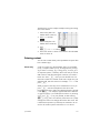
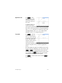
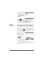
3. On the sending calculator, highlight the object you
want to send and tap
.
In the illustration at
the right, a program
named
TriangleCalcs
has been selected in
the Program Catalog
and will be sent to the
connected calculator
when
is
tapped.
Getting started
45
Online Help
W
Press
to open the online help. The help initially
provided is context-sensitive, that is, it is always about the
current view and its menu items.
For example, to get help on the Function app, press I,
.
select Function, and press
W
From within the help system, tapping
displays a
hierarchical directory of all the help topics. You can
navigate through the directory to other help topics, or use
the search facility to quickly find a topic. You can find help
on any key, view, or command.
46
Getting started
2
Reverse Polish Notation (RPN)
The HP Prime provides you with three ways of entering objects in
Home view:
•
Textbook
An expression is entered in much the same way was if you
were writing it on paper (with some arguments above or
below others). In other words, your entry could be twodimensional, as in the following example:
•
Algebraic
An expression is entered on a single line. Your entry is always
one-dimensional. The same calculation as above would
appear like this is algebraic entry mode:
•
RPN (Reverse Polish Notation).
The arguments of the expression are entered first followed by
the operator. The entry of an operator automatically
evaluates what has already been entered. Thus you will need
to enter a two-operator expression (as in the example above)
in two steps, one for each operator:
Step 1: 5 h – the natural logarithm of 5 is calculated and
displayed in history.
Step 2: Szn – is entered as a divisor and
applied to the previous result.
You choose your preferred entry method from page 1 of the
Home Settings screen (SH). See “System-wide settings”,
starting on page 30 for instructions on how to choose settings.
RPN is available in Home view, but not in CAS view.
Reverse Polish Notation (RPN)
47
The same entry-line editing tools are available in RPN mode as
in algebraic and textbook mode:
•
Press C to delete the character to the left of the cursor.
•
Press SC to delete the character to the right of the
cursor.
•
Press J to clear the entire entry line.
•
Press SJ to clear the entire entry line.
History in RPN mode
The results of your calculations are kept in history. This history is
displayed above the entry line (and by scrolling up to
calculations that are no longer immediately visible). The
calculator offers three histories: one for the CAS view and two for
Home view. CAS history is discussed in chapter 3. The two
histories in Home view are:
•
non-RPN: visible if you have chosen algebraic or textbook
as your preferred entry technique
•
RPN: visible only if you have chosen RPN as your preferred
entry technique. The RPN history is also called the stack. As
shown in the illustration below, each entry in the stack is
given a number. This is the stack level number.
As more calculations are added, an entry’s stack level number
increases.
If you switch from RPN to algebraic or textbook entry, your
history is not lost. It is just not visible. If you switch back to RPN,
your RPN history is redisplayed. Likewise, if you switch to RPN,
your non-RPN history is not lost.
When you are not in RPN mode, your history is ordered
chronologically: oldest calculations at the top, most recent at the
48
Reverse Polish Notation (RPN)
bottom. In RPN mode, your history is ordered chronologically by
default, but you can change the order of the items in history. (This
is explained in “Manipulating the stack” on page 51.)
Re-using
results
There are two ways to re-use a result in history. Method 1
deselects the copied result after copying; method 2 keeps the
copied item selected.
Method 1
1. Select the result to be copied. You can do this by pressing
= or \ until the result is highlighted, or by tapping on it.
2. Press E. The result is copied to the entry line and is
deselected.
Method 2
1. Select the result to be copied. You can do this by pressing
= or \ until the result is highlighted, or by tapping on it.
2. Tap
and select ECHO. The result is copied to the
entry line and remains selected.
Note that while you can copy an item from the CAS history to
use in a Home calculation (and copy an item from the Home
history to use in a CAS calculation), you cannot copy items from
or to the RPN history. You can, however, use CAS commands
and functions when working in RPN mode.
Sample calculations
The general philosophy behind RPN is that arguments are
placed before operators. The arguments can be on the entry line
(each separated by a space) or they can be in history. For
example, to multiply by 3, you could enter:
SzX 3
s
). Thus your
on the entry line and then enter the operator (
entry line would look like this before entering the operator:
Reverse Polish Notation (RPN)
49
However, you could also have entered the arguments separately
and then, with a blank entry line, entered the operator (
).
Your history would look like this before entering the operator:
s
If there are no entries in history and you enter an operator or
function, an error message appears. An error message will also
appear if there is an entry on a stack level that an operator needs
but it is not an appropriate argument for that operator. For
example, pressing f when there is a string on level 1 displays
an error message.
An operator or function will work only on the minimum number of
arguments necessary to produce a result. Thus if you enter on the
entry line 2 4 6 8 and press s, stack level 1 shows 48.
Multiplication needs only two arguments, so the two arguments last
entered are the ones that get multiplied. The entries 2 and 4 are not
ignored: 2 is placed on stack level 3 and 4 on stack level 2.
Where a function can accept a variable number of arguments,
you need to specify how many arguments you want it to include
in its operation. You do this by specifying the number in
parentheses straight after the function name. You then press
E to evaluate the function. For example, suppose your
stack looks like this:
Suppose further that you want to determine the minimum of just
the numbers on stack levels 1, 2, and 3. You choose the MIN
function from the MATH menu and complete the entry as
MIN(3). When you press E, the minimum of just the last
three items on the stack is displayed.
50
Reverse Polish Notation (RPN)
Manipulating the stack
A number of stack-manipulation options are available. Most
appear as menu items across the bottom the screen. To see these
items, you must first select an item in history:
PICK
Copies the selected item to stack level 1. The item below the one
that is copied is then highlighted. Thus if you tapped
four
times, four consecutive items will be moved to the bottom four
stack levels (levels 1–4).
ROLL
There are two roll commads:
•
Tap
to move the selected item to stack level 1. This is
similar to PICK, but PICK duplicates the item, with the
duplicate being placed on stack level1. However, ROLL
doesn’t duplicate an item. It simply moves it.
•
Tap
to move the item on stack level 1 to the currently
highlighted level
Swap
You can swap the position of the objects on stack level 1 with
those on stack level 2. Just press o. The level of other objects
remains unchanged. Note that the entry line must not be active
at the time, otherwise a comma will be entered.
Stack
Tapping
DROPN
displays further stack-manipulation tools.
Deletes all items in the stack from the highlighted item down to
and including the item on stack level 1. Items above the
highlighted item drop down to fill the levels of the deleted items.
If you just want to delete a single item from the stack, see “Delete
an item” below.
Reverse Polish Notation (RPN)
51
DUPN
Duplicates all items between (and including) the highlighted item
and the item on stack level 1. If, for example, you have selected
the item on stack level 3, selecting DUPN duplicates it and the
two items below it, places them on stack levels 1 to 3, and moves
the items that were duplicated up to stack levels 4 to 6.
Echo
Places a copy of the selected result on the entry line and leaves
the source result highlighted.
LIST
Creates a list of results, with the highlighted result the first element
in the list and the item on stack level 1 the last.
Before
After
Show an
item
To show a result in full-screen textbook format, tap
Delete an
item
To delete an item from the stack:
Tap
.
to return to the history.
1. Select it. You can do this by pressing = or \ until the item
is highlighted, or by tapping on it.
2. Press C.
Delete all
items
52
To delete all items, thereby clearing the history, press SJ.
Reverse Polish Notation (RPN)
3
Computer algebra system (CAS)
A computer algebra system (CAS) enables you to perform
symbolic calculations. By default, CAS works in exact mode,
giving you infinite precision. On the other hand, non-CAS
calculations, such as those performed in HOME view or by an
app, are numerical calculations and are often approximations
limited by the precision of the calculator (to 12 significant
digits in the case of the HP Prime). For example, 1--- + 2--- yields
3 7
the approximate answer .619047619047 in Home view (with
------ in
Standard numerical format), but yields the exact answer 13
21
the CAS.
The CAS offers many hundreds of functions, covering algebra,
calculus, equation solving, polynomials, and more. You select
a function from the CAS menu, one of the Toolbox menus
discussed in chapter 21, “Functions and commands”,
beginning on page 307. Consult that chapter for a
description of all the CAS functions and commands.
CAS view
CAS calculations are done
in CAS view. CAS view is
almost identical to Home
view. A history of
calculations is built and you
can select and copy previous
calculations just as you can
in Home view, as well as
store objects in variables.
To open CAS view, press K. CAS appears in red at the left
of the title bar to indicate that you are in CAS view rather than
Home view.
Computer algebra system (CAS)
53
The menu buttons in CAS view are:
: assigns an object to a variable
•
•
: applies common simplification rules to reduce an
expression to its simplest form. For example,
c
simplify(ea + LN(b*e )) yields b * EXP(a)* EXP(c).
•
: copies a selected entry in history to the entry line
•
: displays the selected entry in full-screen mode,
with horizontal and vertical scrolling enabled. The entry
is also presented in textbook format.
CAS calculations
With one exception, you perform calculations in CAS view
just as you do in Home view. (The exception is that there is no
RPN entry mode in CAS view, just algebraic and textbook
modes). All the operator and function keys work in the same
way in CAS view as Home view (although all the alpha
characters are lowercase rather than uppercase). But the
primary difference is that the default display of answers is
symbolic rather than numeric.
You can also use the template key (F) to help you insert the
framework for common calculations (and for vectors and
matrices). This is explained in detail in “Math template” on
page 24.
The most commonly used
CAS functions are available
from the CAS menu, one of
the Toolbox menus. To
display the menu, press
D. (If the CAS menu is not
open by default, tap
.) Other CAS
commands are available from the Catlg menu (another of the
Toolbox menus).
To choose a function, select a category and then a command.
54
Computer algebra system (CAS)
Example 1
To find the roots of 2x2 + 3x – 2:
1. With the CAS menu open, select Polynomial and then
Find Roots.
The function proot()
appears on the entry
line.
2. Between the
parentheses, enter:
2Asj+3
Asw2
3. Press E.
Example 2
To find the area under the graph of 5x2 – 6 between x =1 and
x = 3:
1. With the CAS menu open, select Calculus and then
Integrate.
The function int()
appears on the entry
line.
2. Between the
parentheses, enter:
5Asjw6
oAso1o
3
3. Press E.
Settings
Various settings allow you to
configure how the CAS
works. To display the
settings, press SK. The
modes are spread across
two pages.
Computer algebra system (CAS)
55
Page 1
56
Setting
Purpose
Angle Measure
Select the units for angle measurements: Radians or Degrees.
Number Format
(first drop-down
list)
Select the number format for displayed solutions:
Standard or Scientific or
Engineering
Number Format
(second dropdown list)
Select the number of digits to display in approximate mode (mantissa + exponent).
Integers (dropdown list)
Select the integer base:
Decimal (base 10)
Hex (base 16)
Octal (base 8)
Integers (check
box)
If checked, any real number equivalent to an integer in a non-CAS
environment will be converted to
an integer in the CAS. (Real numbers not equivalent to integers are
treated as real numbers in CAS
whether or not this option is
selected.)
Simplify
Select the level of automatic simplification:
None: do not simplify automatically (use
for manual simplification)
Minimum: do basic simplifications
Maximum: always try to simplify
Exact
If checked, the calculator is in
exact mode and solutions will be
symbolic. If not checked, the calculator is in approximate mode and
solutions will be approximate. For
example, 26n5 yields 26
----------- in
5
exact mode and 5.2 in approximate mode.
Computer algebra system (CAS)
Setting
Purpose (Cont.)
Complex
Select this to allow complex results
in variables.
Use √
If checked, second order polynomials are factorized in complex
mode or in real mode if the discriminant is positive.
Use i
If checked, the calculator is in
complex mode and complex solutions will be displayed when they
exist. If not checked, the calculator
is in real mode and only real solutions will be displayed. For example, factors(x4–1) yields
(x–1),(x+1),(x+i),(x–i) in complex
mode and
(x–1),(x+1),(x2+1) in real mode.
Principal
If checked, the principal solutions
to trigonometric functions will be
displayed. If not checked, the general solutions to trigonometric functions will be displayed.
Increasing
If checked, polynomials will be
displayed with increasing powers
(for example, –4+x+3x2+x3). If not
checked, polynomials will be displayed with decreasing powers
(for example, x3+3x2+x–4).
Setting
Purpose
Recursive
Evaluation
Specify the maximum number of
embedded variables allowed in
an interactive evaluation. See also
Recursive Replacement
below.
Page 2
Computer algebra system (CAS)
57
Setting the form
of menu items
Setting
Purpose (Cont.)
Recursive
Replacement
Specify the maximum number of
embedded variables allowed in a
single evaluation in a program.
See also Recursive Evaluation above.
Recursive
Function
Specify the maximum number of
embedded function calls allowed.
Epsilon
Any number smaller than the
value specified for epsilon will be
shown as zero.
Probability
Specify the maximum probability
of an answer being wrong for
non-deterministic algorithms. Set
this to zero for deterministic algorithms.
Newton
Specify the maximum number of
iterations when using the Newtonian method to find the roots of a
quadratic.
One setting that affects the CAS is made outside the CAS
Settings screen. This setting determines whether the
commands on the CAS menu are presented descriptively or by
their command name. Here are some examples of identical
functions that are presented differently depending on what
presentation mode you select:
Descriptive name
Command name
Factor List
ifactors
Complex Zeros
cZeros
Groebner Basis
gbasis
Factor by Degree
factor_xn
Find Roots
proot
The default menu presentation mode is to provide the
descriptive names for the CAS functions. If you prefer the
58
Computer algebra system (CAS)
functions to be presented by their command name, deselect
the Menu Display option on the second page of the Home
Settings screen (see “Home settings” on page 30).
To use an
expression or
result from
Home view
When your are working in CAS, you can retrieve an expression or result from Home view by tapping Z and selecting
Get from Home. Home view opens. Press = or \ until
the item you want to retrieve is highlighted and press E.
The highlighted item is copied to the cursor point in CAS.
To use a Home
variable in CAS
You can access Home variables from within the CAS. Home
variables are assigned uppercase letters; CAS variables are
assigned lowercase letters. Thus SIN(x) and SIN(X) will yield
different results.
To use a Home variable in the CAS, simply include its name
in a calculation. For example, suppose in Home view you
have assigned variable Q to 100. Suppose too that you have
assigned variable q to 1000 in the CAS. If you are in the CAS
and enter 5*q, the result is 5000. If you had entered 5*Q
instead, the result would have been 500.
In a similar way, CAS variables can be used in calculations
in Home view. Thus you can enter 5*q in Home view and get
5000, even though q is a CAS variable.
Computer algebra system (CAS)
59
60
Computer algebra system (CAS)
4
Exam Mode
The HP Prime can be precisely configured for an
examination, with any number of features or functions
disabled for a set period of time. Configuring a HP Prime
for an examination is called exam mode configuration.
You can create and save multiple exam mode
configurations, each with its own subset of functionality
disabled. You can set each configuration for its own time
period, with or without a password. An exam mode
configuration can be activated from an HP Prime, sent
from one HP Prime to another via USB cable, or sent to
one or more HP Primes via the Connectivity Kit.
Exam mode
configuration will
primarily be of interest to
teachers, proctors, and
invigilators who want to
ensure that the calculator
is used appropriately by
students sitting for an
examination. In the illustration to the right, user-customized
apps, the help system and the computer algebra system
have been selected for disabling.
As part of an exam mode configuration, you can choose
to activate 3 lights on the calculator that will flash
periodically during exam mode. The lights are on the top
edge of the calculator. The lights will help the supervisor
of the examination detect if any particular calculator has
dropped out of exam mode. The flashing of lights on all
calculators placed in exam mode will be synchronized so
that all will flash the same pattern at the same time.
Exam Mode
61
Modifying the default configuration
A configuration named Default Exam appears when
you first access the Exam Mode screen. This configuration
has no functions disabled. If only one configuration is
needed, you can simply modify the default exam
configuration. If you envisage the need for a number of
configurations—different ones for different examinations,
for example—modify the default configuration so that it
matches the settings you will most often need, and then
create other configurations for the settings you will need
less often. There are two ways to access the screen for
configuring and activating exam mode:
•
press O + A + c
•
choose the third page of the Home Settings screen.
The procedure below illustrates the second method.
1. Press SH. The Home Settings screen appears.
2. Tap
.
3. Tap
.
The Exam Mode
screen appears. You
use this screen to
activate a particular
configuration (just
before an
examination begins,
for example).
4. Tap
. The
Exam Mode
Configuration
screen appears.
5. Select those features
you want disabled,
and make sure that
those features you
don’t want disabled are not selected.
62
Exam Mode
An expand box at the left of a feature indicates that it
is a category with sub-items that you can individually
disable. (Notice that there is an expand box beside
System Apps in the example shown above.) Tap on
the expand box to see the sub-items. You can then
select the sub-items individually. If you want to disable
all the sub-item, just select the category.
You can select (or deselect) an option either by
tapping on the check box beside it, or by using the
cursor keys to scroll to it and tapping
.
6. When you have finished selecting the features to be
disabled, tap
.
If you want to activate exam mode now, continue with
“Activating Exam Mode” below.
Creating a new configuration
You can modify the default exam configuration when new
circumstances require a different set of disabled functions.
Alternatively, you can retain the default configuration and
create a new configuration. When you create a new
configuration, you choose an existing configuration on
which to base it.
1. Press SH. The Home Settings screen
appears.
2. Tap
.
3. Tap
.
The Exam Mode
screen appears.
4. Choose a base
configuration from
the Configuration
list. If you have not
created any exam
mode configurations
before, the only base configuration will be Default
Exam.
Exam Mode
63
5. Tap
, select Copy from the menu and enter a
name for the new configuration.
See “Adding text” on page 23 if you need help with
entering alphabetic characters.
6. Tap
twice.
7. Tap
. The Exam Mode Configuration
screen appears.
8. Select those features you want disabled, and make
sure that those features you don’t want disabled are
not selected.
9. When you have finished selecting the features to be
disabled, tap
.
Note that you can create exam mode configurations
using the Connectivity Kit in much the same way you
create them on an HP Prime. You can then activate
them on multiple HP Primes, either via USB or by
broadcasting them to a class using the wireless
modules. For more information, install and launch the
HP Connectivity Kit that came on your product CD.
From the Connectivity Kit menu, click Help and select
HP Connectivity Kit User Guide.
If you want to activate exam mode now, continue with
“Activating Exam Mode” below.
Activating Exam Mode
When you activate exam mode you prevent users of the
calculator from accessing those features you have
disabled. The features become accessible again at the
end of the specified time-out period or on entry of the
exam-mode password, whichever occurs sooner.
64
Exam Mode
To activate exam mode:
1. If the Exam Mode
screen is not
showing, press
SH, tap
and
tap
.
2. If a configuration
other than Default
Exam is required, choose it from the Configuration
list.
3. Select a time-out period from the Timeout list.
Note that 8 hours is the maximum period. If you are
preparing to supervise a student examination, make
sure that the time-out period chosen is greater than
the duration of the examination.
4. Enter a password of between 1 and 10 characters.
The password must be entered if you—or another
user—wants to cancel exam mode before the time-out
period has elapsed.
5. If you want to erase the memory of the calculator,
select Erase memory. This will erase all user entries
and return the calculator to its factory default settings.
6. If you want the exam mode indicator to flash
periodically while the calculator is in exam mode,
select Blink LED.
7. Using the supplied USB cable, connect a student’s
calculator.
Insert the micro-A connector—the one with the
rectangular end—into the USB port on the sending
calculator, and the other connector into the USB port
on the receiving calculator.
8. To activate the configuration on an attached
calculator, tap
. The Exam Mode screen
closes. The connected calculator is now in exam
Exam Mode
65
mode, with the specified disabled features not
accessible to the user of that calculator.
9. Repeat from step 7 for each calculator that needs to
have its functionality limited.
Cancelling exam mode
If you want to cancel exam mode before the set time
period has elapsed, you will need to enter the password
for the current exam mode activation.
1. If the Exam Mode screen is not showing, press
SH, tap
and tap
.
2. Enter the password for the current exam mode
activation and tap
twice.
You can also cancel exam mode using the Connectivity
Kit. See the HP Connectivity Kit User Guide for more
details.
Modifying configurations
Exam mode configurations can be changed. You can also
delete a configuration and restore the default
configuration.
To change a configuration
1. If the Exam Mode screen is not showing, press
SH, tap
and tap
.
2. Select the configuration you want to change from the
Configuration list.
3. Tap
.
4. Make whatever changes are necessary and then tap
.
66
Exam Mode
To return to the default configuration
1. Press SH. The Home Settings screen
appears.
2. Tap
.
3. Tap
.
The Exam Mode screen appears.
4. Choose Default Exam from the Configuration
list.
5. Tap
, select Reset from the menu and tap
to confirm your intention to return the
configuration to its default settings.
Deleting configurations
You cannot delete the default exam configuration (even if
you have modified it). You can only delete those that you
have created. To delete a configuration:
1. If the Exam Mode screen is not showing, press
SH, tap
and tap
.
2. Select the configuration you want to delete from the
Configuration list.
3. Tap
and choose Delete.
4. When asked to confirm the deletion, tap
press E.
Exam Mode
or
67
68
Exam Mode
5
An introduction to HP apps
Much of the functionality of the HP Prime is provided in packages
called HP apps. The HP Prime comes with 18 HP apps: 10
dedicated to mathematical topics or tasks, three specialized
Solvers, three function Explorers, a spreadsheet, and an app for
recording data streamed to the calculator from an external
sensing device. You launch an app by first pressing I (which
displays the Application Library screen) and tapping on the
icon for the app you want.
What each app enables you to do is outlined in the following,
where the apps are listed in alphabetical order.
App name
Use this app to:
Advanced
Graphing
Explore the graphs of symbolic open
sentences in x and y. Example:
2
2
x + y = 64
DataStreamer
Collect real-world data from scientific
sensors and export it to a statistics app for
analysis.
Finance
Solve time-value-of-money (TVM) problems
and amortization problems.
Function
Explore real-valued, rectangular functions
of y in terms of x. Example:
2
y = 2x + 3x + 5
Geometry
Explore geometric constructions and
perform geometric calculations.
Inference
Explore confidence intervals and
hypothesis tests based on the Normal and
Student’s t-distributions.
Linear Explorer
Explore the properties of linear equations
and test your knowledge.
An introduction to HP apps
69
App name
Use this app to: (Cont.)
Linear Solver
Find solutions to sets of two or three linear
equations.
Parametric
Explore parametric functions of x and y in
terms of t. Example: x = cos (t) and
y = sin(t).
Polar
Explore polar functions of r in terms of an
angle . Example: r = 2 cos 4
Quadratic
Explorer
Explore the properties of quadratic
equations and test your knowledge.
Sequence
Explore sequence functions, where U is
defined in terms of n, or in terms of
previous terms in the same or another
sequence, such as U n – 1 and U n – 2 .
Example: U 1 = 0 , U 2 = 1 and
Un = Un – 2 + Un – 1
Solve
Explore equations in one or more realvalued variables, and systems of equations.
2
Example: x + 1 = x – x – 2
Spreadsheet
To solve problems or represent data best
suited to a spreadsheet.
Statistics 1Var
Calculate one-variable statistical data (x)
Statistics 2Var
Calculate two-variable statistical data
(x and y)
Triangle Solver
Find the unknown values for the lengths
and angles of triangles.
Trig Explorer
Explore the properties of sinusoidal
equations and test your knowledge.
As you use an app to explore a lesson or solve a problem, you
add data and definitions in one or more of the app’s views. All
this information is automatically saved in the app. You can come
back to the app at any time and all the information is still there.
You can also save a version of the app with a name you give it
and then use the original app for another problem or purpose.
See “Creating an app” on page 107 for more information about
customizing and saving apps.
70
An introduction to HP apps
With one exception, all the apps mentioned above are described
in detail in this user guide. The exception is the DataStreamer
app. A brief introduction to this app is given in the HP Prime
Quick Start Guide. Full details can be found in the HP
StreamSmart 410 User Guide.
Application Library
Apps are stored in the Application Library, displayed by pressing
I.
To open an
app
1. Open the Application
Library.
2. Find the app’s icon and tap
on it.
You can also use the cursor
keys to scroll to the app
and, when it is highlighted,
either tap
or press
E.
To reset an
app
You can leave an app at any time and all the data and settings
in it are retained. When you return to the app, you can continue
as you left off.
However, if you don’t want to use the previous data and settings,
you can return the app to its default state, that is, the state it was
in when you opened it for the first time. To do this:
1. Open the Application Library.
2. Use the cursor keys to highlight the app.
3. Tap
4. Tap
.
to confirm your intention.
You can also reset an app from within the app. From the main
view of the app—which is usually, but not always, the Symbolic
view—press SJ and tap
to confirm your intention.
To sort apps
By default, the built-in apps in the Application Library are sorted
chronologically, with the most recently used app shown first.
(Customized apps always appear after the built-in apps.)
An introduction to HP apps
71
You can change the sort order of the built-in apps to:
•
Alphabetically
The app icons are sorted alphabetically by name, and in
ascending order: A to Z.
•
Fixed
Apps are displayed in their default order: Function,
Advanced Graphing, Geometry … Polar, and Sequence.
Customized apps are placed at the end, after all the built-in
apps. They appear in chronological order: oldest to most
recent.
To change the sort order:
1. Open the Application Library.
2. Tap
.
3. From the Sort Apps list, choose the option you want.
To delete an
app
The apps that come with the HP Prime are built-in and cannot be
deleted, but you can delete an app you have created. To delete
an app:
1. Open the Application Library.
2. Use the cursor keys to highlight the app.
3. Tap
4. Tap
Other
options
.
to confirm your intention.
The other options available in the Application Library are:
•
Enables you to save a copy of an app under a new name.
See “Creating an app” on page 107.
•
Enables you to send an app to another HP Prime. See
“Sharing data” on page 44.
72
An introduction to HP apps
App views
Most apps have three major views: Symbolic, Plot, and Numeric.
These views are based on the symbolic, graphic, and numeric
representations of mathematical objects. They are accessed
through the Y, P, and M keys near the top left of the
keyboard. Typically these views enable you to define a
mathematical object—such as an expression or an open
sentence—plot it, and see the values generated by it.
Each of these views has an accompanying setup view, a view that
enables you to configure the appearance of the data in the
accompanying major view. These views are called Symbolic
Setup, Plot Setup, and Numeric Setup. They are accessed by
pressing JY, JP, and JM.
Not all apps have all the six views outlined above. The scope and
complexity of each app determines its particular set of views. For
example, the Spreadsheet app has no Plot view or Plot Setup view,
and the Quadratic Explorer has only a Plot view. What views are
available in each app is outlined in the next six sections.
Note that the DataStreamer app is not covered in this chapter. See
HP StreamSmart 410 User Guide for information about this app.
Symbolic view
The table below outlines what is done in the Symbolic view of
each app.
App
Use the Symbolic view to:
Advanced
Graphing
Specify up to 10 open sentences.
Finance
Not used
Function
Specify up to 10 real-valued, rectangular
functions of y in terms of x.
Geometry
View the symbolic definition of geometric
constructions.
Inference
Choose to conduct a hypothesis test or test
a confidence level, and select a type of
test.
Linear Explorer
Not used
An introduction to HP apps
73
App
Use the Symbolic view to: (Cont.)
Linear Solver
Not used
Parametric
Specify up to 10 parametric functions of x
and y in terms of t.
Polar
Specify up to 10 polar functions of r in
terms of an angle .
Quadratics
Explorer
Not used
Sequence
Specify up to 10 sequence functions.
Solve
Specify up to 10 equations.
Spreadsheet
Not used
Statistics 1Var
Specify up to 5 univariate analyses.
Statistics 2Var
Specify up to 5 multivariate analyses.
Triangle Solver
Not used
Trig Explorer
Not used
Symbolic Setup view
The Symbolic Setup view is the
same for each app. It enables
you to override the system-wide
settings for angle measure,
number format, and complexnumber entry. The override
applies only to the current app.
To change the settings for all
apps, see “System-wide settings” on page 30.
74
An introduction to HP apps
Plot view
The table below outlines what is done in the Plot view of each
app.
App
Use the Plot view to:
Advanced
Graphing
Plot and explore the open sentences
selected in Symbolic view.
Finance
Display an amortization graph.
Function
Plot and explore the functions selected in
Symbolic view.
Geometry
Create and manipulate geometric
constructions.
Inference
View a plot of the test results.
Linear Explorer
Explore linear equations and test your
knowledge of them.
Linear Solver
Not used
Parametric
Plot and explore the functions selected in
Symbolic view.
Polar
Plot and explore the functions selected in
Symbolic view.
Quadratics
Explorer
Explore quadratic equations and test your
knowledge of them.
Sequence
Plot and explore the sequences selected in
Symbolic view.
Solve
Plot and explore a single function selected
in Symbolic view.
Spreadsheet
Not used
Statistics 1Var
Plot and explore the analyses selected in
Symbolic view.
Statistics 2Var
Plot and explore the analyses selected in
Symbolic view.
Triangle Solver
Not used
Trig Explorer
Explore sinusoidal equations and test your
knowledge of them.
An introduction to HP apps
75
Plot Setup view
The table below outlines what is done in the Plot Setup view of
each app.
76
App
Use the Plot Setup view to:
Advanced
Graphing
Modify the appearance of plots and the
plot environment.
Finance
Not used
Function
Modify the appearance of plots and the
plot environment.
Geometry
Modify the appearance of the drawing
environment.
Inference
Not used
Linear Explorer
Not used
Linear Solver
Not used
Parametric
Modify the appearance of plots and the
plot environment.
Polar
Modify the appearance of plots and the
plot environment.
Quadratics
Explorer
Not used
Sequence
Modify the appearance of plots and the
plot environment.
Solve
Modify the appearance of plots and the
plot environment.
Spreadsheet
Not used
Statistics 1Var
Modify the appearance of plots and the
plot environment.
Statistics 2Var
Modify the appearance of plots and the
plot environment.
Triangle Solver
Not used
Trig Explorer
Not used
An introduction to HP apps
Numeric view
The table below outlines what is done in the Numeric view of
each app.
App
Use the Numeric view to:
Advanced
Graphing
View a table of numbers generated by the
open sentences selected in Symbolic view.
Finance
Enter values for time-value-of-money
calculations.
Function
View a table of numbers generated by the
functions selected in Symbolic view.
Geometry
Perform calculations on the geometric
objects drawn in Plot view.
Inference
Specify the statistics needed to perform the
test selected in Symbolic view.
Linear Explorer
Not used
Linear Solver
Specify the coefficients of the linear
equations to be solved.
Parametric
View a table of numbers generated by the
functions selected in Symbolic view.
Polar
View a table of numbers generated by the
functions selected in Symbolic view.
Quadratics
Explorer
Not used
Sequence
View a table of numbers generated by the
sequences selected in Symbolic view.
Solve
Enter the known values and solve for the
unknown value.
Spreadsheet
Enter numbers, text, formulas, etc. The
Numeric view is the primary view for this
app.
Statistics 1Var
Enter data for analysis.
Statistics 2Var
Enter data for analysis.
An introduction to HP apps
77
App
Use the Numeric view to: (Cont.)
Triangle Solver
Enter known data about a triangle and
solve for the unknown data.
Trig Explorer
Not used
Numeric Setup view
The table below outlines what is done in the Numeric Setup view
of each app.
78
App
Use the Numeric Setup view to:
Advanced
Graphing
Specify the numbers to be calculated
according to the open sentences specified
in Symbolic view, and set the zoom factor.
Finance
Not used.
Function
Specify the numbers to be calculated
according to the functions specified in
Symbolic view, and set the zoom factor.
Geometry
Not used
Inference
Not used
Linear Explorer
Not used
Linear Solver
Not used
Parametric
Specify the numbers to be calculated
according to the functions specified in
Symbolic view, and set the zoom factor.
Polar
Specify the numbers to be calculated
according to the functions specified in
Symbolic view, and set the zoom factor.
Quadratics
Explorer
Not used.
Sequence
Specify the numbers to be calculated
according to the sequences specified in
Symbolic view, and set the zoom factor.
Solve
Not used
An introduction to HP apps
App
Use the Numeric Setup view to: (Cont.)
Spreadsheet
Not used
Statistics 1Var
Not used
Statistics 2Var
Not used
Triangle Solver
Not used
Trig Explorer
Not used
Quick example
The following example uses all six app views and should give you
an idea of the typical workflow involved in working with an app.
The Polar app is used as the sample app.
Open the app
1. Open the Application Library by pressing I.
2. Tap once on the icon of the Polar app.
The Polar app opens in Symbolic View.
Symbolic view
The Symbolic view of the Polar app is where you define or specify
the polar equation you want to plot and explore. In this example
2
we will plot and explore the equation r = 4 cos 2 cos
2
3. Define the equation r = 4 cos 2 cos by entering:
4Szf
n2>>f
>jE
(If you are using algebraic
entry mode, you would
enter 4Szf
n2>f
>jE.)
This equation will draw symmetrical petals provided that the
angle measure is set to radians. The angle measure for this
app is set in the Symbolic Setup view.
An introduction to HP apps
79
Symbolic Setup view
4. Press SY.
5. Select Radians from the
Angle Measure menu.
Plot view
6. Press P.
A graph of the equation is
plotted. However, as the
illustration at the right
shows, only a part of the
petals is visible. To see the
rest you will need to change
the plot setup parameters.
Plot Setup View
7. Press SP.
8. Set the second RNG field to
4 by entering:
>4Sz (
9. Press P to return to Plot
view and see the complete
plot.
80
An introduction to HP apps
Numeric View
The values generated by the
equation can be seen in
Numeric view.
10. Press M.
Suppose you want to see just
whole numbers for ; in other
words, you want the increment
between consecutive values in
the column to be 1. You set this up in the Numeric Setup view.
Numeric Setup View
11. Press SM.
12. Change the
to 1.
NUMSTEP
field
13. Press M to return to
Numeric view.
You will see that the
column now contains
consecutive integers starting from zero, and the
corresponding values calculated by the equation specified in
Symbolic view are listed in the R1 column.
Common operations in Symbolic view
[Scope: Advanced Graphing, Function, Parametric, Polar,
Sequence, Solve. See dedicated app chapters for information
about the other apps.]
Symbolic view is typically used to define a function or open
sentence that you want to explore (by plotting and/or
evaluating). In this section, the term definition will be used to
cover both functions and open sentences.
Press Y to open Symbolic view.
An introduction to HP apps
81
Add a definition
With the exception of the Parametric app, there are 10 fields for
entering definitions. In the Parametric app there are 20 fields, two
for each paired definition.
1. Highlight an empty field you want to use, either by tapping
on it or scrolling to it.
2. Enter your definition.
If you need help, see “Definitional building blocks” on
page 82.
3. Tap
or press E when you have finished.
Your new definition is added to the list of definitions.
Note that variables used in definitions must be in uppercase.
A variable entered in lowercase will cause an error message
to appear.
Modify a definition
1. Highlight the definition you want to modify, either by tapping
on it or scrolling to it.
2. Tap
.
The definition is copied to the entry line.
3. Modify the definition.
4. Tap
or press E when you have finished.
Definitional building blocks
The components that make up a symbolic definition can come
from a number of sources.
•
From the keyboard
You can enter components directly from the keyboard. To
enter 2X2 – 3, just press 2AXjw3.
•
From user variables
If, for example, you have created a variable called COST,
you could incorporate that into a definition either by typing
it or choosing it from the User menu (one of the sub-menus
of the Variables menu). Thus you could have a definition that
reads F1(X)=X2+COST.
To select a user variable, press a, tap
, select
User Variables, and then select the variable of interest.
82
An introduction to HP apps
•
From Home variables
Some Home variables can be incorporated into a symbolic
definition. To access a Home variable, press a, tap
, select a category of variable, and select the
variable of interest. Thus you could have a definition that
reads F1(X)=X2+Q. (Q is on the Real sub-menu of the
Home menu.)
Home variables are discussed in detail in chapter 28,
“Troubleshooting”, beginning on page 507.
•
From app variables
All settings, definitions, and results, for all apps, are stored
as variables. Many of these variables can be incorporated
into a symbolic definition. To access app variables, press
a, tap
, select the app, select the category of
variable, and then select the variable of interest. You could,
for instance, have a definition that reads
F2(X)=X2+X–Root. The value of the last root calculated in
the Function app is substituted for Root when this definition
is evaluated.
App variables are discussed in detail in chapter 28,
“Troubleshooting”, beginning on page 507.
•
From math functions
Some of the functions on the Math menu can be incorporated
into a definition. The Math menu is one of the Toolbox menus
(D). The following definition combines a math function
(Size) with a Home variable (L1): F4(X)=X2–SIZE(L1). It
is equivalent to x2 – n where n is the number of elements in the
list named L1. (Size is an option on the List menu, which is a
sub-menu of the Math menu.)
•
From CAS functions
Some of the functions on the CAS menu can be incorporated
into a definition. The CAS menu is one of the Toolbox menus
(D). The following definition incorporates the CAS
function irem: F5(X)=X2+CAS.irem(45,7). (irem is
entered by choosing Remainder, an option on the
Division menu, which is a sub-menu of the Integer menu.
Note that any CAS command or function selected to operate
outside the CAS is given the CAS. prefix.)
An introduction to HP apps
83
•
From app functions
Some of the functions on the App menu can be
incorporated into a definition. The App menu is one of the
Toolbox menus (D). The following definition incorporates
the app function PredY:
F9(X)=X2+Statistics_2Var.PredY(6).
•
From the Catlg menu
Some of the functions on the Catlg menu can be
incorporated into a definition. The Catlg menu is one of the
Toolbox menus (D). The following definition incorporates
a command from that menu and an app variable:
F6(X)=X2+INT(Root). The integer value of the last root
calculated in the Function app is substituted for INT(Root)
when this definition is evaluated.
•
From other definitions
You could, for example, define F3(X)as F1(X)*F2(X).
Evaluate a dependent definition
If you have a dependent definition—that is, one defined in terms
of another definition—you can combine all the definitions into
one by evaluating the dependent definition.
1. Select the dependent expression.
2. Tap
.
Consider the example at the
right. Notice that F3(X)is
defined in terms of two other
functions. It is a dependent
definition and can be evaluated.
If you highlight F3(X)and tap
, F3(X)becomes
2* X2 +X+ 2 *(X2 –1).
Select or deselect a definition to explore
In the Advanced Graphing, Function, Parametric, Polar,
Sequence, and Solve apps you can enter up to 10 definitions.
However, only those definitions that are selected in Symbolic view
will be plotted in Plot view and evaluated in Numeric view.
84
An introduction to HP apps
You can tell if a definition is selected by the tick (or checkmark)
beside it. A checkmark is added by default as soon as you create
a definition. So if you don’t want to plot or evaluate a particular
definition, highlight it and tap
. (Do likewise if you want to
re-select a deselected function.)
Choose a color for plots
Each function and open
sentence can be plotted in a
different color. If you want to
change the default color of a
plot:
1. Tap the colored square to
the left of the function’s
definition.
You can also select the square by pressing E while
the definition is selected. Pressing E moves the
selection from the definition to the colored square and from
the colored square to the definition.
2. tap
.
3. Select the desired color from the color-picker.
Delete a definition
To delete a single definition:
1. Tap once on it (or highlight it using the cursor keys).
2. Press C.
To delete all the definitions:
1. Press SJ.
2. Tap
An introduction to HP apps
or press E to confirm your intention.
85
Symbolic view: Summary of menu buttons
Button
Purpose
Copies the highlighted definition to the
entry line for editing. Tap
when
done.
To add a new definition—even one that is
replacing an existing one—highlight the
field and just start entering your new
definition.
Selects (or deselects) a definition.
[Function only]
[Advanced
Graphing only]
[Advanced
Graphing only]
Enters the independent variable in the
Function app. You can also press d.
Enters an X in the Advanced Graphing
app. You can also press d.
Enters an Y in the Advanced Graphing
app.
[Parametric only]
Enters the independent variable in the
Parametric app. You can also press d.
[Polar only]
Enters the independent variable in the Polar
app. You can also press d.
[Sequence only]
Enters the independent variable in the
Sequence app. You can also press d.
[Solve only]
Enters the equals sign in the Solve app. A
shortcut equivalent to pressing S..
Displays the selected definition in fullscreen mode. See “Large results” on
page 40 for more information.
Evaluates dependent definitions. See
“Evaluate a dependent definition” on
page 84.
86
An introduction to HP apps
Common operations in Symbolic Setup view
[Scope: all apps]
The Symbolic Setup view is the
same for all apps. Its primary
purpose is to allow you to
override three of the system-wide
settings specified on the Home
Settings window.
Press SY to open Symbolic
Setup view.
Override system-wide settings
1. Tap once on the setting you want to change.
You can tap on the field name or the field.
2. Tap again on the setting.
A menu of options appears.
3. Select the new setting.
Note that selecting the Fixed, Scientific, or
Engineering option on the Number Format menu
displays a second field for you to enter the required number
of significant digits.
You could also select a field, tap
setting.
, and select the new
Restore default settings
To restore default settings is to return precedence to the settings
on the Home Settings screen.
To restore one field to its default setting:
1. Select the field.
2. Press C.
To restore all default settings, press SJ.
An introduction to HP apps
87
Common operations in Plot view
Plot view functionality that is common to many apps is described
in detail in this section. Functionality that is available only in a
particular app is described in the chapter dedicated to that app.
Press P to open Plot view.
Zoom
[Scope: Advanced Graphing, Function, Parametric, Polar,
Sequence, Solve, Statistics 1 Var, and Statistics 2Var. Also, to a
limited degree, Geometry.]
Zooming redraws the plot on a larger or smaller scale. It is a shortcut
for changing the range settings in Plot Setup view. The extent of most
zooms is determined by two zoom factors: a horizontal and a vertical
factor. By default, these factors are both 2. Zooming out multiplies the
scale by the factor, so that a greater scale distance appears on the
screen. Zooming in divides the scale by the factor, so that a shorter
scale distance appears on the screen.
Zoom factors
To change the default zoom factors:
1. Open the Plot view of the app (P).
2. Tap
to open the Plot view menu.
3. Tap
to open the Zoom menu.
4. Scroll and select Set
Factors.
The Zoom Factors screen
appears.
5. Change one or both zoom
factors.
6. If you want the plot to be
centered around the current position of the cursor in Plot
view, select Recenter.
7. Tap
Zoom
options
88
or press E.
Zoom options are available from three sources:
•
the keyboard
•
the
•
the Views menu (V).
menu in Plot view
An introduction to HP apps
Zoom keys
There are two zoom keys: pressing + zooms in and pressing
w zooms out. The extent of the scaling is determined by the
ZOOM FACTOR settings (explained above).
Zoom menu
In Plot view, tap
an option. (If
displayed, tap
and tap
is not
.)
The zoom options are explained
in the following table. Examples
are provided on “Zoom
examples” on page 91.
Option
Result
Center on
Cursor
Redraws the plot so that the cursor is in the
center of the screen. No scaling occurs.
Box
Explained in “Box zoom” on page 90.
In
Divides the horizontal and vertical scales
by X Zoom and Y Zoom (values set with
the Set Factors option explained on
page 88). For instance, if both zoom
factors are 4, then zooming in results in 1/
4 as many units depicted per pixel.
(Shortcut: press +.)
Out
Multiplies the horizontal and vertical scales
by the X Zoom and Y Zoom settings.
(Shortcut: press w.)
X In
Divides the horizontal scale only, using the
X Zoom setting.
X Out
Multiplies the horizontal scale only, using
the X Zoom setting.
Y In
Divides the vertical scale only, using the Y
Zoom setting.
Y Out
Multiplies the vertical scale only, using the
Y Zoom setting.
An introduction to HP apps
89
Box zoom
Option
Result (Cont.)
Square
Changes the vertical scale to match the
horizontal scale. This is useful after you
have done a box zoom, X zoom or Y
zoom.
Autoscale
Rescales the vertical axis so that the display
shows a representative piece of the plot
given the supplied x axis settings. (For
Sequence, Polar, parametric, and Statistics
apps, autoscaling rescales both axes.)
The autoscale process uses the first selected
function to determine the best scale to use.
Decimal
Rescales both axes so each pixel is 0.1
units. This is equivalent to resetting the
default values for XRNG and YRNG.
Integer
Rescales the horizontal axis only, making
each pixel equal to 1 unit.
Trig
Rescales the horizontal axis so that
1 pixel equals /24 radians or 7.5
degrees; rescales the vertical axis so that 1
pixel equals 0.1 units.
Undo Zoom
Returns the display to the previous zoom, or
if there has been only one zoom, displays
the graph with the original plot settings.
A box zoom enables you to zoom in on an area of the screen that
you specify.
1. With the Plot view menu open, tap
and select Box.
2. Tap one corner of the area you want to zoom in on and then
tap
.
3. Tap the diagonally opposite corner of the area you want to
zoom in on and then tap
.
The screen fills with the area you specified. To return to the
default view, tap
and select Decimal.
You can also use the cursor keys to specify the area you want to
zoom in on.
90
An introduction to HP apps
Views menu
The most commonly used zoom
options are also available on the
Views menu. These are:
•
Autoscale
•
Decimal
•
Integer
•
Trig.
These options—which can be applied whatever view you are
currently working in—are explained in the table immediately
above.
Testing a
zoom with
split-screen
viewing
A useful way of testing a zoom is
to divide the screen into two
halves, with each half showing
the plot, and then to apply a
zoom only to one side of the
screen. The illustration at the
right is a plot of y = 3sin x. To
split the screen into two halves:
1. Open the Views menu.
Press V
2. Select Split Screen:
Plot Detail.
The result is shown at the
right. Any zoom operation
you undertake will be
applied only to the copy of the plot in the right-hand half of
the screen. This will help you test and then choose an
appropriate zoom.
Note that you can replace the original plot on the left with the
zoomed plot on the right by tapping
.
To un-split the screen, press P.
Zoom
examples
The following examples show the effects of the zooming options
on a plot of 3 sin x using the default zoom factors (2 × 2). Splitscreen mode (described above) has been used to help you see the
effect of zooming.
An introduction to HP apps
91
Note that there is an Unzoom option on the Zoom menu. Use
this to return a plot to its pre-zoom state. If the Zoom menu is not
shown, tap
.
Zoom In
In
Shortcut: press +
Zoom Out
Out
Shortcut: press w
X In
X In
X Out
X Out
Y In
Y In
92
An introduction to HP apps
Y Out
Y Out
Square
Square
Notice that in this example, the
plot on left has had a Y In zoom
applied to it. The Square zoom
has returned the plot to its
default state where the X and Y
scales are equal.
Autoscale
Autoscale
Decimal
Decimal
Notice that in this example, the
plot on left has had a X In zoom
applied to it. The Decimal
zoom has reset the default
values for the x-range and yrange.
Integer
Integer
An introduction to HP apps
93
Trig
Trig
Trace
[Scope: Advanced Graphing, Function, Parametric, Polar,
Sequence, Solve, Statistics 1 Var, and Statistics 2Var.]
The tracing functionality enables
you to move a cursor (the trace
cursor) along the current graph.
You move the trace cursor by
pressing < or >. You can also
move the trace cursor by tapping
on or near the current plot. The
trace cursor jumps to the point
on the plot that is closest point to where you tapped.
The current coordinates of the cursor are shown at the bottom of
the screen. (If menu buttons are hiding the coordinates, tap
to hide the buttons.)
Trace mode and coordinate display are automatically turned on
when a plot is drawn.
To select a
plot
Except in the Advanced Graphing app, if there is more than one
plot displayed, press = or \ until the trace cursor is on the plot
you are interested in.
In the Advanced Graphing app, tap-and-hold on the plot you are
interested in. Either the plot is selected, or a menu of plots
appears for you select one.
94
An introduction to HP apps
To evaluate a
definition
One of the primary uses of the trace functionality is to evaluate a
plotted definition. Suppose in Symbolic view you have defined
F1(X) as (X – 1)2 – 3. Suppose further that you want to know
what the value of that function is when X is 25.
1. Open Plot view (P).
2. If the menu at the bottom of the screen is not open, tap
.
3. If more than one definition is plotted, ensure that the trace
cursor is on the plot of the definition you want to evaluate.
You can press
to see the definition of a plot, and
press = or \ to move the trace cursor from plot to plot.
4. If you pressed
to see the definition of a plot, the menu
at the bottom of the screen will be closed. Tap
to reopen it.
5. Tap
.
6. Enter 25 and tap
7. Tap
.
.
The value of F1(X) when X
is 25 as shown at the
bottom of the screen.
This is one of many ways the HP
Prime provides for you to
evaluate a function for a specific
independent variable. You can
also evaluate a function in
Numeric view (see page 102). Moreover, any expression you
define in Symbolic view can be evaluated in Home view. For
example, suppose F1(X)is defined as (x – 1)2 – 3. If you enter
F1(4) in Home view and press E you get 6, since
(4– 1)2 – 3 = 6.
To turn
tracing on or
off
•
To turn off tracing, tap
.
•
To turn on tracing, tap
.
If these options are not displayed, tap
.
When tracing is off, pressing the cursor keys no longer
constrains the cursor to a plot.
An introduction to HP apps
95
Plot view: Summary of menu buttons
Button
Purpose
Displays a menu of zoom options. See
“Zoom options” on page 88.
/
A toggle button for turning off and turning
on trace functionality. See “Trace” on
page 94.
Displays an input form for you to specify a
value you want the cursor to jump to. The
value you enter is the value of the
independent variable.
[Function only]
Displays a menu of options for analyzing a
plot. See “Analyzing functions” on
page 118.
Displays the definition responsible for
generating the selected plot.
A toggle button that shows and hides the
other buttons across the bottom of the
screen.
Common operations in Plot Setup view
This section covers only operations common to the apps
mentioned. See the chapter dedicated to an app for the appspecific operations done in Plot Setup view.
Press SP to open Plot Setup view.
Configure Plot view
[Scope: Advanced Graphing,
Function, Parametric, Polar,
Sequence, Statistics 1 Var,
Statistics 2Var]
The Plot Setup view is used to
configure the appearance of Plot
view and to set the method by
which graphs are plotted. The
96
An introduction to HP apps
configuration options are spread across two pages. Tap
to move from the first to the second page, and
to return to the first page.
Tip
When you go to Plot view to see the graph of a definition
selected in Symbolic view, there may be no graph shown. The
likely cause of this is that the spread of plotted values is outside
the range settings in Plot Setup view. A quick way to bring the
graph into view is to press V and select Autoscale. This
also changes the range settings in Plot Setup view.
Page 1
Setup field
Purpose
TRNG
Sets the range of T-values to be plotted.
Note that here are two fields: one for the
minimum and one for the maximum value.
TSTEP
Sets the increment between consecutive Tvalues.
[Parametric
only]
[Parametric only]
RNG
[Polar only]
Sets the range of angle values to be
plotted. Note that here are two fields: one
for the minimum and one for the maximum
value.
STEP
[Polar only]
Sets the increment between consecutive
angle values.
SEQPLOT
Sets the type of plot: Stairstep or Cobweb.
[Sequence
only]
NRNG
[Sequence
only]
Sets the range of N-values to be plotted.
Note that here are two fields: one for the
minimum and one for the maximum value.
HWIDTH
Sets the width of the bars in a histogram.
HRNG
Sets the range of values to be included in a
histogram. Note that here are two fields:
one for the minimum and one for the
maximum value.
[Stats 1 Var
only]
[Stats 1 Var
only]
An introduction to HP apps
97
Setup field
Purpose (Cont.)
S*MARK
Sets the graphic that will be used to
represent a data point in a scatter plot. A
different graphic can be used for each of
the five analyses that can be plotted
together.
XRNG
Sets the initial range of the x-axis. Note
that here are two fields: one for the
minimum and one for the maximum value.
In Plot view the range can be changed by
panning and zooming.
YRNG
Sets the initial range of the y-axis. Note
that there are two fields: one for the
minimum and one for the maximum value.
In Plot view the range can be changed by
panning and zooming.
XTICK
Sets the increment between tickmarks on
the x-axis.
YTICK
Sets the increment between tickmarks on
the y-axis.
[Stats 2 Var
only]
Page 2
Setup field
AXES
Shows or hides the axes.
LABELS
Places values at the ends of each axis to
show the current range of values.
GRID DOTS
Places a dot at the intersection of each
horizontal and vertical grid line.
GRID LINES
Draws a horizontal and vertical grid line at
each integer x-value and y-value.
CURSOR
Sets the appearance of the trace cursor:
standard, inverting, or blinking.
CONNECT
Connects the data points with straight
segments.
[Stats 2 Var
only]
98
Purpose
An introduction to HP apps
Setup field
METHOD
[Not in either
statistics app]
Purpose (Cont.)
Sets the graphing method to adaptive,
fixed-step segments, or fixed-step dots.
Explained below.
Graphing methods
The HP Prime gives you the option of choosing one of three
graphing methods. The methods are described below, with each
applied to the function f(x) = 9*sin(ex).
•
adaptive: this gives very
accurate results and is used
by default. With this method
active, some complex
functions may take a while
to plot. In these cases,
appears on the
menu bar, enabling you to
stop the plotting process if you wish.
•
fixed-step segments: this
method samples x-values,
computes their
corresponding y-values, and
then plots and connects the
points.
•
fixed-step dots: this works
like fixed-step segments
method but does not
connect the points.
An introduction to HP apps
99
Restore default settings
[Scope: Advanced Graphing, Function, Parametric, Polar,
Sequence, Solve, Statistics 1 Var, Statistics 2Var, Geometry.]
To restore one field to its default setting:
1. Select the field.
2. Press C.
To restore all default settings, press SJ.
Common operations in Numeric view
[Scope: Advanced Graphing, Function, Parametric, Polar]
Numeric view functionality that is common to many apps is
described in detail in this section. Functionality that is available
only in a particular app is described in the chapter dedicated to
that app.
Numeric view provides a table
of evaluations. Each definition in
Symbolic view is evaluated for a
range of values for the
independent variable. You can
set the range and fineness of the
independent variable, or leave it
to the default settings.
Press M to open Numeric view.
Zoom
Unlike in Plot view, zooming in Numeric view does not affect the
size of what is displayed. Instead, it changes the increment
between consecutive values of the independent variable (that is,
the NUMSTEP setting in the Numeric Setup view: see page 105).
Zooming in decreases the increment; zooming out increases the
increment. The row that was highlighted before the zoom remains
unchanged.
For the ordinary zoom in and zoom out options, the degree of
zooming is determined by the zoom factor. In Numeric view this
is the NUMZOOM field in the Numeric Setup view. The default value
is 4. Thus if the current increment (that is, the NUMSTEP value) is
0.4, zooming in will further divide that interval by four smaller
intervals. So instead of x-values of 10, 10.4, 10,8, 11.2 etc., the
100
An introduction to HP apps
x-values will be 10, 10.1, 10.2, 10.3, 10.4, etc. (Zooming out
does the opposite: 10, 10.4, 10,8, 11.2 etc. becomes10, 11.6,
13.2, 14.8, 16.4, etc.).
Before zooming
Zoom
options
After zooming
In Numeric view, zoom options are available from two sources:
•
the keyboard
•
the
menu in Numeric view.
Note that any zooming you do in Numeric view does not affect
Plot view, and vice versa. However, if you choose a zoom option
from the Views menu (V) while you are in Numeric view, Plot
view is displayed with the plots zoomed accordingly. In other
words, the zoom options on the Views menu apply only to Plot
view.
Zooming in Numeric view automatically changes the
value in the Numeric Setup view.
NUMSTEP
Zoom keys
There are two zoom keys: pressing + zooms in and pressing
w zooms out. The extent of the scaling is determined by the
NUMZOOM setting (explained above).
Zoom menu
In Numeric view, tap
tap an option.
An introduction to HP apps
and
101
The zoom options are explained in the following table.
Option
Result
In
The increment between consecutive values
of the independent variable becomes the
current value divided by the NUMZOOM
setting. (Shortcut: press +.)
Out
The increment between consecutive values
of the independent variable becomes the
current value multiplied by the NUMZOOM
setting. (Shortcut: press w.)
Decimal
Restores the default NUMSTART and NUMSTEP
values: 0 and 0.1 respectively.
Integer
The increment between consecutive values
of the independent variable is set to 1.
Trig
• If the angle measure setting is radians,
sets the increment between consecutive
values of the independent variable
to /24 (approximately 0.1309).
• If the angle measure setting is degrees,
sets the increment between consecutive
values of the independent variable to
7.5.
Undo Zoom
Returns the display to the previous zoom, or
if there has been only one zoom, displays
the graph with the original plot settings.
Evaluating
You can step through the table of evaluations in Numeric view by
pressing = or \. You can also quickly jump to an evaluation
by entering the independent variable of interest in the
independent variable column and tapping
.
For example, suppose in the Symbolic view of the Function app,
you have defined F1(X) as (X – 1)2 – 3. Suppose further that
you want to know what the value of that function is when X is 625.
1. Open Numeric view (M).
2. Anywhere in the independent column—the left-most
column—enter 625.
102
An introduction to HP apps
3. Tap
.
Numeric view is refreshed,
with the value you entered
in the first row and the result
of the evaluation in a cell to
the right. In this example,
the result is 389373.
Custom tables
If you choose Automatic for the NUMTYPE setting, the table of
evaluations in Numeric view will follow the settings in the
Numeric Setup view. That is, the independent variable will start
with the NUMSTART setting and increment by the NUMSTEP setting.
(These settings are explained in “Common operations in Numeric
Setup view” on page 105.) However, you can choose to build
your own table where just the values you enter appear as
independent variables.
1. Open Numeric Setup view.
SM
2. Choose BuildYourOwn from the
NUMTYPE
menu.
3. Open Numeric view.
Numeric view will be empty.
4. In the independent
column—the left-most
column—enter a value of
interest.
5. Tap
.
6. If you still have other values to
evaluate, repeat from step 4.
Deleting
data
To delete one row of data in your custom table, place the cursor
in that row and press C.
To delete all the data in your custom table:
1. Press SJ.
2. Tap
An introduction to HP apps
or press E to confirm your intention.
103
Numeric view: Summary of menu buttons
Button
Purpose
To modify the increment between
consecutive values of the independent
variable in the table of evaluations. See
page 100.
[BuildYourOwn
only]
[BuildYourOwn
only]
[BuildYourOwn
only]
To edit the value in the selected cell.
To overwrite the value in the selected cell,
you can just start entering a new value
without first tapping
.
Only visible if NUMTYPE is set to
BuildYourOwn. See “Custom tables” on
page 103.
To create a new row above the currently
highlighted cell, with zero as the
independent value. You can immediately
start typing a new value.
Only visible if NUMTYPE is set to
BuildYourOwn. See “Custom tables” on
page 103.
To sort the values in the selected column in
ascending or descending order. Move the
cursor to the column of interest, tap
,
select Ascending or Descending, and
tap
.
Only visible if NUMTYPE is set to
BuildYourOwn. See “Custom tables” on
page 103.
Lets you choose between small, medium,
and large font.
Toggles between showing the value of the
cell and the definition that generated the
value.
104
An introduction to HP apps
Button
Purpose (Cont.)
Displays a menu for you to choose to
display the evaluations of 1, 2, 3, or 4
defintions. If you have more than four
definitions seelcted in Symbolic view, you
can press > to scroll rightwards and see
more columns. Pressing < scrolls the
columns leftwards.
Common operations in Numeric Setup view
[Scope: Advanced Graphing, Function, Parametric, Polar,
Sequence]
Press SM to open Numeric Setup view.
The Numeric Setup view is used
to:
•
set the starting number for
the independent variable in
automatic tables displayed
in Numeric view: the Num
Start field.
•
set the increment between
consecutive numbers in automatic tables displayed in
Numeric view: the Num Step field.
•
specify whether the table of data to be displayed in Numeric
view is to be based on the specified starting number and
increment (automatic table) or to based on particular
numbers for the independent variable that your specify
(build-your-own table): the Num Type field.
•
set the zoom factor for zooming in or out on the table
displayed in Numeric view: the Num Zoom field.
Modifying Numeric Setup
Select the field you want to change and either specify a new
value, or if you are choosing a type of table for Numeric
view—automatic or build-your-own—choose the appropriate
option from the Num Type menu.
An introduction to HP apps
105
To help you set a starting
number and increment that
matches the current Plot view,
tap
.
Restore default settings
To restore one field to its default setting:
1. Select the field.
2. Press C.
To restore all default settings, press SJ.
Combining Plot and Numeric Views
You can display Plot view and
Numeric view side-by-side.
Moving the tracing cursor
causes the table of values in
Numeric view to scroll. You can
also enter a value in the X
column. The table scrolls to that
value, and the tracing cursor
jumps to the corresponding point on the selected plot.
To combine Plot and Numeric view in a split screen, press V
and select Split Screen: Plot Table.
To return to Plot view, pressM. To return to Numeric view by
pressing M.
Adding a note to an app
You can add a note to an app. Unlike general notes—those
created via the Note Catalog: see chapter 26—an app note is not
listed in the Note Catalog. It can only be accessed when the app
is open.
An app note remains with the app if the app is sent to another
calculator.
106
An introduction to HP apps
To add a note to an app:
1. Open the app.
2. Press SI (Info).
If a note has already been created for this app, its contents
are displayed.
3. Tap
and start writing (or editing) your note.
The format and bullet options available are the same as
those in the Note Editor (described in “The Note Editor” on
page 490).
4. To exit the note screen, press any key. Your note is
automatically saved.
Creating an app
The apps that come with the HP Prime are built in and cannot be
deleted. They are always available (simply by pressing I).
However, you can create any number of customized instances of
most apps. You can also create an instance of an app that is
based on a previously customized app. Customized apps are
opened from the application library in the same way that you
open a built-in app.
The advantage of creating a customized instance of an app is that
you can continue to use the built-in app for some other problem
and return to the customized app at any time with all its data still
in place. For example, you could create a customized version of
the Sequence app that enables you to generate and explore the
Fibonacci series. You could continue to use the built-in Sequence
app to build and explore other sequences and return, as needed,
to your special version of the Sequence app when you next want
to explore the Fibonacci series. Or you could create a customized
version of the Solve app—named, for example, Triangles—in
which you set up, just once, the equations for solving common
problems involving right-angled triangles (such as H=O/SIN(),
A=H*COS(), O=A*TAN(), etc.). You could continue to use the
Solve app to solve other types of problems but use your Triangle
app to solve problems involving right-angled triangles. Just open
Triangles, select which equation to use—you won’t need to reenter them—enter the variables you know, and then solve for the
unknown variable.
An introduction to HP apps
107
Like built-in apps, customized apps can be sent to another HP
Prime calculator. This is explained in “Sharing data” on page 44.
Customized apps can also be reset, deleted, and sorted just as
built-in apps can (as explained earlier in this chapter).
Note that the only apps that cannot be customized are the:
Example
•
Linear Explorer
•
Quadratic Explorer and
•
Trig Explorer apps.
Suppose you want to create a customized app that is based on
the built-in Sequence app. The app will enable you to generate
and explore the Fibonacci series.
1. Press I and use the
cursor keys to highlight the
Sequence app. Don’t open
the app.
2. Tap
. This enables
you to create a copy of the
built-in app and save it
under a new name. Any
data already in the built-in app is retained, and you can
return to it later by opening the Sequence app.
3. In the Name field, enter a name for your new app—say,
Fibonacci—and press E twice.
Your new app is added to
the Application Library.
Note that it has the same
icon as the parent
app—Sequence—but with
the name you gave it:
Fibonacci in this
example.
4. You are now ready to use this app just as you would the
built-in Sequence app. Tap on the icon of your new app to
open it. You will see in it all the same views and options as
in the parent app.
In this example we have used the Fibonacci series as a potential
topic for a customized app. To see how to create the Fibonacci
series once inside the Sequence app—or an app based on the
108
An introduction to HP apps
Sequence app—see chapter 17, “Sequence app”, beginning on
page 281.
As well as cloning a built-in app—as described above—you can
modify the internal workings of a customized app using the HP
Prime programming language. See “Customizing an app” on
page 522.
App functions and variables
Functions
App functions are used in HP apps to perform common
calculations. For example, in the Function app, the Plot view Fcn
menu has a function called SLOPE that calculates the slope of a
given function at a given point. The SLOPE function can also be
used from the Home view or a program.
For example, suppose you want to find the derivative of x2 – 5 at
x = 2. One way, using an app function, is as follows:
1. Press D.
2. Tap
and select Function > SLOPE.
SLOPE() appears on the entry line, ready for you to specify
the function and the x-value.
3. Enter the function:
Asjw5
4. Enter the parameter
separator:
o
5. Enter the x-value and press
E.
The slope (that is the
derivative) at x = 2 is
calculated: 4.
All the app functions are described in “App menu”, beginning on
page 347.
Variables
All apps have variables, that is, placeholders for various values
that are unique to a particular app. These include symbolic
expressions and equations, settings for the Plot and Numeric
views, and the results of some calculations such as roots and
intersections.
An introduction to HP apps
109
Suppose you are in Home view and want to retrieve the mean of
a data set recently calculated in the Statistics 1Var app.
1. Press a.
This opens the Variables menu. From here you can access
Home variables, user-defined variables, and app variables.
2. Tap
.
This opens a menu of app
variables.
3. Select Statistics 1Var
> results > MeanX.
The current value of the
variable you chose now
appears on the entry line. You can press E to see its
value. Or you can include the variable in an expression that
you are building. For example, if you wanted to calculate the
square root of the mean computed in the Statistics 1Var app,
you would first press Sj, follow steps 1 to 3 above,
and then press E.
See appendix A, “Glossary”, beginning on page 587 for a
complete list of app variables.
Qualifying
variables
110
You can qualify the name of any app variable so that it can be
accessed from anywhere on the HP Prime. For example, both the
Function app and the Parametric app have an variable named
Xmin. If the app you last had open was the Parametric app and
enter Xmin in Home view, you will get the value of Xmin from the
Parametric app. To get the value of Xmin in the Function app
instead, you could open the Function app and then return to
Home view. Alternatively, you could qualify the name of the
variable by preceding it with the app name and a period, as in
Function.Xmin.
An introduction to HP apps
6
Function app
The Function app enables you to explore up to 10 realvalued, rectangular functions of y in terms of x; for
2
example, y = 1 – x and y = x – 1 – 3 .
Once you have defined a function you can:
•
create graphs to find roots, intercepts, slope, signed
area, and extrema, and
•
create tables that show how functions are evaluated
at particular values.
This chapter demonstrates the basic functionality of the
Function app by stepping you through an example. Morecomplex functionality is described in chapter 5, “An
introduction to HP apps”, beginning on page 69.
Getting started with the Function app
The Function app uses the customary app views: Symbolic,
Plot and Numeric described in chapter 5.
For a description of the menu buttons available in this
app, see:
•
“Symbolic view: Summary of menu buttons” on
page 86
•
“Plot view: Summary of menu buttons” on page 96,
and
•
“Numeric view: Summary of menu buttons” on
page 104.
Throughout this chapter, we will explore the linear function
2
y = 1 – x and the quadratic function y = x – 1 – 3 .
Function app
111
Open the
Function app
1. Open the Function
app.
I Select
Function
Recall that you can
open an app just by
tapping its icon.
You can also open
it by using the cursor keys to highlight it and then
pressing E.
The Function app starts in Symbolic view. This is the
defining view. It is where you symbolically define
(that is, specify) the functions you want to explore.
The graphical and numerical data you see in Plot
view and Numeric view are derived from the
symbolic expressions defined here.
Define the
expressions
There are 10 fields for defining functions. These are
labeled F1(X) through F9(X) and F0(X).
2. Highlight the field you want to use, either by tapping
on it or scrolling to it. If you are entering a new
expression, just start typing. If you are editing an
existing expression, tap
and make your
changes. When you have finished defining or
changing the expression, press E.
3. Enter the linear function in F1(X).
1wdE
4. Enter the quadratic
function in F2(X).
Rdw1>
jw 3E
Note
112
You can tap the
button to assist in the entry of
equations. In the Function app, it has the same effect as
pressing d. (In other apps, d enters a different
character.)
Function app
5. Decide if you want to:
–
give one or more function a custom color when it
is plotted
–
evaluate a dependent function
–
deselect a definition that you don’t want to
explore
–
incorporate variables, math commands and CAS
commands in a definition.
For the sake of simplicity we can ignore these
operations in this example. However, they can be
useful and are described in detail in “Common
operations in Symbolic view” on page 81.
Set up the
plot
You can change the
range of the x- and yaxes and the spacing of
the tick marks along the
axes
6. Display Plot Setup
view.
SP (Setup)
For this example, you can leave the plot settings at their
default values. If your settings do not match those in the
illustration above, press SJ (Clear) to restore the
default values.
See “Common operations in Plot Setup view” on page 96
for more information about setting the appearance of
plots.
Plot the
functions
Function app
7. Plot the functions.
P
113
Trace a
graph
By default, the trace functionality is active. This enables
you to move a cursor along a graph. If more than two
graphs are shown, the graph that is the highest in the list
of functions in Symbolic view is the graph that will be
traced by default. Since the linear equation is higher than
the quadratic function in Symbolic view, it is the graph on
which the tracing cursor appears by default.
8. Trace the linear
function.
> or <
Note how a cursor
moves along the
plot as you press
the buttons. Note
too that the
coordinates of the cursor appear at the bottom of the
screen and change as you move the cursor.
9. Move the tracing cursor from the linear function to the
quadratic function.
= or \
10. Trace the quadratic
function.
> or <
Again notice how
the coordinates of
the cursor appear at
the bottom of the
screen and change as you move the cursor.
Tracing is explained in more detail in “Trace” on
page 94.
Change the
scale
114
You can change the scale to see more or less of your
graph. This can be done in four ways:
•
Press + to zoom in or w to zoom out on the
current cursor position. This method uses the zoom
factors set in the Zoom menu. The default for both x
and y is 2.
•
Use the Plot Setup view to specify the exact x-range
(XRNG) and y-range (YRNG) you want.
Function app
Note
•
Use options on the Zoom menu to zoom in or out,
horizontally or vertically, or both, etc.
•
Use options on the View menu (V) to select a predefined view. Note that the Autoscale option
attempts to provide a best fit, showing as many of the
critical features of each plot as possible.
By dragging a finger horizontally or vertically across the
screen, you can quickly see parts of the plot that are
initially outside the set x and y ranges. This is easier than
resetting the range of an axis.
Zoom options—with numerous examples—are
explained in more detail in “Zoom” on page 88.
Display
Numeric
view
11. Display the Numeric
view:
M
The Numeric view
displays data
generated by the
expressions you
defined in Symbolic
view. For each expression selected in Symbolic view,
Numeric view displays the value that results when the
expression is evaluated for various x-values.
Set up
Numeric
view
12. Display the Numeric
Setup view:
SM(Setup)
You can set the
starting value and
step value (that is,
the increment) for
the x-column, as
well as the zoom factor for zooming in or out on a
row of the table. Note that in Numeric view, zooming
does not affect the size of what is displayed. Instead,
it changes the Num Step setting (that is, the
increment between consecutive x-values). Zooming in
decreases the increment; zooming out increases the
increment. This is further explained in “Zoom” on
page 100.
Function app
115
You can also choose whether the table of data in
Numeric view is automatically populated or whether
it is populated by you typing in the particular x-values
you are interested in. These options—Automatic or
BuildYourOwn—are available from the Num
Type list. They are explained in detail in “Custom
tables” on page 103.
13. Press SJ(Clear) to reset all the settings to their
defaults.
14. Make the Numeric
view X-column
settings (Num
Start and Num
Step) match the
tracer x-values
(Xmin and pixel
width) in Plot view:
Tap
.
For example, if you have zoomed in on the plot in
Plot view so that the visible x-range is now –4 to 4,
this option will set Num Start to –4 and Num Step
to 0.025…
Explore
Numeric
view
15. Re-display Numeric
view:
To navigate around
a table
16. Using the cursor
keys, scroll through
the values in the
independent column
(column X). Note
that the values in the
F1 and F2 columns
match what you
would get if you
substituted the values in the X column for x in the
116
M
Function app
expressions selected in Symbolic view: 1–x and
(x–1)2 –3. You can also scroll through the columns
of the dependant variables (labeled F1 and F2 in the
illustration above).
You can also scroll the table vertically or horizontally
using tap and drag gestures.
To go directly to a
value
17. Place the cursor in the
X column and type
the desired value. For
example, to jump
straight to the row
where x = 10:
10
To access the zoom
options
Other options
Numerous zoom options are available by tapping
. These are explained in “Zoom” on
page 100. A quick way to zoom in (or zoom out) is
to press + (or w). This zooms in (or out) by the
Num Zoom value set in the Numeric Setup view
(see page 115). The default value is 4. Thus if the
current increment (that is, the Num Step value) is
0.4, zooming in on the row whose x-value is 10 will
further divide that interval into four smaller intervals.
So instead of x-values of 10, 10.4, 10,8, 11.2 etc.,
the x-values will be 10, 10.1, 10.2, 10.3, 10.4, etc.
(Zooming out does the opposite: 10, 10.4, 10,8,
11.2 etc. become 10, 11.6, 13.2, 14.8, 16.4, etc.)
As explained on page page 104, you can also:
•
change the size of the font: small, medium, or large
•
display the definition responsible for generating a
column of values
•
choose to show 1, 2, 3, or 4 columns of function
values.
You can also combine Plot and Numeric view. See
“Custom tables” on page 103.
Function app
117
Analyzing functions
The Function menu (
) in Plot view enables you to
find roots, intersections, slopes, signed areas, and
extrema for any function defined in the Function app. If
you have more than one function plotted, you may need
to choose the function of interest beforehand.
Display the
Plot view
menu
The Function menu is a sub-menu of the Plot view menu.
First, display the Plot view menu:
To find a root of the
quadratic function
Suppose you want to find the root of the quadratic
equation defined earlier. Since a quadratic equation can
have more than one root, you will need to move the cursor
closer to the root you are interested in than to any other
root. In this example, you will find the root of the quadratic
close to where x = 3.
P
1. If it is not already selected, select the quadratic
equation:
= or \
2. Press > or < to move the cursor near to where x =
3.
3. Tap
and
select Root
The root is
displayed at the
bottom of the
screen.
If you now move the
trace cursor close to
x = –1 (the other
place where the
quadratic crosses the x-axis) and select Root again,
the other root is displayed.
118
Function app
Note the
button. If you tap
this button, vertical
and horizontal
dotted lines are
drawn through the
current position of
the tracer to
highlight its
position. Use this feature to draw attention to the
cursor location. You can also choose a blinking
cursor in Plot Setup. Note that the functions in the Fcn
menu all use the current function being traced as the
function of interest and the current tracer xcoordinate as an initial value. Finally, note that you
can tap anywhere in Plot view and the tracer will
move to the point on the current function that has the
same x-value as the location you tapped. This is a
faster way of choosing a point of interest than using
the trace cursor. (You can move this tracing cursor
using the cursor keys if you need finer precision.)
To find an
intersection of two
functions
Just as there are two roots of the quadratic equation, there
are two points at which both functions intersect. As with
roots, you need to position your cursor closer to the point
you are interested in. In this example, the intersection close
to x = –1 will be determined.
The Go To command is another way of moving the trace
cursor to a particular point.
1. Tap
to re-display the menu, tap
.
, enter
Q1, and tap
The tracing cursor will now be on one of the
functions at x = 1.
2. Tap
and
select
Intersection.
A list appears
giving you a choice
of functions and
axes.
Function app
119
3. Choose the function whose point of intersection with
the currently selected function you wish to find.
The coordinates of
the intersection are
displayed at the
bottom of the
screen.
Tap
on the
screen near the
intersection, and
repeat from step 2. The coordinates of the
intersection nearest to where you tapped are
displayed at the bottom of the screen.
To find the slope of
the quadratic
function
We will now find the slope of the quadratic function at the
intersection point.
1. Tap
to re-display the menu, tap
select Slope.
and
The slope (that is,
the gradient) of the
function at the
intersection point is
displayed at the
bottom of the
screen.
You can press <
or > to trace along the curve and see the slope at
other points. You can also press = or \ to jump to
another function and see the slope at points on it.
2. Press
120
to re-display the Plot menu.
Function app
To find the signed
area between the
two functions
We’ll now find the area between the two functions in the
range – 1.3 x 2.3 .
1. Tap
and select Signed area.
2. Specify the start
value for x:
Tap
and
press Q1.3
E.
3. Tap
.
4. Select the other
function as the
boundary for the
integral. (If F1(X) is
the currently
selected function,
you would choose
F2(X) here, and vice
versa.)
5. Specify the end value for x:
Tap
and press 2.3E.
The cursor jumps to
x = 2.3 and the
area between the
two functions is
shaded.
6. To display the
numerical value of
the integral, tap
.
7. Tap
to return
to the Plot menu.
Note that the sign of
the area calculated
depends both on which function you are tracing and
whether you enter the endpoints from left to right or
right to left.
Function app
121
Shortcut: When the Goto option is available, you can
display the Go To screen simply by typing a number. The
number you type appears on the entry line. Just tap
to accept it.
To find the
extremum of the
quadratic
1. To calculate the
coordinates of the
extremum of the
quadratic equation,
move the tracing
cursor near the
extremum of interest
(if necessary), tap
and select
Extremum.
The coordinates of the extremum are displayed at the
bottom of the screen.
Note
The ROOT, INTERSECTION, and EXTREMUM operations
return only one value even if the function in question has
more than one root, intersection, or extremum. The app
will only return values that are closest to the cursor. You
will need to move the cursor closer to other roots,
intersections, or extrema if you want the app to calculate
values for those.
The Function Variables
The result of each numerical analysis in the Function app
is assigned to a variable. These variables are named:
•
Root
•
Isect (for Intersection)
•
Slope
•
SignedArea
•
Extremum
The result of each new analysis overwrites the previous
result. For example, if you find the second root of a
quadratic equation after finding the first, the value of
Root changes form the first to the second root.
122
Function app
To access Function
variables
The Function variables are available in Home view and in
the CAS, where they can be included as arguments in
calculations. They are also available in Symbolic view.
1. To access the
variables, press
a, tap
and select
Function.
2. Select Results
and then the
variable of interest.
The variable’s name is copied to the insertion point
and its value is used in evaluating the expression that
contains it. You can also enter the value of the
variable instead of its name by tapping
.
For example, in
Home view or the
CAS you could
select SignedArea
from the Vars
menus, press
s 3E and
get the current value
of SignedArea multiplied by three.
Function variables can also be made part of a
function’s definition in Symbolic view. For example,
you could define a function as x2 –x–Root.
The full range of variables, and their use in
calculations, is covered in detail in chapter 22,
“Variables”, beginning on page 423.
Function app
123
Summary of FCN operations
124
Operation
Description
Root
Select Root to find the root of the
current function nearest to the tracing
cursor. If no root is found, but only an
extremum, then the result is labeled
Extremum instead of Root. The cursor
is moved to the root value on the x-axis
and the resulting x-value is saved in a
variable named Root.
Extremum
Select Extremum to find the maximum
or minimum of the current function
nearest to the tracing cursor. The cursor
moves to the extremum and the
coordinate values are displayed. The
resulting x-value is saved in a variable
named Extremum.
Slope
Select Slope to find the numeric
derivative of the current function at the
current position of the tracing cursor. The
result is saved in a variable named
Slope.
Signed area
Select Signed area to find the
numeric integral. (If there are two or
more expressions checkmarked, then
you will be asked to choose the second
expression from a list that includes the xaxis.) Select a starting point and an
ending point. The result is saved in a
variable named SignedArea.
Intersection
Select Intersection to find the
intersection of the graph you are
currently tracing and another graph.
You need to have at least two selected
expressions in Symbolic view. Finds the
intersection closest to the tracing cursor.
Displays the coordinate values and
moves the cursor to the intersection. The
resulting x-value is saved in a variable
named Isect.
Function app
7
Advanced Graphing app
The Advanced Graphing app enables you to define and
explore the graphs of symbolic open sentences in x, y, both
or neither. You can plot conic sections, polynomials in
standard or general form, inequalities, and functions. The
following are examples of the sorts of open sentences you can
plot:
1. x2/3 – y2/5 = 1
2. 2x – 3y ≤ 6
3. mod x = 3
2
y
2
2
4. sin x + y – 5 > sin 8 atan --
x
5. x2 + 4x = –4
6. 1 > 0
The illustrations below show what these open sentences look
like when plotted:
Example 1
Advanced Graphing app
Example 2
125
Example 3
Example 4
Example 5
Example 6
Getting started with the Advanced Graphing
app
The Advanced Graphing app uses the customary app views:
Symbolic, Plot, and Numeric described in chapter 5.
For a description of the menu buttons available in this app,
see:
•
“Symbolic view: Summary of menu buttons” on page 86
•
“Plot view: Summary of menu buttons” on page 96, and
•
“Numeric view: Summary of menu buttons” on
page 104.
The Trace option in the Advanced Graphing app works
differently than in other apps and is described in detail in this
chapter.
In this chapter, we will explore the rotated conic defined by:
3y 2 x y
x----2 7xy
– --------- + ------- – ------ + --- – 10 0
2 10
4 10 5
126
Advanced Graphing app
Open the
app
1. Open the Advanced
Graphing app:
I Select Advanced
Graphing
The app opens in the
Symbolic view.
Define the
open
sentence
2. Define the open sentence:
jn2>
w7
n 10 > + 3
jn4>
w
n 10
>+
n5
>w 10
<0
E
Note that
displays the relations palette from
which relational operators can be easily selected. This is
the same palette that appears if you press Sv.
3. Decide if you want to:
–
give an open sentence a custom color when it is
plotted
–
evaluate a dependent function
–
deselect a definition that you don’t want to explore
–
incorporate variables, math commands and CAS
commands in a definition.
For the sake of simplicity we can ignore these operations
in this example. However, they can be useful and are
described in detail in “Common operations in Symbolic
view” on page 81.
Advanced Graphing app
127
Set up the
plot
You can change the range of the x- and y-axes and the
spacing of the interval marks along the axes.
4. Display Plot Setup view:
SP (Setup)
For this example, you can
leave the plot settings at their
default values. If your
settings do not match those
in the illustration at the right,
press SJ (Clear) to
restore the default values.
See “Common operations in Plot Setup view” on page 96 for
more information about setting the appearance of plots.
Plot the
selected
definitions
5. Plot the selected
definitions:
Explore the
graph
6. Display the Plot view menu items:
P
Note that you have options to zoom, trace, go to a specified
point, and display the definition of the selected graph.
You can use the zoom and split screen functionality
discussed in chapter 6. You can tap and drag to scroll
the Plot view, or use + and w to zoom in and out
on the cursor position, respectively.
7. Tap
and select In.
A special feature of the
Advanced Graphing
app enables you to edit
the definition of a graph
from within the Plot
view.
128
Advanced Graphing app
8. Tap
. The
definition as you entered
it in Symbolic view
appears at the bottom of
the screen.
9. Tap
.
The definition is now
editable.
10.Change the < to = and
tap
.
Notice that the graph
changes to match the
new definition. The
definition in Symbolic
view also changes.
11.Tap
to drop the
definition to the bottom of the screen so that you can see
the full graph. The definition is converted from textbook
mode to algebraic mode to save screen space.
Trace in Plot
view
In most HP apps, the Plot view contains
, a toggle to
turn tracing a function on and off. In the Advanced Graphing
app, the relations plotted in Plot view may or may not be
functions. So, instead of a toggle,
becomes a menu for
selecting how the tracer will behave. The Trace menu contains
the following options:
•
Off
•
Inside
•
PoI (Points of Interest)
•
Advanced Graphing app
–
X-Intercepts
–
Y-intercepts
–
Horizontal Extrema
–
Vertical Extrema
–
Inflections
Selection
129
The tracer does not extend beyond the current Plot view
window. The table below contains brief descriptions of each
option.
130
Trace option
Description
Off
Turns tracing off so that you can move
the cursor freely in Plot view
Inside
Constrains the tracer to move within a
region where the current relation is true.
You can move in any direction within
the region. Use this option for
inequalities, for example.
Edge
Constrains the tracer to move along an
edge of the current relation, if one can
be found. Use this option for functions
as well as for inequalities, etc.
PoI >
X-Intercepts
Jumps from one x-intercept to another
on the current graph
PoI >
Y-Intercepts
Jumps from one y-intercept to another
on the current graph
PoI >
Horizontal
Extrema
Jumps between the horizontal extrema
on the current graph
PoI >
Vertical
Extrema
Jumps between the vertical extrema on
the current graph
PoI >
Inflections
Jumps from one inflection point to
another on the current graph
Selection
Opens a menu so you can select which
relation to trace. This option is needed
because = and \ no longer jump from
relation to relation for tracing. All four
cursor keys are needed for moving the
tracer in the Advanced Graphing app.
Advanced Graphing app
Numeric
view
The Numeric view of most HP apps is designed to explore 2variable relations using numerical tables. Because the
Advanced Graphing app expands this design to relations that
are not necessarily functions, the Numeric view of this app
becomes significantly different, though its purpose is still the
same. The unique features of the Numeric view are illustrated
in the following sections.
12.Press Y to return to
Symbolic view and
define V1 as
Y=SIN(X).
Note that you don’t
have to erase the
previous definition first.
Just enter the new
definition and tap
.
Display the
Numeric
view
13.Press M to display the
Numeric view.
Explore
Numeric
view
14. With the cursor in the X column, type a new value and
tap
.The table scrolls to the value you entered.
By default, the Numeric
view displays rows of xand y-values. In each
row, the 2 values are
followed by a column
that tells whether or not
the x–y pair satisfies each open sentence (True or False).
You can also enter a value in the Y column and tap
. Press < and > to move between the columns
in Numeric view.
You can also zoom in or out on the X-variable or Yvariable. Note that in Numeric view, zooming does not
affect the size of what is displayed. Instead, it decreases
or increases the increment between consecutive x- and yvalues. Zooming in decreases the increment; zooming out
increases the increment. This and other options are
explained in “Common operations in Numeric view” on
page 100.
Advanced Graphing app
131
Numeric
Setup
Although you can configure
the X- and Y-values shown in
Numeric view by entering
values and zooming in or
out, you can also directly set
the values shown using
Numeric setup.
15. Display the Numeric
Setup view:
SM(Setup)
You can set the starting value and step value (that is, the
increment) for both the X-column and the Y-column, as well as
the zoom factor for zooming in or out on a row of the table.
You can also choose whether the table of data in Numeric
view is automatically populated or whether it is populated by
you typing in the particular x-values and y-values you are
interested in. These options—Automatic or
BuildYourOwn—are available from the Num Type list. They
are explained in detail in “Custom tables” on page 103.
Trace in
Numeric
view
Besides the default configuration of the table in Numeric view,
there are other options available in the Trace menu. The trace
options in Numeric view mirror the trace options in Plot view.
Both are designed to help you investigate the properties of
relations numerically using a tabular format. Specifically, the
table can be configured to show any of the following:
•
edge values (controlled by X or Y)
•
points of interest (PoI):
–
X-intercepts
–
Y-intercepts
–
horizontal extrema
–
vertical extrema
–
inflections
The values shown using the
Trace options depend on the Plot view window; that is, the
values shown in the table are restricted to points visible in Plot
view. Zoom in or out in Plot view to get the values you want to
see in the table in Numeric view.
132
Advanced Graphing app
Trace Edge
16.Tap
and select Edge.
Now the table shows (if
possible) pairs of values
that make the relation true.
By default, the first column is
the Y-column and there are
multiple X-columns in case
more than one X-value can
be paired with the Y-value
to make the relation true.
Tap
to make the first column an X-column followed by
a set of Y-columns. In the figure above, for Y=0, there are 10
values of X in the default Plot view that make the relation
Y=SIN(X) true. These are shown in the first row of the table.
It can be clearly seen that the sequence of X-values have a
common difference of .
Again, you can enter a value for Y that is of interest.
17.With 0 highlighted in the Y-column, enter
------32
:
Sj3n2
E
18.Tap
4.
and select
The first row of the table
now illustrates that there are
two branches of solutions.
In each branch, the
consecutive solution values are 2 apart.
Trace PoI
19.Tap
, select PoI and select Vertical Extrema
to see the extrema listed in the table.
20.Tap
and select
Small for a small font
size.
21.Tap
and select 2
to see just two columns.
The table lists the 5 minima
visible in Plot view, followed
by the 5 maxima.
Advanced Graphing app
133
Plot Gallery
A gallery of interesting
graphs—and the equations
that generated them—is
provided with the calculator.
You open the gallery from
Plot view:
1. With Plot view open,
press the Menu key.
Note that you press the Menu key here, not the Menu
touch button on the screen.
2. From the menu, select Visit Plot Gallery. The first
graph in the Gallery appears, along with its equation.
3. Press > to display the next graph in the Gallery, and
continue likewise until you want to close the Gallery.
4. To close the Gallery and return to Plot view, press P.
Exploring a plot from the Plot Gallery
If a particular plot in the Plot Gallery interests you, you can
save a copy of it. The copy is saved as a new app—a
customized instance of the Advanced Graphing app. You can
modify and explore the app as you would with built-in version
of the Advanced Graphing app.
To save a plot from the Plot Gallery:
1. With the plot of interest displayed, tap
2. Enter a name for your new app and tap
.
.
3. Tap
again. Your new app opens, with the
equations that generated the plot displayed in Symbolic
view. The app is also added to the Application Library
so that you can return to it later.
134
Advanced Graphing app
8
Geometry
The Geometry app enables you to draw and explore
geometric constructions. A geometric construction can be
composed of any number of geometric objects, such as
points, lines, polygons, curves, tangents, and so on. You can
take measurements (such as areas and distances), manipulate
objects, and note how measurements change.
There are five app views:
•
Plot view: provides drawing tools for you to construct
geometric objects
•
Symbolic view: provides editable definitions of the
objects in Plot view
•
Numeric view: for making calculations about the objects
in Plot view
•
Plot Setup view: for customizing the appearance of Plot
view
•
Symbolic Setup view: for overriding certain system-wide
settings
There is no Numeric Setup view in this app.
To open the Geometry app, press I and select
Geometry. The app opens in Plot view.
Getting started with the Geometry app
The following example shows how you can graphically
represent the derivative of a curve, and have the value of the
derivative automatically update as you move a point of
tangency along the curve. The curve to be explored is y =
3sin(x).
Since the accuracy of our calculation in this example is not too
important, we will first change the number format to fixed at
3 decimal places. This will also help keep our geometry
workspace uncluttered.
Geometry
135
Preparation
1. Press SH.
2. On the Home Setting screen set the number format to
Fixed and the number of decimal places to 3.
Open the app
and plot the
graph
3. Press I and select Geometry.
If there are objects showing that you don’t need, press
SJ and confirm your intention by tapping
.
4. Select the type of graph you want to plot. In this example
we are plotting a simple sinusoidal function, so choose:
> Plot > Function
5. With plotfunc( on the entry line, enter 3*sin(x):
3seASsE
Note that x must be entered in lowercase in the
Geometry app.
If your graph doesn’t
resemble the illustration
at the right, adjust the X
Rng and Y Rng values
in Plot Setup view
(SP).
We’ll now add a point
to the curve, a point that
will be constrained always to follow the contour of the
curve.
Add a
constrained
point
6. Tap
and select Point On.
Choosing Point On rather than Point means that the
point will be constrained to whatever it is placed on.
7. Tap anywhere on the
graph, press E
and then press J.
Notice that a point is
added to the graph and
given a name (B in this
example). Tap a blank
area of the screen to
deselect everything. (Objects colored cyan are selected.)
136
Geometry
Add a tangent
8. We will now add a tangent to the curve, making point B
the point of tangency:
> More > Tangent
9. Tap on point B, press E and then press J.
A tangent is drawn
through point B.
(Depending on where
you placed point B, your
illustration might be
different from the one at
the right.)
We’ll now make the
tangent stand out by giving it a bright color.
10. If the curve is selected, tap a blank area of the screen to
deselect, and then tap on the tangent to select it.
11. Press Z and select Change Color.
12. Pick a color from the color-picker, press E and then
tap on a blank area of the screen. Your tangent should
now be colored.
13. Press E to select point B.
If there is only one point on the screen, pressing E
automatically selects it. If there is more than one point, a
menu will appear asking you to choose a point.
14. With point B selected, use the cursor keys to move it
about.
Note that whatever you do, point B remains constrained
to the curve. Moreover, as you move point B, the tangent
moves as well. (If it moves off the screen, you can always
bring it back by dragging your finger across the screen
in the appropriate direction.)
15. Press E to deselect point B.
Note that there are two ways to move a point after it is
selected: (a) using the cursor keys, as described above, and
(b) using your finger. If you use the cursor keys, pressing J
will cancel the move and put the point back where it was,
while pressing E will accept the move and deselect the
point. If you use your finger to move the point, lifting your
Geometry
137
finger completes the move and deselects the point. In this case
there is no way to cancel the move unless you have activated
keyboard shortcuts, which provides you with an undo
function. (Shortcuts are described on page 147.)
Create a
derivative point
The derivative of a graph at any point is the slope of its
tangent at that point. We’ll now create a new point that will
be constrained to point B and whose ordinate value is the
derivative of the graph at point B. We’ll constrain it by forcing
its x coordinate (that is, its abscissa) to always match that of
point B, and its y coordinate (that is, its ordinate) to always
equal the slope of the tangent at that point.
16. To define a point in
terms of the attributes of
other geometric objects,
you need to go to
Symbolic view:
Y
Note that each object
you have so far created
is listed in Symbolic view. Note too that the name for an
object in Symbolic view is the name it was given in Plot
view but prefixed with a “G”. Thus the graph—labeled A
in Plot view—is labeled GA in Symbolic view.
17. Highlight GC and tap
.
When creating objects that are dependent on other
objects, the order in which they appear in Symbolic view
is important. Objects are drawn in Plot view in the order
in which they appear in Symbolic view. Since we are
about to create a new point that is dependent on the
attributes of GB and GC, it is important that we place its
definition after that of both GB and GC. That is why we
made sure we were at the bottom the list of definitions
before tapping
. If our new definition appeared
higher up in Symbolic view, the point we are about to
create wouldn’t be drawn in Plot view.
18. Tap
and choose Point > point
You now need to specify the x and y coordinates of the
new point. The former is to be constrained to abscissa of
138
Geometry
point B (referred to as GB in Symbolic view) and the later
is to constrained to the slope of C (referred to as GC in
Symbolic view).
19. You should have point() on the entry line. Between
the parentheses, add:
abscissa(GB),slope(GC)
You can enter the commands by hand, or choose them from
one of two Toolbox menus: App > Measure, or Catlg.
20.Tap
.
The definition of your
new point is added to
Symbolic view. When
you return to Plot view,
you will see a point
named D and it will
have the same xcoordinate as point B.
21. Press P.
If you can’t see point D,
pan until it comes into
view. The y coordinate
of D will be the
derivative of the curve at
point B.
Since its difficult to read
coordinates off the screen, we’ll add a calculation that
will give the exact derivative (to three decimal places)
and which we can display in Plot view.
Add some
calculations
22. Press M.
Numeric view is where you enter calculations.
23. Tap
24. Tap
.
and choose Measure > slope
25. Between parentheses, add the name of the tangent,
namely GC, and tap
.
Notice that the current slope is calculated and displayed.
The value here is dynamic, that is, if the slope of the
Geometry
139
tangent changes in Plot view, the value of the slope is
automatically updated in Numeric view.
26. With the new calculation highlighted in Numeric view,
tap
.
Selecting a calculation in Numeric view means that it will
also be displayed in Plot view.
27. Press P to return to
Plot view.
Notice the calculation
that you have just
created in Numeric view
is displayed at the top
left of the screen.
Let’s now add two more
calculations to Numeric view and have them displayed
in Plot view.
28.Press M to return to Numeric view.
29. Tap
, enter GB, and tap
.
Entering just the name of a point will show its
coordinates.
30.Tap
, enter GC, and tap
.
Entering just the name of a line will show its equation.
31. Make sure both of these new equations are selected (by
choosing each one and pressing
).
32. Press P to return to
Plot view.
Notice that your new
calculations are
displayed.
33. Press E and
choose point GB.
34.Use the cursor keys to move point B along the graph.
Note that with each move, the results of the calculations
shown at the top left of the screen change.
140
Geometry
Trace the
derivative
Point D is the point whose ordinate value matches the
derivative of the curve at point B. It is easier to see how the
derivative changes by looking at a plot of it rather than
comparing subsequent calculations. We can do that by
tracing point D as it moves in response to movements of point
B.
First we’ll hide the calculations so that we can better see the
trace curve.
35. Press M to return to Numeric view.
36.Select each calculation in turn and tap
calculations should now be deselected.
. All
37. Press P to return to Plot view.
38.Press E and select point GD.
39. Tap
and select More > Trace
40.Press E and select point GB.
41. Using the cursor keys,
move B along the curve.
You will notice that a
shadow curve is traced
out as you move B. This
is the curve of the
derivative of 3sin(x).
Plot view in detail
In Plot view you can directly
draw objects on the screen
using various drawing tools.
For example, to draw a
circle, tap
and select
Circle. Now tap where
you want the center of the
circle to be and press
E. Next, tap a point that is to be on the circumference
and press E. A circle is drawn with a center at the
location of your first tap, and with a radius equal to the
distance between your first tap and second tap.
Geometry
141
Creating or selecting an object always involves at least two
steps: tap and press E. Only by pressing E do
you confirm your intention to create the point or select an
object. When creating a point, you can tap on the screen and
then use the cursor keys to accurately position the point before
pressing E.
Note that there are on-screen instructions to help you. For
example, Hit Center means tap where you want the center
of your object to be, and Hit Point 1 means tap at the
location of the first point you want to add.
You can draw any number of geometric objects in Plot view.
See “Geometric objects” on page 153 for a list of the objects
you can draw. The drawing tool you choose—line, circle,
hexagon, etc.—remains selected until you deselect it. This
enables you to quickly draw a number of objects of the same
type (such as a number of hexagons). Once you have finished
drawing objects of a particular type, deselect the drawing tool
by press J. (You can tell if a drawing tool is still active by
the presence of on-screen help at the top left-side corner of the
screen, help such as Hit Point 1.)
An object in Plot view can be manipulated in numerous ways,
and its mathematical properties can be easily determined
(see page 150).
Object naming
Each geometric object you create is given a name. In the
example shown on page 141, note that the circle has been
named C. Each defining point is also been named: the center
point has been named A, and the point tapped to set the
radius of the circle has been named B.
It is not only the points that
define a geometric object
that are given a name. Every
component of the object that
has any geometric
significance is also named.
If, for example, you create a
hexagon, the hexagon is
given a name as is each point at each vertex. In the example
at the right, the pentagon is named C, the points used to
define the hexagon are named A and B, and the remaining
142
Geometry
four vertices are named D, E, G, and H. Moreover, each of
the six segments is also given a name: I, J, K, L, M, and N.
These names are not displayed in Plot view, but you can see
them if you go to Symbolic view (see “Symbolic view in detail”
on page 148).
Naming objects and parts of objects enables you to refer to
them in calculations. This is explained in “Numeric view in
detail” on page 150.
You can rename an object. See “Symbolic Setup view” on
page 150.
Selecting an
object
To select an object, just tap on it. The color of a selected item
changes to cyan.
To select a point in Plot view, just press E. A list of all
the points appears. Select the one you want.
Hiding names
You can choose to hide the name of an object in Plot view:
1. Select the object whose label (that is, caption) you want
to hide.
2. Press Z.
3. Select Toggle Caption.
4. Press J.
Redisplay a hidden name by repeating this procedure.
Moving objects
Points To move a point press E. A list of all the points
appears. Select the one you want to move, then tap on the
new location for it, and press E.
You can also select a point by tapping on it.
In addition to tapping a new location for a selected point, you
can press the arrow keys to move the point to a new location,
or use a finger to drag the point to a new location.
A point can also be selected directly by tapping on it. (If the
bottom-right of the screen shows the name of the point, you
have accurately tapped the point; otherwise the pointer
coordinates are shown, indicating that the point is not
selected.)
Composite objects To move a multi-point object, see
“Translation” on page 161.
Geometry
143
Coloring objects
An object is colored black by default (and cyan when it is
selected). If you want to change the color of an object:
1. Select the object whose color you want to change.
2. Press Z.
3. Select Change Color.
The Choose Color palette appears.
4. Select the color you want.
5. Press J.
Filling objects
An object with closed contours (such as a circle or polygon)
can be filled with color.
1. Press Z.
2. Select Fill with Color.
The Select Object menu appears.
3. Select the object you want to fill.
The object is highlighted.
1. Press Z.
2. Select Change Color.
The Choose Color
palette appears.
3. Select the color you
want.
4. Press J.
Removing fill
To remove the fill from an object:
1. Press Z.
2. Select Fill with Color.
The Select Object menu appears.
3. Select the object.
Undoing
144
You can undo your last addition or change to Plot view by
pressing t. However, you must have keyboard shortcuts
activated for this to work. See page 147.
Geometry
Clearing an
object
To clear one object, select it and tap C. Note that an object
is distinct from the points you entered to create it. Thus
deleting the object does not delete the points that define it.
Those points remain in the app. For example, if you select a
circle and press C, the circle is deleted but the center point
and radius point remain.
If you tap C when no
object is selected, a list of
objects appears. Tap on the
one you want to delete. (If
you don’t want to delete an
object, press J to close
the list.) If other objects are
dependent on the one you
have selected for deletion, you will be asked to confirm your
intention. Tap
to do so, otherwise tap
.
Note that points you add to an object once the object has
been defined are cleared when you clear the object. Thus if
you place a point (say D) on a circle and delete the circle, the
circle and D are deleted, but the defining points—the center
and radius points—remain.
Clearing all
objects
To clear the app of all geometric objects, press SJ. You
will be asked to confirm your intention to do so. Tap
to clear all objects defined in Symbolic view or
to keep
the app as it is. You can clear all measurements and
calculations in Numeric view in the same way.
Moving about
the Plot view
You can pan by dragging a finger across the screen: either
up, down, left, or right. You can also use the cursor keys to
pan once the cursor is at the edge of the screen.
Zooming
You can zoom by tapping
and choosing a zoom
option. The zoom options are the same as you find in the Plot
view of many apps in the calculator (see “Zoom” on
page 88).
Geometry
145
Plot view: buttons and keys
Button or key
Purpose
Various scaling options. See “Zoom” on
page 88.
Tools for creating various types of points.
See “Points” on page 153
Tools for creating various types of lines.
See “Line” on page 156
Tools for creating various types of polygons. See “Polygon” on page 157
Tools for creating various types of curves
and plots. See “Curve” on page 158
Tools for geometric transformations of various kinds. See “Geometric transformations” on page 161.
C
Deletes a selected object (or the character
to the left of the cursor if the entry line is
active).
J
De-activate the current drawing tool
SJ
Clears the Plot view of all geometric
objects or the Numeric view of all measurements and calculations.
Shortcut keys
To quickly add an object, and undo what
you’ve done. See page 147.
Plot Setup view
The Plot Setup view enables
you to configure the
appearance of Plot view and
to take advantage of
keyboard shortcuts.
146
Geometry
The fields and options are:
•
X Rng: Two fields for entering the minimum and
maximum x-values, thereby giving the default horizontal
range. As well as changing this range on the Geometry
Plot Setup screen, you can change it by panning and
zooming.
•
Y Rng: Two fields for entering the minimum and
maximum y-values, thereby giving the default vertical
range. As well as changing this range on the Geometry
Plot Setup screen, you can change it by panning and
zooming.
•
Axes: A toggle option to hide (or reshow) the axes in
Plot view.
Keyboard shortcut: a
•
Labels: A toggle option to hide (or reshow) the names of
the geometric objects (A, B, C, etc.) in Plot view.
•
Function Labels: A
toggle option to hide (or
reshow) the expression
that generated a plot
with the plot. These
should not be confused
with calculation labels.
You can show function
labels without also showing calculation labels and vice
versa).
•
Shortcuts: A toggle option to enable (or disable)
keyboard shortcuts (that is, hot keys) in Plot view. With
this option enabled, the following shortcuts become
available:
Key
a
F
c
Geometry
Result in Plot view
Hide (or reshow) the axes.
Selects the circle drawing tool. Follow the
instructions on the screen (or see page
158).
Erases all trace lines (see page 154)
147
Key
g
j
B
r
n
t
Result in Plot view (Continued)
Selects the intersection drawing tool. Follow the instructions on the screen (or see
page 154).
Selects the line drawing tool. Follow the
instructions on the screen (or see page
156).
Selects the point drawing tool. Follow the
instructions on the screen (or see page
153).
Selects the segment drawing tool. Follow
the instructions on the screen (or see
page 156).
Selects the triangle drawing tool. Follow
the instructions on the screen (or see
page 157).
Undo.
Symbolic view in detail
Every object—whether a
point, segment, line,
polygon, or curve—is given
a name, and its definition is
displayed in Symbolic view
(Y). The name is the
name for it you see in Plot
view, but prefixed by “G”.
Thus a point labeled A in Plot view is given the name GA in
Symbolic view.
The G-prefixed name is a variable that can be read by the
computer algebra system (CAS). Thus in the CAS you can
include such variables in calculations. Note in the illustration
above that GC is the name of the variable that represents a
circle drawn in Plot view. If you are working in the CAS and
wanted to know what the area of that circle is, you could enter
area(GC) and press E. (The CAS is explained in
chapter 3.)
148
Geometry
Note
Calculations referencing geometry variables can be made in
the CAS or in the Numeric view of the Geometry app
(explained below on page 150).
You can change the definition of an object by selecting it,
tapping
, and altering one or more of its defining
parameters. The object is modified accordingly in Plot view.
For example, if you selected point GB in the illustration above,
tapped
, changed one or both of the point’s
coordinates, and tapped
, you would find, on returning
to Plot view, a circle of a different size.
Creating objects
You can also create an object in Symbolic view. Tap
,
define the object—for example, point(4,6)—and press
E. The object is created and can be seen in Plot view.
Another example: to draw aline through points P and Q, enter
line(GP,GQ) in Symbolic view and press E. When
you return to Plot view, you will see a line passing through
points P and Q.
The object-creation
commands available in
Symbolic view can be seen
by tapping
. The
syntax for each command is
given in “Geometry
functions and commands”
on page 165.
Re-ordering
entries
You can re-order the entries in Symbolic view. Objects are
drawn in Plot view in the order in which they are defined in
Symbolic view. To change the position of an entry, highlight it
and tap either
(to move it down the list) or
(to
move it up).
Hiding an object
To prevent an object displaying in Plot view, deselect it in
Symbolic view:
1. Highlight the item to be hidden.
2. Tap
.
Repeat the procedure to make the object visible again.
Geometry
149
Deleting an
object
As well as deleting an object in Plot view (see page 145) you
can delete an object in Symbolic view.
1. Highlight the definition of the object you want to delete.
2. Tap
or press C.
To delete all objects, press SJ.
Symbolic Setup view
The Symbolic view of the Geometry app is common with
many apps. It is used to override certain system-wide settings.
For details, see “Symbolic Setup view” on page 74.
Numeric view in detail
Numeric view (M) enables you to do calculations in the
Geometry app. The results displayed are dynamic—if you
manipulate an object in Plot view or Symbolic view, any
calculations in Numeric view that refer to that object are
automatically updated to reflect the new properties of that
object.
Consider circle C in the
illustration at the right. To
calculate the area and
radius of C:
1. Press M to open
Numeric view.
2. Tap
.
3. Tap
and choose
Measure > Area.
Note that area()
appears on the entry
line, ready for you to
specify the object whose
area you are interested
in.
4. Tap
, choose Curves and then the curve whose
area you are interested in.
The name of the object is placed between the
parentheses.
150
Geometry
You could have entered the command and object name
manually, that is, without choosing them from menus. If
you enter object names manually, remember that the
name of the object in Plot view must be given a “G”
prefix if it is used in any calculation. Thus the circle
named C in Plot view must be referred to as GC in
Numeric view and Symbolic view.
5. Press
6. Tap
E
or tap
. The area is displayed.
.
7. Enter radius(GC) and
tap
. The radius is
displayed.
Note that the syntax
used here is the same as
you use in the CAS to
calculate the properties
of geometric objects.
The Geometry functions and their syntax are described
in “Geometry functions and commands” on page 165.
8. Press P to go back to Plot view. Now manipulate the
circle is some way that changes its area and radius. For
example, select the center point (A) and use the cursor
keys to move it to a new location. (Remember to press
E when you have finished.)
9. Press M to go back to Numeric view. Notice that the
area and radius calculations have been automatically
updated.
Note
Listing all
objects
Geometry
If an entry in Numeric view is too long for the screen, you can
press > to scroll the rest of the entry into view. Press < to
scroll back to the original view.
When you are creating a
new calculation in Numeric
view, the
menu item
appears. Tapping
gives you a list of all the
objects in your Geometry
workspace. These are also
151
grouped according to their type, with each group given its
own menu.
If you are building a calculation, you can select an object from
one of these variables menus. The name of the selected object
is placed at the insertion point on the entry line.
Getting object
properties
As well as employing functions to make calculations in
Numeric view, you can also get various parameters of objects
just by tapping
and specifying the object’s name. For
example, you can get the coordinates of a point by entering
the point and pressing E. Another example: you can
get the formula for a line just by entering its name, or the
center point and radius of a circle just by entering the name
of the circle.
Displaying
calculations in
Plot view
To have a calculation made
in Numeric view appear in
Plot view, just highlight it in
Numeric view and tap
. A checkmark
appears beside the
calculation.
Repeat the procedure to
prevent the calculation being displayed in Plot view. The
checkmark is cleared.
Editing a
calculation
1. Highlight the calculation you want to delete.
2. Tap
.
3. Make your change and tap
Deleting a
calculation
.
1. Highlight the calculation you want to delete.
2. Tap
.
To delete all calculations, press SJ. Note that deleting
a calculation does not delete any geometric objects from Plot
or Symbolic view.
152
Geometry
Geometric objects
The geometric objects discussed in this section are those that
can be created in Plot view. Objects can also be created in
Symbolic view—more, in fact, than in Plot view—but these are
discussed in “Geometry functions and commands” on
page 165.
In Plot view, you choose a drawing tool to draw an object. The
tools are listed in this section. Note that once you select a
drawing tool, it remains selected until you deselect it. This
enables you to quickly draw a number of objects of the same
type (such as a number of circles). To deselect the current
drawing tool, press J. (You can tell if a drawing tool is still
active by the presence of on-screen help in the top left-side
corner of the screen, help such as Hit Point 1.)
The steps provided in this section are based on touch entry.
For example, to add a point, the steps will tell you to tap on
the screen where you want the point to be and press E.
However, you can also use the cursor keys to position the
cursor where you want the point to be and then press
E.
The drawing tools for the geometric objects listed in this
section can be selected from the menu buttons at the bottom
of the screen. Some objects can also be entered using a
keyboard shortcut. For example, you can select the triangle
drawing tool by pressing n. (Keyboard shortcuts are only
available if they have been turned on in Plot Setup view. See
page 146.)
Points
Tap
to display a menu and submenus of options for
entering various types of points. The menus and submenus
are:
Point
Tap where you want the point to be and press E.
Keyboard shortcut: B
Point On
Tap the object where you want the new point to be and press
E. If you select a point that has been placed on an
object and then move that point, the point will be constrained
to the object on which it was placed. For example, a point
Geometry
153
placed on a circle will remain on that circle regardless of how
you move the point.
If there is no object where you tap, a point is created if you
then press E.
Midpoint
Tap where you want one point to be and press E. Tap
where you want the other point to be and press E. A
point is automatically created midway between those two
points.
If you choose an object first—such as a segment—choosing
the Midpoint tool and pressing E adds a point midway
between the ends of that object. (In the case of a circle, the
midpoint is created at the circle’s center.)
Intersection
Tap the desired intersection and press E. A point is
created at one of the points of intersection.
Keyboard shortcut: g
More
Trace
Displays a list of points for
you to choose the one you
want to trace. If you
subsequently move that
point, a trace line is drawn
on the screen to show its
path. In the example at the
right, point B was chosen to
be traced. When that point was moved—up and to the left—a
path of its movement was created.
Trace creates an entry in Symbolic view. In the example
above, the entry is Trace(GB).
Stop Trace
Turns off tracing and deletes the definition of the trace point
from Symbolic view. If more than one point is being traced, a
menu of trace points appears so that you can choose which
one to untrace.
Stop Trace does not erase any existing trace lines. It merely
prevents any further tracing should the point be moved again.
154
Geometry
Erase Trace
Erases all trace lines, but leaves the definition of the trace
points in Symbolic view. While a Trace definition is still in
Symbolic view, if you move the point again, a new trace line
is created.
Center
Tap a circle and press E. A point is created at the
center of the circle.
Element 0 .. 1
Element 0 .. 1 has a number of uses. You can use it to
place a constrained point on a object (whether previously
created or not). For example, if in Symbolic view you define
GA as element(circle(),2)), go to Plot view, turn on
tracing, select GA and move it, you will see that GA is
constrained to move in a circle centered on the origin and of
radius 2.
You can also use Element
0 .. 1 to generate values
that can then be used as
coefficients in functions you
subsequently plot. For
example, in Plot view select
Element 0 .. 1. Notice
that a label is added to the
screen—GA, for example—and given a value of 0.5. You can
now use that label as a coefficient in a function to be plotted.
For example, you could choose Curve > Plot > Function
and define a function as GA*x2–7. A plot of 0.5x2–7 appears
in Plot view. Now select the label (GA, in this example) and
press E. An interval bar appears on the screen. Tap
anywhere along the interval bar (or press < or >). The
value of GA—and the shape of the graph—change to match
the value along the at which you tapped.
Intersections
Tap one object other than a point and press E. Tap
another object and press E. The point(s) where the two
objects intersect are created and named. Note that an
intersections object is created in Symbolic view even if the two
objects selected do not intersect.
Random pts
Displays a palette for you to choose to add 1, 2, 3, or 4
points. The points are placed randomly.
Geometry
155
Line
Segment
Tap where you want one endpoint to be and press E.
Tap where you want the other endpoint to be and press
E. A segment is drawn between the two end points.
Keyboard shortcut: r
Ray
Tap where you want the endpoint to be and press E.
Tap a point that you want the ray to pass through and press
E. A ray is drawn from the first point and through the
second point.
Line
Tap at a point you want the line to pass through and press
E. Tap at another point you want the line to pass
through and press E. A line is drawn through the two
points.
Keyboard shortcut: j
Vector
Tap where you want one endpoint to be and press E.
Tap where you want the other endpoint to be and press
E. A vector is drawn between the two end points.
Angle bisector
Tap the point that is the vertex of the angle to be bisected (A)
and press E. Tap another point (B) and press E.
Tap a third point (C) and press E. A line is drawn
through A bisecting the angle formed by AB and AC.
Perpendicular
bisector
Tap one point and press E. Tap another point and
press E. These two points define a segment. A line is
drawn perpendicular to the segment through its midpoint. It
does not matter if the segment is actually defined in the
Symbolic view or not. Alternately, tap to select a segment and
press E.
If you are drawing a perpendicular bisector to a segment,
choose the segment first and then select Perp. Bisector from
the Line menu. The bisector is drawn immediately without you
having to select any points. Just press E to save the
bisector.
156
Geometry
Parallel
Tap on a point (P) and press E. Tap on a line (L) and
press E. A new line is draw parallel to L and passing
through P.
Perpendicular
Tap on a point (P) and press E. Tap on a line (L) and
press E. A new line is draw perpendicular to L and
passing through P.
Tangent
Tap on a curve (C) and press E. Tap on a point (P) and
press E. If the point (P) is on the curve (C), then a single
tangent is drawn. If the point (P) is not on the curve (C), then
zero or more tangents may be drawn.
Median
Tap on a point (A) and press E. Tap on a segment and
press E. A line is drawn through the point (A) and the
midpoint of the segment.
Altitude
Tap on a point (A) and press E. Tap on a segment and
press E. A line is drawn through the point (A)
perpendicular to the segment (or its extension).
Polygon
The Polygon menu provides tools for drawing various
polygons.
Triangle
Tap at each vertex, pressing E after each tap.
Keyboard shortcut: n
Quadrilateral
Tap at each vertex, pressing E after each tap.
Ngon
Polygon5
Produces a pentagon. Tap at each vertex, pressing E
after each tap.
Polygon6
Produces a hexagon. Tap at each vertex, pressing E
after each tap.
Hexagon
Produces a regular hexagon (that is, one with sides of equal
length and angles of equal measure). Tap on a point and
press E. Tap on a second point to define the length of
one side of the regular hexagon and press E. The other
Geometry
157
four vertices are automatically calculated and the regular
hexagon is drawn.
Special
Eq. triangle
Produces an equilateral triangle. Tap at one vertex and press
E. Tap at another vertex and press E. The
location of the third vertex is automatically calculated and the
triangle is drawn.
Square
Tap at one vertex and press E. Tap at another vertex
and press E. The location of the third and fourth
vertices are automatically calculated and the square is drawn.
Parallelogram
Tap at one vertex and press E. Tap at another vertex
and press E. Tap at a third vertex and press E.
The location of the fourth vertex is automatically calculated
and the parallelogram is drawn.
Curve
Circle
Tap at the center of the circle and press E. Tap at a
point on the circumference and press E. A circle is
drawn about the center point with a radius equal to the
distance between the two tapped points.
Keyboard shortcut: F
You can also create a circle by first defining it in Symbolic
view. The syntax is circle(GA,GB) where A and B are two
points. A circle is drawn in Plot view such that A and B define
the diameter of the circle.
Ellipse
Tap at one focus point and press E. Tap at the second
focus point and press E. Tap at point on the
circumference and press E.
Hyperbola
Tap at one focus point and press E. Tap at the second
focus point and press E. Tap at point on one branch of
the hyperbola and press E.
Parabola
Tap at the focus point and press E. Tap either on a line
(the directrix) or a ray or segment nd press E.
158
Geometry
Special
Circumcircle
A circumcircle is the circle
that passes through each of
the triangle’s three vertices,
thus enclosing the triangle.
Tap at each vertex of the
triangle, pressing E
after each tap.
Incircle
An incircle is a circle that is
tangent to each of a
polygon’s sides. The HP
Prime can draw an incircle
that is tangent to the sides of
a triangle.
Tap at each vertex of the
triangle, pressing E
after each tap.
Excircle
An excircle is a circle that is tangent to one segment of a
triangle and also tangent to the rays through the segment’s
endpoints from the vertex of the triangle opposite the segment.
Tap at each vertex of the
triangle, pressing E
after each tap.
The excircle is drawn tangent
to the side defined by the last
two vertices tapped. In the
example at the right, the last
two vertices tapped were A
and C (or C and A). Thus the excircle is drawn tangent to the
segment AC.
Geometry
159
Locus
Takes two points as its arguments: the first is the point whose
possible locations form the locus; the second is a point on an
object. This second point drives the first through its locus as the
second moves on its object.
In the example at the right,
circle C has been drawn and
point D is a point placed on
C (using the Point On
function described above).
Point I is a translation of
point D. Choosing Curve >
Special > Locus places
locus( on the entry line. Complete the command as
locus(GI,GD) and point I traces a path (its locus) that
parallels point D as it moves around the circle to which it is
constrained.
Plot
You can plot expressions of the following types in Plot view:
•
Function
•
Parametric
•
Polar
•
Sequence
Tap
, select Plot, and
then the type of expression
you want to plot. The entry
line is enabled for you to
define the expression.
Note that the variables you
specify for an expression
must be in lowercase.
In this example, Function
has been selected as the plot
type and the graph of y = 1/
x is plotted.
160
Geometry
Geometric transformations
The Transform menu—displayed by tapping
—provides numerous tools for you to perform
transformations on geometric objects in Plot view. You can
also define transformations in Symbolic view
Translation
A translation is a transformation of a set of points that moves
each point the same distance in the same direction. T: (x,y) →
(x+a, y+b). You must create a vector to indicate the distance
and direction of the translation. You then choose the vector
and the object to be translated.
Suppose you want to
translate circle B at the right
down a little and to the right:
1. Tap
and select
Vector.
2. Draw a vector in the
direction you want to
translate the circle and
of the same length as move you intend. (If you need help,
see “Vector” on page 156.)
3. Tap
and select Translation.
4. Tap the vector and press E.
5. Tap the object to be
moved and press
E.
The object is moved the
same length as the
vector and in the same
direction. The original
object is left in place.
Geometry
161
Reflection
A reflection is a
transformation which maps
an object or set of points
onto its mirror image, where
the mirror is either a point or
a line. A reflection through a
point is sometimes called a
half-turn. In either case, each
point on the mirror image is the same distance from the mirror
as the corresponding point on the original. In the example at
the right, the original triangle D is reflected through point I.
1. Tap
and select Reflection.
2. Tap the point or straight object (segment, ray, or line) that
will be the symmetry axis (that is, the mirror) and press
E.
3. Tap the object that is to be reflected across the symmetry
axis and press E. The object is reflected across the
symmetry axis defined in step 2.
Dilation
A dilation (also called a homothety or uniform scaling) is a
transformation where an object is enlarged or reduced by a
given scale factor around a given point as center.
In the illustration at the right,
the scale factor is 2 and the
center of dilation is
indicated by a point near the
top right of the screen
(named I). Each point on the
new triangle is collinear with
its corresponding point on
the original triangle and point I. Further, the distance from
point I to each new point will be twice the distance to the
original point (since the scale factor is 2).
1. Tap
and select Dilation.
2. Tap the point that is to be the center of dilation and press
E.
3. Enter the scale factor and press E.
4. Tap the object that is to be dilated and press E.
162
Geometry
Rotation
A rotation is a mapping that
rotates each point by a fixed
angle around a center point.
The angle is defined using
the angle() command,
with the vertex of the angle
as the first argument.
Suppose you wish to rotate
the square (GC) around point K (GK) through
figure to the right.
1. Press Y and tap
2. Tap
∡ LKM in the
.
and select Transform > Rotation.
rotation() appears on the entry line.
3. Between the
parentheses, enter:
GK,angle(GK,GL,GM
),GC
4. Press E or tap
.
5. Press P to return to
Plot view to see the rotated square.
More
Projection
A projection is a mapping of one or more points onto an
object such that the line passing through the point and its
image is perpendicular to the object at the image point.
1. Tap
and select Projection.
2. Tap the object onto which points are to be projected and
press E.
3. Tap the point that is to be projected and press E.
Note the new point added to the target object.
Inversion
Geometry
An inversion is a mapping involving a center point and a
scale factor. Specifically, the inversion of point A through
center C, with scale factor k, maps A onto A’, such that A’ is
on line CA and CA*CA’=k, where CA and CA’ denote the
163
lengths of the corresponding segments. If k=1, then the
lengths CA and CA’ are reciprocals.
Suppose you wish to find the inversion of a circle (GC) with a
point on the circle (GD) as center.
1. Tap
and select More > Inversion.
2. Tap the point that is to be the center (GD) of the inversion
circle and press E.
3. Enter the inversion
ratio—use the default
value of 1—and press
E.
4. Tap on the circle( GC)
and press E.
You will see that the
inversion is a line.
Reciprocation
A reciprocation is a special case of inversion involving circles.
A reciprocation with respect to a circle transforms each point
in the plane into its polar line. Conversely, the reciprocation
with respect to a circle maps each line in the plane into its
pole.
1. Tap
and select More > Reciprocation.
2. Tap the circle and press E.
3. Tap a point and press
E to see its polar
line.
4. Tap a line and press
E to see its pole.
In the illustration to the
right, point K is the
reciprocation of line DE
(G) and Line I (at the bottom of the display) is the
reciprocation of point H.
164
Geometry
Geometry functions and commands
The list of geometry-specific functions and commands in this
section covers those that can be found by tapping
in
both Symbolic and Numeric view and those that are only
available from the Catlg menu.
The sample syntax provided has been simplified. Geometric
objects are referred to by a single uppercase character (such
as A, B,C and so on). However, calculations referring to
geometric objects—in the Numeric view of the Geometry app
and in the CAS—must use the G-prefixed name given for it in
Symbolic view. For example:
altitude(A,B,C) is the simplified form given in this
section
altitude(GA,GB,GC) is the form you need to use in
calculations
Further, in many cases the specified parameters in the syntax
below—A, B, C etc.—can be the name of a point (such as
GA) or a complex number representing a point. Thus
angle(A,B,C) could be:
•
angle(GP,GR,GB)
•
angle(3+2i,1–2i,5+i) or
•
a combination of named points and points defined by a
complex number, as in angle(GP,i1–2i,i).
Symbolic view: Cmds menu
Point
barycenter
Calculates the hypothetical center of mass of a set of points,
each with a given weight (a real number). Each point, weight
pair is enclosed in square brackets as a vector.
barycenter([[point1, weight1], [point2,
weight2],…,[pointn, weightn]])
Example:
point(1) 1
barycenter point(1+i) 2 returns point (1/2, 1/4)
point(1–i) 1
Geometry
165
center
Returns the center of a circle.
center(circle)
Example: center(circle(x2+y2–x–y)) gives
point(1/2,1/2)
division_point
For two points A and B, and a numerical factor k, returns a
point C such that C-B=k*(C-A).
division_point(point1, point2, realk)
Example: division_point(0,6+6*i,4) returns point
(8,8)
element
Creates a point on a geometric object whose abscissa is a
given value or creates a real value on a given interval.
element(object, real) or element(real1..real2)
Examples:
element(plotfunc(x2),–2) creates a point on the
graph of y = x2. Initially, this point will appear at (–2,4). You
can move the point, but it will always remain on the graph of
its function.
element(0..5) creates a value of 2.5 initially. Tapping on
this value and pressing E enables you to press > and
< to increase or decrease the value in a manner similar to a
slider bar. Press E again to close the slider bar. The
value you set can be used as a coefficient in a function you
subsequently plot.
inter
Returns the intersections of two curves as a vector.
inter(curve1, curve2)
x2 x
6
2
Example: inter 8 – ----- --- – 1 returns
– 11 . This indicates
6 2
– 9 --------2
that there are two intersections:
• (6,2)
•
166
(–9,–5.5)
Geometry
isobarycenter
Returns the hypothetical center of mass of a set of points.
Works like barycenter but assumes that all points have equal
weight.
isobarycenter(point1, point2, …,pointn)
Example: isobarycenter(–3,3,3*√3*i) returns
point(3*√3*i/3), which is equivalent to (0,√3).
midpoint
Returns the midpoint of a segment. The argument can be
either the name of a segment or two points that define a
segment. In the latter case, the segment need not actually be
drawn.
midpoint(segment) or midpoint(point1, point2)
Example: midpoint(0,6+6i) returns point(3,3)
orthocenter
Returns the orthocenter of a triangle; that is, the intersection of
the three altitudes of a triangle. The argument can be either
the name of a triangle or three non-collinear points that define
a triangle. In the latter case, the triangle does not need to be
drawn.
orthocenter(triangle) or orthocenter(point1,
point2, point3)
Example: orthocenter(0,4i,4) returns (0,0)
point
Creates a point, given the coordinates of the point. Each
coordinate may be a value or an expression involving
variables or measurements on other objects in the geometric
construction.
point(real1, real2) or point(expr1, expr2)
Examples:
point(3,4) creates a point whose coordinates are (3,4).
This point may be selected and moved later.
point(abscissa(A), ordinate(B)) creates a point
whose x-coordinate is the same as that of a point A and
whose y-coordinate is the same as that of a point B. This point
will change to reflect the movements of point A or point B.
Geometry
167
point2d
Randomly re-distributes a set of points such that, for each
point, x ∈ [–5,5] and y ∈ [–5,5]. Any further movement of
one of the points will randomly re-distribute all of the points
with each tap or direction key press.
point2d(point1, point2, …, pointn)
trace
Begins tracing of a specified point.
trace(point)
stop trace
Stops tracing of a specified point, but does not erase the
current trace. This command is only available in Plot view. In
Symbolic view, uncheck the trace object to erase the trace and
stop further tracing
erase trace
Erases the trace of a point, but does not stop tracing. Any
further movement of the point will be traced. In Symbolic view,
uncheck the trace object to erase the trace and stop further
tracing.
Line
DrawSlp
Given three real numbers m, a, b, draws a line with slope m
that passes through the point (a, b).
DrawSlp(a,b,m)
Example: DrawSlp(2,1,3) draws the line given by
y=3x–5
altitude
Given three non-collinear points, draws the altitude of the
triangle defined by the three points that passes through the
first point. The triangle does not have to be drawn.
altitude(point1, point2, point3)
Example: altitude(A, B, C) draws a line passing
through point A that is perpendicular to BC.
168
Geometry
bisector
Given three points, creates the bisector of the angle defined
by the three points whose vertex is at the first point. The angle
does not have to be drawn in the Plot view.
bisector(point1, point2, point3)
Examples:
bisector(A,B,C) draws the bisector of ∡ BAC.
bisector(0,-4i,4) draws the line given by y=–x
exbisector
Given three points that define a triangle, creates the bisector
of the exterior angles of the triangle whose common vertex is
at the first point. The triangle does not have to be drawn in the
Plot view.
exbisector(point1, point2, point3)
Examples:
exbisector(A,B,C) draws the bisector of the exterior
angles of ΔABC whose common vertex is at point A.
exbisector(0,–4i,4) draws the line given by y=x
half_line
Given 2 points, draws a ray from the first point through the
second point.
half_line((point1, point2)
line
Draws a line. The arguments can be two points, a linear
expression of the form a*x+b*y+c, or a point and a slope as
shown in the examples.
line(point1, point2) or line(a*x+b*y+c) or
line(point1, slope=realm)
Examples:
line(2+i, 3+2i) draws the line whose equation is
y=x–1; that is, the line through the points (2,1) and (3,2).
line(2x–3y–8) draws the line whose equation is
2x–3y=8
line(3–2i,slope=1/2) draws the line whose equation
is x–2y=7; that is, the line through (3, –2) with slope m=1/2.
Geometry
169
median_line
Given three points that define a triangle, creates the median
of the triangle that passes through the first point and contains
the midpoint of the segment defined by the other two points.
median_line(point1, point2, point3)
Example:
median_line(0, 8i, 4) draws the line whose equation
is y=2x; that is, the line through (0,0) and (2,4), the midpoint
of the segment whose endpoints are (0, 8) and (4, 0).
parallel
Draws a line through a given point that is parallel to a given
line.
parallel(point,line)
Examples:
parallel(A, B) draws the line through point A that is
parallel to line B.
parallel(3–2i, x+y–5) draws the line through the point
(3, –2) that is parallel to the line whose equation is x+y=5;
that is, the line whose equation is y=–x+1.
perpen_bisector
Draws the perpendicular bisector of a segment. The segment
is defined either by its name or by its two endpoints.
perpen_bisector(segment) or
perpen_bisector(point1, point2)
Examples:
perpen_bisector(GC) draws the perpendicular bisector
of segment C.
perpen_bisector(GA, GB) draws the perpendicular
bisector of segment AB.
perpen_bisector(3+2i, i) draws the perpendicular
bisector of a segment whose endpoints have coordinates (3,
2) and (0, 1); that is, the line whose equation is y=x/3+1.
170
Geometry
perpendicular
Draws a line through a given point that is perpendicular to a
given line. The line may be defined by its name, two points,
or an expression in x and y.
perpendicular(point, line) or
perpendicular(point1, point2, point3)
Examples:
perpendicular(GA, GD) draws a line perpendicular to
line D through point A.
perpendicular(3+2i, GB, GC) draws a line through
the point whose coordinates are (3, 2) that is perpendicular
to line BC.
perpendicular(3+2i,line(x–y=1)) draws a line
through the point whose coordinates are (3, 2) that is
perpendicular to the line whose equation is x – y = 1; that is,
the line whose equation is y=–x+5.
segment
Draws a segment defined by its endpoints.
segment(point1, point2)
Examples:
segment(1+2i, 4) draws the segment defined by the
points whose coordinates are (1, 2) and (4, 0).
segment(GA, GB) draws segment AB.
tangent
Draws the tangent(s) to a given curve through a given point.
The point does not have to be a point on the curve.
tangent(curve, point)
Examples:
tangent(plotfunc(x^2), GA) draws the tangent to the
graph of y=x^2 through point A.
tangent(circle(GB, GC–GB), GA) draws one or more
tangent lines through point A to the circle whose center is at
point B and whose radius is defined by segment BC.
Geometry
171
Polygon
equilateral_triangle
Draws an equilateral triangle defined by one of its sides; that
is, by two consecutive vertices. The third point is calculated
automatically, but is not defined symbolically. If a lowercase
variable is added as a third argument, then the coordinates
of the third point are stored in that variable. The orientation of
the triangle is counterclockwise from the first point.
equilateral_triangle(point1, point2) or
equilateral_triangle(point1, point2, var)
Examples:
equilateral triangle(0,6) draws an equilateral
triangle whose first two vertices are at (0, 0) and (6,0); the
third vertex is calculated to be at (3,3*√3).
equilateral triangle(0,6, v) draws an equilateral
triangle whose first two vertices are at (0, 0) and (6,0); the
third vertex is calculated to be at (3,3*√3) and these
coordinates are stored in the CAS variable v. In CAS view,
entering v returns point(3*(√3*i+1)), which is equal to
(3,3*√3).
hexagon
Draws a regular hexagon defined by one of its sides; that is,
by two consecutive vertices. The remaining points are
calculated automatically, but are not defined symbolically.
The orientation of the hexagon is counterclockwise from the
first point.
hexagon(point1, point2) or hexagon(point1,
point2, var1, var2, var3, var4)
Examples:
hexagon(0,6) draws a regular hexagon whose first two
vertices are at (0, 0) and (6, 0).
hexagon(0,6, a, b, c, d) draws a regular hexagon
whose first two vertices are at (0, 0) and (6, 0) and stores the
other four points into the CAS variables a, b, c, and d. You do
not have to define variables for all four remaining points, but
the coordinates are stored in order. For example,
hexagon(0,6, a) stores just the third point into the CAS
variable a.
172
Geometry
isosceles_triangle
Draws an isosceles triangle defined by two of its vertices and
an angle. The vertices define one of the two sides equal in
length and the angle defines the angle between the two sides
of equal length. Like equilateral_triangle, you have
the option of storing the coordinates of the third point into a
CAS variable.
isosceles_triangle(point1, point2, angle)
Example:
isosceles_triangle(GA, GB, angle(GC, GA, GB)
defines an isosceles triangle such that one of the two sides of
equal length is AB, and the angle between the two sides of
equal length has a measure equal to that of ∡ ACB.
isopolygon
Draws a regular polygon given the first two vertices and the
number of sides, where the number of sides is greater than 1.
If the number of sides is 2, then the segment is drawn. You can
provide CAS variable names for storing the coordinates of the
calculated points in the order they were created. The
orientation of the polygon is counterclockwise.
isopolygon(point1, point2, realn), where realn
is an integer greater than 1.
Example
isopolygon(GA, GB, 6) draws a regular hexagon
whose first two vertices are the points A and B.
parallelogram
Draws a parallelogram given three of its vertices. The fourth
point is calculated automatically but is not defined
symbolically. As with most of the other polygon commands,
you can store the fourth point’s coordinates into a CAS
variable. The orientation of the parallelogram is
counterclockwise from the first point.
parallelogram(point1, point2, point3)
Example:
parallelogram(0,6,9+5i) draws a parallelogram
whose vertices are at (0, 0), (6, 0), (9, 5), and (3,5). The
coordinates of the last point are calculated automatically.
Geometry
173
polygon
Draws a polygon from a set of vertices.
polygon(point1, point2, …, pointn)
Example:
polygon(GA, GB, GD) draws ΔABD
quadrilateral
Draws a quadrilateral from a set of four points.
quadrilateral(point1, point2, point3, point4)
Example:
quadrilateral(GA, GB, GC, GD) draws quadrilateral
ABCD.
rectangle
Draws a rectangle given two consecutive vertices and a point
on the side opposite the side defined by the first two vertices
or a scale factor for the sides perpendicular to the first side.
As with many of the other polygon commands, you can
specify optional CAS variable names for storing the
coordinates of the other two vertices as points.
rectangle(point1, point2, point3) or
rectangle(point1, point2, realk)
Examples:
rectangle(GA, GB, GE) draws a rectangle whose first
two vertices are points A and B (one side is segment AB).
Point E is on the line that contains the side of the rectangle
opposite segment AB.
rectangle(GA, GB, 3, p, q) draws a rectangle whose
first two vertices are points A and B (one side is segment AB).
The sides perpendicular to segment AB have length 3*AB.
The third and fourth points are stored into the CAS variables
p and q, respectively.
rhombus
Draws a rhombus, given two points and an angle. As with
many of the other polygon commands, you can specify
optional CAS variable names for storing the coordinates of
the other two vertices as points.
rhombus(point1, point2, angle)
174
Geometry
Example
rhombus(GA, GB, angle(GC, GD, GE)) draws a
rhombus on segment AB such that the angle at vertex A has
the same measure as ∡ DCE.
right_triangle
Draws a right triangle given two points and a scale factor.
One leg of the right triangle is defined by the two points, the
vertex of the right angle is at the first point, and the scale
factor multiplies the length of the first leg to determine the
length of the second leg.
right_triangle(point1, point2, realk)
Example:
right_triangle(GA, GB, 1) draws an isosceles right
triangles with its right angle at point A, and with both legs
equal in length to segment AB.
square
Draws a square, given two consecutive vertices as points.
square(point1, point2)
Example:
Example: square(0, 3+2i, p, q) draws a square with vertices
at (0, 0), (3, 2), (1, 5), and (-2, 3). The last two vertices are
computed automatically and are saved into the CAS variables
p and q.
triangle
Draws a triangle, given its three vertices.
triangle(point1, point2, point3)
Example:
triangle(GA, GB, GC) draws ΔABC.
Geometry
175
Curve
function
Draws the plot of a function, given an expression in the
independent variable x. Note the use of lowercase x.
plotfunc(Expr)
Example:
Example: plotfunc(3*sin(x)) draws the graph of y=3*sin(x).
circle
Draws a circle, given the endpoints of the diameter, or a
center and radius, or an equation in x and y.
circle(point1, point2) or circle(point1, point 2-point1) or
circle(equation)
Examples:
circle(GA, GB) draws the circle with diameter AB.
circle(GA, GB-GA) draws the circle with center at point
A and radius AB.
circle(x^2+y^2=1) draws the unit circle.
This command can also be used to draw an arc.
circle(GA, GB, 0, π/2) draws a quarter-circle with
diameter AB.
circumcircle
Draws the circumcircle of a triangle; that is, the circle
circumscribed about a triangle.
circumcircle(point1, point2, point3)
Example:
circumcircle(GA, GB, GC) draws the circle
circumscribed about ΔABC
conic
Plots the graph of a conic section defined by an expression in
x and y.
conic(expr)
Example:
conic(x^2+y^2-81) draws a circle with center at (0,0)
and radius of 9
176
Geometry
ellipse
Draws an ellipse, given the foci and either a point on the
ellipse or a scalar that is one half the constant sum of the
distances from a point on the ellipse to each of the foci.
ellipse(point1, point2, point3) or
ellipse(point1, point2, realk)
Examples:
ellipse(GA, GB, GC) draws the ellipse whose foci are
points A and B and which passes through point C.
ellipse(GA, GB, 3) draws an ellipse whose foci are
points A and B. For any point P on the ellipse, AP+BP=6.
excircle
Draws one of the excircles of a triangle, a circle tangent to one
side of the triangle and also tangent to the extensions of the
other two sides.
excircle(point1, point2, point3)
Example:
excircle(GA, GB, GC) draws the circle tangent to BC
and to the rays AB and AC.
hyperbola
Draws a hyperbola, given the foci and either a point on the
hyperbola or a scalar that is one half the constant difference
of the distances from a point on the hyperbola to each of the
foci.
hyperbola(point1, point2, point3) or
hyperbola(point1, point2, realk)
Examples:
hyperbola(GA, GB, GC) draws the hyperbola whose foci
are points A and B and which passes through point C.
hyperbola(GA, GB, 3) draws a hyperbola whose foci
are points A and B. For any point P on the hyperbola, |APBP|=6.
Geometry
177
incircle
Draws the incircle of a triangle, the circle tangent to all three
sides of the triangle.
incircle(point1, point2, point3)
Example:
incircle(GA, GB, GC) draws the incircle of ΔABC.
locus
Given a first point and a second point that is an element of (a
point on) a geometric object, draws the locus of the first point
as the second point traverses its object.
locus(point,element)
parabola
Draws a parabola, given a focus point and a directrix line, or
the vertex of the parabola and a real number that represents
the focal length.
parabola(point,line) or parabola(vertex,real)
Examples:
parabola(GA, GB) draws a parabola whose focus is point
A and whose directrix is line B.
parabola(GA, 1) draws a parabola whose vertex is point
A and whose focal length is 1.
Transform
dilation
Dilates a geometric object, with respect to a center point, by
a scale factor.
homothety(point, realk, object)
Example:
homothety(GA, 2, GB) creates a dilation centered at
point A that has a scale factor of 2. Each point P on geometric
object B has its image P’ on ray AP such that AP’=2AP.
178
Geometry
inversion
Draws the inversion of a point, with respect to another point,
by a scale factor.
inversion(point1, realk, point2)
Example:
inversion(GA, 3, GB) draws point C on line AB such
that AB*AC=3. In this case, point A is the center of the
inversion and the scale factor is 3. Point B is the point whose
inversion is created.
In general, the inversion of point A through center C, with
scale factor k, maps A onto A’, such that A’ is on line CA and
CA*CA’=k, where CA and CA’ denote the lengths of the
corresponding segments. If k=1, then the lengths CA and CA’
are reciprocals.
projection
Draws the orthogonal projection of a point onto a curve.
projection(curve, point)
reflection
Reflects a geometric object over a line or through a point. The
latter is sometimes referred to as a half-turn.
reflection(line, object) or reflection(point,
object)
Examples:
reflection(line(x=3),point(1,1)) reflects the
point at (1, 1) over the vertical line x=3 to create a point at
(5,1).
reflection(1+i, 3-2i) reflects the point at (3,–2)
through the point at (1, 1) to create a point at (–1, 4).
Geometry
179
rotation
Rotates a geometric object, about a given center point,
through a given angle.
rotate(point, angle, object)
Example:
rotate(GA, angle(GB, GC, GD),GK) rotates the
geometric object labeled K, about point A, through an angle
equal to ∡ CBD.
similarity
Dilates and rotates a geometric object about the same center
point.
similarity(point, realk, angle, object)
Example:
similarity(0, 3, angle(0,1,i),point(2,0))
dilates the point at (2,0) by a scale factor of 3 (a point at
(6,0)), then rotates the result 90° counterclockwise to create a
point at (0, 6).
translation
Translates a geometric object along a given vector. The vector
is given as the difference of two points (head-tail).
translation(vector, object)
Examples:
translation(0-i, GA) translates object A down one
unit.
translation(GB-GA, GC) translates object C along the
vector AB.
180
Geometry
Measure Plot
angleat
Used in Symbolic view. Given the three points of an angle and
a fourth point as a location, displays the measure of the angle
defined by the first three points. The measure is displayed,
with a label, at the location in the Plot view given by the fourth
point. The first point is the vertex of the angle.
angleat(point1, point2, point3, point4)
Example:
In degree mode, angleat(point(0, 0), point(2√3,
0), point(2√3, 3), point(-6, 6)) displays
“appoint(0,0)=30.0” at point (–6,6)
angleatraw
Works the same as angleat, but without the label.
areaat
Used in Symbolic view. Displays the algebraic area of a
polygon or circle. The measure is displayed, with a label, at
the given point in Plot view.
areaat(polygon, point) or areaat(circle,
point)
Example:
areaat(circle(x^2+y^2=1), point(-4,4))
displays “acircle(x^2+y^2=1)= π” at point (-4, 4))
areaatraw
Works the same as areaat, but without the label.
distanceat
Used in Symbolic view. Displays the distance between 2
geometrical objects. The measure is displayed, with a label,
at the given point in Plot view.
distanceat(object1, object2, point)
Example:
distanceat(1+i, 3+3*i, 4+4*i) returns “1+i
3+3*i=2√2” at point (4,4)
Geometry
181
distanceatraw
Works the same as distanceat, but without the label.
perimeterat
Used in Symbolic view. Displays the perimeter of a polygon
or circle. The measure is displayed, with a label, at the given
point in Plot view.
perimeterat(polygon, point) or
perimeterat(circle, point)
Example:
perimeterat(circle(x^2+y^2=1), point(-4,4))
displays “pcircle(x^2+y^2=1)= 2*π” at point (-4, 4)
perimeteratraw
Works the same as perimeterat, but without the label.
slopeat
Used in Symbolic view. Displays the slope of a straight object
(segment, line, etc.). The measure is displayed, with a label,
at the given point in Plot view.
slopeat(object, point)
Example:
slopeat(line(point(0,0), point(2,3)),
point(-8,8)) displays “sline(point(0,0),
point(2,3))=3/2” at point (–8, 8)
slopeatraw
Works the same as slopeat, but without the label.
Numeric view: Cmds menu
Measure
abscissa
Returns the x coordinate of a point or the x length of a vector.
abscissa(point) or abscissa(vector)
Example:
abscissa(GA) returns the x-coordinate of the point A.
182
Geometry
affix
Returns the coordinates of a point or both the x- and y-lengths
of a vector as a complex number.
affix(point) or affix(vector)
Example:
if GA is a point at (1, –2), then affix(GA) returns 1–2i.
angle
Returns the measure of a directed angle. The first point is
taken as the vertex of the angle as the next two points in order
give the measure and sign.
angle(vertex, point2, point3)
Example:
angle(GA, GB, GC) returns the measure of ∡ BAC.
arcLen
Returns the length of the arc of a curve between two points on
the curve. The curve is an expression, the independent
variable is declared, and the two points are defined by values
of the independent variable.
This command can also accept a parametric definition of a
curve. In this case, the expression is a list of 2 expressions (the
first for x and the second for y) in terms of a third independent
variable.
arcLen(expr, real1, real2)
Examples:
arcLen(x^2, x, –2, 2) returns 9.29….
arcLen({sin(t), cos(t)}, t, 0, π/2) returns
1.57…
area
Returns the area of a circle or polygon.
area(circle) or area(polygon)
This command can also return the area under a curve
between two points.
area(expr, x=value1..value2)
Geometry
183
Examples:
If GA is defined to be the unit circle, then area(GA) returns
.
area(4-x^2/4, x=-4..4) returns 14.666…
coordinates
Given a vector of points, returns a matrix containing the x- and
y-coordinates of those points. Each row of the matrix defines
one point; the first column gives the x-coordinates and the
second column contains the y-coordinates.
coordinates([point1, point2, …, pointn]))
distance
Returns the distance between two points or between a point
and a curve.
distance(point1, point2) or distance(point,
curve)
Examples:
distance(1+i, 3+3i) returns 2.828… or 2√2.
if GA is the point at (0, 0) and GB is defined as
plotfunc(4–x^2/4), then distance (GA, GB) returns 3.464…
or 2√3.
distance2
Returns the square of the distance between two points or
between a point and a curve.
distance2(point1, point2) or distance2(point,
curve)
Examples:
distance2(1+i, 3+3i) returns 8.
If GA is the point at (0, 0) and GB is defined as plotfunc(4x^2/4), then distance2(GA, GB) returns 12.
184
Geometry
equation
Returns the Cartesian equation of a curve in x and y, or the
Cartesian coordinates of a point.
equation(curve) or equation(point)
Example:
If GA is the point at (0, 0), GB is the point at (1, 0), and GC
is defined as circle(GA, GB-GA), then equation(GC)
returns x2 + y2 = 1.
extract_measure
Returns the definition of a geometric object. For a point, that
definition consists of the coordinates of the point. For other
objects, the definition mirrors their definition in Symbolic view,
with the coordinates of their defining points supplied.
extract_measure(Var)
ordinate
Returns the y coordinate of a point or the y length of a vector.
ordinate(point) or ordinate(vector)
Example:
Example: ordinate(GA) returns the y-coordinate of the
point A.
parameq
Works like the equation command, but returns parametric
results in complex form.
parameq(GeoObj )
perimeter
Returns the perimeter of a polygon or the circumference of a
circle.
perimeter(polygon) or perimeter(circle)
Examples:
If GA is the point at (0, 0), GB is the point at (1, 0), and GC
is defined as circle(GA, GB-GA), then perimeter(GC)
returns 2.
Geometry
185
If GA is the point at (0, 0), GB is the point at (1, 0), and GC
is defined as square(GA, GB-GA), then perimeter(GC)
returns 4.
radius
Returns the radius of a circle.
radius(circle)
Example:
If GA is the point at (0, 0), GB is the point at (1, 0), and GC
is defined as circle(GA, GB-GA), then radius(GC) returns 1.
Test
is_collinear
Takes a set of points as argument and tests whether or not they
are collinear. Returns 1 if the points are collinear and 0
otherwise.
is_collinear(point1, point2, …, pointn)
Example:
is_collinear(point(0,0), point(5,0),
point(6,1)) returns 0
is_concyclic
Takes a set of points as argument and tests if they are all on
the same circle. Returns 1 if the points are all on the same
circle and 0 otherwise.
is_concyclic(point1, point2, …, pointn)
Example:
is_concyclic(point(-4,-2), point(-4,2),
point(4,-2), point(4,2)) returns 1
is_conjugate
Tests whether or not two points or two lines are conjugates for
the given circle. Returns 1 if they are and 0 otherwise.
is_conjugate(circle, point1, point2) or
is_conjugate(circle, line1, line2)
186
Geometry
is_element
Tests if a point is on a geometric object. Returns 1 if it is and
0 otherwise
is_element(point, object)
Example:
2
is_element(point (---2
-,----) , circle(0,1)) returns 1.
2 2
is_equilateral
Takes three points and tests whether or not they are vertices of
a single equilateral triangle. Returns 1 if they are and 0
otherwise.
is_equilateral(point1, point2, point3)
Example:
is_equilateral(point(0,0), point(4,0),
point(2,4)) returns 0.
is_isoceles
Takes three points and tests whether or not they are vertices of
a single isosceles triangle. Returns 0 if they are not. If they are,
returns the number order of the common point of the two sides
of equal length (1, 2, or 3). Returns 4 if the three points form
an equilateral triangle.
is_isosceles(point1, point2, point3)
Example:
is_isoscelesl(point(0,0), point(4,0),
point(2,4)) returns 3.
is_orthogonal
Tests whether or not two lines or two circles are orthogonal
(perpendicular). In the case of two circles, tests whether or not
the tangent lines at a point of intersection are orthogonal.
Returns 1 if they are and 0 otherwise.
is_orthogonal(line1, line2) or
is_orthogonal(circle1, circle2)
Example:
is_orthogonal(line(y=x),line(y=-x)) returns 1.
Geometry
187
is_parallel
Tests whether or not two lines are parallel. Returns 1 if they
are and 0 otherwise.
is_parallel(line1, line2)
Example:
is_parallel(line(2x+3y=7),line(2x+3y=9)
returns 1.
is_parallelogram
Tests whether or not a set of four points are vertices of a
parallelogram. Returns 0 if they are not. If they are, then
returns 1 if they form only a parallelogram, 2 if they form a
rhombus, 3 if they form a rectangle, and 4 if they form a
square.
is_parallelogram(point1, point2, point3,
point4)
Example:
is_parallelogram(point(0,0), point(2,4),
point(0,8), point(-2,4)) returns 2.
is_perpendicular
Similar to is_orthogonal. Tests whether or not two lines are
perpendicular.
is_perpendicular(line1, line2)
is_rectangle
Tests whether or not a set of four points are vertices of a
rectangle. Returns 0 if they are not, 1 if they are, and 2 if they
are vertices of a square.
is_rectangle(point1, point2, point3, point4)
Examples:
is_rectangle(point(0,0), point(4,2),
point(2,6), point(-2,4)) returns 2.
With a set of only three points as argument, tests whether or
not they are vertices of a right triangle. Returns 0 if they are
not. If they are, returns the number order of the common point
of the two perpendicular sides (1, 2, or 3).
is_rectangle(point(0,0), point(4,2),
point(2,6)) returns 2.
188
Geometry
is_square
Tests whether or not a set of four points are vertices of a
square. Returns 1 if they are and 0 otherwise.
is_square(point1, point2, point3, point4)
Example:
is_square(point(0,0), point(4,2),
point(2,6), point(-2,4)) returns 1.
Other Geometry functions
The following functions are not available from a menu in the
Geometry app, but are available from the Catlg menu.
convexhull
Returns a vector containing the points that serve as the convex
hull for a given set of points.
convexhull(point1, point2, …, pointn)
harmonic_conjugate
Returns the harmonic conjugate of 3 points. Specifically,
returns the harmonic conjugate of point3 with respect to
point1 and point2. Also accepts three parallel or concurrent
lines; in this case, it returns the equation of the harmonic
conjugate line.
harmonic_conjugate(point1, point2, point3) or
harmonic_conjugate(line1, line2, line3)
Example:
harmonic_conjugate(point(0, 0), point(3, 0),
point(4, 0)) returns point(12/5, 0)
harmonic_division
Returns the harmonic conjugate of 3 points. Specifically,
returns the harmonic conjugate of point3 with respect to
point1 and point2 and stores the result in the variable var.
Also accepts three parallel or concurrent lines; in this case, it
returns the equation of the harmonic conjugate line.
harmonic_division(point1, point2, point3, var)
or harmonic_division(line1, line2, line3, var)
Geometry
189
Example:
harmonic_division(point(0, 0), point(3, 0),
point(4, 0), p) returns point(12/5, 0) and stores it
in the variable p
is_harmonic
Tests whether or not 4 points are in a harmonic division or
range. Returns 1 if they are or 0 otherwise.
is_harmonic(point1, point2, point3, point4)
is_harmonic(point1, point2, point3, point4)
Example:
is_harmonic(point(0, 0), point(3, 0),
point(4, 0), point(12/5, 0)) returns 1
is_harmonic_circle_bundle
Returns 1 if the circles build a beam, 2 if they have the same
center, 3 if they are the same circle and 0 otherwise.
is_harmonic_circle_bundle({circle1, circle2,
…, circlen})
is_harmonic_line_bundle
Returns 1 if the lines are concurrent, 2 if they are all parallel,
3 if they are the same line and 0 otherwise.
is_harmonic_line_bundle({line1, line2, …,
linen}))
is_rhombus
Tests whether or not a set of four points are vertices of a
rhombus. Returns 0 if they are not, 1 if they are, and 2 if they
are vertices of a square.
is_rhombus(point1, point2, point3, point4)
Example:
is_rhombus(point(0,0), point(-2,2),
point(0,4), point(2,2)) returns 2
190
Geometry
LineHorz
Draws the horizontal line y=a.
LineHorz(a)
Example:
LineHorz(-2) draws the horizontal line whose equation is
y = –2
LineVert
Draws the vertical line x=a.
LineVert(a)
Example:
LineVert(–3) draws the vertical line whose equation is x
= –3
open_polygon
Connects a set of points with line segments, in the given order,
to produce a polygon. If the last point is the same as the first
point, then the polygon is closed; otherwise, it is open.
open_polygon(point1, point2, …, point1) or
open_polygon(point1, point2, …, pointn)
polar
Returns the polar line of the given point as pole with respect
to the given circle.
polar(circle, point)
Example:
polar(circle(x^2+y^2=1),point(1/3,0)) returns
x=3
polar_coordinates
Returns a vector containing the polar coordinates of a point
or a complex number.
polar_coordinates(point) or
polar_coordinates(complex)
Example:
polar_coordinates(√2, √2) returns [2, π/4])
Geometry
191
pole
Returns the pole of the given line with respect to the given
circle.
pole(circle, line)
Example:
pole(circle(x^2+y^2=1), line(x=3)) returns
point(1/3, 0)
powerpc
Given a circle and a point, returns the difference between the
square of the distance from the point to the circle’’s center and
the square of the circle’s radius.
powerpc(circle, point)
Example
powerpc(circle(point(0,0), point(1,1)point(0,0)), point(3,1)) returns 8
radical_axis
Returns the line whose points all have the same powerpc
values for the two given circles.
radical_axis(circle1, circle2)
Example:
radical_axis(circle(((x+2)²+y²) =
8),circle(((x-2)²+y²) = 8)) returns line(x=0)
reciprocation
Given a circle, returns the poles (points) of given polar lines
or the polar lines of given poles (points).
reciprocation(circle, point) or
reciprocation(circle, line) or
reciprocation(circle, list)
Example:
reciprocation(circle(x^2+y^2=1),{point(1/
3,0), line(x=2)}) returns [line(x=3), point(1/
2, 0)]
192
Geometry
single_inter
Returns the intersection of curve1 and curve2 that is
closest to point.
single_inter(curve1, curve2, point)
Example:
single_inter(line(y=x),circle(x^2+y^2=1),
point(1,1)) returns point(((1+i)* √2)/2)
vector
Creates a vector from point1 to point2. With one point as
argument, the origin is used as the tail of the vector.
vector(point1, point2) or vector(point)
Example:
vector(point(1,1), point(3,0)) creates a vector
from (1, 1) to (3, 0).
vertices
Returns a list of the vertices of a polygon.
vertices(polygon)
vertices_abca
Returns the closed list of the vertices of a polygon.
vertices_abca(polygon)
Geometry
193
194
Geometry
9
Spreadsheet
The Spreadsheet app provides
a grid of cells for you to enter
content (such as numbers, text,
expressions, and so on) and to
perform certain operations on
what you enter.
To open the Spreadsheet app,
and select
press
Spreadsheet.
I
You can create any number of customized spreadsheets, each
with its own name (see “Creating an app” on page 107). You
open a customized spreadsheet in the same way: by pressing
and selecting the particular spreadsheet.
I
The maximum size of any one spreadsheet is 10,000 rows by
676 columns.
The app opens in Numeric view. There is no Plot or Symbolic
view. There is a Symbolic Setup view (SY) that enables
you to override certain system-wide settings. (See “Common
operations in Symbolic Setup view” on page 87.)
Getting started with the Spreadsheet app
Suppose you have a stall at a weekend market. You sell furniture
on consignment for their owners, taking a 10% commission for
yourself. You have to pay the landowner $100 a day to set up
your stall and you will keep the stall open until you have made
$250 for yourself.
1. Open the Spreadsheet app: Press
Press I and select Spreadsheet.
2. Select column A. Either tap on A or use the cursor keys to
highlight the A cell (that is, the heading of the A column).
Spreadsheet
195
3. Enter PRICE and tap
first column PRICE.
. You have named the entire
4. Select column B. Either tap on B or use the cursor keys to
highlight the B cell.
5. Enter a formula for your commission (being 10% of the
price of each item sold):
S.PRICEs0.1E
Because you entered the
formula in the heading of
a column, it is
automatically copied to
every cell in that column.
At the moment only 0 is
shown, since there are no
values in the PRICE
column yet.
6. Once again select the header of column B.
7. Tap
and select Name.
8. Type COMMIS and tap
.
Note that the heading of column B is now COMMIS.
9. It is always a good idea to check your formulas by entering
some dummy values and noting if the result is as expected.
Select cell A1 and make sure that
and not
is
showing in the menu. (If not, tap the button.) This option means
that your cursor automatically selects the cell immediately
below the one you have just entered content into.
10. Add some values in the
PRICE column and note
the result in the COMMIS
column. If the results do
not look right, you can tap
the COMMIS heading, tap
and fix the
formula.
196
Spreadsheet
11. To delete the dummy values, select cell A1, tap
,
press \ until all the dummy values are selected, and then
press C.
12. Select cell C1.
13. Enter a label for your takings:
S.ANTAKINGSE
Notice that text strings, but not names, need to be enclosed
within quotation marks.
14. Select cell D1.
15. Enter a formula to add up your takings:
S.SUM R PRICE E
You could have specified a range—such as A1:A100—but
by specifying the name of the column, you can be sure that
the sum will include all the entries in the column.
16. Select cell C3.
17. Enter a label for your total commission:
S.ANTOTAL COMMISE
Note that the column is not wide enough for you to see the
entire label in C3. We need to widen column C.
18. Select the heading cell for column C, tap
Column
.
and select
An input form appears for you to specify the required width
of the column.
19. Enter 100 and tap
.
You may have to experiment until you get the column width
exactly as you want it. The value you enter will be the width
of the column in pixels.
20.Select cell D3.
21. Enter a formula to add up your commission:
S.SUM R COMMIS E
Note that instead of entering SUM by hand, you could have
chosen it from the Apps menu (one of the Toolbox menus).
22. Select cell C5.
Spreadsheet
197
23. Enter a label for your fixed costs:
S.ANCOSTSE
24.In cell D5, enter 100. This
is what you have to pay
the landowner for renting
the space for your stall.
25. Enter the label PROFIT in
cell C7.
26. In cell D7, enter a formula
to calculate your profit:
S.D3 w D5E
You could also have named D3 and D5—say, TOTCOM and
COSTS respectively. Then the formula in D7 could have
been =TOTCOM–COSTS.
27. Enter the label GOAL in cell E1.
You can swipe the screen with a finger, or repeatedly press
the cursor keys, to bring E1 into view.
28.Enter 250 in cell F1.
This is the minimum profit you want to make on the day.
29. In cell C9, enter the label GO HOME.
30.In cell D9, enter:
S.D7 ≥ F1E
You can select ≥ from the relations palette (Sv).
What this formula does is
place 0 in D9 if you have
not reached your goal
profit, and 1 if you have.
It provides a quick way for
you to see when you have
made enough profit and
can go home.
31. Select C9 and D9.
You can select both cells with a finger drag, or by
highlighting C9, selecting
and pressing >.
198
Spreadsheet
32. Tap
and select Color.
33. Choose a color for the contents of the selected cells.
34.Tap
and select Fill.
35. Choose a color for the background of the selected cells.
The most important cells in the spreadsheet will now stand
out from the rest.
The spreadsheet is complete,
but you may want to check all
the formulas by adding some
dummy data to the PRICE
column. When the profit
reaches 250, you should see
the value in D9 change from 0
to 1.
Basic operations
Navigation, selection and gestures
You can move about a spreadsheet by using the cursor keys, by
swiping, or by tapping
and specifying the cell you want
to move to.
You select a cell simply by moving to it. You can also select an
entire column—by tapping the column letter—and select an
entire row (by tapping the row number). You can also select the
entire spreadsheet: just tap on the unnumbered cell at the topleft corner of the spreadsheet. (It has the HP logo in it.)
A block of cells can be selected by pressing down on a cell that
will be a corner cell of the selection and, after a second,
dragging your finger to the diagonally opposite cell. You can
also select a block of cells by moving to a corner cell, tapping
and using the cursor keys to move to the diagonally
opposite cell. Tapping on
or another cell deselects the
selection.
Spreadsheet
199
Cell references
You can refer to the value of a cell in formulas as if it were a
variable. A cell is referenced by its column and row coordinates,
and references can be absolute or relative. An absolute
reference is written as $C$R (where C is the column number and
R the row number). Thus $B$7 is an absolute reference. In a
formula it will always refer to the data in cell B7 wherever that
formula, or a copy of it, is placed. On the other hand, B7 is a
relative reference. It is based on the relative position of cells.
Thus a formula in, say, B8 that references B7 will reference C7
instead of B7 if it is copied to C8.
Ranges of cells can also be specified, as in C6:E12, as can
entire columns (E:E) or entire rows ($3:$5). Note that the
alphabetic component of column names can be uppercase or
lowercase except for columns g, l, m, and z. These must be in
lowercase if not preceded by $. Thus cell B1 can be referred to
as B1,b1,$B$1 or $b$1 whereas M1 can only be referred to
as m1, $m$1, or $M$1. (G, L, M, and Z are names reserved for
graphic objects, lists, matrices, and complex numbers.)
Cell naming
Cells, rows, and columns can be named. The name can then be
used in a formula. A named cell is given a blue border.
Method 1
To name an empty cell, row, or column, go the cell, row header,
or column header, enter a name and tap
.
Method 2
To name a cell, row, or column—whether it is empty or not:
1. Select the cell, row, or column.
2. Tap
and select Name.
3. Enter a name and tap
Using names
in calculations
200
.
The name you give a cell, row, or column can be used in a
formula. For example, if you name a cell TOTAL, you could
enter in another cell the formula =TOTAL*1.1.
Spreadsheet
The following is a more complex example involving the naming
of an entire column.
1. Select cell A (that is the
header cell for column A).
2. Enter COST and tap
.
3. Select cell B (that is the
header cell for column B).
4. Enter
S.COST*0.33 and tap
.
5. Enter some values in column A and observe the calculated
results in column B.
Entering content
You can enter content directly in the spreadsheet or import data
from a statistics app.
Direct entry
A cell can contain any valid calculator object: a real number
(3.14), a complex number (a + ib), an integer (#1Ah), a list ({1,
2}), a matrix or vector([1, 2]), a string ("text"), a unit (2_m) or
an expression (that is, a formula). Move to the cell you want to
add content to and start entering the content as you would in
Home view. Press E when you have finished. You can
also enter content into a number of cells with a single entry. Just
select the cells, enter the content—for example, =Row*3—and
press E.
What you enter on the entry line is evaluated as soon as you
press E, with the result placed in the cell or cells.
However, if you want to retain the underlying formula, precede
it with S.. For example, suppose that want to add cell
A1 (which contains 7) to cell B2 (which contains 12). Entering
A1+ B2 E in, say, A4 yields19, as does entering
S.A1+ B2 in A5. However, if the value in A1 (or B2)
changes, the value in A5 changes but not the value in A4. This
is because the expression (or formula) was retained in A5. To
see if a cell contains just the value shown in it or also an
Spreadsheet
201
underlying formula that generates the value, move your cursor to
the cell. The entry line shows a formula if there is one.
A single formula can add content to every cell in a column or
row. For example, move to C (the heading cell for column C),
enter S.SIN(Row)and press E. Each cell in the
column is populated with the sine of the cell’s row number. A
similar process enables you to populate every cell in a row with
the same formula. You can also add a formula once and have
it apply to every cell in the spreadsheet. You do this by placing
the formula in the cell at the top left (the cell with the HP logo in
it). To see how this works, suppose you want to generate a table
of powers (squares, cubes, and so on) starting with the squares:
1. Tap on the cell with the
HP logo in it (at the top
left corner). Alternatively,
you can use the cursor
keys to move to that cell
(just as you can to select a
column or row heading).
2. On the entry line type
S. Row k Col +1
Note that Row and Col are built-in variables. They are
placeholders for the row number and column number of the
cell that has a formula containing them.
3. Tap
or Press E.
Note that each column gives the nth power of the row
number starting with the squares. Thus 95 is 59,049.
Import data
You can import data from the Statistics 1Var and Statistics 2Var
apps (and from any app customized from a statistics app). In the
procedure immediately below, dataset D1 from the Statistics
1Var app is being imported.
1. Select a cell.
2. Enter Statistics_1Var.D1.
3. Press E.
202
Spreadsheet
The column is filled with the data from the statistics app,
starting with the cell selected at step 1. Any data in that
column will be overwritten by the data being imported.
You can also export data from the Spreadsheet app to a
statistics app. See “Entering and editing statistical data” on
page 215 for the general procedure. It can be used in both
the Statistics 1Var and Statistics 2Var apps.
External
functions
You can use in a formula any
function available on the Math,
CAS, App, User or Catlg
menus (see chapter 21,
“Functions and commands” on
page 307). For example, to
find the root of 3 – x2 closest to
x = 2, you could enter in a cell
ROOT
3
2
. The answer displayed is 1.732…
S.AA AR wAs
jo E
You could also have selected a function from a menu. For
example:
1. Press S..
2. Press D and tap
.
3. Select Polynomial > Find Roots.
Your entry line will now look like this: =CAS.proot().
4. Enter the coefficients of the polynomial, in descending
order, separating each with a comma:
Q 1 o0 o3
5. Press E to see the result. Select the cell and tap
to see a vector containing both roots: [1.732…
–1.732…].
6. Tap
to return to the spreadsheet.
Note that the CAS prefix added to your function is to remind you
that the calculation will be carried out by the CAS (and thus a
symbolic result will be returned, if possible). You can also force
a calculation to be handled by the CAS by tapping
in
the spreadsheet.
Spreadsheet
203
There are additional spreadsheet functions that you can use
(mostly related to finance and statistics calculations). See
“Spreadsheet app functions” on page 349.
Copy and paste
To copy one or more cells,
select them and press
SV (Copy).
Move to the desired location
and press SZ (Paste).
You can choose to paste
either the value, formula,
format, both value and format, or both formula and format.
External references
You can refer to data in a
spreadsheet from outside the
Spreadsheet app by using the
reference
SpreadsheetName.CR. For
example, in Home view you
can refer to cell A6 in the builtin spreadsheet by entering
Spreadsheet.A6. Thus the formula 6*Spreadsheet.A6
would multiply whatever value is currently in cell A6 in the builtin app by 6.
If you have created a customized spreadsheet called, say,
Savings, you simply refer to it by its name, as in
5*Savings.A6.
An external reference can also be to a named cell, as in
5*Savings.TOTAL.
In the same way, you can also enter references to spreadsheet
cells in the CAS.
If you are working outside a spreadsheet, you cannot refer to a
cell by its absolute reference. Thus Spreadsheet.$A$6
produces an error message.
Note that a reference to a spreadsheet name is case-sensitive.
204
Spreadsheet
Referencing variables
Any variable can be inserted in a cell. This includes Home
variables, App variables, CAS variables and user variables.
Variables can be referenced or entered. For example, if you
have assigned 10 to P in Home view, you could enter =P*5 in
a spreadsheet cell, press E and get 50. If you
subsequently changed the value of P, the value in that cell
automatically changes to reflect the new value. This is an
example of a referenced variable.
If you just wanted the current value of P and not have the value
change if P changes, just enter P and press E. This is an
example of an entered variable.
Variables given values in other apps can also be referenced in
a spreadsheet. In chapter 13 we see how the Solve app can be
used to solve equations. An example used is V 2 = U 2 + 2AD.
You could have four cells in a spreadsheet with =V, =U, =A, and
=D as formulas. As you experiment with different values for these
variables in the Solve app, the entered and the calculated values
are copied to the spreadsheet (where further manipulation could
be done).
The variables from other apps includes the results of certain
calculations. For example, if you have plotted a function in the
Function app and calculated the signed area between two xvalues, you can reference that value in a spreadsheet by
, and then selecting Function >
pressing a, tapping
Results > SignedArea.
Numerous system variables are also available. For example, you
could enter S+E to get the last answer calculated
in Home view. You could also enter S.S+E
to get the last answer calculated in Home view and have the
value automatically updated as new calculations are made in
Home view. (Note that this works only with the Ans from Home
view, not the Ans from CAS view.)
All the variables available to you are listed on the variables
menus, displayed by pressing a. A comprehensive list of
these variables is provided in chapter 22, “Variables”,
beginning on page 423.
Spreadsheet
205
Using the CAS in spreadsheet calculations
You can force a spreadsheet calculation to be performed by the
CAS, thereby ensuring that results are symbolic (and thus exact).
For example, the formula =√Row in row 5 gives
2.2360679775 if not calculated by the CAS, and √5 if it is.
You choose the calculation engine when you are entering the
formula. As soon as you begin entering a formula, the
key changes to
or
(depending on the last
selection). This is a toggle key. Tap on it to change it from one
to the other.
When
is showing, the calculation will be numeric (with
the number of significant digits limited by the precsion of the
calculator). When
is showing, the calculation will be
performed by CAS and be exact.
In the example at the right, the
formula in cell A is exaclty the
same as the formula in cell B:
= Row2–√(Row–1). The only
difference is that
was
showing (or selected) while the
formula was being entered in
B, thereby forcing the
calculation to be performed by the CAS. Note that CAS
appears in red on the entry line if the cell selected contains a
formula that is being calculated by the CAS.
206
Spreadsheet
Buttons and keys
Button or key
Purpose
Activates the entry line for you to edit the object in
the selected cell. (Only visible if the selected cell
has content.)
Converts the text you have entered on the entry line
to a name. (Only visible when the entry line is
active.)
/
A toggle button that is only visible when the entry
line is active. Both options force the expression to be
handled by the CAS, but only
evaluates it.
Tap to enter the $ symbol. A shortcut when entering
absolute references. (Only visible when the entry
line is active.)
Displays formatting options for the selected cell,
block, column, row, or the entire spreadsheet. See
“Formatting options” on page 208.
Displays an input form for you to specify the cell
you want to jump to.
Sets the calculator to select mode so that you can
easily select a block of cells using the cursor keys. It
changes to
to enable you to deselect cells.
(You can also press, hold and drag to select a
block of cells.)
or
A toggle button that sets the direction the cursor
moves after content has been entered in a cell.
Displays the result in the selected cell in full-screen
mode, with horizontal and vertical scrolling
enabled. (Only visible if the selected cell has content.)
Enables you to select a column to sort by, and to
sort it in ascending or descending order. (Only visible if cells are selected.)
Cancel the input and clear the entry line.
Accept and evaluate the input.
SJ
Spreadsheet
Clears the spreadsheet.
207
Formatting options
The formatting options appear
when you tap
. They
apply to whatever is currently
selected: a cell, block, column,
row, or the entire spreadsheet.
The options are:
•
Name: displays an input
form for you to give a name to whatever is selected
•
Number Format: Auto, Standard, Fixed, Scientific, or
Engineering. See “Home settings” on page 30 for more details.
•
Font Size: Auto or from 10 to 22 point
•
Color: color for the content (text, number, etc.) in the
selected cells; the gray-dotted option represents Auto
•
Fill: background color that fills the selected cells; the gray-
dotted option represents Auto
: horizontal alignment—Auto, Left, Center, Right
•
Align
•
Align : vertical alignment—Auto, Top, Center, Bottom
•
Column
: displays an input form for you to specify the
required width of the selected columns; only available if
you have selected the entire spreadsheet or one or more
entire columns.
You can also change the width of a selected column with
an open or closed horizontal pinch gesture.
•
Row : displays an input form for you to specify the required
height of the selected rows; only available if you have selected the
entire spreadsheet or one or more entire rows.
You can also change the height of a selected row with an
open or closed vertical pinch gesture.
•
show “: show quote marks around strings in the body of
the spreadsheet—Auto, Yes, No
•
Textbook: display formulas in textbook format—Auto, Yes, No
•
Caching: turn this option on to speed up calculations in
spreadsheets with many formulas; only available if you
have selected the entire spreadsheet
208
Spreadsheet
Format
Parameters
Each format attribute is represented by a parameter that can be
referenced in a formula. For example, =D1(1) returns the
formula in cell D1 (or nothing if D1 has no formula). The
attributes that can be retrieved in a formulas by referencing its
associated parameter are listed below.
Parameter
Attribute
Result
0
content
contents (or empty)
1
formula
formula
2
name
name (or empty)
3
number format
Standard = 0
Fixed = 1
Scientific = 2
Engineering = 3
4
number of decimal places
1 to 11, or
unspecified = –1
5
font
0 to 6, unspecified
= –1 (with 0 = 10 pt
and 6 = 22pt).
6
background
color
cell fill color, or
32786 if unspecified
7
foreground color cell contents color,
or 32786 if
unspecified
8
horizontal align- Left = 0, Center = 1,
ment
Right = 2,
unspecified = –1
9
vertical alignment
Top = 0, Center = 1,
Bottom = 2,
unspecified = –1
10
show strings in
quotes
Yes = 0, No = 1,
unspecified = –1
11
textbook mode
Yes = 0, No = 1,
(as opposed to unspecified = –1
algebraic mode)
As well as retrieving format attributes, you can set a format
attribute (or cell content) by specifying it in a formula in the
Spreadsheet
209
relevant cell. For example, wherever it is placed g5(1):=6543
enters 6543 in cell g5. Any previous content in g5 is replaced.
Similarly, B3(5):=2 forces the contents of B3 to be displayed in
medium font size.
Spreadsheet functions
As well as the functions on the Math, CAS and Catlg menus,
you can use special spreadsheet functions. These can be found
on the App menu, one of the Toolbox menus. Press D, tap
and select Spreadsheet. The functions are described
on “Spreadsheet app functions” on page 349.
Remember to precede a function by an equals sign (S.)
if you want the result to automatically update as the values it is
dependent on change. Without an equals sign you will be
entering just the current value.
210
Spreadsheet
10
Statistics 1Var app
The Statistics 1Var app can store up to ten data sets at one
time. It can perform one-variable statistical analysis of one
or more sets of data.
The Statistics 1Var app starts with the Numeric view which
is used to enter data. The Symbolic view is used to specify
which columns contain data and which column contains
frequencies.
You can also compute statistics in Home and recall the
values of specific statistics variables.
The values computed in the Statistics 1Var app are saved
in variables, and can be re-used in Home view and in
other apps.
Getting started with the Statistics 1Var app
Suppose that you are measuring the heights of students in
a classroom to find the mean height. The first five students
have the following measurements: 160 cm, 165 cm,
170 cm, 175 cm and180 cm.
1. Open the Statistics
1Var app:
I Select
Statistics 1Var
Statistics 1Var app
211
2. Enter the measurement data in column D1:
160 E
165 E
170 E
175 E
180 E
3. Find the mean of the
sample.
Tap
to see
the statistics
calculated from the
sample data in D1.
_
The mean (x ) is 170.
There are more
statistics than can be
displayed on one
screen. Thus you may need to scroll to see the statistic
you are after.
Note that the title of the column of statistics is H1.
There are 5 data-set definitions available for onevariable statistics: H1–H5. If data is entered in D1, H1
is automatically set to use D1 for data, and the
frequency of each data point is set to 1. You can
select other columns of data from the Symbolic view
of the app.
4. Tap
to close the statistics window.
5. Press Y to see the
data-set definitions.
The first field in each
set of definitions is
where you specify
the column of data
that is to be
analyzed, the
second field is where you specify the column that has
the frequencies of each data point, and the third field
(Plotn) is where you choose the type of plot that will
212
Statistics 1Var app
represent the data in Plot view: Histogram, Box and
Whisker, Normal Probability, Line, Bar, or Pareto.
Symbolic view: menu items
The menu items you can tap on in Symbolic view are:
Menu item
Purpose
Copies the column variable (or variable expression) to the entry line for
editing. Tap
when done.
Selects (or deselects) a statistical
analysis (H1–H5) for exploration.
Enters D directly (to save you having
to press two keys).
Displays the current expression in
textbook format in full-screen view.
Tap
when done.
Evaluates the highlighted expression, resolving any references to
other definitions.
To continue our example, suppose that the heights of the
rest of the students in the class are measured and that
each one is rounded to the nearest of the five values first
recorded. Instead of entering all the new data in D1, we
simply add another column, D2, that holds the frequencies
of our five data points in D1.
Height (cm)
Frequency
160
5
165
3
170
8
175
2
180
1
6. Tap on Freq to the right of H1 (or press > to
highlight the second H1 field).
Statistics 1Var app
213
7. Enter the name of the
column that you will
contain the
frequencies (in this
example, D2):
2
8. If you want to choose
a color for the graph of the data in Plot view, see
“Choose a color for plots” on page 85.
9. If you have more than one analysis defined in
Symbolic view, deselect any analysis you are not
currently interested in.
10. Return to Numeric view:
M
11. In column D2, enter
the frequency data
shown in the table
above:
>5E
3E
8E
2E
1E
12. Recalculate the
statistics:
The mean height
now is
approximately
167.631 cm.
214
Statistics 1Var app
13. Configure a histogram plot for the data.
SP
((Setup)
Enter parameters
appropriate to your
data. Those shown at
the right will ensure
that all the data in
this particular
example are displayed in Plot view.
14. Plot a histogram of
the data.
P
Press > and < to
move the tracer and
see the interval and
frequency of each
bin. You can also tap to select a bin. Tap and drag to
scroll the Plot view. You can also zoom in or out on
the cursor by pressing + and w respectively.
Entering and editing statistical data
Each column in Numeric view is a dataset and is
represented by a variable named D0 to D9. There are
three ways to get data into a column:
Statistics 1Var app
•
Go to Numeric view and enter the data directly. See
“Getting started with the Statistics 1Var app” on
page 211 for an example.
•
Go to Home view and copy the data from a list. For
example, if you enter L1
D1 in Home view,
the items in list L1 are copied into column D1 in the
Statistics 1Var app.
•
Go to Home view and copy the data from the
Spreadsheet app. For example, suppose the data of
interest is in A1:A10 in the Spreadsheet app and you
want to copy it into column D7. With the Statistics
215
1Var app open, return to Home view and enter
Spreadsheet.A1:A10
D7 E.
Whichever method you use, the data you enter is
automatically saved. You can leave this app and come
back to it later. You will find that the data you last entered
is still available.
After entering the data, you must define data sets—and
the way they are to be plotted—in Symbolic view.
Numeric view: menu items
The menu items you can tap on in Numeric view are:
Item
Purpose
Copies the highlighted item into
the entry line.
Inserts a zero value above the
highlighted cell.
Sorts the data in various ways.
See “Sort data values” on
page 217.
Displays a menu from which you
can choose small, medium, or
large font.
Displays an input form for you to
enter a formula that will generate
a list of values for a specified column. See “Generating data” on
page 217.
Calculates statistics for each data
set selected in Symbolic view. See
“Computed statistics” on
page 218.
Edit a data
set
216
In Numeric view, highlight the data to change, type a new
value, and press E. You can also highlight the data,
tap
to copy it to the entry line, make your change,
and press E.
Statistics 1Var app
Delete data
Insert data
•
To delete a data item, highlight it and press C. The
values below the deleted cell will scroll up one row.
•
To delete a column of data, highlight an entry in that
column and press SJ(Clear). Select the column
and tap
.
•
To delete all data in every column, press SJ
(Clear), select All columns, and tap
.
1. Highlight the cell below where you want to insert a
value.
2. Tap
and enter the value.
If you just want to add more data to the data set and it is
not important where it goes, select the last cell in the data
set and start entering the new data.
Generating data
You can enter a formula
to generate a list of data
points for a specified
column. In the example
at the right, 5 data-points
will be placed in column
D2. They will be
generated by the
expression X 2– F where X comes from the set {1, 3, 5, 7,
9}. These are the values between 1 and 10 that differ by
2. F is whatever value has been assigned to it elsewhere
(such as in Home view). If F happened to be 5, column
D2 is populated with {–4, 4, 20, 44, 76}.
Sort data values
You can sort up to three columns of data at a time, based
on a selected independent column.
1. In Numeric view, place the highlight in the column
you want to sort, and tap
.
2. Specify the sort order: Ascending or Descending.
3. Specify the independent and dependent data
columns. Sorting is by the independent column. For
instance, if ages are in C1 and incomes in C2 and
Statistics 1Var app
217
you want to sort by income, then you make C2 the
independent column and C1 the dependent column.
4. Specify any frequency data column.
5. Tap
.
The independent column is sorted as specified and
any other columns are sorted to match the
independent column. To sort just one column, choose
None for the Dependent and Frequency columns.
Computed statistics
Tapping
displays the following results for each
dataset selected in Symbolic view.
Statistic
Definition
n
Number of data points
Min
Minimum value
Q1
First quartile: median of values to
left of median
Med
Median value
Q3
Third quartile: median of values to
right of median
Max
Maximum value
X
Sum of data values (with their
frequencies)
X
2
Sum of the squares of the data
values
x
Mean
sX
Sample standard deviation
X
Population standard deviation
serrX
Standard error
When the data set contains an odd number of values, the
median value is not used when calculating Q1 and Q3. For
example, for the data set {3,5,7,8,15,16,17}only
the first three items—3, 5, and 7—are used to calculate
Q1, and only the last three terms—15, 16, and 17—are
used to calculate Q3.
218
Statistics 1Var app
Plotting
You can plot:
•
Histograms
•
Box-and-Whisker plots
•
Normal Probability plots
•
Line plots
•
Bar graphs
•
Pareto charts
Once you have entered your data and defined your data
set, you can plot your data. You can plot up to five boxand-whisker plots at a time; however, with the other types,
you can only plot one at a time.
To plot statistical
data
1. In the Symbolic view, select the data sets you want to
plot.
2. From the Plotn menu, select the plot type.
3. For any plot, but especially for a histogram, adjust the
plotting scale and range in the Plot Setup view. If you
find histogram bars too fat or too thin, you can adjust
them by changing the HWIDTH setting. (See “Setting
up the plot (Plot Setup view)” on page 221.)
4. Press P. If the scaling is not to your liking, press
V and select Autoscale.
Autoscale can be relied upon to give a good
starting scale which can then be adjusted, either
directly in the Plot view or in the Plot Setup view.
Plot types
Histogram
Statistics 1Var app
The first set of numbers
below the plot indicate
where the cursor is. In the
example at the right, the
cursor is in the bin for
data between 5 and 6
(but not including 6),
and the frequency for
219
that bin is 6. The data set is defined by H3 in Symbolic
view. You can see information about other bins by
pressing > or <.
Box-and-Whisker
plot
The left whisker marks
the minimum data value.
The box marks the first
quartile, the median,
and the third quartile.
The right whisker marks
the maximum data value.
The numbers below the
plot give the statistic at the cursor. You can see other
statistics by pressing >or <.
Normal probability
plot
The normal probability
plot is used to determine
whether or not sample
data is more or less
normally distributed. The
more linear the data
appear, the more likely
that the data are
normally distributed.
Line plot
The line plot connects
points of the form (x, y),
where x is the row
number of the data point
and y is its value.
Bar graph
The bar graph shows the
value of a data point as
a vertical bar placed
along the x-axis at the
row number of the data
point.
220
Statistics 1Var app
Pareto chart
A pareto chart places the
data in descending
order and displays each
with its percentage of the
whole.
Setting up the plot (Plot Setup view)
The Plot Setup view (SP) enables you to specify
many of the same plotting parameters as other apps (such
as X Rng and Y Rng). There are two settings unique to
the Statistics 1Var app:
Histogram width
H Width enables you to specify the width of a histogram
Histogram range
H Rng enables you to specify the range of values for a set
bin. This determines how many bins will fit in the display,
as well as how the data is distributed (that is, how many
data points each bin contains).
of histogram bins. The range runs from the left edge of the
leftmost bin to the right edge of the rightmost bin.
Exploring the graph
The Plot view (P) has zooming and tracing options, as
well as coordinate display. The Autoscale option is
available from the View menu (V) as well as the
menu.The View menu also enables you to view graphs in
split-screen mode (as explained on page 91).
For all plot types, you can tap and drag to scroll the Plot
view. You can also zoom in or out on the cursor by
pressing + and w respectively.
Statistics 1Var app
221
Plot view: menu items
The menu items you can tap on in Plot view are:
Button
Purpose
Displays the Zoom menu.
Turns trace mode on or off. See
“Zoom” on page 100.)
Displays the definition of the current
statistical plot.
Shows or hides the menu.
222
Statistics 1Var app
11
Statistics 2Var app
The Statistics 2Var app can store up to ten data sets at one
time. It can perform two-variable statistical analysis of one
or more sets of data.
The Statistics 2Var app starts with the Numeric view which
is used to enter data. The Symbolic view is used to specify
which columns contain data and which column contains
frequencies.
You can also compute statistics in Home and in the
Spreadsheet app.
The values computed in the Statistics 2Var app are saved
in variables. These can be referenced in Home view and
in other apps.
Getting started with the Statistics 2Var app
The following example uses the advertising and sales data
in the table below. In the example, you will enter the data,
compute summary statistics, fit a curve to the data, and
predict the effect of more advertising on sales.
Statistics 2Var app
Advertising minutes
(independent, x)
Resulting sales ($)
(dependent, y)
2
1400
1
920
3
1100
5
2265
5
2890
4
2200
223
Open the
Statistics 2Var
app
1. Open the Statistics
2Var app:
I Select
Statistics
2Var.
Enter data
2. Enter the advertising minutes data in column C1:
2E1E3E5E5E4
E
3. Enter the resulting
sales data in
column C2:
1400E
920E
1100E
2265E
2890E
2200E
Choose data
columns and fit
In Symbolic view, you can define up to five analyses of
two-variable data, named S1 to S5. In this example, we
will define just one: S1. The process involves choosing
data sets and a fit type.
4. Specify the columns that contain the data you want to
analyze:
Y
In this case, C1
and C2 appear
by default. But you
could have
entered your data
into columns other
than C1 and C2.
224
Statistics 2Var app
5. Select a fit:
From the Type 1
field select a fit. In
this example,
select Linear.
6. If you want to
choose a color for
the graph of the
data in Plot view,
see “Choose a color for plots” on page 85.
7. If you have more than one analysis defined in
Symbolic view, deselect any analysis you are not
currently interested in.
Explore statistics
8. Find the correlation, r, between advertising time and
sales:
M
The correlation is
r=0.8995…
9. Find the mean
advertising time
( x ).
The mean
advertising time,
x , is 3.33333…
minutes.
Statistics 2Var app
225
10. Find the mean sales
( y ).
The mean sales, y ,
is approximately
$1,796.
Press
to
return to Numeric view.
Setup plot
11. Change the plotting range to ensure that all the data
points are plotted (and to select a different data-point
indicator, if you wish).
SP(Setup)
Q1E6
E Q 1000
E3200
E \ 500
E
Plot the graph
12. Plot the graph.
P
Notice that the
regression curve (that
is, a curve to best fit
the data points) is
plotted by default.
226
Statistics 2Var app
Display the
equation
13. Return to the Symbolic view.
Y
Note the expression
in the Fit1 field. It
shows that the slope
(m) of the regression
line is 425.875 and
the y-intercept (b) is
376.25.
Predict values
Let’s now predict the sales figure if advertising were to go
up to 6 minutes.
14. Return to the Plot
view:
P
The trace option is
active by default.
This option will move
the cursor from data
point to data point as you press > or <. As you
move from data point to data point, the
corresponding x- and y-values appear at the bottom
of the screen. In this example, the x-axis represents
minutes of advertising and the y-axis represents sales.
However, there is no data point for 6 minutes. Thus
we cannot move the cursor to x = 6. Instead, we need
to predict what y will be when x = 6, based on the
data we do have. To do that, we need to trace the
regression curve, not the data points we have.
15. Press \ or = to set
the cursor to trace
the regression line
rather than the data
points.
Statistics 2Var app
227
The cursor jumps from whatever data point it was on
to the regression curve.
16. Tap on the regression line near x = 6 (near the right
edge of the display). Then press > until x = 6. If the
x-value is not shown at the bottom left of the screen,
tap
. When you reach x = 6, you will see that
the PREDY value (also displayed at the bottom of the
screen) reads 2931.5. Thus the model predicts that
sales would rise to $2,931.50 if advertising were
increased to 6 minutes.
Tip
You could use the same tracing technique to
predict—although roughly—how many minutes of
advertising you would need to gain sales of a specified
amount. However, a more accurate method is available:
return to Home view and enter Predx(s) where s is the
sales figure. Predy and Predx are app functions. They
are discussed in detail in “Statistics 2Var app functions”
on page 365.
Entering and editing statistical data
Each column in Numeric view is a dataset and is
represented by a variable named C0 to C9. There are
three ways to get data into a column:
Note
228
•
Go to Numeric view and enter the data directly. See
“Getting started with the Statistics 2Var app” on
page 223 for an example.
•
Go to Home view and copy the data from a list. For
example, if you enter L1
C1 in Home view,
the items in list L1 are copied into column C1 in the
Statistics 1Var app.
•
Go to Home view and copy the data from a the
Spreadsheet app. For example, suppose the data of
interest is in A1:A10 in the Spreadsheet app and you
want to copy it into column C7. With the Statistics
2Var app open, return to Home view and enter
Spreadsheet.A1:A10
C7 E.
A data column must have at least four data points to
provide valid two-variable statistics.
Statistics 2Var app
Whichever method you use, the data you enter is
automatically saved. You can leave this app and come
back to it later. You will find that the data you last entered
is still available.
After entering the data, you must define data sets—and
the way they are to be plotted—in Symbolic view.
Numeric view menu items
The buttons you can tap on in Numeric view are:
Button
Purpose
Copies the highlighted item to the
entry line.
Inserts a new cell above the
highlighted cell (and gives it a value
of 0).
Opens an input form for you to
choose to sort the data in various
ways.
Displays a menu for you to choose
the small, medium, or large font.
Opens an input form for you to
create a sequence based on an
expression, and to store the result in
a specified data column. See
“Generating data” on page 217.
Calculates statistics for each data set
selected in Symbolic view. See
“Computed statistics” on page 233.
Edit a data set
Statistics 2Var app
In Numeric view, highlight the data to change, type a new
value, and press E. You can also highlight the data,
tap
, make your change, and tap
.
229
Delete data
Insert data
•
To delete a data item, highlight it and press C. The
values below the deleted cell will scroll up one row.
•
To delete a column of data, highlight an entry in that
column and press SJ(Clear). Select the column
and tap
.
•
To delete all data in every column, press SJ
(Clear), select All columns, and tap
.
Highlight the cell below where you want to insert a value.
Tap
and enter the value.
If you just want to add more data to the data set and it is
not important where it goes, select the last cell in the data
set and start entering the new data.
Sort data values
You can sort up to three columns of data at a time, based
on a selected independent column.
1. In Numeric view, place the highlight in the column
you want to sort, and tap
.
2. Specify the Sort Order: Ascending or
Descending.
3. Specify the independent and dependent data
columns. Sorting is by the independent column. For
instance, if ages are in C1 and incomes in C2 and
you want to sort by Income, then you make C2 the
independent column and C1 the dependent column.
4. Specify any Frequency data column.
5. Tap
.
The independent column is sorted as specified and
any other columns are sorted to match the
independent column. To sort just one column, choose
None for the Dependent and Frequency columns.
230
Statistics 2Var app
Defining a regression model
You define a regression model in Symbolic view. There are
three ways to do so:
Choose a fit
•
Accept the default option to fit the data to a straight
line.
•
Choose a pre-defined fit type (logarithmic,
exponential, and so on).
•
Enter your own mathematical expression. The
expression will be plotted so that you can see how
closely it fits the data points.
1. PressYto display the Symbolic view.
2. For the analysis you are interested in (S1 through S5),
select the Type field.
3. Tap the field again to see the menu of fit types.
4. Select your preferred fit type from the menu. (See “Fit
types” on page 231.)
Fit types
Statistics 2Var app
Twelve fit types are available:
Fit type
Meaning
Linear
(Default.) Fits the data to a
straight line: y = mx+b. Uses a
least-squares fit.
Logarithmic
Fits the data to a logarithmic
curve: y = m lnx + b.
Exponential
Fits the data to the natural
mx
exponential curve: y = b e .
Power
Fits the data to a power curve:
m
.y = b x .
Exponent
Fits the data to an exponential
x
curve: y = b m .
Inverse
Fits the data to an inverse
m
variation: y = ---- + b
x
231
Fit type
Meaning (Continued)
Logistic
Fits the data to a logistic curve:
L
y = ------------------------ – bx
1 + ae
where L is the saturation value
for growth. You can store a
positive real value in L, or—if
L=0—let L be computed
automatically.
To define your
own fit
Quadratic
Fits the data to a quadratic
curve: y = ax2+bx+c. Needs at
least three points.
Cubic
Fits the data to a cubic
polynomial:
3
2
y = ax + b x + cx + d
Quartic
Trigonometric
Fits to a quartic polynomial,
4
3
2
y = ax + bx + cx + dx + e
Fits the data to a trigonometric
curve: y = a sin bx + c + d .
Needs at least three points.
User Defined
Define your own fit (see below).
1. PressYto display the Symbolic view.
2. For the analysis you are interested in (S1 through S5),
select the Type field.
3. Tap the field again to see a menu of fit types.
4. Select User Defined from the menu.
5. Select the corresponding Fitn field.
6. Enter an expression and press E. The
independent variable must be X, and the expression
must not contain any unknown variables. Example:
1.5 cos x + 0.3 sin x . Note that in this app,
variables must be entered in uppercase.
232
Statistics 2Var app
Computed statistics
When you tap
, three sets of statistics become
available. By default, the statistics involving both the
independent and dependent columns are shown. Tap
to see the statistics involving just the independent
column or
to display the statistics derived from the
dependent column. Tap
to return to the default
view. The tables below describe the statistics displayed in
each view.
The statistics computed when you tap
Statistics 2Var app
are:
Statistic
Definition
n
The number of data points.
r
Correlation coefficient of the
independent and dependent data
columns, based only on the linear
fit (regardless of the fit type
chosen). Returns a value between
–1 and 1, where 1 and –1 indicate
best fits.
R2
The coefficient of determination,
that is, the square of the correlation
coefficient. The value of this
statistics is dependent on the Fit
type chosen. A measure of 1
indicates a perfect fit.
sCOV
Sample covariance of independent
and dependent data columns.
COV
Population covariance of
independent and dependent data
columns.
XY
Sum of all the individual products of
of x and y.
233
The statistics displayed when you tap
are:
Statistic
Definition
x
Mean of x- (independent) values.
X
Sum of x-values.
X2
Sum of x2-values.
sX
The sample standard deviation of
the independent column.
X
The population standard deviation
of the independent column.
serrX
the standard error of the
independent column
The statistics displayed when you tap
are:
Statistic
Definition
y
Mean of y- (dependent) values.
Y
Sum of y-values.
Y
Sum of y2-values.
sY
The sample standard deviation of
the dependent column.
Y
The population standard deviation
of the dependent column.
serrY
The standard error of the
dependent column.
2
Plotting statistical data
Once you have entered your data, selected the data set to
analyze and specified your fit model, you can plot your
data. You can plot up to five scatter plots at a time.
1. In Symbolic view, select the data sets you want to
plot.
2. Make sure that the full range of your data will be
plotted. You do this by reviewing (and adjusting, if
234
Statistics 2Var app
necessary), the X Rng and Y Rng fields in Plot Setup
view. (SP).
3. PressP.
If the data set and regression line are not ideally
positioned, Press V and select Autoscale.
Autoscale can be relied upon to give a good starting
scale which can then be adjusted later in the Plot
Setup view.
Tracing a scatter
plot
The figures below the plot
indicate that the cursor is
at the second data point of
S1, at ((1, 920). Press>to
move to the next data
point and display
information about it.
Tracing a curve
If the regression line is not showing, tap
. The
coordinates of the tracer cursor are shown at the bottom
of the screen. (If they are not visible, tap
.)
PressYto see the
equation of the
regression line in
Symbolic view.
If the equation is too wide
for the screen, select it
and press
.
The example above shows that the slope of the regression
line (m) is 425.875 and the y-intercept (b) is 376.25.
Tracing order
Statistics 2Var app
While > and < move the cursor along a fit or from
point to point in a scatter plot, use = and \ to choose
the scatter plot or fit you wish to trace. For each active
analysis (S1–S5), the tracing order is the scatter plot first
and the fit second. So if both S1 and S2 are active, the
tracer is by default on the S1 scatter plot when you press
P . Press \ to trace the S1 fit. At this point, press =
to return to the S1 scatter plot or \ again to trace the S2
scatter plot. Press \ a third time to trace the S2 fit. If you
235
press \ a fourth time, you will return to the S1 scatter
plot. If you are confused as to what you are tracing, just
tap
to see the definition of the object (scatter plot
or fit) currently being traced.
Plot view: menu items
The menu items in Plot view are:
Button
Purpose
Displays the Zoom menu.
Turns trace mode on or off.
Shows or hides a curve that best fits
the data points according to the
selected regression model.
Enables you to specify a value on the
regression line to jump to (or a data
point to jump to if your cursor is on a
data point rather than on the
regression line). You might need to
press = or \ to move the cursor to
the object of interest: the regression
line or the data points.
Shows or hides the menu buttons.
Plot setup
As with all the apps that provide a plotting feature, he Plot
Setup view—SP (Setup)—enables you to set the
range and appearance of Plot view. The common settings
available are discussed in “Common operations in Plot
Setup view” on page 96. The Plot Setup view in the
Statistics 2Var app has two additional settings:
Plotting mark
Page 1 of the Plot Setup view has fields namedS1MARK
through S5MARK. These fields enable you to specify one
of five symbols to use to represent the data points in each
data set. This will help you distinguish data sets in Plot
view if you have chosen to plot more than one.
Connect
Page 2 of the Plot Setup view has a Connect field. If you
choose this option, straight lines join the data points in Plot
view.
236
Statistics 2Var app
Predicting values
PredX is a function that predicts a value for X given a
value for Y. Likewise, PredY is a function that predicts a
value for Y given a value for X. In both cases, the
prediction is based on the equation that best fits the data
according to the specified fit type.
You can predict values in the Plot view of the Statistics
2Var app and also in Home view.
In Plot view
1. In the Plot view, tap
to display the regression
curve for the data set (if it is not already displayed).
2. Make sure the trace cursor is on the regression curve.
(Press = or \ if it is not.)
3. Press > or <. The cursor moves along the
regression curve and the corresponding X and Y
values are displayed across the bottom of the screen.
(If these values are not visible, tap
.)
You can force the cursor to a specific X value by tapping
, entering the value and tapping
. The cursor
jumps to the specified point on the curve.
In Home
view
If the Statistics 2Var app is the active app, you can also
predict X and Y values in the Home view.
•
Enter PredX(Y) E to predict the X value for the
specified Y value.
•
Enter PredY(X) E to predict the Y value for the
specified X value.
You can type PredX and
PredY directly on the
entry line, or select them
from the App functions
menu (under the
Statistics 2Var
category). The App
functions menu is one of
the Toolbox menus (D).
Statistics 2Var app
237
Tip
In cases where more than one fit curve is displayed, the
PredX and PredY functions use the first active fit defined
in Symbolic view.
Troubleshooting a plot
If you have problems plotting, check the following:
238
•
The fit (that is, regression model) that you intended to
select is the one selected.
•
Only those data sets you want to analyze or plot are
selected in Symbolic view.
•
The plotting range is suitable. Try pressing V and
selecting Autoscale, or adjust the plotting
parameters in Plot Setup view.
•
Ensure that both paired columns contain data, and
are of the same length.
Statistics 2Var app
12
Inference app
The Inference app enables you to calculate confidence
intervals and undertake hypothesis tests based on the
Normal Z-distribution or Student’s t-distribution. In
addition to the Inference app, the Math menu has a full set
of probability functions based on various distributions
(Chi-Square, F, Binomial, Poisson, etc.).
Based on statistics from one or two samples, you can test
hypotheses and find confidence intervals for the following
quantities:
Sample data
•
mean
•
proportion
•
difference between two means
•
difference between two proportions
The Inference app comes with sample data (which you
can always restore by resetting the app). This sample data
is useful in helping you gain an understanding of the app.
Getting started with the Inference app
Let’s conduct a Z-Test on one mean using the sample data.
Open the
Inference
app
1. Open the Inference app:
I Select
Inference
The Inference app
opens in Symbolic
view.
Inference app
239
Symbolic view options
The table below summarizes the options available in
Symbolic view for the two inference methods: hypothesis
test and confidence interval.
Hypothesis Test
Confidence Interval
Z-Test: 1 , the ZTest on one mean
Z-Int: 1 , the confidence
interval for one mean, based
on the Normal distribution
Z-Test: 1 – 2, the
Z-Test on the
difference between
two means
Z-Int: 1 – 2, the confidence
interval for the difference
between two means, based on
the Normal distribution
Z-Test: 1 , the ZTest on one
proportion
Z-Int: 1 , the confidence
interval for one proportion,
based on the Normal
distribution
Z-Test: 1– 2, the
Z-Test on the
difference between
two proportions
Z-Int: 1– 2, the confidence
interval for the difference
between two proportions,
based on the Normal
distribution
T-Test: 1 , the TTest on one mean
T-Int: 1 , the confidence
interval for one mean, based
on the Student’s t-distribution
T-Test: 1 – 2, the
T-Test on the
difference between
two means
T-Int: 1 – 2, the confidence
interval for the difference
between two means, based on
the Student’s t-distribution
If you choose one of the hypothesis tests, you can choose
an alternative hypothesis to test against the null
hypothesis. For each test, there are three possible choices
for an alternative hypothesis based on a quantitative
comparison of two quantities. The null hypothesis is
always that the two quantities are equal. Thus, the
alternative hypotheses cover the various cases for the two
quantities being unequal: <, >, and .
In this section, we will conduct a Z-Test on one mean on
the example data to illustrate how the app works.
240
Inference app
Select the
inference
method
2. Hypothesis Test
is the default inference
method. If it is not
selected, tap on the
Method field and
select it.
3. Choose the type of
test. In this case, select
Z–Test: 1 from the
Type menu.
4. Select an alternative
hypothesis. In this
case, select 0
from the Alt Hypoth
menu.
Enter data
5. Go to Numeric view to
see the sample data.
M
The table below describes the fields in this view for
the sample data.
Inference app
Field name
Definition
x
Sample mean
n
Sample size
0
Assumed population mean
Population standard deviation
Alpha level for the test
241
The Numeric view is where you enter the sample statistics
and population parameters for the situation you are
examining. The sample data supplied here belong to the
case in which a student has generated 50 pseudo-random
numbers on his graphing calculator. If the algorithm is
working properly, the mean would be near 0.5 and the
population standard deviation is known to be
approximately 0.2887. The student is concerned that the
sample mean (0.461368) seems a bit low and it testing
the less than alternative hypothesis against the null
hypothesis.
Display the
test results
6. Display the test
results:
The test distribution
value and its
associated
probability are
displayed, along with the critical value(s) of the test
and the associated critical value(s) of the statistic. In
this case, the test indicates that one should not reject
the null hypothesis.
Tap
Plot the test
results
to return to Numeric view.
7. Display a graphical
view of the test
results:
P
The graph of the
distribution is
displayed, with the
test Z-value marked. The corresponding X-value is also
shown.
Tap
to see the critical Z-value. With the alpha
level showing, you can press \ or = to decrease or
increase the -level.
242
Inference app
Importing statistics
The Inference app can calculate confidence intervals and
test hypotheses based on data in the Statistics 1Var and
Statistics 2Var apps. The following example illustrates the
process.
A series of six experiments gives the following values as
the boiling point of a liquid:
82.5, 83.1, 82.6, 83.7, 82.4, and 83.0
Based on this sample, we want to estimate the true boiling
point at the 90% confidence level.
Open the
Statistics
1Var app
1.
Clear
unwanted
data
2. If there is unwanted data in the app, clear it:
Enter data
3. In column D1, enter
the boiling points
found during the
experiments.
Open the Statistics
1Var app:
I Select
Statistics 1Var
SJ All columns
82.5 E
83.1 E
82.6 E
83.7 E
82.4 E
83 E
Inference app
243
Calculate
statistics
4. Calculate statistics:
The statistics
calculated will now
be imported into the
Inference app.
5. Tap
to close
the statistics window.
Open the
Inference
app
6. Open the Inference
app and clear the
current settings.
I Select
Inference
SJ
Select
inference
method and
type
7. Tap on the Method
field and select
Confidence
Interval.
8. Tap on Type and
select T-Int: 1
Import the
data
9. Open Numeric view:
M
10. Specify the data you want to import:
Tap
244
.
Inference app
11. From the App field
select the statistics app
that has the data you
want to import.
12. In the Column field
specify the column in
that app where the
data is stored. (D1 is
the default.)
13. Tap
.
14. Specify a 90%
confidence interval in
the C field.
Display
results
numerically
15. Display the confidence
interval in Numeric
view:
16. Return to Numeric
view:
Display
results
graphically
17. Display the confidence
interval in Plot view.
P
The 90% confidence
interval is [82.48…,
83.28…].
Hypothesis tests
You use hypothesis tests to test the validity of hypotheses
about the statistical parameters of one or two populations.
The tests are based on statistics of samples of the
populations.
Inference app
245
The HP Prime hypothesis tests use the Normal Zdistribution or the Student’s t-distribution to calculate
probabilities. If you wish to use other distributions, please
use the Home view and the distributions found within the
Probability category of the Math menu.
One-Sample Z-Test
Menu name
Z-Test: 1
On the basis of statistics from a single sample, this test
measures the strength of the evidence for a selected
hypothesis against the null hypothesis. The null hypothesis
is that the population mean equals a specified value,
.
You select one of the following alternative hypotheses
against which to test the null hypothesis:
H0: < 0
H0: > 0
H0: ≠ 0
Inputs
246
The inputs are:
Field name
Definition
x
Sample mean
n
Sample size
0
Hypothetical population mean
Population standard deviation
Significance level
Inference app
Results
The results are:
Result
Test Z
Test x
P
Critical Z
Critical x
Description
Z-test statistic
Value of x associated with the
test Z-value
Probability associated with the
Z-Test statistic
Boundary value(s) of Z
associated with the level that
you supplied
Boundary value(s) of x required
by the value that you supplied
Two-Sample Z-Test
Menu name
Z-Test: 1 – 2
On the basis of two samples, each from a separate
population, this test measures the strength of the evidence
for a selected hypothesis against the null hypothesis. The
null hypothesis is that the means of the two populations
are equal, 0: 1 = 2.
You select one of the following alternative hypotheses to
test against the null hypothesis:
H0: 1 < 2
H0: 1 > 2
H0: 1 ≠ 2
Inputs
Inference app
The inputs are:
Field name
Definition
x1
Sample 1 mean
x2
Sample 2 mean
n1
Sample 1 size
n2
Sample 2 size
1
Population 1 standard deviation
2
Population 2 standard deviation
Significance level
247
Results
The results are:
Result
Description
Test Z
Z-Test statistic
Test x
Difference in the means associated with the test Z-value
P
Probability associated with the
Z-Test statistic
Critical Z
Boundary value(s) of Z associated
with the level that you supplied
Critical x
Difference in the means associated with the level you supplied
One-Proportion Z-Test
Menu name
Z-Test:
On the basis of statistics from a single sample, this test
measures the strength of the evidence for a selected
hypothesis against the null hypothesis. The null hypothesis
is that the proportion of successes is an assumed value,
0 : = 0.
You select one of the following alternative hypotheses
against which to test the null hypothesis:
H0: < 0
H0: > 0
H0: ≠ 0
Inputs
The inputs are:
Field name
x
n
0
248
Definition
Number of successes in the sample
Sample size
Population proportion of successes
Significance level
Inference app
Results
The results are:
Result
Description
Test Z
Z-Test statistic
Test pˆ
Proportion of successes in the sample
P
Probability associated with the Z-Test
statistic
Critical Z
Boundary value(s) of Z associated
with the level that you supplied
Critical pˆ
Proportion of successes associated
with the level you supplied
Two-Proportion Z-Test
Menu name
Z-Test: 1– 2
On the basis of statistics from two samples, each from a
different population, this test measures the strength of the
evidence for a selected hypothesis against the null
hypothesis. The null hypothesis is that the proportions of
successes in the two populations are equal, 0: 1 = 2.
You select one of the following alternative hypotheses
against which to test the null hypothesis:
H0: 1 < 2
H0: 1 > 2
H0: 1 ≠ 2
Inputs
Inference app
The inputs are:
Field name
Definition
x1
Sample 1 success count
x2
Sample 2 success count
n1
Sample 1 size
n2
Sample 2 size
Significance level
249
Results
The results are:
Result
Description
Test Z
Z-Test statistic
Test pˆ
Difference between the
proportions of successes in the
two samples that is associated
with the test Z-value
P
Probability associated with the
Z-Test statistic
Critical Z
Boundary value(s) of Z
associated with the level that
you supplied
Critical pˆ
Difference in the proportion of
successes in the two samples
associated with the level you
supplied
One-Sample T-Test
Menu name
T-Test: 1
This test is used when the population standard deviation is
not known. On the basis of statistics from a single sample,
this test measures the strength of the evidence for a
selected hypothesis against the null hypothesis. The null
hypothesis is that the sample mean has some assumed
value, 0.
You select one of the following alternative hypotheses
against which to test the null hypothesis:
H0: < 0
H0: > 0
H0: ≠ 0
250
Inference app
Inputs
Results
The inputs are:
Field name
Definition
x
Sample mean
s
Sample standard deviation
n
Sample size
0
Hypotheticalpopulation mean
Significance level
The results are:
Result
Description
Test T
T-Test statistic
Test x
Value of x associated with the
test t-value
P
Probability associated with the
T-Test statistic
DF
Degrees of freedom
Critical T
Boundary value(s) of T
associated with the level that
you supplied
Critical x
Boundary value(s) of x required
by the value that you supplied
Two-Sample T-Test
Menu name
T-Test: 1 – 2
This test is used when the population standard deviation is
not known. On the basis of statistics from two samples,
each sample from a different population, this test
measures the strength of the evidence for a selected
hypothesis against the null hypothesis. The null hypothesis
is that the two populations means are equal, 0: = .
You select one of the following alternative hypotheses
against which to test the null hypothesis:
H0: 1 < 2
H0: 1 > 2
H0: 1 ≠ 2
Inference app
251
Inputs
Results
252
The inputs are:
Field
name
Definition
x1
Sample 1 mean
x2
Sample 2 mean
s1
Sample 1 standard deviation
s2
Sample 2 standard deviation
n1
Sample 1 size
n2
Sample 2 size
Significance level
Pooled
Check this option to pool samples
based on their standard deviations
The results are:
Result
Description
Test T
T-Test statistic
Test x
Difference in the means associated
with the test t-value
P
Probability associated with the T-Test
statistic
DF
Degrees of freedom
Critical T
Boundary values of T associated with
the level that you supplied
Critical
x
Difference in the means associated
with the level you supplied
Inference app
Confidence intervals
The confidence interval calculations that the HP Prime can
perform are based on the Normal Z-distribution or
Student’s t-distribution.
One-Sample Z-Interval
Menu name
Z-Int:
This option uses the Normal Z-distribution to calculate a
confidence interval for , the true mean of a population,
when the true population standard deviation, , is known.
Inputs
Results
The inputs are:
Field
name
Definition
x
Sample mean
n
Sample size
Population standard deviation
C
Confidence level
The results are:
Result
Description
C
Confidence level
Critical Z
Critical values for Z
Lower
Lower bound for
Upper
Upper bound for
Two-Sample Z-Interval
Menu name
Z-Int: 1 – 2
This option uses the Normal Z-distribution to calculate a
confidence interval for the difference between the means
of two populations, –, when the population standard
deviations, 1 and 2, are known.
Inference app
253
Inputs
Results
The inputs are:
Field
name
Definition
x1
Sample 1 mean
x2
Sample 2 mean
n1
Sample 1 size
n2
Sample 2 size
1
Population 1 standard deviation
2
Population 2 standard deviation
C
Confidence level
The results are:
Result
Description
C
Confidence level
Critical Z
Critical values for Z
Lower
Lower bound for
Upper
Upper bound for
One-Proportion Z-Interval
Menu name
Z-Int: 1
This option uses the Normal Z-distribution to calculate a
confidence interval for the proportion of successes in a
population for the case in which a sample of size n has a
number of successes x.
Inputs
254
The inputs are:
Field
name
Definition
x
Sample success count
n
Sample size
C
Confidence level
Inference app
Results
The results are:
Result
Description
C
Confidence level
Critical Z
Critical values for Z
Lower
Lower bound for
Upper
Upper bound for
Two-Proportion Z-Interval
Menu name
Z-Int: 1 – 2
This option uses the Normal Z-distribution to calculate a
confidence interval for the difference between the
proportions of successes in two populations.
Inputs
Results
The inputs are:
Field
name
Definition
x1
Sample 1 success count
x2
Sample 2 success count
n1
Sample 1 size
n2
Sample 2 size
C
Confidence level
The results are:
Result
Inference app
Description
C
Confidence level
Critical Z
Critical values for Z
Lower
Lower bound for
Upper
Upper bound for
255
One-Sample T-Interval
Menu name
T-Int: 1
This option uses the Student’s t-distribution to calculate a
confidence interval for , the true mean of a population,
for the case in which the true population standard
deviation, , is unknown.
Inputs
Results
The inputs are:
Field
name
Definition
x
Sample mean
s
Sample standard deviation
n
Sample size
C
Confidence level
The results are:
Result
Description
C
Confidence level
DF
Degrees of freedom
Critical T
Critical values for T
Lower
Lower bound for
Upper
Upper bound for
Two-Sample T-Interval
Menu name
T-Int: 1 – 2
This option uses the Student’s t-distribution to calculate a
confidence interval for the difference between the means
of two populations, 1 – 2, when the population
standard deviations, 1and 2, are unknown.
256
Inference app
Inputs
Results
Inference app
The inputs are:
Result
Definition
x1
Sample 1 mean
x2
Sample 2 mean
s1
Sample 1 standard deviation
s2
Sample 2 standard deviation
n1
Sample 1 size
n2
Sample 2 size
C
Confidence level
Pooled
Whether or not to pool the samples
based on their standard deviations
The results are:
Result
Description
C
Confidence level
DF
Degrees of freedom
Critical T
Critical values for T
Lower
Lower bound for
Upper
Upper bound for
257
258
Inference app
13
Solve app
The Solve app enables you to define up to ten equations or
expressions each with as many variables as you like. You can
solve a single equation or expression for one of its variables,
based on a seed value. You can also solve a system of equations
(linear or non-linear), again using seed values.
Note the differences between an equation and an expression:
•
An equation contains an equals sign. Its solution is a value
for the unknown variable that makes both sides of the
equation have the same value.
•
An expression does not contain an equals sign. Its solution is
a root, a value for the unknown variable that makes the
expression have a value of zero.
For brevity, the term equation in this chapter will cover both
equations and expressions.
Solve works only with real numbers.
Getting started with the Solve app
The Solve app uses the customary app views: Symbolic, Plot and
Numeric described in chapter 5, though the Numeric view is
significantly different from the other apps as it is dedicated to
numerical solving rather than to displaying a table of values.
For a description of the menu buttons common to the other apps
that are also available in this app, see:
Solve app
•
“Symbolic view: Summary of menu buttons” on page 86
•
“Plot view: Summary of menu buttons” on page 96
259
One equation
Suppose you want to find the acceleration needed to increase the
speed of a car from 16.67 m/s (60 kph) to 27.78 m/s (100 kph)
over a distance of 100 m.
The equation to solve is:
V 2 = U 2 +2AD.
where V = final speed, U = initial speed, A = acceleration
needed, and D = distance.
Open the
Solve app
1. Open the Solve app.
I Select Solve
The Solve app starts in
Symbolic view, where you
specify the equation to
solve.
Note
In addition to the built-in variables, you can use one or more
variables you created yourself (either in Home view or in the
CAS). For example, if you’ve created a variable called ME, you
could include it in an equation such as this: Y 2 = G 2 + ME.
Functions defined in other apps can also be referenced in the
Solve app. For example, if you have defined F1(X) to be X2 +10
in the Function app, you can enter F1(X)=50 in the Solve app
to solve the equation X2 + 10 = 50.
Clear the
app and
define the
equation
2. If you have no need for any equations or expressions already
to confirm your
defined, press SJ (Clear). Tap
intention to clear the app.
3. Define the equation.
AVjS.A U
j+ 2A A A D
E
260
Solve app
Enter known
variables
4. Display the Numeric view.
M
Here you specify the values
of the known variables,
highlight the variable that
you want to solve for, and
tap
.
5. Enter the values for the
known variables.
2 7.7 8E1 6 .6 7E\1 0 0 E
Note
Some variables may already have values against them when you
display the Numeric view. This occurs if the variables have been
assigned values elsewhere. For example, in Home view you
might have assigned 10 to variable U: 10
U. Then when
you open the Numeric view to solve an equation with U as a
variable, 10 will be the default value for U. This also occurs if a
variable has been given a value in some previous calculation (in
an app or program).
To reset all pre-populated variables to zero, press SJ.
Solve the
unknown
variable
6. Solve for the unknown variable (A).
Move the cursor to the A
field and tap
.
Therefore, the acceleration
needed to increase the
speed of a car from 16.67
m/s (60 kph) to 27.78 m/s
(100 kph) over a distance of
100 m is approximately 2.4692 m/s2.
The equation is linear with respect to the variable A. Hence
we can conclude that there are no further solutions for A. We
can also see this if we plot the equation.
Solve app
261
Plot the
equation
The Plot view shows one graph for each side of the solved
equation. You can choose any of the variables to be the
independent variable by selecting it in Numeric view. So in
this example make sure that A is highlighted.
The current equation is V 2 = U 2 +2AD. The plot view will plot
two equations, one for each side of the equation. One of
these is Y = V 2, with V = 27.78, making Y = 771.7284. This
graph will be a horizontal line. The other graph will be Y =
U 2 +2AD with U =16.67and D =100, making, Y = 200A +
277.8889. This graph is also a line. The desired solution is
the value of A where these two lines intersect.
7. Plot the equation for variable A.
V
Select Auto Scale.
Select Both sides of En
(where n is the number of
the selected equation)
8. By default, the tracer is
active. Using the cursor
keys, move the trace cursor
along either graph until it
nears the intersection.Note
that the value of A displayed
near the bottom left corner
of the screen closely
matches the value of A you calculated above.
The Plot view provides a convenient way to find an
approximation to a solution when you suspect that there are
a number of solutions. Move the trace cursor close to the
solution (that is, the intersection) of interest to you and then
open Numeric view. The solution given in Numeric view will
be will be for the solution nearest the trace cursor.
262
Solve app
Note
By dragging a finger horizontally or vertically across the screen,
you can quickly see parts of the plot that are initially outside the
x and y ranges you set.
Several equations
You can define up to ten equations and expressions in Symbolic
view and select those you want to solve together as a system. For
example, suppose you want to solve the system of equations
consisting of:
Open the
Solve app
•
X 2 + Y 2 = 16 and
•
X – Y = –1
1. Open the Solve app.
I Select Solve
2. If you have no need for any equations or expressions already
to confirm your
defined, press SJ (Clear). Tap
intention to clear the app.
Define the
equations
3. Define the equations.
A Xj+AYj
S.16E
A XwAYS.
Q1E
Make sure that both
equations are selected, as
we are looking for values of X and Y that satisfy both
equations.
Enter a seed
value
4. Display Numeric view.
M
Unlike the example above,
in this example we have no
values for any variable. You
can either enter a seed
value for one of the
Solve app
263
variables, or let the calculator provide a solution. (Typically a
seed value is a value that directs the calculator to provide, if
possible, a solution that is closest to it rather than some other
value.) In this example, let’s look for a solution in the vicinity
of X = 2.
5. Enter the seed value in the X field:
2
The calculator will provide one solution (if there is one) and
you will not be alerted if there are multiple solutions. Vary the
seed values to find other potential solutions.
6. Select the variables you want solutions for. In this example
we want to find values for both X and Y, so make sure that
both variables are selected.
Note too that if you have more than two variables, you can
enter seed values for more than one of them.
Solve the
unknown
variables
7. Tap
to find a solution
near X = 2 that satisfies
each selected equation.
Solutions, if found, are
displayed beside each
selected variable.
Limitations
You cannot plot equations if more than one is selected in
Symbolic view.
The HP Prime will not alert you to the existence of multiple
solutions. If you suspect that another solution exists close to a
particular value, repeat the exercise using that value as a seed.
(In the example just discussed, you will find another solution if you
enter –4 as the seed value for X.)
In some situations, the Solve app will use a random number seed
in its search for a solution. This means that it is not always
predictable which seed will lead to which solution when there are
multiple solutions.
264
Solve app
Solution information
When you are solving a single equation, the
button
appears on the menu after you tap
. Tapping
displays a message giving you some information about the
solutions found (if any). Tap
to clear the message.
Message
Meaning
Zero
The Solve app found a point where both
sides of the equation were equal, or where
the expression was zero (a root), within the
calculator's 12-digit accuracy.
Sign
Reversal
Solve found two points where the two sides
of the equation have opposite signs, but it
cannot find a point in between where the
value is zero. Similarly, for an expression,
where the value of the expression has
different signs but is not precisely zero.
Either the two values are neighbors (they
differ by one in the twelfth digit) or the
equation is not real-valued between the two
points. Solve returns the point where the
value or difference is closer to zero. If the
equation or expression is continuously real,
this point is Solve’s best approximation of
an actual solution.
Extremum
Solve found a point where the value of the
expression approximates a local minimum
(for positive values) or maximum (for
negative values). This point may or may not
be a solution.
Or:
Solve stopped searching at
9.99999999999E499, the largest number
the calculator can represent.
Note that the Extremum message indicates
that it is highly likely that there is no
solution. Use Numeric view to verify this
(and note that any values shown are
suspect).
Solve app
265
266
Message
Meaning (Continued)
Cannot find
solution
No values satisfy the selected equation or
expression.
Bad
Guess(es)
The initial guess lies outside the domain of
the equation. Therefore, the solution was
not a real number or it caused an error.
Constant?
The value of the equation is the same at
every point sampled.
Solve app
14
Linear Solver app
The Linear Solver app enables you to solve a set of linear
equations. The set can contain two or three linear
equations.
In a two-equation set, each equation must be in the form
ax + by = k . In a three-equation set, each equation must
be in the form ax + by + cz = k .
You provide values for a, b, and k (and c in three-equation
sets) for each equation, and the app will attempt to solve
for x and y (and z in three-equation sets).
The HP Prime will alert you if no solution can be found, or
if there is an infinite number of solutions.
Getting started with the Linear Solver app
The following example defines the following set of
equations and then solves for the unknown variables:
6x + 9y + 6z = 5
7x + 10y + 8z = 10
6x + 4y = 6
Open the Linear
Solver app
1. Open the Linear
Solver app.
I Select
Linear
Solver
The app opens in
Numeric view.
Linear Solver app
267
Note
If the last time you used the Linear Solver app you solved
for two equations, the two-equation input form is
displayed. To solve a three-equation set, tap
; now
the input form displays three equations.
Define and solve
the equations
2. You define the equations you want to solve by
entering the coefficients of each variable in each
equation and the constant term. Notice that the cursor
is positioned immediately to the left of x in the first
equation, ready for you to insert the coefficient of x
(6). Enter the coefficient and either tap
or
press E.
3. The cursor moves to the next coefficient. Enter that coefficient and either tap
or press E.
Continue doing likewise until you have defined all the
equations.
Once you have
entered enough
values for the
solver to be able
to generate
solutions, those
solutions appear
near the bottom
of the display. In
this example, the solver was able to find solutions for
x, y, and z as soon as the first coefficient of the last
equation was entered.
As you enter
each of the
remaining known
values, the
solution changes.
The graphic at
the right shows
the final solution
once all the
coefficients and constants had been entered.
268
Linear Solver app
Solve a two-bytwo system
Note
If the three-equation
input form is
displayed and you
want to solve a twoequation set, tap
.
You can enter any expression that resolves to a numerical
result, including variables. Just enter the name of a
variable. For more information on assigning values to
variables, see “Storing a value in a variable” on
page 42.
Menu items
The menu items are:
Linear Solver app
•
: moves the cursor to the entry line where you
can add or change a value. You can also highlight a
field, enter a value, and press E. The cursor
automatically moves to the next field, where you can
enter the next value and press E.
•
: displays the page for solving a system of 2
linear equations in 2 variables; changes to
when active
•
: displays the page for solving a system of 3
linear equations in 3 variables; changes to
when active.
269
270
Linear Solver app
15
Parametric app
The Parametric app enables you to explore parametric
equations. These are equations in which both x and y are
defined as functions of t. They take the forms x = f t and
y = gt .
Getting started with the Parametric app
The Parametric app uses the customary app views:
Symbolic, Plot and Numeric described in chapter 5.
For a description of the menu buttons available in this
app, see:
•
“Symbolic view: Summary of menu buttons” on
page 86
•
“Plot view: Summary of menu buttons” on page 96,
and
•
“Numeric view: Summary of menu buttons” on
page 104
Throughout this chapter, we will explore the parametric
equations x(T) = 8sin(T) and y(T) = 8cos(T). These
equations produce a circle.
Open the
Parametric
app
1. Open the
Parametric app.
I Select
Parametric
The Parametric
app starts in
Symbolic view.
This is the defining
view. It is where you symbolically define (that is,
specify) the parametric expressions you want to
explore.
Parametric app
271
The graphical and numerical data you see in Plot
view and Numeric view are derived from the
symbolic functions defined here.
Define the
functions
There are 20 fields for defining functions. These are
labelled X1(T) through X9(T) and X0(T), and Y1(T)
through Y9(T) and Y0(T). Each X function is paired
with a Y function.
2. Highlight which pair of functions you want to use,
either by tapping on, or scrolling to, one of the pair. If
you are entering a new function, just start typing. If
you are editing an existing function, tap
and
make your changes. When you have finished
defining or changing the function, press E.
3. Define the two expressions.
8ed?
E
8fd?
E
Notice how the
d key enters
whatever variable
is relevant to the
current app. In the Function app, d enters an X. In
the Parametric app it enters a T. In the Polar app,
discussed in chapter16, it enters .
4. Decide if you want to:
–
give one or more function a custom color when it
is plotted
–
evaluate a dependent function
–
deselect a definition that you don’t want to
explore
–
incorporate variables, math commands and CAS
commands in a definition.
For the sake of simplicity we can ignore these
operations in this example. However, they can be
useful and are described in detail in “Common
operations in Symbolic view” on page 81.
272
Parametric app
Set the angle
measure
Set the angle measure to degrees:
5. SY (Settings)
6. Tap the Angle
Measure field
and select
Degrees.
You could also
have set the angle
measure on the
Home Settings screen. However, Home settings
are system-wide. By setting the angle measure in an
app rather than Home view, you are limiting the
setting just to that app.
Set up the
plot
7. Open the Plot Setup view:
SP (Setup)
8. Set up the plot by
specifying
appropriate
graphing options.
In this example, set
the T Rng and T
Step fields so that
T steps from 0to
360 in 5 steps:
Select the 2nd T Rng field and enter:
360
Plot the
functions
Parametric app
5
9. Plot the functions:
P
273
Explore the
graph
The menu button gives you access to common tools for
exploring plots:
: displays a range of zoom options. (The +
and w keys can also be used to zoom in and out.)
: when active, enables a tracing cursor to be
moved along the contour of the plot (with the
coordinates of the cursor displayed at the bottom of
the screen).
: specify a T value and the cursor moves to the
corresponding x and y coordinates.
: display the functions responsible for the plot.
Detailed information about these tools is provided in
“Common operations in Plot view” on page 88.
Typically you would modify a plot by changing its
definition in Symbolic view. However, you can modify
some plots by changing the Plot Setup parameters. For
example, you can plot a triangle instead of a circle simply
by changing two plot setup parameters. The definitions in
Symbolic view remain unchanged. Here is how it is done:
10. Press SP (Setup).
11. Change T Step to 120.
12. Tap
.
13. From the Method menu, select Fixed-Step
Segments.
14. Press P.
A triangle is
displayed instead
of a circle. This is
because the new
value of T Step
makes the points
being plotted 120
apart instead of the
nearly continuous 5. And by selecting Fixed-Step
Segments the points 120° apart are connected with
line segments.
274
Parametric app
Display the
numeric view
15. Display the
Numeric view:
M
16. With the cursor in
the T column, type
a new value and
tap
.The
table scrolls to the
value you entered.
You can also zoom in or out on the independent variable
(thereby decreasing or increasing the increment between
consecutive values). This and other options are explained
in “Common operations in Numeric view” on page 100.
You can see the Plot and Numeric views side by side. See
“Combining Plot and Numeric Views” on page 106.
Parametric app
275
276
Parametric app
16
Polar app
The Polar app enables you to explore polar equations.
Polar equations are equations in which r—the distance a
point is from the origin: (0,0)—is defined in terms of , the
angle a segment from the point to the origin makes with
the polar axis. Such equations take the form r = f .
Getting started with the Polar app
The Polar app uses the six standard app views described
in chapter 5, “An introduction to HP apps”, beginning on
page 69. That chapter also describes the menu buttons
used in the Polar app.
Throughout this chapter, we will explore the expression
5cos(/2)cos()2.
Open the
Polar app
1. Open the Polar
app:
I Select Polar
The app opens in
Symbolic view.
Define the
function
There are 10 fields for defining polar functions. These are
labelled R1() through R9() and R0().
2. Highlight the field you want to use, either by tapping
on it or scrolling to it. If you are entering a new
function, just start typing. If you are editing an
existing function, tap
and make your changes.
When you have finished defining or changing the
function, press E.
Polar app
277
3. Define the expression 5cos(/2)cos()2.
5Szf
dn2>>
fd>j
E
Notice how the
d key enters
whatever variable
is relevant to the current app. In this app the relevant
variable is .
4. If you wish, choose a color for the plot other than its
default. You do this by selecting the colored square to
the left of the function set, tapping
, and
selecting a color from the color-picker.
For more information about adding definitions, modifying
definitions, and evaluating dependent definitions in
Symbolic view, see “Common operations in Symbolic
view” on page 81.
Set angle
measure
Set the angle measure to radians:
5. SY (Settings)
6. Tap the Angle
Measure field and
select Radians.
For more information on
the Symbolic Setup view,
see “Common
operations in Symbolic
Setup view” on page 87.
Set up the
plot
278
7. Open the Plot Setup view:
SP (Setup)
Polar app
8. Set up the plot by
specifying
appropriate
graphing options. In
this example, set the
upper limit of the
range of the
independent
variable to 4:
Select the 2nd Rng field and enter 4Sz (
There are numerous ways of configuring the
appearance of Plot view. For more information, see
“Common operations in Plot Setup view” on
page 96.
Plot the
expression
9. Plot the expression:
Explore the
graph
10. Display the Plot view menu.
P
A number of
options appear to
help you explore
the graph, such as
zooming and
tracing. You can
also jump directly
to a particular value by entering that value. The Go
To screen appears with the number you typed on the
entry line. Just tap
to accept it. (You could also
tap the
Polar app
button and spwecify the target value.)
279
If only one polar equation is plotted, you can see the
equation that generated the plot by tapping
.
If there are several equations plotted, move the
tracing cursor to the plot you are interested—by
.
pressing = or \—and then tap
For more information on exploring plots in Plot view,
see “Common operations in Plot view” on page 88.
Display the
Numeric
view
11. Open the Numeric
view:
M
The Numeric view
displays a table of
values for and
R1. If you had
specified, and
selected, more than one polar function in Symbolic
view, a column of evaluations would appear for each
one: R2, R3, R4 and so on.
12. With the cursor in the column, type a new value
and tap
.The table scrolls to the value you
entered.
You can also zoom in or out on the independent variable
(thereby decreasing or increasing the increment between
consecutive values). This and other options are explained
in “Common operations in Numeric view” on page 100.
You can see the Plot and Numeric views side by side. See
“Combining Plot and Numeric Views” on page 106.
280
Polar app
17
Sequence app
The Sequence app provides you with various ways to
explore sequences.
You can define a sequence named, for example, U1:
•
in terms of n
•
in terms of U1(n –1)
•
in terms of U1(n –2)
•
in terms of another sequence, for example, U2(n) or
•
in any combination of the above.
You can define a sequence by specifying just the first term
and the rule for generating all subsequent terms. However,
you will have to enter the second term if the HP Prime is
unable to calculate it automatically. Typically if the nth
term in the sequence depends on n –2, then you must
enter the second term.
The app enables you to create two types of graphs:
•
a Stairsteps graph, which plots points of the form (n,
Un)
•
a Cobweb graph, which plots points of the form
(Un–1, Un).
Getting started with the Sequence app
The following example explores the well-known Fibonacci
sequence, where each term, from the third term on, is the
sum of the preceding two terms. In this example, we
specify three sequence fields: the first term, the second
term and a rule for generating all subsequent terms.
Sequence app
281
Open the
Sequence app
1. Open the Sequence
app:
I Select
Sequence
The app opens in
Symbolic view.
Define the
expression
2. Define the Fibonacci sequence:
U 1 = 1 , U 2 = 1 , U n = U n – 1 + U n – 2 for n 2 .
In the U1(1) field, specify the first term of the
sequence:
1E
In the U1(2) field, specify the second term of the
sequence:
1E
In the U1(N) field,
specify the formula
for finding the nth
term of the sequence
from the previous
two terms (using the
buttons at the bottom
of the screen to help
with some entries):
+
E
3. Optionally choose a color for your graph (see
“Choose a color for plots” on page 85).
Set up the plot
4. Open the Plot Setup view:
SP (Setup)
5. Reset all settings to their default values:
SJ (Clear)
282
Sequence app
6. Select Stairstep
from the Seq Plot
menu.
7. Set the X Rng
maximum, and the
Y Rng maximum, to
8 (as shown at the
right).
Plot the
sequence
8. Plot the Fibonacci
sequence:
P
9. Return to Plot Setup
view (SP) and
select Cobweb, from
the Seq Plot menu.
10. Plot the sequence:
P
Explore the
graph
The
button gives you access to common plotexploration tools, such as:
•
: Zoom in or out on the plot
•
: Trace along a graph
•
: Go to a specified N value
•
: Display the sequence definition
These tools are explained in “Common operations in Plot
view” on page 88.
Split screen and autoscaling options are also available by
pressing V.
Sequence app
283
Display
Numeric
view
11. Display Numeric
view:
M
12. With the cursor
anywhere in the N
column, type a new
value and tap
.
The table of values
scrolls to the value
you entered. You can
then see the
corresponding value
in the sequence. The
example at the right
shows that the 25th
value in the Fibonacci sequence is 75,025.
Explore the
table of
values
The Numeric view gives you access to common tableexploration tools, such as:
: Change the increment between consecutive
•
values
•
: Change the size of the font
•
: Display the sequence definition
•
: Choose the number of sequences to display
These tools are explained in “Common operations in
Numeric view” on page 100.
Split screen and autoscaling options are also available by
pressing V.
284
Sequence app
Set up the
table of
values
The Numeric Setup view
provides options
common to most of the
graphing apps, although
there is no zoom factor
as the domain for the
sequences is the set of
counting numbers. See
“Common operations in Numeric Setup view” on
page 105 for more information.
Another example: Explicitly-defined sequences
In the following example, we define the nth term of a
sequence simply in terms of n itself. In this case, there is
no need to enter either of the first two terms numerically.
Define the
expression
1. Define
2 N
U1 N = – ---
3
Select U1(N)
RQF and
select
2\3
>>k
E
Setup the plot
2. Open the Plot Setup
view:
SP (Setup)
3. Reset all settings to
their default values:
SJ (Clear)
4. Tap Seq Plot and
select Cobweb.
5. Set both X Rng and Y Rng to [–1, 1] as shown
above.
Sequence app
285
Plot the
sequence
6. Plot the sequence:
P
Press E to see
the dotted lines in
the figure to the
right. Press it again
to hide the dotted
lines.
Explore the
table of
sequence
values
286
7. View the table:
M
8. Tap
and
select 1 to see the
sequence values.
Sequence app
18
Finance app
The Finance app enables you to solve time-value-of-money
(TVM) and amortization problems. You can use the app to
do compound interest calculations and to create
amortization tables.
Compound interest is accumulative interest, that is, interest
on interest already earned. The interest earned on a given
principal is added to the principal at specified
compounding periods, and then the combined amount
earns interest at a certain rate. Financial calculations
involving compound interest include savings accounts,
mortgages, pension funds, leases, and annuities.
Getting Started with the Finance app
Suppose you finance the purchase of a car with a 5-year
loan at 5.5% annual interest, compounded monthly. The
purchase price of the car is $19,500, and the down
payment is $3,000. First, what are the required monthly
payments? Second, what is the largest loan you can
afford if your maximum monthly payment is $300?
Assume that the payments start at the end of the first
period.
1. Start the Finance app.
I Select Finance
The app opens in the Numeric view.
2. In the N field, enter
5 s12 and press
E.
Notice that the result
of the calculation
(60) appears in the
field. This is the
number of months over a five-year period.
Finance app
287
3. In the I%/YR field, type 5.5—the interest rate—and
press E.
4. In PV field, type 19500 w 3000 and press
E. This is the present value of the loan, being
the purchase price less the deposit.
5. Leave P/YR and
C/YR both at 12
(their default values).
Leave End as the
payment option. Also,
leave future value, FV,
as 0 (as your goal is
to end up with a
future value of the loan of 0).
6. Move the cursor to
the PMT field and tap
. The PMT
value is calculated as
–315.17. In other
words, your monthly
payment will be
$315.17.
The PMT value is negative to indicate that it is money
owed by you.
Note that the PMT value is greater than 300, that is,
greater than the amount you can afford to pay each
month. So you ned to re-run the calculations, this time
setting the PMT value to –300 and calculating a new
PV value.
7. In the PMT field, enter Q 300 move the cursor to
the PV field, and tap
.
288
Finance app
The PV value is
calculated as
15,705.85, this
being the maximum
you can borrow.
Thus, with your
$3,000 deposit, you
can afford a car with
a price tag of up to $18,705.85.
Cash flow diagrams
TVM transactions can be represented in cash flow
diagrams. A cash flow diagram is a time line divided into
equal segments representing the compounding periods.
Arrows represent the cash flows. These could be positive
(upward arrows) or negative (downward arrows),
depending on the point of view of the lender or borrower.
The following cash flow diagram shows a loan from a
borrower’s point of view:
Finance app
289
The following cash flow diagram shows a loan from the
lender's point of view:
Cash flow diagrams
also specify when
payments occur relative to the compounding periods.The
diagram to the right
shows lease payments at the beginning of the period.
This diagram shows
deposits (PMT) into an
account at the end of
each period.
Time value of money (TVM)
Time-value-of-money (TVM) calculations make use of the
notion that a dollar today will be worth more than a dollar
sometime in the future. A dollar today can be invested at
a certain interest rate and generate a return that the same
dollar in the future cannot. This TVM principle underlies
the notion of interest rates, compound interest, and rates
of return.
290
Finance app
There are seven TVM variables:
Variable
Description
N
The total number of compounding periods
or payments.
I%YR
The nominal annual interest rate (or
investment rate). This rate is divided by the
number of payments per year (P/YR) to
compute the nominal interest rate per
compounding period. This is the interest
rate actually used in TVM calculations.
PV
The present value of the initial cash flow.
To a lender or borrower, PV is the amount
of the loan; to an investor, PV is the initial
investment. PV always occurs at the
beginning of the first period.
P/YR
The number of payments made in a year.
PMT
The periodic payment amount. The
payments are the same amount each
period and the TVM calculation assumes
that no payments are skipped. Payments
can occur at the beginning or the end of
each compounding period—an option
you control by un-checking or checking
the End option.
C/YR
The number of compounding periods in a
year.
FV
The future value of the transaction: the
amount of the final cash flow or the
compounded value of the series of
previous cash flows. For a loan, this is the
size of the final balloon payment (beyond
any regular payment due). For an
investment, this is its value at the end of the
investment period.
TVM calculations: Another example
Suppose you have taken out a 30-year, $150,000 house
mortgage at 6.5% annual interest. You expect to sell the
house in 10 years, repaying the loan in a balloon
Finance app
291
payment. Find the size of the balloon payment—that is,
the value of the mortgage after 10 years of payment.
The following cash flow diagram illustrates the case of a
mortgage with balloon payment:
1. Start the Finance app:
I Select Finance
2. Return all fields to their default values:
SJ
3. Enter the known TVM
variables, as shown
in the figure.
4. Highlight PMT and
tap
. The PMT field shows –984.10. In other
words, the monthly payments are $948.10.
5. To determine the balloon payment or future value (FV)
for the mortgage after 10 years, enter 120 for N,
highlight FV, and tap
.
The FV field shows –127,164.19, indicating that the
future value of the loan (that is, how much is still
owing) as $127,164.19.
292
Finance app
Calculating amortizations
Amortization calculations determine the amounts applied
towards the principal and interest in a payment, or series
of payments. They also use TVM variables.
To calculate amortizations:
1. Start the Finance app.
2. Specify the number of payments per year (P/YR).
3. Specify whether payments are made at the beginning
or end of periods.
4. Enter values for I%YR, PV, PMT, and FV.
5. Enter the number of payments per amortization
period in the Group Size field. By default, the
group size is 12 to reflect annual amortization.
6. Tap
. The calculator displays an amortization
table. For each amortization period, the table shows
the amounts applied to interest and principal, as well
as the remaining balance of the loan.
Example:
Amortization for a
home mortgage
Using the data from the previous example of a home
mortgage with balloon payment (see page 291), calculate
how much has been applied to the principal, how much
has been paid in interest, and the balance remaining after
the first 10 years (that is, after 12 × 10 = 120 payments).
1. Make your data
match that shown in
the figure to the right.
Finance app
293
2. Tap
.
3. Scroll down the table
to payment group 10.
Note that after 10
years, $22,835.53
has been paid off the
principal and
$90,936.47 paid in
interest, leaving a balloon payment due of
$127,164.47.
Amortization graph
Press P to see the
amortization schedule
presented graphically.
The balance owing at the
end of each payment
group is indicated by the
height of a bar. The
amount by which the
principal has been reduced, and interest paid, during a
payment group is shown at the bottom of the bottom of the
screen. The example at the right shows the first payment
group selected. This represents the first group of 12
payments (or the state of the loan at the end of the first
year). By the end of that year, the principal had been
reduced by $1,676.57 and $9,700.63 had been paid in
interest.
Tap > or < to see the amount by which the principal
has been reduced, and interest paid, during other
payment groups.
294
Finance app
Finance app
295
19
Triangle Solver app
The Triangle Solver app enables you to calculate the
length of a side of a triangle, or the size of an angle in a
triangle, from information you supply about the other
lengths, angles, or both.
You need to specify at least three of the six possible
values—the lengths of the three sides and the size of the
three angles—before the app can calculate the other
values. Moreover, at least one value you specify must be
a length. For example, you could specify the lengths of
two sides and one of the angles; or you could specify two
angles and one length; or all three lengths. In each case,
the app will calculate the remaining values.
The HP Prime will alert you if no solution can be found, or
if you have provided insufficient data.
If you are determining the lengths and angles of a rightangled triangle, a simpler input form is available by
tapping
.
Getting started with the Triangle Solver app
The following example calculates the unknown length of
the side of a triangle whose two known sides—of lengths
4 and 6—meet at an angle of 30 degrees.
Open the
Triangle Solver
app
1. Open the Triangle
Solver app.
I Select
Triangle Solver
The app opens in
Numeric view.
Triangle Solver app
295
2. If there is unwanted data from a previous calculation,
you can clear it all by pressing SJ (Clear).
Set angle
measure
Make sure that your angle measure mode is appropriate.
By default, the app starts in degree mode. If the angle
information you have is in radians and your current angle
measure mode is degrees, change the mode to degrees
before running the solver. Tap
or
depending on the mode you want. (The button is a toggle
button.)
Note
Specify the
known values
The lengths of the sides are labeled a, b, and c, and the
angles are labeled A, B, and, C. It is important that you
enter the known values in the appropriate fields. In our
example, we know the length of two sides and the angle
at which those sides meet. Hence if we specify the lengths
of sides a and b, we must enter the angle as C (since C is
the angle where A and B meet). If instead we entered the
lengths as b and c, we would need to specify the angle
as A. The illustration on the screen will help you determine
where to enter the known values.
3. Go to a field whose value you know, enter the value
or press E. Repeat for
and either tap
each known value.
(a). In a type 4
and press
E.
(b). In b type 6
and press
E.
(c). In C type 30
and press E.
296
Triangle Solver app
Solve for the
unknown values
4. Tap
. The
app displays the
values of the
unknown
variables. As the
illustration at the
right shows, the
length of the
unknown side in
our example is 3.22967… The other two angles have
also been calculated.
Choosing triangle types
The Triangle Solver
app has two input
forms: a general
input form and a
simpler, specialized
form for right-angled
triangles. If the
general input form is
displayed, and you
are investigating a right-angled triangle, tap
to
display the simpler input form. To return to the general
input form, tap
. If the triangle you are investigating
is not a right-angled triangle, or you are not sure what
type it is, you should use the general input form.
Triangle Solver app
297
Special cases
The indeterminate
case
If two sides and an adjacent acute angle are entered and
there are two solutions, only one will be displayed initially.
In this case, the
button is displayed (as in
this example). You can
tap
to display the
second solution and tap
again to return to
the first solution.
No solution with
given data
If you are using the
general input form
and you enter more
than 3 values, the
values might not be
consistent, that is, no
triangle could
possibly have all the
values you specified.
In these cases, No sol with given data appears on
the screen.
The situation is similar if you are using the simpler input
form (for a right-angled triangle) and you enter more than
two values.
Not enough data
If you are using the
general input form,
you need to specify at
least three values for
the Triangle Solver to
be able to calculate
the remaining
attributes of the
triangle. If you
specify less than three, Not enough data appears on
the screen.
If you are using the simplified input form (for a rightangled triangle), you must specify at least two values.
298
Triangle Solver app
Triangle Solver app
299
20
The Explorer apps
There are three explorer apps. These are designed for you
to explore the relationships between the parameters of a
function and the shape of the graph of that function. The
explorer apps are:
•
Linear Explorer
For exploring linear functions
•
Quadratic Explorer
For exploring quadratic functions
•
Trig Explorer
For exploring sinusoidal functions
There are two modes of exploration: graph mode and
equation mode. In graph mode you manipulate a graph
and note the corresponding changes in its equation. In
equation mode you manipulate an equation and note the
corresponding changes in its graphical representation.
Each explorer app has a number of equations and graphs
for to explore, and app has a test mode. In test mode, you
test you skills at matching equations to graphs.
Linear Explorer app
The Linear Explorer app can be used to explore the
behavior of the graphs of y = ax and y = ax + b as the
values of a and b change.
Open the app
Press I and select
Linear Explorer.
The left half of the display
shows the graph of a
linear function. The right
half shows the general
The Explorer apps
299
form of the equation being explored at the top and, below
it, the current equation of that form. The keys you can use
to manipulate the graph or equation appear below the
equation. The x- and y-intercepts are given at the bottom.
There are two types (or levels) of linear equation available
for you to explore: y = ax and y = ax + b. You choose
between them by tapping
or
.
The keys available to you to manipulate the graph or
equation depend on the level you have chosen. For
example, the screen for a level 1 equation shows this:
This means that you can press <, >, +, w and
Q. If you choose a level 2 equation, the screen shows
this:
This means that you can press <, >, =, \, +,
w and Q.
Graph mode
The app opens in graph
mode (indicated by the
dot on the Graph button
at the bottom of the
screen). In graph mode,
the =and \ keys
translate the graph
vertically, effectively
changing the y-intercept of the line. Tap
to change
the magnitude of the increment for vertical translations.
The < and > keys (as well as w and+) decrease
and increase the slope. Press Q to change the sign of
the slope.
The form of the linear function is shown at the top right of
the display, with the current equation that matches the
graph just below it. As you manipulate the graph, the
equation updates to reflect the changes.
300
The Explorer apps
Equation mode
Tap
to enter
equation mode. A dot
will appear on the Eq
button at the bottom of
the screen.
In equation mode, you
use the cursor keys to
move between parameters in the equation and change
their values, observing the effect on the graph displayed.
Press \ or = to decrease or increase the value of the
selected parameter. Press > or < to select another
parameter. PressQ to change the sign of a.
Test mode
Tap
to enter test
mode. In Test mode you
test your skill at matching
an equation to the graph
shown. Test mode is like
equation mode in that you
use the cursor keys to
select and change the value of each parameter in the
equation. The goal is to try to match the graph that is
shown.
The app displays the graph of a randomly chosen linear
function of the form dictated by your choice of level. (Tap
or
to change the level.) Now press the
cursor keys to select a parameter and set its value. When
you are ready, tap
to see if you have correctly
matched your equation to the given graph.
Tap
to see the correct answer and tap
exit Test mode.
The Explorer apps
to
301
Quadratic Explorer app
The Quadratic Explorer app can be used to investigate the
behavior of y = a x + h 2 + v as the values of a, h and v
change.
Open the app
PressI and select
Quadratic
Explorer.
The left half of the display
shows the graph of a
quadratic function. The
right half shows the
general form of the equation being explored at the top
and, below it, the current equation of that form. The keys
you can use to manipulate the graph or equation appear
below the equation. (These will change depending on the
level of equation you choose.) Displayed beneath they
keys is the equation, the discriminant (that is, b 2 – 4ac ),
and the roots of the quadratic.
Graph mode
The app opens in graph
mode. In graph mode,
you manipulate a copy of
the graph using whatever
keys are available. The
original
graph—converted to
dotted lines—remains in
place for you to easily see the result of your
manipulations.
Four general forms of quadratic equations are available
for you to explore:
y = ax [Level 1]
2
y = x + h [Level 2]
2
y = x + v [Level 3]
2
y = a x + h + v [Level 4]
2
302
The Explorer apps
Choose a general form by tapping the Level
button—
,
and so on—until the form you
want is displayed. The keys available to you to manipulate
the graph vary from level to level.
Equation mode
Tap
to move to
equation mode. In
equation mode, you use
the cursor keys to move
between parameters in
the equation and change
their values, observing
the effect on the graph
displayed. Press \ or = to decrease or increase the
value of the selected parameter. Press > or < to select
another parameter. PressQ to change the sign. You
have four forms (or levels) of graph, and the keys available
for manipulating the equation depend on the level chosen.
Test mode
Tap
to enter test
mode. In Test mode you test
your skill at matching an
equation to the graph
shown. Test mode is like
equation mode in that you
use the cursor keys to select
and change the value of each parameter in the equation.
The goal is to try to match the graph that is shown.
The app displays the graph of a randomly chosen
quadratic function. Tap the Level button to choose
between one of four forms of quadratic equation. You can
also choose graphs that are relatively easy to match or
graphs that are harder match (by tapping
or
respectively).
Now press the cursor keys to select a parameter and set
its value. When you are ready, tap
to see if you
have correctly matched your equation to the given graph.
Tap
to see the correct answer and tap
exit Test mode.
The Explorer apps
to
303
Trig Explorer app
The Trig Explorer app can be used to investigate the
behavior of the graphs y = a sin bx + c + d and
y = a cos bx + c + d as the values of a, b, c and d
change.
The menu items available in this app are:
•
or
: toggles between graph mode and
equation mode
or
•
: toggles between sine and cosine
graphs
•
or
: toggles between radians and
degrees as the angle measure for x
•
or
: toggles between translating the
graph (
), and changing its frequency or
amplitude (
). You make these changes using
the cursor keys.
•
•
Open the app
: enters test mode
or
: toggles the increment by which
parameter values change: /9, /6, /4, or 20°,
30°, 45° (depending on angle measure setting)
Press I and select
Trig Explorer.
An equation is shown at
the top of the display,
with its graph shown
below it.
Choose the type of
function you want to explore by tapping either
.
304
or
The Explorer apps
Graph mode
The app opens in graph
mode. In graph mode,
you manipulate a copy of
the graph by pressing the
cursor keys. All four keys
are available. The
original
graph—converted to
dotted lines—remains in place for you to easily see the
result of your manipulations.
When
is chosen,
the cursor keys simply
translate the graph
horizontally and
vertically. When
is chosen, pressing = or
\ changes the
amplitude of the graph
(that is, it is stretched or shrunk vertically); and pressing
< or > changes the frequency of the graph (that is, it is
stretched or shrunk horizontally).
The
or
button at the far right of the menu
determines the increment by which the graph moves with
each press of a cursor key. By default, the increment is set
at 9 or 20°.
Equation mode
Tap
to switch to
equation mode. In
equation mode, you use
the cursor keys to move
between parameters in
the equation and change
their values. You can then
observe the effect on the
graph displayed. Press \ or = to decrease or increase
the value of the selected parameter. Press > or < to
select another parameter.
You can switch back to graph mode by tapping
The Explorer apps
.
305
Test mode
Tap
to enter test mode. In test mode you test your
skill at matching an equation to the graph shown. Test
mode is like equation mode in that you use the cursor keys
to select and change the value of one or more parameters
in the equation. The goal is to try to match the graph that
is shown.
The app displays the
graph of a randomly
chosen sinusoidal
function. Tap a Level
button—
,
and so on—to choose
between one of five types
of sinusoidal equations.
Now press the cursor keys to select each parameter and
set its value. When you are ready, tap
to see if you
have correctly matched your equation to the given graph.
Tap
to see the correct answer and tap
exit Test mode.
306
to
The Explorer apps
21
Functions and commands
Many mathematical functions are available from the
calculator’s keyboard. These are described in “Keyboard
functions” on page 309. Other functions and commands are
collected together in the Toolbox menus (D). There are five
Toolbox menus:
•
Math
A collection of non-symbolic mathematical functions (see
“Math menu” on page 313)
•
CAS
A collection of symbolic mathematical functions (see
“CAS menu” on page 324)
•
App
A collection of app functions that can be called from
elsewhere in the calculator, such as Home view, CAS
view, the Spreadsheet app, and in a program (see “App
menu” on page 347)
Note that the Geometry app functions can be called
from elsewhere in the calculator, but they are designed
to be used in the Geometry app. For that reason, the
Geometry functions are not described in this chapter.
They are described in the Geometry chapter.
•
User
The functions that you have created (see “Creating your
own functions” on page 421) and the programs you
have created that contain functions that have been
exported.
•
Catlg
All the functions and commands:
Functions and commands
–
on the Math menu
–
on the CAS menu
–
used in the Geometry app
307
–
used in programming
–
used in the Matrix Editor
–
used in the List Editor
–
and some additional functions and commands
See “Ctlg menu” on page 378.
Although the Catlg menu includes all the programming
commands, the Commands menu (
) in the
Program Editor contains all the programming commands
grouped by category. It also contains the Template menu
(
), which contains the common programming
structures. See chapter 27, “Programming in HP PPL”,
beginning on page 497 for complete descriptions of
these commands.
Some functions can be chosen
from the math template (displayed by
pressing F). See “Math template”
on page 24.
You can also create your own
functions. See “Creating your own functions” on page 421.
Setting the form
of menu items
You can choose to have entries on the Math and CAS menus
presented either by their descriptive name or their command
name. (The entries on the Catlg menu are always presented
by their command name.)
Descriptive name
Command name
Factor List
ifactors
Complex Zeros
cZeros
Groebner Basis
gbasis
Factor by Degree
factor_xn
Find Roots
proot
The default menu presentation mode is to provide the
descriptive names for the Math and CAS functions. If you
prefer the functions to be presented by their command name,
deselect the Menu Display option on the second page of
the Home Settings screen (see “Home settings” on
page 30).
308
Functions and commands
Abbreviations used in this chapter
In describing the syntax of functions and commands, the
following abbreviations and conventions are used:
Eqn: an equation
Expr: a mathematical expression
Fnc: a function
Frac: a fraction
Intgr: an integer
Obj: signifies that objects of more than one type are
allowable here
Poly: a polynomial
RatFrac: a rational fraction
Val: a real value
Var: a variable
Parameters that are optional are given in square brackets, as
in NORMAL_ICDF([,,]p).
For ease of reading, commas are used to separate
parameters, but these are only necessary to separate
parameters. Thus a single-parameter command needs no
comma after the parameter even if, in the syntax shown
below, there is a comma between it and an optional
parameter. An example is the syntax zeros(Expr,[Var]).
The comma is needed only if you are specifying the optional
parameter Var.
Keyboard functions
The most frequently used functions are available directly from
the keyboard. Many of the keyboard functions also accept
complex numbers as arguments. Enter the keys and inputs
shown below and press E to evaluate the expression.
In the examples below, shifted functions are represented
by the actual keys to be pressed, with the function name
shown in parentheses. For example, Se(ASIN) means
that to make an arc sine calculation (ASIN), you press
Se.
Functions and commands
309
The examples below show the results you would get in Home
view. If you are in the CAS, the results are given in simplified
symbolic format. For example:
Sj 320 returns 17.88854382 in Home view, and
8*√5 in the CAS.
+,w,s,
n
Add, subtract, multiply, divide. Also accepts complex
numbers, lists, and matrices.
value1 + value2, etc.
h
Natural logarithm. Also accepts complex numbers.
LN(value)
Example:
LN(1) returns 0
Sh (ex)
Natural exponential. Also accepts complex numbers.
evalue
Example:
e5 returns 148.413159103
i
Common logarithm. Also accepts complex numbers.
LOG(value)
Example:
LOG(100) returns 2
Si (10x)
Common exponential (antilogarithm). Also accepts complex
numbers.
ALOG(value)
Example:
ALOG(3) returns 1000
310
Functions and commands
efg
Sine, cosine, tangent. Inputs and outputs depend on the
current angle format: degrees or radians.
SIN(value)
COS(value)
TAN(value)
Example:
TAN(45) returns 1 (degrees mode)
Se(ASIN)
Arc sine: sin–1x. Output range is from –90° to 90° or –/2
to /2. Inputs and outputs depend on the current angle
format. Also accepts complex numbers.
ASIN(value)
Example:
ASIN(1) returns 90 (degrees mode)
Sf(ACOS)
Arc cosine: cos–1x. Output range is from 0° to 180° or 0 to
. Inputs and outputs depend on the current angle format.
Also accepts complex numbers. Output will be complex for
values outside the normal cosine domain of –1 x 1 .
ACOS(value)
Example:
ACOS(1) returns 0 (degrees mode)
Sg(ATAN)
Arc tangent: tan–1x. Output range is from –90° to 90° or –/
2 to /2. Inputs and outputs depend on the current angle
format. Also accepts complex numbers.
ATAN(value)
Example:
ATAN(1) returns 45 (degrees mode)
j
Square. Also accepts complex numbers.
value 2
Example:
182 returns 324
Functions and commands
311
Sj
Square root. Also accepts complex numbers.
)√value
Example:
√320 returns 17.88854382
k
x raised to the power of y. Also accepts complex numbers.
value power
Example:
2 8 returns 256
Sk
The nth root of x.
root√value
Example:
3√8 returns 2
Sn
Reciprocal.
value -1
Example:
3 -1 returns .333333333333
Q-
Negation. Also accepts complex numbers.
-value
Example:
-(1+2*i) returns -1-2*i
SQ(|x|)
Absolute value.
|value|
|x+y*i|
|matrix|
For a complex number, |x+y*i| returns x2 + y2 . For a
matrix, |matrix| returns the Frobenius norm of the matrix.
Example:
|–1| returns 1
|(1,2)|returns 2.2360679775
312
Functions and commands
Math menu
Press D to open the
Toolbox menus (one of which
is the Math menu). The
functions and commands
available on the Math menu
are listed as they are
categorized on the menu.
Numbers
Ceiling
Smallest integer greater than or equal to value.
CEILING(value)
Examples:
CEILING(3.2) returns 4
CEILING(-3.2) returns -3
Floor
Greatest integer less than or equal to value.
FLOOR(value)
Example:
FLOOR(3.2) returns 3
FLOOR(-3.2) returns -4
IP
Integer part.
IP(value)
Example:
IP(23.2) returns 23
FP
Fractional part.
FP(value)
Example:
FP (23.2) returns .2
Round
Rounds value to decimal places. Also accepts complex
numbers.
ROUND(value,places)
Functions and commands
313
ROUND can also round to a number of significant digits if
places is a negative integer (as shown in the second example
below).
Examples:
ROUND(7.8676,2) returns 7.87
ROUND(0.0036757,-3) returns 0.00368
Truncate
Truncates value to decimal places. Also accepts complex
numbers.
TRUNCATE(value,places)
TRUNCATE can also round to a number of significant digits if
places is a negative integer (as shown in the second example
below).
Examples:
TRUNCATE(2.3678,2) returns 2.36
TRUNCATE(0.0036757,–3) returns 0.00367
Mantissa
Mantissa—that is, the significant digits—of value, where
value is a floating-point number.
MANT(value)
Example:
MANT(21.2E34) returns 2.12
Exponent
Exponent of value. That is, the integer component of the
power of 10 that generates value.
XPON(value)
Example:
5.0915...
XPON(123456) returns 5 (since 10
equals 123456)
Arithmetic
Maximum
Maximum. The greater of two values.
MAX(value1,value2)
Example:
MAX(8/3,11/4) returns 2.75
Note that in Home view a non-integer result is given as a
decimal fraction. If you want to see the result as a common
fraction, press c.. This key cycles through decimal,
fraction, and mixed number representations. Or, if you prefer,
314
Functions and commands
press K. This opens the computer algebra system. If you
want to return to Home view to make further calculations,
press H.
Minimum
Minimum. The lesser of two values.
MIN(value1,value2)
Example:
MIN(210,25) returns 25
Modulus
Modulo. The remainder of value1/value2.
value1 MOD value2
Example:
74 MOD 5 returns 4
Find Root
Function root-finder (like the Solve app). Finds the value for the
given variable at which expression most nearly evaluates to
zero. Uses guess as initial estimate.
FNROOT(expression,variable,guess)
Example:
FNROOT((A*9.8/600)-1,A,1) returns 61.2244897959.
Percentage
x percent of y; that is, x/100*y.
%(x,y)
Example:
%(20,50) returns 10
Complex
Argument
Argument. Finds the angle defined by a complex number.
Inputs and outputs use the current angle format set in Home
modes.
ARG(x+y*i)
Example:
ARG(3+3*i) returns 45 (degrees mode)
Conjugate
Complex conjugate. Conjugation is the negation (sign
reversal) of the imaginary part of a complex number.
CONJ(x+y*i)
Example:
CONJ(3+4*i) returns (3-4*i)
Functions and commands
315
Real Part
Real part x, of a complex number, (x+y*i).
RE(x+y*i)
Example:
RE(3+4*i) returns 3
Imaginary Part
Imaginary part, y, of a complex number, (x+y*i).
IM(x+y*i)
Example:
IM(3+4*i) returns 4
Unit Vector
Sign of value. If positive, the result is 1. If negative, –1. If zero,
result is zero. For a complex number, this is the unit vector in
the direction of the number.
SIGN(value)
SIGN((x,y))
Examples:
SIGN(POLYEVAL([1,2,–25,–26,2],–2)) returns –1
SIGN((3,4)) returns (.6+.8i)
Exponential
ALOG
Antilogarithm (exponential).
ALOG(value)
EXPM1
Exponential minus 1:
x
e –1.
EXPM1(value)
LNP1
Natural log plus 1: ln(x+1).
LNP1(value)
Trigonometry
The trigonometry functions can also take complex numbers as
arguments. For SIN, COS, TAN, ASIN, ACOS, and ATAN,
see “Keyboard functions” on page 309.
CSC
Cosecant: 1/sinx.
CSC(value)
ACSC
Arc cosecant.
ACSC(value)
316
Functions and commands
SEC
Secant: 1/cosx.
SEC(value)
ASEC
Arc secant.
ASEC(value)
COT
Cotangent: cosx/sinx.
COT(value)
ACOT
Arc cotangent.
ACOT(value)
Hyperbolic
The hyperbolic trigonometry functions can also take complex
numbers as arguments.
SINH
Hyperbolic sine.
SINH(value)
ASINH
Inverse hyperbolic sine: sinh–1x.
ASINH(value)
COSH
Hyperbolic cosine
COSH(value)
ACOSH
Inverse hyperbolic cosine: cosh–1x.
ACOSH(value)
TANH
Hyperbolic tangent.
TANH(value)
ATANH
Inverse hyperbolic tangent: tanh–1x.
ATANH(value)
Probability
Factorial
Factorial of a positive integer. For non-integers, x! = (x + 1).
This calculates the gamma function.
value!
Example:
5! returns 120
Functions and commands
317
Combination
The number of combinations (without regard to order) of n
things taken r at a time.
COMB(n,r)
Example: Suppose you want to know how many ways five
things can be combined two at a time.
COMB(5,2)returns 10.
Permutation
Number of permutations (with regard to order) of n things
taken r at a time: n!/(n–r)!.
PERM (n,r)
Example: Suppose you want to know how many permutations
there are for five things taken two at a time.
PERM(5,2)returns 20.
Random
Number
Random number. With no argument, this function returns a
random number between zero and one. With one argument
a, it returns a random number between 0 and a. With two
arguments, a, and b, returns a random number between a
and b. With three arguments, n, a, and b, returns n random
number between a and b.
RANDOM
RANDOM(a)
RANDOM(a,b
RANDOM(n,a,b)
Integer
Random integer. With no argument, this function returns either
0 or 1 randomly. With one integer argument a, it returns a
random integer between 0 and a. With two arguments, a,
and b, returns a random integer between a and b. With three
integer arguments, n, a, and b, returns n random integers
between a and b.
RANDINT
RANDINT(a)
RANDINT(a,b)
RANDINT(n,a,b)
Normal
Random real number with normal distribution N(,).
RANDNORM(,)
318
Functions and commands
Seed
Sets the seed value on which the random functions operate.
By specifying the same seed value on two or more calculators,
you ensure that the same random numbers appear on each
calculator when the random functions are executed.
RANDSEED(value)
Density
Normal
Normal probability density function. Computes the
probability density at value x, given the mean, and
standard deviation, of a normal distribution. If only one
argument is supplied, it is taken as x, and the assumption is
that =0 and =1.
NORMALD([,,]x)
Example:
NORMALD(0.5) and NORMALD(0,1,0.5) both return
0.352065326764.
T
Student’s t probability density function. Computes the
probability density of the Student's t-distribution at x, given n
degrees of freedom.
STUDENT(n,x)
Example:
STUDENT(3,5.2) returns 0.00366574413491.
2
2
probability density function. Computes the probability
density of the 2 distribution at x, given n degrees of freedom.
CHISQUARE(n,x)
Example:
CHISQUARE(2,3.2) returns 0.100948258997.
F
Fisher (or Fisher–Snedecor) probability density function.
Computes the probability density at the value x, given
numerator n and denominator d degrees of freedom.
FISHER(n,d,x)
Example:
FISHER(5,5,2) returns 0.158080231095.
Functions and commands
319
Binomial
Binomial probability density function. Computes the
probability of k successes out of n trials, each with a
probability of success of p. Returns Comb(n,k) if there is no
third argument. Note that n and k are integers with k n .
BINOMIAL(n,k,p)
Example: Suppose you want to know the probability that just
6 heads would appear during 20 tosses of a fair coin.
BINOMIAL(20,6,0.5) returns 0.0369644165039.
Poisson
Poisson probability mass function. Computes the probability
of k occurrences of an event during a future interval given ,
the mean of the occurrences of that event during that interval
in the past. For this function, k is a non-negative integer and
is a real number.
POISSON(,k)
Example: Suppose that on average you get 20 emails a day.
What is the probability that tomorrow you will get 15?
POISSON(20,15) returns 0.0516488535318.
Cumulative
Normal
Cumulative normal distribution function. Returns the lower-tail
probability of the normal probability density function for the
value x, given the mean, and standard deviation, of a
normal distribution. If only one argument is supplied, it is
taken as x, and the assumption is that =0 and =1.
NORMALD_CDF([,,]x)
Example:
NORMALD_CDF(0,1,2) returns 0.977249868052.
T
Cumulative Student's t distribution function. Returns the lowertail probability of the Student's t-probability density function
at x, given n degrees of freedom.
STUDENT_CDF(n,x)
Example:
STUDENT_CDF(3,–3.2) returns 0.0246659214814.
320
Functions and commands
2
Cumulative 2 distribution function. Returns the lower-tail
probability of the 2 probability density function for the value
x, given n degrees of freedom.
CHISQUARE_CDF(n,k)
Example:
CHISQUARE_CDF(2,6.1) returns 0.952641075609.
F
Cumulative Fisher distribution function. Returns the lower-tail
probability of the Fisher probability density function for the
value x, given numerator n and denominator d degrees of
freedom.
FISHER_CDF(n,d,x)
Example:
FISHER_CDF(5,5,2) returns 0.76748868087.
Binomial
Cumulative binomial distribution function. Returns the
probability of k or fewer successes out of n trials, with a
probability of success, p for each trial. Note that n and k are
integers with k n .
BINOMIAL_CDF(n,p,k)
Example: Suppose you want to know the probability that
during 20 tosses of a fair coin you will get either 0, 1, 2, 3,
4, 5, or 6 heads.
BINOMIAL_CDF(20,0.5,6) returns 0.05765914917.
Poisson
Cumulative Poisson distribution function. Returns the
probability x or fewer occurrences of an event in a given time
interval, given expected occurrences.
POISSON_CDF( ,x)
Example:
POISSON_CDF(4,2) returns 0.238103305554.
Inverse
Normal
Inverse cumulative normal distribution function. Returns the
cumulative normal distribution value associated with the lower-tail
probability, p, given the mean, and standard deviation, of a
normal distribution. If only one argument is supplied, it is taken as
p, and the assumption is that =0 and =1.
NORMALD_ICDF([,,]p)
Example:
NORMALD_ICDF(0,1,0.841344746069) returns 1.
Functions and commands
321
T
Inverse cumulative Student's t distribution function. Returns the
value x such that the Student's-t lower-tail probability of x, with
n degrees of freedom, is p.
STUDENT_ICDF(n,p)
Example:
STUDENT_ICDF(3,0.0246659214814) returns –3.2.
2
Inverse cumulative 2 distribution function. Returns the value x
such that the 2 lower-tail probability of x, with n degrees of
freedom, is p.
CHISQUARE_ICDF(n,p)
Example:
CHISQUARE_ICDF(2,0.957147873133) returns 6.3.
F
Inverse cumulative Fisher distribution function. Returns the
value x such that the Fisher lower-tail probability of x, with
numerator n and denominator d degrees of freedom, is p.
FISHER_ICDF(n,d,p)
Example:
FISHER_ICDF(5,5,0.76748868087) returns 2.
Binomial
Inverse cumulative binomial distribution function. Returns the
number of successes, k, out of n trials, each with a probability
of p, such that the probability of k or fewer successes is q.
BINOMIAL_ICDF(n,p,q)
Example:
BINOMIAL_ICDF(20,0.5,0.6) returns 11.
Poisson
Inverse cumulative Poisson distribution function. Returns the
value x such that the probability of x or fewer occurrences of
an event, with expected (or mean) occurrences of the event
in the interval, is p.
POISSON_ICDF( ,p)
Example:
POISSON_ICDF(4,0.238103305554) returns 3.
List
These functions work on data in a list. They are explained in
detail in chapter 24, “Lists”, beginning on page 451.
322
Functions and commands
Matrix
These functions work on matrix data stored in matrix
variables. They are explained in detail in chapter 25,
“Matrices”, beginning on page 463.
Special
Beta
Returns the value of the beta function ( for two numbers a
and b.
Beta(a,b)
Gamma
Returns the value of the gamma function ( for a number a.
Gamma(a)
Psi
Returns the value of the nth derivative of the digamma function
at x=a, where the digamma function is the first derivative of
ln((x)).
Psi(a,n)
Zeta
Returns the value of the zeta function (Z) for a real x.
Zeta(x)
erf
Returns the floating point value of the error function at x=a.
erf(a)
erfc
Returns the value of the complementary error function at x=a.
erfc(a)
Ei
Returns the exponential integral of an expression.
Ei(Expr)
Si
Returns the sine integral of an expression.
Si(Expr)
Ci
Returns the cosine integral of an expression.
Ci(Expr)
Functions and commands
323
CAS menu
Press D to open the Toolbox
menus (one of which is the
CAS menu). The functions on
the CAS menu are those most
commonly used. Many more
functions are available. See
“Ctlg menu”, beginning on
page 378.
Note that the Geometry functions appear on the App menu.
They are described in “Geometry functions and commands”,
beginning on page 165.
The result of a CAS command may vary depending on the
CAS settings. The examples in this chapter assume the default
CAS settings unless otherwise noted.
Algebra
Simplify
Returns an expression simplified.
simplify(Expr)
Example:
simplify(4*atan(1/5)-atan(1/239))yields (1/4)*pi
Collect
Returns a polynomial or list of polynomials factorized over the
field of the coefficients.
collect(Poly or LstPoly)
Example:
collect(x^2-4) gives (x-2)*(x+2)
Expand
Returns an expression expanded.
expand(Expr)
Example:
expand((x+y)*(z+1))gives y*z+x*z+y+x
Factor
Returns a polynomial factorized.
factor(Poly)
Example:
factor(x^4-1) gives (x-1)*(x+1)*(x^2+1)
324
Functions and commands
Substitute
Substitutes a value for a variable in an expression.
Syntax: subst(Expr,Var=value)
Example:
subst(x/(4-x^2),x=3) returns -3/5
Partial Fraction
Performs partial fraction decomposition on a fraction.
partfrac(RatFrac or Opt)
Example:
partfrac(x/(4-x^2)) returns (-1/2)/(x-2)-(1/2)/
((x+2)
Extract
Numerator
Simplified Numerator. For the integers a and b, returns the
numerator of the fraction a/b after simplification.
numer(a,b)
Example:
numer(10,12) returns 5
Denominator
Simplified Denominator. For the integers a and b, returns the
denominator of the fraction a/b after simplification.
denom(a/b)
Example:
denom(10,12) returns 6
Left Side
Returns the left side of an equation or the left end of an
interval.
left(Expr1=Expr2) or left(Real1..Real2)
Example:
left(x^2-1=2*x+3) returns x^2-1
Right Side
Returns the right side of an equation or the right end of an
interval.
right(Expr1=Expr2) or right(Real1..Real2)
Example:
right(x^2-1=2*x+3) returns 2*x+3
Functions and commands
325
Calculus
Differentiate
With one expression as argument, returns derivative of the
expression with respect to x. With one expression and one
variable as arguments, returns the derivative or partial
derivative of the expression with respect to the variable. With
one expression and more than one variable as arguments,
returns the derivative of the expression with respect to the
variables in the second argument. These arguments can be
followed by $k (k is an integer) to indicate the number of times
the expression should be derived with respect to the variable.
For example, diff(exp(x*y),x$3,y$2,z) is the same as
diff(exp(x*y),x,x,x,y,y,z).
diff(Expr,[var])
or
diff(Expr,var1$k1,var2$k2,...)
Example:
diff(x^3-x) gives 3*x^2-1
Integrate
Returns the indefinite integral of an expression. With one
expression as argument, returns the indefinite integral with
respect to x. With the optional second, third and fourth
arguments you can specify the variable of integration and the
bounds of the integrate.
int(Expr,[Var(x)],[Real(a)],[Real(b)])
Example:
int(1/x) gives ln(abs(x))
Limit
Returns the limit of an expression when the variable
approaches a limit point a or +/– infinity. With the optional
fourth argument you can specify whether it is the limit from
below, above or bidirectional (–1 for limit from below, +1 for
limit from above, and 0 for bidirectional limit). If the fourth
argument is not provided, the limit returned is bidirectional.
limit(Expr,Var,Val,[Dir(1, 0, -1)])
Example:
limit((n*tan(x)-tan(n*x))/(sin(n*x)n*sin(x)),x,0) gives 2
326
Functions and commands
Series
Returns the series expansion of an expression in the vicinity of
a given equality variable. With the optional third and fourth
arguments you can specify the order and direction of the
series expansion. If no order is specified the series returned is
fifth order. If no direction is specified, the series is
bidirectional.
series(Expr,Equal(var=limit_point),[Orde
r],[Dir(1,0,-1)])
Example:
series((x^4+x+2)/(x^2+1),x=0,5) gives 2+x-2x^2x^3+3x^4+x^5+x^6*order_size(x)
Summation
Returns the discrete sum of Expr with respect to the variable
Var from Real1 to Real2. You can also use the summation
template in the Template menu. With only the first two
arguments, returns the discrete antiderivative of the expression
with respect to the variable.
sum(Expr,Var,Real1, Real2,[Step])
Example:
sum(n^2,n,1,5) returns 55
Differential
Curl
Returns the rotational curl of a vector field. Curl([A B C], [x y
z]) is defined to be [dC/dy-dB/dz dA/dz-dC/dx dB/dx-dA/
dy].
curl([Expr1, Expr2, …, ExprN], [Var1,
Var2, …, VarN])
Example:
curl([2*x*y,x*z,y*z],[x,y,z]) returns [z-x,0,z2*x]
Divergence
Returns the divergence of a vector field, defined by:
divergence([A,B,C],[x,y,z])=dA/dx+dB/dy+dC/dz.
divergence([Expr1, Expr2, …, ExprN],
[Var1, Var2, …, VarN])
Example:
divergence([x^2+y,x+z+y,z^3+x^2],[x,y,z])
gives 2*x+3*z^2+1
Functions and commands
327
Gradient
Returns the gradient of an expression. With a list of variables
as second argument, returns the vector of partial derivatives.
grad(Expr,LstVar)
Example:
grad(2*x^2*y-x*z^3,[x,y,z]) gives [2*2*x*yz^3,2*x^2,-x*3*z^2]
Hessian
Returns the Hessian matrix of an expression.
hessian(Expr,LstVar)
Example:
hessian(2*x^2*y-x*z,[x,y,z]) gives [[4*y,4*x,1],[2*2*x,0,0],[-1,0,0]]
Integral
By Parts u
Performs integration by parts of the expression f(x)=u(x)*v'(x),
with f(x) as the first argument and u(x) (or 0) as the second
argument. Specifically, returns a vector whose first element is
u(x)*v(x) and whose second element is v(x)*u'(x). With the
optional third, fourth and fifth arguments you can specify a
variable of integration and bounds of the integration. If no
variable of integration is provided, it is taken as x.
ibpu(f(Var), u(Var), [Var], [Real1],
[Real2])
Example:
ibpu(x*ln(x), x) returns [x^2*ln(x) –x*ln(x)-x]
By Parts v
Performs integration by parts of the expression f(x)=u(x)*v'(x),
with f(x) as the first argument and v(x) (or 0) as the second
argument. Specifically, returns a vector whose first element is
u(x)*v(x) and whose second element is v(x)*u'(x). With the
optional third, fourth and fifth arguments you can specify a
variable of integration and bounds of the integration. If no
variable of integration is provided, it is taken as x.
ibpdv(f(Var), v(Var), [Var], [Real1],
[Real2])
Example:
ibpdv(ln(x),x) gives [x*ln(x),-1]
328
Functions and commands
F(b)–F(a)
Returns F(b)–F(a).
preval(Expr(F(var)),Real(a),Real(b),[Var])
Example:
preval(x^2-2,2,3) gives 5
Limits
Riemann Sum
Returns in the neighborhood of n=+∞ an equivalent of the
sum of Xpr(var1,var2) for var2 from var2=1 to var2=var1
when the sum is looked at as a Riemann sum associated with
a continuous function defined on [0,1].
sum_riemann(Expr(Xpr),Lst(var1,var2))
Example:
sum_riemann(1/(n+k),[n,k]) gives ln(2)
Taylor
Returns the Taylor series expansion of an expression at a point
or at infinity (by default, at x=0 and with relative order=5).
taylor(Expr,[Var=Value],[Order])
Example:
taylor(sin(x)/x,x=0) returns 1-(1/6)*x^2+(1/
120)*x^4+x^6*order_size(x)
Taylor of Quotient
Returns the n-degree Taylor polynomial for the quotient of 2
polynomials.
divpc(Poly1,Poly2,Integer)
Example:
d divpc(x^4+x+2,x^2+1,5) returns the 5th-degree
polynomial x^5+3*x^4-x^3-2*x^2+x+2
Transform
Laplace
Returns the Laplace transform of an expression.
laplace(Expr,[Var],[LapVar])
Example:
laplace(exp(x)*sin(x)) gives 1/(x^2-2*x+2)
Functions and commands
329
Inverse Laplace
Returns the inverse Laplace transform of an expression.
invlaplace(Expr,[Var],[IlapVar])
Example:
ilaplace(1/(x^2+1)^2) returns ((-x)*cos(x))/
2+sin(x)/2
FFT
With one argument (a vector), returns the discrete Fourier
transform in R.
fft(Vect)
With two additional integer arguments a and p, returns the
discrete Fourier transform in the field Z/pZ, with a as primitive
nth root of 1 (n=size(vector)).
fft((Vector, a, p)
Example:
fft([1,2,3,4,0,0,0,0]) gives [10.0,0.414213562373-7.24264068712*(i),2.0+2.0*i,2.41421356237-1.24264068712*i,2.0,2.41421356237+1.24264068712*i,-2.0-2.0*i]
Inverse FFT
Returns the inverse discrete Fourier transform.
ifft(Vector)
Example:
ifft([100.0,-52.2842712475+6*i,8.0*i,4.284271247466*i,4.0,4.28427124746+6*i,8*i,-52.28427124756*i]) gives
[0.99999999999,3.99999999999,10.0,20.0,25.0,2
4.0,16.0,-6.39843733552e-12]
Solve
Solve
Returns a list of the solutions (real and complex) to a
polynomial equation or a set of polynomial equations.
solve(Eq,[Var]) or solve({Eq1, Eq2,…},
[Var])
Examples:
solve(x^2-3=1) returns {-2,2}
solve({x^2-3=1, x+2=0},x) returns {-2}
330
Functions and commands
Zeros
With an expression as argument, returns the real zeros of the
expression; that is, the solutions when the expression is set
equal to zero.
With a list of expressions as argument, returns the matrix
where the rows are the real solutions of the system formed by
setting each expression equal to zero.
zeros(Expr,[Var]) or zeros({Expr1,
Expr2,…},[{Var1, Var2,…}])
Example:
zeros(x^2-4) returns [-2
Complex Solve
2]
Returns a list of the complex solutions to a polynomial
equation or a set of polynomial equations.
csolve(Eq,[Var])
or
csolve({Eq1, Eq2,…}, [Var])
Example:
csolve(x^4-1=0, x) returns {1
Complex Zeros
-1
-i
i}
With an expression as argument, returns a vector containing
the complex zeros of the expression; that is, the solutions
when the expression is set equal to zero.
With a list of expressions as argument, returns the matrix
where the rows are the complex solutions of the system formed
by setting each expression equal to zero.
cZeros(Expr,[Var]
or
cZeros({Expr1, Expr2,…},[{Var1, Var2,…}])
Example:
cZeros(x^4-1) returns [1
Numerical Solve
-1
-i
i]
Returns the numerical solution of an equation or a system of
equations.
nSolve(Eq,Var) or nSolve(Expr, Var=Guess)
Example:
nSolve(cos(x)=x,x=1.3) gives 0.739085133215
Functions and commands
331
Differential
Equation
Returns the solution to a differential equation.
deSolve(Eq,[TimeVar],Var)
Example:
desolve(y''+y=0,y) returns G_0*cos(x)+G_1*sin(x)
ODE Solve
Ordinary Differential Equation solver. Solves an ordinary
differential equation given by Expr, with variables declared in
VectrVar and initial conditions for those variables declared in
VectrInit. For example, odesolve(f(t,y),[t,y],[t0,y0],t1) returns
the approximate solution of y'=f(t,y) for the variables t and y
with initial conditions t=t0 and y=y0.
odesolve(Expr,VectVar,VectInitCond,Final
Val,[tstep=Val,curve])
Example:
odesolve(sin(t*y),[t,y],[0,1],2) returns
[1.82241255674]
Linear System
Given a vector of linear equations and a corresponding
vector of variables, returns the solution to the system of linear
equations.
linsolve([LinEq1, LinEq2,…], [Var1,
Var2,…])
Example:
linsolve([x+y+z=1,x-y=2,2*x-z=3],[x,y,z])
returns [3/2,-1/2,0]
Rewrite
lncollect
Rewrites an expression with the logarithms collected. Applies
ln(a)+n*ln(b) = ln(a*b^n) for an integer n.
lncollect(Expr)
Example:
lncollect(ln(x)+2*ln(y)) returns ln(x*y^2)
powexpand
Rewrites an expression containing a power that is a sum or
product as a product of powers. Applies
a^(b+c)=(a^b)*(a^c).
powexpand(Expr)
Example:
powexpand(2^(x+y)) yields (2^x)*(2^y)
332
Functions and commands
texpand
Expands a transcendental expression.
texpand(Expr)
Example:
texpand(sin(2*x)+exp(x+y)) returns exp(x)*exp(y)+
2*cos(x)*sin(x))
Exp & Ln
ey*lnx → xy
Returns an expression of the form en*ln(x) rewritten as a power
of x. Applies en*ln(x)=xn.
exp2pow(Expr)
Example:
exp2pow(exp(3*ln(x))) gives x^3
xy → ey*lnx
Returns an expression with powers rewritten as an
exponential. Essentially the inverse of exp2pow.
pow2exp(Expr)
Example:
pow2exp(a^b) gives exp(b*ln(a))
exp2trig
Returns an expression with complex exponentials rewritten in
terms of sine and cosine.
exp2trig(Expr)
Example:
exp2trig(exp(i*x)) gives cos(x)+(i)*sin(x)
expexpand
Returns an expression with exponentials in expanded form.
expexpand(Expr)
Example:
expexpand(exp(3*x)) gives exp(x)^3
Sine
asinx → acosx
Returns an expression with asin(x) rewritten as /2– acos(x).
asin2acos(Expr)
Example:
asin2acos(acos(x)+asin(x)) returns /2
Functions and commands
333
asinx → atanx
Returns an expression with asin(x) rewritten as:
x
atan -------------------2-
1–x
asin2atan(Expr)
Example:
asin2atan(2*asin(x)) returns
x
2 atan -------------------2-
1–x
sinx → cosx*tanx
Returns an expression with sin(x) rewritten as cos(x)*tan(x).
sin2costan(Expr)
Example:
sin2costan(sin(x)) gives tan(x)*cos(x)
Cosine
acosx → asinx
Returns an expression with acos(x) rewritten as /2–asin(x).
acos2asin(Expr)
Example:
acos2asin(acos(x)+asin(x)) returns /2
acosx → atanx
Returns an expression with acos(x) rewritten as:
x
--- – atan -------------------2-
2
1–x
acos2atan(Expr)
Example:
acos2atan(2*acos(x)) gives
x
2 --- – atan -------------------2-
2
1 – x
cosx → sinx/tanx
Returns an expression with cos(x) rewritten as sin(x)/tan(x).
cos2sintan(Expr)
Example:
cos2sintan(cos(x)) gives sin(x)/tan(x)
334
Functions and commands
Tangent
atanx → asinx
Returns an expression with atan(x) rewritten as:
x
asin -------------------2-
1–x
atan2asin(Expr)
Example:
atan2asin(atan(2*x)) returns
2x
asin --------------------------------2-
1 – 2 x
atanx → acosx
Returns an expression with atan(x) rewritten as:
x
--- – acos -------------------2-
2
1+x
atan2acos(Expr)
tanx → sinx/cosx
Returns an expression with tan(x) rewritten as sin(x)/cos(x).
tan2sincos(Expr)
Example:
tan2sincos(tan(x)) gives sin(x)/cos(x)
halftan
Returns an expression with sin(x), cos(x) or tan(x) rewritten as
tan(x/2).
halftan(Expr)
Example:
x
2 tan ---
2
halftan(sin(x)) returns ------------------------------2
x
tan --- + 1
2
Trig
trigx → sinx
Returns an expression simplified using the formulas
sin(x)^2+cos(x)^2=1 and tan(x)=sin(x)/cos(x). Sin(x) is given
precedence over cos(x) and tan(x) in the result.
trigsin(Expr)
Example:
trigsin(cos(x)^4+sin(x)^2) returns sin(x)^4sin(x)^2+1
Functions and commands
335
trigx → cosx
Returns an expression simplified using the formulas
sin(x)^2+cos(x)^2=1 and tan(x)=sin(x)/cos(x). Cos(x) is
given precedence over sin(x) and tan(x) in the result.
trigcos(Expr)
Example:
trigcos(sin(x)^4+sin(x)^2) returns cos(x)^43*cos(x)^2+2
trigx → tanx
Returns an expression simplified using the formulas
sin(x)^2+cos(x)^2=1 and tan(x)=sin(x)/cos(x). Tan(x) is
given precedence over sin(x) and cos(x) in the result.
trigtan(Expr)
Example:
trigtan(cos(x)^4+sin(x)^2) returns
(tan(x)^4+tan(x)^2+1)/(tan(x)^4+2*tan(x)^2+1)
atrig2ln
Returns an expression with inverse trigonometric functions
rewritten using the natural logarithm function.
atrig2ln(Expr)
Example:
i + x
atrig2ln(atan(x)) returns --i- ln --------------2
tlin
i – x
Returns a trigonometric expression with the products and
integer powers linearized.
tlin(ExprTrig)
Example:
3
1
tlin(sin(x)^3) gives --- sin x – --- sin 3 x
4
tcollect
4
Returns a trigonometric expression linearized and with any
sine and cosine terms of the same angle collected together.
tcollect(Expr)
Example:
tcollect(sin(x)+cos(x)) returns
1
2 cos x – ---
4
336
Functions and commands
trigexpand
Returns a trigonometric expression in expanded form.
trigexpand(Expr)
Example:
trigexpand(sin(3*x)) gives (4*cos(x)^21)*sin(x)
trig2exp
Returns an expression with trigonometric functions rewritten as
complex exponentials (without linearization).
trig2exp(Expr)
Example:
trig2exp(sin(x)) returns
–----i
1
exp i x – ------------------------
2
exp i x
Integer
Divisors
Returns the list of divisors of an integer or a list of integers.
idivis(Integer)
or
idivis({Intgr1, Intgr2,…})
Example:
idivis(12) returns [1, 2, 3, 4, 6, 12]
Factors
Returns the prime factor decomposition of an integer.
ifactor(Integer)
Example:
With the CAS setting Simplify set to None, ifactor(150)
returns 2*3*5^2
Factor List
Returns a vector containing the prime factors of an integer or
a list of integers, with each factor followed by its multiplicity.
ifactors(Integer)
or
ifactors({Intgr1, Intgr2,…})
Example:
ifactors(150) returns [2, 1, 3, 1, 5, 2]
Functions and commands
337
GCD
Returns the greatest common divisor of two or more integers.
gcd(Intgr1, Intgr2,…)
Example:
gcd(32,120,636) returns 4
LCM
Returns the lowest common multiple of two or integers.
lcm(Intgr1, Intgr2,…)
Example:
lcm(6,4) returns 12
Prime
Test if Prime
Tests whether or not a given integer is a prime number.
isPrime(Integer)
Example:
isPrime(19999) returns false
Nth Prime
Returns the nth prime number.
ithprime(Intg(n)) where n is between 1 and 200,000
Example:
ithprime(5) returns 11
Next Prime
Returns the next prime or pseudo-prime after an integer.
nextprime(Integer)
Example:
nextprime(11) returns 13
Previous Prime
Returns the prime or pseudo-prime number closest to but
smaller than an integer.
prevprime(Integer)
Example:
prevprime(11) returns 7
Euler
Compute’s Euler's totient for an integer.
euler(Integer)
Example:
euler(6) returns 2
338
Functions and commands
Division
Quotient
Returns the integer quotient of the Euclidean division of two
integers.
iquo(Intgr1, Intgr2)
Example:
iquo(63, 23) returns 2
Remainder
Returns the integer remainder from the Euclidean division of
two integers.
irem(Intgr1, Intgr2)
Example:
irem(63, 23) returns 17
an MOD p
For the three integers a, n, and p, returns an modulo p in
[0, p−1].
powmod(a, n, p,[Expr],[Var])
Example:
powmod(5,2,13) returns 12
Chinese
Remainder
Integer Chinese Remainder Theorem for two equations. Takes
two vectors, [a p] and [b q], and returns a vector of two
integers, [r n] such that x ≡ r mod n. In this case, x is such that
x ≡ a mod p and x ≡ b mod q; also n=p*q.
ichinrem(LstIntg(a,p),LstIntg(b,q))
Example:
ichinrem([2, 7], [3, 5]) returns [-12, 35]
Polynomial
Find Roots
Given a polynomial in x (or a vector containing the
coefficients of a polynomial), returns a vector containing its
roots.
proot(Poly) or proot(Vector)
Example:
proot([1,0,-2]) returns
[-1.41421356237,1.41421356237]
Functions and commands
339
Coefficients
Given a polynomial in x, returns a vector containing the
coefficients. If the polynomial is in a variable other than x,
then declare the variable as the second argument. With an
integer as the optional third argument, returns the coefficient
of the polynomial whose degree matches the integer.
coeff(Poly, [Var], [Integer])
Examples:
coeff(x^2-2) returns [1 0 -2]
coeff(y^2-2, y, 1) returns 0
Divisors
Given a polynomial, returns a vector containing the divisors of
the polynomial.
divis(Poly) or divis({Poly1, Poly2,…})
Example:
divis(x^2-1) returns [1
Factor List
-1+x
1+x
(-1+x)*(1+x)]
Returns a vector containing the prime factors of a polynomial
or a list of polynomials, with each factor followed by its
multiplicity.
factors(Poly) or factors({Poly1,
Poly2,…})
Example:
factors(x^4-1) returns [x-1
GCD
1
x+1
1
x2+1
1]
Returns the greatest common divisor of two or more
polynomials.
gcd(Poly1,Poly2...)
Example:
gcd(x^4-1, x^2-1) returns x^2-1
LCM
Returns the least common multiple of two or more
polynomials.
lcm(Poly1, Poly2,…)
Example:
lcm(x^2-2*x+1,x^3-1) gives (x-1)*(x^3-1)
340
Functions and commands
Create
Poly to Coef
Given a polynomial, returns a vector containing the
coefficients of the polynomial. With a variable as second
argument, returns the coefficients of a polynomial with respect
to the variable. With a list of variables as the second
argument, returns the internal format of the polynomial.
symb2poly(Expr,[Var])
or
symb2poly(Expr, {Var1, Var2,…})
Example:
symb2poly(x*3+2.1) returns [3
Coef to Poly
2.1]
With one vector as argument, returns a polynomial in x with
coefficients (in decreasing order) obtained from the argument
vector. With a variable as second argument, returns a similar
polynomial in that variable.
poly2symb(Vector, [Var]))
Example:
poly2symb([1,2,3],x) returns (x+2)*x+3
Roots to Coef
Returns a vector containing the coefficients (in decreasing
order) of the univariate polynomial whose roots are specified
in the argument vector.
pcoef(Vect)
Example:
pcoeff([1,0,0,0,1]) returns [1,-2,1,0,0,0]
Roots to Poly
Takes as argument a vector. The vector contains each root or
pole of a rational function. Each root or pole is followed by its
order, with poles having negative order. Returns the rational
function in x that has the roots and poles (with their orders)
specified in the argument vector.
fcoeff(Vector) where Vector has the form [Root1,
Oder1, Root2, Order2, …])
Example:
fcoeff([1,2,0,1,3,-1]) returns (x-1)^2*x*(x-3)^1
Functions and commands
341
Random
Returns a vector of the coefficients of a polynomial of degree
Integer and where the coefficients are random integers in
the range –99 through 99 with uniform distribution or in an
interval specified by Interval. Use with poly2symbol to
create a random polynomial in any variable.
randpoly(Integer, Interval, [Dist]), where
Interval is of the form Real1..Real2.
Example:
randpoly(t, 8, -1..1) returns a vector of 9 random
integers, all of them between –1 and 1.
Minimum
With only a matrix as argument, returns the minimal
polynomial in x of a matrix written as a list of its coefficients.
With a matrix and a variable as arguments, returns the
minimum polynomial of the matrix written in symbolic form
with respect to the variable.
pmin(Mtrx,[Var])
Example:
pmin([[1,0],[0,1]],x) gives x-1
Algebra
Quotient
Returns a vector containing the coefficients of the Euclidean
quotient of two polynomials. The polynomials may be written
as a list of coefficients or in symbolic form.
quo(List1, List2, [Var])
or
quo(Poly1, Poly2, [Var])
Example:
quo({1, 2, 3, 4}, {-1, 2}) returns [-1
Remainder
-4
-11]
Returns a vector containing the coefficients of the remainder
of the Euclidean quotient of two polynomials. The polynomials
may be written as a list of coefficients or in symbolic form.
rem(List1, List2, [Var])
or
rem(Poly1, Poly2, [Var])
Example:
rem({1, 2, 3, 4}, {-1, 2}) returns [26]
342
Functions and commands
Degree
Returns the degree of a polynomial.
degree(Poly)
Example:
degree(x^3+x) gives 3
Factor by Degree
For a given polynomial in x of degree n, factors out xn and
returns the resulting product.
factor_xn(Poly)
Example:
factor_xn(x^4-1) gives x^4*(1-x^-4)
Coef. GCD
Returns the greatest common divisor (GCD) of the coefficients
of a polynomial.
content(Poly,[Var])
Example:
content(2*x^2+10*x+6) gives 2
Zero Count
If a and b are real, this returns the number of sign changes in
the specified polynomial in the interval [a,b]. If a or b are nonreal, it returns the number of complex roots in the rectangle
bounded by a and b. If Var is omitted, it is assumed to be x.
sturmab(Poly[,Var],a,b)
Examples:
sturmab(x^2*(x^3+2),-2,0) returns 1
sturmab(n^3-1,n,-2-i,5+3i) returns 3
Chinese
Remainder
Given a matrix whose 2 rows each contain the coefficients of
a polynomial, returns the Chinese remainder of the
polynomials, also written as a matrix.
chinrem([Lst||Expr,Lst||Expr],[Lst||Expr,
Lst||Expr])
Example:
1 2 0 1 1 0
chinrem
returns
[[2
Functions and commands
2
1 0 1
1] [1
1 1 1
1
2
1
1]]
343
Special
Cyclotomic
Returns the list of coefficients of the cyclotomic polynomial of
an integer.
cyclotomic(Integer)
Example:
cyclotomic(20) gives [1 0 –1 0 1 0 –1 0 1]
Groebner Basis
Given a vector of polynomials and a vector of variables,
returns the Groebner basis of the ideal spanned by the set of
polynomials.
gbasis([Poly1
Poly2…], [Var1
Var2…])
Example:
gbasis([x^2-y^3,x+y^2],[x,y]) returns [y^4y^3,x+y^2]
Groebner
Remainder
Given a polynomial and both a vector of polynomials and a
vector of variables, returns the remainder of the division of the
polynomial by the Groebner basis of the vector of
polynomials.
greduce(Poly1, [Poly2
Var2…])
Poly3 …], [Var1
Example:
greduce(x*y-1,[x^2-y^2,2*x*y-y^2,y^3],[x,y])
returns 1/2*y^2-1
Hermite
Returns the Hermite polynomial of degree n, where n is an
integer less than 1556.
hermite(Integer)
Example:
hermite(3) gives 8*x^3-12*x
344
Functions and commands
Lagrange
Given a vector of abscissas and a vector of ordinates, returns
the Lagrange polynomial for the points specified in the two
vectors. This function can also take a matrix as argument, with
the first row containing the abscissas and the second row
containing the ordinates.
lagrange([X1 X2…], [Y1
Y2…]))
or
X1 X2 ...
Y1 Y2 ...
lagrange
Example:
lagrange([1,3],[0,1]) gives (x-1)/2
Laguerre
Given an integer n, returns the Laguerre polynomial of degree n.
laguerre(Integer))
Example:
laguerre(4) returns 1/24*a^4+(-1/6)*a^3*x+5/
12*a^3+1/4*a^2*x^2+(-3/2)*a^2*x+35/24*a^2+(1/6)*a*x^3+7/4*a*x^2+(-13/3)*a*x+25/12*a+1/
24*x^4+(-2/3)*x^3+3*x^2-4*x+1
Legendre
Given an integer n, returns the Legendre polynomial of degree
n.
legendre(Integer)
Example:
35 4 15 2 3
legendre(4) returns ------- x + ------- x + --8
Chebyshev Tn
4
8
Given an integer n, returns the Tchebyshev polynomial (of the
first kind) of degree n.
tchebyshev1(Integer)
Example:
tchebyshev1(3) gives 4*x^3-3*x
Chebyshev Un
Given an integer n, returns the Tchebyshev polynomial (of the
second kind) of degree n.
tchebyshev2(Integer)
Example:
tchebyshev2(3) gives 8*x^3-4*x
Functions and commands
345
Plot
Function
Used to define a function graph in the Symbolic view of the
Geometry app. Plots the graph of an expression written in
terms of the independent variable x. Note that the variable is
lowercase.
plotfunc(Expr)
Example:
plotfunc(3*sin(x)) draws the graph of y=3*sin(x)
Implicit
Used to define an implicit graph in the Symbolic view of the
Geometry app. Plots the graph of an equation written in terms
of the independent variable x and the dependent variable y.
Note that the variables are lowercase.
plotimplicit(Expr)
Example:
plotimplicit(x^2-2*y^2+3*x*y) plots a rotated
hyperbola
Slopefield
Used to define a slopefield graph in the Symbolic view of the
Geometry app. Plots the graph of the slopefield for the
differential equation y’=f(x,y) over the given x-range and yrange.
plotfield(Expr, x=X1..X2, y=Y1..Y2)
Example:
plotfield(x*sin(y), x=-6..6, y=-6..6)
draws the slopefield for y’=x*sin(y) in the square region defined
by the x-interval [–6, 6] and the y-interval [–6, 6].
Contour
Used to define a contour graph in the Symbolic view of the
Geometry app. Given an expression in x and y, as well as a
list of variables and a list of values, plots the contour graph of
the surface z=f(x,y). Specifically, plots the contour lines z1,
z2, etc. defined by the list of values.
Example:
plotcontour(x^2+2*y^2-2, {x, y}, {2, 4,
6}) draws the three contour lines of z=x^2+2*y^2–2 for z=2,
z=4, and z=6.
346
Functions and commands
ODE
Used in the Symbolic view of the Geometry app. Draws the
solution of the differential equation y’=f(x,y) that contains as
initial condition the point (x0, y0). The first argument is the
expression f(x,y), the second argument is the vector of
variables (abscissa must be listed first), and the third argument
is the initial condition {x0, y0}.
plotode(Expr, {Var1, Var2}, {X0, Y0})
Example:
plotode(x*sin(y), {x,y}, {–2, 2}) draws the
graph of the solution to y’=x*sin(y) that passes through the point
(–2, 2) as an initial condition.
List
Used in the Symbolic view of the Geometry app, this
command plots a set of points and connects them with
segments. Each point is defined by a vector.
plotlist([X1, Y1], [X2, Y2], …))
Example:
plotlist([0, 0], [2,2], [4,0]) connects the
points (0, 0), (2, 2), and (4, 0), in order, with straight line
segments.
App menu
Press D to open the
Toolbox menus (one of which
is the App menu). App
functions are used in HP
apps to perform common
calculations. For example, in
the Function app, the Plot
view Fcn menu has a
function called SLOPE that calculates the slope of a given
function at a given point. The SLOPE function can also be
used from the Home view or a program to give the same
results. The app functions described in this section are
grouped by app.
Functions and commands
347
Function app functions
The Function app functions provide the same functionality found in
the Function app's Plot view under the FCN menu. All these
operations work on functions. The functions may be expressions in
X or the names of the Function app variables F0 through F9.
AREA
Area under a curve or between curves. Finds the signed area
under a function or between two functions. Finds the area
under the function Fn or below Fn and above the function Fm,
from lower X-value to upper X-value.
AREA(Fn,[Fm,]lower,upper)
Example:
AREA(-X,X2-2,-2,1) returns 4.5
EXTREMUM
Extremum of a function. Finds the extremum (if one exists) of
the function Fn that is closest to the X-value guess.
EXTREMUM(Fn, guess)
Example:
EXTREMUM(X2-X-2,0) returns 0.5
ISECT
Intersection of two functions. Finds the intersection (if one
exists) of the two functions Fn and Fm that is closest to the Xvalue guess.
ISECT(Fn,Fm,guess)
Example:
ISECT(X,3-X,2) returns 1.5
ROOT
Root of a function. Finds the root of the function Fn (if one
exists) that is closest to the X-value guess.
ROOT(Fn,guess)
Example:
ROOT(3-X2,2) returns 1.732…
SLOPE
Slope of a function. Returns the slope of the function Fn at the
X-value (if the function’s derivative exists at that value).
SLOPE(Fn,value)
Example:
SLOPE(3-X2,2) returns -4
348
Functions and commands
Solve app functions
The Solve app has a single function that solves a given
equation or expression for one of its variables. En may be an
equation or expression, or it may be the name of one of the
Solve Symbolic variables E0–E9.
SOLVE
Solve. Solves an equation for one of its variables. Solves the
equation En for the variable var, using the value of guess as
the initial value for the value of the variable var. If En is an
expression, then the value of the variable var that makes the
expression equal to zero is returned.
SOLVE(En,var,guess)
Example:
SOLVE(X2-X-2,X,3)returns 2
This function also returns an integer that is indicative of the
type of solution found, as follows:
0—an exact solution was found
1—an approximate solution was found
2—an extremum was found that is as close to a solution
as possible
3—neither a solution, an approximation, nor an
extremum was found
See chapter 13, “Solve app”, beginning on page 259, for
more information about the types of solutions returned by this
function.
Spreadsheet app functions
The spreadsheet app functions can be selected from the App
Toolbox menu: press D, tap
and select
Spreadsheet. They can also be selected from the View
menu (V) when the Spreadsheet app is open.
Functions and commands
349
The syntax for many, but not all, the spreadsheet functions
follows this pattern:
functionName(input,[optional
parameters])
Input is the input list for the function. This can be a cell range
reference, a simple list or anything that results in a list of
values.
One useful optional parameter is Configuration. This is a
string that controls which values are output. Leaving the
parameter out produces the default output. The order of the
values can also be controlled by the order that they appear in
the string.
For example:
=STAT1(A25:A37)
produces the following
default output, based on the
numerical values in cells
A25 through A37.
However, if you just wanted
to see the number of datapoints, the mean, and the
standard deviation, you
would enter
=STAT1(A25:A37,”h n
x ”). What the
configuration string is
indicating here is that row headings are required (h), but just
return the number of data-points (n), the mean (x), and the
standard deviation (). See page 352 for details on the
configuration string for this command.
SUM
Calculates the sum of a range of numbers.
SUM([input])
For example, SUM(B7:B23) returns the sum of the numbers
in the range B7 to B23. You can also specify a block of cells,
as in SUM(B7:C23).
An error is returned if a cell in the specified range contains a
non-numeric object.
350
Functions and commands
AVERAGE
Calculates the arithmetic mean of a range of numbers.
AVERAGE([input])
For example, AVERAGE(B7:B23) returns the arithmetic
mean of the numbers in the range B7 to B23. You can also
specify a block of cells, as in AVERAG(B7:C23).
An error is returned if a cell in the specified range contains a
non-numeric object.
AMORT
Amortization. Calculates the principal, interest, and balance
of a loan over a specified period. Corresponds to pressing
in the Finance app.
AMORT(Range, NbPmt, IPYR, PV, PMTV[, PPYR=12,
CPYR=PPYR, GSize=PPYR, BEG=0, fix=current],
"configuration"])
Range: the cell range where the results are to be placed. If
only one cell is specified, then the range is automatically
calculated starting from that cell.
Configuration: a string that controls what results are
shown and the order in which they appear. An empty string
"" displays the default: all results, including headers. The
options in the configuration string are separated by spaces.
h – show row headers
H – show column headers
S – show the start of the period
E – show the end of the period
P – show the principal paid this period
B – show the balance at the end of the period
I – show the interest paid this period
All the other input parameters (except fix) are Finance app
Numeric view variables; see page 440 for details. Note that
only the first four are required. fix is the number of decimal
places to be used in the displayed results.
Functions and commands
351
STAT1
The STAT1 function provides a range of one-variable statistics.
It can calculate all or any of x , Σ, Σ², s, s², σ, σ², serr,
2
xi – x , n, min, q1, med, q3, and max.
STAT1(Input range, [mode], [outlier
removal Factor], ["configuration"])
Input range is the data source (such as A1:D8).
Mode defines how to treat the input. The valid values are:
1 = Single data. Each column is treated as an
independent dataset.
2 = Frequency data. Columns are used in pairs and the
second column is treated as the frequency of appearance
of the first column.
3 = Weight data. Columns are used in pairs and the
second column is treated as the weight of the first
column.
4 = One–Two data. Columns are used in pairs and the 2
columns are multiplied to generate a data point.
If more than one column is specified, they are each treated as
a different input data set. If only one row is selected, it is
treated as 1 data set. If two columns are selected, the mode
defaults to frequency.
Outlier Removal Factor: This allows for the removal of any
datapoint that is more than n times the standard deviation
(where n is the outlier removal factor). By default this factor is
set to 2.
Configuration: indicates which values you want to place in
which row and if you want row or columns headers. Place the
symbol for each value in the order that you want to see the
values appear in the spreadsheet. The valid symbols are:
H (Place column headers)
352
x
Σ
Σ²
σ²
serr
xi – x
med
q3
max
h (Place row headers)
2
s
s²
σ
n
min
q1
Functions and commands
For example if you specify "h n Σ x", the first column will
contain row headers, the first row will be the number of items
in the input data, the second the sum of the items and the third
the mean of the data. If you do not specify a configuration
string, a default string will be used.
Notes:
The STAT1 f function only updates the content of the
destination cells when the cell that contains the formula is
calculated. This means that if the spreadsheet view contains
at the same time results and inputs, but not the cell that
contains the call to the STAT1 function, updating the data will
not update the results as the cell that contains STAT1 is not
recalculated (since it is not visible).
The format of cells that receive headers is changed to have
Show " " set to false.
The STAT1 function will overwrite the content of destination
cells, potentially erasing data.
Examples:
STAT1(A25:A37)
STAT1(A25:A37,”h n x ”).
REGRS
Attempts to fit the input data to a specified function (default is
linear).
REGRS(Input range,[model],
["configuration"])
•
Input range: specifies the data source; for example
A1:D8. It must contain an even number of columns. Each
pair will be treated as a distinct set of datapoints.
•
model: specifies the model to be used for the regression:
1 y= sl*x+int
2 y= sl*ln(x)+int
3 y= int*exp(sl*x)
4 y= int*x^sl
5 y= int*sl^x
6 y= sl/x+int
Functions and commands
353
7 y= L/(1 + a*exp(b*x))
8 y= a*sin(b*x+c)+d
9 y= cx^2+bx+a
10 y= dx^3+cx^2+bx+a
11 y= ex^4+dx^3+cx^2+bx+a
•
Configuration: a string which indicates which values you
want to place in which row and if you want row and
columns headers. Place each parameter in the order that
you want to see them appear in the spreadsheet. (If you
do not provide a configuration string, a default one will
be provided.) The valid parameters are:
–
H (Place column headers)
–
h (Place row headers)
–
sl (slope, only valid for models 1–6)
–
int (intercept, only valid for models 1–6)
–
cor (correlation, only valid for models 1–6)
–
cd (Coefficient of determination, only valid for models
1–6, 8–10)
–
sCov (Sample covariance, only valid for models 1–6)
–
pCov (Population covariance, only valid for models
1–6)
–
L (L parameter for model 7)
–
a (a parameter for models 7-–11)
–
b (b parameter for models 7-–11)
–
c (c parameter for models 8–11)
–
d (d parameter for models 8, 10–11)
–
e (e parameter for model 11)
–
py (place 2 cells, one for user input and the other to
display the predicted y for the input)
–
px (place 2 cells, one for user input and the other to
display the predicted x for the input)
Example: REGRS(A25:B37,2)
354
Functions and commands
PredY
Returns the predicted Y for a given x.
PredY(mode, x, parameters)
•
Mode governs the regression model used:
1 y= sl*x+int
2 y= sl*ln(x)+int
3 y= int*exp(sl*x)
4 y= int*x^sl
5 y= int*sl^x
6 y= sl/x+int
7 y= L/(1 + a*exp(b*x))
8 y= a*sin(b*x+c)+d
9 y= cx^2+bx+a
10 y= dx^3+cx^2+bx+a
11 y= ex^4+dx^3+cx^2+bx+a
•
PredX
Parameters is either one argument (a list of the
coefficients of the regression line), or the n coefficients
one after another.
Returns the predicted x for a given y.
PredX(mode, y, parameters)
•
Mode governs the regression model used:
1 y= sl*x+int
2 y= sl*ln(x)+int
3 y= int*exp(sl*x)
4 y= int*x^sl
5 y= int*sl^x
6 y= sl/x+int
7 y= L/(1 + a*exp(b*x))
8 y= a*sin(b*x+c)+d
9 y= cx^2+bx+a
10 y= dx^3+cx^2+bx+a
11 y= ex^4+dx^3+cx^2+bx+a
•
Functions and commands
Parameters is either one argument (a list of the
coefficients of the regression line), or the n coefficients
one after another.
355
HypZ1mean
The one-sample Z-test for a mean.
HypZ1mean( x , n,0,,,mode, [”configuration”])
The input parameters can be a range reference, a list of cell
references, or a simple list of values.
Mode: Specifies which alternative hypothesis to use:
•
1: < 0
•
2: > 0
•
3: ≠ 0
Configuration: a string that controls what results are shown
and the order in which they appear. An empty string ""
displays the default: all results, including headers. The options
in the configuration string are separated by spaces.
•
h: header cells will be created
•
acc: the test result, 0 or 1 to reject or fail to reject the null
hypothesis
•
tZ: the test Z-value
•
tM: the input
•
prob: the lower-tail probability
•
cZ: the critical Z-value associated with the input α-level
•
cx1: the lower critical value of the mean associated with
the critical Z-value
•
cx2: the upper critical value of the mean associated with
the critical Z-value
•
std: the standard deviation
x
value
Example:
HypZ1mean(0.461368, 50, 0.5, 0.2887, 0.05, 1,
"")
HYPZ2mean
The two-sample Z-test for the difference of two means.
HypZ2mean( x 1 , x 2 , n1, n2,1,2,,mode,
[”configuration”])
356
Functions and commands
Mode: Specifies which alternative hypothesis to use:
•
1: 1 < 2
•
2: 1 > 2
•
3: 1 ≠ 2
•
Configuration: a string that controls what results are
shown and the order in which they appear. An empty
string "" displays the default: all results, including
headers. The options in the configuration string are
separated by spaces.
•
h: header cells will be created
•
acc: the test result, 0 or 1 to reject or fail to reject the null
hypothesis
•
tZ: Test Z
•
tM: the input Δ x value
•
prob: the lower-tail probability
•
cZ: the critical Z-value associated with the input α-level
•
cx1: the lower critical value of Δ x associated with the
critical Z-value
•
cx2: the upper critical value of Δ x associated with the
critical Z-value
•
std: the standard deviation
Example:
HypZ2mean(0.461368, 0.522851, 50, 50, 0.2887,
0.2887, 0.05, 1, "")
HypZ1prop
The one-sample Z-test for a proportion.
HypZ1prop(x,n,0,,mode,
[”configuration”]) where x is the success count of the
sample
Mode: Specifies which alternative hypothesis to use:
Functions and commands
•
1: < 0
•
2: > 0
•
3: ≠ 0
357
•
Configuration: a string that controls what results are
shown and the order in which they appear. An empty
string "" displays the default: all results, including
headers. The options in the configuration string are
separated by spaces.
•
h: header cells will be created
•
acc:0 or 1 to reject or fail to reject the null hypothesis
•
tZ: the test Z-value
•
tP: the test proportion of successes
•
prob: the lower-tail probability
•
cZ: The critical Z-value associated with the input α-level
•
cp1: the lower critical proportion of successes associated
with the critical Z-value
•
cp2: the upper critical proportion of successes associated
with the critical Z-value
•
std: the standard deviation
Example:
HypZ1prop(21, 50, 0.5, 0.05,1, "")
HypZ2prop
The two-sample Z-test for comparing two proportions.
HypZ2prop(x1,x2,n1,n2,mode,
[”configuration”]) where x1 and x2 are the success
counts of the two samples)
Mode: Specifies which alternative hypothesis to use:
•
1: 1 < 2
•
2: 1 > 2
•
3: 1 ≠ 2
Configuration: a string that controls what results are shown
and the order in which they appear. An empty string ""
displays the default: all results, including headers. The
options in the configuration string are separated by spaces.
358
•
h: header cells will be created
•
acc: 0 or 1 to reject or fail to reject the null hypothesis
•
tZ: the test Z-value
•
tP: the test value
Functions and commands
•
prob: the lower-tail probability
•
cZ: The critical Z-value associated with the input α-level
•
cp1: The lower critical value of associated with the
critical Z-value
•
cp2: The upper critical value of associated with the
critical Z-value
Example:
HypZ2prop(21, 26, 50, 50, 0.05, 1, "")
HypT1mean
The one-sample t-test for a mean.
HypT1mean( x ,s,n,0,mode,[”configuration”])
Mode: Specifies which alternative hypothesis to use:
•
1: < 0
•
2: > 0
•
3: ≠ 0
Configuration: a string that controls what results are shown
and the order in which they appear. An empty string ""
displays the default: all results, including headers. The options
in the configuration string are separated by spaces.
•
h: header cells will be created
•
acc: the test result, 0 or 1 to reject or fail to reject the null
hypothesis
•
tT: the test T-value
•
tM: the input
•
prob: the lower-tail probability
•
df: the degrees of freedom
•
cT: the critical T-value associated with the input α-level
•
cx1: the lower critical value of the mean associated with
the critical T-value
•
cx2: the upper critical value of the mean associated with
the critical T-value
x
value
Example:
HypT1mean(0.461368, 0.2776, 50, 0.5, 0.05, 1,
"")
Functions and commands
359
HypT2mean
The two-sample T-test for the difference of two means.
HypT2mean((x1,x2,s1,s2n1,n2,pooled,mode,
[”configuration”])
Pooled: Specifies whether or not the samples are pooled
•
0: not pooled
•
1: pooled
Mode: Specifies which alternative hypothesis to use:
•
1: 1 < 2
•
2: 1 > 2
•
3: 1 ≠ 2
Configuration: a string that controls what results are shown
and the order in which they appear. An empty string ""
displays the default: all results, including headers. The options
in the configuration string are separated by spaces.
•
h: header cells will be created
•
acc: the test result, 0 or 1 to reject or fail to reject the null
hypothesis
•
tT: the test T-value
•
tM: the input Δ x value
•
prob: the lower-tail probability
•
cT: the critical T-value associated with the input α-level
•
cx1: the lower critical value of Δ x associated with the
critical T-value
•
cx2: the upper critical value of Δ x associated with the
critical T-value
Example:
HypT2mean(0.461368, 0.522851, 0.2776,
0.2943,50, 50, 0, 0.05, 1, "")
ConfZ1mean
The one-sample Normal confidence interval for a mean.
ConfZ1mean( x ,n,s, C,[”configuration”])
Configuration is a string that controls what results are shown
and the order in which they appear. An empty string ""
displays the default: all results, including headers. The options
in the configuration string are separated by spaces.
360
Functions and commands
•
h: header cells will be created
•
Z: the critical Z-value
•
zXl: the lower bound of the confidence interval
•
zXh: the upper bound of the confidence interval
•
std: the standard deviation
Example:
ConfZ1mean(0.461368, 50, 0.2887, 0.95, "")
ConfZ2mean
The two-sample Normal confidence interval for the difference
of two means.
ConfZ2mean( x 1 , x 2 , n1, n2,s1,s2,C,
[”configuration”])
Configuration: a string that controls what results are shown
and the order in which they appear. An empty string ""
displays the default: all results, including headers. The options
in the configuration string are separated by spaces.
•
h: header cells will be created
•
Z: the critical Z-value
•
zXl: the lower bound of the confidence interval
•
zXh: the upper bound of the confidence interval
•
zXm: the midpoint of the confidence interval
•
std: the standard deviation
Example:
ConfZ2mean(0.461368, 0.522851, 50, 50, 0.2887,
0.2887, 0.95, "")
ConfZ1prop
The one-sample Normal confidence interval for a proportion.
ConfZ1prop(x,n,C,[”configuration”])
Configuration: a string that controls what results are shown
and the order in which they appear. An empty string ""
displays the default: all results, including headers. The options
in the configuration string are separated by spaces.
Functions and commands
•
h: header cells will be created
•
Z: the critical Z-value
•
zXl: the lower bound of the confidence interval
361
•
zXh: the upper bound of the confidence interval
•
zXm: the midpoint of the confidence interval
•
std: the standard deviation
Example:
ConfZ1prop(21, 50, 0.95, "")
ConfZ2prop
The two-sample Normal confidence interval for the difference
of two proportions.
ConfZ2prop(x1,x2,n1,n2,C,[”configuration”])
Configuration: a string that controls what results are shown
and the order in which they appear. An empty string ""
displays the default: all results, including headers. The options
in the configuration string are separated by spaces.
•
h: header cells will be created
•
Z: the critical Z-value
•
zXl: the lower bound of the confidence interval
•
zXh: the upper bound of the confidence interval
•
zXm: the midpoint of the confidence interval
•
std: the standard deviation
Example:
ConfZ2prop(21, 26, 50, 50, 0.95, "")
ConfT1mean
The one-sample Student’s T confidence interval for a mean.
ConfT1mean( x ,s,n,C,[”configuration”])
Configuration: a string that controls what results are shown
and the order in which they appear. An empty string ""
displays the default: all results, including headers. The options
in the configuration string are separated by spaces.
362
•
h: header cells will be created
•
DF: the degrees of freedom
•
T: the critical T-value
•
tXl: the lower bound of the confidence interval
•
tXh: the upper bound of the confidence interval
•
std: the standard deviation
Functions and commands
Example:
ConfT1mean(0.461368, 0.2776, 50, 0.95,
"")
ConfT2mean
The two-sample Student’s T confidence interval for the
difference of two means.
ConfT2mean( x 1 , x 2 , s1,s2,n1, n2,C,pooled,
[”configuration”])
Configuration: a string that controls what results are shown
and the order in which they appear. An empty string ""
displays the default: all results, including headers. The options
in the configuration string are separated by spaces.
•
h: header cells will be created
•
DF: the degrees of freedom
•
T: the critical T-value
•
tXl: the lower bound of the confidence interval
•
tXh: the upper bound of the confidence interval
•
tXm: the midpoint of the confidence interval
•
std: the standard deviation
Example:
ConfT2mean(0.461368, 0.522851, 0.2776, 0.2943,
50, 50, 0, 0.95, "")
Statistics 1Var app functions
The Statistics 1Var app has three functions designed to work
together to calculate summary statistics based on one of the
statistical analyses (H1-H5) defined in the Symbolic view of
the Statistics 1Var app.
Functions and commands
363
Do1VStats
Do1-variable statistics. Performs the same calculations as
tapping
in the Numeric view of the Statistics 1Var app
and stores the results in the appropriate Statistics 1Var app
results variables. Hn must be one of the Statistics 1Var app
Symbolic view variables H1-H5.
Do1VStats(Hn)
Example:
Do1VStats(H1) executes summary statistics for the
currently defined H1 analysis.
SetFreq
Set frequency. Sets the frequency for one of the statistical
analyses (H1-H5) defined in the Symbolic view of the
Statistics 1Var app. The frequency can be either one of the
columns D0-D9, or any positive integer. Hn must be one of the
Statistics 1Var app Symbolic view variables H1-H5. If used,
Dn must be one of the column variables D0-D9; otherwise,
value must be a positive integer.
SetFreq(Hn,Dn)
or
SetFreq(Hn,value)
Example:
SetFreq(H2,D3) sets the Frequency field for the H2
analysis to use the list D3.
SetSample
Set sample data. Sets the sample data for one of the statistical
analyses (H1-H5) defined in the Symbolic view of the
Statistics 1Var app. Sets the data column to one of the column
variables D0-D9 for one of the statistical analyses H1-H5.
SetSample(Hn,Dn)
Example:
SetSample(H2,D2) sets the Independent Column
field for the H2 analysis to use the data in the list D2.
364
Functions and commands
Statistics 2Var app functions
The Statistics 2Var app has a number of functions. Some are
designed to calculate summary statistics based on one of the
statistical analyses (S1-S5) defined in the Symbolic view of
the Statistics 2Var app. Others predict X- and Y-values based
on the fit specified in one of the analyses.
PredX
Predict X. Uses the fit from the first active analysis (S1-S5)
found to predict an x-value given the y-value.
PredX(value)
PredY
Predict Y. Uses the fit from the first active analysis (S1-S5)
found to predict a y-value given the x-value.
PredY(value)
Resid
Residuals. Returns the list of residuals for the given analysis
(S1-S5), based on the data and a fit defined in the Symbolic
view for that analysis.
Resid(Sn) or Resid()
Resid() looks for the first defined analysis in the Symbolic view
(S1-S5).
Do2VStats
Do 2-variable statistics. Performs the same calculations as
tapping
in the Numeric view of the Statistics 2Var app
and stores the results in the appropriate Statistics 2Var app
results variables. Sn must be one of the Statistics 2Var app
Symbolic view variables S1-S5.
Do2VStats(Sn)
Example:
Do1VStats(S1) executes summary statistics for the
currently defined S1 analysis.
SetDepend
Set dependent column. Sets the dependent column for one of
the statistical analyses S1-S5 to one of the column variables
C0-C9.
SetDepend(Sn,Cn)
Example:
SetDepend(S1,C3) sets the Dependent Column field
for the S1 analysis to use the data in list C3.
Functions and commands
365
SetIndep
Set independent column. Sets the independent column for one
of the statistical analyses S1-S5 to one of the column
variables C0-C9.
SetIndep(Sn,Cn)
Example:
SetIndep(S1, C2) sets the Independent Column
field for the S1 analysis to use the data in list C2.
Inference app functions
The Inference app has a single function that returns the same
results as tapping
in the Numeric view of the Inference
app. The results depend on the contents of the Inference app
variables Method, Type, and AltHyp.
DoInference
Calculate confidence interval or test hypothesis. Uses the
current settings in the Symbolic and Numeric views to
calculate a confidence interval or test an hypothesis. Performs
the same calculations as tapping
in the Numeric view
of the Inference app and stores the results in the appropriate
Inference app results variables.
DoInference()
HypZ1mean
The one-sample Z-test for a mean. Returns a list containing (in
order):
•
0 or 1 to reject or fail to reject the null hypothesis
•
The test Z-value
•
The input
•
The upper-tail probability
•
The upper critical Z-value associated with the input α-level
•
The critical value of the statistic associated with the
critical Z-value
x
value
HypZ1mean( x , n,0,,,mode)
Mode: Specifies which alternative hypothesis to use:
366
•
1: < 0
•
2: > 0
•
3: ≠ 0
Functions and commands
Example:
HypZ1mean(0.461368, 50, 0.5, 0.2887, 0.05, 1)
returns {1, -.9462…, 0.4614, 0.8277…, 1.6448…,
0.5671…}
HYPZ2mean
The two-sample Z-test for means. Returns a list containing (in
order):
•
0 or 1 to reject or fail to reject the null hypothesis
•
The test Z-value
•
The test x value
•
The upper-tail probability
•
The upper critical Z-value associated with the input α-level
•
The critical value of x associated with the critical Zvalue
HypZ2mean( x 1 , x 2 , n1, n2,1,2,,mode)
Mode: Specifies which alternative hypothesis to use:
•
1: 1 < 2
•
2: 1 > 2
•
3: 1 ≠ 2
Example:
HypZ2mean(0.461368, 0.522851, 50, 50, 0.2887,
0.2887, 0.05, 1) returns {1, -1.0648…, -0.0614…,
0.8565…, 1.6448…, 0.0334…}
HypZ1prop
The one-proportion Z-test. Returns a list containing (in order):
•
0 or 1 to reject or fail to reject the null hypothesis
•
The test Z-value
•
The test value
•
The upper-tail probability
•
The upper critical Z-value associated with the input α-level
•
The critical value of associated with the critical Z-value
HypZ1prop(x,n,0,,mode)
Functions and commands
367
Mode: Specifies which alternative hypothesis to use:
•
1: < 0
•
2: > 0
•
3: ≠ 0
Example:
HypZ1prop(21, 50, 0.5, 0.05,1) returns {1,
-1.1313…, 0.42, 0.8710…, 1.6448…, 0.6148…}
HypZ2prop
The two-sample Z-test for proportions. Returns a list containing
(in order):
•
0 or 1 to reject or fail to reject the null hypothesis
•
The test Z-value
•
The test value
•
The upper-tail probability
•
The upper critical Z-value associated with the input α-level
•
The critical value of associated with the critical Z-value
HypZ2prop(x1,x2,n1,n2,mode)
Mode: Specifies which alternative hypothesis to use:
•
1: 1 < 2
•
2: 1 > 2
•
3: 1 ≠ 2
Example:
HypZ2prop(21, 26, 50, 50, 0.05, 1) returns {1,
-1.0018…, -0.1, 0.8417…, 1.6448…, 0.0633…}
HypT1mean
The one-sample t-test for a mean. Returns a list containing (in
order):
•
0 or 1 to reject or fail to reject the null hypothesis
•
The test T-value
•
The input
•
The upper-tail probability
•
The degrees of freedom
x
value
•
The upper critical T-value associated with the input α-level
•
The critical value of the statistic associated with the
critical t-value
HypT1mean( x ,s,n,0,mode)
368
Functions and commands
Mode: Specifies which alternative hypothesis to use:
•
1: < 0
•
2: > 0
•
3: ≠ 0
Example:
HypT1mean(0.461368, 0.2776, 50, 0.5, 0.05, 1)
returns {1, -.9462…, 0.4614, 0.8277…, 1.6448…,
0.5671…}
HypT2mean
The two-sample T-test for means. Returns a list containing (in
order):
•
0 or 1 to reject or fail to reject the null hypothesis
•
The test T-value
•
The test x value
•
The upper-tail probability
•
The degrees of freedom
•
The upper critical T-value associated with the input α-level
•
The critical value of x associated with the critical Tvalue
HypT2mean((x1,x2,s1,s2n1,n2,pooled,mode)
Pooled: Specifies whether or not the samples are pooled
•
0: not pooled
•
1: pooled
Mode: Specifies which alternative hypothesis to use:
•
1: 1 < 2
•
2: 1 > 2
•
3: 1 ≠ 2
Example:
HypT2mean(0.461368, 0.522851, 0.2776,
0.2943,50, 50, 0.05, 0, 1) returns {1, -1.0746…,
-0.0614…, 0.8574…, 97.6674…, 1.6606…, 0.0335…}
Functions and commands
369
ConfZ1mean
The one-sample Normal confidence interval for a mean.
Returns a list containing (in order):
•
The lower critical Z-value
•
The lower bound of the confidence interval
•
The upper bound of the confidence interval
ConfZ1mean( x ,n,, C)
Example:
ConfZ1mean(0.461368, 50, 0.2887, 0.95) returns {1.9599…, 0.3813…, 0.5413…}
ConfZ2mean
The two-sample Normal confidence interval for the difference
of two means. Returns a list containing (in order):
•
The lower critical Z-value
•
The lower bound of the confidence interval
•
The upper bound of the confidence interval
ConfZ2mean( x 1 , x 2 , n1, n2,1,2,C)
Example:
ConfZ2mean(0.461368, 0.522851, 50, 50, 0.2887,
0.2887, 0.95) returns {-1.9599…,
-0.1746…, 0.0516…)}
ConfZ1prop
The one-sample Normal confidence interval for a proportion.
Returns a list containing (in order):
•
The lower critical Z-value
•
The lower bound of the confidence interval
•
The upper bound of the confidence interval
ConfZ1prop(x,n,C)
Example:
ConfZ1prop(21, 50, 0.95) returns {-1.9599…,
0.2831…, 0.5568…}
370
Functions and commands
ConfZ2prop
The two-sample Normal confidence interval for the difference
of two proportions. Returns a list containing (in order):
•
The lower critical Z-value
•
The lower bound of the confidence interval
•
The upper bound of the confidence interval
ConfZ2prop(x1,x2,n1,n2,C)
Example:
ConfZ2prop(21, 26, 50, 50, 0.95) returns
{-1.9599…, -0.2946…, 0.0946…)}
ConfT1mean
The one-sample Student’s T confidence interval for a mean.
Returns a list containing (in order):
•
The degrees of freedom
•
The lower bound of the confidence interval
•
The upper bound of the confidence interval
ConfT1mean( x ,s,n,C)
Example:
ConfT1mean(0.461368, 0.2776, 50, 0.95) returns
{49, -.2009…, 0.5402…}
ConfT2mean
The two-sample Student’s T confidence interval for the
difference of two means. Returns a list containing (in order):
•
The degrees of freedom
•
The lower bound of the confidence interval
•
The upper bound of the confidence interval
ConfT2mean( x 1 , x 2 , s1,s2,n1, n2,pooled,C)
Example:
ConfT2mean(0.461368, 0.522851, 0.2887, 0.2887,
50, 50, 0.95,0) returns {98.0000…, -1.9844, 0.1760…, 0.0531…)}
Functions and commands
371
Finance app functions
The Finance app uses a set of functions that all reference the
same set of Finance app variables. These correspond to the
fields in the Finance app Numeric view. There are 5 main
TVM variables, 4 of which are mandatory for each of these
functions, as they each solve for and return the value of the
fifth variable to two decimal places. DoFinance is the sole
exception to this syntax rule. Note that money paid to you is
entered as a positive number and money you pay to others as
part of a cash flow is entered as a negative number. There are
3 other variables that are optional and have default values.
These variables occur as arguments to the Finance app
functions in the following set order:
–
NbPmt—the number of payments
–
IPYR—the annual interest rate
–
PV—the present value of the investment or loan
–
PMTV—the payment value
–
FV—the future value of the investment or loan
–
PPYR—the number of payments per year (12 by
default)
–
CPYR—the number of compounding periods per year
(12 by default)
–
BEG—payments made at the beginning or end of the
period; the default is BEG=0, meaning that payments
are made at the end of each period
The arguments PPYR, CPYR, and BEG are optional; if not
supplied, PPYR=12, CPYR=PPYR, and BEG=0.
CalcFV
Solves for the future value of an investment or loan.
CalcFV(NbPmt,IPYR,PV,PMTV[,PPYR,CPYR,BEG]
Example:
CalcFV(360, 6.5, 150000, -948.10) returns -2.25
372
Functions and commands
CalcIPYR
Solves for the interest rate per year of an investment or loan.
CalcIPYR(NbPmt,PV,PMTV,FV[,PPYR,CPYR,
BEG])
Example:
CalcIPYR(360, 150000, -948.10, -2.25) returns
6.50
CalcNbPmt
Solves for the number of payments in an investment or loan.
CalcNbPmt(IPYR,PV,PMTV,FV[,PPYR,CPYR,BEG])
Example:
CalcNbPmt(6.5, 150000, -948.10, -2.25) returns
360.00
CalcPMT
Solves for the value of a payment for an investment or loan.
CalcPMT(NbPmt,IPYR,PV,FV[,PPYR,CPYR,BEG])
Example:
CalcPMT(360, 6.5, 150000, -2.25) returns
-948.10
CalcPV
Solves for the present value of an investment or loan.
CalcPV(NbPmt,IPYR,PMTV,FV[,PPYR,CPYR,BEG])
Example:
CalcPV(360, 6.5, -948.10, -2.25) returns
150000.00
DoFinance
Calculate TVM results. Solves a TVM problem for the variable
TVMVar. The variable must be one of the Finance app's
Numeric view variables. Performs the same calculation as
tapping
in the Numeric view of the Finance app with
TVMVar highlighted.
DoFinance(TVMVar)
Example:
DoFinance(FV) returns the future value of an investment in
the same way as tapping
in the Numeric view of the
Finance app with FV highlighted.
Functions and commands
373
Linear Solver app functions
The Linear Solver app has 3 functions that offer the user
flexibility in solving 2x2 or 3x3 linear systems of equations.
Solve2x2
Solves a 2x2 linear system of equations.
Solve2x2(a, b, c, d, e, f)
Solves the linear system represented by:
ax+by=c
dx+ey=f
Solve3x3
Solves a 3x3 linear system of equations.
Solve3x3(a, b, c, d, e, f, g, h, i, j, k, l)
Solves the linear system represented by:
ax+by+cz=d
ex+fy+gz=h
ix+jy+kz=l
LinSolve
Solve linear system. Solves the 2x2 or 3x3 linear system
represented by matrix.
LinSolve(matrix)
Example:
LinSolve([[A, B, C], [D, E,F]]) solves the linear system:
ax+by=c
dx+ey=f
Triangle Solver app functions
The Triangle Solver app has a group of functions which allow
you to solve a complete triangle from the input of three
consecutive parts of the triangle (one of which must be a side
length). The names of these commands use A to signify an
angle and S to signify a side length. To use these commands,
enter three inputs in the specified order given by the
command name. These commands all return a list of the three
unknown values (lengths of sides and/or measures of angles).
374
Functions and commands
AAS
Angle-Angle-Side. Takes as arguments the measures of two
angles and the length of the side opposite the first angle and
returns a list containing the length of the side opposite the
second angle, the length of the third side, and the measure of
the third angle (in that order).
AAS(angle,angle,side)
Example:
AAS(30, 60, 1) in degree mode returns {1.732…, 2,
90}
ASA
Angle-Side-Angle. Takes as arguments the measure of two
angles and the length of the included side and returns a list
containing the length of the side opposite the first angle, the
length of the side opposite the second angle, and the measure
of the third angle (in that order).
ASA(angle,side,angle)
Example:
ASA(30, 2, 60) in degree mode returns {1, 1.732…,
90}
SAS
Side-Angle-Side. Takes as arguments the length of two sides
and the measure of the included angle and returns a list
containing the length of the third side, the measure of the
angle opposite the third side and the measure of the angle
opposite the second side.
SAS(side,angle,side)
Example:
SAS(2, 60, 1) in degree mode returns {1.732…, 30,
90}
SSA
Side-Side-Angle. Takes as arguments the lengths of two sides
and the measure of a non-included angle and returns a list
containing the length of the third side, the measure of the
angle opposite the second side, and the measure of the angle
opposite the third side. Note: In an ambiguous case, this
command will only give you one of the two possible solutions.
SSA(side,side,angle)
Example:
SSA(1, 2, 30) returns {1.732…, 90, 60}
Functions and commands
375
SSS
Side-Side-Side Takes as arguments the lengths of the three
sides of a triangle and returns the measures of the angles
opposite them, in order.
SSS(side,side,side)
Example:
SSS(3, 4, 5) in degree mode returns {36.8…, 53.1…,
90}
DoSolve
Solves the current problem in the Triangle Solver app. The
Triangle Solver app must have enough data entered to ensure
a successful solution; that is, there must be at least three values
entered, one of which must be a side length. Returns a list
containing the unknown values in the Numeric view, in their
order of appearance in that view (left to right and top to
bottom).
DoSolve()
Linear Explorer functions
SolveForSlope
Solve for slope. Takes as input the coordinates of two points
(x1, y1) and (x2, y2) and returns the slope of the line containing
those two points.
SolveForSlope(x1, x2, y1, y2)
Example:
SolveForSlope(3,2,4,2) returns 2
SolveForYIntercept
Solve for y-intercept. Takes as input the coordinates of a point
(x, y), and a slope m, and returns the y-intercept of the line
with the given slope that contains the given point.
SolveForYIntercept(x, y, m)
Example:
SolveForYIntercept(2,3,-1) returns 5
376
Functions and commands
Quadratic Explorer functions
SOLVE
Solve quadratic. Given the coefficients of a quadratic
equation ax2+bx+c=0, returns the real solutions.
SOLVE(a, b, c)
Example:
SOLVE(1,0,-4) returns {-2, 2}
DELTA
Discriminant. Given the coefficients of a quadratic equation
ax2+bx+c=0, returns the value of the discriminant in the
Quadratic Formula.
DELTA(a, b, c)
Example:
DELTA(1,0,-4) returns 16
Common app functions
In addition to the app functions specific to each app, there are
three functions common to the following apps. These use as
an argument an integer from 0 to 9, which corresponds to one
of the Symbolic view variables for that app.
CHECK
•
Function (F0–F9)
•
Solve (E0–E9)
•
Statistics 1Var (H1–H5)
•
Statistics 2Var (S1–S5)
•
Parametric (X0/Y0–X9/Y9)
•
Polar (R0–R9)
•
Sequence (U0–U9)
•
Advanced Graphing (V0–V9)
Check. Checks—that is, selects—the Symbolic view variable
corresponding to Digit. Used primarily in programming to
activate Symbolic view definitions in apps.
CHECK(Digit)
Functions and commands
377
Example:
With the Function app as the current app, CHECK(1) checks
the Function app Symbolic view variable F1. The result is that
F1(X) is drawn in the Plot view and has a column of function
values in the Numeric view of the Function app. With another
app as the current app, you would have to enter
Function.CHECK(1).
UNCHECK
Un-Check. Un-checks—that is, deselects—the Symbolic view
variable corresponding to Digit. Used primarily in
programming to de-activate symbolic view definitions in apps.
UNCHECK(Digit)
Example:
With the Sequence app as the current app, UNCHECK(2) unchecks the Sequence app Symbolic view variable U2. The
result is that U2(N) is no longer drawn in Plot view and has
no column of values in the Numeric view of the Sequence
app. With another app as the current app, you would have to
enter Sequence.UNCHECK(2).
ISCHECK
Test for check. Tests whether a Symbolic view variable is
checked. Returns 1 if the variable is checked and 0 if it is not
checked.
ISCHECK(Digit)
Example:
With the Function app as the current app, ISCHECK(3)
checks to see if F3(X) is checked in the Symbolic view of the
Function app.
Ctlg menu
The Catlg menu brings
together all the functions and
commands available on the
HP Prime. However, this
section describes the
functions and commands
that can only be found on
the Catlg menu. The
functions and commands that are also on the Math menu are
378
Functions and commands
described in “Keyboard functions” on page 309. Those that
are also on the CAS menu are described in “CAS menu” on
page 324. The functions and commands specific to the
Geometry app are described in “Geometry functions and
commands” on page 165, and those specific to programming
are described in “Program commands” on page 527. The
matrix functions are described in “Matrix functions” on
page 475and the list functions are described in “List
functions” on page 457.
Some of the options on the Catlg menu can
also be chosen from the relations palette
(Sr)
!
Factorial. Returns the factorial of a positive integer. For nonintegers, ! = Γ(x + 1). This calculates the Gamma function.
value!
Example:
6! returns 720
%
x percent of y. Returns (x/100)*y.
%(x, y)
Example:
%(20,50) returns 10
%CHANGE
Percent change from x to y. Returns 100*(y-x)/x.
%CHANGE(x, y)
Example:
%CHANGE(20,50) returns 150
%TOTAL
Percent total; the percentage of x that is y. Returns 100*y/x.
%TOTAL(x, y)
Example:
%TOTAL(20,50) returns 250
(
Inserts opening parenthesis.
*
Multiplication symbol. Returns the product of two numbers or
the scalar product of two vectors.
Functions and commands
379
+
Addition symbol. Returns the sum of two numbers, the term-byterm sum of two lists or two matrices, or adds two strings
together.
−
Subtraction symbol. Returns the difference of two numbers, or
the term-by-term subtraction of two lists or two matrices.
.*
List or matrix multiplication symbol. Returns the term-by-term
multiplication of two lists or two matrices.
List1.*List2 or Matrix1.*Matrix2
Example:
[[1,2],[3,4]].*[[3,4],[5,6]] gives
[[3,8],[15,24]]
./
List or matrix division symbol. Returns the term-by-term division
of two lists or two matrices.
.^
Returns the list or matrix where each term is the corresponding
term of the list or matrix given as argument, raised to the
power n.
List.^Integer or Matrix.^Integer
/
Division symbol. Returns the quotient of two numbers, or the
term by term quotient of two lists. For division of a matrix by
a square matrix, returns the left-multiplication by the inverse of
the square matrix.
:=
Stores the evaluated expression in the variable. Note that:=
cannot be used with the graphics variables G0–G9. See the
command BLIT.
var:=expression
Example:
A:=3 stores the value 3 in the variable A
380
<
Strict less-than-inequality test. Returns 1 if the left side of the
inequality is less than the right side, and 0 otherwise. Note
that more than two objects can be compared. Thus 6 < 8 <
11 returns 1 (because it is true) whereas 6 < 8 < 3 returns 0
(as it is false).
<=
Less than or equal inequality test. Returns 1 if the left side of
the inequality is less than the right side or if the two sides are
equal, and 0 otherwise. Note that more than two objects can
be compared. See comment above regarding <.
Functions and commands
<>
=
Inequality test. Returns 1 if the inequality is true, and 0 if the
inequality is false.
Equality symbol. Connects two members of an equation.
==
Equality test. Returns 1 if the left side and right side are equal,
and 0 otherwise.
>
Strict greater than inequality test. Returns 1 if the left side of
the inequality is greater than the right side, and 0 otherwise.
Note that more than two objects can be compared. See
comment above regarding <.
>=
Greater than or equal inequality test. Returns 1 if the left side
of the inequality is greater than the right side or if the two
sides are equal, and 0 otherwise. Note that more than two
objects can be compared. See comment above regarding <.
^
Power symbol. Raises a number to a power or a matrix to an
integer power.
a2q
Given a symmetric matrix and a vector of variables, returns
the quadratic form of the matrix using the variables in the
vector.
a2q(Matrix, [Var1, Var2….])
Example:
a2q([[1,2],[4,4]],[x,y]) returns x^2+6*x*y+4*y^2
abcuv
Given three polynomials A, B, and C, returns U and V such
that A*U+B*V=C. With a variable as the final argument, U
and V are expressed in terms of that variable (if needed);
otherwise, x is used.
abcuv(PolyA, PolyB, PolyC, [Var])
Example:
abcuv(x^2+2*x+1,x^2-1,x+1) returns [1/2
additionally
-1/2]
Used in programming with assume to state an additional
assumption about a variable.
Example:
assume(n,integer);
additionally(n>5);
Functions and commands
381
algvar
Returns the matrix of the symbolic variable names used in an
expression. The list is ordered by the algebraic extensions
required to build the original expression.
algvar(Expr)
Example:
algvar(sqrt(x)+y) gives y
x
AND
Logical And. Returns 1 if the left and right sides both evaluate
to true and returns 0 otherwise.
Expr1 AND Expr2
Example:
3 +1==4 AND 4 < 5 returns 1
append
Appends an element to a list or vector.
append((List, Element)
or
append(Vector, Element)
Example:
append([1,2,3],4) gives [1,2,3,4]
apply
Returns a vector containing the results of applying a function
to the elements in a list.
apply(Var→f(Var), List)
Example:
apply(x→x^3,[1,2,3]) gives [1,8,27]
assume
Used in programming to state an assumption about a
variable.
assume(Var,Expr)
Example:
assume(n, integer)
382
Functions and commands
basis
Given a matrix, returns the basis of the linear subspace
defined by the set of vectors in the matrix.
basis(Matrix))
Example:
basis([[1,2,3],[4,5,6],[7,8,9],[10,11,12]])
gives [[-3,0,3],[0,-3,-6]]
black
blue
Used in the Symbolic view of the Geometry app. In the
definition of a geometric object, including the statement
“display=black” specifies that the object defined will be
drawn in black.
Used in the Symbolic view of the Geometry app. In the
definition of a geometric object, including the statement
“display=blue” specifies that the object defined will be drawn
in dark blue.
bounded_function
Returns the argument returned by a limit function thereby
indicating that the function is bounded.
breakpoint
Used in programming to insert an intentional stopping or
pausing point.
canonical_form
Returns a second degree trinomial in canonical form.
canonical_form(QuadraticExpr,[Var])
Example:
canonical_form(2*x^2-12*x+1) gives 2*(x-3)^2-17
cat
Evaluates the objects in a sequence, then returns them
concatenated as a string.
cat(Object1, Object2,…)
Example:
cat("aaa",c,12*3) gives "aaac36"
cFactor
Returns an expression factorized over the complex field (on
Gaussian integers if there are more than two ).
cfactor(Expr)
Example:
cFactor(x^2*y+y) gives (x+i)*(x-i)*y
Functions and commands
383
charpoly
Returns the coefficients of the characteristic polynomial of a
matrix. With only one argument, the variable used in the
polynomial is x. With a variable as second argument, the
polynomial returned is in terms of that variable.
charpoly(Mtrx,[Var])
Example:
2
charpoly 1 2 z returns z – 5 z – 2
3 4
chrem
Returns a vector containing the Chinese remainders for two
sets of integers, contained in either two vectors or two lists.
chrem(List1, List2) or chrem(Vector1, Vector2)
Example:
chrem([2,3],[7,5]) returns [-12,35]
col
Given a matrix and integer n, returns the column of index n of
the matrix.
col(Matrix, Integer)
Example:
1 2 3
7 8 9
col 4 5 6 2 returns [2,5,8]
colDim
Returns the number of columns of a matrix.
colDim(Mtrx)
Example:
1 2 3
4 5 6
colDim
comDenom
returns 3
Rewrites a sum of rational fractions as a one rational fraction.
The denominator of the one rational fraction is the common
denominator of the rational fractions in the original
expression. With a variable as second argument, the
numerator and denominator are developed according to it.
comDenom(Expr,[Var])
Example:
comDenom(1/x+1/y^2+1) gives (x*y^2+x+y^2)/
(x*y^2)
384
Functions and commands
companion
Returns the companion matrix of a polynomial.
companion(Poly,Var)
Example:
companion(x^2+5x-7,x) returns 0 7
1 –5
compare
Compares objects, and returns 1 if type(arg1)<type(arg2) or
if type(arg1)=type(arg2) and arg1<arg2, and returns 0
otherwise.
compare(Object1,Object2)
Example:
compare(1,2) gives 1
complexroot
With a polynomial and a real as its two arguments, returns a
matrix. Each row of the matrix contains either a complex root
of the polynomial with its multiplicity or an interval containing
such a root and its multiplicity. The interval defines a (possibly)
rectangular region in the complex plane where a complex
root lies.
With two additional complex numbers as third and fourth
arguments, returns a matrix as described for two arguments,
but only for those roots lying in the rectangular region defined
by the diagonal created by the two complex numbers
complexroot(Poly, Real, [Complex1], [Complex2])
Example:
complexroot(x^3+8, 0.01) returns
–2
1
1017 – 1782 i 1026 – 1773 i 1
----------------------------------------- ----------------------------------------1024
1024
1395 + 378 -i -------------------------------------– 189 + 702 -i
------------------------------------512 – 512 i 256 + 256 i
1
This matrix indicates there is 1 complex root at x=–2,
with another root between the two values in the second
row vector and a third root between the two values in the
third row vector.
Functions and commands
385
contains
Given a list or vector and an element, returns the index of the
first occurrence of the element in the list or vector; if the
element does not appear in the list or vector, returns 0.
contains((List, Element) or contains(Vector,
Element)
Example:
contains({0,1,2,3},2) returns 3
CopyVar
Copies the first variable into the second variable without
evaluation.
CopyVar(Var1,Var2)
correlation
Returns the correlation of the elements of a list or matrix.
correlation(List) or correlation(Matrix)
Example:
1 2
33
correlation 1 1 returns ------------------4 7
count
6 31
Applies a function to the elements in a list or matrix and
returns their sum.
count(Function, List) or count(Function,
Matrix)
Example:
count((x→x,[2,12,45,3,7,78]) returns 147
covariance
Returns the covariance of the elements in a list or matrix.
covariance(List) or covariance(Matrix)
Example:
1 2
------covariance 1 1 returns 11
3
4 7
386
Functions and commands
covariance_
correlation
Returns a vector containing both the covariance and the
correlation of the elements of a list or matrix.
covariance_correlation(List) or
covariance_correlation(Matrix)
Example:
1 2
covariance_correlation 1 1
4 7
cpartfrac
returns
11
33
------- ------------------3 6 31
Returns the result of partial fraction decomposition of a
rational fraction in the complex field.
cpartfrac(RatFrac)
Example:
x
--------------cpartfrac
2
4 – x
crationalroot
returns
1
1
----2 2 ---------------------–
–
x–2 x+2
Returns the list of complex rational roots of a polynomial
without indicating the multiplicity.
crationalroot(Poly)
Example:
crationalroot(2*x^3+(-5-7*i)*x^2+
+ -i
(-4+14*i)*x+8-4*i) returns 3
---------2i 1+i
2
cumSum
Accepts as argument either a list or a vector and returns a list
or vector whose elements are the cumulative sum of the
original argument.
cumSum(List) or cumSum(Vector)
Example:
cumSum([0,1,2,3,4]) returns [0,1,3,6,10]
cyan
Functions and commands
Used in the Symbolic view of the Geometry app. In the
definition of a geometric object, including the statement
“display=cyan” specifies that the object defined will be drawn
in light blue.
387
delcols
Given a matrix and an integer n, deletes the nth column from
the matrix and returns the result. If an interval of two integers
is used instead of a single integer, deletes all columns in the
interval and returns the result.
delcols(Matrix, Integer) or delcols(Matrix,
Intg1..Intg2)
Example:
1 2 3
1 3
7 8 9
7 9
delcols 4 5 6 2 returns 4 6
delrows
Given a matrix and an integer n, deletes the nth row from the
matrix and returns the result. If an interval of two integers is
used instead of a single integer, deletes all rows in the interval
and returns the result.
delrows(Matrix, Integer) or delrows(Matrix,
Intg1..Intg2)
Example:
1 2 3
7 8 9
delrows 4 5 6 2..3 returns 1 2 3
deltalist
Returns the list of the differences between consecutive terms in
the original list.
deltalist(Lst)
Example:
deltalist([1,4,8,9]) gives [3,4,1]
Dirac
Returns the value of the Dirac delta function for a real number.
Dirac(Real)
Example:
Dirac(1) gives 0
e
388
Enters the mathematical constant e (Euler’s number).
Functions and commands
egcd
Given two polynomials, A and B, returns three polynomials U,
V and D such that:
U(x)*A(x)+V(x)*B(x)=D(x),
where D(x)=GCD(A(x),B(x)), the greatest common
divisor of polynomials A and B.
The polynomials can be provided in symbolic form or as lists
of coefficients in descending order.
Without a third argument, it is assumed that the polynomials
are expressions of x. With a variable as third argument, the
polynomials are expressions of it.
egcd((PolyA, PolyB, [Var]) or egcd(ListA,
ListB, [Var])
Example:
egcd((x-1)^2,x^3-1) gives [-x-2,1,3*x-3]
eigenvals
Returns the sequence of eigenvalues of a matrix.
eigenvals(Matrix)
Example:
–2 –2 1
eigenvals – 2 1 –2 returns [3 -3 -3]
1 –2 –2
eigenvects
Returns the eigenvectors of a diagonalizable matrix.
eigenvects(Matrix)
Example:
–2 –2 1
1 –3 –3
1 –2 –2
1 3 –3
eigenvects – 2 1 –2 returns – 2 0 –3
eigVl
Returns the Jordan matrix associated with a matrix when the
eigenvalues are calculable.
eigVl(Matrix)
EVAL
Evaluates an expression.
eval(Expr)
Example:
eval(2+3) returns 5
Functions and commands
389
evalc
Returns a complex expression written in the form
real+i*imag.
evalc(Expr)
Example:
1
x
iy
- returns ------------------- – -----------------evalc ----------------
2
2
2
2
x+yi
evalf
x +y
x +y
Given an expression and a number of significant digits,
returns the numerical evaluation of the expression to the given
number of significant digits. With just an expression, returns
the numerical evaluation based on the CAS settings.
evalf(Expr,[Integer])
Example:
evalf(2/3) gives 0.666666666667
even
Tests whether or not an integer is even. Returns 1 if it is and 0
if it is not.
Example:
even(1251) returns 0
exact
Converts a decimal expression to a rational or real
expression.
exact(Expr)
Example:
exact(1.4141) gives 14141/10000
EXP
Returns the solution to the mathematical constant e to the
power of an expression.
exp(Expr)
Example:
exp(0) gives 1
390
Functions and commands
exponential_
regression
Given a set of points, returns a vector containing the
coefficients a and b of y=b*a^x, the exponential which best
fits the set of points. The points may be the elements in two
lists or the rows of a matrix.
exponential_regression(Matrix) or
exponential_regression(List1, List2)
Example:
1.0 2.0
exponential_regression 0.0 1.0 returns
4.0 7.0
1.60092225473,1.10008339351
EXPR
Parses the string String into a number or expression.
expr (String)
Examples:
expr("2+3") returns 5
expr("X+10") returns 100, if the variable X has the
value 90
ezgcd
Uses the EZ GCD algorithm to return the greatest common
divisor of two polynomials with at least two variables.
ezgcd(Poly1,Poly2)
Example:
ezgcd(x^2-2*xy+y^2-1,x-y) returns 1
f2nd
Returns a vector consisting of the numerator and denominator
of an irreducible form of a rational fraction.
f2nd(RatFrac)
Example:
x
f2nd -------------- returns 1 x
x x
factorial
Returns the factorial of an integer or the solution to the gamma
function for a non-integer.
factorial(Integer) or factorial(Real)
Example:
factorial(4) gives 24
Functions and commands
391
fMax
Given an expression in x, returns the value of x for which the
expression has its maximum value. Given an expression and
a variable, returns the value of that variable for which the
expression has its maximum value.
fMax(Expr,[Var])
Example:
fMax(-x^2+2*x+1,x) gives 1
fMin
Given an expression in x, returns the value of x for which the
expression has its minimum value. Given an expression and a
variable, returns the value of that variable for which the
expression has its minimum value.
fMin(Expr,[Var])
Example:
fMin(x^2-2*x+1,x) gives 1
format
Returns a real number as a string with the indicated format
(f=float, s=scientific, e=engineering).
format(Real, String)
Example:
format(9.3456,"s3") returns 9.35
fracmod
For a given integer n (representing a fraction) and an integer
p (the modulus), returns the fraction a/b such that n=a/b(mod
p).
fracmod(Integern, Integerp)
Example:
fracmod(41,121) gives 2/3
froot
Returns a vector containing the roots and poles of a rational
polynomial. Each root or pole is followed by its multiplicity.
froot(RatPoly)
Example:
5
4
3
x–3
–2x +x
froot x-------------------------------------- returns [0,3,1,2,3,-1]
392
Functions and commands
fsolve
Returns the numerical solution of an equation or a system of
equations. With the optional third argument you can specify
a guess for the solution or an interval within which it is
expected that the solution will occur. With the optional fourth
argument you can name the iterative algorithm to be used by
the solver.
fsolve(Expr,Var,[Guess or Interval],[Method])
Example:
fsolve(cos(x)=x,x,-1..1,bisection_solver)
gives [0.739085133215]
function_diff
Returns the derivative function of a function (as a mapping).
function_diff(Fnc)
Example:
function_diff(sin) gives (_x)→cos(_x)
gauss
Given an expression followed by a vector of variables, uses
the Gauss algorithm to return the quadratic form of the
expression written as a sum or difference of squares of the
variables given in the vector.
gauss(Expr,VectVar)
Example:
gauss(x^2+2*a*x*y,[x,y]) gives (a*y+x)^2+(y^2)*a^2
GF
Creates a Galois Field of characteristic p with p^n elements.
GF(Integerp, Integern)
Example:
GF(5,9) gives GF(5,k^9-k^8+2*k^7+2*k^5-k^2+2*k2,[k,K,g],undef)
Functions and commands
393
gramschmidt
Given a basis of a vector subspace, and a function that
defines a scalar product on this vector subspace, returns an
orthonormal basis for that function.
gramschmidt(Vector, Function)
Example:
1
gramschmidt 1 1 + x p q p q dx
–1
returns
1 1
+ x – 1--------------------------2
6
------3
green
Used in the Symbolic view of the Geometry app. In the
definition of a geometric object, including the statement
“display=green” specifies that the object defined will be
drawn in green.
halftan2hypexp
Returns an expression with sine, cosine, and tangent rewritten
in terms of half-tangent, and sinh, cosh, and tanh rewritten in
terms of the natural exponential.
halftan_hyp2exp(ExprTrig)
Example:
halftan_hyp2exp(sin(x)+sinh(x)) returns
x
1
2 tan ---
exp x – ---------------- 2
exp x -------------------------------- + ----------------------------------------2
x 2
tan --- + 1
2
halt
hamdist
Used in programming to go into step-by-step debugging
mode.
Returns the Hamming distance between two integers.
hamdist(Integer1, Integer2)
Example:
hamdist(0x12,0x38) gives 3
has
Returns 1 if a variable is in an expression, and returns 0
otherwise.
has(Expr,Var)
Example:
has(x+y,x) gives 1
394
Functions and commands
head
Returns the first element of a given vector, sequence or string.
head(Vector) or head(String) or
head(Obj1, Obj2,…)
Example:
head(1,2,3) gives 1
Heaviside
Returns the value of the Heaviside function for a given real
number (i.e. 1 if x>=0, and 0 if x<0).
Heaviside(Real)
Example:
Heaviside(1) gives 1
hyp2exp
Returns an expression with hyperbolic terms rewritten as
exponentials.
hyp2exp(Expr)
Example:
1
exp x + -----------------
exp x
hyp2exp(cosh(x)) returns -----------------------------------------2
iabcuv
Returns [u,v] such as au+bv=c for three integers a,b, and c.
Note that c must be a multiple of the greatest common divisor
of a and b for there to be a solution.
iabcuv(Intgra, Intgrb, Intgrc)
Example:
iabcuv(21,28,7) gives [-1,1]
ibasis
Given two matrices, interprets them as two vector spaces and
returns the vector basis of their intersection.
ibasis(Matrix1, Matrix2)
Example:
ibasis 1 0 0 1 1 1 returns [-1,-1,0]
0 1 0
icontent
0 0 1
Returns the greatest common divisor of the integer coefficients
of a polynomial.
icontent(Poly,[Var])
Example:
icontent(24x^3+6x^2-12x+18) gives 6
Functions and commands
395
id
Returns a vector containing the solution to the identity function
for the argument(s).
id(Object1, [Object2,…])
Example:
id([1
identity
2], 3, 4) returns [[1
2]
3
4]
Given an integer n, returns the identity matrix of dimension n.
identity(Integer)
Example:
1 0 0
identity(3) returns 0 1 0
0 0 1
iegcd
Returns the extended greatest common divisor of two integers.
iegcd(Integer1, Integer2)
Example:
iegcd(14, 21) returns [-1, 1, 7]
igcd
Returns the greatest common divisor of two integers or two
rational numbers or two polynomials of several variables.
igcd((Integer1, Integer2) or
igcd(Ratnl1, Ratnl2) or
igcd(Poly1, Poly2)
Examples:
igcd(24, 36) returns 12
igcd(2/3,3/4) returns 1/12
interval2center
Returns the center of an interval.
interval2center(Interval)
Example:
interval2center(2..5) returns 7/2
inv
Returns the inverse of an expression or matrix.
inv(Expr) or inv(Matrix)
Example:
inv(9/5) returns 5/9
396
Functions and commands
iPart
Returns a real number without its fractional part or a list of real
numbers each without its fractional part.
iPart(Real) or iPart(List)
Example:
iPart(4.3) returns 4
iquorem
Returns the Euclidean quotient and remainder of two integers.
iquorem(Integer1, Integer2)
Example:
iquorem(63, 23) returns [2, 17]
jacobi_symbol
Returns the Jacobi symbol of the given integers.
jacobi_symbol(Integer1, Integer2)
Example:
jacobi_symbol(132,5) gives -1
laplacian
Returns the Laplacian of an expression with respect to a vector
of variables
laplacian(Expr, Vector)
Example:
laplacian(exp(z)*cos(x*y),[x,y,z]) returns
–x^2*cos(x*y)*exp(z)y^2*cos(x*y)*exp(z)+cos(x*y)*exp(z)
lcoeff
Returns the coefficient of the term of highest degree of a
polynomial. The polynomial can be expressed in symbolic
form or as a list.
lcoeff(Poly) or lcoeff(List) or lcoeff(Vector)
Example:
lcoeff(-2*x^3+x^2+7*x) returns -2
legendre_symbol
With a single integer n, returns the Legendre polynomial of
degree n. With two integers, returns the Legendre symbol of
the second integer, using the Legendre polynomial whose
degree is the first integer.
legendre_symbol(Integer1, [Integer2])
Example:
legendre(4) gives 35*x^4/8+-15*x^2/4+3/8 while
legendre(4,2) returns 443/8 after simplification
Functions and commands
397
length
Returns the length of a list, string or set of objects.
length(List) or length(String) or
length(Object1, Object2,…)
Example:
length([1,2,3]) gives 3
lgcd
Returns the greatest common divisor of a set of integers or
polynomials, contained in a list, a vector, or just entered
directly as arguments.
lgcd(List) or lgcd(Vector) or lgcd(Integer1,
Integer2, …) or lgcd(Poly1, Poly2, …)
Example:
lgcd([45,75,20,15]) gives 5
lin
Returns an expression with the exponentials linearized.
lin(Expr)
Example:
lin((exp(x)^3+exp(x))^2) gives
exp(6*x)+2*exp(4*x)+exp(2*x)
linear_interpolate
Takes a regular sample from a polygonal line defined by a
matrix of two rows.
linear_interpolate(Matrix,Xmin,Xmax,Xstep)
Example:
linear_interpolate([[1,2,6,9],[3,4,6,7]],1,9,
1) returns
[[1.0,2.0,3.0,4.0,5.0,6.0,7.0,8.0,9.0],
[3.0,4.0,4.5,5.0,5.5,6.0,6.33333333333,6.6666
6666667,7.0]
linear_regression
Given a set of points, returns a vector containing the
coefficients a and b of y=a*x+b, the linear which best fits the
set of points. The points may be the elements in two lists or the
rows of a matrix.
linear_regression(Matrix) or
linear_regression(List1, List2)
Example:
1.0 2.0
linear_regression 0.0 1.0 returns [1.53…, 0.769…]
4.0 7.0
398
Functions and commands
list2mat
Returns a matrix of n columns made by splitting a list into
rows, each containing n terms. If the number of elements in
the list is not divisible by n, then the matrix is completed with
zeros.
list2mat(List, Integer)
Example:
1
list2mat({1,8,4,9},1) returns 8
4
9
lname
Returns a list of the variables in an expression.
lname(Expr)
Example:
lname(exp(x)*2*sin(y)) gives [x,y]
lnexpand
Returns the expanded form of a logarithmic expression.
lnexpand(Expr)
Example:
lnexpand(ln(3*x)) gives ln(3)+ln(x)
logarithmic_
regression
Given a set of points, returns a vector containing the
coefficients a and b of y=a*ln(x)+b, the natural logarithmic
function which best fits the set of points. The points may be the
elements in two lists or the rows of a matrix.
logarithmic_regression(Matrix) or
logarithmic_regression(List1, List2)
Example:
1.0
logarithmic_regression 2.0
3.0
4.0
1.0
4.0 returns
9.0
9.0
[6.3299…, 0.7207…]
logb
Returns the logarithm of base b of a.
logb(a,b)
Example:
logb(5,2) gives ln(5)/ln(2) which is approximately
2.32192809489
Functions and commands
399
logistic_
regression
Returns y, y', C, y'max, xmax, and R, where y is a logistic
function (the solution of y'/y=a*y+b), such that y(x0)=y0 and
where [y'(x0),y'(x0+1)...] is the best approximation of the line
formed by the elements in the list L.
logistic_regression(Lst(L),Real(x0),Real(y0))
Example:
logistic_regression([0.0,1.0,2.0,3.0,4.0],0.0
,1.0) gives [-17.77/(1+exp(0.496893925384*x+2.82232341488+3.14159265359*
i)),-2.48542227469/(1+cosh(0.496893925384*x+2.82232341488+3.14159265359*
i))]
lvar
Returns a list of variables used in an expression.
lvar(Expr)
Example:
lvar(exp(x)*2*sin(y)) gives [exp(x),sin(y)]
magenta
map
Used in the Symbolic view of the Geometry app. In the
definition of a geometric object, including the statement
“display=magenta” specifies that the object defined will
be drawn in magenta.
Applies a function to the elements of the list.
map(List, Function)
Example:
map([1,2,3],x→x^3) gives [1,8,27]
mat2list
Returns a list containing the elements of a matrix.
mat2list(Matrix)
Example:
mat2list([[1,8],[4,9]]) gives [1,8,4,9]
matpow
Given a matrix and an integer n, returns the nth power of the
matrix by jordanization.
matpow(Matrix, Integer)
400
Functions and commands
Example:
matpow([[1,2],[3,4]],n) gives [[(sqrt(33)3)*((sqrt(33)+5)/2)^n*-6/(-12*sqrt(33))+((sqrt(33))-3)*((-(sqrt(33))+5)/2)^n*6/(12*sqrt(33)),(sqrt(33)-3)*((sqrt(33)+5)/
2)^n*(-(sqrt(33))-3)/(-12*sqrt(33))+((sqrt(33))-3)*((-(sqrt(33))+5)/2)^n*((sqrt(33))+3)/(12*sqrt(33))],[6*((sqrt(33)+5)/2)^n*-6/(12*sqrt(33))+6*((-(sqrt(33))+5)/2)^n*6/(12*sqrt(33)),6*((sqrt(33)+5)/2)^n*((sqrt(33))-3)/(-12*sqrt(33))+6*(((sqrt(33))+5)/2)^n*(-(sqrt(33))+3)/(12*sqrt(33))]]
MAXREAL
mean
Returns the maximum real number that the HP Prime is
capable of representing: 1.79769313486*10308.
Returns the arithmetic mean of a list (with an optional list as a
list of weights). With a matrix as argument, returns the mean
of the columns.
mean(List1, [List2]) or mean(Matrix)
Example:
mean([1,2,3],[1,2,3]) gives 7/3
median
Returns the median of a list (with an optional list as a list of
weights). With a matrix as argument, returns the median of
the columns.
median(List1, [List2]) or median(Matrix)
Example:
median([1,2,3,5,10,4]) gives 3.0
member
Given a list or vector and an element, returns the index of the
first occurrence of the element in the list or vector; if the
element does not appear in the list or vector, returns 0. Similar
to contains, except that the element comes first in the
argument order.
member(( Element, List) or contains(Element,
Vector)
Example:
member(2, {0,1,2,3}) returns 3
MINREAL
Returns the minimum real number that the HP Prime is capable
of representing: 2.22507385851*10–308.
Functions and commands
401
modgcd
Uses the modular algorithm to return the greatest common
divisor of two polynomials.
modgcd(Poly1,Poly2)
Example:
modgcd(x^4-1,(x-1)^2) gives x-1
mRow
Given an expression, a matrix, and an integer n, multiplies
row n of the matrix by the expression.
mRow(Expr, Matrix, Integer)
Example:
1 2
5 6
mRow 12 3 4 1 returns
mult_c_conjugate
12 24
3 4
5 6
If the given complex expression has a complex denominator,
returns the expression after both the numerator and the
denominator have been multiplied by the complex conjugate
of the denominator. If the given complex expression does not
have a complex denominator, returns the expression after
both the numerator and the denominator have been
multiplied by the complex conjugate of the numerator.
mult_c_conjugate(Expr)
Example:
1
1 3 + 2 –i mult_c_conjugate ------------------returns -------------------------------------------------------
3+2i
mult_conjugate
3 + 2 i 3 + 2 –i
Takes an expression in which the numerator or the
denominator contains a square root. If the denominator
contains a square root, returns the expression after both the
numerator and the denominator have been multiplied by the
complex conjugate of the denominator. If the denominator
does not contain a square root, returns the expression after
both the numerator and the denominator have been
multiplied by the complex conjugate of the numerator.
mult_conjugate(Expr)
Example:
3 – 2 3 + 2
mult_conjugate 3 – 2 returns ---------------------------------------------------------3+ 2
402
Functions and commands
nDeriv
Given an expression, a variable of differentiation, and a real
number h, returns an approximate value of the derivative of
the expression, using f’(x)=(f(x+h)–f(x+h))/(2*h).
Without a third argument, the value of h is set to 0.001; with
a real as third argument, it is the value of h. With a variable
as the third argument, returns the expression above with that
variable in place of h.
nDeriv(Expr,Var, Real) or
nDeriv(Expr, Var1, Var2)
Example:
nDeriv(f(x),x,h) returns (f(x+h)-(f(x-h)))*0.5/h
NEG
normal
Unary minus. Enters the negative sign.
Returns the expanded irreducible form of an expression.
normal(Expr)
Example:
normal(2*x*2) gives 4*x
normalize
Given a vector, returns it divided by its l2 norm (where the l2
norm is the square root of the sum of the squares of the
vector’s coordinates).
Given a complex number, returns it divided by its modulus.
normalize(Vector) or normalize(Complex)
Example:
normalize(3+4*i) gives (3+4*i)/5
NOT
Returns the logical inverse of a Boolean expression.
not(Expr)
odd
Returns 1 if a given integer is odd, and returns 0 otherwise.
odd(Integer)
Example:
odd(6) gives 0
OR
Logical Or. Returns 1 if either or both sides evaluates to true
and 0 otherwise.
Expr1 OR Expr2
Example:
3 +1==4 OR 8 < 5 returns 1
Functions and commands
403
order_size
Returns the remainder (O term) of a series expansion:
limit(x^a*order_size(x),x=0)=0 if a>0.
order_size(Expr)
pa2b2
Takes a prime integer n congruent to 1 modulo 4 and returns
[a,b] such that a^2+b^2=n.
pa2b2(Integer)
Example:
pa2b2(17) gives [4 1]
pade
Returns the Pade approximation of an expression, i.e. a
rational fraction P/Q such that P/Q=Expr mod x^(n+1) or
mod N with degree(P)<p.
pade(Expr, Var, Integern, Integerp)
Example:
2
– 3 x – 24 x – 60
pade(exp(x), x, 5, 3) returns -----------------------------------------------------------3
2
x – 9 x + 36 x – 60
PI
PIECEWISE
Inserts .
Used to define a piecewise-defined function. Takes as
arguments pairs consisting of a condition and an expression.
Each of these pairs defines a sub-function of the piecewise
function and the domain over which it is active.
Case1 if Test1
PIECEWISE Case2 if Test2
Example:
...
– x if x 0
PIECEWISE
2
x if x 0
Note that the syntax varies if the Entry setting is not set to
Textbook:
PIECEWISE(Case1, Test1, ...[ Casen, Testn])
plotinequation
Shows the graph of the solution of inequations with 2
variables.
plotinequation(Expr,[x=xrange,y=yrange],[xste
p],[ystep])
404
Functions and commands
plotparam
Used in the Geometry app Symbolic view. Takes a complex
expression in one variable and an interval for that variable as
arguments. Interprets the complex expression f(t)+i*g(t)
as x=f(t) and y=g(t) and plots the parametric equation
over the interval specified in the second argument.
plotparam(f(Var)+i*g(Var), Var= Interval)
Example:
plotparam(cos(t)+i*sin(t), t=0..2*π) plots the unit
circle
plotpolar
Used in the Geometry app Symbolic view. Takes an
expression in one variable f(x), and an interval for that
variable as arguments. Draws the polar plot r=f(x) for x in
the interval specified.
plotpolar(Expr,Var=Interval)
Example:
plotpolar((π/2)x, x=-π..π) plots a partial spiral
plotseq
Used in the Geometry app Symbolic view. Given an
expression in x and a vector containing three values, draws
the line y=x, the plot of the function defined by the expression
over the domain defined by the interval between the last two
values, and draws the cobweb plot for the first n terms of the
sequence defined recursively by the expression (starting at the
first value).
plotseq(f(Var), Var=[Start, Xmin, Xmax],
Integern)
Example:
plotseq(1-x/2, x=[3 -1 6], 5) plots y=x, y=1–x/2
(from x=–1 to x=6), then draws the first 5 terms of the cobweb
plot for u(n)=1-(u(n–1)/2, starting at u(0)=3
polar_point
Given the radius and angle of a point in polar form, returns
the point with rectangular coordinates in complex form.
polar_point(Radius, Angle)
Example:
1
i 3
polar_point(2, π/3) returns point 2 --- + -------------
2
2
Functions and commands
405
pole
Given a circle and a line, returns the point for which the line
is polar with respect to the circle.
pole(Crcle,Line)
Example:
pole(circle(0, 1), line(1+i, 2)) returns
point(1/2,1/2)
POLYCOEF
Returns the coefficients of a polynomial with roots given in the
vector or list argument.
POLYCOEF(Vector) or POLYCOEF(List)
Example:
POLYCOEF({-1, 1}) returns {1, 0, -1}
POLYEVAL
Given a vector or list of coefficients and a value, evaluates the
polynomial given by those coefficients at the given value.
POLYEVAL(Vector, Value) or POLYEVAL(List,
Value)
Example:
POLYEVAL({1,0,-1},3) returns 8
polygon
Draws the polygon whose vertices are elements in a list.
polygon(Point1, Point2, …, Pointn)
Example:
polygon(GA,GB,GD) draws ΔABD
polygonplot
Used in the Geometry app Symbolic view. Given an n × m
matrix, draws and connects the points (xk, yk), where xk is the
element in row k and column 1, and yk is the element in row
k and column j (with j fixed for k=1 to n rows). Thus, each
column pairing generates its own figure, resulting in m–1
figures.
polygonplot(Matrix)
Example:
1 2 3
polygonplot 2 0 1 draws two figures, each with three
–1 2 3
points connected by segments.
406
Functions and commands
polygonscatterplot
Used in the Geometry app Symbolic view. Given an n × m matrix,
draws and connects the points (xk, yk), where xk is the element in
row k and column 1, and yk is the element in row k and column j
(with j fixed for k=1 to n rows). Thus, each column pairing
generates its own figure, resulting in m-– figures.
polygonscatterplot(Matrix)
Example:
1 2 3
polygonscatterplot 2 0 1 draws two figures, each
–1 2 3
with three points connected by segments.
polynomial_
regression
Given a set of points defined by two lists, and a positive
integer n, returns a vector containing the coefficients (an, an–1
... a0) of y = an*xn + an–1xn–1+ ... a1*x + a0), the nth order
polynomial which best approximates the given points.
polynomial_regression(List1, List2, Integer)
Example:
polynomial_regression({1, 2, 3, 4}, {1, 4, 9,
16},3) returns [0 1 0 0]
POLYROOT
Returns the zeros of the polynomial given as argument (either
as a symbolic expression or as a vector of coefficients).
POLYROOT(Poly) or POLYROOT(Vector)
Example:
POLYROOT([1
potential
0
-1]) returns [-1
1]
Returns a function whose gradient is the vector field defined
by a vector and a vector of variables.
potential(Vector1, Vector2)
Example:
potential([2*x*y+3,x^2-4*z,-4*y],[x,y,z])
returns x2*y+3*x-4*y*z
Functions and commands
407
power_regression
Given a set of points defined by two lists, returns a vector
containing the coefficients m and b of y=b*x^m, the
monomial which best approximates the given points.
power_regression(List1, List2)
Example:
power_regression({1, 2, 3, 4}, {1, 4, 9, 16})
returns [2 1]
powerpc
Given a circle and a point, returns the real number d2–r2,
where d is the distance between the point and the center of
the circle, and r is the radius of the circle.
powerpc(Circle, Point)
Example:
powerpc(circle(0,1+i),3+i) gives 8
prepend
Adds an element to the beginning of a list or vector.
prepend(List, Element) or
prepend(Vector, Element)
Example:
prepend([1,2],3) gives [3,1,2]
primpart
Returns a polynomial divided by the greatest common divisor
of its coefficients.
primpart(Poly,[Var])
Example:
primpart(2x^2+10x+6) gives x^2+5*x+3
product
With an expression as the first argument, returns the product
of solutions when the variable in the expression goes from a
minimum value to a maximum value by a given step. If no step
is provided, it is taken as 1.
With a list as the first argument, returns the product of the
values in the list.
With a matrix as the first argument, returns the element-byelement product of the matrix.
product(Expr, Var, Min, Max, Step) or
product(List) or product(Matrix)
Example:
product(n,n,1,10,2) gives 945
408
Functions and commands
propfrac
Returns a fraction or rational fraction A/B simplified to Q+r/
B, where R<B or the degree of R is less than the degree of B.
propfrac(Fraction) or propfrac(RatFrac)
Example:
propfrac(28/12) gives 2+1/3
ptayl
Given a polynomial P and a value a, returns the Taylor
polynomial Q such that P(x)=Q(x – a).
ptayl(Poly, Value, [Var])
Example:
ptayl(x^2+2*x+1,1) gives x^2+4*x+4
purge
Unassigns a variable name.
purge(Var)
q2a
Given a quadratic form and a vector of variables, returns the
matrix of the quadratic form with respect to the given
variables.
q2a(Expr, Vector)
Example:
q2a(x^2+2*x*y+2*y^2,[x,y]) returns 1 1
1 2
quantile
Given a list or vector, and a quantile value between 0 and 1,
returns the corresponding quantile of the elements of the list
or vector.
quantile(List, Value) or
quantile(Vector, Value)
Example:
quantile([0,1,3,4,2,5,6],0.25) returns 1
quartile1
Given a list or vector, returns the first quartile of the elements
of the list or vector. Given a matrix, returns the first quartile of
the columns of the matrix.
quartile1(List) or quartile1(Vector) or
quartile1(Matrix)
Example:
quartile1([1,2,3,5,10,4]) gives 2
Functions and commands
409
quartile3
Given a list or vector, returns the third quartile of the elements
of the list or vector. Given a matrix, returns the third quartile
of the columns of the matrix.
quartile3(List) or quartile3(Vector) or
quartile3(Matrix)
Example:
quartile3([1,2,3,5,10,4]) returns 5
quartiles
Returns a matrix containing the minimum, first quartile,
median, third quartile, and maximum of the elements of a list
or vector. With a matrix as argument, returns the 5-number
summary of the columns of the matrix.
quartiles(List) or quartiles(Vector) or
quartiles(Matrix)
Example:
quartiles([1,2,3,5,10,4]) returns
quorem
1
2
3
5
10
Returns the quotient and remainder of the Euclidean division
(by decreasing power) of two polynomials. The polynomials
can be expressed as vectors of their coefficients or in symbolic
form.
quorem(Poly,[Var]) or quorem(Vector, [Var])
Example:
quorem([1,2,3,4],[-1,2]) returns [[-1
[26]]
QUOTE
-4
11]
Returns an expression unevaluated.
quote(Expr)
randexp
Given a positive real number, returns a random real
according to the exponential distribution.
randexp(Real)
Example:
randexp(1) gives 1.17118631006
410
Functions and commands
randperm
Given a positive integer, returns a random permutation of
[0,1,2,...,n–1].
randperm(Intg(n))
Example:
randperm(4) returns a random permutation of the elements of
the vector [0 1 2 3]
ratnormal
Rewrites an expression as an irreducible rational fraction.
ratnormal(Expr)
Example:
2
x –1
x+1
- returns ------------------------ratnormal --------------3
2
x – 1
reciprocation
x +x+1
Given a circle and a vector containing points and lines,
returns a vector containing the polar line of each point and
the pole of each line, with respect to the circle.
reciprocation(Crcle,Lst(Pnt,Line))
Example:
reciprocation(circle(0,1), [line(1+i, 2),
point(1+i*2)]) returns point 1
--- 1
--- line y = – 1
--- x + 1
---
2 2
2
2
rectangular_
coordinate
Given a vector containing the polar coordinates of a point,
returns a vector containing the rectangular coordinates of the
point.
rectangular_coordinates(Vector)
Example:
2 2
rectangular_coordinates([1, π/4]) returns ------------2
red
Functions and commands
2
Used in the Symbolic view of the Geometry app. In the
definition of a geometric object, including the statement
“display=red” specifies that the object defined will be
drawn in red.
411
reduced_conic
Takes a conic expression and returns a vector with the
following items:
•
The origin of the conic
•
The matrix of a basis in which the conic is reduced
•
0 or 1 (0 if the conic is degenerate)
•
The reduced equation of the conic
•
A vector of the conic’s parametric equations
reduced_conic(Expr, [Vector])
Example:
reduced_conic(x^2+2*x-2*y+1) returns
1 0
0 1 2
1
1
2
1 y 2 x 1 i 2 x x i x x 4 4 0.1 x 2 x 2 y 1 1 (i ) 2 x x (i ) x
1 0
ref
Returns the solution to a system of linear equations written in
matrix form.
ref(Matrix)
Example:
1
2
--- –
-----ref 3 1 – 2 returns 1 3 3
3 2 2
remove
0 1 2
Given an element and a list or vector, removes any occurrence
of that element in the list or vector and returns the result.
remove(Element, Vector) or
remove(Element, List)
Example:
remove(6,[1
reorder
2
6
7]) returns [1
2
7]
Given an expression and a vector of variables, reorders the
variables in the expression according to the order given in the
vector.
reorder(Expr, Vector)
Example:
reorder(x2+2*x+y2,[y,x]) gives y2+x2+2*x
412
Functions and commands
residue
Returns the residue of an expression at a value.
residue(Expr, Var, Value)
Example:
residue(1/z,z,0) returns 1
restart
Purges all the variables.
restart(NULL)
resultant
Returns the resultant (i.e. the determinant of the Sylvester
matrix) of two polynomials.
resultant(Poly1, Poly2, Var)
Example:
resultant(x^3+x+1, x^2-x-2,x) returns -11
revlist
Reverses the order of the elements in a list or vector.
revlist(List) or revlist(Vector)
Example:
revlist([1,2,3]) returns [3,2,1]
romberg
Uses Romberg’s method to return the approximate value of a
definite integral.
romberg(Expr, Var, Val1, Val2)
Example:
romberg(exp(x^2),x,0,1) gives 1.46265174591
row
Given a matrix and an integer n, returns the row n of the
matrix. Given a matrix and an interval, returns a vector
containing the rows of the matrix indicated by the interval.
row(Matrix, Integer) or row(Matrix, Interval)
Example:
1 2 3
7 8 9
row 4 5 6 2 returns [4,5,6]
Functions and commands
413
rowAdd
Given a matrix and two integers, returns the matrix obtained
from the given matrix after the row indicated by the second
integer is replaced by the sum of the rows indicated by the
two integers.
rowAdd(Matrix, Integer1, Integer2)
Example:
1 2
1 2
5 6
5 6
rowAdd 3 4 1 2 returns 4 6
rowDim
Returns the number of rows of a matrix.
rowDim(Matrix)
Example:
rowDim 1 2 3 gives 2
4 5 6
rowSwap
Given a matrix and two integers, returns the matrix obtained
from the given matrix after swapping the two rows indicated
by the two integers.
rowSwap(Matrix,Integer1,Integer2)
Example:
1 2
3 4
5 6
5 6
rowSwap 3 4 1 2 returns 1 2
rsolve
Given an expression defining a recurrence relation, a
variable, and an initial condition, returns the closed form
solution (if possible) of the recurrent sequence. Given three
lists, each containing multiple items of the above nature,
solves the system of recurrent sequences.
rsolve(Expr, Var, Condition) or rsolve(List1,
List2, List3)
Example:
rsolve(u(n+1)=2*u(n)+n,u(n),u(0)=1) returns
[-n+2*2n-1]
414
Functions and commands
select
Given a Boolean expression in a single variable and a list or
vector, tests each element in the list or vector and returns a list
or vector containing the elements that satisfy the Boolean.
select(Expr, List) or select(Expr, Vector)
Example:
select(x→x>=5,[1,2,6,7]) gives [6,7]
seq
Given an expression, a variable defined over an interval, and
a step value, returns a vector containing the sequence
obtained when the expression is evaluated within the given
interval using the given step. If no step is provided, the step
used is 1.
seq(Expr, Var=Interval, [Step])
Example:
seq(2k,k=0..8) gives [1,2,4,8,16,32,64,128,256]
seqsolve
Similar to rsolve. Given an expression defining a recurrence
relation in terms of n and/or the previous term (x), followed
by a vector of variables and an initial condition for x (the 0th
term), returns the closed form solution (if possible) for the
recurrent sequence. Given three lists, each containing multiple
items of the above nature, solves the system of recurrent
sequences.
seqsolve(Expr, Vector, Condition) or
rsolve(List1, List2, List3)
Example:
seqsolve(2x+n,[x,n],1) gives -n-1+2*2n
shift_phase
Returns the result of applying a phase shift of pi/2 to a
trigonometric expression.
shift_phase(Expr)
Example:
shift_phase(sin(x)) gives -cos((pi+2*x)/2)
signature
Returns the signature of a permutation.
signature(Vector)
Example:
signature([2 1 4 5]) returns –1
Functions and commands
415
simult
Returns the solution to a system of linear equations or several
systems of linear equations presented in matrix form. In the
case of one system of linear equations, takes a matrix of
coefficients and a column matrix of constants, and returns the
column matrix of the solution.
simult(Matrix1, Matrix2)
Example:
simult 3 1 – 2 returns – 2
3 2
sincos
2
4
Returns an expression with the complex exponentials rewritten
in terms of sin and cos.
sincos(Expr)
Example:
sincos(exp(i*x)) gives cos(x)+(i)*sin(x)
spline
Given two lists or vectors (one for the x-values and one for the
y-values), as well as a variable and an integer degree, returns
the natural spline through the points given by the two lists. The
polynomials in the spline are in terms of the given variable and
are of the given degree.
spline(ListX, ListY, Var, Integer) or
spline(VectorX, VectorY, Var, Integer)
Example:
spline({0,1,2},{1,3,0},x,3) returns
–-----5 3 13
x + ------- x + 1
4
4
sqrt
3
2 1
5
15--- x – 1 + –
-------- x – 1 – --- x – 1 + 3
4
4
2
Returns the square root of an expression.
sqrt(Expr)
Example:
sqrt(50) gives 5*sqrt(2)
stddev
Returns the standard deviation of the elements of a list or a list
of the standard deviations of the columns of a matrix. The
optional second list is a list of weights.
stddev(List1, [List2]) or
stddev(Vector1, [Vector2]) or stddev(Matrix.
Example:
6
3
stddev({1,2,3}) returns ------416
Functions and commands
stddevp
Returns the population standard deviation of the elements of a list
or a list of the population standard deviations of the columns of a
matrix. The optional second list is a list of weights.
stddevp(List1, [List2]) or
stddevp(Vector1, [Vector2]) or
stddevp(Matrix)
Example:
stddevp({1,2,3}) gives 1
sto
Stores a real or string in a variable.
sto((Real or Str),Var)
sturmseq
Returns the Sturm sequence for a polynomial or a rational
fraction.
sturmseq(Poly,[Var])
Example:
sturmseq(x^3-1,x) gives [1 [[1 0 0 -1] [3 0 0] 9] 1]
subMat
Extracts from a matrix a sub matrix whose diagonal is defined
by four integers. The first two integers define the row and
column of the first element and the last two integers define the
row and column of the last element of the sub matrix.
subMat(Matrix, Int1, Int2, Int3, Int4)
Example:
1 2
5 6
subMat 3 4 2 1 3 2 returns 3 4
suppress
5 6
Given a list and an element, deletes the first occurrence of the
element in the list (if there is one) and returns the result.
suppress(List, Element)
Example:
suppress([0 1 2 3 2],2) returns [0 1 3 2]
surd
Given an expression and an integer n, returns the expression
raised to the power 1/n.
surd(Expr, Integer)
Example:
surd(8,3) gives 8
Functions and commands
--13
417
sylvester
Returns the Sylvester matrix of two polynomials.
sylvester(Poly1, Poly2, Var)
Example:
sylvester(x2-1,x3-1,x)
table
gives
1
0
0
1
0
0
1
0
0
1
–1
0
1
0
0
0
–1
0
–1
0
0
0
–1
0
–1
Defines an array where the indexes are strings or real
numbers.
table(SeqEqual(index_name=element_value))
tail
Given a list, string, or sequence of objects, returns a vector
with the first element deleted.
tail(List) or tail(Vector) or tail(String) or
tail(Obj1, Obj2,…)
Example:
tail([3 2 4 1 0]) gives [2 4 1 0]
tan2cossin2
Returns an expression with tan(x) rewritten as (1–cos(2*x))/
sin(2*x).
tan2cossin2(Expr)
Example:
tan2cossin2(tan(x)) gives (1-cos(2*x))/sin(2*x)
tan2sincos2
Returns an expression with tan(x) rewritten as sin(2*x)/
(1+cos(2*x)).
tan2sincos2(Expr)
Example:
tan2sincos2(tan(x)) gives sin(2*x)/(1+cos(2*x)
transpose
Returns a matrix transposed (without conjugation).
transpose(Matrix)
Example:
transpose 1 2 returns 1 3
3 4
418
2 4
Functions and commands
trunc
Given a value or list of values, as well as an integer n, returns
the value or list truncated to n decimal places. If n is not
provided, it is taken as 0. Accepts complex numbers.
trunc(Real, Integer) or trunc(List, Integer)
Example:
trunc(4.3) gives 4
tsimplify
Returns an expression with transcendentals rewritten as
complex exponentials.
tsimplify(Expr)
Example:
tsimplify(exp(2*x)+exp(x)) gives
exp(x)^2+exp(x)
type
Returns the type of an expression (e.g. list, string).
type(Expr)
Example:
type("abc") gives DOM_STRING
unapply
Returns the function defined by an expression and a variable.
unapply(Expr,Var)
Example:
unapply(2*x^2,x) gives (x)→2*x^2
valuation
Returns the valuation (degree of the term of lowest degree) of
a polynomial. With only a polynomial as argument, the
valuation returned is for x. With a variable as second
argument, the valuation is performed for it.
valuation(Poly,[Var])
Example:
valuation(x^4+x^3) gives 3
variance
Returns the variance of a list or the list of variances of the
columns of a matrix. The optional second list is a list of
weights.
variance(List1, [List2]) or variance(Matrix)
Example:
variance({3, 4, 2}) returns 2/3
Functions and commands
419
vpotential
Given a vector V and a vector of variables, returns the vector
U such that curl(U)=V.
vpotential(Vector1, Vector2)
Example:
vpotential([2*x*y+3,x2-4*z,-2*y*z],[x,y,z])
returns
when
XOR
0
–2 x y z
1 3
4 x z – --- x + 3 y
3
Used to introduce a conditional statement.
Exclusive or. Returns 1 if the first expression is true and the
second expression is false or if the first expression is false and
the second expression is true. Returns 0 otherwise.
Expr1 XOR Expr2
Example:
0 XOR 1 returns 1
yellow
Used in the Symbolic view of the Geometry app. In the
definition of a geometric object, including the statement
“display=yellow” specifies that the object defined will be
drawn in yellow.
zip
Applies a bivariate function to the elements of two lists or
vectors and returns the results in a vector. Without the default
value the length of the vector is the minimum of the lengths of
the two lists; with the default value, the shorter list is padded
with the default value.
zip(‘function’List1, List2, Default) or
zip(‘function’, Vector1, Vector2, Default)
Example:
zip('+',[a,b,c,d], [1,2,3,4]) returns [a+1 b+2
c+3 d+4]
|
Inserts a template for substituting a value for a variable in an
expression.
Expr|Var1=Val1, [Var2=Val2, …]
2
Returns the square of an expression.
(Expr)2
420
Inserts pi.
Inserts a template for a partial derivative expression.
Functions and commands
Inserts a template for a summation expression.
Inserts a minus sign.
Inserts a square root sign.
Inserts a template for an antiderivative expression.
Inequality test. Returns 1 if the left and right sides are not
equal and 0 if they are equal.
Less than or equal inequality test. Returns 1 if the left side of
the inequality is less than the right side or if the two sides are
equal, and 0 otherwise.
Greater than or equal inequality test. Returns 1 if the left side
of the inequality is greater than the right side or if the two
sides are equal, and 0 otherwise.
Evaluates the expression then stores the result in variable var.
Note that cannot be used with the graphics G0–G9. See the
command BLIT.
expression var
i
–1
Inserts the imaginary number i.
Returns the inverse of an expression.
(Expr)–1
Creating your own functions
You can create your own function by writing a program (see
chapter 27) or by using the simpler DEFINE functionality.
Functions you create yourself appear on the User menu (one
of the Toolbox menus).
Suppose you wanted to create the function
SINCOS(A,B)=SIN(A)+COS(B)+C.
1. Press Sd (Define).
2. In the Name field, enter
a name for the
function—for example,
SINCOS—and tap
.
Functions and commands
421
3. In the Function field, enter the function.
eAA>+fAB>AC
New fields appear
below your function, one
for each variable used in
defining it. You need to
decide which ones are
to be input arguments
for your functions and
which ones are global
variables whose values
are not input within the function. In this example, we’ll
make A and B input variables, so our new function takes
two arguments. The value of C will be provided by global
variable C (which by default is zero).
4. Make sure that A and B are selected and C is not.
5. Tap
.
You can run your function by entering it on the entry line
in Home view, or be selecting it from the USER menu. You
enter the value for each variable you chose to be a
parameter. In this example. we chose A and B to be
parameters. Thus you might enter SINCOS(0.5, 0.75).
With C=0 and in radians mode, this would return
1.211…
422
Functions and commands
22
Variables
Variables are objects that have names and contain data.
They are used to store data, either for later use or to
control settings in the Prime system. There are four types of
variables, all of which can be found in the Vars menu by
pressing a:
•
Home variables
•
CAS variables
•
App variables
•
User variables
The Home and app
variables all have names
reserved for them. They
are also typed; that is, they can contain only certain types
of objects. For example, the Home variable A can only
contain a real number. You use Home variables to store
data that is important to you, such as matrices, lists, real
numbers, etc. You use app variables to store data in apps
or to change app settings. You can accomplish these
same tasks via the user interface of an app, but app
variables give you a quick way of doing these tasks, either
from Home or within a program. For example, you can
store the expression “SIN(X)” in the Function app
variable F1 in Home View, or you could open the Function
app, navigate to F1(X), and enter SIN(X) in that field.
CAS and user variables can be created by the user and
they have no particular type. Their names may be of any
length as well. Thus, diff(t2,t) returns 2*t and
diff((bt)2, bt) returns 2*bt for the CAS variables
t and bt. Further evaluation of 2*bt will only return
2*bt, unless an object has been stored in bt. For
example, if you enter bt:={1,2,3} and then enter
diff((bt)2, bt), the CAS will still return 2*bt. But if
Variables
423
you evaluate that result (using the EVAL command), the
CAS will now return {2,4,6}.
User variables are explicitly created by the user. You
create user variables either in a program or by assignment
in Home view. User variables created in a program are
either declared as local or exported as global. User
variables created by assignment or exported from a
program will show up in the Vars User menu. Local
variables exist only within their own program.
The following sections describe the various processes
associated with variables, such as creating them, storing
objects in them, and retrieving their contents. The rest of
the chapter contains tables that list all the Home and app
variable names.
Working
with Home
variables
Example 1: Assign 2 to the Home variable A and then
calculate 5*A.
1. Press H to display Home view.
2. Assign 2 to A:
Szj
AaE
The result is written
to history.
3. Multiply A by 5:
5s
AaE
This example illustrates
the process for storing
and using any Home variable, not just the Real Home
variables A–Z. It is important to match the object you want
to store to the correct type of Home variable. See “Home
variables” on page 428 for details.
424
Variables
Working
with user
variables
Example 2: Create a variable called ME and assign 2
to it.
1. Press H to display Home view.
2. Assign 2 to ME:
Szj
AQAcE
3. A message appears asking if you want to create a
variable called ME. Tap
or press E to
confirm your intention.
You can now use that variable in subsequent
calculations: ME*3 will yield 29.6…, for example.
Example 3: You can also store objects in variables
using the assignment operator: Name:=Object. In this
example, we’ll store {1,2,3} in the user variable YOU.
1. Assign the list to the variable using the assignment
operator:=.
AAxotwAS.
Sq 1o 2 o3 E
2. A message appears asking if you want to create a
variable called YOU. Tap
or press E to
confirm your intention.
The variable YOU is created and contains the list
{1,2,3}. You can now use that variable in
subsequent calculations: For example, YOU+60 will
return {61,62,63}.
Working
with app
variables
Variables
Just as you can assign values to Home and user variables,
you can assign values to app variables. You can modify
Home settings on the Home Settings screen (SH).
But you can also modify a Home setting from Home view
by assigning a value to the variable that represents that
setting. For example, entering Base:=0 E in Home
view forces the Home settings field Integer (for the
integer base) to binary. A value of 1 would force it to
octal, 2 to decimal, and 3 to hex. Another example: you
can change the angle measure setting from radians to
degrees by entering HAngle :=1 E in Home view.
425
Entering HAngle:=0 E forces the setting to return
to radians.
You can see what value has been assigned to a
variable—whether Home, app, or user—by entering its
name in Home view and pressing E. You can enter
the name letter by letter, or choose the variable from the
Variables menu by pressing a.
More about
the Vars
menu
Besides the four variable menus, the Vars menu contains
a toggle. If you want the value of a variable instead of its
name when you choose it from the Vars menu, tap
. A white dot will appear next to the menu button
label to indicate that it is active and that variable values
rather than names will be returned upon selection.
For the Home and app variables, use the Vars menu to
get help on the purpose of any of these variables. Select
the variable of interest and press W. Suppose, for
example, that you wanted to get help on the Function app
variable GridDots:
1. Press a to open the Vars menu.
2. Tap
to open
the app variables
menu. (If you were
interested in a Home
variable instead, you
would tap
instead.)
3. Use the cursor keys
to navigate to the variable of interest.
4. Press W to see the
help about that
variable.
5. Tap
to exit or
J to return to the
current Vars
submenu.
426
Variables
Qualifying variables
Some app variable names are shared by multiple apps.
For example, the Function app has a variable named
Xmin, but so too does the Polar app, the Parametric app,
the Sequence app, and the Solve app. Although named
identically, these variables usually hold different values. If
you attempt to retrieve the contents of a variable that is
used in more than one app by entering just its name in
Home view, you will get the contents of that version of the
variable in the current app. For example, if the Function
app is active and you enter Xmin in Home view, you will
get the value of Xmin from the Function app. If you want
the value of Xmin from, say, the Sequence app, you must
qualify the variable name. Enter Sequence.Xmin to
retrieve the value of Xmin from the Sequence app.
In the figure to the right,
the value of Xmin from
the Function app was
retrieved first (–10.4…).
The qualified variable
name entered second
retrieved the value of
Xmin from the Sequence
app (–1.8).
Note the syntax required: app_name.variable_name.
The app can be any of the 18 HP apps, or one you have
created based on a built-in app. The name of the app
variable must match a name listed in the app variables
tables below. Spaces are not allowed in an app name
and must be represented by the underscore character:
SX.
Tip
Variables
Non-standard characters in variables name—such as
and —can be entered by selecting them from the special
symbols palette (Sr) or from the characters menu
(Sa ).
427
Home variables
The Home variables are accessed by pressing a and
tapping
.
Category
Real
Names
A to Z and
For example, 7.45
Complex
A
Z0 to Z9
For example, 2+3×i
Z1 or
(2,3)
Z1 (depending on your
Complex number settings)
List
L0 to L9
For example, {1,2,3}
Matrix
L1.
M0 to M9
Store matrices and vectors in these
variables.
For example, [[1,2],[3,4]]
Graphics
G0 to G9
Settings
HAngle
M1.
HFormat
HDigits
HComplex
Date
Time
Language
Entry
Integer
Base
Bits
Signed
428
Variables
App variables
The app variables are accessed by pressing a and
tapping
. They are grouped below by app. (You
can find then grouped by view—Symbolic, Numeric, Plot,
—in “Variables and Programs” on page 556.)
Note that if you have customized a built-in app, your app
will appear on the App variables menu under the name you
gave it. You access the variables in a customized app in the
same way that you access the variables in built-in apps.
Function app variables
Category
Names
Results
SignedArea
Extremum
Isect
Root
Slope
Symbolic
F1
F2
F3
F4
F5
F6
F7
F8
F9
F0
Plot
Axes
Cursor
GridDots
GridLines
Labels
Method
Recenter
Xmax
Xmin
Xtick
Xzoom
Ymax
Ymin
Ytick
Yzoom
Numeric
NumStart
NumStep
NumIndep
NumType
NumZoom
Modes
AAngle
AComplex
ADigits
AFormat
[explained
below]
Variables
429
Results variables
Extremum
Contains the value from the last use of the Extremum
function from the
menu in the Plot view of the
Function app. The app function EXTREMUM does not store
results to this variable.
Isect
Contains the value from the last use of the Isect function
from the
menu in the Plot view of the Function app.
The app function ISECT does not store results to this
variable.
Root
Contains the value from the last use of the Root function
from the
menu in the Plot view of the Function app.
The app function ROOT does not store results to this
variable.
SignedArea
Contains the value from the last use of the Signed Area
function from the
menu in the Plot view of the
Function app. The app function AREA does not store
results to this variable.
Slope
Contains the value from the last use of the Slope function
from the
menu in the Plot view of the Function app.
The app function SLOPE does not store results to this
variable.
Geometry app variables
Category
Names
Numeric
Xmin
Modes
430
Ymin
Xmax
Ymax
AAngle
AComplex
ADigits
AFormat
Variables
Spreadsheet app variables
Category
Names
Numeric
ColWidth
RowHeight
Row
Cell
Col
AAngle
AComplex
ADigits
AFormat
Modes
Solve app variables
Variables
Category
Names
Symbolic
E1
E2
E3
E4
E5
E6
E7
E8
E9
E0
Plot
Axes
Cursor
GridDots
GridLines
Labels
Method
Recenter
Xmax
Xmin
Xtick
Xzoom
Ymax
Ymin
Ytick
Yzoom
Modes
AAngle
AComplex
ADigits
AFormat
431
Advanced Graphing app variables
Category
Names
Symbolic
V1
V2
V3
V4
V5
V6
V7
V8
V9
V0
Plot
Axes
Cursor
GridDots
GridLines
Labels
Recenter
Xmax
Xmin
Xtick
Xzoom
Ymax
Ymin
Ytick
Yzoom
Numeric
NumXStart
NumYStart
NumXStep
NumYStep
NumIndep
AAngle
AComplex
ADigits
AFormat
Modes
432
NumType
NumXZoom
NumYZoom
Variables
Statistics 1Var app variables
Category
Names
Results
NbItem
MinVal
Q1
MedVal
Q3
MaxVal
X
X2
MeanX
sX
X
serrX
Symbolic
H1
H2
H3
H4
H5
H1Type
H2Type
H3Type
H4Type
H5Type
Plot
Axes
Cursor
GridDots
GridLines
Hmin
Hmax
Hwidth
Labels
Recenter
Xmax
Xmin
Xtick
Xzoom
Ymax
Ymin
Ytick
Yzoom
Numeric
D1
D2
D3
D4
D5
D6
D7
D8
D9
D0
Modes
AAngle
AComplex
ADigits
AFormat
[explained
below]
Variables
433
Results
NbItem
Contains the number of data points in the current 1variable analysis (H1-H5).
MinVal
Contains the minimum value of the data set in the current
1-variable analysis (H1-H5).
Q1
Contains the value of the first quartile in the current 1variable analysis (H1-H5).
MedVal
Contains the median in the current 1-variable analysis
(H1-H5).
Q3
Contains the value of the third quartile in the current 1variable analysis (H1-H5).
MaxVal
Contains the maximum value in the current 1-variable
analysis (H1-H5).
X
Contains the sum of the data set in the current 1-variable
analysis (H1-H5).
X2
Contains the sum of the squares of the data set in the
current 1-variable analysis (H1-H5).
MeanX
Contains the mean of the data set in the current 1-variable
analysis (H1-H5).
sX
Contains the sample standard deviation of the data set in
the current 1-variable analysis (H1-H5).
X
Contains the population standard deviation of the data set
in the current 1-variable analysis (H1-H5).
serrX
Contains the standard error of the data set in the current
1-variable analysis (H1-H5).
434
Variables
Statistics 2Var app variables
Category
Names
Results
NbItem
Corr
CoefDet
sCov
Cov
XY
MeanX
X
X2
sX
X
serrX
MeanY
Y
Y2
sY
Y
serrY
Symbolic
S1
S2
S3
S4
S5
S1Type
S2Type
S3Type
S4Type
S5Type
Plot
Axes
Cursor
GridDots
GridLines
Labels
Method
Recenter
Xmax
Xmin
Xtick
Xzoom
Ymax
Ymin
Ytick
Yzoom
Numeric
C1
C2
C3
C4
C5
C6
C7
C8
C9
C0
Modes
AAngle
AComplex
ADigits
AFormat
[explained
below]
Variables
435
Results
NbItem
Contains the number of data points in the current 2variable analysis (S1-S5).
Corr
Contains the correlation coefficient from the latest
calculation of summary statistics. This value is based on
the linear fit only, regardless of the fit type chosen.
CoefDet
Contains the coefficient of determination from the latest
calculation of summary statistics. This value is based on
the fit type chosen.
sCov
Contains the sample covariance of the current 2-variable
statistical analysis (S1-S5).
Cov
Contains the population covariance of the current 2variable statistical analysis (S1-S5).
XY
Contains the sum of the X·Y products for the current 2variable statistical analysis (S1-S5).
MeanX
Contains the mean of the independent values (X) of the
current 2-variable statistical analysis (S1-S5).
X
Contains the sum of the independent values (X) of the
current 2-variable statistical analysis (S1-S5).
X2
Contains the sum of the squares of the independent values
(X) of the current 2-variable statistical analysis (S1-S5).
sX
Contains the sample standard deviation of the
independent values (X) of the current 2-variable statistical
analysis (S1-S5).
X
Contains the population standard deviation of the
independent values (X) of the current 2-variable statistical
analysis (S1-S5).
serrX
Contains the standard error of the independent values (X)
of the current 2-variable statistical analysis (S1-S5).
MeanY
Contains the mean of the dependent values (Y) of the
current 2-variable statistical analysis (S1-S5).
436
Variables
Y
Contains the sum of the dependent values (Y) of the
current 2-variable statistical analysis (S1-S5).
Y2
Contains the sum of the squares of the dependent values
(Y) of the current 2-variable statistical analysis (S1-S5).
sY
Contains the sample standard deviation of the dependent
values (Y) of the current 2-variable statistical analysis (S1S5).
Y
Contains the population standard deviation of the
dependent values (Y) of the current 2-variable statistical
analysis (S1-S5).
serrY
Contains the standard error of the dependent values (Y) of
the current 2-variable statistical analysis (S1-S5).
Inference app variables
Category
Names
Results
Result
TestScore
TestValue
Prob
CritScore
CritVal1
CritVal2
DF
Symbolic
AltHyp
Method
Type
Numeric
Alpha
Conf
Mean1
Mean2
n1
n2
0
0
Pooled
s1
s2
1
2
x1
x2
Modes
AAngle
AComplex
ADigits
AFormat
[explained
below]
Variables
437
Results
CritScore
Contains the value of the Z- or t-distribution associated
with the input -value
CritVal1
Contains the lower critical value of the experimental
variable associated with the negative TestScore value
which was calculated from the input -level.
CritVal2
Contains the upper critical value of the experimental
variable associated with the positive TestScore value
which was calculated from the input -level.
DF
Contains the degrees of freedom for the t-tests.
Prob
Contains the probability associated with the TestScore
value.
Result
For hypothesis tests, contains 0 or 1 to indicate rejection
or failure to reject the null hypothesis.
TestScore
Contains the Z- or t-distribution value calculated from the
hypothesis test or confidence interval inputs.
TestValue
Contains the value of the experimental variable
associated with the TestScore.
438
Variables
Parametric app variables
Variables
Category
Names
Symbolic
X1
Y1
X2
Y2
X3
Y3
X4
Y4
X5
Y5
X6
Y6
X7
Y7
X8
Y8
X9
Y9
X0
Y0
Plot
Axes
Cursor
GridDots
GridLines
Labels
Method
Recenter
Tmin
Tmax
Tstep
Xmax
Xmin
Xtick
Xzoom
Ymax
Ymin
Ytick
Yzoom
Numeric
NumStart
NumStep
NumType
NumZoom
Modes
AAngle
AComplex
ADigits
AFormat
439
Polar app variables
Category
Names
Symbolic
R1
R2
R3
R4
R5
R6
R7
R8
R9
R0
Plot
min
max
step
Axes
Cursor
GridDots
GridLines
Labels
Method
Recenter
Xmax
Xmin
Xtick
Xzoom
Ymax
Ymin
Ytick
Yzoom
Numeric
NumIndep
NumStart
NumStep
NumType
NumZoom
Modes
AAngle
AComplex
ADigits
AFormat
Finance app variables
Category
Names
Numeric
CPYR
BEG
FV
IPYR
NbPmt
PMTV
PPYR
PV
GSize
Modes
440
AAngle
AComplex
ADigits
AFormat
Variables
Linear Solver app variables
a.
Category
Names
Numeric
LSystem
LSolutiona
Modes
AAngle
AComplex
ADigits
AFormat
Contains a vector with the last solution found by the Linear Solver
app.
Triangle Solver app variables
Category
Names
Numeric
SideA
SideB
SideC
Rect
AngleA
AngleB
AngleC
Modes
AAngle
AComplex
ADigits
AFormat
Linear Explorer app variables
Category
Names
Modes
AAngle
AComplex
ADigits
AFormat
Quadratic Explorer app variables
Variables
Category
Names
Modes
AAngle
AComplex
ADigits
AFormat
441
Trig Explorer app variables
Category
Names
Modes
AAngle
AComplex
ADigits
AFormat
Sequence app variables
442
Category
Names
Symbolic
U1
U2
U3
U4
U5
U6
U7
U8
U9
U0
Plot
Axes
Cursor
GridDots
GridLines
Labels
Nmin
Nmax
Recenter
Xmax
Xmin
Xtick
Xzoom
Ymax
Ymin
Ytick
Yzoom
Numeric
NumIndep
NumStart
NumStep
NumType
NumZoom
Modes
AAngle
AComplex
ADigits
AFormat
Variables
23
Units and constants
Units
A unit of measurement—such as inch, ohm, or
Becquerel—enables you to give a precise magnitude to a
physical quantity.
You can attach a unit of measurement to any number or
numerical result. A numerical value with units attached is
referred to as a measurement. You can operate on
measurements just as you do on numbers without attached
units. The units are kept with the numbers in subsequent
operations.
The units are on the Units menu. Press SF (Units)
and, if necessary, tap
.
The menu is organized by category. Each category is
listed at the left, with the units in the selected category
listed at the right.
Unit categories
Units and constants
•
length
•
acceleration
•
electricity
•
area
•
force
•
light
•
volume
•
energy
•
angle
•
time
•
power
•
viscosity
•
speed
•
pressure
•
radiation
•
mass
•
temperature
443
Prefixes
The Units menu includes an entry that is not a unit
category, namely, Prefix. Selecting this option displays
a palette of prefixes.
Y: yotta
Z: zetta
E: exa
P: peta
T: tera
G: giga
M: mega
k: kilo
h: hecto
D: deca
d: deci
c: centi
m: milli
: micro
n: nano
p: pico
f: femto
a: atto
z: zepto
y: octo
Unit prefixes provide a handy way of entering large or
small numbers. For example, the speed of light is
approximately 300,000 m/s. If you wanted to use that in
a calculation, you could enter it as 300_km/s, with the
prefix k selected from the prefix palette.
Select the prefix you want before selecting the unit.
Unit calculations
A number plus a unit is a measurement. You can perform
calculations with multiple measurements providing that the
units of each measurement are from the same category.
For example, you can add two measurements of length
(even lengths of different units, as illustrated in the
following example). But you cannot add, say, a length
measurement to a volume measurement.
444
Units and constants
Example
Suppose you want to add 20 centimeters and 5 inches
and have the result displayed in centimeters.
1. If you want the result
in cm, enter the
centimeter
measurement first.
20 SF (Units)
Select Length
Select cm
2. Now add 5 inches.
+ 5 SF
Select Length
Select in
E
The result is shown
as 32.7 cm. If you
had wanted the
result in inches, then
you would have
entered the 5 inches
first.
3. To continue the
example, let’s divide
the result by 4
seconds.
n 4 SF
Select Time
Select s
E
The result is shown
as 8.175 cm*s–1.
Units and constants
445
4. Now convert the
result to kilometers
per hour.
SF
Select Speed
Select km/h
E
The result is shown
as 0.2943 kilometers
per hour.
Unit tools
There are a number of tools for managing and operating
on units. These are available by pressing SF
and tapping
.
CONVERT
Converts one unit to another unit of the same category.
CONVERT(5_m,1_ft) returns 16.4041994751_ft
You can also use the last answer as the first argument in a
new conversion calculation. Pressing S+ places the
last answer on the entry line. You can also select a value
from history and tap
to copy it to the entry line.
with a measurement calls the convert command as
well and converts to whatever unit follows the Store
symbol.
MKSA
Meters, kilograms, seconds, amperes. Converts a
complex unit into the base components of the MKSA
system.
MKSA(8.175_cm/s) returns .08175_m*s–1
446
Units and constants
UFACTOR
Unit factor conversion. Converts a measurement using a
compound unit into a measurement expressed in
constituent units. For example, a Coulomb—a measure of
electric charge—is a compound unit derived from the SI
base units of Ampere and second: 1 C = 1 A * 1 s. Thus:
UFACTOR(100_C,1_A)) returns 100_A*s
USIMPLIFY
Unit simplification. For example, a Joule is defined as one
kg*m2/s2. Thus:
USIMPLIFY(5_kg*m^2/s^2) returns 5_J
Physical constants
The values of 34 math and physical constants can be
selected (by name or value) and used in calculations.
These constants are grouped into four categories: math,
chemistry, physics and quantum mechanics. A list of all
these constants is given in “List of constants” on
page 449.
To display the constants, press SF and then tap
.
Example
Suppose you want to know the potential energy of a mass
of 5 units according to the equation E = mc2.
1. Enter the mass and
the multiplication
operator:
5s
2. Open the constants
menu.
SF
Units and constants
447
3. Select Physics.
4. Select c:
299792458.
5. Square the speed of
light and evaluate
the expression.
jE
Value or
measurement?
You can enter just the value of a constant or the constant
and its units (if it has units). If
is showing on the
screen, the value is inserted at the cursor point. If
is showing on the screen, the value and its units are
inserted at the cursor point.
In the example at the
right, the first entry shows
the Universal Gas
Constant after it was
chosen with
showing. The second
entry shows the same
constant, but chosen
when
was
showing.
Tapping
448
displays
, and vice versa.
Units and constants
List of constants
Category
Name and symbol
Math
e
MAXREAL
MINREAL
i
Units and constants
Chemistry
Avogadro, NA
Boltmann, k
molar volume, Vm
universal gas, R
standard temperature, StdT
standard pressure, StdP
Phyics
Stefan-Boltzmann,
speed of light, c
permittivity, 0
permeability, 0
acceleration of gravity, g
gravitation, G
Quantum
Planck, h
Dirac,
electronic charge, q
electron mass, me
q/me ratio, qme
proton mass, mp
mp/me ratio, mpme
fine structure,
magnetic flux,
Faraday, F
Rydberg, R∞
Bohr radius, a0
Bohr magneton, B
nuclear magneton, N
photon wavelength, 0
photon frequency, f0
Compton wavelength, c
449
450
Units and constants
24
Lists
A list consists of comma-separated real or complex
numbers, expressions, or matrices, all enclosed in braces.
A list may, for example, contain a sequence of real
numbers such as {1,2,3}. Lists represent a convenient
way to group related objects.
You can do list operations in Home and in programs.
There are ten list variables available, named L0 to L9, or
you can create your own list variable names. You can use
them in calculations or expressions in Home or in a
program. Retrieve a list name from the Vars menu (a),
or just type its name from the keyboard.
You can create, edit, delete, send, and receive named lists
in the List Catalog: Sp(List). You can also create
and store lists—named or unnnamed—in Home view.
List variables are identical in behavior to the columns C1C0 in the Statistics 2Var app and the columns D1-D0 in
the Statistics 1Var app. You can store a statistics column
as a list (or vice versa) and use any of the list functions on
the statistics columns, or the statistics functions on the list
variables.
Create a list in the List Catalog
1. Open the List
Catalog.
Sp(List)
The number of
elements in a list is
shown beside the list
name.
Lists
451
2. Tap on the name you
want to assign to the
new list (L1, L2,
etc.). The list editor
appears.
If you’re creating a
new list rather than
changing, make sure
you choose a list with out any elements in it.
3. Enter the values you want in the list, pressingE
after each one.
Values can be real or
complex numbers (or
an expression). If
you enter a
expression, it is
evaluated and the
result is inserted in
the list.
4. When done, press Sp(List) to return to the List
catalog, or press Hto go to Home view.
List Catalog:
Buttons and keys
The buttons and keys in the List Catalog are:
Button or Key
Purpose
Opens the highlighted list for
editing. You can also just tap on a
list name.
or C
Deletes the contents of the selected
list.
Transmits the highlighted list to
another HP Prime.
452
SJ(Clear)
Clears all lists.
S=or \
Moves to the top or bottom of the
catalog, respectively.
Lists
The List Editor
The List Editor is a special environment for entering data
into lists. There are two ways to open the List Editor once
the List Catalog is open:
List Editor: Buttons
and keys
•
Highlight the list and tap
•
Tap the name of the list.
or
When you open a list, the following buttons and keys are
available to you:
Button or Key
Purpose
Copies the highlighted list item
into the entry line.
Inserts a new value—with default
zero—before the highlighted item.
or C
Deletes the highlighted item.
Displays a menu for you to choose
the small font, medium font, or
large font
Displays a menu for you to choose
how many lists to display at one
time: one, two, three, or four. For
example, if you have only L4
displayed and you choose 3 from
the Lists menu, lists L5 and L6
will be displayed in addition to
L4.
Lists
SJ (Clear)
Clears all items from the list.
S= or \
Moves the cursor to the start or the
end of the list.
453
To edit a list
1. Open the List
Catalog.
Sp(List)
2. Tap on the name of
the list (L1, L1,etc.). The List Editor appears.
3. Tap on the element
you want to edit.
(Alternatively, press
= or \ until the
element you want to
edit is highlighted.)
In this example, edit
the third element so
that it has a value of 5.
5
To insert an element
in a list
454
Suppose you want to
insert a new value, 9, in
L1(2) in the list L1 shown
to the right.
Lists
Select L1(2), that is,
the second element
in the list.
9
Deleting lists
To delete a list
In the List Catalog, use the cursor keys to highlight the list
and press C. You are prompted to confirm your
decision. Tap
or press E.
If the list is one of the reserved lists L0-L9, then only the
contents of the list are deleted. The list is simply stripped
of its contents. If the list is one you have named (other than
L0-L9), then it is deleted entirely.
To delete all lists
In the List Catalog, press SJ (Clear).
The contents of the lists L0-L9 are deleted and any other
named lists are deleted entirely.
Lists in Home view
You can enter and operate on lists directly in Home view.
The lists can be named or unnamed.
To createa list
1. Press Sq ({}).
A pair of braces appears on the entry line. All lists
must be enclosed in braces.
2. Enter the first element in the list followed by a comma:
[element] o
3. Continue adding elements, separating each with a
comma.
Lists
455
4. When you have finished entering the elements, press
E. The list is added to History (with any
expressions among the elements evaluated).
To store a list
You can store a list in a variable. You can do this
before the list is added to History, or you can copy it
from History. When you’ve entered a list in the entry
line or copied it from History to the entry line, tap
, enter a name for the list and press E.
The reserved list variable names available to you are
L0 through L9; however, you can create a list
variable name of your own as well.
For example, to store
the list {25,147,8} in
L7:
1. Create the list on the
entry line.
2. Press > to move the
cursor outside the
list.
3. Tap
.
4. Enter the name:
Aj7
5. Complete the operation: E.
To display a list
To display a list in Home view, type its name and
pressE.
If the list is empty, a pair of empty braces is returned.
To display one
element
To display one element of a list in Home view, enter
listname (element#). For example, if L6 is {3,4,5,6}, then
L6(2)Ereturns 4.
To store one
element
To store a value in one element of a list in Home view,
enter value
listname (element#). For example, to
store 148 as the second element in L2, type
148
L2(2)E.
456
Lists
To send a list
You can send lists to another calculator or a PC just as you
can apps, programs, matrices, and notes. See “Sharing
data” on page 44 for instructions.
List functions
List functions are found on the Math menu. You can use
them in Home and in programs.
You can type in the name
of the function, or you
can copy the name of the
function from the List
category of the Math
menu.
Press D 6 to select the
List category in the left column of the Math menu. (List is
the sixth category on the Math menu, which is why
pressing 6 will take you straight to the List category.) Tap
a function to select it, or use the direction keys to highlight
it and either tap
or press E.
List functions are enclosed in parentheses. They have
arguments that are separated by commas, as in
CONCAT(L1,L2). An argument can be either a list
variable name or the actual list; for example,
REVERSE(L1) or REVERSE({1,2,3}).
Common operators like +, –, ×, and ÷ can take lists as
arguments. If there are two arguments and both are lists,
then the lists must have the same length, since the
calculation pairs the elements. If there are two arguments
and one is a real number, then the calculation operates on
each element of the list.
Example:
5*{1,2,3} returns {5,10,15}.
Besides the common operators that can take numbers,
matrices, or lists as arguments, there are commands that
can only operate on lists.
Lists
457
Menu format
By default, a List function is presented on the Math menu
using its descriptive name, not its common command
name. Thus the shorthand name CONCAT is presented as
Concatenate and POS is presented as Position.
If you prefer the Math menu to show command names
instead, deselect the Menu Display option on page 2 of
the Home Settings screen (see page 26).
Make List
Calculates a sequence of elements for a new list using the
syntax:
MAKELIST(expression,variable,begin,end,
increment)
Evaluates expression with respect to variable, as variable
takes on values from begin to end values, taken at
increment steps.
Example:
In Home, generate a series of squares from 23 to 27:
D
Select List
Select Make List
(or MAKELIST)
Aajo
Aao
23 o
27o1E
Sort
Sorts the elements in a list in ascending order.
SORT(list)
Example:
SORT({2,5,3}) returns {2,3,5}
458
Lists
Reverse
Creates a list by reversing the order of the elements in a
list.
REVERSE(list)
Example:
REVERSE({1,2,3}) returns {3,2,1}
Concatenate
Concatenates two lists into a new list.
CONCAT(list1,list2)
Example:
CONCAT({1,2,3},{4}) returns {1,2,3,4}.
Position
Returns the position of an element within a list. The
element can be a value, a variable, or an expression. If
there is more than one instance of the element, the
position of the first occurrence is returned. A value of 0 is
returned if there is no occurrence of the specified element.
POS(list, element)
Example:
POS ({3,7,12,19},12) returns 3
Size
Returns the number of elements in a list.
SIZE(list)
Example:
SIZE({1,2,3}) returns 3
Lists
459
LIST
Creates a new list composed of the first differences of a
list; that is, the differences between consecutive elements
in the list. The new list has one less element than the
original list. The differences for {x1, x2, x3,... xn-1, xn} are
{x2 –x1, x3–x2 ,... xn –xn–1}.
LIST(list1)
Example:
In Home view, store
{3,5,8,12,17,23} in L5
and find the first
differences for the list.
Sq
3,5,8,12,17,23
>
A j 5E
D
Select List
Select List
Aj5E
LIST
Calculates the sum of all elements in a list.
LIST(list)
Example:
LIST({2,3,4}) returns 9.
LIST
Calculates the product of all elements in list.
LIST(list)
Example:
LIST({2,3,4}) returns 24.
460
Lists
Finding statistical values for lists
To find statistical values—such as the mean, median,
maximum, and minimum of a list—you create a list, store
it in a data set and then use the Statistics 1Var app.
Example
In this example, use the Statistics 1Var app to find the
mean, median, maximum, and minimum values of the
elements in the list L1, being 88, 90, 89, 65, 70, and 89.
1. In Home view, create
L1.
Sq
88, 90, 89, 65,
70,89 >
Aj 1E
2. In Home view, store
L1 in D1.
Aj1
Ad1E
You will now be able
to see the list data in the Numeric view of the
Statistics 1Var app.
3. Start the Statistics 1Var app.
I Select
Statistics 1Var
Notice that your list
elements are in data
set D1.
Lists
461
4. In the Symbolic view, specify the data set whose
statistics you want to find.
Y
By default, H1 will
use the data in D1,
so nothing further
needs to be done in
Symbolic view.
However, if the data
of interest were in D2, or any column other than D1,
you would have to specify the desired data column
here.
5. Calculate the
statistics.
M
6. Tap
when
you are done.
See the chapter 10,
“Statistics 1Var app”,
beginning on page 211, for the meaning of each
statistic.
462
Lists
25
Matrices
You can create, edit, and operate on matrices and vectors
in the Home view, CAS, or in programs. You can enter
matrices directly in Home or CAS, or use the Matrix Editor.
Vectors
Vectors are one-dimensional arrays. They are composed
of just one row. A vector is represented by single brackets;
for example, [1 2 3]. A vector can be a real number
vector, or a complex number vector such as
[1+2*i 7+3*i].
Matrices
Matrices are two-dimensional arrays. They are composed
of at least two rows and at least one column. Matrices
may contain any combination of or real and complex
numbers, such as:
1 + 2i
1 2 3 or
3 – 4i .
45 6
7
Matrix variables
Matrices
There are ten reserved matrix variables available, named
M0 to M9; however, you can save a matrix in a variable
name you define. You can then use them in calculations in
Home or CAS views or in a program. You can retrieve
matrix names from the Vars menu, or just type their names
from the keyboard.
463
Creating and storing matrices
The Matrix Catalog
contains the reserved
matrix variables M0-M9,
as well as any matrix
variables you have
created in Home or CAS
views (or from a program
if they are global).
Once you select a matrix name, you can create, edit, and
delete matrices in the Matrix Editor. You can also send a
matrix to another HP Prime.
To open the Matrix Catalog, pressSt(Matrix).
In the Matrix Catalog, the size of a matrix is shown beside
the matrix name. (An empty matrix is shown as 1*1.) The
number of elements in it is shown beside a vector.
You can also create and store matrices—named or
unnamed—in Home view. For example, the command:
POLYROOT([1,0,–1,0])M1
stores the roots of the complex vector of length 3 into the
variable M1. M1 will thus contain the three roots of
3
x – x = 0 : 0, 1 and –1.
Matrix Catalog:
buttons and keys
The buttons and keys available in the Matrix Catalog are:
Button or Key Purpose
Opens the highlighted matrix for editing.
or C Deletes the content sof the selected matrix.
Changes the selected matrix into a onedimensional vector.
Transmits the highlighted matrix to another
HP Prime.
SJ(Clear Clears the contents of the reserved matrix
)
464
variables M0-M9 and deletes any usernamed matrices.
Matrices
Working with matrices
To open the Matrix
Editor
To create or edit a matrix, go to the Matrix Catalog, and
tap on a matrix. (You could also use the cursor keys to
highlight the matrix and then press
.) The Matrix
Editor opens.
Matrix Editor:
Buttons and keys
The buttons and keys available in the Matrix Editor are.:
Button or Key
Purpose
Copies the highlighted element to
the entry line.
Inserts a row of zeros above, or a
column of zeros to the left, of the
highlighted cell. You are
prompted to choose row or
column.
Displays a menu for you to choose
the small font, medium font, or
large font.
A three-way toggle that controls
how the cursor will move after an
element has been entered.
moves the cursor to the right,
moves it downward, and
does not move it at all.
Displays a menu for you to choose
1, 2, 3, or 4 columns to be
displayed at a time.
Matrices
SJ(Clear)
Deletes the highlighted row, or
column, or the entire matrix. (You
are prompted to make a choice.)
S=\<>
Moves the cursor to the first row,
last row, first column, or last
column respectively.
465
To create a matrix
in the Matrix Editor
1. Open the Matrix Catalog:
St(Matrix)
2. If you want to create a vector, press = or \ until
the matrix you want to use is highlighted, tap
,
and then press E. Continue from step 4 below.
3. If you want to create a matrix, either tap on the name
of the matrix (M0–M9), or press = or \ until the
matrix you want to use is highlighted and then press
E.
Note that an empty matrix will be shown with a size
of 1*1 beside its name.
4. For each element in the matrix, type a number or an
expression, and then tap
or press E.
You can enter complex numbers in complex
form, that is, (a, b), where a is the real part and b is
the imaginary part. You can also enter them in the
form a+bi.
5. By default, on entering an element the cursor moves
to the next column in the same row. You can use the
cursor keys to move to a different row or column. You
can also change the direction the cursor
automatically moves by tapping
. The
button toggles between the following options:
–
: the cursor moves to the cell to the right of
the current cell when you press E.
–
: the cursor moves to the cell below the
current cell when you press E.
–
: the cursor stays in the current cell when
you press E.
6. When done, press St (Matrix) to return to the
Matrix Catalog, or press H to return to Home view.
The matrix entries are automatically saved.
466
Matrices
Matrices in Home
view
You can enter and operate on matrices directly in Home
view. The matrices can be named or unnamed.
Enter a vector or matrix in Home or CAS views directly in
the entry line.
1. Press S u ([])
to start a vector or
matrix. The matrix
template will appear,
as shown in the
figure to the right.
2. Enter a value in the
square. Then press
> to enter a second value in the same row, or press
\ to move to the second row. The matrix will grow
with you as you enter values, adding rows and
columns as needed.
3. You can increase
your matrix at any
time, adding
columns and rows as
you please. You can
also delete an entire
row or column. Just
place the cursor on
the ± symbol at the end of a row or column. Then
press + to insert a new row or column, or w to
delete the row or column. You can also press C to
delete a row or column. In the figure above, pressing
C would delete the second row of the matrix.
4. When you are
finished, press
E and the
matrix will be
displayed in the
History. You can then
use or name your
matrix.
To store a matrix
Matrices
You can store a vector or matrix in a variable. You can do
this before it is added to History, or you can copy it from
History. When you’ve entered a vector or matrix in the
467
entry line or copied it from History to the entry line, tap
, enter a name for it and press E. The
variable names reserved for vectors and matrices are M0
through M9. You can always use a variable name you
devise to store a vector or matrix. The new variable will
appear in the Vars menu under
.
The screen at the right
shows the matrix
2.5 729
16 2
being stored in M5. Note
that you can enter an
expression (like 5/2) for
an element of the matrix, and it will be evaluated upon
entry
The figure to the right
shows the vector [1 2 3]
being stored in the user
variable M25. You will
be prompted to confirm
that you want to create
your own variable. Tap
to proceed or
to cancel.
Once you tap
,
your new matrix will be
stored under the name
M25. This variable will
show up in the User
section of the Vars menu.
You will also see your
new matrix in the Matrix
Catalog.
To display a matrix
In Home view, enter the name of the vector or matrix and
press E. If the vector or matrix is empty, zero is
returned inside double square brackets.
To display one
element
In Home view, enter matrixname(row,column). For
example, if M2 is [[3,4],[5,6]], then
M2(1,2)Ereturns 4.
468
Matrices
To store one
element
In Home view, enter value, tap
, and then enter
matrixname(row,column).
For example, to change the element in the first row and
second column of M5 to 728 and then display the
resulting matrix:
728
AQ5
R1o 2
E
An attempt to store an
element to a row or
column beyond the size of the matrix results in re-sizing the
matrix to allow the storage. Any intermediate cells will be
filled with zeroes.
To send a matrix
You can send matrices between calculators just as you can
send apps, programs, lists, and notes. See “Sharing data”
on page 44 for instructions.
Matrix arithmetic
You can use the arithmetic functions (+, –, ×, ÷, and
powers) with matrix arguments. Division left-multiplies by
the inverse of the divisor. You can enter the matrices
themselves or enter the names of stored matrix variables.
The matrices can be real or complex.
For the next examples, store [[1,2],[3,4]] in M1 and
[[5,6],[7,8]] in M2.
Matrices
469
Example
1. Select the first matrix:
St (Matrix)
Tap M1 or highlight it and press E.
2. Enter the matrix
elements:
1E2
E3E
4E
3. Select the second
matrix:
St (Matrix)
Tap M2 or highlight it and press E.
4. Enter the matrix
elements:
EE
E
E
5
6
7
8
5. In Home view, add
the two matrices you
have just created.
HA Q1 +
A Q2 E
To multiply and
divide by a scalar
For division by a scalar, enter the matrix first, then the
operator, then the scalar. For multiplication, the order of
the operands does not matter.
The matrix and the scalar
can be real or complex.
For example, to divide
the result of the previous
example by 2, press the
following keys:
n2E
470
Matrices
To multiply two
matrices
To multiply the two matrices that you created for the
previous example, press the following keys:
AQ1 sA
Q2E
To multiply a matrix by a
vector, enter the matrix
first, then the vector. The
number of elements in
the vector must equal the
number of columns in the
matrix.
To raise a matrix to
a power
You can raise a matrix to any power as long as the power
is an integer. The following example shows the result of
raising matrix M1, created earlier, to the power of 5.
AQ1 k5
E
You can also raise a
matrix to a power without
first storing it as a
variable.
Matrices can also be
raised to negative
powers. In this case, the result is equivalent to 1/
[matrix]^ABS(power). In the following example, M1 is
raised to the power of –2.
AQ1 kQ
2E
To divide by a
square matrix
Matrices
For division of a matrix or a vector by a square matrix, the
number of rows of the dividend (or the number of
elements, if it is a vector) must equal the number of rows
in the divisor.
471
This operation is not a mathematical division: it is a leftmultiplication by the inverse of the divisor. M1/M2 is
equivalent to M2–1 * M1.
To divide the two
matrices you created for
the previous example,
press the following keys:
A Q1 n
A Q2
To invert a matrix
You can invert a square matrix in Home view by typing the
matrix (or its variable name) and pressing
SnE. You can also use the INVERSE
command in the Matrix category of the Math menu.
To negate each
element
You can change the sign of each element in a matrix by
pressing Q, entering the matrix name, and pressing
E.
Solving systems of linear equations
You can use matrices to solve systems of linear equations,
such as the following:
2x+3y+4z=5
x+y–z=7
4x–y+2z=1
In this example we will use matrices M1 and M2, but you
could use any available matrix variable name.
1. Open the Matrix
Catalog, clear M1,
choose to create a
vector, and open the
Matrix Editor:
St
[press = or \ to
select M1]
C
472
E
Matrices
2. Create the vector of
the three constants in
the linear system.
5E7E1
E
3. Return to the Matrix
Catalog.
St
The size of M1
should be showing
as 3.
4. Select and clear M2,
and re-open the
Matrix Editor:
[Press \ or = to
select M2] C
E
5. Enter the equation
coefficients.
2E3E
[Tap in cell R1, C3.]
4E
1E1 E
Q1E
4 EQ1
E2E
Matrices
473
6. Return to Home view and left-multiply the constants
vector by the inverse of the coefficients matrix:
HA Q2
S ns
A Q1E
The result is a vector of
the solutions: x = 2, y = 3
and z = –2.
An alternative method is
to use the RREF function
(see page 476).
Matrix functions and commands
Functions
Functions can be used in any app or in Home view. They
are listed on the Math menu under the Matrix category.
They can be used in mathematical expressions—primarily
in Home view—as well as in programs.
Functions always produce and display a result. They do
not change any stored variables, such as a matrix
variable.
Functions have arguments that are enclosed in
parentheses and separated by commas; for example,
CROSS(vector1,vector2). The matrix input can be either a
matrix variable name (such as M1) or the actual matrix
data inside brackets. For example, CROSS(M1,[1 2]).
Menu format
By default, a Matrix function is presented on the Math
menu using its descriptive name, not its common
command name. Thus the shorthand name TRN is
presented as Transpose and DET is presented as
Determinant.
If you prefer the Math menu to show command names
instead, deselect the Menu Display option on page 2 of
the Home Settings screen (see page 26).
Commands
474
Matrix commands differ from matrix functions in that they
do not return a result. For this reason, these functions can
be used in an expression and matrix commands cannot.
Matrices
The matrix commands are designed to support programs
that use matrices.
The matrix commands are listed in the Matrix category of
the Commands menu in the Program Editor. They are also
listed in the Catalog menu, one of the Toolbox menus.
Press D and tap
to display the commands
catalog. The matrix functions are described in the
following sections of this chapter; the matrix commands
are described in the chapter Programming (see page
544).
Argument
conventions
•
For row# or column#, supply the number of the row
(counting from the top, starting with 1) or the number
of the column (counting from the left, starting with 1).
•
The argument matrix can refer to either a vector or a
matrix.
Matrix functions
The matrix functions are available in the Matrix category
on the Math menu: D Select Matrix Select a function.
Transpose
Transposes matrix. For a complex matrix, TRN finds the
conjugate transpose.
TRN(matrix)
Example:
TRN 1 2 returns 1 3
34
24
Determinant
Determinant of a square matrix.
DET(matrix)
Example:
DET 1 2 returns –2
34
Matrices
475
RREF
Reduced Row-Echelon Form. Changes a rectangular
matrix to its reduced row-echelon form.
RREF(matrix)
Example:
RREF 1 – 2 1 returns 1 0 0.2
3 4 –1
0 1 – 0.4
Create
Make
Creates a matrix of dimension rows × columns, using
expression to calculate each element. If expression
contains the variables I and J, then the calculation for each
element substitutes the current row number for I and the
current column number for J. You can also create a vector
by the number of elements (e) instead of the number of
rows and columns.
MAKEMAT(expression, rows, columns)
MAKEMAT (expression, elements)
Examples:
MAKEMAT(0,3,3) returns a 3 × 3 zero matrix,
[[0,0,0],[0,0,0],[0,0,0]].
MAKEMAT(√2,2,3) returns the 2 × 3 matrix
[[√2,√2,√2],[√2,√2,√2]].
MAKEMAT(I+J–1,2,3) returns the 2 × 3 matrix
[[1,2,3],[2,3,4]]
Note in the example above that each element is the
sum of the row number and column number minus 1.
MAKEMAT(√2,2) returns the 2-element vector
[√2,√2].
Identity
Identity matrix. Creates a square matrix of dimension
size × size whose diagonal elements are 1 and offdiagonal elements are zero.
IDENMAT(size)
476
Matrices
Random
Given two integers, n and m, and a matrix name, creates
an n x m matrix that contains random integers in the range
−99 through 99 with a uniform distribution and stores it in
the matrix name.
randMat(MatrixName,n,m)
Example:
RANDMAT(M1,2,2) returns a 2x2 matrix with
random integer elements, and stores it in M1.
Jordan
Returns a square nxn matrix with expr on the diagonal, 1
above and 0 everywhere else.
JordanBlock(Expr,n)
Example:
710
JordanBlock(7,3) returns 0 7 1
007
Hilbert
Given a positive integer, n, returns the nth order Hilbert
matrix. Each element of the matrix is given by the formula
1/(j+k-1) where j is the row number and k is the column
number.
hilbert(n)
1 1
- 1
2 3
1
- 1
- 1
In CAS view, hilbert(4) returns 2 3 4
1
- 1
- 1
3 4 5
1
- 1
- 1
4 5 6
Example:
Isometric
1
4
1
5
1
6
1
7
Matrix of an isometry given by its proper elements.
mkisom(vector,sign(1 or -1))
Example:
In CAS view, mkisom([1,2],1) returns
cos 1 – sin 1
sin 1 cos 1
Matrices
477
Vandermonde
Returns the Vandermonde matrix. Given a vector [n1, n2
… nj], returns a matrix whose first row is [(n1)0, (n1)1,
(n1)2, …,(n1)j-1]. The second row is [(n2)0, (n2)1, (n2)2,
…,(n2)j-1], etc.
vandermonde(vector)
Example:
11 1
vandermonde([1 3 5]) returns 1 3 9
1 5 25
Basic
Norm
Returns the Frobenius norm of a matrix.
|matrix|
Example:
1 2 returns 5.47722557505
34
Row Norm
Row Norm. Finds the maximum value (over all rows) for
the sums of the absolute values of all elements in a row.
ROWNORM(matrix)
Example:
ROWNORM 1 2 returns 7
34
Column Norm
Column Norm. Finds the maximum value (over all
columns) of the sums of the absolute values of all elements
in a column.
COLNORM(matrix)
Example:
COLNORM 1 2 returns 6
34
478
Matrices
Spectral Norm
Spectral Norm of a square matrix.
SPECNORM(matrix)
Example:
SPECNORM 1 2 returns 5.46498570422
34
Spectral Radius
Spectral Radius of a square matrix.
SPECRAD(matrix)
Example:
SPECRAD 1 2 returns 5.37228132327
34
Condition
Condition Number. Finds the 1-norm (column norm) of a
square matrix.
COND(matrix)
Example:
COND 1 2 returns 21
34
Rank
Rank of a rectangular matrix.
RANK(matrix)
Example:
RANK 1 2 returns 2
34
Pivot
Given a matrix, a row number n, and a column number,
m, uses Gaussian elimination to return a matrix with
zeroes in column m, except that the element in column m
and row n is kept as a pivot.
pivot(matrix,n,m)
Example:
1 2
12
pivot 3 4 , 1, 1 returns 0 – 2
0 –4
56
Matrices
479
Trace
Finds the trace of a square matrix. The trace is equal to the
sum of the diagonal elements. (It is also equal to the sum
of the eigenvalues.)
TRACE(matrix)
Example:
TRACE 1 2 returns 5
34
Advanced
Eigenvalues
Displays the eigenvalues in vector form for matrix.
EIGENVAL(matrix)
Example:
EIGENVAL 1 2 returns:
34
5.37228 – 0.37228 .
Eigenvectors
Eigenvectors and eigenvalues for a square matrix.
Displays a list of two arrays. The first contains the
eigenvectors and the second contains the eigenvalues.
EIGENVV(matrix)
Example:
EIGENVV 1 2 returns the following matrices:
34
0.4159 – 0.8369 5.3722
0
,
0
– 0.3722
0.9093 0.5742
Jordan
Returns the list made by the matrix of passage and the
Jordan form of a matrix.
jordan(matrix)
Example:
jordan 0 2 returns
10
480
2 – 2,
1 1
2
0
0 – 2
Matrices
Diagonal
Given a list, returns a matrix with the list elements along
its diagonal and zeroes elsewhere. Given a matrix, returns
a vector of the elements along its diagonal.
diag(list) or diag(matrix)
Example:
diag 1 2 returns 1 4
34
Cholesky
For a numerical symmetric matrix A, returns the matrix L
such that A=L*tran(L).
cholesky(matrix)
Example:
In CAS view, cholesky 3 1 returns
14
3 0
after simplification
---3 ---33
--
3 3
Hermite
Hermite normal form of a matrix with coefficients in Z:
returns U,B such that U is invertible in Z, B is upper
triangular and B=U*A.
ihermite(Mtrx(A))
Example:
123
ihermite 4 5 6
789
Matrices
returns
–3 1 0
1 –1 –3
4 –1 0 , 0 3 6
–1 2 –1 0 0 0
481
Hessenberg
Matrix reduction to Hessenberg form. Returns [P,B] such
that B=inv(P)*A*P.
hessenberg(Mtrx(A))
Example:
123
In CAS view, hessenberg 4 5 6
789
returns
Smith
100
0 4
- 1
7
010
1 29
--- 2
7
7 39
--- 8
7
0 278
----- 3
49 7
Smith normal form of a matrix with coefficients in Z:
returns U,B,V such that U and V invertible in Z, B is
diagonal, B[i,i] divides B[i+1,i+1], and B=U*A*V.
ismith(Mtrx(A))
Example:
123
ismith 4 5 6
789
1 0 0
4 –1 0
–1 2 –1
482
returns
100
030
000
1 –2 1
0 1 –2
0 0 1
Matrices
Factorize
LQ
LQ Factorization. Factorizes a m × n matrix into three
matrices L, Q, and P, where
{[L[m × n lowertrapezoidal]],[Q[n × n orthogonal]],
[P[m × m permutation]]}and P*A=L*Q.
LQ (matrix)
Example:
LQ 1 2 returns
34
2.2360
0
, 0.4472 0.8944 , 1 0
4.9193 0.8944 0.8944 – 0.4472 0 1
LSQ
Least Squares. Displays the minimum norm least squares
matrix (or vector) corresponding to the system
matrix1*X=matrix2.
LSQ(matrix1, matrix2)
Example:
LSQ 1 2 , 5 returns 1
3 4 11
2
LU
LU Decomposition. Factorizes a square matrix into three
matrices L, U, and P, where
{[L[lowertriangular]],[U[uppertriangular]],[P[permutation]]
}}
and P*A=L*U.
LU(matrix)
Example:
LU 1 2 returns
34
1
0 , 3
4
, 10
0.3333 1 0 0.6666 0 1
Matrices
483
QR
QR Factorization. Factorizes an m×n matrix A numerically
as Q*R, where Q is an orthogonal matrix and R is an
upper triangular matrix, and returns R. R is stored in var2
and Q=A*inv(R) is stored in var1.
QR(matrix A,var1,var2)
Example:
QR 1 2 returns
34
0.3612 0.9486 3.1622 4.4271 1 0
,
,
0
0.6324 0 1
0.9486 –0.3162
SCHUR
Schur Decomposition. Factorizes a square matrix into two
matrices. If matrix is real, then the result is
{[[orthogonal]],[[upper-quasi triangular]]}.
If matrix is complex, then the result is
{[[unitary]],[[upper-triangular]]}.
SCHUR(matrix)
Example:
SCHUR 1 2 returns
34
0.4159 0.9093
5.3722
1
,
–
17
0.9093
0.4159
5.55 10
– 0.3722
SVD
Singular Value Decomposition. Factorizes an m × n matrix
into two matrices and a vector:
{[[m × m square orthogonal]],[[n × n square orthogonal]],
[real]}.
SVD(matrix)
Example:
SVD 1 2 returns
34
484
0.4045 – 0.9145 ,
0.5760 0.8174
5.4649 0.3659 ,
0.9145 0.4045
0.8174 – 0.5760
Matrices
SVL
Singular Values. Returns a vector containing the singular
values of matrix.
SVL(matrix)
Example:
SVL 1 2 returns 5.4649 0.3659
34
Vector
Cross Product
Cross Product of vector1 with vector2.
CROSS(vector1, vector2)
Example:
CROSS 1 2 , 3 4 returns 0 0 – 2
Dot Product
Dot Product of two arrays, matrix1 and matrix2.
DOT(matrix1, matrix2)
Example:
DOT 1 2 , 3 4 returns 11
L2 Norm
Returns the l2 norm (sqrt(x1^2+x2^2+...xn^2)) of a
vector.
l2norm(Vect)
Example:
l2norm 3 4 – 2 returns √29
L1 Norm
Returns the l1 norm (sum of the absolute values of the
coordinates) of a vector.
l1norm(Vect)
Example:
l1norm 3 4 – 2 returns 9
Matrices
485
Max Norm
Returns the l∞ norm (the maximum of the absolute values
of the coordinates) of a vector.
maxnorm(Vect or Mtrx)
Example:
maxnorm 1 2 3 – 4 returns 4
Examples
Identity Matrix
You can create an identity matrix with the IDENMAT
function. For example, IDENMAT(2) creates the 2×2
identity matrix [[1,0],[0,1]].
You can also create an identity matrix using the MAKEMAT
(make matrix) function. For example, entering
MAKEMAT(I ≠J,4,4) creates a 4 × 4 matrix showing the
numeral 1 for all elements except zeros on the diagonal.
The logical operator (≠) returns 0 when I (the row number)
and J (the column number) are equal, and returns 1 when
they are not equal. (You can insert ≠ by choosing it from
the relations palette: Sv.)
Transposing a
Matrix
The TRN function swaps the row–column and column–row
elements of a matrix. For instance, element 1,2 (row 1,
column 2) is swapped with element 2,1; element 2,3 is
swapped with element 3,2; and so on.
For example, TRN([[1,2],[3,4]]) creates the matrix
[[1,3],[2,4]].
Reduced-Row
Echelon Form
The set of equations
x – 2y + 3z = 14
2x + y – z = – 3
4x – 2y + 2z = 14
can be written as the augmented matrix
1 – 2 3 14
2 1 –1 –3
4 – 2 2 14
486
Matrices
which can then be stored
as a 3 4 real matrix in
any matrix variable. M1
is used in this example.
You can then use the
RREF function to change
this to reduced-row
echelon form, storing it in
any matrix variable. M2
is used in this example.
The reduced row echelon
matrix gives the solution
to the linear equation in
the fourth column.
An advantage of using
the RREF function is that
it will also work with
inconsistent matrices
resulting from systems of equations which have no solution
or infinite solutions.
For example, the following set of equations has an infinite
number of solutions:
x+y–z = 5
2x – y = 7
x – 2y + z = 2
The final row of zeros in
the reduced-row echelon
form of the augmented
matrix indicates an
inconsistent system with
infinite solutions.
Matrices
487
488
Matrices
26
Notes and Info
The HP Prime has two text editors for entering notes:
•
The Note Editor: opens from within the Note Catalog
(which is a collection of notes independent of apps).
•
The Info Editor: opens from the Info view of an app.
A note created in the Info view is associated with the
app and stays with it if you send the app to another
calculator.
The Note Catalog
Subject to available memory, you can store as many notes
as you want in the Note Catalog. These notes are
independent of any app. The Note Catalog lists the notes
by name. This list excludes notes that were created in any
app’s Info view, but these can be copied and then pasted
into the Note Catalog via the clipboard. From the Note
Catalog, you create or edit individual notes in the Note
Editor.
Note Catalog:
button and keys
Press S N (Notes) to enter the Note Catalog. While
you are in the Note Catalog, you can use the following
buttons and keys. Note that some buttons will not be
available if there are no notes in the Note Catalog.
Button or Key
Purpose
Opens the selected note for
editing.
Begins a new note, and
prompts you for a name.
Tap to provide additional
features. See below.
Notes and Info
489
Button or Key
Purpose (Continued)
Save: creates a copy of the
selected note and prompts you
to save it under a new name.
Rename: renames the
selected note.
Sort: sorts the list of notes
(sort options are alphabetical
and chronological).
Delete: deletes the selected
note.
Clear: deletes all notes.
Send: sends the selected note
to another HP Prime.
C
SJ
Deletes the selected note.
Deletes all notes in the
catalog.
The Note Editor
The Note Editor is where you create and edit notes. You
can launch the Note Editor from the Notes Catalog, and
also from within an app. Notes created within an app stay
with that app even if you send the app to another
calculator. Such notes do not appear in the Notes
Catalog. They can only be read when the associated app
is open. Notes created via the Notes Catalog are not
specific to any app and can be viewed at any time by
opening the Notes Catalog. Such notes can also be sent
to another calculator.
To create a note
from the Notes
Catalog
490
1. Open the Note
Catalog.
SN
Notes and Info
2. Create a new note.
3. Enter a name for
your note. In this
example, we’ll call
the note MYNOTE.
AA MYNOTE
4. Write your note,
using the editing
keys and formatting options described in the
following sections.
When you are
finished, exit the
Note Editor by
pressing H or
pressing I and
opening an app.
Your work is
automatically saved.
To access your new note, return to the Notes
Catalog.
To create a note for
an app
Notes and Info
You can also create a note that is specific to an app and
which stays with the app should you send the app to
another calculator. See “Adding a note to an app” on
page 106. Notes created this way take advantage of all
the formatting features of the Note Editor (see below).
491
Note Editor: buttons
and keys
The following buttons and keys are available while you
are adding or editing a note.
Button or Key
Purpose
Opens the text formatting
menu. See “Formatting
options” on page 494.
Provides bold, italic,
underline, full caps,
superscript and subscript
options. See “Formatting
options” on page 494
A toggle button that offers
three types of bullet. See
“Formatting options” on
page 494
Starts a 2D editor for entering
mathematical expressions in
textbook format; see
“Inserting mathematical
expressions” on page 495
X
Enters a space during text
entry.
Moves from page to page in a
multi-page note.
SV
Shows options for copying text
in a note. See below.
Copy option. Mark where to
begin a text selection.
Copy option. Mark where to
end a text selection.
Copy option. Select the entire
note.
Copy option. Cut the selected
text.
Copy option. Copy the
selected text.
C
492
Deletes the character to the
left of the cursor.
Notes and Info
Button or Key
Entering uppercase
and lowercase
characters
E
Starts a new line.
SJ(Clear)
Erases the entire note.
a
Menu for entering variable
names, and the contents of
variables.
D
Menu for entering math
commands.
Sa (Chars)
Displays a palette of special
characters. To type one,
highlight it and tap
or
press E. To copy a
character without closing the
Chars menu, select it and tap
.
The following table below describes how to quickly enter
uppercase and lowercase characters.
Keys
Notes and Info
Purpose (Continued)
Purpose
A
Make the next character upper-case
AA
Lock mode: make all characters
uppercase until the mode is reset
S
With uppercase locked, make next
character lowercase
SA
With uppercase locked, make all
characters lowercase until the mode
is reset
A
Reset uppercase lock mode
AS
Make the next character lower-case
ASA
Lock mode: make all characters
lowercase until the mode is reset
S
With lowercase locked, make next
character uppercase
493
Keys
Purpose (Continued)
SA
With lowercase locked, make all
characters uppercase until the mode
is reset
A
Reset lowercase lock mode
The left side of the notification area of the title bar will
indicate what case will be applied to the character you
next enter.
Text formatting
Formatting options
You can enter text in different formats in the Note Editor.
Choose a formatting option before you start entering text.
The formatting options are described in “Formatting
options” below.
Formatting options are available from three touch buttons
in the Note Editor and in the Info view of an app:
The formatting options are listed in the table below.
Category
Options
•
10–22 pt
Font Size
Select from twenty colors.
Foreground Color
Background Color
Align
(text alignment)
494
Select from twenty colors.
•
•
•
Left
Center
Right
Notes and Info
Category
Font Style
Bullets
•
•
•
•
•
•
Bold
Italic
Underline
Strikethrough
Superscript
Subscript
•
•
◦
•
•
•
[Cancels bullet]
You can insert a
mathematical expression
in textbook format into
your note, as shown in
the figure to the right. The
Note Editor uses the
same 2D editor that the
Home and CAS views
employ, activated via the
menu button.
Δ
Inserting
mathematical
expressions
Options (Continued)
1. Enter the text you want. When you come to the point
where you want to start a mathematical expression,
tap
.
2. Enter the mathematical expression just as you would
in Home or CAS views. You can use the math
template as well as any function in the Toolbox
menus.
3. When you have finished entering your mathematical
expression, press > 2 or 3 times (depending on the
complexity of your expression) to exit the editor. You
can now continue to enter text.
Notes and Info
495
To import a note
You can import a note from the Note Catalog into an
app’s Info view and vice versa.
Suppose you want to copy a note named Assignments
from the Note Catalog into the Function Info view:
1. Open the Note Catalog.
SN
2. Select the note Assignments and tap
3. Open the copy options for copying to the clipboard.
SV (Copy))
The menu buttons change to give you options for
copying:
: Marks where the copying or cutting is to begin.
end.
: Marks where the copying or cutting is to
: Select the entire program.
: Cut the selection.
: Copy the selection.
4. Select what you want to copy or cut (using the options
listed immediately above).
5. Tap
or
.
6. Open the Info view of the Function app.
, tap the Function app icon, press SI.
7. Move the cursor to the location where you want the
copied text to be pasted and open the clipboard.
I
SZ
8. Select the text from the clipboard and press
Sharing notes
496
.
You can send a note to another HP Prime. See “Sharing
data” on page 44.
Notes and Info
27
Programming in HP PPL
This chapter describes the HP Prime Programming
Language (HP PPL). In this chapter you’ll learn about:
•
programming commands
•
writing functions in programs
•
using variables in programs
•
executing programs
•
debugging programs
•
creating programs for building custom apps
•
sending a program to another HP Prime
HP Prime
Programs
An HP Prime program contains a sequence of commands
that execute automatically to perform a task.
Command
Structure
Commands are separated by a semicolon ( ; ).
Commands that take multiple arguments have those
arguments enclosed in parentheses and separated by a
comma( , ). For example,
PIXON (xposition, yposition);
Sometimes, arguments to a command are optional. If an
argument is omitted, a default value is used in its place. In
the case of the PIXON command, a third argument could
be used that specifies the color of the pixel:
PIXON (xposition, yposition [,color]);
In this manual, optional arguments to commands appear
inside square brackets, as shown above. In the PIXON
example, a graphics variable (G) could be specified as
the first argument. The default is G0, which always
contains the currently displayed screen. Thus, the full
syntax for the PIXON command is:
PIXON([G,] xposition, yposition [ ,color]);
Programming in HP PPL
497
Some built-in commands employ an alternative syntax
whereby function arguments do not appear in
parentheses. Examples include RETURN and RANDOM.
Program
Structure
Programs can contain any number of subroutines (each of
which is a function or procedure). Subroutines start with a
heading consisting of the name, followed by parentheses
that contain a list of parameters or arguments, separated
by commas. The body of a subroutine is a sequence of
statements enclosed within a BEGIN–END; pair. For
example, the body of a simple program, called
MYPROGRAM, could look like this:
EXPORT MYPROGAM()
BEGIN
PIXON(1,1);
END;
Comments
When a line of a program begins with two forward
slashes, //, the rest of the line will be ignored. This
enables you to insert comments in the program:
EXPORT MYPROGAM()
BEGIN
PIXON(1,1);
//This line is just a comment.
END;
The Program Catalog
The Program Catalog is where you run and debug
programs, and send programs to another HP Prime. You
can also rename and remove programs, and it is where
you start the Program Editor. The Program Editor is where
you create and edit programs. Programs can also be run
from Home view or from other programs.
498
Programming in HP PPL
Open the
Program
Catalog
Press Sx
(Program) to open the
Program Catalog.
The Program Catalog
displays a list of program
names. The first item in
the Program Catalog is a
built-in entry that has the
same name as the active app. This entry is the app
program for the active app, if such a program exists. See
“App programs” on page 520 for more information.
Program Catalog: buttons and keys
Button or Key
Purpose
Opens the highlighted
program for editing.
Prompts for a new
program name, then
opens the Program
Editor.
Opens further menu
options for the selected
program:
•
Save
•
Rename
•
Sort
•
Delete
•
Clear
These options are
described immediately
below.
To redisplay the initial
menu, press O or
J.
Programming in HP PPL
499
Button or Key
Purpose (Continued)
Save creates a copy of
the selected program
with a new name you are
prompted to give.
Rename renames the
selected program.
Sort sorts the list of
programs. (Sort options
are alphabetical and
chronological).
Delete deletes the
selected program.
Clear deletes all
programs.
Transmits the highlighted
program to another HP
Prime.
Debugs the selected
program.
Runs the highlighted
program.
500
S= or S\
Moves to the beginning
or end of the Program
Catalog.
C
Deletes the selected
program.
SJ
Deletes all programs.
Programming in HP PPL
Creating a new program
In the following few sections, we will create a simple
program that counts to three as an introduction to using
the Program editor and its menus.
1. Open the Program
Catalog and start a
new program.
Sx (Program)
2. Enter a name for the
program.
AA (to lock
alpha mode)
MYPROGRAM
.
3. Press
again.
A template for your
program is then
automatically
created. The
template consists of
a heading for a
function with the
same name as the program, EXPORT
MYPROGRAM(), and a BEGIN–END; pair that will
enclose the statements for the function.
Tip
Programming in HP PPL
A program name can contain only alphanumeric
characters (letters and numbers) and the underscore
character. The first character must be a letter. For
example, GOOD_NAME and Spin2 are valid program
names, while HOT STUFF (contains a space) and
2Cool! (starts with number and includes !) are not valid.
501
The Program Editor
Until you become familiar with the HP Prime commands,
the easiest way to enter commands is to select them from
), or from the Commands
the Catalog menu (D
menu in the Program Editor (
). To enter variables,
symbols, mathematical functions, units, or characters, use
the keyboard keys.
Program Editor:
buttons and keys
The buttons and keys in the Program Editor are:
Button or Key
Meaning
Checks the current program
for errors.
or
S= and
S\
If your program goes beyond
one screen, you can quickly
jump from screen to screen by
tapping either side of this
button. Tap the left side of the
button to display the previous
page; tap the right side to
display the next page. (The
left tap will be inactive if you
have the first page of the
program displayed.)
Opens a menu from which you
can choose from common
programming commands. The
commands are grouped under
the options:
502
•
Strings
•
Drawing
•
Matrix
•
App Functions
•
Integer
•
I/O
•
More
Programming in HP PPL
Button or Key
Meaning (Continued)
Press J to return to the
main menu.
The commands in this menu
are described in “Commands
under the Cmds menu”,
beginning on page 534.
Opens a menu from which you
can select common
programming commands. The
commands are grouped under
the options:
•
Block
•
Branch
•
Loop
•
Variable
•
Function
Press J to return to the
main menu.
The commands in this menu
are described in “Commands
under the Tmplt menu”,
beginning on page 528.
a
Displays menus for selecting
variable names and values.
Sa
Displays a palette of
characters. If you display this
palette while a program is
open, you can choose a
character and it will be be
added to your program at the
cursor point. To add one
character, highlight it and tap
or press E. To
add a character without
closing the characters palette,
select it and tap
.
(Chars)
Programming in HP PPL
503
Button or Key
Meaning (Continued)
S> and
S<
Moves the cursor to the end
(or beginning) of the current
line. You can also swipe the
screen.
S= and
S\
Moves the cursor to the start
(or end) of the program. You
can also swipe the screen.
A> and
A<
Moves the cursor one screen
right (or left). You can also
swipe the screen.
E
Starts a new line.
C
Deletes the character to the
left of the cursor.
SC
Deletes the character to the
right of the cursor.
SJ
Deletes the entire program.
1. To continue the
MYPROGRAM
example (which we
began on page
501), use the cursor
keys to position the
cursor where you
want to insert a
command or just tap on the desired location. In this
example, you need to position the cursor between
BEGIN and END.
2. Tap
to open
the menu of common
programming
commands for
blocking, branching,
looping, variables,
and functions.
504
Programming in HP PPL
In this example we’ll select a LOOP command from
the menu.
3. Select Loop and
then select FOR from
the sub-menu.
Notice that a
FOR_FROM_TO_DO
_ template is
inserted. All you
need do is fill in the
missing information.
4. Using the cursor keys
and keyboard, fill in
the missing parts of
the command. In this
case, make the
statement match the
following:
FOR N FROM 1 TO
3 DO
5. Move the cursor to a blank line below the FOR
statement.
6. Tap
to open the menu of common
programming commands.
7. Select I/O and then
select MSGBOX from
the sub-menu.
Programming in HP PPL
505
8. Fill in the arguments
of the MSGBOX
command, and type
a semicolon at the
end of the command
(S+).
9. Tap
to check the syntax of your program.
10. When you are finished, press Sx to return to
the Program Catalog or H to go to Home view.
You are ready now to execute the program.
Run a
Program
From Home view, enter the name of the program. If the
program takes parameters, enter a pair of parentheses
after the program name with the parameters inside them
each separated by a comma. To run the program, press
E.
From the Program Catalog, highlight the program you
want to run and tap
. When a program is executed
from the catalog, the system looks for a function named
START() (no parameters).
You can also run a
program from the USER
menu (one of the Toolbox
menus):
1. Press D and tap
.
2. Tap MYPROGRAM >
to expand the menu
and select MYPROGRAM.
MYPROGRAM appears on the entry line.
3. Tap E and the program executes, displaying a
message box.
506
Programming in HP PPL
4. Tap
three
times to step through
the FOR loop. Notice
that the number
shown increments by
1 each time.
After the program
terminates, you can
resume any other activity with the HP Prime.
If a program has arguments, when you press
a
screen appears prompting you to enter the program
parameters.
Multi-function
programs
If there is more than one EXPORT function in a program,
when
is tapped a list appears for you to choose
which function to run. To see this feature, create a program
with the text:
EXPORT NAME1( )
BEGIN
END;
EXPORT NAME2( )
BEGIN
END;
Now note that when you select your program from the
Program Catalog and tap
or
, a list with
NAME1 and NAME2 appears.
Debug a
Program
You cannot run a program that contains syntax errors. If
the program does not do what you expect it to do, or if
there is a run-time error detected by the system, you can
execute the program step by step, and look at the values
of local variables.
Let’s debug the program created above: MYPROGRAM.
Programming in HP PPL
507
1. In the Program
Catalog, select
MYPROGRAM.
Sx
Select
MYPROGRAM
2. Tap
.
If there is more than
one EXPORT function
in a file, a list
appears for you to
choose which
function to debug.
While debugging a
program, the title of the program or intra-program
function appears at the top of the display. Below that
is the current line of the program being debugged.
The current value of each variable is visible in the
main body of the screen. The following menu buttons
are available in the debugger:
: Skips to the next line or block of the program
: Executes the current line
: Opens a menu of variables. You can select
one and add it to the list of variables so you can see
how it changes as you step through the program.
: Closes the debugger
: Continues program execution without
debugging
3. Execute the FOR loop command.
The FOR loop starts and the top of the display shows
the next line of the program (the MSGBOX
command).
4. Execute the MSGBOX command.
508
Programming in HP PPL
The message box appears. Note that when each
message box is displayed, you still have to dismiss it
by tapping
or pressing E.
Tap
and press E repeatedly to execute
the program step-by-step.
Tap
to close the debugger at the current line of the
program, or tap
to run the rest of the program
without using the debugger.
Edit a
program
You edit a program using the Program Editor, which is
accessible from the Program Catalog.
1. Open the Program
Catalog.
Sx
2. Tap the program you
want to edit (or use
the arrow keys to
highlight it and press
E).
The HP Prime opens the Program Editor. The name of
your program appears in the title bar of the display.
The buttons and keys you can use to edit your
program are listed in “Program Editor: buttons and
keys” on page 502.
Copy a
program or
part of a
program
You can use the global Copy and Paste commands to
copy part or all of a program. The following steps illustrate
the process:
1. Open the Program Catalog.
Sx
2. Tap the program that has the code you want to copy.
3. Press SV (Copy).
The menu buttons change to give you options for
copying:
: Marks where the copying or cutting is to begin.
: Marks where the copying or cutting is to end.
: Select the entire program.
Programming in HP PPL
509
: Cut the selection.
: Copy the selection.
4. Select what you want to copy or cut (using the options
listed immediately above).
5. Tap
or
.
6. Return to the Program Catalog and open the target
program.
7. Move the cursor to where you want to insert the
copied or cut code.
8. Press SZ (Paste). The clipboard opens. What
you most recently copied or cut will be first in the list
and highlighted already, so just tap
. The code
will be pasted into the program, beginning at the
cursor location.
Delete a
program
To delete a program:
1. Open the Program Catalog.
Sx
2. Highlight a program to delete and press C.
3. At the prompt, tap
to cancel.
Delete all
programs
to delete the program or
To delete all programs at once:
1. Open the Program Catalog.
Sx
2. Press SJ (Clear).
3. At the prompt, tap
to cancel.
Delete the
contents of a
program
to delete all programs or
You can clear the contents of a program without deleting
the program. The program then just has a name and
nothing else.
1. Open the Program Catalog.
Sx
2. Tap the program to open it.
3. Press SJ (Clear).
510
Programming in HP PPL
To share a
program
You can send programs between calculators just as you
can send apps, notes, matrices, and lists. See “Sharing
data” on page 44.
The HP Prime programming language
The HP Prime programming language allows you to
extend the capabilities of the HP Prime by adding
programs, functions and variables to the system. The
programs you write can be either standalone or attached
to an app. The functions and variables you create can be
either local or global. If they are declared to be global,
then they appear in the User menu when you press D
or a. In the following sections, we discuss variables
and functions, then create a set of short programs to
illustrate the various techniques for creating programs,
functions, and variables.
Variables
and visibility
Variables in an HP Prime program can be used to store
numbers, lists, matrices, graphics objects, and strings. The
name of a variable must be a sequence of alphanumeric
characters (letters and numbers), starting with a letter.
Names are case-sensitive, so the variables named
MaxTemp and maxTemp are different.
The HP Prime has built-in variables of various types, visible
globally (that is, visible wherever you are in the
calculator). For example, the built-in variables A to Z can
be used to store real numbers, Z0 to Z9 can be used to
store complex numbers, M0 to M9 can be used to store
matrices and vectors, and so on. These names are
reserved. You cannot use them for other data. For
example, you cannot name a program M1, or store a real
number in a variable named Z8. In addition to these
reserved variables, each HP app has its own reserved
variables. Some examples are Root, Xmin, and
Numstart. Most of these app variables are local to their
app, though a few are global by design. For example, C1
is used by the Statistics 2Var app to store statistical data.
This variable is global so that you can access that data
from anywhere in the system. Again, these names cannot
be used to name a program or store data of a type other
than their design allows. (A full list of system and app
Programming in HP PPL
511
variables is given in chapter 22, “Variables”, beginning
on page 423.)
In a program you can declare variables for use only within
a particular function. This is done using a LOCAL
declaration. The use of local variables enables you to
declare and use variables that will not affect the rest of the
calculator. Local variables are not bound to a particular
type; that is, you can store floating-point numbers,
integers, lists, matrices, and symbolic expressions in a
variable with any local name. Although the system will
allow you to store different types in the same local
variable, this is poor programming practice and should
be avoided.
Variables declared in a program should have descriptive
names. For example, a variable used to store the radius of
a circle is better named RADIUS than VGFTRFG. You are
more likely to remember what the variable is used for if its
name matches its purpose.
If a variable is needed after the program executes, it can
be exported from the program using the EXPORT
command. To do this, the first command in the program
(that is, on a line above the program name) would be
EXPORT RADIUS. Then, if a value is assigned to
RADIUS, the name appears on the variables menu (a)
and is visible globally. This feature allows for extensive
and powerful interactivity among different environments in
the HP Prime. Note that if another program exports a
variable with the same name, the most recently exported
version will be active.
The program below prompts the user for the value of
RADIUS, and exports the variable for use outside the
program.
EXPORT RADIUS;
EXPORT GETRADIUS()
BEGIN
INPUT(RADIUS);
END;
512
Programming in HP PPL
Note that EXPORT
command for the
variable RADIUS
appears before the
heading of the function
where RADIUS is
assigned. After you
execute this program, a
new variable named RADIUS appears on the USER
GETRADIUS section of the Variables menu.
Qualifying
the name of a
variable
The HP Prime has many system variables with names that
are apparently the same. For example, the Function app
has a variable named Xmin, but so too does the Polar
app, the Parametric app, the Sequence app, and the
Solve app. In a program, and in the Home view, you can
refer to a particular version of these variables by
qualifying its name. This is done by entering the name of
the app (or program) that the variable belongs to,
followed by a dot (.), and then the actual variable name.
For example, the qualified variable Function.Xmin
refers to the value of Xmin within the Function app.
Similarly, the qualified variable Parametric.Xmin
refers to the value of Xmin in the Parametric app. Despite
having the same name—Xmin—the variables could have
different values. You do likewise to use a local variable in
a program: specify the name of the program, followed by
the dot, and then the variable name.
Functions,
their
arguments,
and
parameters
You can define your own functions in a program, and data
can be passed to a function using parameters. Functions
can return a value (using the RETURN statement) or not.
When a program is executed from Home view, the
program will return the value returned by the last statement
that was executed.
Furthermore, functions can be defined in a program and
exported for use by other programs, in much the same
way that variables can be defined and used elsewhere.
In this section, we will create a small set of programs, each
illustrating some aspect of programming in the HP Prime.
Each program will be used as a building block for a
custom app described in the next section, App Programs.
Programming in HP PPL
513
Program ROLLDIE
We’ll first create a program called ROLLDIE. It simulates
the rolling of a single die, returning a random integer
between 1 and whatever number is passed into the
function.
In the Program Catalog create a new program named
ROLLDIE. (For help, see page 501.) Then enter the code
in the Program Editor.
EXPORT ROLLDIE(N)
BEGIN
RETURN 1+RANDINT(N-1);
END;
The first line is the heading of the function. Execution of the
RETURN statement causes a random integer from 1 to N
to be calculated and returned as the result of the function.
Note that the RETURN command causes the execution of
the function to terminate. Thus any statements between the
RETURN statement and END are ignored.
In Home view (in fact, anywhere in the calculator where a
number can be used), you can enter ROLLDIE(6) and a
random integer between 1 and 6 inclusive will be
returned.
Program
ROLLMANY
Because of the EXPORT command in ROLLDIE, another
program could use the ROLLDIE function and generate n rolls
of a die with any number of sides. In the following program,
the ROLLDIE function is used to generate n rolls of two dice,
each with the number of sides given by the local variable
sides. The results are stored in list L2, so that L2(1) shows
the number of times the dies came up with a combined total
of 1, L2(2) shows the number of times the dies came up with
a combined total of 2, etc. L2(1) should be 0 (since the sum
of the numbers on 2 dice must be at least 2).
EXPORT ROLLMANY(n,sides)
BEGIN
LOCAL k,roll;
// initialize list of frequencies
MAKELIST(0,X,1,2*sides,1) ▶ L2;
FOR k FROM 1 TO n DO
ROLLDIE(sides)+ROLLDIE(sides) ▶ roll;
514
Programming in HP PPL
L2(roll)+1 ▶ L2(roll);
END;
END;
By omitting the EXPORT command when a function is
declared, its visibility can be restricted to the program
within which it is defined. For example, you could define the
ROLLDIE function inside the ROLLMANY program like this:
ROLLDIE();
EXPORT ROLLMANY(n,sides)
BEGIN
LOCAL k,roll;
// initialize list of frequencies
MAKELIST(0,X,1,2*sides,1) ▶ L2;
FOR k FROM 1 TO n DO
ROLLDIE(sides)+ROLLDIE(sides) ▶ roll;
L2(roll)+1 ▶ L2(roll);
END;
END;
ROLLDIE(n)
BEGIN
RETURN 1+RANDINT(n-1);
END;
In the second version of the ROLLMANY program, there is
no ROLLDIE function exported from another program.
Instead, ROLLDIE is visible only to ROLLMANY. The
ROLLDIE function must be declared before it is called.
The first line of the program above contains the
declaration of the ROLLDIE function. The definition of the
ROLLDIE function is located at the end of the program.
Finally, the list of results could be returned as the result of
calling ROLLMANY instead of being stored directly in the
global list variable, L2. This way, if the user wanted to
store the results elsewhere, it could be done easily.
ROLLDIE();
EXPORT ROLLMANY(n,sides)
BEGIN
LOCAL k,roll,results;
// initialize list of frequencies
MAKELIST(0,X,1,2*sides,1) ▶ results;
Programming in HP PPL
515
FOR k FROM 1 TO n DO
ROLLDIE(sides)+ROLLDIE(sides) ▶ roll;
results(roll)+1 ▶ results(roll);
END;
RETURN results;
END;
ROLLDIE(N)
BEGIN
RETURN 1+RANDINT(N-1);
END;
In Home view you would enter ROLLMANY(100,6) L5
and the results of the simulation of 100 rolls of two sixsided dice would be stored in list L5.
The User Keyboard: Customizing key presses
You can assign alternative functionality to any key on the
keyboard, including to the functionality provided by the
shift and alpha keys. This enables you to customize the
keyboard to your particular needs. For example, you
could assign e to a function that is multi-nested on a
menu and thus difficult to get to on a menu (such as
ALOG).
A customized keyboard is called the user keyboard and
you activate it when you go into user mode.
User mode
There are two user modes:
•
Temporary user mode: the next key press, and only
the next, enters the object you have assigned to that
key. After entering that object, the keyboard
automatically returns to its default operation.
To activate temporary user mode, press SW
(User). Notice that 1U appears in the title bar. The 1
will remind you that the user keyboard will be active
for just one key press.
•
516
Persistent user mode: each key press from now until
you turn off user mode will enter whatever object you
have assigned to a key.
Programming in HP PPL
To activate persistent user mode, press
SWSW. Notice that U appears in the
title bar. The user keyboard will now remain active
until you press SW again.
If you are in user mode and press a key that hasn’t been
re-assigned, the key’s standard operation is performed.
Re-assigning
keys
Suppose you want to
assign a commonly used
function—such as
ALOG—to its own key on
the keyboard. Simply
create a new program
that mimics the syntax in
the image at the right.
The first line of the program specifies the key to be
reassigned using its internal name. (The names of all the
keys are given in “Key names” on page 518. They are
case-sensitive.)
On line 3, enter the text you want produced when the key
being re-assigned is pressed. This text must be enclosed in
quote marks.
The next time you want to insert ALOG at the position of
your cursor, you just press SWe.
You can enter any string you like in the RETURN line of
your program. For example, if you enter “Newton”, that
text will be returned when you press the re-assigned key.
You can even get the program to return user-defined
functions as well as system functions, and user-defined
variables as well as system variables.
You can also re-assign a shifted key combination. So, for
example, ASn could be re-assigned to produce
SLOPE(F1(X),3) rather than the lowercase t. Then if
ASn is entered in Home view and E
pressed, the gradient at X = 3 of whatever function is
currently defined as F1(X) in the Function app would be
returned.
Programming in HP PPL
517
Tip
Key names
A quick way to write a program to re-assign a key is to
press Z and select Create user key when you are
in the Program Editor. You will then be asked to press the
key (or key combination) you want to re-assign. A
program template appears, with the internal name of the
key (or key combination) added automatically.
The first line of a program that re-assigns a key must
specify the key to be reassigned using its internal name.
The table below gives the internal name for each key.
Note that key names are case-sensitive.
Internal name of keys and key states
Key
518
Name
S
A
+ key
+ key
AS
+ key
N
K_0
KS_0
KA_0
KSA_0
x
K_1
KS_1
KA_1
KSA_1
y
K_2
KS_2
KA_2
KSA_2
z
K_3
KS_3
KA_2
KSA_2
t
K_4
KS_4
KA_4
KSA_4
u
K_5
KS_5
KA_5
KSA_5
v
K_6
KS_6
KA_6
KSA_6
p
K_7
KS_7
KA_7
KSA_7
q
K_8
KS_8
KA_8
KSA_8
r
K_9
KS_9
KA_9
KSA_9
c
K_Abc
KS_Abc
KA_Abc
KSA_Abc
A
K_Alpha
KS_Alpha
KA_Alpha
KSA_Alpha
I
K_Apps
KS_Apps
KA_Apps
KSA_Apps
C
K_Bksp
KS_Bksp
KA_Bksp
KSA_Bksp
o
K_Comma
f
K_Cos
KS_Comma KA_Comma
KS_Cos
KA_Cos
KSA_Comma
KSA_Cos
Programming in HP PPL
Internal name of keys and key states
(Continued) (Continued) (Continued)
Key
Programming in HP PPL
Name
S
A
+ key
+ key
AS
+ key
n
K_Div
KS_Div
KA_Div
KSA_Div
.
K_Dot
KS_Dot
KA_Dot
KSA_Dot
\
K_Down
KS_Down
KA_Down
KSA_Down
E
K_Enter
KS_Enter
KA_Enter
KSA_Enter
H
K_Home
KS_Home
KA_Home
KSA_Home
,<
K_Left
KS_Left
KA_Left
KSA_Left
,>
K_Right
KS_Right
KA_Right
KSA_Right
h
K_Ln
KS_Ln
KA_Ln
KSA_Ln
i
K_Log
KS_Log
KA_Log
KSA_Log
w
K_Minus
KS_Minus
KA_Minus
KSA_Minus
Q
K_Neg
KS_Neg
KA_Neg
KSA_Neg
M
K_Num
KS_Num
KA_Num
KSA_Num
O
K_On
–
KA_On
KSA_On
P
K_Plot
KS_Plot
KA_Plot
KSA_Plot
+
K_Plus
KS_Plus
KA_Plus
KSA_Plus
k
K_Power
KS_Power
KA_Power
KSA_Power
e
K_Sin
KS_Sin
KA_Sin
KSA_Sin
j
K_Sq
KS_Sq
KA_Sq
KSA_Sq
Y
K_Symb
KS_Symb
KA_Symb
KSA_Symb
g
K_Tan
KS_Tan
KA_Tan
KSA_Tan
=
K_Up
KS_Up
KA_Up
KSA_Up
a
K_Vars
KS_Vars
KA_Vars
KSA_Vars
V
K_View
KS_View
KA_View
KSA_View
d
K_Xttn
KS_Xttn
KA_Xttn
KSA_Xttn
519
Internal name of keys and key states
(Continued) (Continued) (Continued)
Key
Name
S
A
+ key
+ key
AS
+ key
W
K_Help
–
KA_Help
KSA_Help
Z
K_Menu
KS_Menu
KA_Menu
KSA_Menu
J
K_Esc
KS_Esc
KA_Esc
KSA_Esc
K
K_Cas
KS_Cas
KA_Cas
KSA_Cas
D
K_Math
KS_Math
KA_Math
KSA_Math
F
K_Templ
KS_Templ
KA_Templ
KSA_Templ
R
K_Paren
KS_Paren
KA_Paren
KSA_Paren
B
K_Eex
KS_Eex
KA_Eex
KSA_Eex
s
K_Mul
KS_Mul
KA_Mul
KSA_Mul
S
–
–
–
–
X
K_Space
KS_Space
KA_Space
KSA_Space
App programs
An app is a unified collection of views, programs, notes,
and associated data. Creating an app program allows
you to redefine the app’s views and how a user will
interact with those views. This is done with (a) dedicated
program functions with special names and (b) by
redefining the views in the View menu.
520
Programming in HP PPL
Using
dedicated
program
functions
Redefining
the View
menu
There are nine dedicated program function names, as
shown in the table below. These functions are called when
the corresponding keys shown in the table are pressed.
These functions are designed to be written into a program
that controls an app and used in the context of that app.
Program
Name
Equivalent
Keystrokes
Symb
Symbolic view
Y
SymbSetup
Symbolic Setup
SY
Plot
Plot view
P
PlotSetup
Plot Setup
SP
Num
Numeric view
M
NumSetup
Numeric Setup
SM
Info
Info view
SI
START
Starts an app
RESET
Resets or
initializes an app
The View menu allows any app to define views in addition
to the standard seven views shown in the table above. By
default, each HP app has its own set of additional views
contained in this menu. The VIEW command allows you to
redefine these views to run programs you have created for
an app. The syntax for the VIEW command is:
VIEW "text", function()
By adding VIEW "text", function() before the
declaration of a function, you will override the list of views for
the app. For example, if your app program defines three
views—"SetSides", "RollDice" and "PlotResults"—when you
press V you will see SetSides, RollDice, and PlotResults
instead of the app’s default view list.
Programming in HP PPL
521
Customizing
an app
When an app is active, its associated program appears
as the first item in the Program Catalog. It is within this
program that you put functions to create a custom app. A
useful procedure for customizing an app is illustrated
below:
1. Decide on the HP app that you want to customize.
The customized app inherits all the properties of the
HP app.
2. Go to the Applications Library (I), highlight the
HP app, tap
and save the app with a unique
name.
3. Customize the new app if you need to (for example,
by configuring the axes or angle measure settings).
4. Open the Program Catalog, select your new app
program, and tap
.
5. Develop the functions to work with your customized
app. When you develop the functions, use the app
naming conventions described above.
6. Put the VIEW command in your program to modify
the app's View menu.
7. Decide if your app will create new global variables. If
so, you should EXPORT them from a separate user
program that is called from the Start() function in
the app program. This way they will not have their
values lost.
8. Test the app and debug the associated programs.
It is possible to link more than one app via programs. For
example, a program associated with the Function app
could execute a command to start the Statistics 1Var app,
and a program associated with the Statistics 1Var app
could return to the Function app (or launch any other app).
Example
522
The following example illustrates the process of creating a
custom app. The app is based on the built-in Statistics
1Var app. It simulates the rolling of a pair of dice, each
with a number of sides specified by the user. The results
are tabulated, and can be viewed either in a table or
graphically.
Programming in HP PPL
1. In the Application
Librray, select the
Statistics 1Var app
but don’t open it.
I Select
Statistics
1Var.
2. Tap
.
3. Enter a name for the new app (such as
DiceSimulation.)
4. Tap
twice.
The new app appears in the Application Library.
5. Open the Program Catalog.
Sx
6. Tap the program to
open it.
Each customised
app has one
program associated
with it. Initially, this
program is empty.
You customize the
app by entering functions into that program.
At this point you decide how you want the user to interact
with the app. In this example, we will want the user to be
able to:
•
start and initialize the app, and display a short note
•
specify the number of sides (that is, faces) on each
die
•
specify the number of times to roll the dice
•
graphically display the results of the simulation
•
numerically display the results of the simulation.
With that in mind, we will create the following views:
START, ROLL DICE, SET SIDES, and SET ROLLS.
The START option will initialize the app and display a note
that gives the user instructions. The user will also interact
with the app through the Numeric view and the Plot view.
Programming in HP PPL
523
These views will be activated by pressing M and P,
but the function Plot() in our app program will actually
launch the latter view after doing some configuration.
Before entering the
following program, press
S I to open the
Info editor and enter the
text shown in the figure.
This note will be
attached to the app and
will be displayed when
the user selects the Start option from the View menu (or
presses S I).
The program discussed earlier in this chapter to get the
number of sides for a dice is expanded here, so that the
possible sums of two such die are stored in dataset D1.
Enter the following sub-routines into the program for the
DiceSimulation app.
The DiceSimulation
program
DICESIMVARS();
ROLLDIE();
EXPORT SIDES,ROLLS;
EXPORT DiceSimulation()
BEGIN
END;
VIEW "Start",START()
BEGIN
D1:={};
D2:={};
SetSample(H1,D1);
SetFreq(H1,D2);
H1Type:=1;
STARTVIEW(6,1);
END;
VIEW "Roll Dice",ROLLMANY()
BEGIN
LOCAL k,roll;
D1:= MAKELIST(X+1,X,1,2*SIDES-1,1);
D2:= MAKELIST(0,X,1,2*SIDES-1,1);
524
Programming in HP PPL
FOR k FROM 1 TO ROLLS DO
roll:=ROLLDIE(SIDES)+ROLLDIE
(SIDES);
D2(roll-1):= D2(roll-1)+1;
END;
Xmin:= -0.1;
Xmax:= MAX(D1)+1;
Ymin:= −0.1;
Ymax:= MAX(D2)+1;
STARTVIEW(1,1);
END;
VIEW "Set Sides",SETSIDES()
BEGIN
REPEAT
INPUT(SIDES,"Die
Sides","N=","Enter# of sides",2);
SIDES:= FLOOR(SIDES);
IF SIDES<2 THEN
MSGBOX("# of sides must be >= 4");
END;
UNTIL SIDES >=4;
STARTVIEW(7,1);
END;
VIEW "Set Rolls",SETROLLS()
BEGIN
REPEAT
INPUT(ROLLS,"Num of
rolls","N=","Enter# of rolls",25);
ROLLS:= FLOOR(ROLLS);
IF ROLLS<1 THEN
MSGBOX("You must enter a num
>=1");
END;
UNTIL ROLLS>=1;
STARTVIEW(7,1);
END;
Plot()
Programming in HP PPL
525
BEGIN
Xmin:=-0.1;
Xmax:= MAX(D1)+1;
Ymin:= −0.1;
Ymax:= MAX(D2)+1;
STARTVIEW(1,1);
END;
Symb()
BEGIN
SetSample(H1,D1);
SetFreq(H1,D2);
H1Type:=1;
STARTVIEW(0,1);
END;
The ROLLMANY() routine is an adaptation of the program
presented earlier in this chapter. Since you cannot pass
parameters to a program called through a selection from
a custom View menu, the exported variables SIDES and
ROLLS are used in place of the parameters that were used
in the previous versions.
The program above calls two other user programs:
ROLLDIE() and DICESIMVARS(). ROLLDIE()
appears earlier in this chapter. Here is DICESIMVARS.
Create a program with that name and enter the following
code.
The program
DICESIMVARS
EXPORT ROLLS,SIDES;
EXPORT DICESIMVARS()
BEGIN
10 ▶ ROLLS;
6 ▶ SIDES;
END;
1. Press I, and open DiceSimulation. The note
will appear explaining how the app works.
526
Programming in HP PPL
2. Press V to see the
custom app menu.
Here you can reset
the app (Start), set
the number of sides
of the dice, the
number of rolls, and
execute a simulation.
3. Select Set Rolls and enter 100.
4. Select Set Sides and enter 6.
5. Select Roll Dice.
You will see a
histogram similar to
the own shown in
the figure.
6. Press M to see the
data and P to
return to the
histogram.
7. To run another simulation, press V and select
Roll Dice.
Program commands
This section describes each program command. The
commands under the
menu are described first. The
commands under the
menu are described in
“Commands under the Cmds menu” on page 534.
Programming in HP PPL
527
Commands under the Tmplt menu
Block
The block commands determine the beginning and end of
a sub-routine or function. There is also a Return
command to recall results from sub-routines or functions.
BEGIN END
Syntax: BEGIN command1; command2;…;
commandN; END;
Defines a command or set of commands to be executed
together. In the simple program:
EXPORT SQM1(X)
BEGIN
RETURN X^2-1;
END;
the block is the single RETURN command.
If you entered SQM1(8) in Home view, the result returned
would be 63.
RETURN
Syntax: RETURN expression;
Returns the current value of expression.
KILL
Syntax: KILL;
Stops the step-by-step execution of the current program
(with debug).
Branch
In what follows, the plural word commands refers to both
a single command or a set of commands.
IF THEN
Syntax: IF test THEN commands END;
Evaluate test. If test is true (not 0), executes commands.
Otherwise, nothing happens.
IF THEN ELSE
Syntax: IF test THEN commands1 ELSE commands 2
END;
Evaluate test. If test is true (non 0), executes commands 1,
otherwise, executes commands 2
528
Programming in HP PPL
CASE
Syntax:
CASE
IF test1 THEN commands1 END;
IF test2 THEN commands2 END;
…
[DEFAULT commands]
END;
Evaluates test1. If true, executes commands1 and ends the
CASE. Otherwise, evaluates test2. If true, executes
commands2 and ends the CASE. Continues evaluating
tests until a true is found. If no true test is found, executes
default commands, if provided.
Example:
CASE
IF x 0 THEN RETURN "negative"; END;
IF x 1 THEN RETURN "small"; END;
DEFAULT RETURN "large";
END;
IFERR
IFERR commands1 THEN commands2 END;
Executes sequence of commands1. If an error occurs
during execution of commands1, executes sequence of
commands2.
IFERR ELSE
IFERR commands1 THEN commands2 ELSE
commands3 END;
Executes sequence of commands1. If an error occurs
during execution of commands1, executes sequence of
commands2. Otherwise, execute sequence of
commands3.
Loop
FOR
Syntax: FOR var FROM start TO finish DO commands END;
Sets variable var to start, and for as long as this variable
is less than or equal to finish, executes the sequence of
commands, and then adds 1 (increment) to var.
Programming in HP PPL
529
Example 1: This program determines which integer from 2
to N has the greatest number of factors.
EXPORT MAXFACTORS(N)
BEGIN
LOCAL cur,max,k,result;
1 ▶ max;1 ▶ result;
FOR k FROM 2 TO N DO
SIZE(CAS.idivis(k)) ▶ cur;
IF cur(1) > max THEN
cur(1) ▶ max;
k ▶ result;
END;
END;
MSGBOX("Max of "+ max +" factors for
"+result);
END;
In Home, enter
MAXFACTORS(100).
FOR STEP
Syntax: FOR var FROM start TO finish [STEP increment]
DO commands END;
Sets variable var to start, and for as long as this variable
is less than or equal to finish, executes the sequence of
commands, and then adds increment to var.
Example 2: This program
draws an interesting
pattern on the screen.
EXPORT
DRAWPATTERN()
BEGIN
LOCAL
xincr,yincr,co
lor;
STARTAPP("Function");
530
Programming in HP PPL
RECT();
xincr := (Xmax - Xmin)/318;
yincr := (Ymax - Ymin)/218;
FOR X FROM Xmin TO Xmax STEP xincr DO
FOR Y FROM Ymin TO Ymax STEP yincr DO
color := RGB(X^3 MOD 255,Y^3 MOD 255,
TAN(0.1*(X^3+Y^3)) MOD 255);
PIXON(X,Y,color);
END;
END;
WAIT;
END;
FOR DOWN
Syntax: FOR var FROM start DOWNTO finish DO commands
END;
Sets variable var to start, and for as long as this variable
is more than or equal to finish, executes the sequence of
commands, and then subtracts 1 (decrement) from var.
FOR DOWN STEP
Syntax: FOR var FROM start DOWNTO finish [STEP
increment] DO commands END;
Sets variable var to start, and for as long as this variable
is more than or equal to finish, executes the sequence of
commands, and then subtracts increment from var.
WHILE
Syntax: WHILE test DO commands END;
Evaluates test. If result is true (not 0), executes the
commands, and repeats.
Example: A perfect number is one that is equal to the sum
of all its proper divisors. For example, 6 is a perfect
number because 6 = 1+2+3. The example below returns
true when its argument is a perfect number.
EXPORT ISPERFECT(n)
BEGIN
LOCAL d, sum;
2 ▶ d;
1 ▶ sum;
WHILE sum <= n AND d < n DO
IF irem(n,d)==0 THEN
sum+d ▶ sum;
Programming in HP PPL
531
END;
d+1▶ d;
END;
RETURN sum==n;
END;
The following program displays all the perfect numbers up
to 1000:
EXPORT PERFECTNUMS()
BEGIN
LOCAL k;
FOR k FROM 2 TO 1000 DO
IF ISPERFECT(k) THEN
MSGBOX(k+" is perfect, press OK");
END;
END;
END;
REPEAT
Syntax: REPEAT commands UNTIL test;
Repeats the sequence of commands until test is true (not
0).
The example below prompts for a positive value for SIDES,
modifying an earlier program in this chapter:
EXPORT SIDES;
EXPORT GETSIDES()
BEGIN
REPEAT
INPUT(SIDES,"Die Sides","N = ","Enter
num sides",2);
UNTIL SIDES>0;
END;
BREAK
Syntax: BREAK(n)
Exits from loops by breaking out of n loop levels.
Execution picks up with the first statement after the loop.
With no argument, exits from a single loop.
CONTINUE
Syntax: CONTINUE
Transfers execution to the start of the next iteration of a
loop
532
Programming in HP PPL
Variable
These commands enable you to control the visibility of a
user-defined variable.
LOCAL
Local.
Syntax: LOCAL var1,var2,…varn;
Makes the variables var1, var2, etc. local to the program
in which they are found.
EXPORT
Syntax: EXPORT var1, var2, …, varn;
Exports the variables var1, var2, etc. so they are globally
available and appear on the User menu when you press
a and select
.
Function
These commands enable you to control the visibility of a
user-defined function.
EXPORT
Export.
Syntax: EXPORT FunctionName()
Exports the function FunctionName so that it is globally
available and appears on the User menu (D
).
VIEW
Syntax: VIEW “text”, functionname();
Replaces the View menu of the current app and adds an
entry with “text”. If “text” is selected and the user
presses
or E , then functionname() is
called.
KEY
Programming in HP PPL
A prefix to a key name when creating a user keyboard.
See “The User Keyboard: Customizing key presses” on
page 516.
533
Commands under the Cmds menu
Strings
A string is a sequence of characters enclosed in double
quotes (""). To put a double quote in a string, use two
consecutive double quotes. The \ character starts an
escape sequence, and the character(s) immediately
following are interpreted specially. \n inserts a new line
and two backslashes insert a single backslash. To put a
new line into the string, press E to wrap the text at
that point.
ASC
Syntax: ASC (string)
Returns a list containing the ASCII codes of string.
Example: ASC("AB") returns [65,66]
CHAR
Syntax: CHAR(vector) or CHAR(integer)
Returns the string corresponding to the character codes in
vector, or the single code of integer.
Examples: CHAR(65) returns "A"
CHAR([82,77,72]) returns "RMH"
DIM
Syntax: DIM(string)
Returns the number of characters in string.
Example: DIM("12345") returns 5, DIM("""") and
DIM("\n") return 1. (Notice the use of the two double
quotes and the escape sequence.)
534
Programming in HP PPL
STRING
Syntax: STRING (object);
Returns a string representation of object. The result varies
depending on the type of object.
Examples:
String
Result
string(F1), when F1(X)
= COS(X)
"COS(X)"
STRING(2/3)
0.666666666667
string(L1) when L1 =
{1,2,3}
"{1,2,3}"
string(M1) when M1 =
"[[1,2,3],[4,5,6]]"
1 2 3
4 5 6
INSTRING
Syntax: INSTRING (str1,str2)
Returns the index of the first occurrence of str2 in str1.
Returns 0 if str2 is not present in str1. Note that the first
character in a string is position 1.
Examples:
INSTRING("vanilla","van") returns 1
INSTRING ("banana","na") returns 3
INSTRING("ab","abc") returns 0
LEFT
Syntax: LEFT (str,n)
Return the first n characters of string str. If n ≥ DIM(str) or
n < 0, returns str. If n == 0 returns the string.
Example: LEFT("MOMOGUMBO",3) returns "MOM"
RIGHT
Syntax: RIGHT(str,n)
Returns the last n characters of string str. If n <= 0, returns
empty string. If n > DIM(str), returns str
Example: RIGHT("MOMOGUMBO",5) returns
"GUMBO"
Programming in HP PPL
535
MID
Syntax: MID(str,pos, [n])
Extracts n characters from string str starting at index pos.
n is optional, if not specified, extracts all the remainder of
the string.
Example: MID("MOMOGUMBO",3,5) returns
"MOGUM", MID("PUDGE",4) returns "GE"
ROTATE
Syntax: ROTATE(str,n)
Permutation of characters in string str. If 0 <=n < DIM(str),
shifts n places to left. If –DIM(str) < n <= –1, shifts n spaces
to right. If n > DIM(str) or n < –DIM(str), returns str.
Examples:
ROTATE("12345",2) returns "34512"
ROTATE("12345",-1) returns "51234"
ROTATE("12345",6) returns "12345"
STRINGFROMID
Syntax: STRINGFROMID(integer)
Returns, in the current language, the built-in string
associated in the internal string table with the specified
integer.
Examples:
STRINGFROMID(56) returns “Complex”
STRINGFROMID(202) returns “Real”
REPLACE
Syntax: REPLACE(object1, start, object2)
Replaces part of object1 with object2 beginning at start.
The objects can be matrices, vectors, or stings.
Example:
REPLACE("12345",”3”,”99”) returns "12995"
Drawing
There are 10 built-in graphics variables in the HP Prime,
called G0–G9. G0 is always the current screen graphic.
G1 to G9 can be used to store temporary graphic objects
(called GROBs for short) when programming applications
that use graphics. They are temporary and thus cleared
when the calculator turns off.
Twenty-six functions can be used to modify graphics
variables. Thirteen of them work with Cartesian
536
Programming in HP PPL
coordinates using the Cartesian plane defined in the
current app by the variables Xmin, Xmax, Ymin, and
Ymax.
The remaining thirteen work with pixel coordinates where
the pixel 0,0 is the top left pixel of the GROB, and 320,
240 is the bottom right. Functions in this second set have
a _P suffix to the function name.
C→PX
Converts from Cartesian coordinates to screen coordinates.
Syntax: C→PX(x,y) or C→PX({x,y})
DRAWMENU
Syntax: DRAWMENU({string1, string2, …,
string6})
Draws string1 through string (for n≤6) on the menu
buttons.
FREEZE
Syntax: FREEZE
Pauses program execution until a key is pressed. This
prevents the screen from being redrawn after the end of
the program execution, leaving the modified display on
the screen for the user to see.
PX→C
RGB
Converts from screen coordinates to Cartesian
coordinates.
Syntax: RGB(R, G, B, [A])
Returns an integer number that can be used as the color
parameter for a drawing function, based on Red-, Greenand Blue-component values (each 0 to 255).
If Alpha is greater than 128, returns the color flagged as
transparent. There is no alpha channel blending on Prime.
Examples:
RGB(255,0,128) returns 16711808
RECT(RGB(0,0,255)) makes a blue screen
LINE(0,0,8,8,RGB(0,255,0)) draws a green line
Programming in HP PPL
537
Pixels and Cartesian
ARC_P
ARC
Syntax; ARC(G, x, y, r [ , a1, a2, c])
ARC_P(G, x, y, r [ , a1, a2, c])
Draws an arc or circle on G, centered on point x,y, with
radius r and color c starting at angle a1 and ending on
angle a2.
G can be any of the graphics variables and is optional.
The default is G0
r is given in pixels.
c is optional and if not specified black is used. It should
be specified in this way: #RRGGBB (in the same way as
a color is specified in HTML).
a1 and a2 follow the current angle mode and are
optional. The default is a full circle.
Example:
ARC(0,0,60,0,,RGB(255,0,0)) draws a red
semicircle with center at (0,0)—using the current Plot
Setup window—and with a radius of 60 pixels. The
semicircle is drawn counterclockwise from 0 to .
BLIT_P
BLIT
Syntax: BLIT([trgtGRB, dx1, dy1, dx2, dy2],
srcGRB [ ,sx1, sy1, sx2, sy2, c])
BLIT_P ([trgtGRB, dx1, dy1, dx2, dy2],
srcGRB [ ,sx1, sy1, sx2, sy2, c])
Copies the region of srcGRB between point sx1, sy1 and
sx2, sy2 into the region of trgtGRB between points dx1,
dy1 and dx2, dy2. Do not copy pixels from srcGRB that
are color c.
trgtGRB can be any of the graphics variables and is
optional. The default is G0.
srcGRB can be any of the graphics variables.
dx2, dy2 are optional and if not specified will be
calculated so that the destination area is the same size as
the source area.
538
Programming in HP PPL
sx2, sy2 are optional and if not specified will be the
bottom right of the srcGRB.
sx1, sy1 are optional and if not specified will be the top
left of srcGRB.
dx1, dy1 are optional and if not specified will be the top
left of trgtGRB.
c can be any color specified as #RRGGBB. If it is not
specified, all pixels from srcGRB will be copied.
Note
Using the same variable for trgtGRB and srcGRB can be
unpredictable when the source and destination overlap.
DIMGROB_P
DIMGROB
Syntax: DIMGROB_P(G, w, h, [color]) or
DIMGROB_P(G, list)
DIMGROB(G, w, h, [color]) or
DIMGROB(G, list)
Sets the dimensions of GROB G to w × h. Initializes the
graphic G with color or with the graphic data provided in
list. If the graphic is initialized using graphic data, then list
is a list of integers. Each integer, as seen in base 16,
describes one color every 16 bits.
Colors are in A1R5G5B5 format (that is,1 bit for the alpha
channel, and 5 bits for R, G, and B).
GETPIX_P
GETPIX
Syntax: GETPIX([G], x, y)
GETPIX_P([G], x, y)
Returns the color of the pixel G with coordinates x,y.
G can be any of the graphics variables and is optional.
The default is G0, the current graphic.
GROBH_P
GROBH
Syntax: GROBH(G)
GROBH_P(G)
Returns the height of G.
G can be any of the graphics variables and is optional.
The default is G0.
Programming in HP PPL
539
GROBW_P
GROBW
Syntax: GROBW(G)
GROBW_P(G)
Returns the width of G.
G can be any of the graphics variables and is optional.
The default is G0.
INVERT_P
INVERT
Syntax: INVERT([G, x1, y1, x2, y2])
INVERT_P([G, x1, y1, x2, y2])
Executes a reverse video of the selected region. G can be
any of the graphics variables and is optional. The default
is G0.
x2, y2 are optional and if not specified will be the bottom
right of the graphic.
x1, y1 are optional and if not specified will be the top left
of the graphic. If only one x,y pair is specified, it refers to
the top left.
LINE_P
LINE
Syntax: LINE(G, x1, y1, x2, y2, c)
LINE_P(G, x1, y1, x2, y2, c)
Draws a line of color c on G between points x1,y1 and
x2,y2.
G can be any of the graphics variables and is optional.
The default is G0.
c can be any color specified as #RRGGBB. The default is
black.
PIXOFF_P
PIXOFF
Syntax: PIXOFF([G], x, y)
PIXOFF_P([G], x, y)
Sets the color of the pixel G with coordinates x,y to white.
G can be any of the graphics variables and is optional.
The default is G0, the current graphic
540
Programming in HP PPL
PIXON_P
PIXON
Syntax: PIXON([G], x, y [ ,color])
PIXON_P([G], x, y [ ,color])
Sets the color of the pixel G with coordinates x,y to color.
G can be any of the graphics variables and is optional.
The default is G0, the current graphic. Color can be any
color specified as #RRGGBB. The default is black.
RECT_P
RECT
Syntax: RECT([G, x1, y1, x2, y2, edgecolor, fillcolor])
RECT_P([G, x1, y1, x2, y2, edgecolor, fillcolor])
Draws a rectangle on G between points x1,y1 and x2,y2
using edgecolor for the perimeter and fillcolor for the
inside.
G can be any of the graphics variables and is optional.
The default is G0, the current graphic.
x1, y1 are optional. The default values represent the top
left of the graphic.
x2, y2 are optional. The default values represent the
bottom right of the graphic.
edgecolor and fillcolor can be any color specified as
#RRGGBB. Both are optional, and fillcolor defaults to
edgecolor if not specified.
To erase a GROB, execute RECT(G). To clear the screen
execute RECT().
When optional arguments are provided in a command
with multiple optional parameters (like RECT), the
arguments provided correspond to the leftmost parameters
first. For example, in the program below, the arguments
40 and 90 in the RECT_P command correspond to x1
and y1. The argument #000000 corresponds to
edgecolor, since there is only the one additional
argument. If there had been two additional arguments,
they would have referred to x2 and y2 rather than
edgecolor and fillcolor. The program produces a
rectangle with a black edge and black fill.
Programming in HP PPL
541
EXPORT BOX()
BEGIN
RECT();
RECT_P(40,90,#0
00000);
WAIT;
END;
The program below also uses the RECT_P command. In
this case, the pair of arguments 320 and 240 correspond
to x2 and y2. The program produces are rectangle with
a black edge and a red fill.
EXPORT BOX()
BEGIN
RECT();
RECT_P(40,90,32
0,240,#000000,#
FF0000);
WAIT;
END;
SUBGROB_P
SUBGROB
Syntax: SUBGROB(srcGRB [ ,x1, y1, x2, y2], trgtGRB)
SUBGROB_P(srcGRB [ ,x1, y1, x2, y2], trgtGRB)
Sets trgtGRB to be a copy of the area of srcGRB between
points x1,y1 and x2,y2.
srcGRB can be any of the graphics variables and is
optional. The default is G0.
trgtGRB can be any of the graphics variables except G0.
x2, y2 are optional and if not specified will be the bottom
right of srcGRB.
x1, y1 are optional and if not specified will be the top left
of srcGRB.
Example: SUBGROB(G1, G4) will copy G1 in G4.
542
Programming in HP PPL
TEXTOUT_P
TEXTOUT
Syntax: TEXTOUT(text [ ,G], x, y [ ,font, c1, width, c2])
TEXTOUT_P(text [ ,G], x, y [ ,font, c1, width,
c2])
Draws text using color c1 on graphic G at position x, y
using font. Do not draw text more than width pixels wide
and erase the background before drawing the text using
color c2. G can be any of the graphics variables and is
optional. The default is G0.
Font can be:
0: current font selected on the Homes Settings screen, 1:
small font 2: large font. Font is optional and if not
specified is the current font selected on the Homes Settings
screen.
c1 can be any color specified as #RRGGBB. The default is
black (#000000).
width is optional and if not specified, no clipping is
performed.
c2 can be any color specified as #RRGGBB. c2 is
optional. If not specified the background is not erased.
Example:
The following program displays the successive
approximations for using the series for the arctangent(1).
Note that a color for the text, and for background, has
been specified (with the width of the text being limited to
100 pixels).
EXPORT PISERIES()
BEGIN
LOCAL sign;
K:=2;
A:=4;
sign:=−1;
RECT();
TEXTOUT_P("N=",0,0);
TEXTOUT_P("PI APPROX=",0,30);
REPEAT
A+sign*4/(2*K-1) ▶ A;
Programming in HP PPL
543
TEXTOUT_P(K ,35,0,2,#FFFFFF,
100,#333399);
TEXTOUT_P(A ,90,30,2,#000000,100,
#99CC33);
sign*-1 ▶ sign;
K+1 ▶ K;
UNTIL 0;
END;
END;
The program executes
until the user presses
O to terminate.
Matrix
The matrix commands described in this section are in
addition to the matrix functions described in “Matrix
functions and commands” on page 474. Some matrix
commands take as their argument the matrix variable
name on which the command is applied. Valid names are
the global variables M0–M9 or a local variable that
contains a matrix.
ADDCOL
Syntax: ADDCOL(matrixname, vector,
column_number)
Inserts the values in vector into a new column inserted
before column_number in the specified matrix. The
number of values in the vector must be the same as the
number of rows in the matrix.
ADDROW
Syntax: ADDROW(matrixname, vector,
row_number)
Inserts the values in vector into a new row inserted
before row_number in the specified matrix. The number
of values in the vector must be the same as the number of
columns in the matrix.
DELCOL
Syntax: DELCOL(name ,column_number)
Deletes column column_number from matrix name.
DELROW
Syntax: DELROW(name ,row_number)
Deletes row row_number from matrix name.
544
Programming in HP PPL
EDITMAT
Syntax: EDITMAT(name)
Starts the Matrix Editor and displays the specified matrix.
If used in programming, returns to the program when user
presses
. Even though this command returns the
matrix that was edited, EDITMAT cannot be used as an
argument in other matrix commands.
REDIM
Syntax: REDIM(name, size)
Redimensions the specified matrix (name) or vector to size.
For a matrix, size is a list of two integers (n1,n2). For a
vector, size is a list containing one integer (n). Existing
values in the matrix are preserved. Fill values will be 0.
REPLACE
Syntax: REPLACE(name, start, object)
Replaces portion of a matrix or vector stored in name with
an object starting at position start. Start for a matrix is a
list containing two numbers; for a vector, it is a single
number. REPLACE also works with lists, graphics, and
strings. For example, REPLACE("123456", 2, "GRM") ->
"1GRM56"
SCALE
Syntax: SCALE(name, value, rownumber)
Multiplies the specified row_number of the specified
matrix by value.
SCALEADD
Syntax: SCALEADD (name, value, row1, row2)
Multiplies the specified row1 of the matrix (name) by
value, then adds this result to the second specified row2
of the matrix (name) and replaces row1 with the result.
SUB
Syntax: SUB (name, start, end)
Extracts a sub-object—a portion of a list, matrix, or
graphic—and stores it in name. Start and end are each
specified using a list with two numbers for a matrix, a
number for vector or lists, or an ordered pair, (X,Y), for
graphics: SUB(M1{1,2},{2,2})
SWAPCOL
Syntax: SWAPCOL (name, column1, column2)
Swaps column1 and column2 of the specified matrix (name).
SWAPROW
Syntax: SWAPROW(name, row1, row2)
Swaps row1 and row2 in the specified matrix (name).
Programming in HP PPL
545
App Functions
These commands allow you to launch any HP app, bring
up any view of the current app, and change the options in
the View menu.
STARTAPP
Syntax: STARTAPP("name")
Starts the app with name. This will cause the app
program’s START function to be run, if it is present. The
app’s default view will be started. Note that the START
function is always executed when the user taps
in
the Application Library. This also works for user-defined
apps.
Example: STARTAPP("Function") launches the Function
app.
STARTVIEW
Syntax: STARTVIEW( n [,draw?])
Starts the nth view of the current app. If draw? is true (that
is, not 0), it will force an immediate redrawing of the
screen for that view.
The view numbers (n) are as follows:
Symbolic:0
Plot:1
Numeric:2
Symbolic Setup:3
Plot Setup:4
Numeric Setup:5
App Info: 6
View Menu:7
First special view (Split Screen Plot Detail):8
Second special view (Split Screen Plot Table):9
Third special view (Autoscale):10
Fourth special view (Decimal):11
Fifth special view (Integer):12
Sixth special view (Trig):13
The special views in parentheses refer to the Function app,
and may differ in other apps. The number of a special
view corresponds to its position in the View menu for that
app. The first special view is launched by
STARTVIEW(8), the second with STARTVIEW(9), and
so on.
546
Programming in HP PPL
You can also launch views that are not specific to an app
by specifying a value for n that is less than 0:
Home Screen:-1
Home Settings:-2
Memory Manager:-3
Applications Library:-4
Matrix Catalog:-5
List Catalog:-6
Program Catalog:-7
Notes Catalog:-8
VIEW
Syntax: VIEW ("string"[,program_name])
BEGIN
Commands;
END;
Adds a custom option to the View menu. When string
is selected, runs program_name. See “The
DiceSimulation program” on page 524.
Integer
BITAND
Syntax: BITAND(int1, int2, … intn)
Returns the bitwise logical AND of the specified integers.
Example: BITAND(20,13) returns 4.
BITNOT
Syntax: BITNOT(int)
Returns the bitwise logical NOT of the specified integer.
Example: BITNOT(47) returns 549755813840.
BITOR
Syntax: BITOR(int1, int2, … intn)
Returns the bitwise logical OR of the specified integers.
Example: BITOR(9,26) returns 27.
Programming in HP PPL
547
BITSL
Syntax: BITSL(int1 [,int2])
Bitwise Shift Left. Takes one or two integers as input and
returns the result of shifting the bits in the first integer to the
left by the number places indicated by the second integer.
If there is no second integer, the bits are shifted to the left
by one place.
Examples:
BITSL(28,2) returns 112
BITSL(5) returns 10.
BITSR
Syntax: BITRL(int1 [,int2])
Bitwise Shift Right. Takes one or two integers as input and
returns the result of shifting the bits in the first integer to the
right by the number places indicated by the second
integer. If there is no second integer, the bits are shifted to
the right by one place.
Examples:
BITSR(112,2) returns 28
BITSR(10) returns 5.
BITXOR
Syntax: BITXOR(int1, int2, … intn)
Returns the bitwise logical exclusive OR of the specified
integers.
Example: BITXOR(9,26) returns 19.
B→R
Syntax: B→R(#integerm)
Converts an integer in base m to a decimal integer (base
10). The base marker m can be b (for binary), o (for
octal), or h (for hexadecimal).
Example: B→R(#1101b) returns 13
GETBASE
Syntax: GETBASE(#integer[m])
Returns the base for the specified integer (in whatever is
the current default base): 0 = default, 1 = binary, 2 =
octal, 3 = hexadecimal.
Examples: GETBASE(#1101b) returns #1h (if the
default base is hexadecimal) while GETBASE (#1101)
returns #0h.
548
Programming in HP PPL
GETBITS
Syntax: GETBITS(#integer)
Returns the number of bits used by integer, expressed in
the default base.
Example: GETBITS(#22122) returns #20h or 32
R→B
Syntax: R→B(integer)
Converts a decimal integer (base 10) to an integer in the
default base.
Example: R→B(13) returns #1101b (if the default base is
binary) or #Dh (if the default base is hexadecimal).
SETBITS
Syntax: SETBITS(#integer[m] [,bits])
Sets the number of bits to represent integer. Valid values
are in the range –64 to 65. If m or bits is omitted, the
default value is used.
Example: SETBITS(#1111b, 15) returns #1111:b15
SETBASE
Syntax: SETBASE(#integer[m][c])
Displays integer expressed in base m in whatever base is
indicated by c, where c can be 1 (for binary), 2 (for
octal), or 3 (for hexadecimal). Parameter m can be b (for
binary), d (for decimal), o (for octal), or h (for
hexadecimal). If m is omitted, the input is assumed to be
in the default base. Likewise, if c is omitted, the output is
displayed in the default base.
Examples: SETBASE (#34o,1) returns #11100b while
SETBASE (#1101) returns #0h ((if the default base is
hexadecimal).
I/O
I/O commands are used for inputting data into a
program, and for outputting data from a program. They
allow users to interact with programs.
CHOOSE
Syntax: CHOOSE(var, "title", "item1",
"item2",…,"itemn")
Displays a choose box with the title and containing the
choose items. If the user selects an object, the variable
whose name is provided will be updated to contain the
number of the selected object (an integer, 1, 2, 3, …) or
0 if the user taps
.
Programming in HP PPL
549
Returns true (not zero) if the user selects an object,
otherwise return false (0).
Example:
CHOOSE
(N,"PickHero",
"Euler","Gauss
","Newton");
IF N==1 THEN
PRINT("You
picked
Euler"); ELSE
IF N==2 THEN PRINT("You picked
Gauss");ELSE PRINT("You picked
Newton");
END;
END;
After execution of CHOOSE, the value of N will be updated
to contain 0, 1, 2, or 3. The IF THEN ELSE command
causes the name of the selected person to be printed to
the terminal.
EDITLIST
Syntax: EDITLIST(listvar)
Starts the List Editor loading listvar and displays the
specified list. If used in programming, returns to the
program when user taps
.
Example: EDITLIST(L1) edits list L1.
EDITMAT
Syntax: EDITMAT(matrixvar)
Starts the Matrix Editor and displays the specified matrix.
If used in programming, returns to the program when user
taps
.
Example: EDITMAT(M1) edits matrix M1.
GETKEY
Syntax: GETKEY
Returns the ID of the first key in the keyboard buffer, or –1
if no key was pressed since the last call to GETKEY. Key
IDs are integers from 0 to 50, numbered from top left (key
0) to bottom right (key 50) as shown in figure 27-1.
550
Programming in HP PPL
Keys 0–13
{
0
1
3
6
2
7
8
9
12
5
11
4
13
10
Keys 14–19
Keys 20–25
Keys 26–30
Keys 31–35
Keys 36–40
Keys 41–45
Keys 46–50
Figure 27-1: Numbers of the keys
INPUT
Syntax: INPUT(var [,"title", "label",
"help", reset]);
Opens a dialog box with the title text title, with one
field named label, displaying help at the bottom and
using the reset value if S J is pressed.
Updates the variable var if the user taps
and
returns 1. If the user taps
, it does not update the
variable, and returns 0.
Example:
EXPORT SIDES;
EXPORT
GETSIDES()
BEGIN
INPUT(SIDES,"D
ie Sides","N =
","Enter num
sides",2);
END;
Programming in HP PPL
551
ISKEYDOWN
Syntax: ISKEYDOWN(key_id);
Returns true (non-zero) if the key whose key_id is provided
is currently pressed, and false (0) if it is not.
MOUSE
Syntax: MOUSE[(index)]
Returns two lists describing the current location of each
potential pointer (or empty lists if the pointers are not
used). The output is {x , y, original z, original y, type}
where type is 0 (for new), 1 (for completed), 2 (for drag),
3 (for stretch), 4 (for rotate), and 5 (for long click).
The optional parameter index is the nth element that
would have been returned—x, y, original x, etc.—had the
parameter been omitted (or –1 if no pointer activity had
occurred).
MSGBOX
Syntax: MSGBOX(expression or string [ ,ok_cancel?]);
Displays a message box with the value of the given
expression or string.
If ok_cancel? is true, displays the
buttons, otherwise only displays the
value for ok_cancel is false.
Returns true (non-zero) if the user taps
the user presses
.
and
button. Default
, false (0) if
EXPORT AREACALC()
BEGIN
LOCAL radius;
INPUT(radius, "Radius of Circle","r =
","Enter radius",1);
MSGBOX("The area is " +*radius^2);
END;
If the user enters 10 for
the radius, the message
box shows this:
552
Programming in HP PPL
PRINT
Syntax: PRINT(expression or string);
Prints the result of expression or string to the terminal.
The terminal is a program text output viewing mechanism
which is displayed only when PRINT commands are
executed. When visible, you can press \ or = to view
the text, Cto erase the text and any other key to hide
the terminal. Pressing O stops the interaction with the
terminal. PRINT with no argument clears the terminal.
There are also commands for outputting data in the
Graphics section. In particular, the commands TEXTOUT
and TEXTOUT_P can be used for text output.
This example prompts the user to enter a value for the
radius of a circle, and prints the area of the circle on the
terminal.
EXPORT AREACALC()
BEGIN
LOCAL radius;
INPUT(radius,
"Radius of
Circle","r =
","Enter
radius",1);
PRINT("The
area is "
+*radius^2);
END;
Notice the use of the
LOCAL variable for the
radius, and the naming
convention that uses lower case letters for the local
variable. Adhering to such a convention will improve the
readability of your programs.
WAIT
Syntax: WAIT(n);
Pauses program execution for n seconds. With no
argument or with n = 0, pauses program execution for one
minute.
Programming in HP PPL
553
More
%CHANGE
Syntax: %CHANGE(x,y)
The percentage change in going from x to y.
Example: %CHANGE(20,50) returns 150.
%TOTAL
Syntax: %TOTAL(x,y)
The percentage of x that is y.
Example: %TOTAL(20,50) returns 250.
CAS
Syntax: CAS.function() or CAS.variable
Executes the function or returns the variable using the
CAS.
EVALLIST
Syntax: EVALLIST({list})
Evaluates the content of each element in a list and returns
an evaluated list.
EXECON
Syntax: EXECON(&expr, List1, [list2,…])
Creates a new list based on the elements in one or more
lists by iteratively modifying each element according to an
expression that contains the ampersand character (&).
Examples:
EXECON("&+1",{1,2,3}) returns {2,3,4}
Where the & is followed directly by a number, the position
in the list is indicated. For example:
EXECON("&2–&1",{1, 4, 3, 5}" returns {3, –1,
2}
In the example above, &2 indicates the second element
and &1 the first element in each pair of elements. The
minus operator between them subtracts the first from the
second in each pair until there are no more pairs. In this
case (with just a single list), the numbers appended to &
can only be from 1 to 9 inclusive.
EXECON can also operate on more than one list. For
example:
EXECON("&1+&2",{1,2,3},{4,5,6}) returns
{5,7,9}
In the example above, &1 indicates an element in the first
list and &2 indicates the corresponding element in the
554
Programming in HP PPL
second list. The plus operator between them adds the two
elements until there are no more pairs. With two lists, the
numbers appended to & can have two digits; in this case,
the first digit refers to the list number (in order from left to
right) and the second digit can still only be from 1 to 9
inclusive.
EXECON can also begin operating on a specified
element in a specified list. For example:
EXECON("&23+&1",{1,5,16},{4,5,6,7}) returns
{7,12}
In the example above, &23 indicates that operations are
to begin on the second list and with the third element. To
that element is added the first element in the first list. The
process continues until there are no more pairs.
→HMS
Syntax: →HMS(value)
Converts a decimal value to hexagesimal format; that is,
in units subdivided into groups of 60. This includes
degrees, minutes, and seconds as well as hours, minutes,
and seconds.
Example: →HMS(54.8763) returns 54°52′34.68″
HMS→
Syntax: HMS→(value)
Converts a value expressed hexagesimal format to
decimal format.
Example: HMS→(54°52′34.68″) returns 54.8763
ITERATE
Syntax: ITERATE(expr, var, ivalue, #times)
For #times, recursively evaluates expr in terms of var
beginning with var = ivalue.
Example: ITERATE(X^2, X, 2, 3) returns 256
TICKS
Syntax: TICKS
Returns the internal clock value in milliseconds.
TIME
Syntax: TIME(program_name)
Returns the time in milliseconds required to execute the
program program_name. The results are stored in the
variable TIME. The variable TICKS is similar. It contains
the number of milliseconds since boot up.
Programming in HP PPL
555
TYPE
Syntax: TYPE(object)
Returns the type of the object:
0: Real
1: Integer
2: String
3: Complex
4: Matrix
5: Error
6: List
8: Function
9: Unit
14.?: cas object. The fractional part is the cas type.
Variables and Programs
The HP Prime has four types of variables: Home variables,
App variables, CAS variables, and User variables. You
can retrieve these variables from the Variable menu (a).
The names of Home variables are reserved; that is, they
cannot be deleted from the system and cannot be used to
store objects of any other type than that for which they
were designed. For example, A–Z and θ are reserved to
store real numbers, Z0–Z9 are reserved to store complex
numbers, and L0–L9 are reserved to store lists, etc. As a
result, you cannot store a matrix in L8 or a list in Z.
Home variables keep the same value in Home and in
apps; that is, they are global variables common to the
system. They can be used in programs with that
understanding.
App variable names are also reserved, though a number
of apps may share the same app variable name. In any of
these cases, the name of the app variable must be
qualified if that variable is not from the current app. For
example, if the current app is the Function app, Xmin will
return the minimum x-value in the Plot view of the Function
app. If you want the minimum value in the Plot view of the
Polar app, then you must enter Polar.Xmin. App
556
Programming in HP PPL
variables represent the definitions and settings you make
when working with apps interactively. As you work
through an app, the app functions may store results in app
variables as well. In a program, app variables are used to
edit an app’s data to customize it and to retrieve results
from the app’s operation.
CAS variables are similar to the Home real variables A–Z,
except that they are lowercase and designed to be used
in CAS view and not Home view. Another difference is
that Home and App variables always contain values,
while CAS variables can be simply symbolic and not
contain any particular value. The CAS variables are not
typed like the Home and App variables. For example, the
CAS variable t may contain a real number, a list, or a
vector, etc. If a CAS variable has a value stored in it,
calling it from Home view will return its contents.
User variables are variables created by the user, either
directly or exported from a user program. They provide
one of several mechanisms to allow programs to
communicate with the rest of the calculator and with other
programs. User variables created in a program may be
either local to that program or global. Once a variable
has been exported from a program, it will appear among
the user variables in the Variables menu, next to the
program that exported it. User variables may be multicharacter, but must follow certain rules; see “Variables
and visibility” on page 511 for details.
User variables, like CAS variables, are not typed and thus
may contain objects of different types.
The following sections deal with using app variables in
programs, providing descriptions of each app variable by
name and its possible contents. For a list of all the Home
and app variables, see chapter 22, “Variables”,
beginning on page 423. For user variables in programs,
see “The HP Prime programming language”, beginning
on page 511.
Programming in HP PPL
557
App
variables
Not all app variables are used in every app. S1Fit, for
example, is only used in the Statistics 2Var app. However,
many of the variables are common to the Function,
Advanced Graphing, Parametric, Polar, Sequence, Solve,
Statistics 1Var, and Statistics 2Var apps. If a variable is
not available in all of these apps, or is available only in
some of these apps (or some other app), then a list of the
apps where the variable can be used appears under the
variable name.
The following sections list the app variables by the view in
which they are used. To see the variables listed by the
categories in which they appear on the Variables menu
see “App variables”, beginning on page 429.
Plot view variables
Axes
Turns axes on or off.
In Plot Setup view, check (or uncheck) AXES.
In a program, type:
Cursor
0
Axes—to turn axes on.
1
Axes—to turn axes off.
Sets the type of cursor. (Inverted or blinking is useful if the
background is solid).
In Plot Setup view, choose Cursor.
In a program, type:
GridDots
0
Cursor—for solid crosshairs (default)
1
Cursor—to invert the crosshairs
2
Cursor—for blinking crosshairs.
Turns the background dot grid in Plot view on or off.
In Plot Setup view, check (or uncheck) GRID DOTS.
In a program, type:
558
0
GridDots—to turn the grid dots on (default).
1
GridDots—to turn the grid dots off.
Programming in HP PPL
GridLines
Turns the background line grid in Plot View on or off.
In Plot Setup view, check (or uncheck) GRID LINES.
In a program, type:
Hmin/Hmax
Statistics 1Var
0
GridLines—to turn the grid lines on (default).
1
GridLines—to turn the grid lines off.
Defines the minimum and maximum values for histogram
bars.
In Plot Setup view for one-variable statistics, set values for
HRNG.
In a program, type:
n 1 Hmin
n 2 Hmax
where n 1 n 2
Hwidth
Statistics 1Var
Sets the width of histogram bars.
In Plot Setup view for one-variable statistics, set a value for
Hwidth.
In a program, type:
n
Labels
Hwidth where n > 0
Draws labels in Plot View showing X and Y ranges.
In Plot Setup View, check (or uncheck) Labels.
In a program, type:
1
0
Method
Function, Solve,
Parametric, Polar,
Statistics 2Var
Labels—to turn labels on (default)
Labels—to turn labels off.
Defines the graphing method: adaptive, fixed-step
segments, or fixed-step dots. (See “Graphing methods” on
page 99 for an explanation of the difference between
these methods.)
In a program, type:
0
Programming in HP PPL
Method—select adaptive
1
Method—select fixed-step segments
2
Method—select fixed-step dots
559
Nmin/Nmax
Sequence
Defines the minimum and maximum values for the
independent variable.
Appears as the N RNG fields in the Plot Setup view. In Plot
Setup view, enter values for N Rng.
In a program, type:
n1
Nmin
n2
Nmax
where n 1 n 2
Recenter
Recenters at the cursor when zooming.
From Plot-Zoom-Set Factors, check (or uncheck)
Recenter.
In a program, type:
0
Recenter— to turn recenter on (default).
1
Recenter— to turn recenter off.
S1mark-S5mark
Statistics 2Var
Sets the mark to use for scatter plots.
SeqPlot
Sequence
Enables you to choose between a Stairstep or a Cobweb
plot.
In Plot Setup view for two-variable statistics, select one of
S1 Mark-S Mark.
In Plot Setup view, select SeqPlot, then choose
Stairstep or Cobweb.
In a program, type:
min/max
Polar
0
SeqPlot—for Stairstep.
1
SeqPlot—for Cobweb.
Sets the minimum and maximum independent values.
In Plot Setup view enter values for Rng.
In a program, type:
n 1 min
n 2 max
where n 1 n 2
560
Programming in HP PPL
step
Polar
Sets the step size for the independent variable.
In Plot Setup view, enter a value for Step.
In a program, type:
n step
where n 0
Tmin/Tmax
Parametric
Sets the minimum and maximum independent variable values.
In Plot Setup view, enter values for T Rng.
In a program, type:
n1
Tmin
n2
Tmax
where n 1 n 2
Tstep
Parametric
Sets the step size for the independent variable.
In Plot Setup view, enter a value for T Step.
In a program, type
n
Tstep
where n 0
Xtick
Sets the distance between tick marks for the horizontal axis.
In Plot Setup view, enter a value for X Tick.
In a program, type:
n
Ytick
Xtick where n 0
Sets the distance between tick marks on the vertical axis.
In Plot Setup view, enter a value for Y Tick.
In a program, type:
n
Xmin/Xmax
Ytick where n 0
Sets the minimum and maximum horizontal values of the
plot screen.
In Plot Setup view, enter values for X Rng.
In a program, type:
n1
Xmin
n2
Xmax
where n 1 n 2
Programming in HP PPL
561
Ymin/Ymax
Sets the minimum and maximum vertical values of the plot
screen.
In Plot Setup view, enter the values for Y Rng.
In a program, type:
n1
Ymin
n2
Ymax
where n 1 n 2
Xzoom
Sets the horizontal zoom factor.
In Plot View, press
then
Factors,select it and tap
Zoom and tap
.
. Scroll to Set
. Enter the value for X
In a program, type:
n
Xzoom
where n 0
The default value is 4.
Yzoom
In Plot View, tap
Factors and tap
and tap
.
then
. Scroll to Set
. Enter the value for Y Zoom
Or, in a program, type:
n
Yzoom where n > 0
The default value is 4.
Symbolic view variables
AltHyp
Inference
Determines the alternative hypothesis used for hypothesis
testing.
In Symbolic View, select an option for Alt Hypoth.
In a program, type:
562
0
AltHyp—for 0
1
AltHyp—for 0
2
AltHyp—for 0
Programming in HP PPL
E0...E9
Solve
Contains an equation or expression. In Symbolic view,
select one of E0 through E9 and enter an expression or
equation. The independent variable is selected by
highlighting it in Numeric view.
In a program, type (for example):
X+Y*X-2=Y▶ E1
F0...F9
Function
Contains an expression in X. In Symbolic View, select one
of F0 through F9 and enter an expression.
In a program, type (for example):
SIN(X) ▶ F1
H1...H5
Statistics 1Var
Contains a list of the dataset(s) that define a 1-variable
statistical analysis. The first column in the list is the
independent column and the second (if any) specifies the
column used for the frequencies. For example, H1 by
default returns {D1, “”}, where D1 is the default
independent column and “” indicates that there is no
column used for frequencies. In Symbolic view, select one
of H1 through H5 and enter an independent column and
an optional frequency column.
H1Type...H5Type
Statistics 1Var
Sets the type of plot used to graphically represent the
statistical analyses H1 through H5. In Symbolic View,
specify the type of plot in the field for Plot1, Plot2, etc.
Or in a program, store one of the following constant
integers or names into the variables H1Type, H2Type,
etc.
1 Histogram (default)
2 Box and Whisker
3 Normal Probability
4 Line
5 Bar
6 Pareto
Example:
2H3Type
Programming in HP PPL
563
Method
Inference
Determines whether the Inference app is set to calculate
hypothesis test results or confidence intervals. In Symbolic
view, make a selection for Method.
In a program, type:
R0...R9
Polar
0
Method—for Hypothesis Test
1
Method—for Confidence Interval
Contains an expression in . In Symbolic view, select one
of R0 through R9 and enter an expression.
In a program, type (for example):
SIN( ) R1
S1...S5
Statistics 2Var
Contains a list that defines a 2-variable statistical analysis.
Returns a list containing the independent column name,
the dependent column name and the fit equation (if any).
S1Type...S5Type
Statistics 2Var
Sets the type of fit to be used by the FIT operation in
drawing the regression line. From Symbolic view, specify
the fit in the field for Type1,Type2, etc.
In a program, store one of the following constant integers
into a variable S1Type,S2Type, etc.
1 Linear
2 Logarithmic
3 Exponential
4 Power
5 Exponent
6 Inverse
7 Logistic
8 Quadratic
9 Cubic
10 Quartic
11 User Defined
Example:
Cubic
S2type
or
8
564
S2type
Programming in HP PPL
Type
Inference
Determines the type of hypothesis test or confidence
interval. Depends upon the value of the variable Method.
From Symbolic View, make a selection for Type.
Or, in a program, store the constant number from the list
below into the variable Type. With Method=0, the
constant values and their meanings are as follows:
0 Z-Test:1
1 Z-Test: 1 – 2
2 Z-Test:1
3 Z-Test: 1 – 2
4 T-Test:1
5 T-Test: 1 – 2
With Method=1, the constants and their meanings are:
0 Z-Int:1
1 Z-Int: 1 – 2
2 Z-Int:1
3 Z-Int: 1 – 2
4 T-Int:1
5 T-Int: 1 – 2
X0, Y0...X9,Y9
Parametric
Contains two expressions in T: X(T) and Y(T). In
Symbolic view, select any of X0–Y0 through X9–Y9 and
enter expressions in T.
In a program, store expressions in T in Xn and Yn, where
n is an integer from 0 to 9.
Example:
SIN(4*T) Y1;2*SIN(6*T) X1
U0...U9
Sequence
Contains an expression in N. In Symbolic view, select any
of U0 through U9 and enter an expression in N, Un(N-1),
or Un(N-2).
In a program, use the RECURSE command to store the
expression in Un, where n is an integer from 0 to 9.
Example:
RECURSE (U,U(N-1)*N,1,2)
Programming in HP PPL
U1
565
Numeric view variables
C0...C9
Statistics 2Var
Contain lists of numerical data. In Numeric view, enter
numerical data in C0 through C9.
In a program, type:
LIST
Cn
where n = 0 , 1, 2, 3 ... 9 and LIST is either a list or the
name of a list.
D0...D9
Statistics 1Var
Contain lists of numerical data. In Numeric view, enter
numerical data in D0 through D9.
In a program, type:
LIST
Dn
where n = 0 , 1, 2, 3 ... 9 and LIST is either a list or the
name of a list.
NumIndep
Function
Parametric
Polar
Sequence
Advanced
Graphing
Specifies the list of independent values (or two-value sets
of independent values) to be used by Build Your Own
Table. Enter your values one-by-one in the Numeric view.
In a program, type:
LIST
NumIndep
List can be either a list itself or the name of a list. In the
case of the Advanced Graphing app, the list will be a list of
pairs (a list of 2-element vectors) rather than a list of numbers.
NumStart
Function
Parametric
Polar
Sequence
Sets the starting value for a table in Numeric view.
NumXStart
Advanced Graphing
Sets the starting number for the X-values in a table in
Numeric view.
From Numeric Setup view, enter a value for NUMSTART.
In a program, type:
n
NumStart
From Numeric Setup view, enter a value for NUMXSTART.
In a program, type:
n
566
NumXStart
Programming in HP PPL
NumYStart
Advanced Graphing
Sets the starting value for the Y-values in a table in
Numeric view.
From Numeric Setup view, enter a value for NUMYSTART.
In a program, type:
n
NumStep
Function
Parametric
Polar
Sequence
NumYStart
Sets the step size (increment value) for the independent
variable in Numeric view.
From Numeric Setup view, enter a value for NUMSTEP.
In a program, type:
n
NumStep
where n 0
NumXStep
Advanced Graphing
Sets the step size (increment value) for the independent X
variable in Numeric view.
From Numeric Setup view, enter a value for NUMXSTEP.
In a program, type:
n
NumXStep
where n 0
NumYStep
Advanced Graphing
Sets the step size (increment value) for the independent Y
variable in Numeric view.
From Numeric Setup view, enter a value for NUMYSTEP.
In a program, type:
n
NumYStep
where n 0
NumType
Function
Parametric
Polar
Sequence
Advanced Graphing
NumZoom
Function
Parametric
Polar
Sequence
Sets the table format.
In Numeric Setup view, make a selection for Num Type.
In a program, type:
0
NumType—for Automatic (default).
1
NumType—for BuildYourOwn.
Sets the zoom factor in the Numeric view.
From Numeric Setup view, type in a value for NUMZOOM.
In a program, type:
n
NumZoom
where n 0
Programming in HP PPL
567
NumXZoom
Advanced Graphing
Sets the zoom factor for the values in the X column in the
Numeric view.
From Numeric Setup view, type in a value for NUMXZOOM.
In a program, type:
n
NumXZoom
where n 0
NumYZoom
Advanced Graphing
Sets the zoom factor for the values in the Y column in the
Numeric view.
From Numeric Setup view, type in a value for NUMYZOOM.
In a program, type:
n
NumYZoom
where n 0
Inference
app
variables
The following variables are used by the Inference app.
They correspond to fields in the Inference app Numeric
view. The set of variables shown in this view depends on
the hypothesis test or the confidence interval selected in
the Symbolic view.
Alpha
Sets the alpha level for the hypothesis test. From the
Numeric view, set the value of Alpha.
In a program, type:
n
Alpha
where 0 n 1
Conf
Sets the confidence level for the confidence interval. From
Numeric view, set the value of C.
In a program, type:
n
Conf
where 0 n 1
568
Programming in HP PPL
Mean1
Sets the value of the mean of a sample for a 1-mean
hypothesis test or confidence interval. For a 2-mean test or
interval, sets the value of the mean of the first sample.
From Numeric view, set the value of x or x 1 .
In a program, type:
n
Mean2
Mean1
For a 2-mean test or interval, sets the value of the mean of
the second sample. From Numeric view, set the value of
x2 .
In a program, type:
n
0
Mean2
Sets the assumed value of the population mean for a
hypothesis test. From the Numeric view, set the value of 0.
In a program, type:
n
0
where 0 < 0 < 1
n1
Sets the size of the sample for a hypothesis test or
confidence interval. For a test or interval involving the
difference of two means or two proportions, sets the size
of the first sample. From the Numeric view, set the value of
n1.
In a program, type:
n
n2
n1
For a test or interval involving the difference of two means
or two proportions, sets the size of the second sample.
From the Numeric view, set the value of n2.
In a program, type:
n
0
n2
Sets the assumed proportion of successes for the Oneproportion Z-test. From the Numeric view, set the value of
0.
In a program, type:
n
0
where 0 < 0 < 1
Programming in HP PPL
569
Pooled
Determine whether or not the samples are pooled for tests
or intervals using the Student’s T-distribution involving two
means. From the Numeric view, set the value of Pooled.
In a program, type:
s1
0
Pooled—for not pooled (default).
1
Pooled—for pooled.
Sets the sample standard deviation for a hypothesis test or
confidence interval. For a test or interval involving the
difference of two means or two proportions, sets the
sample standard deviation of the first sample. From the
Numeric view, set the value of s1.
In a program, type:
n
s2
s1
For a test or interval involving the difference of two means
or two proportions, sets the sample standard deviation of
the second sample. From the Numeric view, set the value
of s2.
In a program, type:
n
1
s2
Sets the population standard deviation for a hypothesis
test or confidence interval. For a test or interval involving
the difference of two means or two proportions, sets the
population standard deviation of the first sample. From the
Numeric view, set the value of 1.
In a program, type:
n
2
1
For a test or interval involving the difference of two means
or two proportions, sets the population standard deviation
of the second sample. From the Numeric view, set the
value of 2.
In a program, type:
n
570
2
Programming in HP PPL
x1
Sets the number of successes for a one-proportion
hypothesis test or confidence interval. For a test or interval
involving the difference of two proportions, sets the
number of successes of the first sample. From the Numeric
view, set the value of x1.
In a program, type:
n
x2
x1
For a test or interval involving the difference of two
proportions, sets the number of successes of the second
sample. From the Numeric view, set the value of x2.
In a program, type:
n
x2
Finance app
variables
The following variables are used by the Finance app. They
correspond to the fields in the Finance app Numeric view.
CPYR
Compounding periods per year. Sets the number of
compounding periods per year for a cash flow
calculation. From the Numeric view of the Finance app,
enter a value for C/YR.
In a program, type:
n CPYR
where n 0
BEG
Determines whether interest is compounded at the
beginning or end of the compounding period. From the
Numeric view of the Finance app, check or uncheck End.
In a program, type:
1BEG—for compounding at the end of the period
(Default)
0BEG—for compounding at the beginning of the period
FV
Future value. Sets the future value of an investment. From
the Numeric view of the Finance app, enter a value for FV.
In a program, type:
n FV
Positive values represent return on an investment or loan.
Programming in HP PPL
571
IPYR
Interest per year. Sets the annual interest rate for a cash
flow. From the Numeric view of the Finance app, enter a
value for I%YR.
In a program, type:
n IPYR
where n 0
NbPmt
Number of payments. Sets the number of payments for a
cash flow. From the Numeric view of the Finance app,
enter a value for N.
In a program, type:
n NbPmt
where n 0
PMTV
Payment value. Sets the value of each payment in a cash
flow. From the Numeric view of the Finance app, enter a
value for PMTV.
In a program, type:
n PMTV
Note that payment values are negative if you are making
the payment and positive if you are receiving the payment.
PPYR
Payments per year. Sets the number of payments made
per year for a cash flow calculation. From the Numeric
view of the Finance app, enter a value for P/YR.
In a program, type:
n PPYR
where n 0
PV
Present value. Sets the present value of an investment.
From the Numeric view of the Finance app, enter a value
for PV.
In a program, type:
n PV
Note: negative values represent an investment or loan.
572
Programming in HP PPL
GSize
Group size. Sets the size of each group for the
amortization table. From the Numeric view of the Finance
app, enter a value for Group Size.
In a program, type:
n GSize
Linear Solver
app
variables
The following variables are used by the Linear Solver app.
They correspond to the fields in the app's Numeric view.
LSystem
Contains a 2x3 or 3x4 matrix which represents a 2x2 or
3x3 linear system. From the Numeric view of the Linear
Solver app, enter the coefficients and constants of the
linear system.
In a program, type:
matrixLSystem
where matrix is either a matrix or the name of one of the
matrix variables M0-M9.
Triangle
Solver app
variables
The following variables are used by the Triangle Solver
app. They correspond to the fields in the app's Numeric
view.
SideA
The length of Side a. Sets the length of the side opposite
the angle A. From the Triangle Solver Numeric view, enter
a positive value for a.
In a program, type:
n SideA
where n 0
SideB
The length of Side b. Sets the length of the side opposite
the angle B. From the Triangle Solver Numeric view, enter
a positive value for b.
In a program, type:
n SideB
where n 0
Programming in HP PPL
573
SideC
The length of Side c. Sets the length of the side opposite
the angle C. From the Triangle Solver Numeric view, enter
a positive value for c.
In a program, type:
n SideC
where n 0
AngleA
The measure of angle A. Sets the measure of angle A. The
value of this variable will be interpreted according to the
angle mode setting (Degrees or Radians). From the
Triangle Solver Numeric view, enter a positive value for
angle A.
In a program, type:
n AngleA
where n 0
AngleB
The measure of angle B. Sets the measure of angle B.
The value of this variable will be interpreted according to
the angle mode setting (Degrees or Radians). From the
Triangle Solver Numeric view, enter a positive value for
angle B.
In a program, type:
n AngleB
where n 0
AngleC
The measure of angle C. Sets the measure of angle C.
The value of this variable will be interpreted according to
the angle mode setting (Degrees or Radians). From the
Triangle Solver Numeric view, enter a positive value for
angle C.
In a program, type:
n AngleC
where n 0
574
Programming in HP PPL
RECT
Corresponds to the status of
in the Numeric view
of the Triangle Solver app. Determines whether a general
triangle solver or a right triangle solver is used. From the
Triangle Solver view, tap
.
In a program, type:
0RECT—for the general Triangle Solver
1RECT—for the right Triangle Solver
Home
Settings
variables
The following variables (except Ans) are found in Home
Settings. The first four can all be over-written in an app's
Symbolic Setup view.
Ans
Contains the last result calculated in the Home view.
HAngle
Sets the angle format for the Home view. In Home
Settings, choose Degrees or Radians for angle
measure.
In a program, type:
HDigits
0
HAngle—for Degrees.
1
HAngle—for Radians.
Sets the number of digits for a number format other than
Standard in the Home view. In Home Settings, enter a
value in the second field of Number Format.
In a program, type:
n
HFormat
HDigits, where 0 n 11 .
Sets the number display format used in the Home view. In
Home Settings, choose Standard, Fixed,
Scientific, or Engineering in the Number
Format field.
In a program, store one of the following the constant
numbers (or its name) into the variable HFormat:
0 Standard
1 Fixed
2 Scientific
3 Engineering
Programming in HP PPL
575
HComplex
Date
Sets the complex number mode for the Home view. In
Home Settings, check or uncheck the Complex field.
Or, in a program, type:
0
HComplex—for OFF.
1
HComplex—for ON.
Contains the system date. The format is YYYY.MMDD. This
format is used irrespective of the format set on the Home
Settings screen. On page 2 of Home Settings, enter
values for Date.
In a program, type:
YYYY.MMDD ► Date, where YYYY are the four digits of
the year, MM are the two digits of the month, and DD are
the two digits of the day.
Time
Contains the system time. The format is HH°MM’SS’’,
with the hours in 24-hour format. This format is used
irrespective of the format set on the Home Settings
screen. On page 2 of Home Settings, enter values for
Time.
In a program, type:
HH°MM’SS’’ ► Time, where HH are the two digits of the
hour (0≤HH<24), MM are the two digits of the minutes,
and SS are the two digits of the seconds.
Language
Contains an integer indicating the system language. From
Home Settings, choose a language for the Language
field.
In a program, store one of the following constant numbers
into the variable Language:
576
1
Language (English)
2
Language (Chinese)
3
Language (French)
4
Language (German)
5
Language (Spanish)
6
Language (Dutch)
7
Language (Portuguese)
Programming in HP PPL
Entry
Contains an integer that indicates the entry mode. In
Home Settings, select an option for Entry.
In a program, enter:
0
Entry—for Textbook
1
Entry—for Algebraic
2
Entry—for RPN
Integer
Base
Bits
Returns or sets the integer base. In Home Settings, select
an option for the first field next to Integers. In a program,
enter:
0
Base—for Binary
1
Base—for Octal
2
Base—for Decimal
3
Base—for Hexadecimal
Returns or sets the number of bits for representing integers.
In Home Settings, enter a value for the second field next
to Integers. In a program, enter:
n
Signed
Programming in HP PPL
Bits where n is the number of bits.
Returns the status of, or sets a flag, indicating that the
integer wordsize is signed or not. In Home Settings,
check or uncheck the ± field to the right of Integers. In a
program, enter:
0
Signed—for unsigned
1
Signed—for signed
577
Symbolic
Setup
variables
The following variables are found in the Symbolic setup of
an app. They can be used to overwrite the value of the
corresponding variable in Home Settings.
AAngle
Sets the angle mode.
From Symbolic setup, choose System, Degrees, or
Radians for angle measure. System (default) will force
the angle measure to agree with that in Home Settings.
In a program, type:
AComplex
0
AAngle—for System (default).
1
AAngle—for Degrees.
2
AAngle—for Radians.
Sets the complex number mode.
From Symbolic setup, choose System, ON, or OFF.
System (default) will force the complex number mode to
agree with the corresponding setting in Home Settings.
In a program, type:
ADigits
0
AComplex—for System (default).
1
AComplex—for ON.
2
AComplex—for OFF.
Contains the number of decimal places to use for the
Fixed, Scientific, or Engineering number formats in the
app’s Symbolic Setup.
From Symbolic setup, enter a value in the second field of
Number Format.
In a program, type:
n
ADigits
where 0 n 11
578
Programming in HP PPL
AFormat
Defines the number display format used for number
display in the Home view and to label axes in the Plot
view.
From Symbolic setup, choose Standard, Fixed,
Scientific, or Engineering in the Number Format
field.
In a program, store the constant number into the variable
AFormat.
0 System
1 Standard
2 Fixed
3 Scientific
4 Engineering
Example:
3
Results
variables
AFormat
The Function, Statistics 1Var, Statistics 2Var, and Inference
apps offer functions that generate results that can be reused outside those apps (such as in a program). For
example, the Function app can find a root of a function,
and that root is written to a variable called Root. That
variable can then be used elsewhere.
The results variables are listed with the apps that generate
them. See “App variables” on page 429.
Programming in HP PPL
579
580
Programming in HP PPL
28
Basic integer arithmetic
The common number base used in contemporary mathematics is
base 10. By default, all calculations performed by the HP Prime are
carried out in base 10, and all results are displayed in base 10.
However, the HP Prime enables
you to carry out integer
arithmetic in four bases: decimal
(base 10), binary, (base 2),
octal (base 8), and hexadecimal
(base 16). For example, you
could multiply 4 in base 16 by
71 in base 8 and the answer is
E4 in base 16. This is equivalent in base 10 to multiplying 4 by
57 to get 228.
You indicate that you are about to engage in integer arithmetic
by preceding the number with the pound symbol (#, got by
pressing Az). You indicate what base to use for the
number by appending the appropriate base marker:
Base marker
Base
[blank]
Adopt the default base (see
“The default base” on
page 582)
d
decimal
b
binary
o
octal
h
hexadecimal
Thus #11b represents 310. The base marker b indicates that the
number is to interpreted as a binary number: 112. Likewise #E4h
Basic integer arithmetic
581
represents 22810. In this case, the base marker h indicates that the
number is to interpreted as a hexadecimal number: E416.
Note that with integer arithmetic, the result of any calculation that
would return a remainder in floating-point arithmetic is truncated:
only the integer portion is presented. Thus #100b/#10b gives the
correct answer: #10b (since 410/210 is 210). However, #100b/
#11b gives just the integer component of the correct result: #1b.
Note too that the accuracy of integer arithmetic can be limited by
the integer wordsize. The wordsize is the maximum number of bits
that can represent an integer. You can set this to any value
between 1 and 64. The smaller the wordsize, the smaller the
integer that can be accurately represented. The default wordsize
is 32, which is adequate for representing integers up to
9
approximately 2 × 10 . However, integers larger than that would
be truncated, that is, the most significant bits (that is, the leading
bits) would be dropped. thus the result of any calculation
involving such a number would not be accurate.
The default base
Setting a default base only affects the entry and display of
numbers being used in integer arithmetic. If you set the default
base to binary, 27 and 44 will still be represented that way in
Home view, and the result of adding those numbers will still be
represented as 71. However, if you entered #27b, you would get
a syntax error, as 2 and 7 are not integers found in binary
arithmetic. You would have to enter 27 as #11011b (since
2710=110112).
Setting a default base means that you do not always have to
specify a base marker for numbers when doing integer arithmetic.
The exception is if you want to include a number from the nondefault base: it will have to include the base marker. Thus if your
default base is 2 and you want to enter 27 for an integer
arithmetic operation, you could enter just #11011 without the b
suffix. But if you wanted to enter E416, you need to enter it with the
suffix: #E4h. (The HP Prime adds any omitted base markers when
the calculation is displayed in history.)
582
Basic integer arithmetic
Note that if you change the
default base, any calculation in
history that involves integer
arithmetic for which you did not
explicitly add a base marker will
be resisplayed in the new base.
In the example at the right, the
first calculation explicitly
included base markers (b for each operand). The second
calculation was a copy of the first but without the base markers.
The default base was then changed to hex. The first calculation
remained as it was, while the second—without base markers
being explicitly added to the operands—was redisplayed in base
16.
Changing the default base
The calculator’s default base for integer arithmetic is 16
(hexadecimal). To change the default base:
1. Display the Home Settings screen:
SH
2. Choose the base you want
from the Integers menu:
Binary, Octal, Decimal
or Hex.
3. The field to the right of
Integers is the wordsize
field. This is the maximum
number of bits that can
represent an integer. The default value is 32, but you can
change it to any value between 1 and 64.
4. If you want to allow for signed integers, select the ± option to
the right of the wordsize field. Choosing this option reduces
the maximum size of an integer to one bit less than the
wordsize.
Basic integer arithmetic
583
Examples of integer arithmetic
The operands in integer arithmetic can be of the same base or of
mixed bases.
Integer calculation
Decimal equivalent
#10000b+#10100b
=#100100b
16 + 20 = 36
#71o–#10100b =
#45o
57 – 20 = 37
#4Dh * #11101b = #8B9h
77 × 29 = 2233
#32Ah/#5o = #A2h
810/5 = 162
Mixed-base arithmetic
With one exception, where you
have operands of different
bases, the result of the
calculation is presented in the
base of the first operand. The
example at the right shows two
equivalent calculations: the first
multiplies 410 by 5710 and the
second multiplies 5710 by 410. Obviously the results too are
mathematically equivalent. However, each is presented in the
base of the operand entered first: 16 in the first case and 8 in the
second.
The exception is if an operand is
not marked as an integer by
preceding it with #. In these
cases, the result is presented in
base 10.
584
Basic integer arithmetic
Integer manipulation
The result of integer arithmetic can be further analyzed, and
manipulated, by viewing it in the Edit Integer dialog.
1. In Home view, use the cursor keys to select the result of
interest.
2. Press Sw (Base).
The Edit Integer dialog
appears. The Was field at
the top shows the result you
selected in Home view.
The hex and decimal
equivalents are shown
under the Out field,
followed by a bit-by-bit
representation of the integer.
Symbols beneath the bit representation show the keys you
can press to edit the integer. (Note that this doesn’t change
the result of the calculation in Home view.) The keys are:
–
< or > (Shift): these keys shift the bits one space to the
–
= or \ (Bits): these keys increase (or decrease) the
wordsize. The new wordsize is appended to the value
shown in the Out field.
–
Q (Neg): returns the two’s complement (that is, each
bit in the specified wordsize is inverted and one is
added. The new integer represented appears in the Out
field (and in the hex and decimal fields below it).
–
+ or w (Cycle base): displays the integer in the Out
left (or right). With each press, the new integer
represented appears in the Out field (and in the hex and
decimal fields below it).
field in another base.
Menu buttons provide some additional options:
: returns all changes to their original state
: cycles through the bases; same as pressing +
: toggles the wordsize between signed and unsigned
Basic integer arithmetic
585
: returns the one’s complement (that is, each bit in the
specified wordsize is inverted: a 0 is replaced by 1 and a 1
by 0. The new integer represented appears in the Out field
(and in the hex and decimal fields below it).
: activates edit mode. A cursor appears and you can
move abut the dialog using the cursor keys. The hex and
decimal fields can be modified, as can the bit
representation. A change in one such field automatically
modifies the other fields.
: closes the dialog and saves your changes. If you
don’t want to save your changes, press J instead.
3. Make whatever changes you want.
4. To save your changes, tap
Note
; otherwise press J.
If you save changes, the next time you select that same result in
Home view and open the Edit Integer dialog, the value shown
in the Was field will be the value you saved, not the value of the
result.
Base functions
Numerous functions related to integer arithmetic can be invoked
from Home view and within programs:
•
BITAND
•
BITNOT
•
BITOR
•
BITSL
•
BITSR
•
BITXOR
•
B→R
•
GETBASE
•
GETBITS
•
R→B
•
SETBASE
•
SETBITS
These are described in “Integer”, beginning on page 547.
586
Basic integer arithmetic
Appendix A
Glossary
Glossary
app
A small application, designed for the
study of one or more related topics or
to solve problems of a particular type.
The built-in apps are Function,
Advanced Graphing, Geometry,
Spreadsheet, Statistics 1Var, Statistics
2Var, Inference, DataStreamer, Solve,
Linear Solver, Triangle Solver,
Finance, Parametric, Polar, Sequence,
Linear Explorer, Quadratic Explorer,
and Trig Explorer. An app can be
filled with the data and solutions for a
specific problem. It is reusable (like a
program, but easier to use) and it
records all your settings and
definitions.
button
An option or menu shown at the
bottom of the screen and activated by
touch. Compare with key.
CAS
Computer Algebra System. Use the
CAS to perform exact or symbolic
calculations. Compare to calculations
done in Home view, which often yield
numerical approximations. You can
share results and variables between
the CAS and Home view (and vice
versa).
catalog
A collection of items, such as
matrices, lists, programs and the like.
New items you create are saved to a
catalog, and you choose a specific
item from a catalog to work on it. A
special catalog that lists the apps is
called the Application Library.
587
588
command
An operation for use in programs.
Commands can store results in
variables, but do not display results.
expression
A number, variable, or algebraic
expression (numbers plus functions)
that produces a value.
function
An operation, possibly with
arguments, that returns a result. It
does not store results in variables. The
arguments must be enclosed in
parentheses and separated with
commas.
Home view
The basic starting point of the
calculator. Most calculations can be
done in Home view. However, such
calculations only return numeric
approximations. For exact results, you
can use the CAS. You can share
results and variables between the
CAS and Home view (and vice
versa).
input form
A screen where you can set values or
choose options. Another name for a
dialog box.
key
A key on the keypad (as opposed to
a button, which appears on the
screen and needs to be tapped to be
activated).
Library
A collection of items, more
specifically, the apps. See also
catalog.
list
A set of objects separated by commas
and enclosed in curly braces. Lists are
commonly used to contain statistical
data and to evaluate a function with
multiple values. Lists can be created
and manipulated by the List Editor
and stored in the List Catalog.
Glossary
Glossary
matrix
A two-dimensional array of real or
complex numbers enclosed by square
brackets. Matrices can be created
and manipulated by the Matrix Editor
and stored in the Matrix Catalog.
Vectors are also handled by the
Matrix Catalog and Editor.
menu
A choice of options given in the
display. It can appear as a list or as a
set of touch buttons across the bottom
of the display.
note
Text that you write in the Note Editor.
It can be a general, standalone note
or a note specific to an app.
open
sentence
An open sentence consists of two
expressions (algebraic or arithmetic),
separated by a relational operator
such as =, <, etc. Examples of open
sentences include y2<x−1 and
x2−y2=3+x.
program
A reusable set of instructions that you
record using the Program Editor.
variable
A name given to an object—such as
a number, list, matrix, graphic and so
on—to assist in later retrieving it. The
command assigns a variable,
and the object can be retrieved by
selecting the associated variable from
the variables menu (a).
vector
A one-dimensional array of real or
complex numbers enclosed in single
square brackets. Vectors can be
created and manipulated by the
Matrix Editor and stored in the Matrix
Catalog.
views
The primary environments of HP apps.
Examples of app views include Plot,
Plot Setup, Numeric, Numeric Setup,
Symbolic, and Symbolic Setup.
589
590
Glossary
Appendix B
Troubleshooting
Calculator not responding
If the calculator does not respond, you should first try to
reset it. This is much like restarting a PC. It cancels certain
operations, restores certain conditions, and clears
temporary memory locations. However, it does not clear
stored data (variables, apps, programs, etc.).
To reset
Turn the calculator over and insert a paper clip into the
Reset hole just above the battery compartment cover. The
calculator will reboot and return to Home view.
If the calculator does not turn on
If the HP Prime does not turn on, follow the steps below
until the calculator turns on. You may find that the
calculator turns on before you have completed the
procedure. If the calculator still does not turn on, contact
Customer Support for further information.
1. Charge the calculator for at least one hour.
2. After an hour of charging, turn the calculator on.
3. If it does not turn on, reset the calculator as per the
preceding section.
Troubleshooting
591
Operating limits
Operating temperature: 0 to 45C (32 to 113F).
Storage temperature: –20 to 65C (– 4 to 149F).
Operating and storage humidity: 90% relative
humidity at 40C (104F) maximum. Avoid getting the
calculator wet.
The battery operates at 3.7V with a capacity of 1500mAh
(5.55Wh).
Status messages
The table below lists the most common general error
messages and their meanings. Some apps and the CAS
have more specific error messages that are selfexplanatory.
592
Message
Meaning
Bad argument type
Incorrect input for this
operation.
Insufficient memory
You must recover some memory
to continue operation. Delete
one or more customized apps,
matrices, lists, notes, or
programs.
Insufficient statistics
data
Not enough data points for the
calculation. For two-variable
statistics there must be two
columns of data, and each
column must have at least four
numbers.
Invalid dimension
Array argument had wrong
dimensions.
Statistics data size
not equal
Need two columns with equal
numbers of data values.
Troubleshooting
Troubleshooting
Message
Meaning (Continued)
Syntax error
The function or command you
entered does not include the
proper arguments or order of
arguments. The delimiters
(parentheses, commas, periods,
and semi-colons) must also be
correct. Look up the function
name in the index to find its
proper syntax.
No functions
checked
You must enter and check an
equation in the Symbolic view
before entering the Plot view.
Receive error
Problem with data reception
from another calculator. Resend the data.
Undefined name
The global variable named
does not exist.
Out of memory
You must recover a lot of
memory to continue operation.
Delete one or more customized
apps, matrices, lists, notes, or
programs.
Two decimal
separators input
One of the numbers you have
entered has two or more
decimal points.
X/0
Division by zero error.
0/0
Undefined result in division.
LN(0)
LN(0) is undefined.
Inconsistent units
The calculation involves
incompatible units (eg., adding
length and mass).
593
594
Troubleshooting
Appendix C
Product regulatory information
Federal Communications Commission notice
This equipment has been tested and found to comply with
the limits for a Class B digital device, pursuant to Part 15
of the FCC Rules. These limits are designed to provide
reasonable protection against harmful interference in a
residential installation. This equipment generates, uses,
and can radiate radio frequency energy and, if not
installed and used in accordance with the instructions,
may cause harmful interference to radio communications.
However, there is no guarantee that interference will not
occur in a particular installation. If this equipment does
cause harmful interference to radio or television reception, which can be determined by turning the equipment
off and on, the user is encouraged to try to correct the
interference by one or more of the following measures:
• Reorient or relocate the receiving antenna.
• Increase the separation between the equipment and the
receiver.
• Connect the equipment into an outlet on a circuit different
from that to which the receiver is connected.
• Consult the dealer or an experienced radio or television
technician for help.
Modifications
The FCC requires the user to be notified that any changes
or modifications made to this device that are not
expressly approved by Hewlett-Packard Company may
void the user's authority to operate the equipment.
Cables
Connections to this device must be made with shielded
cables with metallic RFI/EMI connector hoods to maintain compliance with FCC rules and regulations. Applicable only for products with connectivity to PC/laptop.
Product regulatory information
595
Declaration of Conformity for products Marked with FCC
Logo, United States Only
This device complies with Part 15 of the FCC Rules. Operation is subject to the following two conditions: (1) this
device may not cause harmful interference, and (2) this
device must accept any interference received, including
interference that may cause undesired operation.
If you have questions about the product that are not
related to this declaration, write to:
Hewlett-Packard Company
P.O. Box 692000, Mail Stop 530113
Houston, TX 77269-2000
For questions regarding this FCC declaration, write to:
Hewlett-Packard Company
P.O. Box 692000, Mail Stop 510101 Houston, TX 772692000 or call HP at 281-514-3333
To identify your product, refer to the part, series, or
model number located on the product.
Canadian Notice
This Class B digital apparatus meets all requirements of
the Canadian Interference-Causing Equipment Regulations.
Avis Canadien
Cet appareil numérique de la classe B respecte toutes les
exigences du Règlement sur le matériel brouilleur du Canada.
596
Product regulatory information
European Union Regulatory Notice
Products bearing the CE marking comply with the following EU Directives:
• Low Voltage Directive 2006/95/EC
• EMC Directive 2004/108/EC
• Ecodesign Directive 2009/125/EC, where applicable
CE compliance of this product is valid if powered with
the correct CE-marked AC adapter provided by HP.
Compliance with these directives implies conformity to
applicable harmonized European standards (European
Norms) that are listed in the EU Declaration of Conformity issued by HP for this product or product family and
available (in English only) either within the product documentation or at the following web site: www.hp.eu/certificates (type the product number in the search field).
The compliance is indicated by one of the following conformity markings placed on the product:
For non-telecommunications products
and for EU harmonized
telecommunications products, such as
Bluetooth® within power class below
10mW.
For EU non-harmonized
telecommunications products (If
applicable, a 4-digit notified body
number is inserted between CE and !).
Please refer to the regulatory label provided on the product.
The point of contact for regulatory matters is:
Hewlett-Packard GmbH, Dept./MS: HQ-TRE, Herrenberger Strasse 140, 71034 Boeblingen, GERMANY.
Product regulatory information
597
Japanese Notice
Korean Class
Notice
Disposal of Waste
Equipment by Users
in Private
Household in the
European Union
598
This symbol on the product or on its
packaging indicates that this product must
not be disposed of with your other
household waste. Instead, it is your
responsibility to dispose of your waste
equipment by handing it over to a
designated collection point for the
recycling of waste electrical and electronic
equipment. The separate collection and
recycling of your waste equipment at the
time of disposal will help to conserve
natural resources and ensure that it is
recycled in a manner that protects human
health and the environment. For more
information about where you can drop off
your waste equipment for recycling, please
contact your local city office, your
household waste disposal service or the
shop where you purchased the product.
Product regulatory information
Chemical
Substances
HP is committed to providing our customers with information about the chemical substances in our products as
needed to comply with legal requirements such as
REACH (Regulation EC No 1907/2006 of the European
Parliament and the Council). A chemical information
report for this product can be found at:
http://www.hp.com/go/reach
Perchlorate Material - special handling may apply
This calculator's Memory Backup battery may contain
perchlorate and may require special handling when
recycled or disposed in California.
Product regulatory information
599
600
Product regulatory information
Index
A
adapter 12
adaptive graphing 99
Advanced Graphing app 69,
125–134
Plot Gallery 134
trace options 129
variables, summary of 432
algebra functions 324–325
algebraic entry 32, 36, 47
algebraic precedence 39
alternative hypothesis 240
amortization 293–294
angle measure 31, 56
annunciators 14
Ans (last answer) 41
antilogarithm
common 310
natural 310
app
commands 546
creating 107, 134, 522
customizing See app, creating
definition of 587
deleting 72
functions See functions
HP apps See apps, HP
library 71
notes 106
open 71
programs 520
reset 71
sorting 71, 72
variables 109, 429–442,
558–579
See also variables
App menu 307
app views 73
Numeric 77
Numeric Setup 78
Plot 75
Plot Setup 76
Symbolic Setup 74
Symbolic view 73
Index
Application Library 71
sorting 71
apps
See also the separate entry for each
individual app
Advanced Graphing 69, 125–134
DataStreamer 69, 71
Finance 69, 287–294
Function 69, 111–124
Geometry 69, 135–193
Inference 69, 239–257
Linear Explorer 69, 130, 299–301
Linear Solver 70, 130, 267–269
Parametric 70, 271–275
Polar 70, 277–280
Quadratic Explorer 70, 302–303
Sequence 70, 281–286
Solve 70, 259–266
Spreadsheet 70, 195–210
Statistics 1Var 70, 211–222
Statistics 2Var 70, 223–238
Triangle Solver 70, 295–298
Trig Explorer 70, 304–306
arithmetic functions 314–316
arithmetic, integer 581
autoscale 90, 93
B
backspace 21
bad argument 592
bar plot 220
base 32
default 582
functions 586
marker 581
battery 16
charging 11
indicator 16
warning 12
binary arithmetic See integer arithmetic
581
block commands 528
Boolean operators 21
box zoom 90
box-and-whisker plot 220
branch commands 528, 556
brightness 13
Build Your Own See custom tables
601
buttons
command 20
menu 20
See also menu buttons
C
cables 45
calculations
CAS 54, 324–347
confidence intervals 253
financial 287–294
geometric 150
in Home view 36, 309–323
statistical 218, 233
with units 444
calculus functions 326–330
CAS 53–59
calculations using 54, 324–347
functions
algebra 324–325
calculus 326–330
integer 337–339
plot 346–347
polynomial 339–345
rewrite 332–337
solve 330–332
menu 324–347
settings 30, 55
view 13
cash flow 289
Catlg menu 378–421
cells
entering content 201
formatting 208
importing data 202
naming 200
referencing 200, 204
selecting 199
characters 22
charging 11
chemistry constants 449
cobweb graph 281
coding See programming
color
highlight 34
of geometric objects 144
of graphs 85
theme 34
602
commands
app 546
branch 556
definition of 546, 588
geometric 165–193
See also functions
structure in programming 497
variable 533
commenting code 498
common fractions 26
complex numbers 32, 44, 57
functions for 315–316
storing 44
complex variables 428
computer algebra system See CAS
confidence intervals 240, 253–257,
370–371
conic sections 125
constants
chemistry 449
math 449
physical 447
physics 449
quantum science 449
context sensitive menu 20
conventions 9
converting between units 446
copy and paste 204
copying
history items 40
notes 496
programs 509
correlation coefficient 236
covariance 233
cover 13
critical values 242
cursor keys 21
curves 158
custom apps 107, 134, 522
custom functions 421
custom tables 103
custom variables 42
D
data set definition 224
data sharing 44
date 34
debugging programs 507
decimal comma 33
Index
decimal mark 33
decimal zoom 90, 93, 102
default settings, restoring 21, 87, 100,
expression
defining 82, 112
extremum 122, 132
define your own fit 232
degree symbol 21
deleting
apps 72
characters 21
lists 455
matrices 464
notes 490
programs 500
statistical data 217, 230
determinant 475
dilation 162
display 13
annunciators 14
clearing 13
engineering 31
fixed 31
fraction 31
menu buttons 14
parts of 14
scientific 31
standard 31
DMS format 21
document conventions 9
drag 17
drawing commands 536–544
F
106
E
editing
lists 451
matrices 464
notes 489
programs 498
engineering number format 31
entry format See entry methods
entry line 14
entry methods 32, 36, 47
epsilon 58
evaluation (Eval) 84
evaluation, in Numeric view 102
exam mode 34, 61–67
activating 64
canceling 66
configuring 63
Index
Finance app 69, 287–294
amortization 293–294
functions 372–373
TVM calculations 287
variables
Numeric 571–573
summary of 440
fit types, statistical 231–232
fixed number format 31
fixed-step dot graphing 99
fixed-step segment graphing 99
flick 17
font size, general 33
format
hexagesimal 26
notes 494
number 31, 56
parameters
in spreadsheets 209
Spreadsheet cells 208
fractions 26
frequency data 213
full-precision display 31
Function app 69, 111–124
functions 118–122, 348
variables 122
results 579
summary of 429
functions
algebra 324–325
apps 347–378
arithmetic 314–316
base 586
calculus 326–330
common 377
creating your own 421
defining 37, 82, 112
definition of 111
Finance app 372–373
Function app 348
geometric 165–193
hyperbolic 317
Inference app 366–371
integer 337–339
603
keyboard 309–312
Linear Explorer 376
Linear Solver 374
number 313–314
plot 346–347
polynomial 339–345
probability 317–322
rewrite 332–337
solve 330–332
Solve app 349
spreadsheet 210, 349–363
Statistics 1Var 363–364
Statistics 2Var 365–366
Triangle Solver 374–376
G
geometric objects 153–160
geometric transformations 161–164
Geometry app 69, 135–193
commands 165–193
creating objects
in Plot view 141
in Symbolic view 148
functions 165–193
naming objects 142
objects, types of 153–160
Plot view, menu buttons 146
selecting an object 143
shortcut keys 147
transforming objects 161–164
undo option 144
variables, summary of 430
gestures 17
global variables 512
glossary 587–589
graph
bar 220
box-and-whisker 220
cobweb 281
color for 85
line 220
normal probability 220
pareto 221
stairsteps 281
statistical data
one-variable 219
two-variable 234
604
graphics
storing and recalling 536
variables 428
graphing methods 99
Greek characters 21
H
help, online 46
hexagesimal format 26
highlight color 34
histogram 219
history
Home 14
RPN 48
Home settings 30, 428
override 87
Home view 13
horizontal zoom 89, 101
HP apps See apps, HP 69
hyperbolic functions 317
hypothesis tests 240, 245–252,
366–369
hypothesis, alternative 240
I
i 57
I/O commands, programming 547,
549
implied multiplication 40
increasing powers 57
inequalities 125
inference
confidence intervals 253–257
hypothesis tests 245–252
One-Proportion Z-Interval 254
One-Proportion Z-Test 248
One-Sample T-Interval 256
One-Sample T-Test 250
One-Sample Z-Interval 253
One-Sample Z-Test 246
Two-Proportion Z-Interval 255
Two-Proportion Z-Test 249
Two-Sample T-Interval 256
Two-Sample T-Test 251
Two-Sample Z Test 247
Two-Sample Z-Interval 253
Index
Inference app 69, 239–257
confidence intervals 253–257
functions 366–371
hypothesis tests 245–252
importing statistics 243
variables
Numeric 568
Results 438
summary of 437
Info, Solve app 265
input form 29
insufficient memory 592
insufficient statistics data 592
integer 32
integer arithmetic 581
integer base 56
integer commands, programming 547
integer functions 337–339
integer zoom 90, 93, 102
integer, editing 585–586
intercepts 132
invalid
dimension 592
statistics data 592
K
keyboard 18
customizing 516
editing keys 20
entry keys 20
functions on 309–312
keys
edit 20
entry 20
internal name of 518
math 24
shift 22
user defined 516
variables 25
L
language, select 32
Library, Application 588
line plot 220
linear equations, solving 267, 472
Linear Explorer app 69, 130,
299–301
functions 376
Index
linear fit 231
Linear Solver 70, 130, 267–269
functions 374
menu buttons 269
variables
Numeric 573
summary of 441
lines 156
lists
creating 455
deleting 455
editing 454
functions for 457
operating on 455–457
variables 428, 451
local variables 512
logarithmic
fit 231
functions 310
loop commands 529, 530–532
lowercase characters 23, 493
M
math
constants 449
keys 24
operations 36
enclosing arguments 38
in scientific notation 27
negative numbers in 39
See also calculations
template 20, 24
Math menu 313–323
matrices 463–487
adding rows 465
arithmetic with 469–472
column norm 478
commands 544–545
condition number 479
create identity 486
creating 464, 466
deleting 464
deleting columns 465
deleting rows 465
determinant 475
dot product 485
functions 474–486
inverting 472
linear equations, solving of 472
605
matrix calculations 463
negating elements 472
raised to a power 471
reduced-row echelon 486
singular value decomposition 485
storing 464, 468, 469
swap row 545
transposing 486
variables 428, 463
maximum real number 36
measurements See units 443
menu
App 307
CAS 324–347
Catlg 378–421
context sensitive 20
Math 313–323
shortcuts 28
User 307
menu buttons 20
in Linear Solver app 269
in Numeric view 104
in Plot view
general 96
Geometry app 146
in Spreadsheet app 207
in Statistics 1Var app 213, 216
in Statistics 2Var app 229, 236
in Symbolic view 86
menus 28
closing 29
display format of 33, 308
searching through 28
Toolbox 29
messages, Solve app 265
minutes symbol 21
mixed numbers 26
MKSA 446
mode
exact 56
symbolic 56
user 516
modes See system-wide settings 30
negative numbers 20, 39
Newtonian method 58
normal probability plot 220
Normal Z-distribution, confidence intervals 253
notes 489–496
app-specific 106, 496
copying 496
creating 490
editing 492–496
exporting 496
formatting of 494
importing 496
sharing 496
number format 31, 56
engineering 31
fixed 31
scientific 31
Standard 31
number functions 313–314
Numeric Setup view 78
common operations in 105–106
Numeric view 77
common operations in 100–103
menu buttons 104
zoom in 100
N
palettes, shortcut 21, 25
Parametric app 70, 271–275
variables 439
pareto plot 221
physical constants 447
names, in Geometry app 142, 143
natural logarithm 310
navigation 16
negation 312
606
O
object selection, in Geometry app 143
objects
geometric 153–160
on and off 12
One-Proportion Z-Interval 254
One-Proportion Z-Test 248
One-Sample T-Interval 256
One-Sample T-Test 250
One-Sample Z-Interval 253
One-Sample Z-Test 246
online help 46
open sentences 125
defining 82, 127
P
Index
physics constants 449
pinch 17
plot
box-and-whisker 220
cobweb 281
color of 85
defined in Geometry app 160
functions 346–347
line 220
one-variable statistics 219
pareto 221
stairsteps 281
statistical data
one-variable 219
two-variable 234
Plot and Numeric views together 106
Plot Gallery 134
Plot Setup view 76
common operations in 96–100
Plot view 75
common operations in 88–95
in Geometry app 141
menu buttons 96, 146
variables 558–562
zoom 88–94
points 153
Polar app 70, 277–280
variables 440
polygons 157
polynomial functions 339–345
precedence, algebraic 39
prediction 237
prefixes, for units 444
principal solutions 57
probability functions 317–322
program
commands
app functions 546
block 528
branch 528
drawing 536–544
function 533
I/O 547, 549
integer 547
loop 529
matrix 544
other 554–556
strings 534
variable 533
Index
commenting in 498
create 501
debug 507
run 506
samples 514–516, 524–527
structure of 498
programming 497–579
projection 163
protective cover 13
Q
Quadratic Explorer app 70, 302–303
quadratic fit 232
qualify, variables 110, 513
quantum science, constants 449
quotes in strings 534
R
real variables 428
recursive evaluation 57
recursive function 58
recursive replacement 58
reduced-row echelon matrix 486
regression models See fit types
regulatory information 595
relations palette 21, 25
reset
app 71
calculator 591
result, reusing 40
Reverse Polish Notation See RPN
rewrite functions 332–337
right-angled triangles See Triangle Solver app
RPN 36, 47–52
commands 51–52
entry 32
S
sample programs 514–516, 524–527
scientific number format 27, 31
searching
menus 28
online help 46
speed searches 28
seconds symbol 21
seed value 259, 263
sending See data sharing
607
Sequence app 70, 281–286
graph types 281
variables 442
settings 30, 428
CAS 30, 55
sharing data 44
shift keys 22
shortcut palettes 20
shortcuts
in Geometry 147
in menus 28
Solve app 70, 259–266
functions 349
limitations 264
messages 265
one equation 260
several equations 263
variables, summary of 431
solve functions 330–332
sort apps 71, 72
special symbols palette 21, 25
split-screen viewing 91, 106
Spreadsheet app 70, 195–210
cell referencing 200
entering content 201
external functions 203
external referencing 204
format parameters 209
formatting 208
functions 210, 349–363
gestures 199
importing data 202
menu buttons 207
naming cells 200
navigating 199
selecting cells 199
variables 205, 431
square zoom 90, 93
stack, in RPN 48, 51
stairsteps graph 281
standard number format 31
statistical calculations 218, 233
statistical fit types 231–232
statistical plots 219–221, 234
Statistics 1Var 70, 211–222
data set definitions 212
deleting data 217, 230
editing data 216
entering frequencies 213
608
functions 363–364
generating data 217
importing data from a spreadsheet
215
inserting data 215, 217, 230
menu buttons 213, 216
plot types
bar graph 220
box-and-whisker plot 220
histogram 219
line plot 220
normal probability plot 220
pareto chart 221
plotting data 219
results 218
sorting data 217, 230
variables, summary of 433
Statistics 2Var 70, 223–238
adjusting plotting scale 235
choosing the fit 231
define your own fit 232
deleting data 230
editing data 228
fit types 231–232
functions 365–366
inserting data 228, 230
menu buttons 229, 236
plot setup 236
plotting data 234
predicting values 237
results 233
sorting data 230
tracing a scatter plot 235
troubleshooting plots 238
variables, summary of 435
storing 42
symbolic calculations 56
Symbolic Setup view 74
common operations in 87
Symbolic view 73
common operations in 81–85
in Geometry app 148
menu buttons 86
symbols, in title bar 14
system-wide settings 30, 428
override 87
Index
T
tables, custom 103
template key 24
templates 20
test mode See exam mode
text 23
textbook entry 32, 33, 36, 47
theme 34
time 16, 34
time-value-of-money problems 287
title bar 14
Toolbox menus 29, 307
touch options 16
trace 94–95, 129
transformations, geometric 161–164
Triangle Solver app 70, 295–298
functions 374–376
variables
Numeric 573
summary of 441
Trig Explorer app 70, 304–306
trig zoom 90, 94, 102
trigonometric
fit 232
functions 316
troubleshooting 591
turn on and off 12
TVM problems 287
Two-Proportion Z-Interval 255
Two-Proportion Z-Test 249
Two-Sample T-Interval 256
Two-Sample T-test 251
Two-Sample Z-Interval 253
Two-Sample Z-Test 247
U
undo
a zoom 90
in Geometry 144
units 443–449
calculating with 444
converting between 446
prefixes for 444
tools for manipulating 446
uppercase characters 23, 493
Upper-Tail Chi-Square probability 319
USB cables 45
Index
user defined
keys 516
regression fit 232
variables 513
user keyboard 516
User menu 307
user modes 516
V
variables
Advanced Graphing app 432
app 109, 558–579
CAS 59
complex 428
cross-app 110
definition of 589
Finance app 440
Function app 122, 429
Geometry 430
global 512
graphics 428
Home 428
Home settings 428
in programming 556
Inference app 437
key 25
Linear Solver 441
list 428
local 512
matrix 428
Numeric view 566
Parametric app 439
Plot view 558
Polar app 440
qualifying 110, 513
real 428
Sequence apps 442
Solve app 431
Spreadsheet app 205, 431
Statistics 1Var 433
Statistics 2Var 435
Symbolic view 562–565
Triangle Solver 441
types of in programming 556
vectors
definition of 463, 589
See Also matrices
609
views
definition of 589
in apps 73
Numeric 77
Numeric Setup 78
Plot 75
Plot Setup 76
Symbolic 73
Symbolic Setup 74
Views menu 91, 521
610
W
wireless network 34
wordsize 583
Z
Z-Intervals 253–255
zoom
examples of 91–94
factors 88
in Numeric view 100–102
in Plot view 88–94
keys for 89, 101
types of 89–90, 102
Index