Download Agilent Technologies 346C Specifications

Agilent
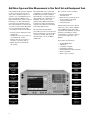
PSA Series Spectrum Analyzers
Noise Figure Measurements Personality
Technical Overview with Self-Guided Demonstration
Option 219
The noise figure measurement
personality, available on the
Agilent PSA Series spectrum
analyzers, provides a suite
of noise figure and gain
measurements including
system calibration.
Add Noise Figure and Gain Measurements to Your Set of Test and Development Tools
A key measurement in the development
of devices and systems is its noise
figure. The overall noise figure of a
system is one of the limiting factors
in its performance. Making noise
figure measurements can be a tedious
manual process. But with Agilent’s
noise figure measurement systems,
these measurements can be fast and
easy with accurate results. Meet many
of your measurement needs with
a one-analyzer solution from Agilent.
• Perform system calibration easily
and quickly.
• Analyze the device noise figure in
several different formats.
• Characterize the noise figure of
frequency conversion devices.
• Easily calculate measurement
uncertainty.
The noise figure measurements
personality provides noise figure and
gain measurements over the frequency range of the PSA with specified
measurements over the 10 MHz to
3 GHz range.
The technical overview includes:
• measurement details
• demonstrations
• PSA Series key specifications for
the noise figure personality
• ordering information
• related literature
All demonstrations use the Agilent
346C noise source, mixer, amplifier
and 70 MHz band pass filter. The
keystrokes surrounded by [] indicate
hard keys and while key names
surrounded by {} indicate soft keys
located on the right edge of the
display.
Noise figure measurements:
•
•
•
•
•
•
•
entering ENR values
calibration
noise figure and gain
using display features
measurement uncertainty calculator
mixer as the DUT
mixer as part of system
Demonstration
preparation
page 3
Scale and
reference level
page 8
Noise figure
summary
page 3
Markers
page 9
ENR table
noise source
page 4
Calibration
of noise figure
page 5
Noise figure
and gain
page 5
2
The Agilent PSA Series offers high
performance spectrum analysis up to
50 GHz with powerful one-button
measurements, a versatile feature set,
and a leading-edge combination of
flexibility, speed, accuracy and
dynamic range. Expand the PSA to
include noise figure measurements
with the noise figure measurements
personality (Option 219).
Format
change
page 9
Limit lines
page 10
Uncertainty
calculator
page 11
Display features
page 6
Mixer as
DUT
page 12
General, marker
and source tabs
page 7
Mixer as
system part
page 13
Demonstration preparation
To perform the following demonstrations,
the PSA requires these options.
Product type
Model number
Required options
PSA Series spectrum analyzer
E4440A/43A/45A/46A/48A Option 1DS built-in preamplifier
Option 219 noise figure measurement
personality
To configure the measurement
system, simply connect the noise
source (Agilent 346C) to the rear
panel connector labeled “noise source
drive out + 28 V (pulsed)” using a
1 meter BNC cable (50 Ω).
Noise figure measurement
process summary
Measuring the noise figure of a
device requires knowledge of the
measurement system. Once the noise
figure of the measurement instrument
is known and the gain of the device
under test (DUT) is known, then the
noise figure of DUT can be
calculated, after which the overall
noise figure is measured. Most
computing measurement systems,
such as the Option 219 measurement
personality, can display noise figure
in dB. Noise figure measurements
are comprised of three steps:
1. Enter the excess noise ratio ENR
values in dB of the noise source.
2. Calibrate the measurement
personality.
3. Make noise figure measurements.
3
Entering the ENR table
for a noise source
The noise source used for this
demonstration is the 346C. This
noise source has a calibrated range
of 10 MHz to 26.5 GHz. There is a
pulsed 28 V source that drives the
noise source. When the voltage is on,
the output of the noise source is the
excess noise value. Once calibration
data is entered into the measurement
personality, system calibration and
DUT measurements can be made.
In most cases a common ENR table
can be used for calibration and
measurements. However, in the case
of mixers, for example, the frequency
range of the source for measurements
may be outside the range for
calibration, and therefore two
sources are required. There are
instances where the calibration
ENR table is different from the
measurement ENR table. An example
would be the analysis of the noise
figure of a frequency conversion
device (mixer). In this case there is
no longer a common table used.
Instead, the common table function
is turned off. There are two methods
of loading the ENR information into
the table. The preferred method is to
load the values from a disk supplied
with the noise source. The second
method, which is less desirable, is to
enter the excess noise ratio common
table manually.
This exercise illustrates the different
methods of entering excess noise ratio
numbers.
4
Instructions
Keystrokes
Enable the noise figure measurement personality.
[Preset] [Mode] ({More} if necessary) {Noise
Figure}
Enter the ENR numbers from disk.
[File] {Load} {Type} {More}
{ENR Meas/Common Table} {Load Now}
You may also enter ENR values manually. Add
excess noise ratio (ENR) serial number and
model number.
{Meas Setup} {ENR} {Meas & Cal Table}
[Return] {Serial #}
Use the numeric pad and alpha editor to enter
the serial number. If the serial number already
exists, you will be prompted to choose whether
or not you want to load the data. If not, press
{Model ID} and enter the model number using
the alpha editor and numeric key pad.
Adding ENR values versus frequency.
{Index} [1] {Frequency} [10] {MHz}
{ENR Value} [13.14] {dB}
Repeat the process for index 2 and so on.
Saving the calibration data to a floppy or the
internal memory of the PSA.
[File] {Save} {Dir Select}
Use up/down arrows to select drive A for the
floppy, then press {Dir Select}. Press {Name}
and use the Alpha Editor to name the file
(8 characters max). When finished entering the
name, press [Return] and {Save Now}.
Calibration of the noise figure
measurement personality
In order to make accurate measurements, the personality must first be
calibrated. Calibration is required
because the NF of the measurement
system has to be known before a DUT
can be measured. The measured
instrument noise figure is then
removed from the total noise figure
measurement so that only the DUT
noise figure and gain is displayed.
Following is the calibration process:
1. Select the frequency range.
2. Set the number of points and set
the number of averages.
3. If the device under test does not
have gain or if the gain is low,
turn on the built-in preamplifier
before calibration.
Instructions
Keystrokes
Connect the noise source to the PSA with a
BNC cable to the source driver on the rear panel.
Connect BNC cable between 346 series
noise source and the rear panel connector
labeled Noise Source Drive Out +28 V (Pulsed).
Set the start frequency.
[Frequency] {Start Freq} [10] {MHz}
Set the stop frequency.
{Stop Freq} [3] {GHz}
Set the number of points at which to measure.
{Points} [30] [Enter]
Set the averaging function to 15 averages.
[Meas Setup] {Avg Number On} [15] [enter]
Calibrate the measurement personality.
[Meas Setup] {Calibrate} {Calibrate}
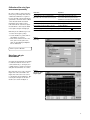
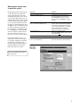
Figure 1.
DUT set up
Perform a system calibration.
Noise figure and gain
measurements
Now that the measurement personality
is calibrated with the noise source
connected directly to the input, it is
a simple matter to make noise figure
and gain measurements on a device.
Disconnect the noise source from the
input and connect the DUT to the
input and connect the noise source
to the DUT as shown in Figure 1. The
noise figure and gain of the device
under test is shown in Figure 2.
Figure 2.
Typical noise figure
and gain graph
5
Using the display features
The noise figure measurement
personality has many features to
help you interpret and analyze noise
figure measurements.
Select and Zoom Active Window:
This feature allows you to highlight
a window and then enlarge it for
closer analysis.
This exercise illustrates the use of the
display features.
Instructions
Keystrokes
Highlight the window of interest.
Press [Next Window] until the window
you want is highlighted.
Enlarge the window for closer analysis.
[Zoom]
Switch to another window (Figures 3 and 4).
[Next Window]
Figure 3.
Noise figure
full screen
Figure 4.
Device gain
full screen
6
General, markers
and source tabs
There are three tabs available at the
bottom of the screen. These tabs are
accessed using the left and right
arrow keys. The General tab shows
information about BW, number of
points, Tcold value, loss, attenuator
setting and internal preamplifier
setting. The Marker tab gives the
frequency, noise figure and gain of
each of the markers. The Source tab
includes information about the noise
source including serial number and
model identification.
Instructions
Keystrokes
View the tabs at the bottom of display
(Figures 5, 6, and 7).
Use the Right and Left Tab keys at the bottom
of the front panel to scroll through the tabs.
Figure 5.
General
information display
Figure 6.
Noise source
information
Figure 7.
Marker information
7
Scale and reference
level values
The scale in dB per division and
the reference values can be adjusted
to give an optimized view of the
measured results. The scale per
division can be adjusted in 0.1 dB
steps from 0 to 20 dB. The reference
level can be placed at the top of the
graph, in the center or at the bottom.
The reference level is adjustable
in 0.1 dB steps from –100 dB to
+100 dB.
Use the Auto Scale feature to give
the broadest view of the measured
trace. The lowest point will be placed
at the bottom of the graph and the
highest value at the top of the graph.
Perform display scaling.
8
Instructions
Keystrokes
Set the scale of the graphical view.
Press [Amplitude] [Next Window] to highlight
the graph to be changed. Press {Scale/Div}
and enter the new value [1.5] and press {dB}.
Set the reference value and the position
of the reference.
Press [Amplitude], then [Next Window] to
highlight the graph to be changed.
Press {Ref Value} and enter [18] and press {dB}.
Move the position of the Ref Value by pressing
{Ref Position Ctr}.
Expand the trace to fit the graph for a better
view of the measurement using the Auto Scale
function as shown in Figure 8.
Press [Amplitude] use [Next Window] to
highlight the graph to be expanded then press
{Auto Scale}.
Figure 8.
Display of noise
figure after
auto-scaling
Markers
A total of four normal markers can
be placed on the graphical display.
The placement of the markers is
limited to the calibration points.
If there are 11 calibration points
then the markers can be placed on
each of the vertical graticule lines.
Each of the normal markers can
be changed to delta markers. For
example, marker 2 will change to
marker 2 and 2R where 2R is the
reference and 2 would be the delta.
This exercise illustrates the use of
markers.
Change format of the active
window
The default view of the window is
the graphical mode with noise figure
in the top and gain in the bottom.
The two graphs can be combined to
display both traces on one graph.
There are two other views available
table mode and meter mode.
Instructions
Keystrokes
The marker function operates the same as
the standard E4440A series PSA.
To turn marker on, press [Marker].
Turn on marker 2.
Active delta marker 2.
Press {Select Marker 2} and press {Normal}.
First place the marker to a reference point
using knob or up/down arrows. Press {Delta}.
The marker table under the graphical display
reflects the delta marker information (Figure 9).
Move the marker relative to the reference
marker.
Switch between displaying the absolute
frequency of the delta marker and the
reference marker frequency.
Press {Delta Pair}. Note the change in
frequency above the graphical display.
Figure 9.
Display of markers
and delta markers
Instructions
Keystrokes
To combine both traces on one graph,
see Figure 10.
[Trace/View] {Combined on}
Activate the table mode.
[Trace/View] {Table}
Activate the meter mode.
[Trace/View] {Meter}
Figure 10.
Full screen of the
combined mode
Illustrating more of the display features.
9
Creating limit lines
Up to four limit lines can be set, two
for the upper graph and two for the
lower graph. The limit lines for the
upper graph are designated with up
arrows, and the limit lines for the
lower graph are designated with
down arrows. The limit lines can be
designated as upper limit or lower
limit and each can have a test
pass/fail indicator.
Instructions
Keystrokes
Open the limit line editor. Select upper limit for
the upper graph and turn on the limit test.
[Display] {Limits} {Limit Line 1} {Edit...}
Use right/left tab keys under display to highlight
“Limit”. Press {On}, tab to Type, press {Upper},
Display {On}, Test {On}.
Insert limit values for 10 MHz, 1, 2 and 3 GHz
(Figure 11).
Use right/left tab keys to highlight point 1.
{Frequency} [10] {MHz} {Limit Value} [5] {dB}
{Connected Yes} {Point 2} {Enter}
{Frequency} [1] {GHz} {Limit Value} [6] {dB}
{Connected Yes} {Point 3} {Frequency} [2] {GHz}
{Limit Value} [6.5] {dB} {Connected Yes}
{Point 4} {Frequency} [3] {GHz}
{Limit Value} [7] {dB} {Connected Yes}
This exercise develops limit lines.
Figure 11.
Display of limit line
10
Noise figure uncertainty
calculator
When making a noise figure measurement, there are many aspects of the
measurement setup that can affect
the uncertainty of that measurement.
The instrument uncertainty is one
element of measurement uncertainty
where the instrument itself adds to
the measurement uncertainty; this is
the instrument uncertainty we read
in the specifications. Other factors
like the noise source and the system
mismatch also add to the measurement uncertainty. A measurement
uncertainty calculator is used to
incorporate all of these factors to
determine the total measurement
uncertainty.
The noise figure measurement personality, Option 219, has a built-in
uncertainty calculator. To calculate
the overall measurement uncertainty,
simply choose the default noise source
(346C for example), enter the input
and output match of the device under
test and the gain/noise figure of the
DUT from the measurement display
and the value of the uncertainty will
be calculated. There are some default
values for the instrument (PSA)
already entered.
Instructions
Keystrokes
Select uncertainty calculator.
Choose 346C as default source.
[Mode Setup] {Uncertainty Calculator}.
Use right/left tab keys to highlight “Noise
Source Model” box. Press {346C}.
Enter the noise figure and gain values from
the measurements graph or marker table.
Use tab keys to highlight “DUT Noise Figure”
and enter [3.2] {dB}. (To view the marker table,
press [Return] and to return to the calculator
press {Uncertainty Calculator}). Then highlight
“DUT Gain” and enter [25] {dB}.
The input and output match of the DUT is
determined from the specifications sheet
or measured using a network analyzer.
Highlight “DUT Input Match” and enter [1.5].
Highlight “DUT Output Match” and enter [1.5].
The measurement uncertainty is then calculated
and the results is display at the bottom of the
form (Figure 12).
Figure 12.
Uncertainty
calculator display
Use the built-in uncertainty calculator.
11
Noise figure measurements
using a mixer as the DUT
When a down conversion is included
in the noise figure measurement, for
example measuring the noise figure
of a mixer, there are some additional
setups to consider. For this example
let us use a mixer as a down-converter
with an IF at 70MHz, LO at 1GHZ
and both RF sidebands are used,
930 and 1070 MHz (DSB):
• The measurement, as well as
calibration, is made at the
IF frequency.
• When an IF frequency is chosen,
it is a good idea to keep the
frequency as low as possible in
order to avoid large differences in
ENR values between the upper
and lower sidebands when using
DSB mode. This is because it is
the ENR value at the LO that is
used in the measurement
(compromise since it is centered
between the two sidebands)
• Since this device has some loss, it
is recommended that the internal
preamp be used.
• Compensate for two sidebands by
selecting double side band. Any
broadband noise in the LO will
directly affect results. This can
be solved by either a high pass or
low pass filter at the LO port that
removes the noise at the IF
frequency. Place an IF filter at the
input of the spectrum analyzer to
remove LO feed through. Usually
mixers have around 20 dB of
isolation between the LO-IF port
so the high powered LO will
seriously affect results.
Perform measurements on mixers.
12
Instructions
Keystrokes
Set up the PSA for down conversion
measurements. It is recommended that the
internal preamp be used when measuring
devices that have low gain.
{Meas Setup} {Int Preamp On}
[Mode Setup] {DUT Setup…} {Down Conv}
Set up the source for +7 dBm at 1 GHz.
On E4438C press [Frequency] [1] {GHz}
[Amplitude] [7] {dBm} [RF On].
Set up the LO frequency (Figure 13).
Scroll to “Ext LO frequency” using tab keys
then enter [1] {GHz}. Tab to “sideband” and
choose “DBS”.
Set up the fixed IF frequency.
[Frequency] {Freq Mode} {Fixed}
{Fixed Frequency} [70] {MHz}
Calibration: connect the noise source to
the input of the PSA.
[Meas Setup] {Calibrate} {Calibrate}
Measure the DUT: Connect the mixer IF (I)
port to the PSA, the LO (L) port to the signal
source and the RF (R) to the noise source.
To add more averaging, press [Meas Setup]
then {Avg Number On).
Figure 13.
Setup for
measuring a mixer
Measurements using a mixer
as part of the system
In this application the mixer is part
of the noise figure measurement
system. The diagram below shows
the DUT and the mixer as the down
converter. The DUT in this case is an
amplifier. When using a mixer as part
of the measurement system, calibration is performed with the mixer in
the path. As in the illustration above,
70 MHz is used as the IF and a band
pass filter is added to the IF out of
the mixer. Choose the LO frequency
to be 70 MHz above the desired RF
and then calibrate and then insert
the device under test. In this case,
the device is tested at one frequency.
In this measurement, there is no
input filter to limit the noise input
to the upper sideband even though
the LSB was selected. The noise
from the upper sideband and lower
sideband will give a noise figure
higher than expected (3 dB).
Instructions
Keystrokes
Setup for the calibration process.
Connect the noise source to the R port of
the mixer, the signal source to the L port
and the 70 MHz BPF to the I port. Connect
the other end of the 70 MHz BPF to the input
of the SA.
Analyzer setup - this assumes that the ENR
factors are loaded in the PSA (Figure 14).
[Mode Setup] {DUT Setup} {Amplifier}
Using the tab keys under the display, highlight
system downconverter and press {On}, move to
“LO” and enter [1] {GHz}. Move to “Sideband”
and select {LBS}. Move to “Frequency
Representation” and select “RF DUT Input”.
Set up the SA frequency.
[Frequency] {Freq Mode} {Fixed}
{Fixed Freq 930 MHz}. Set the source to 1 GHz
and +7 dBm. [RF On]
Start the calibration process.
[Meas Setup] {Calibrate} {Calibrate}
Place the DUT in the system between the
noise source and the RF port.
No key presses required; the noise figure and
gain is indicated in the box below the display.
Figure 14.
Setup using a
mixer as part
of the system
Perform measurements with a mixer as
part of the system.
13
PSA Series
Key Specifications
Noise figure measurement personality (200 kHz to 26.5 GHz)
Noise figure
Frequency range 200 kHz to 10 MHz
ENR
4 to 7 dB
12 to 17 dB
20 to 30 dB
(With internal preamp 1DS)
Meas. range
Instr. uncertainty
(nominal)
(nominal)
0 to 20 dB
±0.05 dB
0 to 30 dB
±0.05 dB
0 to 35 dB
±0.10 dB
Frequency range 10 MHz to 3 GHz
ENR
4 to 7dB
12 to 17 dB
20 to 22 dB
(With internal preamp 1DS and 1 MHz RBW)
Meas. range
Instr. uncertainty
0 to 20 dB
±0.05 dB
0 to 30 dB
±0.05 dB
0 to 35 dB
±0.10 dB
Frequency range 3 GHz to 26.5 GHz1
(With RBW of 1 MHz)
Measurement uncertainty
±0.3 dB (nominal)
ENR ~ 15 dB
Gain
Frequency range 200 kHz to 10 MHz
ENR
4 to 7 dB
12 to 17 dB
20 to 30 dB
(With internal preamp 1DS)
Meas. range
Instr. uncertainty
(nominal)
(nominal)
–20 to 40 dB
±0.17 dB
–20 to 40 dB
±0.17 dB
–20 to 40 dB
±0.17 dB
Frequency range 10 MHz to 3 GHz
ENR
4 to 7dB
12 to 17 dB
20 to 22 dB
(With internal preamp 1DS and 1 MHz RBW)
Meas. range
Instr. uncertainty
–20 to 40 dB
±0.17 dB
–20 to 40 dB
±0.17 dB
–20 to 40 dB
±0.17 dB
Frequency range 3 GHz to 26.5 GHz
(With RBW of 1 MHz)
Measurement uncertainty
±1.0 dB (nominal)
ENR ~ 15 dB
1. Performance above 3 GHz depends on the gain of
the DUT and whether or not a preamplifier is used.
Please refer to the Noise Figure Guide, literature
number E4440-90195, for details.
14
PSA Series Ordering
Information
PSA Series spectrum analyzer
E4443A
E4445A
E4440A
E4446A
E4448A
3 Hz to 6.7 GHz
3 Hz to 13.2 GHz
3 Hz to 26.5 GHz
3 Hz to 44 GHz
3 Hz to 50 GHz
Options
To add options to a product, use the following ordering scheme:
Model
E444xA (x = 0, 3, 5, 6 or 8)
Example options:E4440A-B7J or E4448A-1DS
Measurement personalities
E444xA-226
E444xA-219
E444xA-BAF
E444xA-210
E444xA-202
E444xA-B78
E444xA-214
E444xA-204
E444xA-211
E444xA-BAC
E444xA-BAE
E444xA-266
Phase noise
Noise figure
W-CDMA
HSDPA
GSM w/EDGE
cdma2000
1xEV-DV
1xEV-DO
TD-SCDMA
cdmaOne
NADC, PCD
HP 8566/8568B code compatibility
Requires Option 1DS
Requires Option B7J
Requires Options B7J and BAF
Requires Option B7J
Requires Option B7J
Requires Options B7J and B78
Requires Option B7J
Requires Option B7J
Requires Option B7J
Requires Option B7J
100 kHz to 3 GHz built-in preamplifier
Digital demodulation hardware
External mixing
Replaces type-N input connector
with APC 3.5 connector
70 MHz IF output
Available on E4440A/46A/48A only
Available on E4440A only
Hardware
E444xA-1DS
E444xA-B7J
E444xA-AYZ
E4440A-BAB
E444xA-H70
Connectivity software
E444xA-230
BenchLink Web Remote Control Software
Accessories
E444xA-1CM
E444xA-1CN
E444xA-1CP
E444xA-1CR
E444xA-045
E444xA-0B1
Rack mount kit
Front handle kit
Rack mount with handles
Rack slide kit
Millimeter wave accessory kit
Extra manual set including CD ROM
Warranty & Service
For warranty and service of 5 years, please order 60 months of R-51B (quantity = 60).
Standard warranty is 36 months.
R-51B
Return-to-Agilent warranty and service plan
Calibration1
For 3 years, order 36 months of the appropriate calibration plan shown below.
For 5 years, specify 60 months.
R-50C-001
Standard calibration
R-50C-002
Standards compliant calibration
E444xA-0BW Service manual and calibration software
E444xA-UK6 Commercial calibration certificate with test data
1. Options not available in all countries.
15
Product Literature
Selecting the Right Signal Analyzer
for Your Needs, selection guide,
literature number 5968-3413E
PSA Series literature
PSA Series, brochure,
literature number 5980-1283E
PSA Series, data sheet,
literature number 5980-1284E
NFA Series literature
NFA Series Configuration Guide,
literature number 5980–0163E
NFA, brochure,
literature number 5980–0166E
NFA Series Demonstration guide,
literature number 5980–2028E
Application literature
10 Hints for Making Successful
Noise Figure Measurements,
application note 1341,
literature number 5980–0288E
Fundamentals of RF and Microwave
Noise Figure Measurements,
application note 57-1,
literature number 5952–8255E
Noise Figure Measurement Accuracy
– The Y Factor Method,
application note 57-2,
literature number 5952–3706E
For more information on the
PSA Series, please visit:
www.agilent.com/find/psa
Agilent Technologies’ Test and Measurement
Support, Services, and Assistance
Agilent Technologies aims to maximize the value you
receive, while minimizing your risk and problems.
We strive to ensure that you get the test and
measurement capabilities you paid for and obtain
the support you need. Our extensive support
resources and services can help you choose the
right Agilent products for your applications and
apply them successfully. Every instrument and
system we sell has a global warranty. Support is
available for at least five years beyond the production
life of the product. Two concepts underlie Agilent’s
overall support policy: “Our Promise” and “Your
Advantage.”
Our Promise
Our Promise means your Agilent test and
measurement equipment will meet its advertised
performance and functionality. When you are choosing
new equipment, we will help you with product
information, including realistic performance
specifications and practical recommendations
from experienced test engineers. When you use
Agilent equipment, we can verify that it works
properly, help with product operation, and provide
basic measurement assistance for the use of
specified capabilities, at no extra cost upon request.
Many self-help tools are available.
Your Advantage
Your Advantage means that Agilent offers a wide
range of additional expert test and measurement
services, which you can purchase according to
your unique technical and business needs. Solve
problems efficiently and gain a competitive edge
by contracting with us for calibration, extra-cost
upgrades, out-of-warranty repairs, and onsite
education and training, as well as design, system
integration, project management, and other
professional engineering services. Experienced
Agilent engineers and technicians worldwide can
help you maximize your productivity, optimize the
return on investment of your Agilent instruments and
systems, and obtain dependable measurement
accuracy for the life of those products.
Agilent Email Updates
www.agilent.com/find/emailupdates
Get the latest information on the products and
applications you select.
Agilent T&M Software and Connectivity
Agilent’s Test and Measurement software and
connectivity products, solutions and developer
network allows you to take time out of connecting
your instruments to your computer with tools
based on PC standards, so you can focus on
your tasks, not on your connections. Visit
www.agilent.com/find/connectivity
for more information.
By internet, phone, or fax, get assistance with all your
test & measurement needs
Phone or Fax
United States:
(tel) 800 452 4844
Canada:
(tel) 877 894 4414
(fax) 905 282 6495
China:
(tel) 800 810 0189
(fax) 800 820 2816
Europe:
(tel) (31 20) 547 2323
(fax) (31 20) 547 2390
Japan:
(tel) (81) 426 56 7832
(fax) (81) 426 56 7840
Korea:
(tel) (82 2) 2004 5004
(fax) (82 2) 2004 5115
Latin America:
(tel) (305) 269 7500
(fax) (305) 269 7599
Taiwan:
(tel) 0800 047 866
(fax) 0800 286 331
Other Asia Pacific Countries:
(tel) (65) 6375 8100
(fax) (65) 6836 0252
Email: [email protected]
Online Assistance:
www.agilent.com/find/assist
Product specifications and descriptions in this
document subject to change without notice.
© Agilent Technologies, Inc., 2002, 2003
Printed in U.S.A., October 20, 2003
5988-7884EN