Download Precision Power A200.2 User`s guide

E-Prime
USER'S GUIDE
Walter Schneider*, Amy Eschman and Anthony Zuccolotto
Psychology Software Tools, Inc.
*Learning Research and Development Center, University of Pittsburgh
With assistance from:
Sara Burgess, Brandon Cernicky, Debbie Gilkey, Jennifer Gliptis,
Valerie Maciejczyk, Brian MacWhinney, Kimberly Rodgers, and James St. James
Copyright 2002 Psychology Software Tools, Inc.
All rights reserved.
Preface
The goal of developing the E-Prime suite of applications is to provide a common, standardized,
precise, computer research language for psychology that can be used on today's technologically
advanced computers. The E-Prime suite is designed to allow rapid development of experiments
that can be run with precision on computers around the world. A common computer language
enables researchers in different universities to communicate and share experimental procedures
and data. The system must be flexible enough to allow most psychological research that can be
run on computers to be implemented. It must also provide precision for accurate data analysis,
and even more important, internal auditing to enable the researcher to report the true precision of
the experiment. It is beneficial for the research community to have a dedicated staff of experts
interpreting and harnessing the rapidly changing computer environments to allow precision
experimentation on standard, commercial machines. The E-Prime suite was designed to be able
to be learned rapidly given the constraints of precision and flexibility of experimental procedures.
E-Prime is designed to match the way an experienced investigator structures and organizes an
experimental paradigm. There are now thousands of investigators that use E-Prime for research
on a daily basis to more effectively do high quality computer based experimental research.
Walter Schneider
Pittsburgh, PA, USA
Acknowledgements
The development of E-Prime has involved over twenty person years of effort. Many people have
contributed to the effort that has involved designing, running and testing nearly a million lines of
code. The initial design team included Walter Schneider, Anthony Zuccolotto and Brandon
Cernicky of Psychology Software Tools, Inc. and Jonathan Cohen, Brian MacWhinney and
Jefferson Provost, creators of PsyScope. The lead project manager was Anthony Zuccolotto
until the last year, when Brandon Cernicky assumed that role. The lead programmer and
manager of the project was Brandon Cernicky, who was in charge of all aspects of the Version
1.0 software development effort. Specific project programmers include Anthony Zuccolotto (ERun); Caroline Pierce (E-Merge, E-DataAid, E-Recovery); Jefferson Provost (E-Run and internal
factor architecture). The documentation management effort was led by Amy Eschman and
Valerie Maciejczyk. James St. James, Brian MacWhinney, Anthony Zuccolotto, and Walter
Schneider provided editorial assistance and drafted sections of the manual. Copy editing was
headed by Amy Eschman and Valerie Maciejczyk, assisted by Debbie Gilkey, Sara Burgess,
Kimberly Rodgers, Jennifer Gliptis, and Gary Caldwell. Version 1.0 testing involved Brandon
Cernicky, Anthony Zuccolotto, Amy Eschman, Debbie Gilkey, Sara Burgess, Jennifer Gliptis, and
Gary Caldwell. Sample experiments and Help files were created by Debbie Gilkey, Kimberly
Rodgers, Amy Eschman, Sara Burgess, and Brandon Cernicky. During the lengthy Beta
Program, Amy Eschman, Debbie Gilkey, Sara Burgess, Brandon Cernicky, and Anthony
Zuccolotto provided technical consulting and dealt with thousands of beta reports. Government
grant support in the form of SBIR grants from the National Science Foundation (Grant #III9261416 and DMI-9405202) and the National Institutes of Health (Grant #1R43 MH5819-01A1
and 2R44mh56819-02) covered significant research on code infrastructure, timing, and precision
testing. Partial support came from grants provided by the Office of Naval Research (Grant
#N0014-96C-0110) and the National Institutes of Health- NIMH (Grant #1R43 MH58504-01 and
2R44 MH58504-02) for research on biological extensions to the system.
Reference to E-Prime in Scientific Publications
It is important to describe the tools used to collect data in scientific reports. We request you cite
this book in your methods section to inform investigators regarding the technical specifications of
E-Prime when used in your research.
Schneider, W., Eschman, A., & Zuccolotto, A. (2002) E-Prime User’s Guide. Pittsburgh:
Psychology Software Tools Inc.
Schneider, W., Eschman, A., & Zuccolotto, A. (2002) E-Prime Reference Guide. Pittsburgh:
Psychology Software Tools Inc.
E-Prime User’s Guide
Table of Contents
Table of Contents
Chapter 1 : Introduction________________________________________________________________ 1
1.1
E-Prime_____________________________________________________________________ 1
1.2
Installation Instructions _______________________________________________________ 1
1.2.1
Machine Requirements for Intel PCs ___________________________________________ 1
1.2.2
Installing ________________________________________________________________ 1
1.3
Installation Options ___________________________________________________________ 2
1.3.1
Full Installation ___________________________________________________________ 2
1.3.2
Subject Station Installation __________________________________________________ 2
1.3.3
Custom Installation ________________________________________________________ 2
1.3.4
Run-Time Only Installation (Run-Time Only CD) ________________________________ 3
1.4
Hardware Key _______________________________________________________________ 3
1.4.1
Single User / Multi-Pack License _____________________________________________ 4
1.4.2
Site License ______________________________________________________________ 4
1.5
What to Know Before Reading This Manual ______________________________________ 4
1.6
Useful Information____________________________________________________________ 4
1.6.1
How to abort an experiment early _____________________________________________ 4
1.6.2
What to do if the hardware key fails ___________________________________________ 4
1.6.3
Locating the serial number___________________________________________________ 4
1.6.4
Sharing pre-developed programs ______________________________________________ 5
1.6.5
Citing E-Prime ____________________________________________________________ 5
1.7
E-Prime for MEL Professional Users_____________________________________________ 5
1.8
E-Prime for PsyScope Users ____________________________________________________ 8
Chapter 2 : Using E-Studio ____________________________________________________________ 11
2.1
Getting Started______________________________________________________________ 11
2.1.1
Design the experiment in stages______________________________________________ 11
2.2
Stage 1: Conceptualize and Implement the Core Experimental Procedure ____________ 12
2.2.1
Step 1.1: Provide an operational specification of the base experiment ________________ 12
2.2.2
Step 1.2: Create a folder for the experiment and load E-Studio _____________________ 13
2.2.3
Step 1.3: Specify the core experimental design _________________________________ 13
2.2.4
Step 1.4: Specify the core experimental procedure_______________________________ 13
2.2.5
Step 1.5: Set the non-default and varying properties of the trial events _______________ 14
2.2.6
Step 1.6: Specify what data will be logged for analysis ___________________________ 16
2.2.7
Step 1.7: Run and verify the core experiment___________________________________ 17
2.2.8
Step 1.8: Verify the data logging of the core experiment __________________________ 18
2.3
Performing Stage 1: Implement the Core Experimental Procedure __________________ 18
2.3.1
Perform Step 1.1: Provide an operational specification of the base experiment _________ 19
2.3.2
Perform Step 1.2: Create a folder for the experiment and load E-Studio ______________ 19
2.3.3
Perform Step 1.3: Specify the core experimental design __________________________ 21
2.3.4
Perform Step 1.4: Specify the core experimental procedure________________________ 22
2.3.5
Perform Step 1.5: Set the non-default and varying properties of the trial events ________ 23
2.3.6
Perform Step 1.6: Specify what data will be logged for analysis ____________________ 24
2.3.7
Perform Step 1.7: Run and verify the core experiment ____________________________ 25
2.3.8
Perform Step 1.8: Verify the data logging of the core experiment ___________________ 27
Page i
E-Prime User’s Guide
Table of Contents
2.4
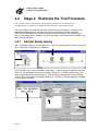
Stage 2: Elaborate the Trial Procedure _________________________________________
2.4.1
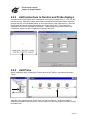
Add Get Ready display ____________________________________________________
2.4.2
Add instructions to Fixation and Probe displays_________________________________
2.4.3
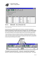
Add Prime______________________________________________________________
2.4.4
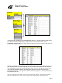
Add Feedback ___________________________________________________________
2.4.5
Run and verify the Get Ready, Prime, and Feedback objects _______________________
30
30
31
31
33
34
2.5
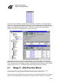
Stage 3: Add All Conditions, Set Number of Trials and Sampling ___________________
2.5.1
Add all conditions________________________________________________________
2.5.2
Set the weights __________________________________________________________
2.5.3
Set the sampling mode and exit condition _____________________________________
2.5.4
Test ___________________________________________________________________
34
34
38
38
40
2.6
Stage 4: Add Block Conditions ________________________________________________
2.6.1
Add a block List object____________________________________________________
2.6.2
Move the DesignList to BlockProc___________________________________________
2.6.3
Add block instructions ____________________________________________________
2.6.4
Add Introduction and Goodbye to SessionProc _________________________________
2.6.5
Modify TrialProc to use PrimeDuration _______________________________________
2.6.6
Special notes: Multiple methods to divide a design between levels __________________
40
40
41
42
42
43
44
2.7
Stage 5: Add Practice Block __________________________________________________
2.7.1
Duplicate BlockList in the Browser __________________________________________
2.7.2
Add block level attribute PracticeMode _______________________________________
2.7.3
Use script to terminate practice based on accuracy ______________________________
49
50
50
51
2.8
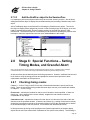
Stage 6: Special Functions – Setting Timing Modes, and Graceful Abort _____________ 53
2.8.1
Checking timing modes ___________________________________________________ 53
2.8.2
Providing early graceful abort of a block ______________________________________ 54
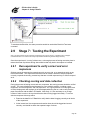
2.9
Stage 7: Testing the Experiment_______________________________________________
2.9.1
Run experiment to verify correct and error responses ____________________________
2.9.2
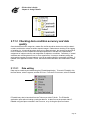
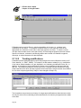
Checking scoring and data collection _________________________________________
2.9.3
Checking timing accuracy _________________________________________________
2.9.4
Running pilot subjects ____________________________________________________
55
55
55
56
56
2.10 Stage 8: Running the Experiment _____________________________________________ 57
2.10.1
Running subjects_________________________________________________________ 57
2.10.2
Running on multiple machines ______________________________________________ 58
2.11 Stage 9: Basic Data Analysis __________________________________________________
2.11.1
Merging data____________________________________________________________
2.11.2
Checking data condition accuracy and data quality ______________________________
2.11.3
Analysis and export of data_________________________________________________
59
59
61
63
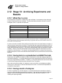
2.12 Stage 10: Archiving Experiments and Results ___________________________________
2.12.1
What files to store ________________________________________________________
2.12.2
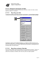
Saving data in a spreadsheet and EDAT formats ________________________________
2.12.3
Saving results of analyses __________________________________________________
67
67
67
67
2.13 Stage 11: Research Program Development ______________________________________
2.13.1
Modifying experiments____________________________________________________
2.13.2
Sending experiments to colleagues___________________________________________
2.13.3
Developing functional libraries______________________________________________
68
68
68
69
Chapter 3 : Critical timing in E-Prime - Theory and recommendations _________________________ 71
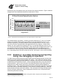
3.1
Page ii
Executive Summary of E-Prime Timing Precision and Implementation Methods _______ 71
E-Prime User’s Guide
Table of Contents
3.2
Introduction to Timing Issues__________________________________________________ 72
3.2.1
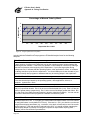
Problem 1: Computer operating systems can falsely report timing data_______________ 75
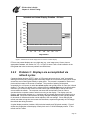
3.2.2
Problem 2: Actual durations can deviate from intended durations ___________________ 76
3.2.3
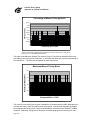
Problem 3: Displays are accomplished via refresh cycles__________________________ 79
3.2.4
Problem 4: Accurately measuring and reporting timing, then debugging an experiment __ 83
3.3
Achieving Accurate Timing in E-Prime__________________________________________ 84
3.3.1
Basic timing techniques and implementations in E-Prime__________________________ 84
3.4
Implementing Time Critical Experiments in E-Prime ______________________________ 96
3.4.1
Step 1. Test and tune the experimental computer for research timing _________________ 97
3.4.2
Step 2. Select and implement a paradigm timing model ___________________________ 97
3.4.3
Step 3. Cache stimulus files being loaded from disk to minimize read times __________ 120
3.4.4
Step 4. Test and check the timing data of the paradigm___________________________ 120
Chapter 4 : Using E-Basic ____________________________________________________________ 123
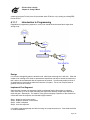
4.1
Why Use E-Basic? __________________________________________________________ 123
4.1.1
Before Beginning… ______________________________________________________ 124
4.1.2
Basic Steps_____________________________________________________________ 126
4.2
Introducing E-Basic _________________________________________________________ 126
4.2.1
Syntax ________________________________________________________________ 127
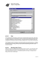
4.2.2
Getting Help____________________________________________________________ 128
4.2.3
Handling Errors in the Script _______________________________________________ 130
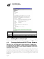
4.3
Communicating with E-Prime Objects _________________________________________ 130
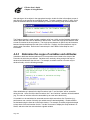
4.3.1
Context________________________________________________________________ 131
4.3.2
Object.Properties ________________________________________________________ 132
4.3.3
Object.Methods _________________________________________________________ 132
4.3.4
Variable Declaration and Initialization _______________________________________ 133
4.3.5
User Script Window vs. InLine Object _______________________________________ 134
4.4
Basic Steps for Writing E-Prime Script _________________________________________ 135
4.4.1
Determine the purpose and placement of the script ______________________________ 135
4.4.2
Create an InLine object and enter the script____________________________________ 135
4.4.3
Determine the scope of variables and attributes_________________________________ 136
4.4.4
Set or reference values in script _____________________________________________ 138
4.4.5
Reference script results from other objects ____________________________________ 139
4.4.6
Debug_________________________________________________________________ 140
4.4.7
Test __________________________________________________________________ 142
4.5
Programming: Basic ________________________________________________________ 142
4.5.1
Logical Operators________________________________________________________ 142
4.5.2
Flow Control ___________________________________________________________ 142
4.5.3
Examples and Exercises___________________________________________________ 148
4.5.4
Additional Information ___________________________________________________ 153
4.6
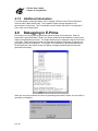
Programming: Intermediate __________________________________________________ 153
4.6.1
More on Variables _______________________________________________________ 153
4.6.2
Writing Subroutines ______________________________________________________ 155
4.6.3
Writing Functions _______________________________________________________ 156
4.6.4
Additional Information ___________________________________________________ 157
4.7
Programming: Advanced ____________________________________________________ 157
4.7.1
Arrays ________________________________________________________________ 157
4.7.2
Timing ________________________________________________________________ 160
4.7.3
User-Defined Data Types__________________________________________________ 160
Page iii
E-Prime User’s Guide
Table of Contents
4.7.4
4.7.5
Examples _____________________________________________________________ 160
Additional Information ___________________________________________________ 162
4.8
Debugging in E-Prime ______________________________________________________ 162
4.8.1
Tips to help make debugging easier _________________________________________ 164
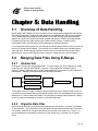
Chapter 5 : Data Handling ___________________________________________________________ 165
5.1
Overview of Data Handling __________________________________________________ 165
5.2
Merging Data Files Using E-Merge____________________________________________
5.2.1
Introduction____________________________________________________________
5.2.2
Organize Data Files _____________________________________________________
5.2.3
Merge ________________________________________________________________
5.2.4
Conflicts ______________________________________________________________
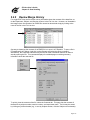
5.2.5
Review Merge History ___________________________________________________
165
165
165
166
173
177
5.3
Data Handling Using E-DataAid ______________________________________________
5.3.1
Introduction____________________________________________________________
5.3.2
Reduce the Data Set _____________________________________________________
5.3.3
Understand the Audit Trail ________________________________________________
5.3.4
Edit Data ______________________________________________________________
5.3.5
Analysis ______________________________________________________________
5.3.6
Use the Results _________________________________________________________
5.3.7
Secure Data____________________________________________________________
5.3.8
Export Data____________________________________________________________
5.3.9
Import Data____________________________________________________________
179
179
179
186
188
191
199
203
206
206
References ________________________________________________________________________ 207
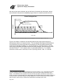
Appendix A: Timing Test Results ______________________________________________________ A-1
Running the RefreshClockTest _____________________________________________________ A-2
Meaning of Individual Results______________________________________________________ A-5
E-Prime Timing Tests____________________________________________________________ A-11
Test Equipment Details __________________________________________________________ A-13
Appendix B: Considerations in Computerized Research ___________________________________ A-19
Experimental Design Considerations _______________________________________________ A-19
Definitions _____________________________________________________________________ A-19
Dependent and Independent Variables ______________________________________________ A-19
Controls _____________________________________________________________________ A-20
Before Beginning … _____________________________________________________________
What are the questions that need to be answered? _____________________________________
How can the research questions be answered? ________________________________________
How will data be analyzed? ______________________________________________________
How will the experimental tasks be presented? _______________________________________
A-21
A-21
A-21
A-22
A-22
Implementing a Computerized Experiment __________________________________________
Constructing the experiment______________________________________________________
Pilot testing___________________________________________________________________
Formal data collection __________________________________________________________
Familiarizing subjects with the situation ____________________________________________
Where will data collection take place? ______________________________________________
Is a keyboard the right input device? _______________________________________________
A-22
A-22
A-23
A-23
A-24
A-24
A-25
Page iv
E-Prime User’s Guide
Table of Contents
The Single-Trial, Reaction-Time Paradigm __________________________________________ A-25
General Considerations___________________________________________________________ A-26
An example experiment __________________________________________________________ A-26
What happens on each trial? ______________________________________________________ A-26
What happens within a block of trials? ______________________________________________ A-28
Blocked versus random presentation ________________________________________________ A-28
Ordering of trials within a block ___________________________________________________ A-29
What happens within the whole experiment? _________________________________________ A-29
Instructions ___________________________________________________________________ A-30
Practice ______________________________________________________________________ A-30
Debriefing ____________________________________________________________________ A-30
How many trials? ________________________________________________________________ A-31
Between- Versus Within-Subjects Designs ___________________________________________ A-31
Other Considerations in RT Research _______________________________________________ A-32
Speed-accuracy trade-off _________________________________________________________ A-32
Stimulus-response compatibility ___________________________________________________ A-33
Probability of a stimulus _________________________________________________________ A-33
Number of different responses_____________________________________________________ A-33
Intensity and contrast ____________________________________________________________ A-34
Stimulus location _______________________________________________________________ A-34
Statistical Analysis of RT Data _____________________________________________________ A-35
Appendix C: Sample Experiments _____________________________________________________ A-37
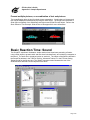
Basic Reaction Time: Text ________________________________________________________ A-37
Basic Reaction Time: Pictures _____________________________________________________ A-41
Basic Reaction Time: Sound _______________________________________________________ A-43
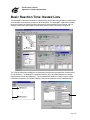
Basic Reaction Time: Nested Lists __________________________________________________ A-45
Basic Reaction Time: Extended Input _______________________________________________ A-46
Basic Reaction Time: Slide ________________________________________________________ A-48
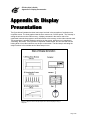
Appendix D: Display Presentation _____________________________________________________ A-53
Step 1 - Writing to Video Memory __________________________________________________ A-54
Step 2 - Scanning the Screen _______________________________________________________ A-54
Step 3 - Activating the Retina ______________________________________________________ A-55
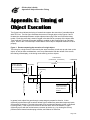
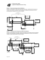
Appendix E: Timing of Object Execution _______________________________________________ A-57
Glossary__________________________________________________________________________ A-59
Page v
E-Prime User’s Guide
Chapter 1: Introduction
Chapter 1: Introduction
1.1
E-Prime
E-Prime is a comprehensive suite of applications offering audited millisecond-timing precision,
enabling researchers to develop a wide variety of paradigms that can be implemented with
randomized or fixed presentation of text, pictures and sounds. E-Prime allows the researcher to
implement experiments in a fraction of the time required by previous products, or by programming
from scratch. As a starting point, the Getting Started Guide provides much of the knowledge to
implement and analyze such experiments. Upon completion of the Getting Started Guide, the
User’s Guide will provide further understanding of the components included within E-Prime.
1.2
Installation Instructions
Please review all of the information in this section before installing the system.
1.2.1
Machine Requirements for Intel PCs
The full E-Prime installation requires approximately 100 MB disk space. A summary of the
machine requirements is listed below.
Minimum
•
•
•
•
•
Recommended
Windows 95
120 MHz Pentium Processor
16-32 MB RAM
Hard Drive (100 MB free for full install)
15” SVGA Monitor and Graphics Card
with DirectX™ compatible driver
support*
CD-ROM
•
*4 MB VRAM necessary for 1024x768 24-bit
color.
1.2.2
•
•
•
•
•
•
•
•
•
Windows 98/ME
Pentium III
64 MB RAM
Hard Drive (100 MB free for full install)
PCI/AGP Video Card with DirectXTM compatible driver
support and 8 MB+ VRAM
17-21” SVGA Monitor
PCI Sound Card with DirectXTM compatible driver
support and option for on-board memory
Network Adapter
CD-ROM
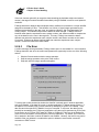
Installing
Installation of the E-Prime system requires the E-Prime CD (located in a CD sleeve inside the
Getting Started Guide cover) and hardware key (included in the shipment), as well as a valid
serial number (located on the CD sleeve).
Ø
Ø
Ø
Connect the hardware key to the parallel or USB port.
Close all Windows applications.
Place the E-Prime CD into the CD-ROM drive.
The installation program will launch automatically. Alternatively, the installation may be launched manually by
running the SETUP.EXE program from the CD-ROM drive, or by accessing the Add/Remove Programs option
in the control panel.
Ø
Select the type of installation to run and follow the instructions on the screen.
The default installation is recommended. This places E-Prime in the C:\ProgramFiles\PST\E-Prime…directory.
Descriptions of installation options may be found in section 1.3.
Ø
Restart the machine.
Page 1
E-Prime User’s Guide
Chapter 1: Introduction
1.3
Installation Options
1.3.1
Full Installation
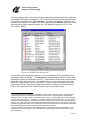
The full installation provides the entire suite of E-Prime applications. The table below lists the
applications included with the full installation.
Application
Use
Relevant File(s)
E-Studio
Examination or modification of
experiment specifications, generation of
EBS files
Stimulus presentation, Data collection,
Demonstration
Merging of data files
Experiment Specification (ES)
E-Basic Script (EBS), Data files
(EDAT)
Data Files (EDAT, EMRG)
Examination, Analysis, Export,
Regeneration of tables or analyses
Conversion of E-Run text files to EDAT
files.
Stimulus List creation.
Data Files (EDAT, EMRG)
Analysis Files (ANL)
Text data files (TXT) generated by ERun
Excel spreadsheets (XLS)
E-Run
E-Merge
E-DataAid
E-Recovery
Factor Table Wizard
1.3.2
Subject Station Installation
E-Prime must be installed locally in some manner on every machine on which its use is intended.
However, the entire E-Prime system does not need to be installed on machines used only for
collecting data or demonstrating pre-created programs. The E-Prime installation includes a
Subject Station install that is approximately half the size of the full installation, and permits the
running of pre-compiled E-Basic Script (EBS) files for demonstration or data collection. To install
the run-time application and only those components necessary for running pre-generated EBS
files, insert the E-Prime CD into the CD-ROM to launch the installation program. During
installation, choose the Subject Station option. Repeat the Subject Station installation on all data
collection machines.
The Subject Station installation supplies the E-Run application only. This option does not permit
the development of new programs, or the generation of EBS files from Experiment Specification
(ES) files. The E-Run application is not copy protected. Hence, the hardware key must be
connected only during installation. The Subject Station installation may be installed on multiple
machines in a lab in order to collect data from more than one subject at a time. Refer to the End
User License Agreement (EULA) for additional information regarding the use of the Subject
Station installation.
When using the Subject Station installation, it is recommended that the researcher run a program
to test that the installation was completed successfully prior to attempting to run actual subjects.
The BasicRT.EBS file is included with the Subject Station installation for this purpose
(C:\Program Files\PST\E-Prime\Program\BasicRT.EBS). To run any other EBS file using a
Subject Station machine, simply copy the EBS file to that machine, load the script into E-Run, and
click the Run button.
1.3.3
Custom Installation
The custom installation provides the ability to choose which applications will be included or
omitted during installation. Although used rarely, this installation option may be used to save
space on the computer’s hard drive. For example, if developing an experiment is the only utility
needed, then the E-Prime Development Environment is the best option. The E-Run option is
Page 2
E-Prime User’s Guide
Chapter 1: Introduction
equivalent to a Subject Station or Run-Time Only install, and the E-Prime Analysis and Data File
Utilities option is ideal for just merging and analyzing data.
During installation, the installation program will prompt the user for the specific applications to be
installed. Check all of the applications to be installed, and leave unwanted applications
unchecked. The Description field lists the components included with a selected option. The
amount of space required by an installation option, and the amount of space available on the
machine are displayed below the checklist.
1.3.4
Run-Time Only Installation (Run-Time Only CD)
A Run-Time Only installation option is available by separately purchasing the Run-Time Only CD.
This option is available for collecting data at a site other than where the full E-Prime system is
licensed. For example, a study may require data to be collected at a location other than where
the experiment is designed and analyzed (e.g., multi-site study). The Run-Time Only CD will
allow data collection by providing the E-Run application, but none of the other E-Prime
applications are installed.
The Run-Time Only CD is a separate compact disk from the complete E-Prime CD, and does not
require the hardware key for installation. However, before installing, all previous versions of the
E-Prime run-time installation must be un-installed. To do so, go to the computer’s Control Panel
via the “My Computer” icon and select the “Add/Remove Programs” icon. Then scroll down the
“Install/Uninstall” tab to highlight the necessary application(s), and click the Remove button.
To install the Run-Time Only CD, insert it into the CD-ROM Drive of the computer needed for
data collection. Refer to section 1.2.2 for further installation instructions.
1.4
Hardware Key
E-Prime is a copy-protected system requiring a hardware key that connects to the computer’s
parallel or USB port. The parallel port hardware key is a pass-through device, allowing a printer
to be connected to the machine as well. The hardware key copy protection scheme limits the
number of development machines to the number of licenses purchased. The hardware key is
required for installation of E-Prime. Other applications require the hardware key to be installed
depending on the type of license in use.
Page 3
E-Prime User’s Guide
Chapter 1: Introduction
1.4.1
Single User / Multi-Pack License
A single user license allows the user to develop experiments on one computer at a time. The
hardware key must be connected during installation of E-Prime, and while developing
experiments within E-Studio. E-Studio will not load if the hardware key is not connected.
However, the run-time application (E-Run) is not copy protected. E-Run may be installed on any
number of machines within a single lab, and used for data collection on multiple machines
simultaneously.
With the single user license, users may install E-Prime on multiple machines, and simply move
the hardware key to the machine to be used for experiment development. If more than one
development station is necessary, additional licenses must be purchased. When multiple single
user licenses are purchased (Multi-Pack License), each license is shipped with its own hardware
key.
1.4.2
Site License
A site license permits an unlimited number of E-Prime installs within the licensed department.
The site license requires the hardware key to be connected only during installation. The site
license does not require the hardware key for the use of E-Studio.
1.5
What to Know Before Reading This
Manual
Before reading this manual, a user should have a basic knowledge about operating personal
computers and experimental research design and analysis. A working knowledge of Windows is
essential, and at least one undergraduate course in experimental research methods is
recommended. The understanding of terms such as “independent variables” and “random
sampling” will be assumed. If this background is missing, it is recommended that the user first go
through a basic text describing how to use the Windows operating system and an undergraduate
text on experimental research methods. Furthermore, this text assumes the experience of
working through the Getting Started Guide accompanying the E-Prime CD.
1.6
Useful Information
1.6.1
How to abort an experiment early
Press Ctrl+Alt+Shift to terminate the E-Run application. A dialog box will appear confirming the
decision to abort the experiment. Click OK. The E-Run application will terminate. Within the EStudio application, an error dialog will appear displaying the “Experiment terminated by user”
message.
1.6.2
What to do if the hardware key fails
Users should not experience any problems installing or using E-Prime if the hardware key is
correctly in place, and the serial number was correctly entered. However, if the hardware key
should fail, contact PST immediately (see Technical Support below).
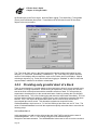
1.6.3
Locating the serial number
The serial number is located on the CD sleeve containing the E-Prime CD, inside the cover of the
Getting Started Guide. Place the serial number in an appropriate place so that it is readily
Page 4
E-Prime User’s Guide
Chapter 1: Introduction
accessible. Once E-Prime has been installed, the serial number can also be found in the About
E-Studio dialog box located on the Help menu. Users MUST provide the serial number for
technical support.
1.6.4
Sharing pre-developed programs
E-Prime license owners are free to distribute any files they create through use of the system.
Files created by users include Experiment Specification files (ES) , E-Basic Script files (EBS) ,
data files (EDAT, EMRG) , and analysis files (ANL) . However, the license agreement prohibits
distribution of any part of the E-Prime system, including the run-time application. Therefore, in
order to view or run any shared files, the recipient must have access to an E-Prime installation.
The E-Prime Evaluation Version may be used to view experiments and run them under restricted
conditions. To access an ES file, the recipient must have the full E-Prime installation, or a
custom installation including E-Studio. To run an EBS file, the recipient must have the Subject
Station installation, a custom installation including E-Run, or the Run-Time Only installation. To
open or merge data files, the user must have an installation including the data handling
applications (i.e., E-DataAid and E-Merge). For further information about sharing pre-developed
files, refer to the Reference Guide (Chapter 3, section 3.3.5).
1.6.5
Citing E-Prime
Technical details should be reported in the Methods sections of articles presenting experiments
conducted using E-Prime. The reader should consult the American Psychological Association's
Publication Manual (1994) for a general discussion of how to write a methods section. The EPrime User's Guide and Reference Guide may be referenced as follows:
Schneider, W., Eschman, A., & Zuccolotto, A. (2001). E-Prime User's Guide. Pittsburgh:
Psychology Software Tools, Inc.
Schneider, W., Eschman, A., & Zuccolotto, A. (2001). E-Prime Reference Guide. Pittsburgh:
Psychology Software Tools, Inc.
1.7
E-Prime for MEL Professional Users
MEL Professional users often ask how E-Prime differs from MEL Professional. Having invested a
large amount of effort to learn MEL Professional and the MEL language, users would like to be
assured that their investment will not be wasted. The following section will outline the differences
and similarities between MEL Professional and E-Prime. While MEL Professional users will find
that there are a number of similarities between the two systems, there are sufficient differences to
warrant a few recommendations. It is strongly recommended that even the most experienced
MEL Professional user work through the Getting Started Guide as an introduction to E-Prime.
Also, when recreating experiments originally written using MEL Professional in E-Prime, it is
recommended that the user not attempt to use any code from MEL Professional programs. MEL
language commands do not automatically convert to E-Basic script, and it is best that the user
attempt to remap the structure of the experiment in E-Prime from scratch. The amount of time
that was necessary to generate an experiment using MEL Professional has been greatly reduced
with E-Prime (e.g., hours instead of days).
At the most basic level, MEL Professional and E-Prime differ in the operating systems for which
they were designed. MEL Professional, released in 1990, was designed for achieving accurate
timing within the MS-DOS operating system. E-Prime was developed for use with Windows,
specifically responding to advancing technology, and the need for a more advanced tool
compatible with modern operating systems. MEL Professional users viewing E-Prime will notice
Page 5
E-Prime User’s Guide
Chapter 1: Introduction
a great difference in the appearance of the interfaces. By adhering to Windows standards, EPrime has a more familiar look and feel, and will ease the transition from one tool to the other. As
an analogy, MEL Professional can be contrasted with E-Prime in the same way that MS-DOS can
be contrasted with Windows. Windows accomplishes the same basic functions as those
available in MS-DOS, but does so using a graphical interface, with a great deal more ease and
flexibility. Though some of the concepts are the same when moving from MS-DOS to Windows,
one must think differently when working within the Windows interface. Likewise, when comparing
MEL Professional and E-Prime, the packages are similar in that they both allow the creation of
computerized experiments with high precision. However, E-Prime introduces a graphical
interface, and the user must learn to compose experiments using graphical elements, by dragging
and dropping objects to procedural timelines, and specifying properties specific to those objects.
E-Prime offers a more three-dimensional interface than that of MEL Professional. To view
settings within a MEL Professional experiment, the user was required to move through various
pages (i.e., FORMs), and examine the settings in the fields on each of those pages. The FORMs
were displayed in numerical order, but the numbering (supplied by the user) did not necessarily
offer any indication as to the relationships between FORMs or the order in which they were
executed (e.g., TRIAL Form #2 was not necessarily executed second). None of the settings were
applied to the FORMs themselves, and the program would have to be executed in order to see
effects such as a change in font color. Thus, it was difficult for the user to easily identify the
relationships between different events within the experiment (i.e., how FORMs related to each
other), and how specific settings would affect the display.
E-Prime offers a more WYSIWYG (What You See Is What You Get) type of interface, displaying
the hierarchical structure of the experiment and relationships between objects in one location.
There are various methods by which the user may view settings for an object defining a specific
event, and by opening an object in the workspace, the user can see an approximate
representation of what will be displayed during program execution.
The most notable difference between MEL Professional and E-Prime is a conceptual one. EBasic, the language underlying E-Prime, is an object-based language that encapsulates both data
and the methods used to manipulate that data into units called objects. MEL Professional used a
proprietary language, the MEL language, which was developed specifically for research purposes
and had no real relationship to existing procedural languages. E-Basic is a more standardized
language, with greater transferability of knowledge when scripting, and greater flexibility to allow
user-written subroutines. E-Basic is almost identical to Visual Basic for Applications, with
additional commands used to address the needs of empirical research. E-Basic is extensible to
allow an experienced programmer to write Windows DLLs to expand E-Prime’s functionality with
C/C++ code. In most cases, however, the need to insert user-written script and the amount of
script required is significantly decreased.
While the direct similarities between MEL Professional and E-Prime are few, users familiar with
MEL Professional and the design of computerized experiments will find that they are able to
transfer a great deal of knowledge when developing experiments using E-Prime. For example,
experience with the structure of experiments and the concept of levels (e.g., Session level, Block
level, etc.), as well as with the organization of data used within the experiment in INSERT
Categories is still very much a part of experiment creation using E-Prime. This experience is not
wasted when moving from MEL Professional to E-Prime, rather it permits the user to more quickly
develop an understanding of E-Prime. The concepts of experiment structure and data
organization remain the same, but the implementation of these concepts within E-Prime has been
greatly improved. In addition to the graphical representation of the hierarchical structure of
events within the experiment, the access of the data used in the experiment has been made
much easier. In E-Prime, data is referenced using the names of attributes in a List object rather
than by referring to an INSERT Category slot number (e.g., E-Prime allows the user to refer to the
Page 6
E-Prime User’s Guide
Chapter 1: Introduction
“Stimulus” attribute rather than {T1}). Other tasks involving the INSERT Category that are very
cumbersome in MEL Professional are made much easier by the List object in E-Prime, such as
sampling from more than one list on a single trial, sampling multiple times from the same list on a
single trial, and setting different randomization schemes for different sets of data.
To indicate the order of events and maintain timing precision, MEL Professional used the concept
of Event Lists and Event Tables. While quite powerful, Event Tables were difficult to understand,
and required variable locking, which restricted access to variable values until the Event Table
finished executing. E-Prime improves upon the Event List concept with the Procedure object,
which allows users to organize events in a more informative graphical interface, and PreRelease,
which allows the user more control over the setup time required by program statements.
Another similarity between MEL Professional and E-Prime is the range of applications offered to
the user. MEL Professional was a complete tool, offering development, data collection, merging
and analysis applications. Once again, E-Prime offers a variety of applications to provide
comparable functionality, and greatly improves upon the ease of use of these applications. For
example, MEL Professional offered the MERGE program to merge separate data files into a
master file for analysis. E-Prime offers the same functionality with the E-Merge application, but
improves the process by allowing the user to simply select the files to merge and click a single
button to complete the process. As with the development application, all applications within EPrime offer a Windows interface, making each more familiar, and easier to use and learn. The
run-time application, E-Run, provides the same time-auditing features that were available to the
MEL Professional user in order to verify the timing of events in the program. With E-Prime,
however, time-auditing occurs more easily, requiring the user only to turn on data logging for a
specific object. E-Prime simplifies data merging and analysis tasks as well, and removes some of
the restrictions enforced by MEL Professional (e.g, MEL Pro collected only integer data). With EPrime, all values are logged in the data file as strings, but the Analyze command is able to
interpret the appropriate variable type (e.g., integer, string, etc.) during analysis. In addition, EPrime affords compatibility between data files including different ranges for a single variable, or
variables added during different executions of the same program. Even data files collected by
completely different experiments may be merged.
The differences between MEL Professional and E-Prime are too numerous to itemize in this
section. However, based on years of product support for MEL Professional, certain differences
warrant special mention. A major emphasis during the development of E-Prime was concern for
the preservation of data, and data integrity. MEL Professional allowed data for multiple subjects
to be collected into a single data file, which could result in tremendous loss of data if the data file
became corrupted. To safeguard against data loss, E-Prime collects only single subject data
files, and offers the E-Recovery utility in the event that the data file is lost or corrupted. In
addition, the handling of data has been made much easier and more flexible. To accompany this
flexibility, each data file maintains a history of modifications, and security options may be set to
restrict access to certain variables, or to restrict operations on data files. Finally, MEL
Professional users often reported forgetting to log an important measure, and recreating the
randomization sequence to log that measure could be a difficult and lengthy process. To avoid
errors such as this, E-Prime uses the concept of “context”. All data organized in the List object
within E-Prime is automatically entered into the context, and all context variables are logged in
the data file unless logging is specifically disabled.
MEL Professional users will also be thrilled that they are no longer restricted by specific brands of
audio and video cards. While presentation of sounds and images using MEL Professional
depended upon a great deal of information (video card manufacturer, image resolution, color
depth, etc.), the presentation of sounds and images using E-Prime does not require the user to
know anything other than the name and location of the image (*.BMP) files to be presented, or
Page 7
E-Prime User’s Guide
Chapter 1: Introduction
the format of the WAV files (e.g., 11,025Hz, 8 Bit, Mono). Most video and audio cards offering
DirectX support are compatible with E-Prime. Other restrictions imposed by MEL Professional
are alleviated by E-Prime. Reaction times are no longer restricted to a maximum integer value of
32767ms, and experiments are no longer restricted to a maximum of three levels (i.e., Session,
Block, Trial). E-Prime allows for up to 10 levels in the experiment structure (e.g., Session, Block,
Trial, Sub-Trial, etc.), and users have the ability to rename experiment levels (e.g., Passage,
Paragraph, Sentence, etc.).
The goal of E-Prime is to simplify the process of computerized experiment generation, while
providing the power to perform tasks required by the research community. With a Windowsbased environment and an object-based language, E-Prime facilitates experiment generation for
programmers and non-programmers alike, while offering the most powerful and flexible tool
available.
1.8
E-Prime for PsyScope Users
- Contributed by Brian MacWhinney, Carnegie Mellon University
PsyScope users often ask how E-Prime differs from PsyScope. Having invested a large amount
of effort to learn Psyscope, users would like to minimize the effort needed to learn to use EPrime. The following section will outline the differences and similarities between PsyScope and
E-Prime. PsyScope users will find that there are a number of similarities between the two
systems.
In building E-Prime, we relied in many ways on the design of PsyScope. As a result, much of EPrime has a touch and feel that is reminiscent of PsyScope. For example, the E-Prime Procedure
object uses the timeline metaphor of the PsyScope Event Template window. Similarly, the EPrime List object looks much like a PsyScope List window. In designing E-Prime, we also tried to
preserve the ways in which PsyScope made the design of the experiment graphically clear. The
E-Prime Structure view expresses much of what the PsyScope interface expressed through
linked objects in the Design window. We also preserved much of PsyScope’s user interface in
terms of the general concepts of ports, events, and factors. For example, a PsyScope event and
an E-prime object are conceptually identical, since an event is an object in a graphic timeline for
the trial.
However, when one gets under the hood, the two products are entirely different. The most
obvious difference is that the current release of E-Prime runs only on Windows. For the
PsyScope user familiar with the Macintosh user interface, the idiosyncrasies of Windows can be
frustrating. It simply takes time to get used to new methods of handling the mouse, expanding
and contracting windows, and dragging objects.
The other major difference is that E-prime uses E-Basic as its underlying scripting language,
thereby fully replacing PsyScript. PsyScript was a powerful language, but users with little
programming background found it difficult to master some of its conventions. The documentation
for PsyScript was often incomplete or difficult to follow. E-Basic, like Visual Basic for Applications,
is extremely well documented and conceptually easier than PsyScript. More importantly, there
was a great potential in PsyScope to break the link between the graphical user interface (GUI)
and the script. In some cases, a script could not be edited again from the GUI after these links
were broken. E-Prime, on the other hand, allows the user to write small blocks of E-Basic script
for specific objects or actions. This means that the user can use the scripting language to make
targeted minor modifications without affecting the overall graphic interface.
Page 8
E-Prime User’s Guide
Chapter 1: Introduction
Because the two products are fundamentally different, it is strongly recommended that even the
most experienced PsyScope user work through the Getting Started Guide as an introduction to EPrime. PsyScope users who have spent a few hours working with Windows programs will quickly
realize that many aspects of the E-Prime interface are simply echoes of Windows metaphors.
This is particularly true for the system of window control, and navigation in E-Studio and the
Structure view. We designed these components using metaphors from Windows utilities such as
Windows Explorer, which are familiar to Windows users. For the Mac user, who is unfamiliar with
Windows, some of these approaches, such as manipulation of the Structure view, will seem
unnatural and clumsy. However, after a bit of exploration, they become easy to use.
The biggest improvement that E-Prime makes over PsyScope is in the way that it avoids deep
embedding of actions in the user interface. In PsyScope, it was often necessary to click down
three or four levels to link objects between the Factor Table and a stimulus list. In addition, the
properties of levels of the design as realized in the Factor Table were only accessible by going
through the template for each cell and then down to the individual lists. In E-Prime, the various
views allow greater access to properties (e.g., Workspace, Properties window, Attributes viewer),
and the highlighting of attribute references through color-coding visually indicates to the user
which properties are varying.
E-Prime’s second major advance over PsyScope, which we discussed earlier, is the fact that
users can embed blocks of E-Basic code virtually at will directly within the visual environment. In
PsyScope, one had to choose between using the graphic environment or using PsyScript. In EPrime, one can have scriptability within the graphic environment using E-Basic. E-Basic is an
object-based language that encapsulates both data and the methods used to manipulate that
data into units called objects. E-Basic is almost identical to Visual Basic for Applications, with
additional commands used to address the needs of empirical research. E-Basic is extensible to
allow an experienced programmer to write Windows DLLs to expand E-Prime’s functionality with
C/C++ code.
The third major advance in E-Prime is its stability. As users are well aware, PsyScope was prone
to bugs and crashes. Many of these problems were caused by complex interactions between the
windowing environment and the operating system. Typically, users would build up complex
designs in a factor table and then not be able to consistently apply local changes to particular
levels. Eventually, PsyScope would lose track of objects and the whole experiment would crash.
E-Prime has conquered these problems. However, one casualty of this clean-up has been
elimination of the flexible system of PsyScope windows, including the modal windows, the
expandable Factor Table, dynamic script updating, and the “ports” dialog for building screen
displays. These same facilities are available in E-Prime, but they are less dynamic. For
example, while the PsyScope script was active and displayed modifications immediately, E-Prime
is more of a graphical user interface, and requires the user to regenerate the script in order for
changes to be viewed. At the same time, the overall interface is much more stable and less
prone to crashing.
The fourth major advance in E-Prime is its significantly improved system of display and response
time measurement. Although timing was accurate in PsyScope, few tools were provided to the
user that would allow them to verify timing. E-Prime provides these tools along with careful
documentation on how to maximize precision and test for accuracy. Many of these tools are
automated. For example, one can turn on time audit variables in logging and the accuracy of
presentation will be continually recorded and stored in the data output file.
The fifth major advance in E-Prime is its tighter linkage to data output. In PsyScope, researchers
could use PsyDat, PsySquash, or their own scripts to control the movement of data to statistical
programs. E-Prime handles data movement and processing through the E-Merge and E-DataAid
Page 9
E-Prime User’s Guide
Chapter 1: Introduction
modules. These modules replace the methods of PsyDat and PsySquash with the more familiar
metaphor of the Excel spreadsheet. Users of PsyDat who also know Excel will simply give up
thinking about data analysis through PsyDat and switch to thinking in terms of Excel, as
implemented by E-Merge and E-DataAid. To safeguard against data loss, E-Prime collects only
single subject data files, and offers a recovery utility in the event that the data file is lost or
corrupted. Each data file maintains a history of modifications, and security options may be set to
restrict access to certain variables, or to restrict operations on data files.
These five features all make the transition from PsyScope to E-Prime relatively easy. Of course,
there are still new things to learn. One way of managing the transition from PsyScope to E-Prime
relies on examining specific scripts for identical experiments in the two systems. Users who wish
to use this method to transition to E-Prime can access comparable scripts by going to
http://psyscope.psy.cmu.edu for PsyScope scripts and http://step.psy.cmu.edu for E-Prime
scripts.
Page 10
E-Prime User’s Guide
Chapter 2: Using E-Studio
Chapter 2: Using E-Studio
This chapter describes the general methods of implementing an experiment in E-Prime. Note,
Appendix B-Considerations in Research provides an overview of experimental research concepts
without reference to E-Prime. This chapter assumes the user has worked through the concepts
of experimental design and the Getting Started Guides for each of the applications within EPrime. The user should, by now, have a basic understanding of E-Prime, and general knowledge
concerning working in a Windows application. This chapter is appropriate to read before
implementing the first experiment from scratch.
2.1
Getting Started
To program a good experiment, clearly conceptualize the experiment before implementing it in EStudio. Clearly state what variables are to be manipulated, what the experimental procedures
are, what data will be collected, and how the data will be analyzed (“how to” explanations of the
preceding items are to follow in this chapter). Conceptualizing the experiment will save time and
create better research. Too many times, an experiment is run and data collected before the
analysis is fully visualized.
2.1.1
Design the experiment in stages
There is an enormous amount of detail in any experiment. It is often best to design the
experiment in a series of stages, each containing a few steps. This substantially speeds
development and reduces errors. It is best to design a stage, then implement and test that stage
before implementing the next stage. Experiencing a few trials helps to conceptualize and plan
the other segments of the experiment. The recommended stages of implementing an experiment
are:
Conceptualize and implement the core experimental procedure
Elaborate the Trial procedure
Add all the trial conditions to the experiment
Add blocks and block conditions
Set sampling frequency, selection method, and number of samples
Add special functions – cumulative timing, practice blocks
Test the experiment
Run the experiment
Perform basic data analysis
Archive experiments and results
Research program development – modify experiments, send experiments to colleagues, develop
libraries
We will go through each of the stages sequentially. We recommend designing and implementing
an experiment in stages. Note, it might be good to try to answer most of the design questions
(see Stage 1 below) before implementing the experiment. Whether the design is done before
implementing the experiment or as the experiment is being implemented, we recommend actually
performing the implementation in stages.
Page 11
E-Prime User’s Guide
Chapter 2: Using E-Studio
2.2
Stage 1: Conceptualize and Implement
the Core Experimental Procedure
The goal of this stage is to get the basic procedure implemented to the point where the
experiment presents at least two different instances of the trial procedure. Be clear on the trial
procedure and what data are to be collected. We will first give an overview of the steps and then
give specific instructions for performing the steps. We present the graphical objects from E-Prime
to help associate the experimental specification with the visual interface in E-Prime.
We recommend reading through the next few pages to conceptualize the relationship of the
experimental steps and the E-Prime implementation without trying to do it on the computer.
First conceptualize how to go from an experimental idea to a computer exercise. Then we will go
back over the steps and show how to implement each stage. Note, in this text, we will include
images from E-Prime to show the relationship between experimental concepts and the E-Prime
objects and interface. Wait until this chapter’s section on Performing Stage 1 (section 2.3) to
actually implement the experiment.
Stage 1: Conceptualize and implement the core experimental procedure
Provide an operational specification of the base procedure
Create a folder for the experiment and load E-Studio
Specify the core experimental design, independent variables, stimuli, and expected responses
Specify the core experimental procedure
Set the non-default and varying properties of the Trial events
Specify what data will be logged for analysis
Run and verify the core experiment
Verify the data logging of the core experiment
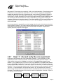
2.2.1
Step 1.1: Provide an operational specification of
the base experiment
Operationally identify the experiment that you are trying to develop. What is being manipulated?
What is the expected outcome? State clearly the expected effect the independent variables might
have on the dependent variables. For example, in a lexical decision experiment, the
experimenter might present text strings that are either words or non-words, and record the
reaction time for the subject to categorize the stimulus as a word or a non-word. The question
might be whether it is faster to recognize a string of letters as a word or a non-word. It is useful to
write a draft of the abstract for the experiment being implemented, particularly detailing the
procedure. For the lexical decision experiment this might be:
The experiment will measure the time to make a lexical decision. The independent
variable is whether a letter string is a word or a non-word. The subject will be
presented with a fixation (+) displayed in the center of the screen for one second.
Then a probe display will present a letter string stimulus in the center of the screen
for up to 2 seconds. The stimulus display will terminate when the subject responds.
Subjects are to respond as quickly as possible as to whether the stimulus was a word
or a non-word by pressing the “1” or “2” key respectively. The dependent measures
are the response (i.e., key pressed), response time, and response accuracy of the
probe display. The stimuli will be words and non-words, presented in random order
in black text on a white background.
In Stage 1, we will implement the above procedure. In Stage 2, we will elaborate both the
description and the experiment.
Page 12
E-Prime User’s Guide
Chapter 2: Using E-Studio
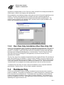
2.2.2
Step 1.2: Create a folder for the experiment and
load E-Studio
We recommend developing the experiments in the standard directory “My Experiments” on the
root directory. We suggest that the experiment be placed in a folder named for the experimental
series (e.g., C:\MyExperiments\LexicalDecision) and that the experiment name include a number
for the version of the experiment (e.g., LexicalDecision001).
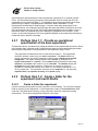
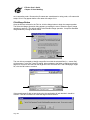
2.2.3
Step 1.3: Specify the core experimental design
Be able to specify the design of the experiment and list all of the conditions, stimuli, and expected
responses. The abstract of the lexical decision experiment includes the following details about
the design; The independent variable is whether a letter string is a word or a non-word… The
stimuli will be text strings of words and non-words… Subjects are to respond as quickly as
possible as to whether the stimulus was a word or a non-word by pressing the “1” or “2” keys
respectively. Note, the bolding in the abstract highlights key terms that will directly influence the
names or settings in the E-Prime experiment specification. The design of the lexical decision
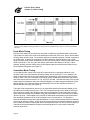
experiment can be implemented in a table, such as the following:
Condition
Stimulus
Correct Response
Word
NonWord
cat
jop
1
2
It is good to start out with the basic design, implement it and then elaborate on it. In this case, we
start with one independent variable (Condition) having two levels or cells (Word, Non-Word). For
each cell, the table contains a separate line. We need to specify the stimulus that determines
what the subject sees in that condition and the correct response to the stimulus, which
determines how the response is scored. Later, we can add more independent variables (e.g.,
word frequency and priming), stimuli, and associated responses.
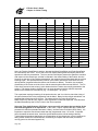
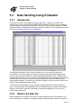
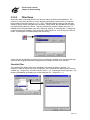
In E-Prime, the design is specified using List objects. For example, the specification above
would result in a List object with the following form:
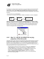
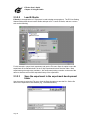
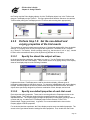
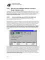
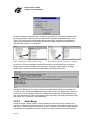
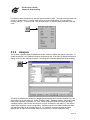
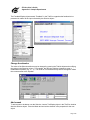
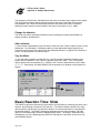
2.2.4
Step 1.4: Specify the core experimental
procedure
The core experimental procedure is a minimal, repetitive portion of an experiment in which
different conditions are selected, stimuli are presented, and the subject responds. The core
procedure typically defines the sequence of trials the subject experiences. It is useful to make a
diagram of the sequence of events. This involves two things: specifying the sequence of events
and connecting the design to the events.
Page 13
E-Prime User’s Guide
Chapter 2: Using E-Studio
For example, in the lexical decision experiment, the core experimental procedure was described
in the abstract: The subject will be presented with a fixation (+) displayed in the center of the
screen for one second. Then a probe display will present a letter string stimulus in the center of
the screen for up to 2 seconds. The lexical decision procedure can be specified in a list of events
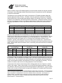
as follows:
- Select the stimulus from the DesignList
- Present the Trial Procedure which contains: Fixation, then Probe, and collect the response
Select
Stimulus
Fixation
Probe Display/
Collect Response
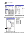
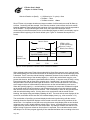
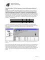
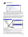
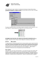
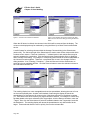
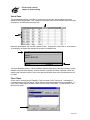
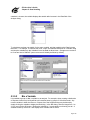
In E-Prime, the core structure of the experiment is specified through the combination of a List
object (e.g., DesignList) to select the conditions, a Procedure object (e.g., TrialProc) to specify
the sequence of events in a trial, and events specific to that procedure (e.g., Fixation and Probe
display). The E-Prime Structure view below shows the outline of the experimental procedure.
The structure shows the outline of the experiment with the core being the DesignList and the
TrialProc, including the Fixation and Probe events.
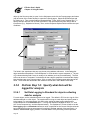
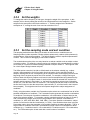
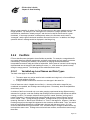
2.2.5
Step 1.5: Set the non-default and varying
properties of the trial events
The specific nature of each stimulus can be specialized by setting critical properties of the stimuli.
E-Prime provides defaults for dozens of properties for each stimulus (e.g., font style, forecolor,
background color, location, duration, etc.). The properties that do not have a default value must
be set (e.g., text in the fixation display to be a “+”), as must any properties that differ from the
default. Also the properties that vary in the experiment (e.g., based on the condition) must be set.
The abstract specified a series of properties that must be set:
The stimuli will be words and non-words, presented in random order in black text on
a white background. The subject will be presented with a fixation (+) displayed in
the center of the screen for one second. Then a probe display will present a letter
string stimulus in the center of the screen for up to 2 seconds. The stimulus
display will terminate when the subject responds. Subjects are to respond as
quickly as possible as to whether the stimulus was a word or a non-word by pressing
the “1” or “2” key respectively.
Page 14
E-Prime User’s Guide
Chapter 2: Using E-Studio
For the lexical decision experiment, the fixed and varying properties can be summarized in the
following table:
Object
Fixed Properties
Varying Properties
Fixation
•
•
•
•
•
•
•
•
•
•
•
•
Probe
Present “+” in the center of the screen
Duration = 1 second (default)
Forecolor = black (default)
Background color = white (default)
Display in center of the screen (default)
Duration = 2 seconds
Input keys = “1” and “2”
Terminate display upon response
Forecolor = black (default)
Background = white (default)
Stimulus (e.g., “cat”, “jop”, etc.)
Correct response = “1” or “2”
Fixed display text. For the fixation stimulus, specifying the fixed text “+” for the fixation is a
must. This is done by typing the “+” in the text area of the Fixation TextDisplay object.
Varying display text. For the Probe stimulus, the text varies from trial to trial. To specify a
varying property, create an attribute in a List object, assign values to the levels (i.e., rows) of that
attribute, and then refer to the attribute in other objects. In this case, the text string is specified in
the Stimulus attribute (column) of the DesignList. To reference the attribute, enter the attribute
name enclosed in square brackets [ ] . Entering [Stimulus] refers to the attribute Stimulus that
can be assigned multiple values (e.g., “cat” or “jop”). The Stimulus attribute (i.e., [Stimulus]) is
entered into the Text field of the Probe object to present different strings across trials. On a given
trial, a row is selected from the List object, the value of the Stimulus attribute is determined (e.g.,
“cat” or “jop”), and this value is substituted for [Stimulus] on the Probe object.
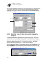
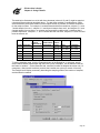
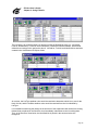
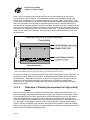
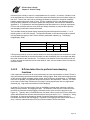
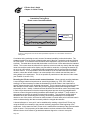
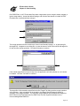
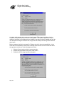
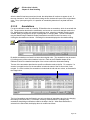
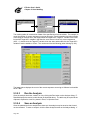
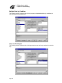
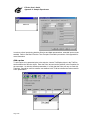
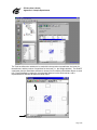
Non-default properties. In E-Prime, property settings are changed using fields on Property
pages. For the Probe display, the Duration/Input Property page is modified to set the Duration to
2000 in order to allow up to 2 seconds (2000 milliseconds) for the stimulus to be displayed. The
Page 15
E-Prime User’s Guide
Chapter 2: Using E-Studio
keyboard is designated as the Input Mask device, the allowed response keys (Allowable field) are
1 and 2, and the Correct field is set to refer to the CorrectResponse attribute (defined in the
DesignList). The End Action is set to the “Terminate” option to terminate the display when the
subject responds. These properties are set on the Duration/Input tab of the Probe TextDisplay
object (see arrows below).
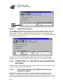
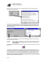
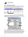
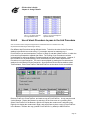
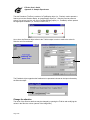
2.2.6
Step 1.6: Specify what data will be logged for
analysis
For a research experiment, the experimenter has to record and analyze data. This requires
clarity on what variables will be logged. Be able to answer, “What dependent measures will be
recorded in reference to specific objects in the experiment?” The abstract above stated: The
dependent measures are the response, response time, and response accuracy of the Probe
display. After a trial, expect to record the following information for the Probe display: What was
the response that the subject entered (i.e., 1 for word and 2 for nonword)? What was the
response time? What was the accuracy (i.e., 1 for correct and 0 for wrong)?
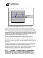
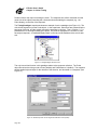
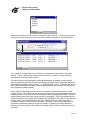
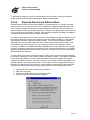
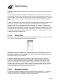
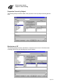
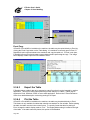
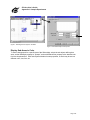
In E-Prime, each object is capable of logging multiple properties. Setting the data logging for an
object to “Standard” will result in the logging of the RESP (response), RT (reaction time) and
ACC (accuracy) properties (as well as other dependent and time audit measures). Data logging
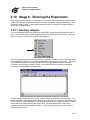
is set via the Duration/Input tab in the object’s Property pages.
Page 16
E-Prime User’s Guide
Chapter 2: Using E-Studio
Why doesn’t E-Prime simply log everything? Well it could, and technically, if Data Logging is set
to Standard on every object in the experiment, it would. However, logging everything greatly
expands the data that is stored in an experiment and, more seriously, increases the number of
variables to go through when analyzing an experiment. Note, if we logged every property of
every object in a typical experiment, this could require logging several hundred variables per trial.
The vast majority of these variables will never be examined (e.g., the response of hitting the
spacebar to advance the instruction display). The default settings in E-Prime log all of the design
variables (specified in List objects) and require the user to specify logging on all objects that
collect critical data.
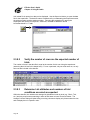
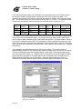
It is the experimenter’s responsibility to set the logging option for each critical object so the data
will be logged for analysis. This is done easily by setting the logging option for each object in the
experiment using the Duration/Input tab in the Property pages or using the Logging tab to
explicitly select the properties to be logged.
2.2.7
Step 1.7: Run and verify the core experiment
At this point, the minimalist core of the experiment is specified. It is a good idea to run the
experiment and see if it works as intended. Recall the experimental procedure abstract: The
subject will be presented with a fixation (+) displayed in the center of the screen for one
second. Then a probe display will present a letter string stimulus in the center of the screen
for up to 2 seconds. What should we expect the first two trials to look like? Be able to draw out
the displays the subject would see. In this case, expect to see two trials, with the first presenting
a fixation “+” for one second and then the word “cat” for 2 seconds or until a response is entered.
Then the “+” is presented again, and the second stimulus “jop” is displayed until a response.
When running the experiment, verify that the stimulus is immediately removed when a response
is entered. If no response is entered, the stimulus should be displayed for 2 seconds. Expect to
see displays like the following:
+
cat
+
jo p
Page 17
E-Prime User’s Guide
Chapter 2: Using E-Studio
Press the “1” or “2” key, the text string will disappear, and the experiment will go to the next trial.
Note, each experiment run begins by asking for the subject number and session number (not
shown in this example).
2.2.8
Step 1.8: Verify the data logging of the core
experiment
An experiment is only useful if the critical data are recorded for later analysis. Be clear about
what expectations to see as input data for the analysis. From the abstract:
The independent variable is whether a letter string is a word or non-word… The
dependent measures are the response (i.e., key pressed), response time, and
response accuracy of the probe display.
In this case, basically expect to see the two rows of the DesignList plus the dependent measures
(subject response, response time, and accuracy of the response) in the data file. Analyze the
data using E-DataAid. The trial described above might appear like the following:
Independent Variables (from DesignList)
Condition
Stimulus
CorrectResponse
Word
cat
1
NonWord
jop
2
Dependent Variables (from run)
Probe.RESP Probe.RT Probe.ACC
1
586
1
1
1224
0
For trial 1 of this run of the experiment, the independent variables (attributes of the DesignList)
were Condition=Word, Stimulus=Cat, and CorrectResponse=1. The dependent variables were
the response key (Probe.RESP=1), response time (Probe.RT=586), and response accuracy
(Probe.ACC=1, indicating a correct answer). For trial 2, the Condition=NonWord, Stimulus=Jop,
CorrectResponse=2, Probe.Resp=1 (which mismatches the expected response),
Probe.RT=1224, and Probe.ACC=0 (indicating an error). Note, the average of all the Probe.ACC
values will give the average accuracy (1 for correct, 0 for error).
Stage 1 Summary. In steps 1.1 through 1.7 we conceptualized, implemented, and verified the
data logging of the core experiment, limiting the design to two cells. It is important at this stage to
conceptualize each of the steps discussed, and to relate them to the experimental procedures.
Exercise: For experiment development, draw the figures expected to occur, as above. In
particular, specify the 1) abstract of the core experiment; 2) folder name for the experiment and
where to keep it; 3) DesignList of the conditions, stimuli, and correct responses; 4) core
experimental procedure including when stimuli are selected and the trial procedure, including a
sequence of displays and subject responses; 5) non-default properties of the trial events,
including the fixed and varying text displays and the properties for how to display the stimulus, its
duration and termination condition, and the correct response; 6) what dependent measures will
be logged for further analysis; 7) expected subject displays (i.e., draw them), when responses
are to be made, and if they clear the screen; and 8) independent and dependent variables that
are logged for the experiment.
2.3
Performing Stage 1: Implement the
Core Experimental Procedure
In this section we will go over the specifics of performing each of the Stage 1 operations. To
perform the Stage 1 operations, we recommend reading through each step below and actually
Page 18
E-Prime User’s Guide
Chapter 2: Using E-Studio
implementing the specified feature of the lexical decision experiment on a computer using EPrime. We recommend working through the Getting Started Guide for creating an E-Prime
experiment prior to performing Stage 1. A completed version of the experiment at each stage
described in this chapter is included with the installation (default installation is C:\My
Experiments\Tutorials\Using E-Studio Stages). However, rather than going directly to the
completed version, we recommend going through each step sequentially, reading how to do the
step, performing the step in E-Prime, and verifying that the displays look as intended. Note, in
the section above, we simplified some of the displays to highlight the core concepts. In this
section, we will walk through the full E-Prime graphical displays to show where the information is
located and how to perform each stage.
2.3.1
Perform Step 1.1: Provide an operational
specification of the base experiment
This was done above, and amounts to writing the abstract for the experimental procedure. Below
is the abstract again, with bold words, indicating those aspects of the experimental specification
that set specific properties for the specification of the experiment using E-Prime:
The experiment will measure the time to make a lexical decision. The independent
variable is whether a letter string is a word or non-word. The stimuli will be text
strings of words and non-words, presented in random order in black text on a white
background. The subject will be presented with a fixation (+) displayed in the
center of the screen for 1 second. Then a probe display will present a letter string
stimulus in the center of the screen for up to 2 seconds. The stimulus display will
terminate when the subject responds. Subjects are to respond as quickly as
possible as to whether the stimulus was a word or a non-word by pressing the “1” or
“2” key respectively. The dependent measures are the response (i.e., key pressed),
response time, and response accuracy of the probe display.
2.3.2
2.3.2.1
Perform Step 1.2: Create a folder for the
experiment and load E-Studio
Create a folder for experiment
A place to develop the experiment on the computer is now necessary. This involves creating a
folder or directory for the experiment. For this experiment, create a "Lexical Decision" folder
under the C:\My Experiments directory on the computer in which the experiment is being
implemented. This is done using Microsoft Explorer’s File menu.
Page 19
E-Prime User’s Guide
Chapter 2: Using E-Studio
2.3.2.2
Load E-Studio
E-Studio is the application in E-Prime that is used to design an experiment. The E-Prime Getting
Started Guide shows how to load E-Studio and open a file. Launch E-Studio, and see a screen
such as the following:
For this example, open a blank experiment and use the File menu Save As option to save the
experiment as LexicalDecision001 in the C:\My Experiments\Lexical Decision folder. Most
experiments go through many variations. We recommend putting a number on the end of the
name to allow the return of the sequential history of the experiment.
2.3.2.3
Save the experiment in the experiment development
folder
Use the mouse to select the File menu, then the Save As option to save the file. Set the file
name to the experiment name desired (e.g., LexicalDecision001).
Page 20
E-Prime User’s Guide
Chapter 2: Using E-Studio
2.3.3
2.3.3.1
Perform Step 1.3: Specify the core experimental
design
Create and name the List object
The independent variables, stimuli, and expected responses are generally specified on a List
object. Drag a List object from the Toolbox to the SessionProc timeline. Rename the List1
object to DesignList by clicking on List1, pressing the F2 key (to enter Edit mode) and typing in a
new name for the object. The Structure view appears as the following:
2.3.3.2
Add the attributes for the design
Recall from the abstract that we wanted to implement the following condition table:
Condition
Word
NonWord
Stimulus
cat
jop
Correct Response
1
2
To do so, first open the DesignList object (double click on it in the Structure view). Then, click
the Add Multiple Attributes button. Specify that there are 3 attributes to add. Double click each
column header to change the attribute names for Attribute1, Attribute2, and Attribute3 to
Condition, Stimulus and CorrectResponse respectively (Note, no spaces are permitted in the
attribute name).
2.3.3.3
Add the needed rows and fill in the attributes for the
experiment
Implement the simplest version that illustrates the varying aspects of the experiment. This will
require having 2 rows (for Word and Non-Word). Click the Add Level tool button to add one row.
Then fill in the values for the levels of the attributes. Enter the values of the Condition, Stimulus,
and CorrectResponse attributes for two trials as shown in the next figure.
Page 21
E-Prime User’s Guide
Chapter 2: Using E-Studio
2.3.3.4
Create the Procedure
The Procedure attribute specifies what procedure to run for the selected condition. In this case,
set it to TrialProc as shown in the figure below. After entering “TrialProc” in the Procedure
attribute column, E-Studio will indicate that TrialProc has not yet been created and will ask to
create TrialProc. Answer “yes” to this prompt. At the end of step 1.3, for the lexical decision task,
the List object should look like this:
In Stage 1, we will not modify the sampling settings, and will leave the List with the default
settings (one cycle of two samples with sequential selection). We will change this in Stage 3.
2.3.4
Perform Step 1.4: Specify the core experimental
procedure
Implementing the core experimental procedure involves specifying the trial events and setting the
fixed and varying properties of the trial objects.
2.3.4.1
Put the trial events on the TrialProc timeline and
rename the objects
Double click the TrialProc in the Structure view to open the trial procedure timeline in the
Workspace. To add displays to the Procedure, click an object from the display class (e.g.,
TextDisplay, ImageDisplay, SlideDisplay, SoundOut) and drag it to the TrialProc timeline. For our
lexical decision experiment, we need two TextDisplays for the Fixation and the Probe. To create
Page 22
E-Prime User’s Guide
Chapter 2: Using E-Studio
the Fixation and the Probe display objects, click the TextDisplay object icon in the Toolbox and
drag two TextDisplays to the TrialProc. The figure below shows both the Structure view and the
TrialProc after putting the TextDisplays on the TrialProc and renaming them appropriately.
2.3.5
Perform Step 1.5: Set the non-default and
varying properties of the trial events
The properties of each trial object/event must be set, if the desired settings differ from the default
settings. If a property does not vary throughout the experiment, it would be set to a constant
(e.g., the text “+” for fixation). When a property varies (e.g., the stimulus of “cat” or “jop”), it would
be set to refer to an attribute value (such as [Stimulus]) defined on a List object.
2.3.5.1
Specify the stimuli the subject will see
In the lexical decision experiment, the subject is to see a “+” for the Fixation and a value of the
Stimulus attribute for the Probe display. These values can be set by typing directly in the display
areas of the display objects as the following illustrates:
If objects other than a TextDisplay were used for the stimulus display, different types of
information might determine the basic stimulus. For example, ImageDisplays are used to display
bitmaps, SoundOut objects are used to present audio file output in WAV file format, and Slide
objects were specifically designed to present a combination of text, bitmaps, and sounds.
2.3.5.2
Specify non-default properties of each trial event
Each object has many properties. These can be set using either the Properties window or the
Property pages. The Properties window lists the properties related to a specific object in
alphabetical order. The Property pages arrange the properties in meaningful groupings under a
common tab (e.g., the tabs for the TextDisplay object include General, Frame, Font,
Duration/Input, Logging, and Notes). In general, it is recommended that the user use the
Property pages to set the properties.
For the lexical decision experiment, the Probe display requires some non-default properties. The
arrows in the figure below show the settings for these properties. First, double click the Probe
Page 23
E-Prime User’s Guide
Chapter 2: Using E-Studio
object (in the Structure view) to open it in the Workspace, and click the Property pages tool button
(top left corner of the Probe window) to open the Property pages. Select the Duration/Input tab
by clicking on it. Then, set the fields as illustrated below. Enter “2000” in the Duration field. To
specify the input devices, first click the Add button in the Input Masks list (lower left) to add an
input device (e.g., Keyboard or Mouse). Then, set the Response Options fields to define the input
conditions.
The fields in the experiment that vary may be set using attribute references. In the DesignList
object we defined the attribute “CorrectResponse” to code what the correct response is. The use
of [] indicates that the field Correct is usually a List attribute (such as [CorrectAnswer]). The End
Action can be set to Terminate if it is desirable for the subject's response to terminate the display.
Note that there are more Property pages. Click on each of the Property pages and examine the
fields. These fields are described in the Reference Guide and in the E-Basic Online Help.
2.3.6
2.3.6.1
Perform Step 1.6: Specify what data will be
logged for analysis
Set Data Logging to Standard for objects collecting
data for analysis
For each object, set the variables that are to be logged. The default in E-Prime is to log all of the
attributes defined on a List object. The experimenter must go to each object and specify what is
to be logged. For most experiments, this will involve setting the data logging option on the
Duration/Input tab to the Standard option. This logs the response variables of RESP, RT, and
ACC for the response key, and the response latency. For assistance, E-Prime will ask to set the
Data logging option to Standard whenever a value is specified for the Correct field (the rationale
being that specifying the correct answer will most likely facilitate analysis of the result later). In
addition, Standard data logging records Time Audit data to verify the timing of the experiment.
Page 24
E-Prime User’s Guide
Chapter 2: Using E-Studio
This includes the OnsetDelay and DurationError properties, which list timing data to check timing
precision (see Chapter 3 - Critical Timing).
2.3.6.2
Set specific logging as needed
On the Logging tab, set the logging to specific needs. Many of the properties of the object are
presented in a list, and are arranged in categories (Dependent Measures, Time Audit, etc.). It is
possible to select the properties independently by clicking the checkbox next to a specific
property, or as a group (click the first checkbox, then press the shift key down, click the last
checkbox of a group, and then click on one checkbox to set all of them). Properties for each
object are described in the Reference Guide as well as in the E-Basic OnLine Help.
2.3.7
2.3.7.1
Perform Step 1.7: Run and verify the core
experiment
Compile the experiment
At this point, the core experiment has been constructed, so it is time to test the experiment. Click
the Generate button to compile the experiment.
It is useful to view the results of the compile using the Output window in E-Studio. The Output
window may be displayed by choosing the Output option from the View menu. If no errors are
Page 25
E-Prime User’s Guide
Chapter 2: Using E-Studio
generated during the compiling process, a message indicating the successful generate is
displayed in the Output window.
If errors occur during generation, an error dialog is displayed, and the error message is sent to
the Debug tab in the Output window. The error message will indicate the line in the script at
which the error occurred. In addition, the Script window opens to display the line at which the
error was encountered.
Luckily, compile errors are rare. However, this same debugging technique can be used when
run-time errors are encountered.
2.3.7.2
Run trials responding correctly, incorrectly and not
responding
Run the experiment to test the core procedure. Click the Run button to launch E-Run and run the
experiment.
It is important to test the limits of an experiment to ensure that it behaves desirably, and that
scoring is occurring correctly. As the experiment is specified in the current example, the “1” and
“2” keys are the valid input keys, and the stimulus display is set to terminate upon valid input.
First, it is important to run “normal” trials, responding both correctly and incorrectly in order to
verify that the valid keys are being accepted as input and that the display is terminating upon
response. If the subject presses a valid response key during the 2000ms display, the display will
terminate and the next trial will be presented.
Page 26
E-Prime User’s Guide
Chapter 2: Using E-Studio
However, subjects don’t always follow the instructions, so it is necessary to test the deviant cases
as well. For example, what happens when a subject presses a key that is not a valid response
key, or perhaps does not respond at all? In the current example, pressing the wrong key or a
non-response will not terminate the display, but the stimulus display will terminate when the
maximum duration for the stimulus object is reached. If the subject presses an invalid key, or
does not respond within 2000ms, the experiment will simply continue with the next trial. At this
point, it is important to verify that this is how the trial procedure is working. Later, it will also be
necessary to verify the distinction between these trials (e.g., valid response versus invalid or nonresponse) through examination of the data file.
2.3.7.3
Verify expected displays
Verification of the core experiment also involves the examination of each of the displays. The
Fixation display presents a “+” for 1000ms. This display should be consistent in that the display
does not vary, nor does it terminate if the subject presses a key. However, the Stimulus display
should vary. The stimulus string presented should be different for each trial, and the duration of
the display is dependent upon the subject’s response (i.e., the stimulus is displayed until the
subject responds by pressing a valid key, or until the maximum duration of 2000ms has expired).
2.3.8
2.3.8.1
Perform Step 1.8: Verify the data logging of the
core experiment
Start E-DataAid and load the data
Once the core procedure has been verified, it is necessary to examine the data file in order to
determine that the information is logging correctly. The application that allows viewing and
editing of data files is E-DataAid. Open E-DataAid using the Tools menu in E-Studio. When EDataAid is launched, a screen such as the following will appear:
Page 27
E-Prime User’s Guide
Chapter 2: Using E-Studio
Until a data file is opened, no data can be displayed. Use the Open tool button, to open the data
file for the experiment. The data file name is determined by concatenating the Experiment name,
the subject number, and the session number. Following the suggestion for naming the
experiment and running as subject #1, session #1, the data file would be named
LexicalDecision001-1-1.edat.
2.3.8.2
Verify the number of rows are the expected number of
trials
The number of rows in the data file is equal to the number of trials run during the experiment
(assuming the trial level is the lowest level). For our experiment, only two trials were run, so only
two rows are included in the data file.
2.3.8.3
Determine List attributes and numbers of trial
conditions occurred as expected
Within the data file, the variables are arranged in alphabetical order by level (e.g., Block, Trial,
etc.) and may require some searching in order to find those columns of utmost interest. The
Arrange Columns dialog will allow hiding or moving columns to display only those wanted to view,
and to display them in a specific order.
Page 28
E-Prime User’s Guide
Chapter 2: Using E-Studio
.
Verify that the conditions, stimuli, and correct responses (i.e., independent variables) are logged
as expected.
2.3.8.4
Find the dependent variables and verify they are set
reasonably
Verify the logging of the dependent measures. The RESP property is the actual response
entered, and is logged as NULL for a non-response. The CRESP property is the correct answer,
which varies per trial, and ACC is the accuracy of the response (RESP) in relation to the correct
answer (CRESP). ACC is set to “1” for correct answers and to “0” for incorrect answers or
omissions. RT, of course, is the reaction time for the response measured from the onset of the
object collecting the input. Verify that the values logged for the dependent variables are as
expected for the test trials (e.g., RT values are appropriate for short and long response times, “0”
for omissions, etc.).
2.3.8.5
Check timing duration accuracy on fixed length
displays
Verifying timing precision is a critical function. Issues related to timing are detailed in Chapter 3 Critical Timing in the User's Guide. Here we will only provide brief accounts of timing issues. In
general, in E-Prime, the time from stimulus to response is accurately recorded. The duration from
stimulus to stimulus may be somewhat longer than specified in the Duration field. This is
because the display is written at the time of the vertical retrace (when the video monitor output of
the image goes to the top line of the display). The time from one display to the next is equal to
the duration of the first display plus the time until the next vertical blank interval. In this
experiment, the Fixation had a duration of 1000ms. The actual time from the Fixation to the
stimulus would be equal to the time of the duration of the Fixation plus the OnsetDelay of the
Probe object. It is important to verify this duration in order to accurately report the measured
fixation duration. In our experiment, use E-DataAid to examine the Probe.OnsetDelay variable
(should range from 0 to 17 milliseconds). To illustrate, if the Probe.OnsetDelay is 12, then the
fixation duration would be the duration (1000ms) plus 12ms, or 1012ms in length (see Chapter 3
– Critical Timing).
Page 29
E-Prime User’s Guide
Chapter 2: Using E-Studio
2.4
Stage 2: Elaborate the Trial Procedure
Note: This section builds on the experiment created during the previous section. A finished version of
LexicalDecision001.es is located in the C:\My Experiments\Tutorials\Using E-Studio Stages directory.
The goal of Stage 2 is to elaborate the basic Fixation-Probe trial procedure. A display will be
added at the beginning of the trial procedure to permit the subject to pace the trials and
instructions will be added to the Fixation display to remind the subject of the response keys.
Also, a Prime display will be added prior to the Probe display, and Feedback will be added to the
end of the trial procedure.
2.4.1
Add Get Ready display
Add a TextDisplay object as the first object in the TrialProc which allows the subject to set the trial
pace. Rename this TextDisplay to “GetReady.”
In the Text field, type “Press the spacebar when ready”. Allow the subject to begin the trial when
ready (i.e., set the duration to infinite by setting the duration to -1), enable keyboard input, and
enter the spacebar as the allowed input key. As a special key, the spacebar is entered as the
word "SPACE" (all capitals) surrounded by braces (i.e., {SPACE}). Set data logging to “standard”
to record subject wait time.
Page 30
E-Prime User’s Guide
Chapter 2: Using E-Studio
2.4.2
Add instructions to Fixation and Probe displays
Add instructions to the Fixation and Probe objects in the form of constant text (i.e., it will not vary
from trial to trial). Open the Fixation object, add four blank lines following the fixation character,
and type the text, as in the display below, to remind the subject of the response keys. Open the
Probe object and set the height of the display area (Frame tab) to 25%. This reduces the
displayed area to 25% in the center of the screen. These settings will permit the stimulus to
overwrite the fixation, but will not erase the response instructions.
2.4.3
Add Prime
Add a TextDisplay object following the Fixation object in the TrialProc, and rename this object
“Prime.”
Open the Prime object and type “[PrimeType]” into the Text field (i.e., the prime text will be
entered as an attribute value), as below. Set the duration for the Prime object to 1000ms, and do
not enable input.
Page 31
E-Prime User’s Guide
Chapter 2: Using E-Studio
Add an independent variable for coding PrimeType. Open the DesignList, add an attribute, and
name it PrimeType. Enter the values for PrimeType to be “word” and “non-word” as illustrated
below:
Finally, set the frame height for the Prime object to 25% so that the instructions from the Fixation
are not overwritten.
Page 32
E-Prime User’s Guide
Chapter 2: Using E-Studio
2.4.4
Add Feedback
Add a FeedbackDisplay object as the last event in the TrialProc, and rename it to Feedback.
Accept the standard feedback text settings for correct, incorrect, and non-responses. From the
dropdown box, select the Feedback object, and click the Properties tool button to set the
properties for the parent object. Set the Duration for the Feedback object to 2000ms.
Instruct the Feedback object to display feedback based on the scoring of the Probe object by
setting the Input Object Name (General tab in Feedback properties) to Probe. Accept the
standard statistics settings (collect ACC stats, No Response ACC Stats, RT Stats, and Incorrect
RT Stats) in order to collect reaction time and accuracy values, and log non-responses as
“Incorrect”.
Page 33
E-Prime User’s Guide
Chapter 2: Using E-Studio
2.4.5
Run and verify the Get Ready, Prime, and
Feedback objects
Save the experiment, compile it, and run it to verify that the new additions to the trial procedure
work as expected for all possible subject responses. Remember to test deviant as well as
expected cases (e.g., correct, incorrect, and invalid key responses).
2.5
Stage 3: Add All Conditions, Set
Number of Trials and Sampling
Note: This section builds on the experiment created during the previous section. A finished version of Stage2LexicalDecision001.es is located in the C:\My Experiments\Tutorials\Using E-Studio Stages directory.
The goal of stage 3 is to complete the DesignList object. This involves entering the complete
stimulus set, and setting the properties for the number of trials and the sampling method.
2.5.1
Add all conditions
We will be increasing the number of conditions, so the Condition attribute name no longer makes
a great deal of sense. Double click the header for the Condition attribute to rename it to
“ProbeType.” Rearrange the columns by clicking the column header to highlight the column, and
by clicking and dragging the header to a new location. A red line will appear as a visual cue for
where the column will be placed when the mouse button is released. Rearrange the columns as
follows:
Add exemplars (rows) to the DesignList to complete the listing of conditions and stimuli. Use one
of the three methods below to complete the DesignList.
2.5.1.1
Method A – Enter Conditions Directly
Note: A finished version of Stage3-MethodA-LexicalDecision001.es is located in the C:\My Experiments\Tutorials\Using
E-Studio Stages directory.
Directly entering the list is preferred for a small number of conditions (e.g., less than 10). It
involves just adding the rows and typing in the attributes. Click the Add Multiple Levels tool
button to add six rows to the DesignList object for a total of eight rows. The DesignList will be
used to organize the full crossing of PrimeType and ProbeType, and we will include four stimuli
(two words, two non-words). Type directly in the cells to complete the DesignList as follows:
Page 34
E-Prime User’s Guide
Chapter 2: Using E-Studio
2.5.1.2
Method B – Use of Nested Lists
Note: A finished version of Stage3-MethodB-LexicalDecision001.es is located in the C:\My Experiments\Tutorials\Using
E-Studio Stages directory.
Nested lists provide a method to organize a list of items (e.g., words and non-words) and
reference that organized list in the List object used to run the Procedure. This experiment might
have lists of words and non-words from which stimuli are sampled. Then there would be only two
rows in the DesignList object, each selecting words from a different list of words. One benefit to
this method is the ability to set the selection method for each of the List objects independently.
To use nested Lists, list the main conditions (ProbeType x PrimeType) on the DesignList, and
create two separate List objects to organize the stimuli into Words and NonWords. In the Nested
column, refer to the WordList for trials in which the ProbeType is a Word, and to the NonWordList
for trials in which the ProbeType is a NonWord.
This specification has the following effect. On each trial, a row is selected from the DesignList.
For illustration, assume the first row (ID = 1) is selected. The Nested column indicates that
WordList is a nested List, and the experiment goes to this List to make a selection. The method
Page 35
E-Prime User’s Guide
Chapter 2: Using E-Studio
of selection (e.g., sequential, random) is determined by the properties of the WordList. Let's
assume the second row of the WordList is selected (ID = 2 with Word = dog). The variable
[Word] is set to “dog," then the experiment returns to the DesignList to set the other attributes. In
the DesignList, the Stimulus attribute refers to the Word attribute using bracket notation (i.e.,
[Word]). Thus, for the Stimulus attribute, the experiment resolves the value of [Word] using the
value obtained from the nested List, and the Stimulus attribute is set to “dog.” After the resolution
of all relevant attribute values, the first trial would present the stimulus of “dog” selected from the
nested List (i.e., WordList).
Special Note: When using nested Lists, there may be very few rows in the List object referencing
the nested Lists (e.g., In this example, the DesignList was reduced to two rows of Word and
NonWord). This can produce a random, alternation sequence that the subject might use to
predict the sequence. For example, sampling from a two row DesignList, the subject might notice
that if the first stimulus is condition A, then the second must be condition B. It is a good idea to
increase the number of conditions, or increase the Weight values of the conditions so there are at
least 4 conditions. This reduces the chances of the subject “figuring out” the sampling method
and being able to predict the next stimulus.
If the design requires that multiple items be picked from the same list, E-Prime provides a method
for doing this. A colon syntax is used to indicate the number of exemplars to be chosen from the
same List during a single trial. Refer to section 2.6.6.1 for detailed information concerning the
colon syntax.
2.5.1.3
Method C – Factor Table Wizard
Note: A finished version of Stage3-MethodC-LexicalDecision001.es is located in the C:\My Experiments\Tutorials\Using
E-Studio Stages directory.
For complex factorial designs, use the Factor Table Wizard to construct the full crossing of the
factors and levels. This is preferred with large designs containing multiple variables. This is done
by using an Excel macro to create factors, and subsequently a full crossing of the factors, and
finally copying the conditions into E-Studio. Launch the Factor Table Wizard from the E-Prime
programs menu.
Follow the instructions included on the template to construct the factors and the levels for each
factor, and to construct a model for the List including the full factorial. Use Ctrl+A to create the
conditions as drawn below, and Ctrl+D to create the table of combined factors.
Page 36
E-Prime User’s Guide
Chapter 2: Using E-Studio
This list may then be edited to fill in the appropriate values (i.e., sort the columns in order to use
the intelligent fill feature within Excel), reorder levels, or remove certain levels. In the
spreadsheet created by the Factor Table Wizard, rearrange the columns, and enter the values for
the Stimulus attribute column.
Once the list is completed, copy the values in the table (minus the headers) and paste them into a
List in the experiment. Click and drag from the first cell under PrimeType to the last cell under
CorrectResponse to select the area containing the data. Use Ctrl+C to copy the selected area.
Then, open the DesignList object in the experiment, place the cursor in the first cell in the
PrimeType column (i.e., to the right of the Nested column) and type Ctrl+V to paste the data from
the clipboard to the List.
Note: For the remainder of the example, we return to the List entered using Method A. A finished version of Stage3MethodA-LexicalDecision001.es is located in the C:\My Experiments\Tutorials\Using E-Studio Stages directory.
Page 37
E-Prime User’s Guide
Chapter 2: Using E-Studio
2.5.2
Set the weights
To change the relative frequency of trial types, change the weight of the exemplars. In this
example, this is done by setting the values for the Weight attribute in the DesignList. Set the
weights for the exemplars in the Word condition to “1,” and the weights for the NonWord
exemplars to “2,” making the ratio of non-word to word stimuli 2 to 1.
2.5.3
Set the sampling mode and exit condition
The sampling mode allows the altering of the order in which levels or conditions are run.
Sampling modes include sequential, random (without replacement), random (with replacement),
counterbalance, offset, and permutation. The default sampling mode is sequential presentation
of items. This is useful for debugging to check each condition.
The counterbalance option picks one entry based on a selector variable such as subject number
or session number. For example, a design running six conditions with counterbalance by subject
would result in only the third condition being presented to subject number 3. This might be used
for a Latin Square design between subjects.
The Offset option enters the List with an offset based on the selector variable (e.g., subject
number), then samples the List in fixed order from that location for the specified number of
samples, starting with the row corresponding to the subject number, and wrapping around to the
beginning of the List when the end of the List is reached. For example, a design running six
blocks of trials with Offset by Subject would result in the first sampled item being determined by
the subject number. For subject number 3, the third item would be selected first, and the List
selection would continue in fixed order (i.e., the fourth item would be selected next, followed by
the fifth, etc.) until the end of the List is reached. The sampling would then wrap to continue with
the first item in the List, then the second item, and conclude (i.e., all of the items in the List have
been sampled). This might be used for a Latin Square design within subject assignment of
conditions.
Finally, using the selector variable, the Permutation option selects one combination from all of the
possible combinations of conditions. The Permutation option generates all possible combinations
of conditions. From the pool of possible combinations, one combination is chosen based on the
value of the selector variable. For example, a design running three blocks of trials (A, B, and C)
with Permutation by Subject would result in the generation of six possible combinations of
conditions (i.e., ABC, ACB, BCA, BAC, CAB, CBA). From those possible combinations, subject
number 3 would receive the third combination (i.e., BCA). Care should be taken when using the
Permutation option, since the generation of all possible conditions increases factorially. That is, a
large number of conditions will result in a tremendously large number of combinations of those
conditions (e.g., 5 conditions result in 120 combinations, 6 conditions result in 720 combinations,
etc.). The Permutation option is best used with a small number of conditions.
Page 38
E-Prime User’s Guide
Chapter 2: Using E-Studio
The table below illustrates how a List with three elements (values A, B, and C) might be sampled
using the different methods described above. The last three methods (Counterbalance, Offset,
and Permutation) select base modulus of the subject number by number of condition sequences
for the subject number. For example, if counterbalanced with three conditions, subjects 1, 4, and
7 would sample from row 1, subjects 2, 5, and 8 would sample from row 2, and subjects 3, 6, and
9 would sample from row three. In contrast, the Permutation condition with 3 conditions has 6
possible sequences. Subjects 1, 7, and 13 would have the first order, subjects 2, 8, and 14 would
have the second, etc.
Selection
Random
(without
Random with CounterSample Sequential replacement) replacement balance Offset
Permutation
1
A
B
B
Sub 1= A
Sub 1 = ABC Sub 1 = ABC
2
B
C
C
Sub 2 = B
Sub 2 = BCA Sub 2 = ACB
3
C
A
B
Sub 3 = C
Sub 3 = CAB Sub 3 = BCA
4
A
C
C
Sub 4 = A
Sub 4 = ABC Sub 4 = BAC
5
B
A
B
Sub 5 = B
Sub 5 = BCA Sub 5 = CAB
6
C
B
A
Sub 6 = C
Sub 6 = CAB Sub 6 = CBA
To set the sampling mode, click the Properties button in the DesignList. In this case, we will
select random without replacement and select two cycles of samples. On the Selection tab, set
the Order to “random.” On the Reset/Exit tab, reset the List after all samples have been run (12
exemplars; 4 Word, and 8 NonWord), and exit the List after two cycles (for a total of 24 trials).
The DesignList will display a summary describing the sampling method, the number of samples,
and the selection method.
Page 39
E-Prime User’s Guide
Chapter 2: Using E-Studio
2.5.4
Test
Save the experiment, compile, and run to verify that the new additions to the DesignList work as
expected. There should now be 24 trials in random order with non-words occurring twice as
frequently as words.
2.6
Stage 4: Add Block Conditions
Note: This section builds on the experiment created during the previous section. A finished version of Stage3LexicalDecision001.es is located in the C:\My Experiments\Tutorials\Using E-Studio Stages directory.
The goal of this stage is to add a block procedure to run the DesignList. This will enable multiple
blocks to be run during the session. In this example, we will run one block of primes with a prime
duration of 500ms and a second block with a prime duration of 100ms. To do this we will add a
List at the block level, declare a new attribute (PrimeDuration) to set the duration of the Prime
display, and move the DesignList to operate in the Block procedure.
2.6.1
Add a block List object
We need to add a block level to the experiment. This will involve adding a BlockList (List object)
and a BlockProc (Procedure object). Click the List object in the Toolbox, and drag a List to the
Structure view as the first event in the SessionProc. Rename the new List object to BlockList.
2.6.1.1
Add a block Procedure
Double click the BlockList in the Structure view to open it in the Workspace. In the Procedure
attribute column, type BlockProc to run the BlockProc from the BlockList. When prompted to
create the BlockProc, answer “yes”.
Page 40
E-Prime User’s Guide
Chapter 2: Using E-Studio
2.6.1.2
Add a block attribute
In the BlockList, add an attribute and rename it PrimeDuration. This attribute will be used to vary
the duration of the prime across blocks. Click the Add Level tool button to add one level.
Complete the BlockList to define the levels of the PrimeDuration attribute as 500 and 1000
milliseconds.
2.6.1.3
Set the sampling method for the block
Click the Properties button in the BlockList and set the order of selection to “random” (Selection
tab). The summary will appear as follows:
2.6.2
Move the DesignList to BlockProc
We need to move the DesignList one level deeper in the experiment. We now want the
DesignList to occur in the BlockProc rather than the SessionProc. We will need to move the
DesignList to the BlockProc, and then delete it from the SessionProc. Open the BlockProc in the
Workspace. Click the DesignList object in the Structure view and drag it to the BlockProc timeline
to run the DesignList from the block Procedure. After adding the DesignList to the block
Procedure, delete the DesignList from the SessionProc.
.
Page 41
E-Prime User’s Guide
Chapter 2: Using E-Studio
2.6.3
Add block instructions
In the Toolbox, click the TextDisplay object icon, and drag a TextDisplay object to the BlockProc
as the first event in the procedure. Rename the TextDisplay to BlockInstructions. Type the
following as the text for the BlockInstructions object. In the instructions, the [PrimeDuration]
attribute reference informs the subject what the delay will be for each block.
The subject is instructed to press the spacebar to begin the block. In the properties for the
BlockInstructions object, 1) set the Duration equal to “-1” (i.e., wait until a response is entered), 2)
set the Input Mask to allow keyboard input, 3) set Allowable as the spacebar (i.e., {SPACE}), and
4) set the End Action to “Terminate” upon response from the subject.
2.6.4
Add Introduction and Goodbye to SessionProc
It is important to both instruct the subject as to the task at the beginning of the experiment and to
inform the subject when the experiment is completed. Add a TextDisplay as the first object in the
SessionProc. Rename this object to “Introduction," and type a message to welcome the subject
as the text for this object to display. Add a TextDisplay as the last object in the SessionProc.
Rename this object “Goodbye," and type a dismissal message in the Text field of this object.
Page 42
E-Prime User’s Guide
Chapter 2: Using E-Studio
Like the BlockInstructions, the Introduction object instructs the subject to press the spacebar to
continue. In the properties for the Introduction object, 1) set the Duration equal to “-1” to wait until
a response is entered, 2) set the Input Mask to allow keyboard input, 3) set the Allowable field as
the spacebar (i.e., {SPACE}), and 4) set the End Action to “Terminate” upon response from the
subject. In the Properties for the Goodbye object, set the Duration to 5000. No input need be
enabled for the Goodbye object; it will simply time-out at the end of the duration.
2.6.5
Modify TrialProc to use PrimeDuration
To alter the duration of the prime, set the Duration of the Prime display based on the value of the
PrimeDuration attribute defined at the block level. Double click the Prime object in the TrialProc
to open it in the Workspace. Click the Property pages button to open the Property pages for the
Prime object, and select the Duration/Input tab. Refer to the [PrimeDuration] attribute in the
Duration field. This will vary the duration of the Prime display across blocks based on the block
level attribute.
Page 43
E-Prime User’s Guide
Chapter 2: Using E-Studio
2.6.6
Special notes: Multiple methods to divide a
design between levels
Multiple methods may be used to execute different procedures during different blocks. The last
task illustrated using a block level attribute to set a parameter of an object executed in the trial
procedure (the PrimeDuration). Two other common procedures are to pass a nested list, or to
pass an experimental procedure. These are advanced features providing a great deal of
flexibility. They will be briefly illustrated.
2.6.6.1
Use of nested lists passed from the block level
Note: A finished version of Stage4-NestedBlockList-LexicalDecision001.es is located in the C:\My
Experiments\Tutorials\Using E-Studio Stages directory.
By passing nested List objects from a block List, the trial level Procedure can select stimuli from
different sets of items per block. For example, you could run one block of trials in which all of the
words are from the Animal category, and a second block in which all of the words are from the
Fruits category. This can be accomplished by using an attribute at the block level (e.g.,
ListType), which specifies the different lists of stimuli (e.g., AnimalList and FruitList). Then, the
block level attribute is used to select the nested List at the trial level by referencing the attribute
name in the Nested column of the list at the trial level. Continuing the example above, add the
ListType attribute to the BlockList, and enter “AnimalList” and “FruitList” as the values for this
attribute.
In the DesignList (i.e., the List at the trial level), enter a reference to the ListType attribute in the
Nested column for the Word trials (i.e., ProbeType=Word). This will allow the Word trial stimuli to
be chosen from a single List (either the AnimalList or the FruitList), and the List used would vary
for each block of trials according to the ListType attribute. For the NonWord trials, all stimuli can
be chosen from a single list of non-words, thus the Nested column for the NonWord trials (i.e.,
ProbeType=NonWord) would refer to a NonWordList. Rather than specifically entering the
stimulus string in the Stimulus attribute column, enter the name of an attribute (e.g., ListStim) to
be resolved using values from the Nested Lists.
Page 44
E-Prime User’s Guide
Chapter 2: Using E-Studio
The next step is to create the three List objects to which the DesignList refers (i.e., AnimalList,
FruitList, NonWordList). Each list would necessarily include the ListStim attribute, which would
define the text strings to be used as the stimuli. AnimalList, FruitList, and NonWordList should be
created in the Unreferenced E-Objects folder.
At run-time, the ListType attribute value would be resolved to determine which List to use for the
block of trials, and the ListStim attribute value would be resolved from the List identified by
ListType.
It is worthwhile mentioning the change in the structure of the experiment that results from nesting.
Nested Lists are placed in the Structure view immediately subordinate to the List calling them.
Thus, in the Structure View below, the NonWordList is placed in the structure below the
DesignList.
Page 45
E-Prime User’s Guide
Chapter 2: Using E-Studio
However, because the ListType attribute is being used to vary the selection of words from two
List objects, and the value of ListType is resolved only at run-time, E-Studio is unable to place the
AnimalList and the FruitList objects in the structure. The ListType attribute is placed in brackets
below the DesignList, and is preceded by a
to indicate that the nested List is varying. The
FruitList and AnimalList objects are placed in the Unreferenced E-Objects folder.
Colon Syntax – Sampling multiple stimuli per trial using nested lists
When a design requires multiple stimuli to be sampled from a List during a single trial, a colon
syntax is used to indicate the number of exemplars to be sampled. The colon syntax places a
colon and a number after the attribute name within the bracket notation (e.g., [AttrName:1]).
When the colon syntax is not used, a single exemplar is sampled by default (i.e., not using the
colon syntax is equivalent to [AttrName:0]). When a colon and a number are placed after the
attribute name within the bracket notation, the number used indicates the number of stimuli being
sampled during the same trial in addition to the default. For example, the use of [AttrName:2]
would result in the sampling of three exemplars from the List during the same trial.
For the example experiment, perhaps the task might be modified to present two words or nonword strings at the same time instead of just one. If the stimuli are to be sampled from the same
List, the colon syntax must be used. By changing the Stimulus attribute values to use the colon
syntax (Figure 1 below), two stimuli will be chosen per trial from the List named in the Nested
column, and assigned as the value of the Stimulus attribute (i.e., two stimuli will be displayed on
the same line). Alternatively, a second attribute could be created and used to display the second
exemplar (Figure 2), which would allow for more flexibility in the display (e.g., displaying
Stimulus2 on the line below Stimulus).
Page 46
E-Prime User’s Guide
Chapter 2: Using E-Studio
Figure 1. Two stimuli assigned
to a single attribute value.
2.6.6.2
Figure 2. Two stimuli assigned to
separate attributes.
Use of block Procedure to pass in the trial Procedure
Note: A finished version of Stage4-ChangeTrialProc-LexicalDecision001.es is located in the C:\My
Experiments\Tutorials\Using E-Studio Stages directory.
Run different trial Procedures during different blocks. To do this, the value for the Procedure
attribute in the BlockList must be varied. For example, assume we wanted to run a
PrimeTrialProc (as was developed as TrialProc in Stage 3) and add a MaskTrialProc, in which the
prime word is presented but masked after 50ms. The running of two Procedures could be
accomplished by calling two different Procedure objects from the DesignList object. However, if
the Procedure is to be randomized by block, the BlockList must be used to determine the
Procedure run by the DesignList. This can be accomplished by passing the Procedure as an
attribute from the BlockList to the DesignList. Open the BlockList and add an attribute called
TrialProcName. Enter PrimeTrialProc and MaskTrialProc as the values for this new attribute.
Rename TrialProc to PrimeTrialProc, and make a copy of PrimeTrialProc. A copy may be made
via the Browser. Display the Browser by selecting it in the View menu or by pressing Alt+2.
Select PrimeTrialProc in the Browser, right click to display the context menu, and select copy.
Right click to display the context menu again, and select paste to place a copy of PrimeTrialProc
in the Browser. Rename the copy (named PrimeTrialProc1 by default) to MaskTrialProc.
Page 47
E-Prime User’s Guide
Chapter 2: Using E-Studio
Notice that the Browser lists MaskTrialProc as being unreferenced. When PrimeTrialProc was
copied, the copy was created in the Unreferenced E-Objects folder. Also notice that the
renaming of TrialProc to PrimeTrialProc resulted in the updating of all references to TrialProc
(e.g., in the Structure view and in the DesignList).
To vary the procedure run by DesignList, modify the Procedure column in the DesignList to refer
to the TrialProcName attribute set by the BlockList.
Page 48
E-Prime User’s Guide
Chapter 2: Using E-Studio
The results of this modification are displayed in the Structure view below. Since the DesignList
refers to the [TrialProcName] attribute as the value in the Procedure column, the Structure view
shows a “?” as the procedure called by the DesignList, and the MaskTrialProc and PrimeTrialProc
reside in the Unreferenced E-Objects folder. At run-time, the value for the TrialProcName
attribute is resolved, and the appropriate Procedure is executed.
Notice that MaskTrialProc includes an additional object to present the Mask. To complete the
MaskTrialProc as in the view above, drag a TextDisplay object to the MaskTrialProc following the
Prime. Rename the new TextDisplay to “Mask”, set the Mask Duration property to 50ms, and the
Height property to 25% (i.e., to match the display area settings for the Prime display).
2.7
Stage 5: Add Practice Block
Note: This section builds on the experiment created during the previous section. A finished version of Stage4LexicalDecision001.es is located in the C:\My Experiments\Tutorials\Using E-Studio Stages directory.
The goal of stage 5 is to add a block of practice trials prior to the experimental trials. The practice
block will be run repeatedly until the desired block accuracy of 80% is obtained. This involves
Page 49
E-Prime User’s Guide
Chapter 2: Using E-Studio
adding a PracticeBlockList, a PracticeMode attribute to track the practice mode, some userentered script to score the accuracy, and repeating the practice block if the accuracy criterion is
not met.
2.7.1
Duplicate BlockList in the Browser
We want to have a PracticeBlockList very similar to the BlockList. By duplicating the BlockList we
have a copy that can be modified without affecting the BlockList. In the View menu, select the
Browser option to display the Browser window. In the Browser, select the BlockList object and
right-click to display a context menu. From the context menu, select Copy to make a copy of the
BlockList, and paste the copy (which will be named BlockList1 by default) into the Browser.
Select BlockList1 and right-click to display the context menu once again. Rename BlockList1 to
PracticeBlockList.
The PracticeBlockList object, an exact copy of the BlockList object, will be created in the
Unreferenced E-Objects folder in the Structure view. Open the SessionProc in the Workspace
and drag the PracticeBlockList object to the SessionProc following the Introduction.
2.7.2
Add block level attribute PracticeMode
In order to easily analyze the practice data separately from the main data, add a variable that
codes the information as practice or experimental trials.
2.7.2.1
Modify PracticeBlockList
The PracticeBlockList is an exact copy of the BlockList, so it must be modified to be appropriate
for the practice trials. In the PracticeBlockList, select the first row by clicking on the first row in
the ID column. Click the Remove Levels tool button to delete the selected level.
Page 50
E-Prime User’s Guide
Chapter 2: Using E-Studio
2.7.2.2
Add PracticeMode attribute to block level List objects
Open the PracticeBlockList and the BlockList in the Workspace. Add an attribute named
PracticeMode to each List object. Set the value for PracticeMode to “practice” for the
PracticeBlockList, and to “real” for the BlockList.
2.7.3
Use script to terminate practice based on
accuracy
In order to repeat the practice block of trials until the desired accuracy level is achieved, we will
examine the accuracy after the PracBlockList terminates, and either continue with the real trials
or jump back to run the PracBlockList again. We will need to add a few lines of code to the
experiment to monitor the accuracy and determine when the accuracy is sufficient to allow
termination of the practice block. How to write E-Basic code is detailed in Chapter 4 – Using EBasic. Here we will just provide an example of how to write some code for checking the accuracy
during a block of trials.
2.7.3.1
Add InLine to check accuracy
To enter the code to check accuracy, add an InLine object to the SessionProc following the
PracticeBlockList. Rename this InLine object CheckAccuracy, and double click it to open it in the
Workspace. Insert the text below into the CheckAccuracy object by typing directly in the object.
Page 51
E-Prime User’s Guide
Chapter 2: Using E-Studio
The script above examines the value of Feedback.ACCStats.Mean (calculated automatically by
the Feedback object) to determine if the subject achieved 80% accuracy. If this value is greater
than 80%, the practice trials terminate and the experiment continues with the real trials (i.e., the
next object in the SessionProc is the BlockList). If the subject did not achieve 80% accuracy for
the practice trials, the practice trials are repeated using the Goto command to jump to Label1.
Using this method, the practice trials will continue until the Criterion for continuation is met. The
Feedback.ACCStats.Reset command is used to reset the Feedback accuracy statistics to zero
before rerunning the block. The InLine is also setting the text to display using an object called
EndPrac. In the next few steps, both the Label1 and EndPrac objects will be created.
2.7.3.2
Place Label1 prior to the PracticeBlockList
Click and drag the Label object icon to create a Label on the SessionProc just prior to the
PracBlockList. Label 1 will mark the location in the SessionProc to which the Goto command
refers. If the required accuracy level is not achieved during the practice trials, the execution of
the experiment will jump back to Label1 and rerun the PracticeBlockList.
Page 52
E-Prime User’s Guide
Chapter 2: Using E-Studio
2.7.3.3
Add the EndPrac object to the SessionProc
It is important to inform the subject whether they have met the accuracy criterion. We do this by
adding the EndPrac object to display the text determined by the preceding CheckAccuracy Inline
object.
Add a TextDisplay object to the SessionProc following the CheckAccuracy object. The text for
this object to display will be assigned at run-time via the CheckAccuracy InLine object, so no text
need be entered for this object. Set the Duration property for the EndPrac object to 3000
milliseconds. The EndPrac object is not necessary for the process of repeating the practice trials,
but helps to make the experiment execution more understandable to the subject.
2.8
Stage 6: Special Functions – Setting
Timing Modes, and Graceful Abort
Note: This section builds on the experiment created during the previous section. A finished version of Stage5LexicalDecision001.es is located in the C:\My Experiments\Tutorials\Using E-Studio Stages directory.
At this point there should basically be a functioning experiment. However, additional checks need
to be made to verify the timing precision and perhaps to structure the experiment to allow
experimenter termination of the experiment.
2.8.1
Checking timing modes
Chapter 3 – Critical Timing in the E-Prime User's Guide details methods to specify and check
timing. There are two primary timing modes that each object can use (more modes are detailed
in Chapter 3 – Critical Timing).
Event mode – maintain the duration for start to end of duration to be as specified. If there are
delays (e.g., due to waiting for the screen refresh), lengthen the inter-stimulus interval to
compensate for any delays.
Cumulative mode – maintain the duration from the start of one stimulus to the start of the next
stimulus to be the specified duration. If there are any delays (e.g., waiting for the screen refresh),
shorten the inter-stimulus interval so the second stimulus occurs at the requested time in relation
to the intended display of the first stimulus. This maintains the interstimulus interval.
In this experiment, the timing mode specified on the Duration/Input tab for all stimulus display
objects should use Event mode with a PreRelease of 0ms (which is the default). The following is
Page 53
E-Prime User’s Guide
Chapter 2: Using E-Studio
the Duration tab on the Prime object. Note the Data Logging (Time Audit Only), Timing Mode
(Event), and PreRelease (0ms) fields. These fields must be checked for each of the critical
objects in the trial procedure.
The “Time Audit Only” option in the Data Logging field logs the duration information for later
analysis (i.e., OnsetTime, OnsetDelay, DurationError). The Time Audit Only option should be
used on critical displays without responses, such as the Fixation and Prime displays. Objects
collecting a response (e.g., Probe) should set Data Logging to “Standard” in order to collect the
response data in addition to the duration related data.
2.8.2
Providing early graceful abort of a block
There is one elaboration to consider adding to the experiment to allow for a more graceful, early
termination of running experiments. When running an experiment, one normally runs from the
start to the finish of the experiment with the automatic selection of trials. E-Prime permits an
experiment to be aborted prior to the normal termination of trials by pressing the Ctrl+Alt+Shift
keys simultaneously. This is fine for debugging and aborts the experiment immediately. E-Prime
provides another method for putting in code to check to see if a special key sequence has been
entered. If so, a List object can be terminated at the end of a trial or block, and all of the
accumulated data can be saved. This alternative method uses a special function,
GetUserBreakState, which returns a “1” if the Ctrl+Shift keys have been set, and “0” if not. The
value of GetUserBreakState is set until the experiment explicitly resets the state to zero with the
following script:
SetUserBreakState 0
In this experiment, we add an Inline object at the end of the TrialProc and check the state of
GetUserBreakState. If it is “1”, the running DesignList is terminated using the
DesignList.Terminate command. The UserBreakState is then reset to zero to run the next block.
Page 54
E-Prime User’s Guide
Chapter 2: Using E-Studio
To terminate the BlockList, the same procedure would be used with a BlockList.Terminate
command.
2.9
Stage 7: Testing the Experiment
Note: This section builds on the experiment created during the previous section. A finished version of Stage6LexicalDecision001.es is located in the C:\My Experiments\Tutorials\Using E-Studio Stages directory.
Once the experiment is “running” without error, a thorough process of testing must take place to
reduce the threat of problems during data collection that may lead to incomplete or lost data.
2.9.1
Run experiment to verify correct and error
responses
Subjects cannot be expected to respond correctly on every trial, or to respond correctly on any
trial for that matter. The experiment should account for cases in which the subject responds
correctly, responds incorrectly, presses keys that are not valid response keys, or fails to respond
at all.
2.9.2
Checking scoring and data collection
During the process of testing correct and error responses, the scoring process should be verified
as well. The correct feedback should appear for every possible scenario, including correct
responses, incorrect responses, and non-responses. It is a good practice to run through a block
of trials, keeping track with a paper list of what happened during the run, and to verify that the
paper list matches with the data in E-DataAid. Most likely, it is not necessary to run a large
number of trials in order to be convinced that the data is being logged accurately. Five to ten
stimulus-response trials may suffice.
Ø
Examine the data file in E-DataAid to verify that the data is logging correctly at all levels
of the experiment.
Ø
At the lowest level, the responses and reaction times should be logged and scored
correctly, and should be within the expected range of values.
Page 55
E-Prime User’s Guide
Chapter 2: Using E-Studio
Ø
Verify that the correct number of trials and blocks are being run, and that the session
level information is logging correctly (i.e., subject number, session number, etc.).
Ø
Determine that the data file reflects the correct number of observations for each cell in
the design. For example, if a 2x3 design is running 5 repetitions of each cell, the data file
should display 30 trials including 5 trials for each of the 6 conditions.
Ø
Finally, and most importantly, double check that all of the measures necessary for the
analysis are being logged.
Because E-DataAid offers filtering capabilities, it is recommended that the user err on the side of
logging too much information rather than failing to log some crucial variable.
2.9.3
Checking timing accuracy
The logging options within E-Prime allow for detailed monitoring of the timing of the events within
an experiment. It is important to log, examine, and monitor the timing information for
experimental events (see Chapter 3 – Critical Timing). On the Logging tab for each object, the
Time Audit and Time Audit (Extended) variables provide the means to verify the launch-time,
display-time, finish-time, and possible delay or error associated with each object.
2.9.4
Running pilot subjects
Usually, the person programming the experiment is too familiar with the instructions or the task to
be able to pick up errors or inconsistencies in the experiment. It is important to run pilot subjects
to iron out the wrinkles in the experiment prior to actual data collection.
2.9.4.1
Verifying the understanding of instructions
For the subject, the instructions may not be as clear as they were for the experimenter, who
certainly has more information concerning the purpose of the experiment. During the running of
pilot subjects, patterns of responding with inappropriate keys, low accuracy levels, or long
reaction times may be indicative that the subjects did not understand the task. Or, perhaps not
enough instruction was supplied (e.g., often experiments are run without written instructions, and
the experimenter verbally communicates the task to the subject).
It is generally a good idea to present subjects with illustrations of the sequence of displays they
will see on the computer and describe the task verbally before running it on the computer.
Subjects seem to be more likely to ask questions when presented with a scenario in paper form.
Put test questions into the instructions (e.g., “Now if you saw this sequence of stimuli, how would
Poor instructions result in irritated subjects and inaccurate responses. Pilot test the instructions,
being sure to run someone who does not have experience with the experiment. Clear
instructions will not only add to the consistency of the experiment, but will serve as a record of the
method used within the experiment when the experiment is passed on to a colleague or a
student.
2.9.4.2
Checking the data
After each pilot subject is run, the individual data files should be reviewed for accuracy prior to
merging them into a master data file. Monitoring of individual data files will help to eliminate
potential conflicts during merge operations.
Page 56
E-Prime User’s Guide
Chapter 2: Using E-Studio
2.10 Stage 8: Running the Experiment
Once experiment development is completed and you have thoroughly tested the experiment and
examined the data file to determine that the necessary information is logging appropriately, data
collection is ready to begin. With a subject-ready experiment, E-Studio is no longer needed to
launch the E-Run application.
2.10.1 Running subjects
To run a completed experiment, the E-Basic Script (EBS) file may be launched directly from ERun. From the Start menu, choose Programs-E-Prime to display the E-Prime menu. Then from
the E-Prime menu, select E-Run to launch this application.
The E-Run application opens to a blank EBS file. While it is possible to enter or edit script in the
E-Run application window, it is not recommended that E-Run be used in this manner. The single
most important reason for this is because the EBS file is regenerated every time a compile
procedure is performed from within E-Studio. Any edits performed on the EBS file would be
overwritten when the EBS file is regenerated.
To open a pregenerated EBS file in E-Run, select the Open command from the File menu. The
familiar Windows Open dialog will be displayed to allow the user to navigate to the directory and
file to be opened. Select the EBS file to be opened, or type the name directly into the File Name
field on the Open dialog, and click the Open button. The generated E-Basic script for the
selected experiment will be loaded into E-Run. To run the script, click the Run tool button, or
simply press the F7 key.
Page 57
E-Prime User’s Guide
Chapter 2: Using E-Studio
After the run is complete, E-Run will return to the window displaying the EBS file, and will display
a dialog indicating the successful termination of the script.
2.10.2 Running on multiple machines
E-Prime must be installed locally in some manner on every machine on which its use is intended.
However, the entire E-Prime system need not be installed on machines to be used only for data
collection. The E-Prime installation includes a Subject Station installation that is approximately
half the size of the full installation. To install the run-time application and only those components
necessary for running pre-generated EBS files, insert the E-Prime CD into the CD-ROM drive to
launch the installation program. During installation, choose the Subject Station option. Repeat
the Subject Station installation on all data collection machines.
It is always a good idea to run an experiment to test that the installation was completed
successfully prior to attempting to run actual subjects. The BasicRT.EBS file is included with the
Subject Station installation for this purpose. Refer to the previous section for information
concerning running an EBS file from E-Run. To run any other EBS file using a Subject Station
machine, simply copy the EBS file (and any other files required by the experiment) to that
machine, load the experiment into E-Run, and click the Run button.
Page 58
E-Prime User’s Guide
Chapter 2: Using E-Studio
E-Prime collects only single subject data files, which include the EDAT extension. Thus, for
analysis, the single subject data files must be merged into a master file. The E-Merge application
is used for this purpose (refer to Stage 9, this chapter). If data is being collected on multiple
machines, the EDAT files must be copied or moved to a common location for merging, unless the
data collection machines are networked.
2.11 Stage 9: Basic Data Analysis
E-Prime collects only single subject data files. For group analysis, the single subject data files
must be merged into a master file using the E-Merge application. Detailed instructions for
analyses can be found in Chapter 5 – Data Handling. Here we provide a brief overview.
2.11.1 Merging data
E-Merge may be launched via the Start button. Click the Start button, select Programs, and EPrime to display the E-Prime menu. Select E-Merge to launch the application.
Alternatively, E-Merge may be launched via the Tools menu in E-Studio. E-Merge opens to
display a Quick Reference dialog for guidance through the steps involved in merging files.
Page 59
E-Prime User’s Guide
Chapter 2: Using E-Studio
To merge individual data files, navigate to the folder containing the data files using the Folder
Tree, select the files to be merged in the File List view, and click the Merge button. Refer to the
E-Prime Getting Started Guide, and Chapter 5 – Data Handling in the User’s Guide for more
detailed information.
In many circumstances, data files may be saved in different folders. For example, data files
collected by different research assistants may be saved in separate sub-folders within the same
directory, or on a shared drive. The E-Merge application provides a specialized merge procedure
to facilitate the process of merging files arranged in this way. The Recursive Merge operation
was designed to merge files from a selected folder and all of that folder’s sub-folders. When a
merge operation is launched, the user must specify whether the operation will be a Standard
Merge or a Recursive Merge operation.
2.11.1.1
Collecting data on multiple machines
Data files may be collected on multiple machines, and then merged for analysis. When collecting
data on multiple machines, take care to assign unique subject numbers. For example, when
collecting data on four separate machines, a scheme could be used in which all subjects run on
the first machine are numbered 101-199, all subjects run on the second machine are numbered
201-299, etc. For merge operations, it is important to keep experiment names and subject
numbers unique, or conflicts will arise during a merge operation. There are two methods of
merging the data for analysis.
Method 1: Copy all of the data from the separate machines to a single directory on one machine.
Copying may be accomplished through file transfer, using floppy disks, or e-mailing attached files
to be saved into the common directory. The relevant files are those with the EDAT extension.
Method 2: Have a shared disk space accessible by all of the machines, and save the data file to
that shared space. Each station could record its data in a separate area on the shared disk, and
E-Merge’s Recursive Merge feature could be used to aid in the process of merging these files
from different folders. For example, a two-computer, two-experiment shared data directory might
look like the directory tree below.
Page 60
E-Prime User’s Guide
Chapter 2: Using E-Studio
2.11.2 Checking data condition accuracy and data
quality
Once the data has been merged to a master file, the file should be checked to verify the data it
contains, and that the values are within expected ranges. Rather than a checking of the logging
of variables (i.e., this would have been done prior to data collection), the checking at this point is
more in reference to the completeness and appropriateness of the data, the experimenter’s
assignment of subject numbers, and assignment of subjects to conditions. Particularly, if several
assistants are collecting data for one or more experiments, it is easy to mistakenly assign the
same subject number to several subjects, or to fail to assign subjects to a particular condition. EDataAid is the application within E-Prime, which allows the examination and modification of data
files.
2.11.2.1
Data editing
Data may be examined and edited using the E-DataAid application. To launch E-DataAid, click
the Start button, select Programs, and then E-Prime. From the E-Prime menu, select E-DataAid.
E-DataAid may also be launched from the Tools menu within E-Studio. The E-DataAid
application opens without loading a particular data file. A data file must be opened within EDataAid using the Open command in the File menu, or by clicking the Open tool button.
Page 61
E-Prime User’s Guide
Chapter 2: Using E-Studio
E-DataAid works much like Excel, allowing the addition of columns (i.e., variables) and
modification of cell values. For example, to edit the value in a cell, place the cursor in the
appropriate cell, delete the current value, and simply type the new value. To select a column,
click the column header, and to move that column, click and drag the header to the new location.
Specific tool buttons, commands, and filtering abilities are included in E-DataAid to organize,
rearrange, or reduce the amount of data displayed.
2.11.2.2
Tracking modifications
E-DataAid includes additional features specifically designed to track modifications made to an EPrime data file (i.e., EDAT, EMRG). For example, all edits made to a data file (e.g., modification
of cell values, added variables, etc.) are displayed in red, indicating a modification to the file. In
addition, an annotation of each modification is written to an Annotations record saved with the
data file. The example Annotations record below (from a merged data file) indicates the single
subject data files from which the data originated, and notes that the subject number was modified
for one of the subjects (specifically, Subject 1 was changed to Subject 10).
The Annotations record serves as a history of merges and modifications to allow the user to track
not only the source files contributing to the master data file, but also any changes that were made
to the data.
Page 62
E-Prime User’s Guide
Chapter 2: Using E-Studio
2.11.3 Analysis and export of data
E-DataAid also allows the formatting and exporting of raw data, a subset of the data, and data
tables (e.g., Mean RT x Condition).
2.11.3.1
Exporting raw data
To export the raw data, use the Export command in the File menu, or click the Export tool button.
The Export command allows the output format to be specified for a particular statistical package.
Formatting for several common software packages (e.g., StatView, SPSS, Excel, etc.) is
offered as an export option. The “Other” formatting option allows the user to manually specify the
format of the data during export so that the output file may be imported into a package that is not
specifically listed in the export options.
2.11.3.2
Exporting a subset of the data
During an export operation, all of the data displayed in the spreadsheet is exported. Therefore, to
export only a subset of the data, the display must be reorganized using the Arrange Columns
and/or Filter commands, or selected in the Tools menu, prior to the export operation.
Page 63
E-Prime User’s Guide
Chapter 2: Using E-Studio
The Arrange Columns command allows the user to choose whether to hide or display specific
columns in the spreadsheet, and to organize the order of the displayed columns.
The Filter command allows the user to limit the display to certain values within a specific variable
(e.g., only correct responses). To set a filter, choose the variable (i.e., column) name and the
type of filter to apply. Then select the specific values to include (i.e., apply a Checklist filter) or
the boundaries for the range of values to include (i.e., apply a Range filter). Filters are inclusive,
indicating the values that will be included in the display. The example below filters the data to
include only correct answers (i.e., Target.ACC=1).
Page 64
E-Prime User’s Guide
Chapter 2: Using E-Studio
Once the columns are arranged and/or filters are applied, the export operation may proceed as
usual, with only the displayed subset of the complete data file being exported (refer to section
2.11.3.1-Exporting Raw Data).
2.11.3.3
Creating and exporting tables
A summary table of values (e.g., MeanRT x Condition) may be exported using the Analyze
feature. The Analyze command may be invoked via the Tools menu, or by clicking the Analyze
tool button.
The Analyze feature allows the user to specify the summary analysis to perform. An analysis is
defined by dragging the appropriate factors from the Variables list to fields (i.e., Rows, Columns,
or Data) to specify them as row, column, or data factors. Once the analysis is specified, click the
Run button to generate the table, and (from the resulting Table dialog) the Export button to
perform the export operation. With the Save Analysis and Load Analysis commands, the Analyze
feature allows analysis specifications to be saved so that they may be reloaded and run again.
Analyses are saved with the ANL extension.
Page 65
E-Prime User’s Guide
Chapter 2: Using E-Studio
In addition to an export, the table may be copied directly into Excel, or to the clipboard for saving
in an alternative software package. The data table above, when copied to Microsoft Excel, would
appear as the following:
Page 66
E-Prime User’s Guide
Chapter 2: Using E-Studio
2.12 Stage 10: Archiving Experiments and
Results
2.12.1 What files to store
For the purposes of replication, collaboration, and verification, it is necessary to keep thorough
records of experiment files and methods. The files listed below should be archived in order to
investigate, share, or replicate an experiment:
File Name
Description
ExperimentName.ES
Experiment specification file
ExperimentName.EBS*
Generated E-Basic script file
Images, audio, stimulus sets, etc.
Files called by the ES file (BMP, WAV,
TXT, etc.)
ExperimentName.EDAT
Single subject data file
ExperimentName.EMRG
ExperimentName.ANL
Merged data file
Analysis specification
*The EBS file need not be archived as it can be regenerated via the ES file. However, if collaborating with a lab owning
only a run-time license, access to the EBS file without having to regenerate would be convenient. Refer to section 11.2.1
for information concerning licensing.
In order to minimize confusion when passing an experiment from one experimenter to another, or
when returning to a previously run study, it is important that the experiment specification (ES) file
be accompanied by a thorough explanation of the experiment specifications (a description of the
design, the factors and levels, etc.). This could be accomplished using any text editor to create a
summary. However, the Notes tab available via the Property pages for each object is an ideal
location for such information. For example, the Notes property for a List object could be used to
record a description of each of the attributes defined within the List, as well as the levels for those
attributes.
2.12.2 Saving data in a spreadsheet and EDAT formats
Researchers are expected to maintain records of their data for a time after collection (typically 5
years after publication). It is recommended that the single subject data files (EDAT) be saved as
well as any merged data files (EMRG). In addition, it is recommended that the raw data be saved
in ASCII format using the Export function with the E-Prime Text option.
Note, when saving the raw data, it is important to remove any filters, and redisplay any hidden
columns prior to the export, so that the entire data file is saved. Use the Restore Spreadsheet
command for this purpose.
2.12.3 Saving results of analyses
In order to regenerate any and all analyses, it is recommended that the researcher maintain a
copy of any plots and tables generated from the data. If any analyses were performed within EDataAid, a record of the analysis should be saved as an ANL file (refer to section 2.11.3.3 Creating and exporting tables).
Page 67
E-Prime User’s Guide
Chapter 2: Using E-Studio
2.13 Stage 11: Research Program
Development
Note, some users may include copyright notices in their experiments. Be respectful of the
constraints authors place on sharing script, and always give credit for script used.
2.13.1 Modifying experiments
When modifying experiments, it is important to maintain consistency as much as possible. This
will aid not only in the understanding of the differences between versions of an experiment, but
also in the merging of data files collected by different versions. Consistency should be
maintained not only in the naming of the experiments themselves, but also in the naming of
factors and attributes within the experiments. For example, it would be easiest to view the
differences between files if objects performing similar duties were similarly named (e.g., the
object presenting the stimulus should be consistently named Stimulus). Procedures running
tasks at specific levels of the experiment are more easily understood if named to reflect the level
(e.g., TrialProc, BlockProc).
When making modifications to an existing experiment, it is recommended that new conditions be
added rather than deleting old conditions, making the new experiment a superset of the modified
experiment. Detailed records should be kept to outline the differences between versions of an
experiment (refer to section 2.12.1 – What files to store). Another useful practice is to name
versions of the same experiment using a consistent experiment name and a version number
(e.g., ExpName-001.es).
With the intention of merging data files, care should be taken to maintain consistency in the
naming of variables (i.e., attributes and levels). For example, if an attribute is named “Stimulus”
in the first version of an experiment, and “Stim” in the second version, the merging of the data
files obtained by the two versions would result in two columns of data for what is essentially a
single attribute. The values for half of each column would be set to NULL. The user would
necessarily have to copy and paste information in order to relocate the appropriate information.
Consistency in naming of levels and attributes will avoid potential errors during the merging of
data files. E-Merge will report problems if the same name is used to refer to an attribute in one
data file and a level in another. Likewise, errors will be generated during a merge operation if a
single name is used to refer to different levels in different data files (e.g., level 2 is called “Trial” in
al” in another). With the exception of the same name being used for
both a variable and a level, the problems are not impossible to overcome, but are inconvenient
and would require some manual editing. Refer to the Chapter 5 – Data Handling in the User’s
Guide for more detailed information concerning conflicts during merge operations.
Take care not to change the meaning of a variable across experiments that are to be combined
for analysis (e.g., Do not use Probe to refer to animals in one experiment, and fruits in another).
If need be, add a new attribute or level, but avoid changing the experiment without modifying the
logged variables.
2.13.2 Sending experiments to colleagues
An E-Prime license owner is free to distribute any files created by using the system. Files created
by users include Experiment Specification files (ES), E-Basic Script files (EBS), data files (EDAT,
EMRG), and analysis files (ANL). However, according to the license agreement, users are not
permitted to distribute any part of the E-Prime system, including the run-time application. Refer to
Page 68
E-Prime User’s Guide
Chapter 2: Using E-Studio
section 2.12.1 and the following section for definitions of licenses, permissible actions according
to the type of license, and files used by each type of license.
2.13.2.1
Licenses
The full E-Prime license permits use of each of the applications available within the E-Prime suite
of applications. The full license permits the development of new experiments (E-Studio),
collection of data (E-Run), merging of data files (E-Merge), and data editing and export (EDataAid).
The full license includes installation options to permit the installation of the full system, installation
of only the run-time components for data collection, and a custom installation option to install only
a portion of the full system. E-Prime must be installed in some manner on any machine on which
E-Prime is to be used. For development, the full installation is required. For data collection, only
the run-time installation is necessary. The custom installation is most useful for adding
components to a previous installation. Refer to Chapter 1 – Introduction for a complete
description of installation options.
2.13.2.2
Hints for distributing experiments
The following is a list of suggestions and considerations when sharing or distributing experiments:
Include clear and thorough instructions for running the experiment. Many times the
instructions for tasks or response keys are not indicated in the actual experiment instructions. To
facilitate the running of an experiment by someone other than the programmer, it is suggested
that thorough instructions concerning the task and the response keys be included as a display at
the beginning of the experiment.
Include design notes. It may not be obvious to the person receiving an experiment why certain
values were used, why certain procedures were created, or what certain variables were
recording. The Notes tab on each object is the ideal place for adding comments concerning the
parameters, variables, and organization of the experiment. If the recipient does not own a license
including E-Studio, access to the Notes is not possible. Therefore, a text file would be more
appropriate.
For demonstration purposes, include a shortened version of the experiment in addition to
the full version. It is often convenient for the person receiving an experiment from someone
else to be able to get a preview of the experiment and the data being collected. A shortened
version will allow the recipient to quickly view the task, and to collect a small data file for
examination rather than working through hundreds of trials.
Determine the type of license the recipient owns. Refer to Chapter 1 - Introduction
concerning the types of licenses and installation options available for E-Prime. Determining
which license the recipient owns will establish which files are necessary to run and modify an
experiment, or to examine data files.
2.13.3 Developing functional libraries
It is likely that many experiments and procedures will be used repeatedly. Therefore, it is
beneficial to develop a library of experiments or subroutines that may be modified, inserted, or
used as patterns for other experiments. When an experiment has been completed and tested, it
is suggested that a copy of the experiment be placed into the library. This copy serves as a
record of the experiment, a clean copy that may be retrieved if modifications are made to the
original file, or as the basis for a different version of the same experiment.
Page 69
E-Prime User’s Guide
Chapter 2: Using E-Studio
Another suggestion is to create a package file for procedures used repetitively (e.g., criterionbased exit of a procedure, contingent branching). Package files from a library may be inserted
into new experiments in order to avoid wasted time regenerating existing script. Examples of
package files might be the N-Back memory task item selection, psychophysical threshold
procedures, or moving window text presentation. Refer to the PackageCall object documentation
in the Reference Guide for further information.
Page 70
E-Prime User’s Guide
Chapter 3: Critical Timing
Chapter 3: Critical timing in
E-Prime - Theory and
recommendations
3.1 Executive Summary of E-Prime Timing
Precision and Implementation Methods
Psychology Software Tools, Inc. has tested E-Prime on a wide range of single processor desktop and
laptop computers using Pentium and Celeron series processors from Intel, and Athlon series
processors from AMD. Test machines varied in speed from 60MHz through current generation
processors in the GHz range. Results show that E-Prime can produce millisecond precision timing
(see operational definition of millisecond timing, section 3.2) on machines running faster than
120MHz. Internally, E-Prime uses a microsecond clock for all timing assessment. This crystal clock
maintains its precision relative to external testing hardware, and has been stable in all tests.
Although a wide range of processor types and speeds were used in testing E-Prime, much of the data
collected and presented in this section was obtained when running the system on mid to low-end
machines in order to more effectively demonstrate the various types of timing anomalies that can
occur during the run of an experiment. The most serious problem with maintaining millisecond
precision using common desktop computers and operating systems is that the operating system will
take control of the computer, occasionally blocking E-Prime (and any other program) from reading the
clock. E-Prime minimizes the quantity and duration of such events by running at high priority, and by
structuring experiments to minimize interruptions and virtual memory swaps. With a well-configured
system, the probability of missing a millisecond tick of the clock is small (typically less than 0.05%),
but in a preemptive multi-tasking environment (e.g., all versions of the Windows family of operating
systems released after Windows 3.1), it can never be zero. Rare, short duration (<5ms) missed clock
ticks have negligible impact in most experiments (e.g., equal to running 1 extra trial per 22,500 trials).
E-Prime provides time audio data logging facilities to identify errors and, if desired, the researcher
can exclude those trials from analysis. E-Prime has been extensively tested with external hardware,
and the timing is millisecond accurate (average error <= 0.5ms) over a wide range of delays,
input/output events, and objects used in E-Prime experiment development. The crystal clock has an
accuracy of 0.15ms. The photocell/simulated keyboard test uses external hardware to sense when a
stimulus is presented, record any delays that occur, and collect timing information in relation to
keyboard responses. The typical keyboard system delay was a stable 7+/- 0.5ms, and the correlation
between observed and expected was r=0.9999975. Refer to Appendix A for a complete description
of timing tests and results.
It is critical that the researcher test and configure a system to minimize concurrent processes
operating while the experiment is collecting time critical data. E-Prime provides a diagnostic program
(see User’s Guide Appendix A –Timing Test Results) to assess timing accuracy and precision and the
ability of the computer hardware/software to detect the onset of the video systems vertical
blanking/refresh events, which allows the synchronizing of stimulus displays with the video refresh of
the monitor. Some hardware/software configurations do not support millisecond timing or reliable
refresh detection, necessitating the running of the diagnostic test
Page 71
E-Prime User’s Guide
Chapter 3: Critical Timing
millisecond timing or reliable refresh detection, necessitating the running of the diagnostic test
and subsequent, potential tuning of the system.
E-Prime supports basic and advanced timing needs. The experimenter must be able to identify
the true critical timing needs of an experiment and know how to analyze the data in order to verify
and report the timing precision. Specific paradigm models and sample experiments are
described and made available to meet varying precision needs including:
•
Single stimulus event to response timing, the default mode for E-Prime to collect
millisecond times from the stimulus to the response.
•
Critical sequence of events, such as a sequence of fixation, probe, and mask where the
inter-stimulus periods are critical, as are the stimulus periods.
•
Critical and varying duration of an event in a sequence, such as manipulating the
duration of the probe to mask interval to map out a psychometric function.
•
Cumulative timing of a repeating sequence of events, presenting a long series of stimuli
in a continuous performance task in which there must be no cumulative errors, where timing
can be scaled to match recording times of external recording equipment such as brain wave
monitoring.
•
Continuous sequences of events at a high rate with short stimulus presentation
durations, supporting ultra fast presentation times (e.g., a new stimulus presented every
12ms) through the use of vertical refresh synchronization and image caching.
E-Prime provides software tools to log and analyze timing data. If the experimenter is using
advanced timing methods it is critical that the investigator analyze the timing data from the
experiment and report timing data in write-up of the results. The E-Prime analysis stream includes
easy coding, analysis, and plotting of timing data to debug and track down timing problems,
providing audited and interpretable timing results.
3.2
Introduction to Timing Issues
All researchers who report the results of computerized research have the obligation to
understand, control and verify timing in their experiments. Professional psychological research
reports expect an accuracy of one millisecond. However, standard programming practices on
Windows and Macintosh computers do NOT provide this level of accuracy. This means that all
researchers must be critical consumers who carefully evaluate the true timing accuracy of the
programs and packages they use in research. There are commercial packages that claim
millisecond accuracy, but actually produce findings that include errors of hundreds of
milliseconds. Using E-Prime on a well-tuned PC enables a researcher to get precise
millisecond timing and to report the true timing accurately. Timing issues are complex and
sometimes difficult to understand. Nonetheless, it is part of the obligation of all scientists to
understand and report the precision of the tools they use. As Albert Einstein put it…
Things should be made as simple as possible, but not any simpler.
In this chapter, we discuss why timing on modern computers is problematic. In section 3.2, we
provide the background needed to understand these problems. In section 3.3, we explain how to
make timing accurate within the context of E-Prime. We provide the tools to do it right, do it
quickly, and report it validly. We make a strong effort to provide methods to report data
Page 72
E-Prime User’s Guide
Chapter 3: Critical Timing
accurately, even when the computer or operating system code reports timing inaccurately.
However, you need to take the time to understand what precision you need, recognize artifacts in
your timing data, and apply methods to reduce or eliminate errors. In section 3.4, we give a brief
review of the tests of timing accuracy we are performing. You can download some of these tests
from the Psychology Software Tools web site and run them on your own computer.
There are thousands of hardware cards currently available for computers, with new cards and
device driver software being generated daily. A number of these hardware configurations can fail
to provide acceptable timing accuracy for professional research. They are optimized for the
business world, not for real-time display. There is a chance that the computer came preconfigured or that someone installed a program that operates in the background, stealing
computer cycles tens of times per second in a way that will distort timing. We provide the tools to
check the configuration of a machine to determine whether or not this is a serious problem.
There has been a long history of attempts to achieve accurate behavioral timing via computerized
experimental research methods (Schneider & Shultz, 1973; Chute, 1986; Schneider, 1988;
Schneider, 1989; Segalowtz & Graves, 1990; Schneider, Zuccolotto, & Tirone, 1993; Cohen et.
al., 1994; Chute & Westall, 1996). As the complexity of computer hardware and operating
systems has increased, it has become more difficult to program and assess the precision of
behavioral experiments. As computer operating systems have developed more capacity to
perform multiple tasks (e.g., network communications and resource sharing, disk caching,
concurrent processing) and more virtual tasks (e.g., virtual memory management, interrupt
reflection, low-level hardware commands being routed through layers of virtual device drivers
rather than direct hardware access), more effort must be expended to achieve and verify accurate
timing.
Many researchers will say “I want millisecond precision timing for my experiments." It would
be helpful to take a moment and write down an operational definition of what that means. If you
were to look at two software packages that both claimed millisecond precision, what quantifiable
evidence would you want before you would be comfortable reporting scientific data with them?
If you interpret millisecond precision to mean that no individual time measurement is ever off by
more than a millisecond, then you cannot use modern personal computers running common
desktop operating systems to conduct the research. At times, operating systems take away
processing time from any program. Even if the program is reading a microsecond precision
clock, the precision is only as good as the accuracy with which the computer processor is actually
free to read the clock.
For example, assume a software application attempted to continuously read a hardware crystal
clock that updated exactly every millisecond. If the application read the clock for a period of 10
seconds (10,000 milliseconds) it would be expected that the application would observe the value
read from the clock to change exactly 10,000 times and the difference in time reported between
sequential reads to be either 0 or 1 millisecond. If such a test application is run on a modern
operating system it is often the case that the application will observe that, occasionally, the
difference between sequential reads of the clock is significantly greater than 1 millisecond.
Assuming that the hardware crystal clock itself is independent and runs continuously, these
results can only be explained by the application having its reading of the clock paused at times
during execution (e.g., while the program is paused the clock continues to increment and thus
some individual clock ticks are “missed” by the software). We refer to the percentage of times for
which these individual reads of the clock tick are missed by the software as the “miss tick rate”.
The maximum amount of time that elapses between two consecutive reads of the clock is
referred to as the “maximum miss tick duration."
Page 73
E-Prime User’s Guide
Chapter 3: Critical Timing
Modern multi-tasking operating systems (e.g., Windows, Mac OS, Unix) will not allow exclusive
and continuous execution of any process, because the operating system must take cycles to
perform critical functions (e.g., virtual memory management). No program running on a common
desktop operating system can deliver accurate measurements at every millisecond (i.e., a 0%
miss tick rate). For example, Windows will indiscriminately remove parts of a program from
memory to test to see if a program really needs them in order to reduce the applications working
1
memory set. This operation, itself, will produce random timing delays . With E-Prime, we attempt
to manage or minimize all interactions with the operating system. Although we cannot deliver
measurements every millisecond, our methods make delays and/or missed reads of the clock tick
very rare, typically delivering 99.95% of the times precisely, and make sure that the results are
statistically valid and accurate.
Operationally, E-Prime defines the interpretation of millisecond precision as the ability to
report any reaction time or timing duration such that:
1. a measured and reported timing precision standard deviation is less than half a
millisecond.
2. recordings are within a millisecond from the time they are available to computer
hardware. When errors occur, they should be detectable, should not increase
2
measurement variance by more than 1ms . The investigator should have a method
available to identify and filter out timing data that is in error.
3. screen refreshes (displays of the full screen) can be tracked without misses 99.9% of
the time, and misses can be detected and reported.
With such accuracy, researchers can be confident that they are reporting valid results of human
2
behavior, and that those results will replicate between laboratories. Remember that a 1ms timing
variance is negligible to human timing variability. Statistically, the variances of two independent
processes add in the following manner for measuring human data:
Computer Recorded Variance = Human Variance + Measurement Variance
Let us take a concrete example. A typical human reaction time of 600ms response time would
2
have a standard deviation of 150ms and a variance of 22500ms . With E-Prime on a 120 MHz
computer, with most hardware configurations and recommended software configurations (see
2
section 3.4), you would expect to have a measurement variance of 1ms . This would increase
measurement variance to a negligible 0.00444%. To put it another way, to achieve equivalent
2
statistical power, the increase of 1ms measurement error requires running an extra 0.00444%
2
trials . Running one extra trial per 22500 trials is a small price to pay for the control, precision,
and cost savings offered by modern computerized research.
We caution you to note that the techniques commonly employed by most computer programs do
2
not achieve the 1ms timing error variance. In our testing, using standard operating system calls
1
The Windows NT documentation on the virtual-memory manager states The working set manager (part of
operating system) periodically tests the quota by stealing valid pages of memory from a process… This
process is performed indiscriminately to all processes in the system (p. 12, The Virtual-Memory Manager in
Windows NT, by Randy Kath, Microsoft Developer Network Technology Group, December 21, 1992).
2
A similar variance argument can be made for display timing. The display timing variance of an experiment
that varied display durations of 1, 2 or 3 refresh cycles of 13, 26, or 39ms produces a timing manipulation
2
variance of 112.7ms . If timing delays or computer hardware caused one extra refresh (13ms delay) in 1000
2
refresh detections, the added error variance would be 0.14ms , or 0.13% of the manipulation variance. This
would require running one extra trial per thousand to compensate for the measurement error.
Page 74
E-Prime User’s Guide
Chapter 3: Critical Timing
2
to read a microsecond precision clock resulted in variance in the range of 200ms , with clock miss
rates of 58% on a Pentium 120MHz computer and 47% on a Pentium 500MHz. When running
similar tests under E-Prime on the same machines, the clock miss rate was reduced to less than
0.1%.
We encourage the reader to perform a simple test to determine the accuracy of the timing of any
experiment presentation software that claims to provide millisecond accuracy. Create an
experiment using the software to display 10 sets of 10 bitmap images, displaying a single image
every 100ms. This program should take 10x10x100ms, or 10 seconds. Use the second hand of a
watch or a stopwatch to measure the total time, and look at the images to see if there are any
detectable pauses in the image presentation sequence. If there is any error, check the output of
the program to see if it reported the error. Much more extensive tests are required to verify
timing, but this is a simple check that many experimental control programs fail. When the timing
techniques presented in the following sections are utilized during experiment development, EPrime will present this sequence of displays accurately.
Scientists have an obligation to correctly report their data. No scientist can afford to publish
flawed data. However, accurate reporting of timing is difficult because many sources of computer
reporting of timing data are invalid, or too crude to be useful. Specifically, there are four major
problems related to maintaining and reporting timing precision in computerized behavioral
research. Below is a table listing these problems, and each will be discussed in turn.
Problems Reporting Timing Accuracy in Computerized Behavioral Research
1. Computer operating systems can falsely report timing data.
2. Actual durations can be significantly longer and deviate from the intended durations specified.
3. Displays are accomplished via refresh cycles. Refresh cycles are rarely multiples of the intended
display duration and cannot be restarted during an experiment.
4. Accurately measuring and reporting timing, then debugging an experiment can be difficult.
3.2.1
Problem 1: Computer operating systems can
falsely report timing data
Let us illustrate this with a simple example. Consider how the refresh rate (i.e., how often the
display is redrawn per second) is reported. This is a variable that should always be reported in
the Methods section of a computerized experiment that specifies short duration displays, since it
critically influences the stimulus quality and duration (see section 3.2.3). A researcher might
check the monitor refresh rate by checking the Windows desktop properties and use that value to
3
4
report the refresh rate . The table below reports values for one card tested, showing a
substantial mismatch between the “reported” refresh rate and the measured refresh rate.
Display
Resolution
Refresh Rate Reported
by Windows (Hz)
Measured Refresh
rate (Hz)
% Error
640 x 480
800 x 600
1024 x 780
1280 x 1024
60
60
60
60
59.7
60.3
60.2
75.3
0.50%
0.50%
0.33%
20.32%
3
The location of the refresh rate parameter varies because of dependence on the monitor virtual device
driver and because some cards do not report the refresh rate. Typically this information can be obtained by
clicking the right button on the Windows desktop, selecting Properties, then selecting Settings and selecting
the Advanced button. Finally, select the Adapter tab and check the Refresh Rate.
4
This example was done on a Gateway G6-266 with an STB Nitro 3D(S3 ViRGE-DX/GX 375/385 on
Windows 98.
Page 75
E-Prime User’s Guide
Chapter 3: Critical Timing
The reporting of the refresh rate by Windows is "invalid". On this particular hardware, if you set
the Refresh Rate at 60Hz for the 1280x1024 resolution on the Settings tab, Windows will always
display 60Hz while the actual refresh rate is 75.3Hz. This is because Windows views the settings
as a "request" and allows the display device driver to provide its best approximation to the
request. The company that implemented the display driver code configured the software to
display an acceptable image for business applications, but did not ensure that it was accurately
reporting the refresh rate, or reporting back to Windows a close estimate of accuracy. This is a
dangerous problem. Windows reports only the requested time and not the actual time. A 20%
error means that if you are estimating refreshes for 60Hz, after 60 refreshes, which you expect to
be 1000 milliseconds, the duration was actually 797ms. This is a 203ms error. It should never be
assumed that the specifications provided by the hardware manufacturer provide the precision that
you need. For example, if the monitor specifications say 72Hz at 1024x768, that number might
be off by 50% depending on the interaction of the operating system, display driver software,
monitor, and hardware connection to the monitor (e.g., presence of a USB port). The point of the
above example is that the experimenter must measure the system and not depend on the
“manufacturer specs” to provide timing data with the validity and precision needed for
professional psychological research.
E-Prime provides routines to measure and report the refresh rate as well as other properties of
the display system. E-Prime automatically measures the refresh rate in Hz at the beginning of
each run of an experiment and logs the value under the variable name Display.RefreshRate in
the data file. As a secondary check on the refresh rate, current generation display monitors will
often provide a reasonably accurate measurement of the refresh rate using the monitor’s onscreen display menus. However, the researcher is warned to be sure to measure the refresh rate
during the actual run of an experiment. Experiment generators that allow the user the ability to
specify the display resolution and color depth of the experiment to be different than that of the
default desktop display mode will force a display mode change to be performed in hardware at
runtime. When this mode shift occurs, the display hardware may be forced to alter the refresh
rate to accommodate the new display parameters.
3.2.2
Problem 2: Actual durations can deviate from
intended durations
The most serious problem for computerized psychological research is that the computer requires
substantial time to perform actions and may halt the experiment without notice, thereby grossly
distorting timing. You have probably experienced times when your word processor occasionally
pauses for a short time and then resumes. This same process can happen during an experiment.
Let us take a simple example. Assume you intend to display thirty-six bitmap images, each for
200ms (e.g., a rotating checkerboard). Use a program to read the bitmaps and display them then
check the timing with a stopwatch. When we do this using standard programming practices, the
displays seem to be taking about 300ms, with occasional displays taking nearly a second. The
specifications are clear: present each display for 200ms. In addition to the mean timing error,
when running the program 5 times, these long pauses happen at different times. Figure 1 below
illustrates the measured times from two such runs. The thick line at 200ms shows the intended
time. Session 1 (solid line) and Session 2 (dashed line) have a median display time of 305ms
with irregular spikes as high as 934ms. There are three glaring faults to be recognized from this
illustration. First, the median duration is about 105ms longer than was intended. Second, there
are severe spikes indicating long unintended pauses in the experiment. Third, the spikes happen
at random times.
Page 76
E-Prime User’s Guide
Chapter 3: Critical Timing
Intended and Actual Display Duration Without E-Prime
1000
Display Duration (ms)
900
800
700
600
Intended
500
Session 1
400
Session 2
300
200
100
0
1
26
51
76
101
126
151
176
Image number
Figure 1. Actual display durations for displays run on 2 sessions relative to the intended (200ms) duration.
The program’s task is simple -- display each image for 200ms while the microsecond clock is
being read. How could the timing be that far off and erratic? It is important to understand why
this might happen in a program or experiment that you believe to be correct. This will help you to
recognize it when it occurs, and to set features in E-Prime to avoid it.
The program specified that images stored on the disk are to be displayed for 200ms each. In
order to accomplish this the computer, read the image data from the disk, prepared the image for
presentation, copied the image to the display screen, waited 200ms, and then started the cycle
again for the next image presentation. The time to read the image from disk, prepare it for
presentation and copy it to the screen required a median time of 105ms. Thus, the median total
time for the image display is 105ms (setup time), plus the specified display duration of 200ms, for
a total of 305ms. This is an illustration of the problem: It is not possible for the computer to put up
a display without preparation and thus some amount of “setup time”. Therefore to correct the
problem, the next display must be setup while the subject is looking at the current display.
E-Prime introduces the concept of using PreRelease time to address this problem. This facility
allows the current stimulus to release a portion of its execution time to a following stimulus in
order to allow the following stimulus to perform setup activities (e.g., read the data from disk and
get the image ready in memory). Then, at the scheduled time for the following stimulus, the
display is already prepared, and it is simply copied to the screen. By overlapping the setup time
for the following display with the duration of the current display, the delay caused by the setup
time can be reduced and potentially eliminated. If the PreRelease time allotted is greater than the
setup time required, the images can be loaded and presented without delay. In this example, a
PreRelease time of 150ms would provide ample time for setup, and there would be no added
variability.
Page 77
E-Prime User’s Guide
Chapter 3: Critical Timing
The second and third faults in the timing data in Figure 1 are related to the spikes in timing
durations. Why are some delays very long, and why do they occur at random intervals, changing
even if run under exactly the same conditions? The spikes are due to the Windows operating
system taking control of the machine and halting the program to perform various administrative
and/or “clean-up” activities. The operating system will take control and halt the program without
any indication (other than that it is temporarily non-responsive). The program pauses for a period
of milliseconds to hundreds of milliseconds while the operating system performs actions such as
managing virtual memory (i.e., portions of the computer’s memory are stored or reloaded from
5
disk to provide a larger effective address space). These actions can occur at nearly any time.
The action appears random because when the operating system takes an action is dependent on
all of the other events that have occurred in the operating system since it was powered up, and
perhaps even since it was installed. For example, if you read in a large word processing
document, most of the “real” memory that you have is used up. You now start the experimental
program, and the program begins reading in files for the images. Perhaps there is space in
memory for the first fourteen images, and they come in fast (100ms) as the operating system still
has room in memory to store them. On the fifteenth image, however, the operating system has
no new space in memory to store the image. The operating system then decides to save some of
the word processing document to disk to make room. Because it was the operating system's
management routine that decided to make more space, this takes a higher priority than the
program, and therefore the program is halted. The process of the operating system procuring
room and scanning the system to perform various housekeeping operations can take tens to
hundreds of milliseconds. During this time, the program is paused. Afterwards, the program will
once again read images fine for a while, and then again on image 33, the program will once again
pause (see Figure 1).
It is very important to remember that the operating system is in control of your computer,
not you. You do not issue commands to the operating system, you only issue requests.
You may ask the operating system to do things, but it will at times, delay your task to perform
what it views as critical functions. The operating system typically pauses the program dozens of
times a second without recording the behind the scene timing changes.
In E-Prime, we deal with the operating system control in various ways. First, we tell the operating
system to execute the E-Prime program in high priority mode when collecting data, which causes
the operating system to ignore requests from applications running at a normal priority. Second,
we prepare all stimulus displays off screen prior to presentation and offer the user programming
mechanisms to preload or “cache” stimuli to reduce operating system overhead and minimize the
need to read directly from disk during a run. Third, and most importantly, we continuously
monitor the system to see if there are any timing delays resulting from the operating system
halting the process. Although no program is able to completely stop the operating system from
interrupting its execution, we can report if interruptions occur and log the effects of these
interrupts on critical timing events. With E Prime, we can tune the stimulus presentation and
monitor the operating system to minimize the number and duration of such interrupt events. To
illustrate, Figure 2 shows the timing diagram for an E-Prime program that presented 36 images 5
times, using various E-Prime features (e.g., PreRelease and preloading of images). Notice that
the intended and actual times are now in close agreement at 200ms (actual 200.057ms), and
there are no timing spikes occurring.
5
A request from your program or any other program can trigger operating system actions. With mapping of
virtual memory to disk, your program and any files you read may not even be in memory. As you need parts
of your program, they are loaded in (e.g., you present a stimulus from a different condition). You may see
more delays in the first block of your experiment, as the operating system loads parts of your program as
they are needed and continues to clean up from the previous program that was running.
Page 78
E-Prime User’s Guide
Chapter 3: Critical Timing
Intended and Actual Display Duration - E-Prime
1000
900
Display Duration (ms)
800
700
600
Intended
500
Actual
400
300
200
100
0
0
25
50
75
100
125
150
175
Image Number
Figure 2. Intended versus actual display time in E-Prime for a 200ms display.
E-Prime can present displays at a very high rate (e.g., new image every 12ms or less on
appropriate hardware, see section 3.4.2.3). In Figure 2, there is still a small oscillation in the
timing data that is due to the next problem area we discuss.
3.2.3
Problem 3: Displays are accomplished via
refresh cycles
Computer display devices (CRT/TV type, or LCD types) paint every dot or “pixel” sequentially,
starting from the top left, painting pixels horizontally across the row, and then moving down to the
second line and continuing horizontally to paint pixels. The process is repeated for each row of
pixels until the bottom of the screen is reached. This process of painting all the pixels
sequentially for a full screen is called the refresh cycle, and typically takes 10-18ms (the “refresh
duration”). The start of a refresh cycle is referred to as the vertical blank event, the time that the
electronic gun on the monitor moves from the bottom right of the display to the top left of the
screen restart the refresh. The computer can sense the vertical blank event in order to
synchronize the computer events to what is occurring on the display. The display card, the
monitor, and the screen settings (e.g., resolution and color depth) determine the refresh cycle or
refresh rate. When the video card has its setting changed the display monitor typically flashes
for hundreds of milliseconds as the monitor adjusts to the new settings. Since changing the
refresh rate takes a long time and causes visual artifacts, experiments generally do not change
the refresh rate during a session.
A typical display resolution includes 1024 pixels horizontally and 768 pixels vertically. Figure 3
shows time progression of the display of each pixel row in a 1024x768 display when a 71.4Hz
refresh rate is in effect.
Page 79
E-Prime User’s Guide
Chapter 3: Critical Timing
Figure 3. Video display refresh cycle for a 1024x768 display with a refresh rate of 71.4Hz (14ms refresh
duration). The top line of the display is line 0, and the bottom line is 767. Each pixel is displayed once every
14ms.
To calculate the refresh duration in milliseconds given the refresh rate specified in Hz, use the
following equation:
Refresh Duration (ms)
Refresh Duration
Refresh Duration
= 1000 / Refresh Rate (Hz)
= 1000 / 71.4
= 14.0ms
To calculate the refresh rate in Hz given the refresh duration specified in milliseconds, use the
following equation:
Refresh Rate (Hz)
Refresh Duration
Refresh Duration
= 1000 / Refresh Duration (ms)
= 1000 / 14.0
= 71.4Hz
On a CRT monitor, during the refresh cycle the video display hardware activates each pixel for a
short period of time (about 3ms per refresh cycle). Figure 4 shows the typical activation the eye
sees for a pixel in the middle of the display. The example presents a fixation, probe, mask
sequence of “+”, “CAT”, and “***” respectively. Each write of the data to the video hardware is
assumed to occur during a vertical blanking interval (e.g., screen writes performed at offsets of 0,
14, and 28ms). The pixels for the middle of the display (line 384) would be refreshed and
displayed at the approximate offsets of 7, 21, and 35ms.
Page 80
E-Prime User’s Guide
Chapter 3: Critical Timing
Pixel Intensity During a Display Sequence
Relative Display Intensity
1
Time of Pixel Activation
0.9
+
0.8
CAT
***
0.7
0.6
0.5
0.4
0.3
0.2
0.1
0
Time of
Write to
Video
Memory
0
+
7
14
CAT
21
28
35
42
49
***
Time (ms)
Figure 4. Pixel activation of center of display for “+” presented at 0ms, “CAT” presented at 14ms, and “***” presented
at 28ms. The subject actually first sees “+” at 7ms, “CAT” at 21ms, and “***” at 35ms.
The arrows at the bottom of the figure illustrate when the text is written to the video diplay card.
The exponential decay functions show what is actually displayed to the subject’s eyes when the
experiment is presented using a CRT monitor. The delay in the activation is due to the vertical
refresh cycle. The intensity change is due to the phosphor decay of the CRT monitor after the
pixel was activated once per refresh cycle. Note that LCD monitors do not experience the
phosphor decay effect because of the technology they use to maintain the image. When using
LCD monitors the update of the image data on screen is still subject to the concept of a refresh
cycle, but once updated the image is does not decay but is rather continuously illuminated via
florescent light or similar technology. For this reason typical refresh rates for LCD monitors are
often lower (e.g., 60-75Hz) as compared to those of CRT monitors (e.g., 60-180Hz+).
There are three important consequences of the display having a fixed and non-varying refresh
cycle. First, you cannot put up or remove a display at any time. Displays may be presented or
removed only when the next refresh cycle comes along. For example if the refresh cycle is 14ms,
displays may be changed at delays of 0, 14, 28… milliseconds from the time of the vertical blank
that initiated the display sequence. The actual display of the stimuli that are half way down the
screen will be halfway through the refresh cycle, or at 7, 21, and 35ms.
Second, displays that are not a full refresh cycle in duration may possibly not be visible, and this
varies depending on the position of the stimulus. For example, let us consider the same
experiment used above but this time let us change the display specifications so that the fixation
“+” is presented at the time of the first vertical blanking event, the probe word “CAT” is written
5ms later, and finally the mask (“***”) is written 5ms after the probe word. Given this stimulus
timing specification, the “+” will actually never be presented to the subject. The video monitor
would present “CAT” at 7ms and “***” at 21ms (see Figure 5). This is because the “+” would be
overwritten by ”CAT” before it is every refreshed (e.g., the first refresh of the pixels in the center
of the screen occur at time 7ms, but the write of “CAT” occurs at time 5ms which is 2ms prior to
the refresh of the pixels in that area of the screen).
Page 81
E-Prime User’s Guide
Chapter 3: Critical Timing
Display Sequence Interaction with Refresh Cycle
1
Time of Pixel Activation
Relative Display Intensity
0.9
+
0.8
***
***
0.7
0.6
0.5
0.4
0.3
0.2
0.1
0
Time of
Write to
Video
Memory
0
+
7
CAT
14
***
21
28
35
42
49
Time (ms)
Figure 5. Presenting displays for less than a refresh cycle produces partial displays. The arrows on the bottom show
writing of the stimuli "+", "CAT" and "***" to video memory at 0, 5, and 10ms respectively. The subject sees “CAT” at
in at 35ms. Note that the “+” is overwritten by “CAT” before it is ever displayed to the
subject because it is not refreshed before it is overwritten.
Note that if the position of the stimuli are changed slightly the subject sees an entirely different
sequence of displays. For example, if the stimuli were presented closer to the top of the screen
instead of in the center, the subject would see only the “+” and “***”. This occurs because at the
initial refresh, the stimulus “+” was presented, and the co
in the same location as the “+”. The display of the stimulus (i.e., “CAT” at the top of the display)
is not possible until the next refresh cycle, at which point the command has already been given to
draw the mask in the same location. Stimulus display changes that are faster than the refresh
cycle are not always presented to the subject.
The third consequence of the refresh cycle is that specifying changes in stimuli at a regular period
of time generally results in displays of varying durations. If the display duration is specified to be
200ms, and that value is not an exact multiple of the refresh rate, the duration will vary up to one
refresh cycle less than or greater than the desired time. For example, if the refresh rate is 73.1Hz
(a refresh duration of 13.67ms) and the specified display duration is 200ms, the subject will see
durations that are either 191.3ms (14 refreshes) or 205.0ms (15 refreshes). Since the requested
duration (200ms) is 63% of the distance between the onset times of the two refresh cycles (191.3
and 205.0), 63% of the refreshes will be at 205ms and 37% at 191ms.
Difference in Duration
Percentage of Refreshes
Difference in Duration
Percentage of Refreshes
Page 82
= Specified Duration – Lower Bound Duration
= Difference in Duration / Refresh Duration
= 200ms – 191.3ms = 8.7ms
= 8.7ms / 13.67ms = 0.63 = 63%
E-Prime User’s Guide
Chapter 3: Critical Timing
Recall that Figure 2 illustrated a small cyclic variation of the stimulus duration. Figure 6 shows an
enlarged view of the intended and actual time measured in E-Prime.
210
205
200
Intended Time
195
E-Prime 200 ms
190
E-Prime 15 Refreshes
185
E-Prime 14 Refreshes
15
13
11
9
7
5
3
180
1
Display Duration (ms)
E-Prime Stimulus Display Duration Options
Image Number
Figure 6. Intended and measured display time for three approximations to 200ms display.
The intended duration was 200ms. Assuming a monitor refresh rate of 73.1Hz (13.67 refresh
duration), the nearest integer refresh cycle onsets are 191.3ms and 205.0ms (for 14 or 15
refreshes respectively). The display hardware limits the display duration to only the values of
191.3ms or 205.0ms. Because of this, the experimenter has only 3 options: 1) make all the
displays 191.3ms, 2) make all the displays 205.0ms, or 3) make the displays a mixture of 37%
191.3ms and 63% 205.0ms to average 200ms. When choosing the average duration option, you
can export the data from E-Prime (using the E-DataAid utility) into a spreadsheet such as
Microsoft Excel and calculate the mean and standard deviation of the actual display duration
(e.g., mean display time of 200.057ms with 6.61ms SD). See section 3.4.4 for more information.
3.2.4
Problem 4: Accurately measuring and reporting
timing, then debugging an experiment
You want to be sure that the experimental procedure that was intended was the procedure that
actually ran on the computer and presented to the subject. This is difficult for several reasons.
First, programming experimental specifications is inherently error-prone due to the large number
6
of details that must be handled correctly . Second, testing humans often occurs at the limits of
human perception. Hence, errors may not be accurately detected by simple observation (e.g.,
adding 50ms to a 600ms display may not be noticed without checking special hardware or
recording routines). Third, equipment designed for external monitoring is generally not available
due to both costs and operating complexity. Fourth, access to critical variables (e.g., when the
refresh actually did occur) may not be available. Fifth, the insertion of timing code may actually
alter the timing and, additionally, output of appropriate information may not be possible while
critical timing events are occurring.
6
In computer programmer studies, estimates of the typical number of bugs are often reported to be in the
range of one bug per ten lines of code.
Page 83
E-Prime User’s Guide
Chapter 3: Critical Timing
In response to the Measuring, Reporting, and Debugging problem, E-Prime has a built in Time
Audit logging capabilities available for every object. When an object takes an action that could
impact a subject (e.g., display, response input), E-Prime logs the time of that event, and this
information may be output to the analysis stream for easy recording and analysis. For example,
in minutes it is possible to get a listing of the millisecond timestamps at which critical probe stimuli
occurred, as well as the identity of each stimulus. This virtually eliminates the need to write down
what stimuli happened and when. You can output this timing log to a spreadsheet such as
Microsoft Excel. You can then use Excel to create figures that profile the timing (as was done for
Figures 1-3) and use these figures to quickly detect anomalies in the data, hunt them down, and
correct them before running subjects for a research study. E-Prime includes sample paradigms
that illustrate how this can be done (see Appendix A, this volume).
Getting millisecond accuracy and precision out of modern computers requires an awareness of
the problems, tools that minimize and report those problems when they occur, and vigilance of
the researcher to monitor the precision of measurement as the data are collected.
3.3
Achieving Accurate Timing in E-Prime
E-Prime provides both millisecond precise timing and tools to allow for the accurate interpretation
and reporting of timing. In this section, we present the concepts needed to master the
understanding of how to maximize the accuracy and precision of timing in experiments. We also
present specific techniques to implement for various common classes of paradigms. Although
modern computers are very fast, they can still be too slow to perform your intended experiment
with the timing accuracy and precision that you want, unless you specify when the computer can
perform preparation activities. For example, if a computer is asked to present a series of 10
images every 100ms and this request is specified as a simple, sequential sequence of activities,
then rest assured the computer will not be able to perform this action correctly. The problem is
that this simple, sequential specification provides no time for the loading of images and setup of
the display. However, if you understand how to specify your experiment in a way that matches
the abilities of the computer, you can achieve the display timing that you require. For example, in
the experiment, write script to preload the 10 images before the trial begins, thus reducing the
time necessary to load the images during the trial. Also, during the period when the first display
is up, specify that extra time available be pre-released to prepare the next display. Thus, the
setup time for the second display is absorbed by the first display, which allows the second display
to be displayed at the required 100ms delay after the beginning of the first display.
E-Prime offers the tools to make critical timing specifications easy. However, you must
understand and choose the correct options to allow E-Prime to optimize your experiment in order
to get the timing desired. Since timing specifications are critical and somewhat difficult concepts
at first, it is important to analyze timing results of the experiment to debug the design and
accurately report data.
3.3.1
Basic timing techniques and implementations in
E-Prime
In this section, we describe the critical timing concepts needed to interpret and specify
experiments. The complexity of the experimental specification varies with the timing precision
demands of the experiments. If the experiments require only that a given display is presented
and that an accurate reaction time is collected from the beginning of the display, move on to
Paradigm 1 in section 3.4.2.3. However, if the timing needs demand that timing be considered
between displays, precisely presenting short duration displays, presenting displays at a fixed rate,
Page 84
E-Prime User’s Guide
Chapter 3: Critical Timing
or synchronizing timing with external equipment (e.g., brain wave monitoring), it is important to
understand timing concepts described here to accurately specify the experiment.
In this section, we describe five techniques for achieving accurate and precise timing in
computerized research. Each of these techniques is grounded on a concept about timing and
computers that may be novel to the reader. It is important to understand both the concepts of
what makes precise timing difficult and the techniques E-Prime offers to deal with these concepts.
Once these underlying concepts are understood, you will find that you can use a variety of
methods to achieve the timing accuracy and precision required for your particular paradigm. The
next subsections describe concepts and methods. The following section (3.4 - Implementing
Time Critical Experiments in E-Prime) presents specific E-Prime models for implementing
common experimental paradigms.
3.3.1.1
Technique 1: Using PreRelease
Computers can require significant time periods to prepare stimuli for presentation, and it is critical
to conceptualize and account for this time. Preparation time for the next stimulus must occur
concurrently with the present stimulus display events in order to avoid delaying the time between
stimulus events. The most serious cause of timing inaccuracy arises from the false assumption
that preparing stimuli for presentation takes negligible time (Refer to Appendix E for a description
of the timing of events involved in the execution of an object). A specification might read “Present
a series of words in 18 point font for 100ms each.” The actions of selecting the stimuli,
generating the stimuli in a high-resolution font, and displaying the stimuli could take
approximately 30ms (on a 120MHz computer). So the stimuli are presented after a time delay
that was not originally considered in the specifications.
The table below illustrates the effect of the preparation time of the stimulus on the timing
specification. The term onset time is used to define the time at which the stimulus would be first
written to the display (or audio) hardware (all response times in E-Prime are also time-stamped
relative to this onset time when the object enables response collection). The table below
illustrates the onset times for the events that are expected to occur at 100ms intervals. The first
line assumes a 0ms setup time. The second line shows the times with a more realistic 30ms
setup time.
Sequential Stimulus
Stimulus Onset Time
1
2
3
4
•
•
•
0
30
30
300
420
330
Expected time assuming 0 preparation
Time with 30ms preparation time
Time with preparation of next stimulus being
concurrent with display of current stimulus
(use of PreRelease in E-Prime)
100
160
130
200
290
230
With a setup time of 30ms, the stimuli onset would occur at 30, 160, 290, and 420ms. Notice that
the onset times keep drifting from the intended time of 100ms intervals. The last line shows what
the onset times would be if you could somehow prepare the next stimulus, while the current
stimulus was still being presented. Since a 0ms preparation time is not possible, only the last line
meets the timing specification outlined.
Now that you understand this underlying problem conceptually, you are ready to ask how E-Prime
addresses the issue. E-Prime does this by providing a PreRelease property on each stimulus
presentation object, which allows an event to be prepared prior to the effective termination of the
previous event. Specifying the PreRelease time allows one stimulus to absorb the setup time for
the next stimulus, while it waits for the targeted end-time of the first event.
Page 85
E-Prime User’s Guide
Chapter 3: Critical Timing
Lets review the example above in detail and assume a 50ms PreRelease time is specified. In the
example, the preparation or setup time was 30ms. So, after 30ms the first stimulus was
presented to the subject. When PreRelease is used, the second stimulus is selected and
prepared for presentation while the first stimulus is still being presented. By 60ms, the second
stimulus is prepared. The program then waits the remainder of the specified duration for the first
stimulus (100ms from the onset of the first display at 30ms), and then presents the second
stimulus (at time 130ms). At this time, the third stimulus is prepared while the second stimulus is
being displayed. All the stimuli would then occur with the intended 100ms interval. The displays
would occur starting at 30, 130, 230, 330ms, etc. From the subject’s point of view, the
experiment would present a stimulus every 100ms with no apparent setup time or cumulative
timing drift.
Figure 7 shows a diagrammatic representation of the timing with and without a PreRelease time
specified. With PreRelease, as long as the preparation time is less than the display time, there
will be no added delays.
Figure 7. Timing diagram of sequential stimulus displays contrasting the use of PreRelease with no PreRelease.
In E-Prime, the stimulus presentation and response processing occur in parallel. This means that
although the next stimulus may be prepared while the current stimulus is still being presented,
any responses entered prior to the actual display of the second stimulus will be scored according
to the settings of the current stimulus (i.e., the response is always scored by the stimulus
prompting the response).
It should be noted that the technique of managing PreRelease also substantially corrects for
Problem 2 (Actual durations can be significantly longer than, and deviate from the intended
durations specified, section 3.2.2). Recall that Windows can arbitrarily halt the program for
periods of tens and sometimes hundreds of milliseconds. If one of these operating system delays
occurs during the critical sequence of “terminate the last stimulus, generate the next stimulus,
and present the next stimulus,” it could potentially produce delays in what the subject sees.
When PreRelease is used, E-Prime accomplishes as much work as possible, as early as possible
(i.e., in some cases as soon as the first object performs its critical action, time can be released to
the next object). It also prepares the display information in an off-screen bitmap so it is ready to
Page 86
E-Prime User’s Guide
Chapter 3: Critical Timing
go, and unlikely to be touched by the operating system. The code for monitoring when to display
the stimulus is in a tight loop to keep execution short and keep the code in memory. If the
operating system takes control and steals time that is less than the PreRelease time, the tight
code segment of putting up the display will not be affected. Although the operating system can
still stop the tight code loop at presentation time, the probability of such an event is greatly
minimized by making the final critical actions brief. In general, a PreRelease value of 100-200ms
is sufficient for most presentation sequences.
While the PreRelease mechanism is a powerful and useful tool, there are a few caveats when
using PreRelease of which you should be aware. The first caveat is if you are using PreRelease
on an object that immediately precedes a FeedbackDisplay object, there is a small window of
time during which the subject could respond and incorrect feedback could be presented. This
may occur because the FeedbackDisplay object will read the response data at the beginning of
the PreRelease time of the previous object. For example, assume a probe stimulus is presented,
accepting response input for 1000ms, and specifying a PreRelease time of 100ms. The
FeedbackDisplay object would begin executing and preparing the display 900ms after the onset
of the object presenting the probe. At that time, the FeedbackDisplay object would check the
accuracy and response time of the last input, and choose a display message to show (e.g.,
Correct, Incorrect, No Response, etc). If the subject happened to respond any time between
901ms and 1000ms from the onset of the probe, the FeedbackDisplay would likely have already
prepared the feedback prior to the response being accepted. Thus, the resulting feedback
presented to the subject would indicate “No Response”, when in fact a response was received. It
is important to note that in this case, the response data would still be time stamped, scored and
logged correctly at the end of the trial, but because of the release of time to the FeedbackDisplay,
the display of the feedback to the subject could be incorrect. To avoid unwanted interactions with
the presentation of feedback to the subject, it is recommended that you set the PreRelease to
0ms on any object immediately preceding FeedbackDisplay objects. This will delay the
presentation of the feedback because setup time is required that is not absorbed by the previous
object. Typically, the time required for setup is less than 300ms, and often feedback is not
considered a time-critical event. Alternatively you could also adjust the Time Limit on the
response input so that the PreRelease period and the response period do not overlap.
Although it was stated in the previous example that the logging of the data would not be affected,
there are scenarios under which there can be unwanted interactions with PreRelease and data
logging. Specifically, using PreRelease can alter data logging if an active response ranges
through the end of a Procedure. If the current display has a response interval longer than the
duration of the trial (i.e., the Time Limit on the response mask is longer than the total duration of
the rest of the trial), or if the response data must be used in the script that may execute during the
PreRelease period, no PreRelease should be specified.
In the example below (see Figure 8), a 1 second duration Probe display has an extended
response period of 2 seconds (i.e., to allow response during the Probe+Mask period). In the
upper example (i.e., Log Post Response), the FeedbackDisplay is set up after a mask is
displayed and after the response interval has concluded (see “$” in Figure 8). In the Log Before
Response grouping (bottom of Figure 8), the Probe is displayed for 1 second before releasing to
the Feedback object. The Feedback object prepared the feedback and logged the data while the
response was still pending. If the response came in at 1.9 seconds post the onset of the Probe
display, the feedback would be inaccurate, and the response would not be logged. When using
extended input processing, the user must take care that the response processing is completed
before feedback processing and data logging for the trial begins.
Page 87
E-Prime User’s Guide
Chapter 3: Critical Timing
Log Post Response
Log Before Response
Figure 8. Interaction of extended response interval. In Log Post Response (above), data from response has
been collected before recording for logging (shown as “”$”). In Log Before Response, the logging occurs before
the extended response interval is completed and hence response events may not be recorded.
A second caveat when using PreRelease is that the PreRelease mechanism can only be used
effectively if the current stimulus object is not being cleared at the end of its Duration. This is
because an object responsible for its own clearing must always wait its full, specified Duration;
otherwise the clearing of the stimulus would occur too early (i.e., at the start of the PreRelease
time). This is rarely a problem in practice, as the clearing of the current stimulus is typically
performed by the drawing of the next object in the sequence, and most experiments can be easily
re-organized to fit this model.
Similarly, PreRelease time cannot be honored by E-Prime in the case that the current object is
terminated by a response input (i.e., because the system cannot possibly predict when a subject
will respond, it cannot react to the response until after it occurs). This also is typically not a
problem for most paradigms, as once a display is terminated, subsequent displays are not often
viewed as time critical. Note, even if they are, they are minimally likely to be out of sync with the
vertical refresh cycle, and incur some amount of unwanted delay. For paradigms in which this is
a problem, it is recommended that the input specifications be set so that the display is NOT
terminated upon response. This will allow the response to be time-stamped, scored, and logged
properly, and the timing of the display sequence will remain accurate.
3.3.1.2
Technique 2: Synchronization to the refresh cycle of
the monitor
You should always present stimuli for integer multiples of the refresh cycle of the monitor, which
synchronizes stimulus presentation with the refresh cycle. In order to understand the role of this
second technique, we need to examine the way in which computers display visual stimuli on their
monitors. Although the picture is actually drawn by a light beam that moves across the screen,
we can conceptualize the computer as presenting a series of static frames at a fixed rate. In this
conceptualization, the display is like a motion picture film, where each frame is typically presented
for between 1/60th to 1/85th of a second. Presentation time comes in discrete units within the
refresh cycle of the display. All displays take place with respect to refresh cycles. Refresh cycles
Page 88
E-Prime User’s Guide
Chapter 3: Critical Timing
in E-Prime are fixed for the session of the experiment and are not simply numbers of the desired
display times. This relates to Problem 3 above (Section 3.2.3), which explained that interactions
with the visual display are only effective relative to refresh cycles.
The concept of presenting displays as multiples of the refresh cycle has several implications.
First, recognize that the onset time of a display interacts with the refresh cycle, and you must
determine whether you want to synchronize the onset time of an event with the beginning of the
next refresh cycle (this is the default option in E-Prime). The second implication of the refresh
cycle is that the effective duration of a display (i.e., the amount of time that the subject sees the
stimulus) is always an integer multiple of the refresh cycle time. You cannot present a complete
stimulus for half of a cycle. The third implication is that specifying commands to synchronize with
the vertical blanking event will add delays to the experiment. If you setup an experiment with
three stimulus displays that are set to synchronize with the next refresh cycle, the displays will be
presented sequentially with at least one refresh cycle between them (e.g., if the refresh duration
is 14ms with a 71.4Hz refresh rate, three stimulus displays set to a duration of 0ms will take at
least 42ms). If the three stimulus displays are presented without synching to the refresh cycle,
the computer may prepare all three images before the next blanking, and the subject may see
only the last image of the sequence or partial/torn images, and the subject may report seeing
flashing of the display. Note that if you are really trying to present multiple stimuli simultaneously,
this is best done in E-Prime using the Slide object (e.g., Slide objects can present multiple
occurrences of text, images, and sounds synchronized to the same refresh cycle).
All E-Prime stimulus presentation objects allow synchronization with the refresh cycle via the
object’s properties. The Sync tab located in the stimulus presentation object’s (e.g., TextDisplay,
ImageDisplay, SlideDisplay, SoundOut, etc.) Property pages allows the user to specify whether
the onset time for the next stimulus should be delayed until the next vertical blanking event.
When the Onset Sync property is set to vertical blank, the object will delay until the next vertical
blanking before presenting the stimulus. Users can sync both the onset and the offset (removal
or clearing) of the stimulus object with separate properties (i.e., Onset Sync and Offset Sync). By
default, stimulus presentation objects are set to synchronize the stimulus onset with the vertical
blank. The default value for Offset Sync is set to “none” since displays are typically not removed,
but rather replaced by the onset of the next stimulus. Since display actions occur on onset sync
events, it is critical that the computer hardware detect all onset events.
3.3.1.3
Technique 3: Choosing an appropriate timing mode
Timing delays will occur in experiments due to the needs of the operating system, delays required
to prepare stimuli (see Problem 2, section 3.2.2), and the refresh cycle (see Problem 3, section
3.2.3). If you understand these effects and apply techniques to address them, the delays will
become rare. However, they will still occur and can produce timing problems in the experiment.
In E-Prime, these errors can be minimized, but they cannot all be fully eliminated. It is important
to understand that these delays will occur, and decide how the computer should compensate for
them. To illustrate, assume you wanted to present four displays for 100ms, as in Figure 7 above.
Assume the operating system took 20ms and paused the program to perform some action just
before the second display was to present the stimulus. This introduces a timing error. What do
you want the experiment to do about it? Should it still display the stimulus for 100ms and delay
all subsequent displays, or should it shorten the current display to compensate for the delay, and
keep all subsequent displays on time? E-Prime offers timing modes to allow the user to
determine how to handle timing delays such as these (Refer to Appendix E for a description of
the timing of events involved in the execution of an object). Figure 9 shows a timing diagram of
two timing modes (Event and Cumulative) supported by E-Prime when unexpected timing delays
occur.
Page 89
E-Prime User’s Guide
Chapter 3: Critical Timing
Figure 9. Timing diagram showing the effects of using event and cumulative timing modes on a stimulus presentation
sequence.
Event Mode Timing
In Event mode, delays in the onset of an event will not affect the specified duration of the event.
This results in a delay of the onset of all subsequent events due to the error, and an accumulation
of timing delay across events. For example, assume you wanted to present 5 stimuli in sequence
for 100ms each. If there was a timing error of 20ms before the second stimulus, and a 30ms
delay before the fourth event, the durations of all five events would be 100ms but the relative start
times would be at 0, 120, 220, 350, and 450ms. Note that the last display of the four “100ms
displays” actually occurs at 450ms from the first display rather then the expected 400ms due to
the cumulative timing error (see Figure 9).
Cumulative Mode Timing
In Cumulative mode, delays in the onset of an event result in an equivalent reduction in the
duration of the event, such that the cumulative timing error is minimized. For our example, the
delay of 20ms before the second event would cause a shortening of the duration of the second
event by 20ms. Thus, for Cumulative mode timing, delays of 20ms and 30ms before the second
and fourth events result in onsets of 0, 120, 200, 330, and 400. Note that the delay of the second
display does not change the start time of the third display, but rather changes the duration of the
second display. Even with two delays, the fifth display occurs at the expected onset time of
400ms after the first event (see Figure 9).
There are a few scenarios that can occur in an experiment which can temporarily defeat or limit
the effects of cumulative timing mode. First, if an unexpected timing error or delay is sufficiently
long enough (or equally if the duration of the stimulus presentation is sufficiently short enough)
there may not be enough time available during the presentation of the current stimulus to entirely
“absorb” the error. If this happens, any number of subsequent presentations may likewise have
their durations shortened until all of the cumulative error is accounted for. For example, a
stimulus presentation event with a specified duration of 14ms cannot possibly shorten its duration
to account for a delay of 20ms. In this case, the current stimulus will shorten its duration as much
as it possibly can and then subsequent stimuli will attempt to follow suit until all of the timing error
is absorbed and the presentation sequence eventually gets back in sync with the expected
stimulus onset times.
Page 90
E-Prime User’s Guide
Chapter 3: Critical Timing
There may also be an interruption in the timing sequence if a stimulus is terminated by a subject
response (e.g., one of its input masks has its End Action property set to Terminate). When this
occurs, E-Prime assumes the user wants the next stimulus to occur as soon as possible after the
current event is terminated. Otherwise the End Action property would have been set to (none).
E-Prime handles this case by instructing the next stimulus object to set its onset time to the time
of the response rather than the onset time it was originally expecting. Note that this has the same
effect as temporarily switching to Event mode timing for the current object and then resuming the
Cumulative timing sequence. For this reason, it is recommended that stimulus presentations
NOT be terminated by response events (e.g., if an input masks End Action is set to “(none)” then
the response will be accepted, scored and logged as expected but the stimulus sequence will not
be interrupted by the collection of the response).
Custom Mode Timing
E-Prime offers a third, advanced display mode -- Custom Mode Timing – which allows the use
of E-Basic script to evaluate the timing error and introduce an algorithm to deal with the error by
explicitly setting the onset and offset times of the event. The onset and offset times can be
specified using the object’s CustomOnsetTime and CustomOffsetTime properties. It should be
noted that when using this timing mode on an object, the system relies only on these two
properties to determine how long the object should execute (e.g., the Duration and PreRelease
properties of the object are effectively ignored). These onset/offset times are normally set in
script by adding some offset to the time returned from E-Prime’s real-time clock (refer to the
Clock.Read method in the E-Basic Online Help). For example,
Probe.CustomOnsetTime
Probe.CustomOffsetTime
= Clock.Read + 5000
= Probe.CustomOnsetTime + 100
Now that you have been introduced to E-Prime’s different timing modes let’s take a closer look at
how the two primary modes (Event and Cumulative) could affect the example display sequence
depicted in Figure 8, presenting a sequence of visual stimuli in the center of the screen at 100ms
intervals.
Figure 9 depicted delays that were presumed to occur as a result of some interruption by the
operating system. However, the primary cause of stimulus onset delays is the refresh cycle itself.
The actual presentation of visual stimuli will always be delayed to the next refresh due to the
limitation of computer displays presenting material on scan based monitors (Technique 2, section
7
3.3.1.2) . Assuming a refresh duration of 13.67ms (a 73.1Hz refresh rate), each display will have
a potential delay of 0-13.67ms, which results in an average delay of 6.83ms and a standard
deviation of 3.95ms.
If Event timing mode was in use, the first display would have a delay of 7ms, and the second
display would not begin looking for the vertical blanking event until 107ms. In Event mode, after
100 displays of 100ms, the expected cumulative delay would be 683ms (100 x mean delay), thus
the end of the sequence would occur at 10.683 seconds. Because the duration for each display
is set to 100ms, the time from the onset of one display until the experiment starts waiting for the
next display would always be at least 100ms. The average display duration would be 106.83ms
with a standard deviation of 3.95ms.
7
There are vector-based display and LED lamp devices that do allow immediate writing. Vector devices are
very expensive and rarely used. LED devices can perform continuously varying presentations of lights.
Although LCD monitors do not exhibit phosphor decay because they are continuously illuminated they still
exhibit the same basic refresh timing problems as CRT monitors as they still rely on a scan-based
presentation of the image.
Page 91
E-Prime User’s Guide
Chapter 3: Critical Timing
If Cumulative timing mode was in use, the duration for each display would be shortened so that
the end of the display time would always occur as close to 100ms boundaries as the hardware
allows. In Cumulative mode, the second display would start looking for the vertical blanking at
100ms (rather than at 106.83ms). In Cumulative mode, the average display duration would be
100ms with a standard deviation of 3.95ms. After 100 displays, the start of the next display would
occur at 10.000 seconds (plus the delay until the next refresh).
Event mode and Cumulative mode studies are used in two different classes of paradigms. If the
goal is to present a single stimulus, or to present short sequences of stimuli (e.g., fixation, probe,
mask) with an inter-trial interval that varies acceptably, then you should use Event mode. If the
goal is to maintain a constant rate of presentation (e.g., a memory task presents stimuli every 2
seconds without cumulative error or drift), you should use Cumulative mode. The default timing
mode for all objects in E-Prime is Event.
3.3.1.4
Technique 4: Logging the millisecond timestamp of
all actions
Due to the overall complexity of timing issues it is easy to make a mistake in the specification of
timing, or for some unexpected system timing delays to alter the timing of the experiment. These
mistakes can easily go undetected and unreported. In E-Prime, it is possible to log the times that
stimuli were presented to the subject and the times that responses were made. Therefore, it is
also possible to analyze the timing of the experiment with the same analysis tools used to
analyze the behavioral data. The accurate logging of timing data is the principal line of
defense against the operating system or hardware putting artifacts into data. As described
before, the makers of the operating system are willing to “indiscriminately” (see footnote, section
3.2) introduce timing errors into an experiment. These types of errors are rare and generally
small, but there is always a possibility that they may occur. By logging stimulus timing data you
can identify those errors, and when they occur you can choose to include or exclude the data
from trials on which they occur in your data analysis.
Each stimulus presentation object in E-Prime has a Data Logging property on it’s Duration/Input
tab. This property allows the settings of Standard, Time Audit Only, Response Only, and Custom
and controls which set of values the object will add to the data log file after the object runs. When
Data Logging is set to Standard for an event, the following variables are logged in addition to the
basic set of dependent measures (i.e., accuracy, response, response time, etc):
OnsetTime
OnsetDelay
DurationError
Timestamp (in milliseconds from the start of the experiment) when the stimulus
presentation actually began.
Difference in milliseconds between the actual onset time and the expected or
“target” onset time.
Difference in milliseconds between the actual duration and intended duration
before the command ended. If the event is terminated by a response, a value of –
99999 will appear in the column (i.e., since the duration error cannot be computed
in that situation).
In addition to the variables listed above, stimulus presentation objects can also log the Duration,
PreRelease, ActionTime, ActionDelay, StartTime, FinishTime, OffsetTime, OffsetDelay,
TargetOnsetTime, TargetOffsetTime and TimingMode (see Chapter 1-E-Studio in the
Reference Guide, and the Time Audit topic in the E-Basic Online Help for property descriptions).
The logging of timing related variables is accomplished in a way that does not significantly impact
the execution time of the experiment, and allows output to the data analysis stream to facilitate
rapid analysis. The only arguable downside to logging all of this timing data for each time critical
object in the experiment is that it can significantly increase the number of columns in the data file
(which can sometimes be confusing to examine). However, because this data can easily be
Page 92
E-Prime User’s Guide
Chapter 3: Critical Timing
hidden or filtered using the E-DataAid appliction, the user should consider the long-term benefits
of having the extra timing data available should the timing of the experiment ever be challenged
or require re-examination.
The table below is an example of the output of an analysis in E-DataAid (the data editing and
analysis application within E-Prime). This data is from an experiment presenting a TextDisplay
object named Probe, with Standard data logging enabled, Event timing mode in use, a Duration
of 100ms, 0ms PreRelease, and Onset Sync set to vertical blank. The data file would include the
following (note that the columns in the following tables labeled “Onset-Onset” were created posthoc using a spreadsheet in order to provide the onset-to-onset time from one stimulus to the
8
next ):
Example Timing Log for Event Timing Mode Without PreRelease
Stimulus Probe.DurationError Probe.OnsetDelay Probe.OnsetTime Onset-Onset
1
0
17
11778
117
2
0
17
11895
118
3
0
18
12013
117
Stimulus 1 was presented with an OnsetDelay of 17ms from the end of the last display and a
DurationError of 0ms starting at millisecond 11778 from the beginning of the experiment. The last
column (Onset-Onset) shows how long the stimulus was displayed (i.e., actual duration). Note
that with Event mode, the Duration error is 0, and there are onset delays, which are to be
expected. Typically, onset delays are up to the duration of one refresh cycle. The actual time
between probe onsets is the duration of the event (100ms) plus the Probe.OnsetDelay of the next
event. The next table shows the duration errors, onset delay, and onset-onset times for different
timing modes.
Event Timing Mode
Event Timing Mode with
Cumulative Timing Mode with
No PreRelease
PreRelease
PreRelease
Duration Onset Onset-Onset Duration Onset Onset-Onset Duration Onset Onset-Onset
Error
Delay
Error
Delay
Error
Delay
0
18
117
0
0
101
-3
3
101
0
17
118
0
1
100
-4
4
100
0
18
117
0
0
101
-4
4
101
In Event mode there are generally no duration errors, because the specified duration of the event
is maintained. When PreRelease was added to the Event mode, the OnsetDelay decreased from
17-8ms to 0-1ms. For Cumulative mode with PreRelease, the OnsetDelay and the DurationError
match, as the specified duration is shortened by E-Prime to compensate for the delay. The 1ms
variation of onset-to-onset is due to rounding operations in time calculations.
A simple plot of the onset-to-onset times produces timing graphs such as in Figures 1-2 shown
earlier in this chapter. Within a few minutes, you can plot the timing data, determine if there are
any problems in the timing, and verify that the timing matches the specifications. Figure 10 below
shows a plot of onset-to-onset timing for a sequence of displays in Cumulative and Event timing
8
The experimenter must determine what events define the critical onset to onset times. E-Prime logs timing
data on an object-by-object basis (e.g., when did a specific object’s stimulus onset occur). For the betweenobject comparisons, a spreadsheet can be used to calculate onset-to-onset times. For example, in a
masking stimulus, the critical onset-to-onset time may be the Probe.OnsetTime to Mask.OnsetTime
difference. This duration can easily be calculated by simply subtracting the respective onset times
(Mask.OnsetTime – Probe.OnsetTime).
Page 93
E-Prime User’s Guide
Chapter 3: Critical Timing
mode. In the Cumulative onset-to-onset, the times are a fixed constant dip of one refresh
occurring about every 25 displays. The OnsetDelay increases until the display passes a full
refresh cycle, and then there is a shortened display by one refresh (100ms versus 86ms). This
increase in the OnsetDelay occurs because of the refresh rate essentially being an approximation
that is only accurate to some number of significant digits of precision. Stimulus durations are
calculated to be an integer multiple of the refresh duration and (when running in cumulative timing
mode) the small differences between the precision of these measurements and specifications will
accumulate over long periods of time and cause a cyclical “drift.” The graph below illustrates how
easily one can visually see a pattern in the timing data to better understand what is occurring in
the experiment.
Stimulus Duration and Onset Delays by
Timing Mode
140
120
100
80
60
40
20
0
-20
1 5
9
13 17 21 25 29 33 37 41 45 49 53 57 61
Sequential Stimulus
Figure 10. Timing graph of actual stimulus durations and onset delays in cumulative and Event mode timing. The
graph shows stable duration timing data as the refresh cycle drifts until a refresh is missed.
As a word of warning, you might be surprised to see strange timing delays in your experiment. At
the millisecond level, timing can be complex. Repeating patterns of delays are typically due to
the refresh cycle. Large spike errors (as in, section 3.2.2) are typically due to other programs
continuing to run during the experiment, disk input/output, or Windows operating system
functions. In the next section we detail how to reduce the frequency and minimize the overall
effects of such errors.
3.3.1.5
Technique 5: Running the experiment in high priority
mode
All E-Prime experiments run in a high priority mode relative to other desktop applications. This
has the advantage of substantially reducing the frequency and duration of timing delays caused
by the operating system and other applications or services that may be running on the machine.
There are mechanisms to change this priority at runtime, but unless the user is attempting to
communicate with another application running on the same machine there is little reason to do so
(i.e., the practice of changing the runtime priority of the experiment is generally discouraged).
Figure 11 shows an example of the maximum timing errors that occurred on a Pentium 120MHz
when E-Prime was running in high priority mode compared to running the same experiment at the
normal priority of a standard desktop application.
Page 94
E-Prime User’s Guide
Chapter 3: Critical Timing
Max Measured Pause by Priority
Max Duration of Pause (ms)
140
120
100
80
Normal Mode
E-Prime High Priority
60
40
20
25
23
21
19
17
15
13
11
9
7
5
3
1
0
Sequential Run
Figure 11. Measured maximum duration of a pause in experiment execution in normal and high
priority mode over 25 runs of a 10,000ms timing interval.
In E-Prime, running in high priority mode on a slow (120MHz) machine typically results in
maximum single delays of 3ms. In normal mode, the maximum pause averaged 78ms and was
as high as 122ms. Another metric of the importance of running in high priority mode is the “miss
which is an indication of how often a millisecond transition of the clock was not detected
(refer to the discussion of “miss tick rate” in the introduction to section 3.2 for more details). On a
500 MHz Pentium, the miss-tick rate in high priority mode was 0.025%. However, when running
in normal priority mode, the miss tick rate was 46.67% (an 1867x increase in timing errors). By
running in high priority mode, E-Prime greatly reduces timing errors.
There are some negative consequences to running in high priority mode of which the
experimenter should be aware. When E-Prime is running, it does not yield processing time to
other programs (it attempts to halt or “starve” them of processor time so they don’t affect the
experiment). While E-Prime is running, E-Prime can read/write data to disk and file servers, but
other programs typically cannot. This is fine as long as the computer is not being used for other
actions (e.g., a web server) or attempting to communicate with another application running on the
same machine.
An example of a side effect of running in high priority mode is that some services are delayed
until the end of the experiment. For example, pressing the eject button on an IOMEGA Zip®
drive to unload a disk will likely not result in action until the experiment ends.
As stated previously, changing the priority of an executing experiment is generally discouraged,
but should you need to do it, refer to the E-Basic Online Help for the commands
SetOSThreadPriority, SetPCodeSleepFrequency, SetPCodeSleepDuration.
3.3.1.6
Technique 6: Rescaling clocks to match precision
Computer hardware clocks provide time stamps in very small and reliable, but not very
standardized, time units. These times are based on crystal clocks that show a very precise
oscillation frequency based on the size of the crystal and the temperature of the operating
Page 95
E-Prime User’s Guide
Chapter 3: Critical Timing
environment. Each crystal, while very precise and accurate, will still have some very small
degree of error inherent within it (e.g., some number of parts per billion). The exact degree or
amount of error is unique to each individual crystal. Unfortunately, the amount of error in distinct
crystals varies from one crystal to the next such that two computers may have stable clock rates
but one is a tenth of a percent faster than the other and thus their times will “drift” out of
synchronization over time. This small degree of error or crystal imperfection is commonly
considered to be within the manufacturer's operating performance specifications of the clock. For
behavioral research on one computer, this is not a problem. However, this means that if there
are two computers trying to synchronize time, there is a possibility that they might lose a
millisecond per second. If trying to synchronize two computers for extended periods of time, this
drift (60ms per minute) can be a serious problem.
This clock drift scenario is commonly detectable when an experimental computer is required to
share its timing data with a recording computer that maintains its own independent time base, as
occurs in ERP (Evoked Response Potential brain wave) or fMRI (functional Magnetic Resonance
Imaging) . In these cases, we ideally want to scale or calibrate the two clocks such that they stay
synchronized over the critical timing period (e.g., if the recording period is 600 seconds, you
would not want to lose more than a millisecond per 600 seconds).
3.4
Implementing Time Critical
Experiments in E-Prime
This section will explain how to implement critical timing paradigms. Also included are sample
programs for each of these methods. There are six steps to implementing and verifying critical
timing.
Step
Task
Action
1.
Test and tune the experimental computer for research timing. Run
test experiment to determine the refresh rate of the display and
general timing capabilities of the computer. Note this must be
done for the machine configuration and does not have to be
done for each experiment, but should be repeated if any
significant hardware or software change is made to the
machine after initial testing.
Select and implement a paradigm timing model that best matches
the critical timing requirements of the paradigm.
Record clock and refresh miss rates and
refresh frequency; set up the machine to
perform millisecond timing.
2.
3.
Cache or preload stimulus files being loaded from disk as needed to
minimize read times.
4.
Test and check the timing data of the paradigm.
5.
Run pilot experiments to collect timing and behavioral data and
analyze the timing data.
Page 96
Identify and implement one of the
common paradigm models:
•
single stimulus event to response
timing
•
critical sequence of events
•
critical sequence of events with
varying duration of probe
•
cumulative timing of a repeating
sequence of events
•
continuous sequence of events at high
rate with short stimulus times.
Preload stimuli to minimize generate time
and operating system delays.
Record timing data and review or plot
stimulus durations, onset times, and onset
delays. Verify refresh rate reported.
Record subject and experiment timing data.
Check timing data and report critical timing
data.
E-Prime User’s Guide
Chapter 3: Critical Timing
3.4.1
Step 1. Test and tune the experimental computer
for research timing
Desktop computers come in thousands of hardware and software configurations. Most of these
can be tuned to provide millisecond precision as defined in section 3.2. However, there is a
serious risk that the current configuration of the computer cannot support millisecond precision.
Software programs may produce errors if they are running and taking up processor time during
the experiment. Also, there may be features/bugs in the hardware or driver software that distort
the timing. For example, some manufacturers of video cards do not reliably provide the
requested refresh rate, or provide the wrong signals. Compatibility testing early on in E-Prime’s
initial development cycle uncovered several cards that did not provide a vertical blanking
frequency, one card that provided the wrong frequency (the horizontal and vertical signals were
wired incorrectly), and cards providing the vertical blanking signal so briefly that most of the
vertical blanking events were missed. There are many good video cards available that can
provide good timing, and the system can be tuned for providing the demanding specifications of
millisecond timing.
Do not assume that your computer can provide millisecond timing. Test your computer
periodically and after every major hardware or software upgrade to verify that it can
support millisecond timing.
E-Prime offers testing programs to verify whether a machine can support millisecond precision
(see Appendix A, this volume). It only takes a few minutes to set up a test of your system. The
test can run short, one-minute tests, or long, overnight tests to assess the stability of a machine.
In addition, options can be set in E-Prime to log timing data along with behavioral data while
experiments are running. The timing test experiments will expose timing problems if they exist
and you are encouraged to use these tools to determine how different configurations produce
timing errors.
3.4.2
Step 2. Select and implement a paradigm timing
model
In the previous sections, the conceptualization of critical timing was covered. We will now begin
to address the specifics of how to implement paradigms with different timing constraints using EPrime and the tools it affords the researcher. However, before we review any specific paradigm
models we will begin with a few background discussions relating to identifying the true critical
timing needs of a paradigm, recommendations on specifying stimulus presentation times in EPrime applicable to most paradigm models, and timing issues associated with the overhead of
sampling stimuli and logging data within E-Prime.
The specific constraints of each individual paradigm dictate the necessary level of timing
accuracy and precision required. For the purposes of the following discussion, we will define
timing accuracy to be in one of two categories: critical and non-critical timing of events. Critical
timing is the situation in which there is a need to account for all events with millisecond accuracy
and precision. For example, the time between a stimulus and a mask typically requires critical
timing. Non-critical timing is the situation in which although the timing of events is recorded,
delays of a tenth of a second are not viewed as serious. For example, the onset and duration of
subject feedback or duration of the inter-trial interval in many experiments is non-critical at the
millisecond level. Therefore, a tenth of a second variation is generally of no consequence
experimentally. E-Prime affords users the ability to critically time all events over the course of
their experiments. However, doing so would require carefully specifying explicit durations,
PreRelease times and logging of every event. This would require a significant amount of time to
check the time logs of all the events to verify that the specifications were met. This amount of
Page 97
E-Prime User’s Guide
Chapter 3: Critical Timing
timing precision is unnecessary for most experiments. Generally, experimental paradigms have a
specific set of critically timed segments that must be carefully checked and verified, while the rest
of the events of the experiment do not require the same level of precision (e.g., whether
instruction screens had 14 or 52ms of preparation time is typically irrelevant in most experiments,
while the length of time to prepare and display a probe stimulus is typically critical).
Recall that there are two distinct timing modes within E-Prime; Event mode and Cumulative
mode. Choosing the appropriate timing mode is contingent upon the timing requirements of the
individual paradigm at hand. Specifically, paradigms vary in terms of when they use Event and
Cumulative mode timing, and when they use the PreRelease processing feature.
Precise timing is influenced by a number of things, such as the refresh rate of the display
hardware, the speed of the machine, and the actual E-Prime experiment. The refresh rate of the
monitor and video card specifically determine the shortest duration possible for any display.
Furthermore, since some displays may require more setup or preparation time than others (e.g., a
full screen, full color image will require more setup time than a single text string), the computer
must be capable of quick processing.
3.4.2.1
Refresh rates and display duration calculation in EPrime
Recall that all visual stimuli will be presented for an integer multiple of the refresh rate, and the
refresh rate varies with the video card, screen resolution, color depth, and monitor settings of the
computer. The refresh rate is effectively set at the beginning of the experiment and cannot be
reset during the experiment without significant, and possibly serious, visual disruptions. Stimulus
presentations must be both synchronized to and multiples of the refresh rate.
Remember that when moving an experiment from one computer to another, or changing
other display characteristics (e.g., color depth or screen resolution), the refresh rates are
likely to change and settings will not be optimal, potentially causing a different stimulus
presentation than is specified in the original method.
For example, the table below illustrates the variation in refresh rates for display parameters
constant across three computers, all running with a display resolution of 1024x768 and 8-bit color
depth (256 colors). In general, the refresh rates of the video card cannot be directly controlled
9
reliably . The table illustrates results from timing tests conducted while attempting to present a
stimulus for 20, 60, and 100ms.
Observed durations across different computers and video hardware
Specified Duration (ms)
20
9
60
100
Refresh Rate Refresh
Computer (Hz)
Duration (ms)
Actual Duration Observed (ms)
1
60.15
16.63
33.26
66.52
116.41
2
75.07
13.32
26.64
66.60
106.56
3
85.00
11.76
23.52
70.56
105.93
Max Error
66%
18%
16%
Most video cards ignore the requested refresh rate parameter. Video device drivers look up an internal
table for resolution and color depth and then set, but do not report, the refresh rate. In E-Prime, the refresh
rate is measured and logged at the beginning of each run of the experiment.
Page 98
E-Prime User’s Guide
Chapter 3: Critical Timing
The durations were simply specified as 20, 60 and 100ms without regard for any potential
influences (e.g., refresh rate). The gray areas of the table show the actual length of time the
stimuli were displayed. Notice that the actual durations are integer multiples of the respective
refresh periods (rounded up) so that they accommodate the specified duration (i.e., 20, 60 or
100ms). For example, for a refresh rate of 60.15Hz, the refresh period would be 16.63ms. A
20ms display would result in two refreshes (2x16.63ms) and hence be presented for 33.26ms.
This is an error of 66% greater presentation time (33.26ms versus 20ms) than was intended.
When the same E-Prime experiment was moved across three computers, each having a different
display card, the target duration of 20ms yielded an actual duration ranging from 23.52 to
33.26ms; a 41% variation.
The important concepts to take away from the table are the following:
•
•
•
Brief displays (i.e., under 100ms) must consider the refresh rate, as its influence can
significantly alter the observed duration of a stimulus.
The refresh rate may vary significantly from one computer to another.
Display durations should be set as a multiple of the determined refresh rate for the
computer in question.
E-Prime provides methods to report the true durations of displays, and methods to assess the
actual refresh rate. If millisecond precision is required, the display parameters will need to be
adjusted to match the constraints of the display cards. The video hardware will effectively always
round up the display time to the next refresh cycle (i.e., you will always get what you specify plus
up to potentially one additional refresh). Only by considering the constraints of the hardware
when setting display times can users optimize the settings to deliver consistent display durations.
In addition, the hardware and display times must be measured in order to be able to report what
happened in an experiment accurately. To present visual stimuli accurately, the durations must
be set based on the refresh cycle of the run-time display hardware. A good rule of thumb is to
set the stimulus duration to 10ms below the expected total duration of all refresh cycles
10
desired for the stimulus . The display process may be thought of as the following sequence:
1.
2.
3.
4.
Display the first stimulus.
Wait for the specified duration.
Monitor the hardware for indication that the next refresh cycle has begun (vertical blanking).
Display the next stimulus.
The equation to use for determining what stimulus duration to specify in E-Prime is as follows:
Stimulus Duration to Specify = (Refresh Duration ms/cycle * Number of cycles) - 10ms
For instance, to display something for 3 refresh cycles on a monitor using a 60.15Hz refresh rate
(a 16.63ms refresh duration), we calculate the duration as follows:
10
Since the visual duration is always rounded up to the next refresh, the display duration must be specified
as some portion of one refresh below the targeted refresh duration plus the expected measurement error for
when to look for the vertical blanking signal indicating the time of a refresh. Expect a measurement error of
+/- 1ms plus operating system delays if they occur. If the refresh rate is between 60-75Hz, the refresh
duration is between 16.67-13.33ms respectively. If your duration is 10ms less than the targeted refresh
time, the program will start to look for the refresh 3.33-6.67ms after the previous refresh has occurred which
is more than the expected 1ms timing delay. Note, if the refresh rate is above 75Hz, we recommend setting
the duration to half of a refresh duration below the targeted time (e.g., for a 100Hz monitor, set it to 10ms/2 =
5ms below the targeted time). For the majority of monitors, the 10ms less rule will work well and is easy to
remember and check.
Page 99
E-Prime User’s Guide
Chapter 3: Critical Timing
Stimulus Duration to Specify
= (16.63ms/cycle * 3 cycles) –10ms
= 49.89ms – 10ms
= 39.89ms rounded 40ms
Since E-Prime only accepts durations as integer numbers of milliseconds we round 39.89ms up
to 40ms. Continuing with the example, if the stimulus duration is set to 40ms, the fourth vertical
blanking (hardware signal indicating the beginning of the next refresh cycle) would be expected to
fall at 49.89ms. So, by subtracting the extra 10ms, the experiment has ample time to
continuously monitor the hardware for the vertical blanking signal so that the next display may be
presented at the beginning of the fourth refresh cycle. Figure 12 illustrates this sequence of
events.
Onset to Onset
STIM1 visible,
STIM2 monitoring
for next Vertical
Blank (Onset Delay)
Time 39.89 ms
STIM1
Specified Duration 40 ms
-10 ms-
STIM2
Vertical
Blank Events
0
16.63
33.26
49.89
Figure 12. Correct specification of duration to ensure 3 refreshes of Stimulus 1.
When a display object uses Event timing mode with its Onset Sync property set to “vertical blank”
(the default setting), the actual stimulus onset will be delayed until the next vertical blanking event
is detected. That is, once the vertical blanking is detected, the base for the duration is effectively
set to 0ms, and the timing of the duration begins (i.e., wait for the vertical blank event to occur,
present the stimulus, then wait the specified duration of 40ms). If the next event (STIM2) is using
Event timing mode with its Onset Sync property set to “vertical blank”, its actual onset will be
delayed until the next vertical blank signal at 49.89ms. Note, the second stimulus is not starting
at an integer multiple of milliseconds but rather as soon as the vertical blanking event occurs.
When the synching signal (i.e., vertical blanking) is detected, the next event considers this signal
as the actual onset time of the stimulus, and processes the duration from this start time rather
than from the end time of the previous stimulus. This is necessary in order to stay synchronized
with the vertical blanking events. If timing does not re-synchronize with the actual vertical
blanking, the display timing and display updating will drift. The result is that some displays will be
more than, and others will be less than, the intended display times (e.g., refer to section 3.2.2).
The combination of specifying a reduced display duration and synchronizing with the vertical
blanking allows the experiment displays to be accurate even with minor timing variations in the
refresh rate. It is important to note that even using the same model display card on two identical
computers may result in slightly different refresh rates. Hence, a 50ms duration on one monitor
might result in a period of 49.9 to 50.1ms across cards. By setting a duration such that E-Prime
begins looking for the next refresh at 10ms before it is expected, minor variations across cards
and delays in an E-Prime program (typically 0.5ms standard deviation due to rounding to the next
Page 100
E-Prime User’s Guide
Chapter 3: Critical Timing
millisecond) are unlikely to result in a missed detection of a refresh. In contrast, if duration is set
to the expected time of the refresh, in half of the cases the refresh would occur before starting to
look for it. Think of the 10ms rule as providing robustness to account for the typical variability
between cards of the same model (0.1ms), E-Prime variability (0.5ms), and operating system
timing variability (depends on processor speed and configuration, see missed tick estimation in
Appendix A). It is important to note that regardless what anomalies occur during an experiment,
E-Prime can record the stimulus onset times and delays necessary to compute and report the
actual display times that the subject witnessed.
The next table shows the actual display durations that should be specified to obtain 1, 3, or 6
refresh cycles on a 60.15Hz monitor. The Specified Duration is the value that would be entered
into the Duration property of the E-Prime stimulus presentation objects (e.g., TextDisplay,
ImageDisplay, Slide).
Refresh Rate 60.15Hz
Target Duration
Number of Refreshes
1
3
6
Target/Actual times
16.63
49.89
99.78
Specified Duration
7
40
90
If Event timing mode is in use, the actual duration for which the subjects sees a stimulus is equal
to the Duration specified for the stimulus object plus the OnsetDelay of the next object that alters
the visual location of the first stimulus. For example, if the duration for the first stimulus was set
to 90ms, and the next stimulus had an onset delay of 10ms, the true duration of the first stimulus
would be 100ms.
3.4.2.2
E-Prime takes time to perform housekeeping
functions
If the experiment must account for every millisecond, the user must be aware of when E-Prime is
doing housekeeping operations and when data is being logged. Both actions take small amounts
of time and may trigger operating system events, such as memory reorganization. If PreRelease
times are set properly, no significant delays should result in the experiment. However, it is useful
to be aware of when extra functions are occurring if running experiments with very high-speed
demands (e.g., long continuous streams of 50ms displays).
In general, E-Prime consumes about 10ms on a 266MHz computer when selecting a stimulus,
setting up the procedure, and logging the data. The selection of the stimulus occurs before the
procedure is performed, and the logging of the data occurs at the end of the procedure (see
Figure 13). Typically, when a PreRelease time of at least 100ms is used, the E-Prime setup time
will be absorbed and not influence what the subject sees (see section 3.3.1.1 Technique 1: Using
Prerelease, for special considerations related to potential interactions between the use of
PreRelease and end of trial data logging). In general, most logging events take minimal time (25ms). However, when disk-writes occur, this could increase to as much as 20ms.
Page 101
E-Prime User’s Guide
Chapter 3: Critical Timing
Figure 13. Location of E-Prime housekeeping operations. Note, durations specified in labels will
vary with the complexity of the tasks being performed (e.g., amount of data being logged, flushing
of data to log file, number of list rows being reshuffled, etc.).
3.4.2.3
Select a basic critical timing paradigm
There are five basic critical timing paradigms we will describe. The paradigms range in
complexity from being concerned about timing a single event, a sequence of events, long streams
of events, and streams of events synchronized to an external clock to facilitate concurrent
biological recording. These paradigms are available for download via the PST website at
http://www.pstnet.com. The paradigms are:
Timing Paradigm 1: Single stimulus event to response timing
The goal of this paradigm is to present one stimulus per trial and precisely record the time interval
from the beginning to the end of the stimulus, or the time from the beginning of the stimulus to the
response. All other events are not time critical. An example would be to present a picture, word,
or sound, and wait either for a given duration or until the subject responds. This paradigm model
uses Event timing mode without the use of PreRelease.
Timing Paradigm 2: Critical sequence of events
A series of stimuli are presented and the onset delays between the stimuli must be precise, but
outside of the sequence, the timing is not critical. An example would be to present a sequence of
a fixation, probe, and mask, where the duration of each of the events is precise, the time of the
response is precise, and the response may occur during or after the stimulus event (e.g.,
response to the probe occurred while the mask display was presented). Subject input may alter
the timing (e.g., remove the stimulus when the subject responds). After the critical sequence of
events, the timing of the remaining events (e.g., feedback) and the time to choose the next
condition are not critical (e.g., delays of less than 100ms are not critical). This paradigm model
uses Event timing mode with PreRelease enabled on all objects except the last one of the
sequence. Durations for displays are set based on the refresh rate of the video mode.
Page 102
E-Prime User’s Guide
Chapter 3: Critical Timing
Timing Paradigm 3: Critical sequence of events with varying duration of
Probe
This paradigm is a variant on Paradigm 2 in which the duration of an event in a sequence varies
between trials (e.g., the duration of the probe would be 14, 28 or 42ms – integer multiples of the
refresh rate). This paradigm includes a parameter in a List object to set the duration as an
independent variable. The Durations must be based on the refresh rate of the video mode.
Timing Paradigm 4: Cumulative timing of a repeating sequence of events
This paradigm presents a long series of events, and seeks to maintain cumulative timing
accuracy such that there is no drift in the timing. An example would be presenting a continuous
performance task to check random letters that occur every second for ten minutes, and to
respond whenever an “X” occurs. Even after hundreds of stimuli, the criterion of each stimulus
occurring precisely on one second boundaries must be met (i.e., a new stimulus must be
presented every second). The timing may have to maintain millisecond scaling with an external
recording device (e.g., ERP or MRI biological recording device). In this model, all of the events in
some repeating loop of presenting stimuli are critical. This paradigm model uses Cumulative
timing mode with PreRelease used for all events in the repeating loop. The event before the
beginning of the repeating loop should also have a PreRelease to avoid any timing delays in the
presentation of the first stimulus of the first trial. This paradigm model also typically prohibits the
termination of stimuli based on a subject response.
Timing Paradigm 5: Continuous sequences of events at high rate with short
stimulus times
This paradigm involves presenting stimuli typically at a high rate in some form of continuous loop
(e.g., presenting pictures at 50ms each for a fast rotating checkerboard). In this case, all of the
events in the procedure loop are time critical. All events must occur for specified durations, and
subject input typically does not alter the timing (i.e., a response does not terminate a display).
This paradigm model is similar to Paradigm 4, but because of the short stimulus presentation
times, it introduces the concept of preloading or caching stimuli because it cannot rely on the use
of PreRelease to maintain consistent timing (i.e., because of the high rate of presentation, there
may not be enough time available between stimulus presentations for the use of PreRelease to
have any real effect).
The same basic experimental procedure can operate at all of these levels of criticality, depending
on the experimental requirements. We will illustrate all of these modes with a lexical decision
experiment for paradigms 1-4 and a rotating visual stimulus for paradigm 5 (continuous rotating
checkerboards). In the lexical decision experiment, the subject is presented with a string of
letters that form a word (“cat”) or non-word (“dob”). In Paradigm 1, the word is presented and the
time of the response is collected without other critical timing constraints. In Paradigm 2, a
sequence of fixation, probe, and mask is presented where the fixation-probe and probe-mask
intervals are critical. In Paradigm 3, the sequence of fixation, probe, mask, and feedback is
presented where the probe is displayed for varying durations. In Paradigm 5, a stream of stimuli
is presented at a high rate of 20 stimuli per second to keep a checkerboard pattern rotating
smoothly.
3.4.2.4
Implement a critical timing paradigm
Timing Paradigm 1: Single stimulus event to response timing
This paradigm displays a single stimulus event and collects a single response. Use a stimulus
presentation object (TextDisplay, ImageDisplay, Slide, or SoundOut) in the procedure with Event
timing mode and without PreRelease. The duration for each event will be what is specified in the
Page 103
E-Prime User’s Guide
Chapter 3: Critical Timing
Duration field for the object controlling the event. The response time will be measured from the
onset time of the object presenting the critical stimulus and enabling the response (e.g., the
Probe display), to the time of the response.
The TimingParadigm1 experiment shows an example of such a paradigm (see Figure 14). The
critical time segment is just the Probe object. In the experiment, instructions are presented at the
beginning of the trial, and the subject presses the spacebar to continue. Then, a fixation (“+”) is
presented for 0.5 seconds followed by the probe. The probe is displayed for 2 seconds, or until
the subject responds. A FeedbackDisplay object is used to provide feedback at the end of each
trial.
Figure 14. TimingParadigm1 Structure view
The only time-critical function in this paradigm relates to the response collection. The Probe
object should set the timing mode to Event (default) and PreRelease to 0 (default). The response
should enable keyboard input for the duration of the stimulus, and terminate on a response (See
Figure 15).
Figure 15. Duration/Input tab for the single critical stimulus event (Probe).
Page 104
E-Prime User’s Guide
Chapter 3: Critical Timing
In the trial procedure, the Probe stimulus is removed from the screen by the Feedback object
(i.e., the Feedback is displayed over top of the Probe, thus effectively removing it from the
display). The variable Probe.RT stores the reaction time data (in milliseconds) for the response
collected by the Probe object. Note that the timing is based on a stimulus that would appear at
the top of the screen. The lower the stimulus is placed on the screen, the later the expected time
would be relative to the beginning of the refresh cycle (i.e., when the redraw of the screen
begins). For example, with a 16ms refresh duration and time 0ms being the time at which the first
pixel is redrawn, the times for stimulus placement at the 25%, 50% and 75% locations of the
vertical screen would be at about 4, 8 and 12ms respectively (e.g., 16ms * 0.25 = 4ms, 16ms *
0.50 = 8ms, 16ms * 0.75 = 12ms). There is also some keyboard response delay in the range of
5ms, although it varies with keyboard manufacturers (each input device has its own degree of
response delay refer to Appendix A – Timing Test Results for a review of delays for common
input devices). If all of the conditions present stimuli in the same location of the screen, the
screen position delay effect is often not reported (since it is small compared to other motor
effects, and equally represented in all conditions). The PST Refresh Detector System may be
used to get the actual delays of various positions on the screen if desired (e.g., using a photodiode the device triggers a response via the PST Serial Response Box every time the pixels
under the photo-diode are refreshed).
Since all of the timing occurs within a single object within this paradigm, no special timing
analysis is required. The duration of the Fixation object will be that specified in the Duration field
for the object (500ms), plus the generation time for the Probe object, plus the synchronization
with the vertical blank time, for a total fixation time of approximately 515ms (depending on the
refresh rate).
Timing Paradigm 2: Critical sequence of events
This masking paradigm illustrates a critical sequence of events. In this paradigm, the
experimental task presents the fixation for a given period of time, then the probe for a critical
period, and then the mask. Both the stimulus durations and the inter-stimulus intervals are time
critical. The displays of the Fixation and Probe must be integer multiples of the refresh rate. To
eliminate any delays due to generation time, the critical stimuli should include PreRelease time to
prepare for the next event. The Structure view of this task is shown below.
Figure 16. Paradigm 2 with ellipse over critical
sequence of Fixation, Probe, and Mask events.
Page 105
E-Prime User’s Guide
Chapter 3: Critical Timing
The Fixation and Probe objects use PreRelease to provide setup time so the Fixation stimulus
can flip to the Probe in a single refresh, and likewise, the Probe can flip to the Mask. The
durations should be set to be 10ms less than the calculated time based on the measured refresh
rate. The recorded refresh rate for the monitor was 60.16Hz, or 16.62ms. The Expected refresh
durations are calculated as follows (using the rule of thumb outline in section 3.4.2.1):
Object
Fixation
Probe
Mask
Target
Duration
Target
Refresh Time
Duration
Specified
Timing
Mode
PreRelease
Data Logging
500
100
498.6
99.7
489
90
Event
Event
100
100
Time Audit Only
Standard
1500
(not critical)
1496.0
1500
Event
0
Time Audit Only
The duration of the Fixation and Probe are critical and are set to 10ms less than the target refresh
time to detect the vertical blanking signal. The timing mode of all of the events is set to Event
mode to ensure that the duration will be at least what was specified. The Mask duration, which is
not critical, is left at the nominal 1500. The PreRelease of 100ms releases that much time to the
setup of the next event. Note that if the PreRelease value is greater than or equal to the Duration
value, the object will PreRelease immediately after it has finished its critical action (e.g., displayed
the stimulus).
In this paradigm, the response processing of the Probe is critical. The probe is to have a
specified display duration of only 90ms, but the response processing is to continue for 2 seconds.
This is accomplished by using the extended response input option in the response processing
(see Time Limit field in Figure 17). Setting the Time Limit property for the input mask to 2000ms
and the End Action property to Terminate specifies that a response will be accepted for up to
2000ms post the onset time of the Probe object. When the subject response occurs, the
response will terminate whatever display is being presented (typically the Mask in this case).
Figure 17. Duration/Input specification of a response that extends past the
display time of the object.
Page 106
E-Prime User’s Guide
Chapter 3: Critical Timing
The Data Logging property in the object’s Property pages (Duration/Input tab) sets the options as
to what data will be logged in the data file. For an object performing time-critical presentation but
not collecting a response, select Time Audit Only. This logs the OnsetDelay, OnsetTime, and
DurationError measures for the object. The Data Logging setting of Standard collects Time Audit
values as well as subject response variables (e.g., the dependent measures of RT, RTTime,
ACC, RESP, CRESP).
Figure 18. The Logging tab of an object’s Property pages with the Data Logging
Property set to Standard on the Duration/Input tab.
The next table shows the typical output from a run of the experiment TimingParadigm2.es and
11
analyzing the data in E-DataAid . The OnsetDelay is the delay between when the object began
watching for the onset synchronization event (e.g., vertical blank) until the event occurred and the
display was written to the video card. This should range from –1 up to the duration of a single
12
refresh (e.g., approximately 17ms in this example) . If this number is beyond the duration of a
single refresh, then the setup activities must have delayed the waiting for the vertical blanking
code. In this example, all of the OnsetDelay values were in the expected range.
11
The Timing paradigm experiments are available from PST at http://www.pstnet.com. The timing tables
created for this text can be created with E-DataAid in a few minutes. After you load the data file into EDataAid, use the Tools menu option and choose Arrange Columns. Use the Select box to enter a wildcard
of “block;*delay;*time” (using a “;” separator). Click Select and then click the Add button. If you analyze the
results from TimingParadigm2, you should see a table very similar to the one above except for the last two
columns. The data may be copied to the clipboard (Ctrl-C) and pasted into Excel. The last two columns are
calculated using Excel formulas. The Fix-Probe time is the Probe.OnsetTime minus the Fixation.OnsetTime.
The Probe-Mask time is the Mask.OnsetTime minus the Probe.OnsetTime.
12
E-Run permits the search for the vertical blanking signal to begin 1ms before the targeted time, so it is
possible to have an onset delay of –1ms. This allows the system slightly more time to get ready for the
upcoming display.
Page 107
E-Prime User’s Guide
Chapter 3: Critical Timing
TimingParadigm2 Time Audit Data (ms)
Probe
Mask
Fixation
Trial
OnsetDelay OnsetTime OnsetDelay OnsetTime OnsetDelay OnsetTime Fix-Probe Probe-Mask
1
12
4975
10
5474
10
5574
499
100
2
3
12
17
7768
11342
10
9
8267
11840
9
10
8366
11940
499
498
99
100
4
5
13
17
14317
17425
10
10
14816
17924
9
10
14915
18024
499
499
99
100
6
7
9
17
20334
23259
10
10
20833
23758
9
10
20932
23858
499
499
99
100
8
9
16
13
26434
29659
10
10
26933
30158
10
9
27033
30257
499
499
100
99
10
11
9
8
32634
35643
10
9
33133
36141
10
10
33233
36241
499
498
100
100
12
13
4
6
38618
41693
10
10
39117
42192
9
10
39216
42292
499
499
99
100
14
15
7
6
44735
47993
10
9
45234
48491
9
10
45333
48591
499
498
99
100
50968
10
9.81
0.39
51467
10
9.63
0.48
51567
499
498.81
0.39
100
99.63
0.48
16
2
Mean 10.5
S.D. 4.69
Note, the Fixation.OnsetDelay is random, whereas the Mask.OnsetDelay and Probe.OnsetDelay
are consistently near 10ms. This is due to the first display starting after the subject pushes the
spacebar to start the presentation. The time at which the subject presses the spacebar is random
with respect to the refresh rate, and that is reflected in the random delay of the fixation stimulus.
However, at the time of the Fixation presentation, the computer has synchronized with the vertical
blanking signal. We specified that the Duration of the fixation would end 10ms before the next
refresh interval (expected refresh at 499ms, set Duration to 489ms). Therefore, the expected
OnsetDelay of the Probe would be 10ms, and the mean duration observed was 9.81ms. The FixProbe time (second to last column) is the duration that the Fixation was actually presented to the
subject. The display duration of 498.81ms is in close agreement with the 498.6ms expected
based on the refresh time calculations (e.g., 16.62ms/cycle * 30 cycles).
This experiment employed masking of the probe stimulus, and it is critical to check the timing of
the period between the Probe presentation and the Mask. Based on the refresh calculations, we
expected the refresh time to be 99.7ms. The observed time for Probe.OnsetTime to
Mask.OnsetTime was 99.63ms, again in close agreement to what was expected. Note also that
the Mask.OnsetDelay was 9.63ms; close to the 10ms expected.
Using the Time Audit features of E-Prime, users can verify and report the true timing of the
time critical segments of an experiment. In this case, it can be reported that the Fixation was
presented for 498.8ms (standard deviation 0.39ms), and the Probe for 99.6ms (SD 0.48ms). It is
important to report the actual times rather than the programmed times. Of course, if intended
times mismatch the actual times, check the specifications and the critical settings carefully.
Typical things that produce bad timing are miscalculation of the refresh rate, incorrect settings for
timing mode, insufficient PreRelease time, and having a computer that has other processes
running (see miss tick tests Appendix A).
Page 108
E-Prime User’s Guide
Chapter 3: Critical Timing
Timing Paradigm 3. Critical sequence of events with varying duration of
Probe
Another common paradigm is presenting displays for varying durations in order to map out a
psychological function. For example, mapping the accuracy for words as a function of display
duration, with displays being presented at 17, 33, and 50ms. This can be accomplished with a
modest variant of Paradigm 2. By setting the display time as an independent variable, the
duration of the Probe can be manipulated. Any display time used must be an integer multiple of
the refresh cycle. In this example, the refresh rate was measured to be 60.16Hz, which provides
a refresh duration of 16.62ms. Applying the rule of thumb outlined in section 3.4.2.1 results in a
Duration setting of 7ms for a single refresh. The table below shows the appropriate Duration
settings for 1-3 refresh cycles.
Number of Refresh Cycles
1
2
3
Refresh Time
Rounded
Rounded-10
16.62
17
7
33.24
33
23
49.86
50
40
To alter the stimulus duration, set an attribute for the ProbeDuration in a List object within EStudio. The values for the ProbeDuration attribute will be the rounded refresh time minus 10ms.
Figure 19 below shows the outline of the experiment with a List object that sets the
ProbeDuration.
Figure 19. TrialList with a ProbeDuration attribute set to vary onset time. The ellipse shows the time critical parts of the
experiment.
On the Duration/Input tab of the Probe object, the Duration must now be set to [ProbeDuration] so
the program gets the duration for the ProbeDuration variable from the experiment context. On
each trial, the experiment selects a row from the TrialList, sets the Probe Duration field to the
value of the [ProbeDuration] attribute, and then executes the sequence of displays to present the
stimulus. The arrow in the next figure shows where the Duration was specified on the Probe
display.
Page 109
E-Prime User’s Guide
Chapter 3: Critical Timing
With the changes in the TrialList and the Probe display, the experiment can now present the
Probe display for a range of durations. It is critical to run the experiment and analyze the
presentation data, and verify that the timing precision is what was expected. The following table
shows the first ten trials of the experiment, with the mean and SD calculated for the entire set of
24 trials.
Fixation
Trial
TimingParadigm3 Time Audit Data (ms)
Probe
Mask
1
Onset Onset Onset Onset
Delay Time Delay Time
10
4410 8
4909
Onset
Delay
10
Onset
Time
4942
Fixation- ProbeProbe
Mask
499
33
Probe
Duration
23
2
13
7951
8449
10
8466
498
17
7
3
10
11175 8
11674
10
11724
499
50
40
4
14
14283 8
14782
10
14832
499
50
40
5
18
17359 7
17857
10
17890
498
33
23
6
4
20666 8
21165
10
21182
499
17
7
7
10
23775 7
24273
10
24290
498
17
7
8
12
26850 7
27348
10
27365
498
17
7
9
12
30108 7
30606
10
30656
498
50
40
10
8
32784 7
33282
11
33316
498
34
23
...
...
9.96
0.45
...
...
498.67
0.47
...
33.29
13.43
...
23.33
13.47
...
...
...
Mean 10.38
SD 4.64
7
...
7.67
0.47
In checking the reaction times, first verify that the Fixation-Probe duration (third to last column)
was as expected (e.g., 16.62ms/cycle * 30 cycles = 498.6ms). The observed mean was 498.67,
with a standard deviation of less than half of one millisecond. The duration of the Probe to Mask
time was to range from 17-50ms, and the expected values of 17, 33 and 50ms are present. The
average of the durations was 33.29ms, which is in close agreement with the expected time of
Page 110
E-Prime User’s Guide
Chapter 3: Critical Timing
33.24. If matching the Probe to Mask times with the Probe Duration times, the Probe Durations
are 10ms less, as expected.
An additional check is needed to determine that the durations in each condition were as
expected. A pivot table can be generated in Excel to show the results broken down by
ProbeDuration.
ProbeDuration
Mean Probe-Mask
S.D. Probe-Mask
7
23
40
16.88
33.25
49.75
0.33
0.43
0.43
The mean for each Probe to Mask duration is 10ms more than the ProbeDuration, and is in close
agreement with the expected duration (i.e., observed 33.25ms; expected 33.24). Importantly, the
standard deviation for each condition was below 0.5ms. A variation of 1ms is expected due to
rounding effects when logging the data in integer numbers of milliseconds. The observed timing
characteristics can now be reported; fixation (498.7ms, standard deviation 0.47), with probe
durations of 16.88, 33.25, and 49.75ms, with a standard deviation of less than half a millisecond.
If the timings are not in close agreement as above, check to be sure that there were no errors in
specifying the ProbeDuration as multiples of the refresh rate, that the Event timing mode is in
13
use, and that PreRelease is set correctly .
Timing Paradigm 4. Cumulative timing of a repeating sequence of events
Cumulative timing paradigms occur when seeking to present a sequence or stream of stimuli for a
long period of time and carefully control the rate of presentation. You may also be maintaining
that rate with an external recording device. A behavioral example might be a continuous
performance task presenting stimuli every second for twenty minutes. A second example of such
experiments is one in which you are concurrently recording data and need to maintain precise
synchronization with the other device (e.g., brain wave monitoring equipment or functional
imaging equipment).
There are four important differences between an experiment applying critical timing to a short
sequence of events (Timing Paradigm 2) and one presenting a repeating sequence (Timing
Paradigm 4). First, the scope of critical timing involves more objects and includes stimulus
selection (see Figure 20). Second, because we maintain time to a fixed standard, all of the
durations must be fixed (i.e., cannot vary trial to trial) and subject responses cannot alter the
overall timing sequence (e.g., terminate the trial upon response). Third, the E-Prime clock may
have to be rescaled to match the timing of the external clock. The fourth difference is that there
may be some synchronization code so that one button starts both the behavioral computer and
the recording computer.
For illustration, we will adapt the previous experiment to operate in a Cumulative timing mode.
The first thing to note is that in Cumulative timing mode, the number of events under critical
timing control is much larger than in Timing Paradigm 2. This is because we need a loop that
repetitively selects the stimulus (TrialList) and runs the Procedure (TrialProc), including the
Fixation, Probe, Mask and Feedback.
13
Another common source of error is missed refreshes.
Page 111
E-Prime User’s Guide
Chapter 3: Critical Timing
Figure 20. Timing Paradigm 4 with ellipse over
critical events including stimulus selection and the
procedure.
To present the loop on a fixed schedule, we remove all subject input termination from the trial
14
loop . For example, the trial instructions are now presented once at the beginning of the
experiment, rather than in the trial loop. The subject does not need to be presented with the trial
instructions during each cycle, and removing the instructions from the trial procedure removes
any time variability due to how long the subject looks at the instructions. The End Action for the
response to the Probe (i.e., on the Duration/Input Tab) is changed to (none) rather than
Terminate. This results in the mask being presented for 1900ms, independent of when or if the
subject responds. The timing mode for all of the events in the critical loop is set to Cumulative so
that the total timing would be set correctly. In addition, a GetReady display was added to begin
the critical timing loop, and a PreRelease is specified to allow the first presentation to start at a
fixed point in time. The critical parameter settings for the objects are shown in the table below.
Object
Target
Duration
Timing Mode
PreRelease
Data Logging
Onset Sync
GetReady
Fixation
Probe
Mask
Feedback
100 (start)
500
100
1900
1000
Event
Cumulative
Cumulative
Cumulative
Cumulative
100
200
100
200
200
Time Audit Only
Time Audit only
Standard
Time Audit Only
Time Audit Only
Vertical blank
Vertical blank
Vertical blank
Vertical blank
Vertical blank
In this case, we are setting up a repeating loop. The GetReady object is set to Event timing
mode and begins the loop with a 100ms second delay and PreRelease to allow for the
preparation of the first stimulus. The other events run in Cumulative timing mode, maintaining
timing accuracy with no cumulative drift relative to the end of the GetReady event. The time for
the first Fixation relative to the end of the GetReady should be at 0ms, the second at 3500, the
14
Alternatively one could compensate for the subject modification of timing by delaying the start of the next
trial. For example, you could have the computer clear the display on subject response but then increase the
inter-trial interval to compensate for the time of the event. This can be done with a single line of Inline script
inserted at the end of the trial (e.g., SetNextTargetOnsetTime Probe.OnsetTime + 3000), but will not be
described in this example.
Page 112
E-Prime User’s Guide
Chapter 3: Critical Timing
third at 7000, etc. The Onset Sync property for the displays is still set to vertical blank so that
each display will delay until the beginning of the refresh cycle. In Cumulative timing mode, EPrime will compensate for any onset delay by reducing the duration of the display, so that the
next display will occur at the next refresh cycle. This reduces cumulative timing error at the
expense of increasing between stimulus variability slightly.
The table below shows the durations for each event (left) and the cumulative times (right). The
goal of Cumulative timing mode is to minimize the cumulative drift. The last column shows the
cumulative error in milliseconds. Note that the cumulative error ranges from –9 to +6ms.
Because of the refresh synchronization, we expect to see a variability of up to one refresh
duration for onset events.
TimingParadigm4 Time Audit Data (ms)
Trial
1
2
3
4
5
6
7
8
9
10
11
12
13
14
15
16
ProbeFix-Probe Mask
499
100
499
116
499
100
499
100
499
99
499
100
499
99
499
99
498
100
499
99
499
100
498
100
499
99
498
100
498
100
499
100
MaskFeedback
1895
1895
1895
1895
1912
1895
1912
1895
1912
1895
1894
1895
1895
1911
1895
1911
FeedbackFix
997
997
1013
997
997
997
997
998
997
1014
998
1014
998
998
997
Mean
S.D.
498.75
0.43
1900.13
7.74
1000.60
6.55
100.69
3.98
Fixation Onset
relative to start
of sequence
0
3491
6998
10505
13996
17503
20994
24501
27992
31499
35006
38497
42004
45495
49002
52492
Target
Onset
0
3500
7000
10500
14000
17500
21000
24500
28000
31500
35000
38500
42000
45500
49000
52500
Cumulative
Error
0
-9
-2
5
-4
3
-6
1
-8
-1
6
-3
4
-5
2
-8
-1.56
4.69
Figure 21 below illustrates the cumulative error of this experiment when run with Cumulative
timing mode versus Event timing mode. The Event timing mode adds small delays waiting for
refresh events. In the current example, about 6.3ms were added per trial, causing an increase in
the cumulative error with each trial. In this case, within one minute the cumulative error
amounted to over 100ms for Event timing mode . In Cumulative timing mode, the experiment
was allowed to alter the duration slightly to remain in alignment with the initial start event. In
Cumulative timing mode, (as long as the sequence is not terminated by a subject response) all
stimulus onset times are maintained relative to the start of the sequence (i.e., the last object run
in Event timing mode), not the termination of the previous object. Thus, there is no drift in the
cumulative delay from the target/expected delay.
Page 113
E-Prime User’s Guide
Chapter 3: Critical Timing
Cumulative Timing Error
Event versus Cumulative Mode
120
Onset Error (ms)
100
80
60
40
Event Timing
20
Cumulative Timing
0
1
2
3
4
5
6
7
8
9
10 11 12 13 14 15
-20
Trial
Figure 21. Timing onset errors for the same presentation sequence run in Cumulative versus Event
timing mode
Cumulative timing mode has a cost in terms of increased variability in stimulus duration. The
standard deviation for the Probe to Mask duration was 3.98ms for Cumulative mode and 0.48ms
for Event mode. In Cumulative mode, durations were expected to vary as much as a duration of
a refresh. The table above shows that the duration on trial 2 was 116ms rather than the intended
100ms. This occurs when the refresh for the previous event occurred very shortly after the target
onset time, and the mask had its display very late after its onset time, increasing the duration by
as much as a full refresh. In experiments that are presenting stimuli at a fixed rate, this should
not be a concern. It is not possible to have the condition of no cumulative drift and no duration
variation, unless the refresh duration is an exact multiple of the refresh rate and there are no
timing delays in the experiment. This is not possible in practice due to the nature of video cards
(see Problem 3, section 3.2.3).
Rescaling the E-Prime clock to match external hardware. When external recording hardware
is used during a behavioral experiment to save biological data (e.g., ERP, EEG, fMRI, eye
tracking) it is often necessary to relate the timestamps of critical events in the experiment to
specific temporal points in the biological data stream. This is commonly done by merging the two
data streams in some manner, and in the process, aligning all stimulus and biological events
sequentially in time. Ideally, a shared real-time hardware clock would be used to time stamp data
in each unique data stream so that the temporal alignment process would be straightforward.
rd
However, when mixing and matching hardware and software from multiple 3 party vendors, an
arrangement such as this is typically not technically possible. Thus, because multiple distinct
hardware clocks are used during the recording, the resulting timestamps must be adjusted
relative to one of the clocks, and must be made to share a common start point in the time base in
order to relate and align the data accurately within the merged data streams.
A shared reference or “zero point” can be established by sending a signal from E-Prime (e.g.,
using the WritePort command) to the external monitoring equipment at the beginning of the
experiment. At the same time the E-Prime clock is read and the timestamp of the synchronization
signal is saved. Post processing of the data streams can then subtract out the difference
between the two clock offsets to get both data streams aligned to a common zero point.
Page 114
E-Prime User’s Guide
Chapter 3: Critical Timing
However, once a common reference point is established, the two different clocks will still
eventually “drift” out of synchronization relative to each other. This timing drift is caused by
miniscule timing inaccuracies inherent in each unique hardware clock (see 3.3.1.6 Technique 6:
Rescaling clocks to match precision differences).
While the timing error in each clock is very small in magnitude, the cumulative effects of these
inaccuracies can be significant during the course of a prolonged stimulus presentation sequence.
For example, in an experiment that is doing functional Magnetic Resonance Imaging (fMRI)
recording of brain activation, the MRI scanner may be programmed to record a brain image every
1.2 seconds for 480 seconds. The experiment needs to present a stimulus as near to the time of
the start of the imaging of the brain volume as possible. If the MRI clock is 0.1% fast relative to
the E-Prime clock, then by the end of 6 minutes of recording time, the stimulus will be presented
480ms after the recording of the brain volume has begun. Since most biological recording device
manufacturers do not allow the rescaling of their clocks (even when their timing precision may
only be accurate to 0.1% relative to a known calibrated source), E-Prime provides a method to
rescale the real time clock internal to E-Prime. In general, in these types of biological studies,
alignment of events and elimination of timing drift is more important than matching the real-time
timestamps to some external real-time standard. E-Prime includes a method on the system
Clock object (Clock.Scale), which can be assigned a floating point number with 15 digits of
precision. This number is used as a scaling factor and is applied to all internal timestamps
returned by the E-Prime real-time clock (which is recording time at the microsecond level
internally).
To rescale the E-Prime clock, you must write a calibration experiment and run it in conjunction
with the external hardware in order to compute an appropriate scaling factor. The scale factor
can be established by providing some type of hardware signal between the experiment
presentation computer and the biological monitoring computer. Each computer will use the
hardware signals to time a “known” period of time and then the results can be divided to compute
the scale factor. For example, E-Prime has a WritePort command to allow the writing of values to
digital output ports (e.g., a parallel port, or register programmable digital I/O card). Using the
WritePort command, you can output a signal to an EEG recording system as a brain channel
(e.g., through a voltage divider circuit). The calibration experiment, written in E-Prime, would then
turn on the signal, wait for a long period (1000000ms, or 10 minutes 40 seconds) using
something like the Sleep command, and then turn the signal off. During this time the EEG
recording system measures the duration of the signal using its own clock. Let us assume you
received a value of 999457 from the EEG clock. The E-Prime clock may then be rescaled as
follows:
Scaling Factor = EEG Duration / E-Prime Duration
Scaling Factor = 999457 / 1000000 = 0.999457
At the beginning of the experiment you can then specify the scaling factor using E-Basic script in
an InLine object.
Clock.Scale = 0.999457
Rather than specifying this value directly in the experiment specification, it is recommended that
you design the experiment so that the clock scaling factor is loaded from some external file at
runtime (e.g., so that the experiment itself need not be regenerated should the scale factor ever
need to be changed).
When a Clock.Scale is specified, E-Prime will apply the rescaling internally from that point on in
the experiment. If an accurate scaling factor is computed and applied, the two clocks should be
Page 115
E-Prime User’s Guide
Chapter 3: Critical Timing
able to maintain synchronization within a millisecond after 10 minutes. Note that you can rerun
the calibration test with a scaling factor applied in order to verify the results of rescaling.
Once a scaling factor is computed, the actual rate of drift is minimal as long as both machines are
operating at a stable temperature. However, if the hardware or operating environment of either
the E-Prime computer or the biological recording system is changed significantly, the recalibration
will need to be performed and a new clock scale factor must be computed.
Timing Paradigm 5. Continuous sequences of events at high rate with short
stimulus times
The fifth timing paradigm involves presenting stimuli at a high rate in some form of continuous
loop. What makes this difficult is that the display time of the stimulus approaches the duration of
the preparation time for the stimulus, and it is not possible to display at a rate faster than the time
needed to setup the stimulus. Figure 22 illustrates this effect. The upper row shows the timing
under the Event timing mode conditions in order to display stimuli at a rate of 50ms, aligned to be
every third refresh. The 10ms rule (see Timing Paradigm 2, section 3.6.3.2) was used to set the
Duration to 40ms. After the 40ms duration, the next object waited for the next refresh event to
begin the display (at 50ms). The second row shows what occurs when we attempt a 33ms
presentation rate. In this case, the specified Duration is less than the preparation time necessary.
At the end of the preparation time (38ms), the program looks for the next vertical blanking signal.
However, since the display did not look for the vertical blanking signal until after the 33ms signal
had already passed, the display must wait until the next refresh at 50ms.
Figure 22. Inability to display stimuli faster than the preparation time of the stimuli in Event mode
timing.
The maximal rate of stimulus presentation is limited by the preparation time required by
each stimulus. The preparation time is dependent on the processor speed and the complexity of
the preparation task or stimulus itself. For example, presenting ImageDisplays typically involves
reading bitmap images from the disk, a process which takes approximately 30ms on a 266MHz
computer. The following table shows the maximum presentation rates for 3 different computers
attempting to present full screen pictures at progressively faster presentation rates.
Page 116
E-Prime User’s Guide
Chapter 3: Critical Timing
Limits on Stimulus Presentation Rates
CPU Speed
Refresh Rate
450MHz
60.1Hz
266MHz
70.1Hz
120MHz
70.4Hz
Target Duration (ms) Observed Duration (ms)
100
83
67
33
100
83
66
33
96
82
55
55
94
80
80
80
17
33
55
80
Note that the 450MHz computer followed the target duration down to 33ms, but could not go
below 33ms for the stimuli used in this example. The 266MHz followed until 55ms, and the
120MHz was only able to follow down to 80ms.
Timing Paradigm 5 presents a stimulus that is a rotating checkerboard. This paradigm very
efficiently illustrates visible pauses due to the reading time required by images. If the reading
time is less than the presentation time, the experiment will appear to present images at faster
rates with reducing durations. Figure 23 plots the display time as the Duration is decreased.
Delay Between
Stimuli (ms)
High Rate Image Presentation
(450 MHz Processor, 60.1 Hz Refresh)
116.67
100.00
83.33
66.67
50.00
33.33
16.67
0.00
Measured Duration
Intended Duration
Onset Delay
1
121
241
361
481
601
721
Sequential Image
Figure 23. Recorded display times and onset delays at shorter display durations. The Intended Duration (white
line) shows the target duration. The Measured Duration (grey line) shows the display time that occurred. The
Onset Delay (black line) shows the delay from the end of the previous display until the next image was
presented.
On the 450MHz computer, the presentation rates reduced from 100 to 83, 67, 50, and 33ms but
could not operate at 17ms (Note, for images 601-721 the intended duration was 17ms and the
observed was at 33ms with some spikes at 50ms). The black line shows onset delay logged by
E-Prime for each image display. With durations longer than 33ms, the onset delay was always
close to 10ms, expected with the event duration being set 10ms below the intended duration.
When the duration is set to 33ms, the onset delays are generally at 10ms, with some delays of
27ms. This is because with only 33ms to read in the image and prepare it for display, small
losses of computer time (e.g., due to the program doing disk output for data logging, speed of
reading the disk due to state of the disk cache, or operating system delays) delay the experiment
Page 117
E-Prime User’s Guide
Chapter 3: Critical Timing
15
a few milliseconds, but enough to occasionally miss the 33ms vertical blanking signal . This
results in a delay extended to the next refresh cycle (50ms spikes on images 527 and 584). At
image 602 the computer tried to present an image every 17ms. At this duration setting, there was
insufficient time to prepare the stimulus, and the onset delay increased to 27ms with occasional
spikes to 44ms (skipping to 1 or 2 later refresh cycles). The actual display time duration
remained at 33ms with some spikes to 50ms. Figure 24 shows a similar pattern of rate effects for
266MHz and 120MHz computers. With slower computers, the maximum rate of presentation of
images slows down, and the onset delays (black lines) increase.
The E-Prime variable OnsetDelay provides a good indication of whether the program can track
the desired presentation rate. Whenever the onset was near the expected value of 10ms, the
display times were accurate to the nearest refresh of the desired display time. However, if the
onset delay increased, display times typically increased by a full refresh duration, and that
16
duration was represented in the inter-stimulus interval between stimuli . Program accuracy can
be checked quickly by looking at the OnsetDelay variable. If it is near the expected onset time,
the display times were accurate. If not, too much is being demanded from the computer. The
solution is to use a faster computer, or modify the experiment and/or the nature of the stimuli to
reduce preparation time.
High Rate Image Presentation
(120 MHz Processor 70.4 Hz Refresh)
High Rate Image Presentation
(266 MHz Processor, 70.1 Hz Refresh)
Delay Between
Stimuli (ms)
Delay Between
Stimuli (ms)
116.67
100.00
83.33
66.67
50.00
33.33
16.67
0.00
1
121
241
361
481
Sequential Image
601
721
116.67
100.00
83.33
66.67
50.00
33.33
16.67
0.00
1
121
241
361
481
601
721
Sequential Image
Figure 24. Presentation rates for progressively slower computers. Note, the expected lines are based on a 60Hz refresh rate and
the observed are shown at the nearest refresh for the given monitor.
Image caching can be used to reduce stimulus preparation time and present images at
faster rates. If a limited number of images must be presented at a fast rate, the images may be
pre-loaded into memory to reduce the preparation time during the time-critical portion of the
procedure. With fast display hardware, very fast rates of display presentation (e.g., 10ms) can
often be obtained. Before the experiment begins, the critical images need to be read in and
saved in an image cache that is stored in memory. Reading from the cache greatly reduces the
preparation time, allowing faster stimulus presentation rates.
15
Tests in this section were run with the Vertical Blank Simulation feature in E-Prime temporarily disabled to
purposely cause missed refresh time spikes. By default, E-Prime keeps this feature enabled as it allows the
system to use the real-time clock to detect a missed refresh and continue the presentation as if the refresh
occurred with only a short 1-3ms delay. To disable this feature you must use Inline script to insert the
following line at the beginning of the experiment: Display.VerticalBlankSimulationEnabled = False
16
This test was run with the Refresh Simulation feature turned off, causing missed refresh time spikes.
These can be reduced by enabling the Refresh Simulation feature (default mode), by manually setting
VerticalBlankSimulation to false via script.
Page 118
E-Prime User’s Guide
Chapter 3: Critical Timing
Read time comparisons for machine speeds
Processor Speed
Image Loading Method
Disk
Cache
266MHz
500MHz
35.85ms
0.36ms
18.84ms
0.23ms
Figure 25 illustrates the results of running the flashing checkerboard test on a 500MHz computer
with a 2x AGP video card. Note the durations for the loads from disk versus loads from the
cache. The left side of the figure shows the rates for disk-loads, with disk-loads taking
approximately 19ms. The computer could display up to a rate of 36ms per display, but could not
manage rates of 24 or 12ms (images 834-1070). In contrast, with disk-caching (i.e., cache loads)
taking only 0.2ms, the computer could display at rates of one image every 24 and 12ms, keeping
up with the requirements of the task.
Disk Reads versus Cache Reads
High Rate Image Presentation
(500 MHz Processor, 85 Hz Refresh)
120
Milliseconds
100
80
Measured Duration
Target Duration
60
Onset Delay
40
Disk Read
Load Time
Cache Read
20
18.84ms Disk Read
0.23ms Cache
2101
1951
1801
1651
1501
1351
1201
901
1051
751
601
451
301
151
1
0
Sequential Image
Figure 25. Fast presentation when loading images from disk versus a user defined image
cache. With disk reading, the maximum rate is 36ms. With caching, it is reduced to a single
refresh at 12ms.
The drawback with disk caching is that it may take up significant amounts of memory. The table
below shows the memory use in megabytes (per image) for different types of images.
MB cache required by screen resolution & color depth
Color Depth 640x480 800x600 1024x768 1280x1024
8-bit
0.3
0.5
0.8
1.3
16-bit
0.6
0.9
1.5
2.5
24-bit
0.9
1.4
2.3
3.8
As the experiment uses more memory, the operating system is more likely to move virtual
memory to disk, so you cannot be certain that all the images will be available when needed.
However, if there are no other programs running, and you have substantial memory, most of the
images will nearly always come from memory at a speed much faster than can be obtained with a
straight disk access.
Page 119
E-Prime User’s Guide
Chapter 3: Critical Timing
You may download TimingParadigm5 from the PST website (www.pstnet.com) for an example of
how an image cache may be created. This experiment uses script to compute and log some of
the timing variables and to manipulate the target onset times for each stimulus using the
SetNextTargetOnsetTime command in E-Basic. Using script allows inspection of timing variables
as the experiment is progressing, as well as the calculation and logging of timing data that is not
saved by E-Prime by default (e.g., the disk read time is not normally logged in E-Prime).
3.4.3
Step 3. Cache stimulus files being loaded from
disk to minimize read times
If the experiment is presenting stimuli at a high rate, it may be necessary to read the stimuli into
memory for quick access. This often becomes a necessity when presentation times are below
100ms duration, or when presenting complex graphics or reading images from the disk. As
illustrated by Timing Paradigm 5 above, with the proper computer configuration, E-Prime can
often present a new stimulus as fast as a single refresh cycle (640x480 resolution, 60Hz refresh
rate). Loading stimuli into memory is referred to as caching the stimuli, and can occur for visual
displays and sound files. For example, if you need to present a quickly changing stimulus, by
putting the sequence of images into the display cache you can change a stimulus within a single
refresh. Similarly, you might cache the auditory wave files of spoken letters of the alphabet so
the computer can speak any letter with no disk access delay. Caching of stimuli also greatly
reduces the amount of memory allocation that occurs as stimuli are generated. Since memory
allocation is the major source of the operating system taking cycles in order to perform virtual
memory management, caching can help to reduce operating system related timing delays.
3.4.4
Step 4. Test and check the timing data of the
paradigm
As described above, obtaining precise timing of computer displays is a complex process when
pushing the envelope to present very complex stimuli at fast rates. Since experiments often
present stimuli at rates beyond the speed with which humans can process stimuli, you must
collect and output timing data in a form that can be easily interpreted via post processing. You
want to be able to look at data and easily verify that the timing is precise. Whether the error is
due to user miscoding of the intended method, computer hardware bugs, non-optimal machine
configuration, or network traffic, you want to be able to know about the errors before sending the
data for publication. It is important to take a few minutes to analyze the timing data for the
experiment. This should be done during both the pilot testing and full analysis phases of the
research.
If an experiment involves precise timing, always run time audit analyses before submitting
data. Remember, many factors influence high performance stimulus presentation (e.g., video
card, machine speed, the amount of physical memory available, display settings, disk I/O, virtual
memory management, etc.). In most modest display situations (durations > 100ms), E-Prime will
accurately present the stimulus precisely, independent of configuration, as long as the
presentations are specified with respect to the refresh rate of the video card that will be used to
collect the data. E-Prime uses Time Audit facilities to log and report timing data and errors, and
those results can be displayed in a quantitative and/or graphical manner.
In Figure 26, the white line indicates the stimulus onset delay. As long as that is below the
expected duration of a single refresh, the display occurred on time. This was the case for
examples in the previous section reading images from disk up to the rate of one image every
24ms, at which point the image delay increased, typically from 6 to 17ms (at image 845) and to
30ms (at image 945). In contrast, when reading images from the cache, the delay was always
Page 120
E-Prime User’s Guide
Chapter 3: Critical Timing
below 5-6ms (from images 1081 on). A brief look at the plot allows the user to detect a single
mismatch in timing over any of the 2160 images presented in this test program.
Image Duration and Onset Delay
120
Display Duration (ms)
100
80
Duration
60
Onset Delay
Refresh Duration
40
20
0
1
201
401
601
801 1001 1201 1401 1601 1801 2001
Sequential Image
Figure 26. Plot created using Excel to calculate errors in stimulus onset time (exported from E-DataAid).
The next figure (Figure 27) illustrates the timing events for a run session with three errors. First,
the figure indicates that there were missed refresh detection events. The figure shows the
intended duration, measured duration, and onset delay. Look first at the onset delay. Any onset
beyond a single refresh (14ms in this case) indicates an error. There are spikes in the onset
delay at images 67 and 173. These spikes are 1 or 2 refresh durations longer than expected,
indicating a single or double miss of the refresh signal. Thus, a refresh was not detected, and the
17
display was longer than intended.
High Rate Image Presentation
(266 MHz Processor, 73.1 Hz Refresh)
116.67
Delay Between
Stimuli (ms)
100.00
83.33
Measured Duration
66.67
Intended Duration
50.00
Onset Delay
33.33
16.67
0.00
1
121
241
361
481
601
721
Sequential Image
Figure 27. Plot of onset delays showing problems in display timing.
17
Note again that this data was obtained with E-Prime’s Vertical Blank Simulation feature disabled in order
to illustrate what effect a missed refresh has on the timing data. With this feature enabled, these errors
would have been automatically corrected in most cases.
Page 121
E-Prime User’s Guide
Chapter 3: Critical Timing
The second error is a mismatch between the assumed refresh rate of the display card and the
actual refresh rate. Starting at images 241, there are a large number of spikes in the delay.
These indicate timing errors, occurring because the program was specified to run using a 60.1Hz
refresh rate but was actually run at 73.1Hz without correction for this difference. The experiment
was waiting for a delay at 66.6ms for 4 refreshes and began waiting for the vertical blanking
signal at 56ms. Sometimes the sync signal was detected at delays of 55ms or 68ms (4 or 5
refreshes at 73.1Hz). In comparison, the intended duration and the measured duration lines on
the graph also show the problem caused by the mismatch between the intended and actual
refresh rates. For images 1-120, the Intended duration was 100ms and the measured was 96ms.
E-Prime allows the logging of time related variables for all stimulus objects (refer to Technique 4,
section 3.3.1.4). The OnsetDelay shows delays from the specified times. This is usually due to
waiting for the vertical refresh. The OnsetTime is the time in milliseconds since the start of the
experiment when the stimulus presentation was actually initiated. Using E-DataAid the
experiment data may be loaded and these timing variables can be selected (e.g., use the Arrange
Columns dialog to specify a wildcard for variable selection “*time;*delay”, and click the Select
button), copied to the clipboard, and pasted into a spreadsheet such as Excel to produce plots.
This is how the timing graphs in this chapter were created.
The time between any events in the timing log can be calculated with Excel. For most display
events, the actual duration is not the actual duration of the stimulus object (i.e., object.Duration in
the data file), but rather must be computed as the difference between the stimulus onset and the
onset of the stimulus that removed/replaced the initial stimulus (e.g., due to added delays in
waiting for the vertical blank signal). The OnsetTimes can be exported and actual display
durations can be calculated easily in Excel. For example, if presenting a Fixation, a Probe, and a
Mask (as in Timing Paradigm 2 and 3 above), the following column-based calculations can be
performed in Excel to compute the Onset-to-Onset time of each event in the presentation
sequence.
Fixation_To_Mask
Fixation_To_Probe
Probe_To_Mask
= Mask.OnsetTime – Fixation.OnsetTime
= Probe.OnsetTime – Fixation.OnsetTime
= Mask.OnsetTime – Probe.OnsetTime
You should analyze your timing data as a function of your independent variables. For example, in
Timing Paradigm 3, we varied the duration of the display. In that example, we analyzed the
onset-to-onset time as a function of the ProbeDuration attribute. Checking those numbers allows
verification that the timing of each condition is as expected. Calculating the actual durations and
reporting the mean and standard deviation of the timing provides a method to communicate the
timing accuracy of the experiment (e.g., displays were presented for 16.88 (S.D. 0.33ms), 33.25
(S.D. 0.43ms) and 49.75 (S.D. 0.43ms)). Also, looking at those numbers can expose aberrant
values that may need to be reported or suggest the need for additional experiment debugging.
Page 122
E-Prime User’s Guide
Chapter 4: Using E-Basic
Chapter 4: Using E-Basic
4.1
Why Use E-Basic?
Although E-Studio is a robust application, E-Basic is the underlying scripting language.
Specifically, the graphical design created in E-Studio is translated to E-Basic script when the
experiment is compiled or generated. While E-Studio is filled with interesting and clever
functionality, chances are that it can be improved to satisfy the end user's specific or custom
needs. That is where E-Basic is useful. If the design of E-Studio is too constricting, E-Basic
affords the ability to accommodate the needs of individual users.
E-Studio provides the foundation for experiments in E-Prime. It is recommended that all users,
regardless of their programming expertise, take full advantage of the graphical design interface in
E-Studio rather than writing straight E-Basic scripts. E-Studio's graphical interface can do most, if
not all, of the work. Many users will not even need to use E-Basic.
The majority of all experiments can be done using E-Studio's graphical design interface. The
basic structure of almost all experiments includes blocks of trials within a session. It is more
efficient to use the E-Studio design interface to set this up. It's more effective to drag and drop
icons onto procedural timelines than it is to write the equivalent script.
E-Basic is the underlying scripting language of E-Prime, and the power of the E-Prime system.
Where E-Studio leaves off, E-Basic may be used to extend the system. This is similar to the use
of Visual Basic for Applications™ within the Microsoft Office™ suite of applications. On its own,
E-Basic is not particularly useful. However when used in conjunction with E-Studio and E-Run,
power and flexibility abound.
E-Basic really excels when used to extend the functionality of E-Studio. For example, the ability
to exit a set of practice trials based on a percentage correct criterion is something that not all
users are interested in, and for which there is no graphical option. The function can be
accomplished through a few lines of E-Basic script strategically placed in an InLine object or two.
The example, which follows, illustrates most of the script necessary to set up a criterion-based
exit:
'Terminate Practice Trials if greater than 80% accuracy
If PracticeProp.Mean < .80 Then
PracticeResults.Text = "Your accuracy for the practice"&_
"trials was " & CStr(PracticeProp.Mean)*100 &
"%.\n\nYou must achieve 80% accuracy in order to"&_
"continue with the experimental trials.\n\n Press"&_
" the spacebar to repeat the practice trials."
Else
PracBlockList.Terminate
PracticeResults.Text = "Your accuracy for the practice"&_
"trials was " & CStr(PracticeProp.Mean)*100 & "%."&_
"\n\n Press the spacebar to continue"
End If
Upon reading this code carefully, it is not difficult to guess what it is supposed to do. One of the
nicest features of E-Basic is that the language is similar to ordinary English. If the example looks
like a foreign language, rest assured, this chapter has a section devoted to the beginner user in
Page 123
E-Prime User’s Guide
Chapter 4: Using E-Basic
addition to sections for intermediate and advanced users. The goal of this chapter is to get the
user accustomed to writing E-Basic script. If this is something that is believed to be beyond
present abilities, the following section will recommend some additional sources.
4.1.1
Before Beginning…
Before attempting to write any script using E-Basic, a few critical pieces of information must be
known. It is recommended that even the most expert programmer read the following
section.
Learning to write script will minimally require learning the basics of programming. The complexity
of the task will determine the amount and complexity of the script required, and therefore, the
amount and complexity of script-writing knowledge necessary. Most experiments involving userwritten script will minimally require the user to be able to write and add functions (e.g., to display
an internal variable, or indicate contingent branching based on responses). For someone with
programming experience, these types of functions might be accomplished in a few minutes or
hours, while someone without programming experience may need a day or more to accomplish
the same goal. More complicated tasks, such as creating a simulated ATM machine, will require
more comprehensive programming and may require considerable programming experience.
Again, the length of time required to accomplish the task will depend on programming knowledge,
skill, and the task itself. Complex systems interactions, such as creating new SDKs, would
require significant programming knowledge and expertise, and are best handled by professional
programmers.
The present chapter discusses the E-Basic language and the basics of entering user-written
script. If the reader has experience programming with languages such as Basic, C, Pascal, or
experience writing MEL Professional code subroutines, the information in this chapter should be
straightforward. New users to programming are advised to become familiar with script by taking a
programming course, or by carefully working through script examples. E-Basic is very similar to
Visual Basic for Applications. Visual Basic for Applications would be the best programming
course to choose. Visual Basic would also be useful, and the knowledge would transfer well.
If there is a preference to learn about programming alone, or for more help, PST recommends the
following reference sources:
For the novice user who has little to no programming experience and for those new to VBA type
languages:
VBA for Dummies, Steve Cummings, IDG Books Worldwide, Inc., Foster City, CA, 1998.
For more advanced users with substantial programming experience:
VBA Developer's Handbook, Ken Getz & Mike Gilbert, Sybex Inc., San Francisco, CA, 1997
Another efficient method of learning to program using E-Basic is to examine script examples in
the E-Basic Online Help and actual programs generated by E-Studio. The E-Basic Online Help
may be launched from the Start button, or through the Help menu in E-Studio.
It can be very useful to view the script automatically generated by E-Studio in an EBS (E-Basic
Script) file. When an experiment is compiled within E-Studio using the Generate command in the
E-Run menu, or the Generate tool button, E-Studio automatically generates the script for the EObjects defined in the ES (Experiment Specification) file into the EBS file. Examination of the
EBS file can provide a great amount of information concerning the properties associated with an
object, or the methods used to manipulate data related to that object. An EBS file may be
Page 124
E-Prime User’s Guide
Chapter 4: Using E-Basic
examined using the Full tab in the Script window within E-Studio, or by loading an existing EBS
file into E-Run.
4.1.1.1
Introduction to Programming
Regardless of programming experience, every user should follow the same basic steps when
writing script.
Design
It is critical to thoughtfully plan the desired result, rather than assuming how it will work. Often the
simple act of creating a flow chart to represent the experiment can help to remain focused on the
task, and not be overwhelmed with the experiment as a whole. It is extremely helpful to think of
an experiment in logical pieces rather than the sum of its parts. This is true of experiments in
general, but more so of script.
Implement First Segment
Once the task is broken into segments, begin to implement just the first portion or segment.
Often users will try to do too much and they lose sight of the relatively simple steps required to
reach the goal. Start simple. For instance, if the goal is to display a question on the screen then
collect and score the response, the flowchart might resemble:
Step 1: display a word on the screen
Step 2: display a question on the screen
Step 3: collect a response
Step 4: score the response.
It is helpful to get through step one before moving on to step two and so on. Start small and build
on a solid foundation.
Page 125
E-Prime User’s Guide
Chapter 4: Using E-Basic
Test
Once the first step is implemented, it MUST be tested thoroughly. If a problem is discovered, it is
important to fix it now rather than later. Testing is particularly important in research. Precision
testing is described in Chapter 2-Using E-Studio in this volume.
Debug
Search through the code to find the problem and then correct it. There are many tricks to make
debugging less painful than taking a stab in the dark. Debugging tips are included later in this
chapter, in section 4.8.
Implement the Next Segment
After the first segment of code is thoroughly tested and there is confidence that it is working as
expected, begin to implement the next section of the task.
Test
Repeat the testing procedure. It is important to be confident in the code.
Debug
Repeat the debugging process if necessary.
Keep Testing
Repeat the testing procedure until there is certainty the code is working as designed. When there
is confidence in the functionality of the code, be certain to run a few pilot subjects. This is critical,
because it is often the case that the subject will uncover a flaw. Rather than losing an actual
subject to this disaster, it is best to find the problem with a pilot subject.
4.1.2
Basic Steps
Included in this chapter is a section presenting the Basics Steps for Writing E-Prime Script (see
Section 4.4). Even if there is familiarity with writing script, and especially if not, the basic steps
offer helpful information for scripting within E-Prime. Be sure to review the Basic Steps for
Writing E-Prime Script section as an effective tool in learning to use E-Prime.
4.2
Introducing E-Basic
E-Basic is truly a standard language, which has been customized to better fit the needs of realtime research. It is nearly identical to Visual Basic for Applications™. Essentially, the only part of
VBA that will not transfer to E-Basic is the forms used in VBA.
E-Basic is a standard object-oriented programming language with over 800 commands. Some of
the E-Basic commands were specially developed by PST to accommodate the unique
requirements of behavioral research. Unlike BASIC, PASCAL or the MEL Language (from MEL
Professional), E-Basic is object-oriented. The previous languages were command driven but still
resembled ordinary English. E-Basic is object driven and still resembles ordinary English.
Comparatively, E-Basic is user-friendly, unlike other more advanced languages (e.g., C++).
E-Basic is used to expand the power of E-Studio in a few ways. First, the E-Basic script
generated as a result of the graphical components used to build the experiment may be used as
an informative tool. The script required by an entire experiment is generated into an E-Basic
script file (EBS) simply by pressing the Generate tool button. Direct editing of this script file is
Page 126
E-Prime User’s Guide
Chapter 4: Using E-Basic
not recommended, since it defeats the purpose of the graphical interface. In addition, E-Studio
always overwrites the EBS file each time it generates, which would discard any edits made
directly in the EBS file. However, reading through the EBS file is a good way to become familiar
with E-Basic and its components.
The second and third methods of using E-Basic are contained within E-Studio. E-Basic script can
be entered in objects that are placed on procedural timelines within the experiment, or E-Basic
script may be entered using the User tab in the Script window. The E-Object used for inserting
bits of E-Basic into the experiment is the InLine object. User-written script is generally placed in
one of three places in an experiment:
1. In an InLine object to be executed at a given time during a Procedure: This is the most
common placement of script. The script included in an InLine object is inserted "as-is"
into the EBS file. The location is determined by the placement of the InLine object in the
structure of the experiment.
2. On the User tab in the Script window to declare global variables: Refer to section 4.3.4Variable Declaration and Initialization.
3. In an InLine placed at the beginning of the experiment to initialize variables: For
example, global variables declared on the User tab must be initialized prior to their use,
and it is common to do so at the beginning of the experiment.
For details about the InLine object as well as the User tab in the Script window, refer to sections
4.3.4-Variable Declaration and Initialization and 4.4-Basic Steps for Writing E-Prime Script, as
well as Chapter 2-Using E-Studio.
4.2.1
Syntax
The E-Basic language is object-oriented. Each object has a list of associated properties and
methods. An object appears in code using object.property or object.method where "object"
equates to the object's name, and the item after the dot (.) refers to either the object's particular
property or method.
4.2.1.1
Objects
Objects are essentially the core components of E-Basic. An object in E-Basic is an encapsulation
of data and routines into a single unit. The use of objects in E-Basic has the effect of grouping
together a set of functions and data items that apply only to a specific object type.
In E-Studio, there are a variety of E-Objects including TextDisplay, Slide, List and so on. The
graphical representations of those objects are accessible in E-Basic using the object.property
syntax. In the example below, Instructions is a TextDisplay object. The statement follows the
object.property syntax to set the Text property for the Instructions object.
Instructions.Text = "Welcome to the experiment"
Object.Properties
Objects expose data items, called properties, for programmability. Usually, properties can be
both retrieved (Get) and modified (Set). Just as each E-Object in E-Studio has a set of
associated properties, so do objects in script. The property of the object is referenced using the
object.property syntax.
Page 127
E-Prime User’s Guide
Chapter 4: Using E-Basic
Essentially, properties store information regarding the behavior or physical appearance of the
object. For instance, a TextDisplay object has a Text property, which represents the text to be
displayed on the screen.
Object.Methods
Objects also expose internal routines for programmability called methods. In E-Basic, an object
method can take the form of a command or a function.
Object.Commands
Commands are quite literally the action or actions that the object can perform. An object
command is referenced using the object.command syntax. Commands may or may not take
parameters. For example, the Clear command (i.e., object.Clear), which may be used to clear
the active display, requires no parameters, while the Rectangle command associated with the
Canvas object requires parameters to define the position and size of the rectangle to be drawn.
Note, not all commands are available to all objects. Refer to the E-Basic Online Help for a listing
of commands available to each object.
Object.Functions
An object method which returns a value is called a function. An object function is invoked using
the object.function syntax. Functions may or may not take parameters. For example, the Mean
function (i.e., object.Mean) requires no parameters to return the mean of a collection of values
contained within a Summation object. However, the GetPixel function associated with the Canvas
object requires parameters in order to return the color value at a particular x, y coordinate
position.
4.2.2
Getting Help
The E-Basic Online Help is launched through the Start button (i.e., select E-Basic Help from the
E-Prime menu), or through the Help menu in E-Studio. The E-Basic Help command opens the
Help Topics dialog, containing Contents, Index and Find tabs.
4.2.2.1
Contents
The Contents page lists a table of contents for the Help topics available within the E-Basic Online
Help system. The main Help topics are displayed as books, which may be opened to display
related subtopics. The topics within the Contents list may be expanded or collapsed by double
clicking the book. When a topic is expanded, information concerning individual subtopics may be
displayed by double-clicking the desired item.
4.2.2.2
Index
The Index page displays an alphabetical listing of topics and commands within E-Basic. This is
typically the best way to find a command or function name. The Help information for a particular
topic may be displayed by selecting the topic and clicking the Display button, or by doubleclicking the topic. The topics may be searched by typing directly in the first field of the Help
Topics dialog, or by scrolling through the topics contained in the index using the scroll bar on the
right side of the Help Topics dialog.
Page 128
E-Prime User’s Guide
Chapter 4: Using E-Basic
4.2.2.3
Find
The Find page allows searching for specific words or phrases within the Help topics. After typing
in a word to search for in the Help topics, the topics in which the word appears are listed, as well
as additional suggestions to narrow the search. The Help information for a particular topic may
be displayed by selecting the topic and clicking the Display button, or by double clicking the topic.
The Find page is useful for locating all commands that reference a particular topic (e.g., all topics
referencing the "Abs" string). However, since any reference to the string searched for is included,
this method often gives a long list of topics that must be searched through in order to locate
relevant information.
4.2.2.4
Reading Help Topics
E-Basic Help topics are presented using a standard format for all topics. Each description within
the E-Basic Help topics describes the use of the statement, function, command or object, the
syntax and parameters required, any considerations specific to the topic, an example, and a
listing of direct links to related topics.
Page 129
E-Prime User’s Guide
Chapter 4: Using E-Basic
Section
Purpose
Syntax
Describes the parameters necessary for use with the statement, function, command or
object.
Describes the purpose of the statement, function, command or object.
Lists specific considerations for the statement, function, command or object.
Actual script example illustrating the use of the statement, function, command or object.
Direct links to related statements, topics, functions, commands or objects.
Description
Comments
Example
See Also
4.2.3
Handling Errors in the Script
For detailed information related to error handling, refer to the section 4.8-Debugging in E-Prime.
4.3
Communicating with E-Prime Objects
Before attempting to write E-Basic script, it is useful to understand how information is managed
within E-Basic and E-Prime. Within E-Basic, data and routines acting on that data may be
encapsulated into units called "objects.” For example, at the trial level, the List object is an
encapsulation of the trial level data (e.g., stimuli, independent variables, etc.) and the routines
applied to that data (e.g., TrialProc).
In the image below, each line in the TrialList object lists a specific exemplar. The Stimulus and
CorrectAnswer attributes contain the trial level data necessary for presenting the stimulus and
scoring the input collected from the subject. The Procedure attribute indicates which routine is to
be associated with the specific piece of data. In this case, the TrialProc Procedure, which calls
individual objects to present a fixation, stimulus, and feedback, is applied to the specific stimulus
(i.e., X or Y).
Page 130
E-Prime User’s Guide
Chapter 4: Using E-Basic
Thus, when the experiment is executed, a specific exemplar is selected from the TrialList object.
An examplar from a List is an entire row (or level). In the current example, a chosen exemplar
includes the data to present the stimulus (Stimulus = either X or Y) and score the response
(CorrectAnswer = 1 or 2), as well as the Procedure using that data (TrialProc).
The TrialList object calls the TrialProc object (containing the Fixation, Stimulus and Feedback
objects) using the Stimulus and CorrectAnswer information from the chosen exemplar. In this
way, the trial level information encapsulated in the TrialList object is used to run a series of trials.
Likewise, the block level data and routines are encapsulated in the BlockList and BlockProc
objects.
4.3.1
Context
As with the block and trial levels, the data and routines involved in the overall experiment are
encapsulated in object form at a higher level. The experiment data and associated routines are
combined to define the Context object. Within the Context object, information is hierarchical.
This hierarchical nature allows values from upper levels to be either inherited or reset at lower
levels, while search procedures to determine the value of attributes occur at the current level and
continue in an upward direction until the information is located.
Experiment Context
Session
Level
Context
Direction
Of Search
Block
Level
Context
Trial
Level
Context
Direction of
Inheritance
Sub-Trial
Level
Context
Page 131
E-Prime User’s Guide
Chapter 4: Using E-Basic
For example, if an attribute is defined at the block level, this attribute will be available at the block
level and all levels subordinate to the block level (e.g., trial, sub-trial, etc.). When values are
requested, the current level is searched first, and the search continues upward through the levels
until a value is found or until all levels have been exhausted. This defines a hierarchy of context
levels within the overall Context. If a value for an attribute is requested during a trial, E-Run will
search the trial level context first, then the next level of context (e.g., block level), and so on, to
resolve the value for the attribute.
For example, perhaps a series of blocks of trials is to be run, with the instructions for a series of
trials changing only when the next block is run. An attribute named “Instructions
likely be created at the block level, since the value of the Instructions attribute would only need to
vary from block to block. However, perhaps the instructions are to be displayed at the beginning
of each trial as a reminder of the task. A display during the trial Procedure would necessarily
reference the Instructions attribute (i.e., [Instructions]), which is defined at the block level. E-Run
would first check the trial level context, then the block level context, and then the session level
context in order to resolve the value of Instructions. In this example, the search would terminate
at the block level, where the Instructions attribute is defined.
4.3.1.1
Attributes
Data within the Context object is manipulated through the creation and setting of attributes.
Attributes differ from variables in that they generally define the experimental conditions and are
logged by default. The logging may be disabled for individual attributes.
Attributes must be entered into the Context of the experiment before they may be referenced or
modified. Although the Context object outlines the overall experiment, the Context is
hierarchically structured. Attributes defined at a specific level of the Context may be seen by any
level lower than the one at which the attribute is defined, and upper level information may be
inherited by lower level attributes. However, attributes defined at lower levels of the Context
cannot be "seen" beyond the level at which they are defined. Thus, in order to reference or
modify an attribute, it must be placed in the Context and set at the appropriate level.
4.3.2
Object.Properties
Properties are data items associated with objects that may be both retrieved and modified. For
example, the Stimulus object in the example above has properties that may be accessed and
modified through E-Basic script. Properties of an object are accessed using the dot operator,
which separates the property from the object with which it is associated. The example below
illustrates the assignment of the Text property associated with the Stimulus object. In this
example, the Text property is assigned a value of "X.”
Stimulus.Text = "X"
Not all properties may be modified. Read-only properties may not be modified through E-Basic
script. A listing of all properties associated with particular objects is available in the E-Basic
Online Help.
4.3.3
Object.Methods
Objects also have associated methods, which cause objects to perform certain actions. Like
properties, methods are accessed using the dot operator in conjunction with the object. Methods
may be broken down into Commands and Functions.
Page 132
E-Prime User’s Guide
Chapter 4: Using E-Basic
4.3.3.1
Commands
Commands are used to instruct the program to perform an operation. For example, the Run
command is used to launch the object named "Stimulus" within the experiment script.
Stimulus.Run
Commands may or may not take parameters. A listing of all commands associated with particular
objects is available in the E-Basic Online Help.
4.3.3.2
Functions
Like commands, functions are used to instruct the program to perform an operation. In contrast
to commands, however, functions are used to perform an operation that returns a value.
Functions may also be used within a script statement. For example, a function could be written to
calculate the mean value for a set of values. Once defined as a function, a single line of script
would be necessary to run the function to calculate a mean.
4.3.4
4.3.4.1
Variable Declaration and Initialization
Declaring Variables
Variables are distinguished from attributes in that they are not specifically related to the Context
object. Variables are defined and accessible within a particular scope. That is, variables are
temporary, and are discarded after the scope (e.g., Procedure) in which they are defined is
exited. Note, variables declared in the User tab of the Script window are defined globally, so their
scope spans the entire program.
A Dim statement within a Procedure, subroutine or function declares variables locally to that
Procedure, subroutine or function. Variables declared within a particular scope are not
automatically "seen" outside of that scope. Variables are declared within a particular scope using
the Dim statement. Once that scope is exited, the variable is discarded. For example, a variable
declared at the trial level with the Dim command is discarded after the trial Procedure is
completed, and is not automatically logged in the data file. A variable must be set as an attribute
of the Context object in order to be logged in the data file.
Variables declared at the top level of the experiment (i.e., global variables) must be declared on
the User tab in the Script window using the Dim statement. Global variables may then be
initialized within the structure of the experiment using an InLine object. Most commonly, the
initialization of global variables would be entered in an InLine object at the beginning of the
experiment structure. Variables declared globally may be accessed at any point in the structure
of the experiment (i.e., their scope includes the entire experiment).
4.3.4.2
Naming Variables
Variable names must start with a letter, and may contain letters, digits and the underscore
18
character . Punctuation is not allowed, although the exclamation point (!) may appear in a
position other than the first or last character. If the exclamation point is entered as the last
character, it is interpreted as a type-declaration character by E-Basic. Variable names may not
exceed 80 characters in length, and cannot be from among the list of reserved words (see the
Keywords topic in E-Basic Online Help for a listing of reserved words in the E-Basic language).
18
E-Objects named in E-Studio do not permit the use of the underscore character.
Page 133
E-Prime User’s Guide
Chapter 4: Using E-Basic
Rules
•
•
•
•
•
•
•
•
•
Must begin with a letter.
Numbers are acceptable but may not appear in the first character position.
1
Punctuation is not permitted, with the exception of the underscore character and the
exclamation point (see above paragraph for details).
Illegal characters include: @#$%^&*(){}-+[]=><~`:;
Spaces are not permitted.
Maximum number of characters is 80.
Cannot duplicate a reserved word.
Cannot use the same name more than once within the same scope.
The backslash character ("\") may not be used. This is an escape character within EBasic, which signals E-Basic to interpret the character following the backslash as a
command (e.g., "\n" would be interpreted by E-Basic as "new line").
As long as the rules above are followed, variables may be named almost anything. However, it is
highly recommended that the user follow a logical naming scheme, because this makes
programming much easier in the long run. Specifically, give variables logical names to quickly
remember their purpose. If the variable is nothing more than a counter, give it a single letter
name such as "i,” "j" and so on. If the variable’s purpose is to keep tra
birth, name the variable something like "subject_birthdate" rather than "xvariable.”
4.3.5
User Script Window vs. InLine Object
The User Script window is accessible via the Script command in the View menu. Notice the two
tabs at the bottom of the Script window, User and Full. The Full tab is useful for viewing the code
generated by E-Studio. It is not possible to edit script on the Full tab. The User tab allows
entering the user’s own high-level script.
The User Script tab in the Script window may be used to declare global variables. When
declaring variables, the variables are only accessible throughout the scope of the Procedure in
which they are declared. For example, if a variable is declared at the trial level, the variable can
only be seen, or referenced, within the scope of the trial. In order for variables to be accessible at
any level of the experiment (e.g., at both the block and trial level), the variables must be declared
within the scope of the entire experiment rather than within a specific Procedure. Script on the
User Script tab is entered into the EBS file globally.
The User Script tab in the Script window may also be used to declare functions and subroutines.
In addition to the accessibility issue described above (i.e., functions and subroutines declared on
the User Script tab may be used at any level of the experiment), there is also a syntax constraint
related to the declaration of functions and subroutines. The syntax used to declare functions and
subroutines (e.g., Sub..End Sub) will interfere with the script automatically generated by E-Prime
for the Procedure object if entered outside of the User tab. Therefore, user-defined subroutines
may not be entered using an InLine object, and must be entered on the User tab.
InLine objects are used to insert segments of user-written script within an experiment. Script
contained within InLine objects is inserted as a unit into the EBS file. The point of insertion is in
relation to the location of the InLine object within the structure of the experiment. For example, if
an InLine object is called by the trial Procedure, the script contained within the InLine will be
inserted in the EBS file at the point at which the trial Procedure is run. As alluded to above,
global variables should not be defined in an InLine, rather they should be declared in the Script
window on the User tab.
Page 134
E-Prime User’s Guide
Chapter 4: Using E-Basic
4.4
Basic Steps for Writing E-Prime Script
The following steps, to be covered in this section, introduce helpful information for writing E-Basic
script or accessing values determined through script.
1.
2.
3.
4.
5.
6.
7.
Determine the purpose and placement of the script
Create an InLine object and enter the script
Determine the scope of variables and attributes
Set or reference values in script
Reference script results from other objects
Debug
Test
The basic steps refer specifically to writing script in an E-Prime experiment. For additional
information, it is recommended that the user continue in the current chapter, working through the
Programming sections.
4.4.1
Determine the purpose and placement of the
script
This step requires the user to consider what task the script is supposed to accomplish and when
the action must occur. For example, an experimenter might want to choose a random number
from 1-499 to be used as the stimulus display for each trial. The purpose of the script, therefore,
is to select a random number and to place the selected value into a form useable by E-Prime.
The placement of the script must be within the Procedure driving the events of the trial.
Specifically, since the random number is to be used during the display of the stimulus, the script
determining the value must be entered in the trial Procedure prior to the object displaying the
stimulus.
4.4.2
Create an InLine object and enter the script
Once the appropriate placement of the script has been determined, create an InLine object at that
location. Continuing the example from Step 1, if the script is to determine a random number
during the trial Procedure (TrialProc) prior to the stimulus display, the most appropriate location
for the InLine object containing this script is as the first event in the TrialProc.
Actually, any time prior to the event displaying the stimulus would be appropriate, but it is good
practice to separate the setup events from the critical events of the trial (e.g., Fixation-StimulusFeedback).
Page 135
E-Prime User’s Guide
Chapter 4: Using E-Basic
After placing an InLine object in the appropriate location, double click the InLine object to open it,
and enter the script required to accomplish the task. To select a random number (1-499), and to
place the selected value into a form useable by E-Prime, the following script would be entered:
The Random function is used to select a random value from 1-499, and the SetAttrib command is
used to place that value into an attribute for later access. Notice the single quote character used
to enter a comment in the script above. The single quote character is used to skip all characters
between the apostrophe and the end of the current line. Similarly, the Rem statement may be
used to enter comments. Refer to the Contents topic in the E-Basic Online Help for more
information.
4.4.3
Determine the scope of variables and attributes
Variables or attributes declared within an E-Prime experiment are limited to the scope of the
Procedure in which they are defined. Variables to be used only during a single trial may be
declared and initialized at the trial level. For example, a variable used as a counter may be
declared locally, as in the following example:
When InitializeArray is placed in the trial Procedure, both "i" and "arrValue" will be accessible
during the trial. At the end of the trial Procedure, the "i" and "arrValue" variables will be discarded
(e.g., the value of arrValue will not be accessible by an event at the block level).
If a variable is to be maintained or accessed across multiple executions of a Procedure (e.g.,
performance over a series of blocks), the variable must be declared globally. Global variables
are declared using the User tab in the Script window. For example, a variable might be declared
to keep track of the total number of trials. Use the View menu to display the Script window in EStudio, and select the User tab to declare a global variable.
Page 136
E-Prime User’s Guide
Chapter 4: Using E-Basic
Initialization of global variables cannot occur on the User tab; instead, an InLine object would be
used for this purpose. To initialize a global variable prior to its use (e.g., to initialize the number
of trials to 0), use an InLine object placed appropriately. It is a good practice to initialize variables
as the first event in the Procedure in which they will be used as part of the Procedure setup
events. In this case, global variables exist throughout the scope of the experiment, so
initialization should take place as the first event in the Session Procedure.
The global variable may then be updated during the trial level Procedure to maintain a count
across multiple executions of the Procedure. To use the global variable to update the trial count,
insert an InLine object as the first event in the trial Procedure, and enter script to increase the
count.
Page 137
E-Prime User’s Guide
Chapter 4: Using E-Basic
The total trial count variable is updated simply by increasing the previous value by one (i.e.,
g_nTotalTrial+1). The second line of script referring to the c.SetAttrib command is used
to place the value of g_nTotalTrial into an attribute for access by another object and to log the
value in the data file. Refer to the next step for information pertaining to setting values as
attributes.
4.4.4
Set or reference values in script
If variables are to be retrieved and/or logged, they must be placed into the experimental context
as attributes. Otherwise, they exist only temporarily, and are discarded at the conclusion of the
Procedure in which they are defined. Attributes defined in a List object are automatically placed
into the experimental context. For example, if a List object defines an attribute named "Stim,” and
the values of Stim are used to define the stimulus displayed during each trial, the value of Stim for
each trial will automatically be logged in the data file.
In order to enter a temporary variable (e.g., g_nTotalTrial from the previous step) into the
experimental context, either for the purpose of logging that value in the data file or for later
access by another object, use the c.SetAttrib command. In the previous step, the value of
the g_nTotalTrial variable was set as an attribute (i.e., c.SetAttrib "TrialCount,"
g_nTotalTrial). The TrialCount attribute may then be accessed by another object using
bracket notation, and the value of TrialCount will be logged in the data file.
The values of attributes and properties from the experimental context may be accessed via script
using the c.GetAttrib command. For example, the stimulus might display a random number
selected from a range of values depending on the condition. "Condition" could be entered as a
List attribute defining the possible conditions, and this value could be retrieved at runtime to set
the possible range of values for the random number selection.
Page 138
E-Prime User’s Guide
Chapter 4: Using E-Basic
Note the use of the "Else" condition in the script above. It is a good practice, and ultimately the
programmer’s responsibility, to cover all possibilities when writing script. If the values of the
Condition attribute are carefully entered, the "Else" condition should not be necessary. However,
it is better to consider the possibility of error than to have the program fail. Here, we put up a
message box to tell the experimenter a bad stimulus condition has occurred.
The properties of objects may also be set or retrieved through script as long as the property is not
read-only or design-time only (i.e., not able to be modified at runtime). For example, it is possible
to vary messages presented at runtime based on the speed of the response collected. Such a
procedure would require accessing one value (i.e., the reaction time from the input object
Stimulus.RT), and setting another (i.e., the text to be displayed by the object presenting the
message).
The GiveRTFeedback Inline object containing the script above sets the Text field for the
WorkFaster TextDisplay object at runtime. Thus, no value need be entered for the Text field in
the WorkFaster object in E-Studio.
4.4.5
Reference script results from other objects
After a variable has been entered into the experimental context as an attribute, that attribute may
then be accessed by other E-Prime objects occurring within the same scope. For example, once
Page 139
E-Prime User’s Guide
Chapter 4: Using E-Basic
the random value has been set as an attribute at the beginning of the trial Procedure, that
attribute may be referenced by a TextDisplay object in order to display the value as the stimulus
during the trial. To refer to an attribute, use square brackets surrounding the attribute name (e.g.,
[Stim]) in the Text field of the TextDisplay object.
Note most properties may be changed through script as well. For example, to change the
location of the display area defined by a TextDisplay object, the X property for the TextDisplay
could be set as TextDisplay1.X = 100. This command sets the horizontal location of the
display area to begin at pixel location 100.
4.4.6
Debug
Debug commands are useful in tracking down problems, verifying values, or simply reviewing the
execution of the program. The Debug object, when used with the Print method, is used to send
information at runtime to the Debug tab of the Output window for examination following the run.
For example, the following script could be used to write the value of the Stim attribute to the
Debug tab in the Output window during each trial.
The script above will send the value of the Stim attribute per trial to the Debug tab in the Output
window. After the run, the Debug output may be viewed by displaying the Output window within
E-Studio. Select Output from the View menu, and in the Output window, select the Debug tab.
Page 140
E-Prime User’s Guide
Chapter 4: Using E-Basic
Debug.Print may also be used to monitor timing and response events. The following script uses
Debug.Print to write the stimulus onset time and the subject’s response to the Output window.
The contents of the Debug tab may be copied to the clipboard by right clicking in the Output
window. Then, the Debug output may be pasted into Excel to print it or use spreadsheet
calculations to check the timing of events.
The Debug object is most appropriate during the development and testing of new programs.
After an experiment has been fully tested, the Debug commands may be disabled by setting the
Debug object’s Enabled property to "false" (i.e., Debug.Enabled = false). This allows the user to
leave Debug commands in the script for future testing purposes, but to improve the efficiency of
the program during data collection.
A final method of debugging involves the use of comments to indicate the purpose of certain
sections of script. This method may be employed more often as a preventative measure than as
a diagnostic tool, but can be of tremendous importance during debugging (especially if someone
other than the author of the script is given the task of debugging). There is no standard style for
adding comments, but in general they should be brief descriptions of the purpose of the segment
of script. Many of the script examples used in this chapter make use of brief comments to
summarize the purpose of the script for the reader. In E-Basic, comments are separated from
script that is compiled through the use of the apostrophe (‘) keyword or the Rem statement.
Refer to the Comments topic in the E-Basic Online Help within E-Prime for further discussion of
comments.
Page 141
E-Prime User’s Guide
Chapter 4: Using E-Basic
4.4.7
Test
After the experiment is functioning without errors, it is important to completely test it prior to
running subjects. The Debug object is especially useful for testing an experiment. Use the
Debug.Print command to send variable values to the Output window, and keep track of the
progress of the experiment with a pencil and paper as well. After running the experiment,
examine the output on the Debug tab to view the values. Or, the contents of the Debug tab may
be copied to the clipboard and pasted into another application for more thorough viewing or
analysis. A written-record and the Debug output should be compared to the data file to verify that
all of the variables are being logged, the values are in the correct range, and the sampling is
occurring as expected. It is important to test the script completely, including tests of unlikely
responses and invalid ranges. For more discussion concerning debugging and testing, refer to
Stage 7: Testing the Experiment in Chapter 2-Using E-Studio.
4.5
Programming: Basic
4.5.1
Logical Operators
Logical operators allow comparison and conditional execution (e.g., If trial > 5 Then…). Often,
in script, expressions are used, which compare items using simple mathematical expressions.
>
<
=
>=
<=
<>
Greater than
Less than
Equal to
Greater than or equal to
Less than or equal to
Not equal to
Logical operators are also commonly used in compound expressions. Essentially, logical
operators evaluate two expressions and use a set of rules to determine if the total expression is
true or false.
Operator
Returns True
Example
Result
And
If both expressions are true.
Or
If either expression is true.
Xor
If only one expression is
true. Note that it is False if
expressions are either both
true or both false.
5 > 2 And 6 + 3 = 9
3 * 3 = 9 And 7 < 6
5 > 7 Or 8 * 2 = 16
8 < 4 and 3 > 2
3 + 2 = 5 Xor 5 + 5 >10
True
False
True
False
True
3 + 2 = 5 Xor 5 + 5 = 10
False
4.5.2
Flow Control
Controlling the flow of the script is a critical component of programming. There are two major
types of controlling the flow: conditional statements and loops.
4.5.2.1
Conditional Statements
Conditional statements determine or specify which part of the script should be executed based
on a condition. Contingent branching is often utilized in behavioral research and is based on
whether a specific item is true or false. Specifically, If…Then statements are very commonly
used to control the flow of the code.
Page 142
E-Prime User’s Guide
Chapter 4: Using E-Basic
If…Then statements simply are equated to making a choice (e.g., if I have money, then I can go
to the movies). If…Then statements are the foundation of all logic. Although they seem to be
very simple statements, they are quite powerful in a programming language.
There are actually 3 conditional expressions available in E-Basic. They are: If…Then, Select
Case, and Do…Loop. These expressions are conditional statements simply because they
perform a task based on a single true or false test. The If…Then and Select Case constructions
will be discussed in this section. The discussion of Do…Loop is reserved for section 4.5.2.2
Loops in this chapter.
If…Then statements
The single most commonly used flow control statement is If…Then. Simply put, an If…Then
statement will execute a block of code if the condition is true. If the condition is false, it will do
nothing unless "Else" is used in the flow control statement.
If condition Then
<Block of code statements to execute if the condition is true>
End If
Rules:
•
Notice the "Then" portion of the statement is on the same line as the "If" portion. If there
is a need to drop it to the next line, indicate that to the E-Basic compiler. This is done by
placing an underscore (i.e., E-Basic line continuation character) at the end of the line to
be continued.
•
The End If statement is critical. It identifies the last statement in the block of code to be
executed based on the condition.
•
When the If…Then statement is only a one-line statement, the End If is not used. In fact,
it will produce an error if used. In the following two examples, the code works exactly the
same, but it is syntactically different.
Example 1: One-line If…Then statement
Dim a As Integer
a = 12
If a > 10 Then MsgBox "A is greater than 10."
Example 2: If…Then…End If statement
Dim a As Integer
a = 12
If a > 10 Then
MsgBox "A is greater than 10."
End If
Page 143
E-Prime User’s Guide
Chapter 4: Using E-Basic
If…Then…Else statements
If the program must choose between two alternative blocks of code to execute based on the
conditional, then the Else statement is included.
Dim a As Integer
a = 12
If a > 10 Then
MsgBox "A is greater than 10."
Else
MsgBox "A is not greater than 10."
End If
Select Case statements
Nested If…Then statements are ideal for testing different values before executing the next block
of code. Select Case statements are more appropriate for testing the same value against many
different conditions.
Select Case variable
Case test1
<block of code statements to be executed if the
value of variable meets test1 criteria>
Case test2
<block of code statements to be executed if the
value of variable meets test2 criteria>
Case Else
<block of code statements to be executed if the
value of variable doesn’t meet any of the
listed Case criteria above>
End Select
The Select Case structure indirectly uses condition expressions. An expression may be A + B >
C. In the example above, think of the variable being what is to the left of the operator (A + B) and
test as everything to the right, including the operator (>C).
Rules:
•
•
An unlimited number of cases may be used as test criteria.
The Else case is optional. It is not required to be used, but can be useful in behavioral
research.
4.5.2.2
Loops
The loop flow control structures are also quite commonly used in programming. They are useful
when a block of code needs to be executed more than once. There are three major types of
loops available in E-Basic: Do…Loop, For…Next, and For Each…Next.
Type of Loop
Function
Do…Loop
For…Next
For Each…Next
Repeats the block of code until a condition is true.
Repeats the block of code a specified number of times.
Repeats the block of code for each object within a collection.
Page 144
E-Prime User’s Guide
Chapter 4: Using E-Basic
Do…Loops
There are a variety of Do …Loops available in E-Basic.
Statement
Description
Do…Loop
Repeats the block of code until a condition is true and then executes an
End Do statement.
Repeats the block of code only while a condition is true.
Executes the block of code once and then repeats it until the condition
is false.
Executes and repeats the block of code only while the condition is false.
Executes the block of code once and then repeats it until the condition
is true.
Do…While…Loop
Do Loop…While
Do Until…Loop
Do…Loop Until
Do While… Loop
The most typically used Do…Loop is the Do While…Loop. The basic syntax is:
Do While condition
<block of statements that are executed while condition is true>
Loop
E-Basic evaluates the condition when it encounters a Do While statement. If the condition is true,
then the block of code within the Loop structure will be executed. When it reaches the Loop
statement, the entire process is repeated including reevaluation of the condition. When the
condition is false, the entire loop structure is skipped and E-Basic executes the next statement
immediately following the Loop statement of the structure. In theory, no limit exists on the
amount of times the block of code within the structure may be executed.
Do…Loop While
The only difference between a Do While…Loop and a Do… Loop While is the location of the
condition. The Do While …Loop evaluates the condition before executing the block of code
within the structure. The Do Loop…While evaluates the condition after executing the block of
code within the structure. The While in this case determines if the block of code within the
structure should be repeated based on the value of the condition. The major resulting difference
is that a Do… Loop While will always execute the block of code at least once.
Do
<block of statements that are executed while condition is true>
Loop While condition
The Do…Loop While structure is useful when the block of code within the structure sets a value
for the condition before it is evaluated. This structure is also useful when performing an action on
an item which has more than one element (e.g., a string or an array). Since the item has at least
one element, execute the block of code at least once and then repeat it based on the total
number of elements within the item.
Do Until…Loop
The Do Until Loop is essentially equivalent to the Do While…Loop structure. They both execute
a block of code after evaluating a condition. The Do While structure will repeat a block of code
until the condition is false. A Do Until structure repeats a block of code until the condition is true.
Do Until condition
<block of statements that are executed while condition is true>
Loop
Page 145
E-Prime User’s Guide
Chapter 4: Using E-Basic
Do…Loop Until
Like the Do While Loop varieties, the Do Until Loop also offers the option of setting when the
condition is evaluated. In this case, the condition is evaluated at the end of the block of code.
Therefore, the block of code is executed at least once.
Do
<block of statements that are executed while condition is true>
Loop Until condition
Do Loops with If..Then or Select Case statements
Exit Do
Occasionally, the Do Loop structure doesn’t quite meet the need for the intended flow. For
instance, a loop may need to be broken immediately within the block of code contained within the
structure. This is accomplished by nesting an If…Then…End If or Select Case structure within
the block of code executed by the Do Loop.
Do While condition1
If condition2 Then
Exit Do
End If
<block of statements that are executed while condition is true>
Loop
Exit Do is particularly helpful in debugging code. Specifically, Exit Do will allow the loop to be
bypassed without having to manually comment out the entire Do Loop structure.
Do
While the previously described varieties of Do Loops evaluate a condition at either the beginning
or the end of a block of code to be executed (and possibly repeated), it is also possible to
evaluate the condition within the actual block of code itself. This requires the use of a nested
If..Then or Select Case structure.
Do
(block of statements to be executed while in the Loop structure)
If condition Then
Exit Do
End If
<block of statements that are executed while condition is true>
Loop
This process is useful when part of the block of code within the loop should be executed, but not
the entire block of code.
For…Next Loops
If the number of times a block of code should be repeated is definite, a For…Next loop structure
is most appropriate. With this structure, the loop is repeated based on the start and end values
supplied. These values can be integers, variable or expressions. A counter is used to keep track
of the number of times the loop is repeated.
For counter = start To end
<block of statements to be executed>
Next counter
Page 146
E-Prime User’s Guide
Chapter 4: Using E-Basic
When the loop begins, the counter is set to start. When the Next statement is executed, the
counter is incremented by one. When the counter is equal to the end value supplied, the loop
terminates and the next line of code outside the loop structure is executed.
Tips:
•
Keep it simple. Unless there is a specific reason to start the counter at another value,
use 1 to n.
•
Although the counter variable is not required to follow the Next statement, it is good
practice to include it. It may seem verbose, but makes parsing through the code a bit
easier.
•
Avoid changing the value of the counter within the loop structure manually. Let the Next
statement increment the counter unless there is a specific reason to change the counter
(e.g., set it to the end value to terminate early).
•
For…Next loops are particularly useful when working with arrays. An array is similar to a
storage bin with numbered slots. Arrays are covered in more detail in section 4.7Programming: Advanced.
Exit For
Similar in concept to Exit Do, the Exit For statement allows the loop to terminate early. This is
typically used in conjunction with If..Then and Select Case statements within the For…Next loop.
For Each…Next Loop
This version of the For…Next Loop is similar to the previous version. However, the primary
distinction is that it is used to perform a block of code for each element within a set, rather than
for a specified number of times. For Each…Next requires an element or variable that
corresponds to the object types within the collection.
For Each variable In collection
<block of statements to be executed>
Next variable
Notice a counter is not specifically used in this version of a For Loop. Instead, E-Basic figures out
how many times to repeat the block of code based on the items in the collection specified. This is
particularly useful when debugging. If a problem is suspected with perhaps one of the
TextDisplay objects within a block, try 'stepping' through the processing of each object displaying
a marker to the screen to help track down the problem.
4.5.2.3
Interrupting the Flow
GoTo Label
When a design calls for jumping to another place within the script based on a specific flag, the
Goto statement is useful. In behavioral research, this is often required for contingent branching
experiments. For example, perhaps the execution flow should continue uninterrupted until a
subject responds by pressing "a” key. If the subject presses any other letter, the execution flow
should jump, or Goto a specific location within the code. In the example below, a Label is placed
prior to an input statement (i.e., AskBox). The input is examined, and if it is not the required
input, the execution of the program jumps back to the Label at the beginning of the script in order
Page 147
E-Prime User’s Guide
Chapter 4: Using E-Basic
to perform the response collection again. If the required input is entered (i.e., "a"), the program
jumps to a point later in the script.
Dim answer As String
LabelB:
answer = AskBox ("Type in a letter:")
If answer = "a" Then
Goto LabelA
Else
MsgBox "That is the wrong letter, try again!"
Goto LabelB
'Ask for another letter
End If
LabelA:
MsgBox "Way to go!"
4.5.3
Examples and Exercises
To begin adding user code, it is important that the basics of programming are conceptually
understood completely. The following examples illustrate the simplicity of E-Basic code at its
best. Be sure to follow through these examples before progressing to more advanced topics. It
is recommended that each user actually implement each example, run it and verify that it works
as expected before moving on to the next section.
4.5.3.1
Example 1: Display "Hello World" on the screen
For this example to work, create a new E-Studio experiment which has only an InLine object on
the SessionProc. The InLine should contain the script provided below.
'The following statement will display a dialog box on the
'screen with the text "Hello World." By Default, an OK
'button is also displayed.
MsgBox "Hello World"
The result of the above example is:
4.5.3.2
Example 2: Setting Attributes in the Context Object
The SetAttrib method is used to create an attribute and assign it a value. Thus, the
SetAttrib method is used to place the attribute in the context so that it may be assigned,
modified, and referenced. In the example below, "c" has been defined as the Context object.
This is done internally by E-Prime, and need not be explicitly entered into the script. Thus, the
SetAttrib method is used in conjunction with the dot operator to declare TotalTrial as an
attribute of the context object ("c") and assign it a value of 10.
Page 148
E-Prime User’s Guide
Chapter 4: Using E-Basic
'Set TotalTrial=10
c.SetAttrib "TotalTrial,” 10
Once an attribute is put into the context, the information is logged in the data file and the attribute
may be used to display information by way of a display object (e.g., a TextDisplay).
The TotalTrial attribute will be available in the context during the scope of the level at which it
has been defined. For example, if TotalTrial is defined (using SetAttrib) during the block
Procedure, it will be available during the context of the block level, and any context levels
subordinate to the block (e.g., trial level, sub-trial, etc.). However, outside of that scope, the
TotalTrial attribute value will not be available. There is no backward inheritance possible,
which would allow higher levels to inherit attribute information from lower levels.
Session
Level
Context
Block
Level
Context
Trial
Level
Context
An attribute must be defined before it is referenced, or error messages will result indicating that
the attribute does not exist. For example, if an attribute is defined at the trial level, and
referenced at the block level (prior to the trial), an error will occur related to the declaration of the
attribute.
Page 149
E-Prime User’s Guide
Chapter 4: Using E-Basic
The inheritance of the value to assign to an attribute follows the hierarchical structure, and values
may only be inherited by levels lower than the level at which the attribute is defined. Thus, if an
attribute is defined at the block level, it may be referenced at the trial or sub-trial level.
Inheritance occurs in a downward direction, while the search for a value occurs in an upward
direction. For example, if an attribute is defined at the block level and referenced at the trial level,
the value at the trial level will be inherited from the block level (i.e., downward). The resolution of
the value occurs by first searching the trial (i.e., current) level, then continuing the search at the
next highest level (e.g., block), and upward until the value is resolved.
4.5.3.3
Example 3: Getting Attributes from the Context
Object
The GetAttrib method is used to retrieve a value for an existing attribute in the context. Like
SetAttrib, the GetAttrib method is used in conjunction with the dot operator.
In the example below, the TextDisplay object displays a stimulus "X" or "Y.” In the script, the
clause is used to evaluate the current stimulus and set its display color. The
GetAttrib method will retrieve the value of the current stimulus. When GetAttrib returns a
value of "X" the ForeColor property of the TextDisplay will be set to "Green,” so that all X’s will be
displayed in the color green. When GetAttrib returns a value of "Y,” the ForeColor property is set
to "Blue" so that all Y’s will be displayed in the color blue.
'Retrieve value of "Stimulus" and set display color
If c.GetAttrib ("Stimulus") = "X" Then
TextDisplay.ForeColor = CColor("Green")
ElseIf c.GetAttrib ("Stimulus") = "Y" Then
TextDisplay.ForeColor = CColor("Blue")
End If
4.5.3.4
Example 4: Global Variables
Often, it is desirable or useful to determine the subject’s performance over the course of the
experiment, or perhaps after a specified number of blocks or trials. One method of assessing
performance is to use a FeedbackDisplay object, which can automatically calculate summary
statistics (e.g., mean accuracy, mean RT, etc.). Another method of assessing performance
involves the use of the Summation object. This method involves more involvement from the user,
but does not require the user to provide feedback. The example below uses a Summation object
to determine average accuracy after a specified number of trials.
To use a Summation object to determine the average accuracy per condition or block, the
Summation object must be declared in the Script window on the User tab. In most cases,
accuracy would only be examined after a minimum number of trials. Thus, in order to start
evaluating mean accuracy after a certain number of trials had been run, it would also be
necessary to declare a counter to manually count the number of trials that have occurred. In the
script below, the PracticeProp summation variable is declared for use in evaluation of the practice
trial performance. The TrialCount integer variable is declared in the User Script window as well, to
keep track of the running trial count.
'Declare Variables
Dim PracticeProp As Summation
Dim TrialCount As Integer
Page 150
E-Prime User’s Guide
Chapter 4: Using E-Basic
Once declared in the User Script window, the variables are available globally, or for the scope of
the entire experiment. The variables must be initialized prior to the point in the experiment at
which they are referenced. This would be accomplished using an InLine object, inserted on the
Session Procedure timeline. The InLine may occur at any point prior to the referencing of the
variables; however, it is a good practice to insert the initialization InLine as the first event in the
Session Procedure. This InLine will serve to set up or initialize any variables that will be used.
In the example below, the Set command is used to initialize the PracticeProp summation variable.
This command defines the variable as a new instance of an existing object type. The TrialCount
variable is initialized to zero since no trials have yet been run.
'Initialize Summation Variable
Set PracticeProp = New Summation
'Initialize TrialCount Variable
TrialCount = 0
Once initialized, the variables may be assigned values and referenced within the context in which
they were defined. In this case, the defined context was the top-level context (i.e., User tab at the
experiment level). Thus, the variables are defined globally and may be referenced at any point in
the program.
The script below illustrates how the Summation and counter variables are assigned values on
each trial. The counter is manually incremented by one on each trial. The Summation variable
collects accuracy statistics across trials during the entire block. In the script below, the responses
are collected by the "Stimulus" object. Thus, the InLine that contains this script would follow the
Stimulus object on the trial Procedure.
'Increase counter by 1
TrialCount = TrialCount + 1
'Add accuracy stats to summation variable
PracticeProp.AddObservation CDbl (c.GetAttrib("Stimulus.ACC"))
'When trial count = 5, evaluate accuracy stats
If TrialCount >= 5 Then
'If accuracy is 80% or better exit block
If PracticeProp.Mean >= .80 Then
TrialList.Terminate
End If
End If
At five trials or more, the mean of the values collected by the Summation is evaluated. If mean
accuracy is greater than 80%, the currently running List (i.e., TrialList) is terminated. Thus, the
script examines the overall accuracy of the block and terminates the block when a minimum
accuracy of 80% is reached.
4.5.3.5
Example 5: Trial Level Variables
Declaring global variables permits the reference of these variables at any point in the experiment.
Variables to be used only within a specific context (e.g., block or trial Procedure) may be declared
using the Dim command in an InLine object in the appropriate Procedure. In the script below, the
Dim command is used to declare a variable to be used to collect a response on each trial. This
script is entered in an InLine object, which is called from the trial Procedure object.
Page 151
E-Prime User’s Guide
Chapter 4: Using E-Basic
'Collect response from AskBox
Dim strAnswer As String
strAnswer = AskBox ("Type in the recalled word:")
RecallStim.RESP = strAnswer
RecallStim.CRESP = c.GetAttrib("CorrectAnswer")
4.5.3.6
Example 6: Using Attribute References to Pass
Information
Attributes allow the passing of variable information during a Procedure. For example, in order to
vary the stimulus presented per trial, the stimulus values (e.g., text, name of the picture file, name
of the audio file) would be entered as separate exemplars for an attribute (e.g., Stimulus) on a
List object. In order to obtain the value of a specific exemplar within the Stimulus attribute listing,
the c.GetAttrib command is used. In the example below, a basic Stroop task is presented in
which the display color of the word varies per trial. The valid display colors (Red, Green, Blue)
are entered as RGB values in the "Ink" attribute on a List object.
Then, an InLine object is created to retrieve this information, and is inserted on the Trial
Procedure. The InLine object uses the c.GetAttrib command to retrieve the value of "Ink,”
and assign that value to the ForeColor property for the Stimulus TextDisplay object.
Stimulus.ForeColor = CColor(c.GetAttrib("Ink"))
The result is the variation of the display color of the stimulus per trial based on the values in the
Ink attribute.
Page 152
E-Prime User’s Guide
Chapter 4: Using E-Basic
4.5.4
Additional Information
For more details concerning E-Basic, refer to Chapter 2-E-Basic in the E-Prime Reference Guide.
The complete E-Basic scripting language is fully documented in the E-Basic Online Help. This is
accessible via the E-Studio Help menu, or in the E-Prime menu.
4.6
Programming: Intermediate
4.6.1
More on Variables
There is much more information pertaining to variables that should be learned. Rather than
overwhelm the beginning programmer, the information will be presented in stages of complexity.
Intermediate programmers will need to use variables on a frequent basis. The following section
details more information on declaration of, and working with variables.
4.6.1.1
DataTypes
When using the Dim statement to declare a variable, more information is required than just the
name. The type of data the variable can hold must be specified. The script below not only
reserves the word "subject_dob" as a variable, it also indicates that the variable is to hold a date
(i.e., the subject’s date of birth).
Dim subject_dob As Date
There are a variety of data types available within E-Basic. The following table illustrates the type
and an explanation of the type:
Data Type
Description
Boolean
Integer
Long
Single
True (-1) or False (0) value.
Whole number ranging from –32767 to 32767
Whole number ranging from –2,147,483,648 to 2,147,483,647
Used to declare variables capable of holding real numbers with up to seven digits of
precision:
Negative: -3.402823E38 to -1.401298E-45, Positive: 1.401298E-45 to 3.402823E38
Used to declare variables capable of holding real numbers with 15–16 digits of precision:
Negative: –1.797693134862315E308 to –4.94066E-324, Positive: 4.94066E-324 to
1.797693134862315E308
Used to declare variables capable of holding fixed-point numbers with 15 digits to the left
of the decimal point and 4 digits to the right (-922,337,203,685,477.5808 to
922,337,203,685,477.5807)
Used to hold date and time values.
Used to declare variables that reference objects within an application using OLE
Automation.
Used to hold sequences of characters, each character having a value between 0 and
255. Strings can be any length up to a maximum length of 32767 characters.
Used to declare variables that can hold one of many different types of data. Refer to the
Variant data type topic in the E-Basic Online Help.
Requires the Type statement.
Double
Currency
Date
Object
String
Variant
User-Defined
Conversion between data types
Once a variable has been declared as a certain data type, it may hold only information of that
type. E-Basic does not automatically convert data to the appropriate type. At times, it may be
Page 153
E-Prime User’s Guide
Chapter 4: Using E-Basic
necessary to convert information from one type to another in order to store it in a particular
variable. E-Basic contains several functions for the purpose of conversion between data types.
Function
Description
CCur
Converts any expression to a Currency.
CBool
Converts expression to True or False, returning a Boolean value.
CDate, CVDate
Converts expression to a date, returning a Date value.
CDbl
Converts any expression to a Double.
CInt
Converts expression to an Integer.
Chr, Chr$, ChrB,
Returns the character whose ASCII value is charcode.
ChrB$, ChrW, ChrW$
CLng
Converts expression to a Long.
CSng
Converts expression to a Single.
CStr
Converts expression to a String.
Cvar
Converts expression to a Variant.
Hex, Hex$
Returns a String containing the hexadecimal equivalent of number.
Str, Str$
Returns a string representation of the given number.
Val
Converts a given string expression to a number.
Note, some functions offer the optional use of the "$" character. When the "$" character is used,
the value returned is a string. When "$" is not used, a string variant is returned.
4.6.1.2
Declaring Multiple Variables
Users are not limited to one variable declaration per line. Multiple variables may be declared on a
single line using only a single Dim statement. However, the user should take care to specify the
data type for each variable declared, even if they are on the same line. Any variable that is not
specifically declared with a data type will be declared as a Variant. In the example below, subject
_dob is declared as a date. Stim is declared as a string and k is declared as an integer. The j
variable is declared as a variant because it is not specifically stated to be any other data type.
Dim subject_dob As Date, j, k As Integer, stim As String
Declaring multiple variables on the same line may save space, but it also increases the likelihood
of human error. A compromise might be to not mix data types within a single line to help organize
variables and reduce the chance of error.
Dim subject_birthdate As Date
Dim j As Integer, k As Integer
Dim stimulus As String, Dim recall As String
4.6.1.3
Initialize and Assign Values
Once a variable is declared, it must be initialized before it can be used. Initializing a variable is
nothing more than assigning it an initial or starting value. Most often the purpose of a variable is
to hold information that is assigned. An assignment statement simply consists of the variable
name followed by an equal sign and then the expression (variable name = expression).
j = 1
In the example above, the counter variable "j" (used in a previous example) is assigned the
expression or value of 1. String values are also assigned using an assignment statement, but the
expression value must be enclosed in quotes.
Page 154
E-Prime User’s Guide
Chapter 4: Using E-Basic
Dim stringVal As String
stringVal = "This is the value of the string."
If the expression extends past a single line, the expression statement must be divided into
separate strings, which are concatenated. The ampersand (&) is used for this purpose. No
linefeeds or carriage returns are included in the concatenation of strings, unless the new line (\n)
character is included.
stringVal = "This is the value of a very long string "&_
"extending over more than one line. The "&_
"individual parts will be joined to form "&_
"a continuous display." &_
"\n\nThis will be displayed two lines lower"
Variables themselves may be used in expression statements. For example, in an assignment
statement, the current value of a variable could be used to set the value of another variable.
Dim i As integer, j As Integer, k As Integer
j = k * i
Rather than a literal assignment, in this case, the current values of the "k" and "i" variables are
determined, and those values are used to calculate the value of "j.” Or a variable may be used to
pass information to a command or function. For example, the value of stringVal defined above
could be used with the MsgBox command to display the intended string.
MsgBox stringVal
4.6.1.4
Constants
A constant is used when requiring the use of a value that does not change. Users could
technically use a variable to hold the value, but it makes more sense to use a constant because it
cannot be modified. To declare a constant, use a Const statement in the same manner a Dim is
used to declare a variable. The only difference is that a value is specified immediately after the
data type.
Const speed_of_light As String = "Really, really fast!"
Const exercise As Boolean = True
4.6.2
Writing Subroutines
Subroutines are composed of a series of commands combined into a unit. This unit may then
be run by a call to the subroutine from within an InLine object. A subroutine is defined using the
Sub…End Sub statement. For example, a simple subroutine may be created to "clear" the
background of a Canvas object to a particular color.
4.6.2.1
Example: Clear the screen to the current color
In the script below, the ClearToRed subroutine sets the fill color to red, and then uses the Clear
command to clear the screen using the current FillColor setting. The script should be entered on
the User script tab in the Script window. Once defined, the subroutine need simply be referred to
by name in order to launch it.
Page 155
E-Prime User’s Guide
Chapter 4: Using E-Basic
'Subroutine containing the script necessary to set the
'background to red.
Dim cnvs As Canvas
Sub ClearToRed
cnvs.FillColor = CColor("Red")
cnvs.Clear
End Sub
In the example below, the ClearToRed subroutine is called to quickly set the background to red
before 10 circles are drawn on the Canvas. The script below would be placed in an InLine object
called during the experiment.
'Clear the screen to red and draw 10 circles of random
'size.
Dim
Dim
Dim
Dim
i As Integer
x As Integer
y As Integer
rad As Integer
Set cnvs = Display.Canvas
ClearToRed
x = 50
y = 100
For i = 1 To 10
cnvs.Pencolor = CColor("white")
cnvs.Fillcolor = CColor("white")
rad = Random (3, 20)
x = x + 50
cnvs.Circle x, y, rad
Next I
Sleep 1000
Subroutines are most useful when a section of script is used repetitively. The use of subroutines
aids in the prevention of errors, and minimizes script maintenance.
4.6.3
Writing Functions
Like subroutines, functions are units composed of a series of script commands. Functions differ
from subroutines in that they may be used in a command, and may return a value (e.g., if the
function requested a response from the user, or performed a data transformation).
4.6.3.1
Example: Calculate a mean value
In the example below, the DoMean function is passed two parameters (total and count). Total is
divided by count (using the "/" operator) to determine the value for DoMean. This script is
entered on the User tab of the Script window to define the DoMean function.
Function DoMean(total As Double, count As Integer)As Double
DoMean = total/count
End Function
Page 156
E-Prime User’s Guide
Chapter 4: Using E-Basic
Thus entered in the User Script window, the DoMean function may be used at any time during the
experiment. The CalcMean InLine object below calls the DoMean Function to calculate the mean
of 5 randomly chosen numbers.
Dim
Dim
Dim
Dim
total As Double
count As Integer
i As Integer
next_val As Integer
total = 0
count = 5
For i = 1 To count
next_val = Random (1, 20)
MsgBox "Value #" & i & ": "& next_val
total = total + next_val
Next i
MsgBox "The total is " & CStr(total) & "\n" &_
"The count is " & CStr(count) & "\n" &_
"The mean is " & DoMean (total, count)
4.6.4
Additional Information
For more details concerning E-Basic, refer to Chapter 2-E-Basic in the E-Prime Reference Guide.
The complete E-Basic scripting language is fully documented in E-Basic Online Help. This is
accessible via the Help menu within E-Studio.
4.7
Programming: Advanced
Before moving to this section, be comfortable with working with variables and data types. This
section introduces the use of arrays and user defined data types. These are very powerful
features, but understanding the basics is essential.
4.7.1
Arrays
It is often the case that multiple pieces of information need to be used as a single variable. The
best way to handle this is through the use of an array. An array is a storage unit for many items
of the same type. The storage unit is comprised of multiple items of one type, each being stored
in their own index within the array. Think of it as a filing drawer that may contain many files in a
specific order which all pertain to a single topic. The array would be the drawer while the
individual files within would be the indices.
4.7.1.1
Declaring Arrays
To work with an array, refer to the name of the array and the index. An array can be of any data
type, but can only hold a single data type. Specifically, declare an array that holds strings and an
array that holds integers, but an array cannot hold both strings AND integers. However, this is
easily remedied because users may declare arrays of variant data type, which holds any kind of
data. Be careful though; since variant data typically is more memory intensive than other data
types, an array of variants can easily become overwhelming overhead. Use this option wisely.
As with any variable, before using it, first declare and initialize it. The declaration of an array is
similar to any other variable. The Dim statement is used, and the only significant difference is the
dimensions value.
Page 157
E-Prime User’s Guide
Chapter 4: Using E-Basic
Dim position_array ( ) As Integer
Fixed arrays
The dimensions of fixed arrays cannot be adjusted at execution time. Once declared, a fixed
array will always require the same amount of storage. Fixed arrays can be declared with the Dim
statement by supplying explicit dimensions. The following example declares a fixed array of
eleven strings (assuming the option base is 0, see Using an Array Index below):
Dim a(10) As String
Fixed arrays can be used as members of user-defined data types. The following example shows
a structure containing fixed-length arrays:
Type Foo
Rect(4) As Integer
Colors(10) As Integer
End Type
Only fixed arrays can appear within structures. Refer to section 4.7.3 for a discussion of userdefined types.
Dynamic arrays
Dynamic arrays are declared without explicit dimensions, as shown below:
Public Ages() As Integer
Dynamic arrays can be resized at execution time using the ReDim statement:
ReDim Ages (100)
ReDim modifies the dimensions of an array, specifying a new upper and lower bound for each
dimension. After they are declared, dynamic arrays can be redimensioned any number of times.
When redimensioning an array, the old array is first erased unless the Preserve keyword is used,
as shown below:
ReDim Preserve Ages (100)
Dynamic arrays cannot be members of user-defined data types.
4.7.1.2
Using an Array Index
Unless otherwise specified, items within an array are indexed beginning with zero (i.e., arrays are
zero-based). In other words, the first element within an array is located within index number 0.
For instance, if an array is designed to hold 10 elements, the array should be dimensioned as in
the following:
Dim arrResponses (9) As String
In the previous statement, the arrResponses array is dimensioned to hold 10 elements. Because
array indices begin at 0, the "9" in the dimension statement indicates the largest legal index within
the array, and the total number of elements that the array may contain is one greater than this
number.
Page 158
E-Prime User’s Guide
Chapter 4: Using E-Basic
Addressing an element within an array
The individual elements within an array may be accessed or set simply by listing the array name,
and using subscript notation (i.e., the index number enclosed in parentheses) to refer to the
appropriate index. The index of the array includes an integer value for each dimension of the
array. For example, my_array(3) refers to, or identifies the value in the fourth slot in the array
called my_array (given a zero-based numbering system). Given this scheme, data contained
within an array may be used like any other variables:
Assign a value to an array element.
Dim a(10) As Integer
a(1) = 12
Assign a value stored in an array to another variable.
x = a(1)
Use the value of an array element in an expression:
x = 10 * a(1)
4.7.1.3
Assigning Data
When an array is declared using the Dim statement, the elements composing the array are not
initialized. That is, the elements contain no valid information. Before accessing the array
elements, they must be assigned meaningful values. Array elements are assigned values using
an assignment expression (i.e., ArrayName(Index) = Expression).
Dim a(10) As Integer
a(1) = 12
The most efficient method of assigning values to an entire array at one time (e.g., to initialize an
array to consecutive values) is to use a For…Next loop.
Const Size As Integer = 10
Dim a(10) As Integer
Dim x As Integer, i As Integer
For i = 0 To Size-1
a(i) = x
x = x + 1
Next i
Arrays may also be multi-dimensional. Arrays containing more than one dimension are similar to
a spreadsheet-like organization, with different dimensions handling different tables or lists of
information. Multi-dimensional arrays are declared just like one-dimensional arrays, with commas
separating the values specifying the size of each dimension in the array.
Dim multi_array (10, 7, 9) As Integer
The total number of elements held by a multi-dimensional array is equal to the product of the
sizes of the individual dimensions. The example above would result in an array holding 630
elements.
Page 159
E-Prime User’s Guide
Chapter 4: Using E-Basic
4.7.2
Timing
Refer to Chapter 3-Critical Timing in the User’s Guide for a detailed discussion of critical timing
issues and techniques.
4.7.3
User-Defined Data Types
E-Basic allows the user to define data types. User-defined data types are very useful for
organizing related data items of various types. A user-defined data type is declared using the
Type statement, and the data items organized by the data type are listed in the Type statement.
For example, to draw and modify a grid in which some of the cells are drawn in color, it would be
useful to keep track of an ID number for each cell, the color in which each cell is drawn, the
location of the cell, and other possible information about each cell. The script below uses the
Type statement to declare the CellInfo data type, organizing the data relevant to each cell in the
grid.
Type CellInfo
'keep track of cell info
nID As Integer
nColorState As Integer
'Is the cell a color or non-color
nColor As Long
'Specific color used to draw the cell
nRow As Integer
'Row in the grid where cell appears
nColumn As Integer
'Column in the grid
End Type
Within the Type declaration of the CellInfo data type, variables are declared to organize the
information pertaining to each cell (i.e., the cell ID, color of the cell, row, column, etc.). Once the
data type has been declared, the Dim command is used to declare a new instance of the type.
For example, the script below declares the CurrentCell variable as an instance of the CellInfo
type (i.e., a single cell in the grid).
Dim CurrentCell As CellInfo
Like assigning values to object properties, the dot operator is used to assign values to the
component variables of a user-defined type. Below, the CurrentCell variable is assigned values
for the ID number, row, column, color state, and color components.
'Define cell info
CurrentCell.nID = 12
CurrentCell.nRow = 2
CurrentCell.nColumn = 3
CurrentCell.nColorState = 1
CurrentCell.nColor = CColor("Blue")
4.7.4
4.7.4.1
'1 = color, 0 = white
Examples
Contingent Branching
Launching a specific Procedure based on the subject’s response.
This example assumes a structure in which an input object named "subject" collects a response,
and two separate List objects (List1 and List2) call separate Procedures.
Page 160
E-Prime User’s Guide
Chapter 4: Using E-Basic
'If the subject enters "1" run Procedure 1, otherwise run
'Procedure 2.
If subject.RESP = "1" Then
List1.Run
Else
List2.Run
End If
4.7.4.2
Arrays
Creating a single dimension array, assigning values, and accessing values
for display.
'Creating and assigning values to a single dimension array
Dim WordList(4) As String
Dim i As Integer
WordList(0)
WordList(1)
WordList(2)
WordList(3)
WordList(4)
=
=
=
=
=
"Every"
"good"
"boy"
"does"
"fine"
For i = 0 To 4
MsgBox WordList(i)
Next i
4.7.4.3
Debugging
Using Debug.Print to verify logging accuracy.
This example assumes a structure in which an input object named "StimDisplay" collects a
response.
'Evaluate the response collected by the StimDisplay object.
'Send the response entered by the subject (RESP), the
'correct response (CRESP), and the accuracy (ACC) to the
'OUTPUT window separated by tabs. View using the DEBUG tab
'in the OUTPUT window.
Debug.Print StimDisplay.RESP & "\t" & StimDisplay.CRESP &_
"\t" & StimDisplay.ACC
The script above will send information to the Debug tab in the Output window as follows:
Page 161
E-Prime User’s Guide
Chapter 4: Using E-Basic
4.7.5
Additional Information
For further details concerning E-Basic, refer to Chapter 2-E-Basic in the E-Prime Reference
Guide and the E-Basic Online Help. The complete E-Basic scripting language is fully
documented in Online Help. This is accessible via the E-Studio Help menu, or through the EPrime menu via the Start button.
4.8
Debugging in E-Prime
Errors may occur during both the generation and the running of an experiment. When an
experiment is generated within E-Studio, the Output window provides feedback concerning the
status of the generation procedure. The Output window may be displayed using the View menu
in E-Studio. Within the Output window, the Generate tab displays information concerning the
generation process of the program. For example, if an experiment is generated without errors,
the Generate tab in the Output window will display messages indicating that the script was
generated successfully.
When any errors are produced as a result of generating script within E-Studio, the errors will be
reported by a dialog box.
Page 162
E-Prime User’s Guide
Chapter 4: Using E-Basic
The errors will also be sent to the Debug tab in the Output window. After dismissing the error
dialog, the errors may be redisplayed by opening the Output window (View menu) and clicking
the Debug tab.
Each error will display the line number in the script at which the error occurred, and the Script
window will open automatically in E-Studio to display the full experiment script. Within the Script
window, the cursor will blink at the line at which the error was encountered.
When errors occur during the running of an experiment (i.e., runtime error), a dialog will be
displayed indicating the runtime error, and the line in the script at which the error occurred. As
with compile errors, runtime error messages are sent to the Output window, and the Script
window is opened in E-Studio with the cursor placed at the error location.
Page 163
E-Prime User’s Guide
Chapter 4: Using E-Basic
4.8.1
Tips to help make debugging easier
Ø
Run in fixed order to verify proper stimulus selection before adding randomization.
Ø
Think small -- test small portions of the program for functionality before expanding the
program.
Ø
Use Debug.Print to send information to the Output window during runtime. This
information may be evaluated after the run terminates in order to verify values.
Ø
In an Inline object, use Display.Canvas.Text in conjunction with a Sleep command to
display debugging information to the screen at runtime without requiring input from the
user to continue.
Ø
The MsgBox command may be used to display values during the run of an experiment.
The MsgBox will not allow the program to continue until the user presses enter to dismiss
the dialog box.
Ø
Assign values as attributes so that they may be displayed on a TextDisplay or Slide
object during the run of an experiment, or logged to the data file for later examination.
Ø
Include comments in the script to delimit and identify the purpose of various sections of
script.
Page 164
E-Prime User’s Guide
Chapter 5: Data Handling
Chapter 5: Data Handling
5.1
Overview of Data Handling
With E-Merge and E-DataAid, E-Prime provides tools to support data management and analysis.
The E-Merge application merges individual data files into aggregate data files for group analysis.
The E-DataAid application enables experimenters to view and edit data, generate descriptive
statistics and plots of the results, and export the data and analysis results to other applications.
E-DataAid provides very rapid checking of the data collection process, monitoring of the
experimental results, and fast export to other packages for extended analysis.
It is recommended that the user first work through the Getting Started Guide to get an overview of
the use of E-Merge and E-DataAid. The materials in this chapter detail more extended options
within the tools. If data merging needs are modest and are covered sufficiently by the Getting
Started Guide, the user may choose to skip to section 5.3-Data Handling using E-DataAid.
5.2
Merging Data Files Using E-Merge
5.2.1
Introduction
E-Merge is E-Prime’s data merging application. For each subject run, E-Run generates a single
subject E-Prime data file with the EDAT extension. Using a graphical interface similar to
Explorer, E-Merge allows the user to quickly merge these files into a master E-Prime data file for
data analysis. Merged E-Prime data files have the EMRG extension.
MyExperiment-1-1.edat
E-Run
E-Merge
MyExperiment-2-1.edat
E-DataAid
MergedData.emrg
MyExperiment-3-1.edat
This chapter outlines the steps for data merging and introduces some advanced topics, such as
using the Recursive Merge feature and handling conflicts, which are not addressed in the Getting
Started Guide. Before reading this chapter, work through the Getting Started Guide for E-Merge
and have a general knowledge of working in a Windows application.
5.2.2
Organize Data Files
Before merging data files, the files should be organized into one folder or a system of subfolders
on the hard drive. The organization of files will depend on the needs of the particular experiment.
For example, data files for a single experiment may be placed in one folder (e.g., Figure 1), or
may be separated into subfolders according to some grouping (e.g., condition), as in Figure 2
below.
Page 165
E-Prime User’s Guide
Chapter 5: Data Handling
Figure 1. Single folder organization.
Figure 2. Subfolder organization, organizing data files for subjects
receiving different conditions.
5.2.3
Merge
E-Merge offers two merge operation options: Standard and Recursive. The Standard merge
operation (demonstrated in the Getting Started Guide) merges data files from a single folder into
a target file. This is the most common type of merge operation. The Recursive merge operation
merges data files existing in separate subfolders into a target file. The Recursive merge
operation permits the merging of files located in multiple subfolders using a single merge
operation, rather than requiring multiple Standard merge operations.
5.2.3.1
Standard
To merge data files in E-Merge using the Standard merge operation, open the data folder in the
Folder Tree, select the files to merge in the File List view, and click the Merge button to merge.
Note, the images used throughout this example reflect operations upon data files included with
the E-Prime installation. With the default installation, these files exist in the C:\My
Experiments\Tutorials\Data folder.
Open Folder
Within E-Merge (refer to the Getting Started Guide for information concerning launching the EMerge application), click on the folder containing the data files in the Folder Tree. When the
folder is selected, the files in that folder will be displayed in the File List.
Page 166
E-Prime User’s Guide
Chapter 5: Data Handling
Select Files
Once the data files within a folder are displayed, select the specific data files to merge. To select
all data files that have never been merged, click the Select Unmerged tool button in the toolbar.
To select all files, use the Select All command from the Edit menu. The Select All command
selects all E-Prime data files (EDAT and EMRG) regardless of their merge status (i.e., never
merged or previously merged).
While all files are highlighted, individual files may be deselected by holding down the Ctrl key and
clicking the name of the file with the left mouse button. Files in the list may be individually
selected by clicking the file name with the left mouse button. A group of non-contiguous files may
be selected by holding down the Ctrl key while selecting the files. A consecutive range of files
may be selected by clicking the first file in the range and, while holding down the Shift key,
clicking the last file in the range.
The display of files in the File List view may be limited using a filter. To display only E-Prime
EDAT files in the list, click the Filter button to display the Filter dialog. In the drop-down list,
select the “*.EDAT” option and click OK.
In a similar manner, the list may be filtered for only E-Prime EMRG files, or for both E-Prime
EDAT files and EMRG files. The Filter on File Name dialog permits the user to enter a custom
filter as well. Filters may contain the wildcard symbol “*,” and multiple filters are supported.
When entering multiple filters, separate the filters by a semi-colon (e.g.,
MyExp*.EDAT;MyExp*.EMRG).
During a merge operation, data files are merged into the target file in the order in which they
appear in the list. By default, data files are listed in alphabetical order by file name. The list may
be resorted according to values within a specific column by clicking on the appropriate column
header. The first click arranges the column in ascending order. Clicks, thereafter, alternately sort
the column in descending or ascending order. For example, to make sure the data is merged into
the target file in subject order, click the header for the Subject column until the subject numbers
Page 167
E-Prime User’s Guide
Chapter 5: Data Handling
are in ascending order. Because the file names are sorted based on string order, a file name with
subject 10 in it may appear before a file name with subject 2 in it.
Click Merge Button
Once the files are selected in the File List, click the Merge button to begin the merge operation.
The Select the Merge Operation dialog appears, prompting the user to select the type of merge
operation to perform. The default setting is the Standard merge operation. Accept the Standard
merge default by clicking the Next button.
The user is then prompted to identify a target file into which the selected files (i.e., source files)
will be merged. In the Set Target File dialog, either navigate to the folder containing an existing
target file, or enter a new name for the target file in the File name field. After identifying a target
file, click the OK button to continue.
If the named target file did not previously exist, the application will ask whether it should be
created. Click the Yes button to create the target file and continue.
Page 168
E-Prime User’s Guide
Chapter 5: Data Handling
After completing the merge operation, the application will display the Merge Results dialog,
summarizing the operation. In addition, the details concerning the success or failure of merging
specific files is reflected in the Merge Log view.
The status of a particular file (e.g., previously merged to a target file, set as the target file, never
been merged, etc.) may be observed by viewing a file’s icon in the File List view.
As illustrated in the image above, after merging the Tutorial experiment data files into the
MergedData.emrg file, each file’s icon receives a green checkmark, indicating that it has been
merged. The icon for the file currently set as the target file is marked by a target symbol.
5.2.3.2
Recursive
To merge data files in E-Merge using the Recursive merge operation, open the parent data folder
in the Folder Tree and click the Merge button to merge. Unlike the Standard merge operation in
which the data files are selected before clicking the Merge button, the Recursive merge operation
prompts the user for the file selection criteria. Note, the images used throughout this example
reflect operations upon data files included with the E-Prime installation. With the default
installation, these files exist in the C:\My Experiments\Tutorials\Data folder.
Open Folder
In the Folder Tree, select the parent data folder (i.e., the folder that contains the subfolders with
data files). Data files will appear in the File List view depending on whether the parent folder
contains data files or whether the data files exist only in the subfolders. In the image above, the
Data folder is the parent folder containing both data files and the Originals subfolder. Additional
data files are contained within the Originals folder. Actually, the data files within the Originals
Page 169
E-Prime User’s Guide
Chapter 5: Data Handling
folder are exact copies of the files in the Data folder (i.e., they are backup files for working with
the E-Prime Getting Started Guide). However, these files will sufficiently illustrate the Recursive
merge procedure.
Click Merge Button
Once the parent data folder (i.e., Data) is selected in the Folder Tree, click the Merge button to
begin the merge operation. In the Select the Merge Operation dialog, select the “Recursive
Merge” option and click the Next button.
Select Files
The Enter Selection Criteria dialog is displayed in order to specify the file selection criteria. In the
Recursive merge operation, files from the parent folder and all its subfolders fitting the criteria are
selected to be included in the merge operation. The criteria include a file specification (EDAT
Page 170
E-Prime User’s Guide
Chapter 5: Data Handling
files, EMRG files, or all E-Prime data files) and a merge status (never merged, already merged, or
ignore merge status). Accept the default settings, and click the Next button to include all EDAT
files that have not previously been merged.
The merge operation will then continue as it does in the Standard merge (i.e., by prompting for
the target file). Navigate to an existing file, or enter the name of a file to be used as the target file
for the recursive merge operation. Click the OK button to continue.
If the named target file did not previously exist, the application will verify whether or not it should
be created. Click the Yes button to continue.
The target file will be created as specified in the Set Target File dialog, and the merge operation
will commence. Upon completion of the operation, the Merge Results dialog will display a
summary of the merge operation. The recursive merge operation just performed will merge five
EDAT files from the Data folder and five EDAT files from the Originals subfolder into the
RecursiveMergeData.EMRG file.
Page 171
E-Prime User’s Guide
Chapter 5: Data Handling
As with the standard merge operation, the Merge Log and the File List contain feedback about
the merge operation. Selecting the Data folder and the Originals folder independently, in the
Folder Tree, will reveal the individual data files that have been merged during the operation.
Notice that the data files from the Originals folder were actually merged into a target file in a
different folder location (i.e., Data folder).
Figure 1. Merged data in the parent folder (i.e., Data).
Figure 2. Merged data in the sub-folder (i.e., Originals).
As part of the E-Prime installation, the data files included in the Originals folder are actually
identical copies of those included in the Data folder. During the merge operation, E-Merge
identifies the overlap and sends warning messages to the Merge Log window.
Although the “Number of files” report in the Merge Log accurately describes the operation as
involving 10 files, the RecursiveMergeData.emrg file will actually only contain 5 files. When the
identical files from the Originals folder were merged into the target file, E-Merge detected that
they were duplicates of the files just merged from the Data folder, and simply overwrote the files
(see section 5.2.4-Conflicts for more information).
5.2.3.3
Undo Merge
During any single E-Merge session, E-Merge permits the most recent merge operation to be
reversed by clicking the Undo Merge button, or by selecting the Undo Merge command from the
Edit menu. E-Merge supports only one level of undo. Therefore, once another merge operation
is performed, or the application is closed, the previous merge operation may not be reversed.
Page 172
E-Prime User’s Guide
Chapter 5: Data Handling
When a merge operation is undone, the files and icons return to the status maintained prior to the
merge operation. For example, if an unmerged file is included in a merge operation, the file
would then be classified as “already merged,” and the icon for that file would receive a green
checkmark. If the merge operation is subsequently undone, the file status would return to
“unmerged,” and the green checkmark would be removed from the icon. In addition, the “Merge
operation undone” message would be displayed in the Merge Log.
5.2.4
Conflicts
E-Prime data files were designed to be as flexible as possible. For example, a merged data file
can contain data from different experiments, and those experiments can vary greatly in structure.
Unfortunately, in allowing this flexibility, the possibility of merging two data files that are
incompatible becomes a reality and must be addressed. Other issues of concern include merging
duplicate data into the target file and handling file errors (i.e., a file cannot be opened or read)
during the merge process. The following section addresses these issues.
5.2.4.1
Variable/Log-Level Names and Data Types
Two basic rules apply to all data files:
1. The same name may not be used for both a variable and a log-level, or for two different
log-levels within a single file.
2. A single variable cannot have more than one data type in the same file.
If one of these two rules is violated, the two files (i.e., the source file and the target file) are
considered incompatible, and E-Merge cannot merge them. Fortunately, these incompatibilities
should rarely occur.
A violation of the first rule would only occur when merging experiments having different naming
schemes for log-levels, under the condition that E-Merge could not resolve the differences without
creating a conflict. For example, a data file with log-level 2 named “Sections” and log-level 3
named “Questions,” is being merged into a target file with log-level 2 named “Blocks” and loglevel 3 named “Trials.” During the merge operation, E-Merge would try to merge the data by
renaming “Sections” to “Blocks” and “Questions” to “Trials” in the target file. However, if the data
file being merged into the target file happened to also contain a variable called “Trials,” this would
result in a target file that had both a variable and a log-level with the same name. Or, if the
source file had a different log-level named “Trial,” this would result in a target file that had two loglevels with the same name. E-Merge cannot resolve these conflicts, and therefore cannot merge
these files.
Page 173
E-Prime User’s Guide
Chapter 5: Data Handling
A violation of the second rule is even more rare because E-Run logs all variables, with the
exception of subject and session number, as string data. This situation would occur only if a
variable of an integer or float data type was created in the data file using E-DataAid and then the
user attempted to merge the data file into a target file that already had a string variable with the
same name.
Before merging a data file into a target file, E-Merge checks for these incompatibilities. In the
event that an incompatibility is discovered, E-Merge alerts the user as to the conflict and offers
the opportunity to take one of the following three actions:
1. Skip the file and continue with the merge operation.
2. Stop the merge operation at the point of the conflict.
3. Stop and undo the merge operation altogether.
Page 174
E-Prime User’s Guide
Chapter 5: Data Handling
To successfully merge the source file into the target file, the variable or log-level causing the
conflict must be renamed before attempting the merge operation again.
5.2.4.2
Duplicate Data Versus Different Runs
Another potential conflict involves duplicate data in a merged data file (i.e., merging the same
data more than once into the same file). When attempting to merge the same data more than
once, E-Merge identifies the duplicate data and attempts to resolve the conflict. E-Merge will
resolve this type of conflict by overwriting the data. Therefore, the operation does not prompt the
user to specify a course of action. However, after the merge operation, the Merge Log displays
messages indicating that the data files were overwritten.
In contrast to duplicate data is the case in which the user attempts to merge two different runs of
the same experiment having the same subject number and session number (e.g., two subjects
were assigned the same subject and session number). Even though the data are different,
having two runs with the same experiment name, subject number, and session number in the
same data file can cause confusion (e.g., an analysis by subject on this data file would be
incorrect). In addition, E-DataAid’s annotation capabilities rely on the experiment name, subject
number, and session number to reference edits in a file. Having more than one run of data with
the same experiment name, subject number, and session number in the same file could make it
difficult to follow the audit trail.
To some extent, E-Run tries to prevent this type of conflict from occurring by naming each data
file using the experiment’s name, subject number, and session number. This makes it impossible
to end up with two different runs of the same experiment with the same subject and session
number in the same data folder. Of course, if the runs are collected in different subfolders or on
different machines, this safety measure fails. For this reason, before merging a data file into a
target file, E-Merge checks for this condition. If this condition is discovered, E-Merge alerts the
user as to the conflict and presents the opportunity to take one of the following four actions:
1.
2.
3.
4.
Skip the file and continue with the merge operation.
Merge the file anyway.
Stop the merge operation at the point of the conflict.
Stop and undo the merge operation altogether.
Page 175
E-Prime User’s Guide
Chapter 5: Data Handling
If the user chooses option #2 (to merge the data containing the duplicate subject and session
number), the target file should be edited immediately using E-DataAid in order to avoid potential
confusion.
E-Merge determines whether data is duplicate data or a different run based on a unique identifier
assigned to the data by E-Run. This identifier is a 128-bit (16 byte) integer generated by the
Windows system based on the date, time, and machine identifier, and it is guaranteed to be
virtually unique. This identifier stays with the data even when merged. E-Merge uses this
identifier rather than the experiment name, subject number, and session number to compare the
runs in the data file to the runs in the target file. This way, E-Merge can detect the data is
different even when the experiment name, subject number, and session number are the same.
Conversely, E-Merge can detect duplicate data even when the experiment name, subject
number, or session number have been edited.
5.2.4.3
File Error
A conflict message will be generated if E-Merge cannot open or read a data file. In this situation,
E-Merge alerts the user as to the conflict and presents the opportunity to take one of the following
actions:
1. Skip the file and continue with the merge operation.
2. Stop the merge operation at the point of the conflict.
3. Stop and undo the merge operation altogether.
To resolve this conflict, determine whether the data file is already open in another application,
such as E-DataAid. If the data file is open in another application, E-Merge cannot access it. If
the data file is not already open, test the data file by attempting to open it in E-DataAid. If the
data file cannot be opened in E-DataAid, it may be corrupted. In this case, the data file may
possibly be recreated by the E-Recovery application using the text file generated by E-Run prior
to conversion to an E-Prime EDAT data file. Refer to Chapter 6-E-Recovery in the Reference
Guide for more information concerning the E-Recovery application. By default, the E-Run text
file is retained in the folder in which the data file was created. However, the text file may not be
available if the user deleted it or enabled the option to delete the text file after successful
conversion to EDAT format.
Page 176
E-Prime User’s Guide
Chapter 5: Data Handling
5.2.5
Review Merge History
For single EDAT files, the file names convey information about the contents of the data files, as
do the Experiment, Subject, and Session columns in the File List view. However, as illustrated in
the image below, the contents of an EMRG file cannot be determined simply by looking at the
name of the file or the File List view.
One way to determine the contents of an EMRG file is to open it in E-DataAid. To open a file in
E-DataAid while in E-Merge, right-click on the filename and select the Open command.
Alternatively, the Properties command may be used to obtain information about a file without
actually opening the file. This command displays four tabbed-pages containing summary
information about the selected file.
To quickly view the contents of the file, select the Contents tab. This page lists the contents of
the data file by subject number, session number, and experiment name. The list may be sorted
by clicking any column header (e.g., to sort by Subject number, click the Subject column header).
Page 177
E-Prime User’s Guide
Chapter 5: Data Handling
To view the files that have been merged into the file, select the Merge Input History tab (Figure
1). This page list all of the files merged into the selected file in the order in which they were
merged. To see the entire file name, simply rest the cursor on the name. To view the sessions
that a file contained when it was merged, select the file in the list and click the details button. To
see if the selected file was ever merged into any other files, click on the Merge Output History tab
(Figure 2). This page lists all files into which this particular file was merged.
Figure 1. Merge Input History and details show sessions contained
within a merged data file.
Page 178
Figure 2. Merge Output History tab indicates the
files into which the session has been merged.
E-Prime User’s Guide
Chapter 5: Data Handling
5.3
Data Handling Using E-DataAid
5.3.1
Introduction
E-DataAid is E-Prime’s data editing and analysis application. Single E-Prime EDAT files
generated by E-Run or merged E-Prime EMRG files generated by E-Merge may be opened for
viewing, editing, and analysis with E-DataAid. When the E-Prime data file is opened, E-DataAid
displays the data in a spreadsheet format with levels and variables in column headings across the
top and trials of data in the rows of the spreadsheet.
E-DataAid provides many of the common commands (e.g., find, replace, fill down) and
functionality (e.g., moving, hiding, and unhiding columns) of typical spreadsheet applications.
However, this is where the similarity to typical spreadsheet applications ends. E-DataAid was
designed with four goals in mind: 1) to allow quick simplification of the spreadsheet, thus allowing
the user to get at the “heart” of the data, 2) to allow editing of the data while simultaneously
preserving data integrity, 3) to obtain quick descriptive statistics, and 4) to allow the export of the
data to common statistical package formats.
This section provides guidance, insight, and tips for using E-DataAid to maximize these four
goals. Work through the Getting Started Guide for E-DataAid and have a general knowledge of
working in a Windows application (preferably a spreadsheet application, such as Excel)
before reading this section.
5.3.2
Reduce the Data Set
When E-DataAid is first opened, the number of variables logged by the E-Run application can
seem overwhelming. In addition to logging the attributes and dependent measures specified at
Page 179
E-Prime User’s Guide
Chapter 5: Data Handling
each level of the experiment, E-Run logs many other variables for each List and Procedure object
used in the experiment. This is by design, and is an important feature for verifying the
correctness of the experiment’s structure. However, during the data-handling phase, these
“extra” variables may lose their usefulness, and even hamper the user’s ability to view the data.
Therefore, whether the goal is to view, edit, analyze, and/or export the data, reduction of the
visible data set is recommended.
E-DataAid has a number of special, built-in features that allow the user to easily simplify the data
(i.e., reduce the visible data set). This section will discuss three of them: 1) collapsing levels, 2)
arranging columns, and 3) filtering rows. It will also illustrate how to restore the spreadsheet to its
“original,” or default format.
5.3.2.1
Collapse Levels
E-Prime experiment data has a hierarchical format. That is, experiments start with a top level of
data, which is the session level. From there, experiments branch off into lower levels, such as
block, trial, sub-trial, etc. The lower levels share data collected at the parent level. For example,
in the image below, the Trial level shares the Block number and PracticeMode data from the
Block level. Likewise, the Block level shares data from the Session level (e.g., Subject and
Session information).
Because the data is in a flat spreadsheet format, it is necessary for the spreadsheet to repeat
higher-level data across consecutive rows of the spreadsheet. For example, the value of
PracticeMode changes only at the block level. Thus, the value of PracticeMode is repeated for
each instance of the lower level (i.e., Trial). The image above illustrates only a single block of
data in which the value of PracticeMode was set to “no.” Thus, the value of PracticeMode is
simply repeated for each instance at the lower Trial level.
When examining the lowest level of data, the repetition of higher level data is not an issue.
However, to examine one of the higher levels of the experiment, it would be extremely convenient
to view only the unique occurrences for that level, or in other words, “collapse” the lower levels of
the spreadsheet. This may be done using E-DataAid’s Collapse Levels command on the Tools
menu, or clicking on the Collapse Levels tool button. Activating this command displays the
Collapse Levels dialog.
Page 180
E-Prime User’s Guide
Chapter 5: Data Handling
Select the Block level in this dialog and click the OK button to collapse the spreadsheet at the
Block level. This will display only the unique occurrences at this level and all higher levels (i.e.,
Session level). Lower levels are hidden from view. The image below illustrates the
MergedData.emrg file, obtained from section 5.2.3.1 in this chapter, collapsed at the Block level.
The Tutorial experiment ran a single block of trials per subject, and the MergedData.EMRG file
contains data for 5 subjects. Thus, the spreadsheet, when collapsed at the block level, displays
the unique block level values for each of the 5 subjects. When the spreadsheet is collapsed
according to the lowest data level, this is equivalent to restoring it to its default format.
5.3.2.2
Arrange Columns
E-DataAid allows columns to be moved, hidden, and unhidden. Traditionally in a spreadsheet
application, a column is moved by first selecting it, then clicking the column header and, while
holding down the left mouse button, dragging and dropping it to a new location in the
spreadsheet. Similarly, a column is hidden or unhidden by first selecting it and then resizing it, or
using the Hide or Unhide commands on the application’s View menu. E-DataAid supports all of
these methods. However, these methods can be very cumbersome in a large spreadsheet.
Therefore, E-DataAid’s Arrange Columns command on the Tools menu provides an easier way to
move, hide, and unhide columns in the spreadsheet. The Arrange Columns command allows
selective viewing of a subset of the output variables in the experiment (e.g., show all dependent
measures but hide all other variables). The Arrange Columns command, available from the View
menu or by clicking the Arrange Columns tool button, displays the Arrange Columns dialog.
This dialog displays the hidden columns in the list on the left side of the dialog, and shows the
displayed columns on the right side of the dialog. By moving columns between the two lists, the
view status of the columns can be set. For example, select all columns beginning with “BlockList”
in the list on the right, and click the Remove button (Figure 1). The selected columns will be
moved to the list on the left (i.e., “Hide these columns”), as in Figure 2.
Page 181
E-Prime User’s Guide
Chapter 5: Data Handling
Figure 1. Columns to be removed are selected.
Figure 2. The selected columns are moved to the “Hide
these columns” side of the dialog by clicking the Remove
button.
When the OK button is clicked, the columns in the left list will be removed from the display. The
columns to be displayed may be reordered by using the Move Up or Move Down buttons below
the list.
A useful feature for selecting columns within the Arrange Columns dialog is the Select button
(bottom left). The field to the right of the Select button is used to enter a filter criterion with which
to select column names. Filters can include the “*” wildcard symbol, and multiple filters may be
entered, separated by a semicolon. Click the Select button to automatically select, or highlight,
these columns in the dialog. For example, it is frequently useful to hide all columns that pertain to
the List and Procedure objects. Therefore, a convenient filter to use in the Arrange Columns
dialog would be “*List*; Running*; Procedure*.” Enter this filter and click the Select button to
select all columns matching this filter. Click the Remove button to move the selected columns to
the “Hide these columns” list.
The resulting display is a more manageable and concise spreadsheet, allowing the user to focus
on the most important data. Another useful method of narrowing the display of data in the
spreadsheet is to first Remove All columns to the “Hide these columns” list, and then to replace
(i.e., move back to the Show column) only those columns of interest. For example, to look at only
the data related to the input collected by the Target object, click the Remove All button, enter the
“Target*” filter, click the Select button to select all variables related to the Target object, and click
the Add button. The resulting display will narrow the spreadsheet to only data relevant to the
target. These methods allow the user to quickly focus on the relevant data.
Page 182
E-Prime User’s Guide
Chapter 5: Data Handling
5.3.2.3
Filter Rows
Most likely, there will be data that the user does not want to include in the spreadsheet. For
example, it may not be desirable to view or analyze practice data, incorrect trials, or response
times outside of a specific range (e.g., RT < 100). E-DataAid offers the ability to filter the data
based on specific criteria using the Filter command. When filtered, the spreadsheet will display
only data matching the filter criterion. Data not matching the criterion is hidden from view. EDataAid does not include hidden rows when analyzing, copying, or exporting data. Filtering may
be performed using E-DataAid’s Filter command on the Tools menu, or by clicking the Filter tool
button. Activating this command displays the Filter dialog.
A filter may also be applied to a specific column by selecting a variable in the Column name dropdown list, and using the Checklist or Range buttons to specify the criterion for the filter.
Checklist Filter
The Checklist filter allows values to be individually checked for inclusion in the filter. For
example, in order to include only correct responses, use a Checklist filter applied to the accuracy
variable (e.g., Target.ACC), and select only the value “1” (i.e., indicating a correct response). The
resulting spreadsheet will display only correct responses (i.e., Target.ACC = 1).
Page 183
E-Prime User’s Guide
Chapter 5: Data Handling
Range Filter
The Range filter permits the user to create expressions that define the range of values to include
in the spreadsheet. For example, the user may want to filter the spreadsheet so that only
response times between 400 and 1000 milliseconds are displayed. To apply such a filter, select
the variable containing the RT data (e.g., Target.RT) in the Column name list and click the Range
button. As in the images below, set the First Range to include values greater than 400, and set
the Second Range to include values less than 1000. The resulting spreadsheet is filtered to
display only response times in the specified range.
In large files with many rows of data, the Checklist and Range dialogs may take a long time to
appear. This is because E-DataAid searches the spreadsheet for the first 32,767 unique values
in the column and displays them in the Checklist and Range dialogs. In the case of the Checklist
filter, the values are displayed in the checklist. In the case of the Range filter, the values are
displayed in drop-down lists next to the fields in which the values are entered for each
expression. With the Range filter, an option may be set to prevent the unique values from being
displayed. This will greatly speed up the time it takes the application to display the Range dialog.
To prevent unique values from being displayed in the Range filter, use E-DataAid’s Options
command on the View menu. Click on the Filters tab and uncheck the box “Display values in
drop-down lists of Range filter.”
Page 184
E-Prime User’s Guide
Chapter 5: Data Handling
Visual Cues
The spreadsheet provides a number of visual cues to remind the user that filters have been
applied to the displayed data. First, filtered columns have white column headers rather than gray,
and rows are numbered non-consecutively.
Below the spreadsheet, the Filter Bar, labeled “Filters,” displays the current filters. At the bottom
of the display, the Status Bar displays the number of unhidden rows.
The Rows Displayed value is a quick method of determining that all of the data is present, and/or
whether a filter has been applied. When a data file is opened, the Rows Displayed number will
always equal the total number of rows in the data file because filters are not saved when the file
is closed.
Clear Filters
A filter may be cleared using E-DataAid’s Filter command on the Tools menu. Activating this
command displays the Filter dialog. Which lists the current filters applied to the spreadsheet. To
clear a filter, simply select the filter in the list and click the Clear button. To clear all filters, use
the Clear All button.
Page 185
E-Prime User’s Guide
Chapter 5: Data Handling
5.3.2.4
Restore the Spreadsheet
It is not uncommon to need to restore the spreadsheet to its default format (i.e., the data file’s
format when it is opened for the first time in E-DataAid). When a data file is opened, it will open
in the format in which it was saved, with the exception of filters (filters are not saved when the file
is closed). The default format is equal to collapsing the spreadsheet at the lowest level (i.e., all
data is displayed).
E-DataAid’s Restore Spreadsheet command on the View menu restores the spreadsheet to its
default format. Activating this command clears all current filters, unhides all columns, and
arranges the columns in default order. Default order is as follows:
•
•
•
•
•
System variables (ExperimentName, Subject, Session)
All session level variables in alphabetical order
Log-level 2 (e.g., Block) and its variables in alphabetical order
Log-level 3(e.g., Trial) and its variables in alphabetical order
Log-level n down to the tenth log-level
5.3.3
Understand the Audit Trail
In addition to being a spreadsheet application, E-DataAid also serves as an experimenter’s
notebook, by marking edits in a different colored text, writing annotations to the file for each
modification, and allowing the user to add comments to the data file. With these features, EDataAid permits the user to keep track of changes that have been made to a data file. Before
editing the data, it is important to understand E-DataAid’s auditing features.
5.3.3.1
Edits
To edit a value in a cell, select the cell by clicking in it, and type the new value. When a value is
edited, the spreadsheet displays the edited value in red. In addition, when a value that is shared
by many cells is changed, as is the case with subject number, all cells sharing that value are
automatically updated to the new value when one of the cells is edited.
This feature not only saves time, because additional cells do not have to be updated, but it also
preserves the integrity of the data. That is, it prevents inconsistencies in the data file in case the
user fails to update all appropriate cells.
Page 186
E-Prime User’s Guide
Chapter 5: Data Handling
After the data file has been saved and closed, the edited data will continue to appear in red. If
the user chooses to “undo” the edit before closing the file, the data will revert to the original black
color. Thus, upon opening a file, it is possible to immediately determine if any data has been
edited.
5.3.3.2
Annotations
For each modification made to a data file, E-DataAid writes an annotation, which is saved with the
file. The annotation describes the modification, and serves as a record of changes made to the
file. Modifications include such actions as editing a value, renaming a variable, creating a new
variable, adding a comment to the file, importing data, or merging data. The file’s annotations
may be viewed using E-DataAid’s Display Annotations command on the View menu, or by
clicking the Annotations tool button. Activating this command displays the Annotations dialog.
By default, annotations are listed in reverse chronological order. The annotations may be sorted
by clicking on any of the column headers in the list. Refer to the E-DataAid chapter in the
Reference Guide for a detailed description of the columns within the Annotations dialog.
The text of the annotation describes the specific modification made to the file. For example, if a
session is merged into the file, the annotation includes the name of the file from which it was
merged. If a value is edited, the annotation includes both the old and new values, as illustrated in
the image below.
The list of annotations may be filtered to see only one class of annotations at a time by changing
the setting in the Show field. For example, selecting “Data Alterations” will display only
annotations describing modifications made to the data in the file. When Data Alterations is
selected in the Show field, the display above is modified as follows:
Page 187
E-Prime User’s Guide
Chapter 5: Data Handling
5.3.3.3
Comments
E-DataAid allows the user to add comments to the data file. For example, it may be beneficial to
add comments concerning a specific subject, the procedure, something that may have influenced
the session, etc. To add a comment to the file, first use E-DataAid’s Display Annotations
command on the View menu to display the Annotations dialog. Click the Create New button to
display the Annotation Text dialog. Enter the text to be included as the comment and click the
OK button. The comment will be added to the file in the form of a user annotation.
It is also possible to add text to an existing annotation by selecting an annotation in the list and
clicking the Add Text button. In the Annotation Text dialog, type in the text to be added, and click
the OK button. If the annotation text appears truncated in the Annotation dialog, use the Details
button to see all of the text.
5.3.4
Edit Data
E-DataAid provides data editing capabilities from editing a single cell to adding a new variable.
5.3.4.1
Edit Cells
Editing a single cell is as easy as navigating to that cell, entering the new value, and pressing the
Enter key. To preserve the hierarchy of the data, E-DataAid does not allow the user to edit loglevel values below the session level. Although log level variables may be renamed, the cells are
gray to indicate that they are read-only. If any other cells are displayed in gray, this indicates that
Page 188
E-Prime User’s Guide
Chapter 5: Data Handling
the experiment Administrator has placed security restrictions on the file and has set the cells as
read-only.
Like other popular spreadsheet applications, E-DataAid provides common commands, such as
Find, Replace, Fill Down, Copy, and Paste, to make the chore of editing many cells easier. Since
these commands are not unique to E-DataAid, time is not spent describing them here. However,
these commands are documented in the E-DataAid Online Help and the E-DataAid Reference
Guide.
All edits to a cell appear in red, and for each edit, E-DataAid writes an annotation to the file. Even
if done within a group operation, such as Replace All, E-DataAid will write an individual
annotation to the file for each edited cell within the operation. For example, if a Replace All
operation edits three cells, E-DataAid will write three annotations to the file – one for each edit.
While this type of record keeping is necessary for a complete history of modifications, the number
of annotations can quickly become very large, depending on the number of edits made to a file.
To make the list of annotations more readable, refer to section 5.3.3.2 Annotations for information
concerning filtering the annotations list.
5.3.4.2
Delete Data
In E-DataAid, a cell or group of cells is deleted by using E-DataAid’s Delete command on the Edit
menu. Cells with deleted data or no data are marked as NULL.
E-DataAid requires the use of the Delete command to delete data. When data is deleted, the
edits appear in red, and E-DataAid writes an annotation to the file for each deletion. This is to
distinguish deleted data from the empty string (i.e., it is not uncommon for an experiment to use
the empty string as one of its exemplars).
By design, E-DataAid does not allow the deletion of rows or columns of data. To remove
columns or rows from the display, columns may be hidden, and rows may be filtered (refer to
section 5.3.2 Reduce the Data Set for more information). If reduction of the data set is not
adequate, the spreadsheet can be exported as an E-Prime text file using E-DataAid’s Export
command. Once exported, the text file can be modified in another application and re-imported
using E-DataAid’s Import command. Refer to Chapter 5 E-DataAid in the E-Prime Reference
Guide for information concerning importing files into E-Prime.
5.3.4.3
Rename a Variable
At some point, it may be necessary to change a variable’s name in the data file. To rename a
variable, select the column containing the variable and use E-DataAid’s Rename Variable
command on the Edit menu to display the Rename Variable dialog.
Page 189
E-Prime User’s Guide
Chapter 5: Data Handling
Enter the variable’s new name. The new name must begin with a letter, must be composed of
only letters, numbers, periods, or underscores, must not exceed 80 characters, and must not
already be in use. After entering the new name, click the OK button to rename the variable. With
the exception of log-level names, the variable’s new name is considered an edit. Thus, the new
name appears in red, and E-DataAid writes an annotation to the file describing the renaming.
5.3.4.4
Add a Variable
It may be necessary to add a variable for additional coding of the data (e.g., post-processing of
verbal responses). Adding a variable to an E-DataAid file is akin to adding a column to the
spreadsheet. To add a variable, use E-DataAid’s Add Variable command on the Edit menu to
display the Add Variable dialog. Enter the new variable’s name. The new name must begin with
a letter, must contain only letters, numbers, periods, or underscores, must not exceed 80
characters, and must not already be in use. Select the variable’s level and data type (i.e., integer,
float, or string). Click the OK button to add the variable. By default, E-DataAid places the new
variable at the end (i.e., as the last column) of the spreadsheet.
Adding a variable is considered a modification of the data file. Thus, the new variable’s name
(Congruency) appears in red, and E-DataAid writes an annotation to the file in reference to the
action. E-DataAid automatically fills the cells in the new column with NULL. To enter values for
the cells in the new column, simply click in the first cell and type a value. Depending on the
defined level of the new variable, E-DataAid will fill in the values when appropriate (refer to
section 5.3.2.1 Collapse Levels for a description of the hierarchical nature of experiment data).
5.3.4.5
Undo Edits
E-DataAid allows the user to “undo,” or rollback, any edits made to the file from the time the file is
opened until it is closed. To undo the most recent edit, use E-DataAid’s Undo command on the
Edit menu. Undoing an edit also removes the annotation written to the file by E-DataAid.
Page 190
E-Prime User’s Guide
Chapter 5: Data Handling
E-DataAid’s Undo command only reverses actions related to edits. The undo command does not
act like a “general undo” to reverse other actions as in other applications, such as hiding or
resizing columns. To undo an edit, click the Undo button, or use the Undo command in the Edit
menu.
5.3.5
Analysis
The Analyze command within E-DataAid allows the creation of tables and graphs of the data. To
create an analysis, use E-DataAid’s Analyze command on the Tools menu to display the Analyze
dialog, or click on the Analyze tool button. Activating this command displays the Analyze dialog.
Variables are added to the analysis by dragging and dropping them from the Variables list to the
appropriate lists on the dialog (i.e., Rows, Columns, Data). Variables placed in the Rows list will
have a row orientation in the table (i.e., their values will be listed down the rows of the table).
Variables placed in the Columns list will have a column orientation in the table (i.e., their values
will be listed across the columns of the table). Variables placed in the Data list define the data
with which the table will be created (Figure 2). For example, in order to analyze the mean
reaction time for male versus female names by subject in the Tutorial experiment, drag
Page 191
E-Prime User’s Guide
Chapter 5: Data Handling
NameGender to the Columns list, drag Target.RT to the Data list, and drag Subject to the Rows
list (Figure 1). Once defined, click the Run button to perform the analysis.
Figure 1. Analyze dialog allows selection of variables for
analysis.
Figure 2. Table created from analysis specifications.
The settings for the current analysis may be cleared by clicking the New button on the Analyze
dialog. Alternatively, simply remove the variables from a particular list location by clicking a
variable and dragging it back to the Variables list. The Analyze dialog will also allow the user to
rearrange variables, or move them from one list to another simply by clicking and dragging.
5.3.5.1
Change a Statistic
By default, when a variable is dragged from the Variables list to the Data list, the statistic
analyzed for that variable is the mean. E-DataAid permits the user to specify 15 different
statistics:
Statistic
Definition
Count
Number of times that a value occurs for the variable (numeric or
string, provided that the string is not the string for missing data).
Number of times that the value for the variable is equal to the
string for missing data.
Number of times that the value for the variable is numeric.
Maximum value for the variable.
Mean value for the variable.
Median value for the variable.
Minimum value for the variable.
Population standard deviation for the variable.
Sample standard deviation for the variable.
Population standard error for the variable.
Sample standard error for the variable.
Sum of squares for the variable.
Total sum of all values of the variable.
Population variance for the variable.
Sample variance for the variable.
CountNull
CountNum
Max
Mean
Median
Min
StdDevP
StdDevS
StdErrP
StdErrS
SumSqrs
Total
VarP
VarS
Change the statistic for a variable by double clicking the variable to display the Statistics dialog.
In the Statistics dialog, choose a statistic from the drop-down list and click the OK button. When
Page 192
E-Prime User’s Guide
Chapter 5: Data Handling
a statistic is chosen, the variable displays the statistic after its name in the Data field of the
Analyze dialog.
To calculate more than one statistic for the same variable, add that variable to the Data list more
than once. For example, to calculate the count, mean, and standard deviation for a variable, drag
and drop the variable from the Variable’s list to the Data list three times. Change one occurrence
to Count and one to StdDevP (one occurrence will already be Mean by default).
5.3.5.2
Bin a Variable
It is possible to group or, bin, a variable in an analysis. For example, when creating a distribution
of response times it may be beneficial to bin reaction times by groups of 100 milliseconds. Any
numeric variable in either the Rows or Columns list of the Analyze dialog may be binned by
double clicking the variable to display the Bin dialog. In the Bin dialog, enter an integer from 1 to
32,767 and click the OK button. Binning the variable by 1 is equivalent to not binning it at all. A
variable binned by more than 1 will display its bin number after its name.
Page 193
E-Prime User’s Guide
Chapter 5: Data Handling
The resulting table will contain bins of data of the specified size for that variable. For example, to
count the number of correct responses occurring during the Tutorial experiment at various levels
of the range of reaction times, the experimenter would place the Target.RT variable in the Rows
list and the Target.ACC variable in the Data list, set a filter to include only correct responses
(ACC = 1), double click the Target.RT variable to bin the data, and double click the Target.ACC
variable to set the statistic to Count. The results would be the following (when binning by 100):
The image above displays the count of the correct responses occurring at 100msec levels within
the RT data.
5.3.5.3
Run the Analysis
Once the analysis has been created, run it by clicking the Run button on the Analyze dialog. EDataAid displays the results in table format as displayed above. The table may be copied to the
clipboard, exported to a text file, plotted in Excel, or copied to Excel.
5.3.5.4
Save an Analysis
Once the parameters for an analysis have been set, the analysis may be saved so that it need
not be recreated. To save an analysis, click the Save Analysis button on the Analyze dialog. If
Page 194
E-Prime User’s Guide
Chapter 5: Data Handling
the experimenter provided a name for the analysis, the name will appear in the Save As dialog;
otherwise, a name must be entered.
Analyses are saved in text file format with the ANL extension. These text files can be read by EDataAid using the Load Analysis button on the Analyze dialog. When E-DataAid saves an
analysis, it saves the configuration for the analysis, the spreadsheet’s filters, the table’s options,
and the plot options if applicable. When reloaded, E-DataAid reapplies these items. Saving an
analysis does not save the results of the analysis. To reproduce the results of an analysis, the
analysis must be reloaded and rerun.
5.3.5.5
Load an Analysis
After saving an analysis, it may be loaded for rerunning by clicking the Load Analysis button on
the Analyze dialog. The application will prompt the user for the name of the analysis file. In
addition to loading the configuration for the analysis, the application reapplies the saved filters,
table options, and plot options, if applicable. Once loaded, the analysis may be performed by
clicking the Run button on the Analyze dialog.
5.3.5.6
Batch Analysis
To run multiple pre-saved analyses, use E-DataAid’s Batch Analysis command on the Tools
menu. Within the Batch Analysis dialog, use the Add Files button to select the individual
analyses to include in the operation.
The Batch Analysis command allows the user to run a batch of analyses in rapid succession
without individually loading and running each analysis file. After selecting all analyses, click the
Excel button to create tables in Excel (shown below), or the Export button to export the tables to a
text file. If the Excel option is chosen, the individual analyses are written to separate worksheets
within the same workbook.
Page 195
E-Prime User’s Guide
Chapter 5: Data Handling
5.3.5.7
Example Analyses
Many different analyses are permitted by the Analyze command. Some examples are provided
below.
Table of Means
The following analysis creates a table of means excluding practice trials and including only
correct answers.
Page 196
E-Prime User’s Guide
Chapter 5: Data Handling
Proportion Correct by Subject
The following analysis creates a table of the proportion correct by subject excluding practice
trials.
Distribution of RT
The following analysis creates a distribution of response times in bins of 100 milliseconds
excluding practice trials and including only correct answers.
Page 197
E-Prime User’s Guide
Chapter 5: Data Handling
Multiple Stats by Condition
The following analysis creates a table of count, mean, and standard deviation by conditions for
real trials with correct answers only.
One Line Per Subject
The following analysis creates a table of all response times on one line per subject for real trials
only.
Page 198
E-Prime User’s Guide
Chapter 5: Data Handling
5.3.6
Use the Results
Once a table has been created, it may be copied to the clipboard, exported to a text file for further
analysis in another application, or plotted. E-DataAid allows the user to easily format a table,
copy it, export it, and even plot it to Excel (Excel97 or Excel2000 must be installed on the working
machine for this option).
5.3.6.1
Format the Table
By default, when an analysis is run, the resulting table follows a default format. All row and
column variables are listed in separate rows or columns, statistics are displayed down rows, all
measures for a single variable are listed together, and measures are displayed to two decimal
places of precision. However, recognizing that the user may need to format tables differently for
different uses, E-DataAid allows a variety of format options. To format the table, click the Table
Options button on the Table dialog to display the Table Options dialog.
Each of the options may then be set to accommodate specific formatting requirements of various
external or statistical packages.
5.3.6.2
Copy the Table
Once a table has been created, E-DataAid allows the table data to be copied to the clipboard, or
directly to an Excel worksheet (the latter option requires Excel97 or Excel2000 to be installed).
Clipboard
To copy a table to the clipboard, click the Clipboard button on the Table dialog. A dialog appears
indicating if the copying operation was successful. Once copied to the clipboard, the table may
be pasted into another application (e.g., Microsoft Word, PowerPoint).
Page 199
E-Prime User’s Guide
Chapter 5: Data Handling
Excel Copy
If Excel97 or Excel2000 is installed on the machine, the table may be copied directly to Excel by
clicking the Excel Copy button on the Table dialog. If a workbook is currently open in Excel, EDataAid will add a new worksheet to the workbook and copy the table to it. If Excel is not open,
E-DataAid will open Excel and create a new workbook before performing the copy. The image
below displays a table copied from E-DataAid to Excel.
5.3.6.3
Export the Table
E-DataAid allows a table’s data to be exported to a text file so that it can be imported by another
application. This may be useful when performing further analysis on a table. Tables may be
exported to Excel, StatView, SPSS, or some other application. Refer to the E-Prime Reference
Guide for a detailed description concerning each type of Export.
5.3.6.4
Plot the Table
If Excel97 or Excel2000 is installed on the machine, the table may be plotted directly to Excel.
This feature is only available for tables that calculate one statistic for one variable. Before plotting
the table, the table must be in the correct format. To correctly format the table for plotting to
Excel, change the table’s display mode to “Plot.” The Display Mode setting is located to the right
of the table. If the table cannot be plotted, this option will be disabled.
Page 200
E-Prime User’s Guide
Chapter 5: Data Handling
Once correctly formatted, the table may be plotted by clicking the Excel Copy button. If a
workbook is currently open in Excel, E-DataAid will add a new worksheet to the workbook and
plot the table to it. In addition to the plot, the application also copies the table to the worksheet. If
Excel is not open, E-DataAid will open it and create a new workbook before performing the plot.
The picture below displays a table automatically plotted in Excel.
Before plotting, it may be necessary to change the plot settings. To change the plot settings, click
the Plot Options button on the Table dialog to display the Plot Options dialog. This button is
disabled unless the table’s display mode is set to plot.
Page 201
E-Prime User’s Guide
Chapter 5: Data Handling
Select the plot type (column or line) as well as the plot orientation (column or row). A column
orientation means that the application plots the data series by columns. In other words, the
column labels make up the plot’s legend and the row labels make up the x-axis labels. A row
orientation means that the application plots the data series by rows. In other words, the row
labels make up the plot’s legend and the column labels make up the x-axis labels. The figures
below compare and contrast four different plot combinations for the same table.
Figure 1. Column plot with column orientation.
Page 202
Figure 2. Column plot with row orientation.
E-Prime User’s Guide
Chapter 5: Data Handling
Figure 3. Line plot with column orientation.
Figure 4. Line plot with row orientation.
On the Plot Options dialog, the y-axis scale, chart title, and/or y-axis title may be set by
unchecking the respective box labeled “Auto” and entering values into the adjacent fields. Note,
once the plot has been exported to Excel, settings may be altered using the plot options in Excel.
5.3.7
Secure Data
E-DataAid provides light security features to prevent accidental viewing or editing of a data file.
These security features are not foolproof, so be aware that a knowledgeable person intent on
doing harm could potentially circumvent E-DataAid’s security. Furthermore, E-DataAid’s security
features are designed specifically for an environment in which only one machine has E-DataAid
installed on it (i.e., one machine is designated as the “analysis” machine). If this is not the
environment, although this section may be found interesting, it is probably not applicable.
Applying or removing security from a data file involves the following steps:
1.
2.
3.
4.
Selecting an Administrator
Changing the Administrator’s password.
Opening the data file as an Administrator.
Applying or removing security from the data file.
5.3.7.1
Select an Administrator
In E-DataAid, security is applied to or removed from a data file by opening the file as an
Administrator. The Administrator has the responsibility of applying security to or removing
security from data files. To open the file as an Administrator, a user must know the
Administrator’s password for the machine on which E-DataAid is installed. As soon as E-DataAid
is installed, the Administrator should change the password from the default value.
5.3.7.2
Change the Password
When E-DataAid is installed, the Administrator’s password is “admin” (without the quotes). As
soon as E-DataAid is installed, the Administrator should change the password to something other
than the default. To change the password, use E-DataAid’s Change Password command on the
File menu to display the Change Password dialog. A data file need not be open in order to
change the password.
Page 203
E-Prime User’s Guide
Chapter 5: Data Handling
In the first field, type the current password (i.e., “admin,” if not previously changed). The
password will appear as asterisks when typed. In the second field, type the new password.
Passwords are not case-sensitive and must be 4 to 8 alphanumeric characters. In the third field,
type the new password again for verification. Click the OK button to change the password.
E-DataAid’s password is machine dependent. This means that the password is stored on the
machine, not in the data file. Thus, it is possible to use a different password on each machine on
which E-DataAid is installed. A word of caution, however, about multiple passwords. If multiple
Administrators are working on the same machine, all Administrators must share the same
password. Or, if a single Administrator would like to be able to use multiple machines, all
machines must use the same password.
5.3.7.3
Open as Administrator
To open a file as an Administrator, use E-DataAid’s Admin Open command on the File menu
instead of the usual Open command. Before allowing a file to be opened, E-DataAid will prompt
the user for the Administrator’s password.
Type in the password and click the OK button. The application will then allow the selection of a
file to open.
5.3.7.4
Set Security Restrictions
Once a data file has been opened via the Admin Open command, the Administrator can apply or
remove security from the data file using E-DataAid’s File Security command on the File menu.
This command displays the Security dialog.
Page 204
E-Prime User’s Guide
Chapter 5: Data Handling
Most often the Administrator will simply want to either make the file read-only or clear any security
restrictions from the file. To make the file read-only, click the Disallow All Edits button on the
Security dialog. Similarly, to clear all security restrictions, click the Clear All Security button on
the Security dialog. Click the OK button to apply or remove the security. Save the data file. The
data file must be saved, or the security settings will be lost when the file is closed. While the file
is opened as the Administrator, the data file will not look any different. To view the security
restrictions, close the data file and reopen it with the Open command. Figure 1 on the left shows
a read-only data file opened as an Administrator, and Figure 2 on the right displays the same
data file opened as a regular user.
Figure 1. Data file with security restrictions opened as
Administrator.
Figure 2. Data file with security restrictions opened as user.
Security settings may be applied to specific variables. For each variable, the Administrator has
the option of hiding the name, hiding the data, or disallowing edits. For example, if the
Administrator sets the “Hide name” option for a variable, when the data file is opened with the
Open command the spreadsheet will not display any columns for that variable. Even if the user
tries to restore the spreadsheet, that variable will not be displayed in the spreadsheet. If the
Page 205
E-Prime User’s Guide
Chapter 5: Data Handling
Administrator chooses the “Hide data” option for a variable, when the data file is opened with the
Open command, the spreadsheet will display a column for that variable but the cells in that
column will be blank. Likewise, the “Disallow edits” setting applied to a variable will result in a
display containing a column for that variable with data in the cells, but the cells will be read-only.
Similar security settings may be applied to annotations.
5.3.8
Export Data
Although E-DataAid includes the capability to perform limited descriptive statistics, E-DataAid is
designed to permit the exporting of data to various statistical packages, including the spreadsheet
as well as tables. To export tables, use the Export button on the Table dialog. To export the
spreadsheet, use E-DataAid’s Export command on the File menu to display the Export dialog.
In the “Export to” list select a format for exporting. The options include formatting for StatView
and SPSS, Excel, Compressed IFIS, E-Prime Text, and Other. When exporting the spreadsheet,
keep in mind that only the displayed data is exported. Any hidden columns or hidden rows will
not be exported.
To export to analysis formats other than those specifically listed, select the Other option in the
Export dialog and define the format using the available fields. The requirements of the package
attempting to import the data will define appropriate field values for the format of the export. Note
also that Excel is a standard export option. Most modern statistical programs will accept the tab
delimited format of Excel files.
5.3.9
Import Data
E-DataAid provides the capability to import three types of data: MEL Professional data,
PsyScope data, and data exported from E-DataAid as an E-Prime Text file. Refer to Chapter 5
E-DataAid in the E-Prime Reference Guide for a detailed description of each type of import.
Page 206
E-Prime User’s Guide
References
References
Busey, T.A., & Loftus, G. R. (1994). Sensory and cognitive components of visual information
acquisition. Psychology Review, 10, 446-449.
Chow, S. L. (1998). Précis of Statistical significance: Rationale, validity and utility. Behavioral
and Brain Sciences, 21, 169-239.
Chute, Douglas L., (1986). MacLaboratory for psychology: General experimental psychology with
Apple’s Macintosh. Behavior Research Methods, Instruments and Computers, 18(2), 205209.
Chute, Douglas L., & Westall, Robert F. (1996). Fifth-generation research tools: Collaborative
Development with PowerLaboratory. Behavior Research Methods, Instruments and
Computers, 28(2), 311-314.
Cohen, J., MacWhinney, B., Flatt, M., & Provost, J. (1993). PsyScope: A new graphic interactive
environment for designing psychology experiments. Behavioral Research Methods,
Instrumentation, and Computation, 25, 257-271.
Cummings, S. (1998). VBA for Dummies. Foster City, CA: IDG Books Worldwide, Inc.
Elmes, D., Kantowitz, B., & Roediger, H. (1992). Research methods in psychology. St. Paul,
MN: West.
Getz, K., & Gilbert, M. (1997). VBA Developer’s Handbook. San Francisco, CA : Sybex, Inc.
Kath, Randy. The Virtual-Memory Manager in Windows NT. Microsoft Developer Network
Technology Group (21 Dec. 1992).
Publication manual of the American Psychological Association (1994). Fourth Edition.
Washington, DC: American Psychological Association.
Ratliff, R. (1993). Methods for dealing with reaction time outliers. Psychological Bulletin, 114,
510-532.
Schneider, W. (1988). Micro Experimental Laboratory: An integrated system for IBM PC
compatibles. Behavior Research Methods, Instruments, & Computers, 20(2), 206-217.
Schneider, W. (1989). Enhancing a standard experimental delivery system (MEL) for advanced
psychological experimentation. Behavior Research Methods, Instruments, & Computers,
21(2), 240-244.
Schneider, W., & Scholz, Karl W.,(1973). Requirements for minicomputer operating systems for
human experimentation and an implementation on a 4K PDP-8 computer. Behavior
Research Methods and Instrumentation, 5(2), 173-177.
Page 207
E-Prime User’s Guide
References
Schneider, W. Zuccolotto, A. & Tirone, S.T. (1993). Time-stamping computer events to report .1
msec accuracy of events in the Micro Experimental Laboratory. Behavior, Research
Methods, Instruments, & Computers, 25, 276-280.
Segalowtz, S. J., & Graves, R.E. (1990). Suitability of the IBM, XT, AT and PS/2 keyboard,
mouse, and game port as response devices in reaction time paradigms. Behavior
Research Methods, Instruments, & Computers, 22, 283-289.
Ulrich, R. & Miller, J. (1994). Effects of truncation on reaction time analysis. Journal of
Experimental Psychology: General, 123, 34-80.
Wickens, C. D. (1992). Engineering psychology and human performance. New York: Harper
Collins.
Page 208
E-Prime User’s Guide
Appendix A: Timing Test Results
Appendix A: Timing Test
Results
Windows desktop computers can support millisecond precision timing if they are
reasonably configured. It is prudent to run the time test programs whenever new
hardware or applications are added to the computer. The timing test results in this section
show that E-Prime can maintain millisecond precision on appropriately tuned desktop PC
hardware for Pentium class machines running at 120MHz or faster. Experiments can take
precision real-time input from the keyboard device or PST Serial Response Box, but we do
not recommend that the mouse be used as an input device for experiments in which
response time at the millisecond level is the primary dependent measure. Using a quality
name brand PCI audio card, E-Prime can achieve consistent low latency playback of digital
audio (e.g., latency < 1 screen refresh). We do not recommend using a legacy ISA audio
card for experiments that require optimal and consistent playback latency. Please refer to
the timing test summary data at the end of this section for a detailed review of the tests
performed and the resulting data.
Applications frequently install either new background jobs that take processor cycles or new
device drivers that may alter timing precision. Some hardware cards and software programs
compromise the machine’s ability to provide millisecond precision. The testing of the computer
needs to be done when the computer is initially setup or when new hardware or software is
installed, but it need not be done for every experiment. The rest of this section details how the
testing should be performed. If the system has already passed the performance tests described
and someone else is responsible for machine configuration testing, then this section may be
skimmed, although the figures should be reviewed. Once the machine passes the performance
tests, it is ready to serve as a data collection station for E-Prime.
People tend to install multiple background applications that may, at intervals, wake up and steal
cycles from other applications (e.g., the experiment), resulting in timing errors. For example, the
®
Windows Office toolbar periodically checks the state of the machine to see if some action needs
to be performed (e.g., put up a reminder alarm on the screen). These types of programs use
small amounts of time, but can block or delay other programs from executing and therefore can
result in timing errors. Having multiple applications running encourages the operating system to
swap out parts of the experiment (see Chapter 3-Critical Timing). A common problem is virus
detection programs that scan all files and periodically scan the system for viruses. There is an
internal timer in the virus monitoring applications that will, on some cycle, wake up and scan the
system, halting activity for potentially hundreds of milliseconds. To avoid random time delays
during the experiment, scanning must be disabled while running the experiment. E-Prime runs in
high priority mode and will block most, but not all such background jobs.
A good experimental computer should have a minimum number of concurrent applications
running and no other applications loaded during a data collection run. Ideally, no other
applications other than E-Run should be displayed on the Windows taskbar when real data is
being collected. There should also be a minimum number of background applications and utilities
running (this is typically determined by what programs are on the Start menu configuration for the
computer but can also be affected by various non-obvious entries located in the Windows System
Registry). Pressing Ctrl+Alt+Del will display a list of all programs currently running on a
Page A-1
E-Prime User’s Guide
Appendix A: Timing Test Results
computer. Figure 1 is a display of a completely clean computer. This is the ideal scenario and
may not be possible to achieve on all hardware setups because of various drivers that may be
required for proper operation of the computer hardware. The Windows Explorer application will
always be listed, as it is responsible for running the Windows desktop. If other applications or
utilities are listed due to the configuration of the machine, be aware of the tasks each program
performs. It is important to know if these programs are indeed necessary while running an
experiment, since the programs may be taking processor time.
Figure 1. Ideal listing of operating programs before running an
experiment. Note this is the ideal minimum. Other programs will
be displayed depending on the configuration of the machine.
Running the RefreshClockTest
Psychology Software Tools provides a test experiment designed to enable the collection and
®
analysis of timing data on Windows 95/98/ME computers. The purpose of the experiment is to
assess the potential timing accuracy of a computer for research. The experiment is available
from the PST web site (http://www.pstnet.com).
To run the test experiment, follow the steps listed below:
1.
2.
3.
4.
5.
Download and unzip the test (RefreshClockTest.ZIP).
Close all other open applications (i.e., no running applications present on the taskbar).
Launch E-Studio from the E-Prime menu via the Start menu.
Open RefeshClockTest.ES in E-Studio.
Generate and run the experiment by pressing the {F7} key. When E-Prime prompts
for Subject, Session, and Group values, it is suggested that a machine ID be entered
as the Subject number, the sequential run number be entered as the Session number,
and the test ID (see #6) be entered as the Group number. It is also suggested that
the user keep a written log of the results.
6. Read through the prompts and then select the duration of the test: Enter “1” to run the
test for 1 minute, “2” to run for 25 minutes, or “3” to run the test for 6 hours.
Print the results logged in the test output file RefreshClockTest-#-#.OUT, where the “#” values
refer to the entered Subject (machine ID), and Session (sequential run) values.
Page A-2
E-Prime User’s Guide
Appendix A: Timing Test Results
Figure 2. E-Prime Refresh Clock Test display after 50 runs.
The E-Prime Refresh Clock Test program provides a good diagnostic of a computer’s suitability
for data collection, and assesses several critical characteristics about the computer. The most
important test is the Clock Test. The Clock Test monitors the clock for a period of 10000
milliseconds and checks to see if continuous readings of the clock ever failed to identify
sequential clock ticks. E-Prime cannot completely stop the operating system from suspending an
executing experiment. However, E-Prime can determine if the reading of the clock was halted
long enough to skip a clock tick (e.g., if the values 2001, 2002, 2005, 2006 were returned on 4
successive clock reads, E-Prime sees the 3ms tick between 2002 and 2005), indicating that the
operating system would, in a similar situation, have delayed the experiment. E-Prime uses a
microsecond precision clock for all internal time assessment. If E-Prime is unable to read the
crystal clock when it needs to (e.g., to timestamp the onset of a stimulus), the precision of the
timing is compromised (see Chapter 3-Critical Timing).
The second test is the Refresh Test. This test has three functions. The first is to examine the
display card hardware to see if it is providing a vertical blanking signal (i.e., the period of time
when the raster scan is moving from the bottom to the top of the screen between refreshes). The
second function is to determine the rate of missed refreshes of the hardware. Some display
cards provide only a very short (e.g., 10 microseconds) signal of the presence of a vertical
blanking interval. This signal can be so short that it cannot reliably be detected by E-Prime.
However, to maintain stimulus synchronization to the display card it is important to detect vertical
blank events. Hence, to stay synchronized, the rate of missed refresh detections
(RefreshMissedPercent) should be less than 0.10% without using the vertical blank simulation
Page A-3
E-Prime User’s Guide
Appendix A: Timing Test Results
19
code and less than 50% with using the vertical blank simulation code . This allows the software
to resynchronize, on average, once every 2 refreshes. However, this might cause the top 10% of
the display to not be updated on a missed refresh event. For experiments in which you are
altering the very top of the screen on single refreshes, the rate of missed refreshes should be less
than 0.1%. Figure 3 below illustrates the use of the vertical blank simulation code, which
simulates a refresh event. The third function of the Refresh Test is to report the refresh rate and
its stability.
Figure 3. Illustration of the vertical blank simulation code, which estimates the
time when the next refresh should occur.
If the Refresh Clock Test displays only green “+”s in the top row (1% Rule), this indicates that the
machine is capable of providing millisecond timing. If a red “X” appears only on the first run, the
timing errors were likely due to operating system “stabilizing/tuning” the memory space after
loading the program. If there is a red “X” on the first run and green “+”s after the first test, the
program is likely to run well after a short practice block. However, if many “X”s appear, the
system is running programs that are suspending E-Run and disrupting critical timing. Common
causes are:
1.
2.
3.
4.
Failure to exit all programs (other than E-Run) before the test
®
Virus-scan programs and background programs (e.g., MS Office Assistant )
Network traffic or shared disk activity interrupting the computer
A slow machine (e.g., below 120MHz) that is unable to provide good timing
In order to achieve stable results, expose the running programs (by pressing Ctrl-Alt Del), shut
down unnecessary programs, and rerun the test. If need be, temporarily remove the network
cable and reboot the machine to check the timing. Short, one-minute tests may be run until
stable results are obtained. Next, run the test for 25 minutes. If that test succeeds, run the 6hour test (overnight).
19
The vertical blank simulation code is a special code, internal to E-Prime, using the microsecond clock
to cross check the expected time of a vertical blank event. The vertical blank simulation code estimates the
time that the next refresh should occur. If it was missed by a millisecond, it performs a simulated refresh
event. This works well as long as there are occasional hardware refresh events that occur and are detected
(e.g., if the refresh was detected ten refreshes previously, the E-Prime clock can predict the next refresh
with microsecond accuracy). Hence, a large RefreshMissedPercent (e.g., 50%) will not cause significant
timing errors due to the vertical blank simulation code cross checking. PST has never seen a card with a
RefreshMissedRate of over 50% so all machines operating with the vertical blank simulation code enabled
should not miss any refresh events. The vertical blank simulation code is enabled by default in E-Prime.
Page A-4
E-Prime User’s Guide
Appendix A: Timing Test Results
Meaning of Individual Results
Results block
Test ID
1% Rule
Ms Rule
Test number in the series. Letters indicate multiples of 10.
The number of extra trials necessary in order to compensate for the timing errors
that occurred from a less than perfect machine.
Results from the clock testing runs as shown in Figure 2, indicating whether a
greater than ½millisecond error occurred. A green “+” indicates that the results
suggest the machine can deliver millisecond accuracy (as defined in Chapter 3Critical Timing). A red “X” indicates that the test failed to reach the specific
criterion (% Missed Ticks >1% or Maximum Missed Tick > 10ms); therefore, the
computer could produce serious timing or display problems. A yellow “?” indicates
timing concerns (1%> % Missed Ticks > 0.1% or 10ms > Maximum Missed Tick >
5ms).
The status bar moves across the screen as the test proceeds. Ideally, the result
will be all green “+”s. Typically, the first test is poor because the operating system
stabilizes itself after the launch and incremental loading of the test program.
Clock Test
% Extra Trials
Required; Timing Bias
MissTickPercent
Detected Ticks
Missed Ticks
Percentage of extra trials that would need to be run in order to compensate for the
timing errors.
Percentage of missed millisecond clock ticks. This should be below 0.1%.
Total number of detected and missed millisecond clock ticks.
Total number of missed millisecond clock ticks.
Maximum Missed Tick
Maximum duration of missed ticks. This value shows, in the worst case, what the
timing error would be during a 10000ms span. This should be small (e.g., less
than or equal to 5ms). Numbers over 10ms should be viewed as a serious timing
problem.
Observed timing variance and the measurement error variance (difference
between expected and actual duration variance). If the measurement error
variance is below 1 it is negligible.
Timing Variance;
Squared Error
Refresh Cycle Test
% Refresh Missed
Refresh Missed Count
Refresh Rate
Refresh Duration
Refresh Duration SD
Refresh Duration Max
Vertical Blank Duration
Vertical Blank Min
Duration
Percentage of refresh cycles that were missed (i.e., percentage of time that the
onset of the vertical blank signal was not detected). This value should be below or
equal to 0.1% (one miss in 1000 refreshes). If the vertical blank simulation code is
enabled (default), then this value should be below or equal to 50%. A miss is
defined as a vertical blanking period that is not between 5 and 20ms at 50Hz to
200Hz (i.e., a miss is considered to have occurred). If the % Refresh Missed is
greater than 0.1% then the Refresh Rate underestimates the refresh rate. If the %
Refresh Missed is above 0.1 % and the very top portion of the screen must be
updated on single refreshes, adjust the screen parameters (i.e., screen resolution,
color depth, refresh rate), or switch to a different video card.
The actual number of times the onset of the refresh cycle was missed.
Refresh frequency in Hertz (cycles per second).
Mean time (in milliseconds) between refresh cycles.
Standard deviation (in milliseconds) of the refresh duration.
Maximum duration observed of a single refresh cycle. This should be very close in
value to the Refresh Duration. It is often a multiple of the refresh cycle due to
missing 1, 2 etc. vertical blank signals.
Mean time (in milliseconds) in which the vertical blank hardware bit was set.
Time (in milliseconds) in which the vertical blank hardware bit was set. E-Prime
monitors this bit in order to determine when the refresh cycle begins in order to
synchronize stimulus onsets and to keep the monitor from flashing when updates
are done in the middle of the refresh. E-Prime runs well on Pentium 120 class
machines and above when the vertical blank period is greater than 0.05ms.
Page A-5
E-Prime User’s Guide
Appendix A: Timing Test Results
Having a well-configured machine is critical for achieving accurate timing during the run of an
experiment. Figure 4 illustrates the importance of the configuration of the hardware and how
dramatically it can impact millisecond precision.
Missed Clock Ticks
1000
900
Milliseconds Lost
800
700
600
With network
connected
500
Without network
connected
400
300
200
100
0
0
10
20
30
40
50
Sequential Run
Figure 4. Missed ticks test of 10,000 ticks on a computer with an ill behaved network card. Runs with and without the
network connected.
The test was run on a Pentium 120 MHz computer with an outdated and ill behaved network card
and driver pair. The loss on the first run was 5866 of 10000ms. Thereafter, the typical loss rate
was 290ms with a peak loss (at run 37) of 2927ms. On the same machine with the network card
disconnected, the missed tick rate was 43 of 10000ms on the first run, and thereafter averaged
5ms with a worst case of 9ms. Although this computer is capable of delivering millisecond
accuracy, it cannot do so with the installed network card and version of the network software.
Better network cards and drivers on other machines can provide millisecond precision while
supporting network activity. One of the reasons for doing long duration tests (e.g., 6 hours) is to
see if a system is sensitive to the behavior of other devices on the network.
Figures 5a – 5c display a variety of timing error patterns for 3 different computers during the sixhour time test. A perfect run would be a straight line, indicating that there was no loss of ticks
during the run. Of the three computers, the fastest machine (greater than 266 MHz) resulted in a
good time profile with losses between 0% and 0.01% (Figure 5a). The second machine shows
generally a stable performance with a 25.81% missed tick rate at run 399 (Figure 5b). The timing
test run on the third machine resulted in a repeating pattern of increasing loss of ticks ranging
from 2% to 4% (Figure 5c).
Page A-6
E-Prime User’s Guide
Appendix A: Timing Test Results
Percentage of Missed Ticks by Block
0.025
% Missed Ticks
0.02
0.015
0.01
0.005
0
1
101
201
301
401
501
601
701
801
901
801
901
Sequential Run 1-1000
Figure 5a. A good missed tick pattern across time.
Percentage of Missed Ticks by Block
30
% Missed Ticks
25
20
15
10
5
0
1
101
201
301
401
501
601
701
Sequential Run 1-1000
Figure 5b. A stable missed tick pattern across time.
Page A-7
E-Prime User’s Guide
Appendix A: Timing Test Results
Percentage of Missed Ticks by Block
% Missed Ticks
5
4
3
2
1
0
1
101
201
301
401
501
601
701
801
901
Sequential Run 1-1000
Figure 5c. A large rhythmic time loss pattern.
Included with the RefeshClockTest program are E-DataAid Analysis forms for the following
analyses:
TicksMissedPercent.ANL
Shows the missed tick percentage by test run. This value should be below 0.1%. You may see
a larger number of misses on the initial test runs as the operating system finishes loading and
initializing the test software. If this is the only problem, it can usually be overcome by running a
short block of practice at the beginning of the experiment. If you have large spikes during
subsequent runs, it indicates that the operating system, other applications, drivers, or hardware
are taking execution cycles from the experiment. You should attempt to review the state of your
system to identify other programs or hardware that may be causing delays in the experiment.
TicksMaxMissed.ANL
Shows the maximum missed tick duration by test run. This provides a good measure of the
worst-case time delays caused by the operating system, other applications, drivers, or
hardware. It should be < 10ms.
BinCount.ANL
Shows the distribution of missed ticks across all test runs. Each bin holds the count of observed
delays of a specified duration. Bin #1 is the count of the detected ticks (1ms). Bins 2-20 are the
counts of greater delays (respectively). Bin 21 is the count of all delays greater than 20ms. Bin
22 is the count of any delay that was negative in duration (should not happen). You can use the
bin profile to determine if other programs or hardware are consuming time.
RefreshMissedPercent.ANL
Shows the percentage of missed refresh cycles (i.e., onset of vertical blank events). This value
should be less than 0.10%. If it is higher, the vertical blank simulation feature of E-Prime should
be used (this feature is on by default in E-Prime). If the rate is > 50%, you should re-run the test
using different display parameters (e.g., resolution, color depth, refresh rate) to see if the results
can be improved. If the rate cannot be reduced below 50%, you should consider changing the
video display adapter or possibly not using the computer for experiments requiring short
duration, precise visual stimulus presentations.
Page A-8
E-Prime User’s Guide
Appendix A: Timing Test Results
Analyze the timing test results for long-term stability using E-DataAid (see Getting Started GuideTutorial 4: E-DataAid). To examine the data in E-DataAid follow the steps listed below:
1. Open E-DataAid via the Start menu and load in the data file (e.g., RefreshClockTest-11.EDAT).
2. From the Tools menu, select the Analyze option.
3. In the Analyze dialog, click the Load Analysis button and select the analysis file
(testname.anl).
4. Read the comments field, on the lower part of the Analyze form, to obtain details of the
analysis.
5. Click Run to process the analysis.
6. Click Excel Plot (requires that Excel is installed on the machine). Plot and Print the
results for the lab notebook on machine timing precision.
7. Print out the text file or read into Excel the table listing of all the fields of the test run
screens by printing the file (RefreshClockTest-#-#.OUT).
The impact on the data of missed ticks is determined by the percentage of missed ticks. We
recommend that the percentage of missed ticks be less than 0.1%. The following is an example
of a good result (Figure 6); all runs had less than a 0.04% missed tick rate. Note, a high rate of
missed ticks early in the run is likely caused by the operating system stabilizing the running of the
program.
Page A-9
E-Prime User’s Guide
Appendix A: Timing Test Results
Percentage of Missed Ticks by Block
0.045
% Missed Ticks
0.04
0.035
0.03
0.025
0.02
0.015
0.01
0.005
0
Sequential Run 1-1000
Figure 6. Percentage of millisecond ticks missed as a function of the test run. This should
be less than 0.1% (TicksMissedPercent.ANL).
The graph of the Maximum Missed Tick measure (Figure 7) provides an estimate of the worstcase delay in the running of an experiment. In this case, the delay was 3ms with a probability of
less than 0.04%. This would be acceptable for most experiments.
Maximum Missed Tick by Block
Maximum Missed Tick
3.5
3
2.5
2
1.5
1
0.5
0
Sequential Run 1-1000
Figure 7. Maximum Missed Tick report for a 1000 run test (TicksMaxMissed.ANL).
The clock bin count test (Figure 8) gives a distribution of the delay times in table and graph form.
It shows how many counts occurred for each time interval. Use this as a diagnostic to suggest
®
what programs are taking cycles. Below is the distribution of tick sizes for a WinBook portable
computer. Potentially, a program like the power conservation program is producing over 500
Page A-10
E-Prime User’s Guide
Appendix A: Timing Test Results
interrupts (in the range of 7-9ms) per 10 seconds. This program would have to be shut down if
millisecond precision is required.
Mean Count by Delay
4500
4000
Delay (ms)
3500
3000
2500
2000
1500
1000
500
0
1 2 3 4 5 6 7 8 9 10 11 12 13 14 15 16 17 18 19 20 21 22
Mean Count
Figure 8. Distribution of tick times from a laptop computer, showing frequent 8ms duration
interrupts (BinCount.ANL).
Configuring computers is a complex process and may require the assistance of a technician who
is experienced in installing and removing software applications and/or hardware. The main
strategy is to run a test. If timing is a problem, remove programs, and possibly hardware, until the
system can provide the precision needed for professional research. E-Prime provides the tools to
assist the researcher in detecting configuration problems that disrupt timing prior to the
implementation of experiments.
E-Prime Timing Tests
For research experiments, it is absolutely critical that the timing be tested rigorously. PST has
developed an automated timing test station that can evaluate timing accuracy on both Windows
(Intel, AMD) and Macintosh (PowerPC) computers. Under many test scenarios, the test station
can simulate responses made from an interactive subject.
Timing Station (TS) and Experiment Station (ES)
The Timing Station (TS) hardware consists of a Pentium 75MHz Gateway2000 PC running MSDOS 6.22. The machine is equipped with a BSOFT Engineering DIG130 digital I/O and
integrated clock card. The Experiment Station (ES), running the software and experiment scripts
to be tested, consists of any Pentium class PC (120MHz+) running Windows 95/98/ME. A digital
I/O card must be inserted into the machine prior to testing with the automated test station. All
tests that are conducted on the ES machine are written as E-Prime experiments. InLine script
was used to call Read/WritePort commands in order to control the TTL lines wired to the TS. The
data that is collected on the TS (a tab-delimited text file) is merged with data from the EDAT (EPrime data file) and imported into Microsoft Excel for further processing and analysis.
Page A-11
E-Prime User’s Guide
Appendix A: Timing Test Results
Tests were conducted on a wide range of machine configurations. Sample results provided in
this text are from a representative ‘low-to-mid-range’ class machine* with the following specific
configuration.
•
•
•
•
•
•
•
AMD-350MHz Processor
64MB Ram
Windows 98 Operating System
BSOFT DIG-130 Card
IOMEGA 250Mb Zip Drive
40X CD-ROM IDE
Not connected to a network
*Results for other classes of machines will be periodically updated on the Psychology Software
Tools website.
Summary of Results
To summarize the timing implications for this particular test machine, the timing is quite good and
will provide valid results for human reaction times. To provide a concrete quantification of the
accuracy on this machine, the timing accuracy depends on the type of test being performed, but
the summary results show that the standard deviation is always below 0.84ms (except for the
mouse response timing). To understand the implications of these results it is useful to see what
the loss of statistical power is, relative to data collected on a “theoretically perfect machine." The
added error of 0.84ms standard deviation to a human reaction time with a standard deviation of
150ms (typical of responses in the 600ms range), increases the variance by 0.0032%. To
comprehend how this might effect the data being collected, it is useful to express this data in
terms of how many additional trials the experimenter must run in order to compensate for the
increased variance. In this particular case, the experimenter would need to run one extra trial per
31,686 trials on this computer relative to running the experiment on a theoretically "perfect timing
computer." In practice, this might amount to one extra trial per year for the typical psychology
laboratory and hence, is negligible.
Test Description
Avg
Absolute
Error (ms)
0.134
Fixed Duration Clock Test
(1-10000ms)
Varying Duration Clock Test
0.162
(+1,+2,+3, Primes)
Refresh Rate Test (120Hz)
0.271
Keyboard Response Fixed Delay n/a
Test (1-10000ms)
Keyboard Varying Delay Test
n/a
(+1, +2, +3, Primes)
Keyboard Response Fixed Delay n/a
Test (1-10000ms), Multi-Frame
Stimulus
Keyboard Varying Delay Test
n/a
(+1, +2, +3, Primes), Multi-Frame
Stimulus
SRBOX Response Fixed Delay
n/a
Test (1ms)
Mouse Response Fixed Delay
n/a
Test (1-10000ms)
Mouse Response Varying Delay n/a
Test (+1, Primes)
Page A-12
Avg
Delay
(ms)
n/a
SD (ms)
0.167
% Increase in
Measurement
Variance
0.0001%
1 Extra Trial
Required Per
N Trials
806,158
n/a
0.235
0.0002%
407,245
n/a
6.476
0.543
0.793
0.0013%
0.0028%
76,427
35,744
6.450
0.759
0.0026%
39,021
6.603
0.843
0.0032%
31,686
6.723
0.721
0.0023%
43,254
1.252
0.743
0.0025%
40,786
92.071
8.264
0.3035%
329
96.405
7.051
0.2210%
453
E-Prime User’s Guide
Appendix A: Timing Test Results
Test Equipment Details
Timer Circuitry
The clock and counter circuitry of the BSOFT DIG-130 digital I/O card consists of three 16-bit
counters (C0, C1, C2) supported by a D71054C-10 (8254) IC driver with a 10.000MHz oscillator.
The 16-bit counters can be programmed for counting, generating square waves, or providing
precise interrupt timing functions. The default factory settings of the DIG130 configures the
counters to operate as independent 16-bit counters driven by the 10MHz oscillator. The default
configuration was modified (via the DIG130 P4 jumper block) to clock the first counter (C0) from
the 10MHz oscillator, and to clock the remaining to counters (C1 & C2) via external input signals.
The output of C0 was used as the external input signal to C1 and the output of C1 was used as
the external input signal to C2 resulting in a single cascaded 48-bit counter/timer with a frequency
of 10.000MHz. As configured, the 48-bit counter and clock provide a timer with a theoretical
maximum timing resolution of 1/10,000,000 second, or 100 nanoseconds, with a roll-over period
of approximately 325 days. The DIG130 card's timing accuracy was tested and verified using a
GoldStar model FC-2130 0-1.8 GHz Frequency Counter, and was determined to have an error
factor of 1.0000103, or 1.03 parts in 100,000. Secondary verification was performed with a
Tektronix TDS 620B Two Channel Digital Real-Time Oscilloscope (500MHz, 2.5 GS/s). The
down counters of the DIG130 cards are controlled via TTL lines between the TS and the ES.
Digital I/O
Digital I/O on the DIG130 was supported by a D71055C-10 (82C55) IC configured as three 8-bit
ports. The individual ports can be configured as either input or output. Upon software
initialization, the TS configures Port A & Port B as input and Port C as output. The ES configures
Port A & Port B as output and Port C as input. The current version of the custom timing software,
which runs on the TS, supports a number of different test types/methods (described below). In
each test, the software waits for an acknowledge signal from the ES, collects the test data,
caches the results locally, and then writes the data to disk at the end of the test. The DIG130 in
the TS was configured as base address 200 Hex, and interrupts from the card were disabled.
Peripherals
The TS station relies on a number of peripheral components to conduct its work. The following is
a description of each device:
PST, Serial Response Box Model 200a –The PST Serial Response Box (SRBOX) was used
only as an interface device to provide support circuitry for the PST Refresh Detector (i.e., it was
NOT directly connected to the TS via a serial cable as would be the case if the device was being
used as an input device). The Refresh Detector circuitry on the SRBOX is active and available
for use as long as the device is powered on.
PST, Refresh Detector – The PST Refresh Detector (RD) was attached to the monitor of the ES
machine and used to detect when a stimulus appeared on screen. The oscilloscope leads from
the device were wired directly into the input lines of the DIG130 card installed in the TS.
Qtronix, Keyboard Model QX-032H (modified for use) – the Qtronix keyboard was modified on
switch 5 to parallel in a high-speed reed relay (Radio Shack # 275-232, 5VDC Reed Relay rated
at 125V, 1A). The relay was triggered via an external 5V TTL input to a 7406 open collector hex
inverter. An external o-scope probe lead was wired to the opposite side of the switch so that the
TS could verify and timestamp when the keyboard device was activated (i.e., when the switch
was actually closed). The delay in reed switch activation was observed to be 0.02ms +/- 0.01ms.
The test was performed using both the DIG130 timer card and the Tektronix Oscilloscope.
Page A-13
E-Prime User’s Guide
Appendix A: Timing Test Results
Microsoft 2 Button PS/2 Mouse (modified for use) –the Microsoft mouse was modified on the
left switch to parallel in a high-speed reed relay (see #3 above). An external o-scope probe was
wired to the opposite side of the relay so that the TS could verify and timestamp when the mouse
switch device was activated (i.e., when the switch was actually closed).
BSOFT Engineering, Passive Interface Board PIB-110 – Two PIB-110 interface boards were
used to wire TTL lines between the TS and ES. The boards contain a DB-37 input connector and
then passively split out all 37 lines into 2 rows of screw terminal headers.
Test Methods
1. Clock Bin Test – In this test, the ES machine continuously reads the E-Prime real-time clock
for a preset period of time (e.g., 10 seconds). It then subtracts the difference between
consecutive clock-read values to determine if any type of delay (e.g., perhaps caused by the
operating system or some other running application) occurred between the clock reads. If no
delay occurred, the values should either be the same (i.e., multiple reads during the same
millisecond) or different by just 1ms. Any difference greater than 1ms is a potential timing error.
The delays are grouped into bins based on the duration of the delay. External hardware is used
to ensure that the test ran for the expected amount of time (e.g., to ensure that the real-time clock
was never paused or halted).
2a. Fixed Duration Clock Test – In this test, the ES machine toggles a single bit connected
directly to the TS in order to produce either a fixed or varying duration square wave. The TS
timestamps each bit transition observed, and reports the results. A sample table of results for the
fixed duration tests (run at 1, 10, 100, and 1000ms durations) is shown below.
ACTUAL DURATION BY EXPECTED FIXED DURATION
Expected Fixed Delay (ms)
Average of ACTUAL
StdDev of ACTUAL
Min of ACTUAL
Max of ACTUAL
N (Num of Intervals)
1
10
100
1000
10000
Grand Total
1.019
0.165
0.776
1.933
1000
9.999
0.123
9.818
10.259
1000
99.991
0.149
99.417
101.528
1000
999.910
0.254
999.334
1001.337
100
9998.804
0.155
9998.604
9999.069
10
N/A
N/A
0.776
9999.069
3110
ABSOLUTE TIMING ERROR BY FIXED INTERVAL
Fixed Interval (ms)
Average of ABS ERROR
StdDev of ABS ERROR
Min of ABS ERROR
Max of ABS ERROR
N (Num of Intervals)
1
10
100
1000
10000
Grand Total
0.137
0.095
0.064
0.933
1000
0.120
0.026
0.060
0.259
1000
0.130
0.074
0.047
1.528
1000
0.171
0.208
0.001
1.337
100
1.196
0.155
0.932
1.396
10
0.134
0.100
0.001
1.528
3110
2b. Varying Duration Clock Test – This test is the same as #2a, but the durations used are
incrementing delays of 1, 2, and 3ms as well as delays incrementing by prime numbers. Sample
results are shown below.
Page A-14
E-Prime User’s Guide
Appendix A: Timing Test Results
ABSOLUTE TIMING ERROR BY VARYING INTERVAL
Varying Interval (ms)
Average of ABS ERROR
StdDev of ABS ERROR
Min of ABS ERROR
Max of ABS ERROR
+1
0.174
0.204
0.026
1.514
+2
0.166
0.167
0.051
1.492
+3
0.155
0.159
0.032
1.230
PRIMES
0.121
0.023
0.057
0.164
Grand Total
0.162
0.171
0.026
1.514
N (Num of Intervals)
100
100
100
25
325
2c. Refresh Rate Test – This test verifies that the ES can reliably detect and sync to the video
vertical retrace signal to get the exact number of refreshes requested by the experiment. In the
sample test below, the ES displayed stimuli while a photo-diode optical sensor detected each
display. The photo-diode then signaled the TS upon detection of a retrace, and the TS timed the
period between each signal (i.e., the refresh duration).
ABSOLUTE ERROR IN REFRESH DURATION
Average of ABS ERROR
StdDev of ABS ERROR
Min of ABS ERROR
Max of ABS ERROR
(ms)
0.157
0.292
0.000
1.937
N (Num of Intervals)
5000
3a. Key Response Test – This test creates a simulated subject response on the keyboard. The
TS computer plays the role of a subject as well as that of a recording device. The TS computer
monitors the display with a photo-diode sensor. When it detects a stimulus, it delays a preset
duration and then toggles a bit which activates a reed relay. This, in turn, activates a modified
keyboard as if a subject had pressed a key. This test is run via both single frame and multi-frame
stimulus presentations in E-Prime (e.g., a single Probe collecting a response vs. a presentation
sequence of Probe1, Mask1, Probe2, Mask2 that is collecting a response running over the entire
sequence). The sample data below shows that the keyboard produced a fairly constant delay
averaging about 6.6ms with a standard deviation of <0.85ms. Considering that normal human
response times generally have a standard deviation of over 100ms, the added variability is
negligible. Also, since the delay is likely to be equal across all conditions and is represented in
the base reaction time, it is unlikely to influence experimental results.
ACTUAL KEYBOARD RESPONSE DELAY BY FIXED INTERVAL (SINGLE FRAME)
Fixed Interval (ms)
1
100
10000
Grand Total
Average of ACTUAL DELAY
StdDev of ACTUAL DELAY
Min of ACTUAL DELAY
Max of ACTUAL DELAY
6.576
0.792
4.802
8.804
6.364
0.792
4.802
8.804
7.705
1.103
5.808
9.816
6.476
0.805
4.802
9.816
N (Num of Intervals)
1000
1000
10
2010
Page A-15
E-Prime User’s Guide
Appendix A: Timing Test Results
ACTUAL KEYBOARD RESPONSE DELAY BY VARYING INTERVAL (SINGLE FRAME)
Varying Interval (ms)
+1
+2
+3
PRIMES
Grand Total
Average of ACTUAL DELAY
StdDev of ACTUAL DELAY
Min of ACTUAL DELAY
Max of ACTUAL DELAY
6.311
0.714
4.806
7.813
6.483
0.835
4.802
7.816
6.686
0.715
5.800
7.816
5.921
0.816
4.806
7.627
6.450
0.787
4.802
7.816
N (Num of Intervals)
100
100
100
25
325
ACTUAL KEYBOARD RESPONSE DELAY BY FIXED INTERVAL (MULTI FRAME)
Fixed Interval (ms)
1
100
10000
Grand Total
Average of ACTUAL DELAY
StdDev of ACTUAL DELAY
Min of ACTUAL DELAY
Max of ACTUAL DELAY
6.600
0.820
4.802
8.808
6.594
0.867
4.803
13.805
7.906
0.739
6.817
9.815
6.603
0.848
4.802
13.805
Count of ACTUAL DELAY
1000
1000
10
2010
ACTUAL KEYBOARD RESPONSE DELAY BY VARYING INTERVAL (MULTI FRAME)
Varying Interval (ms)
+1
+2
+3
PRIMES
Grand Total
Average of ACTUAL DELAY
StdDev of ACTUAL DELAY
Min of ACTUAL DELAY
Max of ACTUAL DELAY
6.786
0.738
5.801
7.816
6.709
0.683
5.800
7.816
6.706
0.748
5.627
7.815
6.600
0.697
5.801
7.812
6.723
0.720
5.627
7.816
Count of ACTUAL DELAY
100
100
100
25
325
3b. Mouse Response Test – This test creates a simulated subject response on the mouse
device. The TS computer plays the role of a subject, as well as that of a recording device. The
TS computer monitors the display with a photo-diode sensor. When it detects a stimulus, it
delays for a preset duration, and then toggles a bit, which activates a reed relay. This, in turn,
activates a modified mouse, as if a subject had pressed a key. This test is run via both single
frame and multi-frame stimulus presentations in E-Prime. The sample data shows that a
common mouse is not typically a valid device to use for precision reaction time experiments (e.g.,
both the average delay and standard deviation is generally too high to be considered valid for RT
experiments). The mouse can be used as an input device, but should only be used for RT
experiments in which millisecond timing precision is not required.
ACTUAL MOUSE RESPONSE DELAY BY FIXED INTERVAL (SINGLE FRAME)
Fixed Interval (ms)
1
100
10000
Grand Total
Average of ACTUAL DELAY
StdDev of ACTUAL DELAY
Min of ACTUAL DELAY
Max of ACTUAL DELAY
91.380
8.439
83.802
247.802
92.726
8.121
82.809
108.811
95.705
5.131
87.805
102.817
92.071
8.297
82.809
247.802
N (Num of Intervals)
1000
1000
10
2010
Page A-16
E-Prime User’s Guide
Appendix A: Timing Test Results
ACTUAL MOUSE RESPONSE DELAY BY VARYING INTERVAL (SINGLE FRAME)
Varying Interval (ms)
+1
PRIMES
Grand Total
Average of ACTUAL DELAY
StdDev of ACTUAL DELAY
Min of ACTUAL DELAY
Max of ACTUAL DELAY
96.006
7.360
83.805
107.814
98.002
5.816
83.809
105.813
96.405
7.102
83.805
107.814
N (Num of Intervals)
100
25
125
ACTUAL MOUSE RESPONSE DELAY BY FIXED INTERVAL (MULTI FRAME)
Fixed Interval (ms)
1
100
Grand Total
Average of ACTUAL DELAY
StdDev of ACTUAL DELAY
Min of ACTUAL DELAY
Max of ACTUAL DELAY
92.389
8.704
82.805
108.808
93.528
5.495
83.805
108.812
92.959
7.299
82.805
108.812
N (Num of Intervals)
1000
1000
2000
ACTUAL MOUSE RESPONSE DELAY BY VARYING INTERVAL (MULTI FRAME)
Varying Interval (ms)
+1
PRIMES
Grand Total
Average of ACTUAL DELAY
StdDev of ACTUAL DELAY
Min of ACTUAL DELAY
Max of ACTUAL DELAY
96.616
7.010
83.804
108.811
97.156
6.697
85.628
105.816
96.724
6.925
83.804
108.811
N (Num of Intervals)
100
25
125
3c. PST Serial Response Box Test – This test creates a simulated subject response on the
PST Serial Response Box device. The TS computer plays the role of a subject as well as that of
a recording device. The TS computer monitors the display with a photo-diode sensor connected
to the Serial Response Box. When the photo-diode detects a stimulus, a simulated response is
made on the Serial Response Box, as if the subject had pressed a key. The sample data below
shows that PST Serial Response Box device can produce much more accurate response times
relative to a standard keyboard or mouse device (e.g., a delay averaging about 1.25ms with a
standard deviation of <0.75ms). Note that the negative response time shown as a minimum is
possible with the Serial Response Box since the software attempts to subtract out the average
data transmission delay, and as such, a very small negative response time is possible. If buffer
flushing is enabled in E-Prime (the default on all devices), these negative responses would be
filtered out of the data stream as an anticipatory reaction.
ACTUAL SRBOX DELAY FIXED INTERVAL
1ms
Average of ACTUAL DELAY
StdDev of ACTUAL DELAY
Min of ACTUAL DELAY
Max of ACTUAL DELAY
1.252
0.743
-1.165
2.835
N (Num of Intervals)
1000
Page A-17
E-Prime User’s Guide
Appendix A: Timing Test Results
4. Audio Output Latency – This test checks the delay between when an audio output is initiated
to the time until a signal is detected at the output of the audio card. During this test an audio
signal detector circuit is plugged into the output jack of the audio card. When an audio signal is
detected, a pulse is generated on a TTL line connected to the TS. The ES prepares an audio
stimulus for output, sends a start signal to the TS, and then immediately initiates playback. The
TS watches for the audio detect signal from the interface hardware, timestamps the event, and
reports the time between the start and detect signals. All tests were run on the same machine,
and the operating system (Windows 95a for this test set) was reinstalled prior to installing each
card and its drivers. Each card tested was a PCI card except for the Sound Blaster 16, which
was a legacy ISA bus card.
The data below shows that audio performance can vary widely depending on the audio card,
driver, and bus type being used. Desktop audio systems are primarily designed to meet the
needs of the computer gaming market. This market has very soft real-time constraints (e.g.,
delays on the order of 1-3 screen refreshes are not typically a concern or even noticed by a game
player). The tests indicate that with the appropriate sound card, you can achieve low and
consistent playback latency (e.g., the Sound Blaster Live card showed very consistent
performance with an average delay of <1.9ms with a 0.5ms standard deviation and a maximum
delay of 3ms). The Sound Blaster 16 had bad performance with high variability (e.g., standard
deviation of 19ms with a maximum delay of 89ms). In general, ISA sound cards do not perform
as well as PCI cards under the Windows environment, and we do not recommend them for time
critical audio experiments. The other poor performer in the test was the AOPEN AW200 card,
which was a very low cost ($12) generic PCI card. We recommend investing in a quality, name
brand, PCI audio card.
In general, most of the current generation, name-brand PCI audio cards and drivers can provide
an average playback latency of <1 screen refresh in E-Prime.
AUDIO PLAYBACK DELAY BY AUDIO CARD TYPE
Audio Card Model
Average of DELAY
StdDev of DELAY
Min of DELAY
Max of DELAY
N (Num of Trials)
Page A-18
Sound
Blaster Live
(PCI)
1.88
0.526
1
3
25
Sound
Blaster 128
(PCI)
8.04
1.791
5
11
25
Turtle Beach
Santa Cruz
(PCI)
3.32
0.557
3
5
25
AOPEN
AW200
(PCI)
24.48
12.370
15
77
25
Sound
Blaster 16
(ISA)
29.68
19.054
14
89
25
E-Prime User’s Guide
Appendix B: Considerations in Research
Appendix B: Considerations
in Computerized Research
-- Contributed by James St. James, Millikin University
While many of the persons using E-Prime are intimately familiar with the intricacies of research,
many are not, or are just beginning to learn. In this chapter, we present a brief overview of
experimental research, including review of some basic terms and ideas. It is not the purpose of
this document to serve as an introduction to the use of E-Prime. Rather, its purpose is to aid the
user of E-Prime in the conceptual development of experiments, and to consider a number of
broad classes of issues regarding experimentation in psychology. If you feel that you are quite
familiar with research methodology as it pertains to psychological research, feel free to skip this
chapter. This chapter is particularly useful for those in need of a ‘refresher course’ in research
methods.
Experimental Design Considerations
We begin with a consideration of some basic principles of research design. Then we consider a
number of details of the single-trial, reaction time paradigm that is the basis of much of current
psychological research. Skip any sections that cover familiar material. Parts of what we include
below will seem too obvious to some, but we hope to aid the person using E-Prime who will
benefit from a reminder of basic terms, or who is just beginning the process of learning to do
research. Our emphasis here is on experimental research, and our examples lie there, but
observational and correlational research requires consideration of many of the same points.
Because what follows is not a complete textbook of research methods, the references cited are
largely to general sources. The reader is encouraged to go to those sources for more complete
coverage and primary references. Many textbooks of research methods in psychology are
available that will treat the general topics below in more detail. Most do not include
considerations specific to single-trial reaction-time procedures, which we detail.
Definitions
Because they are so widely used in our discussion, we begin by defining dependent and
independent variables and controls.
Dependent and Independent Variables
In designing and setting up an experiment using E-Prime, independent and dependent variables
will have to be named. Dependent variables (DV’s) are measures of outcome, such as reaction
time and accuracy. Independent variables (IV’s) are the aspects of an experiment that are
manipulated by the experimenter. Note that, in an experiment, the value of the outcome measure
is assumed to depend upon, or be caused by, the condition under which the subject was tested—
the level of the independent variable. Hence, it is a dependent variable.
Independent variables have two or more levels, which define the conditions under which the
subject is tested. Examples would be type of stimulus, timing of stimuli, or any other aspect of
Page A-19
E-Prime User’s Guide
Appendix B: Considerations in Research
the experiment that will be manipulated. The independent variables may be manipulated by
randomly assigning subjects to conditions (levels of the IV), or by applying each condition to each
subject, in a random or counterbalanced order. In discussing statistical analysis of experiments,
independent variables are also sometimes called factors. An experiment with more than one IV
is said to use a factorial design.
Controls
Confounding variables are aspects of the experimental situation that are correlated with the IV’s
that the experiment is intended to study, and that may be producing (or hiding) differences among
different levels of the IV’s. An example may help. Suppose that a researcher wishes to compare
two methods of teaching basic statistics. She teaches two sections of the course, and so decides
to teach her 8:00 am class by Method A and her 10:00 am class by Method B. Suppose she
finds that students who learned by Method B have significantly higher mean scores on the
common final exam than those taught by Method A. Can she conclude that Method B is better?
Hardly. Perhaps students are less alert in 8:00 classes than in 10:00 classes. However, suppose
that she finds that there is no difference between the classes on the final exam. Can she
conclude that the method of teaching doesn’t matter? Again, hardly. In this case, perhaps
Method A is actually superior, but the 8:00 class was only half awake, and the only reason they
did as well as those taught by Method B was that Method A was sufficiently better to overcome
the problem of inattentiveness. In this example, time of day is confounded with method of
teaching. (Confounding method of teaching with time of day is not the only problem with this
design. The lack of random assignment of students to classes is also a problem.)
Controls include any aspects of the experiment that are intended to remove the influence of
confounding variables. Controls are usually intended to remove variability caused by confounds,
by making them constants, not variables. In the example above, that would involve controlling
the time of day at which the classes were taught. Another example: In research involving visual
displays, be concerned about the effective size of the stimuli, which would vary if different
subjects sat at different distances from the computer monitor. In that case, a relevant control
would be to use a viewing hood or chin rest to make the distance from the screen the same for all
subjects. A third example is: make sure that equal numbers of males and females are in the
group of subjects tested at each level of the independent variable, if it is suspected that there
might be sex differences in performance. By having equal numbers of males and females, any
effect of sex would be the same for each level of the IV, and any differences in average
performance for the two levels would not be due to having more males in one group or more
females in another.
Note that in the case of assigning equal numbers of males and females to each level of an IV, sex
has actually been added as a blocking variable. If recording the subjects’ sex in the data file,
later analyze the data separately for males and females to explicitly check for sex differences.
Blocking variables should always be included as “independent variables” in a data file. An
advantage to matching groups on a blocking variable is that it serves to control that confound and
to permit examination of its influence.
Order effects are an important class of confounds, especially in experiments in which each
subject serves at each level of the IV. Here, experiencing one level of the IV may change
performance at another level. Examples would be when experience in one condition provides
practice that improves performance in another condition, or when experience of the first condition
induces a strategy that affects performance on the other. Two general solutions are available:
counterbalancing and randomization. Complete counterbalancing guarantees that each
condition precedes or follows each of the others equally often. (For experimental designs with
many levels of an IV, complete counterbalancing is usually not possible, due to the number of
Page A-20
E-Prime User’s Guide
Appendix B: Considerations in Research
subjects required. In this case, a Latin square design can approximate complete
counterbalancing.) An alternative is to randomize the order of presentation of the experimental
conditions for each subject. Over a fairly large number of subjects, this will approximate
counterbalancing. Note that with either counterbalancing or randomization, recording the order of
the conditions in the data file will permit later comparison explicitly on the performance of subjects
20
receiving different orders of the experimental conditions.
Before Beginning …
Before beginning to design an experiment, carefully consider the broader research question that
is trying to be answered. While the use of computers with software such as E-Prime makes it
easier to run experiments, there is still a lot of cost involved in paying subjects, in time testing
subjects and analyzing data. For that reason, time spent “up front” on careful theoretical
considerations will avoid wasted effort and increase the chance of getting an interpretable and
publishable result. In this section, we consider a number of issues that need to be addressed
before and during the detailed process of experimental design.
What are the questions that need to be answered?
Before beginning to design an experiment, have a clear formulation of the questions trying to be
answered. Specify a hypothesis, or a statement about the expected effects of an independent
variable on the dependent variable (e.g., reaction time will decrease as the flanking letters are
moved farther from the target letter). The hypothesis may come from an explicit theory, may
represent an extension of previous research, or may come from personal observation. In
exploratory research, the questions may concern the nature of a phenomenon—what are the
conditions under which the phenomenon (e.g., a visual illusion) occurs? Here, the concern is not
with testing a theory, but with delineating a phenomenon. In confirmatory research, the
research questions concern the explicit test of a theory about the nature of a phenomenon. If the
experimental result is predicted in advance by the theory, that tends to confirm the theory.
However, if an experimental result contradicts a prediction of the theory, it suggests that the
theory is at least incomplete, and possibly incorrect. (A thorough discussion of the confirmation
and falsification of theories lies far beyond the scope of this chapter. See Elmes, Kantowitz, &
Roediger, 1992.)
How can the research questions be answered?
Whether the research is exploratory or confirmatory, the questions to be answered must be as
specific as possible, so that what would count as evidence is clear. It is important that the
questions be posed in such a manner that some kind of experimental task can be devised that
can answer the questions. Comparisons are at the heart of any scientific question—it is expected
that a dependent variable will, in fact, vary as the level of the independent variable(s) is changed.
In confirmatory research, there is a specific prediction of at least the direction (possibly the
degree) of the differences in DV’s as IV’s vary. For example, a theory might predict that RT
would increase as the intensity of some IV changes. In exploratory research, there is no precise
20
We realize that it is now fashionable to refer to the persons from whom we obtain data as “participants”
th
(Publication Manual of the American Psychological Association, 4 ed., 1994). We continue to use the term
“subject,” because the whole point of doing an experiment is that you, the experimenter, manipulate the
independent variable. It is precisely because the person has agreed to temporarily suspend control and let
you decide the level of the IV to which they will be exposed, or the order of the levels, that makes the study
an experiment. Of course, the subject may remove himself or herself from participation at any time, but for
as long as they participate, subjects have allowed you to subject them to the conditions you choose.
“Participant” suggests a level of free choice that is not a part of an experiment (beyond the freedom to
choose whether or not to participate and to withdraw).
Page A-21
E-Prime User’s Guide
Appendix B: Considerations in Research
prediction about how the DV will change, but there is the expectation that changes in the IV’s
studied will produce changes in the DV. If they do not, not much exploration has taken place.
How will data be analyzed?
The experiment and the data analysis should be co-designed. It is extremely important that the
methods of data analysis be known in advance of collecting the data. There are several reasons
why this is so. Since the point of the research is to make comparisons of DV’s at varying levels of
IV’s, it should be clear in advance what comparisons would be made and how they will be made
statistically. This can avoid nasty surprises later, such as discovering that a crucial variable was
not recorded, or (worse yet) that no appropriate statistical test is available. There is some
additional discussion of statistical analysis of single-trial RT data below.
Before collecting the data, it is useful to draw a graph of the data, to be clear as to what patterns
of RT’s would support or disconfirm the hypothesis. If there are other possible assumptions
about the effects of the IV(s), graph those as well. Such a graph will help clarify predictions.
Plotting the expected means along with expected standard error bars (perhaps derived from pilot
testing) can give a good perspective on what is expected to be seen, and what differences might
be significant. As a rule of thumb, a difference between the means of two standard errors is likely
to be significant. A statistical power analysis is useful as well, to help judge the likelihood of
getting a statistically significant difference between means based on the size of the differences
expected, the variability of the data, and the sample size.
How will the experimental tasks be presented?
A careful review of the pertinent literature is a natural starting place for any research, usually
focusing on previous theoretical and empirical developments. However, a review of Methods
sections of experiments using similar tasks is also likely to be rewarding. Such a review may
alert to considerations not thought of, saving much pilot testing. If there is literature or research
using similar tasks, it might be worthwhile to discuss the design with the authors and take
advantage of any insights not made a part of the formal report of Methods.
A host of considerations comes into play in the detailed design of an experiment and the analysis
of the data it produces. While some are specific to a restricted research domain, others are more
general. The discussion below of the minutia of single-trial, reaction-time research highlights
many of those considerations.
Implementing a Computerized Experiment
Once you have thoroughly thought out the question you wish to answer and how you plan on
answering it, you are ready to begin designing the experiment. Do not rush the previous planning
stage. It is critical to have properly prepared before attempting to design or implement an
experiment.
Constructing the experiment
Work from the inside out (or the bottom up). The best way to construct an experiment is to get a
few trials going before typing in full stimulus lists and instructions. We recommend leaving
instruction screens blank and specify a minimal list of stimuli; usually one from each level of a
single IV is sufficient. Once certain that the basic trial is running and that the data are stored
correctly, add the other IV’s, additional stimuli, instructions, and other details. It is fairly often the
case that in setting up an experiment, it becomes clear that further variables need to be specified
in stimulus lists. Going back to a long list of trials and adding those to each can be frustrating.
Page A-22
E-Prime User’s Guide
Appendix B: Considerations in Research
Thorough testing with a few trials of each type will usually catch such errors while they are easy
to correct. As an example, suppose that you have to type in 200 words to serve as stimuli, and
designate each word by frequency and length. If you then decided to add concreteness as an
additional IV, you must enter the concreteness rating for each of the 200 words. However, if you
first test the experiment with only four words, and discover that an additional IV is needed, only
four levels must be fixed.
Pilot testing
Once the experiment is set up, perform a couple levels of pilot testing. The first level is to sit
through the whole experiment alone. You may notice errors you did not spot before, or realize
that the experiment is too long and should be run over multiple sessions. Do not expect subjects
to undergo an experimental procedure that you are not willing to sit through yourself. This is
especially important if someone else sets up the experiment according to your specifications. As
the Cold War arms-control negotiators used to say, “Trust, but verify.” The second level of pilot
testing should be to have two or three people complete the experiment. These should be
laboratory assistants, colleagues, or others who might spot potential problems. Especially if
using students as pilot subjects, let them know that reporting anything that seems like a problem
is necessary.
Once the pilot data are collected, perform a full data analysis. Although it isn’t likely that so few
subjects will give the statistical power needed for “significance,” you can satisfy yourself that the
relevant variables are recorded and that you know how to proceed with the analysis. An
important aspect of analysis is to know how to structure the data for the program that is being
used for analysis. Note that most statistical programs will read in a tab-, comma-, or spacedelimited ASCII (or DOS) file, which should have the data for each subject on a single line. With
reaction-time research, it is common to use the mean RT’s for each condition as the data for
analysis, rather than single-trial data. That can be produced using the Analyze feature of the EDataAid application within E-Prime.
Formal data collection
Once formal data collection has begun with actual research subjects, it is a good idea to debrief
at least the first few subjects rather extensively when they finish the experiment. Check that they
understood the instructions. Ask whether they noticed anything that seemed unusual, and ask
them about strategies they may have adopted. Subjects sometimes read into an experiment all
sorts of demand characteristics that the experimenter never intended. Do not assume that the
subjects are going to tell about aspects of the experiment that bothered or puzzled them.
Therefore, explicitly ask whether there seemed to be anything “wrong.” Note also that the
colleagues or laboratory assistants who may have served as pilot subjects bring a special
expertise to bear, so they may spot problems a naï ve subject would not. However, they may
also, for the very same reason, overlook problems in instructions and procedures that will bother
the naï ve subject.
Also review both single-subject and mean data as the first few subjects complete the experiment.
Look for extremes of variability. In a single-trial, reaction time paradigm, look at a table of mean
RT’s by trial type, standard deviations and error rates. Extreme standard deviations or error rates
may indicate that a particular trial type is not being presented as expected, or that subjects are
not reacting as instructions suggested.
Page A-23
E-Prime User’s Guide
Appendix B: Considerations in Research
Familiarizing subjects with the situation
Especially with computerized experiments, it is sometimes necessary to spend time making sure
subjects are comfortable, because they need to do the experimental task without being distracted
by the surroundings. Many researchers rely on undergraduates as subjects, and can assume a
familiarity with computers. However, in an elderly population, the subjects may not be familiar
with computers. In research with psychiatric patients, a strange situation may significantly alter
the subject’s ability to comprehend and focus on the experimental task. Giving a session of
practice just to overcome the threat of a new, strange environment may be well worth the extra
time and trouble. Research with children introduces other problems, such as understanding
instructions. The use of a response box with just a few keys might be helpful in some of these
situations by reducing the distractions inherent in a computer keyboard with its 100+ keys.
If data collection will take place on a computer other than the one used for setting up the
experiment, be sure the pilot testing is done on the computer to be used for the final experiment.
Problems that can arise include differences in display sizes, as well as problems of switching to a
different graphics adapter.
Where will data collection take place?
Give some prior consideration to the setting for data collection. Most often, this is done with one
subject at a time, in a laboratory setting. Sometimes, however, the data collection may take place
in a hospital or clinic, or another setting.
Considerations in regard to the location of the laboratory include:
Limiting outside noise and interruptions. If tests must be done in a noisy environment, it may
help to use a white-noise generator being played over a speaker or headphones to block most
extraneous sounds. If several subjects are tested at once, it helps to have dividers or separate
booths, since this discourages the subjects from chatting among themselves.
Control of lighting. Glare on the computer monitor is sometimes a problem, especially in a
relatively dimly lit room. This can be a major problem when using brief, data-limited displays.
Adjust the position of the monitor to eliminate glare. Also adjust the brightness and contrast so
that the display is clear and sharp. Note that a display seen in a brightly lit room may look too
bright (and fuzzy) when the lights are dimmed.
Control of access to the computer. It is a good idea to place the computer itself where the
subject cannot reach the controls (i.e., so that they do not reboot the machine, pop out a floppy
disk, or adjust the monitor settings).
Comfort. If subjects must sit for lengthy experimental sessions, be sure to have a comfortable
chair. A few minutes spent adjusting the chair for a tall or short subject may reduce their
discomfort considerably. Ambient temperature should also be comfortable.
Testing multiple subjects. If several computers are available, consider testing several subjects
at once. Verbal instructions can be used if all subjects start at the same time, but if they do not,
maybe have all instructions on the screen. If so, be sure to test those instructions thoroughly
beforehand—instructions that were thought to be perfectly clear may not be for the subject
population. Another consideration for multiple-subject testing arises when using auditory
presentation of stimuli or tones to signal error trials. Subjects can easily be confused about
where the sounds are coming from; however, headphones can usually avoid that problem.
Page A-24
E-Prime User’s Guide
Appendix B: Considerations in Research
Is a keyboard the right input device?
Typically, keyboards are used for response collection, usually limiting the allowable keys to those
used for responses. However, in many situations, a keyboard may cause problems. Subjects
can easily be confused about which keys are being used. If working in a darkened room, locating
the right keys can be difficult. If subjects have to look at the keyboard to locate the keys they
need, it can be disastrous in recording reaction times. Especially with children, the temptation to
play with the keyboard may be too great. A good alternative is to use a response box with only a
limited selection of keys, such as the PST Serial Response Box available from Psychology
Software Tools. Custom response boxes can also be made, using the Custom Expansion Kit
with the PST Serial Response Box.
The Single-Trial, Reaction-Time Paradigm
An experiment using the single-trial, reaction-time paradigm consists of one or more blocks, or
sets, of trials. Each trial consists of the presentation of at least one stimulus, and the collection of
the time required for the subject to respond. The trials vary (within or between blocks), with each
trial type representing a single level of an IV (or the unique combination of levels of two or more
IV’s). The principal DV is RT, though accuracy (usually percent error or percent correct) is also
examined as a secondary DV. Both RT and accuracy are recorded as the DV’s for each trial, but
the analysis is usually based on the mean RT (or percent correct) for each trial type, averaged
across all correct trials.
The concern for single-trial, reaction time experiments is how various independent variables
affect RT—that is, how RT is changed when we deliberately manipulate the stimuli in some way.
Inferences about cognition and perception are then made, based on the pattern of RT changes
with changes in the independent variable(s). However, RT is also affected by many variables that
are not of direct interest. These potentially confounding variables must be controlled in some way
so that they do not influence the outcome.
Following a definition of RT, we present a discussion of the events that occur in a typical RT
experiment. Then we discuss a number of confounds that can affect RT, and which must be
considered in designing experiments employing RT as a dependent variable.
RT defined. For most research in psychology, RT is defined as the time from the onset of a
stimulus to the time the subject responds. For computerized experiments, this is usually the time
from stimulus onset until a key is pressed indicating a response.
It is important to note that RT can vary, depending on the particular response required. Suppose
that there are two versions of an experiment, differing only in how the subjects respond to
indicate which of the two stimulus types has been seen. In one version, they must press the '1'
and '2' keys on the computer keyboard to indicate which type of stimulus appeared. In the other
version, they must press a lever to the left or right to indicate the stimulus. Overall RT might well
be longer in the case of the lever-press, because the mechanical resistance is higher, or because
the distance to be moved is farther, or because different muscles are employed in the two types
of responses. In this case, caution is required in comparing the results of the two experiments.
Differences in the obtained RT's might be due solely to mechanical factors, and not reflect any
differences of interest. Care is needed, then, in comparing the outcomes of experiments using
different responses. Whether a relatively fast key-press or a relatively slow lever-press was used
will affect overall RT, but in either case, the difference in time to respond to the two types of
stimuli may be about the same. In comparing experiments, then, the crucial issue is whether the
same pattern of differences in RT's is seen, rather than whether overall RT differed.
Page A-25
E-Prime User’s Guide
Appendix B: Considerations in Research
While we have defined RT as the time from stimulus onset to a response, it is sometimes defined
in other ways. In much research in kinesiology, for example, RT is defined in relation to the onset
of a muscle potential (electromyographic signal), while the time from that first electrical activity in
the muscle to when the response movement itself is completed is called Motor Time. Because
RT is sometimes defined differently, and because it can depend on the nature of the response
apparatus, it is important in RT research that the definition of RT and the nature of the response
be made explicit, and reported in the Procedures section of the research report.
RT is also sometimes classified as simple RT or choice RT. In simple RT, a subject makes one
response to a single stimulus. This requires only a judgement about the presence of a stimulus,
and does not involve a decision about the nature of the stimulus. Choice RT is measured when
more than one type of stimulus can occur, and the subject must indicate the stimulus type by his
or her choice of responses. Because research on simple RT is rare, "RT" means choice RT
unless noted otherwise.
General Considerations
In developing the general considerations for RT research, we examine issues concerning the
events that take place on each trial, how blocks of trials may differ, and finally how these combine
to form the experiment as a whole.
An example experiment
To permit concrete examples of the issues discussed, we begin by outlining an experiment that
could be fairly easily implemented in E-Prime. The intent here is clarity, rather than scientific
importance. Suppose that you wish to examine how RT to a stimulus is affected by changes in
the location of the stimulus. Visual acuity is best for objects in foveal vision—the small, central
part of the visual field, and drops rapidly for objects further away in peripheral vision. But does
that affect RT? The following experiment would help answer that question.
The principal dependent variable is RT, with accuracy (percent correct) as a secondary
dependent variable. The independent variables are the location of the stimulus and whether it is
adjusted in size to compensate for poorer peripheral acuity. The stimulus is a letter, presented in
a random location on the screen. Stimulus letters are centered on locations 0, 2, 4, 8, and 16, left
and right of straight-ahead. Letter sizes are chosen to compensate for the distance from central
vision (reference). The letters to be presented are C, G, O, and Q, with one response for C and
O and another for G and Q. These letters were chosen because C and G share a lot of feature
overlap, as do O and Q, so the discrimination is fairly difficult. Four different letters are used so
that subjects cannot rely on a single feature, such as the tail of the Q, for the discrimination.
What happens on each trial?
Typically, RT experiments consist of one or more series (blocks) of trials. While the specific
stimulus may vary from trial to trial, certain aspects of the experiment are usually the same on
each trial. There is often a fixation mark of some kind, to let the subject know where he or she
should be looking when the trial starts. Initiation of a trial may be under the subject's control,
allowing the subject to begin a trial whenever he or she is ready. Alternatively, initiation of a trial
may be automatic, controlled by the experimenter or computer. In this case, a warning signal is
typically given, to allow the subject to get ready for the trial. Sometimes the appearance of the
fixation mark acts as the warning, and sometimes a tone or other signal is used. After a trial is
initiated (by the subject or automatically), there is usually a brief delay before the stimulus
appears. This delay is called the foreperiod, and may vary from trial to trial or be fixed
(unvarying). The foreperiod is usually fixed for choice RT tasks.
Page A-26
E-Prime User’s Guide
Appendix B: Considerations in Research
At the end of the foreperiod, the stimulus is presented. In many experiments there is only a
single event making up the overall stimulus. In others, there may be distracter elements
displayed on the screen, or stimuli that serve as primes. In either event, timing of the reaction
begins when the critical stimulus is displayed. The critical stimulus refers to the element in the
display that determines the appropriate reaction (i.e., which key to press). This is sometimes
called the “imperative” stimulus. The stimulus duration (how long it remains in view) will largely
be controlled by the nature of the stimulus display. For example, if eye movements during the
stimulus presentation could affect the experiment, a very brief (say, 100msec) presentation is
often used, since it takes about 200msec after the stimulus appears for an eye movement to
begin. If the stimulus duration is so short that the subject gets only a glance at the stimulus, the
display is described as a data-limited display. Other situations involving data-limited displays are
discussed below.
Another issue for defining a trial is that of how long to give the subject to respond. Typically, the
subject must respond with a key-press within some limited time. The choice of that time depends
on the sorts of RT's expected, with the time allowed being set so as to encompass any legitimate
trials. If the task is an easy one, with RT on most trials being less than 500msec, the time
allowed for a response may be relatively brief (e.g., two seconds or so). If no response occurs in
that time period, the trial is counted as an omission. Many harder tasks, however, have typical
RT's of 1-2 seconds. In this case, the time allowed for a response should be increased
accordingly.
Feedback about accuracy and/or RT is usually given following a response. Feedback about
accuracy is usually provided, telling subjects whether they were right or wrong in their choice of a
response. It should be noted, though, that subjects are generally aware of having made an
incorrect response. The accuracy feedback emphasizes the importance of correct responding.
Because the usual RT instructions emphasize speed of reactions, RT feedback is important,
since it lets subjects monitor their own performance. Many researchers prefer not to report RT on
error trials, to avoid encouraging subjects to respond so quickly that accuracy is reduced.
Other terminology.
The inter-trial interval (ITI) is the time from the end of one trial to the beginning of the next. If the
subject controls initiation of the next trial, the subject also controls the ITI. When it is important to
control ITI, trial initiation must be controlled by the computer or experimenter.
In some experiments, there may be more than just a single stimulus presented on each trial, or
there may be a prime and then a stimulus that calls for a response (sometimes called the
imperative stimulus). For example, if the subject must judge whether two letters they see are the
same or different, they might see one letter and then see the second some short time later. That
delay before the second stimulus is the inter-stimulus interval (ISI). The ISI is time from the onset
of the first stimulus to the onset of the second. Another term for this is stimulus onset asynchrony
(SOA)
In the example experiment on visual acuity, a central fixation mark would be required so that
measures of stimulus location would be accurate. Because the locations must be specified and
the proper size letters chosen to compensate for distance from fixation, it would be necessary to
control the distance from the subject to the screen, using a viewing hood or chin-rest. The
distance to the screen, and the resulting display sizes (in degrees of visual angle—see below)
should be included in the Methods section of the final report. To be sure that subjects do not turn
their eyes and re-fixate the letter in central vision, a data-limited display would be needed. A 150msec display would control for this. Subjects might employ a strategy of guessing the location,
Page A-27
E-Prime User’s Guide
Appendix B: Considerations in Research
and thus not be looking at the fixation when the trials begin. This can be prevented by stressing
in the instructions that subjects should be looking directly at the fixation when they start each trial,
and also by randomly presenting the stimuli to left or right of fixation. If subjects adopt a guessing
strategy, this will lead to them missing many stimuli completely, and the high error rates will
clearly show that there is a problem.
Because of the brief displays and the need to guarantee that the subject is looking at the fixation,
subject-initiated trials should be used, with a fixed foreperiod. RT’s for this task should be fairly
fast, so it would probably be appropriate to limit the allowed response time to 2 seconds or less.
Accuracy feedback would be used, with RT reported on correct trials only.
What happens within a block of trials?
The entire series of trials making up an experiment is usually divided into blocks of trials. The
division may simply reflect time constraints. In a long experiment, it is best to ensure that
subjects take occasional pauses, so it may be best to break the entire series into shorter blocks,
with rest pauses between them. More importantly, the division of the experiment into blocks may
be an integral part of the experiment itself. The rest of this section treats that situation.
Blocked versus random presentation
Suppose there are two or more different sorts of trials being presented in an experiment (two or
more independent variables, with two or more levels of each). A question to consider is whether
these different sorts of trials should be presented together in each block with the various types
alternating in random order, or whether the series of trials should be blocked, with all trials of one
type presented, followed by all trials of the other.
Compare two versions of the letter-identification experiment. One is the experiment described
above, except that subjects must respond by pressing one of four keys to indicate either which of
four letters is present (four-choice RT). The other is the same, except that only two letters are
used (two-choice RT). The two experiments differ only in whether the two types of trials (twoand four-choice) occur randomly (within a single block), or are blocked, with all of the two-choice
trials occurring together, and all of the four-choice trials occurring together. In order to directly
compare the four-choice RT to the two-choice RT, the two types of trials (two- and four-choice)
could occur either randomly (within a single block), or blocked, with all of the two-choice trials
occurring together, and all of the four-choice trials occurring together.
In general, we expect that RT will increase with the number of choices (Wickens, 1992). If
subjects completed one block of two-choice and one block of four-choice, that would probably be
the outcome. But with random presentation, that may not be so. Why not? In this experiment, it
is likely that random presentation would lead the subjects to ignore whether the trial is two- or
four-choice. That is, the subjects seeing the stimuli in random order may not bother to pay
attention to whether the trial involves two choices or four, but rather treat all of the trials as if they
involved four possible choices. That would increase the mean RT for two-choice trials, while
having no effect on four-choice trials. That is, the results of the experiment depend (in part) on
the choice of blocked versus random presentation of the stimulus types.
In general, then, the choice of random or blocked presentation must depend on whether subjects
given random ordering of trials will adopt different strategies than those given blocked order. In
the case of the experiment above, subjects in the random-order experiment might adopt the
strategy of ignoring whether there were two choices or four, and treat the two-choice trials as if
they were four-choice trials. Thus, the blocked version gives us the better estimate of the actual
time required for choosing between two and four response choices.
Page A-28
E-Prime User’s Guide
Appendix B: Considerations in Research
When blocked presentation is used, the issue of counterbalancing of treatment orders is raised.
In the blocked version of the two- versus four-response experiment (two levels of one
independent variable), half of the subjects would do the two-choice trials first, while half would do
the four-choice trials first. This counterbalancing is designed to remove (or at least balance) any
effects of carry-over from one block of trials to the next.
Certain confounding variables are usually controlled by counterbalancing. One is the mapping of
stimuli to responses. If interested in comparing the speed of reactions to the targets 'C' and ‘O’ to
-response version of the experiment above, have
half of the subjects respond by pressing the '1' key for ‘C’ and ‘O’ and the '2' key for ‘G’ and ‘Q’.
Half would respond in the opposite way, pressing the '2' key for ‘C’ and 'O.' This controls for any
possible difference in RT due to the different responses themselves, and is necessary because
some muscular actions take longer than others.
If comparing detection of letters under the conditions in which the letters either were or were not
adjusted in size, the comparison of interest is adjusted vs. constant size; therefore, since the ‘1’and ‘2’-response trials will be averaged together, counterbalancing may not be necessary. In
other experiments, however, it can be absolutely crucial. Consider, for example, a version of the
letter-choice experiment in which two letters are presented and the subject must indicate the
letters are the same by pressing one key or that they are different by pressing another. Since
one aspect of that experiment is to compare "same" and "different" responses, it would be
important to counterbalance the mapping of the response keys to same and different stimuli.
Otherwise, a difference between RT to "same" and "different" might be interpreted as reflecting
the difference in the stimuli, when it was really reflecting a difference in response time to press
the ‘1’ key versus the ‘2’ key. The difference in RT really is due to a lack of proper
counterbalancing. (Alternatively, a failure to counterbalance might lead to a finding of no
difference, when there really was one.)
Ordering of trials within a block
When each type of trial is presented within a single block of trials, it is almost always the practice
to randomize the order of trials. This is equivalent to writing down each trial on a card (including
multiple cards for repetitions of the same stimulus) and then shuffling the cards. There is,
however, a problem that can be caused by randomization. Suppose that there are two types of
trials. In a single block, 100 trials of each type are presented, in a random order. It is likely that
some fairly long sequences of a single trial type will occur, with a single type presented 7 or 8
times in a row. Because humans expect randomness to produce shorter sequences than it really
does, subjects tend to fall into the gambler’s fallacy. If a single trial type occurs 6 times in a row,
subjects will often either decide that the other trial type is “overdue” and expect it, or they will
decide that the type they have seen is more likely to occur and expect it again. In either case, if
the expectation is correct, the subject will probably be very fast and accurate. If the expectation
is wrong, the subject will be slow and error-prone. E-Prime permits setting a maximum on the
number of repetitions of a single trial type, as a way to avoid this problem.
What happens within the whole experiment?
An experiment is composed of one or more blocks of trials. If the experiment is particularly long,
it may be broken down into sessions of one or more blocks each. In that case, counterbalancing
of blocks across sessions may also be required. An experiment most often begins with
instructions about the nature of the experiment, and some practice trials. When the experiment is
concluded, some form of debriefing is often used to show the subject the purpose of the
Page A-29
E-Prime User’s Guide
Appendix B: Considerations in Research
experiment and to permit questions about it. Instructions, practice, and debriefing are considered
separately below.
Instructions
The purpose of the instructions, in any experiment, is to let the subject know what will be
happening and what the correct responses are. In RT research, instructions should also
emphasize that subjects are to respond as quickly as possible while still remaining accurate.
"Accurate" is typically considered 10% or fewer errors, though this would also depend on the
specific experiment.
In long experiments, it is also advisable to instruct subjects that they should take occasional
breaks. If trials are initiated by the subjects, these breaks are under the subjects' control.
Otherwise, it is a good idea to "build in" breaks by having blocks of trials that are fairly short (e.g.,
5-10 minutes). Occasional breaks avoid having the subjects just staring at the screen and
pressing keys like zombies. This means that subjects are less error-prone, and also that RT is
less subject to added variability due to eye strain, mental fatigue, and the like.
Practice
Most experiments ask people to do unfamiliar tasks, and require them to indicate their responses
by pressing keys that have no previous association with the stimulus. If asked to press the '1' key
if a ‘C’ or ‘O’ appears and the '2' key if a ‘G’ or a ‘Q’ appears, subjects must first learn to associate
1 with C and O and 2 with G and Q. At first, subjects will be very slow and error-prone in their
responses, simply because they have to carefully think about which key to press after they
identify the target letter. After a while, subjects no longer have to think about which key to press,
and their responses become faster and more accurate. For this reason, usually give some
practice on the task before actually beginning to collect data. The effect of this practice is to
reduce the variability of RT during the experiment itself. The number of practice trials can be
determined during pilot testing. It is also a good idea to stand and watch the subject during the
practice trials, to be sure they understand the task. You may sometimes need to encourage them
to slow down, if they are making many errors. Once they clearly understand the task, encourage
them to try to speed up. Presenting the mean accuracy after each trial or block of trials can be
useful.
In a short experiment, completed in a single session, one block of practice trials is usually all that
is needed. If the experiment extends over several sessions, a brief block of practice trials is
usually given at the beginning of each session and the first session is often treated as a practice.
If the type of stimulus display or responses change from block to block, it might also be necessary
to have practice before each block of trials.
Debriefing
When an experiment is over, it is usual to debrief the subject. The debriefing typically is a simple
matter of telling the subject what pattern of RT's is expected to be found and why. That is, the
debriefing is used to explain to the subject what the experiment was about. Subjects may also be
shown their individual results. A second reason for a debriefing is to get comments from the
subjects about their own experience. While such comments may not be part of the data proper,
they can sometimes reveal the use of strategies that the experimenter had not considered, or
may even point out flaws in the design. Remember that subjects have spent some of their time
during the experiment trying to figure out "what is going on." In doing so, they may notice things
about the experiment that the experimenter never noticed—including problems.
Page A-30
E-Prime User’s Guide
Appendix B: Considerations in Research
How many trials?
Why not just have the subject respond once to each type of display, and take that single RT as
the "score" for that condition? This would certainly be faster, since few trials would be needed.
The problem with using this procedure, however, is that it ignores the large variability in RT that is
due to factors other than the independent variables. RT varies from trial to trial, even if the
stimulus does not. That variability comes from momentary changes in attention and muscular
preparation, among other things. Note that subjects cannot pay attention evenly and uniformly for
any length of time. Even when you are listening to a fascinating lecture, you will find your
attention wandering from time to time. The same thing happens in RT experiments, when the
subject sits doing trial after trial. Occasionally, subjects will start a trial when their attention is not
focused on the task. When this happens, a very long RT usually results. Long RT's due to
inattentiveness would be expected to occur about equally often for all stimulus types, so
averaging a few such trials with many others does not create a problem.
Another way to look at the problem of number of trials per condition is to realize that the RT on
each trial provides an estimate of that subject's "true" RT for that condition. Each individual
estimate is not very reliable, for the reasons given above. Therefore, averaging a number of
estimates (RT's on many trials) provides a better (more reliable) estimate of "true" RT. Recall
that the confidence interval estimate of a population mean becomes more and more precise as
the sample size increases. Similarly, the estimate of true RT becomes better and better as
sample size increases--though in this instance, sample size refers to the number of trials per
subject, rather than the number of subjects. By employing the formula for the confidence interval,
determine the number of trials needed to have a certain level of accuracy. In practice, 15-30
trials per condition per subject seem to provide a satisfactory result. This is enough trials that a
few aberrant trials will have little effect on the mean RT for that condition.
Between- Versus Within-Subjects Designs
Another issue of importance to RT experiments is that of whether the independent variables
should be manipulated between subjects or within subjects. Between-subjects variables are ones
where different subjects are tested on each level of the variable. For the example of two- versus
four-choice RT, that would mean that subjects do either the two-choice version or the four-choice
version, but not both. Within-subjects variables are those where each subject is tested at each
level of the variable. For the same example, this would mean that each subject does both twoand four-choice trials (in either random or blocked order).
Which method is preferred? We use a different example here, to simplify. Suppose an
experimenter wanted to determine the effect of alcohol on RT's to a simple stimulus, and had 20
subjects available. He or she could randomly assign 10 subjects to perform the task drunk and
10 to perform it sober, then compare those mean RT's. This would be a between-subjects
design. But why not test each subject both sober and drunk? That way there are 20 subjects in
each condition. This would be a within-subjects design. (Of course, she would want to
counterbalance the order, and test some subjects sober and then drunk, and others drunk and
then sober.) It should be clear that an analysis based on 20 subjects per group is more powerful
than one based on only 10 subjects per group. (Note that the type of statistical analysis would
change slightly, since a within-subjects design violates the assumption of independent samples.
In this case, comparing two means, the t-test for independent samples would be used with the
between-subject design, and the t-test for dependent ("correlated", "matched-pairs") samples with
the within-subject design. If there were several levels of dosage used, the appropriate test would
be the standard ANOVA for the between-subjects design, and the repeated-measures ANOVA for
the within-subjects design.)
Page A-31
E-Prime User’s Guide
Appendix B: Considerations in Research
The main thing to note about the example above is that a within-subjects design is clearly better,
if it is appropriate to use it, because it effectively increases sample size. But there are severe
limitations to its use as well. A within-subjects design works fine in this example because if the
experimenter tests subjects drunk, then tests them sober a few days later, she can be fairly sure
that the only systematic difference in the subjects is in whether or not they are sober. Similarly,
when comparing RT to two versus four stimuli, making a choice between two stimuli probably
does not have a later effect on making a choice between four stimuli (or vice-versa)—at least if
the trials were blocked. But in many situations making the assumption that there is no carry-over
from one condition to another is not justified. For example, to compare RT to naming
meaningless shapes following two different types of training, a between-subjects design is
needed because if a subject learns something by one method that learning cannot be “erased." If
subjects performed faster following the second round of learning, is it because that method of
learning is better? Or is the difference simply due to the added learning? Another situation in
which a between-subjects design is required is when the variable is "attached" to the person, and
cannot be experimentally manipulated. Variables of this kind include sex, race, ethnic
background, and religion.
In general, then, within-subjects designs are to be preferred if it is reasonable to assume that
there are no carry-over effects of one level of an independent variable on performance at other
levels of that independent variable. If that assumption is not reasonable, a between-subjects
design should be used. Note that this is similar to the issue of random order of trials versus
blocking by trial type—if encountering one level of a variable might induce a strategy that carries
over to another level, the levels should be blocked, when using a within-subjects design. If
blocking will not solve the problem, a between-subjects design will be necessary.
Another way of thinking about when to use a within-subjects design is to consider whether the
effect of the experimental “treatment” or manipulation wears off. If the passage of time will erase
the effects of the manipulation, a within-subjects design may be appropriate. An old joke
illustrates the point. A lady walking down the street saw a man lying drunk in the gutter. “Sir,”
she said, in obvious disgust, “You are drunk!” Opening one eye the man replied, “Yes, madam,
and you are ugly. And tomorrow, I shall be sober.” Some treatments wear off, and thus are
candidates for within-subject manipulation.
There are also some experiments that employ both within- and between-subjects independent
variables. These are usually referred to as mixed designs. For example, to compare the patterns
of RT's for males and females in the letter-identification experiment, sex would be added as
another independent variable, in addition to location and whether the letter size was adjusted to
compensate for distance from central vision. Location and adjustment would be within-subjects
variables. But sex (male vs. female) would be a between-subjects variable, since no subject
could be in both groups.
Other Considerations in RT Research
A number of other factors that must be considered in designing research employing RT as a
dependent variable are discussed below. Wickens (1992, Chapter 8) provides a more detailed
account of most of these same issues.
Speed-accuracy trade-off
In research employing RT as the dependent variable, the interest is usually in showing that RT
differs for different levels of the IV(s). A serious problem can arise, however, if the conditions
associated with faster RT also have higher error rates. Such a situation is called a speedPage A-32
E-Prime User’s Guide
Appendix B: Considerations in Research
accuracy trade-off, because the subjects may be sacrificing (trading) lower accuracy for greater
speed. That is, they may be faster on those trials because they are pushing themselves for
speed, but ignoring the higher error rate that often goes with that effort. Consider the comparison
of RT's in the letter-identification task.
Suppose that no differences in RT were found with increased distance from foveal vision, in
contrast to the expected finding of an increase in RT to identify letters seen less clearly. If the
error rates were seen to be increasing with incremental difference, this would suggest that
subjects were trading accuracy for speed—in order to maintain the same speed of response
under more difficult conditions, the subjects were permitting the error rates to climb.
Fortunately, in most RT research a speed-accuracy trade-off does not occur. In fact, most of the
time the fastest conditions will have the lowest error rates, while the longest RT's will come in
conditions with the highest error rates. In this case, difficult stimuli lead to both slow and sloppy
responses. In any case, it is a wise practice to examine error rates for evidence of a speedaccuracy trade-off. To avoid this problem, instructions to the subjects usually stress that they
must be as fast as they can in each condition but without sacrificing accuracy. That is, the error
rates should be uniformly low for all conditions.
Stimulus-response compatibility
In most RT research, the connection between the stimulus and the response is arbitrary.
Subjects may be instructed to press '<' for an S and '>' for an H, or '>' for an S and '<' for an H.
But occasionally the mapping is not arbitrary. Consider the same experiment, but using L and R
as stimuli, instead of S and H. If subjects had to press '<' for an R and '>' for an L, for example,
they might be both slower and more error-prone than otherwise, because of the association of L
with "left" and R with "right." Making a "left" response to an R might well produce some response
competition, resulting in a slowing of RT. Basically, any time a stimulus implies a certain direction
of response (such as L and R implying left and right responses), there are potential problems of
S-R compatibility.
Probability of a stimulus
In most experiments with RT as a dependent variable, each type of stimulus is presented equally
often. In this way, subjects are discouraged from guessing, since each stimulus is equally likely
on each trial. Sometimes, however, one stimulus may be presented more often than another and
can have major effects on RT (and error rate). In general, the most common stimulus is
responded to more quickly and more accurately. Why is this so? Suppose that in the experiment
on recognizing S and H the subjects were presented an H 80% of the time, and an S 20%.
Subjects would quickly realize this, and would expect an H most of the time. On any trial, if the
target is an H, there is likely to be a faster response. But if the target is an S, the subjects must
overcome their expectancy, and preparation for an H. The result is a slower response, and a
higher probability of error.
Because of these considerations, it is best to always have the different trial types equally likely
whenever randomization is used. Unequal stimulus probabilities are best avoided, unless they
form part of the research itself.
Number of different responses
RT increases as the number of possible responses increases. This relationship has long been
known, and was quantified in the early 1950's, when Hick and Hyman, working independently,
each noted that RT increases linearly with the logarithm (base 2) of the number of alternatives.
That means that additional alternatives will increase RT, but the effect of that increase is smaller
Page A-33
E-Prime User’s Guide
Appendix B: Considerations in Research
as the number of responses becomes larger. This effect is not usually of much concern, but must
be kept in mind when comparing the results of several experiments (i.e., if they used different
numbers of response alternatives, the RT's cannot be directly compared).
Intensity and contrast
At least for low levels of illumination, the more intense the stimulus, the faster the RT. Once the
stimulus reaches an intensity where it is clearly visible, however, further increases will have little
effect. Similarly, increasing contrast (the difference in intensity between the stimulus and the
background) will decrease RT, up to a point where the stimulus is clearly visible. Either low
intensity or low contrast would produce a data-limited display. A very brief stimulus is another
example of a data-limited display.
One common problem in controlling intensity and contrast is ambient light (the light present in the
room). A display that may seem very weak under ordinary room lighting may seem quite bright
when room lights are off and windows covered. In experiments employing brief, data-limited
stimulus displays, it is important that ambient light be carefully controlled.
In addition to lowering apparent intensity and contrast, ambient light may result in glare or
reflections on the display screen of the computer. In this case, lights must be shielded or the
computer moved to prevent such interference.
Stimulus location
The location of the stimulus can have a powerful effect on both RT and error rates. Visual acuity
drops quickly as stimuli are moved away from the fovea—the narrow area of vision straight ahead
that is about 2° wide. A person with 20/20 vision in the fovea will typically have about 20/80
vision 2.5° from straight-ahead. At 10° from straight ahead most people have worse than 20/300
vision. To put this in perspective, at a viewing distance of 57 cm (22.5”), each centimeter is about
1° of visual angle, so a letter displayed 2.5 cm (about 1”) from fixation will be seen quite poorly.
For these reasons, retinal locus (where on the retina the image of the stimulus falls) must be
controlled by randomization or counterbalancing if the stimuli are not all presented in the same
location. If one type of stimulus is presented in the fovea, and another in the periphery,
differences in RT might occur (or fail to occur). However they could be due to differences in the
location of the stimuli, rather than to differences in the stimuli themselves.
Note that the relative size of the stimuli is a function of distance from the eye. If the relative size
of stimuli is a concern, then the location of the subject's head relative to the screen must also be
controlled. This is often done by use of a chin rest or viewing hood to keep the subject's head
relatively stable. In this case, the viewing distance should be specified in the Method section of
the final report. Sizes of stimuli are also reported, in degrees of visual angle, rather than
millimeters or inches.
Calculation of stimulus sizes in degrees of visual angle can be done using the law of cosines. A
good approximation is obtained by the formula
Size in degrees of visual angle = 57.3W/D
…where W = width of display and D = viewing distance, with W and D in the same units of
measurement.
Page A-34
E-Prime User’s Guide
Appendix B: Considerations in Research
Statistical Analysis of RT Data
While this brief review of single-trial RT research cannot include an extensive discussion of data
analysis, a few points deserve comment.
The typical analysis of single-trial RT data employs the analysis of variance (ANOVA) to compare
mean RT’s under various treatment conditions as defined by the levels of the independent
variables. For within-subjects variables, a repeated-measures ANOVA is employed. Sometimes,
both within- and between-subjects factors occur in the same experiment, resulting in a mixed
ANOVA. For the example experiment on letter identification, there are two independent variables
that define types of trials for the analysis. One is the location of the stimulus, which has six levels
(0, 1, 2, 4, 8, and 16°). The other is whether or not it was adjusted in size to correct for poor
acuity, which has two levels (adjusted or not). For this analysis, the mean RT for each of the
twelve conditions would be calculated for each subject, and those values would serve as the
data. The ANOVA then compares the means of those values based on all subjects to determine
21
statistical significance.
In addition to an analysis of RT’s, there should be a parallel analysis of error rates, expressed
either as percent correct or as percent error. (Since percent error is just 100 minus the percent
correct, these analyses yield the same result.) In general, error rates should parallel RT’s faster
conditions have lower error rates. If faster RT’s are associated with higher error rates, a speedaccuracy trade-off should be suspected, and interpretation of RT differences should only be made
with extreme caution.
In almost all instances, RT analyses are based on correct trials only. It is good practice to
examine the overall error rate for each subject. While what constitutes an acceptable rate will
differ with different experiments, it is common practice to delete the data from any subject whose
error rates are clearly higher than the norm. In this case, it is likely that the subject either
misunderstood the instructions or was simply unable to perform the task. If at all possible, the
maximum error rate should be set in advance, so that there is no danger of deleting a subject’s
data because they do not conform to the expected results. Pilot testing should help in setting a
maximum error rate.
Another issue for analysis of RT data involves outliers, or extremely deviant RT’s that occur on
occasional trials. These usually involve extremely slow RT’s. Many researchers assume that
such extreme RT’s reflect momentary inattention or confusion, therefore they are properly omitted
from the analysis, prior to calculating the mean RT by condition for individual subjects. A
common criterion is to omit any trials whose RT is more than three standard deviations from the
mean for that condition. That can be done either based on the mean and standard deviation of
RT for all subjects, or for individual subjects. The latter is clearly indicated if there are large
differences in RT between subjects. More sophisticated schemes for treating outliers have been
suggested (Ratliff, 1993; Ulrich & Miller, 1994).
The repeated-measures ANOVA, which is almost always used for significance testing with RT
data, makes an assumption of “compound symmetry," or equality of covariances across all pairs
of conditions. That assumption is seldom met in real data. Most statistical packages compute
adjusted values of p based on either the Greenhouse-Geiser statistic or the newer, less
conservative Huynh-Feldt statistic. In general, these corrected values of p should be used in
assessing statistical significance.
21
A discussion of the controversy surrounding the merits of traditional null hypothesis testing is beyond the
scope of this discussion. See several articles in the January, 1997 issue of Psychological Science and
Chow (1998) for discussions of this topic.
Page A-35
E-Prime User’s Guide
Appendix B: Considerations in Research
This page intentionally left blank.
Page A-36
E-Prime User’s Guide
Appendix C: Sample Experiments
Appendix C: Sample
Experiments
The E-Prime installation includes sample experiments illustrating some of the essential elements
with E-Studio:
BasicRT – A basic RT task presenting text.
PictureRT – A basic RT task presenting bitmaps.
SoundRT – A basic RT task presenting text and audio stimuli simultaneously.
NestingRT – A basic RT task using the nesting feature of the List object.
SlideRT – A basic RT task using the Slide object for stimulus presentation.
NestingXRT – A modification of the NestingRT experiment illustrating extended input.
These samples (*.ES and associated files) may be found in the Samples folder in the E-Prime
installation directory tree (default installation is C:\My Experiments\Samples).
Basic Reaction Time: Text
The BasicRT experiment illustrates a simple reaction time experiment presenting a fixation and a
text stimulus, and collecting a response to the stimulus. The BasicRT experiment illustrates the
use of the List object, the TextDisplay object, the Procedure object, and the FeedbackDisplay
object.
Page A-37
E-Prime User’s Guide
Appendix C: Sample Experiments
The TrialList defines the variables to be used within the experiment as attributes, the levels for
the attributes, and the number of repetitions for each of the levels (i.e., set in the Weight
attribute). The properties for the TrialList are set to randomly select a value for Stimulus out of
the available exemplars, and to reset after all of the exemplars have been chosen.
Figure 1. TrialList defines the Stimulus and CorrectAnswer attributes.
The trial Procedure (TrialProc) consists of a TextDisplay object (i.e., Fixation) used to present a
fixation prior to the stimulus display, a TextDisplay object (i.e., Stimulus) used to present an “X” or
a “Y”, and a FeedbackDisplay object (i.e., Feedback) to present the appropriate feedback (i.e.,
correct, incorrect, etc.).
At run-time, the Stimulus object refers to the TrialList in order to resolve the value for the Stimulus
attribute and the CorrectAnswer attribute.
Figure 2. The bracket notation used to refer to the
Stimulus attribute in the TrialList object.
Page A-38
E-Prime User’s Guide
Appendix C: Sample Experiments
The FeedbackDisplay object named “Feedback” in the TrialProc organizes the feedback to be
presented in relation to the input collected by the Stimulus object.
Change the stimulus
The value of the Stimulus attribute may be changed by opening the TrialList object and modifying
the values in the Stimulus column. For example, the Stimulus might be changed to enter a
mathematical equation (e.g., 2 + 2). The value for CorrectAnswer may then be changed to reflect
the correct answer to the equation.
Add a mask
To add a mask to be drawn over the Stimulus, insert a TextDisplay object in the TrialProc timeline
after the Stimulus object. Enter the Mask text and set the duration in the properties for the new
object.
Page A-39
E-Prime User’s Guide
Appendix C: Sample Experiments
In order to collect input during both the Stimulus and Mask presentations, extended input must be
enabled. Refer to the Basic Reaction Time Example: Extended Input section of this appendix for
more information.
Add a prime
To add a prime to be presented prior to the stimulus, insert a TextDisplay object in the TrialProc
timeline before the Stimulus object. Enter the Prime text and set the duration in the Properties for
the new object. As with the stimulus presentation, it is likely that the Prime will vary on each trial.
Therefore, it would be useful to create a new attribute in the TrialList to define the values used for
Prime presentation.
Page A-40
E-Prime User’s Guide
Appendix C: Sample Experiments
Basic Reaction Time: Pictures
The PictureRT experiment illustrates a simple reaction time experiment, presenting a fixation and
a stimulus picture, and collecting a response to the stimulus. The PictureRT experiment
illustrates the use of the List object, the ImageDisplay object, the Procedure object, and the
FeedbackDisplay object.
The TrialList object defines the variables to be used within the experiment as attributes, the levels
for the attributes, and the number of repetitions for each of the levels (i.e., set in the Weight
attribute). The properties for the TrialList are set to randomly select a value for Stimulus out of
the available exemplars, and to reset the list after all of the exemplars have been chosen.
Figure 1. TrialList defines the Stimulus and CorrectAnswer attributes.
Page A-41
E-Prime User’s Guide
Appendix C: Sample Experiments
The trial Procedure (TrialProc) consists of a TextDisplay object (i.e., Fixation) used to present a
fixation prior to the stimulus display, an ImageDisplay object (i.e., Stimulus) used to present a
picture of a red car or a blue car, and a FeedbackDisplay object (i.e., Feedback) used to present
the appropriate feedback (i.e., correct, incorrect, etc.).
At run-time, the Stimulus object refers to the TrialList object in order to resolve the value for
Stimulus and CorrectAnswer.
The Feedback object organizes the feedback to be presented relevant to the input collected by
the Stimulus object.
Change the stimulus
The value of the Stimulus attribute may be changed by opening the TrialList and modifying the
values in the Stimulus column (names of the image files).
Page A-42
E-Prime User’s Guide
Appendix C: Sample Experiments
Present multiple pictures, or a combination of text and pictures
The ImageDisplay object is ideal for single picture presentation. Combinations of pictures and
text may be displayed simultaneously by using the Slide object. The image below illustrates a
Slide object composed of two SlideImage sub-objects and a SlideText sub-object. Refer to the
Basic Reaction Time Example: Slide section of this appendix for more information.
Basic Reaction Time: Sound
The SoundRT experiment illustrates a simple reaction time experiment presenting a fixation,
using a Slide object to present audio and text stimuli simultaneously, and collecting a response to
the stimuli. The audio file to be played varies on each trial. The names of the files are defined in
the SoundFile attribute in the TrialList. Refer to “Advanced Tutorial 2” in the E-Prime Getting
Started Guide for the full structure. The SlideRT experiment also illustrates the use of the
SlideSoundOut and SlideText sub-objects on the Slide.
Page A-43
E-Prime User’s Guide
Appendix C: Sample Experiments
The SoundFile attribute is used in the Filename field of the properties for the SlideSoundOut subobject. At run-time, the SlideSoundOut refers to the TrialList object in order to resolve the value
for SoundFile.
The Sound device is enabled via the Devices tab in the Properties pages for the Experiment
object. The properties for the Sound device may be edited by selecting the Sound device, and
clicking the Edit button. The format for the creation of the audio buffer must be set globally via
the Experiment object. The wav files presented by SoundRT are 1 channel (mono) sampled at
22050 KHz, and 8 bits per sample. All audio files must be saved in the set format.
Change the stimulus/sound
The visual or audio stimuli may be changed by opening the TrialList and modifying the values for
the Stimulus and SoundFile attributes.
Stop/Continue playback after response
To stop playback upon input from the subject, choose “Terminate” in the EndAction field in the
SlideObject (i.e., Stimulus) Property pages. Then select “Yes” in the StopAfter field of the
property pages of the SoundOut. To continue the playback after a response, choose the “No”
option in the StopAfter field of the SlideSoundOut.
Page A-44
E-Prime User’s Guide
Appendix C: Sample Experiments
Basic Reaction Time: Nested Lists
The NestingRT experiment illustrates a simple reaction time experiment presenting a fixation and
a text stimulus, and collecting a response to the stimulus. The NestingRT experiment illustrates
the use of nested List objects and the colon syntax to sample stimuli from more than one List
during the same trial, and sample multiple stimuli from the same List during a single trial.
The TrialList defines the variables to be used within the experiment as attributes, and the levels
for the attributes. The NestingRT experiment uses the Stim1 and Stim2 attributes to display
words and non-words simultaneously. The CorrectAnswer attribute is used to score the input
collected in response to the Stimulus display, and provide feedback via the Feedback object.
Page A-45
E-Prime User’s Guide
Appendix C: Sample Experiments
The Nested attribute in the TrialList defines the List objects from which the exemplars will be
sampled in order to resolve the values for Word and NonWord in the Stim1 and Stim2 columns.
The colon syntax (e.g., [Word:0], [Word:1], etc.) directs E-Prime to sample a specific number of
times from the appropriate List. The colon syntax default value is 0, which samples one time from
the designated List. The integer value following the colon indicates the number of additional
samples from the List (e.g., [Word:1] would result in two exemplars being sampled from the List.
Change the stimulus
The value of the Stim1 and Stim2 Attributes may be changed by modifying the Nested lists
(WordList, NonWordList).
Populate Lists from text files
Rather than entering values directly into a List object, stimuli may be entered into tab-delimited
text files and read into the List at run-time. This is accomplished by setting the LoadMethod
property for the List object to “File”, and specifying the name of the text file as the Filename
property for the List object. The file must be in tab-delimited, ASCII file format, and should
contain the attribute header data (including the system attributes Weight, Procedure, and
Nested).
Basic Reaction Time: Extended Input
The NestingXRT experiment is a modification of the NestingRT experiment illustrating extended
input. A fixation is displayed, followed by two brief stimulus presentations (i.e., 500msec) and a
mask. Finally, the mask is cleared and a response is collected in response to whether or not the
stimuli were both words. The NestingXRT experiment illustrates the use of nested List objects
and the colon syntax to sample stimuli from more than one List during the same trial, and sample
multiple stimuli from the same List during a single trial. Refer to NestingRT (above) for a
description of nesting and the colon syntax. NestingXRT also illustrates the collection of input
extended over several objects (i.e., two stimulus presentations and a mask presentation).
The TrialList defines the variables to be used within the experiment as attributes, and the levels
for the attributes. The NestingXRT experiment uses the Stim1 and Stim2 attributes to display
words and nonwords simultaneously. The CorrectAnswer attribute is used to score the input
collected in response to the Stimulus display, and provide feedback via the Feedback object.
Page A-46
E-Prime User’s Guide
Appendix C: Sample Experiments
Input is enabled by the Stimulus object, and continues through the presentations of the second
stimulus and the mask (i.e., the Stimulus2, Mask, and ClearMask objects). While the Duration
field determines the duration of the Run method for the object, the Time Limit field sets the
amount of time allowed for input. The Stimulus object’s Run duration is set to 500msec. Thus,
the Stimulus object will run for 500msec before processing moves on to the Stimulus2 object.
The Time Limit setting of 3000msec allows up to 3 seconds for a response (i.e., to continue
collecting input through the entire trial presentation).
Page A-47
E-Prime User’s Guide
Appendix C: Sample Experiments
The setting for the End Action field determines the action to be taken upon input from the subject.
The Jump option indicates that the program execution will jump to the Label object named
DoFeedback in the current Procedure (see Structure view above) when input is received,
skipping the other objects in the procedure if they have not yet been run (e.g., Mask).
Change the stimulus
The value of the Stim1 and Stim2 Attributes may be changed by modifying the Nested List
objects (WordList, NonWordList).
Add a stimulus
To add a stimulus presentation to the Procedure, double-click the TrialProc object to open it in the
Workspace. Click and drag a TextDisplay object (or other appropriate display object) to the
Procedure, and place the new object where the additional stimulus is to appear in the timeline of
events. Set the properties for the new object.
Vary the Mask
To vary the mask presented on each trial (e.g., vary the number of asterisks based on word
length), enter an attribute on the TrialList to hold the value of the mask. Then, on the Mask
object, reference this new attribute (e.g., [Mask]) in the Text field, rather than the current mask
(“*********”). Alternatively, the Mask attribute may be entered as an attribute on the nested List
objects.
Basic Reaction Time: Slide
The SlideRT experiment illustrates a simple reaction time experiment, presenting a fixation and a
stimulus, and collecting a response to the stimulus. The stimulus display consists of an arrow
and an asterisk, and the task is to determine whether or not the arrow direction corresponds to
the asterisk position. The SlideRT experiment illustrates the use of the List object, the Slide
object, the Procedure object, and the FeedbackDisplay object. The SlideRT experiment also
illustrates the use of the SlideImage and SlideText sub-objects on the Slide, as well as how to
use SlideState objects.
Page A-48
E-Prime User’s Guide
Appendix C: Sample Experiments
The TrialList defines the variables to be used within the experiment as attributes, the levels for
the attributes, and the number of repetitions for the levels (i.e., the Weight attribute). The SlideRT
experiment uses the StateName attribute to choose from four different SlideState objects on each
trial. Each SlideState is created by using the Add State tool on the Slide tool bar, and is
represented as a different tab within the Slide object.
Page A-49
E-Prime User’s Guide
Appendix C: Sample Experiments
Each of the SlideState objects shows an asterisk in one of the possible positions. Each has a
unique name, and is listed as level in the StateName attribute in the TrialList. In the Property
pages for the Slide object, the Slide calls one of the four SlideState objects via its ActiveState
property. The ActiveState property determines which SlideState will be presented on each trial.
The Stimulus attribute determines the image to be displayed on each trial (i.e., the arrow
direction). The CorrectAnswer attribute (“1” or “2”) is used to score the input collected in
response to the Stimulus display, and provide feedback via the Feedback object.
Sub-objects are entered on a Slide using the SlideText and SlideImage tool buttons. Click the
appropriate sub-object tool button and click the Slide grid area to create the sub-object.
Each Slide state and sub-object maintains its own property settings. The settings may be
accessed by selecting the appropriate state or sub-object from the drop-down menu on the Slide,
and clicking the Properties button (Figure 1). In the properties for the sub-object selected in the
image below, the value of the Up attribute is resolved at run-time by referring to the TrialList
object. The value of the Up attribute will either be an asterisk (*) or nothing (i.e., will be blank).
The BackStyle property for this sub-object is set to transparent so that drawing time is minimized
(Figure 2).
Page A-50
E-Prime User’s Guide
Appendix C: Sample Experiments
Figure 1. Selecting the sub-object on the Slide.
Figure 2. Set the BackStyle to transparent.
Display Sub-Areas in Color
To set the background for a specific part of the Slide object, select the sub-object defining that
area, set the BackStyle property to “opaque”, and set the BackColor property to the desired color
from the drop-down box. Each sub-object maintains its own properties, so each may be set to a
different color, size, font, etc.
Page A-51
E-Prime User’s Guide
Appendix C: Sample Experiments
This page intentionally left blank.
Page A-52
E-Prime User’s Guide
Appendix D: Display Presentation
Appendix D: Display
Presentation
The figure below illustrates the three basic steps involved in the perception of a stimulus on a
computer screen. The inset graphs show the time course over a 100ms period. The first step is
writing the stimulus to the video memory. A display command in the source code of an
experiment instructs the program to write information to the memory on the video controller card.
The second step is actually putting the stimulus on the screen, which occurs in scanning or
“refreshing” the screen. This cycle will be explained in detail below, but note now that it is the
limiting factor in how fast a stimulus can be put on the screen. The third step is activating the
subject’s retina. Let’s consider each of these steps in turn.
Figure 1. Steps involved in the perception of a stimulus displayed using a
computer.
Page A-53
E-Prime User’s Guide
Appendix D: Display Presentation
Step 1 - Writing to Video Memory
When a display command is executed, it writes data into a video controller card. This card has a
certain amount of memory that can be thought of as a direct representation of the computer
monitor (i.e., each memory location corresponds to a screen location). While the technical details
of writing to video memory are not essential to this discussion, it is important to remember that
this is a distinct event in the process. In the case of one or a few letters, the step is nearly
instantaneous – on the order of tens of microseconds (0.00001 seconds).
If the stimulus involves extensive graphics (e.g., filling a circle), the process of writing to video
memory can take a significant amount of time (milliseconds). The amount of time necessary for
this step is dependent not only on the nature of the stimulus, but also on the computer and the
display card.
Step 2 - Scanning the Screen
The second step is the physical activation of the stimulus on the screen. Most computer monitors
today are based on raster technology, which works in the following fashion: The monitor has
three raster guns, which emit a beam of electrons to activate red, green, and blue dots of color.
The position of this beam can be adjusted to accommodate several different pixel resolutions. A
pixel is the smallest unit of drawing on the monitor, and it is defined by the pixel resolution of the
current graphics mode. For instance, if you are using the standard VGA graphics mode, the pixel
resolution is 1024x768, which means that there are 1024 pixels per row and 768 pixels per
column. The raster guns are deflected to draw each pixel on the screen sequentially, from left to
right, top to bottom (see Figure 1, lines in Monitor), and the guns can only draw one set of pixels
(red, green, blue) at a time. The raster guns shoot electrons at the screen, or front of the monitor.
The electrons activate the phosphors to emit light. As soon as the guns are moved to the next
pixel, the phosphors in the previous pixel begin to dim, or decay (see Figure 2 below). The decay
period can vary from one monitor to the next, but for most color monitors, the intensity of the pixel
will be 10% of its maximum within 2-5 milliseconds. The video display card sequentially scans
each memory location in order, turning on the gun's intensity based on the contents of the video
memory set during Step 1.
The raster guns are continuously scanning the screen at a constant rate. This means that any
given pixel on the screen is drawn with some constant frequency, known as the vertical refresh
frequency. The vertical refresh frequency is the number of times per second that the entire screen
will be drawn. The inverse of this measure, the refresh rate, is the amount of time necessary to
draw one full screen. So, if a monitor has a 70Hz vertical refresh frequency, the refresh rate of
that monitor is 1/70 of a second (= 14.2857 milliseconds). Basically, once the scanning begins, it
sweeps at 70Hz, independent of any writing to video memory operations.
Associated with the refresh rate is the vertical retrace, or top of screen event. This event occurs
whenever the raster guns are moving from the bottom to the top of the screen to begin a new
scan of the monitor. This event can be detected by the computer and can be used to synchronize
the drawing of stimuli. By sensing the top of screen and only writing to video memory in a short
period of time, the display will always occur within a fixed period of time after the top of screen
event. For example, if text is displayed at the center of the screen and can be written in less time
than half the refresh period (7ms), the data will be in video memory before the display locations
are scanned for the next cycle (7.14ms after the top of screen event).
The effect of Liquid Crystal Display (LCD) monitors is basically identical to CRT monitors.
Current active matrix LCD monitors work by having an electrical signal change the angle of the
crystal of the LCD for each colored dot on the display. In contrast to a CRT display, where each
Page A-54
E-Prime User’s Guide
Appendix D: Display Presentation
dot is activated by an exponential function (see Figure 1 step 2), on an LCD the activation is a
square wave signal (on for a given intensity during the time of the refresh). The LCD still has a
refresh rate, which is the rate at which each dot is updated. Similar to the CRT, on the LCD the
middle dot would be updated 7.14ms after the first dot of the screen (on a 70Hz monitor). The
effect on the eye of a LCD and CRT display are indistinguishable.
Step 3 - Activating the Retina
The last step in the perception of stimuli on a computer monitor is the retinal response to the light
emitted from the screen. The chemistry and neural circuitry of the retina are such that the visual
system will integrate visual input over time. This is the reason that we cannot detect the raster
guns scanning the monitor. The retina will average the input and produce the perception of a
continuous display. For example, a stimulus which is to last for one refresh of the monitor will
produce the following results: The pixels on the screen which make up the stimulus will be
activated by the raster guns once, and then begin to decay. This decay process will take
approximately 5 milliseconds on a color display (see Figure 1, graph step 2) before the intensity is
below perceptible levels. On LCD, the dot will be on for the duration of the refresh. However, the
eye integrates that impulse for the next 80ms (see Figure 1, graph step 3). As an analogy, think
of what occurs when you see a photographer's electronic flash go off. Typically, a very brief flash
(microseconds) is presented and is perceived as a short (e.g., 100ms) flash. If you flash the
electronic flash 70 times a second, the retina would perceive the light as being continuous.
During a period of about 80ms, the eye is integrating the energy (e.g., a stimulus on for 5ms at 10
Lux is seen as intense as a stimulus on for 10ms at 5 Lux).
Example stimulus activation
22
Figure 2 provides an illustration of the time course of the raster display on each scan, and the
visual integration of the raster display. We want to display a ‘+’ (text mode) in the center of the
screen. Assume the monitor has a vertical retrace rate of 14.3 milliseconds. We will examine the
sequence of events, considering only the center pixel of the plus symbol. Execution of the display
command occurs at time t = 0. After about ten microseconds, the ‘+’ is written into the video
memory. At some point during the next 0 to 14.3 milliseconds, the raster guns will be aimed at
the center pixel on the screen (see Raster Display peaks in Figure 2). With the stimulus in the
center of the screen, the pixels for the ‘+’ are displayed after 7.14ms. As soon as the pixel has
been activated, it will be refreshed every 14.3 milliseconds. The retinal response begins as soon
as the pixel is activated for the first time, but the response is delayed in the sense that it must
build up over the next 80 milliseconds to reach a steady state (see Raster Based Visual
Activation Figure 2). At 200ms the ‘+’ is overwritten in video memory. When the raster guns
reach that point (at 207ms) where the ‘+’ was, the pixel is not refreshed. The retinal activation
begins to decay as soon as the pixel is no longer visible during the last refresh, and the visual
activation slowly drops off over the next 80 milliseconds.
There are four important aspects to note about the timing in the attached graph. First, there is a
variable delay of up to one refresh period from the time that the stimulus is written to the video
memory and the time that the center pixel is initially activated on the screen. The second feature
is the exponential decay of the light intensity of the center pixel between refreshes. Third, the
retinal response is slow and smoothes the bumps in the pixel activation. Fourth, the decay of
retinal activation is delayed, not instantaneous. If the stimulus is removed from video memory just
22
Figure 2 is based on simulation and empirical studies reported in Busey, T. A., & Loftus, G. R., 1994,
Sensory and cognitive components of visual information acquisition, Psychology Review, 10, 446-469,
assuming a decay constant of 20ms.
Page A-55
E-Prime User’s Guide
Appendix D: Display Presentation
after the pixel has been refreshed, the pixel will decay for another few milliseconds, and the
retinal activation will persist for substantially longer unless it is masked by another stimulus.
Vis u a l Integration
Raster Based
V isual A c t ivation
Activation
S lide Based
V isual A c t ivation
Raster
Display
S lide
Display
0
50
100
150
200
250
300
350
Tim e (ms)
Figure 2. Time course of the raster display, and visual integration of the raster display on each scan.
Figure 2 also shows a comparison of presenting material with a slide shutter projector or
tachistoscope relative to a computer monitor. The lines labeled Slide Display and Slide Based
Visual Activation show the activity that would be produced if the total display intensity were
continuous as opposed to pulsating (i.e., like the refreshes of a computer monitor). The total
visual energy of the Slide and Raster activation have been matched. Note the similarity of the
23
activation functions . For the subject, there is no perceptible difference. For a detailed
discussion of these issues, see Busey & Loftus, Psychology Review, 1994, 101, 446-469.
23
In the simulation the slide display was delayed by 2ms and the raster by 7ms. This produces functions
that have matching increases in activation within a few percent from 50ms until the termination of the
display. These differences are insignificant in terms of human perception (see Busey & Loftus 1994). In
Figure 2, the decay of the activation for the Slide Display was somewhat slower than the Raster Display due
to the last refresh of the Raster Display not being displayed as a result of clearing video memory 200ms
after the write to video memory but rather than 200ms after the first display of the video.
Page A-56
E-Prime User’s Guide
Appendix E: Object Execution Timing
Appendix E: Timing of
Object Execution
The figures below indicate the timing of events that compose the execution of runnable objects
within E-Prime. The first figure illustrates the events of a single object, while Figures 2 and 3
illustrate the relationships between multiple objects when using Event and Cumulative timing
modes. Each time point that is noted is logged in the data file as a property of the object when
Time Audit and Time Audit (Extended) logging is enabled via the Logging tab for an individual
object. Refer to the Time Audit topic in the E-Basic Online Help for complete definitions of each
property.
Figure 1. Events composing the execution of a single object
The timing for a single event is influenced by the steps necessary to both set up and clean up the
object, as well as other considerations, such as synchronization with the refresh of the screen,
the clearing of the display, or the timing mode used by previous objects.
Actual Duration
(A.OffsetTime - A.OnsetTime)
A.FinishTime
A.ActionDelay
A.OffsetTime
ClearAfter/StopAfter
option used to clear
stimulus at end of
Duration.
A.TargetOffsetTime
Sync
A.ActionTime
Sync
A.OnsetTime
Setup
A.TargetOnsetTime
A.Duration
A.OnsetDelay
A.StartTime
Previous object did
not use PreRelease
so A.TargetOnsetTime is
some time in the past.
A.OffsetDelay
In general, each object first goes through a setup stage to prepare its stimulus. It then
(optionally) synchronizes with a vertical refresh signal, enables any associated response inputs,
and presents its stimulus. The object then waits for a precalculated duration (which is influenced
by timing mode). If the object is to remove its stimulus at the end of the duration, it again
(optionally) syncs with the vertical retrace, removes its stimlus (e.g., by clearing the screen),
performs some internal housekeeping activities, and finishes its execution.
Page A-57
E-Prime User’s Guide
Appendix E: Object Execution Timing
Figure 2. Event mode timing with no PreRelease
Duration is calculated from the actual onset time of the object. With Event-Event mode, the
Duration of the object is maintained, and OnsetDelay is expected to be positive due to the
processing time necessary to set up the next object.
Actual Duration
(B.OnsetTime - A.OnsetTime)
Stimulus A remains
until replaced with the
next stimulus.
B.FinishTime
B.ActionDelay
Stimulus B remains
until cleared or
replaced with the next
stimulus.
Sync
Previous object did
not use PreRelease
so A.TargetOnsetTime
is some time in the
past.
B.OffsetTime
Setup
B.OnsetTime
A.ActionTime
A.OnsetTime
A.OffsetTime
B.TargetOnsetTime
Sync
A.TargetOnsetTime
Setup
B.Duration
B.StartTime
A.ActionDelay
B.ActionTime
A.StartTime
A.FinishTime
A.Duration
A.OnsetDelay
B.OnsetDelay
Figure 3. Cumulative mode timing with sufficient PreRelease
Duration is calculated from the target onset time so that the onset of each event occurs at fixed
intervals. With Cumulative-Cumulative mode (and PreRelease), the Duration is shortened to
maintain a fixed interval between onsets of objects.
Actual Duration
(B.OnsetTime - A.OnsetTime)
A.OnsetDelay
Stimulus A remains
until replaced with the
next stimulus.
A.PreRelease
B.OnsetDelay
Page A-58
Duration is shortened
by the amount of any
OnsetDelay.
B.FinishTime
B.OffsetTime
B.ActionTime
Duration is shortened
by the amount of any
OnsetDelay.
Sync
B.OnsetTime
Setup
A.OffsetTime
A.OnsetTime
B.ActionDelay
B.TargetOnsetTime
PreRelease from
previous object
A.ActionTime
Sync
A.TargetOnsetTime
Setup
B.Duration
B.StartTime
A.ActionDelay
A.FinishTime
A.StartTime
A.Duration
B.PreRelease
Stimulus B remains
until cleared or
replaced with the next
stimulus.
E-Prime User’s Guide
Glossary
Glossary
Term
Administrator
altered data files
Analysis files
(ANL)
annotations
attribute
Definition
E-DataAid permits the opening of files as an Administrator via the Admin Open
command in the File menu. To open a file as an Administrator, the user must
know the password for the machine. Opening a file as an Administrator permits
access to the security restrictions for the opened file. An Administrator may
restrict the amount and type of edits permitted within the file, and may restrict
access to annotations.
Any EDAT or EMRG file that has been modified in any way.
Pre-created or saved analysis configurations to be loaded into E-DataAid.
Annotations describe modifications made to, or processes performed on, an EPrime data file. E-DataAid’s annotation feature is like an electronic version of
the experimenter’s notebook, in which descriptions of any edits or processes
performed on a data file are automatically entered as separate annotations.
Annotations may be viewed using the Display Annotations command in the
View menu.
Structure holding the individual values (i.e., levels) for the independent
variables and control variables used within the experiment. Attributes are
defined in the List object, or using the SetAttrib method in script.
Attributes window
The Attributes window is a dockable window located on the right side of the
application window by default. It features a list of every attribute declared
within the experiment's List objects, regardless of the List in which it resides.
Batch Analyses
Allows the user to run multiple pre-saved analyses in rapid succession without
individually loading and running each analysis file.
Batch Analysis
Set of pre-defined analyses to be run as a group.
binning
The grouping of the values within a specific variable according to a bin value
during an analysis. For example, reaction time may be binned into 100msec
groups. Only variables containing all integer data may be binned.
bracket notation
Method used to pass information by referencing an attribute. The bracket
notation (i.e., [attribute]) alerts E-Run to resolve the value by referencing the
current sample in the running List object.
Browser
View listing all defined E-Objects within the experiment specification.
caching
The process of pre-loading stimuli into memory in order to reduce time required
by subsequent access to the same data.
Canvas object
The Canvas object abstracts the programming interface to a particular
canvas/page/surface, and supports all of the drawing/graphics calls that are
available in the system.
checklist
Type of filter allowing the user to check specific values for a variable to be
included in a filter.
colon syntax
Method used to sample multiple items from a single list on a single trial.
Page A-59
E-Prime User’s Guide
Glossary
Term
compile
Definition
In E-Run, compile takes the generated EBS file from E-Studio and feeds it into
the E-Basic compiler. The process of compiling checks the syntax of the EBS
file contents to make sure that it is in an acceptable format to run.
conflicts
Incompatibilities or inconsistencies between two data files, which can lead to
problems during a merge operation.
context menu
Collection of related commands pertaining to a specific object. Access a
context menu by right clicking on an object.
Context object
Encapsulates the data and routines involved in the overall experiment.
copy protection
Cumulative mode
See hardware key
Timing is maintained relative to a set of consecutive events. This mode
attempts to ensure that the inter-stimulus-interval remains accurate but allows
the duration of the event to be modified. Actual durations of individual events
are adjusted to maintain the cumulative duration of the set (i.e., the system will
attempt to keep the stimulus onset time of consecutive events accurate by
shortening each event's duration to consume any setup or error time
encountered).
Timing is maintained by the user. This mode allows the user precise control
over the onset and offset of an event. Duration and PreRelease settings are
ignored in this mode and the lifetime of the event is totally controlled by the
CustomOnsetTime and CustomOffsetTime properties. The required use of
Custom Timing Mode is rare, and users are encouraged to first try to solve their
timing problems with either Cumulative or Event mode timing in combination
with adequate PreRelease values.
Custom mode
timing
cycle
A single, complete execution of the designated sampling set, and determines
when the exemplars should be returned to the List for continued sampling.
Design-time
All activities related to experiment specification prior to generation.
E-Basic
The scripting language underlying E-Prime.
EBS file
E-Basic Script file resulting from the Generate command, and used to run the
experiment.
E-Prime data file containing data collected using E-Run.
The E-Prime application allowing viewing and editing of data files.
EDAT file
E-DataAid
E-Merge
EMRG file
The E-Prime application allowing individual files to be merged into a file
containing more than a single session of data.
E-Prime data file containing data for one or more sessions.
E-Objects
Design-time building blocks of an experiment located in the Toolbox within EStudio. The registered E-Objects in the Toolbox are used to build an
experiment by dragging and dropping the icon on a valid target, and to define
the events of individual procedures.
E-Prime text file
File containing data collected using E-Run, which has been exported to a tabdelimited text file using the Export command in E-DataAid. This file is
converted to an EDAT file upon successful completion of a run, or may be
manually converted using E-Recovery.
ES file
The E-Prime experiment specification file containing the objects and properties
defining the structure of the experiment.
Page A-60
E-Prime User’s Guide
Glossary
Term
E-Studio
Definition
The experiment development application within E-Prime.
Event mode
Timing that is maintained relative to an individual event. This mode attempts to
ensure that the duration of each event remains accurate but allows the interstimulus-interval to vary (i.e., the actual event duration is the user-specified
Duration for that event and no adjustments to the event's duration will occur).
exemplar
Single instance of stimulus/independent variable database (i.e., a row in a List
object).
The Experiment object is created automatically for the user when a new
experiment specification file is opened. It appears only as the first object in the
Structure view, with the experiment name listed in parentheses, and is used to
set global properties of the experiment.
Experiment object
Export
Writes the E-DataAid spreadsheet or table of means to a text file for import into
another application (e.g., Excel).
FeedbackDisplay
object
File List view
Object used to present feedback based on input collected by another object.
filter (E-DataAid)
filter (E-Merge)
flush input buffer
folder tree
generate
hardware devices
hardware key
ImageDisplay
object
Import
inheritance
(E-DataAid)
View, in E-Merge, allowing selection of files to include during a merge
operation.
Restriction placed on the spreadsheet to limit the amount of data displayed or
exported.
Restriction placed on the File List to limit the types of files displayed.
Clears pre-existing responses from the input buffer. May result in negative
RTs.
View, in E-Merge, displaying the available drives, folders, and sub-folders on
the machine.
Process by which experiment specifications are converted to script for
execution.
Devices ( i.e., keyboard, mouse, SRBox, etc.) that are enabled and initialized
by the Devices tab for use in experiments.
The E-Prime development application (E-Studio) has a copy protection in the
form of a hardware key that connects to the computer’s parallel or USB port.
The ImageDisplay object is used to display pictures in BMP format.
Read a MEL Professional data file saved as text, a PsyScope data file, or an
E-Prime data file saved as text into E-DataAid.
Inheritance allows any multi-level variable cell that has missing data to inherit
its data value from the cell in the same row for that variable's next highest level.
Inherited values are italicized in the Spreadsheet
InLine object
Object used to enter user-written script in the experiment specification.
Label object
level (Context)
The Label object is used to mark a position in a procedural timeline.
Hierarchical level in the structure of the experiment. For example, a typical
experiment involves a Session level, Block level and Trial level.
A single line entry in a List object. See also exemplar.
Object organizing the data to be manipulated within the program (i.e., stimulus
values, independent variables, etc.).
level (List Object)
List object
Page A-61
E-Prime User’s Guide
Glossary
Term
log level
MEL Pro text file
Definition
Hierarchical level in the structure of the experiment at which the data is stored.
For example, a typical experiment has a Session level, Block level, Trial level,
etc.
File containing data collected using MEL Professional which has been exported
to a text file using the ANALYZE or DEDIT programs from MEL Professional.
merge operation
merged data files
The process of merging a source file into a target file.
Merged Data files (EMRG) are E-Prime data files which contain data from more
than one session. They may be merged into other files (i.e., act as a source
file) or receive data from other files (i.e., act as a target file).
missing data
A cell, in E-DataAid, containing no value. Missing data is displayed as NULL to
be distinguished from a null string (""), or the string value "NULL".
modified date
The last date on which any edits were performed on a data file.
nesting/nested
Lists
non-E-Prime data
file
Technique used during sampling to allow for multiple levels of randomization
and selection.
Any file which is not a single session data file collected by E-Run (EDAT file),
or a data file containing merged single session data files (EMRG file).
null string
An empty string (“”).
observation
Output
A single data point collected by a summation object.
View, in E-Studio, supplying feedback concerning script generation, running of
script, or debugging commands called in user-written script.
The PackageCall object permits a block of E-Basic script to be loaded into the
Experiment Specification file from a file in a specific format.
An object which holds/houses other objects (e.g., a Slide object holds
SlideState objects).
Keyword required to open a data file in E-DataAid as an Administrator.
Amount of time released during the processing of the current object to allow for
setup of the next object.
E-Object used to define the events of an experiment. Objects are dragged
from the Toolbox to Procedures, which define the timelines for the various
levels of the experiment.
PackageCall
object
parent object
password
PreRelease
Procedure object/
Procedural
timeline
properties
Assignable characteristics of an object.
Properties window The Properties window is a dockable window that is used to display all of the
standard properties and property values associated with objects used in the
experiment. By default, the Properties window appears to the immediate right
of the Toolbox and just below the Structure view.
PsyScope data file File containing data collected using the PsyScope application.
range
recursive merge
Refresh cycle
Refresh rate
reserved words
Page A-62
Type of filter allowing the user to specify a range of values for a variable to be
included in a filter.
The process of merging all unmerged single session E-Prime data files that
reside in the active folder and its sub-folders into the designated target file.
Process of painting the display from top to bottom.
How often a display is redrawn per second.
Words recognized by E-Basic as part of the E-Basic language. These words
are considered "keywords" and their use is restricted.
E-Prime User’s Guide
Glossary
Term
Run
script
Definition
Occurring during the execution of the E-Basic script file.
Programming language code generated automatically by E-Studio based on
the Experiment Specification (ES) file, or user-written code which is entered as
part of the es file.
Script window
The Script window features two tabs, User and Full. The Full tab displays the
entire script as generated based on the object placement and specification
within E-Studio. The User tab enables the user to add his/her own subroutines
or global variable declarations.
scripting object
Scripting objects differ from E-Objects in that there is no graphical user
interface with which to set or determine properties. All properties and methods
for scripting objects are only accessible through user-written script in an InLine
object.
The E-DataAid application offers a security feature allowing a user to set
security options when supplying a valid password. For example, in E-DataAid,
a user may set the security options to disallow edits to subject and session
number, or to disallow all edits. When a source file containing a variable with a
certain security level is merged into a target file containing the same variable
with a different security level, the variable in the target file will have the security
level that is the stricter of the two files upon completion of the merge operation.
security levels
selection
Session level
variables
The randomization method used to determine the sampling order from a List
(e.g., sequential, random, etc.).
A single execution of a program during which a single subject data file is
collected.
All parameters enabled via the Startup Info tab are logged as session level
variables in data files. Their values do not vary during the session.
single session
data files
Single session files are E-Prime data files generated by the E-Run application
containing data for a single subject. They have the EDAT file extension.
Slide object
Object used to present text, pictures, audio, or combinations thereof
simultaneously.
Sub-object on a Slide object or Feedback Display object designed to insert a
picture.
Objects used to enter and organize sub-objects for presentation or feedback.
Session
SlideImage
SlideState object
SlideText
SoundOut object
Source file
spider down
spreadsheet
standard merge
operation
Sub-object on a Slide object designed to insert text.
The SoundOut object is used to present pre-recorded digital audio sound in
WAV file format to the subject. It maintains and manages a buffer on a specific
sound device.
A file, containing E-Prime data, to be merged into a target file.
Command used to expand the branch selected in the Structure view, including
all sub-branches.
The spreadsheet is the main view in the E-DataAid application, and appears in
the center of the application display. The spreadsheet displays the data
included within the currently opened file in a grid format similar to Excel. The
columns in the spreadsheet represent the experiment variables, and the rows
represent the lowest log level in the experiment (e.g., Trials).
The Standard merge operation (default selection) is the process of selecting
source files from the File List view and merging them into a target file.
Page A-63
E-Prime User’s Guide
Glossary
Term
Structure view
sub-objects
Definition
A hierarchial representation of the experiment events and structure.
An object which is part of another object (e.g., a SlideText object exists only on
a Slide object).
Summation object Summation objects are used to collect a series of observations, and perform
calculations on the collection.
target file
File into which data files will be merged.
termination
Condition upon which the processing of an object ends (e.g., duration expires,
input is received, etc.).
text data file
Any data file (e.g., E-Prime, Mel Professional, PsyScope, etc.) saved in tabdelimited text format.
TextDisplay object Object used for displaying text stimuli.
Toolbox
unaltered data file
Undo (E-DataAid)
Undo (E-Merge)
Unmerged
Unreferenced
User
variables
vertical blank
Wait object
Weight
Page A-64
Framed window in E-Studio that displays the icons of all currently registered EObjects (e.g., Procedure, TextDisplay, etc.).
A data file which has not been modified.
The Undo command reverses the last operation performed on an E-Prime data
file.
The Undo command reverses the last merge operation performed. E-Merge
supports only one level of Undo.
A data file which has not been merged into another data file.
Objects not explicitly called by a Procedure object (i.e., unused objects, or
objects launched only via script).
E-DataAid permits the opening of files as a User via the Open command in the
File menu. A User is subject to the security restrictions set on a specific file by
the Administrator.
Variables are distinguished from attributes in that they are not related to the
Context object, they are defined within a particular scope. That is, variables
temporarily hold or pass information, and are not seen by the program outside
of the procedure in which they are defined. Variables are not logged in the data
file.
The start of a refresh cycle is referred to as the vertical blank event, the time
that the electronic gun on the monitor moves from the bottom of the display to
the top to restart the refresh.
Object used to delay processing of the experiment script for a designated
duration.
Number of repetitions for an exemplar within a list.
INDEX
A
abort an experiment early ............................ 4, 54
Administrator..................................... 189, 203–6
open file as................................................. 204
password .................................................... 203
analysis .................................................... 191–98
batch..................................................... 195–96
binning ................................................. 193–94
examples
distribution of RT .................................. 197
multiple stats by condition..................... 198
one line per subject ................................ 198
proportion correct by subject ................. 197
table of means ........................................ 196
export data ............................................. 65–66
format....................................................... 63
import data ................................................. 206
load ............................................................ 195
multiple statistics ....................................... 193
save ............................................................ 194
statistics ....33, 52, 150, 165, 192–93, 199, 206
table ....................................... 65–66, 199–203
copy ....................................................... 199
export ......................................... 65–66, 200
format..................................................... 199
plot ................................................. 200–203
ANL file......................................... 5, 67–69, 195
annotations......................................... 62, 187–88
ANOVA....................................................... A-35
between subjects design........................... A-35
within subjects design.............................. A-35
archiving files .................................................. 67
attributes
bracket notation ................................... 15, 140
in Context .................................................. 132
referencing ............................138–40, 150, 152
setting......................................... 138, 140, 148
vary using ............................ 15, 138–40, A-43
Audit Trail ............................................... 186–88
add comments ............................................ 188
annotations........................................... 187–89
B
BasicRT ......................... See sample experiments
batch analysis...............195–96. See also analysis
between-subjects variables .......................... A-31
binning ..................................................... 193–94
block conditions..................................... 40, A-20
Browser...................................................... 48, 50
C
caching......................................... 78, 96, 118–20
Canvas object......................................... 128, 155
Checklist filter ............................................... 184
collapse levels .......................................... 180–81
colon syntax ....................................... See nesting
commands ......................................... See E-Basic
compile .............................................. 25, 57, 124
errors ............................................................ 26
conditional statements.............................. 142–44
conflicts................................................See merge
confounding variables..............A-20, A-25, A-29
constants ........................................................ 155
Context object ............. 139, 148. See also objects
inheritance............................................ 149–50
scope .................................................... 132–33
contingent branching................ See programming
conversion
between data types ..................................... 153
EDAT to TXT.............................................. 67
TXT to EDAT........................................ 2, 176
copy protection ........................ See hardware key
core experimental procedure...................... 13, 22
counterbalance ....................... 38–39, A-29, A-31
criterion-based exit .................................. 123–24
Cumulative timing mode........ 53, 90–91, 98, 113
custom installation ....................... See installation
Custom timing mode........................................ 91
D
data file
annotations ........................................... 187–88
comments ................................................... 188
import......................................................... 206
naming ......................................................... 28
unique identifier ......................................... 176
data handling.........................See also E-DataAid
delete data .................................................. 189
edit cells ....................................... 179–86, 188
arrange columns ............................... 181–82
collapse levels .................................. 180–81
restore spreadsheet ..................................... 186
debugging ................................................ 162–63
comments ................................................... 141
Debug object .............................................. 140
Debug tab........................................... 140, 161
Debug.Print ................................ 140, 142, 161
errors .............................................. 26, 162–63
tips.............................................................. 164
dependent variables...................................... A-19
dim statement................................... 133, 157–59
display................................See also refresh cycle
10ms rule...................... 99–101, 106, 109, 116
partial ..................................................... 81, 89
pixel intensity............................................... 81
position of stimulus.................................... 105
refresh cycle........................................... 89, 98
distributing experiments .........................5, 67–70
license issues................................................ 69
E
E-Basic .......................................................... 123
Context object............................................ 131
Help ........................................................... 128
InLine versus User script ....................127, 134
learning ...................................................... 124
steps for writing ..................................125, 135
syntax...................................... See also objects
object.methods................................128, 132
object.commands ............................... 128
object.functions.................................. 128
object.properties .............................127, 132
EBS file ..............................5, 57–58, 67–69, 126
EDAT file .....................5, 28, 59, 62, 67–69, 167
conversion of TXT file .............................. 176
E-DataAid..............27, 61–62, 165. See also data
handling
EEG ............................................................... 114
E-Merge..................................59. See also merge
conflicts ....................................................... 68
Recursive merge .............................60, 169–72
Standard merge ...............................60, 166–69
EMRG file ................................5, 62, 67–69, 167
contents...................................................... 177
E-Prime text file............................................. 206
E-Recovery .................................................... 176
ERP...........................................................96, 114
errors............................................. See debugging
E-Run............................................26, 57–58, 180
ES file .....................................................5, 67–69
E-Studio......................................................11, 20
Event timing mode..................53, 90, 98, 113–14
exemplar .................................................131, 152
experiment ............................................. A-29–30
debriefing................................................. A-30
instructions .............................................. A-30
practice .................................................... A-30
stages of design............................................ 11
terminate ........................................................ 4
Experiment object............................................ 44
export..................................................63–66, 206
filter ............................................................. 64
format .......................................................... 63
raw data ....................................................... 63
table ................................................65–66, 200
F
Factor Table Wizard ...................................36–37
factorial design ................................................ 20
factors ................................................ A-20, A-35
feedback
adding to experiment ..............................30, 33
FeedbackDisplay object..............................33–34
filter ................................................................. 64
Checklist .................................................... 184
clearing ...................................................... 185
Filters bar ................................................... 185
Range ................................................... 183–84
rows ........................................................... 183
when saving ............................................... 185
fMRI ................................................ 96, 111, 114
foreperiod........................................... A-26, A-28
functions ...................................128, 132–33, 156
G
global variables...................127, 136–38, 150–51
H
hardware key.................................................. 1–4
single user/multi-pack.................................... 4
site license...................................................... 4
I
ImageDisplay object .................................. 41–42
import............................................................. 206
independent variables ..............A-19, A-25, A-35
inheritance ..............................See Context object
InLine object............................................ 133–36
input device................................................ 16, 24
keyboard .............................16, 30, 42, 105, 25
mouse........................................................... 24
Serial Response Box ...................... 105, 24, 25
installation
hardware key.........................see hardware key
machine requirements .................................... 1
options
Custom................................................... 2–3
Full............................................................. 2
Run-Time Only.......................................... 3
Subject Station ..................................... 2, 58
serial number location.................................... 4
inter-stimulus interval (ISI) ......................... A-27
inter-trial interval (ITI) ................................ A-27
J
jump ......................................... 51–52, 147, A-48
K
keyboard .................................... See input device
L
Label object ................................... 52, 147, A-48
laboratory setting considerations ................. A-24
Latin Square Design .................................... A-21
List object ........................................ 6, 13–17, 21
attributes ...................................................... 21
populate from text file.................................. 46
logging
categories ..................................................... 25
log level names .......................................... 173
refresh rate ................................................... 76
response measures ............................... 16, 107
Standard ......................................... 16, 24, 107
time audit ............................24, 54, 56, 84, 107
Loops ....................................................... 144–47
M
machine requirements .................. See installation
MEL Professional .................................. 5–8, 206
merge ....................................................... 166–73
conflicts ............................................... 173–76
Merge Log ................................................. 172
Recursive ..................................... 166, 169–72
Standard ............................................... 165–69
undo ..................................................... 172–73
methods............................................. See E-Basic
mixed designs .............................................. A-32
N
nesting........................................................ 35, 44
colon syntax ........................................... 36, 46
in Structure view.......................................... 45
NestingRT...................... See sample experiments
colon syntax ............................................. A-46
NestingXRT................... See sample experiments
O
objects............................................................ 130
attributes .................................................... 132
commands .................................................. 133
Context................................................. 123–32
functions .................................................... 133
in E-Basic................................................... 127
methods................................................ 132–33
properties ................................. 6, 132, 138–39
onset delay ......................................... 91, 93, 113
onset time..............85, 89, 93, 109, 114, 118, 122
order effects ................................................. A-20
Output window ...................................... 140, 161
Debug tab..................................................... 26
errors............................................................ 26
P
package files .................................................... 70
password ........................203–4. See also security
PictureRT....................... See sample experiments
Practice Block............................................ 49–53
criterion for exit ........................................... 49
preloading ..........................................See caching
PreRelease ................................... 77, 101–6, 112
with Clear..................................................... 88
with extended input...................................... 87
with FeedbackDisplay object....................... 87
with Terminate input option......................... 88
Procedure object .......... 7, 134, A-37, A-41, A-48
creating ........................................................ 22
varying ......................................................... 47
programming ............................. 142–53, 157–62
arrays ................................................... 157–59
constants .................................................... 155
contingent branching.......................... 147, 160
data types ............................................... 153–54
examples .............................. 148, 155–56, 160
functions..................................................... 156
loops........................................................... 144
subroutines ........................................... 155–56
timing......................................................... 160
variables ............................................... 154–55
properties ........................................... See objects
PST Serial Response Box .................... 105, A-25
PsyScope.............................................. 8–10, 206
R
Range filter .............................................. 183–84
Recursive merge .............................. 166, 169–72
refresh cycle.....79–83, 88–94, 99, 100, 109, 113,
118
synchronization with.............................. 88–89
refresh rate .........................See also refresh cycle
calculation.................................................... 80
rescaling clocks................95–96. See also timing
Run...............................................See also E-Run
from EBS file ............................................... 57
on multiple machines ................................... 58
Run-Time Only installation (from Run-Time
Only CD).................................. See installation
S
sample experiments
BasicRT ............................................. A-37–40
NestingRT.......................................... A-45–46
NestingXRT ....................................... A-46–48
PictureRT ........................................... A-41–43
SlideRT .............................................. A-48–51
SoundRT ............................................ A-43–44
sampling
counterbalance ............................................. 38
modes..................................................... 38–39
multiple stimuli ............................................ 46
Offset ........................................................... 38
Permutation.................................................. 38
scope ........................................................ 133–38
scoring.................................................. 26, 33, 55
script, basic steps for writing ................... 135–42
debugging........................................... 130, 135
Security ...................................................... 203–6
Administrator ..................................... 165–204
password .................................................... 203
restrictions.............................................. 204–6
serial number................................ See installation
Serial Response Box .... See PST Serial Response
Box
setup..................................... 77, 85, 87, 101, 116
single user license .................... See hardware key
site license................................ See hardware key
Slide object .................................... 37, 43, 48, 51
SlideRT ...................See also sample experiments
sub-object................................................. A-51
SoundOut object .............................................. 44
SoundRT........................ See sample experiments
simultaneous presentation........................ A-44
stop/continue playback after response ..... A-44
spacebar ......................................................30, 42
Standard merge .........................................165–69
statistics ............................................ See analysis
stimulus onset asynchrony (SOA) ....... See interstimulus interval
Subject Station............................. See installation
subroutines........................................134, 155–56
Summation object .....................................150–51
Sync tab ........................................................... 89
T
table .................................................. See analysis
terminate
experiment ............................................... 4, 54
upon response .............................................. 16
TextDisplay object....................23, 38–40, 42, 48
time audit ..........24, 54, 56, 71–84, 106, 112, 120
timing..........................................................72–84
definition of ................................................. 74
dependent measures ..................................... 92
drift ...............................................85, 112, 114
high priority mode ..................................78, 94
implementing ............................................... 96
measuring, reporting and debugging ......83–84
miss tick rate...........................................75, 95
modes....................................53–54, 89–92, 98
Cumulative .................................53, 90, 113
Custom..................................................... 91
Event...........................................53, 90, 113
paradigms .............................................97, 102
critical sequence of events ..................105–8
critical sequence of events varying duration
of Probe ........................................109–11
cumulative timing of a repeating sequence
of events........................................111–16
single stimulus event to response timing
....................................................... 102–5
problems reporting....................................... 75
debugging ................................................ 83
false reports.............................................. 75
refresh cycle....................................... 79–83
variations in intended durations ......... 76–79
refresh cycle................................................. 98
refresh rate ........................................... 98–101
sample paradigms ........................................ 72
techniques .....See also caching and PreRelease
high priority mode ............................. 94–95
logging timestamps ............................ 92–94
PreRelease.......................................... 85–88
refresh cycle....................................... 88–89
rescaling clocks.................. 95–96, 111, 115
timing modes ..................................... 89–92
testing and checking timing data.......... 120–22
variables............................................... 92, 107
t-test ............................................................. A-31
U
USB ......................................... See hardware key
User Script window ....................................... 134
V
variables..................................... 133–34, 154–55
declaring .................................................... 133
global ......................................................... 133
naming ....................................................... 133
renaming in data file .................................. 189
reserved words ........................................... 133
vertical blank ......................79, 81, 100, 105, 113
W
weight .............................................................. 38
within-subjects variables..........A-31, A-32, A-35