Download Agilent Technologies 54657A User`s guide

User’s Guide
Publication Number 54657-97019
August 2000
For Safety information, Warranties, and Regulatory
information, see the pages behind the index
© Copyright Agilent Technologies 1991-1996, 2000
All Rights Reserved
Agilent 54657A, 54658A,
and 54659B
Measurement/Storage Modules
Measurement/Storage Modules
The Agilent 54657A, 54658A, and 54659B Measurement/Storage
Modules provide additional measurement and storage capabilities to
the Agilent 54600–Series oscilloscopes. The 54657A has a GPIB
interface and the 54658A has a RS-232 interface. The 54659B has a
RS-232 interface plus an additional parallel output connector which
allows the module to be connected to both an RS-232 controller and a
parallel printer at the same time. The main features are:
• Full Programmability.
• Hardcopy output.
• Three additional automatic voltage measurements (amplitude,
preshoot, and overshoot).
• Two additional automatic time measurements (delay and phase
angle). User defined measurement thresholds of 10%/90%,
20%/80%, or selected voltage levels.
• Two additional cursor measurements (voltage in percent and time
in degrees).
• Two additional cursor measurement sources (math function 1
and 2).
• Waveform math functions (addition, subtraction, multiplication,
differentiation, integration, and FFT)
• Time and date tagging of hard copy and and nonvolatile memories.
Three uncompressed nonvolatile trace memories.
• Additional 64K of nonvolatile trace memory (with data
compression) for up to 97 more trace memories..
• Unattended waveform monitoring by use of mask templates.
• Built-in automatic mask generation and mask editing capabilities.
ii
Accessories available
• 34810B BenchLink/Scope software package.
• 10833A 1 meter (3.3 feet) GPIB cable.
• 10833B 2 meter (6.6 feet) GPIB cable.
• 10833C 4 meter (13.2 feet) GPIB cable.
• 10833D 0.5 meter (1.6 feet) GPIB cable.
• 13242G 5 meter (16.7 feet) RS-232 cable for printer/plotter and HP
Vectra 25-pin serial port.
• 17255M 1.2 meter (3.9 feet) RS-232 cable for printer/plotter and
HP Vectra 25-pin serial port.
• 17255D 1.2 meter (3.9 feet) RS-232 cable for IBM PC/XT 25-pin
serial port.
• 92219J 5 meter (16.7 feet) RS-232 cable for IBM PC/XT 25-pin
serial port.
• 24542G 3 meter (9.9 feet) RS-232 cable for 9-pin serial port.
• 34398A 2.5 meter (8.2 feet) RS-232 cable.
• 34399A RS-232 Adapter Kit.
iii
In This Book
This book is the user’s guide for the Agilent 54657A, 54658A, and 54659B
Measurement/Storage Modules, and contains three chapters.
Installation Chapter 1 contains information concerning installation and
interconnection of the Measurement/ Storage Modules.
Operating the Measurement/Storage Module Chapter 2 contains a
series of exercises that guide you through the operation of the
Measurement/Storage Modules.
Reference Information Chapter 3 lists the reference information
concerning the Measurement/Storage Modules.
iv
1
Installation
2
Operating the Measurement/
Storage Module
3
Reference Information
Index
v
vi
Contents
1 Installation
Oscilloscope Compatibility 1–2
To install the Measurement/Storage Module 1–3
To configure the interface 1–4
2 Operating the Measurement/Storage Module
Math Functions 2–3
Function 1 2–4
Function 2 2–5
FFT Measurement 2–8
Automatic Measurements 2–14
Setting Thresholds 2–15
To make delay measurements automatically 2–19
To make phase measurements automatically 2–21
To make additional voltage measurements automatically 2–23
To make additional cursor measurements 2–25
Unattended Waveform Monitoring 2–29
To create a mask template using Automask 2–30
To create a mask template using Autostore 2–31
To create or edit a mask using line segments 2–33
To edit an individual pixel of a mask 2–35
To edit the mask to test only a portion of a waveform 2–36
To start waveform monitoring 2–38
To automatically save test violations 2–40
Creating a delay testing mask 2–42
Creating a frequency testing mask 2–44
Creating an overshoot testing mask 2–46
Creating a rise time testing mask 2–48
Testing the eye opening of an eye-pattern signal 2–50
To save or recall traces 2–52
To create a label for a trace memory 2–54
To set real-time clock 2–55
Contents–1
Contents
3 Reference Information
Operating Characteristics
Index
Contents–2
3–3
1
Installation
Installation
This chapter provides you with the information necessary to install
the Measurement/Storage Module on the oscilloscope. Information
required to connect and configure the module to the desired external
devices (such as printer, plotter, computer) prior to local or remote
operation is given in the Interface Modules for Agilent 54600-Series
Instruments I/O Function Guide shipped with your module.
Oscilloscope Compatibility
54657A and 54658A These modules are compatible with all Agilent
54600-series oscilloscopes except 54600A, 54601A, and 54602A
oscilloscopes with an operating system version lower than 2.2. If your
54600A, 54601A, or 54602A oscilloscope has an earlier operating system,
it can be updated using upgrade kit HP part number 54601-68702. The
version is briefly displayed on screen when the Print/Utility key
is pressed.
54659B The 54659B in NOT compatible with the 54600A, 54601A,
54602A, or 54610A Oscilloscope. This module is compatible with all
other Agilent 54600-series oscilloscopes with an operating system
version 1.2 or higher or with an operating system version number in the
form of A.XX.XX. If your 54600B, 54601B, 54602B, or 54603B
Oscilloscope has an earlier operating system, it can be updated using
upgrade kit Agilent part number 54601-68704. If your 54610B
Oscilloscope has an earlier operating system, it can be updated using
upgrade kit Agilent part number 54610-68704. The version number is
briefly displayed on screen when the Print/Utility key is pressed.
1–2
Installation
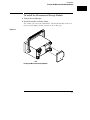
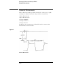
To install the Measurement/Storage Module
To install the Measurement/Storage Module
1 Turn off the oscilloscope.
2 Install the module as shown below.
The oscilloscope is reset after installation. The installed module is reflected
in the message displayed when you turn on the oscilloscope.
Figure 1–1
Installing the Measurement/Storage Module
1–3
Installation
To configure the interface
To configure the interface
The Measurement/Storage Module can be connected to a printer, a plotter, or
a computer through the interface. The 54657A has an GPIB interface and
the 54658A has an RS-232 interface. The 54659B has an RS-232 interface
plus an additional parallel output connector which allows the module to be
connected to both an RS-232 controller and a parallel printer at the same
time.
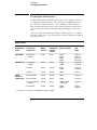
Connect the Measurement/Storage Module to a printer, plotter, or computer
through a suitable cable. The following table shows the Agilent part numbers
of the proper cables.
Interface Cables
Agilent Interface
module
Cable function
(Instrument to ..)
Module
connector
Printer/plotter/
controller
connector
Agilent part number
Cable
Length
54657A (GPIB)
Printer/plotter/
controller
HP-IB
HP-IB
10833A
10833B
10833C
10833D
1 m (3.3 ft)
2 m (6.6 ft)
4 m (13.2 ft)
0.5 m (1.6 ft)
54658A (RS-232)
Printer/plotter/
controller
25-pin F
25-pin F
13242G
17255M
5 m (16.7 ft)
1.5 m (4.9 ft)
Controller
25-pin F
25-pin M
92219J
17255D
5 m (16.7 ft
1.5 m (4.9 ft)
Controller
25-pin F
9-pin M
24542G
3 m (9.9 ft)
RS-232 controller
9-pin M
25-pin M
34398A
2.5 m (8.2 ft)
RS-232 controller
9-pin M
9-pin M
34398A
2.5 m (8.2 ft)
RS-232 printer/plotter/
controller
9-pin M
25-pin F
34398A + 34399A
adapter kit
2.5 m (8.2 ft)
Parallel printer
parallel
parallel
C2950A
C2951A
2 m (6.6 ft)
3 m (9.9 ft)
54659B1
(RS-232 and
parallel output)
1
The 54659B is not compatible with the 54600A, 54601A, 54602A, and 54610A.
1–4
Installation
To configure the interface
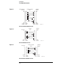
54658A Serial Connections
The signals for the RS-232 port on the 54658A are listed below.
Pin Number
2
3
4
5
6
7
8
20
SHELL
Signal
Transmit Data
Receive Data
Request to Send
Clear to Send
Data Set Ready
Signal Ground
Data Carrier Detect
Data Terminal Ready
Protective Ground
Figure 1– 2
Pin out of 54658A RS-232 port looking into DB25 female connector
The following figures show the pin outs of the suggested RS-232 interface
cables used with the 54658A 25-pin connector.
1–5
Installation
To configure the interface
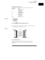
Figure 1– 3
13242G/17255M
Cable
Printer/plotter/
controller
54658A
Module
1
3
2
8
20
1
2
3
4
5
6
7
8
12
11
19
20
25-pin
female
7
4
19
11
12
5
6
25-pin
male
25-pin
male
25-pin
female
54645b09.cdr
Pin out of 13242G/17255M RS-232 cable
Figure 1– 4
54658A
Module
24542G
Cable
Controller
4
2
3
5
6
7
20
1
2
3
4
5
6
8
7
9-pin
male
8
25-pin
male
9-pin
female
25-pin
female
54657b10.cdr
Pin out of 24542G RS-232 cable
Figure 1– 5
1
2
3
5
6
7
20
25-pin
male
25-pin
female
Pin out of 92219J/ 17255D RS-232 cable
1–6
54658A
Module
92219J/17255D
Cable
Controller
1
3
2
20
7
5
6
25-pin
male
25-pin
female
54645b08.cdr
Installation
To configure the interface
54659B Serial Connections
The signals for the 9-pin RS-232 port on the 54659B are listed below.
Pin Number
1
2
3
4
5
6
7
8
9
SHELL
Signal
Data Carrier Detect
Receive Data
Transmit Data
Data Terminal Ready
Signal Ground
Data Set Ready
Request to Send
Clear to Send
Ring
Protective Ground
Figure 1– 6
Pin out of 54659B RS-232 port looking into DB9 male connector
The following figure shows the pin out of the suggested RS-232 interface
cable used with the 54659B 9-pin connector.
Figure 1– 7
Printer/Plotter/
Controller
DCD
RX
TX
DTR
GND
DSR
RTS
CTS
RI
9-pin
male
54659B
Module
34398A
Cable
1
2
3
4
5
6
7
8
9
9-pin
female
1
2
3
4
5
6
7
8
9
9-pin
female
DCD
RX
TX
DTR
GND
DSR
RTS
CTS
RI
9-pin
male
54657b07.cdr
Pin out of 34398A RS-232 cable
Refer to the "Programming over RS-232-C" chapter in the Agilent
54600–Series Oscilloscopes Programmer’s Guide for additional
information.
1–7
1–8
2
Operating the
Measurement/Storage Module
Operating the Measurement/Storage
Module
This chapter provides you with the information necessary to use the
additional, or enhanced features that the Measurement/Storage
Module provides. Basic operation for the oscilloscope is covered in
the User and Service Guide for your oscilloscope.
This chapter provides you with practical exercises and detailed
information designed to guide you through operation of the following
functions:
•
•
•
•
•
Math Functions
Automatic Measurements
Cursor Measurements
Mask generation and waveform monitoring
Trace Storage
2–2
Operating the Measurement/Storage Module
Math Functions
Math Functions
Without the Measurement/Storage module installed, addition and subtraction
are the only math operations provided. In addition to the limited selections,
the single function is performed on the pixel position of the data on the
screen.
With the Measurement/Storage module installed, two functions define up to
six operations that create mathematically altered waveforms (not pixel math.)
• Function 1 will add (+), subtract (–), or multiply (*) the signals acquired
on vertical inputs 1 and 2, then it will display the result as F1.
• Function 2 will integrate, differentiate, or perform an FFT on the signal
acquired on input 1, input 2, or the result in F1; then it will display the
result in F2.
The vertical range and offset of each function can be adjusted for ease of
viewing and measurement considerations. Each function can be displayed,
measured (with cursors), stored in trace memory, or output over the
interface.
2–3
Operating the Measurement/Storage Module
Function 1
Function 1
1 Press ± .
2 Toggle the Function 1 On Off softkey to enable math function number 1.
3 Press the Function 1 Menu softkey
A softkey menu with four softkey choices appears. Three of them are related
to the math functions.
4 Toggle the + – * softkey until the desired operation is selected.
Results (F1) are displayed on the screen.
All operations are calculated on a point-by-point basis.
• plus (+) algebraically sum input 1 and input 2 (input 1 + input 2).
• minus (–) algebraically subtract input 2 from input 1 (input 1 – input 2).
• multiply (*) algebraically multiply input 1 with input 2 (input 1 * input 2).
5 Press the Units/div softkey and rotate the knob closest to the
Cursors key to set the vertical sensitivity of the resulting
waveform.
6 Press the Offset softkey and rotate the knob closest to the
Cursors key to set the offset (from the center graticule) of the
resulting waveform.
Function waveform (F1) is available for viewing, measurement, or storage.
7 Press the Previous Menu softkey.
Function 1 Operating Hints
If channel 1 or 2 are clipped (not fully displayed on screen,) the resulting
displayed function will also be clipped. Once the function is displayed, channel
1 and 2 may be turned off for better viewing.
When multiply is the operation selected, the value displayed for units per
division and offset is (V2).
Offset is the value (in V or V2) assigned to the center graticule for function 1.
Normal screen position is 0 V offset, or at the center graticule (until changed).
See "Making Cursor Measurements", and "Saving and Recalling Traces" in this
chapter for more information.
2–4
Operating the Measurement/Storage Module
Function 2
Function 2
Function 2 will plot differential or integral waveforms, or perform an FFT
using the input signals connected to the vertical inputs (1 and 2), or using
the function 1 waveform.
1 Press ± .
2 Toggle the Function 2 On Off softkey to enable math function number 2.
3 Press the Function 2 Menu softkey.
4 Toggle the Operand softkey until the desired source is selected.
F1 uses the result waveform in function 1.
5 Press the Operation softkey until the desired operation is selected.
Results (F2) are displayed on the screen.
• dV/dt (differentiate) plots the derivative of the selected source using the
"Central Difference" formula. Equation is as follows:
cn–cn+1+2i
dn+i =
∆t(2i+1)
Where
d = differential waveform
c = input 1, 2, or function 1
i = data point step size
∆t = point-to-point time difference
• ∫dt (integrate) plots the integral of the source using the "Trapezoidal Rule".
Equation is as follows:
In =
∆t
(cn+cn+1)
2∑
Where
∆t = point-to-point time difference
c = input 1, 2, or function 1
2–5
Operating the Measurement/Storage Module
Function 2
The integrate calculation is relative to the currently selected source’s
input offset. The following examples illustrate any changes in offset
level.
Figure 2– 1
0V
0V
Integrate and Offset
•
FFT (Fast Fourier Transform) inputs the digitized time record of the source
and transforms it to the frequency domain. The FFT spectrum is plotted
on the oscilloscope display as dBV (dBV or dBm for 54610 and
54615/54616) versus frequency. Selecting this function also adds the FFT
Menu. See "FFT Measurement" later in this chapter for more information.
6 Press the Units/div softkey and rotate the knob closest to the
Cursors
key to set the vertical sensitivity of the resulting
waveform.
Units per division changes from volts to dB when FFT is selected.
2–6
Operating the Measurement/Storage Module
Function 2
7 Press the Offset (differentiate and integrate) or Ref Levl (FFT) softkey
and rotate the knob closest to the Cursors key to set the offset
(from the center graticule) or reference level (top graticule) of
the resulting waveform.
Function waveform (F2) is available for viewing, measurement, or storage.
8 Press the Previous Menu softkey.
For FFT functions, an additional menu is available to set additional
parameters. See "FFT Measurement" later in this chapter for more
information.
Function 2 Operating Hints
Timebase must be set to Main (and input channels 3 and 4 to Off on 4-channel
oscilloscopes) when using function 2.
When differential is the operation selected, the value displayed for units per
division and offset is volts per second (V/s). When integral is the operation
selected, the value displayed for units per division and offset is volt seconds
(Vs).
Offset is the value (in volts per second or volt seconds) assigned to the center
graticule for function 2. Normal screen position is 0 offset, or at the center
graticule (until changed).
See "Making Cursor Measurements", and "Saving and Recalling Traces" in this
chapter for more information.
2–7
Operating the Measurement/Storage Module
FFT Measurement
FFT Measurement
Operating System Requirements
Refer to "Oscilloscope Compatibility" on page 1-2 for operating system
requirements for FFT operation.
FFT (Function 2) is used to compute the fast Fourier transform using
vertical inputs (1 and 2), or the Function 1 waveform. This function takes
the digitized time record of the specified source and transforms it to the
frequency domain. When the function is selected, the FFT spectrum is
plotted on the oscilloscope display as dBV (dBV or dBm for 54610 and
54615/54616) versus frequency. The readout for the horizontal axis changes
from time to Hertz and the vertical readout changes from volts to dBV (dBV
or dBm for 54610 and 54615/54616). For the 54610 and 54615/54616, when
50Ω input is selected, readout is in dBm; when 1MΩ input is selected,
readout is in dBV. dBV is a unit of measure that is referenced to 1 Vrms. If
the display of the 54600, 54601, 54602, 54603, or 54645 is needed to be in
dBm, the operator must apply an external 50Ω load (10100C or equivalent),
and then perform the following conversion:
dBm = dBV + 13.01
DC Value The FFT computation produces a DC value that is incorrect.
It does not take the offset at center screen into account and is 1.41421
times greater than its actual value. The DC value is not corrected in
order to accurately represent frequency components near DC. All DC
measurements should be performed in normal oscilloscope mode.
2–8
Operating the Measurement/Storage Module
FFT Measurement
Aliasing When using FFT’s, it is important to be aware of aliasing. This
requires that the operator have some knowledge as to what the
frequency domain should contain, and also consider the effective
sampling rate, frequency span, and oscilloscope vertical bandwidth when
making FFT measurements. Effective sample rate is briefly displayed
when the ± key is pressed.
Aliasing happens when there are insufficient samples acquired on each cycle
of the input signal to recognize the signal. This occurs whenever the
frequency of the input signal is greater than the Nyquist frequency (sample
frequency divided by 2). When a signal is aliased, the higher frequency
components show up in the FFT spectrum at a lower frequency.
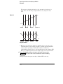
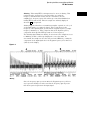
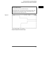
The following figure illustrates aliasing. In waveform A, the sample rate is set
to 200 kSa/s, and the oscilloscope displays the correct spectrum. In
waveform B, the sample rate is reduced by one-half (100 kSa/s), causing the
components of the input signal above the Nyquist frequency to be mirrored
(aliased) on the display.
Figure 2– 2
Aliasing
Since the frequency span goes from ≈ 0 to the Nyquist frequency, the best
way to prevent aliasing is to make sure that the frequency span is greater
than the frequencies present in the input signal.
2–9
Operating the Measurement/Storage Module
FFT Measurement
Spectral Leakage The FFT operation assumes that the time record
repeats. Unless there is an integral number of cycles of the sampled
waveform in the record, a discontinuity is created at the end of the
record. This is referred to as leakage. In order to minimize spectral
leakage, windows that approach zero smoothly at the beginning and end
of the signal are employed as filters to the FFT. The
Measurement/Storage Module provides four windows: rectangular,
exponential, hanning, and flattop. For more information on leakage, see
Agilent Application Note 243, "The Fundamentals of Signal Analysis"
(Agilent part number 5952-8898.)
FFT Operation
1 Press ± .
2 Toggle the Function 2 On Off softkey to enable math function number 2.
3 Press the Function 2 Menu softkey.
4 Toggle the Operand softkey until the desired source is selected.
F1 uses the result waveform in function 1.
5 Press the Operation softkey until FFT is selected. Results (F2) are
displayed on the screen.
6 Press the Units/div softkey and rotate the knob closest to the
Cursors key to set the vertical sensitivity of the resulting
waveform.
7 Press the Ref Levl softkey and rotate the knob closest to the
Cursors key to set the reference level (top graticule line) of
the resulting waveform.
The Autoscale FFT softkey will automatically set Units/div and Ref Levl to bring
the FFT data on screen. Frequency Span is set to maximum. Steps 6 and 7 could
be replaced to say:
6 Press FFT Menu softkey.
7 Press Autoscale FFT softkey. Rotate Time/Div knob until freq span is around
the frequencies of interest.
8 Press the FFT Menu softkey.
A softkey menu with six softkey choices appears. Five of them are related to
FFT.
2–10
Operating the Measurement/Storage Module
FFT Measurement
• Cent Freq Allows centering of the FFT spectrum to the desired frequency.
Select and rotate the knob closest to the Cursors key to set the
center frequency to the desired value.
• Freq Span Sets the overall width of the FFT spectrum (left graticule to
right graticule). Select and rotate the knob closest to the Cursors
key to set the center frequency to the desired value. See FFT
Measurement Hints (next page) for information on using frequency
span to magnify the display.
• Move 0Hz To Left Pressing this key changes the center frequency so that
the left most graticule represents 0 Hz.
• Autoscale FFT The Autoscale FFT softkey will automatically set Units/div
and Ref Levl to bring the FFT data on screen. Frequency Span is set to
maximum.
• Window Allows one of four windows to be selected. Select and rotate the
knob closest to the Cursors key to set the desired window. The
rectangular window is useful for transients signals and signals where
there are an integral number of cycles in the time record. The hanning
window is useful for frequency resolution and general purpose use. It
is good for resolving two frequencies that are close together or for
making frequency measurements. The flattop window is the best
window for making accurate amplitude measurements of frequency
peaks. The exponential window is the best window for transients
analysis.
• Previous Menu Returns you to the previous softkey menu.
FFT spectrum (F2) is available for viewing, measurement, or storage.
9 The Cursors key contains two additional selections that can be
used to measure or move the FFT spectrum. Press Cursors
then set the Source softkey to F2.
,
Find Peaks Pressing this key sets Vmarker1 and the start marker (f1) on the
peak with the highest amplitude and sets Vmarker2 and the stop marker (f2)
on the peak with the next highest amplitude. Marker values in dBV/dBm or
frequency (dependent on the active cursor)are automatically displayed at the
bottom of the oscilloscope screen. The difference in dBV/dBm (∆V) or
frequency (∆f) between the two peaks is also displayed.
Move f1 To Center Pressing this key changes the center graticule (or center
frequency) to the current f1 marker frequency. If f1 cannot be found, a
message is displayed on the screen.
2–11
Operating the Measurement/Storage Module
FFT Measurement
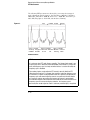
The following FFT spectrum was obtained by connecting the front panel
probe adjustment signal to input 1. Set Time/Div to 500 s/div, Volts/Div to
100 mV/div, Units/div to 10.00 dB, Ref Level to –10.00 dBV, Center Freq to
6.055 kHz, Freq Span to 12.21 kHz, and window to Hanning.
Figure 2– 3
fft(1)
6.05kHz 12.2kHz
1 STOP
f1(F2) = 1.221kHz
f2(F2) = 3.662kHz
f(F2) = 2.441kHz
Cent Freq Freq Span Move 0Hz Autoscale Window Previous
6.055kHz 12.21kHz
To Left
FFT
Hanning
Menu
FFT Measurements
FFT Measurement Hints
It is easiest to view FFT’s with Vectors set to On. The Vector display mode is set
in the Display menu. Note that on the 54615/54616, when Vectors is set from Off
to On, the frequency span is halved, and when Vectors is set from On to Off, the
frequency span is doubled.
The number of points acquired for the FFT record is normally 1024 (see FFT
"Operating Characteristics" in Chapter 3 for specifics,) and when frequency span
is at maximum, all points are displayed. Once the FFT spectrum is displayed, the
frequency span and center frequency controls are used much like the controls
of a spectrum analyzer to examine the frequency of interest in greater detail.
Place the desired part of the waveform at the center of the screen and decrease
frequency span to increase the display resolution. As frequency span is
decreased, the number of points shown is reduced, and the display is magnified.
2–12
Operating the Measurement/Storage Module
FFT Measurement
FFT Measurement Hints – Continued
While the FFT spectrum is displayed, use the and Cursor keys to switch between
measurement functions and frequency domain controls in FFT menu. See the
end of the manual for display menus.
Decreasing the effective sampling rate by selecting a slower sweep speed will
increase the low frequency resolution of the FFT display and also increase the
chance that an alias will be displayed. The resolution of the FFT is one-half of
the effective sample rate divided by the number of points in the FFT. The actual
resolution of the display will not be this fine as the shape of the window will be
the actual limiting factor in the FFT’s ability to resolve two closely space
frequencies. A good way to test the ability of the FFT to resolve two closely
spaced frequencies is to examine the sidebands of an amplitude modulated sine
wave. For example, at 2 MSa/sec effective sampling rate, a 1 MHz AM signal
can be resolved to 2 kHz. Increasing the effective sampling rate to 4 MSa/sec
reduces the resolution to 5 kHz.
For the best vertical accuracy on peak measurements:
• Make sure the source impedance and probe attenuation is set correctly.
The impedance and probe attenuation are set from the Channel menu if
the operand is a channel.
• Set the source sensitivity so that the input signal is near full screen, but
not clipped.
• Use the flattop window.
• Set the FFT sensitivity to a sensitive range, such as 2 dB/division.
For best frequency accuracy on peaks:
• Use the Hanning window.
• Use cursors to place f1 cursor on the frequency of interest.
• Press Move f1 to Center softkey.
• Adjust frequency span for better cursor placement.
• Return to the Cursors menu to fine tune the f1 cursor.
For more information on the use of window please refer to Agilent Application
Note 243," The Fundamentals of Signal Analysis" Chapter III, Section 5 (Agilent
part number 5952-8898.) Additional information can be obtained from "Spectrum
and Network Measurements" by Robert A Witte, in Chapter 4 (Agilent part
number 5960-5718.)
2–13
Operating the Measurement/Storage Module
Automatic Measurements
Automatic Measurements
With the Measurement/Storage Module installed, the oscilloscope is capable
of making five additional automatic voltage and time measurements.
•
•
•
•
•
Delay Measurements
Phase Measurements
Voltage Amplitude
Voltage Overshoot
Voltage Preshoot
In addition to the measurements, the thresholds used for automatic time
measurements are user-selectable.
Figure 2– 4
Automatic Measurements
2–14
Operating the Measurement/Storage Module
Setting Thresholds
Setting Thresholds
Without the Measurement/Storage module installed, rise time and fall time
measurements are performed at the 10%/90% threshold levels. The
remaining five time measurements (frequency, period, duty cycle, positive
pulse width, and negative pulse width) are all performed at the 50%
transition point. Refer to the User and Service Guide for your oscilloscope
for more information.
With the Measurement/Storage module installed, the thresholds are user
selectable. Rise time and fall time measurements are performed at 10%/90%,
20%/80%, or at a user defined threshold level. The remaining five time
measurements are performed at the center point of the currently selected
upper and lower threshold values.
• If 10%/90% is selected, the center is 50%.
• If 20%/80% is selected, the center is 50%.
• If voltage is selected, the center is dependent on the current lower and
upper values.
As an example, if the lower value is set to 0 V, and the upper value is set to
50 mV, then the 50% level is 25 mV. 25 mV is the point that frequency,
period, duty cycle, positive pulse width, and negative pulse width will be
measured. The point of measurement is dependent on the amplitude of the
input signal.
2–15
Operating the Measurement/Storage Module
Setting Thresholds
Figure 2– 5
User Thresholds
1 Press Time .
2 Press the Next Menu softkey until the Define Thresholds softkey is
displayed on the far left side.
3 Press the Define Thresholds softkey.
4 Press the desired Thresholds softkey.
A softkey menu with six softkey choices appears. Five of them are related to
selecting thresholds.
• 10% 90% Rise time/fall time measurements performed at the 10% (lower)
and 90% (upper) levels. Frequency, period, duty cycle, positive pulse
width, and negative pulse width measurements will be performed at the
50% level.
• 20% 80% Rise time/fall time measurements performed at the 20% (lower)
and 80% (upper) levels. Frequency, period, duty cycle, positive pulse
width, and negative pulse width measurements will be performed at the
50% level.
2–16
Operating the Measurement/Storage Module
Setting Thresholds
• Voltage Rise time/fall time measurements performed at the lower and
upper levels specified by you. Frequency, period, duty cycle, positive
pulse width, and negative pulse width measurements will be performed at
the center of both entered levels.
• Lower This softkey is displayed only when Voltage softkey is selected.
Select and rotate the knob closest to the Cursors key to set the
lower threshold to the desired value.
• Upper This softkey is displayed only when Voltage softkey is selected.
Select and rotate the knob closest to the Cursors key to set the
upper threshold to the desired value.
• Previous Menu Returns you to the previous softkey menu.
Selecting User Threshold Hints
Lower threshold level cannot be set to a value higher than the current upper
threshold level.
Upper threshold level cannot be set to a value lower than the current lower
threshold level.
If the upper and lower thresholds are set to levels greater to, or less than, the
current displayed waveform, then the automatic rise time, fall time, frequency,
period, duty cycle, positive pulse width, and negative pulse width measurements
will not be performed. This is because the measurement point is not on the
waveform.
Cursors can be used to set the threshold voltage levels as follows:
• Select an automatic time measurement with Show Meas set to On, and
thresholds set to 10%/90%. Once initiated, the cursors will display on the
waveform.
• Press Cursors key and record the current cursor voltage levels.
• Select Define Measurement Voltage, and adjust the upper and lower levels
to the previously recorded values.
• Slowly rotate the knob closest to the Cursors key to fine tune the upper and
lower threshold to the desired values. Cursor will track as long as the
measurement is valid.
2–17
Operating the Measurement/Storage Module
Setting Thresholds
Figure 2– 6
User Threshold Rise Time Measurement
2–18
Operating the Measurement/Storage Module
To make delay measurements automatically
To make delay measurements automatically
You can measure the delay of signals connected to the oscilloscope’s input 1
and input 2 connectors when the Measurement/Storage Module is connected
to the oscilloscope.
Delay is measured from the user-defined slope and edge count of the signal
connected to input 1, to the defined slope and edge count of the signal
connected to input 2.
1 Adjust controls so that a minimum of 6 full cycles of the signals
connected to inputs 1 and 2 are displayed.
2 Press Time .
3 Press the Next Menu softkey until the Define Thresholds softkey is
displayed on the far left side.
4 Press the Define Delay softkey.
A softkey menu with five softkey choices appears. Four of them are related
to defining the delay measurement.
• Chan 1 Selects the channel 1 slope (rising or falling) where the delay
measurement will START. Threshold level is always 50%.
• Edge Selects the edge count (from 1 to 5) where the delay measurement
will START.
• Chan 2 Selects the channel 2 slope (rising or falling) where the delay
measurement will STOP. Threshold level is always 50%.
• Edge Selects the edge (from 1 to 5) count where the delay measurement
will STOP.
• Previous Menu Returns you to the previous softkey menu.
5 Use the displayed softkeys to specify the starting (from) and stopping
(to) slope and edge count. Transition point (measurement threshold
level) is fixed at 50%.
6 Press the Previous Menu softkey.
2–19
Operating the Measurement/Storage Module
To make delay measurements automatically
7 Press the Measure Delay softkey. Delay is measured and displayed on
the screen.
Negative delay values indicate the defined edge on channel 1 occurred after
the defined edge on channel 2.
Automatic Delay Measurement Hints
If an edge is selected that is not displayed on the screen, delay will not be
measured.
User thresholds have no effect on automatic delay measurements. Delay is
always measured at the 50% transition point (measurement threshold level).
Figure 2– 7
Automatic Delay Measurement
2–20
Operating the Measurement/Storage Module
To make phase measurements automatically
To make phase measurements automatically
Phase shift between two signals can be measured using the Lissajous method.
Refer to the User and Service Guide for your oscilloscope for more
information.
With the Measurement/Storage Module installed, phase is automatically
measured and displayed. Measurement is made from the rising edge of the
first full cycle on the input 1 signal, to the rising edge of the first full cycle on
the input 2 signal. The method used to determine phase is to measure delay
and period, then calculate phase as follows:
delay
Phase =
x 360
period of input 1
1 Adjust controls so that a minimum of one full cycle of the signal
connected to input 1 is displayed.
2 Press Time .
3 Press the Next Menu softkey until the Define Thresholds softkey is
displayed on the far left side.
4 Press the Measure Phase softkey. Phase is measured and displayed on
the screen.
Negative phase values indicate the displayed signal on channel 2 is leading
the signal on channel 1.
Automatic Phase Measurement Hints
If one full cycle of the signal connected to input 1 is not displayed, phase will not
be measured.
User thresholds has no effect on automatic phase measurements. Phase is
always measured at the 50% transition point (threshold level).
When using the delayed timebase, the instrument will attempt to perform the
measurement using the delayed window. If the selected channel 1 edge,
channel 2 edge, and channel 1 period cannot be found in the delayed window,
the main window is used. See "Time Measurements" in the User and Service
Guide for your oscilloscope for more information.
2–21
Operating the Measurement/Storage Module
To make phase measurements automatically
Figure 2– 8
Automatic Phase Measurement
2–22
Operating the Measurement/Storage Module
To make additional voltage measurements automatically
To make additional voltage measurements
automatically
With the Measurement/Storage Module is installed, the following additional
automatic voltage measurements can be performed.
• Vamplitude Amplitude Voltage measurement is made using the entire
waveform. When performing a measurement on a particular cycle, set the
controls to display only that cycle is displayed. The method used to
determine voltage amplitude is to measure Vtop and Vbase, then calculate
voltage amplitude as follows:
voltage amplitude = Vtop – Vbase
• Vovershoot A minimum of one edge must be displayed in order to perform
an Overshoot measurement. If more than one waveform, edge, or pulse is
present, the measurement is made on the first edge acquired. The method
used to determine overshoot is to make three different voltage
measurements, then calculate overshoot as follows:
percent overshoot =
Vmax–Vtop
x 100
Vtop–Vbase
• Vpreshoot A minimum of one edge must be displayed in order to perform
a Preshoot measurement. If more than one waveform, edge, or pulse is
present, the measurement is made on the first edge acquired. The method
used to determine preshoot is to make three different voltage
measurements, then calculate preshoot as follows:
Vmin–Vbase
x 100
percent preshoot =
Vbase–Vtop
2–23
Operating the Measurement/Storage Module
To make additional voltage measurements automatically
1 Adjust controls until the desired signal is displayed.
2 Press Voltage .
3 Press the Source softkey until the desired source is selected.
4 Press the Next Menu softkey until the Vamp softkey is displayed on the
far left side.
5 Press the desired Voltage Measurement softkey.
• Vamp Select to perform a voltage amplitude measurement.
• Vover Select to perform an overshoot measurement.
• Vpre Select to perform a preshoot measurement.
Figure 2– 9
Automatic Overshoot Measurement
2–24
Operating the Measurement/Storage Module
To make additional cursor measurements
To make additional cursor measurements
Without the Measurement/Storage Module installed, cursor measurements
can be performed on channels 1 through 4, and are displayed in volts (V1/V2)
and time (t1/t2). Refer to the User and Service Guide for your oscilloscope
for more information.
With the Measurement/Storage Module installed, additional cursor
measurement features include:
• Measurements can now be performed on functions 1 and 2.
• You can define voltage marker units as either volts or relative percent.
• You can define the time units as either seconds or relative degrees.
1 Adjust controls until the desired signal is displayed.
2 Press Cursors .
3 Toggle the Source softkey until the desired source is selected
(channels 1 through 4, functions 1 and 2).
4 Press the Active Cursor V1 V2 softkey.
5 Toggle the Readout softkey to select voltage markers in percent.
If Readout Volts is selected, cursor measurements are displayed in volts (V1,
V2, and ∆V), and operation is identical as when the module is not installed.
Refer to the User and Service Guide for your oscilloscope for more
information.
6 Toggle the Active Cursor V1 V2 softkey until the desired marker(s) (V1,
V2, or both) are selected, and rotate the knob closest to the
Cursors key to set the marker(s) to the desired position.
When both V1/V2 markers are selected, rotating the knob closest to the
Cursors key moves both markers.
7 Press the Set 100% softkey to set the V1 marker to 0% and the V2
marker to 100%. All readings are now relative to the established
V1/V2 marker positions.
• V1 reads the percentage the V1 marker has moved from the established
0% position. Negative readings indicate marker has moved away from the
V2 marker.
2–25
Operating the Measurement/Storage Module
To make additional cursor measurements
• V2 reads the percentage the V2 marker has moved from the established
100% position. Negative readings indicate marker has moved through the
established V1 marker position.
• ∆V reads the percentage difference between the V1 and V2 marker
repetitive to the established positions. Negative readings indicate markers
have crossed.
Figure 2– 10
Voltage Cursor Measurements in Percent
8 Press the Active Cursor t1 t2 softkey.
9 Toggle the Readout softkey to select time markers in degrees.
If Readout Time is selected, cursor measurements are displayed in seconds
(t1, t2, and ∆t), and Hz (1/∆t). Operation is identical as when the module is
not installed. Refer to the User and Service Guide for your oscillosocpe for
more information.
10 Toggle the Active Cursor t1 t2 softkey until the desired marker(s) (t1, t2,
or both) are selected, and rotate the knob closest to the
Cursors key to set the marker(s) to the desired position.
When both t1/t2 markers are selected, rotating the knob closest to the
Cursors key moves both markers.
2–26
Operating the Measurement/Storage Module
To make additional cursor measurements
11 Press the Set 100% softkey to set the t1 marker to 0° and the t2 marker
to 360°. All readings (except second ∆t display in seconds) are now
relative to the established t1/t2 marker positions.
• t1 reads the phase the t1 marker has moved from established 0° position.
Negative readings indicate marker has moved away from the t2 marker.
• t2 reads the phase the t2 marker has moved from established 360°
position. Negative readings indicate marker has moved through the
established t1 marker position.
• ∆t in degrees reads the phase difference between the t1 and t2 marker
repetitive to the established positions. Negative readings indicate markers
have crossed.
• ∆t in seconds reads the time difference between the t1 and t2 marker
positions. Negative readings indicate markers have crossed.
Additional FFT Function Keys
When the FFT function is selected (refer to Math Functions), two additional keys
are available as follows:
Find Peaks Pressing this key sets Vmarker1 and the start marker (f1) on the FFT
trace peak with the highest amplitude and sets Vmarker2 and the stop marker
(f2) on the peak with the next highest amplitude. Marker values in dBV or
frequency (dependent on the active cursor)are automatically displayed at the
bottom of the oscilloscope screen. The difference in dBV (∆V) or frequency ( ∆f)
between the two peaks is also displayed.
Move f1 To Center Pressing this key changes the center graticule (or center
frequency) to the current f1 marker frequency. If f1 cannot be found, a message
is displayed on the screen.
2–27
Operating the Measurement/Storage Module
To make additional cursor measurements
Cursor Measurement Hints
If cursors are positioned too closely together, an error will be displayed when
the SET softkey is selected.
Displayed marker readings in percent (%) and degrees (°) are always relative
measurements, with the current reading dependent on the previously
established 100% or 360 reference setting.
Figure 2– 11
Time Cursor Measurements in Degrees
2–28
Operating the Measurement/Storage Module
Unattended Waveform Monitoring
Unattended Waveform Monitoring
The Measurement/Storage Module simplifies circuit debugging by comparing
an active channel (not functions) trace on the display to one of two test
templates.
When a failure is detected, the oscilloscope can be instructed to take one of
several actions.
• The test can be set to stop after the first failure, or to continue regardless
of the number of failures found.
• The failed trace(s) can be stamped with the date and time of the failure,
and stored in trace memory or output to a hardcopy device. When trace
memory is selected, the user has the option of saving all failures, or saving
only the last failure that occurred.
• The test can continue with statistics on the number of failures (reported
as a percentage of the number of tests performed) being displayed.
The mask templates can be defined one of two ways. Once a mask is created,
it is stored in nonvolatile RAM.
• Automask Quickly generates a mask template from currently displayed
data. You are allowed to select the mask tolerance prior to creating the
template.
• Editor Used to adjust the tolerances of a previously created template in
areas of specific interest, or to create a complete new mask. Mask editor
allows pixel-by-pixel editing, and smoothing of the mask by using a
running average of three pixels.
Failures can be specified one of two ways.
• Inside Test fails if signal falls inside the region defined by the maximum
and minimum limit lines of the mask template.
• Outside Test fails if signal falls outside the region defined by the
maximum and minimum limit lines of the mask template.
2–29
Operating the Measurement/Storage Module
To create a mask template using Automask
To create a mask template using Automask
A mask template contains two limit lines: minimum and maximum.
Automask allows you to easily generate a mask with tolerances from a
displayed waveform on the screen.
1 Connect a known good signal to the oscilloscope.
2 Set up the oscilloscope with the settings that are required to test the
signal.
3 Press ± .
4 Press the Mask Test softkey.
5 Toggle the Use Mask softkey to select the desired mask number
(1 or 2).
6 Press the Define Mask Automask softkey.
7 Press the Tolerance softkey, then turn the knob closest to the
Cursors
key to set the tolerance.
Pressing the softkey increases the tolerance value by 0.2%.
8 Press the Create Mask softkey to create the mask with the specified
tolerance.
Tolerance Operating Hint
The tolerance used in Automask is expressed as a percentage of the full-scale
time and voltage of the lowest number of all active channels. It does not
represent the tolerance of the actual size of the input signal. To specify the
tolerance as a percentage of the actual size of the input signal requires some
additional calculations.
For example, a signal of 1 volt peak-to-peak is tested at a vertical sensitivity of
500 mV/div. The full-scale voltage equals the volts/div times the number of
full-scale divisions (500 mV * 8 = 4 V). To specify a 4% tolerance on a 1 V
peak-to-peak signal requires a 40 mV tolerance, but to specify a 40 mV tolerance
on a full-scale voltage of 4 volts requires a 1% tolerance. Therefore, a 1%
tolerance should be specified to generate the mask template.
2–30
Operating the Measurement/Storage Module
To create a mask template using Autostore
To create a mask template using Autostore
An envelope of the passing region can be generated using the Autostore
function. Then the Automask function can read the Autostore screen
information and take the maximum and minimum limits of it as the limit lines
of the mask template. This process allows you to create a mask template
from a known good signal, allowing certain tolerance margins.
1 Connect a known good signal to the oscilloscope.
2 Set up the oscilloscope with the settings that are required to test the
signal.
3 Press Display , then toggle the Grid softkey to the None
position.
4 Press Autostore .
Make sure that STORE is displayed in the status line. If STORE is not
displayed, press Autostore again.
5 Set the voltage tolerance by moving the waveform up and down with
the vertical position knob, creating a vertical envelope.
6 Set the time tolerance by moving the waveform back and forth with
the horizontal delay knob, creating a horizontal envelope.
You may need to repeat steps 5 and 6 to fine tune the envelope. Cursors can
be used to accurately measure the margins.
An alternative method is to vary the input signal amplitude (level) and
frequency (time) by the desired amount.
7 Press ± .
8 Press the Mask Test softkey.
9 Press the Use Mask softkey to select the desired mask number (1 or 2).
10 Press the Define Mask Automask softkey.
2–31
Operating the Measurement/Storage Module
To create a mask template using Autostore
11 Press the Tolerance softkey, then turn the knob closest to the
Cursors
key to set the tolerance to ±0.0%.
If additional tolerance is desired, set the tolerance to the appropriate level.
This will be the amount "added on" to the previously created envelope.
12 Press the Create Mask softkey to create the mask from the autostore
information.
Automask Using Autostore Operating Hint
The Automask function takes all the information displayed in half bright to create
the mask. However, the display grid and the autostore information shares the
same half-bright display. If the grid is turned on, and Autostore information is on
the screen when the Create Mask softkey is pressed, a warning message is
displayed: "Grid must be None to generate mask with Autostore." The Display
Grid must be turned to None prior to creating the autostore data in order to use
Automask function. Turning the grid to None after the autostore data is created
erases both the grid and the autostore data. Use of cursors does not affect the
Automask function and is highly recommended to ensure the proper testing
margin in the autostore information.
If there is noise rising on the limit lines, you can use the smooth function in the
mask editor to smooth out the noise.
2–32
Operating the Measurement/Storage Module
To create or edit a mask using line segments
To create or edit a mask using line segments
The Measurement/Storage Module has a built-in Mask Editor for creating or
editing masks. It provides two editing tools: pixel editing and line drawing
editing. The line drawing editing tool can also be used to create a mask using
line segments.
To create the mask, you may want to first draw the mask on a piece of paper
and mark the coordinates of the end points of each straight line.
1 Press ± .
2 Press the Mask Test softkey.
3 Press the Use Mask softkey to select the desired mask number (1 or 2).
4 Press the Define Mask Editor softkey.
A softkey menu with five softkey choices appears. Four of them are related
to the mask editing functions.
If a mask has been previously created, it will be displayed.
• Edit Line Selects the limit line to be edited. Minimum is selected to edit
the bottom limit line, and maximum is selected to edit the top limit line.
• Line Drawing - Mark and Connect Mark and Connect are used for drawing
straight lines in the mask. Their operation is explained later in this
paragraph.
• Smooth Mask A running average of three pixels is used to smooth the
mask. It is especially useful for smoothing a mask created by Automask,
which may contain noise on the mask.
Each time Smooth Mask is selected, the entire mask is updated.
Selecting smoothing numerous times can alter the desired mask
pattern.
• Previous Menu Returns you to the previous softkey menu.
2–33
Operating the Measurement/Storage Module
To create or edit a mask using line segments
5 Toggle the Edit Line softkey to select the limit line you want to edit.
6 Turn the Delay knob to move the X-coordinate of the cursor to the
time corresponding to the first point.
If a mask has been previously created, both the X and Y coordinate of the
cursor will track the selected limit line.
7 Turn the knob closest to the Cursors key to move the
8
9
10
11
12
Y-coordinate of the cursor to the voltage corresponding to the
first point.
Press the Mark softkey to mark this point as the first point of a line
draw.
Turn the delay knob to move the X-coordinate of the cursor to the
time corresponding to the second point.
Turn the knob closest to the Cursors key to move the
Y-coordinate of the cursor to the voltage corresponding to the
second point of the line.
Press the Connect softkey to draw the line between both points.
Repeat procedures 5 through 11 until the desired mask is created.
Mask Editor Operating Hint
When you want to move the cursor to a particular location, it is essential to first
move the X-coordinate of the cursor then the Y-coordinate. Otherwise, the
movement of the Y-coordinate changes the position of a pixel at an undesired
location.
After you press the Connect softkey, the two points are connected by a straight
line. Points between the two end points are interpolated. However, if the
voltage of a particular point during interpolation violates the rule of the voltage
at the maximum limit ≥ the voltage at the minimum limit, the voltage is set to the
same value as the other limit.
After you have marked the first point, pressing the Mark softkey again cancels
the previously marked point and starts the procedure over.
After you have connected the two points, pressing the Connect softkey again
will undo the connect operation.
2–34
Operating the Measurement/Storage Module
To edit an individual pixel of a mask
To edit an individual pixel of a mask
Previously created masks can be edited pixel-by-pixel using the line drawing
editing tool. The Delay knob selects the column to be edited, and the
Cursors knob moves the mask vertically.
1 Press ± .
2 Press the Mask Test softkey.
3 Press the Use Mask softkey to select the desired mask number (1 or 2).
4 Press the Define Mask Editor softkey.
5 Toggle the Edit Line softkey to select the limit line that you want to
edit.
6 Turn the Delay knob to move the cursor to the pixel (column) that
you want to modify.
7 Turn the knob closest to the Cursors key to edit the vertical
position of the pixel.
It is possible to repeat steps 6 and 7 (simultaneously) using two hands to
create a nice smooth mask.
Pixel Editing Operating Hint
The time and voltage shown at the bottom of the screen corresponds to the
current time base and vertical setting of lowest number of all active channels. If
the mask is voltage and time dependent, make sure that the current time base
and vertical setting are the same as the one that you are going to use during the
actual testing.
Once the Cursor knob is moved, the selected pixel is edited. To remove
undesired edits, use the mark and connect softkeys (previously discussed).
2–35
Operating the Measurement/Storage Module
To edit the mask to test only a portion of a waveform
To edit the mask to test only a portion of a waveform
In certain circumstances, not all the points on the waveform need to be
tested. Only the area of interest needs to be tested. For example, to test the
amount of overshoot of a pulse, you only need to test the portion of the
waveform after the rising edge. You can select the test region by editing the
shape of the mask template.
1 Press ± .
2 Press the Mask Test softkey.
3 Press the Use Mask softkey to select the desired mask number (1 or 2).
4 Press the Define Mask Editor softkey.
5 Toggle the Edit Line softkey to select the limit line that you want to
edit.
6 Turn the Delay knob to move the cursor to the starting location that
7
8
9
10
11
you do not want to test.
Turn the knob closest to the Cursors key to move the voltage
cursor until it reads "Don’t Care".
Press the Mark softkey.
Turn the Delay knob to move the cursor to the ending location of the
region that you do not want to test.
Turn the knob closest to the Cursors key to move the voltage
cursor until it reads "Don’t Care".
Press the Connect softkey.
This region of this particular limit line is not tested during the mask testing.
2–36
Operating the Measurement/Storage Module
To edit the mask to test only a portion of a waveform
Mask Editing Operating Hint
Each limit line can have its own selectable test region.
The figure below shows a mask that tests the overshoot of the waveform. Note
that only the part you are interested in is tested. The test region can be set
individually for the maximum and minimum limit.
Figure 2– 12
Example mask template with selectable test region
2–37
Operating the Measurement/Storage Module
To start waveform monitoring
To start waveform monitoring
Before using a testing mask to monitor a waveform, the mask must be
created. Once created, the mask is automatically stored in one of the two
nonvolatile mask memories. Procedures for creating a mask template are
provided in this chapter.
1 Press ± .
2 Press the Mask Test softkey.
3 Press the Use Mask softkey to select the previously created mask
number (1 or 2).
4 Press the Test Options softkey.
A softkey menu with six softkey choices appears. Five of them are related to
the mask testing functions.
• Fail When – In or Out Selects if a test failure occurs when the signal moves
out of, or in to the mask template.
• On Fail - Stop or Run Used to select what state the oscilloscope will be in
after a test violation has occurred.
When stop is selected, the current acquisitions stop when the first
violation of the mask occurs. The test can be restarted by pressing
the RUN key.
When run is selected, the oscilloscope continues to acquire data
and display the most recent trace.
• Auto Save – Off or On Used to select if a test violation waveform is
recorded. When On is selected, an additional softkey appears. See
"Automatically Saving Test Violations" later in this chapter for more
information.
• Save To This softkey is displayed only when Auto Save On is selected.
Toggle softkey to direct test failure data to the Trace memory, or to the
Printer. When Trace is selected, an additional softkey appears.
2–38
Operating the Measurement/Storage Module
To start waveform monitoring
• Increment This softkey is displayed only when Save To Trace is selected.
When On, all test violations are saved by incrementing the trace
number. The starting trace number is the one that is currently
selected. When the 64K compressed memory is full, the oldest
trace memory is overwritten, and the trace count continues
incrementing. When the trace count reaches 100, the number
resets to 1 (wraps around).
When Off, only the last test violation is saved, as test failure data is
written over previously stored data.
• Previous Menu Returns you to the previous softkey menu.
5 Toggle the softkeys to select the desired testing options.
6 Press the Previous Menu softkey.
7 Press the Mask Test softkey until On is selected.
Selecting on immediately starts the test using the test options specified. Test
indications are displayed on the display line as follows.
• Pass Indicates the displayed waveform passed the test.
• Fail Indicates the displayed waveform failed the test. Further testing,
and disposition of the failed data is dependent on the testing options
selected.
• Acquisitions Indicates the total acquisitions made during the test.
• Failures Indicates the total number (and percentage) of test failures that
occurred during the test.
Waveform Monitoring Operating Hint
Mask template testing can only be used in the Main Horizontal Mode, and when
Functions 1 and 2 are set to off.
The trace review softkey can be used to review all saved failures. See "To Save
or Recall Traces" in this chapter for more information.
2–39
Operating the Measurement/Storage Module
To automatically save test violations
To automatically save test violations
The signals that fail the waveform monitoring test can be saved, then
viewed/measured at a later time. Provisions are provided to save the
violations in trace memory, or print a hardcopy of the data. When trace is
selected, the option of saving only the last violation, or saving all violations
are provided.
1 Setup for waveform monitoring as described previously.
2 Press ± .
3 Press the Mask Test softkey.
4 Press the Test Options softkey.
5 Press the Auto Save softkey to ON. This causes the Save To softkey to appear.
Determine how the test violations are being saved, and proceed as follows:
• To print test violation data on an externally connected printer, toggle the
Save To softkey until Print is selected.
• To save test violation data in trace memory, toggle the Save To softkey
until Trace is selected. This causes the Increment softkey to appear.
• To save only the last test violation waveform in trace memory, toggle the
Increment softkey until Off is selected.
• To save all test violation waveforms in trace memory, toggle the Increment
softkey until On is selected.
6 Press the Previous Menu softkey.
7 Press the Mask Test softkey until On is selected.
2–40
Operating the Measurement/Storage Module
To automatically save test violations
Saving Test Violation Data Operating Hint
When Increment On is selected, traces ≥3 to 100 are stored in the compressed
state. During the compression and storage of data, new signals are not
acquired or tested. The time it takes to compress and store data is less than 10
seconds.
When Increment On is selected, and multiple violations are desired, the On Fail
softkey must be set to Run (in the Test Options menu). The starting trace number
is the one that is currently selected. When the 64K compressed memory is full,
the oldest trace memory is overwritten, and the trace count continues
incrementing. When the trace count reaches 100, the number resets to 1 (wraps
around).
2–41
Operating the Measurement/Storage Module
Creating a delay testing mask
Creating a delay testing mask
A mask can be used to test the channel to channel delay of two input signals.
The shape of the mask varies depending on the channel 2 edge selected (stop
edge). Different masks are needed for different edge selections.
To test the channel to channel delay of the signal connected to channel 2, the
stop edge of the signal is tested instead of actually measuring the delay. The
test can be conducted by triggering on the start edge (channel 1), and testing
for the location of the stop edge (channel 2). An example mask is shown in
the following figure.
Figure 2– 13
Example of a mask template used in channel to channel delay
2–42
Operating the Measurement/Storage Module
Creating a delay testing mask
The following procedure can be used to setup a mask template for testing
channel to channel delay.
In the oscilloscope setup, the controls should be selected to display the start
edge (channel 1) as the first edge on the display, and the stop edge
(channel 2) as the last edge on the display. The trigger source should be set
to trigger from channel 1. The mask template can be created by using an
external signal source to generate the signals identical to the ones that are
going to be tested.
1 Connect the desired signals to the oscilloscope.
2 Set the signal source(s) to generate a waveform identical to the ones
that you are going to test.
3 Press ± on the oscilloscope, then press the Mask Test softkey.
4 Create a mask (at the desired tolerance) using Automask. Press
Previous Menu softkey when finished.
Refer to "Create a Mask Template Using Automask" for more information on
using automask.
5 Press the Define Mask Editor softkey.
6 Toggle the Edit Line softkey to select the Min limit line. Use the Mark
and Connect softkeys to edit the minimum line so only the last edge is
present (refer to previous figure).
Refer to "Create or Edit a Mask Using Line Segments" for additional
information.
7 Toggle the Edit Line softkey to select the Max limit line. Use the Mark
and Connect softkeys to edit the minimum line so only the first edge is
present (refer to previous figure). Press Previous Menu softkey when
finished.
2–43
Operating the Measurement/Storage Module
Creating a frequency testing mask
Creating a frequency testing mask
A mask can be used to test the frequency of the input signal. The shape of
the mask varies depending on the shape of the signal to be tested. A mask
designed for testing a sine wave cannot be used to test a square wave.
Different masks are needed for different shapes of signals. Using the
calibrated vertical vernier, position, and time base of the
Agilent 54600–Series oscilloscope, a mask can be re-used to test signals of
similar shapes but different frequencies and amplitudes.
To test the frequency of the signal, the period of the signal is tested instead
of actually measuring the frequency. The test can be conducted by triggering
on an edge of the signal and testing for the location of the second edge. An
example mask is shown in the following figure.
Figure 2– 14
Example mask for testing the frequency of a sine wave
2–44
Operating the Measurement/Storage Module
Creating a frequency testing mask
The following procedure can be used to setup a mask template for testing the
frequency of a sine wave or a square wave. Similar methods can be used to
generate masks for testing the frequency of signals of other shapes.
In the oscilloscope setup, the vertical sensitivity and position should be
adjusted so that the amplitude is almost full scale. The trigger level should
be adjusted to the middle of the input signal. The mask template can be
created by using a function generator to generate a signal of variable
frequency but of similar shape and amplitude to the one that is going to be
tested.
1 Connect the output of a function generator to the oscilloscope.
2 Set the function generator to generate a waveform with a similar
shape to the one that you are going to test.
3 Adjust the amplitude of the output until it is similar to the signal that
you are going to test.
4 Press Time on the oscilloscope, then press the Freq softkey to
turn on the automatic measurement for frequency.
5 Adjust the frequency of the output of the function generator to the
lower test limit.
The frequency can be verified by the automatic measurement.
6 Press Autostore .
7 Adjust the frequency of the output of the function generator to the upper test
limit.
An envelope of the test limit is generated.
8 Create a mask in the Define Automask menu with a tolerance of 0.0%.
For more information, refer to "To Create a Mask Template Using Autostore"
in this chapter.
9 Specify your test region in the Mask Editor menu.
2–45
Operating the Measurement/Storage Module
Creating an overshoot testing mask
Creating an overshoot testing mask
There are two parameters associated with the overshoot of a signal: the
percentage of overshoot and the settling time of the overshoot. A mask
template can be created to test the upper limit of these two parameters at
the same time. The following figure shows an example of a mask template for
testing overshoot.
Figure 2– 15
Example of a mask template for testing overshoot
2–46
Operating the Measurement/Storage Module
Creating an overshoot testing mask
The critical factors for creating the mask template are:
• The vertical window of the middle region of the mask template determines
the upper limit of the overshoot.
• The horizontal window of the middle region determines the upper limit of
the settling time.
• The vertical window of the rightmost region determines the settling
window. Normally, the settling window is ±5% or ±10% of the V top
voltage.
2–47
Operating the Measurement/Storage Module
Creating a rise time testing mask
Creating a rise time testing mask
Mask template testing can be used to test the rise time of a signal, including
specifying an upper limit for rise time. For example, you can specify that the
rise time must be 15 ns or faster to pass the test.
Use the voltage and time readouts of the mask editor to ensure the correct
settings. In the following figure, T1 and T2 are the critical points for
determining the maximum rise time limit (rise time limit = T2 – T1).
Figure 2– 16
Example of a definition of a rise time testing mask
2–48
Operating the Measurement/Storage Module
Creating a rise time testing mask
1 Determine the top and base of the signal.
Use the automatic measurement Vtop and Vbase of the oscilloscope to
determine these values.
2 Calculate the 10% and 90% points.
3 Determine the upper limit for the rise time.
4 Draw the mask template using the mask editor.
The mask should look similar to the one in the following figure.
Figure 2– 17
Example of a mask template for testing rise time
2–49
Operating the Measurement/Storage Module
Testing the eye opening of an eye-pattern signal
Testing the eye opening of an eye-pattern signal
There are generally two tests that you want to perform on an eye-pattern
signal: an eye boundary test and an eye opening test. Since the eye
boundary can be easily tested by using the normal mask template testing, this
section mainly focuses on how to create the mask for testing the eye opening.
A fail region in the shape of a hexagon is usually used to test the eye opening.
An example of the shape of the mask is shown below.
Figure 2– 18
Example of the definition of an eye-pattern testing mask
2–50
Operating the Measurement/Storage Module
Testing the eye opening of an eye-pattern signal
1 Set up the oscilloscope for proper viewing of the eye-pattern signal.
2 Determine the fail region.
3 Create the mask using the line drawing capabilities of the mask
editor.
The voltage and time readouts in the mask editor can be used to ensure the
correct shape and position of the mask. An example of how the mask
template looks during testing is shown below.
4 Select the fail region as Inside of the mask template.
Figure 2– 19
Example of a mask template used for eye-opening testing
2–51
Operating the Measurement/Storage Module
To save or recall traces
To save or recall traces
With the Measurement/Storage Module installed, the two volatile pixel
memories are replaced with four high-speed non-volatile memories.
In addition, 64 Kbytes of nonvolatile trace memory with data compression is
also provided. A data compression algorithm maximizes the number of traces
and front-panel setups that can be stored into this memory.
The total number of traces that can be saved depends on the complexity of
each trace. At least 4 highly complex traces, or up to 96 simple traces, can
be saved in this 64 Kbytes of memory. Storage time is less than 10 seconds.
1 Adjust Oscilloscope controls for desired stable display.
2 Press Trace
.
A softkey menu with six choices appears. All of them are related to the trace
memories of the module.
• Trace Selects the trace memory (ALL, 1 to 100). When ALL is selected,
four additional softkeys are displayed.
a All Off Used to turn all 100 trace memories to off.
b All On Used to turn all 100 trace memories to on.
c Clear All Used to clear the contents of all 100 trace memories at
one time.
d Review Traces Used to view the contents of all trace memories
(with stored data) one at a time. View time is approximately 3
seconds. When selected, two additional softkeys are displayed.
Pause Review pauses review cycle on current trace until key is
pressed again, and Cancel Review cancels the review cycle.
• Trace X Off On Turns the selected memory number to on or off. When on
is selected, trace status is temporarily displayed on the screen.
• Save to Trace X Saves the currently displayed waveform and front-panel
setup to the selected trace memory location.
• Clear Trace X Erases a previously stored waveform and front-panel setup
from the selected trace memory location.
2–52
Operating the Measurement/Storage Module
To save or recall traces
• Recall Setup Recalls the previously stored front-panel setup that was
saved with the waveform for the trace selected.
• Edit Label Used to enter a 20 character label that identifies the stored
waveform. See "Create a Label for Trace Memory" later in this chapter for
more information.
3 Turn the knob closest to the Cursors key to move the cursor in
the character area to select the desired trace location (from 1 to
100).
Trace status is displayed on the screen. Information includes the edit label
(or trace number if label has not been entered), and the time and date the
memory was saved or cleared.
4 Select the desired softkey (Save, Clear, or Recall).
Saving Traces Hint
For traces 1 to 3, the trace is saved in the non-compressed state. For traces
greater than 3, the trace is saved in 64 Kbytes of nonvolatile trace memory with
data compression. After a compressed trace is saved, the available area (in
percent) is displayed.
The number of traces that can be saved in 64 Kbytes of nonvolatile trace
memory is dependent on the trace complexity and the current oscilloscope
configuration. For example:
Up to 97 simple traces (e.g., square wave) can be stored.
As few as four complex traces (AM modulated sine wave) can be stored.
Saving a trace with autostore information or the grid takes more memory.
In most cases, if the information is not needed, turn it off to save memory.
The data compression algorithm uses run length encoding to compress the data.
Where possible, runs of identical bits are stored as a single word
(1 identification bit and 15 length bits).
The Review Traces feature is useful when observing test failures.
To store only the front-panel setup, blank the screen prior to saving the trace.
The edit label function can be used to identify the setup.
2–53
Operating the Measurement/Storage Module
To create a label for a trace memory
To create a label for a trace memory
Each trace stored in Measurement/Storage Module can have a label up to 20
characters long to identify the stored waveform.
1 Press Trace .
2 Press the Edit Label softkey.
A softkey menu with six softkey choices appears. Five of them are related to
editing the message.
• Enter Enters the highlighted character in the character area into the
message area under the cursor position.
• Space Enters a space in the message area under the cursor position.
• Delete Deletes the character in the message area under the cursor
position.
• Insert Toggles the insert function on or off. With insert on, pressing
Enter or Space inserts the character or space into the message before the
character at the cursor position. The rest of the message is shifted to the
right by one character. With insert off, pressing Enter or Space replaces
the character highlighted in the character area.
• Clear To End Clears the characters from the cursor position to the end of
the message including the one under the cursor.
• Done Exits the editing of the message.
3 Turn the Delay knob to move the cursor in the label to the position
that you want to edit.
4 Turn the knob closest to the Cursors key to move the cursor in
the character area to select the character that you want to enter.
5 Press the Enter softkey to enter the highlighted character into the user
message, or press the Space softkey to enter a space into the user
message.
6 Repeat procedures 3 through 5 until finished editing the message.
The maximum length of the label is 20 characters.
7 Press the Done softkey.
Your message is displayed when you execute the various trace functions.
2–54
Operating the Measurement/Storage Module
To set real-time clock
To set real-time clock
Time (24-hour format) and date tagging of hard copy and nonvolatile trace
memories is provided using a built in, battery backed up real-time clock. To
set time and date, or view current contents:
1 Press Print/Utility .
2 Press the Set Clock softkey.
3 Press the Set Time softkey.
A softkey menu with five choices appears. Four of them are related to setting
the real-time clock time.
• Hour Selects the hours digits (in 24 hour format). Current selection can
be changed using the knob closest to the Cursors key, or by
repeatedly pressing the softkey.
• Minute Selects the minutes digits. Current selection can be changed
using the knob closest to the Cursors key, or by repeatedly
pressing the softkey.
• Second Selects the seconds digits. Current selection can be changed
using the knob closest to the Cursors key, or by repeatedly
pressing the softkey.
• Enter Time Press to set the real-time clock time to the values displayed in
the softkey area.
• Previous Menu Returns you to the previous softkey menu.
2–55
Operating the Measurement/Storage Module
To set real-time clock
4 Press the Set Date softkey.
A softkey menu with six choices appears. Five of them are related to setting
the real-time clock date.
• Day Selects the day. Current selection can be changed using the knob
closest to the Cursors key, or by repeatedly pressing the softkey.
• Month Selects the month. Current selection can be changed using the
knob closest to the Cursors key, or by repeatedly pressing the
softkey.
• Date Selects the day of the month. Current selection can be changed
using the knob closest to the Cursors key, or by repeatedly
pressing the softkey.
• Year Selects the year. Current selection can be changed using the knob
closest to the Cursors key, or by repeatedly pressing the softkey.
• Enter Date Press to set the real-time clock date to the values displayed in
the softkey area.
• Previous Menu Returns you to the previous softkey menu.
5 Press the Current Time/Date softkey to display current real-time clock
time and date information.
Real-time Clock Hint
The real-time clock only allows selection of valid dates. If a day is selected and
the month or year is changed so the day is now invalid, the day is automatically
adjusted (e.g. Feb 29).
2–56
3
Reference Information
Reference Information
This chapter contains reference information for the
Measurement/Storage Modules including its operating characteristics.
3–2
Reference Information
Operating Characteristics
Operating Characteristics
Operating Characteristics are specified with the Measurement/Storage
Module installed on an Agilent 54600–Series Oscilloscope.
Measurements
Voltage
Vamp, Vavg, Vrms, Vpp, Vpre, Vovr, Vtop, Vbase, Vmin & Vmax
Time
Delay, Duty Cycle, Frequency, Period, Phase Angle, Rise Time,
Fall Time, +Width, & –Width
Thresholds
User-selectable among, 10%/90%, 20%/80% or voltage levels
Cursor Readout
Voltage, time, percentage, and phase angle.
Waveform Math Functions
Addition, subtraction, multiplication, differentiation,
integration, and FFT.
Fast Fourier Transforms
Test Region
Each pixel is selectable to be tested or not.
Inputs
On either ch1, ch2, or F1
Freq Cursor Resolution
From 1.22 mHz (milliHz) to 9.766 MHz (1.22 mHz to 48.828 MHz
for 54615/54616)
Points
Fixed at 1024 for all models except 54615/54616
Fixed at 1024 for 54615/54616 with vectors off
Fixed at 512 for 54615/54616 with vectors on
Peak Find:
Find Peak automatically snaps cursor to the two largest peaks
located anywhere in the displayed frequency span.
Measurement information is automatically displayed at the
bottom of the screen together with the difference in
frequency between the two selected peaks.
Variable Sensitivity and
Offset
Sensitivity and vertical offset (position) are controlled from
the front panel to display an optimum view of the spectrum.
Sensitivity is calibrated in dB per divisions; vertical offset is
calibrated in dBV.
Time Record Length
10x main sweep speed.
Horizontal Magnification
and Center Frequency
Control
As the frequency span is changed, the display is magnified
about center frequency so that you get a closer view.
3–3
Reference Information
Operating Characteristics
Selectable
Windows
Four windows are selectable: Hanning, for best frequency resolution and
general purpose use; flattop, for best amplitude accuracy; rectangular, for
single-shot signals such as transients and signals where there are an
integral number of cycles in the time record, and exponential for best
transient analysis.
Window
Characteristics
Window
Rectangular
Hanning
Flattop
FFT Freq Range
Highest
Side Lobe
(dB)
– 13
−32
– 70
3dB
Bandwidth(b
ins)
0.89
1.44
3.38
6dB
Bandwidth(b
ins)
1.21
2.00
4.17
Scallop
Loss
(dB)
3.92
1.42
0.005
dc to 100 MHz (54600/54601/54645)
dc to 150 MHz (54602)
dc to 60 MHz (54603)
dc to 500 MHz (54610/54615/54616)
Freq Span Control This control allows you to specify the frequency span of the FFT display.
When the Span is adjusted the display will expand or contract about the
center frequency as set by the Center Frequency control. Refer to Figure
3-1 for the limits of the Frequency Span control.
Center Freq
Control
This control allows you to specify the frequency at the center of the FFT
display. When the Frequency Span is changed, the FFT display will
expand or contract about the frequency at the center of the display.
Refer to Figure 3-1 for the limits of this control.
Move 0 Hz to Left
Pressing this soft key will move the FFT display so that the left hand edge
of the display will be 0Hz.
FFT Vector
display
When the time domain display is turned off the FFT display will be
displayed in vector drawing mode. The time domain display can be
turned off by pressing the Channel # key twice
Display
FFT vertical units in dB.
Units/Div
This control allows you to adjust the vertical scaling of the FFT display in
a 1-2-5 sequence from 1 dB/div to 50 dB/div.
Reference Level
This control allows adjustment of the reference level of the FFT display
across a range of 400 dBV. The minimum setting is -196 dB at 1 dBV/div
decreasing to 0 dBV at 50 dBV/div. The maximum setting is 400 dBV at 50
dB/div, decreasing to 204 dB at 1 dBV/div.
Programmability
All front-panel controls are fully programmable over GPIB (54657A)
or RS-232 (54658A and 54659B)
3–4
Reference Information
Operating Characteristics
Figure 3–1
Effective Sample Rate
Frequency Span
5 GHz
5.E+09
5 GSa/s
5.E+08
500 MSa/s
500 MHz
5.E+07
50 MSa/s
50 MHz
5.E+06
5 MSa/s
5 MHz
5.E+05
500 kSa/s
500 kHz
FFT operation limited by bandwidth of scope
5.E+04
50 kHz
5.E+03
5 kHz
5.E+02
500 Hz
5.E+01
50 Hz
Frequency Span in Hz
Samples/s
5.E+10
0.5E+01
5 s/div 200 ms/div
10 ms/div 500 us/div 20 us/div 1 us/div 50 ns/div
Sweep Speed
Sweep
Speed
Effective
Maximum
Sample
Frequency
Rate
Span
5 s/div
20 Hz
9.75 Hz
2 s/div
50 Hz
24.4 Hz
1 s/div
100 Hz
48.85 Hz
500 ms/div 200 Hz
97.5 Hz
200 ms/div 500 Hz
244 Hz
100 ms/div 1 kHz
488.5 Hz
50 ms/div
2 kHz
975 Hz
20 ms/div
5 kHz
2.44 kHz
10 ms/div
10 kHz
4.885 kHz
5 ms/div
20 kHz
9.75k Hz
2 ms/div
50 kHz
24.4 kHz
1 ms/div
100 kHz
48.85 kHz
500 µs/div 200 kHz
97.5 kHz
200 µs/div 500 kHz
244 kHz
100 µs/div 1 MHz
488.5 kHz
* 2 ns/div FFT valid only on 54615/54616
Sweep
Speed
50 µs/div
20 µs/div
10 µs/div
5 µs/div
2 µs/div
1 µs/div
500 ns/div
200 ns/div
100 ns/div
50 ns/div
20 ns/div
10 ns/div
5 ns/div
2 ns/div*
Effective
Sample
Rate
2 MHz
5 MHz
10 MHz
20 MHz
50 MHz
100 MHz
200 MHz
500 MHz
1 GHz
2 GHz
5 GHz
10 GHz
20 GHz
50 GHz
Maximum
Frequency
Span
975k kHz
2.44 MHz
4.885 MHz
9.75 MHz
24.4 MHz
48.85 MHz
97.5 MHz
244 MHz
488.5 MHz
975 MHz
2.44 GHz
4.885 GHz
9.75 GHz
24.41 GHz
FFT Operation
Frequency Span and Effective Sampling Rate vs Sweep Speed
3–5
Reference Information
Operating Characteristics
Mask Template Testing
Number of mask
templates
2, nonvolatile
Mask template
generation
Automask generates a mask from waveform data with variable
tolerances.
Mask editor allows pixel-by-pixel editing and line drawing editing.
Smooth mask function performs a running average of 3 pixels.
Test Region
Each pixel is selectable to be tested or not
Fail Region
Inside-signal fails if it falls inside the region bounded by the
maximum and minimum limit lines.
Outside-signal fails if it falls outside the region bounded by the
maximum and minimum limit lines.
Failure indication
Failure zone indicator shows where the signal fails the mask
template.
Failure mode
Failure modes are stop or continue on failure. Failure(s) can be
saved to trace memory or printed
Trace Memory (all nonvolatile)
1 through 3
High-speed storage without compression.
4 through 100
Storage with compression, number of traces is a function of
complexity. Storage time is less than 10 seconds.
Real Time Clock
Can be set from
front panel.
24-hour format with battery back-up.
Hardcopy Output
Printer/Plotter
Supported
HP ThinkJet, HP QuietJet, HP PaintJet, HP DeskJet, and
HP LaserJet printer. HP-GL compatible plotters.
54658A and 54659B
only
Epson FX-80 or compatible printer.
3–6
Reference Information
Operating Characteristics
RS-232 Configurations
Connector Type
With the adapter cable connected, at the end of the cable is a
9 pin/25 pin DTE port; a printer cable is required to connect it to
hardcopy devices or a computer.
Protocols
XON/XOFF, hardware.
Data Bits
8
Stop Bits
1
Parity:
none.
Baud Rates
1200, 2400, 9600, 19200.
Programmability
All instrument settings and operating modes may be remotely programmed via RS-232 and
GPIB (IEEE-488).
3–7
3–8
Index
!
∫dt, 2–5
A
aliasing, 2–9
Automask, 2–30
automatic measurements, 2–14
delay, 2–19
phase, 2–21
Vamplitude, 2–23
voltage, 2–23
Vovershoot, 2–23
Vpreshoot, 2–23
Autostore, 2–31
C
cable, 1–4
GPIB, 1–4
parallel, 1–4
RS-232, 1–4, 1–6 to 1–7
center frequency, 2–11
clock, set, 2–55
compatibility, 1–2
configure module, 1–4
connector
DB25, 1–5
DB9, 1–7
create a mask
Automask, 2–30
Autostore, 2–31
delay, 2–42
eye-pattern, 2–50
frequency, 2–44
line segments, 2–33
overshoot, 2–46
rise time, 2–48
create a trace memory label, 2–54
cursor measurements, 2–25
time (degrees), 2–26
voltage (percent), 2–25
D
DB25 connector, 1–5
DB9 connector, 1–7
dBm, 2–8
DC Value, 2–8
delay measurements, 2–19
delay testing mask, 2–42
differentiate, 2–5
dV/dt, 2–5
E
edit a mask
line segments, 2–33
pixel, 2–35
waveform portion, 2–36
exponential window, 2–11
eye-pattern testing mask, 2–50
F
FFT, 2–6, 2–8
aliasing, 2–9
center frequency, 2–11
DC Value, 2–8
Find Peaks, 2–11
frequency span, 2–11
measurement, 2–8
measurement hints, 2–12
Move 0Hz To Left, 2–11
Move f1 To Center, 2–11
operating characteristics, 3–3
operation, 2–10
spectral leakage, 2–10
window, 2–11
Find Peaks, 2–11
flattop window, 2–11
frequency span, 2–11
frequency testing mask, 2–44
Function 1, 2–4
Function 2, 2–5
G
GPIB
cable, 1–4
H
hanning window, 2–11
hardcopy output, operating
characteristics, 3–6
I
installation, 1–3
integrate, 2–5
interface cables, 1–4
L
label, trace memory, 2–54
leakage, spectral, 2–10
line segments, 2–33
Lissajous, 2–21
M
mask template testing, characteristics, 3–6
mask,creating
eye-pattern, 2–50
frequency, 2–44
overshoot, 2–46
rise time, 2–48
mask,editing
line segments, 2–33
pixel, 2–35
waveform portion, 2–36
math functions, 2–3
measurements, automatic, 2–14
delay, 2–19
phase, 2–21
Vamplitude, 2–23
voltage, 2–23
Vovershoot, 2–23
Vpreshoot, 2–23
measurements, cursor, 2–25
measurements, operating characteristics,
3–3
minus (-), 2–4
monitoring, waveform, 2–29
Move 0Hz To Left, 2–11
Move f1 To Center, 2–11
multiply, 2–4
Index–1
Index
N
Nyquist frequency, 2–9
O
operating characteristics, 3–3
FFT, 3–3
hardcopy output, 3–6
mask template testing, 3–6
measurments, 3–3
programmability, 3–7
real-time clock, 3–6
RS-232 configurations, 3–7
trace memory, 3–6
operating system, 1–2
oscilloscope compatibility, 1–2
overshoot testing mask, 2–46
P
parallel cable, 1–4
phase measurements, 2–21
phase shift, 2–21
pixel editing, 2–35
plus (+), 2–4
programmability, operating characteristics,
3–7
R
real time clock, operating characteristics,
3–6
real-time clock, set, 2–55
recall traces, 2–52
rectangular window, 2–11
rise time testing mask, 2–48
RS-232
cable, 1–4, 1–6 to 1–7
configurations, characteristics, 3–7
port, 1–5, 1–7
S
save traces, 2–52
saving test violations, 2–40
set real-time clock, 2–55
setting thresholds, 2–15
spectral leakage, 2–10
subtract, 2–4
Index–2
T
test violations, saving, 2–40
testing mask, creating
delay, 2–42
eye-pattern, 2–50
frequency, 2–44
overshoot, 2–46
rise time, 2–48
thresholds, 2–15
time cursor measurements, 2–26
trace memory label, 2–54
trace memory, operating characteristics,
3–6
traces
non-volatile memories, 2–52
recall, 2–52
save, 2–52
U
unattended waveform monitoring, 2–29
upgrade kit, 1–2
V
Vamplitude, 2–23
voltage cursor measurements, 2–25
voltage measurements, 2–23
Vovershoot, 2–23
Vpreshoot, 2–23
W
waveform mask edit, 2–36
waveform monitoring, 2–29
starting, 2–38
test violations, 2–40
window
exponential, 2–11
FFT, 2–11
flattop, 2–11
hanning, 2–11
rectangular, 2–11
DECLARATION OF CONFORMITY
according to ISO/IEC Guide 22 and EN 45014
Manufacturer’s Name:
Agilent Technologies
Manufacturer’s Address:
1900 Garden of the Gods Road
Colorado Springs, CO 80907 USA
declares, that the product
Product Name:
Digitizing Oscilloscope Module
Model Number(s):
54657A, 54658A, and 54659B
Product Option(s):
All
conforms to the following Product Specifications:
Safety:
IEC 1010-1:1990+A1 / EN 61010-1:1993
UL 3111
CSA-C22.2 No. 1010.1:1993
EMC:
CISPR 11:1990 / EN 55011:1991
Group 1 Class A
IEC 555-2:1982 + A1:1985 / EN 60555-2:1987
IEC 555-3:1982 + A1:1990 / EN 60555-3:1987 + A1:1991
IEC 801-2:1991 / EN 50082-1:1992
4 kV CD, 8 kV AD
IEC 801-3:1984 / EN 50082-1:1992
3 V/m, {1kHz 80% AM, 27-1000 MHz}
IEC 801-4:1988 / EN 50082-1:1992
0.5 kV Sig. Lines, 1 kV Power Lines
Supplementary Information:
The product herewith complies with the requirements of the Low Voltage Directive 73/23/EEC and the
EMC Directive 89/336/EEC and carries the CE marking accordingly.
This product was tested in a typical configuration with Agilent Technologies test systems.
Colorado Springs, 01/12/95
John Strathman, Quality Manager
For further information, please contact your local Agilent Technologies sales office, agent or distributor.
Product Regulations
Safety
IEC 1010-1:1990+A1 / EN 61010-1:1993
UL 3111
CSA-C22.2 No.1010.1:1993
EMC
This Product meets the requirement of the European Communities (EC)
EMC Directive 89/336/EEC.
Emissions
EN55011/CISPR 11 (ISM, Group 1, Class A equipment)
Immunity
EN50082-1
IEC 555-2
IEC 555-3
IEC 801-2 (ESD) 4kV CD, 8kV AD
IEC 801-3 (Rad.) 3 V/m
IEC 801-4 (EFT) 0.5 kV, 1kV
Sound Pressure
Level
Code1
1
1
1,2
2
1,2
Notes2
*
*
1
Performance Codes:
1 PASS - Normal operation, no effect.
2 PASS - Temporary degradation, self recoverable.
3 PASS - Temporary degradation, operator intervention required.
4 FAIL - Not recoverable, component damage.
2
Notes:
* Code 1 for 54616C
Code 2 for 54615B and 54616B
Less than 60 dBA
© Copyright Agilent
Technologies 1991-1996, 2000
All Rights Reserved.
Reproduction, adaptation, or
translation without prior
written permission is
prohibited, except as allowed
under the copyright laws.
Document Warranty
The information contained in
this document is subject to
change without notice.
Agilent Technologies
makes no warranty of any
kind with regard to this
material, including, but
not limited to, the implied
warranties of
merchantability or fitness
for a particular purpose.
Agilent Technologies shall
not be liable for errors
contained herein or for
damages in connection with
the furnishing, performance,
or use of this material.
Safety
This apparatus has been
designed and tested in
accordance with IEC
Publication 348, Safety
Requirements for Measuring
Apparatus, and has been
supplied in a safe condition.
This is a Safety Class I
instrument (provided with
terminal for protective
earthing). Before applying
power, verify that the correct
safety precautions are taken
(see the following warnings).
In addition, note the external
markings on the instrument
that are described under
"Safety Symbols."
Warning
• Before turning on the
instrument, you must connect
the protective earth terminal
of the instrument to the
protective conductor of the
(mains) power cord. The
mains plug shall only be
inserted in a socket outlet
provided with a protective
earth contact. You must not
negate the protective action
by using an extension cord
(power cable) without a
protective conductor
(grounding). Grounding one
conductor of a two-conductor
outlet is not sufficient
protection.
• Only fuses with the
required rated current,
voltage, and specified type
(normal blow, time delay,
etc.) should be used. Do not
use repaired fuses or
short-circuited fuseholders.
To do so could cause a shock
or fire hazard.
Agilent Technologies
P.O. Box 2197
1900 Garden of the Gods Road
Colorado Springs, CO 80901
• Service instructions are for
trained service personnel. To
avoid dangerous electric
shock, do not perform any
service unless qualified to do
so. Do not attempt internal
service or adjustment unless
another person, capable of
rendering first aid and
resuscitation, is present.
• If you energize this
instrument by an auto
transformer (for voltage
reduction), make sure the
common terminal is
connected to the earth
terminal of the power source.
Safety Symbols
Instruction manual symbol:
the product is marked with
this symbol when it is
necessary for you to refer to
the instruction manual in
order to protect against
damage to the product.
Hazardous voltage symbol.
• Whenever it is likely that
the ground protection is
impaired, you must make the
instrument inoperative and
secure it against any
unintended operation.
• Do not operate the
instrument in the presence of
flammable gasses or fumes.
Operation of any electrical
instrument in such an
environment constitutes a
definite safety hazard.
• Do not install substitute
parts or perform any
unauthorized modification to
the instrument.
• Capacitors inside the
instrument may retain a
charge even if the instrument
is disconnected from its
source of supply.
• Use caution when exposing
or handling the CRT.
Handling or replacing the
CRT shall be done only by
qualified maintenance
personnel.
Earth terminal symbol: Used
to indicate a circuit common
connected to grounded
chassis.
WARNING
The Warning sign denotes a
hazard. It calls attention to a
procedure, practice, or the
like, which, if not correctly
performed or adhered to,
could result in personal
injury. Do not proceed
beyond a Warning sign until
the indicated conditions are
fully understood and met.
CA UTIO N
The Caution sign denotes a
hazard. It calls attention to
an operating procedure,
practice, or the like, which, if
not correctly performed or
adhered to, could result in
damage to or destruction of
part or all of the product. Do
not proceed beyond a
Caution symbol until the
indicated conditions are fully
understood or met.
Product Warranty
This Agilent Technologies
product has a warranty
against defects in material
and workmanship for a period
of three years from date of
shipment. During the
warranty period, Agilent
Technologies will, at its
option, either repair or
replace products that prove
to be defective.
For warranty service or
repair, this product must be
returned to a service facility
designated by Agilent
Technologies.
For products returned to
Agilent Technologies for
warranty service, the Buyer
shall prepay shipping charges
to Agilent Technologies and
Agilent Technologies shall
pay shipping charges to
return the product to the
Buyer. However, the Buyer
shall pay all shipping charges,
duties, and taxes for products
returned to Agilent
Technologies from another
country.
Agilent Technologies
warrants that its software and
firmware designated by
Agilent Technologies for use
with an instrument will
execute its programming
instructions when properly
installed on that instrument.
Agilent Technologies does
not warrant that the
operation of the instrument
software, or firmware will be
uninterrupted or error free.
Limitation of Warranty
The foregoing warranty shall
not apply to defects resulting
from improper or inadequate
maintenance by the Buyer,
Buyer-supplied software or
interfacing, unauthorized
modification or misuse,
operation outside of the
environmental specifications
for the product, or improper
site preparation or
maintenance.
No other warranty is
expressed or implied.
Agilent Technologies
specifically disclaims the
implied warranties of
merchantability or fitness
for a particular purpose.
Exclusive Remedies
The remedies provided herein
are the buyer’s sole and
exclusive remedies. Agilent
Technologies shall not be
liable for any direct, indirect,
special, incidental, or
consequential damages,
whether based on contract,
tort, or any other legal theory.
Assistance
Product maintenance
agreements and other
customer assistance
agreements are available for
Agilent Technologies
products.
For any assistance, contact
your nearest Agilent
Technologies Sales Office.
Certification
Agilent Technologies certifies
that this product met its
published specifications at
the time of shipment from the
factory. Agilent Technologies
further certifies that its
calibration measurements are
traceable to the United States
National Institute of
Standards and Technology, to
the extent allowed by the
Institute’s calibration facility,
and to the calibration
facilities of other
International Standards
Organization members.
About this edition
This is the Agilent 54657A,
54658A, and 54659B
Measurement/Storage
Modules User’s Guide.
Publication number
54657-97019, August 2000
Printed in USA.
Edition dates are as follows:
54657-97019, August 2000
54657-97010, October 1996
54657-90904, October 1992
54657-90901, October 1991
New editions are complete
revisions of the manual.
Many product updates do not
require manual changes; and,
conversely, manual
corrections may be done
without accompanying
product changes. Therefore,
do not expect a one-to-one
correspondence between
product updates and manual
updates.
Press this key . . .
Voltage
Time
Cursors
. . . to obtain this menu
Press this key . . .
Print
Utility
Trace
Trace
. . . to obtain this menu