1
Agilent Technologies 5500 Scanning Probe Microscope User’s Guide Agilent Technologies Notices © Agilent Technologies, Inc. 2008 Manual Part Number No part of this manual may be reproduced in any form or by any means (including electronic storage and retrieval or translation into a foreign language) without prior agreement and written consent from Agilent Technologies, Inc. as governed by United States and international copyright laws. N9410-90001 Edition Rev B, September 2008 Printed in USA Agilent Technologies, Inc. 1601 California Street Palo Alto, CA 94304 USA Warranty The material contained in this document is provided “as is,” and is subject to being changed, without notice, in future editions. Further, to the maximum extent permitted by applicable law, Agilent disclaims all warranties, either express or implied, with regard to this manual and any information contained herein, including but not limited to the implied warranties of merchantability and fitness for a particular purpose. Agilent shall not be liable for errors or for incidental or consequential damages in connection with the furnishing, use, or performance of this document or of any information contained herein. Should Agilent and the user have a separate written agreement with warranty terms covering the material in this document that conflict with these terms, the warranty terms in the separate agreement shall control. Technology Licenses The hardware and/or software described in this document are furnished under a license and may be used or copied only in accordance with the terms of such license. Restricted Rights Legend If software is for use in the performance of a U.S. Government prime contract or subcontract, Software is delivered and licensed as “Commercial computer software” as defined in DFAR 252.227-7014 (June 1995), or as a “commercial item” as defined in FAR 2.101(a) or as “Restricted computer software” as defined in FAR 52.227-19 (June 1987) or any equivalent agency regulation or contract clause. Use, duplication or disclosure of Software is subject to Agilent Technologies’ standard commercial license terms, and non-DOD Departments and Agencies of the U.S. Government will receive no greater than Restricted Rights as defined in FAR 52.227-19(c)(1-2) (June 1987). U.S. Government users will receive no greater than Limited Rights as defined in FAR 52.227-14 (June 1987) or DFAR 252.227-7015 (b)(2) (November 1995), as applicable in any technical data. Safety Notices CAUTION A CAUTION notice denotes a hazard. It calls attention to an operating procedure, practice, or the like that, if not correctly performed or adhered to, could result in damage to the product or loss of important data. Do not proceed beyond a CAUTION notice until the indicated conditions are fully understood and met. WA RNING A WARNING notice denotes a hazard. It calls attention to an operating procedure, practice, or the like that, if not correctly performed or adhered to, could result in personal injury or death. Do not proceed beyond a WARNING notice until the indicated conditions are fully understood and met. Read This First Read This First Warranty Agilent warrants Agilent hardware, accessories and supplies against defects in material and workmanship for a period of one year from date of shipment. If Agilent receives notice of such defects during the warranty period, Agilent will, at its option, either repair or replace products which prove to be defective. Replacement products may be either new or like-new. Agilent warrants that Agilent software will not fail to execute its programming instructions for the period specified above due to defects in material and workmanship when properly installed and used. If Agilent receives notice of such defects during the warranty period, Agilent will replace software media which does not execute its programming instructions due to such defects. For detailed warranty information, see back matter. Safety Considerations • General - This product and related documentation must be reviewed for familiarization with these safety markings and instructions before operation. This product is a safety Class I instrument (provided with a protective earth terminal). • Before Applying Power - Verify that the product is set to match the available line voltage and the correct fuse is installed. Refer to instructions in “Facility Requirements" on page 55of the manual. • Before Cleaning - Disconnect the product from operating power before cleaning. • Safety Earth Ground - An uninterrupted safety earth ground must be provided from the main power source to the product input wiring terminals or supplied power cable. N9410-90001 Agilent 5500 SPM User’s Guide 3 Read This First Specifications Environmental Conditions Temperature (Operating): 5 to 40 °C Temperature (Non-operating): -40 to 70 °C Relative Humidity (Operating): 15 to 95 % non-condensing Altitude: 2000 m Power Requirements 100/120/220/240 VAC, 50/60 Hz Mains supply voltage fluctuations are not to exceed 10 % of the nominal supply voltage. NOTE These specifications apply to the Agilent 5500 system, and do not guarantee the function of an experiment (including the cantilever) in these conditions. Equipment Class I, Pollution Degree 2, Installation Category II. This equipment is for indoor use only. When the product is subjected to 8 kV air discharge or 4 kV contact discharge in accordance with IEC 61000-4-2, interruption of the laser output may occur. If this happens, laser power must be re-cycled in order to resume normal operation. CAUT CAUTION Stop using the scanner if the scanner cable insulation is damaged in order to avoid electrical shock. Have it repaired or replaced by the factory. Laser Safety Information This system is designed to be used with a Class II or Class III diode laser with an output of up to 1 mW of visible radiation at 670 nm or 980 nm. The aperture in the AFM scanning head is labeled with the N9410-90001 Agilent 5500 SPM User’s Guide 4 Read This First logotype (shown below). DO NOT stare directly into the laser beam. To ensure safe operation, the scanner must be operated and maintained in accordance with the instructions included with the laser. The laser must only be powered by a controller that includes an on/off switch, such as the Agilent SPM Controller. DO NOT attempt to make any adjustments to the laser, the laser’s electronics, or optics. If laser malfunction is suspected, immediately return the scanner to Agilent Technologies, Inc.for repair or replacement; there are no user-serviceable parts. WA WA RNING RN Use of controls or adjustments or performance of procedures other than those specified herein may result in hazardous light exposure. Furthermore, the use of optical instruments with this product may increase eye hazard. In accordance with federal FDA requirements, one of the following laser precautions is affixed to the scanner: Power Supply It is not necessary to open the Agilent AFM Controller to make changes to the power supply. However, the power cord should always be unplugged before making any adjustments to the power source. The Agilent SPM Controller has several different power supply options. Procedure for Changing Input Voltage 1 Unplug the power cord from the Agilent AFM Controller. 2 Remove the fuse holder located on the back of the controller. 3 Underneath where the fuse holder was located is the input voltage control switch. Pull out the switch and rotate it to the desired input voltage 100/120/220/240 V. 4 Reinsert the voltage switch with the desired voltage. 5 Replace the fuse holder. N9410-90001 Agilent 5500 SPM User’s Guide 5 Read This First Piezo Scanner Precautions Piezo scanners are, by nature, very FRAGILE pieces of equipment. The piezo material that does the scanning is a ceramic and is consequently quite easily broken. Dropping a piezo scanner will result in damage to the scanner that can only be repaired by completely replacing the scanner piezo core. This can be an expensive and time-consuming process and so it is advised that the utmost care is used when handling the scanners. Agilent Technologies, Inc. recommends that the scanners be stored in the padded scanner case that was supplied with the scanner and that the scanner be kept in a dry environment when not in use. Piezo scanners also perform better with consistent use. If a scanner is not used for some time it may require a short period of use before the scan range is stable and the calibration is correct. It may also be necessary to re-calibrate the scanner from time to time. The calibration can be verified using a calibration standard, and adjustments can be made using the calibration tools. General Care Requirements SPM equipment is sensitive scientific equipment. Care must be used when handling all parts. When removing scanners from the microscope ensure that all cable connections to the scanner are disconnected. This includes cables for photo-diode detectors. Also, the photo-diode detector should be removed from the scanner prior to the removal of the scanner from the microscope. All equipment, especially the sample plates and scanner nose modules should be kept clean and free from contamination when not in use. It is recommended, to prolong the life of these items, that after use all sample plates and noses are cleaned thoroughly and dried off prior to storage. Cleaning can be done using an organic solvent. Please refer to the appropriate sections of the manual for further information regarding the proper cleaning of equipment. Disclaimers This User’s Guide, as well as the hardware herein described, is licensed and can only be used in compliance with such terms and agreements as entered in by Agilent Technologies, Inc. Users of these products understand, except where permission is given by Agilent Technologies, Inc. by said license, no part of this manual may be copied, transmitted, stored in a general retrieval system, in any form or means, electronic, or mechanical, without prior written permission of Agilent Technologies, Inc. Information contained herein this User’s Guide is for general information use only. Information is subject to change without notice. Information should not be construed as a commitment by Agilent N9410-90001 Agilent 5500 SPM User’s Guide 6 Read This First Technologies, Inc. Furthermore, Agilent Technologies, Inc. assumes no responsibility or liability for any misinformation, errors, or general inaccuracies that may appear in this manual. N9410-90001 Agilent 5500 SPM User’s Guide 7 Read This First Declaration of Conformity DECLARATION OF CONFORMITY According to ISO/IEC Guide 22 and CEN/CENELEC EN 45014 Manufacturer’s Name: Manufacturer’s Address: Supplier’s Address: Agilent Technologies, Incorporated 5301 Stevens Creek Boulevard Santa Clara, CA 95051 USA Declares under sole responsibility that the product as originally delivered Product Name: Model Number: Product Options: PicoPlus – Atomic Force Microscope Series 5500 This declaration covers all options of the above products complies with the essential requirements of the following applicable European Directives, and carries the CE marking accordingly: The Low Voltage Directive 73/23/EEC, amended by 93/68/EEC The EMC Directive 89/336/EEC, amended by 93/68/EEC and conforms with the following product standards: EMC Standard Limit IEC 61326-1:1997+A1:1998 / EN 61326-1:1997+A1:1998 CISPR 11:1990 / EN 55011:1991 IEC 61000-4-2: 1995+A1: 1998 / EN 61000-4-2:1995 IEC 61000-4-3: 1995 / EN 61000-4-3: 1995 IEC 61000-4-4: 1995 / EN 61000-4-4: 1995 IEC 61000-4-5: 1995 / EN 61000-4-5: 1995 IEC 61000-4-6: 1995 / EN 61000-4-6: 1995 IEC 61000-4-11: 1994 / EN 61000-4-11: 1994 Group 1 Class A 4 kV CD, 8kV AD 3 V/m, 80-1000MHz 0.5 kV signal lines, 1 kV power lines 0.5 kV line-line, 1kV line-ground 3 V, 0.15-80 MHz 1 cycle, 100% Dips: 30% 10ms; 60% 100ms Interrupt: > 95%@5000ms Canada: ICES-001:1998 Australia/New Zealand: AS/NZS 2064.1 This product was tested in a typical configuration with Agilent Technologies test systems IEC 61010-1:2001 / EN 61010-1:2001 IEC 60825-1:1993+A1:1997+A2:2001 EN 60825-1:1994, Class 2 Laser Product USA:21CFR 1040.10+1040.11, Class II Canada: CSA C22.2 No. 1010.1:1992 Safety Supplementary Information: This DoC applies to above-listed products placed on the EU market after: 25 August 2006 Randall White Date Randall White Product Regulations Manager For further information, please contact your local Agilent Technologies sales office, agent or distributor, or Agilent Technologies Deutschland GmbH, Herrenberger Straße 130, D 71034 Böblingen, Germany. N9410-90001 Agilent 5500 SPM User’s Guide 8 Read This First Contact Information Agilent Technologies, Inc. 4330 W. Chandler Blvd., Chandler, Arizona 85226-4965 U.S.A. Tel: +1.480-756-5900 Fax: +1.480-756-5950 E-mail: [email protected] Web: www.agilent.com Customer Technical Support Tel: +1-480-756-5900 Fax: +1-480-756-5950 E-mail: [email protected] Technical Sales Tel: +1-480-756-5900 Fax: +1-480-756-5950 E-mail: [email protected] Distributors and Account Representatives Please visit our web site for up-to-date information: http://nano.tm.agilent.com/index.cgi?CONTENT_ID=253 N9410-90001 Agilent 5500 SPM User’s Guide 9 Contents Table of Contents Read This First Specifications 4 Laser Safety Information Power Supply 4 5 Piezo Scanner Precautions 6 General Care Requirements 6 Disclaimers 6 Declaration of Conformity Contact Information 8 9 1 Introduction to the Agilent 5500 Overview of Agilent SPM System SPM Basics 17 18 SPM Techniques 20 Scanning Tunneling Microscopy (STM) 20 Atomic Force Microscopy (AFM) 21 Contact Mode AFM 23 Intermittent Contact AFM 24 Acoustic AC (AAC) AFM 25 Magnetic AC (MAC) Mode 26 Top MAC Mode 27 Current Sensing Mode (CSAFM) 27 Force Modulation Microscopy (FMM) 28 Lateral Force Microscopy (LFM) 29 Dynamic Lateral Force Microscopy (DLFM) 29 Magnetic Force Microscopy (MFM) 29 Electrostatic Force Microscopy (EFM) 30 Kelvin Force Microscopy (KFM) 30 2 Agilent 5500 SPM Components Microscope Probes 34 35 Nose Assembly 36 One-Piece Nose Assemblies Agilent 5500 SPM User’s Guide 36 10 Contents Two-Piece Nose Assemblies Scanner 38 Detector 40 Sample Plates Video System 41 43 Head Electronics Box (HEB) AFM Controller 44 45 Vibration Isolation Chamber Software 36 46 47 System Options 48 MAC Mode 48 MAC III Mode 49 Liquid Cell 49 Temperature Control 50 Thermal K 50 Environmental Chamber 50 Glove Box 50 Electrochemistry 51 PicoTREC 51 PicoLITH 52 3 Setting Up the Agilent 5500 SPM Component and Facility Dimensions 53 Facility Requirements 55 Utilities 56 Noise and Facility Specifications 56 Acoustic Noise 56 Temperature and Humidity Variation 57 Connecting the Components 58 Guidelines for Moving the System 58 4 Preparing for Imaging Setting Up the Scanner Assembly 59 One-Piece Nose Assembly 60 Inserting the One-Piece Nose Assembly 60 Removing the One-Piece Nose Assembly 62 Inserting a Probe in the One-Piece Nose Assembly 64 Two-Piece Nose Assembly 67 Inserting the Body of the Two-Piece Nose Assembly 67 Agilent 5500 SPM User’s Guide 11 Contents Removing the Body of the Two-Piece Nose Assembly 68 Inserting a Probe in the Two-Piece Nose Assembly 69 Inserting the Scanner and Connecting Cables 70 Aligning the Laser 72 Inserting and Aligning the Detector Mounting the Sample 79 83 Using the Video System 86 Care and Handling of the Probes and Scanner Probes 90 Nose Assembly 90 Two-Piece Nose Cone Cleaning 90 Scanner 90 90 5 Contact Mode Imaging Setting Up for Contact Mode Imaging Constant Force Mode 93 Constant Height Mode 100 Fine-Tuning the Image 100 Setpoint 100 Gains 101 Scan Settings 101 93 6 AC Modes Acoustic AC Mode (AAC) AAC Mode 104 Constant Height Mode 104 109 Magnetic AC (MAC) Mode 110 Standard MAC Mode 111 Top MAC Mode 112 Q Control 112 7 Additional Imaging Modes Scanning Tunneling Microscopy (STM) Current Sensing AFM (CSAFM) Lateral Force Microscopy (LFM) 114 119 123 Dynamic Lateral Force Microscopy (DLFM) Force Modulation Microscopy (FMM) Agilent 5500 SPM User’s Guide 125 127 12 Contents Electrostatic Force Microscopy (EFM) Kelvin Force Microscopy (KFM) 130 134 8 Scanner Maintenance and Calibration Care and Handling of the Probes and Scanner Probes 138 Nose Assembly 138 Two-Piece Nose Cone Cleaning 139 Scanner 139 138 Scanner Characteristics 139 Non-Linearity 140 Sensitivity 140 Hysteresis 140 Other Characteristics 141 Bow 141 Cross Coupling 141 Aging 142 Creep 142 Calibrating the Multi-Purpose Scanner X Calibration 144 X Non-Linearity 145 X Hysteresis 146 X Sensitivity 147 Y Calibration 147 Y Non-Linearity 148 Y Hysteresis 149 Y Sensitivity 150 Z Calibration 151 Sensitivity 151 Servo Gain Multiplier 143 152 Archive the Calibration Files 152 9 Closed-Loop Scanners Scanner Types 153 Z-Axis Closed-Loop Scanner X/Y/Z Closed-Loop Scanner Calibration 154 X and Y Sensor Calibration Z Sensor Calibration 158 Agilent 5500 SPM User’s Guide 153 154 154 13 Contents 10 MAC Mode List of MAC Mode Components Connections 162 163 Hardware and Sample Setup 164 11 MAC III Mode Initial Setup 167 List of MAC III Components Connections 168 Hardware and Sample Setup 167 171 MAC III Software Controls 171 Simplified Software Control Options Contact Mode 172 AC AFM 172 STM 174 LFM 174 DLFM 174 FMM 175 EFM 177 KFM 180 Advanced Software Control Options Lock-In Tabs 183 Outputs Tab 185 Other Tab 188 171 182 12 Liquid Cell Liquid Cell with Standard Sample Plate Liquid Cell with MAC Mode 193 Flow-Through Liquid Cell 193 191 13 Temperature Control Cantilevers for Temperature Controlled Imaging Agilent 5500 SPM User’s Guide High Temperature Sample Plates Connections 197 Imaging 200 195 Peltier (Cold MAC) Sample Plate Connections 204 Water Cooling 206 202 194 14 Contents Imaging 207 Tips for Temperature Controlled Imaging 208 14 Environmental Control Environmental Chamber Glove Box 209 212 15 Electrochemistry Equipment 216 Liquid Cell 216 Electrodes 216 Working Electrode and Pogo Electrode 216 Reference Electrode 217 Counter Electrode 217 Cleaning 218 Liquid Cell Cleaning 218 Non-Critical Applications 218 Critical Applications 218 Electrode Cleaning 219 Sample Plate Cleaning 219 Substrate Cleaning 219 Assembling and Loading the Liquid Cell Troubleshooting 220 Electrochemistry Definitions 219 220 Software Controls 221 Potentiostat 221 Galvanostat 222 A Wiring Diagrams Agilent 5500 SPM Standard Wiring Diagram Agilent 5500 SPM with MAC Mode Controller 224 225 Agilent 5500 SPM with MAC Mode, Force Modulation Imaging Agilent 5500 SPM with MAC III Option 226 227 Agilent 5500 SPM with MAC III Option and Closed Loop Scanner 228 Index Agilent 5500 SPM User’s Guide 15 Agilent 5500 SPM User’s Guide 1 Introduction to the Agilent 5500 Overview of Agilent SPM System 17 SPM Basics 18 SPM Techniques 20 Scanning Tunneling Microscopy (STM) 20 Atomic Force Microscopy (AFM) 21 Intermittent Contact AFM 24 Acoustic AC (AAC) AFM 25 Magnetic AC (MAC) Mode 26 Top MAC Mode 27 Current Sensing Mode (CSAFM) 27 Force Modulation Microscopy (FMM) 28 Lateral Force Microscopy (LFM) 29 Dynamic Lateral Force Microscopy (DLFM) 29 Magnetic Force Microscopy (MFM) 29 Electrostatic Force Microscopy (EFM) 30 Kelvin Force Microscopy (KFM) 30 The Agilent 5500 SPM is the ideal multiple-user research system for Scanning Probe Microscopy (SPM). As the high-performance Atomic Force Microscope (AFM) flagship of Agilent’s product line, the 5500 SPM provides a wealth of unique technological features, including precision temperature control and industry-leading environmental control. The Agilent 5500 SPM offers features and software for research in materials science, polymers, nanolithography and general surface characterization. With excellent ease of use, the 5500 SPM also affords educators an unprecedented opportunity to introduce students to AFM technology. Agilent Technologies 16 Introduction to the Agilent 5500 1 Overview of Agilent SPM System The main component of the Agilent 5500 SPM system is the microscope (Figure 1), which includes the X/Y motion controls, scanner, high-resolution probe/tip, and detector. The control system for the microscope includes, at minimum, a high-speed computer, AFM controller and Head Electronics Box. Optional components include additional electronics, specialized scanners and probes for particular SPM techniques, and an environmental enclosure to control acoustic and vibration noise. Figure 1 The Agilent 5500 SPM microscope, shown with optional environmental chamber In this User’s Guide we will begin with a brief introduction to Scanning Probe Microscopy techniques. The sections that follow will show you how to handle the 5500 SPM components and how to image in the available modes. Agilent 5500 SPM User’s Guide 17 Introduction to the Agilent 5500 1 SPM Basics Scanning Probe Microscopy (SPM) is a large and growing collection of techniques for investigating the properties of a sample, at or near the sample surface. The SPM instrument has a sharp probe (with radius of curvature typically in the nanometers or tens of nanometers) that is in near-contact, intermittent contact, or perpetual contact with the sample surface. An SPM is used to investigate sample properties at or near the sample surface; that is, immediately beneath the surface (typically several nanometers deep) and immediately above the surface (typically several tens of nanometers high). In SPM techniques, the sharp probe (tip) is scanned across a sample surface, or the surface is scanned beneath the tip (Figure 2). Interactions between the tip and sample are detected and mapped. Different techniques sense different interactions, which can be used to describe surface topography, adhesion, elasticity, electrostatic charge, etc. Figure 2 Scanning Probe Microscopy diagram The small size of the probe tip is key to the SPM’s high resolution. However, its small size also means that the tip must be scanned in order to image a significant area of the sample. SPM techniques use “raster scanning,” in which high resolution actuators, usually made of piezoelectric materials, move the probe across the sample and back over each line of the image area. For each X/Y coordinate pair, the interaction of the tip and sample is recorded as one data point. The Agilent 5500 SPM User’s Guide 18 Introduction to the Agilent 5500 1 collection of data points is then synthesized into the “SPM image,” a 3-dimensional map of the surface characteristic being examined. The most common SPM images are topography images, in which the third dimension, Z, for any given X/Y coordinates, is the relative height of the sample surface. This interpretation implies that the sharp probe does not deform the sample surface—the harder the sample surface, the more accurate is this interpretation. In other words, the tip follows the height variations of hard surface with higher fidelity than it does soft surfaces. Topography measurements are in general calibrated against height standards.Therefore, topography images may be compared for quantitative information, provided the systems have been correctly calibrated and operated, and that the data is properly interpreted. In other types of SPM images, the third dimension is a measure of the relative strength of a detectable interaction between the probe and sample. The image is usually recorded simultaneously with, and displayed along side, the topography image of the same sample area. This helps reveal any correlation between topography and the interaction. In some instances, the signal from the SPM’s detector is mapped directly; for example, the deflection of the probe cantilever, or the current through a metal tip. In other instances, the signal from the detector serves as the input of a feedback system which attempts to maintain the detector signal at a user-defined setpoint. The output of the feedback system can then be mapped to construct the image. SPM can also be used for “non-imaging techniques,” or “nano-manipulation,” in which the probe is used to modify the sample surface. For example, one can use the probe or tip to rearrange nanometer-scale objects physisorbed on that surface. Essentially, the tip serves as a nano-scale finger to interact with the sample. Nano-manipulation is sometimes performed in the plane of the sample surface (in-plane) and sometimes at right angles to this plane (out-of-plane nano-manipulation). An example of out-of-plane nano-manipulation is attaching the probe tip to the end of a macromolecule on the sample surface, and pulling the molecule so that its secondary or tertiary structure unfolds. This is now an extremely active area of research, with applications extending to fields as diverse as drug discovery and composite materials design. Agilent 5500 SPM User’s Guide 19 Introduction to the Agilent 5500 1 SPM Techniques Scanning Tunneling Microscopy (STM) The earliest, widely-adopted SPM technique was Scanning Tunneling Microscopy (STM). In STM, a bias voltage is applied between a sharp, conducting tip and the sample. When the tip approaches the sample, electrons “tunnel” through the narrow gap, either from the sample to the tip or vice versa, depending on the bias voltage. Changes of only 0.1nm in the separation distance cause an order of magnitude difference in the tunneling current, giving STM remarkably high precision. The basic STM schematic is shown in Figure 3. Figure 3 Basic STM schematic STM can image a sample surface in either constant current or constant height mode, as described in Figure 4. In constant height mode, the tip remains in a constant plane above the sample, and the tunneling current varies depending on topography and local surface properties. The tunneling current measured at each location constitutes the image. The sample surface, however, must be relatively smooth in order for the system to acquire useful information. In constant current mode, a feedback loop is used to adjust the height of the tip in order to hold the tunneling current at a setpoint value. The scanner height measured at each location is then used to map the surface Agilent 5500 SPM User’s Guide 20 1 Introduction to the Agilent 5500 topography. Because the feedback response requires time, constant current mode is typically slower than constant height mode. However, greater variations in height can be accommodated. Figure 4 Constant Height mode STM (above) is faster but is limited to smooth surfaces; Constant Current mode (below) is capable of mapping larger variation in Z For electron tunneling to occur, both the sample and tip must be conductive or semi-conductive. Therefore, STM cannot be used on insulating materials. This is one of the significant limitations of STM, which led to the development of other SPM methods described below. Atomic Force Microscopy (AFM) Atomic Force Microscopy (AFM) can resolve features as small as an atomic lattice, for either conductive or non-conductive samples. AFM provides high-resolution and three-dimensional information, with little sample preparation. The technique makes it possible to image in-situ, in fluid, under controlled temperature and in other controlled environments. The potential of AFM extends to applications in life science, materials science, electrochemistry, polymer science, biophysics, nanotechnology, and biotechnology. In AFM, as shown in Figure 5, a sharp tip at the free end of a cantilever (the “probe”) is brought into contact with the sample surface. The tip interacts with the surface, causing the cantilever to bend. A laser spot is reflected from the cantilever onto a position-sensitive photodiode Agilent 5500 SPM User’s Guide 21 Introduction to the Agilent 5500 1 detector. As the cantilever bends, the position of the laser spot changes. The resulting signal from the detector is the Deflection, in volts. The difference between the Deflection value and the user-specified Set Point is called the “error signal.” Figure 5 Basic AFM principles Figure 6 shows the force interaction as the tip approaches the sample. At the right side of the curve the tip and sample are separated by large distance. As they approach, tip and sample atoms first weakly attract each other. This zone of interaction is known as the “non-contact” regime. Closer still, in the “intermittent contact” regime, the repulsive van der Waals force predominates. When the distance between tip and sample is just a few angstroms, the forces balance, and the net force drops to zero. When the total force becomes positive (repulsive), the atoms are in the “contact” regime.The various AFM techniques Agilent 5500 SPM User’s Guide 22 1 Introduction to the Agilent 5500 described below, can be generally described by their function within these three domains. Figure 6 Zones of interaction as the tip approaches the sample The tip-sample interaction is complicated by additional forces, including strong capillary and adhesive forces that attract the tip and sample. The capillary force arises when water, often present when imaging in the ambient environment, wicks around the tip, holding the tip in contact with the surface. As long as the tip is in contact with the sample, the capillary force should be constant because the fluid between the tip and the sample is virtually incompressible. The total force that the tip exerts on the sample is the sum of the capillary, adhesive and van der Waals forces. The van der Waals force counters almost any force that attempts to push the atoms closer together. When the cantilever pushes the tip against the sample, the cantilever bends rather than forcing the tip closer to the sample atoms. The deflection, therefore, can be used as a reliable indicator of surface topography. Contact Mode AFM In Contact Mode AFM, the AFM tip is attached to the end of a cantilever with a low spring constant (typically 0.001 - 5 nN/nm). The Agilent 5500 SPM User’s Guide 23 1 Introduction to the Agilent 5500 tip makes gentle contact with the sample, exerting from ~0.1-1000 nN force on the sample. AFM can be conducted in either constant height or constant force modes. In constant height mode, the height of the scanner is fixed as it scans. For small cantilever deflections (<500 nm) on hard surfaces, the error signal (in volts) is used to generate an image that is sensitive to small changes in topography, though actual topographic information is not obtained. Constant height mode is often used for generating atomic-resolution images of atomically flat surfaces, where the cantilever deflections, and thus variations in applied force, are small. It is also used for recording real-time images of changing surfaces, where high scan speed is essential. In constant force mode, the error signal is used as the input to a feedback circuit which, after amplification, controls the z-height piezo actuator. The feedback circuit responds to the surface topography, keeping the cantilever deflection constant, and thus holding the total force applied to the sample constant as well. The output of the feedback circuit is used to generate the topography image. Constant force mode is more typically used than constant height mode as it enables imaging of greater surface height variability. The speed of scanning is limited by the response time of the feedback circuit, however. The resolution is lower than constant height mode as well, due to inherent noise in the piezo feedback circuit itself. NOTE The signal path is actually the same for constant height and constant force mode. In both cases, the error signal from the detector is the input to the feedback loop, and the output of the feedback loop is the actual deflection signal. In constant height mode, however, the gain for the feedback loop is set to zero, effectively turning it off. Thus, the error signal is passed through and read directly. Intermittent Contact AFM Intermittent Contact Mode AFM is typically referred to as AC Mode due to the alternating contact of the tip to the surface. In AC Mode, the cantilever is driven to oscillate, typically in sinusoidal motion, at or near one of its resonance frequencies. When the cantilever and sample are close during each oscillation cycle, the tip moves through an interaction potential that includes long-range attractive and short term repulsive Agilent 5500 SPM User’s Guide 24 1 Introduction to the Agilent 5500 components.The complex tip-sample forces cause changes in the amplitude, phase and resonance frequency of the oscillating cantilever. Thus, topography, amplitude and phase can be collected simultaneously. The phase and amplitude images may highlight physical properties that are not readily discernible in the topographic map. For example, fine morphological features are, in general, better distinguished in amplitude and phase images. The force of the oscillating tip is directed almost entirely in the Z axis; thus, very little lateral force is developed and tip/sample degradation is minimized. This benefit also makes it possible to obtain clear images of soft samples. A feedback system is employed to maintain the oscillation amplitude at a setpoint value. The difference between the amplitude and set point, called the “error signal,” is used as the input to the feedback system. The output of the feedback loop is amplified and drives the Z-actuator. The map of this output signal is called the “Amplitude Image,” which is typically plotted side-by-side with the topography image. The topography image is the voltage applied to the piezo required to keep the oscillation amplitude constant, multiplied by the sensitivity of the piezo in nanometers/volt. AC Mode can operate in either the intermittent contact (net repulsive) regime or the non-contact (net attractive) regime. During intermittent contact, the tip is brought close to the sample so that it lightly contacts the surface at the bottom of its travel, causing the oscillation amplitude to drop. The tip is usually driven by a sinusoidal force, with the drive frequency typically at or near one of the cantilever’s resonance frequencies (eigenfrequencies), and most often at the fundamental frequency. Absent any tip-sample interactions, the cantilever oscillations are also sinusoidal if the drive amplitude is small enough to keep the cantilever motion small compared with the cantilever thickness. Two methods are used to drive the cantilever oscillation: by indirect, acoustic vibration (Acoustic Mode), or by direct vibration in a magnetic field (MAC Mode). Acoustic AC (AAC) AFM In Acoustic AC (AAC) Mode AFM, a piezoelectric transducer shakes the cantilever holder at or near its resonant frequency, typically 100 to 400 kHz. Interaction with the sample reduces the oscillation Agilent 5500 SPM User’s Guide 25 1 Introduction to the Agilent 5500 amplitude—this reduction is used as a feedback signal to maintain constant amplitude of the cantilever motion. (Figure 7). NOTE Acoustic AC Mode is an option for the 5500 SPM and requires the additional Mac Mode or MAC III controller. Figure 7 Acoustic AC mode (AAC) Magnetic AC (MAC) Mode In Magnetic AC (MAC) Mode AFM, the back side of the cantilever is coated with magnetic material. A solenoid applies an AC magnetic field which is used to oscillate the cantilever. (Figure 8). MAC Mode is typically cleaner and gentler than Acoustic AC Mode and is free from spurious background signals that are somewhat common when AAC Mode. The benefits are particularly pronounced when imaging in liquid. NOTE Agilent 5500 SPM User’s Guide MAC Mode is an option for the 5500 SPM and requires the additional MAC Mode or MAC III controller. 26 Introduction to the Agilent 5500 Figure 8 1 Magnetic AC mode (MAC mode) Top MAC Mode In standard MAC Mode the magnetic coil is located in the sample plate, below the sample. A variant of MAC Mode, known as Top MAC, places the drive coil above the cantilever. This enables MAC Mode to be used with or without a sample plate, for large samples, or for samples which tend to dissipate the magnetic field enough to affect the resolution of regular MAC Mode. NOTE Top MAC Mode is an option for the 5500 SPM and requires the additional MAC Mode or MAC III controller, as well as a Top MAC nose assembly. Current Sensing Mode (CSAFM) Current Sensing AFM (CSAFM) uses standard AFM Contact Mode, including a special nose cone containing a pre-amp along with an ultra-sharp AFM cantilever coated with a conducting film, to probe the conductivity and topography of the sample. By applying a voltage bias Agilent 5500 SPM User’s Guide 27 1 Introduction to the Agilent 5500 between the conducting cantilever and sample, a current is generated which is used to construct a conductivity image. CSAFM is compatible with measurements in air, under controlled environments, and measurements with temperature control. The technique is useful in molecular recognition studies and can be used to spatially resolve electronic and ionic processes across cell membranes. It has proven useful in joint I/V spectroscopy and contact force experiments as well as contact potential studies. NOTE CSAFM requires a 9 ° nose cone with a pre-amp and ultra-sharp, conducting cantilevers. Force Modulation Microscopy (FMM) In Force Modulation Mode (FMM), the AFM tip is scanned in contact with the sample. As in Contact Mode, a feedback loop is used to maintain a constant cantilever deflection, and an additional, periodic vertical oscillation applied to the tip. The amplitude and phase of cantilever modulation resulting from the cantilever’s interaction with the sample varies according to the elastic properties of the sample (Figure 9), with particular sensitivity to elasticity and viscoelasticity. Figure 9 Cantilever response to the applied modulation changes with surface elasticity, as well as other characteristics NOTE Agilent 5500 SPM User’s Guide FMM requires MAC Mode or MAC III. 28 Introduction to the Agilent 5500 1 Lateral Force Microscopy (LFM) Lateral Force Microscopy (LFM) is a derivative of Contact AFM with the scan direction perpendicular to the long axis of the cantilever. In LFM, the tip is constantly in contact with the sample surface. In addition to its vertical deflection, the cantilever also twists in the scan direction. As a result, along with the near-vertical deflection signal which is usually present during Contact Mode AFM, the detector can also collect a sizeable lateral defection (Friction) signal from the cantilever‘s twisting motion. The strength of the lateral deflection signal is related to the friction force between the sample surface and the tip; thus, LFM is sometimes called Friction Force Microscopy. The LFM signal is highly affected by topographic variations: the rougher the sample surface, the more the topography will affect the friction signal. To differentiate between friction and topography, two images are typically captured side-by-side. One is constructed from the detector signal during the trace (left-to-right tip motion) of each line in the raster scan, and the other is mapped during retrace (right-to-left tip motion). Then one of the two images is inverted and subtracted from the other. This reduces the topographic artifacts in the LFM signal, leaving an image of primarily frictional forces. Dynamic Lateral Force Microscopy (DLFM) In Dynamic Lateral Force Microscopy (DLFM), the tip is in contact with the sample, and the cantilever is oscillated parallel to the sample surface (as opposed to perpendicular oscillation in AC Mode). The topography is determined by cantilever deflection, as in contact mode. However, the lateral oscillation is also monitored, such that the amplitude and phase can be imaged, as in standard AAC Mode. DLFM is used in polymer studies as it is very sensitive to changes in surface properties such as friction and adhesion. NOTE DLFM requires MAC Mode or MAC III. Magnetic Force Microscopy (MFM) Magnetic Force Microscopy (MFM) probes the force between a ferromagnetic tip and a ferromagnetic or paramagnetic sample to image domain structures. The system detects changes in the phase of the Agilent 5500 SPM User’s Guide 29 1 Introduction to the Agilent 5500 cantilever due to interatomic magnetic force that persists for greater tip-sample separation than the van der Waals force. A standard topography image can be collected for the same scanned area, using AAC in Intermittent Contact mode. The two images can then be displayed side-by-side to highlight any correlation between the magnetic structure and topography. NOTE MFM requires MAC Mode or MAC III. Electrostatic Force Microscopy (EFM) Electrostatic Force Microscopy (EFM) is a qualitative method for examining changes in the intrinsic, or applied, electrostatic field of a sample surface. A voltage bias is applied between the tip and the sample, allowing local static charge domains and charge carrier density to be measured. The system detects changes in the phase response of the cantilever which are induced by the interaction of the conducting tip and the electrostatic field of the sample surface. EFM images are usually obtained by monitoring the phase change of the cantilever oscillation at the applied frequency. A standard topography image can be collected for the same scanned area, using AAC (or MAC) in Intermittent Contact Mode. The two images can then be displayed side-by-side to highlight any correlation between the electrostatic response and topography. NOTE EFM is an option for the 5500 SPM and requires the additional MAC III controller. Kelvin Force Microscopy (KFM) Kelvin Force Microscopy (KFM) is similar to EFM, but with the addition of a feedback loop to maintain a DC tip bias that counteracts the surface electrostatic force. The output from this feedback loop Agilent 5500 SPM User’s Guide 30 Introduction to the Agilent 5500 1 provides a quantitative analysis of changes in the applied or intrinsic electrostatic field of the sample. As in EFM mode, KFM uses a conductive tip and either standard AAC or MAC Modes. NOTE KFM is an option for the 5500 SPM and requires the additional MAC III controller. Agilent 5500 SPM User’s Guide 31 Agilent 5500 SPM User’s Guide 2 Agilent 5500 SPM Components Microscope 34 Probes 35 Nose Assembly 36 One-Piece Nose Assemblies 36 Two-Piece Nose Assemblies 36 Scanner 38 Detector 40 Sample Plates 41 Video System 43 Head Electronics Box (HEB) 44 AFM Controller 45 Vibration Isolation Chamber 46 Software 47 System Options 48 MAC Mode 48 MAC III Mode 49 Liquid Cell 49 Temperature Control 50 Thermal K 50 Environmental Chamber 50 Glove Box 50 Electrochemistry 51 PicoTREC 51 PicoLITH 52 Agilent Technologies 32 Agilent 5500 SPM Components 2 The major components for the Agilent 5500 SPM are shown in Figure 10. Figure 10 Components of the Agilent 5500 SPM Agilent 5500 SPM User’s Guide 33 Agilent 5500 SPM Components 2 Microscope The microscope (Figure 11) includes the hinged support stand, coarse z-axis motors, manual X/Y positioning micrometers, magnetic supports for the sample plates, and interconnections for all electronics. The support stand is hinged to allow easy access to the sample plate area. Figure 11 5500 SPM microscope on support stand Agilent 5500 SPM User’s Guide 34 Agilent 5500 SPM Components 2 Probes The SPM techniques described in Chapter 1, “Introduction to the Agilent 5500,” are accomplished using either a wire tip (for STM) or, for AFM imaging, a tip at the free end of a cantilever (a “probe”). STM tips are made by cutting or electrochemical etching Platinum-Iridium or tungsten wire. AFM cantilevers are fabricated from silicon or silicon nitride with an integrated sharp tip at the end. The selection of probe and tip geometry, cantilever spring constant, and cantilever resonance frequencies will vary depending on application, type of sample surface, imaging environment, and type of image being generated. Tip geometry may be tetrahedral, pyramidal or conical. Tip sharpness, defined by radius of curvature and sidewall angles, greatly affects the resolution available with the probe. Common cantilever shapes are triangular (V-shaped) and rectangular (beam-shaped). Cantilever spring constants vary from a fraction of N/m (soft) to tens or hundreds of N/m (stiff). Cantilevers for any type of AC Mode imaging (ACAFM, MAC, etc.) will have resonance frequencies ranging from tens to hundreds of kilohertz. Cantilevers for particular imaging modes may be coated with reflecting, conductive or magnetic materials. Agilent 5500 SPM User’s Guide 35 Agilent 5500 SPM Components 2 Nose Assembly The nose assembly retains the cantilever and enables its motion. A spring clip on the nose assembly secures the probe in place. The nose assembly is held securely in the scanner by an O-ring. One-Piece Nose Assemblies The most widely used nose assemblies consist of a single unit which is installed in the scanner (Figure 12). One-piece nose assemblies are available for different modes and may include additional electronics and/or components. For example, the Top MAC nose assembly includes a coil that provides an oscillating magnetic field. Additionally, nose assemblies are designed to hold the probe at either nine degrees or eight degrees from horizontal. Nine degree nose assemblies are used for general purpose imaging, while both nine and eight degree nose assemblies are used for imaging in liquid. Figure 12 One-piece nose assemblies. Clockwise from upper left: Top MAC, CSAFM, Contact Mode, AC Mode, STM Two-Piece Nose Assemblies The all-metal, two-piece nose assembly (Figure 13) was designed to simplify the process of inserting a cantilever. It also helps prevent Agilent 5500 SPM User’s Guide 36 Agilent 5500 SPM Components 2 damage to the scanner during installation of the nose assembly. Currently the two-piece nose assembly is only available for AC Mode/Contact Mode imaging. CAUTION The two-piece nose assembly cannot be used for imaging in liquid. Figure 13 Two-piece nose cone with removal tool and assembly fixture Agilent 5500 SPM User’s Guide 37 Agilent 5500 SPM Components 2 Scanner The Agilent 5500 is a tip-scanning system, in which the cantilever sits on a scanner and is moved in raster fashion across the stationary sample. The scanner includes one or more elements made from piezoceramic material. When an electric field is applied to the piezo elements, they elongate or contract. The motion of the tip in the Z axis, and raster scanning in the X and Y axes, are all achieved by applying high voltages to the scanner’s piezo element(s). Agilent’s multi-purpose scanner modules contain the piezo elements, the socket for the nose assembly, mounting for the detector, and interconnections. The scanners are considered “multi-purpose” because nose assemblies can be switched in and out of the scanner for different imaging modes or environments. Figure 14 A-type Scanner Module Agilent SPMs use two types of scanners: A and B. A-type scanners are most typically used with the Agilent 5500 SPM (B-type scanners can be used though the video system will not be functional). A-type scanners that use a 980 nm IR wavelength laser diode are also available for those using inverted microscopes. Additional details for aligning such lasers are in Chapter 4. There are four A-type scanners: • The small multi-purpose scanner includes four piezo plates (two each for X and Y motion) and a small piezo tube (for Z motion). The scanner provides scans up to 10 microns square. It is capable of atomic-level resolution imaging. Agilent 5500 SPM User’s Guide 38 Agilent 5500 SPM Components 2 • The large multi-purpose scanner includes four piezo elements for X and Y and provides scans up to 90 microns square. There are also 2 piezo tubes for Z motion. It provides high resolution and speed for general use applications. • The large multi-purpose scanner is also available with closed-loop positioning, in which ultra-precise positioning sensors measure displacement in the Z axis only, or X/Y/Z axes. Closed-loop scanning provides superior positioning and more accurate z-position and force control. • An STM-specific scanner is purpose-built for Scanning Tunneling Microscopy. Agilent 5500 SPM User’s Guide 39 Agilent 5500 SPM Components 2 Detector The photodiode detector receives the reflection of the laser spot off the back of the cantilever. The top and bottom halves of the detector monitor the cantilever deflection (the Deflection signal) for AFM imaging, while the two side halves report cantilever twisting (the Friction signal) for lateral force imaging. The detector mounts in the scanner, typically while the scanner is on the microscope.Two thumbwheels on the detector enable alignment in both directions. There are also four DIP switches to increase or decrease the gain of the signal from the detector. Figure 15 Detector assembly, top and bottom views Agilent 5500 SPM User’s Guide 40 Agilent 5500 SPM Components 2 Sample Plates The Agilent 5500 SPM is designed to allow scanning from above the sample. A variety of sample plates provide mounting options and micro-environments for imaging (Figure 16). The standard sample plate has a magnetic core that will securely hold samples mounted on magnetic backings. Other plates are available for measurement in liquid, temperature controlled imaging, for MAC and other applications. Figure 16 Three sample plates: MAC Mode, liquid imaging, and Petri dish Agilent 5500 SPM User’s Guide 41 Agilent 5500 SPM Components 2 The microscope stand is equipped with three magnetic posts from which a sample plate is mounted (Figure 17). Micrometers enable manual X/Y positioning with total travel of ±5 mm. Figure 17 Sample plate on microscope stand Agilent 5500 SPM User’s Guide 42 Agilent 5500 SPM Components 2 Video System The video system lets you locate regions of interest and align the laser on the probe tip. It includes a camera and optics on an adjustable stand (Figure 18) along with a separate illumination source (Figure 19). A USB cable connects the camera to the computer. Figure 18 Video system Figure 19 Video system illuminator Agilent 5500 SPM User’s Guide 43 Agilent 5500 SPM Components 2 Head Electronics Box (HEB) The Head Electronics Box (HEB) (Figure 20) reads the signals from the detector and can display the Sum signal (sum of all four quadrants) and the Deflection or Friction signals. The HEB also provides an oscillating voltage for AC Mode imaging. Figure 20 Head Electronics Box The HEB rear connections are shown in Figure 21: Figure 21 HEB back panel connectors and controls Agilent 5500 SPM User’s Guide 44 Agilent 5500 SPM Components 2 AFM Controller The AFM Controller (Figure 22) provides the high voltage to the piezoes and other control functions. Model N9605A is standard; Model N9610A provides optional closed-loop scanning control. Figure 22 AFM Controller (Model N9610A) Agilent 5500 SPM User’s Guide 45 Agilent 5500 SPM Components 2 Vibration Isolation Chamber The isolation chamber (Figure 23) isolates the 5500 SPM from vibration, air turbulence and acoustic noise which would adversely affect imaging. It also, to an extent, helps control temperature variability. The enclosure is considered a “mandatory option,” as the improvements it provides for imaging are essential for all but the most stringently controlled environments. Figure 23 Vibration isolation chamber Agilent 5500 SPM User’s Guide 46 Agilent 5500 SPM Components 2 Software The Agilent 5500 SPM includes PicoView, a powerful software package for controlling all aspects of alignment, calibration, imaging and more. Also included is CameraView software for displaying video output, and PicoImage software for image analysis and data manipulation. To accomplish the steps in the following chapters you will need some familiarity with PicoView. The software steps will be documented briefly in this manual. For more information on the software please review the on-line software manual. Agilent 5500 SPM User’s Guide 47 Agilent 5500 SPM Components 2 System Options Many options are available for the Agilent 5500 SPM. As discussed above, probes, nose assemblies and sample plates are available for particular applications. Scanner options include large and small scan ranges, closed-loop scanning, and a dedicated STM scanner. Other options include: MAC Mode The MAC Mode options includes the hardware required for MAC mode, which greatly improves imaging in fluid. The options include the MAC controller (Figure 24), and the Top MAC nose assembly, AAC nose assembly and/or MAC sample plate. Figure 24 Mac Mode Controller Agilent 5500 SPM User’s Guide 48 Agilent 5500 SPM Components 2 MAC III Mode MAC III Mode provides the benefits of regular MAC mode, provides three lock-in amplifiers for flexibility, enables EFM and KFM imaging, and provides “Q control” for more precise control of cantilever oscillation. Liquid Cell The sample plate for liquid enables liquid imaging. A flow-through liquid cell is also available with connections for tubing. A schematic drawing of the liquid cell is shown below in Figure 25. Figure 25 Schematic drawing of liquid cell showing scanner with nose assembly, liquid cell, o-ring, sample and sample stage for liquid imaging. Agilent 5500 SPM User’s Guide 49 Agilent 5500 SPM Components 2 Temperature Control This option includes low and/or high temperature sample plates, a temperature controller and related hardware for maintaining sample temperature during imaging. Thermal K Thermal K provides a method for accurately determining the force constant of the cantilever for highly accurate force measurements. By measuring the thermal oscillation of the cantilever with no drive signal applied, the cantilever force constant can be determined. The option includes a separate acquisition card that is installed in an empty slot in the system computer. Environmental Chamber The environmental chamber (Figure 26) allows imaging in controlled atmospheres. Ports and fittings enable gases, liquids and probes to be introduced to the chamber. Figure 26 Environmental chamber Glove Box This small glove box, shown in Figure 27, can be attached directly to the microscope body, offering greater environmental control. Since the sample, piezo, and electronic parts are totally isolated from the imaging Agilent 5500 SPM User’s Guide 50 Agilent 5500 SPM Components 2 environment, it is possible to perform experiments under very reactive conditions without damaging the system or the sample. Figure 27 Glove box Electrochemistry The electrochemical SPM option includes a low-noise potentiostat/galvanostat for in-situ EC-STM and EC-AFM. When combined with temperature control, it is possible to obtain valuable information about electrochemical processes that would otherwise be inaccessible. Additional environmental controls allow imaging with no dissolved oxygen in either aqueous or non-aqueous solutions. PicoTREC The PicoTREC molecular recognition tool kit (Figure 28) provides a faster method than force-volume spectroscopy for distinguishing molecular binding events. You can also use PicoTREC to explore Agilent 5500 SPM User’s Guide 51 Agilent 5500 SPM Components 2 dynamic properties of biological systems by imaging patterns of molecular binding and adhesion on surfaces. Figure 28 PicoTREC controller PicoLITH PicoLITH is an optional package for nanoscale positioning and manipulation, and nanolithography. The PicoLITH option includes its own documentation and is not covered in this manual. Agilent 5500 SPM User’s Guide 52 Agilent 5500 SPM User’s Guide 3 Setting Up the Agilent 5500 SPM Component and Facility Dimensions 53 Facility Requirements 55 Utilities 56 Noise and Facility Specifications 56 Acoustic Noise 56 Temperature and Humidity Variation 57 Connecting the Components 58 Guidelines for Moving the System 58 The Agilent 5500 SPM is typically installed by trained Agilent technical staff. This chapter includes information on the facilities requirements and preparation needed prior to installation. It also offers suggestions on how to handle and re-connect the components should you ever need to relocate the system after installation. Component and Facility Dimensions The Agilent 5500 SPM system includes, at minimum, the microscope, computer, Head Electronics Box, and AFM controller. Options purchased with your system may include additional hardware. Here are the approximate dimensions of some of the components of the Agilent 5500 SPM: • 5500 Microscope: 330 mm W x 203 mm H x 330 mm D (13 in W x 8 in H x 13 in D) • Head Electronics Box: 203 mm W x 102 mm H x 203 mm D (8 in W x 4 in H x 8 in D) • Computer: 203 mm W × 432 mm H × 457 mm D (8 in W x 17 in H x 18 in D) • AFM Controller: 178 mm W x 483 mm H x 406 mm D (7 in W x 19 in H x 16 in D) • MAC Mode Controller: 254 mm W x 127 mm H x 254 mm D (10 in W x 5 in H x 10 in D) Agilent Technologies 53 Setting Up the Agilent 5500 SPM 3 • MAC III Controller: 254 mm W x 127 mm H x 254 mm D (10 in W x 5 in H x 10 in D) • Vibration Isolation Chamber: 495 mm W × 940 mm H × 483 mm D (19.5 in W x 37 in H x 19 in D) The most common system configuration includes the 5500 SPM within a vibration isolation chamber, with the controls on a separate table from the rest of the components, as shown in Figure 29 (top and front views). Keeping the chamber and microscope on a separate table helps to minimize acoustic coupling from the control station. The isolation chamber and microscope together weight approximately 250 pounds; therefore, a solid table that can easily accommodate 300 pounds is required. Figure 29 Top and front views of Agilent 5500 SPM suspended inside the optional isolation chamber, on the left. The control station is on the right. Agilent 5500 SPM User’s Guide 54 Setting Up the Agilent 5500 SPM 3 Facility Requirements Following these guidelines for preparing the Agilent 5500 SPM facility will ensure a smooth installation, will make using the system more convenient and will improve system performance for the life of the SPM: • Minimize the acoustic noise level from all possible sources, such as paging speakers, telephone ringer, air conditioner, especially during data acquisition. • Install the equipment as far away as possible from facility equipment such as air handlers and pumps. • Reduce the exposure of the SPM to air flow or dramatic temperature changes. Minimal temperature variation is desirable to minimize thermal drift during measurements and to minimize settling time.. • Use dedicated power outlets with surge protection (strongly recommended). • Include a set of organized shelves and drawers for system components. • If gold substrates are frequently used, a hydrogen flame-annealing station is recommended. • Appropriate water sources should be available for temperature control and biological experiments. Agilent 5500 SPM User’s Guide 55 Setting Up the Agilent 5500 SPM 3 Utilities The following table summarizes the utility requirements for the Agilent 5500 SPM. Table 1 Agilent 5500 SPM utility requirements Configuration Agilent 5500 SPM Electrical 1600 W; single phase; 100-120 V or 220-240 VAC; 5 A; 50-60 Hz Surge protection Strongly recommended; minimum 7 outlets Air for isolation chamber Not required Internet connection Recommended Noise and Facility Specifications Acoustic Noise The semiconductor manufacturing industry has developed a standardized set of one-third octave band velocity spectra, called vibration criterion curves (Figure 30), to define acceptable environmental noise. For operation of the Agilent 5500 SPM, facility Agilent 5500 SPM User’s Guide 56 Setting Up the Agilent 5500 SPM 3 acoustic noise should be less than 75 dBc (Criterion C). Use of the vibration isolation chamber will help considerably in meeting this goal. Figure 30 Vibration criterion curves and ISO guidelines Temperature and Humidity Variation Changes in temperature and humidity will affect both resolution and repeatability of imaging. Temperature variation should be limited to ±2 degrees Fahrenheit. Humidity variation should not exceed ±20 % RH. Locating the instrument away from vents and air handlers will help meet this goal. Agilent 5500 SPM User’s Guide 57 Setting Up the Agilent 5500 SPM 3 Connecting the Components The cabling for the standard 5500 SPM is shown in Figure 31. Other cabling configurations are included in Appendix A. Figure 31 Cabling for basic 5500 SPM configuration CAUTION Always make sure that all cables are connected before turning on any of the components. Failure to do so can result in damage to equipment. Guidelines for Moving the System Should you ever need to relocate the system, here are important guidelines which must be followed to ensure safe operation: • The new location must meet all of the facility specifications described above. • Turn off all components before disconnecting cables. • Disconnect all cables before moving any components. • Remove the scanner, detector and sample from the 5500 SPM before moving the microscope base. • Remove the microscope base from the vibration isolation chamber and transport both separately. • Follow the cabling diagrams exactly, being sure to connect all cables before powering up the components. Agilent 5500 SPM User’s Guide 58 Agilent 5500 SPM User’s Guide 4 Preparing for Imaging Setting Up the Scanner Assembly 59 One-Piece Nose Assembly 60 Inserting the One-Piece Nose Assembly 60 Removing the One-Piece Nose Assembly 62 Inserting a Probe in the One-Piece Nose Assembly 64 Two-Piece Nose Assembly 67 Inserting the Body of the Two-Piece Nose Assembly 67 Removing the Body of the Two-Piece Nose Assembly 68 Inserting a Probe in the Two-Piece Nose Assembly 69 Inserting the Scanner and Connecting Cables 70 Aligning the Laser 72 Inserting and Aligning the Detector 79 Mounting the Sample 83 Using the Video System 86 Care and Handling of the Probes and Scanner 90 Probes 90 Nose Assembly 90 Two-Piece Nose Cone Cleaning 90 Scanner 90 The Agilent 5500 SPM is capable of imaging in many different modes. Several steps of the imaging process are similar or identical, however, for all modes. This chapter will cover the steps that are common to most imaging procedures. Setting Up the Scanner Assembly As mentioned earlier, the Agilent 5500 SPM is a tip-scanning system, in which the probe is raster-scanned across the stationary sample. When an electric field is applied to the scanner’s piezo elements, they elongate or contract, depending on the direction of the field.The Z-motion of the tip is achieved by elongation or contraction of the piezo element in the scanner. X/Y raster scanning is achieved by applying alternating Agilent Technologies 59 Preparing for Imaging 4 voltages to opposite piezo elements in the scanner so that one element elongates and the other contracts. CAUTION The thickness of the piezo elements determines how much they will expand or contract per applied unit voltage. They are necessarily thin to provide scanning resolution. If dropped, the scanner’s piezo elements WILL break. Cracked or broken piezoelectrodes will result in abnormal imaging. Proper handling is essential to preserve the long expected life of your multi-purpose scanner. The scanner mounting fixture supplied with your system is designed to keep the scanner and its components safe during handling (Figure 32). The main cutout safely holds the scanner, while the smaller cutout safely holds a nose assembly. A magnetic disk keeps additional tools close at hand. Figure 32 Scanner mounting fixture with nose assembly and spring key; scanner in mounting fixture The next sections will describe how to safely handle the scanner components for long life and excellent imaging. One-Piece Nose Assembly Inserting the One-Piece Nose Assembly The nose assembly is held in the scanner by an O-ring around its circumference. To insert a nose assembly, first place the scanner in the Agilent 5500 SPM User’s Guide 60 Preparing for Imaging 4 scanner mounting fixture (Figure 32). Place the nose assembly in the socket on top of the scanner, aligning its contact pins if applicable. Applying even, steady, vertical pressure at the edges of the nose assembly, seat it into the socket, as shown in Figure 33. Figure 33 Applying even, vertical pressure at the edges to insert the nose assembly. CAUTION Push evenly and straight down when inserting the nose assembly. Small off-axis forces will create LARGE torques about the anchor point for the piezoes, where most breakage occurs. Do NOT push down on the top of the nose assembly as this will damage the spring clip and/or glass window. Agilent 5500 SPM User’s Guide 61 Preparing for Imaging 4 Removing the One-Piece Nose Assembly A removal tool is included with your system to limit damaging, lateral forces on the scanner while removing the nose assembly. The following is the only acceptable procedure for removing the nose assembly: Figure 34 Nose assembly removal tool 1 Place the scanner in the scanner mounting fixture. 2 Carefully slide the removal tool onto the nose assembly, ensuring that the opening seats on both sides of the nose. 3 Position your thumb on the flat surface of the removal tool and your fingers on BOTH sides of the extraction arm. 4 Gently pull up with your fingers while pushing down with your thumb (Figure 35). Agilent 5500 SPM User’s Guide 62 Preparing for Imaging 4 5 Once the nose assembly is clear of the scanner you can remove it from the tool. Figure 35 Using the nose assembly removal tool CAUTION Do not use the nose removal tool to insert a nose assembly. It is not designed for this purpose. CAUTION DO NOT use tweezers to remove the nose assembly (Figure 36).Tweezers can create a pivot point to lever the nose out of the scanner, placing large lateral forces on the piezo assembly. The nose assembly removal tool is the only acceptable method for extracting the nose from the scanner. Agilent 5500 SPM User’s Guide 63 Preparing for Imaging 4 Figure 36 Do not use tweezers to remove a nose assembly. Doing so can place damaging lateral forces on the scanner. Inserting a Probe in the One-Piece Nose Assembly Agilent nose assemblies are designed with a spring and guides to retain the probe in the proper position for imaging. A spring key (Figure 37) is included with the system to let you safely hold back the spring while inserting the probe. Figure 38 shows a properly positioned probe. Figure 37 Spring key Agilent 5500 SPM User’s Guide 64 Preparing for Imaging 4 Figure 38 Probe properly situated on AFM nose assembly AFM probe tips are extremely delicate and can break when dropped even a short distance. The following instructions include several helpful tips that will simplify the process of inserting a probe in the nose assembly: 1 Mount the nose assembly in the scanner. 2 Place the scanner into the scanner mounting fixture. 3 Grasp the tweezers in the orientation shown in Figure 39. 4 Gently grasp the probe from its sides, applying just enough pressure to secure it in the tweezers. It is often easier to take the probe from the case, as demonstrated in Figure 39, than to try to grasp the probe with the case sitting on the desk or table. This method allows the probe to be held at an angle, making it easier to insert it into the nose assembly. Agilent 5500 SPM User’s Guide 65 Preparing for Imaging 4 Figure 39 Holding the tweezers as shown, remove a probe from the protective case 5 With your free hand, use the spring key to rock back the retainer spring (Figure 40). 6 Place the probe between the guides such that a little more than half of the probe extends over the lens (placement will vary depending on the type and shape of the probe). Figure 40 shows this process. The final probe position should be as shown in Figure 38 on page 65. Figure 40 Hold back the retaining spring while placing the probe 7 Gently lower the spring clip to hold the probe in place. Agilent 5500 SPM User’s Guide 66 Preparing for Imaging CAUTION 4 The retainer spring can snap back with enough force to damage the probe, so be sure to release the spring slowly and gently. Two-Piece Nose Assembly The two-piece nose assembly was designed to simplify the process of inserting a probe through the use of an assembly fixture (Figure 41). The nose assembly consists of a body, which inserts into the scanner, and a flat, stainless steel disk which holds the cantilever. The disk is held to the body magnetically and can be separated by holding the disk at its edges and gently pulling it from the body. Figure 41 Two-piece nose assembly, removal tool and assembly fixture. The nose assembly disk is shown on the fixture; the body is shown to its left. Inserting the Body of the Two-Piece Nose Assembly As with the one-piece nose assembly, the body of the two-piece assembly is held in the scanner by an O-ring. To insert the body, first place the scanner in the scanner mounting fixture (Figure 32 on Agilent 5500 SPM User’s Guide 67 Preparing for Imaging 4 page 60). Place the body in the socket on top of the scanner, aligning its contact pins. Applying even, steady, vertical pressure with your fingers to seat the body into its socket. CAUTION It is essential to push evenly and straight down when inserting the nose assembly. Small off-axis forces will create LARGE torques about the anchor point for the piezoes, where most breakage occurs. Removing the Body of the Two-Piece Nose Assembly As with the one-piece nose assembly, a tool (Figure 42) is included to remove the body of the two-piece assembly from the scanner. The tool limits damaging, lateral forces on the scanner during the removal process. The following is the only acceptable procedure for removing the nose assembly body: Figure 42 Two-piece nose assembly removal tool 1 Place the scanner in the scanner mounting fixture. 2 Remove the nose assembly disk from the body by gently pulling it up from its edges. 3 Carefully slide the removal tool onto the nose assembly, ensuring that the opening seats on both sides. 4 Position your thumb on the flat surface of the removal tool and your fingers on BOTH sides of the extraction arm. 5 Gently pull up with your fingers while pushing down the your thumb. Agilent 5500 SPM User’s Guide 68 Preparing for Imaging 4 Inserting a Probe in the Two-Piece Nose Assembly AFM probe tips are extremely delicate and can break when dropped. Follow these instructions to safely insert a probe in the nose assembly: 1 Place the nose assembly disk on the assembly fixture, as shown in Figure 43. Make sure that it aligns with the center disk and two small alignment pins. Figure 43 Two-piece nose assembly disk on fixture 2 Using tweezers, gently grasp a probe from its sides, applying just enough pressure to secure it in the tweezers. 3 Move the assembly fixture lever to the right, which will slightly separate the nose assembly disk (Figure 44). Agilent 5500 SPM User’s Guide 69 Preparing for Imaging 4 Figure 44 Move the lever to open the nose assembly disk. 4 Place the probe under the copper-colored spring clip on the nose assembly disk. Use the alignment guides in the fixture to help locate the probe laterally. 5 A small alignment spot on the fixture (Figure 43 on page 69) indicates the proper location for the cantilever tip. Place the probe such that the tip is close as possible to this spot. 6 Move the lever to the left to close the nose assembly disk. 7 Use the tweezers to finely adjust the probe such that the cantilever is aligned over the alignment spot. Only grasp the probe from the sides to avoid damaging the cantilever. 8 Grasping the nose assembly disk from the edges, remove it from the fixture and align it on the nose assembly body already in the scanner. Inserting the Scanner and Connecting Cables At this point you should have the probe, nose assembly and scanner all assembled into one unit. 1 Make sure there is adequate clearance below the scanner socket in the middle of the microscope. 2 Place the scanner assembly into the scanner socket, with the scanner’s frosted screen facing up and forward (Figure 45). Agilent 5500 SPM User’s Guide 70 Preparing for Imaging 4 Figure 45 Placing scanner assembly into microscope 3 Finger-tighten the knob on the right side of the microscope to lock the scanner in position. 4 Attach the high voltage (red) and low voltage (blue) cables on either side of the scanner to the sockets on the microscope base. The cables are color coded to avoid confusion. If you are using a closed-loop scanner, connect its third cable to the C/L socket on the rear of the Head Electronics Box. CAUTION Agilent 5500 SPM User’s Guide To remove the scanner, turn off all power THEN disconnect cables. 71 Preparing for Imaging 4 Aligning the Laser The next step is to ensure that the scanner’s laser spot is aligned to reflect off of the cantilever. Several methods can be used to do so. One method is to place a white card or piece of paper under the scanner to make the laser spot visible. By moving the laser you can then align it on the probe—when this happens the probe will block the laser spot, and the spot will no longer be visible on the paper. 1 Place a white piece of paper or business card on the table below the microscope. If using a 980 nm IR scanner, use an IR sensor card in place of a business card (see Figure 53). The operational range of the sensor card is 700 nm to 1400 nm. 2 Turn on the Head Electronics Box, which will activate the laser. You should be able to see the red laser spot on the paper (Figure 46). Figure 46 Aligning laser spot over white paper. The laser alignment knobs are located on the top of the scanner (Figure 47). The front-to-back knob moves the laser spot toward the Agilent 5500 SPM User’s Guide 72 Preparing for Imaging 4 cantilever tip (counterclockwise) or away from it. The left-to-right knob adjusts the lateral position. Figure 47 Use the scanner knobs to position the laser spot 3 Rotate the front-to-back knob clockwise to move the laser spot onto the cantilever chip (Diagram B in Figure 48). When the laser reaches the chip it will be blocked and will no longer be visible on the paper. You should only need to turn the knob a few rotations. Agilent 5500 SPM User’s Guide 73 Preparing for Imaging 4 Figure 48 Steps to aligning laser on cantilever beam tip 4 Rotate the front-to-back knob counterclockwise until the spot just reappears on the paper. The spot is now at the edge of the chip (Diagram C in Figure 48). 5 Rotate the left-to-right knob to position the laser on the cantilever (Diagram D in Figure 48). As the laser passes over the cantilever it will disappear and reappear in rapid succession. You should now see the laser spot on the scanner’s frosted glass. 6 Turn the front-to-back knob counterclockwise to move the spot down the cantilever, toward the tip until the spot on the frosted glass disappears (and the spot reappears on the paper) (Diagram E in Figure 48). 7 Turn the front-to-back knob clockwise slightly to position the laser just on the cantilever tip (Diagram F in Figure 48). The spot will reappear on the ground glass. Agilent 5500 SPM User’s Guide 74 Preparing for Imaging 4 The process is similar for triangular-shaped cantilevers, with the exception that the laser will be obscured twice as it moves left to right (over the two beams). The process is shown in Figure 49. Figure 49 Steps to aligning the laser on triangular cantilevers A potential error during the alignment process is to turn either of the positioning controls too far in the wrong direction and to thereby lose the laser spot altogether. Figure 50 shows the positioning controls when they are well out of alignment. The left-to-right knob will be visibly tilted when the lateral alignment is far out, and the laser housing will be moved to one side when the front-to-back alignment is out. The easiest way to recover is to roughly center both controls again, moving the laser Agilent 5500 SPM User’s Guide 75 Preparing for Imaging 4 back to the center of its travel in both directions. Doing so should make the laser spot reappear. Figure 50 Laser alignment control when far out of alignment In some cases, particularly with highly reflective samples, you can use the 5500 SPM’s video system to focus on the cantilever and align the laser spot (Figure 51). The laser spot will be visible in the video image until it crosses the cantilever, so you can use a similar procedure to the paper method above. See “Using the Video System” later in this chapter. Figure 51 Using video system to align laser Agilent 5500 SPM User’s Guide 76 Preparing for Imaging 4 Figure 52 shows how the position of the laser on the cantilever affects the position of the laser. Due to the variation of cantilever types and vendors, the position of the cantilever needs to be optimized per tip. Figure 52 Laser alignment Agilent 5500 SPM User’s Guide 77 Preparing for Imaging 4 Note that the IR sensor card should be used for coarse positioning of the laser if using the 980 nm IR scanners. Figure 53 Coarse laser alignment for IR scanners using sensor card Agilent 5500 SPM User’s Guide 78 Preparing for Imaging 4 Inserting and Aligning the Detector As mentioned earlier, the photodiode detector records changes in the position of the laser spot as the cantilever passes over the sample surface. As shown in Figure 54, the detector senses the laser’s movement between its four quadrants, reporting the AFM (vertical deflection), LFM (lateral, or friction), and SUM signals. Figure 54 Photodiode detector operation To install the photodiode detector, insert it into the scanner until it stops (Figure 55). Plug the detector cable into the Detector socket on the Agilent 5500 SPM User’s Guide 79 Preparing for Imaging 4 microscope base. You can install the detector into the scanner before or after installing the scanner in the microscope base. Figure 55 Inserting the detector module into the scanner The Gain Switches on the detector determine whether the laser signal is amplified before going to the rest of the electronics. Up (away from the adjustment wheels) means no amplification, down means the signal is amplified. Each switch represents one of the four quadrants in the photodetector. All switches should be either up for normal operation, or down to increase the signal for poorly reflective cantilevers. Detector alignment is completed through the PicoView software: 1 Launch PicoView. The Laser Alignment window (as well as other windows) will open, displaying the position of the laser spot on the photodiode detector (Figure 56). You can also click the Laser Alignment toolbar button to open the window. The meter to the right shows the Sum of all four quadrants. The Deflection signal is the difference between the top and bottom halves divided by the Sum. Agilent 5500 SPM User’s Guide 80 Preparing for Imaging 4 The Friction signal is the difference between the left and right halves divided by the Sum. NOTE These signals can also be seen on the Head Electronics Box where Meter A is the Sum signal reading and Meter B shows Deflection and Friction (LFM) depending on the state of the switch directly below the meter. Figure 56 Laser Alignment window in PicoView 2 Use the knobs on the detector to move the laser spot to the center of the four quadrants. The front (deflection) knob moves the spot up (clockwise) or down (counterclockwise). The left (friction) knob moves the spot to the left (clockwise) or to the right (counterclockwise). Agilent 5500 SPM User’s Guide 81 Preparing for Imaging 4 3 For Contact Mode, The dotted yellow line shows the recommended vertical alignment of the laser prior to approaching the sample. Figure 57 Align spot to yellow, dotted line for Contact Mode Agilent 5500 SPM User’s Guide 82 Preparing for Imaging 4 Mounting the Sample The Agilent 5500 SPM accepts a wide variety of sample plates, including specialized plates for imaging in liquid, in controlled temperature, etc. To use a sample plate: 1 Mount the sample to the sample plate. In general, samples should be held in place securely enough to prevent drift or creep during measurement, but not so firmly as to induce stress in the sample. Several mounting methods are available. A common approach is to mount the sample on a magnetically attractive backing which can then be held by the magnet on the standard sample plate. Large, flat samples can be held down using the clips from the liquid cell plate. Double-back tape can also be used, though the tape tends to deform easily and can lead to creep during imaging. CAUTION Verify that there is enough space below the scanner and probe that they will not contact the sample plate once it is mounted. Contact with the plate will damage the probe and sample and could also damage the scanner. It is recommended that you move the scanner up 100 microns or more whenever changing a probe or plate to avoid damage. 2 Place the sample plate’s front alignment tab over the front alignment pin, as in image A of Figure 58. Agilent 5500 SPM User’s Guide 83 Preparing for Imaging 4 Figure 58 Mounting a sample plate. 3 Place the second alignment tab over the alignment pin as in image B of Figure 58. Agilent 5500 SPM User’s Guide 84 Preparing for Imaging 4 4 Let the magnets on the three posts gently engage the sample plate to hold it in place, as in image C of Figure 58. CAUTION The sample plate magnets are quite strong and, if allowed to, will snap the sample plate into position, which may perturb the sample. Holding the plate at the edges while engaging the magnets will control this movement. 5 For certain measurement you will need to connect the EC/MAC cable from the sample plate to the socket on the underside of the microscope stand. The 2-pin EC cable provides bias to the sample. The 6-pin MAC connector provides signal to the magnetic coil for MAC Mode. Agilent 5500 SPM User’s Guide 85 Preparing for Imaging 4 Using the Video System The Agilent 5500 SPM includes a USB-based video system for viewing the tip and sample. The video system’s optics and optics in the scanner together provide optical magnification of 3.8X - 24.3X to the camera. The video system’s illuminator is a separate box (Figure 59) connected to the video system by a fiber light pipe. The light pipe can be separated from the illuminator and/or optics by loosening the knobs at either of its ends. Turn on the illuminator with the switch on the front of the illuminator box. Increase intensity by turning the Illumination Level knob clockwise, or decrease it by turning it counterclockwise. NOTE The video system camera automatically adjusts to the contrast level. Above a certain level turning up the illumination will no longer have any effect, as the camera will compensate to counteract the increased intensity. Figure 59 Turn on the illuminator and adjust intensity NOTE For critical measurements use the video system to align the sample, then turn off the illuminator to minimize system noise. Agilent 5500 SPM User’s Guide 86 Preparing for Imaging 4 The z-position knob (Figure 60) lets you raise and lower the video system optics. Typically the optics are situated 3.5 inches above the scanner; this position is set by a stop ring on the pole. You may need to adjust this level to accommodate the Environmental Chamber or other optional hardware. Figure 60 Adjusting the z-position To adjust the lateral position of the video system relative to the scanner, turn the knobs on the front and right side of the optics assembly (Figure 61). Turn the front knob clockwise to move the field-of-view backward, and counterclockwise to move it forward . Turn the side knob Agilent 5500 SPM User’s Guide 87 Preparing for Imaging 4 clockwise to move the field-of-view to the right, and counterclockwise to move left. Figure 61 Adjusting lateral position of the video system Twist the Zoom control (Figure 62) to the left to increase the zoom, or to the right to decrease zoom. Figure 62 Adjusting zoom Agilent 5500 SPM User’s Guide 88 Preparing for Imaging 4 Choose Controls > CameraView to view the video output from the camera (Figure 63). Figure 63 CameraView video window showing tip and sample. Agilent 5500 SPM User’s Guide 89 Preparing for Imaging 4 Care and Handling of the Probes and Scanner Probes Always store probes at room temperature in their protective cases. Handle probes gently with tweezers, following the procedures described earlier in this chapter. If a probe is dropped it may very well be damaged. You can check whether the cantilever is intact by viewing it through a magnifier. If you are using more than one type of probe, be sure to store them separately in well-marked cases to avoid confusion. Nose Assembly Store nose assemblies in a clean, dry location where they will not be subject to excessive humidity, temperature changes or contact. Dirt, grease or spots on the glass window of the nose assembly can interfere with the optical path of the laser. Regularly clean the window with cotton or a soft tissue (dry, wetted with water, or with ethanol). The glass is glued to the nose cone with chemically resistive epoxy, so if the window breaks there is no easy way to replace it and the entire nose assembly will likely need to be replaced. Only remove the nose assembly from the scanner using the Nose Assembly Removal Tool, with the scanner placed upright in its fixture. Do NOT use the removal tool to install the nose assembly. Two-Piece Nose Cone Cleaning The two-piece nose cone is not to be used in liquid because it does not have a glass window to prevent liquid from getting to the scanner. After it is removed from a scanner, the two-piece nose cone may be cleaned with a low oxidizing organic solvent such as ethyl alcohol. Scanner Between uses, remove the scanner from the microscope and store it on its fixture or in the storage case, in a location where it will not be subject Agilent 5500 SPM User’s Guide 90 Preparing for Imaging 4 to excessive humidity, temperature changes or contact. Agilent recommends that scanners be stored in a desiccator. The scanner contains very brittle and fragile piezoelectric ceramics. Applying excessive lateral force while exchanging nose assemblies, or dropping the scanner even a short distance onto a hard surface, will damage the scanner. If the nose assembly housing becomes loose or can be wiggled when in place, contact Agilent support for assistance. Cracked or broken piezoelectrodes will result in abnormal imaging. Damage to the scanner such as those described above are NOT covered by the standard warranty. Agilent 5500 SPM User’s Guide 91 Agilent 5500 SPM User’s Guide 5 Contact Mode Imaging Setting Up for Contact Mode Imaging Constant Force Mode 93 Constant Height Mode 100 Fine-Tuning the Image 100 Setpoint 100 Gains 101 Scan Settings 101 93 In Contact Mode imaging, the AFM tip is brought into gentle contact with the sample and then scanned in raster fashion across the sample surface. The system will either maintain a constant force on the tip, for most Contact Mode measurements, or will maintain the tip at a constant height, for high resolution imaging of very flat surfaces. It is typical in Contact Mode to image deflection, friction and/or topography, though other signals may be imaged as well. In this chapter we will outline the steps to making Contact Mode images with a system that is calibrated and properly set up. Additional factors may affect the quality of images produced in Contact Mode. To understand more about these factors please be sure to read the PicoView software documentation and Agilent training materials. NOTE This chapter references material in Chapter 4, “Preparing for Imaging.” Be sure to review and understand Chapter 4 before continuing with Contact Mode. Agilent Technologies 92 Contact Mode Imaging 5 Setting Up for Contact Mode Imaging Contact Mode imaging can be completed with any of the multi-purpose scanners, using most any AFM probe and nose assembly. Contact Mode tips, however, are designed specifically for this application, with lower resonance frequency, softer cantilevers. Constant Force Mode In Constant Force Mode, a feedback loop between the Head Electronics Box (HEB) and the controller maintains a constant deflection of the tip based on the specified Setpoint voltage. The error signal, which is the difference, measured in volts by the photodetector, between the Setpoint and actual cantilever deflection, is read as the Deflection. To begin imaging, follow the steps you learned in Chapter 4: 1 Insert the nose assembly into the scanner. 2 Insert a probe into the nose assembly. 3 Place the scanner in the microscope and connect its cables. 4 Align the laser on the cantilever. 5 Insert and align the detector. 6 Prepare the sample and mount the sample plate. Then: 7 In the PicoView software choose Mode > Contact. 8 Choose Controls > CameraView to open the CameraView video window. 9 Press the Close switch on the HEB to raise the sample until the tip is close to, but not touching, the sample. 10 Viewing the video window, bring the tip and sample very close to contact: a Adjust the focus and x-y alignment of the video system such that the tip is in sharp focus (Figure 64). Agilent 5500 SPM User’s Guide 93 Contact Mode Imaging 5 Figure 64 Tip in focus through video system b Lower the focal plane just slightly below the tip by turning the Z-position control toward you until the tip is slightly out of focus (Figure 65). Figure 65 Lower focal plane just below tip c Agilent 5500 SPM User’s Guide Using the Close switch on the HEB, raise the sample until the sample comes nearly into focus. The tip should now be just above the sample surface. 94 Contact Mode Imaging CAUTION 5 Raise the sample slowly and carefully to avoid collision with the sample. Hard contact between the tip and the sample can damage either or both. 11 Locate the area of interest on the sample by manually moving the X/Y stage control micrometers (Figure 66) while watching the video window. Figure 66 Stage control micrometers CAUTION If your sample has tall features or steps, you may need to raise the scanner slightly to avoid contacting features as you move the stage. 12 Next you will “approach” the sample, bringing the tip into contact with the surface. To ensure that the contact will be gentle, verify that the Setpoint voltage is set appropriately: a Note the Deflection reading on the HEB front panel, or in PicoView’s Laser Alignment window (both will display the same value). This is the current cantilever deflection, stated in volts. b In PicoView’s Servo window, enter a Setpoint value slightly more positive than the current Deflection reading. This sets the deflection that the feedback loop will achieve and maintain. Agilent 5500 SPM User’s Guide 95 Contact Mode Imaging 5 Figure 67 Servo window showing Setpoint voltage and Gains NOTE If the Servo window is not already open, choose Controls >Imaging to open it. The Scan and Motor and Real Time Images windows will also open at the same time. 13 Click the Approach button in PicoView’s toolbar . The system will raise the sample until the deflection reaches the Setpoint value. NOTE The Approach Range, the distance that the system will move the scanner to try to contact the surface, is set in the Microscope Setup window (Controls > Setup > Microscope). A smaller approach range will make the approach faster. The indicator on the right side of the servo window shows the possible displacement range for the Z piezo actuator. The indicator will be red when the scanner is too far from (or too close to) the surface for the system to maintain the Setpoint. The indicator will turn green when contact is made and the Setpoint is maintained. A yellow bar will show the position of the piezo within its available range of motion. The center of the range is defined as “zero,” with positive values indicating piezo displacement away from the sample, and negative values being toward the sample. In Figure 67, the positive voltage shows that the piezo is maintaining the setpoint while it is slightly above the center point of its range. 14 Also in the Servo window make sure that the I Gain and P Gain are set to 10 %. These gains dictate how quickly the system will react to Agilent 5500 SPM User’s Guide 96 Contact Mode Imaging 5 changes in tip deflection in order to maintain constant force. 10 % is a good starting value; more information on optimizing the gains is in“Gains" on page 101. 15 In the Scan and Motor window, select the Scan tab (Figure 68). Figure 68 Scan and Motor window: Scan tab 16 Enter a scan Speed, stated in Lines/Second (ln/s). A typical starting value is 1-2 ln/s. 17 Select a resolution from the X list. 256 is a good starting value, providing ~11 nm/pixel resolution for the 3 micron scan size selected in Figure 68. 18 The grid in the Scan and Motor window shows the range of motion of the X and Y piezo actuators. The yellow square represents the size and location of the scan, based on the current scan settings. Change the Size (in microns) to set the scan size in both X and Y. Enter X Offset and/or Y Offset values to move the scan region. You can also click and drag the yellow box to move the region. Click the “+” button to return the offsets to zero. 19 In the Realtime Images window, choose to display Topography, Deflection and Friction. Click the “+” button of the window to add a buffer. To set what each buffer will display, right-click inside the Agilent 5500 SPM User’s Guide 97 Contact Mode Imaging 5 buffer frame, then select the Input Signal from the list (Figure 69). The list will vary depending on the imaging mode. Figure 69 Selecting the Input signals in the Realtime Images window 20 In the Scan and Motor window, click the Down blue arrow to initiate a scan starting at the top of the grid. Click the Up blue arrow to initiate the scan from the bottom up (Figure 70). The image maps will begin to be rendered in the Realtime Images window. Agilent 5500 SPM User’s Guide 98 Contact Mode Imaging 5 Figure 70 Scan and Motor window after scan has been initiated As the tip moves across the first scan line, the system will adjust the voltage on the z-piezo actuator to maintain constant force (as specified by the Setpoint value). NOTE The important parameter is the difference between the Deflection setting (shown on the HEB) before beginning the approach and the initial Setpoint value. A Setpoint of +1 V could be too low if the initial Deflection was -0.1 V but too high if the initial Deflection reading was -2 V. For each pixel, the system will record and plot the error signal (the difference in volts between the surface-induced deflection and the Setpoint) as the Deflection Image (in volts). The correction signal (the voltage that the feedback loop applies to the z-piezo to maintain the deflection at the Setpoint) is scaled by the piezo sensitivity (nm/V) and plotted as Topography (in nanometers). As the tip passes over regions of varying friction it will twist in the scan direction as well as deflecting in the vertical axis. The detector senses change in the cantilever‘s twisting motion and outputs it as the lateral deflection (Friction) signal, which is plotted as the Friction image (in volts). Changes in lateral force on the tip can be caused either by changes in frictional properties across the sample or by variations in topography. The Friction signal will therefore be a convolution of these Agilent 5500 SPM User’s Guide 99 Contact Mode Imaging 5 two components. Comparing the friction and topography images helps to differentiate the impact of topography versus friction. At the end of each scan line the system will “retrace” the scan line until it once again reaches the beginning. The scanner will then advance one line width and another line will be scanned. Depending on the Frames setting in the Scan and Motor window, the system will either scan once and stop, or it will scan infinitely, overwriting the previous scan each time. You can also choose to scan for a specific number of frames. To stop the scan, click the red STOP circle that will replace the Up or Down arrow when you start a scan (Figure 68 on page 97). Constant Height Mode In Constant Height Mode the system maintains the tip in a plane above the surface. It is functionally the same as Constant Force Mode, except that the feedback circuit gains are set very low so that the system does not react to changes in tip deflection. To image in Constant Height Mode, in the Servo window set the I and P gains to 0.1 %. This will effectively cause the system to no longer adjust the tip force. This lack of feedback reduces signal noise, enabling atomic-level resolution imaging of very flat samples. The scan speed can also be faster since the system will no longer attempt to react to changes in deflection. The error signal (in volts) is used to generate an image that is sensitive to small changes in topography. Fine-Tuning the Image Besides the sharpness of the scanning tip, the quality of imaging in Contact Mode is largely dependent on three factors: the Setpoint voltage, feedback gains, and scan settings. Setpoint When the Setpoint is too negative, the system will continue as if contact is established between the tip and sample even if it actually is not. In this case, the tip will not accurately trace surface topography—in the extreme, the topography image will appear entirely flat. Making the Setpoint more positive increases the force applied to the sample by the Agilent 5500 SPM User’s Guide 100 Contact Mode Imaging 5 tip. Higher force can place undue wear on the tip and, in the extreme, can damage the tip or sample. The optimal Setpoint value, which will vary per sample and per probe, places enough force on the tip to accurately trace the topography without placing unnecessary force on the tip. A good method for setting the Setpoint is as follows: 1 With your cursor still in the Setpoint box, press the Down arrow on your keyboard to make the Setpoint more negative. At some point, the Setpoint voltage will drop so low that the tip will leave contact with the sample—when it breaks free, the indicator in the Servo window will change from green to red. 2 Pressing the Up arrow on your keyboard, raise the Setpoint again until the tip just regains contact with the sample. This is the lowest possible force that will keep the tip and sample in contact. 3 During the scan, you may choose to raise the Setpoint to improve tracking of the topography. Some iteration may be required to reach the optimal value. Gains The I and P gains in the Servo window dictate how quickly the feedback system reacts to changes in deflection. Typically the I (Integral) and P (Proportional) gains are set to the same value; the I gain setting has a much greater effect on imaging than the P gain. When the gains are set too high, the system will overcompensate to correct changes in tip deflection which will lead to “ringing” at the leading and trailing edges of features. When the gains are too low, the system will not adjust the tip quickly enough for that scan speed, blurring the topography. Gain settings of 5-10 % are typical, though some iteration will most often be required to optimize the gains for a particular sample. Scan Settings In the Scan and Motor window, the scan Speed and Resolution (X) will all affect image quality. A faster scan speed decreases imaging time but may not allow the system sufficient time to accurately track the topography. A typical scan Agilent 5500 SPM User’s Guide 101 Contact Mode Imaging 5 speed will be 2-5 lines/second for smooth surfaces. For rougher surfaces a lower scan speed may be needed. A typical resolution of 256 pixels/line provides good resolution and speed. Increasing the resolution will improve image quality but will require longer imaging times. One good option is to scan a large region at low resolution and high speed, and then to zoom in on a region of interest for a high resolution scan at lower speed. After completing the large scan, use the Offset and Size values in the Scan and Motor window to adjust the scan to cover the region of interest. Increase the Resolution, decrease the Speed, and re-scan the zoomed region. Agilent 5500 SPM User’s Guide 102 Agilent 5500 SPM User’s Guide 6 AC Modes Acoustic AC Mode (AAC) 104 AAC Mode 104 Constant Height Mode 109 Magnetic AC (MAC) Mode 110 Standard MAC Mode 111 Top MAC Mode 112 Q Control 112 In AC Mode, introduced in “Intermittent Contact AFM" on page 24, a sinusoidal voltage is applied to a piezo element or magnetic coil in the nose assembly or sample plate. The piezo or magnetic coil causes the probe tip to oscillate, typically at or near one of its resonance frequencies, such that it taps gently on the surface. The tip is then raster-scanned over the region of interest while the amplitude of oscillation is monitored to produce images. Through this method, lateral forces on the tip are virtually eliminated, enabling higher resolution imaging than is possible with Contact Mode. NOTE This chapter references material in Chapter 4 and Chapter 5. Be sure to review and understand Chapter 5 before continuing with AC Mode. The process for imaging in AC Mode is similar to that of Contact Mode, with one additional step: the cantilever must be tuned to near its resonance frequency. There are two methods for providing the oscillation: Acoustic (AAC) and Magnetic (MAC). Both AAC and MAC Modes require the additional MAC Mode or MAC III controller. The MAC controllers utilize “lock-in amplifier” technology to precisely determine the oscillation amplitude and phase response of the cantilever, resulting in excellent force regulation and high-quality phase images. To use a MAC controller, choose Controls > Setup > Options and verify that the Serial Port AC Mode Controller check box is selected. Agilent Technologies 103 AC Modes 6 Acoustic AC Mode (AAC) In Acoustic AC (AAC) Mode AFM, a piezo-electric transducer in the nose assembly drives the cantilever oscillation. Note that the nose assembly (Figure 71) includes two contact pins through which the drive signal is routed to the transducer. AAC Mode probe cantilevers have resonance frequencies typically in the 100-300 kHz range. Any sample plate can be used. Figure 71 AAC Mode nose assembly AAC Mode 1 To image in AAC Mode, first follow the steps from Chapter 4: a Insert the nose assembly into the scanner. b Insert a probe into the nose assembly. c Place the scanner in the microscope base. d Align the laser on the cantilever. e Insert and align the detector. f Prepare the sample and place it on the sample plate. g Adjust the video system to focus on the cantilever. 2 Use the manual screws for coarse approach. 3 Use the Close switch on the HEB for a final approach to bring the tip close to, but not touching, the sample. 4 In PicoView choose Mode > ACAFM. Agilent 5500 SPM User’s Guide 104 AC Modes 6 5 Choose Controls > AC Mode to open the ACAFM Controls window (Figure 72). Figure 72 ACAFM Controls window 6 Set the Drive Mechanism to AAC. 7 Set the Drive% to 10 %. This is the amplitude of the AC drive signal, stated as a percentage (0-100 %) of the maximum available 10 V. 8 In the Servo window set the Setpoint to 0 (the Setpoint must be zero in order to perform an Auto Tune with the HEB as the AC source). 9 Choose Controls > AC Mode Tune to openthe AC Mode Tune (Figure 73) and AC Tune windows (Figure 74). Agilent 5500 SPM User’s Guide 105 AC Modes 6 Figure 73 AC Mode Tune window Figure 74 AC Tune window with resonance peak at ~154.4 kHz 10 The next step is to tune the oscillation signal to match the frequency of the particular cantilever. You will use the controls in the AC Mode Tune window to sweep through a range of frequencies. The resultant plot should show one strong, sharp resonance peak. The cantilever’s Agilent 5500 SPM User’s Guide 106 AC Modes 6 storage box should indicate the range in which the primary resonance frequency will be found. 11 In the upper Auto Tune area of the AC Mode Tune window, enter the Start and End frequencies (in kHz) for the tuning sweep. For a new or unknown cantilever, use the stated minimum and maximum frequencies given on the storage box. If you happen to know the resonance frequency more exactly, you can use a smaller range to speed the tuning process. 12 Set the Peak Amplitude, the maximum desired amplitude of cantilever oscillation. 2 volts is a typical starting value. 13 To ensure good engagement of the tip with the sample, set the oscillation Frequency slightly below the actual resonance frequency of the cantilever. Enter an Off Peak value to offset the oscillation frequency from the cantilever’s resonance frequency. A typical starting value is -0.200 kHz. 14 Click the Auto Tune button. The system will sweep several times through the range of frequencies, locating the peak oscillation amplitude within the range (Figure 73). The AC signal oscillation will be set to this value, taking into account the specified Offset. 15 Focus the cantilever in the video window. 16 Turn the video system focus knob toward you such that the tip goes just out of focus (the focal plane is just below the tip now). 17 Press the Close switch to raise the sample until both the tip and sample are in focus (i.e., they are nearly touching). Agilent 5500 SPM User’s Guide 107 AC Modes 6 Next, bring the tip into contact with the sample. In AAC mode, “contact” occurs when the cantilever oscillation is dampened to a specified percentage of the total oscillation. 18 In the Scan and Motor window, click the Motor tab (Figure 75). Figure 75 Set the Stop At value in the Scan and Motor window 19 Set the Stop At% to specify the percentage of total oscillation that represents “contact.” For example, if the total oscillation amplitude (set in step 11) is 2 volts, and the Stop At value is set to 90 %, the approach will stop when the oscillation is damped to 1.8 volts. 20 Click the Approach button in PicoView’s toolbar . The system will raise the sample until the amplitude is damped to the Stop At percentage. Because of air damping, oscillation typically decreases as the tip nears the sample. The software monitors the rate of change of amplitude as well as the absolute value, so the final amplitude will not be exactly the Stop At percentage. 21 In the Servo window set the I Gain and P Gain to 5 %. These gains dictate how quickly the system will react to changes in amplitude. 22 In the Scan and Motor window, select the Scan tab. 23 Enter a scan Speed of 1-2 ln/s and a Resolution of 256. More information on fine tuning these settings can be found in Chapter 5. 24 Enter the Size (in microns) and X Offset and/or Y Offset values to set the size and center of the scan. You can also click and drag the Scan box in the graph on the Scan and Motor window to adjust the scan size and location. Agilent 5500 SPM User’s Guide 108 AC Modes 6 25 In the Realtime Images window, make sure that Topography and Deflection are displayed. 26 In the Scan and Motor window, click the Down blue arrow to initiate a scan starting at the top of the grid. Click the Up blue arrow to initiate the scan from the bottom up. The image maps will begin to be rendered in the Realtime images window. As the tip moves across the first scan line, the system will adjust the voltage on the z-piezo to maintain constant amplitude (as specified by the Setpoint voltage). For each pixel, the system will record and plot the error signal (the amount the oscillation amplitude would deviate from the Setpoint voltage as the Amplitude Image (in volts). The correction signal (the voltage that the system applies to the z piezo to maintain the amplitude) is scaled by the system sensitivity and plotted as topography (in nanometers). At the end of each scan line the system will “retrace” the line to the beginning of the scan. The scanner will advance one line width (based on the resolution setting) and another line will be scanned. Depending on the Frames setting in the Scan and Motor window, the system will either scan once and stop, or it will scan infinitely, overwriting the last scan each time. You can also specify a specific number of scans to complete. To stop the scan cycle, click the red STOP circle that will replace the Up or Down arrow when you start a scan. Constant Height Mode AC Mode imaging can be completed using either Constant Amplitude mode, as described above, or Constant Height mode. In Constant Height mode the tip remains in the same horizontal plane throughout the scan (it does oscillate, but the center of that oscillation stays in plane). The servo gains are set very low so that the system effectively does not react to changes in amplitude. Constant Height Mode should only be used for very flat samples. To image in Constant Height mode, in the Servo window set the I and P gains to 0.1 %. This system will only very slowly adjust the z-piezo in Agilent 5500 SPM User’s Guide 109 AC Modes 6 response to amplitude changes. This lack of feedback reduces signal noise, enabling high resolution imaging of very flat samples. The change in amplitude as the tip scans across the sample is mapped as Amplitude and displayed in volts in the Image buffer. Magnetic AC (MAC) Mode In Magnetic AC (MAC) Mode AFM, a cantilever coated in magnetic material is driven by a coil-generated oscillating magnetic field. The Lock-in in the MAC controller precisely determines and maintains oscillation amplitude and phase relation changes. In AAC Mode, the oscillator in the nose assembly oscillates the entire system, including liquid if imaging in liquid. In MAC mode, because the oscillation is driven by a magnetic field, only the magnetically-coated tip oscillates, providing a sharper resonance peak, and therefore higher resolution imaging. MAC Mode is the most accurate AC technique available, particularly for imaging in liquids. MAC Mode requires either a MAC or MAC III controller, both of which offer the lock-in amplifier required to precisely drive the MAC coil (the Agilent 5500 SPM User’s Guide 110 AC Modes 6 MAC III offers additional lock-in amplifiers for other more complex modes as well). Specially coated MAC cantilevers are also required. Standard MAC Mode In standard MAC Mode, the coil is located in the sample plate (Figure 76). A Contact Mode or AC Mode nose assembly can be used. Figure 76 MAC Mode sample plate The procedure for imaging in MAC Mode is the same as for AC Mode, with these exceptions: 1 Connect the 6-pin (MAC) end of the EC/MAC Cable (Figure 77) to the 6-pin connector on the sample plate. Connect the other end of the cable to the EC/MAC socket on the bottom of the microscope stand. Figure 77 EC/MAC cable connections Agilent 5500 SPM User’s Guide 111 AC Modes 6 2 In the ACAFM Controls dialog box, choose MAC as the Drive Mechanism. Top MAC Mode In Top MAC Mode AFM, the driver coil is located in the nose assembly (Figure 78). This configuration provides better tip response when imaging thick samples which can lessen the magnetic field oscillating the tip. Any sample plate can be used for Top MAC imaging. Figure 78 Top MAC nose assembly Q Control An oscillating cantilever in AC mode is influenced by complex interaction forces between it and the surface. By carefully setting system parameters the system can be made to operate entirely in the regime of net-attractive forces, thereby reducing the effect of the probe tip on the sample. The range in which the parameters have to be adjusted can be narrow, however, making it difficult to maintain in real operation. Q Control is a method that reduces damping of the system, increasing the quality factor of the oscillating cantilever. Enhanced resonance allows imaging with very low force and high phase sensitivity. The Agilent 5500 SPM User’s Guide 112 AC Modes 6 well-defined resonant peak in MAC Mode makes the method particularly effective. Q Control uses a feedback loop to alter the sharpness of the resonance peak. It is only available with the MAC III controller, and it can be used with either AC Mode or MAC Mode. To use Q Control, select the On check box in the ACAFM Controls window. Set the Drive%, which is the amplitude of the Q Control feedback signal, stated as a percentage of maximum. Click the Optimize button to set the optimal Q-Control Phase and Drive values. Figure 79 Q Control settings in the ACAFM Controls window Agilent 5500 SPM User’s Guide 113 Agilent 5500 SPM User’s Guide 7 Additional Imaging Modes Scanning Tunneling Microscopy (STM) 114 Current Sensing AFM (CSAFM) 119 Lateral Force Microscopy (LFM) 123 Dynamic Lateral Force Microscopy (DLFM) 125 Force Modulation Microscopy (FMM) 127 Electrostatic Force Microscopy (EFM) 130 Kelvin Force Microscopy (KFM) 134 One of the primary advantages of the Agilent 5500 SPM is that it allows you to perform many different imaging modes with the same basic hardware. Most of the modes presented in this chapter are based on Contact Mode or AC Mode imaging, so be sure that you have read the information in Chapter 4, Chapter 5, and Chapter 6 before proceeding with this chapter. Scanning Tunneling Microscopy (STM) In STM, a bias voltage is applied between a sharp, conducting tip and the sample. When the tip approaches the sample, electrons “tunnel” through the narrow gap, either from the sample to the tip or vice versa, depending on the bias voltage. The tunneling current is held constant throughout the scan. Changes of only 0.1 nm in the separation distance cause an order of magnitude difference in the tunneling current. The interaction is between single atoms in the sample and tip, giving STM remarkably high lateral resolution. Agilent STM tips are pre-cut or chemically etched lengths of 0.25 mm OD, 80 % platinum - 20 % iridium wire. If the wire tip is damaged it can be trimmed and used again. Using tips coated in insulating wax, STM can also be performed in fluid. The Agilent multi-purpose scanner, when equipped with an STM nose assembly (Figure 80), can be used for STM. The nose assembly is Agilent Technologies 114 Additional Imaging Modes 7 available with three different preamplifiers for varying sensitivity (Table 2). Figure 80 STM nose assembly Table 2 STM nose assembly and scanner sensitivities Color Red Blue Green Sensitivity 10 nA/v 1 nA/V 0.1 nA/V Bandwidth 20 kHz 6.3 kHz 2 kHz Test Resistor 10 G 1 G 100 M A dedicated STM scanner (Figure 81) provides lower current operation and higher resolution. The scanner is available with three preamplifier options for varying sensitivity (see Table 2). The color-coded preamp, Agilent 5500 SPM User’s Guide 115 Additional Imaging Modes 7 located beneath the tip, can be field-replaced to adjust the sensitivity if necessary. Figure 81 STM scanner The procedure for STM imaging is as follows: 1 If you are using the multi-purpose scanner, insert the nose assembly into the scanner (see Chapter 4 for details). 2 Insert a tip into the nose assembly or scanner. Grasp the tip with a tweezers, then insert it into the hollow tube until it protrudes approximately 2 mm (Figure 82). Figure 82 Inserting STM tip wire in scanner 3 Place the scanner in the scanner bracket on the microscope. 4 Prepare the sample and place it on a sample plate. The sample must be electrically isolated from the sample plate. The particular mounting arrangement will depend on the sample type and size. Agilent 5500 SPM User’s Guide 116 Additional Imaging Modes 7 5 Attach an electrode from the sample plate to the sample. Lift the spring-loaded electrode clip on the sample plate and insert the electrode under it (Figure 83). Connect the electrode to the sample, ensuring good contact. Figure 83 Sample on plate with electrode attached 6 Place the sample plate on the microscope. 7 Plug the 3-pin EC connector of the EC/MAC cable into the 3-pin socket on the sample plate. Plug the other end of the cable into the EC/MAC socket on the microscope. NOTE The sample plate cable can transfer low levels of vibration to the sample. During very high resolution imaging this can affect images quality. We recommend first plugging the sample plate cable to the flexible 3-wire umbilical included with the sample plate. The umbilical should then be plugged in to the microscope base. The umbilical’s individual wires tend to reduce the transfer of vibration. 8 In PicoView, choose Mode > STM. 9 In the Servo window enter the Bias Voltage (Figure 84). Typical values are 50-200 millivolts (0.05-0.200 V). A positive bias indicates current flow from the tip to the sample, and vice versa for negative bias. Agilent 5500 SPM User’s Guide 117 Additional Imaging Modes 7 Figure 84 Servo window settings for STM imaging 10 Enter the Setpoint current, in nanoamps, that the system will try to hold constant during scanning. A typical setting is 1-2 nA. 11 Enter the I and P gains for the z-servo, which will dictate how quickly the system will adjust to changes in tunneling current. Typical values are 1-2 % for both gains. 12 In the Realtime Images window choose to display images for Current and Topography. 13 In the Scan and Motor window set the scan size, speed and offsets. A scan Speed of 1 ln/s is a good starting value. 14 Using the Close switch on the HEB, raise the sample until the tip is close to, but not touching, the scanner. The video system is not useful in STM as the tip is essentially vertical, so view the tip from the side of the microscope and bring it as close to the sample as you can. Be certain to not drive the tip into the sample. To be safe you can make the approach length longer, which will just add a little time to the approach. 15 Click the Approach button in PicoView’s toolbar. The scanner will lower until the Setpoint current is reached. 16 For lowest current operation, once engaged reduce the Setpoint value until the indicator in the Servo window changes from green to red. Then increase the Setpoint until the indicator in the Servo window just turns green. For rougher surfaces you may need to increase the setpoint current slightly more. 17 In the Scan and Motor window click the Up or Down arrows to begin the scan. Agilent 5500 SPM User’s Guide 118 Additional Imaging Modes 7 Current Sensing AFM (CSAFM) In Current Sensing AFM (CSAFM) an ultra-sharp AFM cantilever, coated with conducting film, probes the conductivity and topography of the sample surface. CSAFM requires a special 9 ° nose cone containing a pre-amp. A bias voltage is applied to the sample while the cantilever is kept at virtual ground (Figure 85). As in Contact Mode, the tip force is held constant throughout the scan. The current is used to construct the Conductivity image. Figure 85 CSAFM schematic CSAFM is useful for locating defects in thin films, for molecular recognition studies, and for resolving electronic and ionic processes across cell membranes. It has proven useful in joint I/V spectroscopy and contact force experiments as well as contact potential studies. CSAFM imaging can be used in an ambient environment or under temperature or environmental control. However, as surface contamination (especially a moisture layer on the sample surface) can reduce the clarity of imaging, it is strongly recommended that CSAFM be completed in a controlled, low humidity environment. The Agilent multi-purpose scanner can be used with the CSAFM nose assembly (Figure 86) for CSAFM imaging. The nose assembly includes one of three color-coded preamps for varying sensitivity: 10 nA/V (red), Agilent 5500 SPM User’s Guide 119 Additional Imaging Modes 7 1 nA/V (blue) or 0.1 nA/V (green). See Table 2 on page 115 for more details. Figure 86 CSAFM nose assembly and scanner Platinum-coated, conductive tips are required for CSAFM imaging. Because an electrode must be attached to the sample, a sample plate is also required. To image in CSAFM Mode: 1 Begin with the steps you learned in Chapter 4: a Insert the nose assembly into the scanner. b Load a probe into the nose assembly. c Place the scanner in the microscope base and connect its cables. d Align the laser on the cantilever. e Insert and align the detector. 2 Prepare the sample and place it on a sample plate. The sample must be electrically isolated from the sample plate. The particular mounting arrangement will depend on the sample type and size. 3 Attach an electrode from the sample plate to the sample. A length of copper wire works well as the electrode. Lift the spring-loaded electrode clip on the sample plate and insert the electrode under it (Figure 83 on page 117). Connect the electrode to the sample. Check the continuity between the working electrode contact and sample to ensure that a proper connection is achieved. 4 Place the sample plate on the microscope. 5 Plug the 3-pin EC connector of the EC/MAC cable into the 3-pin socket on the sample plate. Plug the other end of the cable into the EC/MAC socket on the microscope. Agilent 5500 SPM User’s Guide 120 Additional Imaging Modes NOTE 7 The sample plate cable can transfer low levels of vibration to the sample. During very high resolution imaging this can affect resolution. We recommend first plugging the sample plate cable to the 3-wire umbilical included with the sample plate. The umbilical should then be plugged in to the microscope base. The umbilical’s individual wires tend to reduce the transfer of vibration. 6 In PicoView, choose Mode > CSAFM. 7 In the Servo window enter the Bias Voltage. Typical values are 50-200 millivolts (0.05-0.200 V). 8 Using a voltmeter, check the potential between the working electrode contact and ground (the exposed metal of the DB44 connector on the microscope is a good ground point). The bias should be the same as that entered in the Servo window. If it is not, you may need to adjust the controller calibration (see the PicoView software user guide for additional information). 9 Enter a Setpoint value that is slightly more positive than the current Deflection reading (on the HEB front panel or PicoView’s Laser Alignment window). 10 Enter the I and P gains for the z-servo, which will dictate how quickly the system will adjust to changes in tip deflection. A typical starting value is 10 % for both gains. 11 In the Realtime Images window choose to display images for CSAFM/Aux BNC, Deflection and Topography. 12 In the Scan and Motor window’s Scan tab, enter: a Scan Speed of 1-2 ln/s. b Resolution of 256. c Scan Size (in microns). d X Offset and/or Y Offset values to set the location of the scan center. 13 Press the Close switch on the HEB to raise the sample until the tip is close to, but not touching, the sample. Agilent 5500 SPM User’s Guide 121 Additional Imaging Modes 7 14 Watching the video system, bring the tip and sample very close to contact: a Adjust the focus and location of the video such that the tip is in sharp focus. b Lower the focal plane just slightly below the tip by turning the Focus control toward you until the tip is slightly out of focus. c CAUTION Now, using the Close switch on the HEB, raise the sample until the sample comes nearly into focus. The tip should now be just above the sample surface. Raise the sample slowly and carefully to avoid collision with the sample. Hard contact between the tip and the sample can damage either or both. 15 Click the Approach button in PicoView’s toolbar. The scanner will be lowered until the Setpoint deflection voltage is reached. 16 In the Servo window, make the Setpoint more negative until the tip leaves contact with the sample—the indicator in the Servo window will change from green to red. Raise the Setpoint again until the Servo window indicator just turns green. 17 In the Scan and Motor window click the Up or Down arrows to begin the scan. During the scan, the system will maintain a constant force on the tip, and Deflection and Topography will be imaged as in Contact Mode. The tip itself will remain at virtual ground as the bias is applied to the sample. The current signal will be positive when the sample surface is biased negatively. The CSAFM image will show highly conductive regions as “high” features. The amplitude of the current signal is strongly dependent upon the condition of the cantilever tip and sample surface, as well as the force applied to the surface. Using known good tips, a controlled environment and low tip force will improve imaging. Agilent 5500 SPM User’s Guide 122 Additional Imaging Modes 7 Lateral Force Microscopy (LFM) Lateral Force Microscopy is a derivative of Contact Mode. During a typical scan, the cantilever twists in the scan direction as well as deflecting in the vertical axis. The detector senses change in the cantilever‘s twisting motion and outputs it as the lateral deflection (Friction) signal. Changes in lateral force on the tip can be caused either by changes in frictional properties across the sample or by variations in topography. The Friction signal will therefore be a convolution of these two components. To differentiate friction from topography, two LFM images are typically captured side-by-side. One image is constructed from the Friction signal during each trace of the raster scan, and the other from the Friction signal during retrace. One image can then be inverted and subtracted from the other to reduce the topographic artifacts, leaving primarily the effects of friction. To image in LFM Mode, follow the procedure for Contact Mode given in Chapter 5. In the Realtime Images window, choose to display two Friction images, selecting Trace for one and Retrace for the other (Figure 87). Figure 87 Display Trace and Retrace Friction images Agilent 5500 SPM User’s Guide 123 Additional Imaging Modes 7 NOTE It is important in LFM that the LFM signal on the Head Electronics Box be carefully set as close to zero as possible. Agilent 5500 SPM User’s Guide 124 Additional Imaging Modes 7 Dynamic Lateral Force Microscopy (DLFM) In Dynamic Lateral Force Microscopy (DLFM), a lead zirconate titanate (PZT) ceramic element in the nose cone oscillates the tip parallel to the sample surface, in the direction of the scan (as opposed to perpendicular oscillation as in AC Mode). Cantilever deflection is mapped to give topography, as in contact mode. Changes in the amplitude and phase of the lateral oscillation are imaged. DLFM is very sensitive to changes in surface properties such as friction and adhesion, and as such it is particularly useful for polymer studies. DLFM requires a DLFM nose assembly and any sample plate. Force Modulation cantilevers are recommended, with a resonance frequency in the 70-80 kHz range. Some experimentation with stiffer or softer probes may be required to achieve satisfactory imaging. A MAC Mode or MAC III controller is also required to drive the lateral oscillation. CAUTION Electrical elements of the DLFM nose assembly are exposed. Therefore, DLFM should never be performed in liquid. With the MAC Mode controller the following cables must be added: • Connect a BNC cable from the Phase output of the MAC Mode controller to the Aux In of AFM Controller. • Connect a BNC cable from the Amplitude output of the MAC Mode controller to the Aux BNC on the Head Electronics Box. For the MAC III controller these connections are made in software. To image in DLFM Mode: 1 Begin with the steps you learned in Chapter 4: a Insert the nose assembly into the scanner. b Load a probe into the nose assembly. c Place the scanner in the microscope base and connect its cables. d Align the laser on the cantilever. e Insert and align the detector. 2 In PicoView choose Mode > DLFM. 3 Choose Controls > AC Mode to open the ACAFM Controls window. 4 Set the Drive Mechanism to AAC. 5 Set the Drive% to 10 %. Agilent 5500 SPM User’s Guide 125 Additional Imaging Modes 7 6 Bring the tip close to the sample: a Press the Close switch on the HEB to raise the sample until the tip is close to, but not touching, the sample. b Focus the cantilever in the video window. c Turn the video system focus knob toward you such that the tip goes just out of focus. d Press the Close switch to raise the sample until both the tip and sample are in focus (i.e., they are nearly touching). 7 In the Servo window, enter a Setpoint value slightly more positive than the current Deflection reading. This sets the force on the tip that will represent “contact” both during approach and during the scan. 8 Click the Approach button in PicoView’s toolbar. The system will raise the sample until the deflection reaches the Stop At value. 9 After approach, a scan may be performed to check for a region of interest and to optimize the scanning parameters. When the area of interest has been located, stop the scan. 10 Set the oscillation frequency for the cantilever: a Choose Controls > Advanced > AC Mode. Select Friction as the Input. This will cause the lateral signal from the detector to be used for tuning the resonance of the cantilever, rather than the deflection signal. b Choose Controls > AC Mode Tune to open the AC Mode Tune window. c In the Manual Tune (bottom section) of the window, enter appropriate Start (kHz) and End (kHz) frequencies. The frequency range should encompass the possible resonance frequency of the cantilever. The frequencies are generally in the 20-50 kHz range. d Click the Manual Tune button. •The system will perform a single frequency sweep from the Start to the End frequency. •Note that the frequency can be selected by moving the vertical dashed bar in the frequency plot. e Experimentation will probably be required to determine the best frequency for each tip and sample combination but a good starting point is a frequency that produces the largest deflection. 11 In the Servo window set the I Gain and P Gain to 5 %. Agilent 5500 SPM User’s Guide 126 Additional Imaging Modes 7 12 In the Scan and Motor window’s Scan tab, enter: a Scan Speed of 1-2 ln/s. b Resolution of 256. c Scan Size (in microns). d X Offset and/or Y Offset values to set the center of the scan. 13 In the Realtime Images window, choose to display Topography, CSAFM/BNC Aux (Amplitude) and PicoPlus Aux (Phase). If using a MAC III controller select Aux 1 and Aux 2. 14 In the Scan and Motor window, click the Up blue arrow to initiate a scan starting at the bottom of the grid. Click the Down blue arrow to initiate the scan from the top down. The image maps will begin to be rendered in the Realtime images window. Force Modulation Microscopy (FMM) Force Modulation is another derivative of Contact Mode, with similarities to AC Mode as well. In FM Mode, an additional 20-50 kHz oscillation is applied to the cantilever. The amplitude and phase of oscillation will change depending upon the modulus of the surface at any given point. The multi-purpose scanner and AAC nose assembly are used for FM Mode. A specific Force Modulation cantilever is available through Agilent; however, the best choice of cantilever is often experimentally determined. A MAC Mode or MAC III controller is also required. With the MAC Mode controller the following cables must be added: • Connect a BNC cable from the Phase output of the MAC Mode controller to the Aux In of AFM Controller. • Connect a BNC cable from the Amplitude output of the MAC Mode controller to the Aux BNC on the Head Electronics Box. Agilent 5500 SPM User’s Guide 127 Additional Imaging Modes 7 For the MAC III controller these connections are made in software. To image in Force Modulation Mode: 1 First follow the steps from Chapter 4 a Insert the nose assembly into the scanner. b Insert a probe into the nose assembly. c Place the scanner in the microscope base. d Align the laser on the cantilever. e Insert and align the detector. f Prepare the sample and place it on the sample plate. g Plug the 6-pin MAC connector of the EC/MAC Cable into the 6-pin socket on the sample plate. Plug the other end of the cable into the EC/MAC socket on the microscope . h Adjust the video system to focus on the cantilever. 2 Choose Controls > Setup > Options, then select the Serial Port AC Mode Controller check box. The system will now use the signal from the MAC (or MAC III) controller. 3 In PicoView choose Mode > Contact. Or, if you are using a MAC III controller Choose Mode > Force Modulation. 4 Press the Close switch on the HEB to raise the sample until the tip is close to, but not touching, the sample. 5 Use the video system to bring the tip and sample close to contact: a Bring the cantilever into sharp focus. b Lower the focal plane just slightly below the tip by turning the Focus control toward you until the tip is slightly out of focus. c Using the Close switch on the HEB, raise the sample until the sample and tip both come nearly into focus. The tip should now be just above the sample surface. 6 Locate the area of interest on the sample by performing a scan. 7 In PicoView’s Servo window, enter a Setpoint value slightly greater than the current Deflection reading (from the HEB front panel or PicoView’s Laser Alignment window). 8 Click the Approach button. The system will raise the sample until the deflection reaches the Setpoint value. Agilent 5500 SPM User’s Guide 128 Additional Imaging Modes 7 9 Now set up the additional AC oscillation: a Choose Controls > AC Mode to open the ACAFM Controls window. b Set the Drive Mechanism to AAC. c Set the Drive% to 10 %. d Set the Frequency to 20-50 kHz. 10 In the Servo window set the I Gain and P Gain to 5 %. 11 In the Scan and Motor window’s Scan tab, enter: a scan Speed of 1-2 ln/s. b Resolution of 256. c scan Size (in microns). d X Offset and/or Y Offset values to set the center of the scan. 12 In the Realtime Images window, display three images for Topography, CSAFM/Aux BNC (the Phase signal via the MAC controller), and PicoPlus Aux (the Amplitude signal via the HEB). If using a MAC III controller select Aux 1 and Aux 2. 13 In the Scan and Motor window, click the Up or Down blue arrows to initiate a scan. Agilent 5500 SPM User’s Guide 129 Additional Imaging Modes 7 Electrostatic Force Microscopy (EFM) Electrostatic Force Microscopy (EFM) is a qualitative method for examining changes in the intrinsic or applied electrostatic field of a sample surface. EFM is a derivative of AAC Mode, using a conductive tip. A bias voltage is applied to the sample, allowing local static charge domains and charge carrier density to be measured. EFM has proven useful for examining fuel cells, solar cells, and for troubleshooting semiconductor circuits to locate leaks and shorts. EFM Mode requires a MAC III controller to provide the drive signals. Lock-in 1 is used to drive the cantilever. The input to Lock-in 1 is the amplitude of the cantilever deflection at a specific frequency. Lock-in 2 operates at a different frequency, providing the AC bias, also with the Deflection channel as its input. An AC nose assembly and any sample plate with an electrode connection are required. Conductive EFM tips with a resonance of approximately 60 kHz are required. The phase of the Lock-in 2 signal changes in response to changes in the electric field as the tip passes over the surface. The real component of the phase (X Component 2) and the total phase can both be mapped. A standard topography image can be collected at the same time. The two images can then be displayed side-by-side to highlight correlation between the electrostatic response and topography. 1 To image in EFM Mode, first follow the steps from Chapter 4: a Insert the nose assembly into the scanner. b Insert a probe into the nose assembly. c Place the scanner in the microscope base. d Align the laser on the cantilever. e Insert and align the detector. 2 Prepare the sample and place it on a sample plate. The sample must be electrically isolated from the sample plate. 3 Attach a conductor (typically a stiff wire) from the working electrode to the sample. Lift the spring-loaded electrode clip on the sample plate and insert the conductor under it. Connect the conductor to the sample. Check the continuity between the working electrode contact and sample to ensure a good connection. 4 Plug the 3-pin EC connector of the EC/MAC cable into the 3-pin socket on the sample plate. Plug the other end of the cable into the EC/MAC socket on the microscope. 5 Choose Mode > EFM. Agilent 5500 SPM User’s Guide 130 Additional Imaging Modes 7 6 Choose Controls > Advanced > AC Mode. The EFM Controls window will open (Figure 88). Figure 88 EFM Controls window 7 In the Main tab, set up the Lock-in 1 AC signal which drives the cantilever oscillation: a Set the Drive% to 10 %. b Set the Gain to x1 (the amplitude times 1). 8 Choose Controls > AC Mode Tune to open the AC Mode Tune window. 9 Tune the drive signal to the resonance frequency of the cantilever: a In the AC Mode Tune window, enter the Start and End frequencies (in kHz) for the tuning sweep, typically 20-120 kHz. b Set the Peak Amplitude to 2.5 volts. c Enter an Off Peak value to offset the oscillation frequency from the cantilever’s resonance frequency. A typical value is -0.100 kHz. d Click the Auto Tune button. The system will sweep through the range of frequencies, locating the peak oscillation amplitude within the range. The AC signal oscillation will be set to this value plus the specified Offset. NOTE Agilent 5500 SPM User’s Guide Q Control can be used with EFM Mode to improve the resonance peak and image quality. See Chapter 6 for more on Q-Control. 131 Additional Imaging Modes 7 10 Bring the tip close to contact with the sample: a Press the Close switch on the HEB to raise the sample until the tip is close to, but not touching, the sample. b Focus the cantilever in the video window. c Turn the video system focus knob toward you such that the tip goes just out of focus (the focal plane is just below the tip now). d Press the Close switch to raise the sample until both the tip and sample are in focus (i.e., they are nearly touching). 11 Now initiate an approach: a In the Scan and Motor window, click the Motor tab. b Set the Stop At (%) to specify the percentage of total oscillation that represents “contact,” typically 90-95 %. c Click the Approach button in PicoView’s toolbar. The system will raise the sample until the amplitude is damped to the Stop At percentage. 12 On the EFM tab you will now set up the MAC III controller’s second lock-in to provide the AC bias. Use the AC Tune window to verify that this signal is at a frequency that does not add unwanted tip responses. a In the Servo window note the Setpoint value. Change the Setpoint to 10 V to move the tip several microns above the sample. b In the EFM tab, set the Drive% to 10 %. The Drive % value is somewhat experimental; a higher value will improve image contrast but, beyond a point, it will add noise. c Enter a Frequency that is smaller than, and not an even factor of, the Lock-in 1 signal (from the Main tab). For example, if the Lock-in 1 Frequency is 60 kHz choose a frequency other than 30, 15, or 7.5 kHz. d Set the Gain, which multiplies the output of the lock-in by the selected factor. Use a larger multiplier to improve signal-to-noise ratio for a small signal. Ensure that the gain will not result in an Agilent 5500 SPM User’s Guide 132 Additional Imaging Modes 7 amplitude exceeding 10 V, beyond which the signal will be clipped. The default value is x1 (the amplitude times 1). e Select the EFM Tune check box. f In the AC Mode Tune window, set the Start and End frequencies for the EFM tune sweep. Use a wide range centered on the Lock-in 2 frequency. g Click the Manual Tune button. The system will sweep Lock-in 2 through the range of frequencies, displaying any peak oscillation amplitude within the range. h Adjust the Frequency in the EFM tab if it falls close to one of these peak frequencies. i In the Servo window return the Setpoint to its original value. 13 On the EFM tab clear the EFM Tune check box. 14 On the EFM Controls Main tab, click the Zero Phase button to set the phase at the current frequency to zero, making it easier to interpret phase changes from the current value. 15 On the EFM tab, click Optimize Phase. This will shift the phase of the Lock-in 2 signal to maximize the X component of phase. 16 In the Servo window set the I Gain and P Gain to 5 %. These gains dictate how quickly the system will react to changes in amplitude. 17 In the Scan and Motor window’s Scan tab, enter: a Scan Speed of 1-2 ln/s. b Resolution of 256. c Scan Size (in microns). d X Offset and/or Y Offset values to set the center of the scan. 18 In the Realtime Images window, choose to display Topography and Aux 1 (the X component of the phase signal which will be mapped to make the EFM image). 19 In the Scan and Motor window, click the Up or Down blue arrow to initiate a scan. The Aux 1 map will show changes in the electrostatic force as they differ from the force at the touch-down location. 20 Adjust the Gain, Scan Speed, Resolution, etc., to optimize the topography image. For more on advanced options for EFM Mode see Chapter 11. Agilent 5500 SPM User’s Guide 133 Additional Imaging Modes 7 Kelvin Force Microscopy (KFM) Kelvin Force Microscopy (KFM) is similar to EFM. An additional feedback loop applies a DC bias to the tip to counteract deflection due to the surface electrostatic force. The output from this feedback loop provides a quantitative analysis of changes in the applied or intrinsic electrostatic field of the sample. As in EFM Mode, KFM requires conductive tips, a sample plate with electrode connection, an AC nose assembly, and a MAC III controller to provide the drive signals. Lock-in 1 is used to drive the cantilever. Lock-in 2 provides an AC bias. The MAC III internal servo drive provides the DC bias to counteract tip deflection. The procedure for imaging in KFM Mode is the same as that for EFM Mode, with the additional step of setting up the DC bias servo. This should be completed after approach: 1 Choose Controls > Advanced > AC Mode, then click the Other tab (Figure 89). Figure 89 Advanced AC Controls Other tab 2 Set the I and P gains for the Servo to 1 %. 3 In the Realtime images window choose to display images for Topography, Phase and SP (the output from the servo). Agilent 5500 SPM User’s Guide 134 Additional Imaging Modes 7 4 Choose Controls > Spectroscopy to open the Spectroscopy window (Figure 90). Figure 90 Use the Spectroscopy window to optimize the Setpoint value 5 Select Amplitude vs Distance at the top of the Main tab. 6 On the Advanced tab set the Aux 1 Input to SP. 7 On the Lock-in 2 tab verify that the From Servo box is not checked. 8 To prevent damage to the tip during the Amplitude vs Distance cycle, the total motion of the piezo needs to be reduced so that it does not contact the sample surface. Note the position of the piezo in the Servo window indicator. Enter a slightly more positive value for the End parameter in the Spectroscopy window. 9 Click on the blue triangle to begin the piezo movement and observe the SP response in the Spectroscopy window. 10 In the Advanced AC Mode Controls window’s Other tab, increase the Setpoint value in small increments until the SP vs Distance plot is as horizontal as possible. Hold down the Shift and Ctrl keys while pressing the Up arrow on the keyboard to increment the amount by 0.001. The traces will probably be noisy, but make them as horizontal as possible. This adjustment has the largest effect on the output of the SP servo and typically has a value of less than 0.05. The servo values should now be optimized. 11 Stop the Spectroscopy. 12 On the Lock-in 2 tab select the From Servo check box. Agilent 5500 SPM User’s Guide 135 Additional Imaging Modes 7 For more on advanced options for KFM Mode see Chapter 11. Agilent 5500 SPM User’s Guide 136 Agilent 5500 SPM User’s Guide 8 Scanner Maintenance and Calibration Care and Handling of the Probes and Scanner 138 Probes 138 Nose Assembly 138 Two-Piece Nose Cone Cleaning 139 Scanner 139 Scanner Characteristics 139 Non-Linearity 140 Sensitivity 140 Other Characteristics 141 Bow 141 Cross Coupling 141 Aging 142 Creep 142 Calibrating the Multi-Purpose Scanner 143 X Calibration 144 X Non-Linearity 145 X Hysteresis 146 X Sensitivity 147 Y Calibration 147 Y Non-Linearity 148 Y Hysteresis 149 Y Sensitivity 150 Z Calibration 151 Sensitivity 151 Servo Gain Multiplier 152 Archive the Calibration Files 152 Agilent scanners are designed for years of consistent, worry-free operation. However, scanners contain extremely delicate components and must be treated with care to maintain their high level of operation. This chapter discusses regular maintenance of the scanner, nose assemblies and probes, as well as regular calibration procedures for the multi-purpose, open-loop scanner. Agilent Technologies 137 Scanner Maintenance and Calibration 8 Care and Handling of the Probes and Scanner Probes Always store probes at room temperature in their protective cases. Handle gently with tweezers, following the only the described procedures. If a probe is dropped it may very well be damaged. You can check whether the cantilever is intact by viewing it through a loupe or other magnifying device. If you are using more than one type of probe, be sure to store them separately in well-marked cases to avoid confusion. Nose Assembly Store nose assemblies in a clean, dry location where they will not be subject to excessive humidity, temperature changes or contact. The scanner fixture is designed with a socket to safely hold a nose assembly while you are working with the scanner. This is not a permanent storage location, but it is a safe way to keep the nose assembly close at hand. Dirt, grease or spots on the glass window of the nose assembly can interfere with the optical path of the laser. Regularly remove the probe and clean the nose assembly window with cotton or a soft tissue (dry, wetted with water, or with ethanol). The glass is glued to the nose assembly with chemically resistive epoxy, so if the window breaks there is no easy way to replace it and the entire Agilent 5500 SPM User’s Guide 138 Scanner Maintenance and Calibration 8 nose assembly will likely need to be replaced. Use careful handling to avoid damaging the window. Only remove the nose assembly from the scanner using the Nose Assembly Removal Tool, with the scanner placed upright in its fixture. Do NOT use the Removal Tool to install the nose assembly in the scanner. Two-Piece Nose Cone Cleaning The two-piece nose cone is not to be used in liquid because it does not have a glass window to prevent liquid from getting to the scanner. After it is removed from a scanner, the two-piece nose cone may be cleaned with a low oxidizing organic solvent such as ethyl alcohol. Scanner Between uses, remove the scanner from the microscope and store it, on its assembly fixture or in its storage case, in a location where it will not be subject to excessive humidity, temperature changes or contact. Agilent recommends that scanners be stored in a desiccator. Use care when moving the scanner on its assembly stand as it is not secured to the stand and can be damaged if dropped. The scanner contains very brittle and fragile piezoelectric ceramic components. Applying excessive lateral force while exchanging nose assemblies, or dropping the scanner even a short distance onto a hard surface, will permanently damage the scanner. Use only the procedures described in Chapter 4 to install and remove the nose assembly. If the nose assembly housing becomes loose or can be wiggled with the fingers when in place, contact Agilent support for assistance. Cracked or broken piezo components will result in abnormal imaging. Damage to the scanner such as those described above are NOT covered by the standard warranty. Scanner Characteristics The multi-purpose scanner includes several piezoelectric elements for moving the probe along the X, Y and Z axes. Piezoelectric materials inherently exhibit non-ideal properties, the effects of which are Agilent 5500 SPM User’s Guide 139 Scanner Maintenance and Calibration 8 explained below. Though they are explained separately for simplicity, they may not be independent of each other. All Agilent scanners are calibrated before shipment and installation. A unique calibration file is provided with each system, as is a “generic” calibration file, which is not scanner-specific. Non-Linearity Figure 91 shows a calibration target consisting of square features of known size and equal spacing. The image was made with an uncalibrated scanner. Features are larger at the start of each scan line, and also at the bottom of the image. This effect is the result of non-linearity of the piezo response across the scan range. Figure 91 Image from an uncalibrated scanner showing non-linearity Sensitivity The features in Figure 91 also change size within each scan line. Lateral feature sizes may be reported incorrectly due to changes in piezo sensitivity. Hysteresis Hysteresis is an effect in which the piezo movement during extension in one direction does not match the movement during contraction caused Agilent 5500 SPM User’s Guide 140 Scanner Maintenance and Calibration 8 by an equal and opposite field in the other direction. The effect of hysteresis is that the trace will be offset from the retrace, as in Figure 92. Figure 92 Scanner hysteresis before correction. The yellow line is the Trace image, and the blue is the Retrace. Other Characteristics Bow During raster scanning, the free end of the scanner moves in an arc over the full range of the scanner, as opposed to a flat line in a plane above the sample. Bowing is minimized by the “balanced pendulum” design of the Agilent scanners. Residual bowing is typically accounted for by “flattening” algorithms in the PicoView software. Cross Coupling Cross coupling is the effect in which movement of the scanner along one axis (usually X or Y) causes unwanted movement along the other axis (Z). Systems using tube scanners are more susceptible to geometric cross coupling because a single four-quadrant tube provides motion in all the three axes. The larger Agilent multi-purpose scanners, with 90 micron X/Y scan range, use separate piezoelectric elements for X/Y movement and for Z movement. This configuration helps to reduce the cross coupling between different axes. Smaller range scanners (e.g., 10 micron X/Y scan range) use two sets of plates (one each for X and Y Agilent 5500 SPM User’s Guide 141 Scanner Maintenance and Calibration 8 movement) and a single tube for Z motion. Since the range is small with these scanners, the effect of cross-coupling is minimal. Aging Aging is a time-dependent effect in which the sensitivity (extension per unit of field) of the scanner decreases, approximately exponentially, over time. A large amount of decrease takes place during the first few hours of use. Therefore, scanners are burned in before initial calibration. After this initial burn-in, the aging rate is very slow; however, calibration once or twice per year is still recommended. Creep At a constant applied voltage the piezo position will change slightly over time, most noticeably at the beginning of a scan or after a change on scan location. Creep appears as elongation of the feature in the direction of the offset because of this slow movement (Figure 93). Figure 93 Scanner creep Agilent 5500 SPM User’s Guide 142 Scanner Maintenance and Calibration 8 Calibrating the Multi-Purpose Scanner Regular calibration ensures that Agilent multi-purpose scanners will provide high performance imaging for many years of service. The following calibration procedure is recommended once or twice per year, if the system is moved, and before critical measurements. 1 Make sure the correct scanner file is selected under the PicoView Scanner menu. 2 Place a calibration target on a sample plate and mount the plate on the microscope. 3 Follow the procedures for Contact Mode measurements to obtain an image of the calibration target. Use the following settings: a Deflection = -0.8 to -1.0 V. b Setpoint voltage = 0.8. c Scan Size = 90 microns. d Resolution = 256. e Scan Speed to 1 ln/s. 4 Make sure that the target is positioned such that its features are aligned in both the X and Y directions. Use the Crosshairs tool in the Realtime Images window (Controls > Crosshair) as an aid. If the target is not aligned, withdraw the tip, adjust the target, and approach again. 5 In the Realtime Images window choose File > Autosave. During calibration this provides a useful way to review the effects of applied changes to the calibration file. Agilent 5500 SPM User’s Guide 143 Scanner Maintenance and Calibration 8 X Calibration In the Realtime Images window set up two Topography images, one for Trace and one for Retrace (Figure 94). Figure 94 Images of calibration target during Trace and Retrace 6 Choose Scanner > Edit to open the Scanner Setup window. Figure 95 Scanner Setup window Agilent 5500 SPM User’s Guide 144 Scanner Maintenance and Calibration 8 X Non-Linearity To check X non-linearity, in the Realtime Images window choose Tools > Horizontal Cross Section. Use markers to report the dimensions between sets of features at either end of the scan range (Figure 96). Figure 96 Horizontal cross-section tool used to check non-linearity. Two sets of cursors are shown. If the spacing is not identical for the two sets of features, adjust the X Non-linearity term in the Scanner Setup window, according to the following equation: StartSize CurrentTerm NewTerm = ----------------------------------------------------------------EndSize where StartSize = size of features at the start of the scan EndSize = size of features at the end of the scan CurrentTerm = current non-linear correction term. You can also use the diagram in Figure 97 as a guide. Figure 97 Correction diagram for X non-linearity Agilent 5500 SPM User’s Guide 145 Scanner Maintenance and Calibration 8 After updating, re-scan the calibration target. The spacing between features should be approximately the same across the scan range. X Hysteresis Place a vertical cursor at the same location in the Trace and Retrace images. The cursor should cross the same features in both images. If this is not the case, as in Figure 98, increase the X Hysteresis value and re-scan. Alignment should be consistent across the full range of the x-axis. Several iterations may be necessary to align all edges in the trace and retrace images. Figure 98 Misalignment between trace and retrace Figure 99 Features align properly after X Hysteresis adjustment Agilent 5500 SPM User’s Guide 146 Scanner Maintenance and Calibration 8 X Sensitivity Using the Cross-section tool, measure the length of a set of features across the scan (Figure 100). Figure 100 Cross-section of several features to check Xsensitivity If the measured dimension does not match the actual, then adjust the X Sensitivity term according to the following equation: CurrentSensitivity Kno wnSize NewSensitivity = ------------------------------------------------------------------------------------MeasuredSize After adjustment the measured size should be within 5 % of the actual size. Y Calibration The methods used for calibrating the scanner’s Y axis are similar to those used for the X dimension. The exception is that the scan range will be set to ½ of the scanner’s full range. The Y axis is generally used as Agilent 5500 SPM User’s Guide 147 Scanner Maintenance and Calibration 8 the slow scanning axis so the range will be reduced as a time consideration. Only one Topography image is required for Y calibration. The other image can be assigned to display flattened Topography data. Y Non-Linearity Obtain an image of the calibration target. Using the Cross-section tool, set markers at the uppermost and bottommost feature along a vertical cross section (Figure 101). Figure 101 Cross-section in Y direction showing non-linearity Agilent 5500 SPM User’s Guide 148 Scanner Maintenance and Calibration 8 If the dimensions are not identical for the two features, adjust the Y Non-linearity term according to the equation: StartSize CurrentTerm NewTerm = ----------------------------------------------------------------EndSize where StartSize = size of features at the start of the scan EndSize = size of features at the end of the scan CurrentTerm = current non-linear correction term. Use the diagram in Figure 102 as a guide for making the correction. Figure 102 Correction diagram for Y Non-linearity Y Hysteresis The next step will be to adjust the Y Hysteresis term. Assign one data channel to display a single frame of the calibration target and place a vertical cross-section through a line of features. Allow the scanner to scan continuously, which will update the cross section plot each pass through the frame. Figure 103 shows the upward scan (blue marker) and downward re-trace (red marker) data. The markers are used to measure the difference in the acquired data at a given point on the Y axis. The blue marker was placed Agilent 5500 SPM User’s Guide 149 Scanner Maintenance and Calibration 8 on the edge of a feature while the scan was moving upwards. The red marker was placed on the same feature during the downward scan. Figure 103 Markers indicating trace and re-trace Y hysteresis While scanning in one direction, focus on one step of the grating. As the scan data is plotted position a marker on this edge. Wait for the scan in the opposite direction to occur and position a second marker on the same edge after the plot has been updated. In the example below, about 2 microns of hysteresis can be measured using this method. After increasing or decreasing the Y Hysteresis term, alignment of the individual edges should be confirmed across the full range of the Y axis. It may be necessary to update the hysteresis term more than once before all edges become aligned in both the upward and downward scans. Y Sensitivity Using the Vertical Cross-section tool, measure the top-to-bottom distance of a set of features across the scan (Figure 104). Figure 104 Cross-section of several features to check Y sensitivity Agilent 5500 SPM User’s Guide 150 Scanner Maintenance and Calibration 8 If the measured dimension does not match the actual, the adjust the Y Sensitivity term according to the following equation: CurrentSensitivity Kno wnSize NewSensitivity = ------------------------------------------------------------------------------------MeasuredSize Z Calibration Sensitivity After the X and Y dimensions have been calibrated, obtain an image of a Z calibration standard and render the data as Tilted. Zoom in on a single pit to minimize distortion. Position the cross section tool over a Z feature. Place markers at the top and bottom of the feature. Measure the step size. Figure 105 Cross-section checking feature height for Z sensitivity It is important to correctly position the markers for the Z feature measurement. Place them in the center of the scan range. It may also be necessary to decrease the Integral (I) gain in the Servo window until the Agilent 5500 SPM User’s Guide 151 Scanner Maintenance and Calibration 8 top and the bottom of the data plot is flat before making the measurement. If the step size is not within 5 % of the actual value, calculate a new Z sensitivity term using the following equation: CurrentSensitivity Kno wnSize NewSensitivity = ------------------------------------------------------------------------------------MeasuredSize After the X, Y and Z calibration steps have been completed, the scanner is fully calibrated. The remainder of this procedure will help to create and finalize the required calibration software files. Servo Gain Multiplier If you were to image a standard sample and view the topography or error signal on an oscilloscope while increasing the gains, you would see that, up to a point, the signal would be relatively smooth as the system accurately tracked the sample surface. At some gain level, however, the oscilloscope image will begin to display small, high frequency oscillations. This is similar to feedback in a microphone, with the gains so high that each oscillation is multiplied and fed back into the signal. The Servo Gain Multiplier is a factor that sets the point at which this “feedback” will occur for a typical signal. Following a successful X, Y and Z calibration, the Servo Gain Multiplier must be set for each individual scanner. Enter the value in the Scanner Setup window. Experimentally it has been shown that an integral gain setting between 15 and 20 works well for most scanners. Archive the Calibration Files Copy the newly created calibration files to a disk for archive. Label the file with the scanner model, serial number and calibration date. Agilent 5500 SPM User’s Guide 152 Agilent 5500 SPM User’s Guide 9 Closed-Loop Scanners Scanner Types 153 Z-Axis Closed-Loop Scanner 153 X/Y/Z Closed-Loop Scanner 154 Calibration 154 X and Y Sensor Calibration 154 Z Sensor Calibration 158 In an open-loop scanner, a voltage is applied to the piezo actuators in extremely precise increments to move the probe accurately in all three axes. Nevertheless, inherent material properties of the piezo ceramics, such as hysteresis, creep, and aging may cause the piezoes to drift from these expected positions. Agilent closed-loop scanners include high-precision, inductive positioning sensors to measure, compare, and correct the actual scanner position to the expected position. Closed-loop scanning improves scan linearity, provides more accurate probe positioning, and overcomes the effects of creep, hysteresis, etc. Scanner Types Two types of closed-loop scanners are available for the Agilent 5500 SPM: Z-axis closed-loop, and X/Y/Z closed-loop. Z-Axis Closed-Loop Scanner The Z-axis closed-loop scanner provides exceptional z-axis positioning for very linear vertical positioning. Z-axis closed-loop is useful and more accurate when generating force curves as the sensor eliminates hysteresis and controls the piezo position to a much higher degree. Agilent Technologies 153 Closed-Loop Scanners 9 Positional drift that may be present in an open-loop system is continuously corrected with the closed-loop sensor. In the Spectroscopy window you can select the Sensor as Topo check box to use the Z sensor signal instead of the Deflection signal for generating topography images. Checking Z Position in the Spectroscopy window will precisely maintain the cantilever at a defined height above the sample for specialized experiments, such as measuring how long molecules stretch and relax. X/Y/Z Closed-Loop Scanner The X/Y/Z closed-loop scanner includes the functionality of the Z-Axis scanner described above, with additional encoders on the X and Y axes. These sensors allow for very linear scans and also make it easy to move to precise locations on the sample. Calibration Agilent recommends calibrating the Gains, Offset and Sensitivity prior to each use of the closed-loop scanner. Begin by calibrating the scanner following the open-loop instructions in the Chapter 8, “Scanner Maintenance and Calibration.” For a Z-axis scanner, skip to “Z Sensor Calibration" on page 158 below. X and Y Sensor Calibration Initial calibration of the X and Y sensors consists of matching the ±10 V output range of the sensors with the actual piezo travel, which varies from scanner to scanner. No sample is required for this procedure. 1 Load a cantilever and set up the 5500 SPM for Contact Mode imaging. 2 Verify that the correct scanner calibration file is selected in the Scanner menu. 3 Choose Scanner >Edit to open the Scanner Setup window (Figure 106). Agilent 5500 SPM User’s Guide 154 Closed-Loop Scanners 9 Figure 106 Scanner Setup window 4 The values shown in Figure 106 for the X, Y and Z Sensor Offset and Gain are typical and represent a good starting point for the calibration process. a Type in the values, and ensure that the Enabled boxes are all checked. b Ensure that the Reversed Gain boxes are checked for X and Z Sensors. c Note that the scanner values will be different for each scanner. 5 In the Scan and Motor window’s Advanced tab, verify that Enabled Closed Loop is not selected. 6 Enable the high voltage by performing a false engagement: a In the Servo window enter a Setpoint value more negative than the Deflection value displayed on the Head Electronics Box. b Click the Approach button. c Reduce the Z piezo Range to 0.000. d Click the Center button. This avoids the possibility that the piezo will become depolarized by being fully retracted (which is where it would be after the false engagement) for an extended period of time. Agilent 5500 SPM User’s Guide 155 Closed-Loop Scanners 9 7 In the Scan and Motor window enter: a A very large number (e.g., 9999) for the Scan Size. It will adjust automatically to the maximum allowed value. b Speed of 1-2 lines/second. c Resolution of 256. 8 In the Realtime Images window set up two images with the following settings: • Input set to X Sensor. • Flattening set to No Flattening. • Display Range set to 20.000. • Offset set to 0.000. • For one image display Trace and for the other display Retrace. 9 Select Tools > Realtime Cross Section so the individual scan lines will be displayed in the Cross Section window. 10 Click the Up or Down blue arrows in the Scan and Motor window to initiate a scan.When the scan is first started, the graph will probably look similar to that in Figure 107. Figure 107 Initial plot before closed-loop scanner calibration Agilent 5500 SPM User’s Guide 156 Closed-Loop Scanners 9 11 Adjust the X Sensor values: a If the line slopes down from the upper left part of the graph, select the Reversed check box in the X Sensor area of the Scanner Setup window. b Adjust the Offset to shift the line up or down until the left end is close to -10 V. c Adjust the X Sensor Gain to adjust the slope until the right end of the line is close to +10 V. The graph should now appear as in Figure 108. Figure 108 Cross-section after Offset and Gain values optimized 12 Change the scan angle to 90 degrees and repeat step 11 for the Y Sensor. 13 In the Scan and Motor window’s Advanced tab select the Enable Closed Loop check box. The scanner will now function in closed-loop mode. 14 Place a calibration grating on the standard sample plate and mount the plate on the microscope. 15 Align the grating in both the X and Y axes. 16 Perform all the Contact Mode imaging steps described in Chapter 5 to achieve a good image of the grating. Agilent 5500 SPM User’s Guide 157 Closed-Loop Scanners 9 17 Adjust the Sensitivity of the X sensor: a In the Realtime Images window choose Tools > Horizontal Cross Section. Place the cross-section tool across a set of features. b Set markers in the cross section window to measure the dimension across several features of known width. c Use the equation below to adjust the Sensitivity value: CurrentSensitivity Kno wnSize NewSensitivity = ------------------------------------------------------------------------------------MeasuredSize d Image the features again and verify that the measured width matches the actual width. 18 Repeat the step above with the Vertical Cross Section tool to set the Sensitivity of the Y sensor. Z Sensor Calibration To calibrate the Z sensor, the output of the sensor will be plotted while the piezo is being moved through its entire range. Since only the motion Agilent 5500 SPM User’s Guide 158 Closed-Loop Scanners 9 of the Z piezo is being measured, adjusting the Z Sensor Gain and Offset should be done without a sample in place. 1 In the Servo window verify that the Z Range of the piezo is set to its maximum value. 2 Choose Controls > Spectroscopy to open the Spectroscopy window (Figure 109). Figure 109 Spectroscopy window Main tab 3 In the Spectroscopy window: a Maximize the Z piezo motion: in the rectangle below the Link box, click and drag the left and right edges of the red bar to completely fill the box. b On the Advanced tab, verify that the Sensor As Topo box is checked and the Aux1 Input is set to Topography. 4 Click the button, then click the blue triangle to start a continuous sweep of the Z piezo. Agilent 5500 SPM User’s Guide 159 Closed-Loop Scanners 9 The goal of the calibration procedure is to make the Z Sensor output appear as in Figure 110: Figure 110 Target output of the Z sensor following calibration The plot shows the output of the Z sensor as a function of Z piezo displacement. The Z sensor output ranges from -10 V to +10 V over the entire range of the Z piezo. 5 In the Realtime Images window choose Tools > Enter Range. Set Y Min to -10.0000 and Y Max to 10.0000. The values will adjust to the maximum allowable range. 6 In the Z Sensor section of the Scanner Setup window adjust the Offset to change the vertical position of the lines until their left edge is as close to -10 as possible. 7 Adjust the Gain to change the slope of the lines until they meet in the upper right corner. NOTE Agilent 5500 SPM User’s Guide The Z piezo is highly sensitive to changes in Offset and Gain. To change these values in smaller increments, click the mouse into the Offset or Gain box. Hold down Ctrl key while pressing the Up or Down arrows to change the parameter in 0.01 steps. Hold down the Ctrl and Shift keys while pressing the Up or Down arrow keys to change the values in 0.001 increments. 160 Closed-Loop Scanners 9 Once the graph looks like Figure 110, the Offset and Gain are properly set and the Z Sensor is usable over its entire range. 8 To calibrate the Z Sensitivity you will need a step height calibration standard (the standard calibration grid supplied with your system will suffice). Its features are 200 nm deep. a Set up the microscope for Contact Mode imaging. b Initiate an approach. c Obtain a 10 micron image centered on one of the calibration standard pits (Figure 111):. Flattening should be turned off. Figure 111 200 nm deep pit on the calibration standard d In the Realtime Images window use a Horizontal or Vertical Cross Section tool to gauge a pit of known depth. If the depth does not match the actual value, calculate a new Sensitivity value using the following equation: CurrentSensitivity Kno wnSize NewSensitivity = ------------------------------------------------------------------------------------MeasuredSize e Enter the new Sensitivity value into the Scanner Setup window. f Image the same pit again and check that the depth is now measured at 200 nm. If not, repeat the previous steps until the value is measured correctly. The Z closed loop sensor is now calibrated. Agilent 5500 SPM User’s Guide 161 Agilent 5500 SPM User’s Guide 10 MAC Mode List of MAC Mode Components 162 Connections 163 Hardware and Sample Setup 164 The MAC Mode controller provides high precision AC signal control for AAC and MAC modes. The MAC controller uses a lock-in amplifier to generate the AC signal. It also provides routing capabilities and experimental controls for applications requiring additional flexibility in experiment design. The MAC Mode controller is used in conjunction with the AFM Controller and Head Electronics Box (HEB). The main controller supplies high voltage to the scanner piezoes. The HEB controls the stage motors and receives information from the photodiode detector. The MAC controller supplies the drive signal to the nose assembly, as well as routing signals from additional inputs for advanced setups. List of MAC Mode Components The components you receive with MAC Mode may vary slightly depending on your purchased options: • MAC Mode controller. • DB44 cables. • Power cable. • RS-232 (serial) cable. • AAC and/or MAC probes. • Top MAC option (includes AAC and Top MAC nose assemblies, standard sample plate, 3-6 pin MAC cable, short DB44 cable) or MAC option (includes AAC nose assembly, MAC sample plate, 3-6 pin MAC cable, short DB44 cable). Agilent Technologies 162 MAC Mode 10 Please contact Agilent if any of these items are missing. Connections The MAC Mode controller is shown in Figure 112. The rear panel is shown in Figure 113. Figure 112 Front panel of the MAC Mode controller Figure 113 MAC Mode controller rear panel The connectors are as follows: 1 MAC drive output. 2 AAC drive output. Agilent 5500 SPM User’s Guide 163 MAC Mode 10 3 Input summed to AAC drive signal. 4 Deflection output from detector. 5 Amplitude output from lock-in amplifier. 6 Phase shift signal from lock-in amplifier. 7 To Serial Port on computer. 8 Aux output for custom applications. 9 44-pin cable from AFM Controller. 10 44-pin cable to Head Electronics Box. 11 25-pin cable (if applicable). 12 25-pin cable to HEB (if applicable). In addition to the standard cabling for your microscope, the following connections must be made to use the MAC Mode in your system (a complete wiring diagram is included in Appendix A). Power Cord Connect the power cord from the back of the MAC Mode controller to building power. Do not power on the controller at this time. Computer Connection Connect the RS-232 serial cable from the SERIAL port on the MAC Mode controller to a COM port on your computer. The port number will be automatically detected if your computer has more than one COM port. Head Electronics Box Connection Connect the short DB44 cable from the MAC Mode Controller to the CONTROLLER connector on the Head Electronics box (HEB). Use a DB44 cable between the MICROSCOPE connector on the HEB and the 44-pin connector on the microscope. AFM Controller Connection Connect a DB44 cable from the MAC Mode controller to the PicoSPM II connector on the AFM Controller. Sample Plate Connection Plug the round jack of the EC/MAC cable into the underside of the microscope stand, and the 6-pin connector into the MAC sample plate. When using Acoustic AC Mode, this connection is not necessary. Hardware and Sample Setup Most hardware and sample setup options with MAC Mode are identical to those for standard AAC and MAC Mode operation, as covered in Agilent 5500 SPM User’s Guide 164 MAC Mode 10 Chapter 6, “AC Modes.” Please refer to Chapter 6 for more on how to set up the microscope for imaging. In AAC Mode the drive signal can be provided by either the Head Electronics Box or the MAC Mode controller. To use the MAC Mode controller as the AC source, choose Controls > Setup > Options, then check the Serial Port AC Mode Controller box. The system will now use the drive signal from the MAC Mode controller, through the HEB to the microscope. Upon startup, the software may instruct you to update the system’s firmware. Follow the on-screen instructions to do so. Agilent 5500 SPM User’s Guide 165 Agilent 5500 SPM User’s Guide 11 MAC III Mode Initial Setup 167 List of MAC III Components 167 Connections 168 Hardware and Sample Setup 171 MAC III Software Controls 171 Simplified Software Control Options Contact Mode 172 AC AFM 172 STM 174 LFM 174 DLFM 174 FMM 175 EFM 177 KFM 180 Advanced Software Control Options Lock-In Tabs 183 Outputs Tab 185 Other Tab 188 171 182 The MAC III controller adds imaging modes, routing capabilities and other experimental controls for applications requiring additional flexibility in experiment design. MAC III works with the Agilent 5500 SPM as either an option or an upgrade. It offers the best control available for oscillating probe technology, providing, among other things, far better resolution in fluids than other techniques. MAC III includes three user-configured lock-in amplifiers for precise and versatile feedback options as well as additional experimental flexibility. MAC III adds functionality to many of the imaging modes described earlier in this manual. Moreover, MAC III can operate in multiple modes simultaneously. For example, you can image in AAC and KFM Modes simultaneously, ensuring that the same scan location and size is achieved in both modes. Agilent Technologies 166 MAC III Mode 11 Not only is this arrangement very time efficient, it also ensures that the data is extremely reliable and easy to compare between modes. The MAC III controller is used in conjunction with the AFM controller and Head Electronics Box (HEB). The AFM controller supplies high voltage to the scanner piezo elements. The HEB controls the stage motors and receives information from the photo detector. The MAC III controller supplies the drive signal to the nose assembly, as well as routing signals from additional inputs for advanced setups. Initial Setup List of MAC III Components The components you receive with Mac III may vary slightly depending on your purchased options: • MAC III controller. • AAC nose assembly. • DB44 cables. • Power cable. • RS-232 (serial) cable. • MAC and/or AAC probes. • Top MAC option (includes Top MAC nose assembly and standard sample plate) or MAC option (includes MAC mode sample plate and 3-6 pin MAC cable). Agilent 5500 SPM User’s Guide 167 MAC III Mode 11 Please contact Agilent if any of these items are missing. Connections The MAC III controller is shown in Figure 114. The rear panel is shown in Figure 115. Figure 114 Front panel of the MAC III Controller. Figure 115 Rear panel of the MAC III controller Agilent 5500 SPM User’s Guide 168 MAC III Mode 11 In addition to the standard cabling for your microscope, the following connections must be made to use the MAC III in your system. A complete wiring diagram is available in Appendix A. Power Cord Connect the power cord from the back of the MAC III controller to building power. Do not power on the controller at this time. Computer Connection Connect the RS-232 serial cable from the SERIAL port on the MAC III controller to a COM port on your computer. The port number will be automatically detected if your computer has more than one COM port. Head Electronics Box Connection Connect the shorter DB44 cable from the MICROSCOPE connection on the MAC III controller to the CONTROLLER connector on the Head Electronics box (HEB). The HEB is meant to be placed on top of the MAC III box. Use a DB44 Agilent 5500 SPM User’s Guide 169 MAC III Mode 11 cable between the MICROSCOPE connector on the HEB and the 44-pin connector on the microscope base. AFM Controller Connection Connect the longer DB44 cable from the CONTROLLER connector on the MAC III to the PicoSPM II connector on the AFM Controller. BNC 1 and 2 applications. These connectors are user configured outputs for custom AUX The AUX connector has the drive output from each lock-in, a drive-in that can be summed into each lock-in, and an auxiliary input to each lock-in. The pin-out diagram is shown in Figure 116: Figure 116 AUX Connector pin-out diagram In this diagram the numbers refer to the slots in which the lock-in cards sit inside the MAC III box. Lock-ins 1, 2 and 3 are located in slots 1, 3 and 5, respectively. The connections are as follows: Agilent 5500 SPM User’s Guide AUXIN 1-5 AUX inputs for each slot. AUXIN 1, 3 and 5 are the AUX inputs for Lock-ins 1, 2 and 3, respectively. Drive 1-5 The drive outputs from each slot. DRIVE 1, 3 and 5 are the Drive Out signals for Lock-ins 1, 2 and 3, respectively. Drive_In A single drive line that can optionally be 170 11 MAC III Mode summed in to any or all of the drives by using Sum External Drive on the Lock-in tab of the Advanced AC Modes window. SP_RX and SP_TX lines These serial lines are not currently used. Once all connections have been made it is safe to turn on power to all components. Hardware and Sample Setup Most hardware and sample setup options with MAC III are identical to those for standard AAC and MAC Mode operation, as covered in Chapter 6, “AC Modes.” Please refer to Chapter 6 for the steps required to set up the microscope for imaging. MAC III Software Controls PicoView software provides two ways to access and control the various imaging modes. Simplified Controls From the Mode menu, select the imaging mode you wish to use. PicoView will open a window with only the options required for that mode and will automatically adjust settings to typical values for that mode. This is the way that you will most often use MAC III. Advanced Controls The Controls > Advanced > AC Mode window displays all of the possible MAC III options. This window is used to create custom imaging setups, or when more control is needed over a predefined mode. Simplified Software Control Options Selecting an operating mode from the Mode menu will provide a window with just the controls needed for that mode and will Agilent 5500 SPM User’s Guide 171 MAC III Mode 11 automatically adjust parameters to appropriate values. The changes will also be visible in the Advanced AC Mode property sheet. In this section we will describe the simplified controls for each mode. Contact Mode Contact mode does not require any MAC III-specific controls. AC AFM In AC mode the drive signal can be provided by either the Head Electronics Box or the MAC III controller. To use the MAC III controller as the AC source choose Controls > Setup > Options, then select the Serial Port AC Mode Controller check box. The system will now use the drive signal from the MAC III controller, through the HEB to the microscope. Whenever the MAC III controller is connected, this option should be selected to ensure proper operation. AC Mode monitors and controls the oscillation amplitude of the cantilever. Choosing Control > AC Mode opens the ACAFM Controls window: Figure 117 ACAFM Controls window In AC Mode, Lock-in 1 is enabled by default, providing an oscillating signal to drive the cantilever. The Deflection channel is selected as the input for Lock-in 1 during laser and detector alignment. When an approach is initiated, the input automatically switches to Amplitude. Agilent 5500 SPM User’s Guide 172 11 MAC III Mode The following parameters are available in the ACAFM Controls window: Amplitude Displays the amplitude, in volts, of cantilever oscillation. Drive (%) The amplitude of the lock-in drive signal, stated as a percentage (0-100 %) of the maximum available 10 V. Frequency (kHz) Displays the frequency of the lock-in signal. From the AC Mode Tune window you can sweep the frequency of Lock-in 1 to determine the resonance frequency of the cantilever. Gain Multiplies the output of the lock-in by the selected factor. Use a larger multiplier to improve the signal-to-noise ratio for a small signal. Ensure that the gain will not result in an amplitude exceeding 10 V, beyond which the signal will be clipped. The default value is x1 (the amplitude times 1). Drive Mechanism The mechanism (AAC, MAC or Top MAC) used on the microscope. Zero Phase Sets the phase at the current frequency to zero, making it easier to interpret phase changes from the current value. Q Control On By applying a phase-shifted version of the cantilever drive signal on top of the drive signal, Q control can either increase or decrease the effective quality factor of the system. Select this box to enable the Q Control feedback loop. By default, Q Control is turned Off. Drive (%) Sets the amplitude of the Q Control phase-shifted signal, stated as a percentage (0-100 %) of the maximum available. Optimize Sets the optimal Q-Control Phase Shift and Drive. When you initiate the approach, the Amplitude 1 and Phase 1 signals will be routed through the Deflection and Friction channels, respectively, to the main controller. During the laser and detector Agilent 5500 SPM User’s Guide 173 MAC III Mode 11 alignment procedure the Pass Through boxes will be selected to allow the correct signals to pass through to the Laser Alignment window. STM STM does not require any MAC III-specific controls. LFM Contact mode does not require any MAC III-specific controls. DLFM In DLFM mode, Lock-in 1 is used to oscillate the tip in the direction of the scan parallel to the sample surface, with the Friction channel as its input. The Drive Mechanism is set to AAC. Cantilever deflection is controlled as in Contact Mode. CAUTION The piezo element used to oscillate the cantilever in the DLFM nose assembly is partially exposed; therefore, DLFM should never be used for imaging in liquid. Choose Mode > DLFM, then choose Controls > AC Mode to open the DLFM Controls window: Figure 118 DLFM Controls window Agilent 5500 SPM User’s Guide 174 11 MAC III Mode Amplitude Displays the amplitude, in volts, of cantilever lateral oscillation amplitude. Drive (%) The amplitude of the lock-in drive signal, stated as a percentage (0-100 %) of the maximum available 10 V. Frequency (kHz) Displays the frequency of the lock-in signal. From the AC Mode Tune window you will be able to sweep the frequency of Lock-in 1, to determine the frequency at which the lateral tip deflection is maximized (i.e., the resonant frequency). Gain Multiplies the output of the lock-in by the selected factor. Use a larger multiplier to improve the signal-to-noise ratio for a small signal. Ensure that the gain will not result in an amplitude exceeding 10 V, beyond which the signal will be clipped. The default value is x1 (the amplitude times 1). Zero Phase Sets the phase at the current frequency to zero, making it easier to interpret phase changes from the current value. Q Control On By applying a phase-shifted version of the cantilever drive signal on top of the drive signal, Q control can either increase or decrease the effective quality factor of the system. Select this box to enable the Q Control feedback loop. By default, Q Control is turned Off. Drive (%) Sets the amplitude of the Q Control phase-shifted signal, stated as a percentage (0-100 %) of the maximum available. Optimize Sets the optimal Q-Control Phase Shift and Drive. Amplitude 1 and Phase 1 are routed to the Aux 1 and Aux 2 outputs, respectively. These signals can be viewed by selecting Aux 1 or Aux 2 from the drop-down list in the Realtime Images window. FMM In Force Modulation Mode, Lock-in 1 provides the oscillating signal driving the cantilever. Constant cantilever deflection is maintained by feeding back Deflection to the Input of Lock-in 1. The amplitude of Agilent 5500 SPM User’s Guide 175 11 MAC III Mode cantilever modulation that results from this applied signal is monitored as a measure of the sample’s elastic properties. Force Modulation is a contact imaging mode and the Deflection signal will be routed to the feedback loop. Choose Mode > Force Modulation, then choose Controls > AC Mode to open the Force Modulation Controls window: Figure 119 Force Modulation Controls window In Force Modulation Mode, Lock-in 1 is enabled, with the Deflection channel as its input. The following settings are also available: Agilent 5500 SPM User’s Guide Amplitude Displays the amplitude, in volts, of cantilever deflection. Drive (%) The amplitude of the lock-in drive signal, stated as a percentage (0-100 %) of the maximum available 10 V. Frequency (kHz) Displays the frequency of the lock-in signal. Gain Multiplies the output of the lock-in by the selected factor. Use a larger multiplier to improve the signal-to-noise ratio for a small signal. Ensure that the gain will not result in an amplitude exceeding 176 11 MAC III Mode 10 V, beyond which the signal will be clipped. The default value is x1 (the amplitude times 1). Drive Mechanism The mechanism (AAC, MAC or Top MAC). Zero Phase Sets the phase at the current frequency to zero, making it easier to interpret phase changes from the current value. Q Control On By applying a phase-shifted version of the cantilever drive signal on top of the drive signal, Q control can either increase or decrease the effective quality factor of the system. Select this box to enable the Q Control feedback loop. By default, Q Control is turned Off. Drive (%) Sets the amplitude of the Q Control phase-shifted signal, stated as a percentage (0-100 %) of the maximum available. Optimize Sets the optimal Q-Control Phase Shift and Drive. On the Output tab, the Pass Through boxes for Deflection and Friction are selected, passing these values from the microscope through to the AFM controller. Amplitude 1 and Phase 1 are routed to the Aux 1 and Aux 2 outputs, respectively, to be used as inputs to image buffers. These signals can be viewed by selecting Aux 1 or Aux 2 from the drop-down list in the Realtime Images window. EFM In EFM Mode, Lock-in 1 is used to drive the cantilever, with the Deflection channel as its Input. Lock-in 2 provides an AC tip bias, also with the Deflection channel as its Input. The actual Deflection input during scanning is the oscillation amplitude. NOTE For EFM mode, the Bias switch on the back of the Head Electronics Box must be set to Tip. Agilent 5500 SPM User’s Guide 177 MAC III Mode 11 Choose Mode > EFM to open the EFM Controls window: Figure 120 EFM Controls window The Main tab includes settings for Lock-in 1 and Q-Control: Agilent 5500 SPM User’s Guide Amplitude Displays the amplitude, in volts, of cantilever oscillation amplitude. Drive (%) The amplitude of the Lock-in 1 drive signal, stated as a percentage (0-100 %) of the maximum available 10 V. Frequency (kHz) Displays the frequency of the Lock-in 1 signal. From the AC Mode Tune window you can sweep the frequency of Lock-in 1, to determine the frequency at which the tip oscillation is maximized (i.e., the resonant frequency). Gain Multiplies the output of the lock-in by the selected factor. Use a larger multiplier to improve the signal-to-noise ratio for a small signal. Ensure that the gain will not result in an amplitude exceeding 178 11 MAC III Mode 10 V, beyond which the signal will be clipped. The default value is x1 (the amplitude times 1). Zero Phase Sets the phase at the current frequency to zero, making it easier to interpret phase changes from the current value. Q Control On By applying a phase-shifted version of the cantilever drive signal on top of the drive signal, Q control can either increase or decrease the effective quality factor of the system. Select this box to enable the Q Control feedback loop. By default, Q Control is turned Off. Drive (%) Sets the amplitude of the Q Control phase-shifted signal, stated as a percentage (0-100 %) of the maximum available. Optimize Sets the optimal Q-Control Phase Shift and Drive. The EFM tab shows the parameters for Lock-in 2. Drive, Frequency and Gain settings have the same functions as described for Lock-in 1 above. As mentioned, Lock-in 2 is used as the source for the AC tip bias. You will typically need to sweep the frequency of Lock-in 2 to ensure that the electrical response of the cantilever does not interfere with the mechanical response provided by Lock-in 1 and to see if there are any other resonances present. To do so, select the EFM Tune check box, then choose Manual Tune in the AC Mode Tune window. Determining the best frequency for your sample and tip will require some iteration. Two rules typically apply: • The frequency should not be an integral factor of the Lock-in 1 frequency. • The frequency should not be close (within 10-20 kHz) to the Lock-in 1 frequency. Agilent 5500 SPM User’s Guide 179 MAC III Mode 11 Optimize Phase shifts the phase signal to maximize the X Component 2 (i.e., to maximize contrast). X Component 2 and Phase 2 are routed to the Aux 1 and Aux 2 outputs, respectively, for monitoring. To view changes in the EFM signal, choose Aux 1 in the Realtime Images window. KFM In KFM Mode, Lock-in 1 is used to drive the cantilever, with the Deflection channel as its Input. Lock-in 2 provides an AC tip bias, also with the Deflection channel as its Input. A DC bias is provided by an internal servo mechanism to counter vertical deflection of the tip. NOTE For KFM mode, the Bias switch on the back of the Head Electronics Box must be set to Tip. Choose Mode > KFM to open the KFM Controls window: Figure 121 KFM Controls window Agilent 5500 SPM User’s Guide 180 MAC III Mode 11 The Main tab shows settings for Lock-in 1 and Q-Control: Amplitude Displays the amplitude, in volts, of cantilever oscillation amplitude. Drive (%) The amplitude of the Lock-in 1 drive signal, stated as a percentage (0-100 %) of the maximum available 10 V. Frequency (kHz) Displays the frequency of the Lock-in 1 signal. From the AC Mode Tune window you can sweep the frequency of Lock-in 1, to determine the frequency at which the tip oscillation is maximized (i.e., the resonant frequency). Gain Multiplies the output of the lock-in by the selected factor. Use a larger multiplier to improve the signal-to-noise ratio for a small signal. Ensure that the gain will not result in an amplitude exceeding 10 V, beyond which the signal will be clipped. The default value is x1 (the amplitude times 1). Zero Phase Sets the phase at the current frequency to zero, making it easier to interpret phase changes from the current value. Q Control On By applying a phase-shifted version of the cantilever drive signal on top of the drive signal, Q control can either increase or decrease the effective quality factor of the system. Select this box to enable the Q Control feedback loop. By default, Q Control is turned Off. Drive (%) Sets the amplitude of the Q Control phase-shifted signal, stated as a percentage (0-100 %) of the maximum available. Optimize Sets the optimal Q-Control Phase Shift and Drive. The KFM tab shows the parameters for Lock-in 2. Drive, Frequency and Gain settings have the same functions as described for Lock-in 1 above. As mentioned, Lock-in 2 is used as the source for the AC tip bias. You will typically need to sweep the frequency of Lock-in 2 to ensure that the electrical response of the cantilever does not interfere with the Agilent 5500 SPM User’s Guide 181 MAC III Mode 11 mechanical response provided by Lock-in 1 and to see if there are any other resonances present. To do so, select the KFM Tune check box, then choose Manual Tune in the AC Mode Tune window. Determining the best frequency for your sample and tip will require some iteration. Two rules typically apply: • The frequency should not be an integral factor of the Lock-in 1 frequency. • The frequency should not be close (within 10-20 kHz) to the Lock-in 1 frequency. Optimize Phase shifts the phase signal to maximize the X Component 2 (i.e., to maximize contrast). The output from the servo is routed to the SP Channel and to the Drive Offset of Lock-in 2. To map the output (which is the KFM signal), choose SP in the Realtime Images window. I Gain and P Gain are the Integral and Proportional Gains for the MAC III internal servo loop. Set the I and P Gains to obtain the sharpest image in the Realtime Images window. X Component 2 and Phase 2 are routed to the Aux 1 and Aux 2 outputs, respectively, for monitoring. To view changes in the EFM signal, choose Aux 1 in the Realtime Images window. Advanced Software Control Options The Advanced AC Mode property sheet gives you more signal routing and control options than the simplified options described above. To view the AC Mode settings click Controls > Advanced >AC Mode. The Agilent 5500 SPM User’s Guide 182 MAC III Mode 11 AC Mode window includes several tabs, each of which is described below. Lock-In Tabs Each of the three lock-ins includes its own tab with the following Settings: Figure 122 Advanced AC Mode Controls window: Lock-in tab Agilent 5500 SPM User’s Guide Amplitude Displays the amplitude, in volts, of whatever is being driven by the lock-in drive. For example, if the lock-in is driving the cantilever, the oscillation amplitude (as measured by the photo detector) is reported. Drive (%) The amplitude of the Lock-in 1 drive signal, stated as a percentage (0-100 %) of the maximum available 10 V. Frequency (kHz) Displays the frequency of the Lock-in 1 signal. From the AC Mode Tune window you can sweep the frequency of Lock-in 1, to determine the frequency at which the tip oscillation is maximized (i.e., the resonant frequency). Gain Multiplies the output of the lock-in by the selected factor. Use a larger multiplier to improve the signal-to-noise ratio for a small signal. Ensure that the gain will not result in 183 MAC III Mode 11 an amplitude exceeding 10 V, beyond which the signal will be clipped. The default value is x1 (the amplitude times 1). Bandwidth How far to either side of the selected Frequency the lock-in circuitry is able to process information. Bandwidth can range from 40 Hz to 20 kHz. The default “Automatic” setting will adjust the bandwidth based on the Input signal. Input The source signal that is routed to the input of the lock-in. Choosing Aux will route the signal from the MAC III controller’s AUX connector to the lock-in input. The default Input is the cantilever Deflection. Phase Offset Applies an offset to the calculated phase signal. The value, stated in degrees, is 0 by default; however, it can be adjusted such that the calculated phase will read 0, making it easier to interpret changes in phase. The Auto Tune function (Controls > AC Mode Tune) will automatically set this offset value. Lock-In Harmonic Setting this value will drive the reference signals at a fraction or multiple of the drive signal. This value allows you to examine the signal at harmonics of the drive signal. The default value is 1. Drive Offset Applies an offset, in volts, to the drive signal. The default value is 0. Select the From Servo check box to add the output from the MAC III internal servo loop to the drive signal. This option is used in KFM Mode, in which the servo acts to maintain a DC Tip Bias that counteracts any electrostatic field on the sample. The servo output, therefore, will change as the sample charge changes; this value is also fed to the SP channel for imaging. Phase Shift (°) Agilent 5500 SPM User’s Guide Each lock-in includes two, orthogonal reference signals. This parameter will shift the phase of the reference signals with 184 MAC III Mode 11 respect to the drive signal (they will remain orthogonal to each other). This feature is useful, for example, to maximize the real component of the drive signal in KFM mode. The default value is 0. Sum External Drive Select this box to add a signal from the AUX input to the lock-in drive signal. By default the box not selected. Y Component from AUX Select this box to add a signal from the AUX input to the Y component of the lock-in drive signal. This option essentially converts the lock-in to an A/D converter, providing a quick method for measuring an external signal. By default the box is not selected. Note that when the box is selected, the channel will no longer function as a lock-in since its input value is overridden. Outputs Tab The Output tab options set the routing paths between the MAC III physical and internal connections. Figure 123 Advanced AC Mode Controls window: Outputs tab Agilent 5500 SPM User’s Guide 185 MAC III Mode 11 Drive Out Routes the output from one of the three lock-in signals to the circuit controlling oscillation of the cantilever (either AAC or MAC, depending on your setup). Set this option to GND to turn off the output from the MAC III. The default value is Drive 1 (the output from Lock-in 1). Sample Bias The Sample Bias is set in the Servo window and, by default, is sent from the AFM controller to the microscope. This option allows you to add the signal from one of the MAC III lock-ins to the Sample Bias, or to replace the Sample Bias completely. (Either Tip Bias or Sample Bias is selected in the Main tab). First, select the Lock-in. Select the Sum check box to add the Lock-in signal to the Sample Bias; clear the box to replace the Sample Bias with the lock-in signal. Select Sum plus GND to pass the Sample Bias from the AFM controller directly to the microscope. These are the default settings. Tip Bias The Tip Bias is also set under the Main tab of the Servo window and, by default, sent from the AFM controller to the microscope. The choice between Tip or Sample bias is made under the Advanced tab in the Servo window. This option allows you to add the signal from one of the MAC III lock-ins to the Tip Bias, or to replace the Tip Bias completely. First, select the Lock-in. Select the Sum check box to add the Lock-in signal to the Tip Bias; clear the box to replace the Tip Bias with the lock-in signal. Select Sum plus GND to pass the Tip Bias from the AFM controller directly to the microscope. These are the default settings. Ref Set Ref Set is the set point for the electrochemistry potentiostat. First, select the Lock-in. Select the Sum check box to add the Lock-in signal to the Ref Set value; clear Agilent 5500 SPM User’s Guide 186 MAC III Mode 11 the box to replace the Ref Set value with the lock-in signal. Select Sum plus GND to pass the Ref Set value from the AFM controller directly to the microscope. These are the default settings. BNC 1 and 2 Each of the Lock-ins includes seven output channels: Deflection, Friction, SP and AUX 1-4. These output signals are routed to the AFM controller. They can also be duplicated at the two BNC connectors on the MAC III controller for additional routing flexibility. By default, Deflection is routed to BNC1, and Friction is routed to BNC2. The actual signal sent to the BNC connectors is selected in the Output Channels, described next. Outputs The MAC III controller includes seven outputs (Deflection, Friction, SP, AUX 1-4) that are routed to the AFM controller for imaging. Each output can carry one of thirteen signals: the Amplitude, Phase, X Component or Y Component of the three lock-in signals; or the output of the MAC III internal servo. Selecting GND for any output sets its output to 0. By default, the Deflection output carries Amplitude 1 (the amplitude of Lock-in 1 output). The Friction output carries Phase 1. The remaining outputs are set to GND. Select the Pass Through check box for each output to pass the signal directly from the microscope to the AFM controller without further contribution from the MAC III controller. By default, Pass Through is selected for each output. NOTE In KFM Mode, the SP (Scanning Potential) channel is set to Servo Output and the Pass Through box is not selected. The Servo Output is the DC bias produced by the servo to counteract the sample bias. Agilent 5500 SPM User’s Guide 187 11 MAC III Mode Other Tab The Other tab includes additional parameters that control MAC III operation: Figure 124 Advanced AC Mode window: Other tab Agilent 5500 SPM User’s Guide Drive Selects the drive mechanism (AAC, standard MAC or Top MAC). I Gain The Integral Gain to the MAC III internal servo loop. The default value is 0. P Gain The Proportional Gain to the MAC III servo. The default value is 0. Setpoint (V) The voltage which the servo will try to maintain. Input Routes the Amplitude, Phase, X Component or Y Component from the three lock-in signals to the MAC III servo input. This is the signal that the servo will maintain at the selected Setpoint. Selecting GND, the default setting, provides no signal to the servo. Q Control On By applying a phase-shifted version of the cantilever drive signal on top of the drive signal, Q control can either increase or decrease the effective quality factor of the system. Select this box to enable 188 11 MAC III Mode the Q Control feedback loop. By default, Q Control is turned Off. Agilent 5500 SPM User’s Guide Drive (%) Sets the amplitude of the Q Control phase-shifted signal, stated as a percentage (0-100 %) of the maximum available. Phase Shift (°) Shifts the Q Control feedback signal with respect to the input. Sweep Selects the lock-in for which the frequency will be swept on the AC Mode Tune window. Only one lock-in can be swept at a time. Reverts to Lock-in 1 when AutoTune is selected in the AC Mode Tune window. Use Manual Tune to sweep the other lock-ins. 189 Agilent 5500 SPM User’s Guide 12 Liquid Cell Liquid Cell with Standard Sample Plate Liquid Cell with MAC Mode 193 Flow-Through Liquid Cell 193 191 The liquid cell enables in-situ AFM or STM imaging for better control under realistic environments. The cell is made from chemical-resistant polycarbonate and can be used with a wide variety of liquids. The cell can be used in conjunction with a standard, MAC Mode or temperature control sample plates. A flow-through version of the liquid cell is also available with 0.9 mm holes included for tubing. Eight-degree angle nose assemblies are recommended for imaging in liquid because the smaller angle takes into account the different angle the laser makes as it goes in and out of the fluid, compared to operation in air. CAUTION Some nose assemblies, such as the two-piece nose assemblies, are not sealed and should never be used for imaging in liquid. Be sure to use only approved nose assemblies for imaging with the liquid cell. Figure 125 shows the components of the liquid cell: two retaining clips, an O-ring gasket and the liquid cell plate. Figure 126 shows the components as assembled on a standard sample plate. Note that, when assembled, the sample itself comprises the bottom of the liquid Agilent Technologies 190 Liquid Cell 12 container; therefore, the sample must be large enough for the O-ring to seat. Figure 125 Liquid cell components Figure 126 Liquid cell mounted on standard sample plate Liquid Cell with Standard Sample Plate One challenge with using the liquid cell is to locate the region of interest through the liquid. It is typically easier to first locate the dry sample and then to add the liquid, as follows: 1 Prepare and place the sample on the sample plate. 2 Place the sample plate on the microscope. 3 Using the Close switch on the Head Electronics Box, and watching the video system, roughly approach the sample such that the tip and Agilent 5500 SPM User’s Guide 191 Liquid Cell 12 sample are almost touching (i.e., both the tip and sample are close to focus). 4 In PicoView, click the Approach button to place the tip in contact with the surface. 5 Use the video system to locate the region of interest. CAUTION Be extremely careful when moving the scanner while using the liquid cell. Clearance is limited, and contact between the scanner and cell will damage the scanner. 6 Now, in PicoView click the Withdraw button to take the tip out of contact with the surface. 7 Use the motor controls to move the scanner several millimeters from the sample, providing enough clearance to safely remove the sample plate. Be sure to note the distance that the scanner is moved—you will need it to accurately re-engage the tip and sample shortly. 8 Remove the sample plate from microscope. 9 Place the O-ring on the sample plate so that it encompasses the sample. 10 Place the liquid cell plate over the O-ring and sample, such that it aligns with the sample plate’s spring-loaded pins. 11 Push one of the pins up through the liquid cell plate and slide one of the retaining clips into the groove in the pin. Repeat for the other pin. The liquid cell is now firmly attached and sealed to the sample plate. NOTE Make sure that the liquid cell plate sits flat against the sample plate to create a good seal and prevent leakage. If necessary, use a flat head screwdriver to adjust the tension on the two retaining pins. 12 Add the appropriate liquid to the cell. Use enough liquid to submerge the sample but not so much that the liquid rises to the top of the cell. This will prevent spillage as the scanner moves into the cell. 13 Replace the sample plate on the microscope. 14 Move the scanner down the same distance it was moved up in step 6, such that the tip is now just above the sample surface. You will need to adjust the photodetector position due to the change of the laser location caused by the laser now going through liquid. 15 If necessary, readjust the photodetector position to account for the change of laser location caused by the liquid. 16 Approach and contact the sample. Agilent 5500 SPM User’s Guide 192 Liquid Cell 12 17 Because of the large movements involved in placing and aligning the liquid cell, you will likely need to adjust both the detector and the scanner position before imaging. Liquid Cell with MAC Mode The procedure for setting up the cell for MAC Mode imaging is similar to that described above. However, the MAC mode sample plate contains a ferrite core that can react when placed in solution or in contact with the sample. Therefore, a cover slip should be placed over the core, and the sample placed on the cover slip, to ensure that the core does not contact the sample or liquid. Flow-Through Liquid Cell A liquid cell is also available with connections allowing liquid to flow continuously through the cell. The connections should be made with 1 mm OD Teflon tubing, cut at a sharp angle for insertion into the cell. Agilent 5500 SPM User’s Guide 193 Agilent 5500 SPM User’s Guide 13 Temperature Control Cantilevers for Temperature Controlled Imaging 194 High Temperature Sample Plates 195 Connections 197 Imaging 200 Peltier (Cold MAC) Sample Plate 202 Connections 204 Water Cooling 206 Imaging 207 Tips for Temperature Controlled Imaging 208 Several temperature control sample plates are available for use with the Agilent 5500 SPM. With temperature control, studies can be done while maintaining physiological temperature, for melting experiments, etc. Cantilevers for Temperature Controlled Imaging Uncoated silicon cantilevers are recommended for imaging under temperature control. Cantilevers that are coated on one side will bend Agilent Technologies 194 Temperature Control 13 due to the difference in thermal expansion of the coated and uncoated sides. The bending may adversely affect imaging. High Temperature Sample Plates Two high temperature sample plates are available. The standard hot sample plate (Figure 127) provides a temperature range from ambient to 250 C. Figure 127 Standard hot sample plate The Hot MAC sample plate (Figure 128) provides temperatures from ambient to 110 C and enables imaging in MAC Mode. Figure 128 Hot MAC sample plate Agilent 5500 SPM User’s Guide 195 Temperature Control 13 The Lakeshore 332 Temperature Controller (Figure 129) drives the high temperature plates. Figure 129 Lakeshore temperature controller CAUTION Agilent 5500 SPM User’s Guide The ramping rate should be keep below 10 degrees per minute to avoid damaging the plate. 196 Temperature Control 13 Connections Figure 130 shows the three cables included with both high temperature sample plates: Figure 130 High temperature sample plate cables The Hot MAC sample plate also includes a Y connector for the MAC cable (Figure 131). Figure 131 Hot MAC sample stage Y cable. Figure 132 shows the required wiring for the hot sample plate. Figure 133 shows the wiring for the hot MAC sample plate. The connection at the end of Cable 1 enables wiring to the temperature stages through a port in the environmental chamber. Fold the straight Agilent 5500 SPM User’s Guide 197 Temperature Control 13 connector parallel to the cable and pass it through a port in the chamber. Then screw the round connector into the port to make a tight seal. Agilent 5500 SPM User’s Guide 198 Temperature Control 13 Figure 132 Hot sample plate wiring diagram Figure 133 Hot MAC sample plate wiring diagram Agilent 5500 SPM User’s Guide 199 Temperature Control 13 Note that Cable 3 includes a tab on the black-wire side of the connector (Figure 134). The tab must face the Lo jack on the controller. Figure 134 Tab side of Cable 3 must be inserted into the Lo jack. Imaging 1 Set up the microscope for typical operation. As mentioned, uncoated silicon probes are highly recommended. 2 Mount the sample on the sample plate. Do not use double-sided tape to mount the sample because the glue may soften or melt, causing large sample drift. 3 Turn on the Lakeshore temperature controller. 4 On the Lakeshore controller’s front panel, press the Heater Off button. 5 Press Auto Tune, then press the Up or Down arrow buttons until the display read Tune:Manual. 6 Set the Proportional, Integral and Differential gains. Typical values are 20, 20 and 100 respectively. 7 Press Setpoint and enter a value slightly lower than room temperature (23 C). Wait for the setpoint value to stabilize. NOTE When turned on, the Lakeshore controller will attempt to adjust the plate temperature to the last selected temperature, as quickly as possible. Depending on the sample, and the last temperature setting, this can be detrimental to the plate and/or sample. Beginning with a setpoint slightly below ambient avoids this problem. 8 Set the Ramp Rate to no more than 10 degrees per minute (5 degrees/minute is a typical ramp rate). Agilent 5500 SPM User’s Guide 200 Temperature Control 13 9 Press the Heater Range button and select Low, Medium or High. CAUTION Do NOT use the High setting with a Peltier (cooling) plate (see below). 10 Press the Setpoint button and enter the desired final temperature. 11 Allow the temperature to stabilize. 12 Initiate an approach. 13 Image as usual. Imaging during temperature ramp is possible provided care is taken to compensate for sample thermal expansion. Monitor the Z-piezo position as the temperature increases to determine if/when it goes out of range. Agilent 5500 SPM User’s Guide 201 Temperature Control 13 Peltier (Cold MAC) Sample Plate The Peltier Cold MAC sample plate lets you image in contact, AAC, MAC or STM Modes at controlled temperatures below or near ambient temperature (Figure 135). The 1X Peltier plate provides a temperature range of -5 to 40 C. Figure 135 Peltier (Cold MAC) sample plate. Agilent 5500 SPM User’s Guide 202 Temperature Control 13 The Lakeshore 332 Temperature Controller (Figure 129) is also used with the Peltier plate. The current booster (Figure 136) is used to drive the Peltier sample plate temperature. The booster includes a safety device that shuts off the power if the reverse side of the Peltier becomes excessively hot. Figure 136 Current booster Agilent 5500 SPM User’s Guide 203 Temperature Control 13 Connections Figure 137 shows the three cables included with the Peltier sample plate: Figure 137 Peltier sample plate cables The Peltier sample plate also includes a special MAC cable for use with MAC Mode (Figure 138). Figure 138 MAC cable for Peltier sample plate Agilent 5500 SPM User’s Guide 204 Temperature Control 13 Figure 139 shows the required wiring for the Peltier sample plate. The connection at the end of Cable 1 enables wiring to the temperature stages through a port in the environmental chamber. Figure 139 Peltier (Cold MAC) sample plate wiring diagram. Agilent 5500 SPM User’s Guide 205 Temperature Control 13 Note that Cable 3 includes a tab on the black-wire side of the connector (Figure 140). The tab must face the Lo jack on the controller. Figure 140 Tab side of Cable 3 must be inserted into the Lo jack Water Cooling When a sample is cooled using the Peltier sample plate the opposite side of the Peltier device becomes hot. The hot side is water cooled to decrease the minimum sample temperature, reduce power requirements and prevent overheating. Inlets are provided on the underside of the Peltier sample plate to connect water cooling tubing. A gravity-fed water-cooling system (Figure 141) is preferred over mechanical pumping because it reduces the potential for vibration that can affect imaging. Two reservoirs are provided with the Peltier sample plate, one to be used as a source and the other as a receptacle to store water for recycling. A height difference of three feet between the source and receptacle gives a minimum temperature of -25 C or approximately 50 C below room temperature. Ice can be added to the reservoir to increase efficiency for a minimum temperature of -30 C. CAUTION Agilent 5500 SPM User’s Guide Connect the water-cooling system and test for leaks before making any electronic connections or turning on any components. 206 Temperature Control 13 Figure 141 Gravity-fed water cooling system for Peltier sample plate. Imaging 1 Set up the microscope for typical operation. As mentioned above, uncoated silicon probes are highly recommended. 2 Mount the sample on the sample plate. 3 Set the Range control on the current booster to its minimum setting (fully counterclockwise). 4 Set the current booster to 1X. 5 Turn on the Lakeshore controller and current booster. 6 On the Lakeshore controller’s front panel, press Auto Tune, then press the Up or Down arrow buttons until the display read Tune:Manual. Press Enter. 7 Set the Proportional, Integral and Differential gains. Typical values are 12, 12 and 5 respectively. 8 Press Setpoint and enter a value slightly lower than room temperature 23 C. Wait for the setpoint temperature to stabilize. NOTE The Lakeshore controller will attempt to adjust the temperature to the last selected temperature as quickly as possible. Depending on the sample, and the last temperature setting, this can be detrimental to the plate and/or sample. Setting the temperature to ambient avoids this problem. 9 Set the Ramp Rate to no more than 10 degrees per minute (5 degrees/minute is a typical ramp rate). 10 Turn the Range control on the current booster to maximum (fully clockwise). Agilent 5500 SPM User’s Guide 207 Temperature Control 13 11 On the Lakeshore controller press Heater Range and select Low. 12 Press the Setpoint button and enter the desired final temperature. 13 Allow the temperature to stabilize. 14 Initiate an approach. Tips for Temperature Controlled Imaging • Make sure there is good thermal contact between the sample and the sample plate. If possible, mount the sample using the liquid cell even for ambient imaging. • Double-sided tape reduces thermal conductivity as well as introducing sample drift. Therefore it should not be used to mount samples for temperature controlled experiments. • It is possible to ramp the temperature while imaging. Use slow ramps, typically less than 1 C per minute. • Every sample will react differently to temperature control. A thin piece of graphite is a good test sample to use while setting up the temperature control system. • Temperature fluctuations due to excessive gains will cause the surface to appear wavy. Reduce gains on the Lakeshore controller to reduce this waviness. • Imaging in the environmental chamber is recommended as it will help keep the temperature stable. Purging the environmental cell with a dry gas such as nitrogen will help control the sample environment if condensation from cooling to below the dew point becomes an issue. Agilent 5500 SPM User’s Guide 208 Agilent 5500 SPM User’s Guide 14 Environmental Control Environmental Chamber Glove Box 212 209 In addition to the vibration isolation chamber mentioned earlier in this User’s Guide, two other options are available to let you control the atmosphere for sample preparation and/or imaging. Environmental Chamber The environmental control chamber (Figure 142) lets you isolate samples for imaging in a controlled atmosphere. It can also provide excellent acoustic isolation and protection from air movement, even when atmosphere control is not required. The chamber operates at Agilent Technologies 209 Environmental Control 14 atmospheric pressure and is not intended to provide a vacuum or high pressure environment. Figure 142 Environmental chamber The environmental chamber includes eight ports which may be used to introduce or remove gases from the chamber, or to allow wiring access for sensors or other electronics. Several types of screw-in fittings are available from Agilent for wires, liquids or 3 mm (1/8 in) inner diameter gas tubing. The ports can be used in any combination. For example, one gas port may be used to introduce a gas while another simultaneously vents the chamber (i.e., when the gas cannot be safely vented directly into the lab). One such example would be a non-aqueous electrochemistry experiment requiring the saturation of an inert as with an organic solvent. To use the chamber: 1 Prepare the sample on a sample plate. 2 Mount the sample plate on the microscope. 3 Loosen the retaining screws on the front right and left corners of the microscope base and swing the top section up on its hinge. 4 Lower the microscope base over the environmental chamber, being careful to avoid contact with the sample plate. The legs of the Agilent 5500 SPM User’s Guide 210 Environmental Control 14 microscope base will fit into grooves in the environmental chamber base. 5 Swing the microscope back down over the environmental chamber. A groove in the underside of the microscope plate provides a tight seal with the gasket on the top of the chamber (Figure 143). Figure 143 Environmental chamber on microscope 6 Secure the environmental chamber to the base plate with the four thumb screws (two in front, two in the rear). 7 Tighten the two retaining screws to hold the top plate down. The chamber also provides an excellent way to displace oxygen from solutions used in electrochemistry experiments. Good results have been obtained by first bubbling an inert gas (nitrogen or argon) through the solution to be placed into the liquid cell, and then setting the environmental chamber up with a steady flow-through rate of 1 to 2 SCFH. When the microscope and environmental chamber are placed inside the vibration isolation chamber, tubes and cables can be routed to the Agilent 5500 SPM User’s Guide 211 Environmental Control 14 environmental chamber through a hole in the side of the vibration chamber. Glove Box The glove box lets you create a controlled environment for both sample preparation and imaging. As with the environmental chamber, the glove box includes eight ports for introducing gases, liquids or wires into the chamber. The clear acrylic box is 244 mm (9.6 in) high, 325 mm (12.8 in) wide and 351 mm (13.8 in) deep and can be used at temperatures below 0C. The gloves are heavy duty, 15 mil Latex. Figure 144 Glove Box The 5500 SPM mounts directly to the top of the box’s stainless steel mounting plate, with the stage motor screws and sample plate extending into the box. Agilent 5500 SPM User’s Guide 212 Agilent 5500 SPM User’s Guide 15 Electrochemistry Equipment 216 Liquid Cell 216 Electrodes 216 Working Electrode and Pogo Electrode Reference Electrode 217 Counter Electrode 217 Cleaning 218 Liquid Cell Cleaning 218 Non-Critical Applications 218 Critical Applications 218 Electrode Cleaning 219 Sample Plate Cleaning 219 Substrate Cleaning 219 Assembling and Loading the Liquid Cell 219 Troubleshooting 220 Electrochemistry Definitions 220 Software Controls 221 Potentiostat 221 Galvanostat 222 216 The electrical potential that exists across the interface between a metal surface and an electrolytic solution is known as the “surface potential.” This is the driving force behind such processes as adsorption, desorption and electron-transfer reactions. Quantifying and controlling this potential is the science of electrochemistry. Metal electrodes placed into an electrolytic solution will register a net potential composed of two unknown potential drops, one across each electrode-electrolyte interface. A third, chemically reactive reference electrode is maintained in equilibrium with the ions in solution that are oxidized and reduced at its surface. To maintain this equilibrium, the concentrations of reactants must be held constant at the electrode surface, as is true when negligible current flows through the reference electrode. Figure 145 shows a typical electrochemistry setup, while Figure 146 shows that same setup created with the 5500 SPM liquid cell. Note that Agilent Technologies 213 Electrochemistry 15 electrochemistry experiments can be conducted using either AFM Modes or STM Mode. NOTE Agilent 5500 SPM User’s Guide As of the writing of this manual, electrochemistry requires PicoScan software. An upcoming release of PicoView software will also include electrochemistry functionality. 214 Electrochemistry 15 Figure 145 Electrochemistry experiment schematic Figure 146 Electrochemistry experimental setup using liquid cell Agilent 5500 SPM User’s Guide 215 Electrochemistry 15 Equipment The equipment needed to perform electrochemistry experiments can be as simple as a liquid cell and electrodes, or as complex as a flow-through pump system with a temperature-controlled sample stage. The basic components are described below. Liquid Cell The liquid cell, described earlier in this manual, enables imaging in a liquid (Figure 145). The cell is 15 mm (0.59 in) in diameter and seals over the sample with an o-ring. The sample surface must be very flat and larger than the diameter of the cell to avoid leakage. Electrodes Three electrodes are typically required for electrochemistry experiments. The experiment being performed will determine the type of wire to be used for the reference and counter electrodes. The type of wire will affect the voltage readings. Prepared electrodes may be purchased from Agilent Technologies, or wires may be formed into appropriate electrodes using the following approximate dimensions. Working Electrode and Pogo Electrode Contact between the working electrode (WE) on the sample plate and the sample itself is typically accomplished using the L-shaped pogo electrode included with the system (Figure 147). The pogo contacts the sample through a separate access hole outside of the liquid cell chamber. Since it is not in contact with the electrolyte it does not require special cleaning. A wire made to the same dimensions can be used in place of the pogo. Figure 147 Pogo electrode Agilent 5500 SPM User’s Guide 216 Electrochemistry 15 Reference Electrode The reference electrode (RE) should have a diameter of 0.51 mm (0.02 in). It will sit within the electrolyte but will not contact the working electrode (sample). Figure 148 Reference electrode Counter Electrode The counter electrode (CE) is typically made from platinum-iridium wire (Figure 149). It should encompass as much of the inner rim of the liquid cell as possible. It may be useful to make the diameter of the electrode slightly larger than the diameter of the cell, so that the electrode will hold itself in place against the walls of the cell. Figure 149 Counter electrode Agilent 5500 SPM User’s Guide 217 Electrochemistry 15 Cleaning Thorough cleaning of all components will greatly improve the results of electrochemistry experimentation. Suggestions for cleaning each component are given below. Liquid Cell Cleaning The liquid cell should be cleaned prior to every use according to these instructions: Non-Critical Applications 1 Sonicate the liquid cell in laboratory detergent. 2 Rinse in 18 MW/cm water. 3 Rinse in methanol. 4 Blow dry under argon or nitrogen gas. Critical Applications 1 Soak overnight in a solution of 70 % concentrated sulfuric acid and 30 % hydrogen peroxide (of 30 % v/v concentration). WA RNING Use extreme caution when handling this solution. It is a strong oxidizing agent and extremely corrosive. 2 Rinse thoroughly, at least four times, in 18 MW/cm water. 3 Boil for one hour in 18 MW/cm water, changing the water every 15 minutes. You may instead rinse overnight in 18 MW/cm water. 4 Rinse two more times in 18 MW/cm water. 5 Dry under argon or nitrogen gas. Agilent 5500 SPM User’s Guide 218 Electrochemistry 15 Electrode Cleaning Electrodes should be carefully cleaned prior to assembling the liquid cell. This may even include flame annealing of the electrodes prior to use in certain cases. Sample Plate Cleaning Since the sample plate does not directly contact the sample surface or electrolyte, a general cleaning with methanol or ethanol prior to assembly is sufficient. Substrate Cleaning Substrates should be free of surface contaminants. Gold substrates should be hydrogen flame annealed prior to imaging for best results. Assembling and Loading the Liquid Cell It is recommended that the assembly procedure be carried out in a laminar flow hood, glove box or other clean environment. The work surface should be well cleaned prior to assembling, and gloves should be worn to prevent contaminating the electrodes and liquid cell. Refer to Figure 146 for a view of the components described below. 1 Place a clean substrate onto the sample plate. 2 Push the liquid cell onto the spring-loaded pins on the sample plate. Verify that the O-ring is in contact with the substrate at all points. 3 Push the spring-loaded pins up from the bottom to expose the pin slots. 4 Insert the cell clamps into the slots and release the pins to hold the liquid cell in place. 5 Place the pogo electrode into the hole in the wall of the liquid cell nearest to the working electrode clamp. 6 Push the working electrode clamp up from the bottom and place the end of the pogo under the clamp. Let the clamp spring back to hold the electrode. 7 Use a multimeter to check for good conductivity between the sample and the working electrode clamp. NOTE For improved conductivity an additional wire can be used to connect the working electrode to the substrate through another hole on the liquid cell. Agilent 5500 SPM User’s Guide 219 Electrochemistry 15 8 Insert the counter and reference electrodes into the sample plate block (Figure 146). Push the spring-loaded clamp forward from behind, insert the electrode and release the clamp. 9 Position the electrodes so that they will make good contact with the electrolyte but will not touch the sample substrate or each other. 10 Use a multimeter to check for good conductivity between the reference electrode and sample plate clamp, and between the counter electrode and sample plate clamp. 11 With the multimeter verify that the reference and counter electrode are not shorted to another electrode or to the substrate. 12 Verify that the AFM probe or STM tip will pass through the electrodes without any contact. 13 Fill the liquid cell enough to submerge the sample. Check for leaks and reposition the cell if necessary. 14 Verify that the counter electrode feedback is turned off in the software and that the potentials are set appropriately for the particular experiment. 15 Connect the sample plate to the microscope using the 3-pin connector of the EC/MAC Cable. 16 Load the sample plate onto the microscope. 17 Approach the sample. Troubleshooting The most frequently encountered problem is leakage from around the bottom of the liquid cell. It is generally more of a problem with solvents that “wet” the substrate well, such as methanol. This causes leakage current and erratic imaging. Make sure that the sample is flat and large enough to fit underneath the liquid cell without gaps. Check that the O-ring is clean and pliable. Tightening the sample plate screws will increase pressure on the cell. Do not overtighten as this may crack the liquid cell. Electrochemistry Definitions 1 In STM Mode the tip is always virtual ground. Virtual ground means that the potential of the probe is actively kept at ground by the Agilent 5500 SPM User’s Guide 220 Electrochemistry 15 operational amplifier, but the tip itself is not connected physically to ground. 2 In AFM Mode the potential of the tip is determined by the setting of the switch on the back of the Head Electronics Box (for conductive cantilevers): a If the switch is set to WE then the cantilever is biased to the same potential as the working electrode (sample substrate). b If the switch is set to Tip then the cantilever is tied to the tip bias DAC output. This is typically ground unless the bias setting is configured so that the probe is biased instead of the sample. c If the switch is set to BNC then the cantilever potential is the same as the Cantilever BNC potential. This can be driven externally or will float if nothing is connected to the BNC. 3 Sample Bias = WE. 4 Sample Potential = WE - RE. 5 Probe Potential = - RE. a Sample Potential = Sample Bias + Probe Potential. b The only two independently-controlled potentials are WE and RE. 6 VEC = WE - RE 7 IEC = Current into or out of the working electrode. Positive is flowing into the working electrode. Software Controls Potentiostat The software potentiostat allows control of sample bias. When in potentiostat mode, the microscope will maintain a constant voltage on the working electrode, as long as the current required to do so is within the limits of the hardware. Three potentials can be controlled: sample Agilent 5500 SPM User’s Guide 221 Electrochemistry 15 bias, probe potential and sample potential. Any one of these potentials can be swept during cyclic voltammetry in the software. In the most common configuration: a Set the sample potential initially to the open circuit potential (i.e., the potential of the cell with the counter electrode turned off). b Set the sample potential to be swept. c Fix the sample bias at an appropriate value for the image mode selected. d Setting any of the three controls to Swp will change the label on the sweep range control to the appropriate selection. The potential control not set to Swp or Fix will automatically be swept. Typically EC and SPM are used in conjunction to view surfaces under potential control. The potential is set to a particular value and the surface imaged to show a particular feature. Next, the cell is allowed to return to equilibrium, the potential is changed and the surface re-imaged, to show changes due to changing potential. These differences are typically due to ordering of molecules on the surface caused by changing potential. Choosing VEC and IEC as image channels allow the potential and current flow in the cell to be saved consecutively with the image data for future reference. Galvanostat The galvanostat allows control of the sample current. The current into or out of the working electrode is measured and the voltage of the cell is adjusted to maintain a constant value of current flow as long as the voltage required to do so is within ±10 V. Agilent 5500 SPM User’s Guide 222 Agilent 5500 SPM User’s Guide Appendix A Wiring Diagrams Agilent 5500 SPM Standard Wiring Diagram 224 Agilent 5500 SPM with MAC Mode Controller 225 Agilent 5500 SPM with MAC Mode, Force Modulation Imaging 226 Agilent 5500 SPM with MAC III Option 227 Agilent 5500 SPM with MAC III Option and Closed Loop Scanner 228 The following pages contain wiring diagrams for several common configurations of the Agilent 5500 SPM. Agilent Technologies 223 A 224 Agilent 5500 SPM Standard Wiring Diagram Wiring Diagrams Agilent 5500 SPM User’s Guide Figure 150 Wiring diagram for Agilent 5500 standard configuration A 225 Agilent 5500 SPM with MAC Mode Controller Wiring Diagrams Agilent 5500 SPM User’s Guide Figure 151 Wiring diagram for Agilent 5500 SPM with MAC Mode Option A 226 Agilent 5500 SPM with MAC Mode, Force Modulation Imaging Wiring Diagrams Agilent 5500 SPM User’s Guide Figure 152 Wiring diagram for Agilent 5500 SPM with MAC Mode Option, Force Modulation imaging mode A 227 Agilent 5500 SPM with MAC III Option Wiring Diagrams Agilent 5500 SPM User’s Guide Figure 153 Wiring diagram for Agilent 5500 SPM with MAC III Option A 228 Agilent 5500 SPM with MAC III Option and Closed Loop Scanner Wiring Diagrams Agilent 5500 SPM User’s Guide Figure 154 Wiring diagram for Agilent 5500 SPM with MAC III Option and Closed Loop Scanner option Index Index A D AAC Mode, 103, 130 AC Mode, 24, 103, 113 Acoustic, 25, 103, 104, 130 Constant height, 109 Magnetic, 26, 103 Top MAC, 112 AC Mode Tune window, 105, 106 ACAFM, 25 Acoustic AC Mode, 25, 103, 104 Acoustic noise, 55, 56 Adhesion, 18 adhesion, 29 Adhesive force, 23 AFM, 21 Aging, 142 Air flow, 55 Amplitude, 25 Approach, 95, 96, 108, 118, 126, 132 Approach Range, 96 Atomic Force Microscopy, 21 Auto Tune, 107, 131 Deflection, 19, 22, 99, 121 Deflection signal, 80 Desiccator, 139 Detector, 22, 40 Alignment, 79 Gain switches, 80 DLFM Mode, 125 Dynamic Lateral Force Microscopy, 125 B Bias voltage, 114, 117, 119, 130 Bow, 141 Buffer, 97, 110 C Cables, 58, 71, 127 Calibration, 143, 154 Calibration file, 140, 152 Closed-loop, 154 CameraView, 47 Cantilevers, 65 Capillary force, 23 Closed-loop scanner X/Y/Z axes, 154 Z-axis only, 153 Conductivity, 119 Contact Mode, 23, 29, 92, 123, 154 Constant Force mode, 93 Laser alignment, 82 Setting up, 93 Counter electrode, 217, 220 Creep, 142 Cross coupling, 141 CSAFM Mode, 27, 119 Current booster, 203 Current Sensing AFM, 27, 119 Agilent 5500 SPM User’s Guide E EC/MAC cable, 85, 111, 117, 120, 128, 164, 220 EFM Mode, 130, 134, 177 Elasticity, 18 elasticity, 28 Electrochemistry, 211, 213 Cleaning, 218 Liquid cell, 216, 217, 220 Electrode, 117, 120, 130, 213, 216 Cleaning, 219 Counter electrode, 217, 220 Flame annealing, 219 Pogo electrode, 216, 219 Reference electrode, 217, 220 Working electrode, 216, 219, 221 Electrostatic charge, 18 Electrostatic Force Microscopy, 130 Environmental chamber, 17, 87, 197, 205, 210, 211, 212 Error signal, 22 F Facility requirements Acoustic noise, 55 Air flow, 55 Power, 55 Utilities, 56 Water, 55 Flame annealing, 219 FMM Mode, 127 Force Adhesive, 23 Capillary, 23 van der Waals, 23 Force Modulation Microscopy, 28, 127 Friction, 99, 123 friction, 29 Friction Force Microscopy, 29 Friction signal, 81 229 Index G Gains, 96, 108, 154 Optimizing, 101 Glove box, 212, 219 MAC Mode controller, 26, 27, 30, 31, 103, 110, 127, 162, 163, 165 Magnetic AC Mode, 26, 103 Manual Tune, 126 Microscope base, 80 Multi-purpose Scanner, 114, 119, 127, 139, 143 H N Head Electronics Box, 81, 93, 124, 162, 167, 221 HEB, 81, 93, 124, 162, 167, 221 Hot MAC sample plate, 195, 197, 199 Hot sample plate, 195, 197, 199 Humidity, 57 Hysteresis, 140, 146, 149 Nano-manipulation, 19 Non-linearity, 140, 145, 148 Nose assembly Care and handling, 90, 138 One-piece, inserting, 60 One-piece, inserting probe, 64 One-piece, removing, 62 One-piece,removal, 63 Two-piece, assembly, 67 Two-piece, inserting, 67 Two-piece, inserting probe, 69 Two-piece, nose removal tool, 68 Two-piece, removal, 68 I Isolation chamber, 57, 58 K Kelvin Force Microscopy, 134 KFM Mode, 134, 180 L Lakeshore controller, 196, 203 Laser Align using video system, 76 Alignment, 74, 75 Alignment knobs, 72 Laser Alignment window, 80, 95 Lateral Force Microscopy, 29, 123 LFM Mode, 29, 123, 174 Liquid cell, 191, 211, 213, 216, 217, 219, 220 Approach, 192 Cleaning, 218 Flow-through cell, 193 With MAC Mode, 193 Lock-in, 130, 132, 166, 183 Gain, 132 M MAC III controller, 26, 27, 30, 103, 110, 113, 127, 130, 132, 166 MAC III Mode, 166 Advanced software controls, 182 Components, 167 MAC Mode, 26, 103, 111, 113, 162 Cables, 163 Components, 162 MAC option, 162 Sample setup, 164 Top MAC option, 162 With liquid cell, 193 Agilent 5500 SPM User’s Guide O Off Peak, 107 Offset, 97, 154 P Peak Amplitude, 107, 131 Peltier Cold MAC sample plate, 201, 202, 204, 205, 206 Phase, 25 Photodiode detector, 40, 79 PicoScan, 214 PicoView, 80, 214 Piezoes, 60, 139, 140, 142, 153 Pogo electrode, 216, 219 Power, 55 Probes, 18, 21, 65 Care and handling, 90, 138 Conductive, 120 Conductive for EFM, 130 Conductive for KFM, 134 Contact Mode, 93 DLFM, 125 STM, 114 Q Q Control, 112, 131 R Raster scan, 59, 99 Realtime Images window, 97, 98, 109, 118 230 Index Reference electrode, 217, 220 Requirements Acoustic noise, 56 Resolution, 97 Retrace, 141, 144 S Sample plate, 216 Cleaning, 219 CSAFM, 120 Hot, 195, 197, 199 Hot MAC, 195, 197, 199 MAC, 111 Peltier Cold MAC, 202, 204, 205, 206 STM, 117 Scan Initiate, 98 Number of frames, 100 Stop a scan, 100, 109 Scan and Motor window, 97, 108, 118 Scan settings Frames, 109 Offset, 97 Offsets, 108 Optimizing, 101 Resolution, 97 Scan size, 108 Size, 97 Speed, 97, 108 Scanner Aging, 142 Bow, 141 Calibration, 143, 152 Calibration file, 140 Care and handling, 90, 139 Closed-loop, calibration, 154 Closed-loop, X/Y/Z axes, 154 Closed-loop, Z-axis only, 153 Creep, 142 Cross coupling, 141 Hysteresis, 140, 146, 149 Installing detector, 80 Installing on microscope, 70 Laser alignment, 72 Maintenance, 137 Mounting jig, 60 Non-linearity, 140, 145, 148 Open-loop, 153 Sensitivity, 140, 147, 150, 151 Servo Gain Multiplier, 152 STM scanner, 115 STM scanner, inserting a tip, 116 Scanner Setup window, 154 Scanning Probe Microscopy, 18 Scanning Tunneling Microscopy, 20, 114 Sensitivity, 140, 147, 150, 151, 154 Servo Gain Multiplier, 152 Servo window, 96 Setpoint, 95, 96, 99, 109, 118, 121, 126, 132 Optimizing, 100 Agilent 5500 SPM User’s Guide Size, 97 Spectroscopy, 135, 154 Speed, 97 Spring key, 64 STM Mode, 20, 114, 214 Constant current, 20 Constant height, 20 Stop At value, 108 T Temperature control, 194 Cabling, 197, 204 Current booster, 203 Heater Range, 208 Heater range, 201 Imaging, 200, 207, 208 Lakeshore controller, 196, 203 Lakeshore controller Gains, 200, 207 Lakeshore controller Setpoint, 200 Peltier plate, 201 Ramp Rate, 200, 207 Ramping, 196 Sample plates, 195, 202, 204, 205, 206 Water-cooling, 206 Tips, 65 Conductive, 120 Conductive for EFM, 130 Conductive for KFM, 134 DLFM, 125 STM, 114 Top MAC Mode, 27, 112 Topography, 18, 19, 25, 121 U Utility requirements, 56 V van der Waals force, 23 Vibration isolation chamber, 211 Video system, 76 Focus, 94 Lateral position, 87 viscoelasticity, 28 W Wiring, 58, 71, 127 Working electrode, 216, 219, 221 231 Agilent Technologies 5500 SPM User’s Guide Part Number N9410-90001 © Agilent Technologies, Inc. 2008


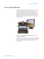

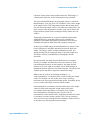

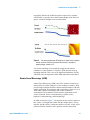
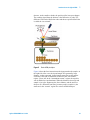
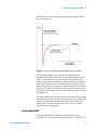


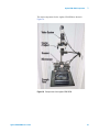
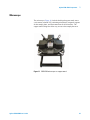
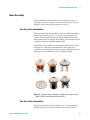


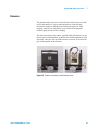


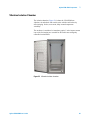

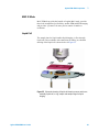


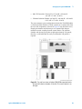
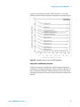


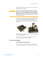
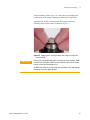


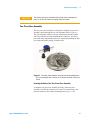
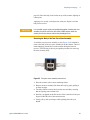
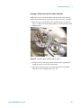
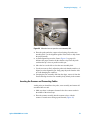
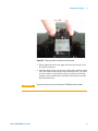
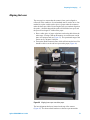
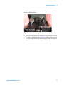


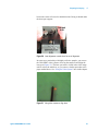
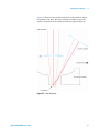
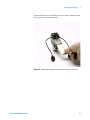


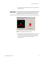
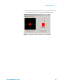

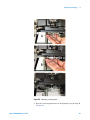

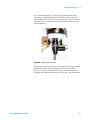


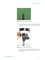
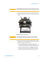
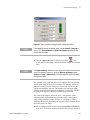
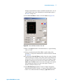
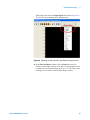


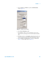


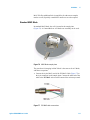
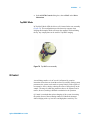
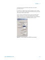
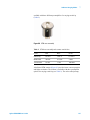


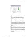
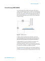


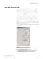


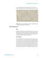
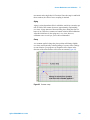
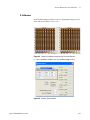

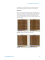


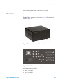

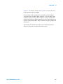

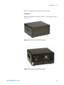
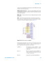


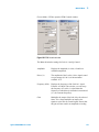


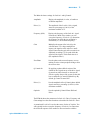

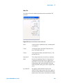


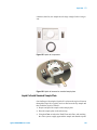

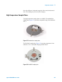

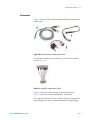

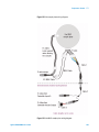


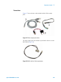
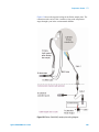
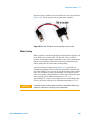
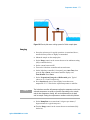
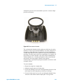

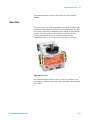

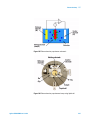
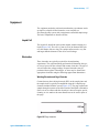


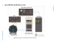
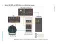
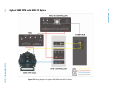
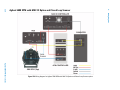


![Instalar y actualizar NetBSD-current [e] - Redes](http://vs1.manualzilla.com/store/data/006226705_1-100e74543fa3bea9f822ce307be8d1b9-150x150.png)