Download Multiple Depth DB Tables Indexing on the Sphere

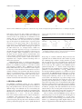
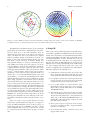
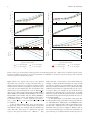
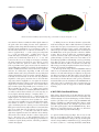
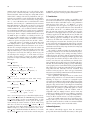
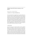
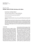
Hindawi Publishing Corporation
Advances in Astronomy
Volume 2010, Article ID 524534, 11 pages
doi:10.1155/2010/524534
Research Article
Multiple Depth DB Tables Indexing on the Sphere
Luciano Nicastro1 and Giorgio Calderone2
1 Istituto
2 Istituto
Nazionale di Astrofisica, IASF Bologna, Via P. Gobetti 101, 40129 Bologna, Italy
Nazionale di Astrofisica, IASF Palermo, Via U. La Malfa 153, 90146 Palermo, Italy
Correspondence should be addressed to Luciano Nicastro, [email protected]
Received 30 June 2009; Revised 13 October 2009; Accepted 12 January 2010
Academic Editor: Joshua S. Bloom
Copyright © 2010 L. Nicastro and G. Calderone. This is an open access article distributed under the Creative Commons
Attribution License, which permits unrestricted use, distribution, and reproduction in any medium, provided the original work is
properly cited.
Any project dealing with large astronomical datasets should consider the use of a relational database server (RDBS). Queries
requiring quick selections on sky regions, objects cross-matching and other high-level data investigations involving sky coordinates
could be unfeasible if tables are missing an effective indexing scheme. In this paper we present the Dynamic Index Facility (DIF)
software package. By using the HTM and HEALPix sky pixelization schema, it allows a very efficient indexing and management
of spherical data stored into MySQL tables. Any table hosting spherical coordinates can be automatically managed by DIF using
any number of sky resolutions at the same time. DIF comprises a set of facilities among which SQL callable functions to perform
queries on circular and rectangular regions. Moreover, by removing the limitations and difficulties of 2-d data indexing, DIF allows
the full exploitation of the RDBS capabilities. Performance tests on Giga-entries tables are reported together with some practical
usage of the package.
1. Introduction
Astronomical projects need to manage data which are
directly or indirectly related to sky coordinates. As larger and
larger datasets are collected by detectors at all wavelengths, it
is more and more crucial to efficiently manage those data to
speed up and optimize their exploitation. Modern database
servers (RDBS), being highly optimized for managing large
amounts of data, are the best available choice for today’s
astronomical project. The SQL language used to access
the data provides several high-level functionalities; still it
could be not enough since some scientific, in particular,
Astronomy specific capabilities and tools are missing. Speed
and flexibility of a query are strongly dependent on the
indexing used for the underlying DB table(s). Even simple
and in principle little resource-demanding tasks can become
highly inefficient if performed on poorly indexed archives.
Typically DB servers offer efficient indexing of one or more
1-d data using the so-called B-tree structure. However data
produced by an astronomical experiment are typically related
to sky coordinates which span a 2-d space. Although it is
possible to index such data using one or two simultaneous
1-d indexes like RA and Dec, the queries performance will be
very poor since the search criteria on a 2-d space can be much
more complex than on a union of two independent 1-d space.
Indeed the only possible queries that take advantages of such
indexes will involve range checking along the two coordinates
like α1 ≤ α ≤ α2 and δ1 ≤ δ ≤ δ2 . In some cases, the RDBS
provides built-in capabilities to manage 2-d coordinates into
index files using the R-tree structure. This would allow search
criteria like “Find all objects within 2 arcsec of a given
location.” However these functionalities are far from being
a standardized feature of RDBS; furthermore, there is room
for optimization and specialization for astronomical usage.
Fast data access is, for example, required by tasks like
cross-matching between two full-sky optical or IR catalogs.
Another example is the automatic fast astrometry of a field
aimed at quickly identifying transient sources, for example,
gamma-ray bursts optical transients. This is a typical task
of robotic telescopes. The transient source coordinates can
then be automatically communicated to larger instruments
in order to perform a more detailed study through spectral
or polarimetric observations. One more example is the quick
production of the map of a sky region showing some physical
or statistical property of the underlying DB entries. This
should be possible by using a simple, SQL standard query.
2
Web-based tools managing large-area surveys would greatly
benefit from fast RDBS response time too.
Luckily, like the amount of data, also DB servers
power and flexibility increase with time making possible
to dream, actually to start thinking about a DB table
with sub-arcsec sky resolution, that is, comparable to a
CCD pixel. We will see that DIF is just ready for this!
Building a Stellarium-like (http://www.stellarium.org/) or
GoogleSky-like (http://www.google.com/sky/) tool to browse
an astronomical data archive would then be the natural choice, with the obvious difference being that the
user can retrieve or work interactively with scientifically
meaningful data. Discussing the technical and financial
problems of such an ambitious project is beyond the
scope of this paper. We only mention the ESO VirGO
project (http://archive.eso.org/cms/virgo/) as a possible initial pathfinder.
The open-source package DIF (Dynamic Indexing Facility) [1] is a combination of a C++ library, a Perl script,
and SQL stored procedures allowing the automatic indexing
of MySQL tables hosting sky coordinates. The approach
adopted was to “discretize” a 2-d space and map it onto 1d space using a pixelization scheme. Each pixel is then tagged
with a unique integer ID so that an index can be created
using the standard B-tree. The usage of MySQL was a natural
choice as it was the only open-source RDBS which allowed us
to add a custom “DB engine” to the server. At the moment it
remains the only RDBS supported by DIF.
2. DIF Motivation and Architecture
The motivations for an efficient management of DB tables
hosting data with spherical coordinates are not different from
those of any other type of data. Exploiting large datasets
and performing complex types of queries are unfeasible, in
a reasonable amount of time, without an effective indexing.
Typically indexes are not just used to quickly select entries
within a given table, but also to define a “relation” with the
content of other tables in the DB. The capability to perform
“joined” queries is a key feature of relational databases. As
mentioned, indexing 2-d data (in order to allow spatial
queries) is quite different from the 1-d case because any
“sequential” data ordering, for example, along one direction,
inevitably causes data close in space to be distant in a table,
or disk file. Consider, for example, a catalog of objects;
in this case one can slice the sphere along the declination
(latitude) axis and sort in right ascension (longitude) within
each strip. Objects in each strip can be stored into a separate
table. Let us now assume that, upon a user request, a
dedicated task exists which identifies the stripes of interest.
If only one strip is affected by the query, then, depending
on how many objects are stored in that table/file, the task
of identifying and delivering the requested data is relatively
easy. In the case that several strips are to be searched, the
task will simply access and search all the affected tables. Of
course if the slicing is also performed along the RA axis,
the amount of data per table reduces, as does the response
time of such task. Moreover, instead of this geographic-like
grid, one can adopt any kind of sky slicing and manage
Advances in Astronomy
the requests accordingly. All this would work fairly well for
a cone-search service. Actually this method is adopted by
several catalog search tools (e.g., the VizieR service, vizier.ustrasbg.fr) with acceptable performance. Of course the search
efficiency depends on the relative size of the queried region
with respect to that of the slice. The closer the better. Also the
average number of objects falling into a slice must be not too
small nor too large. For example, the 1 billion objects USNOB1.0 catalog uses strips of 0.◦ 1 in declination, which means
that an average of half-million objects is present in each strip.
But what about importing those tables into a RDBS to
exploit its capabilities? For example, the usage of an RDBS
would allow to easily perform spatial joins on various catalogs. Not to mention the fact that a standard language (SQL)
is used to perform queries. This offers an infinitely greater
flexibility compared to a custom program which performs
a limited number of tasks, only works on a given catalog,
requires maintenance, and probably has little portability. As
already been said, once the data have been inserted into a DB,
one has to find an efficient indexing method for 2-d data.
A simple 1-d indexing on declination could be investigated
in order to estimate the RDBS performance with respect
to the previous custom management. We have not done
so and we do not expect a significant leap in performance
when compared to the custom case. In particular the RDBS
optimizer would be unable to take advantage of the index to
perform spatial joins. However other advantages of using an
RDBS remain.
The next step is then to find a method to cover the
sphere with cells (pixels) and number them. The resulting
set of integers can then be indexed using the conventional Btree and therefore the whole potential of the RDBS can be
exploited. So what we need is a 2-d to 1-d mapping function:
each entry in the table will have one single integer ID and a
sky area maps to a set of integers. A further step is identifying
the most appropriate pixel size. Likely this is project dependent, but we will see that having some thousands entries per
pixel could be a good choice. Among the various available
functions, those implemented by the Hierarchical Triangular
Mesh (HTM) [2] and the Hierarchical Equal Area isoLatitude
Pixelization (HEALPix) [3] tessellation schema are the most
suitable to our aim for a number of reasons; for example,
(1) they cover the sky uniformly with no singularities at
the poles, (2) the algorithm to compute the pixel IDs is
very fast, (3) they implement, or allow to easily implement,
tasks to work with the pixel IDs, (4) they are commonly
used in Astronomy, and (5) they are available as opensource C++ libraries (see http://www.sdss.jhu.edu/htm/ and
http://healpix.jpl.nasa.gov/). See Section 3 for more details.
The DIF core is represented by a MySQL DB engine
implemented into a C++ class. Functions to perform region
selection (and other tasks) use the HTM and HEALPix
libraries to calculate the IDs of the pixels included or touched
by the requested region. From the user point of view a
dynamic table is generated which contains only the entries
falling in the region. A DIF-managed table can be queried
as any DB table with the additional possibility to perform
queries on circular and rectangular sky regions, and so forth
(see below). In other words DIF extends the SQL language
Advances in Astronomy
3
cos (θ)
1
12
0, 0
0
−1
0
1
Azimuth/π
0, 180
1
2
(b)
(a)
Figure 1: The 12 HEALPix base pixels color coded for the “ring” scheme. Overplotted the pixel boundaries for k = 1 which gives 48 pixels.
and removes the need to write complex procedures or to
use temporary tables to perform 2-d selections. Notably, the
current version of the package has no limitations on the
number and type of simultaneous pixelizations applicable
to a table and the user can choose between two possible
types of select queries on spatial regions: (1) give the region
of interest in each query string, and (2) first define the
region of interest, eventually selecting a specific pixelization
depth, then perform any number and type of query on
the DIF created view (see examples below). Which one
is more convenient depends on the type of interaction of
the DB client application and complexity of the query one
needs to perform. What is important to note is that in
the latter case the selected region is retained until a new
region selection command is issued or the region selection
is cleared. This property could be useful in the future to
implement more complex selections involving union or
intersection of regions.
Additionally DIF offers (a) useful User-Defined Functions (UDFs) mainly derived from the HTM and HEALPix
libraries, (b) standalone programs to create fake test tables
with spherical coordinates, and (c) HEALPix-specific IDL
library which allows the user to obtain the result of a query
as a sky map. So who should use it? Potential users are those
wishing to manage in an automatic and effective way large
datasets of astronomical data, of whichever kind: objects
catalogs, observation logs, photon lists collected by spacebased high-energy detectors, single pixel counts of lowmedium resolution wide-field cameras, and so forth.
3. HEALPix and HTM
The HEALPix pixelization scheme [3] uses equal-area
pseudo-square pixels, particularly suitable for the analysis of
large-scale spatial structures. The base pixels are 12 with two
different shapes: four identical ones are centered along the
equator at 90◦ step starting from (0, 0); the remaining eight,
all identical, are centered at 45◦ longitude offset and at a fixed
poles distance of z ≡ cos θ = ±2/3 (θ is the colatitude),
four in the northern and four in the southern hemispheres
(see Figure 1). The region in the range −2/3 < z < 2/3 is
referred to as the equatorial zone, with the two remaining
regions being the polar caps. Recursive subdivision of these
pixels is performed keeping their centers equally distributed
Table 1: Relevant parameters for the HTM and HEALPix sphere
pixelization.
†
Npix
:
HTM
HEALPix
8 × 4d
2
12 × Nside
(where Nside = 2k )
ID range:
[Npix , 2 × Npix − 1]
[0, Npix − 1]
Max Npix :
9.0 × 1015
3.5 × 1018
Max res.∗ ( ):
1 × 10−2
4 × 10−4
2
(Ωpix = π/(3 × Nside
))
†d
(depth): [0, 25]; k (order⇔resolution parameter): [0, 29]
For HTM the maximum resolution is derived from the trixel minimum
side, for HEALPix assuming a square-pixel equivalent area.
∗
along rings of constant colatitude. Rings located in the
equatorial zone are divided into the same number of pixels,
the remaining rings contain a varying number of pixels.
The two rings closest to the poles always have 4 pixels and
going toward the equator the number of pixels increases by
four at each step. The resolution of the HEALPix grid is
parameterized by Nside = 2k , where k assumes integer values
being 0 for the base pixelization. It is called the “resolution
2
. Table 1 shows
parameter” or order. It is then Npix = 12×Nside
the relevant pixelization parameters (see Górski et al. [3] for
more details). The HEALPix library implements a recursive
quad-tree pixel subdivision which is naturally nested. The
resulting pixel numbering scheme is then referred as the
nested scheme. Alternatively the ring scheme simply counts
the pixels moving down from the north pole to the south
pole along each isoLatitude ring (see Figures 1 and 2). The
usage of the ring scheme is not recommended to index tables
like objects catalogs which are typically queried on small sky
regions. In fact in this case a data sorting will not result into
an efficient “grouping” like that obtainable for the nested
scheme where to “close-on-sky” pixels correspond “close-ondisk” data. This is important because data seek time is the
main issue to face when very large tables are considered.
The C++ library released in HEALPix version 2.10 uses
64-bit long integers to store the pixels IDs. This allowed us to
push the resolution of the pixelization to 4 × 10−4 arcsec.
However, because of 64-bit floating point arithmetics limitations (e.g., minimum appreciable angular distance), this
limit is not applicable for all the DIF implemented functions.
4
Advances in Astronomy
767
0
2
1
43
0
(a)
(b)
Figure 2: (a) The 8 HTM base pixels and recursive subdivisions on Earth surface. The “depth” d of the trixels is marked. (b) HEALPix
tessellation at order k = 3 giving 768 pixels whose colors encode their actual IDs in the “ring” scheme.
The HTM sphere pixelization scheme [2] uses triangular
pixels which can recursively be subdivided into four pixels.
The base pixels are 8, 4 for each hemisphere. They are
obtained by the intersection on the sphere of 3 major big
circles. On Earth they can be represented by the equator
and two meridians passing at longitudes 0◦ and 90◦ (see
Figure 2). These base spherical triangles all have the same
area. Each of them can then be further divided into
four spherical triangles, or trixels, by connecting the three
sides middle points using great circle segments. As can be
seen from Figure 2, from the first subdivision onward the
resulting trixels are no longer equal area. The scatter of the
trixels area remains within the ±70% of the mean area, which
is 2π/4d+1 , with d being the depth or level (step of recursive
subdivision) of the trixel. For a given depth the number of
trixels is Npix = 8 × 4d . The minimal side length is π/2d+1 and
the maximal is π/2 times the minimal length. The HTM
indexing algorithm performs recursive subdivisions on a unit
sphere using a quad-tree nested scheme and can identify
each trixel both by integer and string IDs which refer to the
vertices of the parent trixel counted counterclockwise (see
Kunszt et al. [4] for more details). This algorithm has proven
to be very efficient for selecting point sources in catalogs and
was specifically developed for the Sloan Digital Sky Survey
(see http://www.sdss.jhu.edu/ and [5]). Table 1 shows the
relevant pixelization parameters. Note that, similarly to the
HEALPix case, the depth 25 limit is imposed by the 64-bit
floating point calculations. It can be lifted up to 30 if 128bit variables and functions will be introduced in the source
code.
Unless one needs to access a large fraction of a table
and perform spatial analysis and map plot, we suggest to
prefer the HTM pixelization because it offers a larger set
of functions with respect to HEALPix. We will see below
that the HEALPix IDs of any set of selected rows can still
be computed using the DIF functions at query execution
time.
4. Using DIF
Here we give a brief technical description of the DIF components and its capabilities. Installation instructions and other
details can be found in the user manual distributed with the
package and available at the MCS( My Customizable Server,
ross.iasfbo.inaf.it/MCS/) website. The DIF source code can
be downloaded from the same place as a compressed tar
file. Note that being the DIF DB engine an extension to the
MySQL server, it requires that MySQL was/is installed using
the source package and that the path to the source code
location is supplied in the configuration step. DIF adds the
following components to a MySQL server:
(1) A DIF database with the two tables: dif and tbl. The
first is a dynamic table listing pixel IDs; the second
retains all the information about the managed tables.
(2) A set of SQL stored functions useful to get information
from the tbl table. Users can use them as an example
to implement their own functions/procedures.
(3) A set of SQL callable C++ utility functions usable
independently from the table type or query executed.
Most of these external UDFs make use of the HTM
and HEALPix libraries.
(4) The DIF DB engine, which feeds the DIF.dif table,
and a set of DIF specific sky region selection functions.
They are the compound of a C++ class plus functions
which rely on the HTM and HEALPix libraries to
dynamically, and transparently, compute the pixel
IDs of the region of interest.
(5) The dif Perl script used to perform various management tasks. It requires the DBD::mysql Perl library
to work (see Section 4.1).
(6) For each DIF indexed table. a number of views and
triggers will be created.
Advances in Astronomy
5
Note that DIF.dif is a table whose content is dynamically
generated by the DIF DB engine each time it is accessed,
transparently to the user, based on query search criteria. A
simple “SELECT ∗ from DIF.dif” without the usage of
one of the DIF specific sky region/pixels selection functions
will result in an “Empty set.” The DIF.tbl table hosts
all the necessary information about the DIF-managed tables,
like pixelization schema, depth/order, and name of the fields
with the coordinates. However, the only DIF components a
user needs to know about are two: (1) the dif script (for
a DB administrator) and (2) the DIF functions accessible
within MySQL queries. They are listed in Table 2. A detailed
description is reported in the user manual.
of all the available depths simultaneously by performing a
recursive “erosion” of the requested region. Let us say that we
have three indexes, 8, 10, and 12, then the algorithm will find,
in this order, that (1) the d = 8 trixels fully contained in the
region, (2) the d = 10 fully contained trixels in the remaining
area, and (3) the d = 12 fully and partially contained trixels
in what is left of the region. It could happen that no d = 8
or/and d = 10 trixel is found.
Sometimes it could be convenient to use only one of these
pixelizations, for example, when the queried region size is
close to the trixel size of one of the available depths. In this
case the user can issue the command
4.1. The dif Script. As mentioned, this section is of interest
only for a DB administrator. All the various actions related to
the management of a table via the DIF package are performed
using a Perl script: dif. Its parameters and flags can be
viewed typing dif --help. Its usage is straightforward and
we give here a partial list of examples.
Let us assume that a DB MyDB with a table MyTab exists,
that the sky coordinates of the entries are reported as centarcsec, and that the field names are RAcs and DECcs. To
index the table with an HTM tessellation with depth = 8, the
command to give is
which will create views like MyDB.MyTab htm 8 suitable to
directly perform queries using one single pixelization depth.
Of course this makes sense only if more than one pixelization
was applied (see below how to perform sky regions SELECT
queries on these views). To use a HEALPix tessellation with
“nested” scheme, k = 8, the command would have been
dif --index-htm MyDB MyTab 8
"RAcs/3.6e5" "DECcs/3.6e5",
and the result will be the following
(1) a column named htmID 8 of type MEDIUMINT
UNSIGNED (3 bytes) and default value 0 will be added
to the MyTab table,
(2) the column will be filled with the IDs of the trixel
where that entry falls,
(3) an index is created on the htmID 8 column,
(4) a new entry is inserted into the table DIF.tbl with
the values:
MyDB MyTab 1 0 8 RAcs/3.6e5 DECcs/3.6e5,
(5) a view named MyDB.MyTab htm is created. It contains the appropriate INNER JOIN of the htmID 8
column with the dynamically populated column
DIF.dif.id plus other statements (see the manual),
(6) a trigger named MyDB.difi MyTab is created. It is
used to automatically calculate the htmID 8 value
when an INSERT query is executed.
Moreover, if two or more pixelization depths are to be
applied to the table, they can be given simultaneously as a
comma-separated string. For example, to apply depths 8 and
12, the command would have been
dif --index-htm MyDB MyTab "8,12"
"RAcs/3.6e5" "DECcs/3.6e5".
A spatial query on the MyTab htm view performed via
DIF HTMCircle or DIF HTMRect/HTMRectV will make use
dif --single-index-views MyDB MyTab
dif --index-healpix-nested MyDB MyTab 8
"RAcs/3.6e5" "DECcs/3.6e5".
The added column name will now be healpID 1 8
(healpID 0 8 if the “ring” scheme was used) and the view
will be MyTab healp nest. To remove an index and the
related DIF facilities from a table, use a command like this
the following:
dif --drop-index-htm MyDB MyTab 8
which refers to the first of the two examples above. If one
wishes just to remove all the views and triggers from a
table but keeping indexes and columns created with a dif
command, then simply he/she can use dif --drop-views
MyDB MyTab.
4.2. UDFs: SQL Routines and SQL Callable C++ Utilities.
SQL stored functions are linked to the DIF database and give
access to the information stored in the DIF.tbl table. They
are usable in any query and are accessible to all MySQL users.
For example, to find out which are the table columns used to
get sky coordinates (in degrees!), one can execute the query
SELECT DIF.getRa("MyDB","MyTab"),
DIF.getDec("MyDB","MyTab");
SQL callable functions are MySQL “external” function; still
they can be used in any SELECT statement exactly like any DB
server built-in function. Apart from the spherical distance
calculation performed by Sphedist, they make available to
the user HTM and HEALPix related functions. Note that
the parameters “RA” and “Dec” are constants or the table
column names corresponding to spherical coordinates. As
mentioned, they must be in degrees; therefore conversion factors can be present, for example, RAcs/3.6e5. For example,
to get the HTM IDs at d = 6 of the neighbors of the pixel
where the point (100◦ , −20◦ ) falls, the command "select
6
Advances in Astronomy
Table 2: DIF functions available in MySQL.
SQL stored routines
DIF.getHTMDepth (db, tab)
DIF.getHEALPOrder (db, tab)
DIF.getHEALPNested (db, tab, k)
DIF.getRa (db, tab)
DIF.getDec (db, tab)
Sky region/pixels selection
DIF HTMCircle (Ra, Dec, r)
DIF HTMRect (Ra, Dec, S1, [S2])
DIF HTMRectV (Ra1, Dec1, Ra2, Dec2)
DIF HEALPCircle (Ra, Dec, r)
DIF HTMNeighbC (Ra, Dec)
DIF HEALPNeighbC (Ra, Dec)
DIF setHTMDepth (d)
DIF setHEALPOrder (s, k)
DIF Sphedist(Ra1,Dec1,Ra2,Dec2)
DIF FineSearch (var )
SQL callable C++ utilities
HTMLookup (d, Ra, Dec)
HEALPLookup (s, k, Ra, Dec)
HTMBary (d, ID)
HTMBaryC (d, Ra, Dec)
HTMBaryDist (d, ID, Ra, Dec)
HTMNeighb (d, ID)
HTMNeighbC (d, Ra, Dec)
HEALPBary (s, k, ID)
HEALPBaryC (s, k, Ra, Dec)
HEALPBaryDist (s, k, ID, Ra, Dec)
HEALPNeighb (s, k, ID)
HEALPNeighbC (s, k, Ra, Dec)
Sphedist (Ra1, Dec1, Ra2, Dec2)
Auxiliary functions
DIF useParam (d or k)
DIF cpuTime ()
DIF clear ()
Note: in DIF HTMRect if S2 is omitted it is assumed = S1, that is, query a square; s is the HEALPix schema switch: 0 for ring, 1 for nested.
HTMNeighbC(6, 100, -20)" will return the string:
37810, 37780, 37781, 37783, 37786, 37788,
37808, 37809, 37811, 37817, 37821, 37822,
37823.
The first of the 13 IDs is always the one containing the input
coordinates. Similarly to get the IDs of the neighbors starting
from a given pixel ID, use “selectHTMNeighb(6, 37810),”
which gives the same string above excluding the first ID, that
is, 12 IDs. Note that for HEALPix the number of neighbors
is not constant! More utility functions will be added in the
future.
4.3. The DIF Specific Region/Pixels Selection Functions. These
functions are those that allow the user to select the desired
subset of table rows making a (transparent) use of the
columns with the HTM and HEALPix IDs. They must be
used either in the query WHERE clause or as the only argument
of a SELECT statement to initialize the DB engine (see
below). The pixel neighbors and region selection functions
(the DIF HTM. . . and DIF HEALP. . ., see Table 2) only give
results if applied to the corresponding HTM or HEALPix
views as they produce a list of IDs in the dynamic table
DIF.dif, which is then used as a reference table to join the
managed table. For these functions, “RA” and “Dec” are the
table column names corresponding to the sky coordinates.
Also in this case, to have them in degrees, conversion factors
can be present. Note how these functions do not require
the pixelization parameters as they are directly managed by
the views they apply to. For example, DIF HEALPNeighbC
only requires the coordinates column names, compared to
the UDF HEALPNeighbC which also requires scheme ID and
order k. This dynamic management of the table is a specific
capability of the DIF DB engine. Some query examples with
direct region selection are
SELECT ∗ FROM MyTab htm WHERE
DIF HTMCircle(33,44,30);
SELECT ∗ FROM MyTab healp nest WHERE
DIF HEALPCircle(33,44,30);
SELECT ∗ FROM MyTab htm 8 WHERE
DIF HTMRect(33,44,40);
The first two queries return all the entries in a circular region
centered at α = 33◦ and δ = 44◦ with radius 30 . The third
will select entries in a pseudo-square region with same center
and sides length of 40 along RA and Dec.
Alternatively one can initialize the region of interest once
and then execute any number of queries on the resulting
entries. If multiple indexing has been applied (either HTM
or HEALPix), then one can also choose to use only one
depth/order, for example, d, k = 8. In this case the function
DIF useParam must be used. A typical sequence of queries,
for example, on an optical sources catalog, is:
SELECT DIF useParam(8);
SELECT DIF HTMCircle(5,3,60);
SELECT COUNT(∗) AS Nobj, AVG(B-V) AS
Clr FROM MyTab htm;
SELECT HEALPLookup(0,8,
RAcs/3.6e5,DECcs/3.6e5) FROM
MyTab htm;
The first two SELECT just set DIF internal parameters
returning 1 on success. The next query shows number and
Advances in Astronomy
average “color” of the sources within 1◦ around α = 5◦ , δ =
3◦ . The last query will calculate and return the HEALPix IDs
(order 8, ring scheme) of these sources. Note that cent-arcsec
coordinates are assumed. Omitting to use DIF useParam
or giving it the value 0 would instruct DIF to use all the
available depths (or orders) to perform the selection. This
is the default. Also note that the region selection query
can be followed by any number of queries on any table
view. Only the rows falling into the selected region will
be affected by these queries until a new region selection
command is issued. A DIF clear() can be issued to reset all
the internal parameters. The MySQL server is a multithread
process which means that it creates a new work environment
for each client connection. DIF functions, being part of the
server, set thread-specific parameters like any other MySQL
intrinsic function. Their status and values are retained until
the connection is closed. When a new connection with the
server is established, the initial status of a DIF parameter is
unpredictable (like the value of an uninitialized variable in a
program).
An example which makes use of all the three described
functions types is:
SELECT DIF.getRa("MyDB","MyTab") as
RAdeg,
DIF.getDec("MyDB","MyTab") as
DECdeg,
HTMNeighbC(6, RAdeg, DECdeg)
FROM MyDB.MyTab htm 6 WHERE
DIF HTMCircle(10,20,5);
The result will be the list of neighbors for each object ID in
the given circular region. Of course if more than one object
falls in one pixel, the output will present several identical
rows. It is trivial to modify the query to avoid this.
What about alternatives to DIF and in particular to the
DIF DB engine and related UDFs? One could, for example,
write a stored procedure which performs a cone search. First
of all the table must have been created with a column suitable
to receive, for example, HTM IDs at a given depth. For a
given cone, one needs to write a function to calculate the
IDs of the fully and partially covered trixels, then search the
table for all the entries with these IDs excluding those falling
outside the cone. The usage of a temporary table to store the
IDs is unavoidable. This could pose efficiency problems but
it is affordable. The usage of views and/or tables join would
certainly help. Additionally one has to manually manage the
insertion of new entries to calculate their IDs. The usage
of triggers could help. We can continue with the reasoning
requiring further facilities and tools and we will likely end
up with a system with an architecture which resembles the
DIF one, but is lacking the efficiency and flexibility intrinsic
to DIF.
5. Benchmarks
In order to perform benchmarks on access time of DIFmanaged tables, we used several tables with fake entries.
Some of them were produced generating fully random
7
Table 3: Parameters for the HTM and HEALPix pixelization used
in the tests.
d/k
Npix
Rows/Pix.
Bytes∗
1.26†
283
18
89,290
5,580
348
2
3
3
1
21
4
<Area>
(arcmin2 )
HTM
6
8
10
32,768
524,288
8,388,608
12
134,217,728
HEALPix
6
49,152
0.84†
59,526
2
8
10
12
786,432
12,582,912
201,326,592
189
12
0.7
3,720
232
14
3
3
4
† (deg2 ); ∗ additional
disk storage per row needed.
coordinates; this means that the sky distance between two
sequentially generated entries could be anything in the range
[0◦ , 360◦ [. It also means that a set of “close-on-sky” entries
could be spread all over the disk data file. Other tables had
their entries generated following a ∼ 1◦ sky pixelization
schema. This means that the data spread within the disk files
is reduced by a factor equal to the number of pixels used
to split the sky. For simplicity and analogy with the GSC
2.3 catalog (see below) we generated the entries over 32768
pixels corresponding to the HTM of depth 6 grid. Tables with
average objects/pixel density in the range ∼ 10000–90000
were produced (i.e., containing 0.4–3 billion entries). We
also produced and performed tests on “pixelized” and
RA sorted (within each pixel) table. The 3 billion entries
tables gave disk files size of ∼ 120 GBytes. All the tables
were created using the MyISAM DB engine. We avoided to
split tables, and then the data files, by using the MERGE
DB engine or the PARTITION BY option as, apart from
management convenience, we do not expect any significant
performance improvement on machines not equipped with
a large number of disks. Region selections were performed
using coordinates in degrees and cent-arcsec. Because the
HEALPix library does not allow rectangular selections, for
homogeneity reasons the selections were only performed on
circular regions (also referred to as “disc” or “cone”). Four
different pixelization depths/orders were used both for HTM
and HEALPix (nested scheme) and the queries involved
only one of them at the time. The results of benchmarks
using the multidepth facility on very large tables will be
reported elsewhere. The relevant parameters are reported in
Table 3. We used a custom program to monitor the system
resources usage by the select queries on DIF-managed tables.
As expected, the most important hardware component
determining the overall query execution time is the hard
disk, in particular its data seek and access time. The higher
the data contiguity the faster the query execution time.
The used query implied calculations on the rows content;
this is in order to force the load of the data into memory
and not to have just a row counting. For each pixelization
8
Advances in Astronomy
100
Elap. time (s)
10
1
105
105
104
103
104
103
102
101
105
104
104
N (pixels)
105
103
102
101
103
102
101
100
100
100
100
NPpart /
NPtot (%)
N (pixels)
1
0.1
102
101
NPpart /
NPtot (%)
10
0.1
Nrows (s−1 )
Nrows (s−1 )
Elap. time (s)
100
10
1
1
10
Query disc radius (arcmin)
d = 6 (89290 objs/pix)
d = 8 (5580 objs/pix)
100
d = 10 (348 objs/pix)
d = 12 (21 objs/pix)
(a)
10
1
1
10
Query disc radius (arcmin)
k = 6 (59526 objs/pix)
k = 8 (3720 objs/pix)
100
k = 10 (232 objs/pix)
k = 12 (14 objs/pix)
(b)
Figure 3: Select query execution times and other parameters for a DIF-managed table with ∼3 billion entries as a function of the disc radius.
Results for four different pixel scales are reported both for HTM (a) and HEALPix (b). Each point represents the average of the results from
50 queries performed on random sky positions.
Figure 3 shows, in a log-log scale, respect to the queried
disc radius (top to bottom): (1) query execution times, (2)
number of processed rows per second, (3) number of pixels
involved, and (4) number of partially covered pixels respect
to the total at a given depth/order. The used machine main
characteristics are OS: Linux kernel 2.6.22.19 SMP x86 64,
CPU: bi-proc. dual-core Intel Xeon 5130 @ 2 GHz, RAM: 8
GBytes DDR2-667 166 MHz, and Disk: RAID 1 on a 3 Ware
Raid 9550SX-8 LP controller with two SATA2, 500 GBytes,
7200 rpm, 3 Gbits/s, reiserfs. The MySQL version used is
5.1.32 with key buffer = 384 M, myisam sort buffer
size = 64 M, query cache size=32M. The main results
are as follows.
(a) For the fully random tables, query execution times
are quite long because to fast index lookups corresponds
slow disk file seeking (not scanning) which could affect the
entire data table. Times grow in a quasi-linear way with
respect to the region size and it is of ∼ 100 rows s−1 . This
makes clear that, even though it is better than having, for
example, a simple declination indexing, the usage of DIF
on such sort of table is of very limited help. On the other
hand, any real data would almost never be produced in a fully
random way, but rather in a sequential way over sky “spots”
or “stripes”. This is, for example, the case of all-sky surveys
performed in point-and-stare or slewing mode. A possible
solution is to perform data clustering by sorting over the DIF
index with lower depth/order using myisamchk -R index (see
myisamchk manual).
(b) The HTM depth 6 sorted tables behave quite differently and show better performance when pixels with area
of ∼ 200–300 arcmin2 (HTM depth = 8 and HEALPix order
= 8) are used to index the tables. This is particularly true for
the table with ∼ 3 billion rows we used, where we have some
thousands entries per pixel (see Figure 3). Having a look to
the curves measuring query execution time and number of
processed rows per second as a function of the region size, we
Advances in Astronomy
9
(B − V )
1.1
Objects
800
0
(a)
0.4
(b)
Figure 4: UCAC 2.0 full sky objects density map (a) and ASCC 2.5 objects average B − V (b).
note that the behavior is similar for all the depths. However
the point where the bending becomes more significant is
depth dependent being shifted toward larger number of rows
for higher depth pixelizations. As a consequence of this, we
also note that, when some 1 × 105 rows are involved, d = 6
starts to perform like d = 8. The rows/s processing limit
is ∼ 5 × 105 . For tables with ∼ 1 billion rows or less we
found that higher resolution pixelizations (d, k = 10, 12)
perform not too differently from the d, k = 8 case. The
reasons for this are not so simple to investigate considering
the many parameters involved. We note that for a given
region size, when the pixel size reduces, the number of
joins on pixel IDs in the query increases but the number of
entries falling into partially covered pixels, for which a direct
distance calculation from the center of the circle is required,
decreases. It is likely that, depending on DB server and
machine characteristics, the performance can vary with pixel
density and number of join operations required. However,
as already been mentioned, we do not note any significant
dependence of the query execution time on the total CPU
usage time, which is negligible. So, once again, the attention
should fall on the data seek/access time and consequently its
impact for the various pixel densities. Let us assume that a
given circular region only partially covers 1 trixel at d = 8;
this is typically the case for a ∼ 1 radius region. In this
trixel entries coordinates are randomly distributed. However
we will access all of them on disk, so, in some way, they are
accessed quite efficiently having a “contiguity factor” fc =
1/16 (being the data clustered on d = 6 trixels and for each
depth step there is a factor four increase in the number of
trixels). It is not a constant, but let us say that at d = 10 the
very same region partially covers two subtrixels of that trixel.
The number of entries to seek/access reduces by a factor
eight. Considering that the various processes involved will
likely put in cache memory adjacent data, we can assume that
there is one single data seek operation to access these rows.
However now it is fc = 1/256, that is, the data are a factor
eight more fragmented. Now if we half the entries density,
the benefit of the reduced seek time is a factor eight greater
for d = 10 respect to d = 8. This explanation seems to us
sufficient to account for the measured query performance as
a function of pixel density and size; still other possibilities
could be investigated.
(c) Adding (in our case) the RAcs column to a given table
index and sorting the data on disk with this new combined
index reduce the query execution time by a variable, still not
very significant amount of time. On the other hand, time
reduces by up to an order of magnitude if one uses directly in
the WHERE clause of the query the RAcs column to delimit
a range. This is what we did in the customized catalogs
used for astrometry and objects matching in the REM [6]
produced images (see below). Moreover, if one makes use of
the buffering capabilities of the MySQL server by performing
more than one query on the same sky region, the queries
other than the first one will be executed in a very fast way.
This strategy can easily be implemented in robotic telescopes
software, for example, for GRB alerts!
(d) The usage of the “ring” scheme for HEALPix indexed
tables is not recommended because any table sorting which
makes use of such index will give for adjacent on sky pixels
not adjacent position on disk. This effect is less relevant in
the extreme cases when a few or the majority of the pixels are
interested by a selection. Because of the poorer performance
measured and because the calculation of the HEALPix IDs of
table entries can be computed at query execution time, for
a general purpose table we suggest to use always the HTM
indexing.
6. MCS-IDL Contributed Library
MCS offers a client interface to the IDL language. We have
implemented a library useful to interact in a very simple way
with the MySQL server from this language. A further library
useful to plot data on the sphere using the HEALPix IDL
library is available too. DIF-managed tables data are easily
plottable using this library. It is enough to put them on the
user’s IDL path together with the HEALPix library. These
libraries are retrievable from the web. Here we show their
usage on customized optical and IR catalogs.
6.1. Optical and IR Catalogs Sky Maps. For our tests on real
data we used catalogs which are routinely used for realtime objects identification in images taken by the IR/optical
robotic telescope REM (see Molinari et al. [6]). Among them
are GSC 2.3, GSC 2.2 (∼ 18th mag threshold), USNO B1.0,
10
Advances in Astronomy
2MASS, UCAC 2.0, and ASCC 2.5 (see the websites: wwwgsss.stsci.edu/, www.nofs.navy.mil/, www.ipac.caltech.edu/,
ad.usno.navy.mil/, cdsarc.u-strasbg.fr/). Using DIF, we have
indexed these catalogs with various pixelizations. The performed tests confirm the results obtained for the fake tables,
that is, the fastest access time is achieved by using pixels of
size ∼ 1◦ . We recall that the GSC 2.3 is distributed as 32768
FITS files, each covering a d = 6 HTM trixel, whereas USNO
B1.0 and 2MASS are split in files covering 0◦ .1 in Dec, RA
ordered in the slice. To further speed up the region lookup,
which for REM is 10 × 10 , we added coordinates indexing.
For optimization and disk space-saving reasons, coordinates
were converted into cent-arcsec and therefore packed into 4byte integers. Then a “unique” combined index was created
on HTM ID plus coordinates. As already noticed in [1],
with such an index and the usage of coordinate ranges in
the WHERE clause to further reduce the number of rows to
seek/access, queries on regions of size 10 –30 take ∼ 20 ms.
Using IDL routines to visualize as sky maps data read
from MySQL tables is quite straightforward. As said, the
HEALPix pixelization schema and routines can be used to
this aim. For example, in Figure 4 we show the UCAC 2.0
sky objects density in galactic orthographic projection. The
map was built using k = 8, that is, a pixel size of 14 . The
sky region not covered by the catalog is shown in grey. In
the same figure the average B − V of the ASCC 2.5 objects
in pixels of area 13.4 deg2 is shown in galactic mollview
projection. A simple (and basic) IDL program to produce the
first map is:
@mcs healplib
COMMON HEALPmap, $
hp nested, hp nside, hp order, $
hp npix, hp emptypix, hp npixok, $
hp map nocc, hp map sum
hp order = 8
Query = "select healpID 0 8 from UCAC 2orig"
DBExec Qry("MyDB name", "User name", $
"Password", Query)
healp MapFill()
orthview, hp map nocc, rot=[45,45], $
coord=["C","G"], /grat, col=5
Note: (1) mcs healplib(.pro) has all the high-level routines needed to build and save HEALPix maps; it also loads
mcs usrlib which is used to access MySQL tables. (2) The
common block HEALPmap is used to pass the map parameters among the various routines. (3) If the UCAC 2orig
table does not have the healpID 0 8 column (e.g., it is
not indexed), then simply change the query into "select
HEALPLookup(0,8, RAcs/3.6e5,DECcs/3.6e5) from
UCAC 2orig" which will calculate the IDs for k = 8 on the
fly. (4) healp MapSave() can be used to write the map into
an FITS file. On the MCS website some demo programs are
available to help write custom programs and routines.
7. Conclusions
We presented the DIF software package, its capabilities, and
the results of benchmarks over very large DB tables. We have
shown that for tables with billion entries a sky pixelization
with pixel size of the order of ∼ 15 (HTM d = 8) gives
best performance for select queries on regions of size up to
several degrees. At this spatial resolution some thousands of
entries fall in each of the ∼ 1/2 million pixels; these entries
have the same ID assigned in the DB table. We stress the
fact that these results apply only in case some sky coordinates
ordering is applied to the disk data file. If not, the disk seek
time becomes so dominant to make the use of DIF, or any
other indexing approach, meaningless. We also note that,
in all cases, the CPU time accounts for only a few percent
of the total query execution time; therefore great care must
be put in choosing and designing the data storage. We have
also shown the usage of HEALPix IDL libraries allowing the
visualization and saving of sky maps obtained executing SQL
queries directly from IDL.
The package is distributed under the GNU GPL and we
encourage everybody to use it for their astronomical projects,
in particular to manage object catalogs and large archives
of data of any sort. We believe that the Virtual Observatory
could certainly benefit by adopting a DIF-like approach and
we hope that VO software developers will consider it. It is
worth to note that not only Astronomy can benefit of the
usage of DIF. It can be used by any project dealing with spherical data. Research fields like geology, geodesy, climatology,
oceanography, and so forth all deal with geographical data.
Those data can be stored into a DB, indexed on coordinates
using DIF, and then efficiently retrieved, visualized, and
used for a variety of purposes. Some new type of automatic
navigation system having a DBS behind could also find more
convenient a DIF indexing approach.
More capabilities and improvements are under development among which are cross-match UDF for automatic
matching of objects in a circular or rectangular region
selected from two different tables and the full porting to Mac
OS. Other types of selection region, like regular and irregular
polygons, rings, and so forth, or the adoption of commonly
used region definition strings will be considered too. Though
widely tested, the package is periodically update to remove
bugs, improve performance, add new facilities, make it
compatible with new MySQL versions, and so forth. Any
comment or feedback is welcome. Users willing to contribute
to the package development or testing are kindly asked to
contact us. Please visit the website: ross.iasfbo.inaf.it/MCS/.
The now available DIF version 0.5.2 introduced some
changes with respect to the version used when writing this
paper. The reader is asked to read the user manual available
with the software package at the mentioned website.
Acknowledgments
The authors acknowledge support from the astrometry
group of the Turin Astronomical Observatory to have given
Advances in Astronomy
us access to the various optical and IR catalogs. DIF makes
use of the HEALPix [3] and HTM [2] packages. They also
thank the referee for his/her helpful comments.
References
[1] L. Nicastro and G. Calderone, “Indexing astronomical database
tables using HTM and HEALPix,” Astronomical Society of the
Pacific Conference Series, vol. 394, pp. 487–490, 2008, Edited by
R. W. Argyle, P. S. Bunclark, and J. R. Lewis.
[2] P. Z. Kunszt, A. S. Szalay, and A. R. Thakar, “The hierarchical triangular mesh,” in Proceedings of the MPA/ESO/MPE
Workshop—Mining the Sky, A. J. Banday, S. Zaroubi, and M.
Bartelmann, Eds., pp. 631–637, Springer, Garching, Germany,
2001.
[3] M. Górski, E. Hivon, A. J. Banday, et al., “HEALPix: a
framework for high-resolution discretization and fast analysis
of data distributed on the sphere,” The Astrophysical Journal,
vol. 622, no. 2, pp. 759–771, 2005.
[4] P. Z. Kunszt, A. S. Szalay, I. Csabai, and A. R. Thakar, “The
indexing of the SDSS science archive,” Astronomical Society of
the Pacific Conference Series, vol. 216, pp. 141–144, 2000, Edited
by N. Manset, C. Veillet, and D. Crabtree.
[5] J. Gray, A. S. Szalay, A. Thakar, et al., “Data mining the SDSS
SkyServer database,” in Proceedings of the 4th International
Workshop on Distributed Data and Structures (WDAS ’02), W.
Litwin and G. Levy, Eds., pp. 189–210, Carleton Scientific, Paris,
France, 2002.
[6] E. Molinari, S. Covino, S. D’Alessio, et al., “REM, automatic for
the people,” Advances in Astronomy. In press.
11
Hindawi Publishing Corporation
http://www.hindawi.com
The Scientific
World Journal
Journal of
Journal of
Gravity
Photonics
Volume 2014
Hindawi Publishing Corporation
http://www.hindawi.com
Volume 2014
Hindawi Publishing Corporation
http://www.hindawi.com
Volume 2014
Journal of
Advances in
Condensed Matter Physics
Soft Matter
Hindawi Publishing Corporation
http://www.hindawi.com
Volume 2014
Hindawi Publishing Corporation
http://www.hindawi.com
Volume 2014
Journal of
Aerodynamics
Journal of
Fluids
Hindawi Publishing Corporation
http://www.hindawi.com
Hindawi Publishing Corporation
http://www.hindawi.com
Volume 2014
Volume 2014
Submit your manuscripts at
http://www.hindawi.com
International Journal of
International Journal of
Optics
Statistical Mechanics
Hindawi Publishing Corporation
http://www.hindawi.com
Hindawi Publishing Corporation
http://www.hindawi.com
Volume 2014
Volume 2014
Journal of
Thermodynamics
Journal of
Computational Methods in Physics
Hindawi Publishing Corporation
http://www.hindawi.com
Volume 2014
Journal of
Hindawi Publishing Corporation
http://www.hindawi.com
Volume 2014
Journal of
Solid State Physics
Astrophysics
Hindawi Publishing Corporation
http://www.hindawi.com
Hindawi Publishing Corporation
http://www.hindawi.com
Volume 2014
Physics
Research International
Advances in
High Energy Physics
Hindawi Publishing Corporation
http://www.hindawi.com
Volume 2014
International Journal of
Superconductivity
Volume 2014
Hindawi Publishing Corporation
http://www.hindawi.com
Volume 2014
Hindawi Publishing Corporation
http://www.hindawi.com
Volume 2014
Hindawi Publishing Corporation
http://www.hindawi.com
Volume 2014
Journal of
Atomic and
Molecular Physics
Journal of
Biophysics
Hindawi Publishing Corporation
http://www.hindawi.com
Advances in
Astronomy
Volume 2014
Hindawi Publishing Corporation
http://www.hindawi.com
Volume 2014