1
6
BORDEV user manual
BORDEV is a modular, menu-driven computer program developed to solve
problems in the design, operation, and evaluation of sloping border irrigation
systems. You start the module BORDEV by selecting it in the SURDEV package. The installation procedure of this package was discussed in Chapter 4,
Section 1.
1
6.1
Menu structure
There are six main menu items, five of which have sub-menus that you can
select by moving the highlight with the arrow keys and pressing [Enter], or by
typing the red (bold) character. Table 6.1 shows the structure of the main
menu and its first layer of sub-menus.
6.1.1 Sub-menu files
The sub-menu Files gives you two options: Load and View /Print. With Load,
you can select an existing file and continue with the calculations. With
ViewlPrint you can select an existing file, the contents of which will subsequently be displayed on the screen. Pressing [F5] gives you the option of sending the contents of this file to a printer, a text file, or a spreadsheet file. For
more information on these topics, see Chapter 4,Section 4.3.
6.1.2 Sub-menu operation
In the sub-menu Operation, you can select the appropriate system operation
mode. If you select Fixed flow it means that a constant inlet flow rate will be
used to irrigate the borders during the entire application time. Selecting
Cutback flow means that, at the end of advance, the inflow is reduced for the
remainder of the application time. Selecting Tailwater reuse refers to a border
Table 6.1 Bordev menu structure
Files
Operation
Load
Fixed flow
ViewPrint Cutback flow
Tailwater reuse
Units
Infiltration
Calculation
Flow rate
Length
Depth
Time
Modified SCS families
1. Flow rate
Kostiakov-Lewis equation 2. Length
3. Cutoff time
4. Min. Depth
Quit
67
irrigation system with a runoff reuse arrangement. Because BORDEV only
simulates the flow in one border, the reuse component is not integrated in the
required flow rate of another border. The default operation mode is Fixed flow.
6.1.3 Sub-menu units
The sub-menu Units is where you can choose pre-determined units for flow
rate, length, depth and time. The following units are available:
- Flow rate: Litres per second, US gallons per minute, cubic metres per
minute, or cubic feet per minute.
- Length:
Metres or feet, used for border length and width.
- Depth:
Millimetres or inches, used for the various supplied and infiltrated depths.
- Time:
Minutes or hours, used not only for advance, cutoff, depletion
and recession time, but also for the infiltration equations.
The selected units are maintained throughout the program and are also saved
with the file. When the program is started, default units are: litres per second
for flow rate; metres for border dimensions; millimetres for infiltrated depths;
and minutes for time.
6.1.4 Sub-menu infiltration
In the sub-menu Infiltration, you can select one of two different infiltration
input modes. Both modes are based on the infiltration characteristics of a soil
as described by the Kostiakov-Lewis equation (Equation 3.4):
Di = kTA + foT
where Di is the cumulative infiltration after an infiltration opportunity time
T, k is the infiltration constant, A is the infiltration exponent, and f, is the
basic infiltration rate. In BORDEV, you can enter the soil infiltration characteristics A, k, and f, directly or indirectly by using the modified SCS families.
For more background information on this subject, see Chapter 3, Section 1.1.
The default infiltration input mode is the Modified SCS families.
6.1.5 Sub-menu calculation
Before actual data can be entered and calculations can be made, you have to
select one of the four modes in the sub-menu Calculation (Table 6.1). What the
first three modes have in common is that the calculated minimum infiltrated
68
depth at the downstream end of the border always equals the required depth.
In other words, no under-irrigation will occur at the downstream end, whereas over-irrigation always occurs in the upstream part. When to use the various modes is summarised below.
Calculation Mode 1: Flow rate
Calculation Mode 1is primarily for design purposes, when you know the border dimensions and want to know the approximate flow rate that is needed to
achieve a reasonable performance. The program will also give you the
required cutoff time and the primary performance indicators as well as various depth and time parameters.
For the operation modes Fixed flow and Tailwater reuse, BORDEV calculates the flow rate in such a way that the application efficiency is approximately maximised. For the operation mode Cutback flow, the flow rate is
determined so that the user-specified advance ratio is achieved. Although the
result obtained in this mode is usually close to these targets, it is nevertheless
required that you continue running in Modes 3 and/or 4, because in most
cases small refinements are still possible.
Calculation Mode 2: Dimensions
Calculation Mode 2 is the reverse of Calculation Mode 1:the flow rate is now
known and you want to know the approximate border dimensions that are
needed to achieve a reasonable performance. The program will also give you
the required cutoff time and the primary performance indicators as well as
various depth and time parameters. In this Mode, the user is required to give
the lengthlwidth ratio a figure. The maximum application efficiency is approximate and to get a final result you must continue in Modes 3 and/or 4.
Calculation Mode 3: Cutoff time
Calculation Mode 3 is one of the two main modes of BORDEV. It will be the
one most frequently used and will also be the starting mode for the experienced user. Here, both the flow rate and border dimensions are input. The
required cutoff time is the resulting design variable, while the application efficiency and other secondary output are also given. Note, in this mode, the
advance ratio is an output, because it is not possible to fix advance ratio, border dimensions and flow rate and, at the same time, satisfy the requirement
that the minimum infiltrated depth equals the required depth.
Calculation Mode 4: Minimum Depth
This is the other main mode of the program. The cutoff time, border dimensions and flow rate are specified as input. Thus, all design variables are input,
which means that the required depth at the end of the field will usually not be
achieved (ie, that under and/or over-irrigation can occur). The minimum infiltrated depth that occurs at the far end of the field is the main item that deter69
mines whether there is under or over-irrigation. It is therefore given as first
output, together with the primary performance indicators: application efficiency, storage efficiency and distribution uniformity. This mode is most suitable
for performance evaluation of an existing border irrigation system and for testing the performance sensitivity to a change in the field parameters.
6.2
Input windows
After you have selected a calculation mode, BORDEV will display the input
screen for data entry: Field Parameters and Input Decision Variables. The
input data to be provided in the two windows are summarised in Table 6.2.
6.2.1 Field parameters
Infiltration
Upon selection of the Modified SCS families type of infiltration data, BORDEV will use it for borders, as was discussed in Chapter 3, Section 1.1. One
of seventeen families can be chosen. If a wrong number is typed, an error message with a list of acceptable numbers is shown. To select a particular family,
you can use the Help screen by pressing [Fl] while the cursor is on the family number. A screen with the possible numbers will pop up from which you can
make your selection (Figure 6.1).
Table 6.2 Input variables for the Bordev calculation modes
Item
Field Parameters
Infiltration
Required depth
Flow resist.
Slope
Input Decision Variables
Inlet flow rate
Lengtwwidth ratio
Border length
Border width
~ k t o f time
f
Advance ratio
Cutback ratio
Tailwater recovery ratio
70
Fixed flow
Cutback flow
Tailwater reuse
Mode
Mode
Mode
1
2
3
4
1
O
0
0
0
O
O
0
0
0
O
O
0
0
0
O
O
0
0
0
O
O
0
0
O
O
2
3
4
1
0
0
o
o
O
0
0
0
0
o
O
0
0
0
0
0
o
O
0
0
0
0
0
o
O
0
0
0
0
o
O
0
O
2
3
O
4
0
O
O
O
0
O
O
0
O
O
0
O
O
0
O
O
0
O
O
0
0
0
O
O
O
0
O
0
0
o
O
0
erosion.is not a problem, except possibly at the head, where water velocity
depends on the way in which the total inflow is supplied to the field (pointinlet, type of inlet structure, head ditch, siphons).
6.2.2 Decision variables
Decision variables in surface irrigation are normally the field dimensions
(length and width), flow rate, and cutoff time. Which of these parameters
appear under the heading Input Decision Variables depends on the calculation
mode you have selected (see Table 6.2).
Border dimensions
In Modes 1 , 3 and 4 you can prescribe values for the border length and width.
For open-ended borders, an optimum length applies. A field that is too long
-will result in a low performance because of a long advance time, with consequently an uneven infiltration and high deep percolation losses. On the other
hand, a field that is too short would result in surface runoff that is too high.
Consequently, for open-end borders, the optimum length (with all other variables given) is where the sum of deep percolation and surface runoff losses is
at its minimum and hence the application efficiency is at its maximum.
Length 1width ratio
In Mode 2, the lengtwwidth ratio is required to allow the program to calculate
the border dimensions, based on a given flow rate.
Flow rate
In Modes 2, 3 and 4 you can assign values to the total flow rate available for
the field. In BORDEV, this inflow rate is divided by the field width to obtain a
unit flow rate per metre width, which is used in the numerical simulations.
The flow rate should not be too low, otherwise the flow would not reach the end
of the border. It should also not be too high, to avoid excessive runoff. Thus,
with open-end borders, there is an optimum flow rate (similar to the optimum
border length), whereby the sum of deep percolation losses and surface runoff
losses is at its minimum, meaning a maximum application efficiency.
Cutoff time
In Modes 1 , 2 and 3, the cutoff time is a result of the calculations. In Mode 4,
a user-specified value can be given. For all three irrigation methods, cutoff is
usually done some time after the end of advance, so that the required depth
can infiltrate at the downstream end. When the cutoff time is substantially
later than advance time, it will have a clear effect on recession, and thus on
deep percolation and surface runoff losses. When cutoff is too early, the
required depth at the end of the field may not be achieved.
72
Advance ratio
The advance ratio, defined as the ratio of advance time to cutoff time, is especially of interest in cutback operation, where it can be either input or output,
depending on the purpose (Mode) of the simulation.
Cutback ratio
The cutback ratio must be specified in all calculation modes during a cutback
operation. It is defined as the ratio of the reduced flow rate to the initial flow
rate, such that the reduced flow is sufficient to keep the entire field length
wetted as long as is necessary, while at the same time reducing the surface
runoff. Because of the calculation algorithm used, cutback is assumed to be
done when the water has reached the end of the field.
Tailwater reuse ratio
The tailwater reuse ratio must be specified in all calculation modes for a reuse
operation. It is defined as that part of the surface runoff that is reused and
applied directly to calculate the application efficiency. A ratio of 1 would be
ideal but may not always be possible, particularly because of high costs of the
reuse system.
6.2.3 Input ranges
Ranges have been fixed for all input variables as shown in Table 6.3 and are
in metric units. If other units are chosen in the menu, the indicated ranges
are converted in the program.
Table 6.3 Accepted ranges of input parameters
Input parameters
Field Parameters
Intake family #
Infiltration coefficient, k
Infiltration exponent, A
Infiltration constant, f,
Required depth, D,,
Flow resistance, n
Field slope
Input Decision Variables
Border length, L
Border width, W
Lengthlwidth ratio, LIW
Flow rate, Q
Cutback ratio
Advance ratio
Tailwater reuse ratio
Cutoff time, T,,
Accepted values
0.05 - 2.0
0.05 - 50 “/minA
0.01 - 0.8
0.005 - 30
33 - 250 mm
0.01 - 0.40
0.0005 - 0.05 m/m
50 - 500 m
1- 200 m
1 - 30
1- 250 US
0.65 - 1.00
0.1 - 0.9
0.1 - 1.0
10 - 2000 min
73
Based on a large number of runs, the ranges have been fixed in a bid to avoid
too many impossible combinations and corresponding error messages. For all
practical purposes, the ranges of the individual parameters will be more than
sufficient. If you combine extreme values of the individual parameters you may
not get a result. In that case, BORDEV will flash you a message on the screen
indicating how to change these values in order to get a result.
The above ranges are ignored for output results, so, no warning will be given
if such an out-of-range value is subsequently used as input in another mode.
6.3
Output Windows
When you have keyed in all the data, press [F2] for the calculations and the
output. The screen again shows the two input windows, but a third window
has now been added, showing the results (Figure 6.2). These results are presented in various groups, separated by a blank line. The first group contains
the desired variable or variables according to the calculation mode you have
selected: in Mode 1they are the flow rate and the cutoff time; in Mode 2 the
border length, the border width and the cutoff time; in Mode 3 the cutoff time;
and in Mode 4 the minimum infiltrated depth.
The second group contains the primary performance indicators as discussed
in Chapter 3, Section 3. All the calculation modes allow the performance of an
irrigation scenario to be evaluated with the application efficiency, surface
runoff ratio, deep percolation ratio, distribution uniformity and uniformity
coefficient; Mode 4 adds the storage efficiency. Finally, using [PgDnl, you
deq". depth
Flow resist.
0.15
-
Border l e n g t h =
Border w i d t h
150 m
20 m
OUTPUT, Fixed f l o w , Mode 3
c u t - o f f time
Figure 6.2
.74
Bordev output example
=
232 min
AppliC. e f f i c i e n c y =
surf. run-off r a t i o =
Deep perc. r a t i o
=
65 %
Distr. uniformity
unif. coefficient
=
84 %
=
94 %
23 %
13 %
obtain two groups with secondary output variables: times and depths.
Outputs in all calculation modes are advance time, depletion time, recession
time and intake opportunity time corresponding to the downstream point.
In all the calculation modes, BORDEV provides information on the maximum, minimum and average infiltrated amounts, together with the amount
of surface runoff. In addition, Mode 4 also presents the amount of overhnderirrigation as the average amount over that part of the border that received
deficit/excess irrigation. The output also includes the length of the border
segment over which deficit and/or excess irrigation occurs.
The output results shown are dependent on the combination of Operation
and Calculation modes. For the operation mode Fixed flow and Tailwater
reuse, the output results of the various calculation modes are shown in Table
6.4on the screen. For the operation mode Cutback flow,however, the cutback
flow rate is added to the design variables for all calculation modes, while in
Modes 3 and 4 the advance ratio is also added to this category,
Table 6.4 Output results for the Bordev calculation modes (Fixed flow system)
Output parameters
Design variables
Border length
Border width
Flow rate
Cutoff time
Minimum infiltrated depth
Primary performance indicators
Application efficiency
Surface runoff ratio
Deep percolation ratio
Storage efficiency
Distribution uniformity
Uniformity coefficient
Time variables
Advance time
Depletion time
Recession time
Intake opportunity time
Infiltrated depths
Maximum infiltrated depth
Minimum infiltrated depth
Average infiltrated depth
Surface runoff
Over-irrigation
Under-irrigation
Length of over-irrigation
Length of under-irrigation
Mode 1
Mode 2
Mode 3
Mode 4
O
O
O
O
O
O
O
O
O
O
O
O
O
O
O
O
O
O
O
O
O
O
O
O
O
O
O
O
O
O
O
O
O
O
O
O
O
O
O
O
O
O
O
O
O
O
O
O
O
O
O
O
O
O
O
O
O
O
O
O
O
O
O
75
113
Figure 6.3
225
338 distance (m) 450
Graphical output of Bordev showing advance and recession curves and infiltration
profile
By pressing the key [F31 you will see two graphs on your screen with the
main results; the upper one shows advance and recession time in relation to
border distance, while the lower one shows infiltrated depths along the border
length. Note, that it is the recession curve that is depicted as with FURDEV,
and not the cutoff time as with BASDEV. Under and over-irrigation are indicated, where applicable. This graph can be saved with [F81 or [F91. Figure 6.3
shows the results of Run 3 of Example 1(see Section 6.7.1 and Table 6.5).
The tabulated simulation results can be saved together with the input data,
with [F41. In a small window, the path (folder + file name) can be confirmed or
changed, as described in Section 4.3.3. You can overwrite the previous file or
append the current results to it. Further processing of the saved results file must
be done under the Files menu, using View /Print (see Chapter 4, Section 4).
6.4
Error messages
BORDEV usually gives an output as a result of the calculations. Nevertheless,
some variable and parameter combinations - mostly physically unrealistic
combinations - could cause mathematical problems. When such problems are
encountered, the program will terminate the calculation process and flash a
message on the screen, typically containing two layers of information: the
nature of the problem and suggestions on how to remedy it. Possible problems
can be grouped into three categories: general advance time problems; advance
time problems only related to the cutback system; and cutoff time problems.
76
General advance time problems
This type of problem can occur with all three operation systems if the advancing front is unable to reach the downstream end of the border. Depending on
the calculation mode, BORDEV will suggest increasing the flow rate and/or
decreasing the length of the border to overcome the problem.
I
I
Advance time problem with cutback system
In Calculation Modes 1and 2, BORDEV calculates the required advance time
as a function of the user-specified advance ratio and the required intake
opportunity time. You can satisfy the advance time requirement by selecting
an appropriate value of the flow rate in Mode 1or that of the border length in
Mode 2.
In Calculation Mode 1,the advance time associated with the maximum nonerosive flow rate can be longer than the required advance time. Here, the
required advance time cannot be realised without using a flow rate that is
greater than the maximum non-erosive one. This is clearly unacceptable. The
only way out of this problem is to reduce the border length and/or increase the
advance ratio. In addition, there are cases in which the flow rate that corresponds to the required advance time is shorter than the minimum flow rate
required to advance to the downstream end of the border. When this happens,
BORDEV will advise you to increase the border length and/or the advance ratio.
In Calculation Mode 2 - with some parameter and variable combinations the required advance time could be greater than the advance time, corresponding to the maximum length to which the user-specified flow rate can
advance. To overcome this difficulty, BORDEV will advise you to increase the
flow rate and/or decrease the advance ratio.
Cutoff time problem
In Calculation Modes 1 , 2 and 3, the cutoff time is calculated so that the minimum infiltrated depth is equal to the required depth. In Mode 4,cutoff time
is an input. If the user-specified cutoff time is too short, the calculated
advance time could exceed it. This is a situation that cannot be handled by
BORDEV. When such a problem is encountered, the screen message will recommend decreasing the border length and/or increasing the flow rate, and/or
increasing the cutoff time.
6.5
Assumptions and limitations
The BORDEV program is based on the volume balance method, which is
explained in detail in Appendix B. This method simulates the propagation of
the wetting front along a unit width border strip during the advance phase.
The ponding, depletion and recession phases are simulated using algebraic
approaches. Some implicit assumptions used in the model are:
77
-
-
-
The bed slope is greater than zero.
The cutoff time is always greater than the advance time. This limitation is
introduced to make sure that advance and recession do not occur simultaneously, a situation that the volume balance model cannot handle.
The cross-sectional area of flow at the inlet of the border can be described
by Manning's equation.
The water depth is limited according to the unit width to ensure steady
inflow.
The infiltration can be described by the modified Kostiakov infiltration
function.
The upper boundary of the inflow is the maximum non-erosive flow rate,
which can be calculated following the approach of Hart et al. (1980). The
minimum flow rate is determined on advance considerations or the flow
required for adequate spread, whichever is greater (Hart et al. 1980).
More detailed assumptions involved, particularly for the depletion and recession phases, are discussed in Appendix B. Apart from these theoretical assumptions related to the algorithms used, there are a number of more practical
assumptions, which could be seen as limitations. The most important are:
- The flow rate is constant during the entire application period (unless cutback operation is applied).
- The conditions at the inlet enable the water to spread evenly over the entire
width of the border strip.
- The bed slope is uniform along the border, and the cross slope is zero.
- The soil is homogeneous throughout the length of run of the border.
- The roughness coefficient is constant.
Finally it is assumed that the border is free draining at the end. The program
cannot calculate the advance and recession curve for closed-end conditions, or
for conditions where runoff water is collected to irrigate a flat extension at the
end of the border. To reduce losses, and in particular runoff losses, the program offers the possibility of running the operation modes Cutback flow and
Tailwater reuse. The program does not compute how the runoff water reenters the system, which is controlled by local conditions. In the Tailwater
reuse mode, a certain fraction of the runoff water specified by the user is
assumed to be reused within the same border. In the Cutback mode, the
assumption is that when water reaches the end of the border strip, the inflow
is reduced to a value less than the inflow rate during the advance phase. The
flow rate is constant before and after cutback.
The applicability of the BORDEV program is therefore bound by conditions
that satisfy the assumptions stated above. Nevertheless, the simulation
results with BORDEV will be in line with field observations, provided that the
field conditions match the above-mentioned practical assumptions. As stated
in the other programs, the BORDEV program only deals with the technical
78
and hydraulic aspects of border irrigation. The program should therefore be
regarded as an aid in the design, operation and evaluation. Final decisions in
the field will be controlled findings of the program in conjunction with agricultural, economic and social considerations.
6.6
Program usage
The following nine steps are important in the usage of the BORDEV program.
1. Start the SURDEV package. Select BORDEV from the main menu of
SURDEV.
2. If you want to use an existing file, retrieve it with the Load command
under the Files menu. If you want to make a completely new file, go
straight to the Calculation menu, bypassing the Files menu and you will
get a set of default data.
3. If you want to simulate cutback flow or reuse, go to the Operation menu
and select the operation mode to work with. The program default operation
mode is Fixed Inflow.
4. Select the Units menu only when you want to work with units other than
the default units.
5. The default infiltration mode is the Modified SCS Families. If you prefer to
work with another infiltration mode, go to the Infiltration menu.
6. Select a mode from the Calculation menu. Most work will be done in Modes
3 and/or 4. Less experienced users can start in Mode 1 or 2 to get a first
estimate of the flow rate or field dimensions, respectively. Mode 4 can be
used to evaluate existing situations or to do sensitivity analyses.
7. In the input window, Field parameters and Decision variables can be specified, after which the program can be run with [F2].
8. You can view the results of each run in tabular form in the output window,
or in graphical form using [F31. The results of one simulation run (output
and input in one file) can be saved in a separate file or can be appended to
earlier runs in an existing file with [F4].
9. Select Files and View JPrint from the main menu to see what has been done
and/or to print a file directly, or convert it to a print file for a word-processor program, or convert it to a file to be imported in a spreadsheet program
where you can make your own graphs.
6.7
Sample problems
In most cases, the user will not be satisfied with a solution obtained after one
run, and will usually do a number of runs to get an acceptable solution. Two
simple examples are given to illustrate this procedure. For more elaborate
problems, see Chapter 8, Section 2.
79
6.7.1 Fixed flow system
An operation practice is to be Ldvelopec for a fixec flow border irrigation system. The field in which the system is to be installed is 450 m long in the direction of the main slope. The individual borders are 20 m wide. The soil is silty
loam and can be classified by the intake family # 0.5. The net irrigation
requirement is 100 mm. Other input values are default. The flow rate is to be
determined in such a way that the application efficiency is at least 70 per cent
and the cutoff time has a practical value.
1. We want to make a new file, and therefore do not need to use the Files submenu. Note, the operation, units and parameter modes and values to be
used in this example are the default ones, so we can go directly to the
Calculation menu and select Mode 1: Flow Rate. Enter the above values in
the two input windows and make a run.
2. The results of this run (Table 6.5, Run 1)show that at a rate of 47 V s , a border of 450 m long and 20 m wide can be irrigated with an application efficiency of 66 per cent. The corresponding uniformity coefficient is 91 per
cent and the distribution uniformity is 78 per cent. This application efficiency is too low. Increase the flow rate to 50 V s and run BORDEV in Mode
3 and observe the effect.
3. This run (Table 6.5, Run 2) reveals the application efficiency to be the same
as before, which is still below the target efficiency. The cutoff time
decreased from 485 to 457 minutes, but is still an impractical value. Next
we make a run in Mode 4 to see the effect when the cutoff time is reduced
from 457 to 420 minutes (7 hours);
4. With this run (Table 6.5, Run 3) the reduced cutoff time results in an application efficiency of 71 per cent, which is acceptable. The corresponding uniformity coefficient is 91 per cent and the distribution uniformity is 78 per
cent. But, the consequence of reducing the cutoff time is also a slight
under-irrigation: the minimum infiltrated depth is now 92 mm instead of
100 mm. Over the lower 56 m of the border, the average depth infiltrated
would be 4 mm less than that required. The upper 394 m of the border
would receive an over-irrigation of 20 mm. These results are acceptable.
Table 6.5 can be made with BORDEV. The procedure is as follows. Save Run
1 with [F41 and prescribe a particular file name (EXAMPLE1). BORDEV
automatically adds the extension .BDR to this file name. Save Runs 2 and 3
with [F41 under the same file name using the Append option. Go back to the
main menu, go to Files menu, select Print/View, then EXAMPLEl. See the
results and select [F5] (PrintlSaue) and then the option Text file. BORDEV
now automatically adds the extension .TXT to the file name EXAMPLE1. If
you now go out of BORDEV, you can load the results in a word-processing program by retrieving the file EXAMPLE1.TXT. This is how you make Table 6.5.
80
Table 6.5 Bordev program for sloping border irrigation (Filename: EXAMPLE1)
Run no.
Type of system
Calculation Mode
Input Parameters
Flow rate
Length
Width
Cutoff time
Required depth
Flow resistance
Bed slope
Intake family
Output Parameters
Flow rate
Cutoff time
Application eff.
Storage eff.
Uniform. coeff.
Distrib. unif.
Deep perc. ratio
Runoff ratio
Avg. inf. depth
Max. inf. Depth
Min. inf. depth
Surface runoff
Over-irrigation
Under-irrigation
Over-irr. Length
Under-irr. Length
Advance time
Depletion time
Recession time
Opportunity time
1
1
1
2
1
3
3
1
4
WS
-
m
m
min
mm
m/m
-
450
20
50
450
20
-
-
100
0.15
0.008
0.5
100
0.15
0.008
0.5
50
450
20
420
100
0.15
0.008
0.5
47.02
485
66
100
91
78
19
15
128
142
100
23
28
O
450
O
287
542
627
339
-
Units
ws
min
%
%
%
%
%
%
mm
mm
mm
mm
mm
mm
m
m
min
min
min
min
457
66
100
92
80
16
18
125
137
100
28
25
O
450
O
260
514
599
339
71
99
91
78
13
16
117
129
92
23
20
4
394
56
260
476
560
300
The above problem concerned the Fixed flow operation mode. For the same
situation as described above, BORDEV will now be used in the design of a
Cutback flow operation mode.
6.7.2 Cutback flow system
This sample problem is presented to illustrate how the irrigation performance
under the fixed flow system of Section 6.7.1 can be improved by switching to
the cutback flow system.
81
1. Go to the Operations menu and select Cutback flow. Go to the Calculation
menu and select Mode 1:Flow rate. Enter the same values in the two input
windows as in Table 6.5 and make a run. Keep the default Advance Ratio
at 0.33 and the default Cutback Ratio at 0.65.
2. The results of this run (Table 6.6, Run 1)show that at a flow rate of 69 I/s,
a border 450 m long and 20 m wide can be irrigated with an application
efficiency of 73 per cent. Once the water has reached the end of the border,
the flow rate is reduced to 45 Vs. A cutoff time of 366 minutes is required.
Table 6.6 Bordev program for sloping border irrigation (Filename: EXAMPLE21
Run no.
Type of system
Calculation Mode
Input Parameters
Flow rate
Length
Width
Cutoff time
Advance ratio
Cutback ratio
Required depth
Flow resistance
Bed slope
Intake family
Output Parameters
Flow rate
Cutback flow
Cutoff time
Cutback time
Advance ratio
Application eff.
Storage eff.
Uniformity coeff.
Distrib. unif.
Deep perc. ratio
Runoff ratio
Avg. inf. Depth
Max. inf. depth
Min. inf. depth
Surface runoff
Over-irrigation
Under-irrigation
Over-irr. Length
Under-irr. Length
Advance time
Depletion time
Recession time
Opportunity time
82
Units
US
m
m
min
mm
m/m
-
US
US
min
min
%
%
%
%
%
%
mm
mm
mm
mm
mm
mm
m
m
min
min
min
min
1
2
1
2
2
3
3
2
4
450
20
0.33
0.65
100
0.15
0.008
0.5
70
450
20
0.65
100
0.15
0.008
0.5
70
450
20
300
69.1
44.92
366
167
73
100
95
88
13
14
113
119
100
23
13
O
450
O
167
425
506
339
-
45.5
364
164
0.45
73
100
95
89
13
14
113
119
100
24
13
O
450
O
164
422
504
339
-
0.65
100
0.15
0.008
0.5
45.5
164
0.55
82
97
94
86
4
13
99
106
86
18
4
6
244
206
164
358
437
272
The corresponding uniformity coefficient is 95 per cent and the distribution
uniformity 88 per cent. We run BORDEV in Mode 3 to see the effect when
the flow rate is increased to a practical value of 70 Vs.
3. The outcome of this run (Table 6.6, Run 2) show that the application efficiency and the cutoff time remain practically the same (because of the
slight difference in flow rate). The cutoff time, however, has an impractical
value. Now go to Mode 4 to see the effect when this is reduced from 364 to
300 minutes.
4. This run (Table 6.6, Run 3) shows hat this reduction in cutoff time results
in an application efficiency of 82 per cent. The corresponding uniformity
coefficient is 94 per cent and the distribution uniformity is 86 per cent.
Obviously, the reduced cutoff time also results in some under-irrigation:
the minimum infiltrated depth is now 86 mm instead of 100 mm. Over the
lower 206 m of the border, the average depth infiltrated would be 6 mm less
than that required. The upper 244 m of the border would receive an overirrigation of 4 mm. These results are acceptable.
A comparison of Tables 6.5 and 6.6 shows that a cutback flow operation mode
can increase the application efficiency from 7 1 to 82 per cent, which is a considerable improvement.
Table 6.6 was also made with BORDEV. Once you are familiar with the
foregoing basic elements of working with BORDEV, you can do more elaborate
work, examples of which are presented in Chapter 8. These concern several
sets of runs with which various relationships can be established. This not only
illustrates the potential of the program, but also provides a deeper insight into
the complex nature of the border irrigation process.
83