Download User Manual

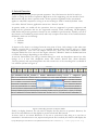
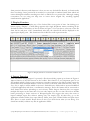
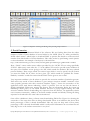
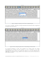
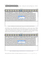
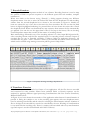
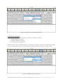
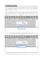
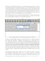
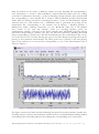
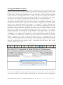
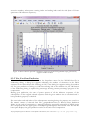
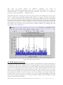
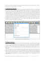
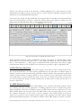
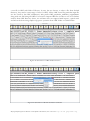
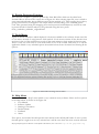
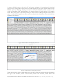
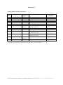
Laboratory of Natural Information Processing
DA-IICT Gandhinagar
Biospectrogram
User Manual
1 | Page Biospectrogram User Manual 1.0 Last updated on December 28, 2013. Visit us at h t t p : / / w w w . g u p t a l a b . o r g
BIOSPECTROGRAM
User Manual
© 2013 Manish K Gupta,
Laboratory of Natural Information Processing
DA-IICT, Gandhinagar, Gujarat 382007
http://www.guptalab.org/biospectrogram
The software described in this book is furnished under an open source license agreement and
may be used only in accordance with the terms of the agreement. Any selling or distribution of
the program or its parts, original or modified, is prohibited without a written permission from
Manish K Gupta.
Documentation version 1.0
This file was last modified on December 28, 2013.
Credits & Team
Principle Investigator: Manish K. Gupta, PhD.
Key Developers: Nilay Chheda* and Naman Turakhia*
Graduate Mentor: Vandana Ravindran
Supporting Developers: Ruchin Shah and Jigar Raisinghani
Software Logo: Hiren Kangad
* Key developers contributed equally to the project
Acknowledgments
We thank Deeksha Gupta for useful discussion in the early stage of the project. All the icons are taken
from the internet from the link “http://icons.mysitemyway.com/category/yellow-road-sign-icons/” These
icons are free to use for personal as well as commercial use “http://icons.mysitemyway.com/terms-of-use/”
MATLAB is registered trademark of Mathworks, USA. For FFT java script we thank Silvere Martin-
Michiellot and also to Craig A. Lindley whose open source code has been used with modifications.
2 | Page Biospectrogram User Manual 1.0 Last updated on December 28, 2013. Visit us at h t t p : / / w w w . g u p t a l a b . o r g
Table of contents
1. Introduction
2. Switch Function
3. Display Function
4. Import Function
5. Fetch Function
6. Manual Sequence Function
7. Encode Function
8. Transform Function
9. Window Analysis
9.1 Sliding Window Analysis
9.2 Stagnant Window Analysis
9.3 C, Yin, Yau Gene Prediction
10. NCBI Updates Function
11. Internet Connectivity Function
12. Preferences Function
13. Export Function
14. Clear History Function
15. ORF Finder Function
16. Protein Generator Function
17. Tools Menu
18. Help Menu
19. Application Directory Structure
20. Support Feedback and Distribution
References
Annexure 1: Some Popular Accession Numbers
Annexure 2: Transformation Quick Reference
04
06
07
07
08
10
11
11
12
13
16
17
18
19
20
20
21
21
23
23
23
25
25
26
27
28
3 | Page Biospectrogram User Manual 1.0 Last updated on December 28, 2013. Visit us at h t t p : / / w w w . g u p t a l a b . o r g
1. Introduction
Molecular biology has produced a vast amount of digital data in last decade. There is a need to
understand the genome of various species and plants. Mathematics, Computers Science and
Statistics are playing a major role in understand the data. One of the new branches has emerged
called genomic signal processing which employs digital signal processing (DSP) techniques to
study the spectral properties of the biological data and answer some biological questions. This is
done by converting the biological (DNA or protein) data into numerical data so that a DSP
technique can be applied for its analysis. Biospectrgram is open-source software to facilitate this
process. It applies 23 well-known encodings on the biological data and also performs 6
transformations. Using the user choice encodings, random encodings and other transformations
and filters available in MATLAB one can do tremendous spectral analysis. This document is
prepared to give users an overview of bio spectrogram software, utilities available in bio
spectrogram and motive behind the development of the software.
Entire software can be well understood by understanding its four major functionalities. (See
Figure 1)
1. Data Collector (Fetch/Import)
2. Encode
3. Transformation
4. Export
Data Collector
Encode
Transform
Export & Plot
Figure 1: Basic Building Blocks of Biospectrogram
Data Collector fetches the data from National Center for Biotechnology Information (NCBI)
server or a user can also import data from his own machine/network. Encoder module provides
20 different encodings on DNA data and 3 encodings on Protein data. User can apply following
transformation in Transformation module on the encoded data. The relationship between
encodings and transformations are given in Figure 2. The solid arrows represent transformations
available in Biospectrogram and broken arrow represents the transformation that can be applied
by MATLAB by exporting the encoded files from Biospectrogram. User can also export the
(both encoded and transformed) files to MATLAB files for plotting and further analysis. When
the application starts it shows the most recent fetched file in the upper pane.
Transformations that have been implemented in Biospectrogram are listed below:
1. Fast Fourier transform (T01)
2. Hilbert Transform (T02)
3. Z transform (T03)
4. Analytic Signal (T04)
5. Discrete Haar Wavelet (T05)
6. Chirp Z Transform (T06)
After installation of Biospectrogram, when it is executed for the first time, it will prompt user to
accept the license as shown in Figure 3. On accepting the license, user will be asked to enter total
RAM available on their system which can help software optimize the computation. If you are
using for the first time or if there are no files in your history then you will see the blank pane.
4 | Page Biospectrogram User Manual 1.0 Last updated on December 28, 2013. Visit us at h t t p : / / w w w . g u p t a l a b . o r g
Figure 2: Basic Relationships of Encodings and Transformations
Figure 3: License is shown at the first run of Biospectrogram
5 | Page Biospectrogram User Manual 1.0 Last updated on December 28, 2013. Visit us at h t t p : / / w w w . g u p t a l a b . o r g
2. Switch Function
Biospectrogram can also process protein sequences. Very first button in the left is used as a
switch to change the mode of operation. Right now we are supporting only two modes. One is
DNA mode and the other is protein mode. All the operation explained in the user manual
applies to only DNA sequences as long as we are working in “DNA” mode by default. Once
user clicks “Switch” button, application enters into “Protein” mode.
In protein mode, we enable all the operations that are supported to protein sequences and
disable all the operations that are not supported currently. Fetch, windowing, NCBI updates,
ORF finder and protein generator features are not available in protein mode. Actually, rest all of
the features are available in protein mode with only exception that three of the features behaves
differently which are as following:
1. Import
2. Encode
3. Display
In import a file, there is no change from the user point of view. Only change is that when user
imports a protein file, it should not go to standard fetched folder instead it will go to folder
“/History/Protein”. User can only import Protein file, fetch can only download or rather
recognize DNA files. You can see in the Figure 4 that the “Window” button is disabled and icon
of switch also changes depending on the mode it is in.
In encode functionality user will get similar dialog box with two dropdown menus but only
change in it is that first dropdown menu will contain Protein files (from directory
/history/protein) and second dropdown list will contain two of the encoding that is available in
our software (shown in Figure 4).
Figure 4: Encoding Function in Protein Mode
Finally, in display function, we only need to display the files that are in protein’s directory. So
that is the only difference in the display in protein mode and DNA mode.
In short, there is not much difference as far user is concerned. Only thing as a user has to
remember is that whenever a raw, unprocessed protein file is needed, the function will display list
6 | Page Biospectrogram User Manual 1.0 Last updated on December 28, 2013. Visit us at h t t p : / / w w w . g u p t a l a b . o r g
from protein’s directory and whenever it does not use any fetched files directly, its functionality
does not change. Once, protein file is encoded, it is converted to number format from which one
cannot distinguish whether encoding was done on DNA file or a protein file. Although, naming
conventions we are using can help user to know about original file, encoding applied,
transformation applied etc.
3. Display Function
This function is used to display any of the fetched files at any point of time. On clicking on a
button saying “Display”, a small dialog appears with single dropdown menu containing all the
fetched file names. Screenshot of that is shown in Figure 5. User just has to select any of the file
from the list and press “OK”. Immediately after that, the selected file will be displayed in the
upper input display pane. This function works in DNA as well as protein mode.
Figure 5: Display Function screenshot in DNA mode
4. Import Function
Once the button saying “Import” is pressed, a file chooser dialog opens up as shown in Figure 6.
Import function is the fifth button in the toolbar. This function is very important part of our
first module which is fetch as user can import customize sequences for analysis which cannot be
downloaded from standard database. Once user selects a file with valid extensions like .fasta, .fa,
.fna, .fsa, or .mpfa, it will be added to the user’s fetched history folder and on successful addition
of upload application will show a confirmation message. These all formats will be converted to
fasta format first before uploading to user’s history folder. Import function does not support
multiple file import at the same time. User can only import one file at a time. We wish to include
batch processing in future versions of Biospectrogram. We suggest that users who want to
import multiple input files without waiting they can simply copy all their files, go to the
application installer folder, then open History folder, then open Fetched folder and paste those
files. This is a work around. Please donot do this if you don’t know what you are doing. You
should not modify or delete any files in application folder.
7 | Page Biospectrogram User Manual 1.0 Last updated on December 28, 2013. Visit us at h t t p : / / w w w . g u p t a l a b . o r g
Figure 6: Snapshot showing the dialog after pressing import button
5. Fetch Function
“Fetch” forms very fundamental block of the software. We are fetching data from the online
database of DNA. Entire database is hosted online by the NCBI. There is a utility provided by
NCBI called “entrez” which helps to download DNA or protein files based on some accession
number from Nucleotide or Protein databases. This utility works by performing certain queries
on those databases. An example of such query is shown below:
http://eutils.ncbi.nlm.nih.gov/entrez/eutils/efetch.fcgi?db=protein&rettype=gb&retmode=text&id
Here, “Eutils” comes under entrez utilities provided by the “NCBI”. We are using specifically
“Efetch”. Main query starts after the “?” in the address. We need to provide some attributes in
the query. First attribute we are giving is the “db” which stands for database. We have selected
protein database. Then retype stands for retrieval type which is used to specify the file format
you want the DNA file in. Here we have given “gb” which stands for genbank file format.
Similarly “retmode” stands for retrieval mode which can be given as text or xml.
Very important attribute is the id where we provide the accession number of particular genome.
Each and every record of these databases is given unique accession number. Annexure-1 lists
some popular genomes with their accession numbers. Figure 7 shows the screenshot of the
application when sixth button indicating, “fetch” is pressed. You can see that the button is
slightly highlighted. When user presses that button, first an information dialog box opens up
describing e-fetch policy of the NCBI database and then a popup appears asking for valid
accession number. Before downloading any sequence from the internet, our application checks
user’s internet connectivity, validity of accession number entered and already existing file being
requested to download in the same order as mentioned.
Once all the validation is done, software starts downloading DNA files. Figure 8 is showing the
screenshot of the state when files are being downloaded. There is an indicator that shows how
much percentage of files is already downloaded. This way user can keep track of how many
percentage of file is already downloaded which is really useful information in case when files are
really big in size or the internet connection is very slow.
8 | Page Biospectrogram User Manual 1.0 Last updated on December 28, 2013. Visit us at h t t p : / / w w w . g u p t a l a b . o r g
Figure 7: Snapshot of pressing “fetch” button on Biospectrogram
If user press “CANCEL” while files are being downloaded, all downloads will be stopped and
incomplete files will be deleted.
Figure 8: Status of Biospectrogram when it is downloading a file from NCBI
On successful download of “fasta” and “genbank” file, software shows the prompt
acknowledging that operation has been successful. As soon as download is over, newly
downloaded fasta file is shown in the upper pane which acts as an input displaying pane.
Additionally, very first button saying “BACK” is also enabled once more than one files are in use
after software is started.
9 | Page Biospectrogram User Manual 1.0 Last updated on December 28, 2013. Visit us at h t t p : / / w w w . g u p t a l a b . o r g
6. Manual Sequence Function
On pressing the button saying “Manual Seq.”, a dialog box open up asking user to enter a
sequence manually as shown in Figure 9.
Figure 9: Importing a customized sequence (copy paste) via Manual sequence Button
User needs to copy a valid sequence (with valid characters A, C, G & T only in case of DNA
mode) and paste in the input box and press enter. After pressing OK, user will be asked to enter
a name for the sequence entered. On giving valid name, file will be created in the user’s history
folder and it will be displayed in the upper pane of the application as shown in Figure 10. This
feature can also be used to copy & paste a portion of genomic data from any file.
Figure 10: Snapshot showing customized sequence is saved in History folder
10 | Page Biospectrogram User Manual 1.0 Last updated on December 28, 2013. Visit us at h t t p : / / w w w . g u p t a l a b . o r g
7. Encode Function
Encoding is second most important module of our software. Encoding function is used to map
the symbols of DNA or protein sequence to the different spaces like real numbers, complex
numbers etc.
When user clicks on the button saying “Encode”, a dialog appears showing two different
dropdown menus. User has to select the fetched file from the first dropdown list and encoding
scheme from the second dropdown list as shown in the screenshot in Figure 11. Initially no
items are selected in any of two lists as shown in the first screenshot. We can see that the third
button is slightly highlighted indicating it is pressed. Here we have shown the screen shot of both
the dropdown menu. When user download any new sequence from internet the list automatically
get updated. User can also set the upper limit of files to be kept in the history. We are showing
second dropdown menu that contains all the names of encoding scheme.
Basic methodology followed in any of the encoding scheme is to select input DNA/protein file,
select encoding scheme and feed the required inputs for encoding scheme selected. Output of
encoded files are put in Encoded subfolder of History folder in application directory. All
encoded files are given “.fasta” extension. Name of the encoded file follow certain convention
which can be referred using naming convention pdf file given in Help folder.
Figure 11: Snapshot showing encodings dropdown list
8. Transform Function
Transformation is the third and a key feature of our application. All the files that are encoded
and converted in some number format from symbolic DNA or Protein sequence can be
analyzed by applying different signal processing transformations like Fast Fourier Transform,
Hilbert Transform etc.
In Figure 12, we have shown the screenshot of the application when button for transformation is
pressed. A dialog box similar to one in the encoding part appears with two dropdown menu.
One for selecting encoded file and the other for selecting the transformation scheme. Number of
files to be kept in the encoded list, can also be controlled by the user. Working of transformation
is very much like the encoding only. There is a unique code associated with every transformation
type and output is saved in Transformed sub folder of History.
11 | Page Biospectrogram User Manual 1.0 Last updated on December 28, 2013. Visit us at h t t p : / / w w w . g u p t a l a b . o r g
Figure 12: Snapshot for transformation button
9. Window Analysis
Window analysis feature provides three schemes for window analysis:
1.) Sliding Window Analysis
2.) Stagnant Window Analysis
3.) C, Yin,Yau Gene Prediction
When the user click on Window button, a dialog box appears as shown in the following Figure
13. This functionality tries to provide batch processing of windowed input of single strand.
Figure 13: Window analysis dialog box
12 | Page Biospectrogram User Manual 1.0 Last updated on December 28, 2013. Visit us at h t t p : / / w w w . g u p t a l a b . o r g
9.1 Sliding Window Analysis
Select a file for window analysis from the first drop down menu and select a windowing scheme
from the second drop down menu. When NC_001802.fasta (HIV-1 genome) is selected from
the first dropdown menu, and sliding window analysis is selected from the second drop down
menu and OK button is clicked, the a dialog box, shown in Figure 14, appears showing the
number of characters in the fasta file.
Clicking on OK button, a new dialog box, shown in Figure 15, appears asking if the user wants
to use a forward sliding window or a backward sliding window for analysis. Backward sliding
window will start from the end of the DNA sequence and move towards the start of the
sequence.
Figure 14: Number of characters in the fasta file selected for window analysis
Figure 15: Forward sliding window and backward sliding window option for sliding window analysis
13 | Page Biospectrogram User Manual 1.0 Last updated on December 28, 2013. Visit us at h t t p : / / w w w . g u p t a l a b . o r g
Selecting the forward sliding window option, a new dialog box appears asking the user to select
the encoding scheme and the transformation scheme to be used for window analysis. Selecting
the Indicator encoding for A from the first dropdown menu, and Fast Fourier Transform from
the second dropdown menu and clicking on OK, a new dialog box appears depicting the number
of characters in the file. Clicking on OK, another dialog box appears giving the user an option of
choosing a single window size or a range of window sizes. If a range of window sizes is chosen,
the user will be asked for the starting window size and ending window size for the range. If a
single window size is chosen, the user will be asked to enter a window size.
When starting window size is entered 300 and ending window size 302, the Biospectrogram
starts the sliding window analysis with forward sliding window in the window size range from
300 to 302 using Indicator encoding for A and Fast Fourier Transform.
Figure 16: Sliding window analysis showing percentage progress in computation
In this case, NC_001802 DNA sequence has 9181 characters. So, the selected encoding and
transformation will be applied to subsequences 1-300, thereafter 2-301,…, 8882-9181, 1-301, 2302, …, 8881-9181, 1-302, 2-303, …, 8880-9181. The percentage progress in the computation of
the encoding and transformation is shown in place of OK button in windowing dialog box. The
user can cancel the process at any time by clicking on the cancel button in the windowing dialog
box. In case of any other encoding or transformation scheme chosen, appropriate dialog boxes
will appear asking the user for parameters needed for the selected encoding and transformation.
At the end of the computation of encoding and transformations, a MATLAB script will be
generated for plotting all the transformation files for each window size in the range of window
sizes and a dialog box appears displaying information about names and location of the files
created in the process, and depicting successful generation of MATLAB script files with their
location.
For sliding window analysis option, subsequences of the selected DNA sequence are saved in
History/Window_Analysis/Fetched folder, with the naming convention, W<window
size>_<startIndex>_<input fasta file name>.fasta. For the above example, <window size> will
range from 300 to 302 and <startIndex> will range from 1 to 8882 for window size 300, 1 to
14 | Page Biospectrogram User Manual 1.0 Last updated on December 28, 2013. Visit us at h t t p : / / w w w . g u p t a l a b . o r g
8881 for window size 301 and 1 to 8880 for window size 302. Encoded file corresponding to
each subsequence is saved in History/Window_Analysis/Encoded folder with the naming
convention <subsequence file name>_<code for encoding scheme selected>.fasta. Transformed
file corresponding to each encoded file is saved in History/Window_Analysis/Transformed
folder with the naming convention <encoding file name>_<code for transformation scheme
selected>.fasta. For each window size, a MATLAB script is generated for plotting all the
transformed files corresponding to the window size in History / Window_Analysis /
Matlab_Files folder. Naming convention for the MATLAB script file is W<window
size>_<name of the fasta file selected>_<code for encoding scheme>_<code for
transformation scheme>_fasta.m. For the above example, three MATLAB script files will be
generated corresponding to window sizes 300, 301 and 302 respectively. Running MATLAB
script corresponding to window size 300 will automatically plot the transformation files one by
one at the interval of 0.2 second. Pressing the q key at any time during the plotting will stop the
plotting at that particular transformation file. When space bar is pressed, it will start plotting
again at the interval of 0.2 second. Plot corresponding to one of the transformation files is
shown in Figure 17.
Figure 17: Matlab plot obtained using the script generated by sliding window analysis
The figure contains axes labels and title indicating the input file accession number, window size,
encoding scheme selected, transformation scheme chosen, Forward/Backward sliding window
and starting index and ending index for the subsequence corresponding to the current plot.
15 | Page Biospectrogram User Manual 1.0 Last updated on December 28, 2013. Visit us at h t t p : / / w w w . g u p t a l a b . o r g
9.2 Stagnant Window Analysis
Stagnant window analysis can be used to extract a subsequence of the selected sequence and
generate power spectrum from all its indicator sequences. For example, suppose we have chosen
stagnant window analysis for NC_001802.fasta file. In the window analysis dialog box, when OK
is clicked after selecting NC_001802.fasta from first dropdown menu and Stagnant window
analysis from the second dropdown menu, a dialog box appears indicating the number of
characters in the selected DNA sequence. Clicking on OK, two new dialog boxes will appear,
one after the other, asking for starting index and ending index of the stagnant window.
Thereafter, a new dialog box appears asking if the user wants to generate a power spectrum of
the indicator sequences, which is the sum of the squares of magnitudes of Discrete Fourier
Transforms of all the indicator sequences. If the user chooses to generate power spectrum, OK
button in the windowing dialog box changes to “Analyzing…” thereby indicating that
computation is going on. As soon as computation is over, a dialog box displaying the successful
generation of power spectrum and MATLAB script to plot it along with paths of the
intermediate files generated will be displayed, as shown in Figure 18 and the subsequence will be
displayed on the upper pane of the Biospectrogram window. If the user chooses not to compute
the power spectrum, the subsequence will be displayed in the upper pane of the window.
Naming convention in the stagnant window analysis: Subsequence from starting index
<startIndex> to the ending index <endIndex> is saved in History/Fetched folder by the name
W_<startIndex>s_<endIndex>e_<input fasta file name>.fasta. If power spectrum is generated,
indicator sequences are saved in History/Encoded folder as <subsequence fasta file
name>_<indicator sequence code>.fasta and sum of power spectrum of all indicator sequences
is saved as: <subsequence fasta file name>_W01.fasta in History/Transformed folder. Matlab
script file for plotting power spectrum is saved as <subsequence fasta file name>_W01_fasta.m
in History/Matlab_Files folder.
Figure 18: Successful generation of power spectrum and MATLAB script file for plotting the spectrum
By running the MATLAB script generated by stagnant window analysis for NC_001802.fasta
file, the plot obtained is shown in Figure 19 along with the axes labels, and title containing the
16 | Page Biospectrogram User Manual 1.0 Last updated on December 28, 2013. Visit us at h t t p : / / w w w . g u p t a l a b . o r g
accession number, subsequence starting index and ending index and the title (Sum of Power
spectrum of all indicator sequences).
Figure 19: Sum of Power spectrum of indicator sequences plotted using Matlab script generated by
stagnant window analysis
9.3 C Yin, Yau Gene Prediction
When the user selects this feature from the dropdown menu for the X02323.fasta file in
windowing dialog, a dialog box appears indicating the number of characters in the DNA
sequence in the selected fasta file. Clicking on OK, a new dialog box appears asking for window
size for gene prediction. Clicking on OK after entering 300 as the window size, the OK button
of the windowing dialog is replaced by percentage showing current percentage progress of the
computation.
During gene prediction, the sum of power spectra of all the indicator sequences of the
subsequences of the original selected sequence with the given window size is calculated and 3base periodicity property is checked.
The start index and end index of the subsequences meeting having the property are saved in a
file named <name of selected fasta file>_geneprediction.fasta in History/Gene_Prediction
folder. At the end of computation, a message indicating successful generation of matlab script
file is displayed and the upper pane of BioSpectrogram displays the selected fasta file and the
lower pane displays the gene prediction results at the end of the computation.
17 | Page Biospectrogram User Manual 1.0 Last updated on December 28, 2013. Visit us at h t t p : / / w w w . g u p t a l a b . o r g
The
sum
of
power
spectra
of
indicator
sequences
are
saved
in
History/Gene_Prediction/Transformed folder with the name W<window size>_<name of
selected fasta file>_<startIndex>_W01.fasta, where startIndex varies from 1 to <number of
characters in selected sequence> - <window size>+1.
MATLAB script file for plotting the sum of the power spectra of all subsequences one by one is
saved in History/Gene_Prediction/Matlab_Files folder by naming convention W<window
size>_<name of selected fasta file>_W01_fasta.m. Running the Matlab script will automatically
plot sum of power spectra of indicator sequences of each subsequence one by one at the interval
of 0.2 second, one of which is shown in Figure 20. The user can stop the plotting at a particular
subsequence by pressing “q” and can resume the automatic plotting by pressing space bar. The
plot includes the axes labels along with accession number, window size, starting index and
ending index of the subsequence.
Figure 20: Sum of power spectra for subsequence 31-330 using C Yin, Yau Gene Prediction on
X02323.fasta with window size 300
10. NCBI Updates Function
Screenshots in Figure 21 shows the button to update the fetched history. Purpose behind this is
that database of the protein is highly dynamic. It keeps changing. So we have also provided utility
to update all the files in the user history at once. This simply re-downloads all the files that are in
the user history and replace them in place of older ones. This operation requires more time than
usual, so it is recommended that user perform this operation only when there is access of time
and internet speed. Figure 21 screenshot shows the same message so that user does not perform
this operation by mistake. For more security, we have put another yes/no input dialog after
pressing “OK” on this one. After user selects “yes”, we are simply downloading all files again
and on the successful updating we are showing confirmation dialog which will display message
saying all files updated successfully.
18 | Page Biospectrogram User Manual 1.0 Last updated on December 28, 2013. Visit us at h t t p : / / w w w . g u p t a l a b . o r g
Figure 21: Screenshot showing the NCBI update dialog
11. Internet Connectivity Function
The screenshot shown in Figure 22 shows the scenario when user presses the second last button
with @ symbol on it. This button checks the internet connectivity of the user. On pressing the
button application simply try to connect to the NCBI server itself because ultimately we also
need to check the whether the database server is up or not.
Figure 22: Screenshot for Internet connection is up dialog
You can see that the button is highlighted showing that is has been pressed. There is also tiny
message box displaying the status of user’s internet connection. Internet connection is required
19 | Page Biospectrogram User Manual 1.0 Last updated on December 28, 2013. Visit us at h t t p : / / w w w . g u p t a l a b . o r g
only of user needs to download some new files from NCBI server. This feature is also used by
default when user used “Fetch” functionality.
12. Preferences Function
After this, we have shown the screenshot of Preferences Dialog Box in Figure 23. Preference
box contains various preferences like checking amount of memory used for the fetched files,
encoded files, transformed files, maximum allowed files to be kept in the fetched, encoded and
transformed directory, check current maximum number of files allowed in fetched, encoded and
transformed directory and finally change the font size of the pane. Minimum value for font size
is 10 and the maximum it can take is 100. It also provides options to enter MATLAB plot delay
and custom RAM size allocation for Biospectrogram. If user enters invalid input, an error
message will show. In case user doesn’t remember the function of the buttons, there are tool tips
provided for the each and every button. If you look at the screen shot for the preferences box,
you will see very short description in the tool tip. After giving valid inputs, all the settings are
saved and message confirming that is displayed.
Figure 23: Screenshot showing preferences
13. Export Function
“Export” is final building block of our software which help output of encoded and transformed
files to save in the MATLAB file format so that user can further analyze by plotting graphs,
comparing graphs and using some other transformation techniques. This feature is developed in
the place of “Plot” functionality. Since we have all the output saved in proper format, we can
simply export it to the formats which can be plotted and analyzed in some other tools like
MATLAB.
Using this feature, user can create MATLAB script files to plot. As shown in the screenshot in
Figure 24, when a user clicks on Export to MATLAB button a dialog pops up showing one
dropdown menu. This pop up menu contains list of files which have been created after applying
some encoding and transformations. User can choose transformation file from there and click
“OK” button. This will create new script file with the name same as transformed file and
extension “.m”.
20 | Page Biospectrogram User Manual 1.0 Last updated on December 28, 2013. Visit us at h t t p : / / w w w . g u p t a l a b . o r g
All the “.m” files are saved in the directory “/History/Matlab_Files”. Same function can be
called from Tools Menu as well. User can click on “Tools->Export to Matlab” and get the same
dialog box for creating MATLAB script files.
As shown in the Figure 24, MATLAB files can be generated for encoded and transformed files
both. By selecting either of them, a simple file selector dialog will appear in which user can
simply select any file and click “OK” to create MATLAB script file.
Figure 24: Screenshot of MATLAB export button
After successful creation of file confirmation message will appear in seperate dialog. Since
MATLAB does not accept file names with “.” in the name, generated “.m” file will replace all the
dots (.) with underscore (_). Here export encoded file can be useful when user wants to apply
transformation which are not available in our software but possible to apply using MATLAB.
14 Clear History Function
This is a very simple function. As the name suggests, clear history button simply cleats all the
files in all the directories. It is like resetting application for the first time use. When clutter of
different fetched, encoded, transformed, exported to MATLAB files, files generated by different
window analysis reaches a situation which is out of control for user, this feature really comes
very handy. Since it can be harmful for some of the user as it deletes all the files, we have put
one extra confirmation dialog to decide whether user actually wants to delete all the files or it
was just a false click.
15. ORF Finder Function
ORF stands for open reading frame. ORF finding is very common and useful analysis used in
gene finding and other special applications for finding unknown areas of strand having some
special properties. There are six different types of ORF frames that are computed out of any
DNA strand. When user click the button for ORF Finder, they are asked if they want to enter
the sequence themselves or they want to choose sequence from fetched folder as shown in
Figure 25. User need to enter a sequence and a name of the sequence in the first option. Output
generated by Biospectrogram is very similar to NCBI’s online ORF Finder tool and it is saved as
21 | Page Biospectrogram User Manual 1.0 Last updated on December 28, 2013. Visit us at h t t p : / / w w w . g u p t a l a b . o r g
a text file in ORF sub folder of History. In case, the use chooses to select a file from fetched
directory, they need to enter range of sizes for ORF. All the ORF found for particular input file
are also saved in the ORF subdirectory with prefix ORF_startIndex_endIndex_originalName
along with text file listing all ORFs. User need to import ORF files in order to use it for further
analysis from ORF directory. Since, our software does not support batch import, a quick work
around can be done using simple copy-paste operation from ORF folder to fetched folder.
Figure 25: Screenshot of ORF Finder Function
Figure 26: Screenshot of Protein Generator Function
22 | Page Biospectrogram User Manual 1.0 Last updated on December 28, 2013. Visit us at h t t p : / / w w w . g u p t a l a b . o r g
16. Protein Generator Function
This function is helpful to generate protein files from DNA files which can be taken from
fetched folder as shown in the screen shot of Figure 26. After selecting input file, user is asked to
enter start and end index whose difference must be the multiple of 3. After entering those values,
group of three bases are mapped to the unique amino acid according to the standard genetic
code. Files generated using this mapping are stored in protein fetched directory and can be used
in protein mode for further analysis. Files generated using this have prefix
Gene_startIndex_endIndex_originalName.
17. Tools Menu
Figure 27 shows screenshot which displays Tools menu available in the software. Some users like
to use menus instead of using buttons with symbols. Tools menu contains all the function that
are there in the tool bar and behaves exactly in the same manner as their respective buttons part.
There is only one extra entry in tools menu which is not in the toolbar. That entry is to exit the
application which is very standard option. Screenshot below shows the menu bar showing all the
options.
Figure 27: Screenshot showing tool bar menu
18. Help Menu
Second menu is the “Help” menu which is very common in any software. There are four options
in the Help Menu as shown in the Figure 28.
1. User Manual
2. Software Update
3. Naming Conventions
4. Product Demo
5. Feedback
6. About
First option, user manual should open this user manual in the default pdf reader of user’s system.
Second option is right now not very relevant but it will be once there are more versions released.
23 | Page Biospectrogram User Manual 1.0 Last updated on December 28, 2013. Visit us at h t t p : / / w w w . g u p t a l a b . o r g
It opens a default browser in the user’s PC and opens a webpage of our application’s download
page. If user is using older version then he should upgrade to the newer version which can be
learned from that webpage. Naming conventions is another PDF file which contains all the
codes of Encodings and Transformations for quick reference. Fourth option is for product
demo. This entry opens a web URL pointing to video tutorial of Biospectrogram. Fifth option
opens a web based Google form where user can submit their feedbacks, views and criticisms
regarding our software.
Figure 28: Screenshot showing help menu bar
Figure 29: Screenshot showing about menu
Finally about option opens a small dialog box as shown in Figure 29, which contains information
like logo of the software, version of the software, name of the software, Credits button and
24 | Page Biospectrogram User Manual 1.0 Last updated on December 28, 2013. Visit us at h t t p : / / w w w . g u p t a l a b . o r g
homepage URL of the software. On pressing “Credits”, it opens a PDF document in user’s
default pdf reader.
19. Application Directory Structure
There is one root directory “Biospectrogram” which is the main application directory where
entire software is stored. There are four sub directory namely
1. History
2. Help
3. Icons
4. Source
History directory will have eight different subdirectories to organize different files for convenient
access. Four of them correspond to four main functions 1. Fetch 2. Encode 3. Transform 4.
Plot. There is one for Protein and two more directories for Window Analysis and Gene
Prediction and one for ORF. In Window analysis, there are again four sub directories for four
primitive functions of our application. In gene prediction, there are only two subdirectories one
for Transformed files and the other for export to MATLAB files.
Help directory contains all the help files in pdf format. Some of them are used in the application
and some of them are just for users’ general information. There are five files in total in Help
directory Coding conventions, User Manual, Credits files, Readme file and License file. Another
file named errors.log is created and updated dynamically as and when software runs into errors.
This file basically helps developers as well as user who themselves want to debug and tweak the
software for their own use.
Icons folder contains all the images used in the application. Source folder as the name suggest
contains all the source file essential for software. There are two build script one for Windows
and the other for Linux/MAC in the main application folder along with config file and some
other application related files. Do not touch them if you do not know what you are doing. It is
highly recommended that you do not temper with any of the files of any of the directories or sub
directories except History folder. If you break the software by playing with any of these files, just
backup your History folder, uninstall the application and then reinstall the application and
replace the History folder with your backed up one.
List of some popular accession numbers is given in Annexure 1 and Annexure 2 contains
formula used for different transformations in the application for the quick reference.
Windows version is compatible with all the Windows XP+ OS (32 & 64 bit). MAC version is
compatible with OS X+ OS (32 & 64 bit). You need to install java runtime version 1.7.0_45 or
above for windows and 1.7.0 for MAC. However, user who know basics about JAVA can
download zip version of source code and follow the instructions to run the software on any OS,
architecture with any JAVA version. Software is written in a way that it adapts to the native GUI
of the system.
20. Support, Feedback and Distribuation
Product demo video is available at the homepage of Biospectrogram. Users are requested to
contact Manish K. Gupta at the email: [email protected] for feedback and any other issues
with the software. A sample test data of genomes is available in the fetched folder of the
distributions of the software. We plan to have discussion forums etc. for users at the home page.
Enjoy the software!
25 | Page Biospectrogram User Manual 1.0 Last updated on December 28, 2013. Visit us at h t t p : / / w w w . g u p t a l a b . o r g
References
[1] M. Akhtar, J. Epps, and E. Ambikairajah. On DNA numerical representations for
period3 based exon prediction. In Genomic Signal Processing and Statistics, 2007. GENSIPS
2007. IEEE International Workshop, pp. 1 –4, June 2007.
[2] D. Anastassiou. Genomic signal processing. Signal Processing Magazine, IEEE, 18(4):8– 20,
Jul 2001.
[3] A. K. Brodzik and O. Peters. Symbol-balanced quaternionic periodicity transform for
latent pattern detection in DNA sequences. In Proceedings. (ICASSP ’05). IEEE
International Conference on Acoustics, Speech, and Signal Processing, 2005., pp.
373– 376. Philadelphia, Pennsylvania, USA, IEEE, 2005.
[4] N. Chakravarthy, A. Spanias, L. D. lasemidis, and K. Tsakalis. Autoregressive modeling
and feature analysis of DNA sequences,. EURASIP JASP,, 1:13–28, 2004.
[5] P.D. Cristea. Phase analysis of DNA genomic signals. Proceedings of the
Symposium on Circuits and Systems, 2003. ISCAS ’03., 5:V–25–V–28, 2003.
International
[6] Paul Dan Cristea. Large scale features in DNA genomic signals. Signal Process., 83(4):871–
888, April 2003.
[7] B. Liao. A 2d graphical representation of DNA sequence,. Chem Phys Lett,, 401:196– 199,
January 2005.
[8] J. Ning, C.N. Moore, and J.C. Nelson. Preliminary wavelet analysis of genomic
sequences. In Bioinformatics Conference, 2003. CSB 2003. Proceedings of the 2003 IEEE, pp.
509–510, Aug. 2003.
[9] N. Rao and S.J. Shepherd. Detection of 3-periodicity for small genomic sequences based
on ar technique. In Communications, Circuits and Systems, 2004. ICCCAS 2004. 2004
International Conference on, volume 2, pp. 1032 – 1036 Vol.2, June 2004.
[10] G. L. Rosen. Signal processing for biologically inspired gradient source localization and
DNA sequence analysis,. PhD thesis, Georgia Institute of Technology,, Aug. 2006.
[11] B. D. Silverman and R. Linsker. A measure of DNA periodicity. Journal of Theoretical
Biology, 118:295–300, 1986.
[12] P. P. Vaidyanathan. Genomics and proteomics: A signal processors tour. IEEE Circuits
Syst. Mag, 4:6–29, 2005.
[13] Richard F. Voss. Evolution of long-range fractal correlations and 1/f noise in DNA
base sequences. Physical Review Letters, 68(25):3805+, June 1992.
[14] S. T. Yau, J. Wang, A. Niknejad, C. Lu, N. Jin, and Yee-Kin Ho. DNA sequence
representation without degeneracy. Nucleic Acids Research, 31(12):3078–3080, June 2003.
[15] R. Zhang and C. T. Zhang. Z curves, an intuitive tool for visualizing and analyzing the
DNA sequences. J. Biomol. Struct. Dyn., 11(4):767–782, 1994.
[16] Zhu-Jin Zhang. DV-curve: a novel intuitive tool for visualizing and analyzing DNA
sequences. Bioinformatics, 25(9):1112–1117, March 2009.
26 | Page Biospectrogram User Manual 1.0 Last updated on December 28, 2013. Visit us at h t t p : / / w w w . g u p t a l a b . o r g
Annexure-1
Some popular accession numbers*
Sr.
No.
1
2
3
4
5
6
7
Organism
Phage phiX174
Human mtDNA
Lambda Phage
HIV
H. influenzae
M. genitalium
S. cerevisiae
8
9
10
E. coli K12
C. trachomatis
D. melanogaster
Size
(Approx.)
5368 bp
16571 bp
48502 bp
9193 bp
1830 Kb
580 Kb
12.5 Mb
total size
4.6 Mb
1042 Kb
180 Mb
11
A. thaliana
125 Mb
12
H. Sapiens
13
SARS
3000 Mb
total size
29751 bp
Description
1st Viral genome
1st Organelle genome
Important virus model
AIDS retrovirus
1st bacterial genome
Smallest bacterial genome
1st eukaryotic genome
(Chromosome XV)
Bacterial model organism
Internal parasite of eukaryotes
Fruit fly, model insect
((Chromosome 2L)
Thale cress, model plant
(Chromosome III)
Human (Chromosome XI)
Coronavirus
Accession
Number
NC_001422.1
NC_012920.1
NC_001416.1
NC_001802.1
NC_016809.1
NC_000908.2
NC_001147.6
NC_000913.2
AE001273.1
NT_033779.4
NC_003074.8
NT_009237.18
NC_004718.3
* User can find more accession numbers from the entrez browser at NCBI.
27 | Page Biospectrogram User Manual 1.0 Last updated on December 28, 2013. Visit us at h t t p : / / w w w . g u p t a l a b . o r g
Annexure-2
For a sequence of N complex numbers
Transform
Fast Fourier Transform
Discrete Haar Wavelet
Transform
Hilbert transform in
frequency domain
Analytic Signal
,
Formula
,
Remarks
N is a power of 2. If
length of sequence is not
a power of 2, it is zero
padded to make its
length equal to the
nearest power of 2
2,approximation coefficients
where
is a low pass
2 , detailed coefficients
filter where as
pass filter.
is a high
where u(n)=
is the
input sequence
where
is Hilbert
transform of input
sequence
domain
in time
Z transform
Chirp Z transform
If contour is a circle of
radius r and are N
equally spaced points,
then
.
Biospectrogram provides
following variables:
, where
.
Providing u=1, v=N as
input will give N equally
spaced points on the
circle of radius a.
28 | Page Biospectrogram User Manual 1.0 Last updated on December 28, 2013. Visit us at h t t p : / / w w w . g u p t a l a b . o r g