Download Sample Curricula. - Industrial Fiber Optics

*
Copyright © 2011
Previous Printings 2001, 1992, 1990, 1989
By Industrial Fiber Optics, Inc.
Revision B
Printed in the United States of America
*
*
*
All rights reserved. No part of this publication may be reproduced,
stored in a retrieval system, or transmitted in any form or by any
means (electronic, mechanical, photocopying, recording, or
otherwise) without prior written permission from Industrial Fiber
Optics, Inc.
*
*
INDUSTRIAL FIBER OPTICS
1725 West 1st Street
Tempe, AZ 85281-7622
USA
*
*
*
Table of Contents
History & Introduction to Fiber Optics..............................................................
1
Fiber Optic Communications ...........................................................................
3
Review of Light & Geometric Optics................................................................
6
The Fundamentals of Optical Fibers ...............................................................
8
Light Sources & their Characteristics ..............................................................
11
Transmitter Components.................................................................................
14
Detectors for Fiber Optic Receivers ................................................................
16
Elements of Fiber Optic Receivers..................................................................
18
Passive Optical Interconnections. ...................................................................
20
Fiber Optic System Design & Analysis ............................................................
23
Fiber Optic Test Equipment & Tools................................................................
25
Industrial Applications of Fiber Optics .............................................................
27
Lab Session I ..................................................................................................
32
Lab Session II .................................................................................................
34
References......................................................................................................
36
Glossary ..........................................................................................................
37
This publication serves as an introduction to fiber optics for instructors and their
students. It addresses the subject with basic mathematical formulas and includes
principles of fiber optics, its components (such as the fiber itself, receivers and
transmitters), system design, completed systems, test equipment and industrial
applications. The main section of the handbook is followed by two lab sessions, list of
references (books, magazines and professional organizations), and a glossary of fiber
optic terms used in the handbook and in the field of fiber optics. No prior knowledge of
this subject is needed to understand and use this handbook. It will serve as a useful
reference for the professional and student as fiber optics becomes a part of their
everyday lives.
i
Warranty Information
This kit was carefully inspected before leaving the factory. Industrial Fiber Optics products are warranted
against missing parts and defects in materials for 90 days. Since soldering and incorrect assembly can
damage electrical components, no warranty can be made after assembly has begun. If any parts become
damaged, replacements may be obtained from most radio/electronics supply shops. Refer to the parts list
on page 32 of this manual for identification.
Industrial Fiber Optics recognizes that responsible service to our customers is the basis of our continued
operation. We welcome and solicit your feedback about our products and how they might be modified to
best suit your needs.
ii
HISTORY & INTRODUCTION TO FIBER OPTICS
History of Fiber Optics
Fiber optics is essentially a method of carrying information
from one point to another. An optical fiber is a thin strand of
glass or plastic over which information passes. It serves the
same basic function as copper wire, but the fiber carries light
instead of electricity. In doing so, it offers many distinct
advantages which make fiber optics the best transmission
medium in applications ranging from telecommunications to
computers to automated factories.
Using light for communications is not new. In the United
States, lanterns hung in a church signaled Paul Revere to begin
his famous ride. Ships have used light to communicate
through code, and lighthouses have warned of danger and
greeted sailors home for centuries.
Claude Chappe built an optical telegraph in France during
the 1790s. Signalmen in a series of towers stretching from
Paris to Lille, a distance of 230 km, relayed signals to one
another through movable mechanical arms. Messages could
travel from end to end in about 15 minutes. In the early years
of the United States, an optical telegraph linked Boston and a
nearby island. These systems were later replaced by electric
telegraphs.
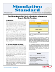
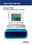
A basic fiber optic system is a link connecting two
electronic circuits. Figure 1 shows the main parts of such a
link:
Transmitter, which converts an electrical signal into a
light signal. A “source” (either a light emitting diode or laser
diode) does the actual conversion. A drive circuit changes the
electrical signal fed to the transmitter into a form required by
the source.
The English natural philosopher John Tyndall, in 1870,
demonstrated the principle of guiding light through internal
reflections. In an exhibition before the Royal Society, he
presented light bending around a corner as it traveled in a jet of
pouring water. Water flowed through a horizontal spout near
the bottom of a container, along a parabolic path through the
air, and down into another container. When Tyndall aimed a
beam of light out through the spout along with the water, his
audience saw the light following a path inside the curved path
of the water.
Fiber optic cable, the medium for carrying the light. The
cable includes the fiber and its protective covering.
Receiver, which accepts the light and converts it back to
an electrical signal. The two basic parts of a receiver are the
detector, which converts the light signal to an electrical signal,
and the output circuit, which amplifies and, if necessary,
reshapes the electrical signal before passing it on.
Connectors, which connect the fibers to the source,
detector and other fibers.
As with most electronic systems, the transmitter and
receiver circuits can be very simple or very complex.
TRANSMITTER
Signal
In
Driver
Light
Source
Source-to-fiber
connection
Fiber
Optic Cable
RECEIVER
Amplifier
Detector
Fiber-to-detector
connection
1363.eps
Signal
Out
Figure 1. Components found in a basic fiber optic data link.
-1-
In 1880, an engineer named William Wheeler patented a
scheme for piping light throughout a building. Not believing the
incandescent bulb practical, Wheeler planned on using light
from a bright electrical arc to illuminate distant rooms. He
devised a series of pipes with reflective lining to be used inside
the building.
Studies of how to control and use light continued through
the twentieth century. Interest in glass waveguides increased in
the 1950s, when research turned to glass rods for transmission
of images. These are known as "fiberscopes" today, and are
widely used in medicine. The term "fiber optics" was coined in
1956 with the invention of glass-coated rods.
In 1966, scientists at ITT proposed glass fiber as a
transmission medium. Then, fiber had losses greater than
1000 dB/km. They determined if losses could be reduced to
20 dB/km, a level considered obtainable and quite suited for
communication, fiber optic data communication would be
practical. Today, losses in the best fibers are around 0.2
dB/km.
During the 1960s, many companies laid the groundwork
to make them leaders in fiber optic technology. Corning Glass
Works produced the first 20 dB/km fiber in 1970, and by
1972 losses were down to 4 dB/km. AMP produced the first
low-cost fiber optic connector in 1974. In 1979 the fiber-optic
pigtail was introduced by a joint effort of Motorola and AMP.
The Navy installed a fiber optic link aboard the USS Little
Rock in 1973. The Air Force replaced the wiring harness of an
A-7 aircraft in 1976. The original wiring harness had 302 cables
and weighed 40 kg. The optical replacement had 12 fibers and
a weight of 17 kg. The military was also responsible for one of
the first operational fiber optic data links in 1977 — a 2 km,
20 Mbps (million bits per second) system for a satellite earth
station.
The Bell System installed the first trial fiber optic
telephone link at the Atlanta Works in 1976. The first field
commercial trial occurred in 1977 near Chicago. It was a 44.7
Mbps, 2.5 km system with an outage rate of 0.0001% at the
end of one year. (The Bell requirement was 0.02%.) In 1980,
Bell announced a 1000 km project from Cambridge, MA, to
Washington, DC.
Today these projects are history and fiber optics is a
proven technology. Nevertheless, many new and exciting
applications are currently being developed and the future is
bright for many more.
Advantages
The answer lies in the following advantages of fiber optics.
• Wide bandwidth
• Low loss
• Electromagnetic immunity
• Security
• Light weight
• Small size
• Safety and electrical isolation
The importance of each advantage is applicationdependent. In some cases, the wide bandwidth and low loss
of fiber optics is the overriding factor. In others, security or
safety are the determining factors. More details about the
benefits of fiber optics will be covered in the next chapter.
Applications
A wide variety of fiber optic systems have been developed
through many years of work. Examples of current fiber optic
systems include:
• Long-haul telecommunications systems on land or at sea
to carry many simultaneous calls over long distances
• Interoffice trunks carrying many simultaneous telephone
conversations between local and regional telephone
switching facilities
• Telephone lines with much higher speed than common
single telephone lines
• Connections between microwave receivers and control
facilities
• Links among computers and high-resolution video
terminals used for such purposes as computer-aided
design
• Cable television
• High-speed local-area networks
• Portable battlefield communication equipment
• Fiber optic gyroscopes for navigation
• Temperature, pressure, magnetic and acoustic sensors
• Illumination and imaging systems
Much of the early use of fiber optics involved data
communications. Today, a significant amount of research is
being conducted on developing fiber optic sensors. For
example, concepts are being tested using optical fibers in
aircraft wings and bridges to monitor stress. Optical fiber
sensors have the unique advantage of being able to be used in
very hostile environments such as high temperatures or in
explosive gases.
In its simplest terms, fiber optics is a communication means
to link two electronic circuits. The fiber optic link may be
between a computer and its peripherals, between two
telephone switching offices, or between a machine and its
controller in an automated manufacturing facility. Obvious
questions concerning fiber optics are: Why go to all the trouble
of converting the signal to light and back? Why not just use
wire?
-2-
FIBER OPTIC COMMUNICATIONS
This chapter introduces the important aspects of signals
and their transmission. An understanding of the underlying
principles of modern electronic communication is fundamental
to understanding and appreciating fiber optics. The ideas
presented here are fundamental not only to fiber optics, but
also to all electronic communications.
Communications
Communication is the process of establishing a link
between two points and passing information between them.
Information is transmitted in the form of a signal. In
electronics, a signal can be anything from the pulses running
through a digital computer to the modulated radio waves of an
FM radio broadcast. Such passing of information involves
three activities: encoding, transmission and decoding.
1275.eps
Encoding is the process of placing information on a
carrier. The vibration of your vocal cords places the code of
your voice on air. Air is the carrier, changed to carry
information by your vocal cords. Until it is changed in some
way, a carrier contains no information. A steady oscillating
wave electronic frequency can be transmitted from one point
to another, but it contains no information unless data is
encoded on it in some way. Conveying information, then, is
the act of modifying the carrier. This modification is called
modulation.
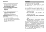
The creation of a signal by impressing information on a
carrier is shown in Figure 2. The high-frequency carrier, which
in itself contains no information, has impressed on it a lowerfrequency signal. The shape of the carrier is now modulated by
the information. Although the simple example in the figure
conveys very little information, the concept can be extended to
convey a great deal. A Morse Code system can be based on
the example shown. On the carrier, a low-frequency
modulation can be impressed, with one or two periods in
length corresponding to dots and dashes, respectively.
Once information has been encoded by modulating the
carrier, it is transmitted. Transmission can occur over air,
copper cables, through an optical fiber, or any other medium.
Figure 2. Basic modulation of signals.
At end of transmission, the receiver separates the
information from the carrier in the decoding or demodulation
process. A person's ear separates the vibrations of the air and
turns then into nerve signals. Radio receivers strip away the
high frequency carrier, while keeping the audio frequencies for
further processing. In fiber optics, light is the carrier on which
information is impressed.
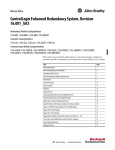
There are three basic ways to modulate the carrier. See
Figure 3 for examples.
Amplitude Modulation (AM) - A signal that varies
continually (e.g., sound waves).
Frequency Modulation (FM) - Frequency modulation
changes the frequency of the carrier to correspond to the
differences in signal.
Digital Modulation - Signals that have been encoded in
discrete levels, typically binary ones and zeros.
Amplitude Modulation (AM)
The world around us is analog. "Analog" implies
continuous variation, like the moment of hands on a clock.
Sound is analog. Ocean waves are analog. Analog is the
variation of the amplitude in the medium. Before the invention
of digital logic, everything was analog. In fact, the very first
computers were analog.
-3-
Frequency Modulation (FM)
This type of modulation is used least in fiber optics due to
difficulty of implementation. The transmitter must emit a
single frequency and be stable. To demodulate an FM
transmission a local optical oscillator must be used, and the
oscillator must have a wavelength identical to that of the
transmitter. FM radio does not suffer from these adverse
characteristics, since radio frequencies are five decades lower
and frequency control of electrical signals has been mastered.
Frequency modulation, however does offer the largest
information bandwidth capabilities, and researchers are actively
developing FM fiber optic links. Theoretical studies and
demonstration systems have been constructed. Today, there
are no commercial FM optical links in use, but students of
today will see them in years to come.
Digital Modulation
The word "digital" implies numbers — distinct units, like
the display of a digital watch. In a digital system, all
information exists in numerical form.
The bit, the fundamental unit of digital information, has
two states; a one or zero. In electronics, the presence or
absence of a voltage is the most common digital
representation. Unfortunately, the single bit 1 or 0 can
represent only a single state, such as on or off. A single bit
has limited usefulness. Extending the number of bits increases
the amount of information. For example, a three-way
household lamp can have four states:
Off = 00
On = 01
Brighter = 10
Brightest = 11
The more bits in a unit, the more potential information
can be expressed. A digital computer typically works with units
of eight bits (or multiples of eight). Eight bits permits 256
different meanings in a given pattern of 1s and 0s. This can
communicate all the characters of the number system and
upper and lower case letters of the alphabet.
Information in digital systems is transferred by pulse trains
as shown in Figure 3 (c).
(a)
(b)
(c)
1276.eps
Figure 3. Types of modulation (a) AM, (b) FM, (c) digital modulation.
-4-
Advantages
The introductory section of this handbook listed and
introduced the advantages of fiber optics. Following is a more
detailed description of optical fiber's advantages.
Bandwidth
The information-carrying capacity of a carrier wave
increases with the carrier frequency. The carrier wave for a fiber
optic signal is light, and is several orders of magnitude higher in
frequency than the highest radio wave. Fibers have higher
bandwidths, which allows for very high-speed transfer of data.
With multiplexing, several channels can be sent over a single
fiber. In computers, for instance, the capability of multiplexing
paralleled bus lines into serial form for transmission over a
fiber can reduce hardware and cabling costs. In telephony, a
fiber optic system can carry 672 voice channels one way in a
single line. Planned optical multiplexing techniques, such as
wavelength division multiplexing, will increase this capacity to
thousands of voice channels.
Weight
A glass fiber optic cable with the same information-carrying
capacity as copper cable weighs less than copper cable because
the copper requires more lines than the fiber. For example, a
typical single-conductor fiber cable weighs 1.2 kg/km. A
comparable coaxial cable weighs nine times as much - about 10
kg/km In applications such as ships and aircraft, weight
savings allow for more cargo, higher altitude, greater range, or
more speed.
Small Size
A fiber optic cable is smaller than its copper equivalent,
and a single fiber can often replace several copper conductors.
A fiber optic cable containing 144 fibers in a 12 mm diameter
has the capacity to carry 24,192 conversations on a single
fiber, or nearly two million calls on all the fibers. A comparable
coaxial cable would be about nine times larger.
Optical fibers have potential frequency ranges up to about
1 Terahertz, although this range is far from being exploited
today. The practical bandwidth of an optical fiber greatly
exceeds that of copper cable. Furthermore, the bandwidth of
fiber optics has only begun to be utilized, whereas the potential
of copper cable is nearing its limits.
Low Loss
Loss determines the distance that information can be sent.
As signals travel along a transmission path (copper or fiber),
they lose strength. This loss is called attenuation. In a copper
cable, attenuation increases with frequency: the higher the
frequency of the carrier signal, the greater the loss. In an optical
fiber, the attenuation is flat; loss is the same up to very high
modulation frequencies.
Electromagnetic Immunity (EMI)
Because fiber is a dielectric, it is not affected by ordinary
electromagnetic fields. This offers several advantages over
copper cables. Any copper conductor acts as an antenna, either
transmitting or receiving. This can cause the quality of data
being transmitted or received to be degraded, or in the
extreme, lost. EMI control for copper wires commonly
involves adding shielded or coaxial cables. The increased
shielding raises costs, making fiber system more competitive,
and still does not totally alleviate the EMI problem.
Security
It is virtually impossible to "tap" a fiber optic cable
surreptitiously, because attempts to reach the light-carrying
central portions of the fiber generally affect
transmission enough to be detectable. Since fiber does not
radiate energy, other eavesdropping techniques fail. Such
security reduces data encryption costs.
-5-
REVIEW OF LIGHT & GEOMETRIC OPTICS
Light travel through an optical fiber depends on the basic
principles of optics and light’s interaction with matter. The first
step in understanding fiber optics is to review light and optics.
From a physical standpoint, light can be represented either as
electromagnetic waves or as photons. This is the famous
“wave-particle duality theory” of modern physics.
The relationship between frequency and wavelength of
light is defined by Equation 1,
! =
Light also exhibits some particle-like properties. A light
particle is called a photon, a discrete unit of energy. The
amount of energy contained by a photon depends on its
wavelength. Light with short wavelengths has higher energy
photons than does light at longer wavelengths. The energy E,
in joules, contained in a photon is
Many of light's properties can be explained by thinking of
light as a wave within the electromagnetic spectrum. This
spectrum is shown in Figure 4. Light is higher in frequency and
shorter in wavelength than the more common radio waves.
Visible light is from 380 nanometers (nm), far deep violet, to
750 nm, far deep red. Infrared radiation has longer waves than
visible light. Most fiber optic systems use infrared light
between 750 and 1500 nm. Plastic optical fiber operates best
in the 660 nm red wavelength region.
!
Gamma rays
1020
! (nm)
380
h • c
f
Equation 2
h is Planck's constant, which is 6.63
Treating light as both a wave and as a particle aids
understanding of fiber optics. It is necessary to switch between
the two descriptions to understand the different effects. For
example, many properties of optical fiber vary with
wavelength, so the wave description is used. In the case of
optical detectors, responsivity to light is best explained with
the particle theory.
1021
X-rays
=
where f is frequency and
X 10-34 joule-seconds.
Frequency (Hz)
1019
Equation 1
where c is the speed of light and f is frequency.
Light
1022
c
f
Ultraviolet
1018
1017
1016
1015
Ultraviolet
Visible
600
Orange (620)
14
10
1013
Violet (455)
Blue (490)
Green (550)
Yellow (580)
Infrared
Red (680)
1012
1011
1010
800
Refractive Index
The most important optical measurement for any
transparent material is its refractive index ( ! ). Refractive index
is the ratio of the speed of light in a vacuum to the speed of
light in the transparent material.
! =
Infrared
Microwave
c
c
vacuum
Equation
3
material
109
108
The speed of light through any material is always slower
than in a vacuum, so a material's refractive index is always
greater than one. In practice, the refractive index is measured
by comparing the speed of light in the material to that in air,
rather than in a vacuum. This simplifies the measurements and
does not make any practical difference, since the refractive
index of air is very close to that of a vacuum. See Table 1.
107
106
Radio waves
105
104
103
102
Power and telephone
1001.eps
101
Figure 4. The electromagnetic spectrum.
-6-
Table 1. Refractive Indices of Some Common
Materials.
Material
Refractive Index
Vacuum
1.0
Air
1.00029
Water
1.33
Fused Quartz
1.46
Glass
1.45 - 1.6
Diamond
2.0
Silicon
3.4
Gallium Arsenide
3.6
reflected when the reflected angle equals or is greater than the
angle of incidence. This phenomenon is called total internal
reflection. Total internal reflection is what keeps light confined
to an optical fiber. The critical angle above which total internal
refection occurs can be derived from Snell's Law.
!
Equation 4
where ! 1 and ! 2 are the refractive indices of the initial and
secondary mediums, respectively. The angles ! 1 and ! 2 are
the angles from normal of the light rays in initial and secondary
materials respectively.
Normal line
Equation 5
The numerical aperture (NA) of a fiber is related to the
critical angle and is the more common way of defining this
aspect of a fiber. Critical angles of fibers are not normally
specified. Calculation of the numerical aperture of an optical
fiber, using the index of refraction of the core and the cladding,
can be done with Equation 6.
Light travels in straight lines through most optical
materials, but something different happens at the point where
different materials meet. Light bends as it passes through a
surface in which the refractive index changes — for example,
passing from air into glass, as shown in Figure 5. The amount
of bending depends on the refractive indices of the two
materials and the angle of the incident ray striking the
transition surface. The angles of incidence and transmission are
measured from a line perpendicular to the surface. The
mathematical relationship between the incident and transmitted
rays is known as Snell's Law.
Incident ray
#" 2&
= arc sin %
(
$" 1'
Numerical Aperture
Snell's Law
!1 " sin # 1 = ! 2 " sin # 2
critical
Reflected ray
!" =
(#
2
0.5
Equation 6
Another term that is sometimes useful is acceptance angle,
which can be obtained from the numerical aperture.
!
acceptance
= arc sin "#
Equation 7
Acceptance angle is the half cone angle of the light that can
be sent into an optical fiber and be reflected internally. The
numerical aperture and acceptance angles of fibers are used for
analyzing the collection efficiency of light sources and detectors.
Fresnel Reflections
Even when light passes from one index to another, a
small portion is always reflected back into the first material.
These reflections are known as Fresnel reflections. The greater
the difference in the indices of the two materials, the greater
the reflection. The magnitude of the Fresnel reflection at the
boundary between any two surfaces is approximately:
"1
R =
Medium 1: air (n 1)
(! " ! )
(! + ! )
1
1
Medium 2: water (n 2)
)
$ # cladding
2
core
2
Equation 8
2
2
2
Light passing from air into an optical fiber and back to air
has double this loss.
"2
Refracted
ray
1000
Figure 5. Optical rays at optical interface.
Critical Angle
Snell's law indicates that refraction cannot take place when the
angle of incidence becomes too large. (Light traveling from a
high index to a low index.) If the angle of incidence exceeds
the critical value, where the sine of the angle equals one, light
cannot exit the glass. (Recall from trigonometry that the
maximum value of the sine of 90 degrees is 1.) All power is
-7-
THE FUNDAMENTALS OF OPTICAL FIBERS
Construction
Fiber Types
The simplest fiber optic cable consists of two concentric
layers. The inner portion, the core, carries the light. The
outer covering is the cladding. The cladding must have a
lower refractive index than the core; therefore, the core and
cladding are never exactly the same material.
In defining fiber types, we will not use physical materials
for classification. Fiber types are classified according to the
type of mode structure and light passage paths in the fiber.
The three fiber types are step-index, graded-index and singlemode. (See “mode” in the Glossary.)
A cross section of an optical fiber is shown in Figure 6.
A light ray, within the acceptance angle, travels down the
fiber. Light striking the core-cladding interface at less than the
critical angle passes into the cladding. The cladding is usually
optically glossy or opaque to dissipate light launched into the
cladding. If these rays were allowed to travel down the
cladding, the fiber bandwidth would be severely degraded.
Step-index Fiber
Step-index fiber was the first fiber developed and the
simplest of the three types. It has many modes depending on
the size and numerical aperture. A step-index fiber is depicted
in Figure 6. The diameter of this type of fiber ranges from 50
µm to 13 cm. It suffers from having the lowest bandwidth
and greatest loss. The lowest dispersion is about 15
nanoseconds/km. (Lower dispersion is better; this will be
covered later.)
1348.eps
Cladding
Core
Graded-index Fiber
In a step-index optical fiber, the higher-order modes
travel farther distance than lower modes as they bounce
down the optical fiber. To overcome this lengthening effect,
a graded refractive index core was developed. This
construction is similar to having many concentric cylinders or
tubes of optical material. Figure 7 (a) shows the refractive
index profile and light rays traveling in the fiber. The outer
layers have a lower refractive index to "speed up" these light
rays, compensating for the greater distance traveled. Modal
dispersion in this type of fiber is 1 nanosecond/km.
Figure 6. Cross-section of an optical fiber (step-index).
Light travel in an optical fiber depends upon several
factors:
• Size of fiber
• Numerical aperture
• Material
• Light source
Single-mode Fiber
Modes
This fiber construction only allows a single mode to pass
efficiently. The core is very small, only 5 to 10 µm in
diameter. A single-mode fiber is shown in Figure 7 (b). Singlemode fibers have a potential bandwidth of up to 100 GHzkm.
The "mode" is an abstract concept originating from
mathematicians that lets physicists describe an occurrence in
electromagnetic theory. Mode theory can be applied to
Maxwell's equations on electromagnetic energy. Maxwell's
equations simply state: The boundary conditions of an
electromagnetic waveguide determine the characteristics of
light’s passage. As it turns out for many of the world’s
conditions, including fiber optic cables, many simultaneous
solutions to Maxwell's equations exist. Each solution is
different, and each solution is called a mode.
For a fiber to behave as a single mode, the diameter of
the core must be very close to the same size as the
wavelength of the optical carrier. The cladding of an optical
fiber must be greater than 10 times thicker than the core to
satisfy the boundary conditions of Maxwell's equations. A
single-mode fiber at 1300 nm may not be single-mode at 820
nm. Most commonly available single-mode fibers are for
1300 and 1500 nm systems.
A mode traveling in a fiber cable has a finite path and a
characteristic energy defined by Maxwell's equations. Optical
fibers can sustain as few as one mode to greater than
100,000. The low-order modes travel near the center of the
core and the higher-order modes are those traveling closest to
the critical angle.
-8-
1277.eps
Cladding
The dispersion of optical energy falls into two categories:
modal dispersion and spectral dispersion.
Core
(a)
Fiber
Cladding
1278.eps
Core
1279.eps
Figure 8. Dispersion in an optical fiber.
(b)
Modal Dispersion
Figure 7. (a) Graded index and (b) single mode fiber.
Light travels a different path for each mode in a fiber.
Each path varies the optical length of the fiber for each
mode. In a long cable, the stretching and the summing of all
a fiber's modes have a lengthening effect on the optical pulse.
Attenuation
Light transmission by optical fiber is not 100 percent
efficient. Light lost in transmission is called attenuation.
Several mechanisms are involved — absorption by materials
within the fiber, scattering of light out of the fiber core, and
leakage of light out of the core caused by environmental
factors. Attenuation depends on trans-mitter wavelength
(covered in more detail later).
Spectral Dispersion
As discussed previously, refractive index is inversely
proportional to the speed that light travels in a medium and
this speed varies with wavelength. Therefore, if two rays of
different wavelengths are launched simultaneously along the
same path, they will arrive at slightly different times. This
causes the same effects as modal dispersion, spreading of the
optical pulse. Spectral dispersion can be minimized by
reducing the spectral width of the optical source. See Table
2, Page 11.
Attenuation is measured by comparing output power
with input power, Equation 9. Attenuation of a fiber is often
described in decibels (dB). The decibel is a logarithmic unit,
relating the ratio of output power to input power. A fiber's
loss, in decibels, is mathematically defined as:
10 •
" %
Log $ ! '
#! &
o
10
i
Equation 9
Cabling
Most optical fibers are packaged before use. Otherwise,
any damage to the cladding causes degradation of the optical
waveguide. Cabling, the outer protection structure for one or
more optical fibers, protects the cladding and core from the
environment and from mechanical damage or degradation.
Fiber optic cables come in a wide variety of configurations.
Important considerations in selecting a cable are:
• Tensile strength
• Ruggedness
• Environmental resistance
• Durability
• Flexibility
• Appearance
• Size
• Weight
Thus, if output power is 0.001 of input power, the
signal has experienced a 30 dB loss. The minus sign has
been dropped for convenience and is implied on all
attenuation measurements.
All optical fibers have a characteristic attenuation in
decibels per unit length, normally decibels per kilometer. The
total attenuation in the fiber, in decibels, equals the
characteristic attenuation times the length.
Dispersion
Dispersion is signal distortion resulting from some modes
requiring more time to move through the fiber than others.
In a digitally-modulated system, this causes the received pulse
to be spread out in time. No power is lost due to dispersion,
but the peak power has been reduced as shown in Figure 8.
Dispersion distorts both analog and digital signals. Dispersion
is normally specified in nanoseconds per kilometer.
-9-
Buffer - A protective layer around the cladding to
protect it from damage. It also serves as the load-bearing
member for the optical cable.
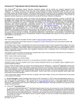
The graphs in Figure 10 show that certain wavelengths
are better suited for fiber optic trans-mission than others.
Selecting the best wavelength for a fiber also depends on the
available light sources and detectors.
10000
Evaluation of these considerations depends on the
application. No single cable will be suited for all applications.
A cross section of an optical cable is shown in Figure 9.
Attenuation (dB/Km)
1000
Strength Member - Material that is added to the cable
to increase tensile strength. Common strengthen-ing materials
are Kevlar, steel and fiber glass strands or rods.
Jacket - The outermost coating of the cable which
provides protection from abrasion, acids, oil, water, etc. The
choice of jacket depends upon the type of protection desired.
The jacket may contain multiple layers.
Jacket
100
Strength
members
400
500
600
700
800
Wavelength (nm)
Buffer
(a)
1200.eps
Cladding
Core
50
1309.eps
Figure 9. Cross-section of an optical cable.
Attenuation (dB/Km)
20
30
40
Typical indoor fiber optic cables include:
• Simplex
• Duplex: Dual channel
• Multifiber
• Plenum-duty
• Undercarpet
10
Examples of outdoor cable:
• Overhead: Cables strung from poles
• Direct Burial: Cables buried in a trench
• Indirect Burial: Cable located underground inside
conduit.
• Submarine: Underwater cable
500
600
700
800
900
1000
1100
Wavelength (nm)
(b)
Figure 10. Attenuation of glass fiber (a), plastic fiber (b).
Fiber Materials
The most common materials for making optical fibers are
glass and plastic. Glass has superior optical qualities, but is
more expensive per unit volume than plastic. Glass is used
for high data rates and long distance transmission. For lower
data rates over short distances, plastic fibers are more
economical. A compromise option is plastic-clad glass fiber.
The fiber core is high quality glass with an inexpensive plastic
cladding.
Attenuation of an optical fiber is very dependent on the
fiber core material and the wavelength of operation.
Attenuation of a glass fiber (a) and of a plastic fiber (b) is
shown in Figure 10.
- 10 -
LIGHT SOURCES & THEIR CHARACTERISTICS
This section covers fiber optic light sources, those
elements which emit light that can be directed into fiber cables.
The rest of the transmitter will be discussed in the next
section.
Two types of fiber optic sources supply greater than 95
percent of the communications market: light emitting diodes
(LEDs) and laser diodes. (In industrial applications there may
be other sources, but these will be covered in the section on
industrial applications.) Both sources are made from
semiconductor material and technology.
Both of these emitters are created from layers of p- and ntype semiconductor material, creating a junction. Applying a
small voltage across the junction causes electrical current to
flow, consisting of electrons and holes. Light photons are
emitted from the junction when the electrons and holes
combine inside the junction.
The best LED or laser for a fiber optic system is
determined by several criteria:
• Output power
• Wavelength
• Speed
• Emission pattern
• Lifetime and reliability
• Drive current
Table 2. Typical characteristics of LEDs and
lasers.
Characteristics
LED
Laser
Spectral width
20-60 nm
0.5-6 nm
Current
50 mA
150 mA
Output power
5 mW
100 mW
NA
0.4
0.25
Speed
100 MHz
2 GHz
Lifetime
10,000 hrs
50,000 hrs
Cost
$1.00-1500
$100-10 k
LED
LEDs are the simplest of the two sources and the most
widely used in fiber optic systems for the following reasons:
• Sturdy
• Inexpensive
• Low input power
• Very long life expectancy
LEDs are made from a variety of materials. Color or
emission wavelength depends upon the material. Table 3
shows some common LED materials, with corresponding
colors and peak wavelengths.
Simple LEDs emit light in every direction and are
constructed to optimize light coming from a particular surface.
There are two types of LEDs, or packaging schemes for p-n
junctions: surface-emitting LEDs and edge-emitting LEDs.
Surface-emitting LEDs
This is the most common LED packaging type. It is used
in most of the visible LEDs and displays. Surface emitters are
the easiest and cheapest to make. Figure 11(a) depicts typical
surface emitter construction and a typical emission pattern.
Edge-emitting LED
The edge emitter, as shown in Figure 11(b), emits all of
its light parallel to the p-n junction. The emission area is a
stripe and the emission forms an elliptical beam. Edge-emitters
can direct much more light into small fibers than do surface
emitters. Because of the high price of fabricating edge-emitting
LEDs there are very few being manufactured today. They are as
expensive to make as laser diodes and more as compared to
the laser diodes manufactured for CD players.
Table 3. Common materials used to make LEDs and laser diodes and their output characteristics.
Material
Color
Wavelength
Gallium phosphide
green
560 nm
Gallium arsenic phosphide
yellow-red
570-700 nm
Gallium aluminum arsenide
near-infrared
800-900 nm
Gallium arsenide
near-infrared
930 nm
Indium gallium arsenic phosphide
near-infrared
1300-1500 nm
- 11 -
simultaneously occur. The very complex fabrication process
causes laser diodes to be higher priced than surface-emitting
LEDs.
Power
Emitting
Junction
Figure 11. (a) Surface-emitting LED. (b) Edge-emitting LED.
In general, the output power of sources decreases in the
following order: laser diodes, edge-emitting LEDs, surface
emitting LEDs. Figure 12 shows some curves of relative
output power versus input current for LEDs and lasers.
Optical power (relative)
1450.eps
Both LEDs and lasers have voltage versus current curves
similar to those of regular silicon diodes. The typical forward
voltage drop across LEDs and laser diodes, made from Gallium
Arsenid, is 1.7 volts.
Laser
LED
Lasers
Laser is an acronym for light amplification by stimulated
emission of radiation. The main difference between an LED
and a laser is that a laser has an optical cavity, which is
required for lasing. This cavity is called a Fabry-Perot cavity. It
is formed by cleaving the opposite ends of the edge-emitting
chip to form highly parallel, reflective mirror-like finishes.
At low electrical drive current lasers act as LEDs. As the
drive current increases, it reaches a threshold, above which
lasing occurs. A laser diode relies on a very high current density
to stimulate lasing. At high current densities, many electrons
are in the excited state. As in LEDs, holes and electrons
combine inside the laser, creating photons, which are confined
to the optical cavity. Photons can travel only along the length
of the optical cavity, and as they travel they collide with other
electrons, generating new photons. These photons are clones
of the first photons; they travel the same direction, have the
same phase and wavelength. The first light photon amplified
itself by stimulating an electron to emit another photon.
Current (relative)
1281.eps
Figure 12. Output optical power versus current for LEDs and
laser diodes.
Wavelength
Because optical fibers are sensitive to wavelength, the
spectral (optical) frequency of the fiber optic source is
important. Lasers and LEDs do not emit a single wavelength;
they emit a range of wavelengths. The spectral width is the
optical bandwidth at which the intensity of emission falls to 50
percent of the peak —sometimes known as full width half
maximum [FWHM]. The spectral width of a laser is 0.5 to 6
nm; the width of LEDs is several times wider, typically
between 20 and 60 nm.
Both ends of the laser diode can be 100 percent reflective
or there would be no optical output. Usually, one end has a
partially reflecting facet to allow some optical power to escape
to be used in fiber optic systems.
The stimulated emission process is very fast; laser diodes
have been modulated at up to 16 gigabits per second.
Producing a laser diode is much more difficult than the
simple description just given. Many material properties must all
- 12 -
Speed
Safety
A light source must turn on and off fast enough to meet
the bandwidth requirements of the fiber optic system. Source
speeds are specified by rise and fall times. Laser diodes have
rise time less than 1 nanosecond, whereas LEDs have slower
rise times, typically 5 nanoseconds or greater. A rough
approximation of bandwidth of a device, given the rise time, is
Light from lasers or other light sources can cause eye
damage just as directly looking at the sun can. Particularly with
fiber optics systems, the light is infrared and not visible to the
eye. Infrared radiation can be very dangerous because the
normal human blink response will not protect the eye, nor can
it be visibly seen.
!
w
where
!
w
=
0.35
t
Equation 10
r
is bandwidth in Hz and
t
r
is rise time in seconds.
Lifetime
The expected operating lifetime of a source can run into
thousands of hours. Over time, the output power decreases
due to increasing internal defects. The specified lifetime of a
source is the time for the output power to decrease to 50
percent of initial value. LEDs have a much longer lifetime than
lasers. The conditions under which lasing occurs cause greater
thermal stress, promoting growth of internal defects in the
device, decreasing longevity.
Usage
Although a laser provides better optical performance than
an LED, it is also more expensive, less reliable and harder to
use. Lasers often require more complex electrical driving
circuits. For example, the output power of a laser changes
significantly with temperature. Therefore, to maintain proper
output levels and prevent damage to the laser, special circuitry
is needed to detect changes in temperature or optical output
and adjust the electrical drive current according to temperature
or output power.
Generally, light from LEDs is not intense enough to cause
eye damage, but the emission from laser diodes can be
harmful. Users should be especially conscious of collimated
light beams from LEDs or lasers.
Because most fiber optic communications systems have
very low optical power, eye safety is not usually a problem, but
do not take it for granted. If you do not know, ask! The
precautions are simple:
• Do not look directly into an LED or laser diode
• Avoid all eye contact with all collimated
beams
• Before working with fiber optics
familiar with pertinent safety standards
become
For more information about safety, contact the Laser
Society of America or OSHA. See section titled References for
safety information.
- 13 -
TRANSMITTER COMPONENTS
The light source is the most important component of a
transmitter, but it is not sufficient by itself. A housing is
required to mount and protect the light source and to interface
with the electronic signal source and transmitting optical fiber.
Internal components may be necessary to optimize light
coupling into the optical fiber. Electrical drive circuitry is needed
and output monitoring may be crucial for sophisticated laser
diodes.
Practical boundaries between
transmitters and light
sources can be vague. Simple LED sources can be mounted in
a case with optical and electronic connections, with little or no
drive circuitry. On the other hand, a high-performance laser
may be packaged as a transmitter in a case that also houses an
output monitor and thermoelectric cooler.
Housing
The simplest housing for a fiber optic transmitter is an
adequately sized box that can be conveniently mounted with
screws or other means to a printed wiring board or other
electrical interface. Some transmitters are built inside a
mechanical box, with only electrical and optical connections
exposed.
Electronic Interface
Electronic interfaces can be wires, pins, or standard
electrical connections. Transmitters containing a LED may only
have two simple electrical connections. Others may be more
complex, requiring electrical power, feedback interfaces
resulting in circuits and up to 16 or more interconnects.
Elements of a Transmitter
Drive Circuits
The basic elements commonly found in transmitters and
shown in Figure 13 are:
• Housing
• Electronic interface
• Electronic preprocessing
• Drive circuits
• Light sources
• Optical interface
• Temperature sensing and control
• Optical monitor
The type of drive circuit depends upon the application
requirements, data format and light source. LEDs are best
driven by a current source. (Most electronic signals are voltages
and must be converted to current.) Some LEDs work better
with special drive circuitry to tailor the electric current input.
For example, the proper drive waveform can effectively reduce
the rise time of an inexpensive LED and allow its use at higherthan-specified bandwidths.
1353.eps
Semiconductor lasers are generally pre-biased at a current
level near lasing threshold.
Optical
Monitoring
Electrical Interface
Optical Interface
Fiber
Light
Source
Drive Circuits
Temperature
Monitoring
Thermal Electric
Cooler
Housing
Figure 13. Block diagram of elements commonly found in a fiber optic transmitter.
- 14 -
Light Source
Fiber optic light sources are either LEDs or laser diodes.
We discussed these two components in the previous section.
Optical Interface
In most cases, fiber optic system engineers do not design
their own transmitters, but rather use completed assemblies.
For information on Industrial Fiber Optics transmitter
components, please see our Web site at
www.i-fiberoptics.com
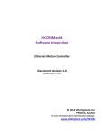
The two forms of optical interfaces are the fiber optic
connector as shown in Figure 14, and a short fiber optic
pigtail coupled to the light source and brought outside the
housing. The pigtail can be spliced or connected to an external
fiber.
Temperature Sensing and Control
These circuits are primarily found in transmitters with laser
diodes, because their output is very temperature-dependent. A
temperature sensing element senses the device temperature,
compares it to a reference, and then adapts the electric heat
pump to control the laser diode temperature. (The most
common heat pump is the thermal electric [TE] cooler.)
Stabilizing the temperature of laser diodes has the additional
benefit of increasing their reliability and lifetime.
Figure 14. Fiber optic FDDI transceiver.
Optical Monitor
Some transmitters include optical output stabilization
circuits. Such circuits sample a small amount of optical energy
with a photodetector and convert it to an electrical signal. The
signal is then used to adjust input drive current, stabilizing
output power.
Requirements
No single fiber optic transmitter will fulfill all the needs of
the many fiber optic designs. There are just too many options
that must be considered when making a design. Following is a
list of important design criteria to consider when selecting a
fiber optic transmitter:
• Modulation type
• Speed
• Output power
• Optical interface
• Electronic interface
• Housing
• Cost
- 15 -
DETECTORS FOR FIBER OPTIC RECEIVERS
In a receiver, the detector is comparable to the light source
in the transmitter. The detector performs the reciprocal
function of the source, converting optical energy to electrical
current. This section will cover the types of semi-conductor
photodetectors.
Table 5. Characteristics of fiber optic detectors.
Fiber optic detectors are fabricated from semiconductor
materials similar to those found in LEDs and lasers.
Device
Responsivity
Rise time
Phototransistor
18 A/W
2.5 us
Photodarlington
500 A/W
40 us
PIN photodiode
0.6 A/W
1 ns
Avalanche photodiode
60 A/W
1 ns
Table 4. Photodetector materials and active regions.
Photodiode
Wavelength (nm)
Silicon
400 - 1050
Germanium
600 - 1600
Gallium arsenide
800 - 1000
Indium gallium arsenide
1000 - 1700
Indium arsenic phosphide
1100 - 1600
A circuit using a semiconductor photodetector is shown in
Figure 15. The diode is reverse biased; little or no current
flows in the absence of light. When light photons strike the
detector, they create hole/electron pairs, causing current flow.
The number of electron/hole pairs (current) is directly
proportional to the amount of light incident upon the detector.
This type of photodetector is called a photoconductive
detector.
There are several types of photodiodes, also. The one
most useful for fiber optics is the PIN photodiode. The name
of the photodiode comes from the layering — positive,
intrinsic, negative — PIN. See the cross-section shown in
Figure 16.
The PIN photodiode has higher efficiency and a faster rise
time than other photodiodes. In a PIN photodiode, one
photon creates one hole/electron pair.
Light
Detector
Aperture
1309.eps
Material
Top Contact
p Layer
Vbias
Intrinsic
Layer
Vsignal
ct
nta
n layer
m
tto
Bo
Co
Figure 16. Cross-section of a PIN photodiode.
1282.eps
Figure 15. Circuit using an optical photodetector.
Types
The characteristics of four types of photoconductive
photodetectors are listed in Table 5. The phototransistor and
photodarlington have little use in most fiber optic systems due
to their slow rise times. Photodiodes and avalanche
photodiodes are the primary detectors for fiber optics.
Avalanche Photodiode (APD)
The avalanche photodiode is similar to the laser diode. In
a laser, a few primary carriers result in many emitted photons.
In an avalanche photodiode, a few photons produce many
carriers.
When an avalanche photodetector absorbs a photon, it
creates a hole/electron pair in the intrinsic region. The APD is
reversed biased, causing the holes and electrons to move in the
electric field. In an avalanche photodiode this electric field is
much stronger than in a PIN diode, due to higher bias voltage
(typically 100 – 400 volts). The holes/electron pairs accelerate
while traveling in this strong electric field. These pairs collide
with electrons/holes, generating another set of carriers, i.e.,
avalanching.
- 16 -
The avalanche process amplifies the number of carriers
generated from a single photon. Typical magnifications are 10
to 100.
Avalanche photodiodes are used in fiber optic systems
because the system noise level is limited by the interface
electronics which follow. The avalanche photodiode provides
pre-electronics gain.
Disadvantages of using avalanche photodiodes:
Gain variation with temperature
High voltage power supply required
Power dissipation
Higher price
Responsivity
A fiber optic system's bandwidth is very dependent on the
photodetector bandwidth or rise time. Equation 10 applies to
detectors as well. Rise time is furnished on the manufacturer's
data sheets. Rise times can be dependent on the bias voltage
applied to the photodetector. The rise and fall times are very
comparable in PIN photodetectors and avalanche photodiodes.
Bias Voltage
Both photodiodes and avalanche photodiodes are reverse
biased. Typical bias voltage for photodiodes is 5 to 100 volts.
Photodiodes operating with a low bias voltage will have more
internal capacitance which slows down rise and fall times.
Avalanche photodiodes require a much higher voltage,
typically 100 to 400 volts. The bias voltage of avalanche
photodiodes determines the responsivity of the device, as
shown in Figure 18.
1361.eps
Responsivity (A/W)
40
60
80
20
200
Rise time
100
1284.eps
Responsivity Relative %
40
60
80
100
The responsivity of a detector is a measure of its
efficiency. A good detector has an efficiency between 80 and
85 percent. A plot of silicon PIN photodiode responsivity
versus wavelength is shown in Figure 17. The shape of the
response is typical and consistent with solid state theory. It is
beyond the depth of this course to discuss this, but suffice to
say that a 100 percent efficient detector does not generate 1
Amp per watt. The typical responsivity of a silicon PIN diode
is .6 A/W.
Dark current is the current flowing through a detector in
the absence of any light when in an operational circuit. This
value is normally specified on the manufacturer’s device data
sheets as a worst-case condition at a given temperature. The
dark current in silicon PIN photodiodes or APDs doubles every
10° C.
400
600
nm
800
1000
1200
20
•
•
•
•
Dark Current
Figure 17. Responsivity of a silicon photodiode versus
wavelength.
150
The shape of the curve shown in figure 17 is dependant upon
the detector material. Above a certain wavelength, light
photons will not contain enough energy to create a
hole/electron pair (see Equation 2). This explains the sharp
roll-off to the right of the peak. For the curve left of the peak,
remember that if the optical power remains constant, the
number of photons (per watt of energy) decreases as the
wavelength gets shorter. In a detector each photon creates one
hole/electron pair, thus the responsivity decreases with
wavelength with constant energy. The remainder of the energy
is converted to heat. Other effects also occur below 500 nm,
but this is outside fiber optic normal operating regions.
200
250
300
350 volts
Figure 18. Responsivity versus voltage for an APD.
- 17 -
ELEMENTS OF FIBER OPTIC RECEIVERS
Preamplifier
The preamplifier sets the two most important
performance levels in a fiber optic system: minimal detectable
signal and electrical bandwidth. At the preamplifier, the signal is
the weakest and the most susceptible to extraneous sources.
Typical input-current levels to preamplifier are 0.1- 100 µA.
The receiver is as essential an element of any fiber optic
system as the fiber or light source. The receiver converts the
optical signal transmitted through the optical fiber to an
electrical form. Again, the boundary between receivers and
detectors is variable, depending on the system requirements.
The transfer function of a fiber optic preamplifier has the
dimensions of volts per Amp. (Most electronic amplifiers have
transfer functions of volts/volt.) This unusual dimension of
these preamplifiers gives them an alternate name,
transimpedance amplifiers.
Receiver Elements
Fiber optic receivers come in many varieties, from simple
packaged photodetectors to sophisticated systems for high
speed transmission. The description of a receiver is a little
more complicated than the transmitter because there are two
types of receivers, analog and digital. The basic elements of all
receivers are:
• Housing
• Electronic interface
• Optical interface
• Detector
• Low-noise preamplifier
• Main amplifier
• Signal processor
Main Amplifier
The main amplifier further amplifies the transimpedance
amplifier signals to higher levels. Typical values would be 0.7
to 3.4 volts in a digital TTL system. In an analog system, the
main amplifier could be a power amplifier for driving a 50 ohm
load
1351.eps
The information pertaining to the housing, electronic
interface, and optical interface covered in the section on
transmitters applies equally to receivers.
Optical Interface
Photodetector
Preamplifier
Main
Amplifiier
Fiber
Electrical Interface
Signal
Processor
Housing
Figure 19. Typical elements of a fiber optic receiver.
- 18 -
Data
Output
Noise in Fiber Optic Receivers
The detector, preamplifier, and main amplifier are the
same for both analog and digital receivers, but the signal
processors are different. See Figure 20.
Every component in a fiber optic receiver generates
electrical noise. This noise has a Gaussian distribution. The
amplitude depends on the receiver bandwidth and associated
components, but the detector and preamplifier are the major
sources.
From
Main
Amplifier
Demodulator
1285.eps
Signal Processor
Analog
Output
Analog processor
The noise current generated in a photodiode is called shot
noise. It can be calculated by Equation 11,
2
s
i
Shaping Filter
Decision
Circuit
Digital
Output
Timing
1286.eps
From
Main
Amplifier
Requirements
Fiber optic receiver requirements are so different that a
single device cannot fit every need. Besides selecting between
analog and digital receivers, there are many other options.
Following is a list of the more important features in a receiver:
• Modulation
• Bandwidth
• Noise
• Dynamic range
• Optical interface
• Electronic interface
• Housing
• Cost
Fiber optic engineers, in most cases, do not design their
own receivers, but rather use completed assemblies. Details of
receiver design will be left to more advanced classes, but a
brief discussion of the two most critical receiver parameters
follows.
Equation 11
in which e is the charge of an electron, 1.6 X 10-19 coulombs,
! is system electrical bandwidth in Hz, and I is the dc
current flowing through photodiode in amps.
Shot noise generation is due to the statistical nature of
electron flow across the p-n junction.
Thermal noise or Johnson noise is caused by noise
generated in resistors and electronics, and can be calculated
from Equation 12.
Digital processor
Figure 20. Analog and digital fiber optic receiver signal
processors.
=2 e I !
2
th
i
4 ! "#
Req
=
Equation 12
! is Boltzman's Constant (1.38 E-23 joules/° K), T is
the absolute temperature (oKelvin) and Req is the equivalent
resistance of the transimpedance amplifier.
The total noise current of a photodiode and preamplifier
can be summed up by Equation 13.
2
noise
i
=
2
shot
i
2
+ ith
Equation 13
Receiver Bandwidth
The electrical bandwidth of most fiber optic receivers is
set by the preamplifier. Generally, photodiodes and avalanche
photodiodes with wide bandwidths are easier to find than wide
bandwidth, low-noise preamplifiers.
The fiber optic receiver in Figure 19 has a series of
elements that each can reduce system bandwidth or rise time.
Calculation of overall system rise time can be done with
Equation 14. Bandwidth can be computed with Equation 10.
Equation 14
t ( system) = (t (transmitter ) + t
+ t ( preamp) + ...)
2
r
r
2
r
- 19 -
0.5
2
r
(det ector)
PASSIVE OPTICAL INTERCONNECTIONS
Interconnecting the various components of a fiber optic
system is a vital part of system performance. This section
discusses the mechanics and requirements for fiber optic
connections and distribution. The three most important
interconnects involve connectors, splices and couplers.
The losses in a fiber optic interconnect can be separated
into two categories.
Intrinsic, or fiber-related, losses caused by variations in
the fiber itself, such as numerical aperture mismatch,
concentricity, ellipticity and core/cladding mismatches.
Extrinsic, or interface-related, factors contributed by the
interface itself. The main causes of these losses are lateral
displacement, end separation, angular misalignment and
surface roughness.
Connectors
The fiber optic connector is a non-permanent
disconnectable device used to connect a fiber to a source,
detector, or another fiber. It is designed to be easily
connected and disconnected repeatedly. Listed below are
some of the desirable features in a connector:
• Low loss
• Easy installation
• Repeatability (low variations in loss after
disconnection)
• Consistency (between connectors)
• Economical
It is very difficult to design a connector to meet every
requirement. A low-loss connector may be more expensive,
take longer to install, or require high-priced tooling than a
higher-loss connector.
•
•
•
•
NA mismatch
The many different kinds of connectors include:
SMA
ST
Bi-conic
LC
Core diameter mismatch
Lateral displacement
Cladding diameter mismatch
Core 1
End separation
Cladding
Core 2
Core(s)
Concentricity
Ellipticity
Angular misalignment
1287.eps
1288.eps
Figure 21. Intrinsic fiber optic losses.
Figure 22. Extrinsic fiber optic losses.
- 20 -
The SMA fiber optic connector is the oldest type of
connector, evolving from the SMA electrical interface. The
ST, Bi-conic and LC are connectors recently designed
specifically for fiber cable using small core fiber, having low
loss and meeting environmental considerations.
a carefully made fusion splice can withstand roughly the same
stress as an unspliced fiber. Wire splices will nearly always fail
in the joint.
The installation of a fiber optic connector is similar to
that of electrical connectors, but it does require more care,
special tools and little more time. The steps in making a fiber
optic connection are outlined below:
• Open cable
• Remove jacketing and buffer layers to expose fiber
• Insert fiber cable into connector
• Attach connector to fiber with crimp or epoxy
• Scripe fiber
• Polish or smooth the fiber end
• Inspect fiber ends with microscope
The fusion splice, the most common fiber splice, is
formed by heating two ends of fiber and welding them
together.
Splices
Unlike connectors, splices are a permanent connection
between two fibers. Table 6 presents a comparison of
connectors and splices.
The main concerns in a fiber optic splice are:
• Losses in splice
• Physical durability
• Ease of making splice
The losses in a fiber optic splice are identical to those in
a connector — intrinsic and extrinsic. However, the methods
used to make fiber optic splices produce tighter tolerances,
and therefore lower attenuation. Some sources of loss are
reduced; others are eliminated.
Fusion Splices
A splice begins with cleaving the ends of both fibers. (A
fiber cleave is made by scribing or nicking the fiber and
putting it under tension by pulling or bending. This causes
the fiber to break along the crystalline structure. Ideal cleaves
are perfect — no discontinuities.) The ends are cleaned and
prepared with a preform electrical arc, then the fibers are
aligned with micropositioners and a microscope or an
automatic alignment processor. A final fusion completes the
splice process. The electrical arc raises the fiber temperature
to 2000° C, melting the glass. Time duration and energy in
the arcs can be controlled, which allows optimal splices for
many different types of fibers.
Mechanical Splice
Mechanical splices join two fiber ends by clamping them
within a structure or by gluing them together. Because
tolerances in mechanical splices are looser than fusion
splicing, this approach is used more often with multimode
than single-mode fiber. Mechanical splices are easy to
perform and do not require expensive splicing equipment.
Losses are generally higher in mechanical splices than in
fusion splices.
Because most fiber optic splices are made in the field, the
ease with which splices can be made is very important. This
has led to development of very specialized fiber splices and
equipment.
A splice is made by either fusing (melting), gluing, or
mechanically holding two fibers together. Unlike wire splices,
Table 6. Comparison of fiber optic connectors and splices.
Connectors
Splices
Non-permanent
Permanent
Factory installable on cables
Easier to get low loss in field
Easy reconfiguration
Lower attenuation
Simple to use
Spliced fibers can fit inside conduit
Field installable
Some are hermetically sealed
Less expensive per interconnect
Stronger junction
- 21 -
Couplers
The term "coupler" has a special meaning in fiber optics. A
fiber optic coupler connects three or more fibers. As such, it is
distinct from connectors and splices, which join only two
entities. In fact, splices or connectors link fibers to couplers.
The coupler is far more important in fiber optics than in
electrical signal transmission because the way in which optical
fibers transmit light makes it a problem to connect more than
two points. Fiber optic splitters, or couplers, were developed
to solve that problem.
Important issues in the selection of a coupler include:
• Number of input and output ports
• Type of fiber (single or multimode)
• Sensitivity to direction
• Wavelength selectivity
• Cost
For fiber optic users, couplers are "black boxes". Normally
these are purchased, like transmitters and receivers. The use of
couplers is quite simple and only a couple of terms need to be
defined.
Excess loss - The optical loss inside the coupler,
determined by dividing the sum of all the output power by the
input power. Normally expressed in dBs
Insertion loss - The reduction of optical power occurring
within an optical coupler due to light transmitted from any
input to an output fiber in a coupler. It is usually specified as a
maximum value and in dBs. (This term can be used to
determine quickly the minimum optical power at any fiber
output if the input power is known.)
T coupler
The two types of passive couplers are the "star" and the
"T", shown in Figure 23. The T coupler has three ports, as the
name would suggest. The star coupler can have multiple input
and output ports, and the number of input and output fibers
does not have to be the same.
1
1
MXN
M
1289.eps
N
Figure 23. The "T" and "star" fiber optic couplers.
- 22 -
FIBER OPTIC SYSTEM DESIGN & ANALYSIS
Many of the variables above are interrelated, e.g.,
transmitter power depends on the source. Most systems will
require a compromise between several variables — and a highly
reliable system may not be inexpensive.
S/N Ratio and Bit Error Rate
Fiber optic transmission is very similar to electrical data
transmission. The real world clutters up the data with
randomly generated noise and attenuates the signal over
distance. The data "quality" is usually referred to as
where isignal is the signal input to the amplifier and
noise current in the receiver.
i
the
noise
15
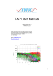
Bit error rate is a function of signal-to-noise ratio, data
format, and error-correcting schemes. Figure 24 is a plot of
BER versus signal-to-noise ratios for a simple non-errorcorrecting data transmission. A typical BER for telecommunications is 10-9, or one error in 1 billion data points.
Computer data interfaces typically operate with BERs of 10-12.
14
1290.eps
With the distance and data rate established, secondary
features can now be considered, such as those shown below.
Those features with asterisks after them should be furnished
as part of the system specification or requirement.
Type of fiber: single or multimode
Fiber numerical aperture
Fiber core diameter
Operating wavelength
Fiber attenuation
Fiber dispersion
Source type: LED or laser
Transmitter power
Detector type: PIN diode or APD
Receiver sensitivity
Bandwidth of receiver and transmitter
Signal-to-noise ratios / bit error rate
Connector losses and number
Splice losses and number
Environmental concerns *
Mechanical concerns *
Reliability *
Cost *
Equation 15
Signal/Noise (dB)
11
12
13
The first step in planning a fiber optic system is to define
the applications requirements. The main issues are: How far?
How fast? The answers to these basic questions determine
the system hardware to a large extent.
" i 2signal %
S
= 10 • Log$$ 2 ''
!
# i noise &
10
Design Criteria
Signal-to-noise is the ratio of signal power to noise power
in the receiver. Signal-to-noise ratio is commonly expressed in
dBs.
9
We have looked at the main components of a fiber optic
link including cables, light sources and transmitters, optical
detectors and receivers, and connectors and couplers. This
section will bring all of that information together to show you
how to analyze and specify a fiber optic link. The two main
considerations for all fiber optic systems are the optical power
and system bandwidth budgets.
10-12
10-10
10-8
Bit error rate
10-6
Figure 24. BER versus signal-to-noise ratio.
Signal-to-noise ratio or BER is usually specified by the
communications system or engineer. This parameter must be
specified or agreed on before system design can begin.
System Margin
One quantity that should always be entered into a fiber
optic system is safety factor, or design margin for the system
designer. This allows for uncertainties in counting the losses
and for system degradations, such as output of light sources
decreasing over time, a spliced broken cable, increased
attenuation due to moisture, or receiver becoming less
sensitive. Typical margins are 1 to 4 dB.
Signal-to-Noise ratio (S/N) for analog signals, and Bit Error
Rate (BER) for digital signals.
- 23 -
Analyzing the System
Table 7. Guide to fiber selection.
Drawing a diagram showing all interconnections and
interfaces is the first step in designing and analyzing a fiber
optic system. See Figure 25. Distances and bandwidths can be
included, but are not required.
Connector
Receiver
Connector
Step index
Graded
index
Single
mode
Bandwidth
Moderate
High
Very high
Short to
Medium to
Very long
medium
long
Distance
Remember, an LED is always the cheapest and the easiest
to use. An alternative to using a laser diode transmitter is to
use a more sensitive receiver, one with an APD.
Splice
1291.eps
Transmitter
Interfaces
Fiber type
2 km length
of fiber
Figure 25. System design diagram.
Component Selection
The next step is to choose the fiber type and the source.
Table 7 will help select the fiber. For long distances or high
bandwidths, a laser diode must be used. For moderate
bandwidths and short distances, an LED can be used. For
conditions in between, the particular system lengths need to be
detailed.
Check to see if the fiber choice and source will meet the
system bandwidth requirements from the standpoint of
dispersion characteristics of fiber and spectral width of source.
!
modal
A selection of fiber optic cable must now be made, as this
will drive the remainder of the system design. The
environmental and installation procedures will determine the
type of cable.
The choice of connector and splices will be made based
on the fiber type. The Buying Guide is a valuable resource here
also. See References.
!
system
Equation 16
On the "system design diagram", estimate loss at all splices
and connectors. (A decision on connectors has not been made
yet, but this is a first cut.) Losses due to splices range from .1
to 1 dB and for connectors, .5 to 3 dB.
The next step is to calculate the receiver sensitivity
required for the system. We will use the digital system shown
in Figure 25 as an example. Using the log scale allows
addition, rather than multiplication, of losses.
Loop loss budgets require the electrical S/N ratio to be
divided by 2. From the analysis above, a receiver with an NEP
of 4 µwatts must be used. This is typical for a detector with a
PIN diode. The selection of the type of detector has now been
made.
The next step is to locate the parts that have been
identified so far: transmitter, receiver, and cable. For the
inexperienced designer, the Fiberoptic Product News "Buying
Guide" is an excellent source of information about vendors and
all fiber optic components. See References.
>
Transmitter Power
Transmitter Losses
Connector
Splice
Connector 2
Fiber Attenuation 2 dB/km
Receiver Losses
Design Margin
S/N Ratio BER
-12
-1
-2
-.05
-2
-4
-1
-4
-10
dBm
dB
dB
dB
dB
dB
dB
dB
dB
Minimum Receiver Sensitivity
-36.5 dBm
All the specifications on the previous page should now be
complete. If not, review what has been missed and seek out
that information. Very often, the first design is too costly or
some other requirement is missed. Now it’s time to do
another review of the design. (One method that works quite
well is putting the system loop loss on a computer
spreadsheet. In the first column show the description of the
loss and in column two the value. This provides an index for
the value and a description at the same time.) Update the
loop loss budget each time. You should be getting closer to
meeting all the specifications after each design review.
- 24 -
FIBER OPTIC TEST EQUIPMENT & TOOLS
This chapter will take a brief look at some of the tools
used to characterize and inspect a fiber optic system. The
equipment covered will include an optical power meter, optical
time domain reflectometer, fiber cleaver, fusion splicer,
polishing machine, microscope and hand tools.
Optical Power Meter
The optical power meter is analogous to the volt-ohm-amp
meter used in electronics. Most meters can read optical power
either in watts or dBm.
The meter itself is completely electronic. Modules plug
into the meter which contains an optical detector that converts
the input optical energy to electrical current. (This module is
essentially a calibrated receiver.)
Different modules are
available for a variety of wavelengths and power levels.
Adapters permit testing bare fibers or different connectors.
The optical power meter can be used for a variety of
measurements such as fiber attenuation, losses in connectors
and splice losses.
Directional
Coupler
Optical Time Domain Reflectometer
(OTDR)
An OTDR is a tool similar to an oscilloscope. As the
name implies, the optical time domain reflectometer allows
evaluation of an optical fiber in the time domain. Useful for
testing fiber cable, it provides the user a picture of what is
happening along the fiber length.
Figure 26 shows a simple block diagram of an OTDR. A
short, high-power pulse is injected into the fiber through a
directional coupler. This light travels through the optical fiber,
with portions of light scattering backwards due to
imperfections or reflections. The return power is directed into
the photodetector by the directional coupler and amplified by a
receiver. The OTDR displays the returned optical power and
the time (distance) on the vertical and horizontal axes
respectively. See Figure 27.
Breaks in fibers can be determined by the high magnitude
of backscatter due to Fresnel reflections. The location is found
by knowing the refractive index of the fiber, reading the time
from the OTDR, and calculating the distance. Remember that
the time show on the OTDR is the time for two-way travel.
Collimating
Lens
Pulsed
Light
Source
High-speed
Photo
Detector
Amplifier
Vertical Input
Sweep Trigger
Figure 26. Block diagram of OTDR.
- 25 -
Oscilloscope
1292.eps
Pulse
Generator
Fiber
The fusion splicer is a very sophisticated tool specifically
developed for fiber optics. It has no counterpart in electronics.
A fusion splicer is available with many options including a
fusion welder, positioning mechanisms for fiber, optical power
and a fiber cleaver. The optical power meter
checks
transmission before and after splicing.
Reflected power ( dB )
Launch
pulse
Splice reflection
Connector reflection
End
of
fiber
Time
1298.eps
Figure 27. Typical display from an OTDR.
Power Meter
Power meters are a fundamental piece of equipment used
in fiber optics, much as a voltmeter is used in electronics.
Power meters measure optical energy coming out of a fiber,
transmitter, repeater, or other optoelectronic devices used in a
fiber optic system. They often are similar in appearance to the
digital voltmeters used in electronics; however, they measure
optical power in units of watts or dBm. Power meters consist
of a photodetector (and appropriate input connector) and a
read-out device to measure the light-induced current from the
detector. A power meter can be used to measure the total
quantity of optical power coming from a fiber or transmitter,
and when properly configured, the attenuation or loss through
fiber cables and connectors. Figure 28 is of a power meter
designed for use with plastic optical fiber.
Figure 29. Fusion splice for glass optical fiber
Polishing Machine
The polishing machine partially automates the polishing of
fiber optic connectors to produce faster and more consistent
end finishes. Machines can contain one or more polishing
wheels. Some machines polish only one connector at a time,
while others can handle 32 or more. Polishing time ranges
from 30 seconds to five minutes.
Microscope
Microscopes are used for close-up inspection of cleaved
fiber ends and connector polishes. They are available in either
laboratory or portable field models.
Installation Kits
Figure 28. Optical power meter with a built-in light source.
Fiber Cleaver
The fiber cleaver is a special tool for cutting a glass core
fiber. (Glass fibers are really cleaved, since cutting would result
in a very poor termination.) Plastic fibers can be cut using any
sharp blade, but glass fibers are cleaved by scribing with a
diamond or carbide tipped tool. This weakens the fiber,
causing it to cleave when bent or stressed. Special jigs or parts
of the cleaver are made to cause the fiber to break as close to
perpendicular as possible.
The installation of fiber cable and connectors requires
special tools used only in fiber optics. Often these tools are
purchased as a kit for a particular fiber or connector type.
Choosing a different connector may require additional tools.
(One of the reasons fiber optics achieves such high
performance is because of the specialized tools and connector
systems.) Special tools commonly found in a fiber optic tool
kit may include:
Cable stripper for removing jacketing
Scissors for cutting strengthening members
Fiber stripper for removing buffer coating
Scribe tool for cleaving fibers
Crimp tool for crimping connector to fiber
Polishing fixture and materials
Heat gun for heat shrink tubing
Epoxy
Index-matching fluid
Inspection microscope
Fusion Splicer
- 26 -
INDUSTRIAL APPLICATIONS OF FIBER OPTICS
Fiber optics is used for many applications besides data
communications. Every day, non-communication uses of fiber
optics affect our lives and we may not even know it. Are the
indicators in the “walk sign” for the crosswalk really individual
lights? The light in the ashtray of your automobile? The
security alarm in your office? These are some of the more
common applications of fiber optics that we seldom notice.
Numerous applications of fiber optics are not widely
publicized.
Communication was a latecomer in the world of fiber
optics. Early developers had other things in mind. Uses have
included imaging, sensing, medical and lens design.
Other Fiber Optic Technologies
GRIN-Lenses
GRIN is an acronym for graded index of refraction. The
development of graded-index multimode fiber led to the
concept of GRIN lenses.
Review the travel light in graded-index fiber shown in
Figure 7 (a). Imagine a section of that fiber being used as a
lens. Look at a single ray traveling through a short section of
the fiber. The grade index refracts the light rays in that they are
constantly changing as the light travels. If a section of fiber
was cut after the light had gone through 90° or 270°, the fiber
would act as a collimation lens.
A lens which has only 90° of refraction is known as a 1/4
pitch GRIN lens. A 1/2 pitch lens could be used to connect a
fiber to a detector.
Detector
Fiber
Interfacing
1364.eps
Light
Source
Collimation
Figure 30. Uses of GRIN lenses.
Practical GRIN lenses are not pieces of graded-index fiber.
They are larger in diameter and have a greater refractive index
profile. This makes them versatile for applications other than
fiber optic interconnects.
Fiber Bundles
The basic principles of fiber optics are the same, whether
the fibers are separated or bundled. Each fiber in the bundle
transfers light from source to receiver. The two types of fiber
bundles are coherent and non-coherent.
Coherent bundles have fibers packaged together in a
bundle, retaining a fixed arrangement at both ends, which can
transmit an image.
Non-coherent bundles have fibers packaged in a random
manner, not retaining a fixed arrangement at the two ends,
which scramble the image.
Fiber bundles can be either flexible or rigid. Generally, all
non-coherent bundles are flexible, while coherent bundles can
be either. Coherent bundles are the easiest to make, if all the
fibers are fused together along the entire length. Rigid fiber
bundles have limited applications because they do not bend.
A flexible coherent fiber bundle is made by bonding or
fusing the fibers together at the ends and maintaining critical
alignment at the image points. This leaves the middle region
free to move. Individual fibers themselves can be bent into
quite small radii, allowing the bundle flexibility. These bundles
are usually housed inside a flexible sheath to protect the fibers.
Individual fibers in a flexible coherent bundle can be quite
small, but not as small as in a fused rigid bundle. The imaging
quality of a bundle is related to the number of fiber cores per
unit area.
With flexible bundles, an individual fiber can break, but
single fiber breaks do not occur in rigid bundles. The loss of a
single fiber is not significant, but if the number increases, the
image is eventually lost. Plastic fibers are often used in flexible
bundles to allow maximum flexibility.
Most fiber optic bundles are made from a high NA, stepindex multimode fiber. Increasing the NA allows for decreased
coupling losses and higher transmission. The typical fiber
bundle's NA ranges from 0.4 to 0.7. Optical dispersion in fiber
bundles is not important.
Fibers used in bundles typically have higher attenuation
than communication fibers, around, say, 1 dB/m. For imaging
and illumination, visible light is used and a broader
transmission band is needed. In some applications, such as
medical, fibers may be used at wavelengths where the
transmission is not the best — for example, sending an ultraviolet laser beam down a glass fiber. Short-distance glass fibers
are usable from 400 to 2000 nm.
Fiber bundles, like single fibers, are not 100 percent core.
Each core is surrounded by cladding. Picture a light source
imaged onto the end of a fiber bundle. Some light falls onto
the cladding. Cladding is not transparent so some transmission
efficiency is lost. This loss is not found in single fibers and
- 27 -
makes part of the bundle's overall efficiency dependent on the
total core area. Collection efficiency depends on the packing
fraction of the bundle defined as:
!acking fraction =
"otal core area
"otal surface area
The closer a bundle's packing fraction ratio is to 1 the
better the coupling efficiency.
Fiber Optic Face Plates
A fiber optic face plate is a very short, rigid fiber optic
bundle. It usually has larger height and width dimensions than
depth. Because the applications are very different, we shall
consider them separately.
The main role of a face plate is to transfer an image from
inside to outside, or vice versa, with as little loss as possible.
A faceplate's resolution is limited to the number of fibers per
unit area.
Faceplates may be used as a window on a CCD display or
a window for an image-intensifier tube. They can be designed
to flatten the curved field of a CRT or, by twisting the fiber
bundle 180°, invert the optical image. Face plates can be
fabricated to function as optical elements in very small,
demanding applications.
Applications
Medical
Coherent fiber optic bundles called "endoscopes"
constitute the most important use of fibers in the medical
field. They can be flexible or rigid, depending on the procedure.
A typical medical procedure might be to examine a
patient's bronchial tubes. An endoscope is passed down the
throat toward the lungs. Some of the bundle's fibers are used
to transmit light into the area for illumination, and others are
used to return an image of the region for the doctor’s
inspection. All of this occurs while the patient is breathing
normally.
In many cases, physicians can do more than observe.
They can use specific portions of the endoscope to transmit a
laser beam into an area to remove plaque in the aorta, or
dissolve kidney stones.
Only a small amount of surgery is currently being done
with endoscopes, because of the limited use of lasers in the
medical field. But, every year, more procedures are being
developed. In many cases, laser surgery is superior to
conventional methods or has no equivalent.
Automotive
Today's automobiles utilize more electronics than many
planes did a few years ago. Every car is controlled to optimize
fuel economy, safety, pollution control and driver comfort.
Shielding control signals from electromagnetic interference
(EMI) has become a major concern in modern cars, e.g.,
shielding the air-temperature sensors from EMI generated by
the power window's motor.
Fiber optics is not new to automobiles and already has
been used in many non-communications applications including:
• Dash lights
• Ashtray and glove compartment lights
• Headlight indicators
• Burned out bulb indicators
Copper wiring harnesses today are a nightmare of
complexity. Automakers are looking at replacing control signals
with fibers. Certain luxury cars in Europe already have fiber
optic systems in them. Using fiber optics might allow control
signals into the dash or steering column without having to use
electric power.
Any material used in an automobile must pass very severe
environmental conditions, such as those listed below:
• -40 to 100° C
• -40 to 150° C in engine compartment
• Extended exposure to petroleum-based solvents
• Road salt
• Sun
• Water
Fiber technology has not been used throughout cars
previously, due to lack of a high-temperature fiber usable in the
engine compartment. Glass fibers can withstand temperatures,
but are hard to handle. Recent development of high
temperature polycarbonate core in plastic fiber may make fiber
feasible throughout. This new polycarbonate core fiber has an
operating temperature range of -55°C to 125°C.
Fortunately, the distances between components in cars are
short, usually less than eight meters, but the components
must be easy to install and inexpensive. Cable and connectors
must be compatible with the working expertise of mechanics.
To meet these standards, automakers are considering a
jacketed all-plastic fiber with a 1 mm core. Selection will be
based on its ease of coupling light into large core, simple
terminations, flexibility and cost. The large core size allows for
large tolerances on connectors and the use of inexpensive red
LEDs and optical photodetector integrated circuits.
- 28 -
The final design to use fiber optics will be based on
several factors including a savings or improvement to the
consumer, serviceability and reliability. When this occurs, true
mass production will begin. The United States alone produces
many millions of vehicles every year.
Aircraft
The incorporation of fiber optics into aircraft systems is
very similar to automotive applications. The environment is
physically hostile and requires even higher performance. Data
communication is the principal expected use in aircraft.
A limited amount of fiber optics is used in the B-1
“Stealth” bomber and the MX missile. A study has shown if all
the wire cables could be replaced by optical fiber, the B-1's
weight would be reduced up to 2,000 pounds. This savings
could be used for more fuel, greater payload and reduced
operating costs.
Fiber Sensors
After emphasizing how fiber optics is relatively immune to
the environment, it may seem unnecessary to consider making
fiber optic sensors to detect environmental influences. In fact,
transmission of light in fibers can be influenced by
temperature, pressure, magnetic fields, or rotation. These
changes are subtle, and they do not affect normal
communication signals, but they do exist. To enhance
detection of these influences, a long length of fiber (2 km) may
be placed in the sensing location.
Sensors that use fiber optics can be broken down into a
few main categories.
•
•
Stealth technology avoids the use of metals such as
copper. The newer B-2 presumably makes extensive use of
fiber optics. In this type of plane, fiber has two additional
benefits: electronic countermeasures cannot jam the internal
aircraft signals, and the plane’s systems do not radiate signals
that can be picked up by sensitive listening devices.
•
Boeing Aerospace Corp. is considering optical fibers for
use in its current generation of commercial aircraft to reduce
the number or weight of bulky, metal shielded cables; prevent
EMI; provide auxiliary cabin lighting and minimize lightning
pick-up. Many of the flight control computers already have
optical isolation at inputs and outputs to prevent damage.
•
Illumination
Another use of fiber optics is for illumination. Why bother
with the reduced losses and inconvenience of fiber optics? A
flexible bundle can concentrate light into a small area or deliver
light area around a corner. Fiber can be used in combustible
atmospheres where conventional lighting could cause an
explosion.
•
•
Fiber optic probes, looking for the presence or
absence of light.
Remote optical sensors, which are not the fibers
themselves, but that work with light received or
transmitted through fibers.
Fiber intensity sensors, in which a fiber's light
transmission changes due to external stimuli.
Color sensors, which detect changes in the total
energy or wavelength being transmitted.
Interferometric sensors, in which changes in the
effective path length of the sensor are monitored by
comparing it to another fiber used as a control signal.
Polarization sensors, which detect externally
induced changes in the polarization of light traveling
through the fiber.
Fiber Optic Probes
A very simple probe is shown in Figure 31. Any opaque
object that passes between these two fibers will be detected.
Variations of this sensor may use ambient light or reflected
light from the object.
This basic concept is used in many applications such as
card readers or counters adjacent to a conveyer belt in a
factory. Another is an alignment jig in an automatic punch
press in a machine shop. If the part does not line up at all
critical points, the press stops and alerts a supervisor.
Examples of fiber optic illumination:
•
•
•
•
•
•
•
Fiber
Fiber
Lighting for microscopes
Auxiliary illumination during a surgical operation
Use on machine vision for more contrast
Borescopes for gunsmiths
Sophisticated map making
Signs, such as the "walk" signal at crosswalks
Illumination in explosive atmospheres
s
.ep
95
12
Figure 31. Transmission fiber optic proximity sensor.
- 29 -
energy delivered to an infrared detector. The magnitude of
infrared emission is related to the object's temperature.
Optical Remote Sensors
Some sensors use fibers to carry light to and from optical
sensor heads. The amount of light delivered into the receiver
fiber changes in response to external stimuli. Two examples
are shown in Figure 32.
The liquid level detector operates on the critical angle
principle, similar to the effect of fiber core-cladding. When no
liquid covers the area of optical interface, light is reflected into
the receiver fiber; when immersed in a liquid, the light is
dispersed. Similar level sensors are used in environments such
as petroleum tanks.
The pressure sensor in Figure 32 indicates pressure as a
binary logic function. Is the pressure over X or not? This is
not a linear pressure sensor. When the pressure exceeds a
certain value, the pressure diaphragm deforms and moves to
the alternate position, increasing the light passing from one
fiber to another.
Interferometric Sensors
Interferometric sensors are the most sensitive of all fiber
optic sensors. They use single-mode fiber, detecting small
changes in phase within a fiber to measure very slight changes
in pressure, temperature, rotation, etc.
To understand interferometric sensors, look at Figure 33.
The sum of signals "a" and "b" is zero. Adding "a" and "c"
together does not yield zero. In fact, "a" and "b" are 180° out
of phase with each other. Imagine a sensor where the phase of
"b" would change according to the stimuli being added to a
reference "c".
(a)
Fibers
(b)
1296.eps
Figure 32. Liquid level and pressure sensors with optical fiber
interfaces.
(c)
Fiber Intensity sensors
Outside influences can directly affect the transmission
characteristics of optical fibers. Weak as these effects may be,
they can become significant when averaged over long lengths of
fiber.
A temperature sensor could be fabricated from a plasticclad glass fiber, where the refractive index of cladding increases
with temperature — that is, it is greater than the refractive
index change in the glass core. Then, as the temperature
increases, the numerical aperture would decrease. Using a light
source and photodetector pair, the decrease in NA could be
measured. The detected receiver power would be a function of
temperature.
Color Sensors
Similar to an intensity sensor, the fiber in a color sensor
transfers energy created by some other means: for example,
an ultraviolet source illuminating a phosphorus screen and the
fiber optic cable collecting the emitted fluorescence and
coupling it to a spectrophotometer. Another example is a
remote object imaged onto an infrared fiber, with this light
Figure 33. Typical signals for interferometric sensors.
In an interferometric sensor, the phase of the sensing arm
is compared to the phase of a reference arm. In an optical fiber
sensor, both signals travel through fibers; one is the standard
and the other is the sensor. See Figure 34 for a functional
diagram of an interferometric sensor.
The sensing fiber changes the phase of its optical signal by
increasing or decreasing the optical path length. This can be a
result of changes in refractive index in the core or length of the
fiber. In either case, only a small amount of change will affect
the phase significantly, since the wavelength is about 1 µm.
Several successful sensors have been developed using
interferometric techniques. Two that have been tested
extensively are the fiber optic gyroscope and the hydrophone,
used for navigation and underwater acoustic sensing,
respectively.
- 30 -
1297.eps
Transmitter
1X2
Star Coupler
Reference Arm
Sensor Arm
Sensor output
Summer
Figure 34. Typical components in a fiber optic interferometric
sensor.
Polarization Sensors
Special single-mode fibers have been fabricated that retain
the polarization of light launched into them. Outside
phenomena can affect the polarization inside the fiber. Fiber
sensors take advantage of this property. Polarization sensors
have been developed for practical applications, using
polarization as a sensing mechanism.
Maxwell's equations predict that a magnetic field will
rotate the polarization (electric fields) of optical light. Electrical
currents create magnetic fields. A polarization-sensitive, fiber
optic sensor could measure current flow by monitoring the
rotation of polarization vectors at the exit aperture of an optical
fiber by placing a fiber in the local magnetic field.
- 31 -
LAB SESSION I
2. Identify pin 1 of U1, (the lower left-hand pin when
viewed from above,) and the hole marked pin 1 on the
printed wiring board. Insert U1, making sure all pins go
through proper holes in the printed wiring board, then solder.
This is the first of a two-part lab session designed to
help students gain practical experience in design, assembly
and integration of a fiber optic system. During these two
sessions you will construct and test a digital fiber optic data
link. To complete these sessions you will need the materials
listed in Table 8.
3. Using Detail A of Figure 36, insert Q1 into the board
and solder.
Tools and Test Equipment
Required
4. The resistors are color-coded to identify their value. See
Table 8 for the proper combination of color bands. Identify
each resistor, insert in the board and solder. End-to-end
orientation of the resistor is not important.
Wire cutters, needle-nose pliers, small screwdriver, small
adjustable wrench, rosin core solder, 25-watt soldering iron,
single-edge razor blade or sharp knife, wire-stripper, + 5 volt
supply, oscilloscope, water or light oil.
5. Insert C1 into board and solder. End-to-end orientation
of this part is also not important.
Assembly Instructions
TRANSMITTER
1359.EPS
Mount all devices on the printed wiring board marked
“Component Side” and opposite the conductive traces. To
prevent damage, avoid applying prolonged heat to any part of
the board or component. After soldering each component,
trim its lead length flush with solder.
Transmitter
The assembly diagram shown in Figure 35 will aid in
proper placement of components.
Figure 35. Transmitter printed wiring
board
1. Insert D1 on the transmitter printed wiring board. Fasten
in place with the screw and nut provided. Solder the leads.
.
Table 8. Parts List for Lab Sessions I and II.
Transmitter
D1
IF-E96
Q1
2N3904
Q2
Receiver
Description
Fiber Optic LED
2N3904
Color-code
Pink dot
NPN Transistor
IF-D92
Phototransistor
4093
Quad CMOS NAND IC
White dot
U1
4093
R1
220 k!
1/4 watt resistor
Red Red Yellow
R2
33 k!
1/4 watt resistor
Orange Orange Orange
R3
3.9 k!
1/4 watt resistor
Orange White Red
R4
33 k!
1/4 watt resistor
Orange Orange Orange
R5
100!
R6
33 k!
1/4 watt resistor
Brown Black Brown
1/4 watt resistor
Orange Orange Orange
Brown Black Red
R7
1 k!
1/4 watt resistor
C1
0.01 µf
Mylar capacitor
®
H1
(1)
(1)
Size 2 Screw and nut
H2
(1)
(1)
Printed wiring boards
H3
(1)
H4
(1)
Polishing paper
1 meter 1000 µm core fiber
cable
- 32 -
Receiver
Exercises
Assemble the receiver board following steps 1 through 4
of the transmitter assembly instructions. The physical layout
and designs of the two boards are different, but the steps are
the same. Refer to Figure 36 for proper part placement.
1. With one hand near the end of the optical fiber, hold it
toward a light source. Meanwhile, visually observe the other
end, noting the change in brightness as the other end is moved
about or covered with your finger. Now point the fiber at
different colored objects and note that the fiber transmits
different colors of light. Do any colors transmit better than
others?
RECEIVER
2. Move one end of the cable across the graphic elements in
Figure 36. What do you see in the other end? Is the image
coherent or non-coherent?
1360.EPS
1058.eps
3. Connect the cable to the transmitter module using the
instructions in Figure 37. Connect the Enable pad to ground
and the “External” pad to +5 on the transmitted printed wiring
board. With power applied, the transmitter LED will be on. A
red glow will be visible from the receiver end of the fiber. If
not, first dim the lights and check again. Now check the power
supply, transmitter mode, assembly, etc.
4.
Design an alternate drive circuit for the LED.
1 Emitter
2 Base
3 Collector
Detail A
Figure 36. Receiver printed wiring board and detail of
2N3904 Transistor.
Fiber Termination Instructions
Termination of the fiber cable is identical for both receiver
and transmitter. Complete steps 1 through 3 for both ends of
the fiber.
1534.eps
Insert the terminated fiber through the locking nut and into
the connector until the core tip seats against the molded lens,
inside the device package.
1. Cut the fiber with a single-edge razor blade or sharp knife,
trying to get as square a cut as possible.
2. Wet the polishing paper with water or light oil. Place the
paper on any hard flat surface. Polish the end of the fiber while
holding the fiber perpendicular to the polishing surface.
Supporting the fiber with a flat object during polishing will aid
in obtaining a good termination (such as the back side of one
of the printed wiring boards).
Screw the connector locking nut down to a snug, finger-tight
fit, locking the fiber in place.
Figure 37. Fiber connector assembly diagram.
3. Remove 2 to 3 mm of jacket with an 18-gauge wire
stripper to expose bare fiber. Avoid nicking the fiber.
Do not insert the cable into the fiber optic connectors yet.
- 33 -
LAB SESSION II
Theory of Operation
After completing this lab session you will have a much
greater appreciation of fiber optic transmitter and receiver
design. The hardware you complete and test will be suitable for
a data communication application such as an RS232 interface.
Transmitter
This fiber optic transmitter is composed of an oscillator, a
buffer, LED driver and LED. A circuit diagram of the
transmitter is shown in Figure 38. The transmitter contains a
built-in oscillator which allows the user to observe operation
without a function generator. The transmitter has four modes
of operation as shown in Table 9.
having changed from a logical 0 to a 1 reverses the current
flow from output "b" through C1 and R2. As C1 discharges,
the voltage at input "a" decreases and soon the input at "a" is
no longer a logical 1 but a 0. And the process repeats. The
oscillator frequency is set by the time constant R2 - C1.
Gate "c" sharpens or digitizes the oscillating waveform and
offers capability for an external drive. (Using a NAND as an
inverter is a trick commonly utilized in designs to reduce the
number of parts.) Gate "d" isolates the oscillator from the
LED driver, and returns signals to polarity at pin.
The LED drive for the transmitter is created Q1, R4 and
R5. Q1 is a transistor switch, saturating when gate "d" goes
high, i.e., closes. The maximum current through the LED with
Q1 saturated, is:
! =
Table 9. Transmitter oscillator truth table.
Mode
Enable
External
State
1
0
1
LED on
2
0
0
LED off
3
1
1
Oscillator enabled
4
1
0
LED off
V
V
V
An external connection has been provided to allow the
user to input any signal. This function will permit you to use
the data link for data transmission outside this class. To use
this option, make the Enable a logical "zero" (connect to
ground) and connect your signal input to the External pad.
EXTERNAL
13
3
C1
5
.01 µf
33 k
R2
220 k
R1
6
12
1
D1
U1c
U1b
11
4
8
9
10
IF-E96
Q1
R3
2N3904
3.9 k
R4
U1d
U1a
2
TP1
33 k
ENABLE
100 #
R5
+5 V
V
cc
" V ce " V LED
R
5
cc
= 5 volts
ce
= 0.2 volts
LED
= 1.5 volts
R5 = 100 ohms
Note that the LED drive current is independent of gate "d's"
drive current or voltage, assuming Q1 is saturated. LED
current is zero when gate “d” is low.
Receiver
This fiber optic receiver is composed of a
detector/preamplifier, amplifier, and digitizer. A schematic is
shown in Figure 37.
The detector for this system is a phototransistor.
Conversion of light energy to electrical current occurs at the
base junction of Q2. The light photons generate hole/electrons
pairs, which in an applied field causes a current to flow. Then,
similar to conventional transistors, the base current is amplified
by the current gain, hfe. The transfer function of the
phototransistor is the reponsivity R (amps per watt).
"j"
1206
Figure 38. Transmitter circuit diagram.
Gates “a” and “b” of U1 make up a two-gate relaxation
oscillator. When the "Enable" is low, output of both gates is
high, or the oscillator is disabled. If the Enable input is high, all
the gates behave as inverters and each gate's output is the
complement of its other input.
To understand operation, let’s start by assuming that the input
to "a" is a 0. Therefore the output of "a" is a 1, and the output
of "b" is a 0. The output of "a" is high, and tries to charge C1
through R2. As C1 charges up, a point is reached where the
input to gate "a" is no longer a 0 but a 1, and the output of "a"
becomes a 0 and output "b" goes high. The output of "b"
- 34 -
+5V
1 k
DATA
Q1
DATA
TP3
12
Q2
IF-D92
1
11
U1d
2N3904
U1a
13
3
2
33 k
TP2
4
5
8
9 U1c
6
U1c
10
6. With a dual trace oscilloscope, monitor the voltage at
collector of Q1 for both the transmitter and receiver. With the
transmitter in mode 3, the signal at Q1 of the transmitter will
be a periodic signal. This periodic signal will also appear at the
receiver with some slewing of rise and fall times expected.
Determine the frequency of the oscillator, and rise and fall
times of the receiver at collector of Q1. Move the oscilloscope
probes to the Data line of the receiver. Observe the sharpening
of rise and fall times of the digitizer.
1369.eps
Figure 39. Receiver schematic.
The amplifier is a common emitter NPN amplifier. The
220bk resistor from the base of Q1 to ground prevents Q1
from turning on due to leakage current through Q2 and
provides a discharge path for Q1's base capacitance after the
phototransistor turns off. The voltage gain of the common
emitter amplifier is:
V
o
=
!
b1
•
h
fe
•
R
2
h fe ! current gain of Q1, typical 50
!b1 " base current of Q1
R2 ! load resistor, 1k
Since R1 is very large, Ib 1 is approximately equal to
Iphototransistor.
V
o
= 5!
("
phototransistor
•
h
fe
•
R)
7. Determine the maximum length of cable this system can
use and still function properly. Assume a minimum receiver
sensitivity of 1 x 10-6 watts, 20 x 10-6 watts of power
launched into the fiber, and 1 dB attenuation per meter of
fiber.
8. What is the maximum data rate of this data link? (It can
be empirically determined using an external function generator
or from using the rise and fall times measured in 6.)
9. If instruments are available for measuring optical power,
disconnect the fiber from receiver, put the transmitter in mode
1, and measure the optical power out of the fiber. Recalculate
the maximum distance this data link can be used for.
10. Design a receiver and transmitter using pnp transistors and
-5 volt power supply.
2
The final element, the digitizer, converts the analog signal
to digital levels, sharpens the rise and fall times, provides noise
immunity and insures proper output voltage for driving the
external logic. The circuit for the digitizer is a NAND Schmitt
CMOS gate.
Exercises
1. What is the minimum voltage level of gate "d" necessary
to insure saturation of Q1, assuming hfe = 50, Vce = 0.2
volts, Vcc = 5 volts, and VLED = 1.5 volts?
2. What is the transfer function of the phototransistor and
common emitter amplifier, assuming the responsivity of Q1 is
25 amps/watt and the hfe of Q1 is 50.
3.
How would you adjust this receiver's threshold?
4. Connect the receiver, fiber and transmitter as shown in
Figure 37.
5. Set the transmitter to mode 2, (LED off) and measure and
record the voltage at the collector of Q1 of the receiver. Now
with the transmitter in mode 1, measure the voltage at
collector of Q1. Determine the power striking the base of
phototransistor to cause this voltage swing. (Hint: The answer
from question 2 will help.)
- 35 -
REFERENCES
Books
Understanding Fiber Optics, Third Edition, Hecht, Prentice-Hall, Inc., 1 Lake St., Upper Saddle River, NJ 07458-1997
A User's Manual for Optical Waveguide Communications, Gallawa, U.S. Department of Commerce
An Introduction to Optical Fibers, Cherin, McGraw-Hill Publishing, 11 W. 19th St., New York, NY 10011, 1983
Technicians Guide to Fiber Optics, Sterling, Third Edition, 2000, AMP Incorporated, Harrisburg, PA 17105,1987 (Paperback), ITP Education
Group, Box 95971, Chicago, IL 60694 (Hardbound Version)
Fiber Optics, Hoss and Lacy, Prentice-Hall, Inc., 1 Lake St., Upper Saddle River, NJ 07458, 1993
Fiber Optics, Daly, CRC Press
Fiber Optic Communications, Fourth Edition, Joseph Palais, Prentice-Hall Inc., 1 Lake St., Upper Saddle River, NJ 07458, 1998
Fiber Optics in Communication Systems, Elion and Elion, Marcel Dekker, Inc., 270 Madison Ave., New York, NY 10016-0602
Fiber Optic Reference Guide: A Practical Guide to the Technology, David R. Goff, Butterworth, 225 Wildwood Avenue, Ste. B, Woburn, MA
01801, 1996
Fundamentals of Optical Fibers, John A. Buck, John Wiley & Sons, Inc., 605 Third Avenue, New York, NY 10158-0012, 1995
Optical Fiber Transmission, E.E. Basch, Howard W. Sams Publishing, 4300 W. 62nd St., Indianapolis, IN, 1986
Principles of Optical Fiber Measurements, Marcuse, Academic Press, 1974
Semiconductor Devices for Optical Communications, Kressel, Springer-Verlag, Inc., 175 5th Ave., New York, NY 10010, 1980
Semiconductor Laser and Heterojunction LEDs, Butler and Kressel, Academic Press, Inc., 1250 Sixth Ave., San Diego, CA 92101
Laser Receivers, Ross, John Wiley & Sons, Inc., 605 Third Ave., New York, NY 10158-0012, 1966
Noise in Electronic Circuits, Ott, John Wiley & Sons Inc., 605 Third Ave., New York, NY 10158-0012
Fiber Optics Handbook, Second Edition, Christian Hentschel, Hewlett Packard, 3000 Hanover St., Palo Alto, CA 94304, 1988
Safety with Lasers and Other Optical Sources, Stiney and Wolbarsht, Plenum Press
Safe Use of Lasers, ANSI Standard Z136.1, LIA, 5151 Monroe, Toledo, Ohio 43623
Monthly publications
Applied Optics, Optical Society of America, 1816 Jefferson Pl., NW, Washington, DC 20036
Fiberoptic Product News, Gordon Publications, Inc., 301 Gibraltar Dr., Box 1952, Morris Plains, NJ 07950-0650
Laser Focus World, PenWell/ATD, Ten Tara Blvd., Fifth Floor, Nashu, NH 03062-2801
Lightwave Magazine, PenWell/ATD, Ten Tara Blvd., Fifth Floor, Nashu, NH 03062-2801
Optical Engineering, SPIE, P. O. Box 10, Bellingham, WA 98227-0010
Photonics Spectra, Laurin Publishing Co., Berkshire Common, 2 South St., P.O. Box 4949, Pittsfield, PA 01202-4849
Buyers Guide
Fiberoptic Product News Buying Guide, Gordon Publications, Inc., 301 Gibraltar Dr., Box 650, Morris Plains, NJ 07950-0650
Lightwave Buyer’s Guide, PenWell/ATD, Ten Tara Blvd., Fifth Floor, Nashu, NH 03062-2801
Photonics Spectra Buyer’s Guide, Laurin Publishing Co., Berkshire Common, 2 South Street, P.O. Box 4949, Pittsfield, PA 01202-4949
Organizations
Optical Society of America, 1816 Jefferson Pl., NW., Washington, DC 20036
Society of Photo-Optical Instrumentation Engineers (SPIE), P.O. Box 10, Bellingham, WA 98227-0010
Laser Institute of America, 12424 Research Parkway, Suite 125, Orlando, FL 32826
- 36 -
Glossary
Absorption. In an optical fiber, loss of optical power resulting from
conversion of that power into heat. Intrinsic causes of absorption in a fiber
involve tails of the ultraviolet and infrared absorption bands. Extrinsic
components causing loss include impurities, e.g., the OH- ion and transition
metal ions, and defects, e.g., results of thermal history and exposure to
nuclear radiation. See also: Attenuation.
Acceptance angle. The half-angle of the cone within which all incident light
is totally internally reflected by the fiber core. Acceptance angle is related to
the fiber NA: ! = sin-1 NA. Note: For graded-index fiber, acceptance angle is
a function of position on the entrance face of the core. In that case, the local
acceptance angle is
"1
! r = sin (# " # )
2
1
2
2
signal amplitude (rather than distortion) limits performance. See also:
Bandwidth-limited operation; Distortion-limited operation.
Acousto-optic modulator. A device that varies the amplitude and phase of a
light beam, e.g., from a laser, by sound waves.
Avalanche photodiode (APD). A photodiode that has gain in its output
power compared to the optical power that it receives through avalanche
multiplication of photocurrent. Note: As the reverse-bias voltage approaches
the breakdown voltage, hole-electron pairs created by absorbed photons
acquire sufficient energy to create additional hole-electron pairs when they
collide with ions; thus, a multiplication (signal gain) is achieved. See also:
Photon; PIN photodiode.
Axis. A straight line, real or imaginary, passing through a body and indicating
its center; a line so positioned that various portions of an object are located
symmetrically in relation to the line. Plural = Axes.
0.5
$
Axial ray. A light ray that travels along the optical fiber's axis. See also:
Meridional ray; Skew ray.
where n1 is the local refractive index and n2 is
the minimum refractive index of the cladding.
Active port diameter. On a light source or detector, the diameter of the area
in which light can be delivered to or received from an optical fiber.
Angle of incidence. The angle between an incident ray and a line
perpendicular to a reflecting or refracting surface. See also: Critical angle;
Total internal reflection.
Angstrom (Å). A unit of optical wavelength (obsolete). 1 Å= 10-10 meters.
Note: The angstrom has historically been used in the field of optics, but it is
not an SI (International System) unit.
Angular alignment. The alignment of two optical fibers with respect to the
angle formed by their axes.
Angular misalignment loss. The optical power loss caused by the angular
deviation from the optimum alignment of source to optical fiber, fiber-to-fiber,
or fiber-to-detector. See also: Extrinsic joint loss; Intrinsic joint loss; Lateral
offset loss.
Anti-Reflection (AR) coating. A thin layer of material applied to an optical
surface to reduce reflectance and to increase transmittance. The ideal value of
the refractive index of a single-layered film is the square root of the product of
the refractive indices on either side of the surface to which it is applied, the
ideal optical thickness being one quarter of wavelength.
Backscattering. The portion of scattered light which returns in a direction
generally reverse to the direction of light travel. See also: Rayleigh scattering;
Reflectance; Reflection.
Bandwidth. The range of frequencies handled by a device or system. See
also: Fiber bandwidth.
Bandwidth-limited operation. The condition prevailing when the system
bandwidth, rather than the amplitude (or power) of the signal, limits
performance. This condition is reached when material and modal dispersion
distort the shape of the waveform beyond specified limits. See also:
Attenuation-limited operation; Distortion-limited operation; Material
dispersion; Modal dispersion.
Beam diameter. The distance between two diametrically opposed points at
which the irradiance is a specified fraction of the beam's total irradiance; most
commonly applied to beams that are circular or nearly circular in cross section. Synonym: Beamwidth. See also: Beam divergence.
Beam divergence. The increase in beam diameter with increase of distance
from the source.
Beamwidth. See Beam diameter.
Beamsplitter. A device for dividing an optical beam into two or more
separate beams; often a partially reflecting mirror. See also: Coupler; Splitter.
Attenuation. In an optical fiber, the diminution of average optical power.
Note: In optical fiber, attenuation results from absorption, scattering and other
radiation losses. Attenuation is generally expressed in dB without a negative
sign. Calculations and equations involving loss show and use the negative
sign. Attenuation is often used as a synonym for attenuation coefficient,
expressed in dB/km. This assumes the attenuation coefficient is invariant with
length.
Attenuation coefficient. A factor expressing optical power loss per unit of
length, expressed in dB/km. The sum of scattering and absorption
coefficients.
Attenuation-limited operation. The condition prevailing when the received
- 37 -
Birefringence. The separation of a light beam as it penetrates a doubly
refracting material, into two diverging beams, commonly known as ordinary
and extraordinary beams.
Bit Error Rate (BER). In digital applications, the ratio of bits received in error
to bits sent. BERs of 10-9 (one error bit in billion sent) are typical.
Critical angle. The smallest angle at which a meridional ray may be totally
reflected within a fiber at the core-cladding interface. When light travels in a
homogeneous medium of relatively high refractive index (n1) onto an
interface with a homogeneous material of lower index (n2), the critical angle
is defined by sin-1 (n1/n2). See also: Acceptance angle; Angle of incidence;
Meridional ray; Reflection; Refractive index (of a medium); Total internal
reflection.
Boltzman Constant. A constant equal to 1.38 X 10-23.
Buffer. See Fiber buffer.
Cable. An optical fiber, multiple fibers, or fiber bundle which may include a
cable jacket and strength members, fabricated to meet optical mechanical, and
environmental specifications. See also: Fiber buffer; Fiber bundle.
Characteristic angle. The angle at which a given mode travels down an
optical fiber.
Chromatic dispersion. The change in refractive index versus wavelength
which causes a difference in the travel speed of light in a fiber.
Cladding. A low-refractive-index, glass or plastic that surrounds the core of a
fiber. Optical cladding promotes total internal reflection for the travel of light
in a fiber.
Cladding mode. A mode that is confined by virtue of a lower refractive
index medium surrounding the cladding. See also: Mode.
Cladding mode stripper. A device that encourages conversion of cladding
modes to radiation modes. As a result of its use, cladding rays are stripped
from the fiber. A cladding mode stripper often uses a material having a
refractive index equal to or greater than that of the waveguiding cladding to
induce this conversion. See also: Cladding; Cladding mode.
Collimation. The process by which a divergent or convergent beam of
radiation is converted into a beam with the minimum divergence possible for
the system (ideally a parallel bundle of rays). See also: Beam divergence.
Combiner. A passive device in which optical power from several input fibers
is collected at a common point. See also: Coupler.
Connector. A junction which allows an optical fiber or cable to be repeatedly
connected to or disconnected from a device such as a source or detector.
Cutback technique. A technique for measuring fiber attenuation or
distortion by performing two transmission measurements. One is at the full
length of the fiber and the other is with a portion cut back from the original
length.
Dark current. The external current that, under specified biasing conditions,
flows in a photodetector when there is no incident radiation. The average or
DC value of this current is identified by the symbol, Id.
Data rate. The maximum number of bits of information which can be
transmitted per second, as in a data transmission link. Typically expressed as
megabits per second (Mbps).
Decibel (dB). A standard unit used to express gain or loss of optical power.
d B = 10 •
log
10
"! %
$ 2'
# !1 &
Detector. A transducer that provides an electrical output signal in response to
an incident optical signal. The current or voltage is dependent on the amount
of light received and the type of detector. See also: Receiver.
Dispersion. Distortion of an electromagnetic signal caused by different
propagation characteristics (speed) of different wavelengths and the differing
path lengths of modes in a fiber. See also: Material dispersion; Modal
dispersion.
Distortion-limited operation. The condition prevailing when distortion of a
received signal, rather than its amplitude (or power), limits performance. The
condition reached when a system distorts the shape of the waveform beyond
specified limits. In a fiber-optic system, it usually results from material and
modal dispersion. See also: Attenuation-limited operation; Bandwidth-limited
operation; Material dispersion; Modal dispersion.
Duplex. Dual. A fiber-optic cable that contains two optical fibers.
Concatenation. The process of connecting pieces of fiber to a link, either by
splicing or connectors.
Core. The light-conducting portion of a fiber, defined by its high refractive
index. The core is normally in the center of a fiber, bounded by a concentric
layer of cladding with lower refractive index.
Coupler. A device whose purpose is to distribute optical power among two
or more ports, or to concentrate optical power from two or more fibers into a
single port. Couplers may be active or passive. See also: Combiner; Splitter;
Star Coupler.
Coupling efficiency. The fraction of available output from a radiant source
which is received and transmitted by an optical fiber, The coupling efficiency
for a Lambertian radiator is usually equal to the sin2 Q maximum for the
optical fiber being used. See also: Lambertian radiator.
Coupling loss. The power loss suffered when transferring light from one
optical device to another. See also: Angular misalignment loss; Extrinsic joint
loss; Insertion loss; Intrinsic joint loss; Lateral offset loss.
- 38 -
Electro-optic effect. Describes the change of a material's refractive index or
the change of birefringence under the influence of an electric field, e.g.,
lithium-niobate.
End finish. Quality of the surface at an opticfiber's end, commonly described
as mirror, mist, hackle, chipped, cracked, or specified by final grit size used in
polishing (1 µm, 0.3 µm, etc.)
End separation loss. Optical power loss caused by a longitudinal distance
between the end of a fiber and a source, detector, or fiber. See also: Extrinsic
joint loss.
Equilibrium length. For a specific excitation condition, the length of
multimode optical waveguide necessary to attain stable distribution of power
among propagating (light travel) modes.
Equilibrium mode distribution (EMD). The condition in a multimode
optical fiber in which the relative power distribution among propagating
modes is independent of length. Synonym: Steady-state condition. See also:
Equilibrium length; Mode; Mode coupling.
Extraordinary ray. A ray that has a non-isotropic speed in a doubly refracting
crystal. It does not necessarily obey Snell's law upon refraction at the crystal
interface. See also: Birefringence.
Extrinsic joint loss. Loss caused by imperfect alignment of fibers in a
connector or splice. Contributors include angular misalignment, lateral offset,
end separation and end finish. Generally synonymous with insertion loss. See
also: Angular misalignment loss; End separation loss; Intrinsic joint loss;
Lateral offset loss.
Faraday effect. The effect, discovered by James Faraday in 1945, whereby
non-optically active materials rotate the polarization plane of polarized light
passed through them when placed in a strong magnetic field.
Ferrule. A component of a fiberoptic connection that holds a fiber in place
and aids in its alignment.
Fiber (optical). Any filament, made of dielectric materials, that guides light,
whether or not it is used to transmit signals. Synonym: Optical waveguide.
See also: Fiber bundle.
Fiber bandwidth. The frequency at which the magnitude of the fiber
transfer function decreases to a specified fraction of the zero frequency value.
Often, the specified value is one-half the optical power at zero frequency.
Fiber buffer. Material used to protect an optical fiber or cable from physical
damage, providing mechanical isolation or protection. Fabrication techniques
include tight jacket or loose tube, buffering, as well as multiple buffer layers.
See also: Fiber Bundle.
Fiber bundle. An assembly of unbuffered optical fibers. Usually used as a
single transmission channel, as opposed to multiple cables, which contain
optically and mechanically isolated fibers, each of which provides a separate
channel.
Fiberoptic link. Any optical transmission channel designed to connect two
end terminals or to be connected in series with other channels.
Fresnel reflection. Reflection of a portion of the light incident on a planar
interface between two homogeneous media with different refractive indices.
A Fresnel reflection occurs at the air-glass interfaces at entrance and exit ends
of an optical fiber. Resultant transmission losses (about four percent per
interface) can be virtually eliminated by use of anti-reflection coatings or index
matching materials.
Graded-Index. An opticalfiber core whose refractive index is changed in a
systematic way from center to edges to decrease modal dispersion.
Inclusion. The presence, within a body of glass, of an alien or extraneous
material.
Incoherent. A term denoting the lack of a fixed phase relationship between
two or more waves. In fiber optics it applies to LEDs which emit multiple or a
band of frequencies.
Index-matching material. A material, often a liquid or cement, whose
refractive index is nearly equal to the core index, used to reduce Fresnel
reflections from an optical fiber's end face. See Also: Fresnel reflection;
Refractive index.
Index of Refraction. The ratio of the velocity of light in a vacuum to the
velocity of light in a given medium.
Index profile. In a graded-index optical fiber, the refractive index as a
function of radius.
Infrared (IR). The span of electromagnetic wavelengths above the visible
part of the spectrum (about 0.75 µm) and below microwaves (about 30 µm).
Injection laser diode. A solid state semiconductor device consisting of at
least one p-n junction capable of emitting coherent, stimulated radiation under
specified conditions.
Insertion loss. Total optical power loss caused by insertion of an optical
component such as a connector, splice, or coupler into a previously
continuous path.
Interference. 1. The additive process whereby the amplitudes of two or
more waves are systematically attenuated and reinforced. 2. The process
whereby a given wave is split into two or more waves by, for instance,
reflection and refraction of beam splitters, and then possibly brought back
together to form a single wave.
Integrated detector/preamplifier. A single chip containing a detector and
an amplifier which converts optical signals to usable electrical output.
Intrinsic joint loss. Loss caused by fiber-parameter (e.g., core dimensions,
profile parameter) mismatches when two nonidentical fibers are joined. See
also: Extrinsic joint loss; Lateral offset loss.
Lambertian radiator. An optical source which has radiance uniform in all
directions, proportional to the cosine of the angle from the perpendicular.
Laser. A device that produces monochromatic, coherent light through
stimulated emission. Most lasers used in fiberoptic communications are solidstate semiconductor devices. See also: Injection laser diodes; Stimulated
emission.
Lasing threshold. The lowest excitation level at which a laser's output is
dominated by stimulated emission rather than spontaneous. See also: Laser;
Spontaneous emission; Stimulated emission.
Lateral offset loss. An optical power loss caused by transverse or lateral
deviation from optimum alignment of source to optical fiber, fiber-to-fiber, or
fiber-to-detector.
Launch angle. The angle between an incoming light ray and the optical axis
of an optical fiber or bundle.
- 39 -
Leaky Ray. In an optical waveguide, a ray for which geometric optics would
predict total internal reflection at the core boundary, but suffer less by virtue
of the curved boundary.
Light. 1. In a strict sense the visible spectrum, nominally covering the
wavelength of 400 nm to 750 nm. 2. In the laser and optical communication
fields, the much broader portion of the electromagnetic spectrum that can be
handled by the basic optical techniques used for the visible spectrum
extending from the near-ultraviolet region of approximately 0.3 µm, through
the visible region, and into the far-infrared region to 30 µm. See also: Infrared
(IR).
Mode Scrambler. A device for inducing or promoting mode coupling in an
optical fiber.
Multifiber cable. An optical cable that contains two or more fibers, each of
which provides a separate information channel. See also: Fiber bundle; Optical
cable assembly.
Multimode fiber. A fiber that supports passage of more than one mode. The
number of modes in a fiber is defined by boundary conditions and Maxwell's
equations.
Multimode distortion. See: Modal dispersion.
Light emitting diode (LED). A semiconductor device which emits
incoherent light from a p-n junction when biased with an electrical current.
Light may exit from the junction stripe-edge or from its surface (depending on
the device's structure).
Noise currents. Any noise voltage or current that prevents precise
measurements. Dark current and thermal noise (from amplifiers and resistors)
contribute to noise in fiber optic systems.
Loss. See: Attenuation; Absorption; Angular misalignment loss; Insertion loss;
Intrinsic joint loss; Lateral offset loss; Material dispersion; Microbending;
Rayleigh scattering; Reflection; Transmission loss.
Noise equivalent power (NEP). The rms value of optical power required to
produce an rms signal-to-noise ratio of 1; and indication of noise level which
defines the minimum detectable signal level.
Macrobending loss. Light loss due to rays exiting the waveguide because
the incident angle is less than critical angle due to bends greater than fiber
diameter. Does not cause radiative losses.
Numerical aperture (NA). A characteristic parameter of any given fiber's
light gathering capability. Defined by the maximum angle of light (relative to
the fiber's axis,) which is delivered through the fiber. The sine of the vertex
angle of the largest cone of meridional rays that can enter or leave an optical
system, or element, multiplied by the refractive index of the medium in which
the vertex of the cone is located.
Material dispersion. Light impulse broadening caused by various
wavelengths of light traveling at different velocities through a fiber. Material
dispersion increases with increasing spectral width of the source.
Meridional ray. A ray that passes through the optical axis of an optical fiber
(in contrast with a skew ray, which does not). See also: Axial ray; Numerical
aperture; Skew ray.
Mesail power. The mathematical average between high and low levels of
power of a modulated signal, independent of duty cycle.
!
high
+ ! low
2
Microbending Loss. In an optical fiber, light loss caused by sharp curvatures
involving local axial displacements of a few micrometers and spatial
wavelengths of a few millimeters. Such bonds may result from fiber coating,
cabling, packaging, installation, etc. Note: Microbending can cause significant
radiation losses and mode coupling, See also: Macrobending.
Modal dispersion. In a multimode optical fiber, pulse distortion resulting
from differential mode travel rates.
Modal noise. The noise generated at exit aperture of a waveguide when
using a coherent light source. The effect is caused by interference between
modes in the waveguide. See also: Mode; Interference.
Mode. In any cavity or transmission line, one of the electromagnetic field
distributions that satisfies Maxwell's equations and the boundary conditions.
The field pattern of a mode depends on the wavelength, refractive index, and
cavity or waveguide geometry.
!" =
(#
2
1
$#2
)
2 0.5
where !1 is the refractive index of core, and !2 the index of cladding, or
!" =
# sin
o
$1
!
where the ! is the half angle of the cone and !o is the refractive index in
respective medium. See also: Acceptance angle; Critical angle.
Optical cable assembly. Generally, an optical cable that has been
terminated with connectors on both ends and is ready for installation.
Optical filter. An element that selectively transmits certain optical
wavelengths and blocks a range of wavelengths.
Optical time domain reflectometry (OTDR). A method for characterizing
a fiber wherein an optical pulse is transmitted through the fiber and the
resulting backscatter and reflections are measured as a function of time.
Useful in estimating attenuation coefficient as a function of distance and
identifying defects and other localized losses. See also: Backscattering;
Rayleigh scattering; Scattering.
Optical waveguide. Any structure having the ability to guide the flow of
radiant energy along a path parallel to its axis and, at the same time, to
contain the energy within or adjacent to its surface.
Ordinary ray. A ray that has isotopic speed in a doubly refracting crystal. It
obeys Snell's law upon refraction at the crystal surface. See also: Birefringence.
Mode coupling. In an optical fiber, the exchange of power among modes.
The exchange of power may reach statistical equilibrium after passage over a
finite distance that is designated the equilibrium length. See also: Equilibrium
length; Mode; Mode scrambler.
Output power. Radiant power, expressed in watts.
Mode filter. A device for inducing mode coupling in an optical fiber to
establish equilibrium.
Photon. A quantum of electromagnetic energy. The energy of a photon is
equal to h * v, where h is Planck's constant and v is the optical frequency.
Peak wavelength. The wavelength at which the optical power of a source is
at maximum.
- 40 -